slepian models for moving averages driven by a non ...aila/slepian4laplace.pdf · rice’s formula...

Slepian models for moving averages driven bya non-Gaussian noise

the Slepian noise approach

Krzysztof PodgorskiStatistics

Lund University

work is jointly withIgor Rychlik, and Jonas Wallin

September 1, 2014

Krzysztof Podgorski, Lund University Slepian models for moving averages 1 / 31

SYNOPSISSlepian models are derived describing a stochastic process observedat level crossings of a moving average driven by a Laplace noise.

The approach is through a Gibbs sampler of a Slepian model for theLaplace noise and it allows for simultaneously studying a number ofstochastic characteristics observed at the level crossing instants.

It is observed that the behavior of the process at high level crossingsis fundamentally different from that in the Gaussian case.

The shape of extreme episodes resembles the (asymmetric) kernelwhile for Gaussian model the shape is given by the correlation functionof which is symmetric in time.


Rice’s formula

Biased sampling distribution

N(T ,A) – “number” of times the field X takes value u in [0,T ] andat the same time a possibly another process Y has a property AFor ergodic stationary processes

limT→∞

N(T ,A)

N(T )=

E[{Y ∈ A}|X (0)|

∣∣X (0) = u]

E[|X (0)|

∣∣X (0) = u] ,

RHS represents the biased sampling distribution when sampling ismade over the u-level contour Cu = {τ : X (τ ) = 0} (argument ofthe process X can be multivariate)


Rice’s formula

Rice formula for the crossing intensity

Rice formula – general case

µ+(u) = E(

X +(0)|X (0) = u)

fX(0)(u)

Gaussian case

µ+(u) =1

2π

√λ2

λ0e−

u22λ0 ,

λ0, λ2 – spectral moments

Application – upper bound for maximum in the Gaussian case

P(MT > u) ≤ Φ(u/√λ0) + T · 1

2π

√λ2

λ0e−

u22λ0


Rice’s formula

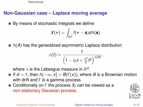
Non-Gaussian case – Laplace moving average

By means of stochastic integrals we define

X (τ ) =

∫Rd

f (τ − s)dΛ(s).

Λ(A) has the generalized asymmetric Laplace distribution

φ(t) =1(

1− iµt + σ2

2 t2)λ(A)

,

where λ is the Lebesgue measure in Rd .If d = 1, then Λ(−∞, x ] = B(Γ(x)), where B is a Brownian motionwith drift and Γ is a gamma process.Conditionally on Γ the process Xt can be viewed as anon-stationary Gaussian process.


Rice’s formula

Non-Gaussian case – why it is interesting

For a covariance R a matching symmetric kernel is given byfsym = F−1

√FR,

Symmetric kernels can not produce front-back asymmetries evenif the moving average process is not GaussianOrnstein-Uhlenbeck autocorrelation e−|x | can be obtained both bysymmetric and asymmetric kernels

0 200 400 600 800 1000

−2

0

2 0

0

0 200 400 600 800 1000

−2

0

2

4

0 0

0 200 400 600 800 1000

−2

0

2 0

0

0 200 400 600 800 1000

−2

0

2 0

0

0 200 400 600 800 1000

−5

0

5

0 0

0 200 400 600 800 1000

−2

0

2 0

0


Rice’s formula

Slope distributions at level crossings

derivative at down/upcrossing

leve

l

−6 −4 −2 0 2 4 6−6

−4

−2

0

2

4

6

0 0


leve

l

−6 −4 −2 0 2 4 6−5

−4

−3

−2

−1

0

1

2

3

4

5

0 0


leve

l

−6 −4 −2 0 2 4 6−3

−2

−1

0

1

2

3

4

5

6

0 0


leve

l

−6 −4 −2 0 2 4 6−3

−2

−1

0

1

2

3

4

5

6

0 0


Rice’s formula

Biased sampling in non-Gaussian case – why it is difficult

Biased sampling distribution

Pu(A) =E[{Y ∈ A}|X (0)|

∣∣X (0) = u]

E[|X (0)|

∣∣X (0) = u] ,

requires joint distribution of Y (·) and (X (0),X (0)).This can be difficult if (Y ,X ) are not jointly GaussianWhen X is non-Gaussian even the denominator can be a problem


Rice’s formula

Illustration of difficulties – crossing intensity

The joint distribution of X (0) and X (0)

φX ,X (ξ1, ξ2) = exp(−∫ ∞

0ln(

1 +12

(ξ21 + ξ2

2λ2)

)dF (λ)

).

the process and its derivative are uncorrelated but not independent asit is in a Gaussian case

by inverse Fourier transform

fX ,X (u, z) =1

(2π)2

∫ ∞−∞

∫ ∞−∞

e−i(ξ1u+ξ2z)φX ,X (ξ1, ξ2) dξ1 dξ2.

the crossing intensity can be computed by evaluating the integral

µ+(u) =1

4π2

∫ ∞0

∫ ∞−∞

∫ ∞−∞

ze−i(ξ1u+ξ2z)φX ,X (ξ1, ξ2) dξ1 dξ2 dz.


Slepian model

Representing biased sampling distributions

X – a stationary process having a.s. absolutely continuous sample and fX ,X ofX (0), X (0) exists.upcrossing set within interval [0, 1] is defined as

C(u) = {s ∈ [0, 1] : X (s) = u, X (s) > u}.

N(u) – the number of elements in C(u).A – a property of trajectories of another stationary stochastic process YN(A|u) – the number of s ∈ C(u) such that Y (s + ·) ∈ A.

Crossing level distributions of Y :

Pu(A) =E [N(A|u)]E [N(u)]

.

Slepian model for Pu– any stochastic process Yu with distribution givenby the upcrossing distribution

P(Yu ∈ A) = Pu(A).


Slepian model

Slepian model in the Gaussian case

Z – a stationary Gaussian process Zthe Slepian model process Zu around u-upcrossing of Z is givenby

Zu(t) = u r(t)− R r(t) + ∆(t),

r be the covariance function of Z ,R is a standard Rayleigh variablea non-stationary Gaussian process ∆ having covariance

r(t , s) = r(t − s)− r(t)r(s)− r ′(t)r ′(s).

R and ∆ are independent


Slepian model

Random scaling – a simple non-Gaussian case

for non-random scaling X(t) =√

k Z (t), t ∈ R, the Slepian model is

Xu(t) = u r(t)−√

kRr ′(t) +√

k∆(t)

random scaling K , (assume a gamma distribution), then X(t) =√

K Z (t),Slepian model for X :

Xu(t) = u r(t)−√

K R r(t) +√

K ∆(t)

this is not the case!!!X(t) conditionally on (K = k , X = z,X = u) is represented by u r(t)− z r(t) +

√k∆(t)

(k , z) has to be replaced by the Slepian model (Ku , Xu).Ku is ‘biased’ to account for the fact that the behavior observed at u up-crossings forspecific u makes certain scalings more likely than other – ‘sampling bias’.a correct Slepian model for Xu is given by

Xu(t) = u r(t)−√

KuR r(t) +√

Ku∆(t),

fKu (k) =βp/2

21−p/2upKp(√

2βu)· kp−1 exp

(−

2βk + u2/k2

),


Slepian model through Slepian noise

Moving average process

A moving average process is a convolution of a kernel function with ainfinitesimal “white noise” process having variance equal to the discretizationstep.Gaussian moving average (GMA):

X (t) =∫ ∞−∞

g(s − t) dB(s)

Slepian model dBu(x) for the noise dB(x) at the crossing levels u of X

Bu(t) = Fu,g(t) + Gg(t) + B(t),

where the non-random compenent is

Fu,g(t) = u∫ t

0g,

the kernel only dependent random component

Gg(t) =(

R −∫

g dB)·∫ t

0g −

∫g dB ·

∫ t

0g,

and purely random noise represented by Brownian motion B(t).



Simulated Slepian noise

−4 −2 0 2 4

−6

−4

−2

02

4

t

−4 −2 0 2 4−

4−

20

24

t

−4 −2 0 2 4

−4

−2

02

4

t

−4 −2 0 2 4

−6

−4

−2

02

46

8

t

Top: Brownian motion(left), Deterministic partFu : u = 0.5, 1, 3, 5(right),Bottom: Bu for: u = 0.5(left), u = 5 (right).



Non-Gaussian process at crossing of Gaussian one

Y1(t), t ∈ R– filtered original process X (t):

Y1(t) =

∫h(s − t) dX (s) =

∫h ∗ g(s − t) dB(s).

Laplace motion – subordination of the Brownian motion by the gammamotion K , (K (1) has the gamma distribution with shape τ and scale 1/τ )Laplace moving average

Y2(t) =

∫f (s − t) dB ◦ K (s).

Jointly Y (t) = (Y1(t),Y2(t)) and X (t) are not GaussianBiased sampling distributions can be evaluated numerically,although it can be a computational chalenge

How to get a Slepian model in this case with somemanageable structiure?



From Slepian noise to Slepian model

By using the Slepian noise Bu(t) one can provide with any Slepianmodel for processes functionally dependent on this noiseBivariate Slepian model

Y1u(t) =

∫h(s − t) dX (s) =

∫h ∗ g(s − t) dBu(s),

Y2u(t) =

∫f (s − t) dBu ◦ K (s).

The main benefit is that all computational difficulties are in evaluating Bu,and thus avoiding computation of the joint distribution of the processeswith complex structure.



Samples from joint Slepian model

−10 −5 0 5 10

−6

−4

−2

02

46

8

t

−10 −5 0 5 10

−6

−4

−2

02

46

8

t

−10 −5 0 5 10

−6

−4

−2

02

46

8

t

−10 −5 0 5 10

−6

−4

−2

02

46

8

t

−10 −5 0 5 10

−6

−4

−2

02

46

8

t

−10 −5 0 5 10

−6

−4

−2

02

46

8t

Left: Samples from GMA X = Y1 – (top) and LMA Y2 – (bottom).Six samples of BM and for Y2 a single sample of gamma processMiddle: Joint Slepian model (Y1u ,Y2u) at the crossings of X at u = 0.5.Right: Analogous samples at u = 5.


Slepian model at crossings of non-Gaussian process

Moving averages driven by non-Gaussian noise

More challenging problem of finding of a Slepian model at crossings ofnon-Gaussian process – a moving average driven by a non-Gaussiannoise dL(s) – Laplace motion, i.e.

X (t) =

∫f (s − t) dL(s) =

∫f (s − t) dB ◦ K (s),

where K (t) is a gamma process.

Gamma process as a subordinator is by convenience – other classes ofLevy processes are possible.

Laplace motion is a pure jump process and generally there is no explicitexpression for the joint distribution of the process and its derivative.

Strategy:find the Slepian model for the Laplace noise B ◦ K ,obtaining the Slepian models by replacing the noisein the original moving averages by the Slepian noise.



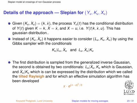
Details of the approach — Slepian for (Yu,Ku,Xu)

Given (Ku, Xu) = (k , x), the process Yu(t) has the conditional distributionof Y (t) given K = k , X = x , and X = u, i.e. Y (t |k , x ,u). This hasgaussian distribution..

Instead of (Ku, Xu) it happens easier to consider (Lu,Ku, Xu) by using theGibbs sampler with the conditionals

Ku|Lu, Xu and Lu, Xu|Ku

The first distribution is sampled from the generalized inverse Gaussian,the second is obtained by two conditionals: Lu|Xu,Ku which is Gaussian,and Xu|Ku which is can be expressed by the distribution which we calledthe tilted Rayleigh and for which an effective simulation algorithm hasbeen developed

x · e(x−a)2/b



Example

−10 −5 0 5 10

−6

−4

−2

02

46

t

−10 −5 0 5 10

−2

02

4

t

−10 −5 0 5 10

−8

−6

−4

−2

02

46

t

−10 −5 0 5 10

−4

−2

02

46

8

t

Left: Samples from BM (top)and LM (bottom)Right: Slepian model Lu atthe crossings of X at u = 0.5(top) and u = 5 (bottom).



Gaussian vs. Laplace Slepian model

−10 −5 0 5 10

−1.

0−

0.5

0.0

0.5

1.0

t

−10 −5 0 5 10

−4

−2

02

46

t

Left: Slepian noise BM (top)and LM (bottom), u = 5Right: Slepian model Xu atits own crossings at u = 0.5(top) and u = 5 (bottom).


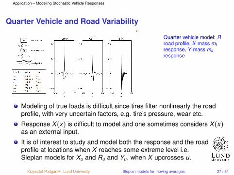
Application – Modeling Stochastic Vehicle Responses

Quarter Vehicle and Road Variability

Quarter vehicle model: Rroad profile, X mass mtresponse, Y mass msresponse

Modeling of true loads is difficult since tires filter nonlinearly the roadprofile, with very uncertain factors, e.g. tire’s pressure, wear etc.

Response X (x) is difficult to model and one sometimes considers X (x)as an external input.

It is of interest to study and model both the response and the roadprofile at locations when X reaches some extreme level i.e.Slepian models for Xu and Ru and Yu, when X upcrosses u.


Application – Modeling Stochastic Vehicle Responses

Two moving averages – the Gaussian and Laplace ones.

−100 −80 −60 −40 −20 0 20 40 60 80 100

−5

0

5

X(x)

−100 −80 −60 −40 −20 0 20 40 60 80 100

−5

0

5

R(x)

−100 −80 −60 −40 −20 0 20 40 60 80 100

−5

0

5

Y(x)

−40 −30 −20 −10 0 10 20 30 40

−10

−5

0

5

10

Xu(x)

−40 −30 −20 −10 0 10 20 30 40

−10

−5

0

5

10

Ru(x)

−40 −30 −20 −10 0 10 20 30 40

−10

−5

0

5

10

Yu(x)

−100 −80 −60 −40 −20 0 20 40 60 80 100

−5

0

5

X(x)

−100 −80 −60 −40 −20 0 20 40 60 80 100−5

0

5R(x)

−100 −80 −60 −40 −20 0 20 40 60 80 100

−5

0

5

Y(x)

−40 −30 −20 −10 0 10 20 30 40

−5

0

5

Xu(x)

−40 −30 −20 −10 0 10 20 30 40

−5

0

5

Ru(x)

−40 −30 −20 −10 0 10 20 30 40

−5

0

5

Yu(x)

The Laplace in the top threegraphs of each column andthe Gaussian case in thebottom three graphs of eachcolumn. Left: Road profileR(x) (middle) andresponses X(x) (top), Y (x)(bottom). Right: Slepianmodels Xu(x), Ru(x) andYu(x) around the u = 7upcrossing of X(x) in theLaplace case (top threegraphs) and around theu = 4.5 upcrossing of X(x)for the Gaussian case(bottom three graphs).


Conclusions

Conclusions

The level crossings distributions are important in studying extremal behavior ofstochastic processesGeneralized Rice’s formula is utilized to obtain effectively level crossingdistributionsThey are also important for studying asymmetries in the records, which requiresnon-Gaussian modelsSlepian model is a convenient way of representing level crossing distributionsSlepian model is quite straightforward in the Gaussian caseNon-Gaussian models requires special careAn approach through Slepian model for noise process is investigatedIt allows for simultaneous study different models arising from such a noise.A method of simulating from Slepian model in the case of Laplace noise isobtained exploring the dependence of the noise on the subordinating GammanoiseCrossing level behavior for non-Gaussian models is fundamentally different fromthe Gaussian counterpart


Conclusions

Thank you!


slepian models for moving averages driven by a non ...aila/slepian4laplace.pdf · rice’s formula...

Documents