slice sampling with multivariate steps - cs.toronto.eduradford/ftp/madeleine-thesis.pdfslice...
TRANSCRIPT
Slice Sampling with Multivariate Steps
by
Madeleine B. Thompson
A thesis submitted in conformity with the requirementsfor the degree of Doctor of Philosophy
Graduate Department of StatisticsUniversity of Toronto
Copyright c© 2011 by Madeleine B. Thompson

ii
Abstract
Slice Sampling with Multivariate Steps
Madeleine B. Thompson
Doctor of Philosophy
Graduate Department of Statistics
University of Toronto
2011
Markov chain Monte Carlo (MCMC) allows statisticians to sample from a wide variety
of multidimensional probability distributions. Unfortunately, MCMC is often difficult to
use when components of the target distribution are highly correlated or have disparate
variances. This thesis presents three results that attempt to address this problem. First,
it demonstrates a means for graphical comparison of MCMC methods, which allows re-
searchers to compare the behavior of a variety of samplers on a variety of distributions.
Second, it presents a collection of new slice-sampling MCMC methods. These methods
either adapt globally or use the adaptive crumb framework for sampling with multivariate
steps. They perform well with minimal tuning on distributions when popular methods
do not. Methods in the first group learn an approximation to the covariance of the tar-
get distribution and use its eigendecomposition to take non-axis-aligned steps. Methods
in the second group use the gradients at rejected proposed moves to approximate the
local shape of the target distribution so that subsequent proposals move more efficiently
through the state space. Finally, this thesis explores the scaling of slice sampling with
multivariate steps with respect to dimension, resulting in a formula for optimally choos-
ing scale tuning parameters. It shows that the scaling of untransformed methods can
sometimes be improved by alternating steps from those methods with radial steps based
on those of the polar slice sampler.
iii

Acknowledgements
I would like to thank my advisor, Radford Neal, for his support with this thesis and
the research leading up to it. Some material originally appeared in a technical report
coauthored with him, “Covariance Adaptive Slice Sampling” (Thompson and Neal, 2010).
iv
Contents
1 Introduction 1
1.1 Motivation . . . . . . . . . . . . . . . . . . . . . . . . . . . . . . . . . . . 1
1.2 Outline . . . . . . . . . . . . . . . . . . . . . . . . . . . . . . . . . . . . . 5
2 Measuring sampler efficiency 7
2.1 Autocorrelation time . . . . . . . . . . . . . . . . . . . . . . . . . . . . . 7
2.1.1 Batch mean estimator . . . . . . . . . . . . . . . . . . . . . . . . 8
2.1.2 Least squares fit to the log spectrum . . . . . . . . . . . . . . . . 9
2.1.3 Initial sequence estimators . . . . . . . . . . . . . . . . . . . . . . 9
2.1.4 AR process estimator . . . . . . . . . . . . . . . . . . . . . . . . . 10
2.1.5 Seven test series . . . . . . . . . . . . . . . . . . . . . . . . . . . . 11
2.1.6 Comparison of autocorrelation time estimators . . . . . . . . . . . 15
2.1.7 Multivariate distributions . . . . . . . . . . . . . . . . . . . . . . 17
2.2 Framework for comparing methods . . . . . . . . . . . . . . . . . . . . . 18
2.2.1 MCMC methods for comparison . . . . . . . . . . . . . . . . . . . 18
2.2.2 Distributions for comparison . . . . . . . . . . . . . . . . . . . . . 19
2.2.3 Processor time and log density evaluations . . . . . . . . . . . . . 21
2.3 Graphical comparison of methods . . . . . . . . . . . . . . . . . . . . . . 23
2.3.1 Between-cell comparisons . . . . . . . . . . . . . . . . . . . . . . . 25
2.3.2 Within-cell comparisons . . . . . . . . . . . . . . . . . . . . . . . 26
v

2.3.3 Comparison with multiple tuning parameters . . . . . . . . . . . . 27
2.3.4 Discussion of graphical comparison . . . . . . . . . . . . . . . . . 27
3 Samplers with multivariate steps 31
3.1 Slice sampling overview . . . . . . . . . . . . . . . . . . . . . . . . . . . . 31
3.2 Methods based on eigenvector decomposition . . . . . . . . . . . . . . . . 32
3.2.1 Univariate updates along eigenvectors . . . . . . . . . . . . . . . . 34
3.2.2 Evaluation of univariate updates . . . . . . . . . . . . . . . . . . 36
3.2.3 Multivariate updates with oblique hyperrectangles . . . . . . . . . 38
3.2.4 Evaluation of hyperrectangle updates . . . . . . . . . . . . . . . . 40
3.2.5 Convergence of the oblique hyperrectangle method . . . . . . . . 42
3.3 Irregular polyhedral slice approximations . . . . . . . . . . . . . . . . . . 44
3.4 Covariance matching . . . . . . . . . . . . . . . . . . . . . . . . . . . . . 47
3.4.1 Adaptive Gaussian crumbs . . . . . . . . . . . . . . . . . . . . . . 48
3.4.2 Adapting the crumb covariance . . . . . . . . . . . . . . . . . . . 49
3.4.3 Estimating the density at the mode . . . . . . . . . . . . . . . . . 54
3.4.4 Efficient computation of the crumb covariance . . . . . . . . . . . 54
3.5 Shrinking rank proposals . . . . . . . . . . . . . . . . . . . . . . . . . . . 56
3.6 Evaluation of the proposed methods . . . . . . . . . . . . . . . . . . . . . 62
3.6.1 Comparison on reference distributions . . . . . . . . . . . . . . . 62
3.6.2 Comparison on a latent AR process . . . . . . . . . . . . . . . . . 64
4 Scaling and radial steps 69
4.1 Optimal tuning of Gaussian crumbs . . . . . . . . . . . . . . . . . . . . . 69
4.1.1 Scaling on slices of known radius . . . . . . . . . . . . . . . . . . 69
4.1.2 Scaling on slices of χp radius . . . . . . . . . . . . . . . . . . . . . 73
4.2 Comparisons of non-adaptive Gaussian crumb methods . . . . . . . . . . 75
4.2.1 Comparison to ideal slice sampling . . . . . . . . . . . . . . . . . 75
vi
4.2.2 Polar slice sampling . . . . . . . . . . . . . . . . . . . . . . . . . . 78
4.2.3 Univariate steps . . . . . . . . . . . . . . . . . . . . . . . . . . . . 81
4.2.4 Discussion . . . . . . . . . . . . . . . . . . . . . . . . . . . . . . . 83
4.3 Practical algorithms for radial steps . . . . . . . . . . . . . . . . . . . . . 84
4.3.1 Radial steps using a gridded state space . . . . . . . . . . . . . . 84
4.3.2 Radial steps using auxiliary variables . . . . . . . . . . . . . . . . 85
4.3.3 Evaluation on a sequence of Gaussians . . . . . . . . . . . . . . . 88
4.3.4 Evaluation on two regressions . . . . . . . . . . . . . . . . . . . . 92
5 Conclusion 93
5.1 Contributions . . . . . . . . . . . . . . . . . . . . . . . . . . . . . . . . . 93
5.2 Limitations and future work . . . . . . . . . . . . . . . . . . . . . . . . . 95
5.3 Software . . . . . . . . . . . . . . . . . . . . . . . . . . . . . . . . . . . . 96
References 96
vii

viii
List of figures
2.1 Seven series comprising a test set . . . . . . . . . . . . . . . . . . . . . . 12
2.2 Autocorrelation times computed by four methods . . . . . . . . . . . . . 14
2.3 Autocorrelation function of the AR(2) series . . . . . . . . . . . . . . . . 15
2.4 AR process-generated confidence intervals . . . . . . . . . . . . . . . . . 16
2.5 Marginals and conditionals of GP (unlogged) . . . . . . . . . . . . . . . . 20
2.6 Ratio of processor usage to log density evaluations . . . . . . . . . . . . . 22
2.7 Demonstration of graphical comparison . . . . . . . . . . . . . . . . . . . 24
2.8 Demonstration with two tuning parameters . . . . . . . . . . . . . . . . . 28
2.9 Reduced-dimension representation of comparison . . . . . . . . . . . . . . 29
3.1 Comparison of Univar Eigen to two MCMC methods . . . . . . . . . . . 37
3.2 Comparison of Oblique Hyperrect to several MCMC methods . . . . . . 41
3.3 Three ways to update a hyperrectangular slice approximation . . . . . . 45
3.4 Visualization of covariance matching . . . . . . . . . . . . . . . . . . . . 50
3.5 Pseudocode for covariance matching . . . . . . . . . . . . . . . . . . . . . 57
3.6 Visualization of shrinking rank . . . . . . . . . . . . . . . . . . . . . . . . 58
3.7 Pseudocode for shrinking rank . . . . . . . . . . . . . . . . . . . . . . . . 61
3.8 Comparison of MCMC methods . . . . . . . . . . . . . . . . . . . . . . . 63
3.9 Realization of a latent AR process . . . . . . . . . . . . . . . . . . . . . . 65
3.10 Comparison of MCMC methods on latent AR processes . . . . . . . . . . 67
3.11 Reduced-dimension representation of comparison . . . . . . . . . . . . . . 68
ix
4.1 Distance squared traveled on unit p-balls . . . . . . . . . . . . . . . . . . 70
4.2 Distance squared traveled on p-balls of χp radius . . . . . . . . . . . . . . 74
4.3 Autocorrelation time of simulations on Gaussians . . . . . . . . . . . . . 76
4.4 Evaluations per iteration of simulations on Gaussians . . . . . . . . . . . 77
4.5 Pseudocode for a combined standard-radial step . . . . . . . . . . . . . . 79
4.6 Performance of Gaussian crumbs and ideal slice sampling . . . . . . . . . 80
4.7 Cost of uncorrelated draws from Gaussians . . . . . . . . . . . . . . . . . 82
4.8 Pseudocode for a gridded radial step . . . . . . . . . . . . . . . . . . . . 86
4.9 Scaling of radial steps with respect to target dimension . . . . . . . . . . 89
4.10 Cost of radial steps on two regressions . . . . . . . . . . . . . . . . . . . 91
x
Chapter 1
Introduction
1.1 Motivation
When researchers need to perform a statistical analysis, they usually reach for standard
tools like t-tests, linear regression, and ANOVA. The results may not be easy to interpret
correctly, but they are at least easy to generate. The methods have a gentle learning
curve, allowing users with minimal sophistication to interpret the most straightforward
aspects of their results. One can, for instance, make use of a regression line without
understanding diagnostics like Cp (Mallows, 1973). As a user becomes more familiar
with a method, they can draw richer conclusions and perform more subtle analyses.
They do not need to understand the inner workings of the method the first time they use
it. LOESS illustrates this phenomenon. While it has many free parameters, a LOESS
fit can be computed entirely automatically. Users do not even know what they are
estimating—they just ask their statistics software to fit a curve to their data.
It is my hope that this simplicity can be extended to a wider variety of models.
Currently, balanced ANOVA is used more often than more general multilevel models of
the sort described by Gelman et al. (2004, ch. 5) because the more general models must
be specified in a language at least as complex as that of BUGS (Spiegelhalter et al.,
1
2 Chapter 1. Introduction
1995, §4). Users must learn to tune a Markov chain Monte Carlo (MCMC) sampler
(Neal, 1993) and analyze the results for convergence. They must also learn how to
display the simulation results in a way that can be understood. The MCMC sampler
tuning step is the most difficult aspect of this procedure; each of the other steps must
also be performed in ANOVA, which runs entirely automatically. The necessity of user
involvement in fitting the model forces the user to manage the entire process themself.
The hope that a wider variety of models could be fit with the ease of LOESS or ANOVA
motivates the research described in this document.
In particular, this thesis focuses on the development of MCMC methods that are
applicable to a wide variety of probability distributions without manual tuning. Most of
those who use MCMC use some variation on Gibbs sampling (Neal, 1993, §4.1). Gibbs
sampling is only possible when one knows the full conditional distributions of the compo-
nents of the distribution, largely restricting its use to models with Gaussian, gamma, and
binomial conditional distributions. Even on those models, it only performs well when
those components are not highly correlated.
The class of models that can be modeled with Gibbs sampling can be expanded
to allow for components with log-concave distributions of unknown form by applying
adaptive rejection sampling (abbreviated ARS, Gilks and Wild, 1992). ARS requires users
to specify an initial envelope for the conditional, though this can often be automatically
determined. Further expansion to include those models with non-log-concave conditionals
is possible with the use of adaptive rejection Metropolis sampling (abbreviated ARMS,
Gilks et al., 1995). Like ARS, ARMS requires the user to specify an initial envelope, but
with ARMS, a simulation could miss modes if the envelope is badly chosen. A proper
envelope may depend on the values of the conditioning variables, so ARMS is also often
difficult to properly configure. More commonly, users use random-walk Metropolis to
update a single coordinate at a time, though it is often much less efficient than Gibbs
sampling or ARMS and requires careful tuning.
1.1. Motivation 3
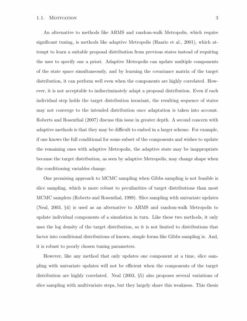
An alternative to methods like ARMS and random-walk Metropolis, which require
significant tuning, is methods like adaptive Metropolis (Haario et al., 2001), which at-
tempt to learn a suitable proposal distribution from previous states instead of requiring
the user to specify one a priori. Adaptive Metropolis can update multiple components
of the state space simultaneously, and by learning the covariance matrix of the target
distribution, it can perform well even when the components are highly correlated. How-
ever, it is not acceptable to indiscriminately adapt a proposal distribution. Even if each
individual step holds the target distribution invariant, the resulting sequence of states
may not converge to the intended distribution once adaptation is taken into account.
Roberts and Rosenthal (2007) discuss this issue in greater depth. A second concern with
adaptive methods is that they may be difficult to embed in a larger scheme. For example,
if one knows the full conditional for some subset of the components and wishes to update
the remaining ones with adaptive Metropolis, the adaptive state may be inappropriate
because the target distribution, as seen by adaptive Metropolis, may change shape when
the conditioning variables change.
One promising approach to MCMC sampling when Gibbs sampling is not feasible is
slice sampling, which is more robust to peculiarities of target distributions than most
MCMC samplers (Roberts and Rosenthal, 1999). Slice sampling with univariate updates
(Neal, 2003, §4) is used as an alternative to ARMS and random-walk Metropolis to
update individual components of a simulation in turn. Like these two methods, it only
uses the log density of the target distribution, so it is not limited to distributions that
factor into conditional distributions of known, simple forms like Gibbs sampling is. And,
it is robust to poorly chosen tuning parameters.
However, like any method that only updates one component at a time, slice sam-
pling with univariate updates will not be efficient when the components of the target
distribution are highly correlated. Neal (2003, §5) also proposes several variations of
slice sampling with multivariate steps, but they largely share this weakness. This thesis
4 Chapter 1. Introduction
extends his work on multivariate steps and proposes several slice sampling methods that
take multivariate steps that respect the local shape of the target distribution. Using
either previously visited states or the gradient of the log density at rejected moves, these
slice samplers can be efficient even when the distribution is badly scaled and the param-
eters are highly correlated, which is often the case with the multivariate models I hope
to make more broadly accessible.
In high-dimensional spaces, some methods that update multiple components at once
can move efficiently along the contours of a target distribution but not between them.
Roberts and Rosenthal (2002) propose the “polar slice sampler,” a variation of slice
sampling that operates in polar coordinates relative to a single, known mode. In this
coordinate system, the sampler mixes efficiently with respect to the log density. However,
the polar slice sampler uses non-adaptive rejection sampling to draw proposed moves,
which is often prohibitively inefficient, so it has not been used much. This thesis extends
the work of Roberts and Rosenthal, developing a practical means to modify an MCMC
method so that it can move efficiently between contours of a target distribution. The
proposed methods take radial steps similar to those of the polar slice sampler, but use a
secondary MCMC method to move in the angular coordinates so that rejection sampling
is not needed.
Development of new MCMC methods motivated another question: how can we iden-
tify the circumstances under which one MCMC method is superior to other methods? To
address this, I propose several figures of merit for MCMC samplers and develop schemes
for presenting the merits of a range of samplers and test distributions so that I and other
researchers can place newly developed methods in a broader context.
1.2. Outline 5
1.2 Outline
Chapter 2 compares figures of merit for MCMC samplers and the means to present
them. First, I discuss how the mixing efficiency of a Markov chain can be described by
its autocorrelation time and describe several methods for estimating this. I describe a
test set developed for these methods, which I use to justify a preference for a method
that models a Markov chain as an autoregressive process. Autocorrelation time only
considers the state sequence of a Markov chain, not the resources used to compute it,
so it is not an acceptable figure of merit on its own. I describe how one can build on
autocorrelation time to compute a more appropriate figure of merit, log density function
evaluations per uncorrelated observation. Then, I demonstrate how this measure can
be used to make graphical comparisons of collections of MCMC methods with a range
of tuning parameters on several distributions simultaneously. These comparisons allow
researchers to see how particular MCMC methods fit into a broader context.
Chapter 3 contains the principal results of this research, several variations on slice
sampling that take multivariate steps. The first two methods are inspired by adaptive
Metropolis. They adaptively choose slice approximations using the eigendecomposition of
the sample covariance matrix of the target distribution. These methods often work well,
but have limitations that come from retaining state from iteration to iteration. To address
these, I first describe a simple but unworkable method that uses gradients at rejected
points to create a temporary polyhedral approximation to the slice. It is computationally
infeasible, but motivates the use of the crumb framework, which allows for methods with
more computationally tractable proposal distributions. I then describe one such method
in the crumb framework, covariance matching. Using log density gradients at rejected
proposals, covariance matching chooses crumb distributions so that the covariances of
the proposal distributions approximate the covariance of uniform sampling over the slice.
This is followed by a description of a second method in the crumb framework, shrinking
rank, which also uses gradients to adapt to local structure of the target distribution. It

6 Chapter 1. Introduction
is more computationally efficient and simpler than covariance matching, and retains its
most desirable properties. The chapter closes with a comparison of the proposed MCMC
methods using the evaluation methods of chapter 2.
While chapter 3 focuses on efficient sampling with respect to linear functions of the
components of the state space of the target distribution, chapter 4 focuses on efficient
sampling with respect to the log density of the target distribution and addresses the
closely related topic of scaling with increasing dimension. It describes experiments that
explore the scaling behavior and proper tuning of samplers in the crumb framework. It
shows that samplers in the crumb framework commonly have linear scaling with respect
to the dimension of the target distribution and that this can be improved under some cir-
cumstances. It extends these results to more practical samplers, showing how combining
univariate radial steps with a method like covariance matching can result in improved
scaling with respect to log density.
Finally, chapter 5 describes the circumstances under which both the MCMC methods
and the techniques used to analyze them may be more broadly applied. It also provides
references to software that implements the methods described in this document.
Chapter 2
Measuring sampler efficiency
To compare the performance of MCMC methods using a collection of simulations, we
must be able to quantify the efficiency of a single simulation, and we must have a means
to display a collection of these measurements. In this chapter, I break down the efficiency
of a simulation into measurements of the correlation between observations and the cost
of obtaining an observation. Then, I demonstrate several types of plots for comparing
the efficiency of collections of simulations representing different samplers, distributions,
and tuning parameters.
2.1 Autocorrelation time
Autocorrelation time measures the convergence rate of the sample mean of a function of
a stationary, geometrically ergodic Markov chain with finite variance. Let {Xi}ni=1 be n
values of a scalar function of the states of such a Markov chain, where EXi = µ and
varXi = σ2. Let Xn be the sample mean of (X1, . . . , Xn). Then, the autocorrelation
time is the value of τ such that:√n
τ· Xn − µ
σ=⇒ N(0, 1) (2.1)
7
8 Chapter 2. Measuring sampler efficiency
Conceptually, the autocorrelation time is the number of Markov chain transitions equiv-
alent to a single uncorrelated draw from the distribution of {Xi}. It can be a useful
summary of the efficiency of an MCMC sampler. However, one must be cautious when
using it with adaptive methods such as those discussed in section 3.2 because they do
not have stationary distributions, and equation 2.1 does not strictly apply.
Since there is rarely a closed-form expression for the autocorrelation time, many
methods for estimating it from sampled data have been developed. The following sections
describe four such methods in wide use: computing batch means, fitting a linear regression
to the log spectrum, summing an initial sequence of the sample autocorrelation function,
and modeling as an autoregressive process. Then, these methods are compared on a test
set of seven series. For a broader context, two classic overviews of uncertainty in MCMC
estimation are Geyer (1992) and Neal (1993, §6.3). An alternative to autocorrelation
time, potential scale reduction, is discussed by Gelman and Rubin (1992).
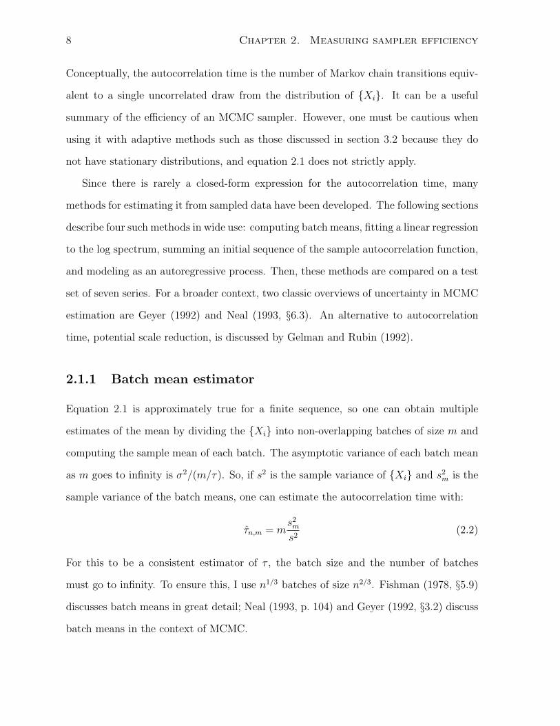
2.1.1 Batch mean estimator
Equation 2.1 is approximately true for a finite sequence, so one can obtain multiple
estimates of the mean by dividing the {Xi} into non-overlapping batches of size m and
computing the sample mean of each batch. The asymptotic variance of each batch mean
as m goes to infinity is σ2/(m/τ). So, if s2 is the sample variance of {Xi} and s2m is the
sample variance of the batch means, one can estimate the autocorrelation time with:
τn,m = ms2m
s2(2.2)
For this to be a consistent estimator of τ , the batch size and the number of batches
must go to infinity. To ensure this, I use n1/3 batches of size n2/3. Fishman (1978, §5.9)
discusses batch means in great detail; Neal (1993, p. 104) and Geyer (1992, §3.2) discuss
batch means in the context of MCMC.
2.1. Autocorrelation time 9
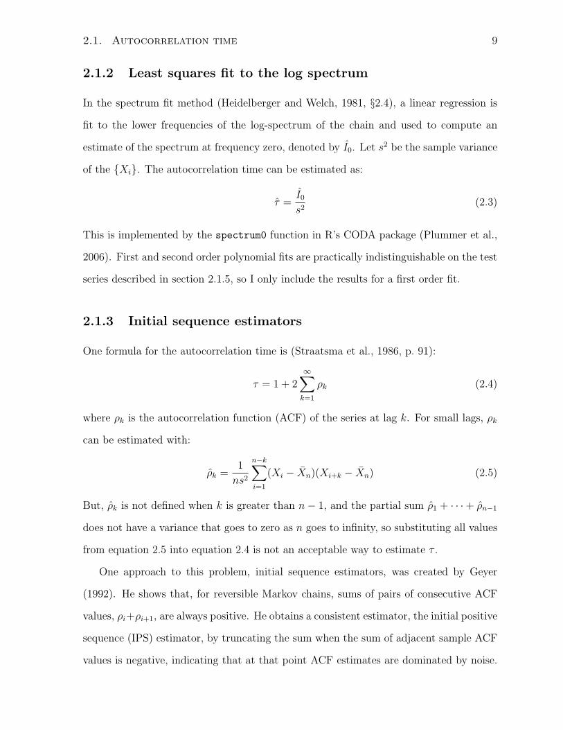
2.1.2 Least squares fit to the log spectrum
In the spectrum fit method (Heidelberger and Welch, 1981, §2.4), a linear regression is
fit to the lower frequencies of the log-spectrum of the chain and used to compute an
estimate of the spectrum at frequency zero, denoted by I0. Let s2 be the sample variance
of the {Xi}. The autocorrelation time can be estimated as:
τ =I0
s2(2.3)
This is implemented by the spectrum0 function in R’s CODA package (Plummer et al.,
2006). First and second order polynomial fits are practically indistinguishable on the test
series described in section 2.1.5, so I only include the results for a first order fit.
2.1.3 Initial sequence estimators
One formula for the autocorrelation time is (Straatsma et al., 1986, p. 91):
τ = 1 + 2∞∑k=1
ρk (2.4)
where ρk is the autocorrelation function (ACF) of the series at lag k. For small lags, ρk
can be estimated with:
ρk =1
ns2
n−k∑i=1
(Xi − Xn)(Xi+k − Xn) (2.5)
But, ρk is not defined when k is greater than n− 1, and the partial sum ρ1 + · · ·+ ρn−1
does not have a variance that goes to zero as n goes to infinity, so substituting all values
from equation 2.5 into equation 2.4 is not an acceptable way to estimate τ .
One approach to this problem, initial sequence estimators, was created by Geyer
(1992). He shows that, for reversible Markov chains, sums of pairs of consecutive ACF
values, ρi+ρi+1, are always positive. He obtains a consistent estimator, the initial positive
sequence (IPS) estimator, by truncating the sum when the sum of adjacent sample ACF
values is negative, indicating that at that point ACF estimates are dominated by noise.
10 Chapter 2. Measuring sampler efficiency
Further, the sequence of sums of pairs is always decreasing, so one can smooth the initial
positive sequence when a sum of two adjacent sample ACF values is larger than the
sum of the previous pair; the resulting estimator is the initial monotone sequence (IMS)
estimator. Finally, the sequence of sums of pairs is also convex. Smoothing the sum to
account for this results in the initial convex sequence (ICS) estimator. For more details,
see Geyer (1992, §3.3). I was unable to distinguish the behavior of the IPS, IMS, and ICS
estimators on the series of section 2.1.5, so the comparisons of section 2.1.6 only include
the ICS estimator.
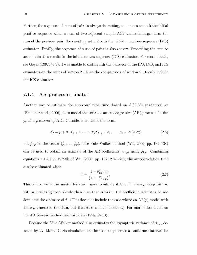
2.1.4 AR process estimator
Another way to estimate the autocorrelation time, based on CODA’s spectrum0.ar
(Plummer et al., 2006), is to model the series as an autoregressive (AR) process of order
p, with p chosen by AIC. Consider a model of the form:
Xt = µ+ π1Xt−1 + · · ·+ πpXt−p + at, at ∼ N(0, σ2a) (2.6)
Let ρ1:p be the vector (ρ1, . . . , ρp). The Yule–Walker method (Wei, 2006, pp. 136–138)
can be used to obtain an estimate of the AR coefficients, π1:p, using ρ1:p. Combining
equations 7.1.5 and 12.2.8b of Wei (2006, pp. 137, 274–275), the autocorrelation time
can be estimated with:
τ =1− ρT1:pπ1:p(1− 1Tp π1:p
)2 (2.7)
This is a consistent estimator for τ as n goes to infinity if AIC increases p along with n,
with p increasing more slowly than n so that errors in the coefficient estimates do not
dominate the estimate of τ . (This does not include the case where an AR(p) model with
finite p generated the data, but that case is not important.) For more information on
the AR process method, see Fishman (1978, §5.10).
Because the Yule–Walker method also estimates the asymptotic variance of π1:p, de-
noted by Vπ, Monte Carlo simulation can be used to generate a confidence interval for
2.1. Autocorrelation time 11
the autocorrelation time. Draw (π(1), π(2), . . .) from the distribution:
π(i) ∼ N(π1:p, Vπ) (2.8)
When the roots of 1 = π(i)1 z + · · · + π
(i)p zp all lie outside the unit circle, π(i) produces
a stationary time series (Wei, 2006, p. 47, equation 3.1.28). The corresponding auto-
correlation function, ρ(i), can be computed with the R function ARMAacf. Substituting
π(i) and ρ(i) into equation 2.7 gives a simulated draw from the distribution of τ . When
at least one root lies inside or on the unit circle, π(i) produces a nonstationary process
(Wei, 2006, p. 26), and τ is not defined; an estimate of infinity is used in this case. After
simulating a sample of a reasonable size, the quantiles of the sample can be used as a
confidence interval for τ . If more than 2.5% of the simulated π(i) define nonstationary
processes, the resulting 95% confidence interval is unbounded.
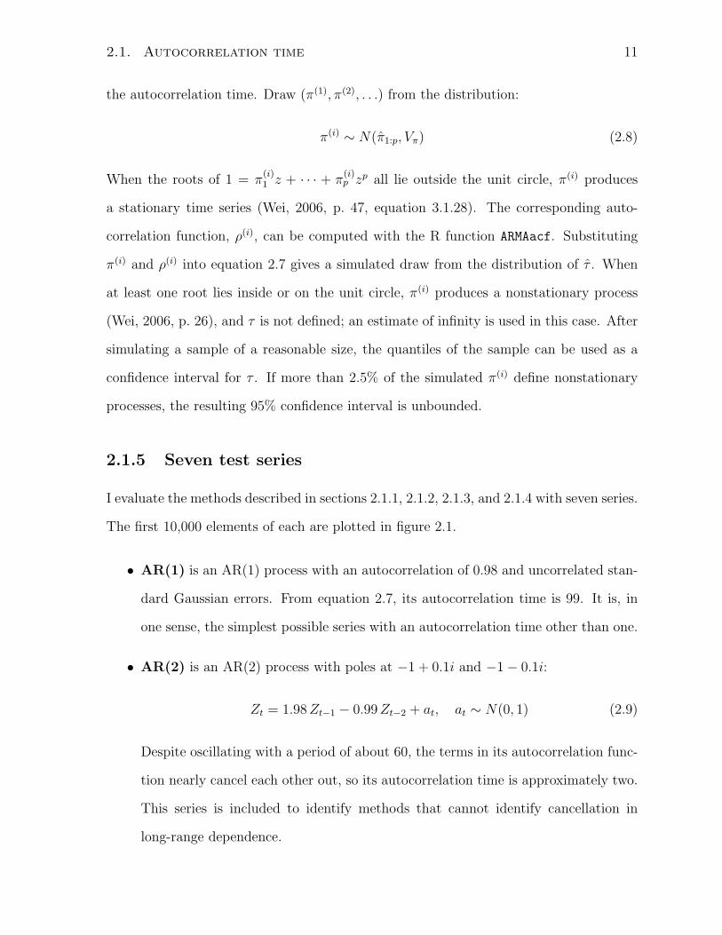
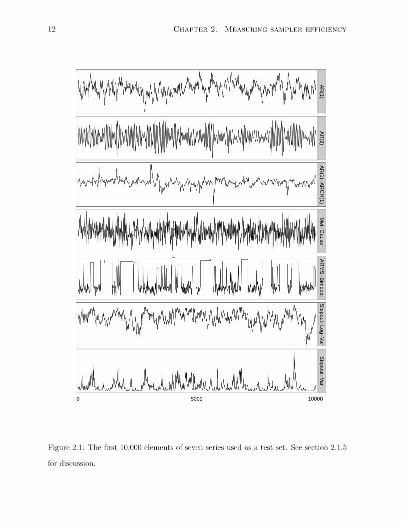
2.1.5 Seven test series
I evaluate the methods described in sections 2.1.1, 2.1.2, 2.1.3, and 2.1.4 with seven series.
The first 10,000 elements of each are plotted in figure 2.1.
• AR(1) is an AR(1) process with an autocorrelation of 0.98 and uncorrelated stan-
dard Gaussian errors. From equation 2.7, its autocorrelation time is 99. It is, in
one sense, the simplest possible series with an autocorrelation time other than one.
• AR(2) is an AR(2) process with poles at −1 + 0.1i and −1− 0.1i:
Zt = 1.98Zt−1 − 0.99Zt−2 + at, at ∼ N(0, 1) (2.9)
Despite oscillating with a period of about 60, the terms in its autocorrelation func-
tion nearly cancel each other out, so its autocorrelation time is approximately two.
This series is included to identify methods that cannot identify cancellation in
long-range dependence.
12 Chapter 2. Measuring sampler efficiency
0 5000 10000
AR
(1)A
R(2)
AR
(1)−A
RC
H(1)
Met−
Gauss
AR
MS
−B
imodal
Stepout−
Log−V
arS
tepout−V
ar
Figure 2.1: The first 10,000 elements of seven series used as a test set. See section 2.1.5
for discussion.
2.1. Autocorrelation time 13
• AR(1)-ARCH(1) is an AR(1) process with autocorrelation of 0.98 and autocor-
related errors:
Zt = 0.98Zt−1 + at, at ∼ N(0, 0.01 + 0.99 a2
t−1
)(2.10)
Its autocorrelation time is also 99. This series could confound methods that assume
constant step variance.
• Met-Gauss is a sequence of states generated by a Metropolis sampler with stan-
dard Gaussian proposals sampling from a standard Gaussian target distribution.
It has a proposal acceptance rate of 0.7 and an autocorrelation time of eight. It is
a simple example of a state sequence from an MCMC sampler.
• ARMS-Bimodal is also a sequence of states from an MCMC simulation, ARMS
(Gilks et al., 1995) applied to a mixture of two Gaussians. The sampler is badly
tuned, so it rarely accepts a proposal when near the upper mode. It has an auto-
correlation time of approximately 200.
• Stepout-Log-Var is a third MCMC sequence, the log-variance parameter of slice
sampling with stepping out (Neal, 2003, §4) sampling from a ten-parameter multi-
level model (Gelman et al., 2004, pp. 138–145). Its autocorrelation time is approx-
imately 200.
• Stepout-Var was generated by exponentiating the states of Stepout-Log-Var. Be-
cause its sample mean is dominated by large observations, its autocorrelation time,
approximately 100, is different than that of Stepout-Log-Var. Like ARMS-Bimodal
and Stepout-Log-Var, it is a challenging, real-world example of a sequence whose
autocorrelation time might be unknown.
14 Chapter 2. Measuring sampler efficiency
series length
auto
corr
elat
ion
time
0.1
1
10
100
0.1
1
10
100
AR(1)
i
ii
ii i
i ii i i i i i i
a
a
a aa a
a aa a a a a a a
s
ss
ss
s
s
ss s s s s s
b
b
bb b
bb
b
bb b b b
b b
ARMS−Bimodal
i i i i
ii
i
i i i i i i i i
aa
a
a
a
a
a
a a aa a a a a
s
ss s
ss
s
ss
ss s s s s
b
b
b
b
b
b
b
b b bb b b b b
10 1001,000
10,000100,000
AR(2)
i
i
i i i i i i i i i i i i i
a
a
a
a
aa a
a a a a a a a a
s s s s
s
s
s
s
ss s
s s
b b
bb
b bb
b bb b b
b b b
Stepout−Log−Var
i ii
i ii
i i i i i i i i i
a aa
a a a
a a a a a a a a a
s s ss
ss
s
s
ss
s s s s s
b
b
b
bb b
bb b b
b b b b b
10 1001,000
10,000100,000
AR(1)−ARCH(1)
i
i
i ii i i
i
i i i i i i i
a
a
aa
a a a aa a a a a a a
ss
s s
ss
s
ss
s s s ss s
b b
bb
b b bb
b bb b b b b
Stepout−Var
i i i
ii i
i i i i i i i i i
a a a
a a a
a a a a a a a a a
s s s s
ss
s
ss
s s s s s s
b
b
b
b b b
bb b b b b b b b
10 1001,000
10,000100,000
Met−Gauss
i ii i i i i i i i i i i i i
a aa
a aa a a a a a a a a a
s s s ss s s s
s s s ss s s
bb
b b
bb
bb
b b b bb b b
10 1001,000
10,000100,000
method
i ICS
a AR process
s Spec. fit
b Batch means
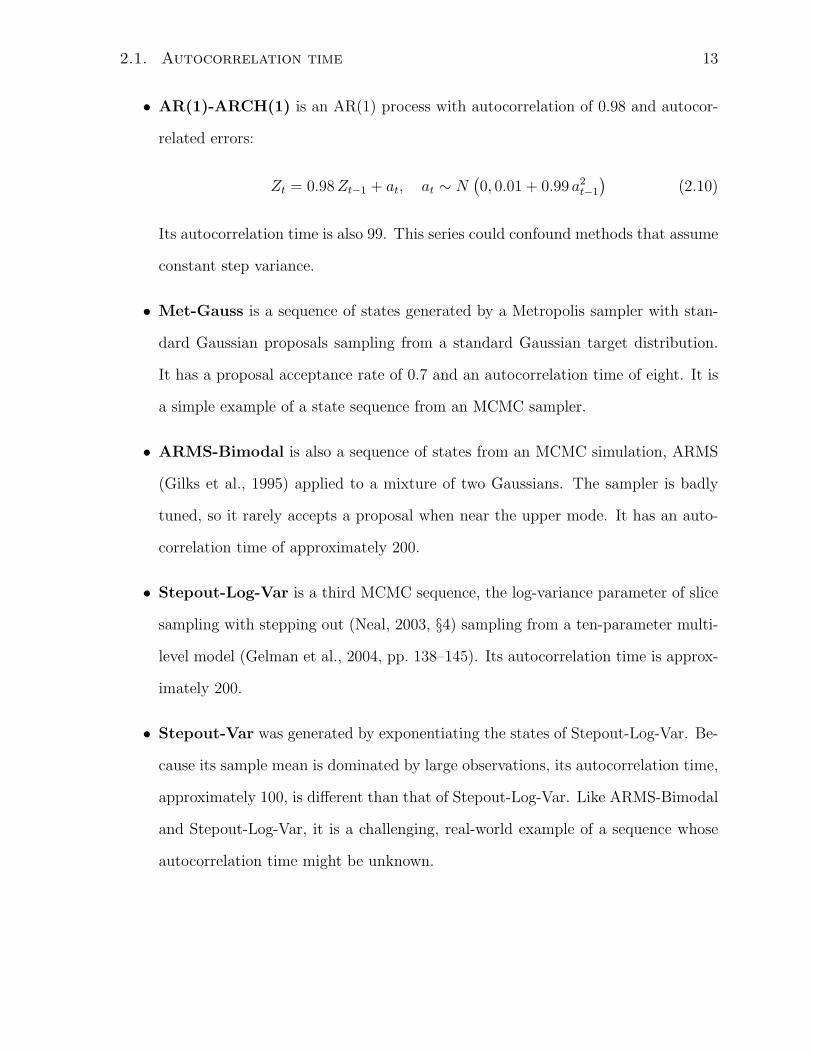
Figure 2.2: Autocorrelation times computed by four methods on seven series for a range
of subsequence lengths. Each plot symbol represents a single estimate. The dashed
line indicates the true autocorrelation time. Breaks in the lines for spectrum fit indicate
instances where the method failed to produce an estimate. See section 2.1.6 for discussion.
2.1. Autocorrelation time 15
lag
−0.5
0.0
0.5
1.0
0 20 40 60 80 100 120 140
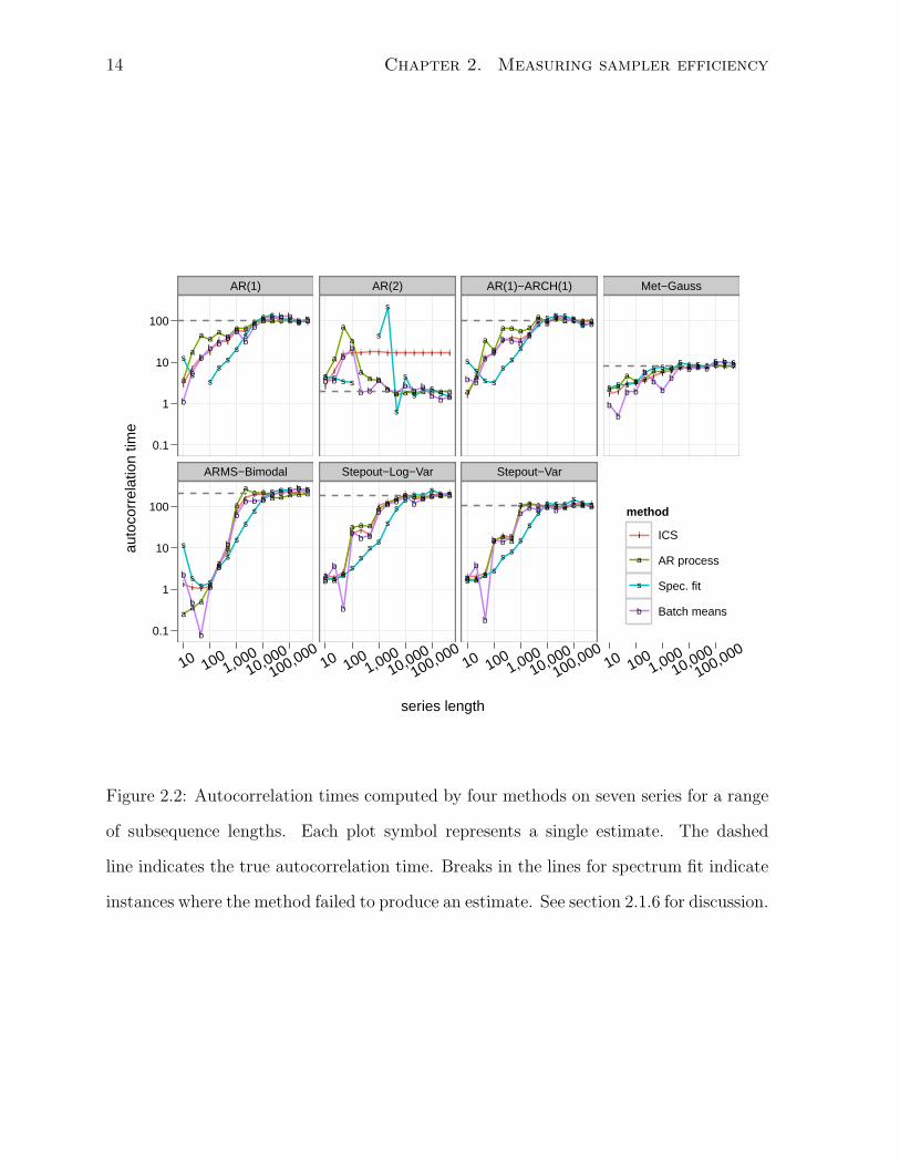
Figure 2.3: The autocorrelation function of the AR(2) series. See section 2.1.6 for dis-
cussion.
2.1.6 Comparison of autocorrelation time estimators
This section compares the true autocorrelation time of each series to the autocorrelation
time estimated by each method for subsequences ranging in length from 10 to 500,000.
The results are plotted in figure 2.2. All four methods converge to the true value on all
seven chains, with the exception of ICS on the AR(2) process. In general, the AR process
method converges to the true autocorrelation time fastest, followed by ICS, batch means,
and finally spectrum fit, which does not even produce an estimate in all cases. All four
methods tend to underestimate autocorrelation times for all short sequences except those
from the AR(2) process, which appears in small samples to have a longer autocorrelation
time than it actually does.
ICS is inconsistent on the AR(2) process because the autocorrelation function of the
AR(2) process is significant at lags larger than its first zero-crossing (see figure 2.3).
ICS and the other initial sequence estimators are not necessarily consistent when the
underlying chain is not reversible; the AR(2) process is not, when considered as a two
state system with the Markov property. These estimators stop summing the sample
16 Chapter 2. Measuring sampler efficiency
series length
auto
corr
elat
ion
time
0.01
0.1
1
10
100
1,000
0.01
0.1
1
10
100
1,000
AR(1)
a
aa a a a
a a a a a a a a a
ARMS−Bimodal
a a aa
aa
aa a a a a a a a
10 1001,000
10,000100,000
AR(2)
aa
aa
a a aa a a a a a a a
Stepout−Log−Var
a a a
a a aa a a a a a a a a
10 1001,000
10,000100,000
AR(1)−ARCH(1)
aa
aa
a a a aa a a a a a a
Stepout−Var
a a a
a a a
a a a a a a a a a
10 1001,000
10,000100,000
Met−Gauss
a aa a a
a a a a a a a a a a
10 1001,000
10,000100,000
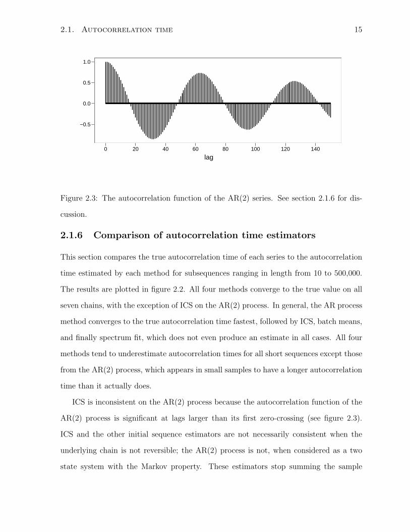
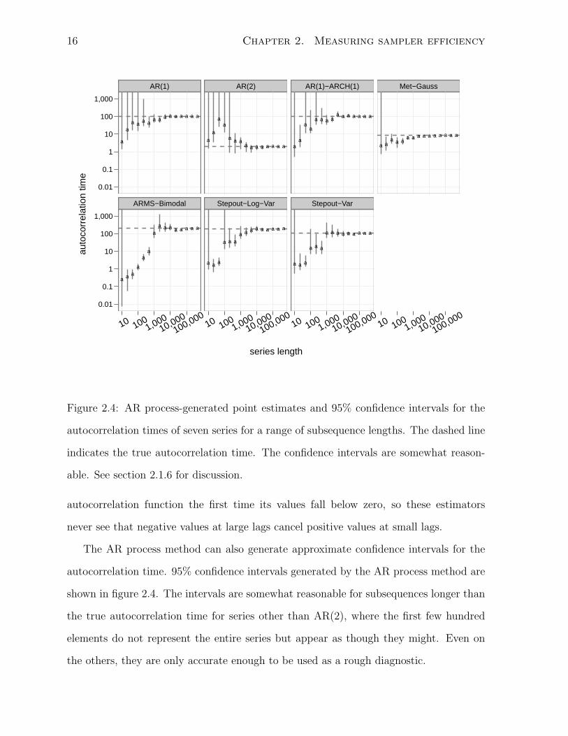
Figure 2.4: AR process-generated point estimates and 95% confidence intervals for the
autocorrelation times of seven series for a range of subsequence lengths. The dashed line
indicates the true autocorrelation time. The confidence intervals are somewhat reason-
able. See section 2.1.6 for discussion.
autocorrelation function the first time its values fall below zero, so these estimators
never see that negative values at large lags cancel positive values at small lags.
The AR process method can also generate approximate confidence intervals for the
autocorrelation time. 95% confidence intervals generated by the AR process method are
shown in figure 2.4. The intervals are somewhat reasonable for subsequences longer than
the true autocorrelation time for series other than AR(2), where the first few hundred
elements do not represent the entire series but appear as though they might. Even on
the others, they are only accurate enough to be used as a rough diagnostic.
2.1. Autocorrelation time 17
The AR process method is marginally more accurate than the three other methods
and is the only method that, as implemented, generates confidence intervals, so I usually
prefer it to the other three. The batch mean estimate is faster to compute and almost
as accurate, so it is useful when speed is important and confidence intervals are not
necessary.
2.1.7 Multivariate distributions
So far, I have considered the estimation of autocorrelation time for a scalar function of
the state of a Markov chain. Often, however, users are interested in how fast the Markov
chain as a whole mixes. Let Y be a linear combination of two scalar functions of state,
X(1) and X(2):
Y = aX(1) + bX(2) (2.11)
If the two functions have autocorrelation times τ (1) and τ (2), the variance of the sample
mean of Y will be:
var(Yn) = a2 var(X(1)n ) + 2ab cov(X(1)
n , X(2)n ) + b2 var(X(2)
n ) (2.12)
= a2 var(X(1)) + 2ab√
var(X(1)) var(X(2)) corr(X(1)n , X(2)
n ) + b2 var(X(2))
≈ a2 τ(1)
nvar(X(1)) + 2ab
√τ (1)τ (2)
n
√var(X(1)) var(X(2)) corr(X(1)
n , X(2)n ) (2.13)
+ b2 τ(2)
nvar(X(2))
=1
n
(τ (1)A+ 2
√τ (1)A
√τ (2)B corr(X(1)
n , X(2)n ) + τ (2)B
)(2.14)
≤ 4
nmax
(τ (1)A, τ (2)B
)(2.15)
where A = a2 varX(1) and B = b2 varX(2). If the terms of the combination are not
anti-correlated (so that there is no possibility the sample means cancel each other out)
and the sample means come from independent observations, the variance of the sample
mean of Y is asymptotically bounded below by 1n(A + B). The bound of equation 2.15
is at most a factor of 4 ·max(τ (1), τ (2)) larger, so unless the terms of the combination are

18 Chapter 2. Measuring sampler efficiency
constructed to cancel each other out, the autocorrelation time of a linear combination of
scalar functions of state is itself bounded by four times the autocorrelation time of the
slowest mixing term.
More generally, unless the terms are constructed to cancel each other out, the au-
tocorrelation time of an arbitrary linear combination of k components of the state of a
Markov chain is, to a factor of 2k, bounded above by the autocorrelation time of the
slowest-mixing component of the state. So, it is usually appropriate to estimate autocor-
relation times for each component of state and to describe the chain as a whole by the
largest of these estimates. This document will take that approach.
Nonlinear functions of multiple components—or even a single component—may have
substantially different autocorrelation times than those of any linear combination of com-
ponents. The mixing rates of all possible functions of state cannot be summarized in a
single number; additional information about which functions are relevant is necessary.
One particular nonlinear function that may be of interest is the log density; its autocor-
relation time is discussed in chapter 4.
2.2 Framework for comparing methods
2.2.1 MCMC methods for comparison
To demonstrate comparison of MCMC methods, I use the following four samplers, each
of which has a single tuning parameter:
• Step-out Slice is slice sampling with stepping out, updating each coordinate se-
quentially, as described by Neal (2003, §4). The tuning parameter is w, the initial
estimate of slice size.
• Adaptive Metropolis is described by Roberts and Rosenthal (2009, §2) and is
based on an algorithm of Haario et al. (2001). The tuning parameter is the a scaling
2.2. Framework for comparing methods 19
factor for the standard deviation of the non-adaptive component of the proposal
distribution, which they fix at 0.1 in their equation 2.1. This version of Metropo-
lis uses multivariate Gaussian proposals with a covariance matrix determined by
previous states. Unlike the version of Roberts and Rosenthal, this implementation
stops adapting after a burn-in period. As in Roberts and Rosenthal, the probability
of non-adaptive steps, β, is fixed at 0.05 unless otherwise specified.
• Univariate Metropolis is Metropolis with transitions that update each coordi-
nate sequentially. The proposals are Gaussians centered at the current state with
standard deviation equal to the tuning parameter.
• Nonadaptive Crumb is slice sampling with Gaussian crumbs (Neal, 2003, §5.2),
a variant of slice sampling that takes multivariate steps and is the basis for the
samplers described in sections 3.4 and 3.5. The tuning parameter is the standard
deviation of the first crumb. Section 4.1 discusses its tuning in detail; here, θ is
fixed at 0.95.
2.2.2 Distributions for comparison
These samplers are compared on the four distributions:
• GP (unlogged) is the posterior distribution of a Bayesian one-dimensional Gaus-
sian process model with three parameters: two variance components and a corre-
lation decay rate. The covariance between observations at xi and xj is:
σij = σ2n1i=j + σ2
f exp
{−(xi − xj)2
ρ
}(2.16)
Observations at 30 random values on [0, 1] are drawn with (σ2n, σ
2f , ρ) = (0.01, 1, 0.1);
the distribution is the posterior for these three parameters given the observations
and lognormal priors on each parameter. The contours of the distribution of the
parameters are not axis-aligned. The distribution is right skewed in all parameters.
20 Chapter 2. Measuring sampler efficiency
0.00 0.04 0.08
σn2
0 2 4 6 8 10
σf2
cond
.y
0.0 0.2 0.4 0.6 0.8
ρ
cond
.y
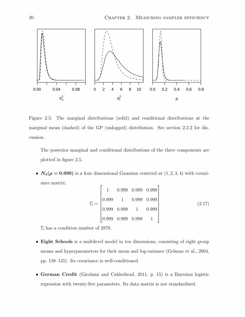
Figure 2.5: The marginal distributions (solid) and conditional distributions at the
marginal mean (dashed) of the GP (unlogged) distribution. See section 2.2.2 for dis-
cussion.
The posterior marginal and conditional distributions of the three components are
plotted in figure 2.5.
• N4(ρ = 0.999) is a four dimensional Gaussian centered at (1, 2, 3, 4) with covari-
ance matrix:
Σ =
1 0.999 0.999 0.999
0.999 1 0.999 0.999
0.999 0.999 1 0.999
0.999 0.999 0.999 1
(2.17)
Σ has a condition number of 2870.
• Eight Schools is a multilevel model in ten dimensions, consisting of eight group
means and hyperparameters for their mean and log-variance (Gelman et al., 2004,
pp. 138–145). Its covariance is well-conditioned.
• German Credit (Girolami and Calderhead, 2011, p. 15) is a Bayesian logistic
regression with twenty-five parameters. Its data matrix is not standardized.

2.2. Framework for comparing methods 21
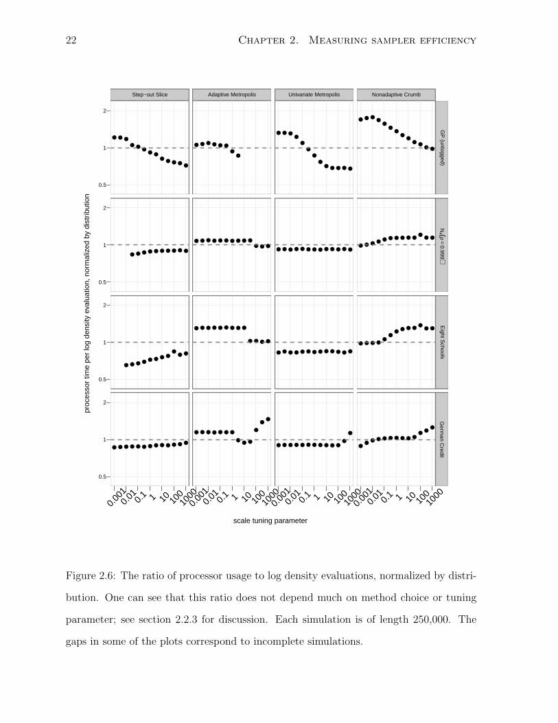
2.2.3 Processor time and log density evaluations
Before comparing performance of methods on a distribution, we must choose a mea-
sure of cost. Here, the methods of section 2.2.1 and distributions of section 2.2.2 are
used to justify the choice of log-density evaluations per MCMC iteration multiplied by
autocorrelation time.
If a user’s goal is to estimate a parameter to a specific accuracy, they would want
to choose an MCMC method that minimizes processor time per iteration multiplied by
autocorrelation time. However, processor time measurements made on a researcher’s
machine depend on idiosyncratic factors such as the type of machine the researcher is
using, other simultaneous tasks running on the machine, etc. Even identically configured
simulations may generate different results.
An alternative to measuring processor usage is counting log-density function evalu-
ations. Initialized with the same random seed, an MCMC simulation would evaluate
this function the same number of times on machines of different speeds, on the same
machine with different concurrent processes, and often even when implemented in dif-
ferent programming languages. However, this measure does not capture the overhead of
the MCMC method, nor does it capture different ways a distribution can be represented
to the method. For example, some methods require gradients to be computed, increas-
ing the processor time per evaluation; some methods, such as Gibbs sampling, do not
compute log densities at all.
To see the comparability of these two measures, at least on the distributions and
methods described in sections 2.2.1 and 2.2.2, see figure 2.6, which plots the ratio of
processor usage to log-density function evaluations for those samplers and distributions
and for a range of tuning parameters. The ratios are normalized to the median processor
time for a function evaluation over the simulations of that distribution. If processor usage
and log density evaluations were perfectly comparable, every plotted point would lie on
the dashed horizontal line indicating a ratio of one. For the simulations in figure 2.6, the
22 Chapter 2. Measuring sampler efficiency
scale tuning parameter
proc
esso
r tim
e pe
r lo
g de
nsity
eva
luat
ion,
nor
mal
ized
by
dist
ribut
ion
0.5
1
2
0.5
1
2
0.5
1
2
0.5
1
2
Step−out Slice
●●
● ●●
●
● ●● ● ● ● ●
●●●●●●●●●●
●●●
●●●●●●●●
●●●●●●●●●●●●●
0.00
10.
01 0.1 1 10 10
010
00
Adaptive Metropolis
● ● ● ● ● ●●
●
●●●●●●●●●●●●●
●●●●
●●●●●●●●●
●●
●
●●●
●●●●●●●
0.00
10.
01 0.1 1 10 10
010
00
Univariate Metropolis
● ● ●●
●●
●●
● ● ● ● ●
●●●●●●●●●●●●●
●●●●●●●●●●●●●
●
●●●●●●●●●●●●
0.00
10.
01 0.1 1 10 10
010
00
Nonadaptive Crumb
● ● ●●
●●
●●
●● ●
● ●
●●●
●●●●●●●●●●
●●●●●●●
●●
●●●●
●●●
●●●●●●●●●●
0.00
10.
01 0.1 1 10 10
010
00
GP
(unlogged)N
4 (ρ=
0.999)E
ight Schools
Germ
an Credit
Figure 2.6: The ratio of processor usage to log density evaluations, normalized by distri-
bution. One can see that this ratio does not depend much on method choice or tuning
parameter; see section 2.2.3 for discussion. Each simulation is of length 250,000. The
gaps in some of the plots correspond to incomplete simulations.
2.3. Graphical comparison of methods 23
measures are at most a small multiple off from each other. Even though the overhead of
Adaptive Metropolis, which is implemented in R and performs expensive matrix manipu-
lations, is much larger than that of Nonadaptive Crumb, which is implemented in C and
does not perform any expensive computations, the log density evaluations dominate the
cost. Because no significant differences in ratios are observed, I am inclined to believe
that comparing processor usage and comparing log density evaluations will yield similar
conclusions regarding the merits of various MCMC methods.
2.3 Graphical comparison of methods
The cost measure described in section 2.2.3, evaluations per uncorrelated observation,
provides a way of quantifying the performance of the MCMC methods described in sec-
tion 2.2.1 on the distributions described in section 2.2.2. I simulated each of these
distributions with each sampler for nine values of the sampler’s tuning parameter in the
range 0.001 to 1000. Each chain had a length of 250,000. Treating the first half of each
chain as a burn-in period, I computed the autocorrelation time of each simulation using
the AR process method of section 2.1.4 and multiplied it by the average number of log
density evaluations the simulation needed per iteration to generate an estimate of the
number of log density evaluations per uncorrelated observation. Smaller values indicate
better performance. In this section and subsequent ones, I use the true mean instead of
the sample mean when estimating autocorrelation times to reduce the chance that an er-
roneously low autocorrelation time will be estimated if a chain appears to have converged
but has not.
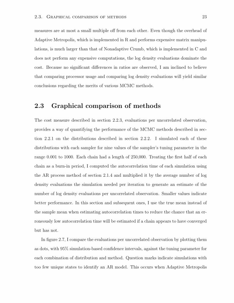
In figure 2.7, I compare the evaluations per uncorrelated observation by plotting them
as dots, with 95% simulation-based confidence intervals, against the tuning parameter for
each combination of distribution and method. Question marks indicate simulations with
too few unique states to identify an AR model. This occurs when Adaptive Metropolis
24 Chapter 2. Measuring sampler efficiency
scale tuning parameter
# of
eva
ls. o
f log
den
sity
func
tion
per
unco
rrel
ated
obs
. (w
ith 9
5% C
I)
102
103
104
105
106
107
102
103
104
105
106
107
102
103
104
105
106
107
102
103
104
105
106
107
Step−out Slice
●●
●
●●
●
● ● ● ● ● ● ●
●●●●●●●●
●●
???
●●●●●●
●
●
●●
●
??
●●●●●●●●●
●
●●
●
0.00
10.
01 0.1 1 10 10
010
00
Adaptive Metropolis
● ● ● ● ●● ● ●
?????
●
●●●●●●●●
●
???
●●●●
●●
●●
●
????
●●
●
●
●●●
??????
0.00
10.
01 0.1 1 10 10
010
00
Univariate Metropolis
● ● ●●
●● ● ●
● ●
●●
●
●●●●●
●●●
●●
●●●
●●
●●
●●
●
●
●
●●●●
●●●●●●
●●●
●
●
●●
0.00
10.
01 0.1 1 10 10
010
00
Nonadaptive Crumb
● ● ● ● ● ● ● ● ● ● ● ● ●
●●●●●●●●●●
●●●
●●●●●●●●
●
●
●●●
●●●●●●●
●●●●●●
0.00
10.
01 0.1 1 10 10
010
00
GP
(unlogged)N
4 (ρ=
0.999)E
ight Schools
Germ
an Credit
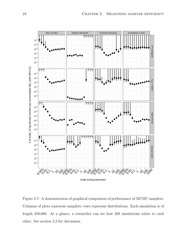
Figure 2.7: A demonstration of graphical comparison of performance of MCMC samplers.
Columns of plots represent samplers; rows represent distributions. Each simulation is of
length 250,000. At a glance, a researcher can see how 208 simulations relate to each
other. See section 2.3 for discussion.

2.3. Graphical comparison of methods 25
has a near-100% rejection rate and when Step-out Slice is badly enough tuned that the
test framework aborts the simulation.
2.3.1 Between-cell comparisons
Scanning an individual cell in the grid of plots, one can see how performance varies
with the tuning parameter. Scanning down columns of the grid of plots, one can see
how performance varies from distribution to distribution for a given MCMC method.
Scanning across rows of the grid of plots, one can see how performance varies from
method to method for a given distribution.
Doing this, several patterns emerge. For example, one can see that Adaptive Metropo-
lis performs consistently well for a variety of tuning parameters, as long as the tuning
parameter is smaller than the square root of the smallest eigenvalue of the distribution’s
covariance. Either it performs well or does not converge at all. This suggests that Adap-
tive Metropolis users uncertain about the distribution they are sampling from should err
in the direction of small tuning parameters.
A second pattern is that Univariate Metropolis tends to have U-shaped comparison
plots. Tuning parameters that are either too small or too large lead to unacceptable
performance. And, the lowest points on these plots are still usually above the flat parts
of the Adaptive Metropolis plots. On low-dimensional distributions like these, where the
sampler does not know the structure of the target density, Adaptive Metropolis can be
considered to dominate Univariate Metropolis.
Reading across rows, one can see different sorts of patterns. For example, The GP
(unlogged) and N4(ρ = 0.999) rows are flat within cells, but not between them, suggesting
that for those distributions, one needs to pay more attention to the choice of method
than its tuning.
26 Chapter 2. Measuring sampler efficiency
2.3.2 Within-cell comparisons
A different sort of pattern can be seen in the slopes of the lines traced out by the
plot symbols. For Univariate Metropolis on GP (unlogged), Eight Schools, and German
Credit, for tuning parameters less than one, a decrease in the tuning parameter by a
factor of ten leads to a factor of almost one hundred degraded performance—a slope
of −2 in the log domain. For these tuning parameters, the Markov chains are nearly
a random walk. Such a random walk will travel some distance in a number of steps
proportional to the square of that distance (Feller, 1968, p. 90).
This contrasts with the slope of the plot symbols for Step-out Slice, which is close
to −1 for small tuning parameters on the same distributions. Step-out Slice requires a
number of log density function evaluations linear in the ratio of slice width to tuning
parameter to determine an initial slice estimate, so decreasing the tuning parameter by
some factor degrades the performance by that factor.
A pattern in the slopes for large parameters can be seen with Univariate Metropolis on
Eight Schools with tuning parameters larger than one. In those simulations, multiplying
the tuning parameter by ten degrades performance by a factor of approximately ten—a
slope of one in the log domain. Increasing the tuning parameter by some factor reduces
the acceptance rate by approximately that factor when the tuning parameter is large.
This behavior contrasts with the two slice samplers, whose costs trace logarithmic
curves for large tuning parameters on N4(ρ = 0.999) and German Credit. On average,
each rejected proposal reduces the estimated slice size by a constant factor, so an increase
in a tuning parameter above the optimal value by some factor increases the computation
cost by the log of that factor.
None of the patterns of this section would be easily visible if the results were presented
in tabular form. Figure 2.7 shows summaries of 208 simulations, more than could be
absorbed by a reader if presented as text.
2.3. Graphical comparison of methods 27
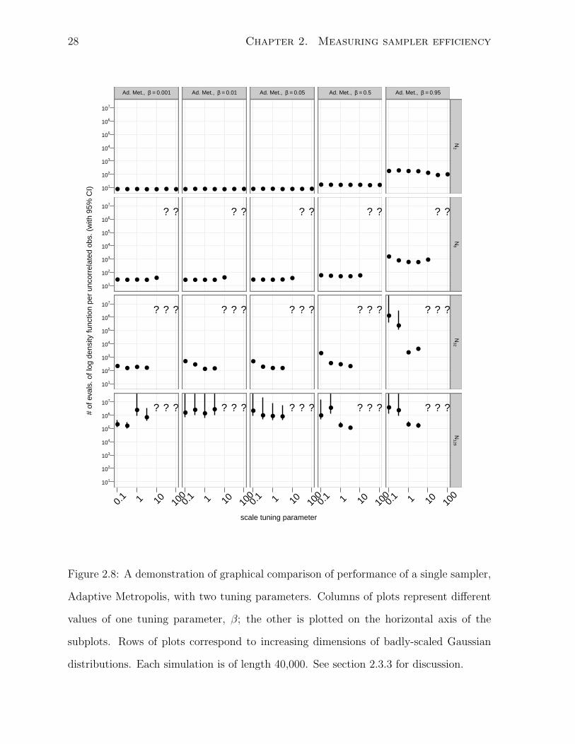
2.3.3 Comparison with multiple tuning parameters
While plots like figure 2.7 allow a broad comparison of distributions and methods, it is
often necessary to compare different sets of factors. The same type of plot can be used
when varying extra parameters associated with either the distribution or the MCMC
method. Figure 2.8 is an example of such a comparison. It focuses just on Adaptive
Metropolis sampling from badly-scaled Gaussians.
One tuning parameter of Adaptive Metropolis is β, the fraction of proposals drawn
from a spherical Gaussian instead of a Gaussian with a learned covariance. Roberts and
Rosenthal (2009) suggest the value of 0.05. In this example, I vary it from 0.001 to 0.95.
At the same time, I consider the effect of dimensionality on the performance of the
method. Each target distribution is a multivariate Gaussian with uncorrelated compo-
nents. The variance is equal to 1000 in one coordinate and one in the rest. The problem
dimension ranges from 2 to 128. While the high-variance component is axis-aligned,
this does not affect the results because the behavior of Adaptive Metropolis is invariant
to rotations of the target distribution. As with the simulations of figure 2.7, Adaptive
Metropolis performs well when the principal tuning parameter is smaller than the square
root of the smallest eigenvalue of the target distribution’s covariance, in this case one.
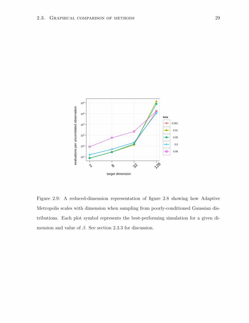
Having seen this pattern, it is useful to summarize the comparisons by choosing the
lowest-cost simulation from each grid cell and plotting them in a single graph, as in
figure 2.9. In both figure 2.8 and figure 2.9, one can see that while Adaptive Metropolis
performs better in low dimensional spaces, this performance does not vary much with β
in any of the dimensions simulated.
2.3.4 Discussion of graphical comparison
Section 2.3 shows the variation in performance of MCMC methods while varying method,
distribution, and one tuning parameter as well as the variation in performance of a single
28 Chapter 2. Measuring sampler efficiency
scale tuning parameter
# of
eva
ls. o
f log
den
sity
func
tion
per
unco
rrel
ated
obs
. (w
ith 9
5% C
I) 101
102
103
104
105
106
107
101
102
103
104
105
106
107
101
102
103
104
105
106
107
101
102
103
104
105
106
107
Ad. Met., β = 0.001
● ● ● ● ● ● ●
● ● ● ● ●
? ?
● ● ● ●
? ? ?
● ●
●
●
? ? ?
0.1 1 10 10
0
Ad. Met., β = 0.01
● ● ● ● ● ● ●
● ● ● ● ●
? ?
●●
● ●
? ? ?
●●
●● ? ? ?
0.1 1 10 10
0
Ad. Met., β = 0.05
● ● ● ● ● ● ●
● ● ● ● ●
? ?
●● ● ●
? ? ?
●● ● ●
? ? ?
0.1 1 10 10
0
Ad. Met., β = 0.5
● ● ● ● ● ● ●
● ● ● ● ●
? ?
●
● ● ●
? ? ?
●
●
● ●
? ? ?
0.1 1 10 10
0
Ad. Met., β = 0.95
● ● ● ● ● ● ●
●● ● ● ●
? ?
●
●
●●
? ? ?
●●
● ●
? ? ?
0.1 1 10 10
0
N2
N8
N32
N128
Figure 2.8: A demonstration of graphical comparison of performance of a single sampler,
Adaptive Metropolis, with two tuning parameters. Columns of plots represent different
values of one tuning parameter, β; the other is plotted on the horizontal axis of the
subplots. Rows of plots correspond to increasing dimensions of badly-scaled Gaussian
distributions. Each simulation is of length 40,000. See section 2.3.3 for discussion.
2.3. Graphical comparison of methods 29
target dimension
eval
uatio
ns p
er u
ncor
rela
ted
obse
rvat
ion
101
102
103
104
105
106
●
●
●
●
2 8 32 128
beta
● 0.001
0.01
0.05
0.5
0.95
Figure 2.9: A reduced-dimension representation of figure 2.8 showing how Adaptive
Metropolis scales with dimension when sampling from poorly-conditioned Gaussian dis-
tributions. Each plot symbol represents the best-performing simulation for a given di-
mension and value of β. See section 2.3.3 for discussion.

30 Chapter 2. Measuring sampler efficiency
MCMC method while varying two tuning parameters and the dimension of the target
distribution. In general, one may use the plots described in this section to compare
performance of MCMC methods while varying any three factors. Comparing performance
with tabulated summary statistics, in contrast, only allows researchers to study variation
in one factor at once, a significant disadvantage.
One might wonder, then, how one could visualize performance as more than three
factors vary simultaneously. While it may be useful, computational limits become an
obstacle as the number of parameters increases. Figure 2.7 compares 208 simulations.
Even if there were a clear way to visualize cost as four or five factors vary, one would need
to run thousands of simulations to make such a plot. The plots of this section display
approximately as much information as is currently feasible to gather.
Other variations on these plots are possible, such as the one used for figure 2.9. One
variant not shown replaces confidence intervals by multiple plot symbols, each represent-
ing a replication of the same simulation with a different random seed. Multiple symbols
are plotted in a column for a given tuning parameter. Making the symbols partially
transparent makes such a graph easier to read.
If one is willing to forego all measures of uncertainty under replication, one can omit
the confidence intervals and plot figures of merit for multiple values of a second factor,
such as a second tuning parameter, in a single grid cell, differentiating levels of this factor
by color or plot symbol. However, this technique can produce confusing graphs if the
factor represented by color or plot symbol is not naturally nested in the factor represented
by columns of plots—one should not vary a factor like problem dimension inside a single
grid cell.
Chapter 3
Samplers with multivariate steps
This chapter presents several new variations of slice sampling. First, it gives background
on slice sampling with multivariate steps. Then, it presents several globally-adaptive
eigendecomposition-based methods and several locally-adaptive gradient-based methods
in the crumb framework. Finally, it compares the methods using the scheme described
in chapter 2.
3.1 Slice sampling overview
Slice sampling is a robust Markov chain Monte Carlo method in which a new state
is drawn from a “slice” containing all points whose density is larger than an auxiliary
variable, y. Uniformly sampling from the volume under a probability density function,
f(·), gives a sample {(xi, yi)}, where xi ∈ Rp and yi ∈ R+. The marginal distribution of
xi then has density f(xi). So, if one can devise a way of sampling uniformly from the
volume underneath a distribution’s density curve, one can convert this to a method for
sampling from the distribution itself by dropping the yi from the resulting sample.
Slice sampling accomplishes this by alternating steps that update the y coordinate
and steps that update the x coordinates. Updating the y coordinate is easy: the con-
ditional distribution for yi+1 given xi is uniform on the interval [0, f(xi)]. Updating the
31
32 Chapter 3. Samplers with multivariate steps
x coordinate is more difficult, in general, so instead of updating xi with its conditional
distribution, general purpose slice samplers perform a state transition that leaves the
conditional distribution given yi invariant. An update to xi seeks an xi+1 such that if
xi is uniformly distributed on the current slice through the density, {x|f(x) ≥ yi}, then
xi+1 will also be uniformly distributed on the same slice. Neal (2003) discusses various
methods that satisfy this condition. This chapter and chapter 4 extend his work, focusing
on adaptive multivariate updates.
The methods described in this document evaluate the log density function of the target
distribution, usually denoted by `(·), rather than the density function itself, because
working in the log domain makes numeric underflow and overflow less likely. Let E
have an exponential distribution with mean one. The value exp(−E) has a uniform
distribution, so instead of using a uniform draw on [0, f(x)] as the slice level, we can use
`(x)− E as a log-domain slice level:
exp(`(x)− E) = f(x) · exp(−E), where E ∼ Exponential(1) (3.1)
= f(x) · U, where U ∼ Uniform[0, 1] (3.2)
∼ Uniform[0, f(x)] (3.3)
This way, we never need to compute exp `(x), which can overflow or underflow.
3.2 Methods based on eigenvector decomposition
In this section, the approach to adaptive MCMC that Haario et al. (2001) use to improve
random-walk Metropolis is applied to improve two variations on slice sampling. These
methods continuously adapt, learning the global structure of the distribution as they
move through the state space. They converge asymptotically to the target distribution,
but do not have a fixed stationary distribution, so they can be difficult to analyze for
convergence. They can also be difficult to embed in a larger sampling scheme because
3.2. Methods based on eigenvector decomposition 33
their adapted state may become inappropriate when the variables the target distribution
conditions on change.
When components of the target distribution are highly correlated, the Markov chains
generated by slice samplers that make univariate updates (Neal, 2003, §4) will mix slowly.
If two components are highly correlated, the contours of the target density will not be
axis-aligned, so univariate slice updates with stepping out or doubling will always take
steps across short, axis-aligned cuts through these contours. The hyperrectangle method
(Neal, 2003, §5.1) is a slice sampling variant that takes multivariate steps by drawing
proposals from an axis-aligned hyperrectangle positioned randomly with respect to the
current point. It is unlikely to accept a proposal until the hyperrectangle has edges of
length comparable to the shortest diameter of the log density contour that defines the
current slice. Therefore, it behaves similarly to methods that take univariate updates
when the components of the target distribution are highly correlated.
We must somehow take steps in non-axis-aligned directions for the Markov chain
to mix quickly on distributions where components of the target distribution are highly
correlated. If the target distribution is Gaussian, the contours are concentric ellipsoids. If
the log density of the target distribution is convex and not highly skewed, the contours are
at least roughly ellipsoidal. We can create an ellipsoidal approximation to a slice contour
by aligning the axes of an ellipsoid with the eigenvectors of the sample covariance matrix
and choosing the axis lengths to be proportional to the square roots of the corresponding
eigenvalues. Unless the log density is unimodal and normalized, it is difficult to compute
the optimal proportionality constant. (This issue is discussed in section 4.1.2.)
This idea motivates two variations on slice sampling that use an approximation to
the covariance matrix of the target distribution. One approach is to take univariate steps
with stepping out in the coordinate space defined by the eigenvectors, with initial slice
widths proportional to the square roots of the corresponding eigenvalues. This method
is discussed in section 3.2.1.
34 Chapter 3. Samplers with multivariate steps
The second approach is an extension of the hyperrectangle method. The hyperrect-
angle method can be modified so that the axes of the initial hyperrectangles are oriented
along eigenvectors, and the lengths of the sides of the initial hyperrectangle are propor-
tional to the square roots of the eigenvalues. This method is discussed in section 3.2.3.
Both methods require an approximation of the covariance matrix. Haario et al. (2001)
show that one can use a mixture of spherically symmetric Gaussian proposals and the
sample covariance matrix to generate an adaptive Metropolis proposal distribution. Using
a theorem from Roberts and Rosenthal (2007), they show that the resulting Markov chain
converges to the intended distribution. Section 3.2.5 uses a similar argument to show
that the modified hyperrectangle method converges to the intended distribution.
3.2.1 Univariate updates along eigenvectors
“Univar Eigen,” inspired by Tibbits et al. (2010), is a variation of slice sampling that
makes univariate updates along the eigenvectors of the sample covariance matrix. If the
log density of the target distribution is approximately convex, so that there is not radical
variation in the shape of the target distribution from point to point, the contours of the
distribution will be approximately ellipsoidal and the eigenvectors of its covariance will
roughly coincide with the axes of these ellipsoids. Steps taken along the eigenvectors,
therefore, will include steps along the long axes of a slice even when the axes of the
contours do not coincide with the coordinate axes.
Computing these directions requires an estimate of the covariance. Tibbits et al. use
the sample covariance from a trial run to estimate the full covariance matrix of the
hyperparameters and the marginal variances of the remaining parameters. Univar Eigen
instead uses the full sample covariance matrix of the current chain, as done by Haario
et al. (2001) in Adaptive Metropolis. Like Adaptive Metropolis, Univar Eigen takes a
small fraction of its steps from a fixed distribution to avoid becoming trapped in a bad
adaptive state. It has two tuning parameters: β, the proportion of iterations that use
3.2. Methods based on eigenvector decomposition 35
non-adapted steps, and w, the initial segment length for non-adapted steps. β is usually
fixed at 0.05, as in Adaptive Metropolis.
Suppose our Markov chain has taken n steps, generating a sequence of dependent
p-vector-valued random variables (X1, . . . , Xn) from the target distribution. Denote the
sample covariance of this sequence by Sn. Denote the eigenvectors of Sn by (v1, . . . , vp)
and the eigenvalues of Sn by (λ1, . . . , λp). Each iteration, Univar Eigen chooses a random
number U ∈ [0, 1]. If U < β or n < p (making Sn rank-deficient), the initial slice
approximation is a segment of length w in a random direction placed so that the offset
of the current state, Xn, from the end of the segment is uniformly distributed on [0, w].
If U ≥ β, an eigenvector-eigenvalue pair (vi, λi) is chosen, with i uniformly drawn from
{1, . . . , p}. The initial slice proposal is then a segment of length√λi in the direction vi
placed so that the offset of the current state from the end of the segment is uniformly
distributed on[0,√λi].
The initial segment can be expanded by stepping out as discussed in Neal (2003, §4),
but this is not strictly necessary since using an eigenvalue to compute the initial slice
approximation leads to reasonable scaling. However, stepping out does lead to greater
robustness and has minimal downside. It is used in the experiments of section 3.2.2,
but the results are similar if it is not. Once an initial slice approximation is chosen, a
proposal for Xn+1 is drawn uniformly from the segment. If the proposed step is outside
the slice, it is rejected and the segment is shrunk so that the next proposal is drawn from
the portion of the segment on the same side of the rejected proposal as Xn. Proposals
are drawn and the approximation shrunk until a proposal is accepted.
When the target distribution is p-dimensional, the computation of the eigendecom-
position of Sn is O(p3), so it is not done every iteration. In the implementation evaluated
here, the number of decomposition updates is limited to one hundred. For example, on a
chain length of 50,000, the eigendecomposition will be updated every 500 iterations. Only
one in every p univariate updates is used to update the scatter matrix used to compute
36 Chapter 3. Samplers with multivariate steps
Sn, and each update takes O(p2) operations. Since an individual one-dimensional up-
date takes O(p) operations, neither the cost of updating the eigendecomposition nor the
cost of maintaining the scatter matrix is dominant for long chains or in high-dimensional
spaces.
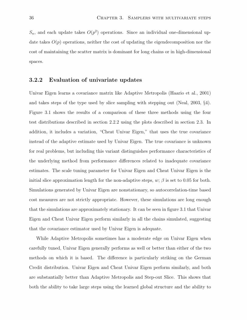
3.2.2 Evaluation of univariate updates
Univar Eigen learns a covariance matrix like Adaptive Metropolis (Haario et al., 2001)
and takes steps of the type used by slice sampling with stepping out (Neal, 2003, §4).
Figure 3.1 shows the results of a comparison of these three methods using the four
test distributions described in section 2.2.2 using the plots described in section 2.3. In
addition, it includes a variation, “Cheat Univar Eigen,” that uses the true covariance
instead of the adaptive estimate used by Univar Eigen. The true covariance is unknown
for real problems, but including this variant distinguishes performance characteristics of
the underlying method from performance differences related to inadequate covariance
estimates. The scale tuning parameter for Univar Eigen and Cheat Univar Eigen is the
initial slice approximation length for the non-adaptive steps, w; β is set to 0.05 for both.
Simulations generated by Univar Eigen are nonstationary, so autocorrelation-time based
cost measures are not strictly appropriate. However, these simulations are long enough
that the simulations are approximately stationary. It can be seen in figure 3.1 that Univar
Eigen and Cheat Univar Eigen perform similarly in all the chains simulated, suggesting
that the covariance estimator used by Univar Eigen is adequate.
While Adaptive Metropolis sometimes has a moderate edge on Univar Eigen when
carefully tuned, Univar Eigen generally performs as well or better than either of the two
methods on which it is based. The difference is particularly striking on the German
Credit distribution. Univar Eigen and Cheat Univar Eigen perform similarly, and both
are substantially better than Adaptive Metropolis and Step-out Slice. This shows that
both the ability to take large steps using the learned global structure and the ability to
3.2. Methods based on eigenvector decomposition 37
scale tuning parameter
# of
eva
ls. o
f log
den
sity
func
tion
per
unco
rrel
ated
obs
. (w
ith 9
5% C
I)
102
103
104
105
106
107
102
103
104
105
106
107
102
103
104
105
106
107
102
103
104
105
106
107
Step−out Slice
●●
●
●●
●
● ● ● ● ● ● ●
●●●●●●●●
●●
???
●●●●●●
●
●
●●
●
??
●●●●●●●●●
●
●●
●
0.00
10.
01 0.1 1 10 10
010
00
Adaptive Metropolis
● ● ● ● ●● ● ●
?????
●
●●●●●●●●
●
???
●●●●
●●
●●
●
????
●●
●
●
●●●
??????
0.00
10.
01 0.1 1 10 10
010
00
Univar Eigen
● ● ● ● ●● ● ● ● ●
●● ●
● ● ● ● ● ● ● ● ● ● ● ● ●
● ● ● ● ●● ● ● ●
● ● ● ●
●
● ● ● ●●
●● ●
●
● ● ●
0.00
10.
01 0.1 1 10 10
010
00
Cheat Univar Eigen
● ● ● ● ● ● ● ● ● ● ● ● ●
● ● ● ● ● ● ● ● ● ● ● ● ●
● ● ● ● ● ● ● ●● ● ● ● ●
● ● ● ● ● ● ● ● ● ● ● ● ●
0.00
10.
01 0.1 1 10 10
010
00
GP
(unlogged)N
4 (ρ=
0.999)E
ight Schools
Germ
an Credit
Figure 3.1: A comparison of Univar Eigen to two other MCMC methods using simulations
of length 50,000. Question marks indicate simulations that were aborted or trapped in a
single state. See section 3.2.2 for discussion.
38 Chapter 3. Samplers with multivariate steps
take small steps when the local structure differs from the global structure contribute to
fast mixing.
Because of the promise shown by Univar Eigen in this section, it is included in a
broader comparison of methods in section 3.6.
3.2.3 Multivariate updates with oblique hyperrectangles
Section 3.2.1 extends slice sampling with stepping out to use a coordinate system based
on the covariance of the target distribution; this section similarly extends the hyper-
rectangle method (Neal, 2003, §5.1), which takes multivariate steps in a slice using a
hyperrectangular initial slice approximation.
In each iteration of Neal’s hyperrectangle method, an axis-aligned hypercube approxi-
mating the slice is placed randomly so that the distribution of the current state is uniform
relative to the hypercube. A proposal is then drawn from the hypercube; if it is inside the
slice, it is accepted. Since the distributions of the current state and the proposal are the
same relative to the hypercube, the stationary distribution is invariant. If the proposal
is not in the slice, just as a segment is shrunk towards the current state when sampling
with univariate updates, the hypercube is divided in two by the hyperplane through the
rejected proposal and normal to the coordinate direction in which the gradient of the log
density is largest, and the section of the hypercube not containing the current state is
removed from the approximation. Then, a new proposal is drawn, a new section of the
hyperrectangle is removed if this proposal is not in the slice, and so on until a proposal
is inside the slice. If gradients are not available, instead of only shrinking one coordi-
nate, every coordinate is shrunk towards the initial state, leaving the rejected proposal
as a corner of the updated hyperrectangular slice approximation. (Figure 3.3 on page 45
includes a graphical example of these updates.)
If gradients are available, efficient sampling is possible on distributions whose compo-
nents have greatly unequal variances but little correlation. If gradients are not available,
3.2. Methods based on eigenvector decomposition 39
efficient sampling is only possible on distributions whose coordinates are uncorrelated
and have similar variances because a proposal will only be accepted when the slice ap-
proximation has edge sizes comparable to the least variable coordinate.
Here, I present an alternative hyperrectangle method that uses an approach similar
to that of section 3.2.1. It orients the initial hyperrectangle so that its edges are parallel
to the eigenvectors of the sample covariance and have lengths proportional to the square
roots of the eigenvalues of the sample covariance. Since the approximation is hopefully
properly scaled and aligned with the contours, when a proposal is rejected, it is reasonable
to assume that the estimate is too large in all directions and that gradients are not
necessary to pick a direction in which to shrink the approximation.
This method has two tuning parameters, β and w, similar to the parameters with the
same names in section 3.2.1. An iteration begins by creating an initial hyperrectangular
slice approximation. With probability β, the initial hyperrectangle is a unit hypercube
with edge length 5w and axes aligned with the coordinate axes. Otherwise, axis i (for
i ∈ (1, . . . , p)) has length 5√λi and orientation vi. In either case, the hyperrectangle
is positioned so that the offset of the current state, Xn, from a corner of the initial
hyperrectangle has a uniform distribution.
A proposal is drawn uniformly from the hyperrectangle, and the log density at the
proposal is evaluated. If the log density is greater than or equal to the slice level, the
proposal is accepted. Otherwise, it is rejected, and the hyperrectangle is shrunk without
changing the orientation of its axes so that the rejected proposal is a corner of the
hyperrectangular slice approximation and the current state remains in the interior of
the hyperrectangle. Proposals are drawn, and the slice approximation is shrunk, until
a proposal is accepted. This procedure is identical to the procedure described by Neal
except in the way that the initial hyperrectangle is chosen.
Empirically, the performance of the method does not depend much on the propor-
tionality constant for the edge lengths, five. If the constant is at least one, the slice
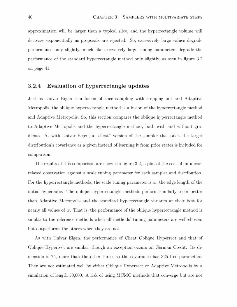
40 Chapter 3. Samplers with multivariate steps
approximation will be larger than a typical slice, and the hyperrectangle volume will
decrease exponentially as proposals are rejected. So, excessively large values degrade
performance only slightly, much like excessively large tuning parameters degrade the
performance of the standard hyperrectangle method only slightly, as seen in figure 3.2
on page 41.
3.2.4 Evaluation of hyperrectangle updates
Just as Univar Eigen is a fusion of slice sampling with stepping out and Adaptive
Metropolis, the oblique hyperrectangle method is a fusion of the hyperrectangle method
and Adaptive Metropolis. So, this section compares the oblique hyperrectangle method
to Adaptive Metropolis and the hyperrectangle method, both with and without gra-
dients. As with Univar Eigen, a “cheat” version of the sampler that takes the target
distribution’s covariance as a given instead of learning it from prior states is included for
comparison.
The results of this comparison are shown in figure 3.2, a plot of the cost of an uncor-
related observation against a scale tuning parameter for each sampler and distribution.
For the hyperrectangle methods, the scale tuning parameter is w, the edge length of the
initial hypercube. The oblique hyperrectangle methods perform similarly to or better
than Adaptive Metropolis and the standard hyperrectangle variants at their best for
nearly all values of w. That is, the performance of the oblique hyperrectangle method is
similar to the reference methods when all methods’ tuning parameters are well-chosen,
but outperforms the others when they are not.
As with Univar Eigen, the performance of Cheat Oblique Hyperrect and that of
Oblique Hyperrect are similar, though an exception occurs on German Credit. Its di-
mension is 25, more than the other three, so the covariance has 325 free parameters.
They are not estimated well by either Oblique Hyperrect or Adaptive Metropolis by a
simulation of length 50,000. A risk of using MCMC methods that converge but are not
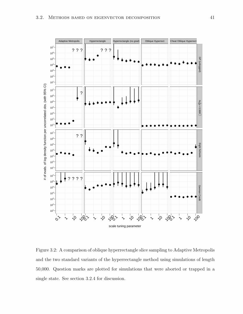
3.2. Methods based on eigenvector decomposition 41
scale tuning parameter
# of
eva
ls. o
f log
den
sity
func
tion
per
unco
rrel
ated
obs
. (w
ith 9
5% C
I)
101
102
103
104
105
106
107
101
102
103
104
105
106
107
101
102
103
104
105
106
107
101
102
103
104
105
106
107
Adaptive Metropolis
●● ● ●
? ? ?
●
●●●●●
?
●●●●
●
??
●
●●
????
0.1 1 10 10
0
Hyperrectangle
● ● ●
●
? ? ?
● ● ● ● ● ● ●
●
● ●●
●
● ●
●●
●● ●
● ●
0.1 1 10 10
0
Hyperrectangle (no grad)
●●
● ● ● ● ●
●
●
● ●● ●
●
●●
●● ●
● ●
●●
●● ●
● ●
0.1 1 10 10
0
Oblique Hyperrect
● ● ● ● ● ● ●
● ● ● ● ● ● ●
● ● ●● ●
● ●
●
● ●●
● ●●
0.1 1 10 10
0
Cheat Oblique Hyperrect
● ● ●● ● ● ●
● ● ● ● ● ● ●
●● ●
● ●●
●
● ● ● ● ● ● ●
0.1 1 10 10
0
GP
(unlogged)N
4 (ρ=
0.999)E
ight Schools
Germ
an Credit
Figure 3.2: A comparison of oblique hyperrectangle slice sampling to Adaptive Metropolis
and the two standard variants of the hyperrectangle method using simulations of length
50,000. Question marks are plotted for simulations that were aborted or trapped in a
single state. See section 3.2.4 for discussion.
42 Chapter 3. Samplers with multivariate steps
stationary is that diagnostic summaries are dependent on the simulation length.
Like Univar Eigen, Oblique Hyperrect shows potential and is included in a broader
comparison of methods in section 3.6.
3.2.5 Convergence of the oblique hyperrectangle method
In this section, I use a theorem of Roberts and Rosenthal to show that the distribution of
the observations generated by the oblique hyperrectangle method converges to the target
distribution in the total variation norm as a consequence of its diminishing adaptation
when it is used to sample from distributions with connected, compact support. The
support of the target distribution must be connected because otherwise, even the non-
adaptive hyperrectangle method might not converge to the target distribution.
Roberts and Rosenthal (2007) show that several sets of conditions are sufficient for an
adaptive MCMC method to converge to the target distribution. All of these conditions
include “diminishing adaptation,” defined as:
supx‖PΓn+1(x, ·)− PΓn(x, ·)‖TV → 0 in probability as n→∞ (3.4)
Here, PΓn(x, ·) is the transition density at iteration n with “adaptation state” Γn and
current state x. The norm, ‖ · ‖TV, is the total variation norm. For the oblique hyper-
rectangle method, the adaptation state is the sample covariance, which encapsulates all
non-constant aspects of the transition density at a particular iteration.
When computing the sample covariance matrix, each iteration has weight 1/n. Since
oblique hyperrectangle transitions are bounded by the initial hyperrectangle, the most
extreme transition can only move a finite distance from the center of the hyperrectangle.
The relative change in the ith eigenvalue between steps n and n + 1 is O(1/n) since
the maximum step size in the direction of the corresponding eigenvector is proportional
to the square root of that eigenvalue. The same holds for updates to the eigenvectors:
the eigenvectors of Γn+1 are a mixture of the eigenvectors of Γn and the observation at
3.2. Methods based on eigenvector decomposition 43
iteration n, where the total weight given to the observation at iteration n over all the
directions is O(1/n). Since each eigenvalue can change by O(1/n) and each eigenvec-
tor can rotate by an angle O(1/n), each initial hyperrectangle diameter can change by
O(1/√n). Conditioning on the random draw that positions the initial hyperrectangles
with respect to the current state, the ratio of the volume occupied by the symmetric
difference between the hyperrectangles for states Γn and Γn+1 to the volume of either
hyperrectangle is O(1/√n). Therefore, the probability of a proposal falling inside one
hyperrectangle and not another is O(1/√n); the difference in densities for proposals
falling inside both is also O(1/√n). Consequently, the total variation distance between
PΓn(x, ·) and PΓn+1(x, ·) is O(1/√n), where the proportionality constant does not depend
on x, so the diminishing adaptation condition is satisfied. Golub and Van Loan (1996,
pp. 395–397) discuss changes in eigendecompositions after rank-one updates in greater
detail.
If the target distribution has compact, connected support, the non-adaptive hyper-
rectangle method converges to the target distribution for any initial state and any full-
rank initial hyperrectangle orientation and dimensions. Let the space of adaptive states
be the set of all positive definite covariance matrices with all eigenvalues no smaller than
some positive lower bound. Because the maximum eigenvalue of the covariance matrices
is limited by the the boundedness of the support of the target distribution, this space
is compact with respect to the Euclidean norm. The probability mass in the difference
between two full-rank initial hyperrectangles in a neighborhood of γ will shrink to zero
as the size of the neighborhood approaches zero, so the mapping (x, γ) 7→ Pγ(x, ·) is con-
tinuous with respect to the total variation norm. By lemma 1 of Roberts and Rosenthal
(2007), this implies that the mapping (x, γ) 7→ ‖P nγ (x, ·) − f(·)‖TV is also continuous.
This continuity, along with diminishing adaptation and the convergence of P nγ (x, ·) to
f(·) for each individual x and γ, imply, by corollary 3 of Roberts and Rosenthal (2007),
that the adaptive hyperrectangle method converges to the target distribution in total
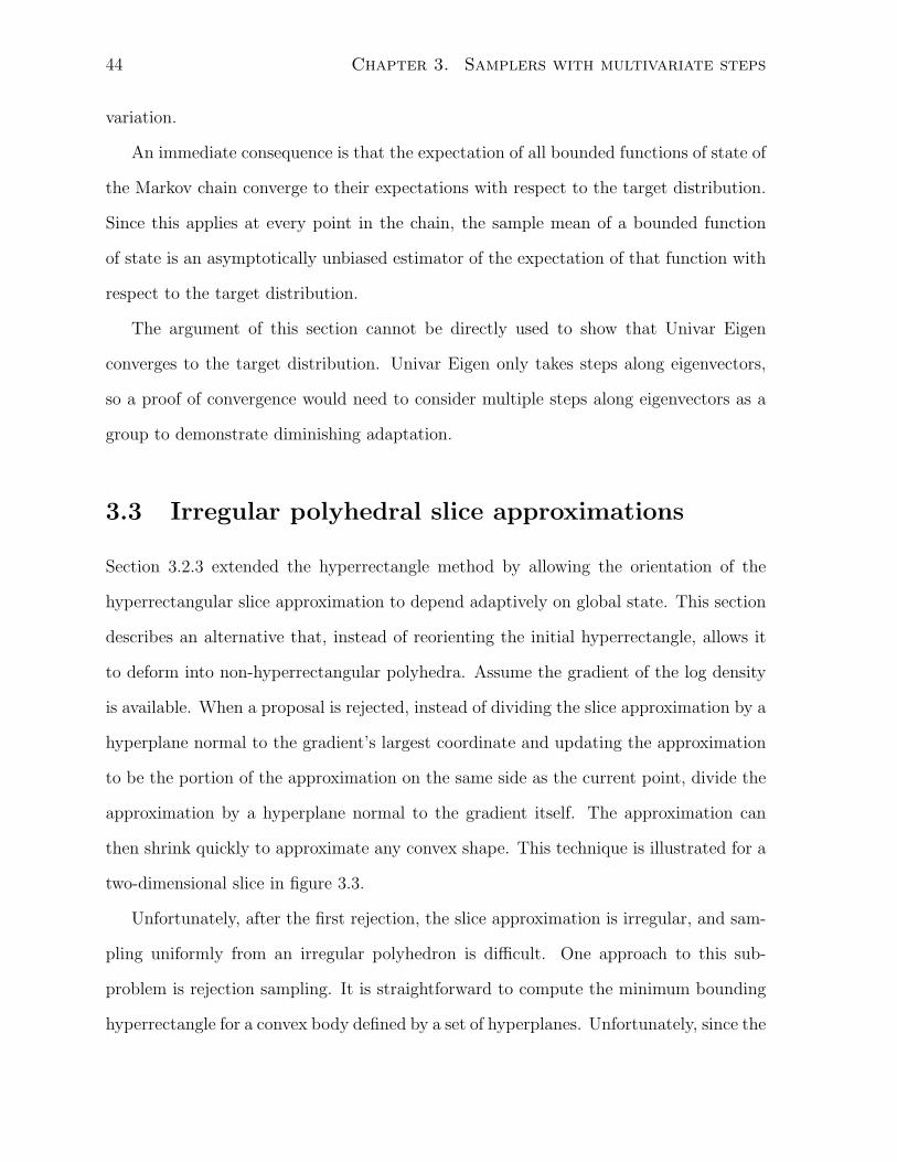
44 Chapter 3. Samplers with multivariate steps
variation.
An immediate consequence is that the expectation of all bounded functions of state of
the Markov chain converge to their expectations with respect to the target distribution.
Since this applies at every point in the chain, the sample mean of a bounded function
of state is an asymptotically unbiased estimator of the expectation of that function with
respect to the target distribution.
The argument of this section cannot be directly used to show that Univar Eigen
converges to the target distribution. Univar Eigen only takes steps along eigenvectors,
so a proof of convergence would need to consider multiple steps along eigenvectors as a
group to demonstrate diminishing adaptation.
3.3 Irregular polyhedral slice approximations
Section 3.2.3 extended the hyperrectangle method by allowing the orientation of the
hyperrectangular slice approximation to depend adaptively on global state. This section
describes an alternative that, instead of reorienting the initial hyperrectangle, allows it
to deform into non-hyperrectangular polyhedra. Assume the gradient of the log density
is available. When a proposal is rejected, instead of dividing the slice approximation by a
hyperplane normal to the gradient’s largest coordinate and updating the approximation
to be the portion of the approximation on the same side as the current point, divide the
approximation by a hyperplane normal to the gradient itself. The approximation can
then shrink quickly to approximate any convex shape. This technique is illustrated for a
two-dimensional slice in figure 3.3.
Unfortunately, after the first rejection, the slice approximation is irregular, and sam-
pling uniformly from an irregular polyhedron is difficult. One approach to this sub-
problem is rejection sampling. It is straightforward to compute the minimum bounding
hyperrectangle for a convex body defined by a set of hyperplanes. Unfortunately, since the
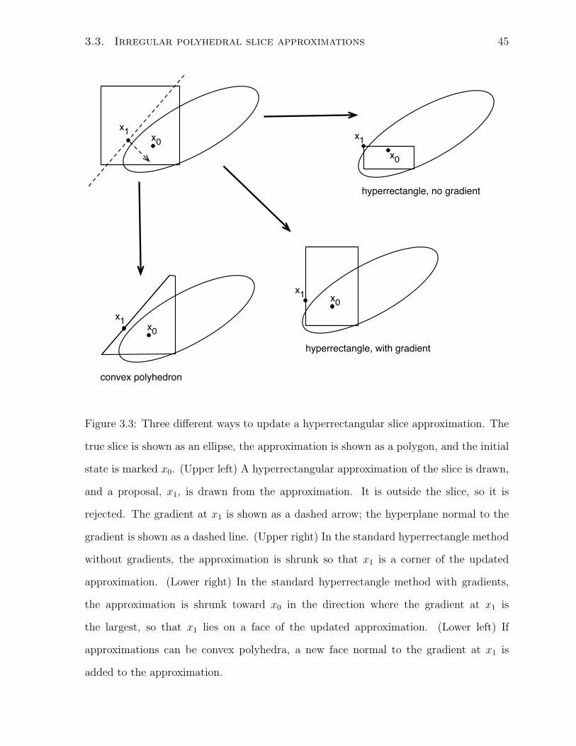
3.3. Irregular polyhedral slice approximations 45
x0x1
x0x1
x0x1
x0
x1
hyperrectangle, no gradient
hyperrectangle, with gradient
convex polyhedron
Figure 3.3: Three different ways to update a hyperrectangular slice approximation. The
true slice is shown as an ellipse, the approximation is shown as a polygon, and the initial
state is marked x0. (Upper left) A hyperrectangular approximation of the slice is drawn,
and a proposal, x1, is drawn from the approximation. It is outside the slice, so it is
rejected. The gradient at x1 is shown as a dashed arrow; the hyperplane normal to the
gradient is shown as a dashed line. (Upper right) In the standard hyperrectangle method
without gradients, the approximation is shrunk so that x1 is a corner of the updated
approximation. (Lower right) In the standard hyperrectangle method with gradients,
the approximation is shrunk toward x0 in the direction where the gradient at x1 is
the largest, so that x1 lies on a face of the updated approximation. (Lower left) If
approximations can be convex polyhedra, a new face normal to the gradient at x1 is
added to the approximation.

46 Chapter 3. Samplers with multivariate steps
motivation for allowing polyhedral slice approximations is that hyperrectangles are not
a tight enough approximation to a slice, this method is infeasible—in high-dimensional
spaces, vanishingly few candidate proposals drawn from a bounding hyperrectangle are
inside the polyhedral slice approximation.
Alternatively, instead of rejection sampling from a bounding hyperrectangle, one could
sample from a bounding ellipsoid with axes not aligned with the coordinate axes. Finding
a minimum-volume ellipsoid containing a convex polyhedron is a convex optimization
problem and can be expressed as a semidefinite program (Boyd and Vandenberghe, 2004,
pp. 169–170). The fastest known way to solve such problems is the barrier method
(Boyd and Vandenberghe, 2004, pp. 261–278), which must estimate O(p2) parameters
each iteration of the Markov chain, and so is prohibitively slow.
A simpler approach is to update the bounding ellipsoid from the previous proposal
instead of finding a new one each time. Given a bounding ellipsoid for proposal k and
a hyperplane normal to the gradient at the rejected proposal, the bounding ellipsoid for
the slice approximation for proposal k + 1 would be the minimum volume ellipsoid that
contains all of the points of the ellipsoid on the same side of the hyperplane as the current
point. This is a well-studied problem; it is at the heart of the ellipsoid method for linear
programming (Grotschel et al., 1993, ch. 3). Unfortunately, the available solutions are not
satisfactory. The expected volume reduction in the ellipsoid is exponentially decreasing
in its dimension. Even though the polyhedron that the ellipsoid approximates shrinks
in volume by a factor independent of dimension on a typical iteration, the bounding
ellipsoid itself shrinks much more slowly. Rejection sampling based on the ellipsoidal
approximation takes unacceptably long if the target distribution has more than a few
dimensions (empirically, around four).
The fundamental problem with this approach is that arbitrarily shaped convex polyhe-
dra are difficult to sample from. Sections 3.4 and 3.5 address this issue by approximating
the slice with a Gaussian distribution instead of a uniform distribution. Since the family

3.4. Covariance matching 47
of Gaussian distributions is conjugate to itself, the proposal distribution conditional on
rejected points remains simple. Yet, it is still possible to derive such a slice approximation
entirely from information obtained in a single MCMC iteration, as with the polyhedral
method described in this section.
3.4 Covariance matching
Sections 3.2 and 3.3 describe methods for taking multivariate steps using uniform pro-
posal distributions. This section takes an alternate approach, using Gaussian proposal
distributions in the crumb framework (Neal, 2003, §5.2). Each sampler iteration in the
crumb framework, a crumb is drawn, and a proposal is drawn from the distribution of
initial states that could have generated that crumb. If the proposal is in the slice, it
is accepted. Otherwise, a second crumb is drawn, a second proposal is drawn from the
distribution of possible initial states conditional on having drawn both crumbs, and so
on until a proposal is accepted.
Crumb distributions may depend on, amongst other things, the log density and gra-
dient at rejected proposals. This section describes one way to choose the crumb dis-
tributions to reduce autocorrelation times on badly scaled distributions with correlated
parameters. The method attempts to match the proposal distribution to the local cur-
vature of the log density. It assumes that while computing the log density at a proposal,
one can compute its gradient with minimal additional cost. This is often a realistic
assumption, since the log density and its gradient are often computed from the same
intermediate values. The human effort required to implement the gradient function is
almost always more relevant.
48 Chapter 3. Samplers with multivariate steps
3.4.1 Adaptive Gaussian crumbs
Let `(·) be the log density of the target distribution, let yslice be the current slice log
density, and let S be the slice through the distribution at that level:
S = {x|`(x) ≥ yslice} (3.5)
Ideally, the proposal distribution would be a uniform distribution over S. To approxi-
mate uniform sampling over S, we draw a sequence of crumbs that produces a Gaussian
proposal distribution with the same covariance matrix as a uniform distribution over S.
Since there are no rejected proposals to adapt on when the first crumb is drawn, the
first crumb has a fixed multivariate Gaussian distribution:
c1 ∼ N(x0,W−11 ) where W1 = σ−2
c I (3.6)
The standard deviation of the initial crumb, σc, is the only tuning parameter for this
method that is modified in normal use; it is reasonable to set it to a guess of the largest
marginal standard deviation of the components of the target distribution divided by the
square root of the distribution’s dimension, as with equation 4.10. Larger values degrade
performance only slightly, so it is better to err on the high side.
The distribution for x0 given c1 is a Gaussian with mean c1 and precision matrix W1,
so we draw a proposal from this distribution:
x1 ∼ N(c1,W−11 ) (3.7)
If `(x1) is at least yslice, then x1 is inside S, so we accept x1 as the next state of the chain.
When a proposal, xk, is not in the slice, we choose a different precision matrix, Wk+1,
for the next crumb, so that the covariance of the next proposal will look more like that
of uniform sampling over S. After sampling k crumbs from Gaussians with mean x0 and
precision matrices (W1, . . . ,Wk), the distribution for the kth proposal (the posterior for
3.4. Covariance matching 49
x0 given the crumbs) is:
xk ∼ N(ck,Λ−1k ) (3.8)
where Λk = W1 + · · ·+Wk (3.9)
and ck = Λ−1k (W1c1 + · · ·+Wkck) (3.10)
The posterior precision is the sum of the precisions of the crumbs; the posterior mean is
the sample mean of the crumbs, weighted by their precisions. If `(xk) is at least yslice, xk
is accepted as the next state. Otherwise, we must choose a covariance for the distribution
of (k + 1)th crumb, draw a new proposal, and repeat until a proposal is accepted.
3.4.2 Adapting the crumb covariance
This section describes a particular method for choosing a precision matrix, Wk+1, for the
(k + 1)th crumb, so that the covariance of the next proposal will approximate that of
uniform sampling over S. Specifically, it attempts to find Wk+1 so that the (k + 1)th
proposal distribution has the same conditional variance as uniform sampling from S in
the direction of the gradient of `(·) at xk. This gradient is a good guess at the direction in
which the proposal distribution is least like S; figure 3.4(a) illustrates this. With a two-
dimensional Gaussian target distribution (with correlation equal to 0.95), I drew a crumb
with σc equal to one and plotted the gradients of the log density at several points drawn
from the resulting proposal distribution. Most of these gradients point in the direction
where the spherically-symmetric proposal variance is least like the slice. Usually, in an
ill-conditioned distribution, gradients at rejected proposals do not point towards a mode,
they point towards the nearest point on the slice. (In a well-conditioned distribution, the
directions to a mode and to the nearest point on the slice will be similar.)
To compute Wk+1, we estimate the second derivative of the target distribution in
the direction of the gradient, assuming the target distribution is approximately locally
Gaussian. Consider the (approximately) parabolic cut through the log-density surface
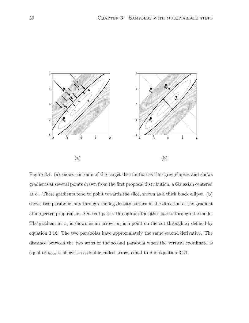
50 Chapter 3. Samplers with multivariate steps
−2
−1
0
1
2
x0●
c1●
−2 −1 0 1 2−2
−1
0
1
2
x0●
c1●
x1●
u1●
−2 −1 0 1 2
(a) (b)
Figure 3.4: (a) shows contours of the target distribution as thin grey ellipses and shows
gradients at several points drawn from the first proposal distribution, a Gaussian centered
at c1. These gradients tend to point towards the slice, shown as a thick black ellipse. (b)
shows two parabolic cuts through the log-density surface in the direction of the gradient
at a rejected proposal, x1. One cut passes through x1; the other passes through the mode.
The gradient at x1 is shown as an arrow. u1 is a point on the cut through x1 defined by
equation 3.16. The two parabolas have approximately the same second derivative. The
distance between the two arms of the second parabola when the vertical coordinate is
equal to yslice is shown as a double-ended arrow, equal to d in equation 3.20.
3.4. Covariance matching 51
passing through x1 in figure 3.4(b). This cut has the equation:
˜1(t) = −1
2κt2 + βt+ γ (3.11)
t is a parameter that is zero at the rejected proposal and increases in the direction of
the gradient; κ, β, and γ are unknown constants we wish to estimate. The coefficient
−12
is arbitrary; this choice makes κ equal to the negative of the second derivative of
the parabola. We already had to compute `(xk) to determine whether xk was in S; we
assume that ∇`(xk) was computed simultaneously. To fix two degrees of freedom of the
parabola, we plug these quantities into equation 3.11 and its derivative with respect to
t:
`(xk) = −1
2κ · 02 + β · 0 + γ = γ (3.12)
‖∇`(xk)‖ = −κ · 0 + β = β (3.13)
There is still one degree of freedom remaining, so we must evaluate `(·) at another point
on the parabola. We choose a point as far away from xk as ck is, hoping that this
distance is within the range where the distribution is approximately Gaussian. Let δ be
this distance:
δ = ‖xk − ck‖ (3.14)
Let g be the normalized gradient at xk:
g =∇`(xk)‖∇`(xk)‖
(3.15)
Then, the point uk is defined to be δ away from xk in the direction g:
uk = xk + δ · g (3.16)
In equation 3.11, uk corresponds to t = δ. We evaluate the log density at uk to fix the
parabolic cut’s third degree of freedom, and plug this into equation 3.11:
`(uk) = −1
2κδ2 + βδ + γ (3.17)
52 Chapter 3. Samplers with multivariate steps
Solving equations 3.12, 3.13, and 3.17 for κ gives:
κ = − 2
δ2
(`(uk)− `(xk)− ‖∇`(xk)‖ · δ
)(3.18)
We can now use κ to approximate the conditional variance in the direction g. If the
Hessian is locally approximately constant, as it is for Gaussians, a cut through the mode
in the direction of ∇`(xk) would have the same second derivative as the cut through xk.
This second parabola, also shown in figure 3.4(b), has the equation:
˜2(t) = −1
2κt2 +M (3.19)
M is the log density at the mode. We set t = 0 at the mode, so there is no linear term.
For now, assume `(·) is unimodal and that M was computed with the conjugate gradient
method (Nocedal and Wright, 2006, ch. 5) or some other similar procedure before starting
the Markov chain. We solve equation 3.19 for the parabola’s diameter d at the level of
the current slice, yslice, shown as a doubled-ended arrow in figure 3.4(b):
d =
√8(M − yslice)
κ(3.20)
Since the distribution of points drawn from an ellipsoidal slice, conditional on their lying
on that particular one-dimensional cut, is uniform with length d, the conditional variance
in the direction of the gradient at xk is:
σ2k+1 =
d2
12=
2
3· M − yslice
κ(3.21)
With this variance, we can construct a crumb precision matrix that will lead to the
desired proposal precision matrix. We want to draw a crumb ck+1 so that the posterior
of x0 given the k crumbs has a variance equal to σ2k+1 in the direction g. Equation 3.9
indicates that the precision of the proposal given these crumbs is:
Λk+1 = Λk +Wk+1 (3.22)
3.4. Covariance matching 53
If we multiply both sides of equation 3.22 by gT on the left and g on the right, the left
side is the conditional precision in the direction g.
gTΛk+1g = gT(Λk +Wk+1
)g (3.23)
We would like to choose Wk+1 so that this conditional precision is σ−2k+1, so we replace
the left hand side of equation 3.23 with that:
σ−2k+1 = gT
(Λk +Wk+1
)g (3.24)
As will be discussed in section 3.4.4, computation will be particularly easy if we choose
Wk+1 to be a scaled copy of Λk with a rank-one update, so we choose Wk+1 to be of the
form:
Wk+1 = θΛk + αggT (3.25)
α and θ are unknown scalars. θ controls how fast the precision as a whole increases. If
we would like the variance in directions other than g to shrink by 9/10, for example,
we choose θ = 1/9. Since θ is constant, there will be exponentially fast convergence
of the proposal covariance in all directions, which allows quick recovery from overly
diffuse initial crumb distributions. For this method, θ is not a critical choice. Setting
θ close to zero causes excessively slow convergence when σc is large relative to the slice
without corresponding benefits when it is small, but a broad range of values larger than
zero give similar performance. I generally set θ to one. Substituting equation 3.25 into
equation 3.24 gives:
σ−2k+1 = gT
(Λk + θΛk + αggT
)g (3.26)
Noting that gTg = 1, we solve for α, obtaining:
α = max{σ−2k+1 − (1 + θ)gTΛkg, 0} (3.27)
α is restricted to be positive to guarantee positive definiteness of the crumb covariance.
(By choosing θ simultaneously, we could perhaps encounter this restriction less frequently,

54 Chapter 3. Samplers with multivariate steps
a possibility I have not explored.) Once we know α, we then compute Wk+1 using
equation 3.25.
The resulting crumb distribution is:
ck+1 ∼ N(x0,W−1k+1) (3.28)
After drawing such a crumb, we draw a proposal according to equations 3.8 to 3.10,
accepting or rejecting depending on whether `(xk+1) ≥ yslice, drawing more crumbs and
adapting until a proposal is accepted.
3.4.3 Estimating the density at the mode
We now modify the covariance matching method to remove the restriction that the target
distribution be unimodal and remove the requirement that we precompute the log density
at the mode. Estimating M each time we update x0 instead of precomputing it allows
M to take on values appropriate to local modes. Since the proposal distribution only
approximates the slice even in the best of circumstances, it is not essential that the
estimate of M be particularly good.
To estimate M , we initialize M to yslice before drawing the first crumb. Then, every
time we fit the parabola described by equation 3.11, we update M to be the maximum
of the current value of M and the estimated peak of the parabola. As more crumbs
are drawn, M becomes a better estimate of the local maximum. We could also use the
values of the log density at rejected proposals and at the {uk} to bound M , but if the
log density is locally concave, the log densities at the peaks of the parabola will always
be larger than these values.
3.4.4 Efficient computation of the crumb covariance
This section describes a method for using Cholesky factors of precision matrices to make
implementation of the covariance matching method of section 3.4.2 efficient. If imple-
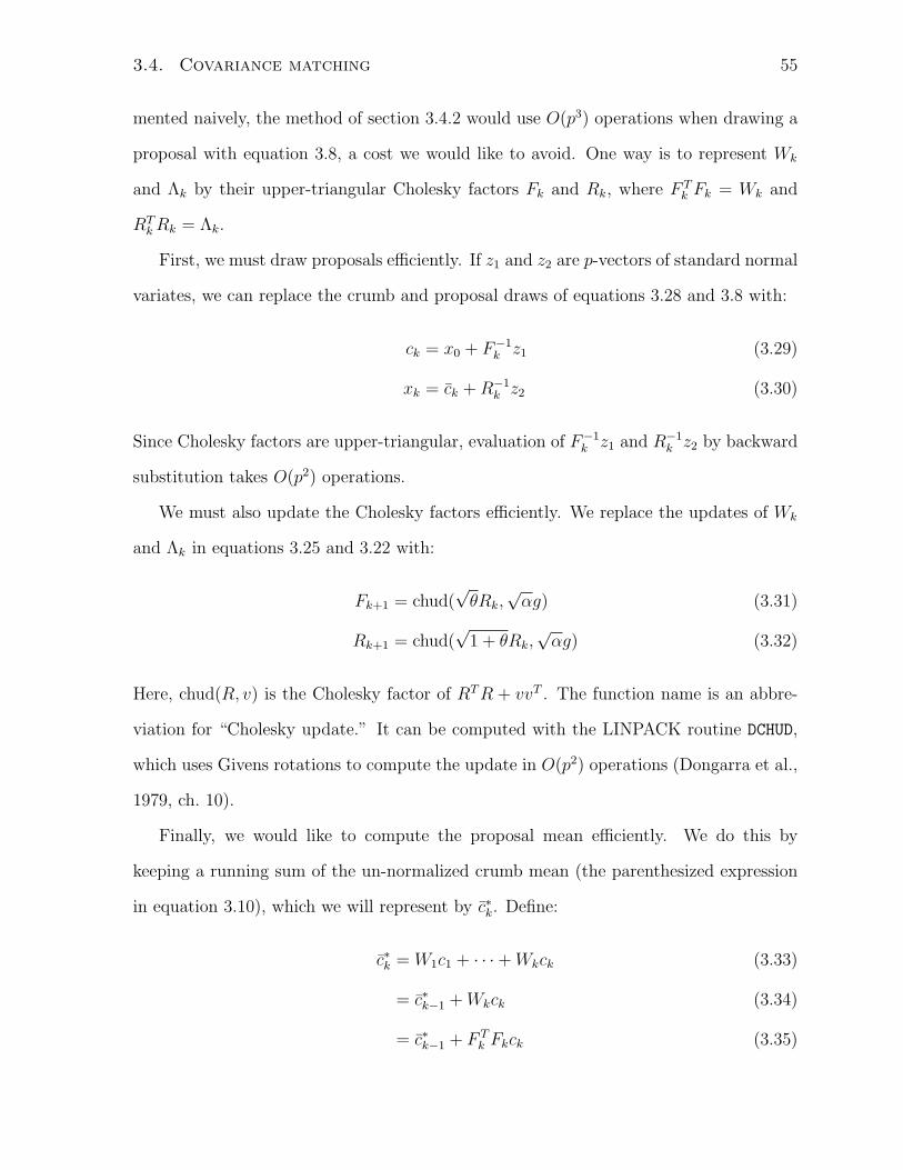
3.4. Covariance matching 55
mented naively, the method of section 3.4.2 would use O(p3) operations when drawing a
proposal with equation 3.8, a cost we would like to avoid. One way is to represent Wk
and Λk by their upper-triangular Cholesky factors Fk and Rk, where F Tk Fk = Wk and
RTkRk = Λk.
First, we must draw proposals efficiently. If z1 and z2 are p-vectors of standard normal
variates, we can replace the crumb and proposal draws of equations 3.28 and 3.8 with:
ck = x0 + F−1k z1 (3.29)
xk = ck +R−1k z2 (3.30)
Since Cholesky factors are upper-triangular, evaluation of F−1k z1 and R−1
k z2 by backward
substitution takes O(p2) operations.
We must also update the Cholesky factors efficiently. We replace the updates of Wk
and Λk in equations 3.25 and 3.22 with:
Fk+1 = chud(√θRk,
√αg) (3.31)
Rk+1 = chud(√
1 + θRk,√αg) (3.32)
Here, chud(R, v) is the Cholesky factor of RTR + vvT . The function name is an abbre-
viation for “Cholesky update.” It can be computed with the LINPACK routine DCHUD,
which uses Givens rotations to compute the update in O(p2) operations (Dongarra et al.,
1979, ch. 10).
Finally, we would like to compute the proposal mean efficiently. We do this by
keeping a running sum of the un-normalized crumb mean (the parenthesized expression
in equation 3.10), which we will represent by c∗k. Define:
c∗k = W1c1 + · · ·+Wkck (3.33)
= c∗k−1 +Wkck (3.34)
= c∗k−1 + F Tk Fkck (3.35)

56 Chapter 3. Samplers with multivariate steps
Then, using forward and backward substitution, we can compute the normalized crumb
mean, ck, as:
ck = R−1k R−Tk c∗k (3.36)
This way, we can compute ck in O(p2) operations and do not need to save all the crumbs
and crumb covariances.
With these changes, the resulting algorithm is numerically stable even with ill con-
ditioned target distributions. Each crumb and proposal draw takes O(p2) operations.
Figure 3.5 shows pseudocode for a single iteration.
3.5 Shrinking rank proposals
This section presents a second MCMC method in the crumb framework, shrinking rank. It
is simpler than covariance matching, but retains its desirable properties. Like covariance
matching, shrinking rank draws a sequence of Gaussian crumbs with mean equal to
the current state and variance chosen adaptively based on information from rejected
proposals. Instead of attempting to match the curvature of the log density along the
gradient, however, it sets the crumb variance in that direction to zero, causing subsequent
proposals to have a variance of zero in that direction as well. This technique aims to
cause proposal variances to be nonzero only in the longest direction of the slice, which is
usually the slowest mixing one.
Each iteration begins by drawing a slice level as discussed in section 3.1:
yslice = `(x0)− E where E ∼ Exponential(1) (3.37)
When the first crumb, c1, is drawn, there are no previous proposals providing information
to adapt on, so it is drawn from a spherical Gaussian distribution with marginal standard
deviation σc, where σc is a tuning parameter. The distribution for the first proposal, x1,
is also a spherical Gaussian with standard deviation σc but centered at c1 instead of x0.

3.5. Shrinking rank proposals 57
One step in the covariance matching method
initialize `, x0 ∈ Rp, σc, and θ.
M ← `(x0)
yslice ←M − draw from Exponential(1)
R← σ−1c I
F ← σ−1c I
c∗ ← 0
repeat until a proposal is accepted:
z ← draw fromNp(0, I)
c← x0 + F−1z
c∗ ← c∗ + F TFc
c← R−1R−T c∗
z ← draw fromNp(0, I)
x← c+R−1z
y ← `(x)
if y ≥ yslice:
accept proposal x.
end (if)
G← ∇`(x)
g ← G/‖G‖δ ← ‖x− c‖u← x+ δg
`u ← `(u)
κ← −2δ−2 (`u − y − δ‖G‖)`x,u ← 1
2‖G‖2κ
+ y
M ← max {M, `x,u}σ2 ← 2
3M−yslice
κ
α← max{
0, σ−2 − (1 + θ)gTRTRg}
F ← chud(√
θR,√αg)
R← chud(√
1 + θR,√αg)
end (repeat)
Figure 3.5: A single iteration of the adaptive algorithm of section 3.4. The variables are
mostly the same as in the text. The k subscript is dropped since there is no need to keep
copies of the values from any but the most recent iteration. The variable `x,u indicates
the peak of the parabolic cut through x and u.

58 Chapter 3. Samplers with multivariate steps
x0●
c1●
x1●
x0●x1●
c1●
c2●x2●
(a) (b)
Figure 3.6: (a) The grey lines represent the contours of a two-dimensional distribution;
the solid ellipse represents the boundary of the slice. The first crumb, c1, is drawn from
a spherical Gaussian represented by a dotted circle; a proposal, x1, is drawn from a
spherical Gaussian centered at c1, represented by a dashed circle. x1 is rejected because
it is outside the solid ellipse. (b) A second crumb, c2, is drawn from a reduced-rank
subspace, represented by a dashed line. A second proposal, x2, is drawn from the same
subspace. Since x2 is inside the solid ellipse, it is accepted.
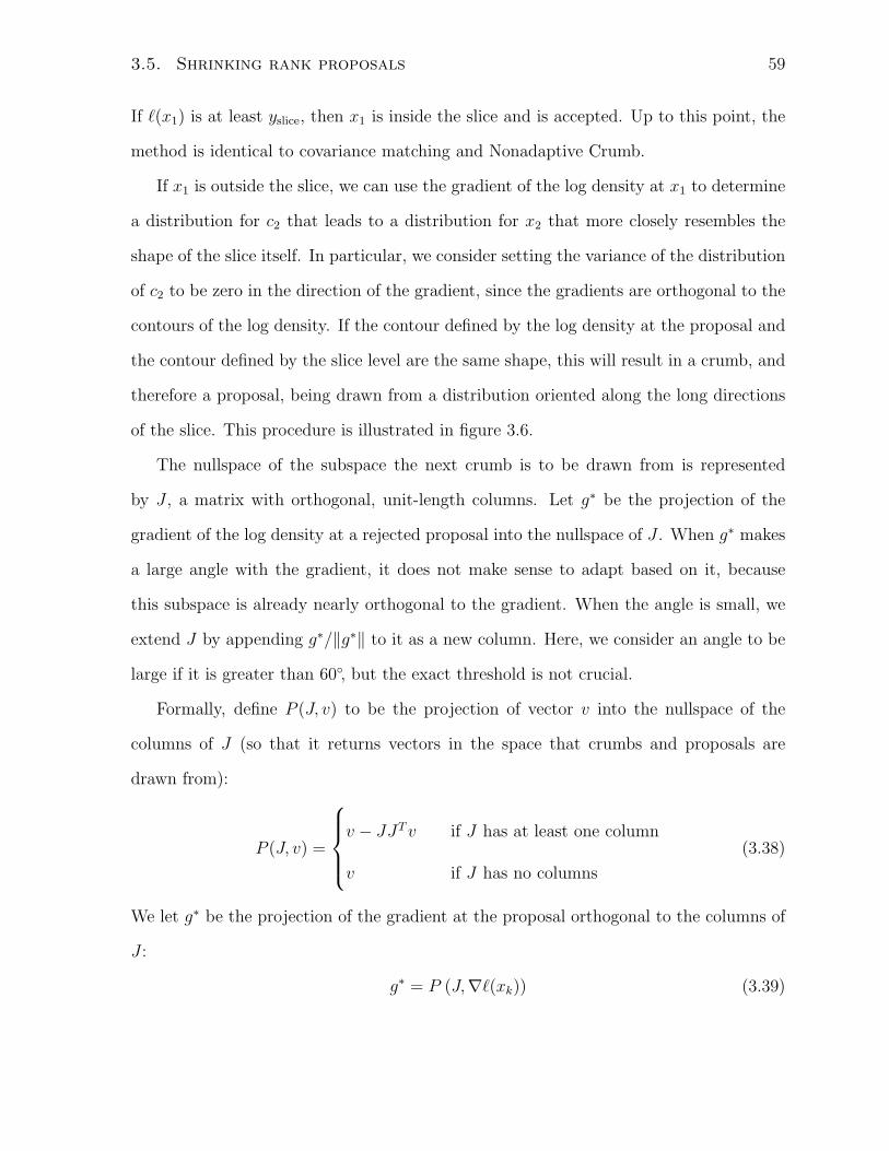
3.5. Shrinking rank proposals 59
If `(x1) is at least yslice, then x1 is inside the slice and is accepted. Up to this point, the
method is identical to covariance matching and Nonadaptive Crumb.
If x1 is outside the slice, we can use the gradient of the log density at x1 to determine
a distribution for c2 that leads to a distribution for x2 that more closely resembles the
shape of the slice itself. In particular, we consider setting the variance of the distribution
of c2 to be zero in the direction of the gradient, since the gradients are orthogonal to the
contours of the log density. If the contour defined by the log density at the proposal and
the contour defined by the slice level are the same shape, this will result in a crumb, and
therefore a proposal, being drawn from a distribution oriented along the long directions
of the slice. This procedure is illustrated in figure 3.6.
The nullspace of the subspace the next crumb is to be drawn from is represented
by J , a matrix with orthogonal, unit-length columns. Let g∗ be the projection of the
gradient of the log density at a rejected proposal into the nullspace of J . When g∗ makes
a large angle with the gradient, it does not make sense to adapt based on it, because
this subspace is already nearly orthogonal to the gradient. When the angle is small, we
extend J by appending g∗/‖g∗‖ to it as a new column. Here, we consider an angle to be
large if it is greater than 60◦, but the exact threshold is not crucial.
Formally, define P (J, v) to be the projection of vector v into the nullspace of the
columns of J (so that it returns vectors in the space that crumbs and proposals are
drawn from):
P (J, v) =
v − JJTv if J has at least one column
v if J has no columns
(3.38)
We let g∗ be the projection of the gradient at the proposal orthogonal to the columns of
J :
g∗ = P (J,∇`(xk)) (3.39)
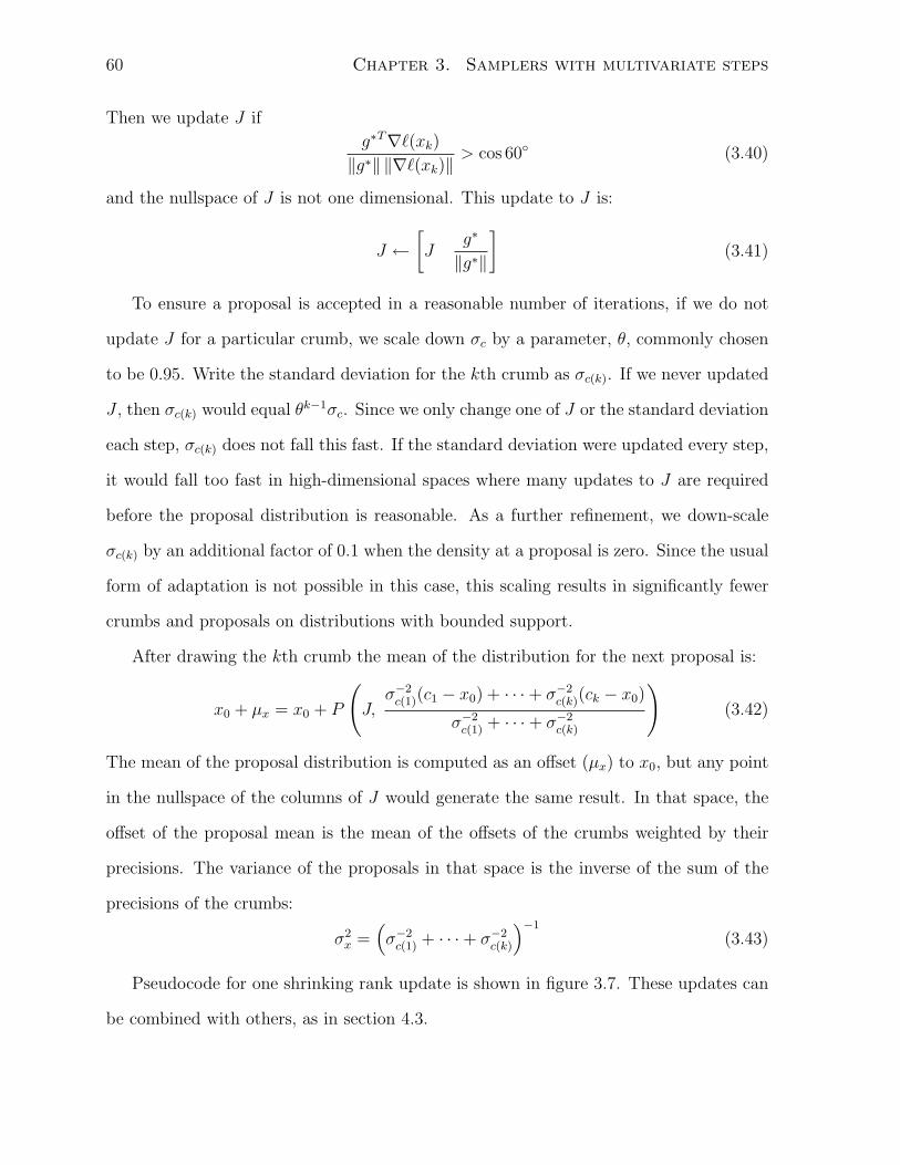
60 Chapter 3. Samplers with multivariate steps
Then we update J if
g∗T∇`(xk)‖g∗‖ ‖∇`(xk)‖
> cos 60◦ (3.40)
and the nullspace of J is not one dimensional. This update to J is:
J ←[J
g∗
‖g∗‖
](3.41)
To ensure a proposal is accepted in a reasonable number of iterations, if we do not
update J for a particular crumb, we scale down σc by a parameter, θ, commonly chosen
to be 0.95. Write the standard deviation for the kth crumb as σc(k). If we never updated
J , then σc(k) would equal θk−1σc. Since we only change one of J or the standard deviation
each step, σc(k) does not fall this fast. If the standard deviation were updated every step,
it would fall too fast in high-dimensional spaces where many updates to J are required
before the proposal distribution is reasonable. As a further refinement, we down-scale
σc(k) by an additional factor of 0.1 when the density at a proposal is zero. Since the usual
form of adaptation is not possible in this case, this scaling results in significantly fewer
crumbs and proposals on distributions with bounded support.
After drawing the kth crumb the mean of the distribution for the next proposal is:
x0 + µx = x0 + P
(J,
σ−2c(1)(c1 − x0) + · · ·+ σ−2
c(k)(ck − x0)
σ−2c(1) + · · ·+ σ−2
c(k)
)(3.42)
The mean of the proposal distribution is computed as an offset (µx) to x0, but any point
in the nullspace of the columns of J would generate the same result. In that space, the
offset of the proposal mean is the mean of the offsets of the crumbs weighted by their
precisions. The variance of the proposals in that space is the inverse of the sum of the
precisions of the crumbs:
σ2x =
(σ−2c(1) + · · ·+ σ−2
c(k)
)−1
(3.43)
Pseudocode for one shrinking rank update is shown in figure 3.7. These updates can
be combined with others, as in section 4.3.
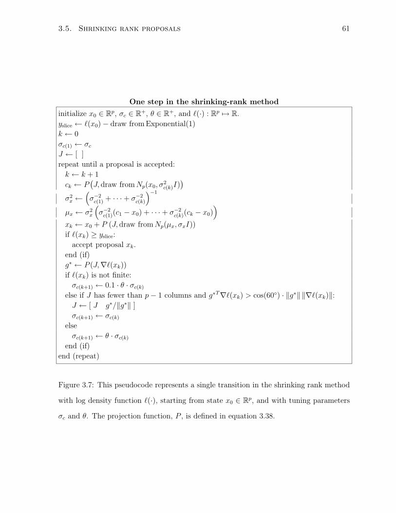
3.5. Shrinking rank proposals 61
One step in the shrinking-rank method
initialize x0 ∈ Rp, σc ∈ R+, θ ∈ R+, and `(·) : Rp 7→ R.
yslice ← `(x0)− draw from Exponential(1)
k ← 0
σc(1) ← σcJ ← [ ]
repeat until a proposal is accepted:
k ← k + 1
ck ← P(J, draw fromNp(x0, σ
2c(k)I)
)σ2x ←
(σ−2c(1) + · · ·+ σ−2
c(k)
)−1
µx ← σ2x
(σ−2c(1)(c1 − x0) + · · ·+ σ−2
c(k)(ck − x0))
xk ← x0 + P (J, draw fromNp(µx, σxI))
if `(xk) ≥ yslice:
accept proposal xk.
end (if)
g∗ ← P (J,∇`(xk))if `(xk) is not finite:
σc(k+1) ← 0.1 · θ · σc(k)
else if J has fewer than p− 1 columns and g∗T∇`(xk) > cos(60◦) · ‖g∗‖ ‖∇`(xk)‖:J ← [ J g∗/‖g∗‖ ]
σc(k+1) ← σc(k)
else
σc(k+1) ← θ · σc(k)
end (if)
end (repeat)
Figure 3.7: This pseudocode represents a single transition in the shrinking rank method
with log density function `(·), starting from state x0 ∈ Rp, and with tuning parameters
σc and θ. The projection function, P , is defined in equation 3.38.
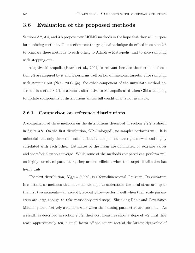
62 Chapter 3. Samplers with multivariate steps
3.6 Evaluation of the proposed methods
Sections 3.2, 3.4, and 3.5 propose new MCMC methods in the hope that they will outper-
form existing methods. This section uses the graphical technique described in section 2.3
to compare these methods to each other, to Adaptive Metropolis, and to slice sampling
with stepping out.
Adaptive Metropolis (Haario et al., 2001) is relevant because the methods of sec-
tion 3.2 are inspired by it and it performs well on low dimensional targets. Slice sampling
with stepping out (Neal, 2003, §4), the other component of the univariate method de-
scribed in section 3.2.1, is a robust alternative to Metropolis used when Gibbs sampling
to update components of distributions whose full conditional is not available.
3.6.1 Comparison on reference distributions
A comparison of these methods on the distributions described in section 2.2.2 is shown
in figure 3.8. On the first distribution, GP (unlogged), no sampler performs well. It is
unimodal and only three-dimensional, but its components are right-skewed and highly
correlated with each other. Estimates of the mean are dominated by extreme values
and therefore slow to converge. While some of the methods compared can perform well
on highly correlated parameters, they are less efficient when the target distribution has
heavy tails.
The next distribution, N4(ρ = 0.999), is a four-dimensional Gaussian. Its curvature
is constant, so methods that make an attempt to understand the local structure up to
the first two moments—all except Step-out Slice—perform well when their scale param-
eters are large enough to take reasonably-sized steps. Shrinking Rank and Covariance
Matching are effectively a random walk when their tuning parameters are too small. As
a result, as described in section 2.3.2, their cost measures show a slope of −2 until they
reach approximately ten, a small factor off the square root of the largest eigenvalue of
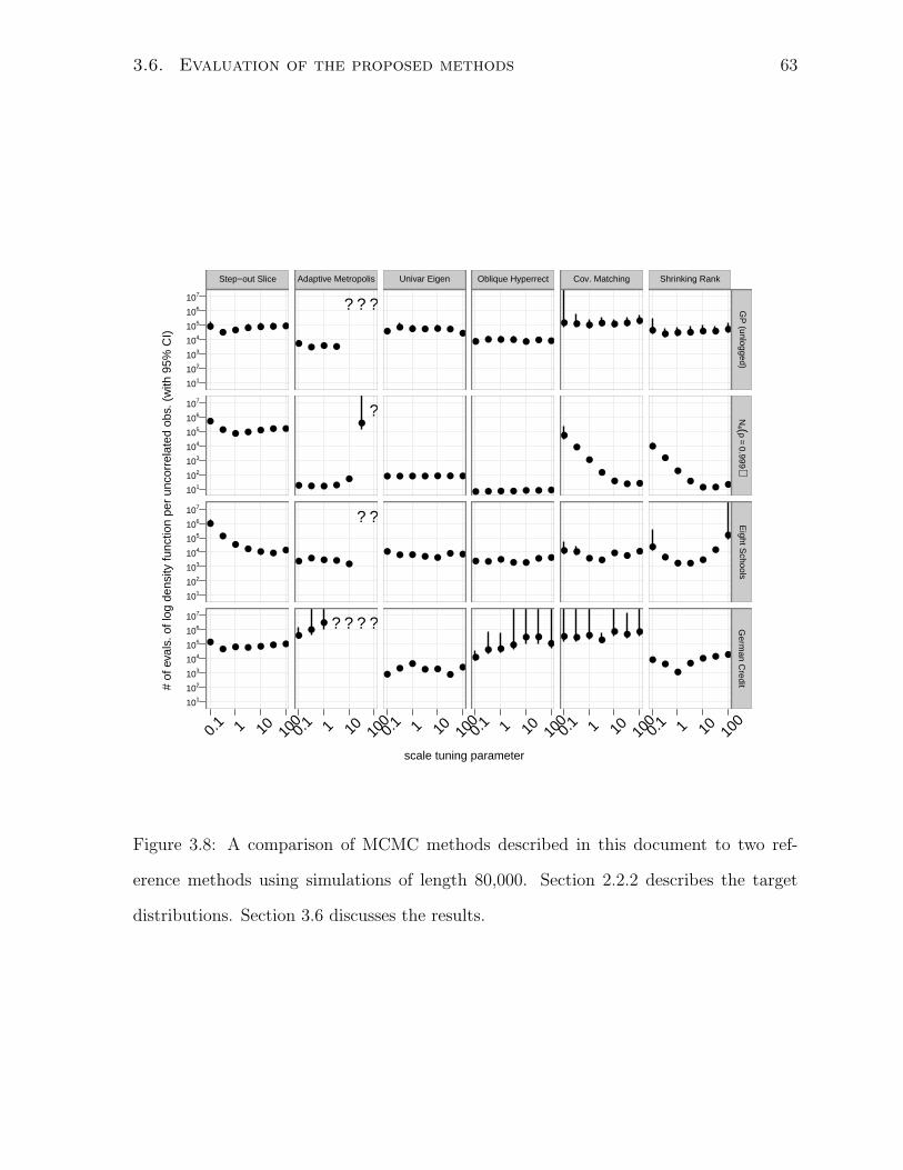
3.6. Evaluation of the proposed methods 63
scale tuning parameter
# of
eva
ls. o
f log
den
sity
func
tion
per
unco
rrel
ated
obs
. (w
ith 9
5% C
I)
101
102
103
104
105
106
107
101
102
103
104
105
106
107
101
102
103
104
105
106
107
101
102
103
104
105
106
107
Step−out Slice
●● ● ● ● ● ●
●●●●●●●
●●●●●
●
●
●●●●●●●
0.1 1 10 10
0
Adaptive Metropolis
● ● ● ●
? ? ?
●
●●●●●
?
●●●●●
??
●●
●????
0.1 1 10 10
0
Univar Eigen
● ● ● ● ● ● ●
● ● ● ● ● ● ●
● ● ● ● ● ● ●
●●
●● ●
●●
0.1 1 10 10
0
Oblique Hyperrect
● ● ● ● ● ● ●
● ● ● ● ● ● ●
● ● ● ● ● ● ●
●● ● ●
● ●●
0.1 1 10 10
0
Cov. Matching
● ● ● ● ● ● ●
●
●
●
●● ● ●
● ●● ●
● ●●
● ● ●●
● ● ●
0.1 1 10 10
0
Shrinking Rank
● ● ● ● ● ● ●
●
●
●●
● ● ●
●●
● ● ●●
●
●●
●●
● ● ●
0.1 1 10 10
0
GP
(unlogged)N
4 (ρ=
0.999)E
ight Schools
Germ
an Credit
Figure 3.8: A comparison of MCMC methods described in this document to two ref-
erence methods using simulations of length 80,000. Section 2.2.2 describes the target
distributions. Section 3.6 discusses the results.

64 Chapter 3. Samplers with multivariate steps
the covariance matrix.
The third distribution, Eight Schools, is well conditioned and is not substantially
skewed. As a result, every sampler tested performs similarly on it when their tuning
parameters are in a reasonable range. As before, the slice samplers that do not do
global adaptation (Shrinking Rank, Covariance Matching, and Step-out Slice) perform
well for sufficiently large tuning parameters, and Adaptive Metropolis performs well for
sufficiently small ones. Globally adaptive slice samplers (Oblique Hyperrect and Univar
Eigen) perform well for all tuning parameters tested, assuming they are run long enough
to learn the covariance matrix.
The fourth distribution, German Credit, is 25-dimensional, so its covariance has 325
degrees of freedom. Shrinking Rank, Oblique Hyperrect, and Univar Eigen all perform
reasonably well on it, but the adaptation required makes their performance more idiosyn-
cratic on German Credit than on other distributions.
3.6.2 Comparison on a latent AR process
This section extends the comparison of section 3.6 by comparing the same six sam-
plers on a family of latent jump-autoregressive processes. In this model, one observes
a sequence of N Bernoulli random variables {Yi}Ni=1 such that Yi = 1 with probability
1/(1 + exp(−Xi)). The {Xi} are themselves generated by a mean-zero autoregressive
process with an autocorrelation of α, a probability ρ of a jump to an uncorrelated state,
and a variance σ2. The parameters σ2, α, and ρ are transformed and given Student-t
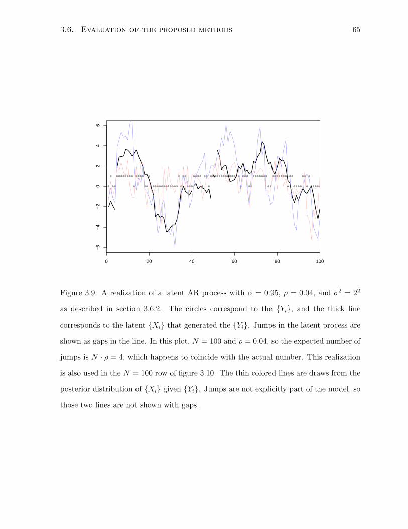
3.6. Evaluation of the proposed methods 65
0 20 40 60 80 100
−6
−4
−2
02
46
Figure 3.9: A realization of a latent AR process with α = 0.95, ρ = 0.04, and σ2 = 22
as described in section 3.6.2. The circles correspond to the {Yi}, and the thick line
corresponds to the latent {Xi} that generated the {Yi}. Jumps in the latent process are
shown as gaps in the line. In this plot, N = 100 and ρ = 0.04, so the expected number of
jumps is N · ρ = 4, which happens to coincide with the actual number. This realization
is also used in the N = 100 row of figure 3.10. The thin colored lines are draws from the
posterior distribution of {Xi} given {Yi}. Jumps are not explicitly part of the model, so
those two lines are not shown with gaps.
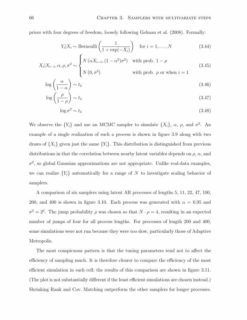
66 Chapter 3. Samplers with multivariate steps
priors with four degrees of freedom, loosely following Gelman et al. (2008). Formally:
Yi|Xi ∼ Bernoulli
(1
1 + exp(−Xi)
)for i = 1, . . . , N (3.44)
Xi|Xi−1, α, ρ, σ2 ∼
N (αXi−1, (1− α2)σ2) with prob. 1− ρ
N (0, σ2) with prob. ρ or when i = 1
(3.45)
log
(α
1− α
)∼ t4 (3.46)
log
(ρ
1− ρ
)∼ t4 (3.47)
log σ2 ∼ t4 (3.48)
We observe the {Yi} and use an MCMC sampler to simulate {Xi}, α, ρ, and σ2. An
example of a single realization of such a process is shown in figure 3.9 along with two
draws of {Xi} given just the same {Yi}. This distribution is distinguished from previous
distributions in that the correlation between nearby latent variables depends on ρ, α, and
σ2, so global Gaussian approximations are not appropriate. Unlike real-data examples,
we can realize {Yi} automatically for a range of N to investigate scaling behavior of
samplers.
A comparison of six samplers using latent AR processes of lengths 5, 11, 22, 47, 100,
200, and 400 is shown in figure 3.10. Each process was generated with α = 0.95 and
σ2 = 22. The jump probability ρ was chosen so that N · ρ = 4, resulting in an expected
number of jumps of four for all process lengths. For processes of length 200 and 400,
some simulations were not run because they were too slow, particularly those of Adaptive
Metropolis.
The most conspicuous pattern is that the tuning parameters tend not to affect the
efficiency of sampling much. It is therefore clearer to compare the efficiency of the most
efficient simulation in each cell; the results of this comparison are shown in figure 3.11.
(The plot is not substantially different if the least efficient simulations are chosen instead.)
Shrinking Rank and Cov. Matching outperform the other samplers for longer processes.
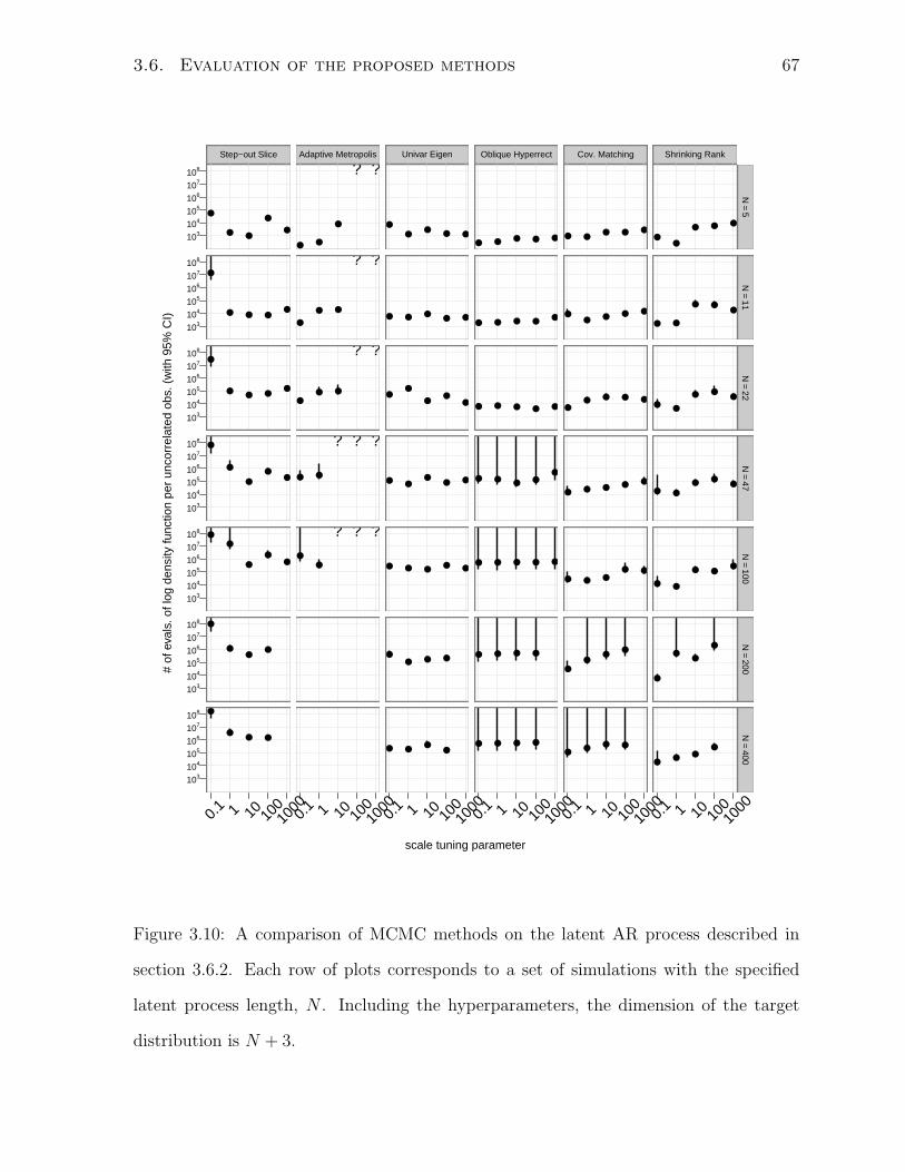
3.6. Evaluation of the proposed methods 67
scale tuning parameter
# of
eva
ls. o
f log
den
sity
func
tion
per
unco
rrel
ated
obs
. (w
ith 9
5% C
I)
103104105106107108
103104105106107108
103104105106107108
103104105106107108
103104105106107108
103104105106107108
103104105106107108
Step−out Slice
●
● ●
●
●
●
● ● ●●
●
● ● ●●
●
●
●●
●
●●
●●
●
●
●
●●
●
●
● ●
0.1 1 10 10
010
00
Adaptive Metropolis
● ●
●
? ?
●
● ●
? ?
●● ●
? ?
● ●
? ? ?
●●
? ? ?
0.1 1 10 10
010
00
Univar Eigen
●●
● ● ●
● ● ●● ●
●●
●●
●
● ●●
● ●
● ● ● ● ●
●● ● ●
● ●●
●
0.1 1 10 10
010
00
Oblique Hyperrect
● ● ● ● ●
● ● ● ● ●
● ● ● ● ●
● ● ● ●●
● ● ● ● ●
● ● ● ●
● ● ● ●
0.1 1 10 10
010
00
Cov. Matching
● ●● ● ●
●● ● ● ●
●● ● ● ●
● ● ● ● ●
● ● ●● ●
●●
●●
● ● ● ●
0.1 1 10 10
010
00
Shrinking Rank
●●
● ● ●
● ●
● ●●
● ●
● ●●
● ●● ●
●
● ●
● ●●
●
●●
●
●● ●
●
0.1 1 10 10
010
00
N=
5N
=11
N=
22N
=47
N=
100N
=200
N=
400
Figure 3.10: A comparison of MCMC methods on the latent AR process described in
section 3.6.2. Each row of plots corresponds to a set of simulations with the specified
latent process length, N . Including the hyperparameters, the dimension of the target
distribution is N + 3.
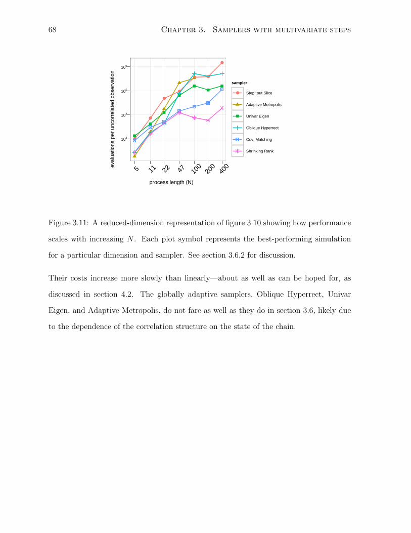
68 Chapter 3. Samplers with multivariate steps
process length (N)
eval
uatio
ns p
er u
ncor
rela
ted
obse
rvat
ion
103
104
105
106
●
●
●
●
● ●
●
5 11 22 47 100
200
400
sampler
● Step−out Slice
Adaptive Metropolis
Univar Eigen
Oblique Hyperrect
Cov. Matching
Shrinking Rank
Figure 3.11: A reduced-dimension representation of figure 3.10 showing how performance
scales with increasing N . Each plot symbol represents the best-performing simulation
for a particular dimension and sampler. See section 3.6.2 for discussion.
Their costs increase more slowly than linearly—about as well as can be hoped for, as
discussed in section 4.2. The globally adaptive samplers, Oblique Hyperrect, Univar
Eigen, and Adaptive Metropolis, do not fare as well as they do in section 3.6, likely due
to the dependence of the correlation structure on the state of the chain.
Chapter 4
Scaling and radial steps
If a random variable X has a log density function `(·), then `(X) is a scalar random
variable. For many p-dimensional probability distributions, this random variable has
a standard deviation proportional to√p (Roberts and Rosenthal, 2002; Neal, 2003,
pp. 758–760). Multivariate slice sampler updates change the log density by at most
O(1) each iteration using the exponential draws of section 3.1, so they take at least O(p)
iterations to reach an independent state. (The updates of random-walk Metropolis work
differently but scale similarly.) This chapter explores this scaling behavior and proposes
methods to improve it. First, it describes the scaling of simple and idealized slice sam-
plers to establish a baseline and to identify proper tuning parameters. Then, it extends
the comparison to more realistic distributions and shows how the scaling of practical
methods can be improved with radial steps toward or away from a local mode.
4.1 Optimal tuning of Gaussian crumbs
4.1.1 Scaling on slices of known radius
A representative example of a slice sampler that takes multivariate steps is slice sampling
with nonadaptive Gaussian crumbs (Neal, 2003, §5.2), on which the covariance matching
69
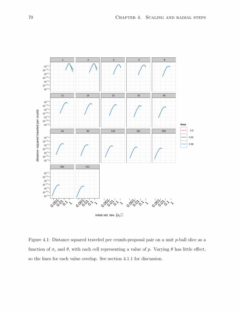
70 Chapter 4. Scaling and radial steps
initial std. dev. (σc)
dist
ance
−sq
uare
d tr
avel
ed p
er c
rum
b
10−4
10−3.5
10−3
10−2.5
10−2
10−1.5
10−1
10−4
10−3.5
10−3
10−2.5
10−2
10−1.5
10−1
10−4
10−3.5
10−3
10−2.5
10−2
10−1.5
10−1
10−4
10−3.5
10−3
10−2.5
10−2
10−1.5
10−1
1
11
64
362
0.00
10.
01 0.1 1
2
16
90
512
0.00
10.
01 0.1 1
4
22
128
0.00
10.
01 0.1 1
5
32
181
0.00
10.
01 0.1 1
8
45
256
0.00
10.
01 0.1 1
theta
0.9
0.95
0.98
Figure 4.1: Distance squared traveled per crumb-proposal pair on a unit p-ball slice as a
function of σc and θ, with each cell representing a value of p. Varying θ has little effect,
so the lines for each value overlap. See section 4.1.1 for discussion.
4.1. Optimal tuning of Gaussian crumbs 71
method of section 3.4 and the shrinking rank method of section 3.5 are based. The
method draws crumbs from a sequence of Gaussians centered at the current state, drawing
proposals from the posterior distribution for the current state given the crumbs. While a
method in the crumb framework may adapt the crumb distribution based on log densities
at rejected proposals (amongst other possibilities) as in sections 3.4 and 3.5, this section
focuses on the non-adaptive case where the crumb distribution depends only on how
many crumbs have been drawn.
With non-adaptive Gaussian crumbs, there are two free parameters: the standard
deviation of the distribution of the first crumb (σc) and the rate with which the standard
deviation of successive crumbs falls (θ). This section describes an experiment intended
to identify reasonable values for these parameters when the shape and scale of the slice
is known. Suppose the slice from which we want to draw an update is a p-ball of known
radius R, but we do not know its location. Given an initial state x0, we would like use the
Gaussian crumb method to draw a new point from the slice. To do this, for k = 1, 2, . . .,
we draw crumb k:
ck ∼ Np
(x0, σ
2(k)I)
(4.1)
and then draw proposal k from the posterior distribution of x0 given the sequence of
crumbs, {c1, . . . , ck}:
xk ∼ Np
(ck,Λ
−1k
)(4.2)
where: Λk =(σ−2
(1) + · · ·+ σ−2(k)
)I (4.3)
and: ck = Λ−1k
(σ−2
(1)c1 + · · ·+ σ−2(k)ck
)(4.4)
If x0 is near the edge of the slice, a larger number of proposals will be rejected before one
is accepted than if x0 were in the interior of the slice. So, the optimal crumb standard
deviation depends on x0. Since x0 is unknown (from the perspective of proposals), we
start with a large σ(1) and decrease it quickly so that the elements of the proposal variance,
Λ−1k , decrease exponentially rather than linearly in terms of k as would happen if the
72 Chapter 4. Scaling and radial steps
crumb standard deviation were constant.
Take the standard deviation of the kth crumb to be of the form:
σ(k) = σcθk−1R (4.5)
Both σc and θ can depend arbitrarily on p. For this experiment, I fix the slice radius, R,
to one. The method is scale invariant, so by making the standard deviation proportional
to the slice radius, the results generalize to any slice known to be a p-ball.
When p is larger than two or three, each individual step is small relative to the scale
of the distribution because most of the mass of a p-ball is very close to its surface. As a
result, the sequence of states is approximately a random walk. In r steps, a random walk
travels O(√r) distance, so the correlation between pairs of states of a random walk is
minimized by maximizing the expected squared distance of an individual step (Pasarica
and Gelman, 2010, §1.2). To determine the σc and θ that lead to the highest average
squared distance traveled per log density evaluation (of which there is one per crumb-
proposal pair), I simulated 5,000 MCMC iterations for a range of θ, σc, and p. The
results of this experiment are plotted in figure 4.1.
In this experiment and in one that explored θ ranging from 0.01 to 10, the performance
does not appear to depend much on θ, as long as it is less than one. Choosing θ to be
exactly one leads to qualitatively worse performance, though 0.99 does not. Therefore, I
am comfortable fixing θ to be 0.95 for the experiments in this section.
Next, to find the σc with the best squared distance traveled per crumb as a function
of p with R fixed at one, I fit the following linear model to the optimal σc for each p:
log σc = β0 + β1 log p+ ε (4.6)
For dimensions greater than two, the fit is quite good. A 95% confidence interval for β1,
the exponent on p, is (−1.01,−0.94) with a regression R-squared of 0.997. To simplify,
I round β1 to −1, yielding the following expression for the optimal σc:
σc =2.6
p(4.7)
4.1. Optimal tuning of Gaussian crumbs 73
Using equation 4.7, we choose the standard deviation of the kth crumb to be:
σ(k) = 2.6 · 0.95k−1 · Rp
(4.8)
4.1.2 Scaling on slices of χp radius
The previous section established optimal tuning parameters for slice sampling with Gaus-
sian crumbs when we know that the slice is a p-ball with radius R. This may not be
practical. But, it is not unreasonable to assume we know, through some sort of adapta-
tion, the shape of the slice. If the slices are ellipsoids known up to a unknown scale factor
and an unknown translation, the results of section 4.1.1 apply by affine transform of the
crumb distribution. However, while we may be willing to approximate the slice with an
ellipsoid, and we can estimate the shape of such an ellipsoid using the sample covariance
(or a variant that takes into account local structure), we do not know the scale of the
slice. That is, even if we know everything there is to know about the target distribution,
since the log density may not be normalized, we cannot, in general, determine the scale
factor, R, from just the slice level and shape. This section attempts to find an optimal
σc given p but not R.
A standard p-dimensional Gaussian has log density:
`(x) = −‖x‖2
2+ C (4.9)
C is an unknown constant (equal to −p2
log 2π if the distribution is normalized). Since
‖x‖2 has a χ2p distribution, slices from this distribution are of the form ‖x‖2 < R2 for
some value of R, with the squared slice radii, R2, having a χ2p distribution. So, to find
an optimal σc and θ, we can simulate R2 from a χ2p distribution instead of setting R to
one to see which σc and θ lead to the best general performance.
Using this method of generating R, I repeated the experiment of section 4.1.1. The
results are shown in figure 4.2. I repeated the analysis of section 4.1.1 to obtain a
curve for the the optimal standard deviation for the kth crumb. The resulting fit is
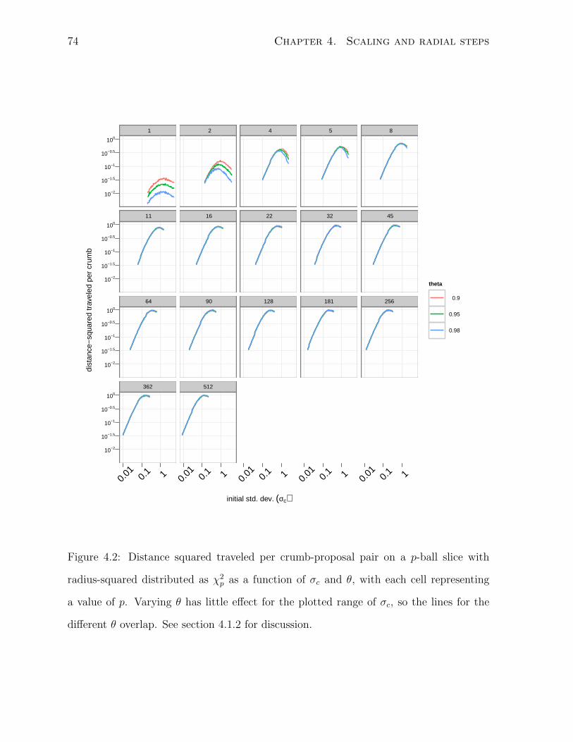
74 Chapter 4. Scaling and radial steps
initial std. dev. (σc)
dist
ance
−sq
uare
d tr
avel
ed p
er c
rum
b
10−2
10−1.5
10−1
10−0.5
100
10−2
10−1.5
10−1
10−0.5
100
10−2
10−1.5
10−1
10−0.5
100
10−2
10−1.5
10−1
10−0.5
100
1
11
64
362
0.01 0.
1 1
2
16
90
512
0.01 0.
1 1
4
22
128
0.01 0.
1 1
5
32
181
0.01 0.
1 1
8
45
256
0.01 0.
1 1
theta
0.9
0.95
0.98
Figure 4.2: Distance squared traveled per crumb-proposal pair on a p-ball slice with
radius-squared distributed as χ2p as a function of σc and θ, with each cell representing
a value of p. Varying θ has little effect for the plotted range of σc, so the lines for the
different θ overlap. See section 4.1.2 for discussion.
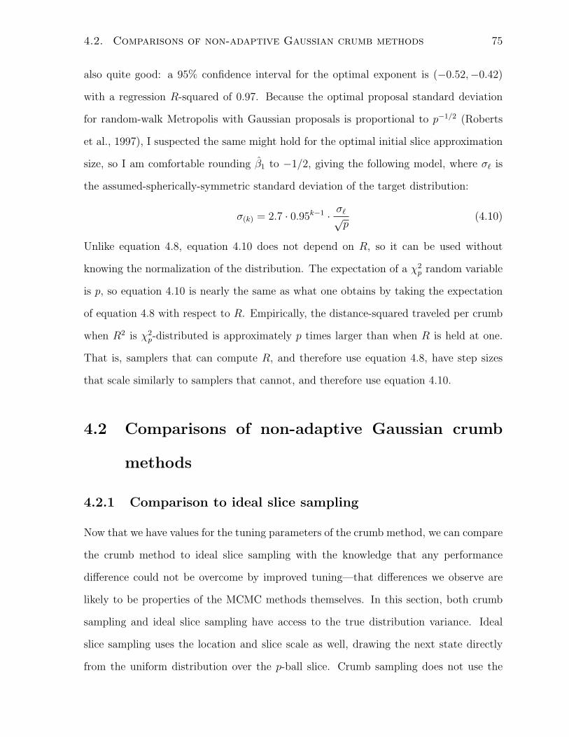
4.2. Comparisons of non-adaptive Gaussian crumb methods 75
also quite good: a 95% confidence interval for the optimal exponent is (−0.52,−0.42)
with a regression R-squared of 0.97. Because the optimal proposal standard deviation
for random-walk Metropolis with Gaussian proposals is proportional to p−1/2 (Roberts
et al., 1997), I suspected the same might hold for the optimal initial slice approximation
size, so I am comfortable rounding β1 to −1/2, giving the following model, where σ` is
the assumed-spherically-symmetric standard deviation of the target distribution:
σ(k) = 2.7 · 0.95k−1 · σ`√p
(4.10)
Unlike equation 4.8, equation 4.10 does not depend on R, so it can be used without
knowing the normalization of the distribution. The expectation of a χ2p random variable
is p, so equation 4.10 is nearly the same as what one obtains by taking the expectation
of equation 4.8 with respect to R. Empirically, the distance-squared traveled per crumb
when R2 is χ2p-distributed is approximately p times larger than when R is held at one.
That is, samplers that can compute R, and therefore use equation 4.8, have step sizes
that scale similarly to samplers that cannot, and therefore use equation 4.10.
4.2 Comparisons of non-adaptive Gaussian crumb
methods
4.2.1 Comparison to ideal slice sampling
Now that we have values for the tuning parameters of the crumb method, we can compare
the crumb method to ideal slice sampling with the knowledge that any performance
difference could not be overcome by improved tuning—that differences we observe are
likely to be properties of the MCMC methods themselves. In this section, both crumb
sampling and ideal slice sampling have access to the true distribution variance. Ideal
slice sampling uses the location and slice scale as well, drawing the next state directly
from the uniform distribution over the p-ball slice. Crumb sampling does not use the
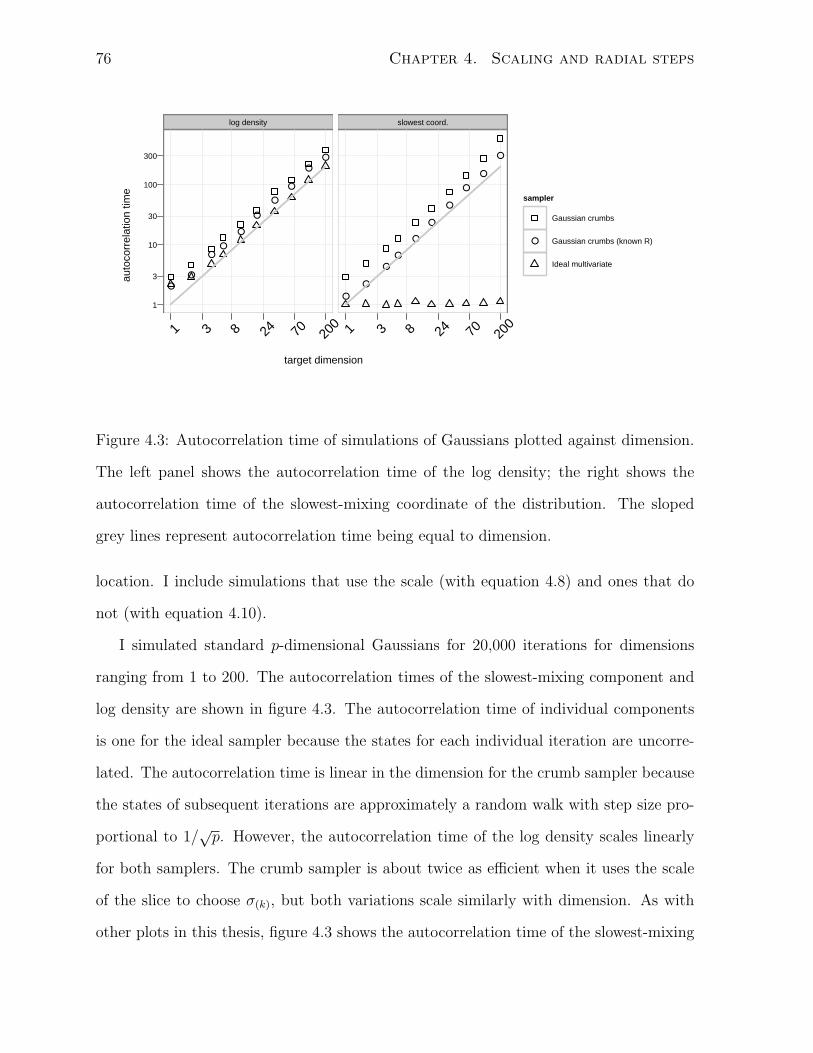
76 Chapter 4. Scaling and radial steps
target dimension
auto
corr
elat
ion
time
1
3
10
30
100
300
log density
●
●
●●
●
●
●
●
●
●
1 3 8 24 70 200
slowest coord.
●
●
●
●
●
●
●
●
●
●
1 3 8 24 70 200
sampler
Gaussian crumbs
● Gaussian crumbs (known R)
Ideal multivariate
Figure 4.3: Autocorrelation time of simulations of Gaussians plotted against dimension.
The left panel shows the autocorrelation time of the log density; the right shows the
autocorrelation time of the slowest-mixing coordinate of the distribution. The sloped
grey lines represent autocorrelation time being equal to dimension.
location. I include simulations that use the scale (with equation 4.8) and ones that do
not (with equation 4.10).
I simulated standard p-dimensional Gaussians for 20,000 iterations for dimensions
ranging from 1 to 200. The autocorrelation times of the slowest-mixing component and
log density are shown in figure 4.3. The autocorrelation time of individual components
is one for the ideal sampler because the states for each individual iteration are uncorre-
lated. The autocorrelation time is linear in the dimension for the crumb sampler because
the states of subsequent iterations are approximately a random walk with step size pro-
portional to 1/√p. However, the autocorrelation time of the log density scales linearly
for both samplers. The crumb sampler is about twice as efficient when it uses the scale
of the slice to choose σ(k), but both variations scale similarly with dimension. As with
other plots in this thesis, figure 4.3 shows the autocorrelation time of the slowest-mixing
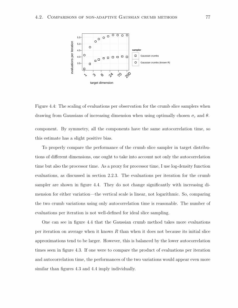
4.2. Comparisons of non-adaptive Gaussian crumb methods 77
target dimension
eval
uatio
ns p
er it
erat
ion
3.5
4.0
4.5
5.0
5.5
●
●
●●
●●
● ● ● ●
1 3 8 24 70 200
sampler
Gaussian crumbs
● Gaussian crumbs (known R)
Figure 4.4: The scaling of evaluations per observation for the crumb slice samplers when
drawing from Gaussians of increasing dimension when using optimally chosen σc and θ.
component. By symmetry, all the components have the same autocorrelation time, so
this estimate has a slight positive bias.
To properly compare the performance of the crumb slice sampler in target distribu-
tions of different dimensions, one ought to take into account not only the autocorrelation
time but also the processor time. As a proxy for processor time, I use log-density function
evaluations, as discussed in section 2.2.3. The evaluations per iteration for the crumb
sampler are shown in figure 4.4. They do not change significantly with increasing di-
mension for either variation—the vertical scale is linear, not logarithmic. So, comparing
the two crumb variations using only autocorrelation time is reasonable. The number of
evaluations per iteration is not well-defined for ideal slice sampling.
One can see in figure 4.4 that the Gaussian crumb method takes more evaluations
per iteration on average when it knows R than when it does not because its initial slice
approximations tend to be larger. However, this is balanced by the lower autocorrelation
times seen in figure 4.3. If one were to compare the product of evaluations per iteration
and autocorrelation time, the performances of the two variations would appear even more
similar than figures 4.3 and 4.4 imply individually.
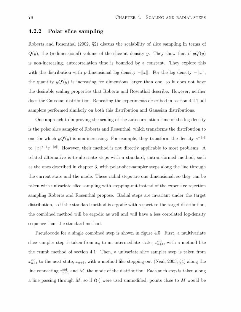
78 Chapter 4. Scaling and radial steps
4.2.2 Polar slice sampling
Roberts and Rosenthal (2002, §2) discuss the scalability of slice sampling in terms of
Q(y), the (p-dimensional) volume of the slice at density y. They show that if yQ′(y)
is non-increasing, autocorrelation time is bounded by a constant. They explore this
with the distribution with p-dimensional log density −‖x‖. For the log density −‖x‖,
the quantity yQ′(y) is increasing for dimensions larger than one, so it does not have
the desirable scaling properties that Roberts and Rosenthal describe. However, neither
does the Gaussian distribution. Repeating the experiments described in section 4.2.1, all
samplers performed similarly on both this distribution and Gaussian distributions.
One approach to improving the scaling of the autocorrelation time of the log density
is the polar slice sampler of Roberts and Rosenthal, which transforms the distribution to
one for which yQ′(y) is non-increasing. For example, they transform the density e−‖x‖
to ‖x‖p−1e−‖x‖. However, their method is not directly applicable to most problems. A
related alternative is to alternate steps with a standard, untransformed method, such
as the ones described in chapter 3, with polar-slice-sampler steps along the line through
the current state and the mode. These radial steps are one dimensional, so they can be
taken with univariate slice sampling with stepping-out instead of the expensive rejection
sampling Roberts and Rosenthal propose. Radial steps are invariant under the target
distribution, so if the standard method is ergodic with respect to the target distribution,
the combined method will be ergodic as well and will have a less correlated log-density
sequence than the standard method.
Pseudocode for a single combined step is shown in figure 4.5. First, a multivariate
slice sampler step is taken from xn to an intermediate state, xstdn+1, with a method like
the crumb method of section 4.1. Then, a univariate slice sampler step is taken from
xstdn+1 to the next state, xn+1, with a method like stepping out (Neal, 2003, §4) along the
line connecting xstdn+1 and M , the mode of the distribution. Each such step is taken along
a line passing through M , so if `(·) were used unmodified, points close to M would be
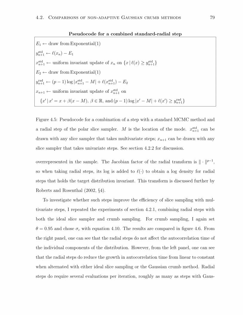
4.2. Comparisons of non-adaptive Gaussian crumb methods 79
Pseudocode for a combined standard-radial step
E1 ← draw from Exponential(1)
ystdn+1 ← `(xn)− E1
xstdn+1 ← uniform invariant update of xn on {x | `(x) ≥ ystd
n+1}
E2 ← draw from Exponential(1)
yradn+1 ← (p− 1) log |xstd
n+1 −M |+ `(xstdn+1)− E2
xn+1 ← uniform invariant update of xstdn+1 on
{x′ |x′ = x+ β(x−M), β ∈ R, and (p− 1) log |x′ −M |+ `(x′) ≥ yradn+1}
Figure 4.5: Pseudocode for a combination of a step with a standard MCMC method and
a radial step of the polar slice sampler. M is the location of the mode. xstdn+1 can be
drawn with any slice sampler that takes multivariate steps; xn+1 can be drawn with any
slice sampler that takes univariate steps. See section 4.2.2 for discussion.
overrepresented in the sample. The Jacobian factor of the radial transform is ‖ · ‖p−1,
so when taking radial steps, its log is added to `(·) to obtain a log density for radial
steps that holds the target distribution invariant. This transform is discussed further by
Roberts and Rosenthal (2002, §4).
To investigate whether such steps improve the efficiency of slice sampling with mul-
tivariate steps, I repeated the experiments of section 4.2.1, combining radial steps with
both the ideal slice sampler and crumb sampling. For crumb sampling, I again set
θ = 0.95 and chose σc with equation 4.10. The results are compared in figure 4.6. From
the right panel, one can see that the radial steps do not affect the autocorrelation time of
the individual components of the distribution. However, from the left panel, one can see
that the radial steps do reduce the growth in autocorrelation time from linear to constant
when alternated with either ideal slice sampling or the Gaussian crumb method. Radial
steps do require several evaluations per iteration, roughly as many as steps with Gaus-
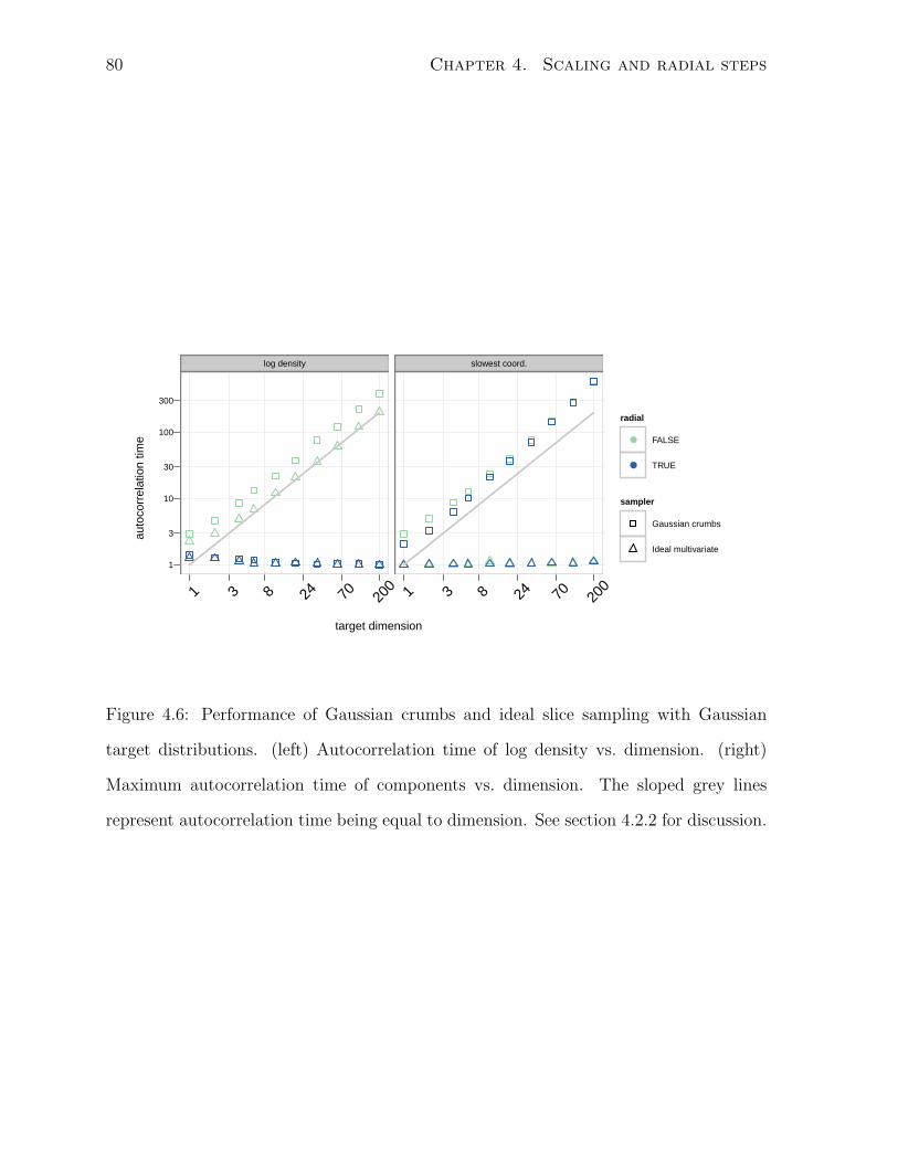
80 Chapter 4. Scaling and radial steps
target dimension
auto
corr
elat
ion
time
1
3
10
30
100
300
log density
1 3 8 24 70 200
slowest coord.
1 3 8 24 70 200
radial
● FALSE
● TRUE
sampler
Gaussian crumbs
Ideal multivariate
Figure 4.6: Performance of Gaussian crumbs and ideal slice sampling with Gaussian
target distributions. (left) Autocorrelation time of log density vs. dimension. (right)
Maximum autocorrelation time of components vs. dimension. The sloped grey lines
represent autocorrelation time being equal to dimension. See section 4.2.2 for discussion.
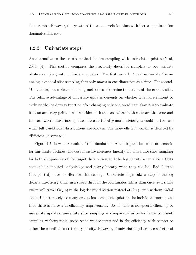
4.2. Comparisons of non-adaptive Gaussian crumb methods 81
sian crumbs. However, the growth of the autocorrelation time with increasing dimension
dominates this cost.
4.2.3 Univariate steps
An alternative to the crumb method is slice sampling with univariate updates (Neal,
2003, §4). This section compares the previously described samplers to two variants
of slice sampling with univariate updates. The first variant, “Ideal univariate,” is an
analogue of ideal slice sampling that only moves in one dimension at a time. The second,
“Univariate,” uses Neal’s doubling method to determine the extent of the current slice.
The relative advantage of univariate updates depends on whether it is more efficient to
evaluate the log density function after changing only one coordinate than it is to evaluate
it at an arbitrary point. I will consider both the case where both costs are the same and
the case where univariate updates are a factor of p more efficient, as could be the case
when full conditional distributions are known. The more efficient variant is denoted by
“Efficient univariate.”
Figure 4.7 shows the results of this simulation. Assuming the less efficient scenario
for univariate updates, the cost measure increases linearly for univariate slice sampling
for both components of the target distribution and the log density when slice extents
cannot be computed analytically, and nearly linearly when they can be. Radial steps
(not plotted) have no effect on this scaling. Univariate steps take a step in the log
density direction p times in a sweep through the coordinates rather than once, so a single
sweep will travel O(√p) in the log density direction instead of O(1), even without radial
steps. Unfortunately, so many evaluations are spent updating the individual coordinates
that there is no overall efficiency improvement. So, if there is no special efficiency to
univariate updates, univariate slice sampling is comparable in performance to crumb
sampling without radial steps when we are interested in the efficiency with respect to
either the coordinates or the log density. However, if univariate updates are a factor of
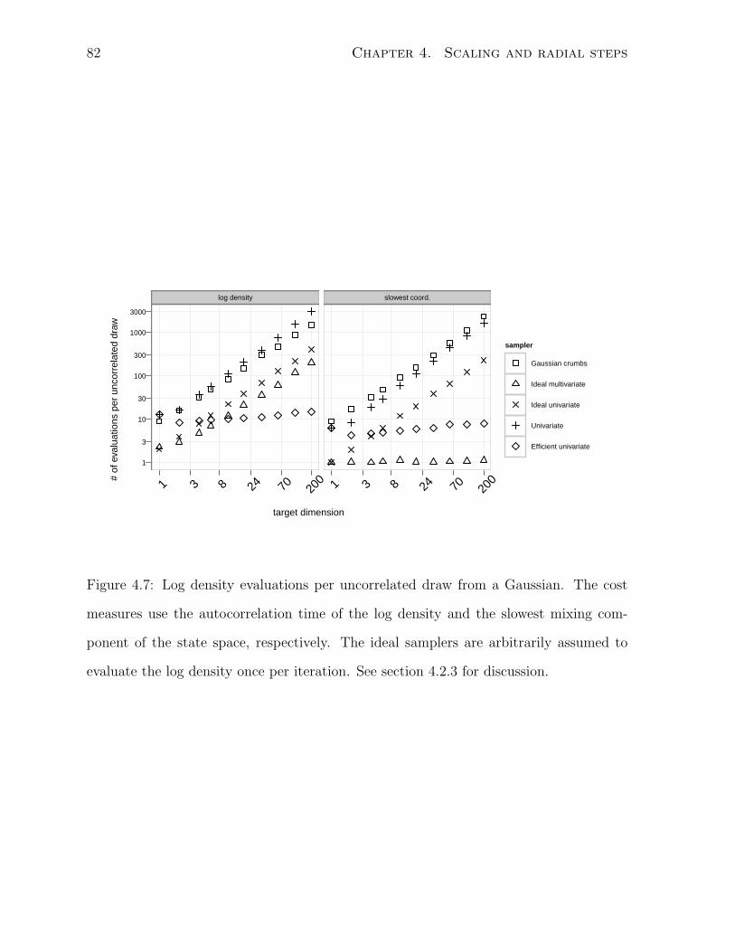
82 Chapter 4. Scaling and radial steps
target dimension
# of
eva
luat
ions
per
unc
orre
late
d dr
aw
1
3
10
30
100
300
1000
3000
log density
1 3 8 24 70 200
slowest coord.
1 3 8 24 70 200
sampler
Gaussian crumbs
Ideal multivariate
Ideal univariate
Univariate
Efficient univariate
Figure 4.7: Log density evaluations per uncorrelated draw from a Gaussian. The cost
measures use the autocorrelation time of the log density and the slowest mixing com-
ponent of the state space, respectively. The ideal samplers are arbitrarily assumed to
evaluate the log density once per iteration. See section 4.2.3 for discussion.
4.2. Comparisons of non-adaptive Gaussian crumb methods 83
p cheaper than arbitrary updates, they have a clear advantage, scaling similarly to ideal
slice sampling with multivariate steps.
4.2.4 Discussion
The Gaussian crumb method is a prototypical slice sampler that uses the shape of a
distribution but not the location of its mode. From the experiments of section 4.2.1, it
seems that the autocorrelation time of components of a distribution sampled with this
method can scale linearly with dimension. One would need to use a method that takes
advantage of the location of the mode to allow for methods where the autocorrelation
time is roughly constant.
However, even if the location of the mode is known, making a method like the ideal
slice sampler plausible, the autocorrelation time of the log density scales linearly with
dimension. As seen in section 4.2.2, the scaling of multivariate step methods can be
improved to a constant when Gaussian crumbs or ideal slice sampling is combined with
the radial steps of the polar slice sampler. The improvements gained changing from
crumb to ideal slice sampling and from adding radial steps are independent. Switching
from crumb to ideal slice sampling improves the coordinate autocorrelation time scaling
from linear to constant, but does not affect the log density autocorrelation time scaling.
Combining crumb or ideal sampling with polar slice sampling improves the log density
autocorrelation time scaling from linear to constant, but does not affect the coordinate
autocorrelation time scaling. If the contours of the target distribution may have sub-
stantially different shapes at different log densities or if one is interested in nonlinear
functions of state, one must take care to achieve convergence in both the log density and
the coordinates.
84 Chapter 4. Scaling and radial steps
4.3 Practical algorithms for radial steps
Radial steps as described in section 4.2.2 are not directly useful because they require the
distribution to have a single, known mode. This section presents a version of radial steps
that relaxes these assumptions.
One could assume there is a single (but unknown) mode and locate it with a mul-
tidimensional optimization routine. Then, steps with any sampler can be alternated
with radial steps of the type described in section 4.2.2. This approach works well for
unimodal distributions. Alternatively, one could run the optimization routine each iter-
ation. Then, the sampler would always take steps toward or away from a local mode. To
maintain invariance of the stationary distribution, the sampler would also have to re-run
the optimization routine and reject a tentatively-accepted proposal whenever the opti-
mization routine does not find the same mode when starting the search at the proposal.
The method to be described in section 4.3.1 is an extension of this idea that allows for
caching of the located maxima.
4.3.1 Radial steps using a gridded state space
A multidimensional optimization each iteration will dominate the cost of the sampler.
One partial solution is to grid the state space and cache the maximum found starting
from each cell. Denote the current state by x0. To find a mode, start the optimization
routine from the center of the grid cell that the current point is in, x′0; denote the resulting
maximum by M0. The next time a mode is needed for any point in the same grid cell,
the maximum is known to be M0, and no optimization need be done. The challenge with
this approach is to identify a grid size, e, small enough for grid cells not to cover multiple
modes but large enough for caching to provide a benefit. Unfortunately, even for very
large grid sizes, the number of grid cells is exponential in the dimension unless one cell
spans the entire state space. So, caching gives the greatest benefit in low dimensional
4.3. Practical algorithms for radial steps 85
state spaces, when the radial steps are least necessary.
Pseudocode for a single gridded radial step is shown in figure 4.8. Subscripts of
0 represent aspects of the current state in Rp; subscripts of 1 represent aspects of a
proposal. The symbol 1p represents a p-dimensional vector of ones, so that ebx/ec +
(e/2) · 1p computes the center of the grid cell with edge length e containing the p-vector
x. The details of maximization are left out; BFGS (Nocedal and Wright, 2006, ch. 6) is a
reasonable method. Stepping out from x0 to find Rmin and Rmax is similar to the stepping
out method described by Neal (2003, §4), but instead of finding a log density less than
yslice in each direction from x0, we search for x such that (p − 1) log ‖M0 − x‖ plus the
log density is less than yslice since we are using polar slice sampling steps. The logged
Jacobian factor, (p − 1) log ‖M0 − x‖, is the same as the one described in section 4.2.2.
Rmin and Rmax are taken to be negative and positive offsets from x0; the endpoints of the
slice approximation are at x0 +Rming0 and x0 +Rmaxg0.
4.3.2 Radial steps using auxiliary variables
This section describes two more variations on radial steps. Like gridded radial steps,
they can be alternated with a standard method as demonstrated in figure 4.5. The first
such method, “Random Pole,” draws a point, c, from a spherically symmetric Gaussian
centered at the current state, x0, with standard deviation σc, a tuning parameter. It
then takes a radial step along the line connecting x0 and c, just as the previous method
takes a radial step along the line connecting x0 and M0. To hold the target distribution
invariant, we must make transitions from x0 to the next state after drawing c equally
likely as transitions from the next state to x0 after drawing c. So, we must multiply
the density for drawing c to the target density, or equivalently, add the log density for
drawing c to the log density. Because this is a radial step, we must also add the Jacobian
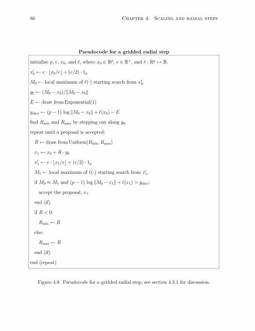
86 Chapter 4. Scaling and radial steps
Pseudocode for a gridded radial step
initialize p, e, x0, and `, where x0 ∈ Rp, e ∈ R+, and ` : Rp 7→ R.
x′0 ← e · bx0/ec+ (e/2) · 1p
M0 ← local maximum of `(·) starting search from x′0.
g0 ← (M0 − x0)/‖M0 − x0‖
E ← draw from Exponential(1)
yslice ← (p− 1) log ‖M0 − x0‖+ `(x0)− E
find Rmin and Rmax by stepping out along g0.
repeat until a proposal is accepted:
R← draw from Uniform(Rmin, Rmax)
x1 ← x0 +R · g0
x′1 ← e · bx1/ec+ (e/2) · 1p
M1 ← local maximum of `(·) starting search from x′1.
if M0 ≈M1 and (p− 1) log ‖M0 − x1‖+ `(x1) > yslice:
accept the proposal, x1.
end (if)
if R < 0:
Rmin ← R
else:
Rmax ← R
end (if)
end (repeat)
Figure 4.8: Pseudocode for a gridded radial step; see section 4.3.1 for discussion.
4.3. Practical algorithms for radial steps 87
term as before. The resulting log density is:
`∗(x) = (p− 1) log ‖c− x‖+ `(x)− 1
2
‖x− c‖2
σ2c
(4.11)
The first term is the Jacobian for the radial transform, the second is the underlying log
density, and the third is the log density for drawing c from x. First, a slice level is drawn:
yslice = `∗(x0)− E, E ∼ Exponential(1) (4.12)
The slice is therefore {x | `∗(x) ≥ yslice}. Stepping out (Neal, 2003, §4) is used to find
the endpoints of the slice approximation on the line {x0 + β(c− x0) | β ∈ R}. Finally, a
univariate slice transition is performed between the endpoints, as described by Neal. This
is similar to the gridded method of section 4.3.1, except the method for finding the line
to search on is different, and the gridded method does not need a density adjustment to
account for the differing probabilities of drawing c, since every proposal that is considered
by that method uses the same local maximum.
A second auxiliary variable method, “1D Pole,” attempts to substitute a one dimen-
sional maximization for the p-dimensional maximization of section 4.3.1. It draws c as
with Random Pole and computes the gradient at c, g = ∇`(c). A parabola through c
and c+ αg, for any nonzero α, has three degrees of freedom. By fixing the log densities
at c and c+αg and the slope at c, which is ‖g‖, we can find Mc, the maximum along the
approximately parabolic cut through `(·). Then, as with Random Pole, 1D Pole takes a
radial step along the line connecting x0 and Mc. It uses the log density:
`∗∗(x) = (p− 1) log ‖Mc − x‖+ `(x)− 1
2
‖x− c‖2
σ2c
(4.13)
Since the transition is along a line connecting x0 and Mc, the Jacobian adjustment
(the first term) must use Mc, but since Mc is determined from c, the adjustment for the
auxiliary variable (the third term) must use c. I choose α to be one somewhat arbitrarily;
the method is not sensitive to its choice on distributions with roughly concentric contours.
In addition, ‖Mc − x0‖ is restricted to be less than 100 · σc, ensuring that floating-point
roundoff does not cause all proposals to be rejected when the gradient is very steep.
88 Chapter 4. Scaling and radial steps
4.3.3 Evaluation on a sequence of Gaussians
This section shows how the methods of section 4.3.1 and 4.3.2 can be combined with
the covariance matching slice sampler of section 3.4 to create a sampler that mixes
efficiently with respect to both the state space and log density. Figure 4.9 compares
four samplers, one implementing the standard covariance matching method and three
where covariance matching steps were alternated with steps described in section 4.3.1
and section 4.3.2. Two variations on gridded radial steps are included: one that uses
conjugate gradient (Fletcher and Reeves, 1964) and one that uses BFGS (Nocedal and
Wright, 2006, ch. 6). The target distributions are a sequence of Gaussians, each with
marginal variances from one to one hundred with uniformly spaced logarithms. For
example, the three-dimensional distribution has marginal variances 1, 10, and 100. The
components of the test distributions are uncorrelated, but since the methods tested are
rotationally invariant except for the minor effect of grid cell alignment when using gridded
radial steps, this does not affect the results. The alignment of the grid and the mode of
the target distributions is such that even with large grid sizes, the number of grid cells
visited is still exponential in the target dimension.
The scale tuning parameter determines σc for covariance matching, σc for 1D Pole
and Random Pole, and e for Grid Cov. Match. The methods’ performance on a given
measure was not sensitive to their tuning parameters, but occasionally different tuning
parameters worked better for different cost measures, so I include two sets of plots. In
general, one need only ensure that σc be at least the same order of magnitude as the
largest marginal standard deviation. Further experiments with tuning parameters chosen
independently had results that were substantially the same as those plotted in figure 4.9.
Whether one optimizes for fast mixing of the log density or the slowest mixing co-
ordinate, the samplers perform similarly with respect to the slowest-mixing coordinates,
with costs scaling approximately quadratically with dimension. This is dominated by
increasing autocorrelation time, which grows approximately as p3/2. As discussed in sec-
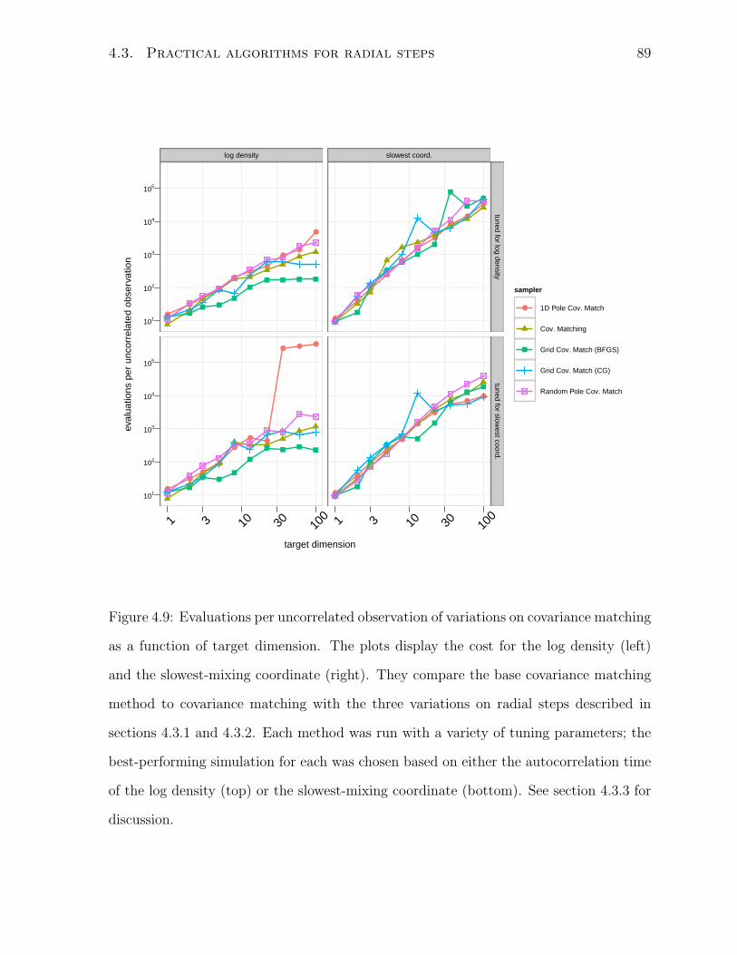
4.3. Practical algorithms for radial steps 89
target dimension
eval
uatio
ns p
er u
ncor
rela
ted
obse
rvat
ion
101
102
103
104
105
101
102
103
104
105
log density
●
●●
●
●●
●
●●
●
●
●●
●
●
● ●
● ● ●
1 3 10 30 100
slowest coord.
●
●
●
●
●
●
●
●●
●
●
●
●
●
●
●
●● ●
●
1 3 10 30 100
tuned for log densitytuned for slow
est coord.
sampler
● 1D Pole Cov. Match
Cov. Matching
Grid Cov. Match (BFGS)
Grid Cov. Match (CG)
Random Pole Cov. Match
Figure 4.9: Evaluations per uncorrelated observation of variations on covariance matching
as a function of target dimension. The plots display the cost for the log density (left)
and the slowest-mixing coordinate (right). They compare the base covariance matching
method to covariance matching with the three variations on radial steps described in
sections 4.3.1 and 4.3.2. Each method was run with a variety of tuning parameters; the
best-performing simulation for each was chosen based on either the autocorrelation time
of the log density (top) or the slowest-mixing coordinate (bottom). See section 4.3.3 for
discussion.
90 Chapter 4. Scaling and radial steps
tion 4.2.2, this would not be better than linear in p even if the target distributions were
spherically-symmetric Gaussians. Evaluations per iteration grow approximately as p1/2;
the relation is somewhat flatter in higher dimensions as the cost of a single optimization
levels out and the elements of the crumb covariance used by covariance matching steps
become dominated by θ-induced shrinkage rather than the parabolic approximations to
the log density.
The cost to obtain an uncorrelated log density is roughly linear in the dimension for all
methods except covariance matching with gridded radial steps, for which it is constant.
The autocorrelation time for the log density in simulations that use either variant of grid-
ded radial steps is effectively one for all dimensions; the increase in cost before the curve
flattens reflects the extra evaluations spent on optimization. It seems that radial steps
must be taken towards a mode for them to have the desired affect. Similar experiments
interleaving gridded radial steps with steps from the oblique hyperrectangle method, de-
scribed in section 3.2.3, and the shrinking rank method, described in section 3.5, suggest
the scaling seen in figure 4.9 is more broadly generalizable.
In high dimensional target spaces, the mixing of coordinates in the target state space
tends to be slower than the mixing of the log density, especially when gridded radial steps
are used. One might prefer to take several steps in the target state space between single
radial steps to minimize the added cost of the radial steps while retaining their benefit.
In the experiment plotted in figure 4.9, the marginal variances are geometrically
spaced. In a supplementary experiment, I simulated several other patterns. Grid Cov.
Match performs well for any pattern. 1D Pole Cov. Match performs comparably well only
when there is at most one marginal variance larger than the smallest ones, such that a
one-dimensional search will be able to nearly attain the maximum log density from any
initial state.
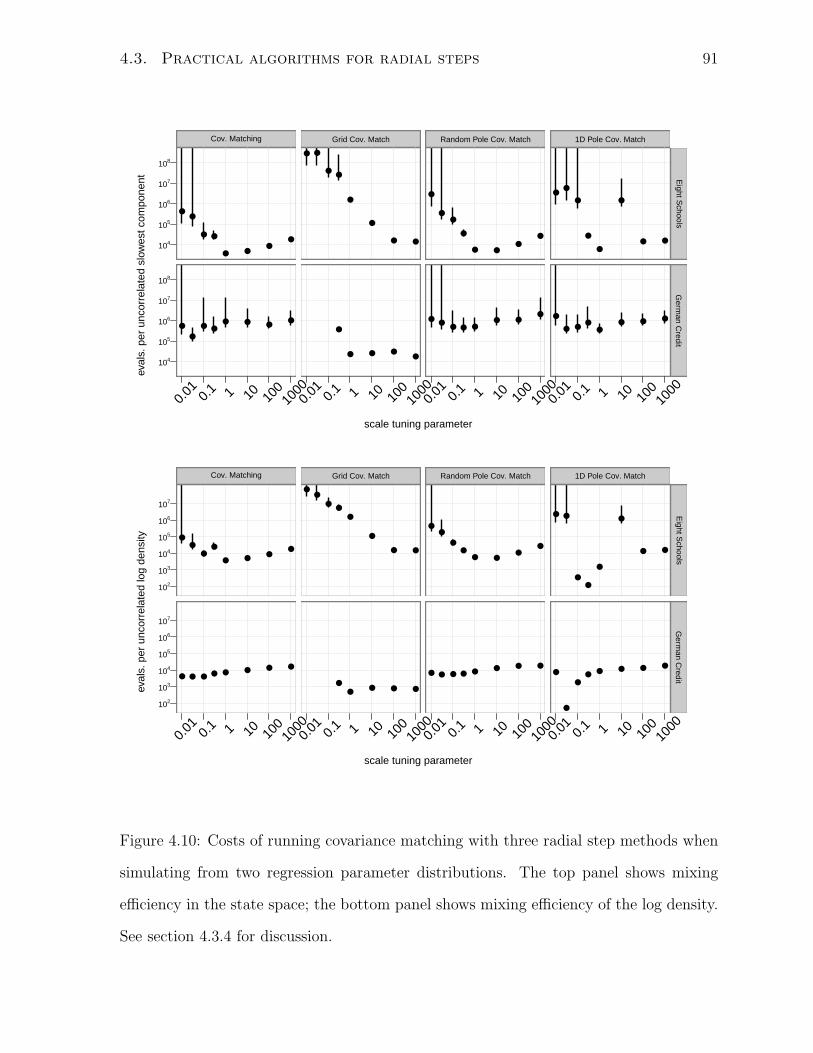
4.3. Practical algorithms for radial steps 91
scale tuning parameter
eval
s. p
er u
ncor
rela
ted
slow
est c
ompo
nent
104
105
106
107
108
104
105
106
107
108
Cov. Matching
●●
● ●
● ●●
●
●
●
● ●● ● ●
●
0.01 0.
1 1 10 100
1000
Grid Cov. Match
● ●
●●
●
●
● ●
● ●
●
●●
0.01 0.
1 1 10 100
1000
Random Pole Cov. Match
●
●●
●
● ●●
●
● ●● ● ●
● ●●
0.01 0.
1 1 10 100
1000
1D Pole Cov. Match
●●
●
●
●
●
● ●
●
● ●●
●● ● ●
0.01 0.
1 1 10 100
1000
Eight S
choolsG
erman C
redit
scale tuning parameter
eval
s. p
er u
ncor
rela
ted
log
dens
ity
102
103
104
105
106
107
102
103
104
105
106
107
Cov. Matching
●●
●●
● ●●
●
● ● ● ● ● ● ● ●
0.01 0.
1 1 10 100
1000
Grid Cov. Match
●●
●●
●
●
● ●
●●
●● ●
0.01 0.
1 1 10 100
1000
Random Pole Cov. Match
●●
●●
● ●●
●
● ● ● ● ● ● ● ●
0.01 0.
1 1 10 100
1000
1D Pole Cov. Match
● ●
●●
●
●
● ●
●
●
●● ● ● ● ●
0.01 0.
1 1 10 100
1000
Eight S
choolsG
erman C
redit
Figure 4.10: Costs of running covariance matching with three radial step methods when
simulating from two regression parameter distributions. The top panel shows mixing
efficiency in the state space; the bottom panel shows mixing efficiency of the log density.
See section 4.3.4 for discussion.

92 Chapter 4. Scaling and radial steps
4.3.4 Evaluation on two regressions
To see whether alternating with radial steps is useful on more realistic distributions, not
just Gaussians, I ran a set of simulations on the Eight Schools and German Credit ex-
amples introduced in section 2.2.2. Figure 4.10 shows the results. As in section 4.3.3,
the scale tuning parameter determines the crumb standard deviations, initial slice ap-
proximation sizes for radial steps, and the grid edge sizes for gridded radial steps, though
the results do not change if they are varied independently. In this experiment, only
the BFGS variant of Grid Cov. Match is included. As with the previous experiment,
Random Pole Cov. Match performs similarly to standard covariance matching. 1D Pole
Cov. Match performs similarly except when precisely tuned. The initial point chosen
for the search, c, must be close enough to the current state, x0, for the gradients at c
and x0 to be similar but far enough away that radial steps can cover a non-negligible
distance. Grid Cov. Match does not depend on its tuning parameter to take large steps;
varying its tuning parameter affects the evaluations per iteration much more than the
autocorrelation time. Grid Cov. Match is generally more efficient with respect to the log
density on German Credit. Since German Credit is a higher-dimensional distribution,
and radial steps are intended to improve scaling with dimension, this is consistent with
earlier results.
Chapter 5
Conclusion
5.1 Contributions
This thesis presents three principal results. First, in chapter 2, I demonstrate a method
for comparing MCMC samplers in more depth and clarity than the dominant methods in
the literature. By using multi-panel graphics rather than tables of numbers, my method
allows researchers to see how new methods compare to established ones in a variety of
conditions, limited by processor time more than other considerations.
Second, in chapter 3, I demonstrate several new variations on slice sampling, all of
which take multivariate steps using only the log density of a target distribution or the
log density and its gradient. Methods based on the eigendecomposition of the sample
covariance matrix perform similarly to Adaptive Metropolis, sampling efficiently on dis-
tributions with highly correlated components and moderate skewness. Like Adaptive
Metropolis, they are globally adaptive, so they may not be appropriate for updating a
subset of the components of the state space. And, like Adaptive Metropolis, they cannot
be used when the target density is of a dimension where operations on the sample covari-
ance are impractical. Since slice samplers can expand and contract slice approximations in
a more straightforward way than Metropolis samplers can expand and contract proposal
93
94 Chapter 5. Conclusion
densities, they are less dependent on tuning. As a result, the eigendecomposition-based
methods are a promising alternative to Adaptive Metropolis.
Later in chapter 3, I demonstrate how the crumb framework can be used to con-
struct samplers that can be embedded in a larger sampling scheme and perform well
when the local curvature of the target distribution is not well-captured by a global co-
variance. These methods, covariance matching and shrinking rank, perform similarly to
the eigendecomposition-based methods but without global adaptation, though they do
require the gradient of the log density, not just the log density. However, they can be
embedded in a larger sampling scheme and are shown to perform well on target distribu-
tions where the correlation structure varies throughout the state space. As a result, they
are applicable to an even wider variety of densities than the eigendecomposition-based
methods. In addition, the shrinking rank method does not store a covariance matrix at
any point, so it is suitable for higher-dimensional distributions than eigendecomposition
methods and covariance matching. This method has displaced all others for my own use
when sampling from distributions with computable gradients.
One way to compute the gradient of a log density function is automatic differentiation;
see Nocedal and Wright (2006, §8.2) for an introduction or Griewank and Walther (2008)
for a more comprehensive treatment. Unfortunately, it is not a mature field. The deriv
R function can compute derivatives of simple expressions, but it is not general enough
for most log densities. At this point, users must still implement gradient functions by
hand. While tedious to write, they can be easily checked for correctness with discrete
approximation.
Finally, in chapter 4, I consider the effect of increasing dimension on the performance
of slice sampling with multivariate steps and demonstrate a practical way to apply the
polar slice sampler, which until now was not practical to implement. I argue that the
number of log density evaluations required to obtain an uncorrelated observation scales
linearly with dimension in most samplers, whether one considers correlation with respect
5.2. Limitations and future work 95
to the components of the distribution or the log density. The scaling behavior of the
log density can be improved by alternating MCMC steps from a gradient-based sampler
like shrinking rank, covariance matching, or reflective slice sampling (Neal, 2003, §7)
with the radial steps of the polar slice sampler. For the common case where the target
distribution does not have a single, known mode, this section shows how steps can use
multidimensional optimization to take radial steps in a way that leaves the target dis-
tribution invariant. If one knows the true shape of the slice, a more difficult condition
than knowing the location of a local mode, scaling with respect to the coordinates can be
improved similarly. These are independent effects; improving one aspect of scaling does
not tend to affect the other.
Together, these results are one step towards the goal of generally applicable Markov
chain Monte Carlo. I hope that other researchers find the methods of model comparison
useful in their own analyses and the sampling methods useful on their own distributions,
ultimately improving the ability of non-specialist end users to analyze data with a broader
range of models than is currently technically feasible.
5.2 Limitations and future work
While the methods described in this thesis are designed to be fairly general, they assume
that the target distribution is continuous. They do not depend on unimodality for cor-
rectness, but they do not make any attempt to move efficiently between modes. They
can, however, be used as part of a larger sampling scheme that uses, for example, Gibbs
sampling to update discrete components and simulated tempering (Marinari and Parisi,
1992) to move between modes.
For some distributions, alternating traditional MCMC steps with gridded radial steps
can improve scaling with respect to the log density. However, efficiency is improved only
if lines through the current state and a local maximum cut across density contours. This

96 Chapter 5. Conclusion
requires that local maxima be identifiable with relatively few function evaluations. In an
attempt to make such steps more efficient and reflective of local structure, I am presently
working on an MCMC method that takes moves along a perturbed gradient, analogously
to the steepest ascent method for multidimensional maximization. I hope to extend
this method to one where sequential steps are orthogonal, analogous to quasi-Newton
methods like BFGS (Nocedal and Wright, 2006, ch. 6).
5.3 Software
• ACTCompare is an R package that compares methods for computing autocor-
relation time, as in section 2.1. It is available at the author’s website, http:
//www.utstat.toronto.edu/mthompson.
• SamplerCompare is an R package for comparing MCMC samplers, as described
in section 2.3. It includes R implementations of the covariance matching method,
univariate sampling along eigenvectors, and the oblique hyperrectangle method and
a C implementation of the shrinking rank method. It is available from CRAN at
http://cran.r-project.org/web/packages/SamplerCompare/index.html.
• A demonstration implementation of covariance matching with gridded radial steps
is available at http://www.utstat.toronto.edu/mthompson/gridded-radial.R.
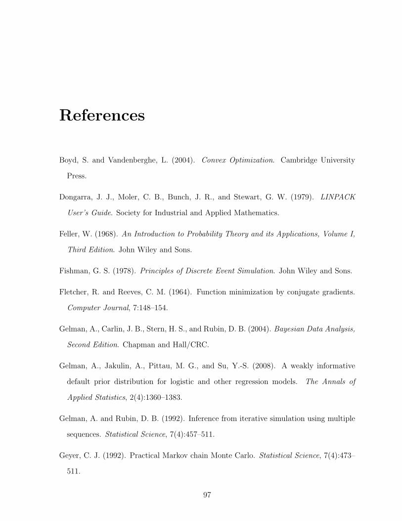
References
Boyd, S. and Vandenberghe, L. (2004). Convex Optimization. Cambridge University
Press.
Dongarra, J. J., Moler, C. B., Bunch, J. R., and Stewart, G. W. (1979). LINPACK
User’s Guide. Society for Industrial and Applied Mathematics.
Feller, W. (1968). An Introduction to Probability Theory and its Applications, Volume I,
Third Edition. John Wiley and Sons.
Fishman, G. S. (1978). Principles of Discrete Event Simulation. John Wiley and Sons.
Fletcher, R. and Reeves, C. M. (1964). Function minimization by conjugate gradients.
Computer Journal, 7:148–154.
Gelman, A., Carlin, J. B., Stern, H. S., and Rubin, D. B. (2004). Bayesian Data Analysis,
Second Edition. Chapman and Hall/CRC.
Gelman, A., Jakulin, A., Pittau, M. G., and Su, Y.-S. (2008). A weakly informative
default prior distribution for logistic and other regression models. The Annals of
Applied Statistics, 2(4):1360–1383.
Gelman, A. and Rubin, D. B. (1992). Inference from iterative simulation using multiple
sequences. Statistical Science, 7(4):457–511.
Geyer, C. J. (1992). Practical Markov chain Monte Carlo. Statistical Science, 7(4):473–
511.
97
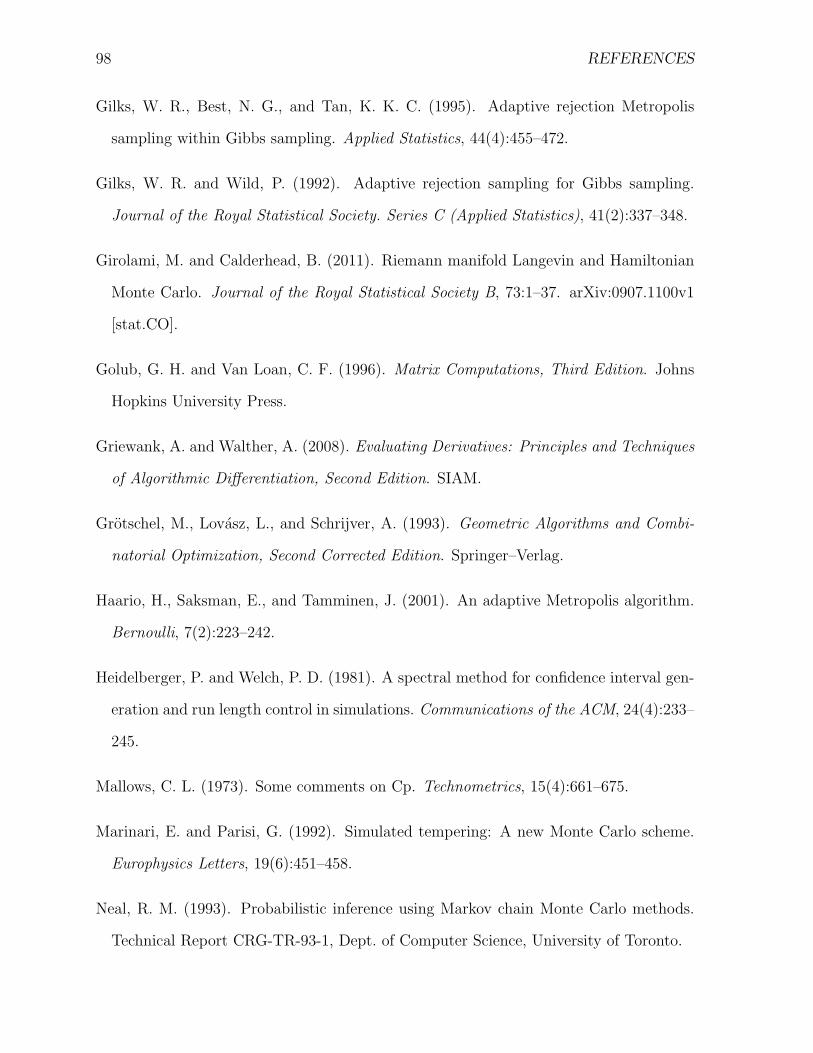
98 REFERENCES
Gilks, W. R., Best, N. G., and Tan, K. K. C. (1995). Adaptive rejection Metropolis
sampling within Gibbs sampling. Applied Statistics, 44(4):455–472.
Gilks, W. R. and Wild, P. (1992). Adaptive rejection sampling for Gibbs sampling.
Journal of the Royal Statistical Society. Series C (Applied Statistics), 41(2):337–348.
Girolami, M. and Calderhead, B. (2011). Riemann manifold Langevin and Hamiltonian
Monte Carlo. Journal of the Royal Statistical Society B, 73:1–37. arXiv:0907.1100v1
[stat.CO].
Golub, G. H. and Van Loan, C. F. (1996). Matrix Computations, Third Edition. Johns
Hopkins University Press.
Griewank, A. and Walther, A. (2008). Evaluating Derivatives: Principles and Techniques
of Algorithmic Differentiation, Second Edition. SIAM.
Grotschel, M., Lovasz, L., and Schrijver, A. (1993). Geometric Algorithms and Combi-
natorial Optimization, Second Corrected Edition. Springer–Verlag.
Haario, H., Saksman, E., and Tamminen, J. (2001). An adaptive Metropolis algorithm.
Bernoulli, 7(2):223–242.
Heidelberger, P. and Welch, P. D. (1981). A spectral method for confidence interval gen-
eration and run length control in simulations. Communications of the ACM, 24(4):233–
245.
Mallows, C. L. (1973). Some comments on Cp. Technometrics, 15(4):661–675.
Marinari, E. and Parisi, G. (1992). Simulated tempering: A new Monte Carlo scheme.
Europhysics Letters, 19(6):451–458.
Neal, R. M. (1993). Probabilistic inference using Markov chain Monte Carlo methods.
Technical Report CRG-TR-93-1, Dept. of Computer Science, University of Toronto.
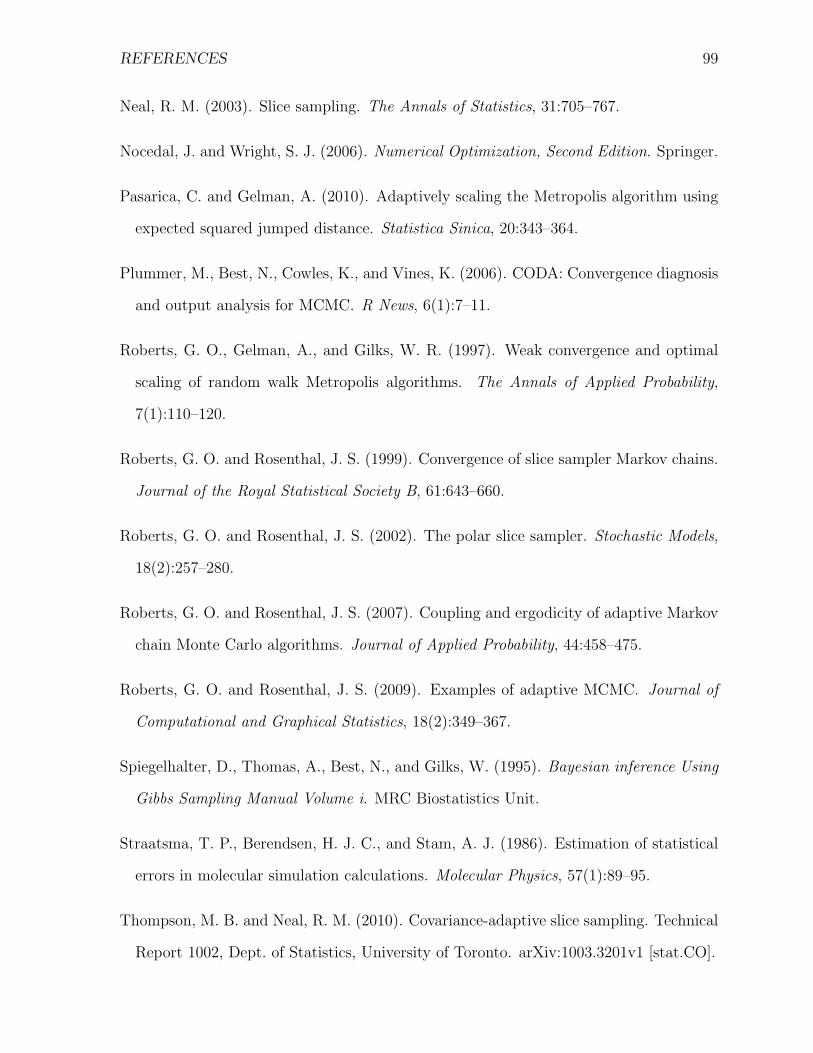
REFERENCES 99
Neal, R. M. (2003). Slice sampling. The Annals of Statistics, 31:705–767.
Nocedal, J. and Wright, S. J. (2006). Numerical Optimization, Second Edition. Springer.
Pasarica, C. and Gelman, A. (2010). Adaptively scaling the Metropolis algorithm using
expected squared jumped distance. Statistica Sinica, 20:343–364.
Plummer, M., Best, N., Cowles, K., and Vines, K. (2006). CODA: Convergence diagnosis
and output analysis for MCMC. R News, 6(1):7–11.
Roberts, G. O., Gelman, A., and Gilks, W. R. (1997). Weak convergence and optimal
scaling of random walk Metropolis algorithms. The Annals of Applied Probability,
7(1):110–120.
Roberts, G. O. and Rosenthal, J. S. (1999). Convergence of slice sampler Markov chains.
Journal of the Royal Statistical Society B, 61:643–660.
Roberts, G. O. and Rosenthal, J. S. (2002). The polar slice sampler. Stochastic Models,
18(2):257–280.
Roberts, G. O. and Rosenthal, J. S. (2007). Coupling and ergodicity of adaptive Markov
chain Monte Carlo algorithms. Journal of Applied Probability, 44:458–475.
Roberts, G. O. and Rosenthal, J. S. (2009). Examples of adaptive MCMC. Journal of
Computational and Graphical Statistics, 18(2):349–367.
Spiegelhalter, D., Thomas, A., Best, N., and Gilks, W. (1995). Bayesian inference Using
Gibbs Sampling Manual Volume i. MRC Biostatistics Unit.
Straatsma, T. P., Berendsen, H. J. C., and Stam, A. J. (1986). Estimation of statistical
errors in molecular simulation calculations. Molecular Physics, 57(1):89–95.
Thompson, M. B. and Neal, R. M. (2010). Covariance-adaptive slice sampling. Technical
Report 1002, Dept. of Statistics, University of Toronto. arXiv:1003.3201v1 [stat.CO].

100 REFERENCES
Tibbits, M., Groendyke, C., and Haran, M. (2010). Automated factor slice sampling.
Talk at 2010 Joint Statistical Meetings in Vancouver.
Wei, W. W. S. (2006). Time Series Analysis: Univariate and Multivariate Methods,
Second Edition. Pearson/Addison Wesley.