slides . by
DESCRIPTION
SLIDES . BY. John Loucks St . Edward’s University. Chapter 4 Introduction to Probability. Experiments, Counting Rules, and Assigning Probabilities. Events and Their Probability. Some Basic Relationships of Probability. Conditional Probability. Bayes’ Theorem. - PowerPoint PPT PresentationTRANSCRIPT
1 1 Slide Slide© 2015 Cengage Learning. All Rights Reserved. May not be scanned, copied
or duplicated, or posted to a publicly accessible website, in whole or in part.
SLIDES . BY
John LoucksSt. Edward’sUniversity
...........

2 2 Slide Slide© 2015 Cengage Learning. All Rights Reserved. May not be scanned, copied
or duplicated, or posted to a publicly accessible website, in whole or in part.
Chapter 4 Introduction to Probability
Experiments, Counting Rules, and Assigning Probabilities
Events and Their Probability Some Basic Relationships of Probability Conditional Probability Bayes’ Theorem

3 3 Slide Slide© 2015 Cengage Learning. All Rights Reserved. May not be scanned, copied
or duplicated, or posted to a publicly accessible website, in whole or in part.
Uncertainties
Managers often base their decisions on an analysis of uncertainties such as the following:
What are the chances that sales will decreaseif we increase prices?
What is the likelihood a new assembly methodwill increase productivity?
What are the odds that a new investment willbe profitable?

4 4 Slide Slide© 2015 Cengage Learning. All Rights Reserved. May not be scanned, copied
or duplicated, or posted to a publicly accessible website, in whole or in part.
Probability
Probability is a numerical measure of the likelihood that an event will occur.
Probability values are always assigned on a scale from 0 to 1.
A probability near zero indicates an event is quite unlikely to occur.
A probability near one indicates an event is almost certain to occur.

5 5 Slide Slide© 2015 Cengage Learning. All Rights Reserved. May not be scanned, copied
or duplicated, or posted to a publicly accessible website, in whole or in part.
Probability as a Numerical Measureof the Likelihood of Occurrence
0 1.5
Increasing Likelihood of Occurrence
Probability:
The eventis veryunlikelyto occur.
The occurrenceof the event is
just as likely asit is unlikely.
The eventis almostcertain
to occur.

6 6 Slide Slide© 2015 Cengage Learning. All Rights Reserved. May not be scanned, copied
or duplicated, or posted to a publicly accessible website, in whole or in part.
Statistical Experiments
In statistics, the notion of an experiment differs somewhat from that of an experiment in the physical sciences.
In statistical experiments, probability determines outcomes.
Even though the experiment is repeated in exactly the same way, an entirely different outcome may occur.
For this reason, statistical experiments are some- times called random experiments.

7 7 Slide Slide© 2015 Cengage Learning. All Rights Reserved. May not be scanned, copied
or duplicated, or posted to a publicly accessible website, in whole or in part.
An Experiment and Its Sample Space
An experiment is any process that generates well- defined outcomes.
The sample space for an experiment is the set of all experimental outcomes.
An experimental outcome is also called a sample point.

8 8 Slide Slide© 2015 Cengage Learning. All Rights Reserved. May not be scanned, copied
or duplicated, or posted to a publicly accessible website, in whole or in part.
An Experiment and Its Sample Space
Experiment
Toss a coinInspection a partConduct a sales callRoll a diePlay a football game
Experiment Outcomes
Head, tailDefective, non-defectivePurchase, no purchase1, 2, 3, 4, 5, 6Win, lose, tie

9 9 Slide Slide© 2015 Cengage Learning. All Rights Reserved. May not be scanned, copied
or duplicated, or posted to a publicly accessible website, in whole or in part.
Bradley has invested in two stocks, Markley Oil
and Collins Mining. Bradley has determined that the
possible outcomes of these investments three months
from now are as follows. Investment Gain or Loss in 3 Months (in $1000s)
Markley Oil Collins Mining 10 5 0-20
8-2
Example: Bradley Investments
An Experiment and Its Sample Space

10 10 Slide Slide© 2015 Cengage Learning. All Rights Reserved. May not be scanned, copied
or duplicated, or posted to a publicly accessible website, in whole or in part.
A Counting Rule for Multiple-Step Experiments
If an experiment consists of a sequence of k steps in which there are n1 possible results for the first step,
n2 possible results for the second step, and so on,
then the total number of experimental outcomes is given by (n1)(n2) . . . (nk).
A helpful graphical representation of a multiple-step experiment is a tree diagram.

11 11 Slide Slide© 2015 Cengage Learning. All Rights Reserved. May not be scanned, copied
or duplicated, or posted to a publicly accessible website, in whole or in part.
Bradley Investments can be viewed as a two-step
experiment. It involves two stocks, each with a set of
experimental outcomes.Markley Oil: n1 = 4Collins Mining: n2 = 2Total Number of Experimental Outcomes: n1n2 = (4)(2) = 8
A Counting Rule for Multiple-Step Experiments
Example: Bradley Investments

12 12 Slide Slide© 2015 Cengage Learning. All Rights Reserved. May not be scanned, copied
or duplicated, or posted to a publicly accessible website, in whole or in part.
Tree Diagram
Gain 5Gain 5
Gain 8Gain 8
Gain 8Gain 8
Gain 10Gain 10
Gain 8Gain 8
Gain 8Gain 8
Lose 20Lose 20
Lose 2Lose 2
Lose 2Lose 2
Lose 2Lose 2
Lose 2Lose 2
EvenEven
Markley Oil(Stage 1)
Collins Mining(Stage 2)
ExperimentalOutcomes
(10, 8) Gain $18,000
(10, -2) Gain $8,000
(5, 8) Gain $13,000
(5, -2) Gain $3,000
(0, 8) Gain $8,000
(0, -2) Lose $2,000
(-20, 8) Lose $12,000
(-20, -2) Lose $22,000
Example: Bradley Investments

13 13 Slide Slide© 2015 Cengage Learning. All Rights Reserved. May not be scanned, copied
or duplicated, or posted to a publicly accessible website, in whole or in part.
A second useful counting rule enables us to count
the number of experimental outcomes when n objects
are to be selected from a set of N objects.
Counting Rule for Combinations
CN
nN
n N nnN
!
!( )!
Number of Combinations of N Objects Taken n at a Time
where: N! = N(N - 1)(N - 2) . . . (2)(1) n! = n(n - 1)(n - 2) . . . (2)(1) 0! = 1

14 14 Slide Slide© 2015 Cengage Learning. All Rights Reserved. May not be scanned, copied
or duplicated, or posted to a publicly accessible website, in whole or in part.
Number of Permutations of N Objects Taken n at a Time
where: N! = N(N - 1)(N - 2) . . . (2)(1) n! = n(n - 1)(n - 2) . . . (2)(1) 0! = 1
P nN
nN
N nnN
!!
( )!
Counting Rule for Permutations
A third useful counting rule enables us to count
the number of experimental outcomes when n objects are to be selected from a set of N
objects,where the order of selection is important.

15 15 Slide Slide© 2015 Cengage Learning. All Rights Reserved. May not be scanned, copied
or duplicated, or posted to a publicly accessible website, in whole or in part.
Assigning Probabilities
Basic Requirements for Assigning Probabilities
1. The probability assigned to each experimental outcome must be between 0 and 1, inclusively.
0 < P(Ei) < 1 for all i
where: Ei is the ith experimental outcome and P(Ei) is its probability

16 16 Slide Slide© 2015 Cengage Learning. All Rights Reserved. May not be scanned, copied
or duplicated, or posted to a publicly accessible website, in whole or in part.
Assigning Probabilities
Basic Requirements for Assigning Probabilities
2. The sum of the probabilities for all experimental outcomes must equal 1.
P(E1) + P(E2) + . . . + P(En) = 1
where:n is the number of experimental outcomes
17 17 Slide Slide© 2015 Cengage Learning. All Rights Reserved. May not be scanned, copied
or duplicated, or posted to a publicly accessible website, in whole or in part.
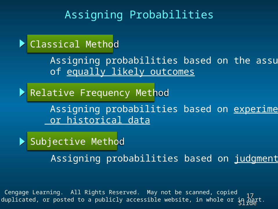
Assigning Probabilities
Classical Method
Relative Frequency Method
Subjective Method
Assigning probabilities based on the assumption of equally likely outcomes
Assigning probabilities based on experimentation or historical data
Assigning probabilities based on judgment

18 18 Slide Slide© 2015 Cengage Learning. All Rights Reserved. May not be scanned, copied
or duplicated, or posted to a publicly accessible website, in whole or in part.
Classical Method
If an experiment has n possible outcomes, the
classical method would assign a probability of 1/n
to each outcome.Experiment: Rolling a die
Sample Space: S = {1, 2, 3, 4, 5, 6}
Probabilities: Each sample point has a 1/6 chance of occurring
Example: Rolling a Die
19 19 Slide Slide© 2015 Cengage Learning. All Rights Reserved. May not be scanned, copied
or duplicated, or posted to a publicly accessible website, in whole or in part.
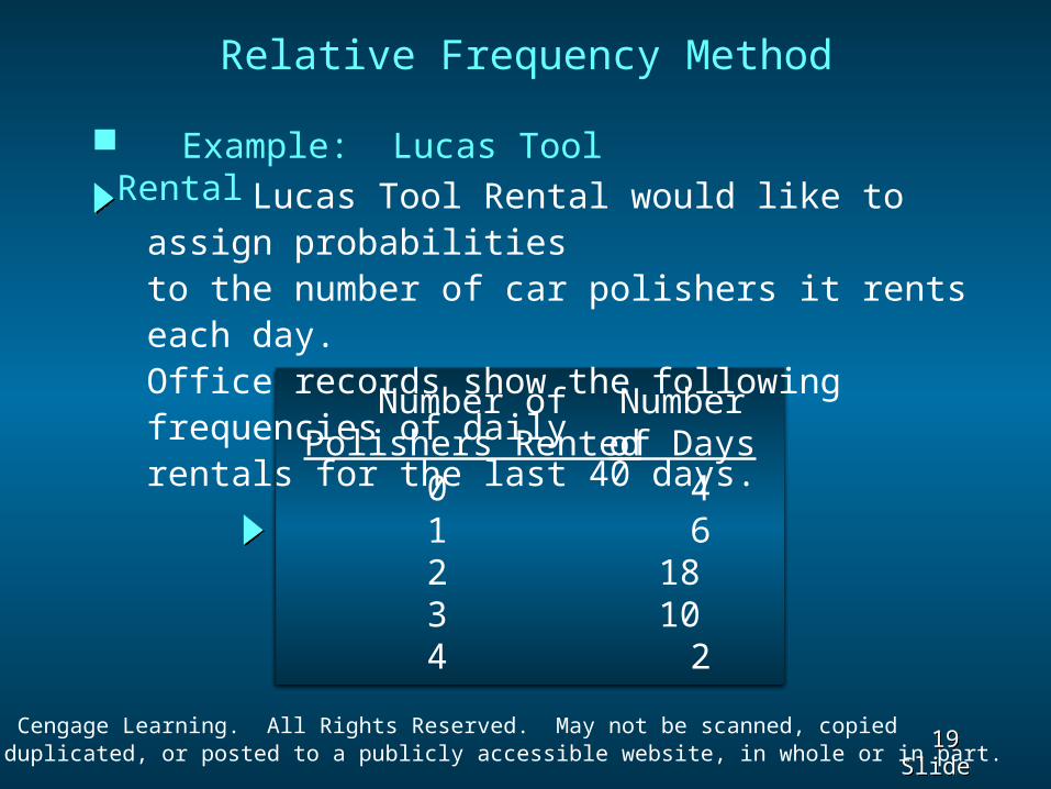
Relative Frequency Method
Number ofPolishers Rented
Numberof Days
01234
4 61810 2
Lucas Tool Rental would like to assign probabilitiesto the number of car polishers it rents each day. Office records show the following frequencies of dailyrentals for the last 40 days.
Example: Lucas Tool Rental

20 20 Slide Slide© 2015 Cengage Learning. All Rights Reserved. May not be scanned, copied
or duplicated, or posted to a publicly accessible website, in whole or in part.
Each probability assignment is given by dividing
the frequency (number of days) by the total frequency
(total number of days).
Relative Frequency Method
4/40
ProbabilityNumber of
Polishers RentedNumberof Days
01234
4 61810 240
.10 .15 .45 .25 .051.00
Example: Lucas Tool Rental
21 21 Slide Slide© 2015 Cengage Learning. All Rights Reserved. May not be scanned, copied
or duplicated, or posted to a publicly accessible website, in whole or in part.
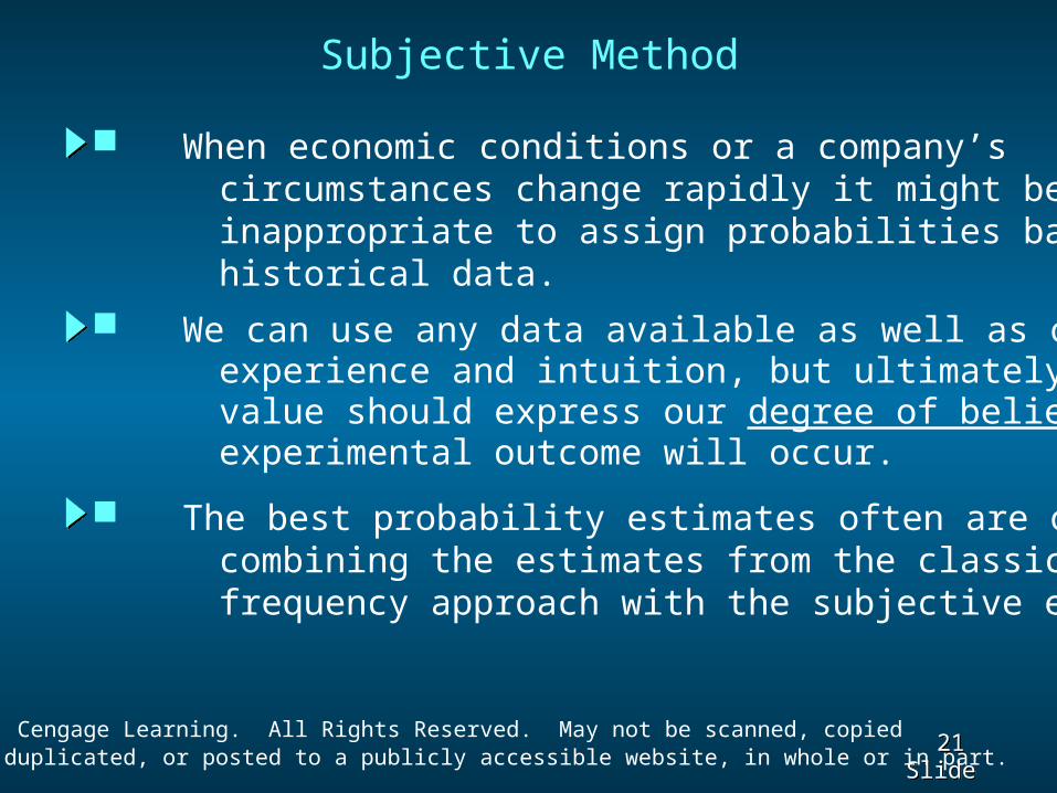
Subjective Method
When economic conditions or a company’s circumstances change rapidly it might be inappropriate to assign probabilities based solely on historical data. We can use any data available as well as our experience and intuition, but ultimately a probability value should express our degree of belief that the experimental outcome will occur.
The best probability estimates often are obtained by combining the estimates from the classical or relative frequency approach with the subjective estimate.

22 22 Slide Slide© 2015 Cengage Learning. All Rights Reserved. May not be scanned, copied
or duplicated, or posted to a publicly accessible website, in whole or in part.
Subjective Method
An analyst made the following probability estimates.
Exper. OutcomeNet Gain or Loss Probability(10, 8)(10, -2)(5, 8)(5, -2)(0, 8)(0, -2)(-20, 8)(-20, -2)
$18,000 Gain $8,000 Gain $13,000 Gain $3,000 Gain $8,000 Gain $2,000 Loss $12,000 Loss $22,000 Loss
.20
.08
.16
.26
.10
.12
.02
.06
Example: Bradley Investments
1.00

23 23 Slide Slide© 2015 Cengage Learning. All Rights Reserved. May not be scanned, copied
or duplicated, or posted to a publicly accessible website, in whole or in part.
An event is a collection of sample points.
The probability of any event is equal to the sum of the probabilities of the sample points in the event.
If we can identify all the sample points of an experiment and assign a probability to each, we can compute the probability of an event.
Events and Their Probabilities
24 24 Slide Slide© 2015 Cengage Learning. All Rights Reserved. May not be scanned, copied
or duplicated, or posted to a publicly accessible website, in whole or in part.
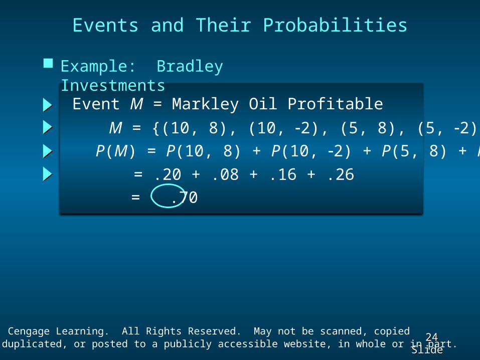
Events and Their Probabilities
Event M = Markley Oil Profitable
M = {(10, 8), (10, -2), (5, 8), (5, -2)}P(M) = P(10, 8) + P(10, -2) + P(5, 8) + P(5, -2)
= .20 + .08 + .16 + .26= .70
Example: Bradley Investments

25 25 Slide Slide© 2015 Cengage Learning. All Rights Reserved. May not be scanned, copied
or duplicated, or posted to a publicly accessible website, in whole or in part.
Events and Their Probabilities
Event C = Collins Mining Profitable
C = {(10, 8), (5, 8), (0, 8), (-20, 8)}P(C) = P(10, 8) + P(5, 8) + P(0, 8) + P(-20, 8)
= .20 + .16 + .10 + .02= .48
Example: Bradley Investments

26 26 Slide Slide© 2015 Cengage Learning. All Rights Reserved. May not be scanned, copied
or duplicated, or posted to a publicly accessible website, in whole or in part.
Some Basic Relationships of Probability
There are some basic probability relationships that
can be used to compute the probability of an event
without knowledge of all the sample point probabilities.
Complement of an Event
Intersection of Two Events
Mutually Exclusive Events
Union of Two Events

27 27 Slide Slide© 2015 Cengage Learning. All Rights Reserved. May not be scanned, copied
or duplicated, or posted to a publicly accessible website, in whole or in part.
The complement of A is denoted by Ac.
The complement of event A is defined to be the event consisting of all sample points that are not in A.
Complement of an Event
Event A AcSampleSpace SSampleSpace S
VennDiagra
m
28 28 Slide Slide© 2015 Cengage Learning. All Rights Reserved. May not be scanned, copied
or duplicated, or posted to a publicly accessible website, in whole or in part.
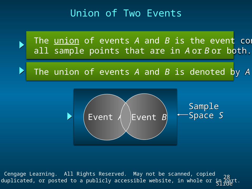
The union of events A and B is denoted by A B
The union of events A and B is the event containing all sample points that are in A or B or both.
Union of Two Events
SampleSpace SSampleSpace SEvent A Event B

29 29 Slide Slide© 2015 Cengage Learning. All Rights Reserved. May not be scanned, copied
or duplicated, or posted to a publicly accessible website, in whole or in part.
Union of Two Events
Event M = Markley Oil Profitable
Event C = Collins Mining Profitable
M C = Markley Oil Profitable or Collins Mining Profitable (or both)
M C = {(10, 8), (10, -2), (5, 8), (5, -2), (0, 8), (-20, 8)}
P(M C) = P(10, 8) + P(10, -2) + P(5, 8) + P(5, -2) + P(0, 8) + P(-20, 8)
= .20 + .08 + .16 + .26 + .10 + .02
= .82
Example: Bradley Investments
30 30 Slide Slide© 2015 Cengage Learning. All Rights Reserved. May not be scanned, copied
or duplicated, or posted to a publicly accessible website, in whole or in part.
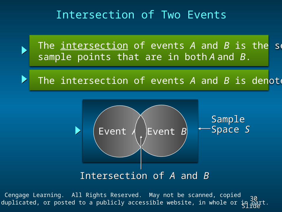
The intersection of events A and B is denoted by A
The intersection of events A and B is the set of all sample points that are in both A and B.
SampleSpace SSampleSpace SEvent A Event B
Intersection of Two Events
Intersection of A and BIntersection of A and B

31 31 Slide Slide© 2015 Cengage Learning. All Rights Reserved. May not be scanned, copied
or duplicated, or posted to a publicly accessible website, in whole or in part.
Intersection of Two Events
Event M = Markley Oil Profitable
Event C = Collins Mining Profitable
M C = Markley Oil Profitable and Collins Mining Profitable
M C = {(10, 8), (5, 8)}
P(M C) = P(10, 8) + P(5, 8)
= .20 + .16
= .36
Example: Bradley Investments

32 32 Slide Slide© 2015 Cengage Learning. All Rights Reserved. May not be scanned, copied
or duplicated, or posted to a publicly accessible website, in whole or in part.
The addition law provides a way to compute the probability of event A, or B, or both A and B occurring.
Addition Law
The law is written as:
P(A B) = P(A) + P(B) - P(A B
33 33 Slide Slide© 2015 Cengage Learning. All Rights Reserved. May not be scanned, copied
or duplicated, or posted to a publicly accessible website, in whole or in part.
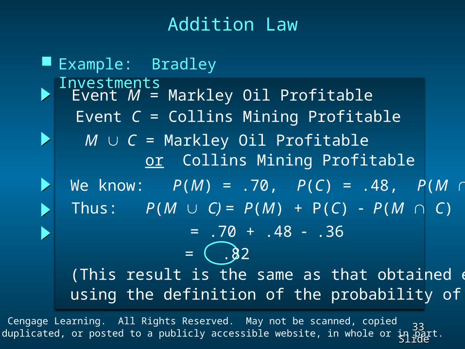
Event M = Markley Oil ProfitableEvent C = Collins Mining Profitable
M C = Markley Oil Profitable or Collins Mining Profitable
We know: P(M) = .70, P(C) = .48, P(M C) = .36
Thus: P(M C) = P(M) + P(C) - P(M C)
= .70 + .48 - .36= .82
Addition Law
(This result is the same as that obtained earlierusing the definition of the probability of an event.)
Example: Bradley Investments

34 34 Slide Slide© 2015 Cengage Learning. All Rights Reserved. May not be scanned, copied
or duplicated, or posted to a publicly accessible website, in whole or in part.
Mutually Exclusive Events
Two events are said to be mutually exclusive if the events have no sample points in common.
Two events are mutually exclusive if, when one event occurs, the other cannot occur.
SampleSpace SSampleSpace SEvent A Event B

35 35 Slide Slide© 2015 Cengage Learning. All Rights Reserved. May not be scanned, copied
or duplicated, or posted to a publicly accessible website, in whole or in part.
Mutually Exclusive Events
If events A and B are mutually exclusive, P(A B = 0.
The addition law for mutually exclusive events is:
P(A B) = P(A) + P(B)
There is no need toinclude “- P(A B”

36 36 Slide Slide© 2015 Cengage Learning. All Rights Reserved. May not be scanned, copied
or duplicated, or posted to a publicly accessible website, in whole or in part.
The probability of an event given that another event has occurred is called a conditional probability.
A conditional probability is computed as follows :
The conditional probability of A given B is denoted by P(A|B).
Conditional Probability
( )( | )
( )P A B
P A BP B

37 37 Slide Slide© 2015 Cengage Learning. All Rights Reserved. May not be scanned, copied
or duplicated, or posted to a publicly accessible website, in whole or in part.
Event M = Markley Oil Profitable
Event C = Collins Mining Profitable
We know: P(M C) = .36, P(M) = .70
Thus:
Conditional Probability
( ) .36( | ) .5143
( ) .70P C M
P C MP M
= Collins Mining Profitable given Markley Oil Profitable
( | )P C M
Example: Bradley Investments

38 38 Slide Slide© 2015 Cengage Learning. All Rights Reserved. May not be scanned, copied
or duplicated, or posted to a publicly accessible website, in whole or in part.
Multiplication Law
The multiplication law provides a way to compute the probability of the intersection of two events.
The law is written as:
P(A B) = P(B)P(A|B)

39 39 Slide Slide© 2015 Cengage Learning. All Rights Reserved. May not be scanned, copied
or duplicated, or posted to a publicly accessible website, in whole or in part.
Event M = Markley Oil ProfitableEvent C = Collins Mining Profitable
We know: P(M) = .70, P(C|M) = .5143
Multiplication Law
M C = Markley Oil Profitable and Collins Mining Profitable
Thus: P(M C) = P(M)P(M|C)= (.70)(.5143)= .36
(This result is the same as that obtained earlierusing the definition of the probability of an event.)
Example: Bradley Investments

40 40 Slide Slide© 2015 Cengage Learning. All Rights Reserved. May not be scanned, copied
or duplicated, or posted to a publicly accessible website, in whole or in part.
Joint Probability Table
Collins MiningProfitable (C) Not Profitable (Cc)Markley Oil
Profitable (M)
Not Profitable (Mc)
Total .48 .52
Total
.70
.30
1.00
.36 .34
.12 .18
Joint Probabilities(appear in the
bodyof the table)
Marginal Probabilities(appear in the
marginsof the table)

41 41 Slide Slide© 2015 Cengage Learning. All Rights Reserved. May not be scanned, copied
or duplicated, or posted to a publicly accessible website, in whole or in part.
Independent Events
If the probability of event A is not changed by the existence of event B, we would say that events A and B are independent.
Two events A and B are independent if:
P(A|B) = P(A) P(B|A) = P(B)or

42 42 Slide Slide© 2015 Cengage Learning. All Rights Reserved. May not be scanned, copied
or duplicated, or posted to a publicly accessible website, in whole or in part.
The multiplication law also can be used as a test to see if two events are independent.
The law is written as:
P(A B) = P(A)P(B)
Multiplication Lawfor Independent Events

43 43 Slide Slide© 2015 Cengage Learning. All Rights Reserved. May not be scanned, copied
or duplicated, or posted to a publicly accessible website, in whole or in part.
Event M = Markley Oil ProfitableEvent C = Collins Mining Profitable
We know: P(M C) = .36, P(M) = .70, P(C) = .48 But: P(M)P(C) = (.70)(.48) = .34, not .36
Are events M and C independent?DoesP(M C) = P(M)P(C) ?
Hence: M and C are not independent.
Example: Bradley Investments
Multiplication Lawfor Independent Events
44 44 Slide Slide© 2015 Cengage Learning. All Rights Reserved. May not be scanned, copied
or duplicated, or posted to a publicly accessible website, in whole or in part.
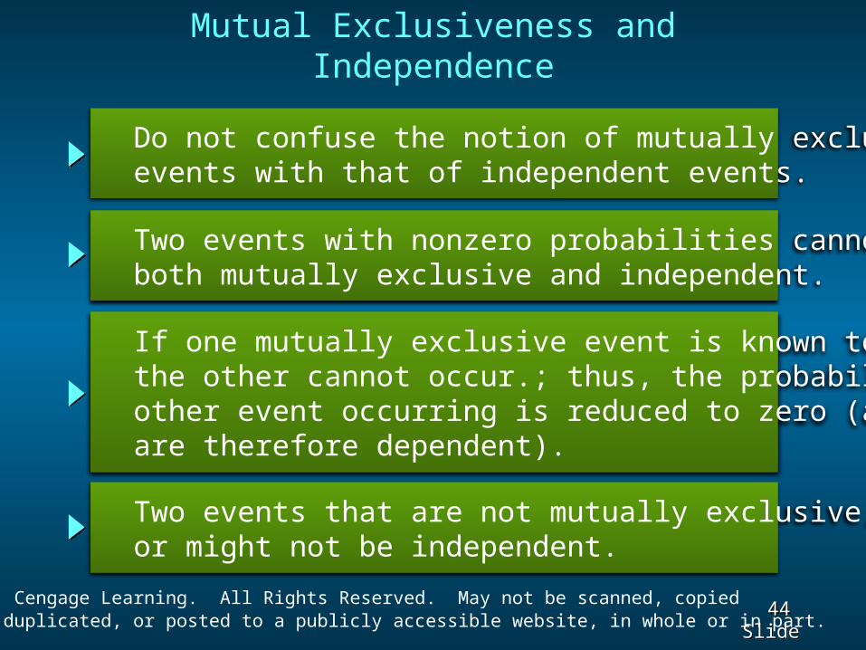
Do not confuse the notion of mutually exclusive events with that of independent events.
Two events with nonzero probabilities cannot be both mutually exclusive and independent.
If one mutually exclusive event is known to occur, the other cannot occur.; thus, the probability of the other event occurring is reduced to zero (and they are therefore dependent).
Mutual Exclusiveness and Independence
Two events that are not mutually exclusive, might or might not be independent.

45 45 Slide Slide© 2015 Cengage Learning. All Rights Reserved. May not be scanned, copied
or duplicated, or posted to a publicly accessible website, in whole or in part.
Bayes’ Theorem
NewInformation
Applicationof Bayes’Theorem
PosteriorProbabilities
PriorProbabilities
Often we begin probability analysis with initial or prior probabilities.
Then, from a sample, special report, or a product test we obtain some additional information. Given this information, we calculate revised or posterior probabilities.
Bayes’ theorem provides the means for revising the prior probabilities.

46 46 Slide Slide© 2015 Cengage Learning. All Rights Reserved. May not be scanned, copied
or duplicated, or posted to a publicly accessible website, in whole or in part.
A proposed shopping center will provide strong
competition for downtown businesses like L. S.Clothiers. If the shopping center is built, the
ownerof L. S. Clothiers feels it would be best to
relocate tothe shopping center.
Bayes’ Theorem
Example: L. S. Clothiers
The shopping center cannot be built unless azoning change is approved by the town council.The planning board must first make a recommendation, for or against the zoning change,to the council.

47 47 Slide Slide© 2015 Cengage Learning. All Rights Reserved. May not be scanned, copied
or duplicated, or posted to a publicly accessible website, in whole or in part.
Let:
Prior Probabilities
A1 = town council approves the zoning change
A2 = town council disapproves the change
P(A1) = .7, P(A2) = .3
Using subjective judgment:
Example: L. S. Clothiers

48 48 Slide Slide© 2015 Cengage Learning. All Rights Reserved. May not be scanned, copied
or duplicated, or posted to a publicly accessible website, in whole or in part.
The planning board has recommended against
the zoning change. Let B denote the event of a
negative recommendation by the planning board.
New Information
Example: L. S. Clothiers
Given that B has occurred, should L. S. Clothiers
revise the probabilities that the town council will
approve or disapprove the zoning change?
49 49 Slide Slide© 2015 Cengage Learning. All Rights Reserved. May not be scanned, copied
or duplicated, or posted to a publicly accessible website, in whole or in part.
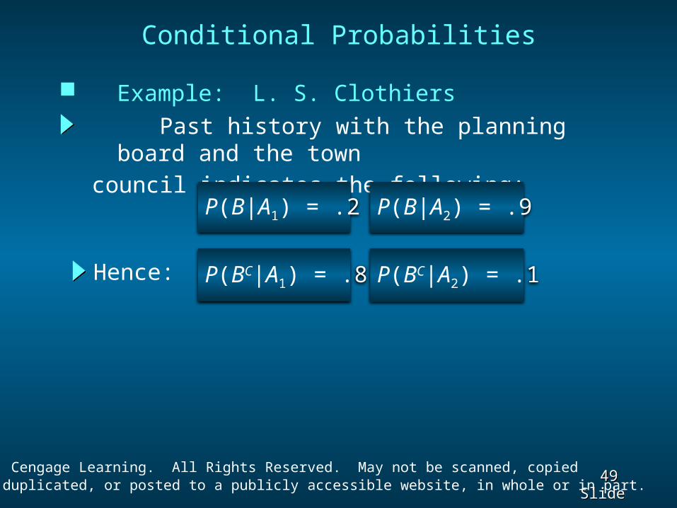
Past history with the planning board and the town
council indicates the following:
Conditional Probabilities
P(B|A1) = .2 P(B|A2) = .9
P(BC|A1) = .8 P(BC|A2) = .1Hence:
Example: L. S. Clothiers

50 50 Slide Slide© 2015 Cengage Learning. All Rights Reserved. May not be scanned, copied
or duplicated, or posted to a publicly accessible website, in whole or in part.
P(Bc|A1) = .8P(Bc|A1) = .8P(A1) = .7P(A1) = .7
P(A2) = .3P(A2) = .3
P(B|A2) = .9P(B|A2) = .9
P(Bc|A2) = .1P(Bc|A2) = .1
P(B|A1) = .2P(B|A1) = .2 P(A1 B) = .14P(A1 B) = .14
P(A2 B) = .27P(A2 B) = .27
P(A2 Bc) = .03P(A2 Bc) = .03
P(A1 Bc) = .56P(A1 Bc) = .56
Town Council Planning Board ExperimentalOutcomes
Tree Diagram
Example: L. S. Clothiers
1.00

51 51 Slide Slide© 2015 Cengage Learning. All Rights Reserved. May not be scanned, copied
or duplicated, or posted to a publicly accessible website, in whole or in part.
Bayes’ Theorem
1 1 2 2
( ) ( | )( | )
( ) ( | ) ( ) ( | ) ... ( ) ( | )i i
in n
P A P B AP A B
P A P B A P A P B A P A P B A
To find the posterior probability that event Ai will occur given that event B has occurred, we apply Bayes’ theorem.
Bayes’ theorem is applicable when the events for which we want to compute posterior probabilities are mutually exclusive and their union is the entire sample space.

52 52 Slide Slide© 2015 Cengage Learning. All Rights Reserved. May not be scanned, copied
or duplicated, or posted to a publicly accessible website, in whole or in part.
Given the planning board’s recommendation not
to approve the zoning change, we revise the prior
probabilities as follows: 1 11
1 1 2 2
( ) ( | )( | )
( ) ( | ) ( ) ( | )P A P B A
P A BP A P B A P A P B A
(. )(. )(. )(. ) (. )(. )
7 27 2 3 9
Posterior Probabilities
= .34
Example: L. S. Clothiers
53 53 Slide Slide© 2015 Cengage Learning. All Rights Reserved. May not be scanned, copied
or duplicated, or posted to a publicly accessible website, in whole or in part.
The planning board’s recommendation is good
news for L. S. Clothiers. The posterior probability of
the town council approving the zoning change is .34
compared to a prior probability of .70.
Example: L. S. Clothiers
Posterior Probabilities

54 54 Slide Slide© 2015 Cengage Learning. All Rights Reserved. May not be scanned, copied
or duplicated, or posted to a publicly accessible website, in whole or in part.
Bayes’ Theorem: Tabular Approach
Example: L. S. Clothiers
Column 1 - The mutually exclusive events for which posterior probabilities are desired.
Column 2 - The prior probabilities for the events.
Column 3 - The conditional probabilities of the new information given each event.
Prepare the following three columns:• Step 1

55 55 Slide Slide© 2015 Cengage Learning. All Rights Reserved. May not be scanned, copied
or duplicated, or posted to a publicly accessible website, in whole or in part.
(1) (2) (3) (4) (5)
Events
Ai
PriorProbabilities
P(Ai)
ConditionalProbabilities
P(B|Ai)
A1
A2
.7
.3
1.0
.2
.9
Example: L. S. Clothiers
Bayes’ Theorem: Tabular Approach
• Step 1
56 56 Slide Slide© 2015 Cengage Learning. All Rights Reserved. May not be scanned, copied
or duplicated, or posted to a publicly accessible website, in whole or in part.
Bayes’ Theorem: Tabular Approach
Column 4 Compute the joint probabilities for each event
andthe new information B by using the multiplicationlaw.
Prepare the fourth column:
Multiply the prior probabilities in column 2 by the corresponding conditional probabilities in column 3. That is, P(Ai IB) = P(Ai) P(B|Ai).
Example: L. S. Clothiers• Step 2

57 57 Slide Slide© 2015 Cengage Learning. All Rights Reserved. May not be scanned, copied
or duplicated, or posted to a publicly accessible website, in whole or in part.
(1) (2) (3) (4) (5)
Events
Ai
PriorProbabilities
P(Ai)
ConditionalProbabilities
P(B|Ai)
A1
A2
.7
.3
1.0
.2
.9
.14
.27
JointProbabilities
P(Ai I B)
.7 x .2
Example: L. S. Clothiers
Bayes’ Theorem: Tabular Approach
• Step 2

58 58 Slide Slide© 2015 Cengage Learning. All Rights Reserved. May not be scanned, copied
or duplicated, or posted to a publicly accessible website, in whole or in part.
• Step 2 (continued)
We see that there is a .14 probability of the towncouncil approving the zoning change and anegative recommendation by the planning board.
Example: L. S. Clothiers
Bayes’ Theorem: Tabular Approach
There is a .27 probability of the town councildisapproving the zoning change and a negativerecommendation by the planning board.

59 59 Slide Slide© 2015 Cengage Learning. All Rights Reserved. May not be scanned, copied
or duplicated, or posted to a publicly accessible website, in whole or in part.
• Step 3
Sum the joint probabilities in Column 4. Thesum is the probability of the new information,P(B). The sum .14 + .27 shows an overallprobability of .41 of a negative recommendationby the planning board.
Example: L. S. Clothiers
Bayes’ Theorem: Tabular Approach

60 60 Slide Slide© 2015 Cengage Learning. All Rights Reserved. May not be scanned, copied
or duplicated, or posted to a publicly accessible website, in whole or in part.
(1) (2) (3) (4) (5)
Events
Ai
PriorProbabilities
P(Ai)
ConditionalProbabilities
P(B|Ai)
A1
A2
.7
.3
1.0
.2
.9
.14
.27
JointProbabilities
P(Ai I B)
P(B) = .41
Example: L. S. Clothiers
Bayes’ Theorem: Tabular Approach
• Step 3

61 61 Slide Slide© 2015 Cengage Learning. All Rights Reserved. May not be scanned, copied
or duplicated, or posted to a publicly accessible website, in whole or in part.
)(
)()|(
BP
BAPBAP i
i
Bayes’ Theorem: Tabular Approach
Prepare the fifth column:
Column 5 Compute the posterior probabilities using
thebasic relationship of conditional probability.
Example: L. S. Clothiers• Step 4
The joint probabilities P(Ai I B) are in column 4
and the probability P(B) is the sum of column 4.

62 62 Slide Slide© 2015 Cengage Learning. All Rights Reserved. May not be scanned, copied
or duplicated, or posted to a publicly accessible website, in whole or in part.
(1) (2) (3) (4) (5)
Events
Ai
PriorProbabilities
P(Ai)
ConditionalProbabilities
P(B|Ai)
A1
A2
.7
.3
1.0
.2
.9
.14
.27
JointProbabilities
P(Ai I B)
P(B) = .41
.14/.41
PosteriorProbabilities
P(Ai |B)
.3415
.6585
1.0000
Example: L. S. Clothiers
Bayes’ Theorem: Tabular Approach
• Step 4

63 63 Slide Slide© 2015 Cengage Learning. All Rights Reserved. May not be scanned, copied
or duplicated, or posted to a publicly accessible website, in whole or in part.
End of Chapter 4