7/30/2018

1

Reconstruction

across imaging

modalities: MRI

Brad Sutton

bsutton@Illinois.edu

Bioengineering and Beckman

Institute

Introduction to Spins and Classical MRI Physics

Spinning proton == SPIN

Spinning proton has a magnetic moment ::

Classical Description: Behaves as a bar magnet.

Most MRI scans are

looking at hydrogen

nucleus.

This is good: Body is

mostly water H2O

Other nuclei are available

in MRI:13C, 19F, 23Na,

others

H+

N

S

Sample outside the MRI magnet, spins

randomly oriented.

7/30/2018

2

N

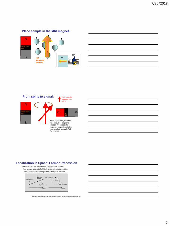
Place sample in the MRI magnet…

Net

Magnetic

Moment

MRIS

Static Field

ON

From spins to signal:

When tipped away from the

main field, then begins to

precess. Precesses at a

frequency proportional to the

magnetic field strength. At 3

T = 128 MHz

Net magnetic

moment from

spins

N

S

Static Field

ON N S

RF

Localization in Space: Larmor PrecessionSince frequency is proportional magnetic field strength

if we apply a magnetic field that varies with spatial position,

the precession frequency varies with spatial position.

x Position

BMag. FieldStrength

Low Frequency

High Frequency

x Position

High Frequency

Low Frequency

Object

From Noll: fMRI Primer: http://fmri.research.umich.edu/documents/fmri_primer.pdf

7/30/2018

3

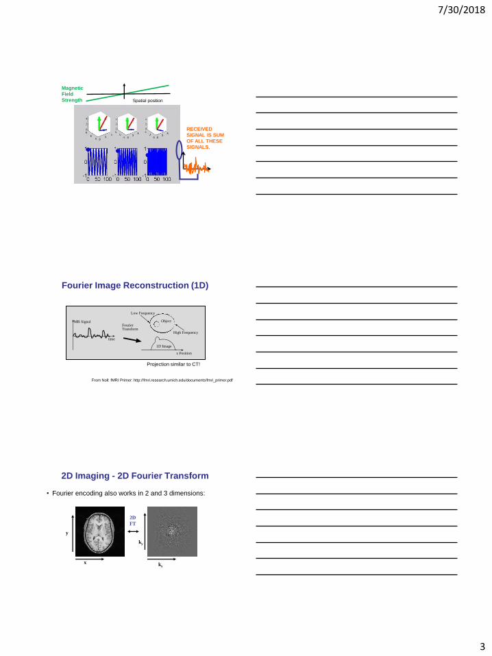
Magnetic

Field

Strength Spatial position

RECEIVED

SIGNAL IS SUM

OF ALL THESE

SIGNALS.

Fourier Image Reconstruction (1D)

MR SignalFourierTransform

x Position

High Frequency

Low Frequency

Object

1D Image

time

Projection similar to CT!

From Noll: fMRI Primer: http://fmri.research.umich.edu/documents/fmri_primer.pdf

2D Imaging - 2D Fourier Transform

• Fourier encoding also works in 2 and 3 dimensions:

2D

FT

x kx

ky

y

7/30/2018

4

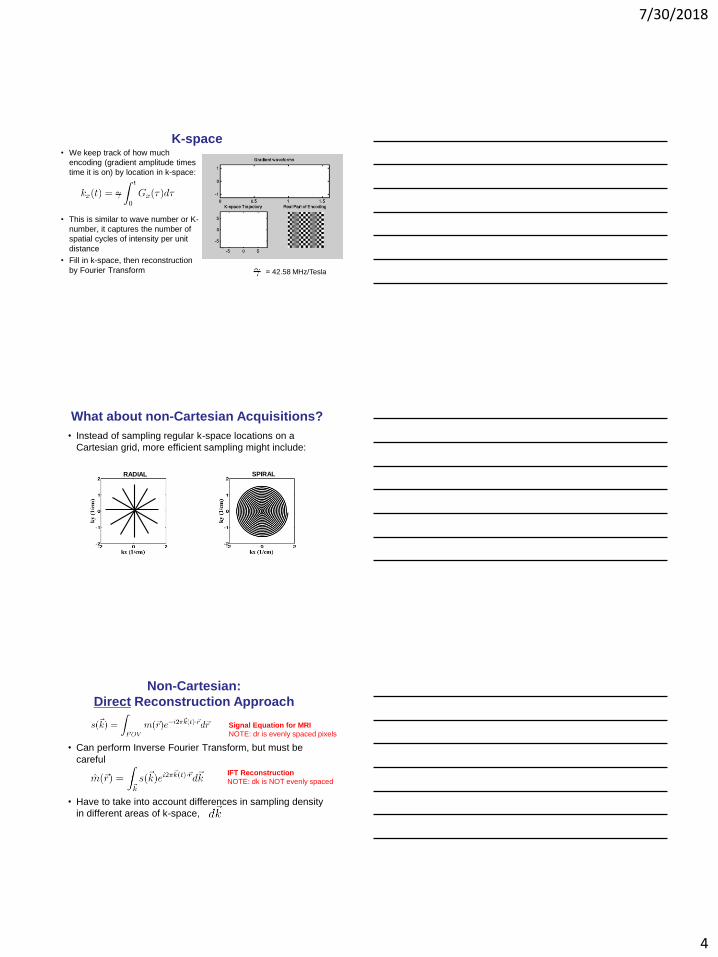
K-space• We keep track of how much

encoding (gradient amplitude times

time it is on) by location in k-space:

• This is similar to wave number or K-

number, it captures the number of

spatial cycles of intensity per unit

distance

• Fill in k-space, then reconstruction

by Fourier Transform = 42.58 MHz/Tesla

What about non-Cartesian Acquisitions?

• Instead of sampling regular k-space locations on a

Cartesian grid, more efficient sampling might include:

RADIAL SPIRAL

Non-Cartesian:

Direct Reconstruction Approach

• Can perform Inverse Fourier Transform, but must be

careful

• Have to take into account differences in sampling density

in different areas of k-space,

Signal Equation for MRI

NOTE: dr is evenly spaced pixels

IFT Reconstruction

NOTE: dk is NOT evenly spaced

7/30/2018

5

Sample Density

Compensation• Density compensation function

(DCF) represents the differential

area element for each sample.

• Can calculate DCF in many

ways:

– Voronoi area (shown)

– Analytical formulation of gradient

– Jacobian of time/k-space

transformation

– PSF optimizationDCF Calculation via Voronoi diagram for 4 shot spiral, showing sampling locations and differential area elements

With DCF, now can perform recon• Inverse Discrete Space Fourier Transform

• But for large problems, we would like to

use the Fast Fourier Transform (FFT).

– k is still not equally sampled on regular grid:

requirement for FFT!

• What are the options?

Density Compensation

Function

Simply INTERPOLATE onto regular grid and then use FFT?

We will show that we can do better than that with GRIDDING!

Gridding: Fast, accurate, direct recon

• Steps in Gridding1. Density compensate k-space data w(k)*s(k)

2. Convolution with a fixed-width blurring kernel to

fill in continuous sampling of k-space

3. Resample data at uniform Cartesian locations

4. Inverse FFT

5. Deapodization: Eliminate the effect of the fixed

kernel interpolator.

Convolution in k-space is multiplication in image

space, so we can remove the effect of the

convolution by dividing by the FT of the kernel in

image space.

Jackson, et al. IEEE Trans Med Imaging. 1991;10(3):473-8.

1D simulation from: Noll and Sutton, ISMRM Educational Session, 2003.

7/30/2018

6

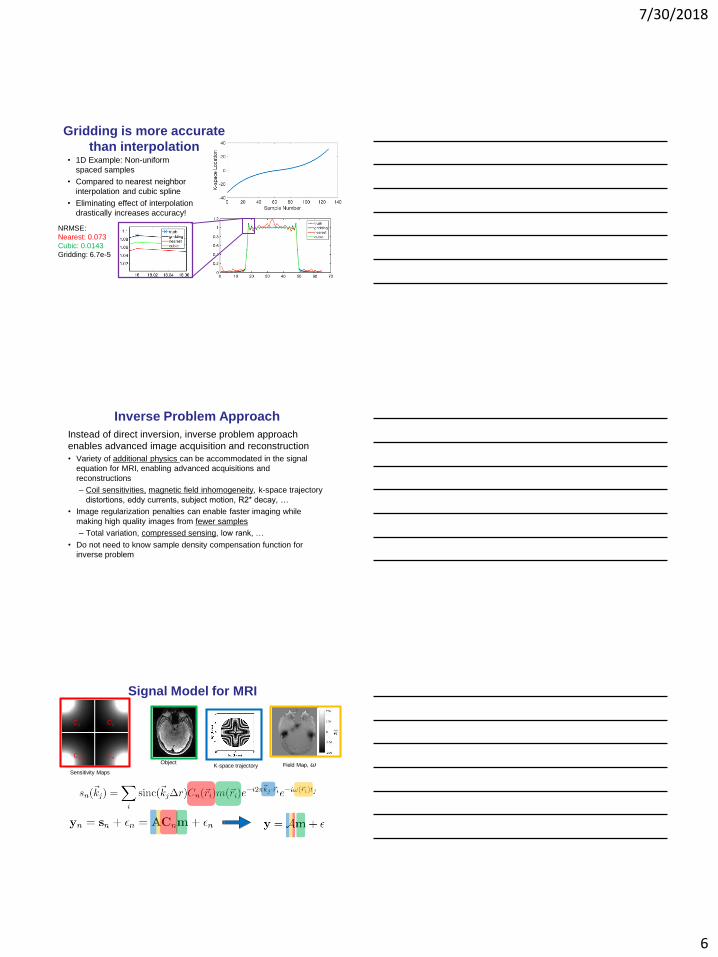
Gridding is more accurate

than interpolation• 1D Example: Non-uniform

spaced samples

• Compared to nearest neighbor

interpolation and cubic spline

• Eliminating effect of interpolation

drastically increases accuracy!

NRMSE:

Nearest: 0.073

Cubic: 0.0143

Gridding: 6.7e-5

Inverse Problem Approach

Instead of direct inversion, inverse problem approach

enables advanced image acquisition and reconstruction

• Variety of additional physics can be accommodated in the signal

equation for MRI, enabling advanced acquisitions and

reconstructions

– Coil sensitivities, magnetic field inhomogeneity, k-space trajectory

distortions, eddy currents, subject motion, R2* decay, …

• Image regularization penalties can enable faster imaging while

making high quality images from fewer samples

– Total variation, compressed sensing, low rank, …

• Do not need to know sample density compensation function for

inverse problem

Signal Model for MRI

Sensitivity Maps

Object Field Map, 𝜔K-space trajectory

C1 C2

C3 C4

7/30/2018

7

Inverse problem approach• In complex-valued MRI, noise is complex Gaussian.

• Makes statistics easier than other modalities

• Can use least squares approaches for image

reconstruction

• Can add regularization to help with the usually ill-

conditioned problem, provides prior information on

acceptable solutions, through some function

Example: Magnetic Field Inhomogeneity

Image Distortion

Distortion depends on

K-space trajectory and

bandwidth (how fast

sample k-space).

(ppm)B0

Incorporation of the field

inhomogeneity map into the

inverse problem to correct

for it.

Air/tissue interfaces cause

most magnetic field

disruptions, for example

around sinuses. Air/Tissue interfaces

can cause up to ~1 KHz

off-resonance at 3 T

Example: Magnetic Field Inhomogeneity

Holtrop and Sutton. J Medical imaging. 3(2): 023501 (2016).

Sutton, et al. J Magn Reson Imaging. 32:1228 (2010)

High Resolution (0.8 mm isotropic)

diffusion MRI, b=1000 s/mm2

Field MapCorrectedUncorrected

Dynamic Speech

Imaging with

FLASH. Air/tissue

susceptibility can

be 1.2 kHz at 3 T.

Uncorrected Corrected

7/30/2018

8

Regularization and Constraints

• Image reconstruction is ill-conditioned problem

– Sample only the minimum data (or less) that we need to keep

scan time short

– Push the spatial resolution higher → signal-to-noise lower

– Non-ideal experimental conditions

• Magnetic field map changed since measurement

• Coil sensitivies changed

• K-space trajectory deviations

• Must enforce prior information on the solution in order to

achieve a high quality image

Types of Regularization/Constraints in MRI

• Not an exhaustive list, just main ones

• Energy penalty, reference image, Tikhonov

• Roughness penalty, first order derivative,

• TV - total variation

• Compressed sensing

– Sparsity, Finite differences, DCT, Wavelets, … thresholding

• Something to keep in mind: MRI images are complex

valued – have magnitude and phase

Compressed Sensing• CS takes advantage of k-space sampling

patterns that cause incoherent aliasing

from the undersampling.

– Distributes aliasing energy around in

an incoherent manner

– Makes it noise-like

• Transforms images into a domain where

they are sparse

• Recovers sparse coefficients in the

background noise of aliasing – similar to

denoising algorithms

https://people.eecs.berkeley.edu/~mlustig/CS.html

Figure from: Lustig, Donoho, Pauly.

Magn Reson Med, 58:1182 (2007)

7/30/2018

9

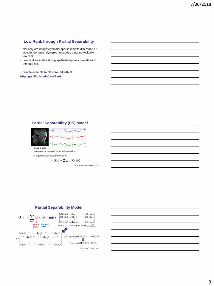
Low Rank through Partial Separability

• Not only are images typically sparse in finite difference or

wavelet domains, dynamic timeseries data are typically

low rank

• Low rank indicates strong spatial-temporal correlations in

the data set.

• Simple example to play around with at:

http://go.illinois.edu/LowRank

Partial Separability (PS) Model

Leverages strong spatiotemporal correlation

Lth order Partial Separability model:

/loo/ - /lee/ - /la/ sounds

100 frames per second

Z.-P. Liang, IEEE-ISBI, 2007.

Partial Separability Model

Z.-P. Liang, IEEE-ISBI, 2007.

7/30/2018

10

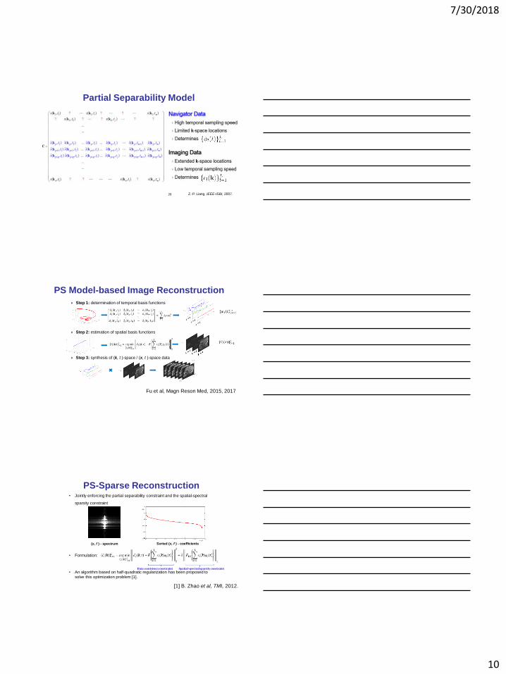
Partial Separability Model

28 Z.-P. Liang, IEEE-ISBI, 2007.

Step 1: determination of temporal basis functions

Step 2: estimation of spatial basis functions

Step 3: synthesis of (k, t )-space / (x, t )-space data

PS Model-based Image Reconstruction

Fu et al, Magn Reson Med, 2015, 2017

PS-Sparse Reconstruction• Jointly enforcing the partial separability constraint and the spatial-spectral

sparsity constraint

• Formulation:

• An algorithm based on half-quadratic regularization has been proposed to solve this optimization problem [1].

dB

× 105

(x, f ) - spectrum

[1] B. Zhao et al, TMI, 2012.

Sorted (x, f ) - coefficients

Data consistency constraint Spatial-spectral sparsity constraint

7/30/2018

11

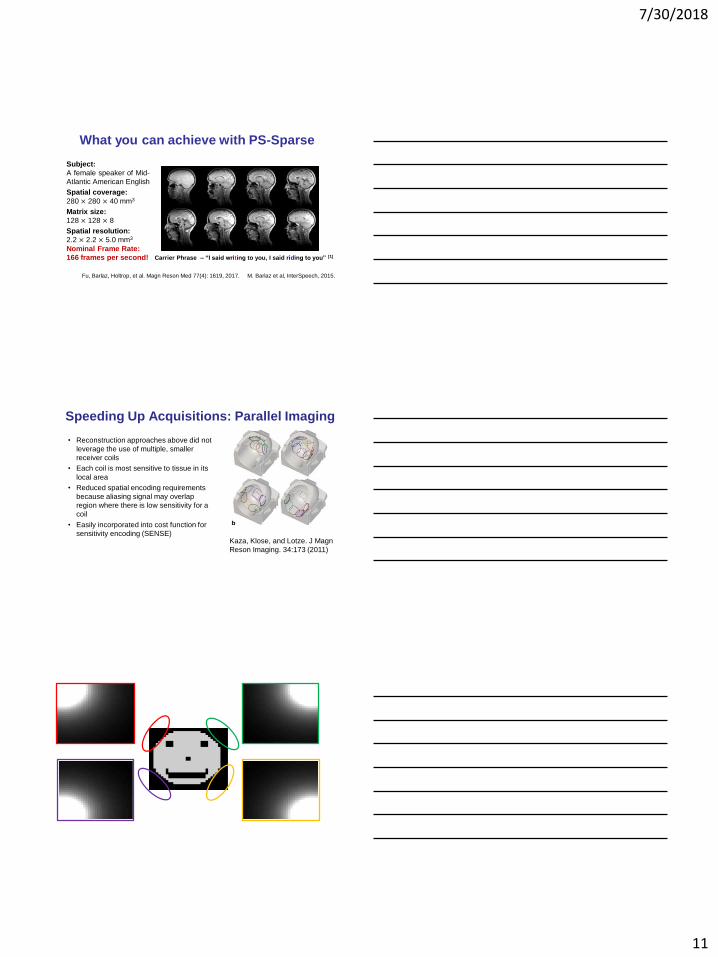
Subject:

A female speaker of Mid-

Atlantic American English

Spatial coverage:

280 × 280 × 40 mm3

Matrix size:

128 × 128 × 8

Spatial resolution:

2.2 × 2.2 × 5.0 mm3

Nominal Frame Rate:

166 frames per second!

What you can achieve with PS-Sparse

Carrier Phrase – “I said writing to you, I said riding to you” [1]

Fu, Barlaz, Holtrop, et al. Magn Reson Med 77(4): 1619, 2017. M. Barlaz et al, InterSpeech, 2015.

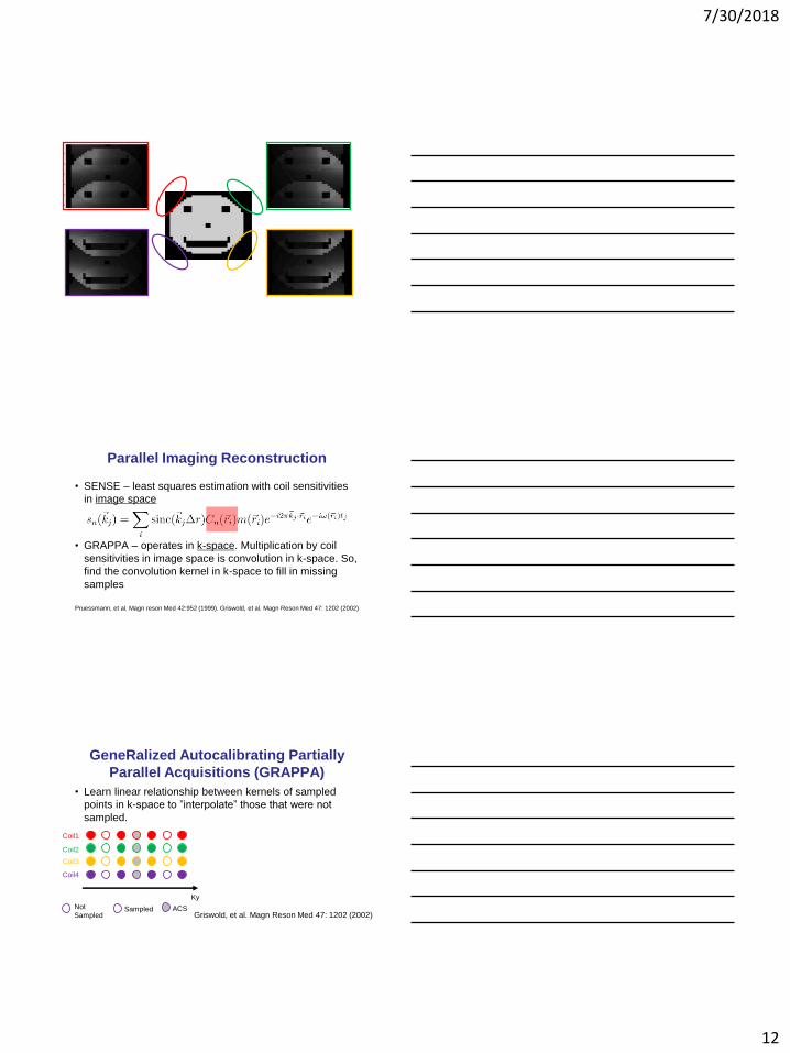
Speeding Up Acquisitions: Parallel Imaging

• Reconstruction approaches above did not

leverage the use of multiple, smaller

receiver coils

• Each coil is most sensitive to tissue in its

local area

• Reduced spatial encoding requirements

because aliasing signal may overlap

region where there is low sensitivity for a

coil

• Easily incorporated into cost function for

sensitivity encoding (SENSE)Kaza, Klose, and Lotze. J Magn

Reson Imaging. 34:173 (2011)

7/30/2018

12

Parallel Imaging Reconstruction

• SENSE – least squares estimation with coil sensitivities

in image space

• GRAPPA – operates in k-space. Multiplication by coil

sensitivities in image space is convolution in k-space. So,

find the convolution kernel in k-space to fill in missing

samples

Pruessmann, et al. Magn reson Med 42:952 (1999). Griswold, et al. Magn Reson Med 47: 1202 (2002)

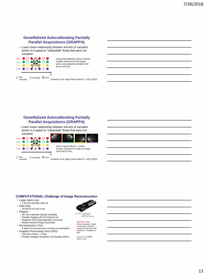
GeneRalized Autocalibrating Partially

Parallel Acquisitions (GRAPPA)

• Learn linear relationship between kernels of sampled

points in k-space to ”interpolate” those that were not

sampled.

Griswold, et al. Magn Reson Med 47: 1202 (2002)

Ky

Coil1

Coil2

Coil3

Coil4

Not

SampledSampled ACS

7/30/2018

13

GeneRalized Autocalibrating Partially

Parallel Acquisitions (GRAPPA)

• Learn linear relationship between kernels of sampled

points in k-space to ”interpolate” those that were not

sampled.

Griswold, et al. Magn Reson Med 47: 1202 (2002)Not

SampledSampled

Ky

Coil1

Coil2

Coil3

Coil4

ACS

Using Autocalibration points, find the

weights required to fit the target

point, using adjacent samples from

across all coils.

GeneRalized Autocalibrating Partially

Parallel Acquisitions (GRAPPA)

• Learn linear relationship between kernels of sampled

points in k-space to ”interpolate” those that were not

sampled.

Griswold, et al. Magn Reson Med 47: 1202 (2002)Not

SampledSampled

Ky

Coil1

Coil2

Coil3

Coil4

ACS

Then Slide the kernel around to fill in

the missing k-space points

Once k-space filled in – simply

Fourier Transform to make an image

from EACH COIL.

COMPUTATIONAL Challenge of Image Reconstruction• Large matrix size

– 1.25 mm isotropic data set

• Data Size: – 18 GB for 6.5 min scan

• Physics: – 3D non-Cartesian (Spiral) sampling

– Parallel Imaging with 32 channel coil

– Magnetic Field Inhomogeneity Correction

– Motion-induced Phase Correction

• Reconstruction Time– 8 days for reconstruction running on workstation

• Graphics Processing Units (GPU) – 200 times faster: <1 hour.

– Enables imaging resolutions not feasible before.

IMPATIENT MRI:

Illinois Massively Parallel

Acceleration Toolkit for

Image reconstruction with

ENhanced Throughput in

MRI

PowerGrid –ISMRM

2016, p. 525

GTX 1080 Ti: ~$700 (11 GB)

CORES: 3584

Boost Clock: 1582 MHz

7/30/2018

14

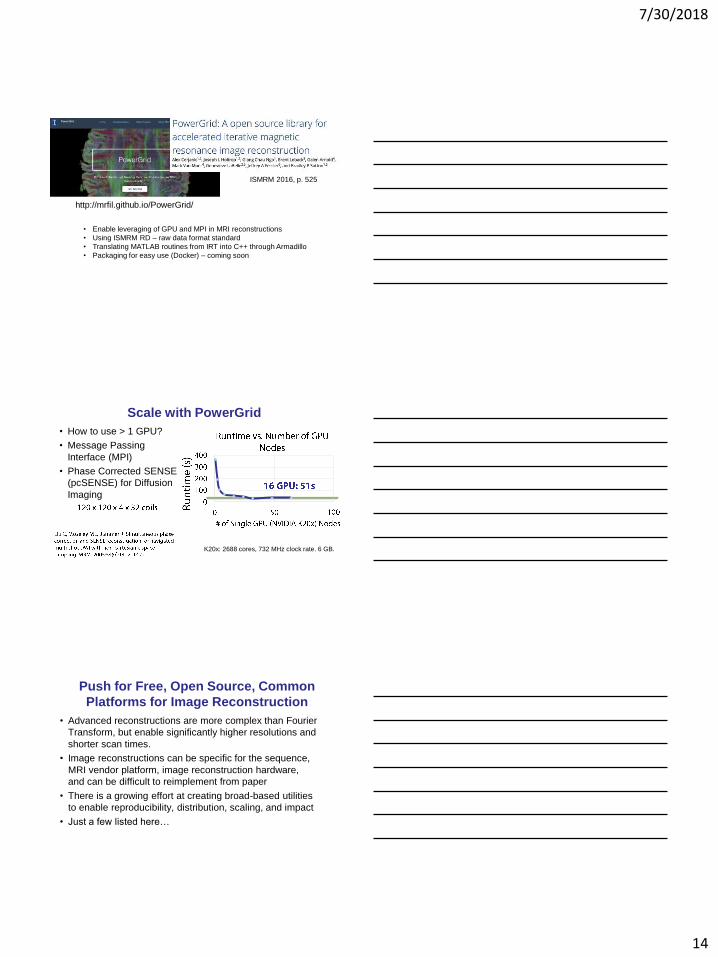
http://mrfil.github.io/PowerGrid/

ISMRM 2016, p. 525

• Enable leveraging of GPU and MPI in MRI reconstructions

• Using ISMRM RD – raw data format standard

• Translating MATLAB routines from IRT into C++ through Armadillo

• Packaging for easy use (Docker) – coming soon

Scale with PowerGrid

• How to use > 1 GPU?

• Message Passing

Interface (MPI)

• Phase Corrected SENSE

(pcSENSE) for Diffusion

Imaging

K20x: 2688 cores, 732 MHz clock rate. 6 GB.

Push for Free, Open Source, Common

Platforms for Image Reconstruction

• Advanced reconstructions are more complex than Fourier

Transform, but enable significantly higher resolutions and

shorter scan times.

• Image reconstructions can be specific for the sequence,

MRI vendor platform, image reconstruction hardware,

and can be difficult to reimplement from paper

• There is a growing effort at creating broad-based utilities

to enable reproducibility, distribution, scaling, and impact

• Just a few listed here…

7/30/2018

15

Hansen and Sorensen. Gadgetron. Magn Reson

Medicine 69: 1768 (2013)

https://www.ismrm.org/MR-Hub/

https://web.eecs.umich.edu/~fessler/code/index.html

Summary

• Inverse problem approach to MRI reconstruction enables

higher resolution, improved SNR, accommodating non-

ideal physics for improved image quality

• Comes at a great deal of computational expense (MRI

scanner does an efficient job for FFT on Cartesian data)

• Lots of open source powerful code available to translate

techniques to clinical research workflows, leveraging

clusters and GPU’s

– TRY THEM OUT!