Slides on �deeper roots�papers

November 29, 2015

Empirical macro/development often about �nding (cross-country) correlations,maybe causation

(Often) not about �nding deeper roots

Example: say we �nd factor X (e.g., democracy) causes development; then whydo some countries have factor X and others not?

More ambitious approach: �nd the deeper (historic) roots that caused factor X

Often requires us to overcome challenges in terms of measuring those deeperfactors:

� Data is poor

� Unit of observation not clear (country?); migration

Still important to try

Bockstette, Chanda, and Putterman (2002)

One of the �rst papers compiling a �deeper roots� variable

Followed by later extensions

Still often cited by others using the data

Idea: create �index of the depth of experience with state-level institutions�(abstract)

Motivation:

� Statehood initially absent everywhere, began developing in certain clustersaround the world

� Poorest regions today often in parts of Sub-Saharan Africa, where statestructures were historically weaker (Mozambique)

� Rapid development since 1960 in regions with large empires in ancienttimes (China)

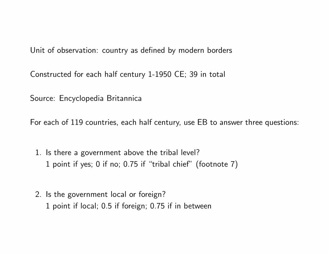
Unit of observation: country as de�ned by modern borders

Constructed for each half century 1-1950 CE; 39 in total

Source: Encyclopedia Britannica

For each of 119 countries, each half century, use EB to answer three questions:

1. Is there a government above the tribal level?1 point if yes; 0 if no; 0.75 if �tribal chief� (footnote 7)

2. Is the government local or foreign?1 point if local; 0.5 if foreign; 0.75 if in between

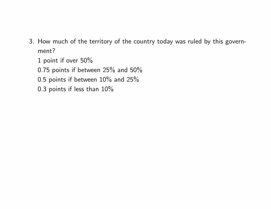
3. How much of the territory of the country today was ruled by this govern-ment?1 point if over 50%0.75 points if between 25% and 50%0.5 points if between 10% and 25%0.3 points if less than 10%

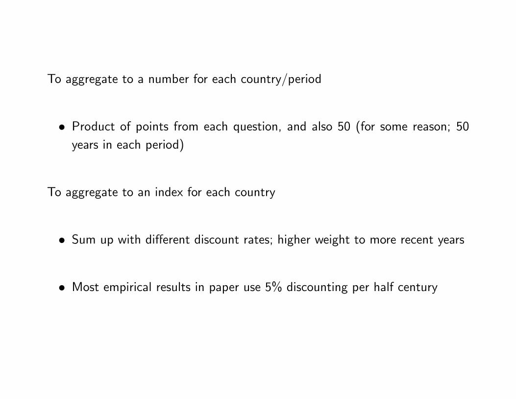
To aggregate to a number for each country/period

� Product of points from each question, and also 50 (for some reason; 50years in each period)

To aggregate to an index for each country

� Sum up with di¤erent discount rates; higher weight to more recent years

� Most empirical results in paper use 5% discounting per half century

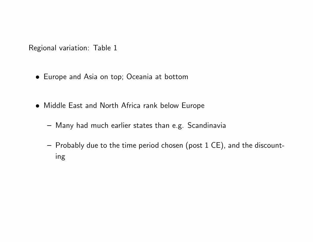
Regional variation: Table 1

� Europe and Asia on top; Oceania at bottom

� Middle East and North Africa rank below Europe

� Many had much earlier states than e.g. Scandinavia

� Probably due to the time period chosen (post 1 CE), and the discount-ing

Cross-country correlations: Table 2

� Note * here means highest level of signi�cance

� Positive, signi�cant correlations with economic growth after 1960, andlevels for later years (but not 1960)

� Also some indications that past state presence is associated with betterstate performance in modern times

Regressions with growth since 1960 as dependent variable

State history has a robust e¤ect on growth in GDP per capita

� Whole world: Table 3

� OECD: Table 4

Levels regressions: weaker results

Seems e¤ects of state history show up mostly after 1960

Paper does not give many detailed on interpretations

� Maybe rise in trade, or other global changes since 1960, bene�ted countrieswith more state history; complementarity?

Borcan, Olsson, and Putterman (2014)

Update of state history data following same methodology as Bockstette et al.(2002)

Now from 3500 BCE to 2000 CE; essentially a complete global measure of statehistory up until now

� 3500 BCE is the rough birth date of the �rst documented state (Uruk inthe Middle East); zero state presence before that

� Global state presence by now, more or less

Other additions compared to Bockstette et al. (2002)

� More detailed explanation of the methodology for constructing the data

� More countries (159)

� Richer descriptive results; use of time/panel structure; lessons about hu-man history beyond economics

� More regression results

� Agriculture)Statehood

� Statehood)Development

On the methodology

zjit 2 [0; 1] = score on question j, for half-century t, country i

Now State index, si;t 2 [0; 50], is a time/country dependent ��ow� variablemeasuring degree of state presence (or statehood) in country i, time t

si;t = 50z1itz2itz3it

(slightly more complicated if there was a change in the scores within a half-century)

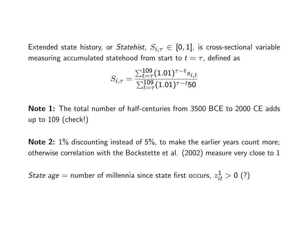
Extended state history, or Statehist, Si;� 2 [0; 1], is cross-sectional variablemeasuring accumulated statehood from start to t = � , de�ned as

Si;� =

P109t=�(1:01)

��tsi;tP109t=�(1:01)

��t50

Note 1: The total number of half-centuries from 3500 BCE to 2000 CE addsup to 109 (check!)

Note 2: 1% discounting instead of 5%, to make the earlier years count more;otherwise correlation with the Bockstette et al. (2002) measure very close to 1

State age = number of millennia since state �rst occurs, z1it > 0 (?)

More variables of interest

Agyears = number of millennia since introduction of agriculture; from separatework by Putterman with Trainor (2006)

Origtime = time (in millennia?) since initial human settlement, from Ahlerupand Olsson (2012); note human settlement came long before agriculture (mostly)

Log GDP per capita in 2000 CE

Geography controls

Absolute latitude, distance to coast/river, elevation, percent arable land, pre-cipitation, temperature, malaria exposure, landlocked

Other

Population density in 1, 1500 CE (originally from McEvedy and Jones 1978)

Urbanization in 1, 1500 CE

Technology adoption in 1, 1500, 2000 CE

Descriptive results: Figures 1, 2

Periods of spurts, stagnation, in the world average

Western region mostly highest scores; here includes North Africa, Middle East,Europe

Americas and SSA have lower scores; spurt at the end

Some reversals toward the end, due to colonization (recall how index gave lowerscores if foreign government); cf. Fig C1 in appendix

Regressions

First link: agriculture (+other stu¤))statehood

Agriculture came before statehood for (almost) all countries; cf. Figure B1

Causation (most likely) from former to latter

Statei = �0 + �1 � Agyearsi + controlsi + �i

State represents either accumulated index in 2000 (Si;2000) or Stateage (seeabove)

Tables 2, 3

� Strong, robust, positive correlation between time since agriculture andamount of, or time since, statehood

� Well known; �rst states where agriculture began (Fertile Crescent)

� Table 2, column (1): one more millennium since introduction of agriculture=) 0:47 more millennia (470 years) since �rst state

� None or small e¤ect from Origtime, once controlling for agriculture: rootsnot that deep

� Table 3: di¤erentiating between how �rst state established: internally orexternally; latter means ruled by other government

� Stronger e¤ect of Agyears for internally established states (interpretation?)

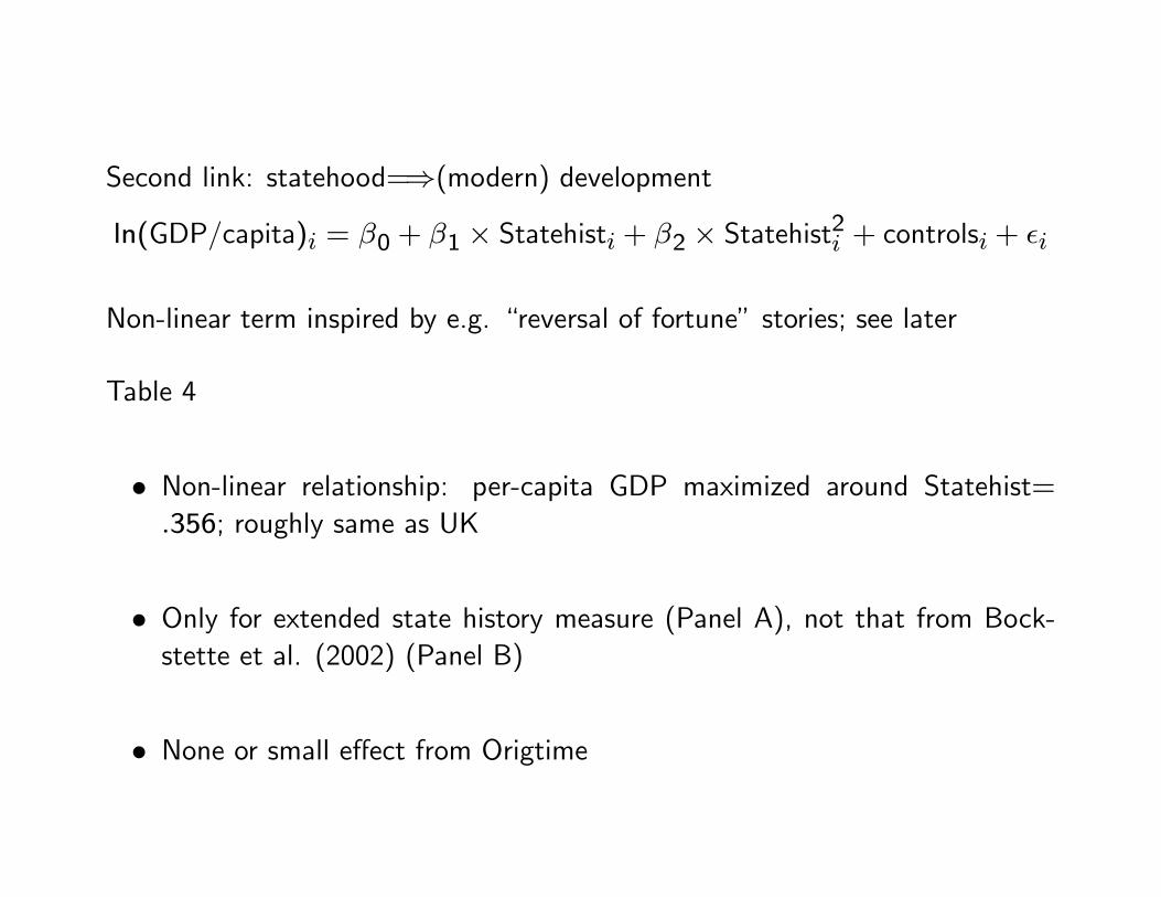
Second link: statehood=)(modern) development

ln(GDP/capita)i = �0 + �1 � Statehisti + �2 � Statehist2i + controlsi + �i

Non-linear term inspired by e.g. �reversal of fortune� stories; see later

Table 4

� Non-linear relationship: per-capita GDP maximized around Statehist=:356; roughly same as UK

� Only for extended state history measure (Panel A), not that from Bock-stette et al. (2002) (Panel B)

� None or small e¤ect from Origtime

Table 5

� Acenstry-adjusted measures, using Putterman-Weil matrix (more later)

� Idea: let e.g. Canada�s state history be a weighted average of those ofpeoples migrating there after 1500

� Use both state history up to 1500 (Panel A), and up to 2000 (Panel B)

� Non-linear relationship even stronger, but not so robust for the 2000 mea-sure (why?)

Tables 6, 7, 8: skip for now

Acemoglu, Johnson, and Robinson (2002)

Older paper again, with big impact at the time

One in a series of papers by same authors on institutions and development; seee.g. 2001 AER paper on settler mortality

Idea: countries/societies that were more developed around 1500 are poor todaybecause of European colonization

� Higher levels of development in 1500 meant better infrastructure for ex-traction, and more to extract

� This induced Europeans to set up extractive institutions, which led tounderdevelopment later

� Other locations became Neo-Europes, meaning Europeans migrated there,and set up (European) institutions that allowed private property, oftenlabelled inclusive institutions in later work

� (Premise here that European institutions already were relatively inclusiveby 1500)

Examples: Extractive institutions in Latin America; non-extractive ones inNorth America

Phenomenon labelled Reversal of Fortune

Some further observations when reading introduction through the lens of morerecent research:

� Main motivation in terms of institutions or geography; dichotomy empha-sized but not motivated much

� No discussion about whether geography could a¤ect Europe�s institutions,or early development elsewhere (strange reading of Jared Diamond inNippe�s opinion)

� But we know that either geography, or chance, must be the fundamentaldeterminant of institutions. This does not shine through anywhere in thetext

� Later work by A+R (e.g.,�Why Nations Fail�) uses concepts like insti-tutional drift; probably what they had in mind in their 2002 QJE papertoo

Data:

� Log GDP/capita in modern times

� Proxies for past development:

� Urbanization around 1500 from Bairoch and other sources

� Population density around 1500 from McEvedy and Jones (1978)

� Big issue if these proxy for GDP/capita or something else; think ofstandard Malthusian model

� Institutions:

� Protection again expropriation risk 1985-95 from Political Risk Services

� Constraints on the Executive in 1990; variable from Polity III data(earlier version of the same dataset used to measure democracy)

� Same as above but for �rst year of independence (Polity data onlyde�ned for independent countries)

� Only last measure is non-contemporary

� Instrument for institutional choices: settler mortality

� Geography controls etc.

Table III: urbanization in 1500)modern development

� Sample: former colonies

� Negative and signi�cant e¤ects: more urban (=richer?) countries in 1500are poorer today

� Robust to changes in the sample composition

� Table IV: varying how urbanization is measured

Table V: population density in 1500)modern development

� Similar results as for urbanization

� Note e.g. results with arable land and population entered separately (PanelB); seems density is what matters

Table VI: more robustness checks

� Note columns (9), (10): urbanization does not have negative e¤ect insample of non-colonies, suggesting the pattern should be explained bycolonization

� (But how about population density?)

Section III.D of the paper

� E¤ect had nothing to do with Europeans simply stealing resources; nochange immediately after 1500

� Per-capita income di¤erences emerge later; Figures IVa-b

So far documenting that there was some sort of reversal. But why?

AJR�s preferred explanation: institutions

What determined the type of institutions colonial powers set up?

1. What seemed pro�table. In places with high population density you canenslave and/or tax the population

2. Whether Europeans could settle. In colder places (e.g. Canada) Europeansdid not die from tropical diseases

Guides their choice of IV variables

Table VII: urbanization, population density in 1500)institutions

� Dependent variable: institutions measured by one of the three variablesabove

� Two contemporary; one measured at independence

� Both independent variables (urbanization, population density in 1500) sig-ni�cant with the right sign

� Although not so much when entered together? (cf. Footnote 21)

Table VIII: IV regressions

� Y = log GDP/capita in 1995

� X = institutions

� Z = settler mortality

� (urbanization, population density in 1500 enter �rst and second stage aswell)

� AJR argue their institutions story consistent with the results in Table VIII

Valid speci�cation?

� Only if settler mortality (Z) a¤ected modern development (Y) throughinstitutions (X) only and not directly

� Controversial topic still today

� Je¤rey Sachs and others believe, e.g., malaria hampers development

� Other aspects of the settler mortality instrument also controversial

� See Albouy (AER 2012); replies by AJR

Yet another angle on the reversal-of-fortune theory

� In terms of the population, the Neo-Europes were more or less copies ofthe powers that colonized them

� Example: US and Canada have mostly English (+French) language,traditions, institutions, cultures, etc.

� But all regressions use urbanization, population density in pre-colonizedNorth America

� Alternative approach: use ancestry-adjusted measures (Putterman andWeil 2010, Chanda et al 2014)

Putterman and Weil (2010)

Ambition: create a matrix that gives a complete description of migration since1500; source and target countries

Q. Consider the population of country i in 2000. What fraction of this popu-lation had its ancestors in 1500 living in country j?

Very di¢ cult question to answer

Main source: genetic data on di¤erences in allele frequencies; allele is a se-quence at a particular position in the DNA; see Appendix I for details onprinted/online sources (e.g. CIA World Factbook)

Many problems/issues. Examples:

� How do you assign source country to people with mixed ancestry? Answer:treat them as having fractions of their ancestry in di¤erent source countries,e.g., 40% Swedish, 60% Chinese

� If someone�s ancestors lived in country A in 1500, and country B in 1800,which counts as source country? Answer: country A

Suppose we have an answer to question Q above for each country pair i and j

This generates a matrix

� 165 rows, one for each present-day country

� 172 columns, one for each possible source country (same 165 plus 7 moresmall countries)

� All elements between 0 and 1; most close to one along the diagonal

� Rows sum to one

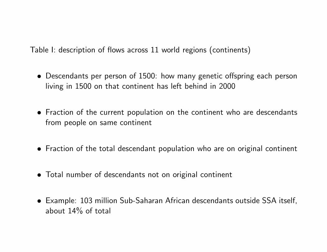
Table I: description of �ows across 11 world regions (continents)

� Descendants per person of 1500: how many genetic o¤spring each personliving in 1500 on that continent has left behind in 2000

� Fraction of the current population on the continent who are descendantsfrom people on same continent

� Fraction of the total descendant population who are on original continent

� Total number of descendants not on original continent

� Example: 103 million Sub-Saharan African descendants outside SSA itself,about 14% of total

Next step: use matrix to ancestry adjust some early-development variables

� State history from Bockstette et al.; here denoted statehist

� 5% discounting, 1-1500 CE (29 half centuries)

� Millennia since Neolithic; here denoted agyears

Example

Two countries, A and B, with statehist levels .9 and .1, respectively

80% of people in A have ancestors in A, rest have ancestors in B

90% of people in B have ancestors in A, rest have ancestors in B

":74:82

#| {z }

adjusted statehist

=

":72 + :02:81 + :01

#=

":8 :2:9 :1

#| {z }PW-matrix

�":9:1

#| {z }

statehist

Which countries�statehist, agyears change when ancestry adjusted? Figures II,III

Main results: Table II

� Bigger coe¢ cient estimates, more precise estimates, higher R2 with ad-justed than non-adjusted measures

Alternative ways to adjust: Table III

� Assigning statehist, agyears of UK to all Neo-Europes: columns (1)-(4)

� Fraction native, fraction retained as controls: (5)-(6)

� Fraction European descent, fraction European languages as controls: (7)-(12)

Tables IV: add geography controls

� Variables

� Landlocked dummy

� Eurasia dummy

� Absolute latitude

� Suitability for agriculture; 4-point measure from Hibbs and Olsson(PNAS 2004)

� Ancestry-adjusted statehist, agyears still signi�cant

Table V: other measures of early development than statehist, agyears

� First two meant to capture mechanisms related to Diamond (1997)

� geo conditions: �rst principle component of �climate�, latitude, sizeof landmass, east-west orientation of land mass; based on Olsson andHibbs (EER 2005)

� bio conditions: �rst principle component of: number of domsticableanimals, wild plants suitable for creating agricultural seeds

� Technology measures from Comin et al. (2010)

� Believed to have impacted timing of transition to agriculture, statehoodaccording to Jared Diamond

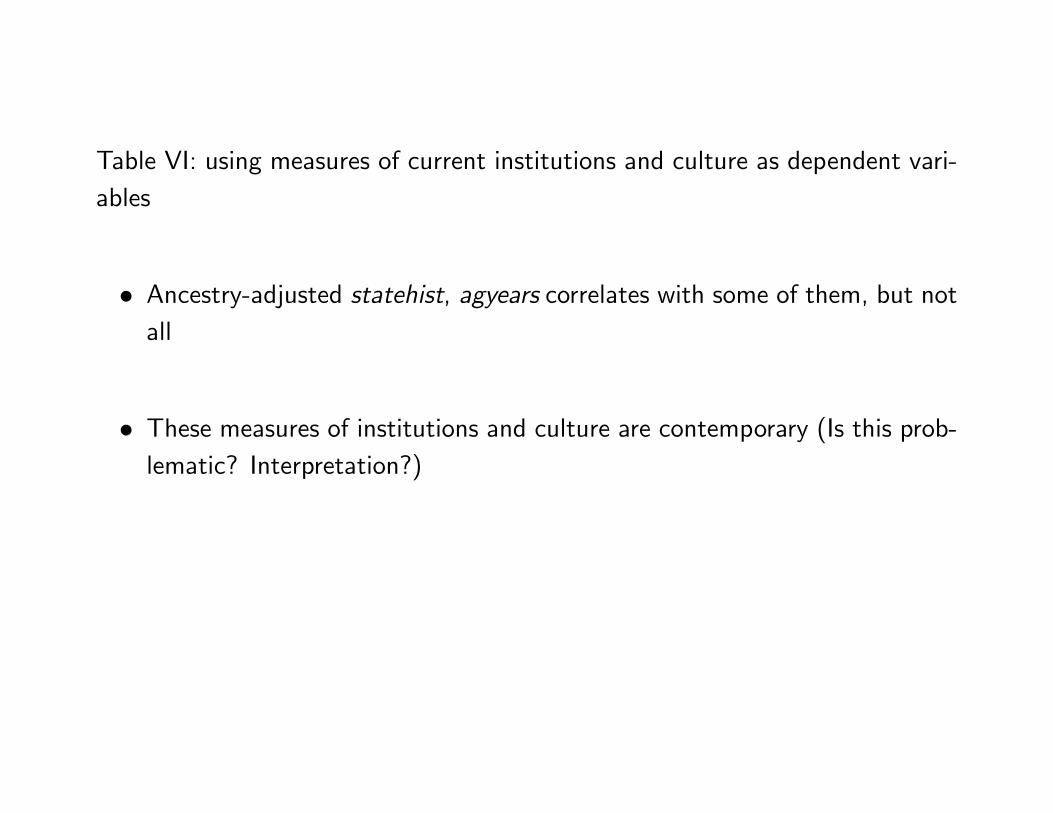
Table VI: using measures of current institutions and culture as dependent vari-ables

� Ancestry-adjusted statehist, agyears correlates with some of them, but notall

� These measures of institutions and culture are contemporary (Is this prob-lematic? Interpretation?)

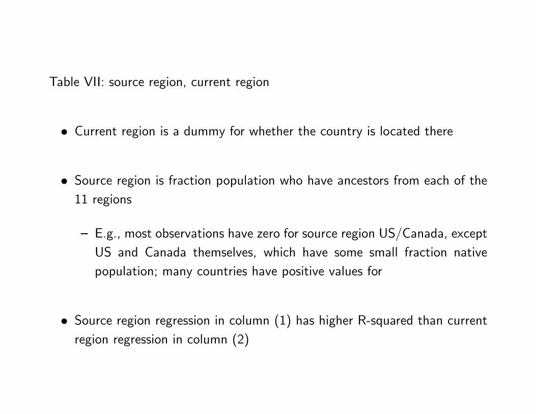
Table VII: source region, current region

� Current region is a dummy for whether the country is located there

� Source region is fraction population who have ancestors from each of the11 regions

� E.g., most observations have zero for source region US/Canada, exceptUS and Canada themselves, which have some small fraction nativepopulation; many countries have positive values for

� Source region regression in column (1) has higher R-squared than currentregion regression in column (2)

� Column (3): both sets of variables together; being from Europe by ancestryis better than being there now, same for East Asia

Table VIII: heterogeneity in early development

� Weighted within-country standard deviation in ancestral statehist, agyearsfor each group; weights are those used for ancestry adjustment

� Standard deviation has positive e¤ect; heterogeneity in the population�sancestry-adjusted early development is �good�

Tables IX-XI: skip for now

Chanda, Cook, and Putterman (2010)

New look at Acemoglu, Johnson and Robinson (2002)

Benchmark: same focus on colonized countries, same outcome variable (logGDP/capita in 1995), as AJR

Two robustness checks:

� Ancestry adjustment of AJR�s measures of preindustrial development: pop-ulation density and urbanization around 1500

� Add new variables measuring early development: time since agriculture,state history, technology in 1500 (last one from Comin, Easterly, and Gong2010)

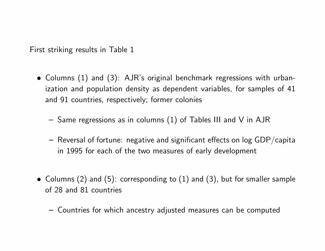
First striking results in Table 1

� Columns (1) and (3): AJR�s original benchmark regressions with urban-ization and population density as dependent variables, for samples of 41and 91 countries, respectively; former colonies

� Same regressions as in columns (1) of Tables III and V in AJR

� Reversal of fortune: negative and signi�cant e¤ects on log GDP/capitain 1995 for each of the two measures of early development

� Columns (2) and (5): corresponding to (1) and (3), but for smaller sampleof 28 and 81 countries

� Countries for which ancestry adjusted measures can be computed

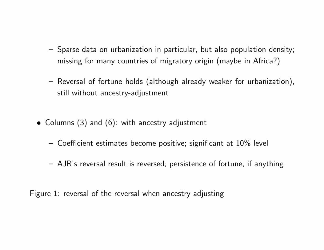
� Sparse data on urbanization in particular, but also population density;missing for many countries of migratory origin (maybe in Africa?)

� Reversal of fortune holds (although already weaker for urbanization),still without ancestry-adjustment

� Columns (3) and (6): with ancestry adjustment

� Coe¢ cient estimates become positive; signi�cant at 10% level

� AJR�s reversal result is reversed; persistence of fortune, if anything

Figure 1: reversal of the reversal when ancestry adjusting

Next : introduce the new measures

Table 2: all �ve (two old, three new) show positive pairwise correlations (as wealready knew for some of them)

� Seem to broadly measure similar dimension of preindustrial development

� Note, however, the low correlation between urbanization and both timesince agriculture and technology in 1500; small samples

Table 3: regression with the three new variables, ancestry adjusted and not

� Negative signs, but insigni�cant, with no adjusting: AJR�s result not robusteven without ancestry-adjustment

� Signs positive and now also highly signi�cant when ancestry adjusting

� See Figure 2 for illustration

Robustness checks of the robustness checks

Table 4: add same controls as in AJR Tables III and V, columns (8)-(11):labelled latitude, climate, resources, and religion

Results in Tables 1 and 3 do not change

� For urbanization and population density: ancestry adjusting makes previ-ously negative and signi�cant e¤ects become positive, mostly insigni�cant;(more) signi�cant when controlling for religion

� Recall small sample of 28 and 41 countries respectively

� For remaining three: results go from insigni�cant, with varying signs, tonegative and mostly signi�cant (never below 10%)

� Larger samples

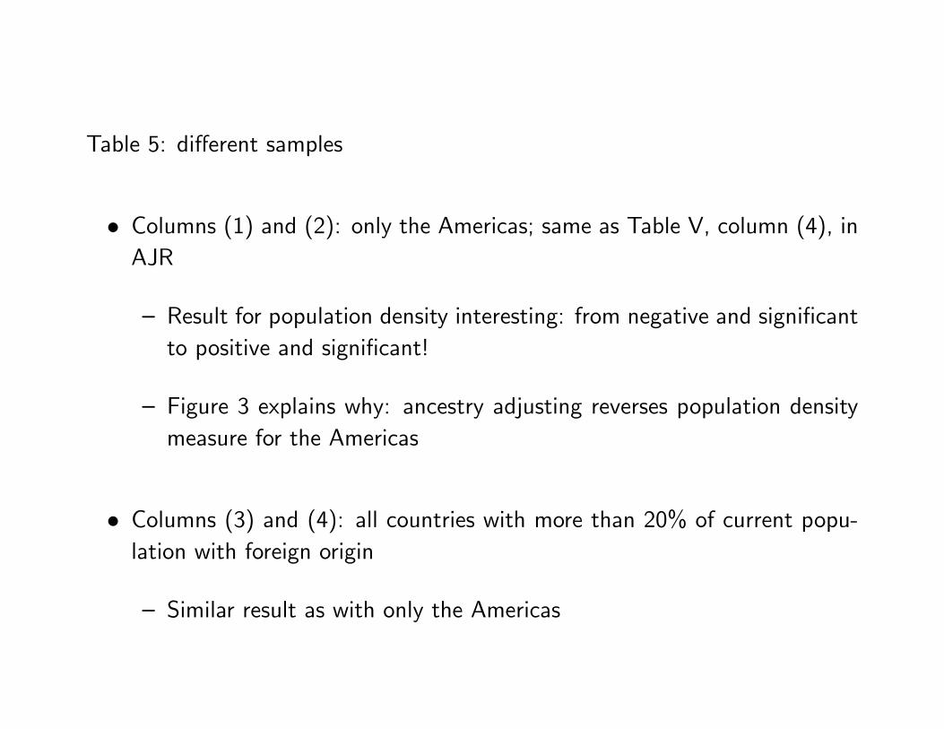
Table 5: di¤erent samples

� Columns (1) and (2): only the Americas; same as Table V, column (4), inAJR

� Result for population density interesting: from negative and signi�cantto positive and signi�cant!

� Figure 3 explains why: ancestry adjusting reverses population densitymeasure for the Americas

� Columns (3) and (4): all countries with more than 20% of current popu-lation with foreign origin

� Similar result as with only the Americas

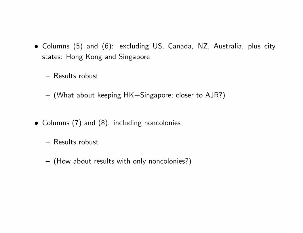
� Columns (5) and (6): excluding US, Canada, NZ, Australia, plus citystates: Hong Kong and Singapore

� Results robust

� (What about keeping HK+Singapore; closer to AJR?)

� Columns (7) and (8): including noncolonies

� Results robust

� (How about results with only noncolonies?)

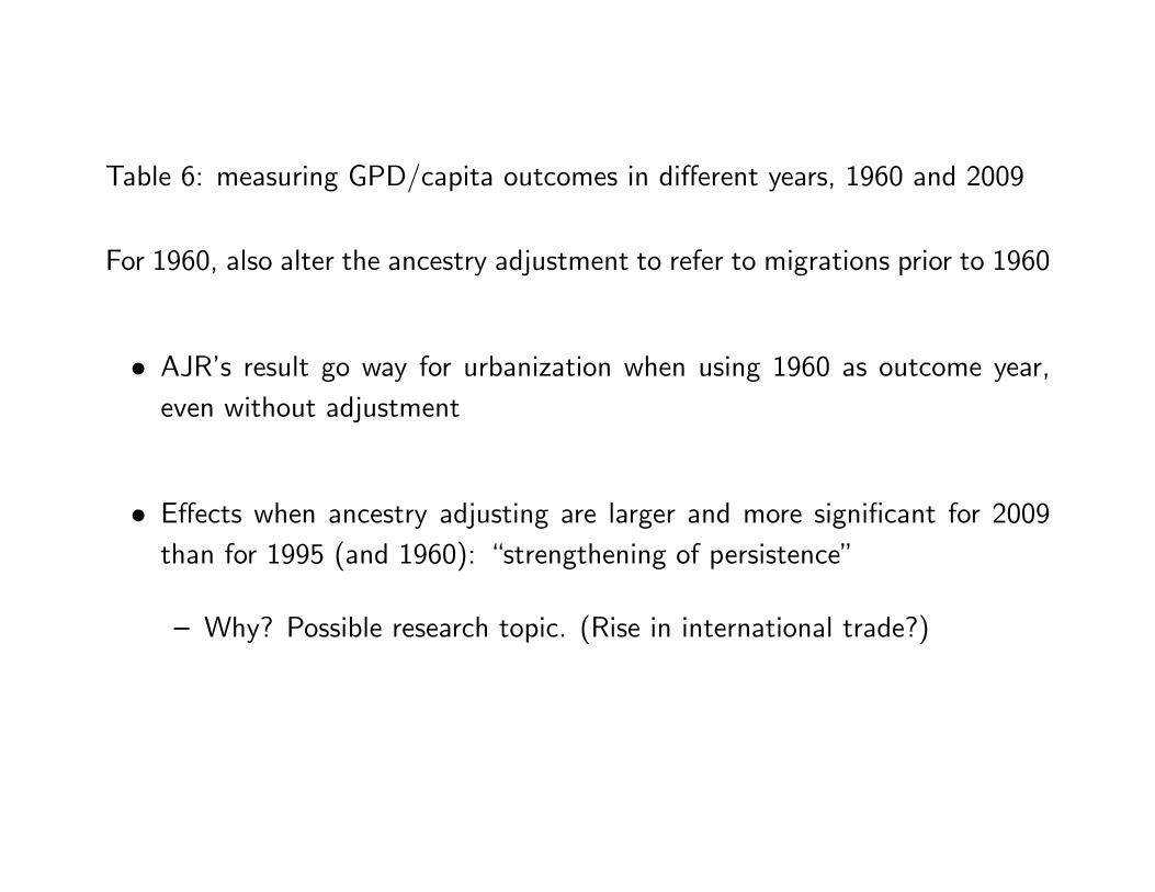
Table 6: measuring GPD/capita outcomes in di¤erent years, 1960 and 2009

For 1960, also alter the ancestry adjustment to refer to migrations prior to 1960

� AJR�s result go way for urbanization when using 1960 as outcome year,even without adjustment

� E¤ects when ancestry adjusting are larger and more signi�cant for 2009than for 1995 (and 1960): �strengthening of persistence�

� Why? Possible research topic. (Rise in international trade?)

Section III of paper (on channels) � skip for now

Hariri (2012)

Examines link state history)democracy

Story all about colonial histories

Related to AJR (2002), but outcome variable democracy rather than log GPD/capita

Natural starting point for many political scientists; paper in the American Po-litical Science Review (APSR)

Story

How strong state a country had at the onset of the colonial period (around1500) determined its colonial experience: whether of was colonized at all, and,if it was, how much, and what type of colonization

� Some countries had strong enough states to resist European coloniza-tion altogether; this also enabled them to suppress local opposition)lessdemocracy today

� Examples: Ethiopia (only African country not to be colonized); China;Japan

� Others were conquered and then ruled by European powers through exist-ing state infrastructure (extractive institutions in AJR�s terminology))lessdemocracy today

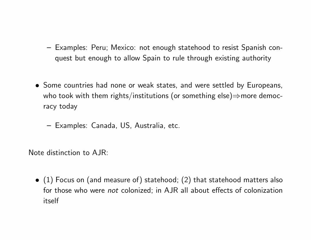
� Examples: Peru; Mexico: not enough statehood to resist Spanish con-quest but enough to allow Spain to rule through existing authority

� Some countries had none or weak states, and were settled by Europeans,who took with them rights/institutions (or something else))more democ-racy today

� Examples: Canada, US, Australia, etc.

Note distinction to AJR:

� (1) Focus on (and measure of) statehood; (2) that statehood matters alsofor those who were not colonized; in AJR all about e¤ects of colonizationitself

Econometric speci�cations

Dependent variables:

� Democracy; mainly from Polity IV and referring to period 1991-2007

� Measures of colonization

� Colonial dummy; colonial duration (in centuries)

� Fraction of population speaking European language, or of Europeandescent

� Extent of indirect rule (fraction colonially recognized court cases; seepaper)

Independent variables:

� State history up to 1500, from Putterman�s website (Bockstette et al.2002)

Instrument:

� Time since agriculture

Results

Table 1, Figure 1: State history)democracy

� More state history, less democracy

Table 2, Figure 2: instrumenting statehood with time since agriculture

� Results from Table 1 hold

Table 3: State history)colonization

� More state history, less colonization

Table 4: Colonization)democracy

� More colonization, more democracy