slovak university of technology in bratislava faculty of
TRANSCRIPT
2017 Bc. Martin Mišenko
SLOVAK UNIVERSITY OF TECHNOLOGY IN
BRATISLAVA
FACULTY OF CHEMICAL AND FOOD TECHNOLOGY
REG. NO.: FCHPT-5414-61616
STABILISATION OF COLUMN FEED USING APC
MASTER THESIS


Bratislava 2017 Bc. Martin Mišenko
SLOVAK UNIVERSITY OF TECHNOLOGY IN
BRATISLAVA
FACULTY OF CHEMICAL AND FOOD TECHNOLOGY
Reg. No.: FCHPT-5414-61616
STABILISATION OF COLUMN FEED USING APC
MASTER THESIS
Study program: Automation and Information Engineering in Chemistry and Food Industry
Study field: 5.2.14. Automation
Workplace: Faculty of Chemical and Food Technology
Thesis supervisor: prof. Ing. Miroslav Fikar, DrSc.
Consultant: Ing. Karol Ľubušký


Acknowledgement
I would like to express deep gratitude to my supervisor prof. Ing. Miroslav Fikar, DrSc. for his
guidance and support throughout the master thesis. I also would like to thank refinery Slovnaft
represented by my consultant Ing. Karol Ľubušký for his unwavering support, collegiality and
mentorship throughout this thesis.


Abstract
Liquid tanks are quite common devices in refinery industry. A cascade control is ordinarily used
to control the level in tanks, however, it controls only separate tank and it does not take
interactions between tanks into account. When it is necessary to coordinate control between
tanks, Advanced Process Control (APC) is suitable to implement. APC is multivariable control,
so it can treat the whole system of tanks as one complex system. The aim was to propose and
implement APC control for tanks system at BCDU6 unit in Slovnaft Plc, to mitigate fluctuations
in output flow from the system.
The first part of this work deals with mathematical modeling and basic control of the given tanks
system in Matlab-Simulink. In the second part, we are implementing the APC controller, which
controls the given tank system in BCDU6 unit. We use Honeywell software Profit Suite in this
step.
Key words: Honeywell; APC controller; liquid tanks

Abstrakt
Zásobníky kvapaliny sú bežnou súčasťou rafinérskych zariadení. Na riadenie výšky hladiny sa
zvyčajne používa kaskádová regulácia, ktorá však riadi iba jeden konkrétny zásobník a neberie
do úvahy interakcie s ostatnými zásobníkmi. Ak chceme koordinovať riadenie medzi viacerými
zásobníkmi, je vhodné použiť Advanced Process Control (APC) riadenie. APC je viacrozmerové
riadenie, takže nám umožňuje riadiť systém zásobníkov ako jeden celok. Cieľom práce bolo
navrhnúť a implementovať APC riadenie pre systém zásobníkov na prevádzke AVD6 v Slovnaft
a.s., ktoré bude čím viac tlmiť výkyvy na výstupnom prietoku z riadeného systému.
Práca sa v prvej časti zaoberá matematickým modelovaním a základným riadením zásobníkov
v Matlabe - Simulinku. V druhej časti implementujeme a vyhodnotíme APC regulátor, ktorým
riadime sústavu troch zásobníkov na prevádzke AVD6. Používame pritom software Profit Suite
od spoločnosti Honeywell.
Kľúčové slová: Honeywell; APC regulátor; zásobníky kvapaliny

Table of Contents
Illustrations ........................................................................................................................... 13
Abbreviations ........................................................................................................................ 16
Introduction ........................................................................................................................... 17
1 Bratislava Crude Distillation Unit 6 .............................................................................. 18
1.1 Automatic Control ................................................................................................ 19
1.2 C4 Feed Control .................................................................................................... 21
2 Modeling of the Tank System ........................................................................................ 23
2.1 Derivation of Model .............................................................................................. 24
2.2 Designed Model Validation .................................................................................. 27
3 Slovnaft Control System ................................................................................................ 30
4 Level Control ................................................................................................................. 33
4.1 Parameters for Controller Design ......................................................................... 33
4.2 Averaging Level Control ...................................................................................... 34
4.3 Averaging Control with Gain Scheduling ............................................................. 37
5 Percentage of Working Volume Control ....................................................................... 39
6 Advanced Process Control - RMPCT ............................................................................ 44
6.1 Controller Variables .............................................................................................. 44
6.2 Models .................................................................................................................. 45
6.3 Objective Function ................................................................................................ 45
7 Identification and Controller Design ............................................................................. 46
7.1 Data Preparation ................................................................................................... 46
7.2 Identification ......................................................................................................... 48
7.3 Building Controller ............................................................................................... 55
7.4 Controller Calculations ......................................................................................... 60
8 Controller Configuration ............................................................................................... 66

Discussion ............................................................................................................................. 68
Conclusion ............................................................................................................................ 73
Resumé .................................................................................................................................. 74
Bibliography ......................................................................................................................... 76

13
Illustrations
Fig. 1. Feedback control loop. ............................................................................................... 19
Fig. 2. Cascade control of distillation column. ...................................................................... 20
Fig. 3. C4 feed control .......................................................................................................... 21
Fig. 4. Fluctuation of feed and temperature. ......................................................................... 22
Fig. 5. Tank scheme. ............................................................................................................. 23
Fig. 6. Nonlinear behavior of level indication. ...................................................................... 25
Fig. 7. Volumes to calculate. ................................................................................................. 26
Fig. 8. Linear behavior of percentage of working volume. ................................................... 27
Fig. 9. Input and output flow comparison. ............................................................................ 28
Fig. 10. Input and output flow comparison after correction. ................................................. 29
Fig. 11. Model and Slovnaft level comparison. .................................................................... 29
Fig. 12. Cascade control in Slovnaft ..................................................................................... 30
Fig. 13. Gain scheduling. ...................................................................................................... 31
Fig. 14. Model and Slovnaft PID control performance. ........................................................ 32
Fig. 15. Detail of control performance. ................................................................................. 32
Fig. 16. Parameters for controller design. ............................................................................. 33
Fig. 17. Proportional control only. ........................................................................................ 35
Fig. 18. Averaging level control............................................................................................ 35
Fig. 19. Averaging control with real data. ............................................................................. 36
Fig. 20. Averaging level control with gain scheduling performance. ................................... 37
Fig. 21. Detail of control performance. ................................................................................. 38
Fig. 22. The performance of percentage of working volume control – Slovnaft. ................. 39
Fig. 23. Detail of control performance. ................................................................................. 40
Fig. 24. The performance of percentage of working volume control – averaging control. ... 41
Fig. 25. Detail of control performance. ................................................................................. 41
Fig. 26. Percentage of working volume. ............................................................................... 42
Fig. 27. Reference curve. ...................................................................................................... 43
Fig. 28. Classification of variables for APC. ........................................................................ 46
Fig. 29. Step responses. ......................................................................................................... 47
Fig. 30. Data preparation for PDS. ........................................................................................ 48
Fig. 31. Creating a new model. ............................................................................................. 48
Fig. 32. Data imported in PDS. ............................................................................................. 49

14
Fig. 33. Trials. ....................................................................................................................... 50
Fig. 34. Overall parameters. .................................................................................................. 51
Fig. 35. Fit FIR/PEM/CLid Models. ..................................................................................... 52
Fig. 36. Fitted FIR. ................................................................................................................ 52
Fig. 37. Editing sub-processes. ............................................................................................. 53
Fig. 38. Final trials. ............................................................................................................... 53
Fig. 39. CVs predictions........................................................................................................ 54
Fig. 40. Generating setting files. ........................................................................................... 55
Fig. 41. Error window. .......................................................................................................... 56
Fig. 42. Create a New Application. ....................................................................................... 56
Fig. 43. General information. ................................................................................................ 57
Fig. 44. Controller. ................................................................................................................ 58
Fig. 45. Points. ...................................................................................................................... 58
Fig. 46. Details. ..................................................................................................................... 59
Fig. 47. Connections for Base Level Controls. ..................................................................... 60
Fig. 48. URT Explorer. ......................................................................................................... 61
Fig. 49. New item. ................................................................................................................. 61
Fig. 50. Combinations block. ................................................................................................ 62
Fig. 51. T1 level calculation block. ....................................................................................... 63
Fig. 52. Variable names. ....................................................................................................... 63
Fig. 53. Variable values. ....................................................................................................... 63
Fig. 54. Variable connection. ................................................................................................ 64
Fig. 55. Equation. .................................................................................................................. 65
Fig. 56. CV Summary. .......................................................................................................... 66
Fig. 57. CV Optimize. ........................................................................................................... 66
Fig. 58. MV Summary. ......................................................................................................... 67
Fig. 59. MV Optimize. .......................................................................................................... 67
Fig. 60. DV Summary. .......................................................................................................... 67
Fig. 61. Levels in tanks. ........................................................................................................ 68
Fig. 62. Detail of control performance. ................................................................................. 69
Fig. 63. T1 control. ................................................................................................................ 69
Fig. 64. T2 control. ................................................................................................................ 70
Fig. 65. T3 control. ................................................................................................................ 70
Fig. 66. Final results. ............................................................................................................. 71

15
Fig. 67. Temperature in C1 column. ..................................................................................... 71
Fig. 68. Uniformance PHD trend. ......................................................................................... 72

16
Abbreviations
BCDU6 Bratislava Crude Distillation Unit 6
PID Proportional Integral Derivative Controller
SP Setpoint
K Controller gain
Ts Time constant
Ti Integral time constant
DCS Distributed Control System
FI Flow Indication
LC Level Control
FC Flow Control
LHA Level High Alarm
LLA Level Low Alarm
APC Advanced Process Control
RMPCT Robust Multivariable Predictive Control Technology
CV Controlled Variable
MV Manipulated Variable
DV Disturbance Variable
PV Process Variable
SISO Single Input Single Output
PDS Profit Design Studio
FIR Finite Impulse Response
URT Unified Real Time
PSRS Profit Suite Runtime Studio

17
Introduction
Liquid tanks are common devices used in all chemical industry. We focus on petrochemical
industry, specifically on Bratislava refinery Slovnaft Plc. There is a production unit called
Bratislava Crude Distillation Unit 6 (BCDU6). BCDU6 contains atmospheric and vacuum
distillation parts. Among the vessels in atmospheric part, there are three horizontal cylindrical
tanks (T1, T2, T3), which are subject of our work. Outputs from tanks T1 and T2 are routed into
T3, which is a feed buffer for a redistillation column. Unfortunately, output flows fromT1 and T2
fluctuate, especially the second one. This fact causes fluctuation of T3 feed flow to
the redistillation column. This disturbs heavily operation in the column. Our aim is to decrease
the feed fluctuation as possible.
The first part of this work deals with the synthesis of a mathematical model of treated
tanks, which is necessary for controller design. We have three horizontal cylindrical tanks with
same construction but different parameters. This part also provides verification of derived model
in MATLAB – Simulink. There were designed several types of control systems including
averaging level control, the percentage of working volume control and controller with gain
scheduling. We also reproduced Slovnaft cascade control.
The second part is about APC controller design. At first, we need to define variables and
design model matrix of our sub – processes. Data for identification were prepared in MATLAB
and then exported to Profit Design Studio. After identification, we started with controller
implementation in Profit Suite Runtime Studio. Instead of raw level control, we used a percentage
of working volume for control. Designed controller has been switched on in Slovnaft and some
another improvement were done.

18
1 Bratislava Crude Distillation Unit 6
The first step in crude processing in an oil refinery is distillation. Distillation separates crude oil
to several fractions. It is physical process based on different boiling temperatures of desired
fractions. It means that hydrocarbons already present in crude are separated and no chemical
changes are intended. Its products do not satisfy requirements for final products and various
refinery units treat them. Slovnaft refinery has two crude oil distillation units – BADU5 and
BCDU6. Since our work is oriented on BCDU6, we will deal only with this one in following parts
of work.
Technology Description
Since BCDU6 technology is quite complex, we will focus only on control systems and its
upstream processes. The first step in crude distillation is desalination. Oil is preheated in a heat
exchange system and mixed with wash water. Water is added to dissolve the salts and clear out
mechanical impurities. A mixture of oil and water enters desalter tanks, where hydrocarbons and
water are separated.
Desalted crude oil is preheated and enters preflash column. The main task of preflash
column is to separate the lightest hydrocarbon fractions from oil and thus unload atmospheric
furnace and column. C1 overhead product is called preflash heavy naphtha. Bottom product of C1
is called preflash crude oil. Preflashed crude oil is transferred to the atmospheric column where
oil is divided to atmospheric heavy naphtha, kerosene, light gas oil, heavy gas oil and
atmospheric residue. Preflash and atmospheric heavy naphtha are mixed in T3 tank. Heavy
naphtha from T3 is redistilled in redistillation column C4.
With a basic knowledge of related technology, we can focus on control system. At first,
we will explain basic principles and terminology of basic automatic control.

19
1.1 Automatic Control
Process control involves manipulation of process variables to some desired value. Many of
process variables are dependent on another variable but they are controlled independently. We
know two objectives in control systems:
1. In a case of set point change, the control system has to achieve new set point with the
process variable.
2. If there is any disturbance in the system, the control system has to reject this disturbance
and maintain process variable on the set point.
Most common type of control system is a feedback control loop (Fig. 1). A process deviation
must occur in order for a control action to be made. The controller is a brain of the control loop
which receives the value of process variable from measurement from the process. This value
compares with the set point and calculates the error. Then controller sends a signal to a final
control device.
Fig. 1. Feedback control loop.
PID controllers are used to reacting to process changes automatically. They should bring process
variable back to steady state after some deviation occurs. PID contains three parts:
Proportional (P)
Integral (I)
Derivative (D)
Honeywell uses an ideal form of PID controllers:
𝑢(𝑡) = 𝐾c ∙ [𝑒(𝑡) +1
𝑇i
∫ 𝑒 𝑑𝑡 + 𝑇d
𝑑𝑒
𝑑𝑡
𝑡
0
] (1)
TRANSMITTER CONTROLLERPROCESS
MEASUREMENT
FINAL CONTROL DEVICEMV
CV
SP
20
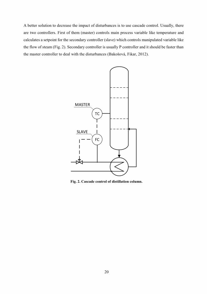
A better solution to decrease the impact of disturbances is to use cascade control. Usually, there
are two controllers. First of them (master) controls main process variable like temperature and
calculates a setpoint for the secondary controller (slave) which controls manipulated variable like
the flow of steam (Fig. 2). Secondary controller is usually P controller and it should be faster than
the master controller to deal with the disturbances (Bakošová, Fikar, 2012).
Fig. 2. Cascade control of distillation column.
TC
FC
MASTER
SLAVE
21
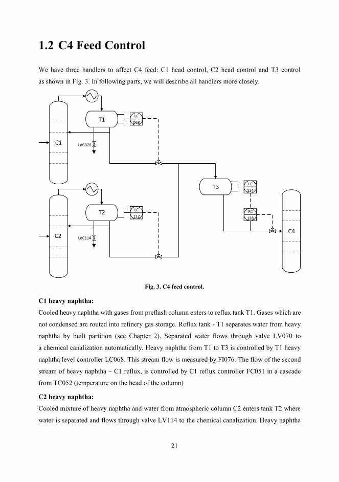
1.2 C4 Feed Control
We have three handlers to affect C4 feed: C1 head control, C2 head control and T3 control
as shown in Fig. 3. In following parts, we will describe all handlers more closely.
Fig. 3. C4 feed control.
C1 heavy naphtha:
Cooled heavy naphtha with gases from preflash column enters to reflux tank T1. Gases which are
not condensed are routed into refinery gas storage. Reflux tank - T1 separates water from heavy
naphtha by built partition (see Chapter 2). Separated water flows through valve LV070 to
a chemical canalization automatically. Heavy naphtha from T1 to T3 is controlled by T1 heavy
naphtha level controller LC068. This stream flow is measured by FI076. The flow of the second
stream of heavy naphtha – C1 reflux, is controlled by C1 reflux controller FC051 in a cascade
from TC052 (temperature on the head of the column)
C2 heavy naphtha:
Cooled mixture of heavy naphtha and water from atmospheric column C2 enters tank T2 where
water is separated and flows through valve LV114 to the chemical canalization. Heavy naphtha
LC
068
LC
112
LdC070
LdC114
LC
124
FC
128
C1
C2C4
T1
T2
T3

22
from T2 to T3 is controlled by T2 heavy naphtha level controller LC112 controller and measured
by FT118.
T3 control:
Heavy naphthas from preflash and atmospheric columns are mixed in tank T3. A mixture of
heavy naphtha (feed to C4) is controlled by flow controller FC128 in a cascade from T3 heavy
naphtha level controller LC124. Heavy naphtha from T3 goes through exchangers to redistillation
column C4 on 27th tray. Products from C4 column are a gas to low pressure gas storage, C5/C6
fraction, light heavy naphtha and heavy naphtha.
C4 feed control issues:
Heavy naphtha flow from T2 to T3 oscillates significantly, for reasons which cannot be resolved.
Due to the current control setup, these fluctuations are transferred downstream to the C4 column.
Fluctuation of feed flow to C4 column causes fluctuation of temperature, which has a negative
impact on quality of heavy naphtha. See Fig. 4, where the blue line is feed flow (t/h) and the red
line is temperature on 24th tray (°C). The purpose of this work will be to propose and implement
control system to mitigate given fluctuations.
Fig. 4. Fluctuations of feed and temperature.

23
2 Modeling of the Tank System
All three tanks (T1, T2and T3) have a similar construction. The difference is only between
construction parameters values. In Fig. 5 we can see the scheme of the horizontal tank.
Construction parameters are in the table below. The tank has rounded ends, but we omitted this
for simplification.
Fig. 5. Tank scheme.
In a table below there are values of construction parameters for T3:
Table 1. Tank parameters.
Parameter Description Value Unit
L the length of the tank 5.803 m
Lw the length of water side 3.375 m
Lg the length of heavy naphtha side 2.428 m
r the radius of the tank 1.184 m
hb the height of the barrier 1.400 m
h0 height of 0% level indication 0.675 m
h100 height of 100% level indication 1.725 m
h100
h0
L
Lw Lg
rhb

24
2.1 Derivation of Model
We need more parameters to derive a model:
Table 2. Model parameters.
Parameter Description Unit
qin (t) input flow to tank m3/h
qout(t) output flow from the tank m3/h
h (t) the height of level in the tank m
ρ density t/m3
min(t) input mass flow to tank t/h
mout(t) output mass flow from the tank t/h
Mass balance:
{input flow to tank} = {output flow from tank} + {accumulation of liquid in tank}
𝑞in = 𝑞out +𝑑𝑉
𝑑𝑡 (2)
The volume of the tank depends on the height of level and the level varies with time. We can
write:
𝑑𝑉(ℎ(𝑡))
𝑑𝑡= 𝑞in(𝑡) − 𝑞out(𝑡) (3)
with initial condition h(0) = hs.
Instead of volumetric flows we rather use mass flows:
𝑑ℎ(𝑡)
𝑑𝑡=
��in(𝑡) − 𝑚out(𝑡)𝑑𝑉(ℎ)
𝑑ℎ𝜌
(4)
The volume of the horizontal tank can be calculated as (King, 2011):
𝑉 = [𝑟2𝑐𝑜𝑠−1 (𝑟 − ℎ
𝑟) − (𝑟 − ℎ)√2𝑟ℎ − ℎ2] 𝐿 (5)
Finally, we have a mathematic model:
𝑑ℎ(𝑡)
𝑑𝑡=
��in(𝑡) − 𝑚out(𝑡)
2𝐿√−ℎ(ℎ − 2𝑟)𝜌 (6)
This calculation assumes a nonlinear relationship between volume and level indication. We
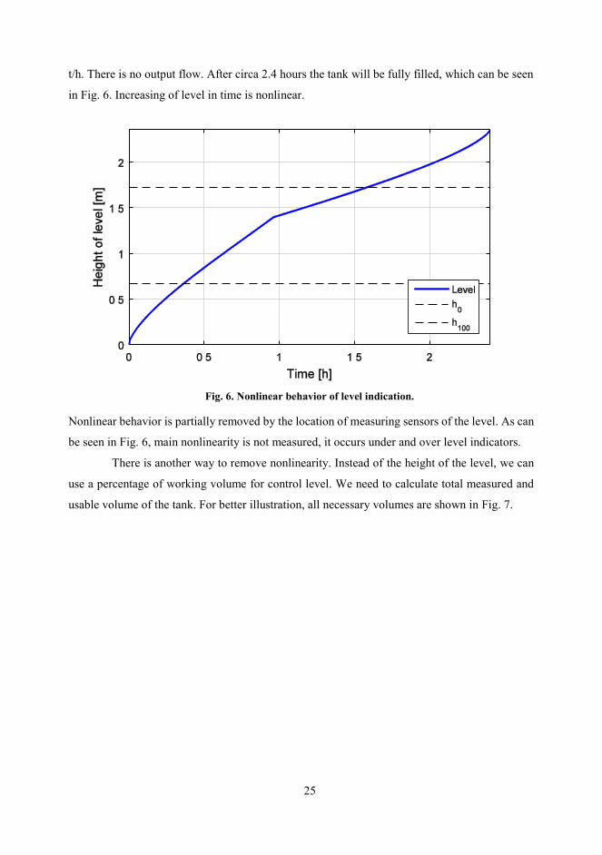
explain this argument in a small experiment. Let’s say h(0) = 0 m and input mass flow min = 5
25
t/h. There is no output flow. After circa 2.4 hours the tank will be fully filled, which can be seen
in Fig. 6. Increasing of level in time is nonlinear.
Fig. 6. Nonlinear behavior of level indication.
Nonlinear behavior is partially removed by the location of measuring sensors of the level. As can
be seen in Fig. 6, main nonlinearity is not measured, it occurs under and over level indicators.
There is another way to remove nonlinearity. Instead of the height of the level, we can
use a percentage of working volume for control level. We need to calculate total measured and
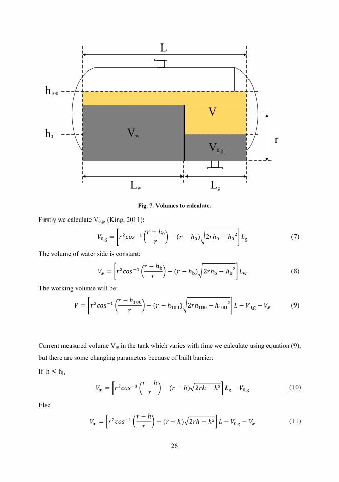
usable volume of the tank. For better illustration, all necessary volumes are shown in Fig. 7.
26
Fig. 7. Volumes to calculate.
Firstly we calculate V0,g, (King, 2011):
𝑉0,g = [𝑟2𝑐𝑜𝑠−1 (𝑟 − ℎ0
𝑟) − (𝑟 − ℎ0)√2𝑟ℎ0 − ℎ0
2] 𝐿g (7)
The volume of water side is constant:
𝑉𝑤 = [𝑟2𝑐𝑜𝑠−1 (𝑟 − ℎb
𝑟) − (𝑟 − ℎb)√2𝑟ℎb − ℎb
2] 𝐿w (8)
The working volume will be:
𝑉 = [𝑟2𝑐𝑜𝑠−1 (𝑟 − ℎ100
𝑟) − (𝑟 − ℎ100)√2𝑟ℎ100 − ℎ100
2] 𝐿 − 𝑉0,g − 𝑉𝑤 (9)
Current measured volume Vm in the tank which varies with time we calculate using equation (9),
but there are some changing parameters because of built barrier:
If h ≤ hb
𝑉m = [𝑟2𝑐𝑜𝑠−1 (𝑟 − ℎ
𝑟) − (𝑟 − ℎ)√2𝑟ℎ − ℎ2] 𝐿g − 𝑉0,g (10)
Else
𝑉m = [𝑟2𝑐𝑜𝑠−1 (𝑟 − ℎ
𝑟) − (𝑟 − ℎ)√2𝑟ℎ − ℎ2] 𝐿 − 𝑉0,g − 𝑉𝑤 (11)
h100
h0
L
Lw Lg
rVw
V0,g
V
27
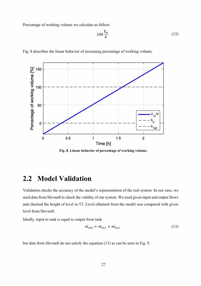
Percentage of working volume we calculate as follow:
100𝑉m
𝑉 (12)
Fig. 8 describes the linear behavior of increasing percentage of working volume.
Fig. 8. Linear behavior of percentage of working volume.
2.2 Model Validation
Validation checks the accuracy of the model’s representation of the real system. In our case, we
used data from Slovnaft to check the validity of our system. We used given input and output flows
and checked the height of level in T3. Level obtained from the model was compared with given
level from Slovnaft.
Ideally, input to tank is equal to output from tank
𝑚out = 𝑚in,1 + 𝑚in,2 (13)
but data from Slovnaft do not satisfy the equation (13) as can be seen in Fig. 9.

28
Fig. 9. Input and output flow comparison.
Based on process data, this is caused by a proportional error on sensors of mass flow of output
from T1 and T2, which sum is input to T3. By using input presented above (min,1 + min,2), the T3
is filled in a few minutes, because input is always bigger than output.
If our input and output mass flows should be equal, we need to multiply outputs flows
from T1 and T2 by constants calculated by regression of process data:
𝑚out = 𝑚in,1 ∙ 1.0303 + ��in,2 ∙ 0.8846 (14)
After this correction output is approximately the same as input (Fig. 10).

29
Fig. 10. Input and output flow comparison after correction.
Now we can validate our model by comparing level from the model and from Slovnaft data,
which is shown in Fig. 11. We succeeded with type of oscillations but it is unstable process,
so every small change can lead to divergence as you can see in Fig. 11 until 15th hour or from
53rd hour.
Fig. 11. Model and Slovnaft level comparison.
30
3 Slovnaft Control System
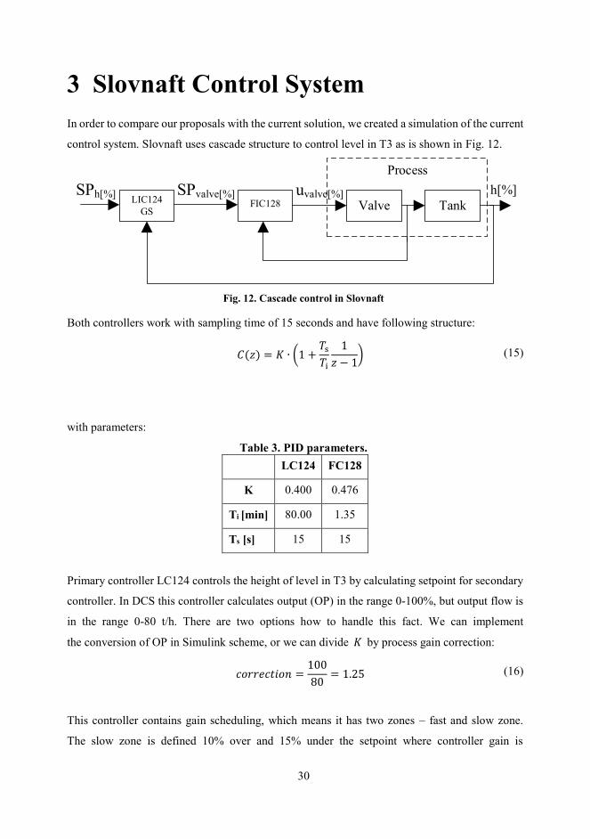
In order to compare our proposals with the current solution, we created a simulation of the current
control system. Slovnaft uses cascade structure to control level in T3 as is shown in Fig. 12.
Fig. 12. Cascade control in Slovnaft
Both controllers work with sampling time of 15 seconds and have following structure:
𝐶(𝑧) = 𝐾 ∙ (1 +𝑇s
𝑇i
1
𝑧 − 1) (15)
with parameters:
Table 3. PID parameters.
LC124 FC128
K 0.400 0.476
Ti [min] 80.00 1.35
Ts [s] 15 15
Primary controller LC124 controls the height of level in T3 by calculating setpoint for secondary
controller. In DCS this controller calculates output (OP) in the range 0-100%, but output flow is
in the range 0-80 t/h. There are two options how to handle this fact. We can implement
the conversion of OP in Simulink scheme, or we can divide 𝐾 by process gain correction:
𝑐𝑜𝑟𝑟𝑒𝑐𝑡𝑖𝑜𝑛 =100
80= 1.25 (16)
This controller contains gain scheduling, which means it has two zones – fast and slow zone.
The slow zone is defined 10% over and 15% under the setpoint where controller gain is
Process
SPh[%]FIC128 Valve Tank
LIC124
GS
h[%]SPvalve[%] uvalve[%]

31
multiplied by factor 0.7. Gain scheduling has been achieved in Simulink using „IF“ block. Fig. 13
shows, how controller switches between proportional gains.
Fig. 13. Gain scheduling.
The secondary controller FC128 controls output flow by operating with a valve on output from
T3. Setpoint for this controller generates primary controller. Performance under PID controller
with Slovnaft parameters is shown in Fig. 14.

32
Fig. 14. Model and Slovnaft PID control performance.
Fig. 15. Detail of control performance.

33
4 Level Control
The aim of this section of work is to design a controller which minimizes oscillations of
the output flow from T3. In this chapter, we will try to propose such controller in the traditional
way, ie. not using APC. There are two methods to design level controllers, tight and averaging
level control. Tight control is for situations when it is more important to hold the level close to
setpoint than maintaining a steadily manipulated flow. We use the second method, averaging
control when it is more important to keep manipulated flow as steady as possible. This can be
achieved by using all working volume of the tank without violating level alarms.
4.1 Parameters for Controller Design
The first step is to determine some necessary parameters as shown in Fig. 16.
Fig. 16. Parameters for controller design.
Working volume (V) was determined in Chapter 2.1. Normally expected flow disturbance (f) can
be obtained from historical data. This disturbance is shown for example in Fig. 14. The smaller
value of f should be chosen when all capacity of the tank is not used. To define how much of tank
capacity can be used, we need parameter d which is a maximal deviation from setpoint to low and
high-level alarm. The last parameter is F, defined as maximum output flow. All parameters are
in Table 4 below.
FI
LC
LHA
LLA
FC
100%
0%
SP
f
d
range=F

34
Table 4. Parameters for controller design.
Parameter Value Unit
f 2.500 t/h
V 6.072 m3
SP 57.50 %
LHA 75.00 %
LLA 40.00 %
d 17.50 %
F 80.00 t/h
4.2 Averaging Level Control
We calculate the smallest possible controller gain (King, 2011):
𝐾min =100𝑓
𝐹𝑑 (17)
As can be seen in Fig. 17, the level does not activate alarms. It was only one model disturbance,
but we need return level to SP considering the next disturbance. For this case, we add integral
action and modify controller gain as (18)
𝐾𝑐 =80𝑓
𝐹𝑑, 𝑇i =
𝑉𝑑
12.5𝑓 (18)
Controller uses parallel form:
𝐶(𝑧) = 𝐾c +𝐾c𝑇s
𝑇i
1
𝑧 − 1
(19)
Input flow was increased as a step change. Manipulated flow was increased as slowly as possible
and it took about 2 hours. Fig. 18 shows the performance of averaging control with designed
controller.

35
Fig. 17. Proportional control only.
Fig. 18. Averaging level control.

36
For better control performance, controller parameters were tuned. Both, calculated and tuned
constants are in Table 5,
Table 5. Calculated and tuned controller constant.
Constant Calculated Tuned
P -0.14 -0.08
I -0.04 -0.10
where P = Kc and I = Kc/Ti.
As can be seen in Fig. 19 manipulated flow oscillates less using averaging control than using
cascade in Slovnaft.
Fig. 19. Averaging control with real data.
37
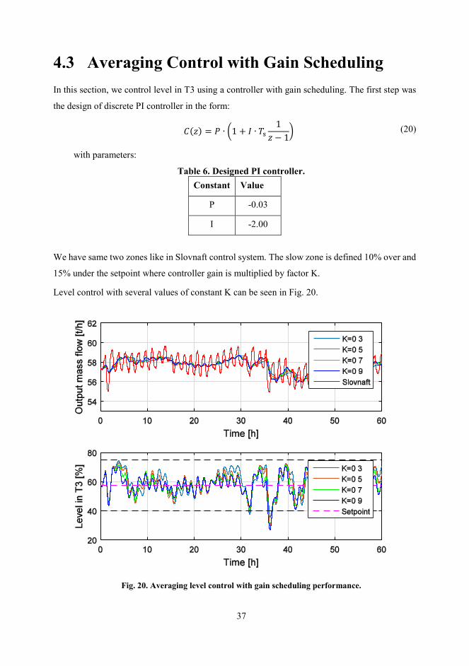
4.3 Averaging Control with Gain Scheduling
In this section, we control level in T3 using a controller with gain scheduling. The first step was
the design of discrete PI controller in the form:
𝐶(𝑧) = 𝑃 ∙ (1 + 𝐼 ∙ 𝑇s
1
𝑧 − 1) (20)
with parameters:
Table 6. Designed PI controller.
Constant Value
P -0.03
I -2.00
We have same two zones like in Slovnaft control system. The slow zone is defined 10% over and
15% under the setpoint where controller gain is multiplied by factor K.
Level control with several values of constant K can be seen in Fig. 20.
Fig. 20. Averaging level control with gain scheduling performance.

38
Detail of control performance:
Fig. 21. Detail of control performance.

39
5 Percentage of Working Volume
Control
This chapter is focused on the percentage of working volume control described in 2.1. Requested
height of level in the tank is recalculated on the percentage of working volume of the tank and this
is setpoint for the controller. At first, we tried it using Slovnaft control scheme. Results are in Fig.
22 and Fig. 23.
Fig. 22. The performance of percentage of working volume control – Slovnaft.

40
Fig. 23. Detail of control performance.
We also used designed averaging controller from chapter 4.2 and controlled percentage of
working volume. By comparing level control and percentage of working volume control we can
see that there are only minimal improvements using second mentioned method. The reason is
simple. Main nonlinearity which occurred in level indication was removed by level sensors
placement. Comparison of these two methods is in Fig. 24 and Fig. 25. A varying percentage of
working volume is in Fig. 26.

41
Fig. 24. The performance of percentage of working volume control – averaging control.
Fig. 25. Detail of control performance.

42
Fig. 26. Percentage of working volume.
To compare which method gives us the smallest oscillation of output flow from T3, we calculated
the sum of squares:
∑(��𝑖,out − 𝑟𝑒𝑓𝑖)2
𝐾
𝑖=1
(21)
where ref is reference curve vector shown in Fig. 27 and K is a number of elements of reference
curve. Calculated values are in Table 7 below. Using averaging level control was a significant
improvement against Slovnaft controllers. Little improvement has been achieved using
percentage of volume instead of level.
Table 7. Control methods comparison.
Control method Sum of squares
Slovnaft controllers 9684
Averaging control - level 2212
Averaging control – percentage of volume 1749

43
Fig. 27. Reference curve.

44
6 Advanced Process Control - RMPCT
Advanced process control (APC) is a wide range of techniques implemented in industrial process
control systems. One of them is multivariable model predictive control. Honeywell has
developed his own application for control of multi-input, multi-output interactive industrial
processes called Robust Multivariable Predictive Control Technology (RMPCT). (Honeywell,
01/2012)
Profit controller (RMPCT) provides control and optimization subject to time varying
constraints. This controller contains a dynamic model of the process from which it predicts future
behavior and determines, how controller´s outputs should look like to achieve setpoints of all
process variables. Sometimes it is sufficient when process variables are within constraints.
RMPCT can achieve good control results even though there are errors in the process model.
(Honeywell, 10/2012)
6.1 Controller Variables
We know three types of variables which uses Profit controller to control the system:
Controlled Variables (CVs): controller tries to keep these variables on a setpoint or
within a range, but in both cases, the constraints have to be satisfied.
Manipulated Variables (MVs): these variables are changed by the controller to
achieve required results with CVs. Of course, all MVs can be changed only within
constraints.
Disturbance Variables (DVs): these variables are measured, but they are not
controlled. They may come from upstream processes and affect CVs. Prediction of the
effects of DVs on CVs can help keep CVs within constraints. (Honeywell, 10/2012)
Using a SISO controller there is only one CV and one MV. The controller looks only at one loop
and does not care about other loops in a system. With RMPCT there are multiple MVs and
multiple CVs. The controller views all variables together as a system and considers effects of all
interactions between MVs and CVs.

45
6.2 Models
Model of the system that uses Profit Controller is built from dynamic sub-processes models
which contain information about behavior between independent variables MVs, DVs and CVs.
Sub-process models are null when there is no physical connection between MV or DV and CV.
Profit controller (RMPCT) uses a generic form of sub-process model, which contains a
number of coefficients whose values we need to find to identify the model. We want to achieve
predicted responses as close as possible to actual process responses.
6.3 Objective Function
To keep CVs on a setpoint or within a range, we need sufficient degrees of freedom. Degrees of
freedom is a number of MVs which are not at a limit minus number of CVs which have setpoints
or which are out of the limits. If the number of degree of freedom is positive or zero, all
constraints of CVs can be satisfied. If the number is negative it is impossible to achieve CV´s
setpoint or keep CVs within a range.
There are some cases when we have more CVs than MVs and it is possible to achieve
setpoints or keep CVs within the range. In these cases, it should be there a sufficient number of
CVs which have only a range instead of the setpoint. (Honeywell, 01/2012)
As an objective function, we consider the linear or quadratic function of any CVs and
MVs or of all of them.
General form:
min 𝐽 = ∑ 𝑏𝑖 ∙ 𝐶𝑉𝑖 + ∑ 𝑎𝑖2 ∙ (𝐶𝑉𝑖 − 𝐶𝑉0,𝑖)
2+
𝑖𝑖
∑ 𝑏𝑗 ∙ 𝑀𝑉𝑗 + ∑ 𝑎𝑗2 ∙ (𝑀𝑉𝑗 − 𝑀𝑉0,𝑗)
2
𝑗𝑗
(22)
where:
b is the linear coefficient
a is the quadratic coefficient
index i belongs to the CVs
index j belongs to the MVs
CV0, MV0 are the desired values
In our case, we consider only quadratic function, because we have setpoint. In the case of control
between limits, we would use the linear function.

46
7 Identification and Controller Design
The major aim of this thesis was to propose and implement APC which will coordinate flows and
levels in given tanks systems in order to mitigate redistillation column feed fluctuations.
Following chapters describe steps of implementation of given APC and its evaluation.
7.1 Data Preparation
For the identification of tanks system using Honeywell Profit Design Studio, we need to get
model data from step responses. These step responses were obtained from Matlab – Simulink
simulations. Before running any simulation or identification we need to classify variables to
controlled, manipulated and disturbance variables as you can see in Fig. 28.
Fig. 28. Classification of variables for APC.
We have two controlled variables (CVs) – percentage of working volume in T1 and T3, two
manipulated variables (MVs) – valve opening from T1 and output flow from T3 and one
disturbance variable (DV) – output flow from T2. Last mentioned disturbance variable can not be
manipulated variable because the valve is sticking. We use a percentage of working volume CVs
instead of raw levels, since this ensures us linear model between MVs and level CVs. Instead of
measured output flow from T1, we use a percentage of opening of the valve. Between valve
CV1
T2
LC068.PV
CV2LC124.PV
MV1LC068.OP
DV1FT118.PV
MV2FC128.SP

47
opening and flow through there is a linear relationship calculated from LC068.OP vs FI076.PV
process data:
Output flow = 0.52*Percentage of opening
After classification of variables, we can achieve step responses. Since the percentage of
working volume (CVs) have linear models to our MVs and we had all necessary data, we could
calculate responses and models theoretically. However in order not to skip Profit Suite
identification we decided to use Matlab-Simulink simulation to get steptest data.
The time period for step responses data is one minute. Step responses were made
in respect to not violating alarms in the tank. Results are shown in Fig. 29. We made steps up and
down due to unstable process. The process will not stabilise by itself after one step change.
Fig. 29. Step responses.
The data were given into Excel template in the form shown below.

48
Fig. 30. Data preparation for PDS.
7.2 Identification
Now we can identify system using Honeywell Profit Design Studio (PDS). We open the PDS and
choose File => New => Model Dev. File (Fig. 31).
Fig. 31. Creating anew model.
Mark all data in created Excel file including headings and select Data operations => Paste from
clipboard. After this, we can see the window shown below (Fig. 32).

49
Fig. 32. Data imported in PDS.
The output from identification is a CVs - MVs/DVs model matrix. We use Finite impulse
response (FIR). FIR step response models are obtained by integrating the finite impulse response
coefficients. These models represent the response of a dependent variable (CV) to a step change
made to an independent variable (MV or DV).Select Identify => Set Overall Options and mark
Finite Impulse Response (FIR). In this window, we can also specify the number of trials.
The trials are partial models in case if we need only a part of all dynamic. For better illustration
see Fig. 33 from another process identification.
50
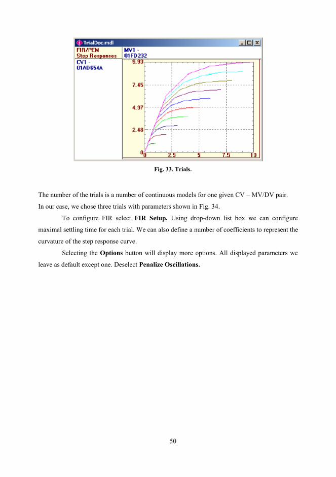
Fig. 33. Trials.
The number of the trials is a number of continuous models for one given CV – MV/DV pair.
In our case, we chose three trials with parameters shown in Fig. 34.
To configure FIR select FIR Setup. Using drop-down list box we can configure
maximal settling time for each trial. We can also define a number of coefficients to represent the
curvature of the step response curve.
Selecting the Options button will display more options. All displayed parameters we
leave as default except one. Deselect Penalize Oscillations.

51
Fig. 34. Overall parameters.
After setting overall options the identification can begin. Select Identify => Fit FIR/PEM/CLid
Models. Double click on sub-process will open dialog box Options per Submodel (Fig. 35). If
there is no physical way, how independent variable – MV/DV can affect CV, mark Null
Sub-Process. In all other sub-process, we mark Integrating Sub-Process.
52
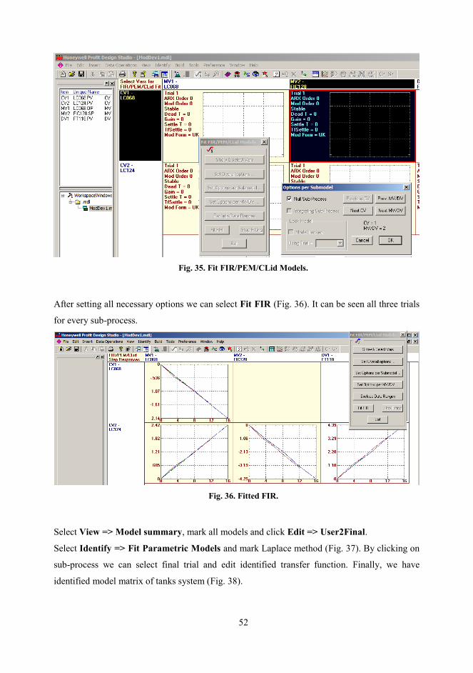
Fig. 35. Fit FIR/PEM/CLid Models.
After setting all necessary options we can select Fit FIR (Fig. 36). It can be seen all three trials
for every sub-process.
Fig. 36. Fitted FIR.
Select View => Model summary, mark all models and click Edit => User2Final.
Select Identify => Fit Parametric Models and mark Laplace method (Fig. 37). By clicking on
sub-process we can select final trial and edit identified transfer function. Finally, we have
identified model matrix of tanks system (Fig. 38).

53
Fig. 37. Editing sub-processes.
Fig. 38. Final trials.
We can illustrate how accurate is our identification by comparing measured CVs with predicted
CVs from identified models: Identify => Select Final Trials, enable Store Predictions and
select Plot Predictions. The result is in Fig. 39.

54
Fig. 39. CVs predictions.
The red line represents measured step responses and the green line is predicted step responses.
As it was mentioned before, it was possible to get models theoretically. Since models are linear
and we know capacity of the tank, slope of the integrator is easily calculated as the ratio of step
change per minute to the capacity of the tank. Models obtained by calculation and by
identification were in coincidence, so based on this and prediction check we can consider, that
models were identified correctly.

55
7.3 Building Controller
Next step is building the controller. At first, we need to build Unified Real Time Platform (URT
Platform). This platform serves to implement real-time APC applications. In PDS we choose
View => Model Summary, mark all models and select Edit => User2Final. Now we can start
with the controller: Build => Controller. It is necessary to generate all setting files choosing
options shown in Fig. 40. Generating setting files.Fig. 40.
Fig. 40. Generating setting files.
Select Build, if an error window appears, just click No (Fig. 41).

56
Fig. 41. Error window.
PDS generates setting files. These files we move to C:\ProgramData\Honeywell\URT\Platforms.
Open Profit Suite Runtime Studio (PSRS): File => New => Profit Controller => Ok (Fig. 42).
Fig. 42. Create a New Application.
We describe general information shown in Fig. 43, choose .xm .xs files generated in the previous
step and .mdl file with our model and click Ok.

57
Fig. 43. General information.
In a Controller section, we describe information as shown in Fig. 44. Again we choose .mdl file
with our model.

58
Fig. 44. Controller.
Fig. 45. Points.

59
Section Points (Fig. 45) is about variables properties. We define engineering units and range of
the variable. Instead of the level, we use a percentage of working volume to calculate output from
the controller. This is a reason why we named our CVs LX instead LC. Part of the Points section
called Detail we set it as in Fig. 46.
Fig. 46. Details.
Connections for Base Level Controls is about what to do with MV´s controller in a case of
shutting down the APC. MV1 switches to the automatic and MV2 switches to the cascade control
(Fig. 47).

60
Fig. 47. Connections for Base Level Controls.
Now we have built Watchdog, which is a kind of small program to check a communication
between APC and our target. We save it like URT Platform, which is ground for APC
coordination.
7.4 Controller Calculations
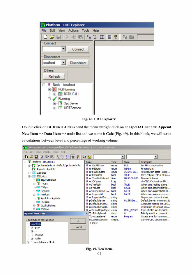
We start URT Explorer and in a left side, there are all platforms (Fig. 48). If our platform is not
activated we can do it by double click on BCDU61L1 => Start Platform.
61
Fig. 48. URT Explorer.
Double click on BCDU61L1 =>expand the menu =>right click on an OpcDAClient => Append
New Item => Data Item => node list and we name it Calc (Fig. 49). In this block, we will write
calculations between level and percentage of working volume.
Fig. 49. New item.

62
Right click on Calc => Append New Item => Profit Suite Block => Profit Toolkit =>
Variable Combinations and we name it Levels. Now we have block for calculations. We need
four calculations. Two of them are for the level in percentage to level in meters calculation and
the rest two are for calculation of the percentage of working volume from a level in the tank.
Right click on Combinations => Properties => Value => Working size = 4. The result is in
Fig. 50.
Fig. 50. Combinations block.
At first, we need to define T1m and T3m. Inputs to these blocks are values of levels in tanks T1
and T3 in percentage. The output from these blocks are levels in meters. I will describe the setup
of combinations blocks on LX068 calculation. The result from this block is the percentage of
working volume in tank T1. The input to this block is level in meters, which is also result from
T1m block. Basically, we need to insert calculations from Chapter 2.1, equations (9),(10)(11).
At first, we define a number of variables necessary for the calculation. LX068 => Number of
Variables => Value => Working value =8, (Fig. 51). Variables are described in Table 8, (Fig.
52).
Table 8. Calculation variables.
Name Description
IV1 Level in the tank
IV2 Radius of the tank
IV3 Length of the tank
IV4 Length of gasoline side
IV5 Volume of unuseful gasoline part
IV6 Volume of water side
IV7 Total useful volume
IV8 Height of barrier

63
Fig. 51. T1 level calculation block.
Fig. 52. Variable names.
Fig. 53. Variable values.

64
After defining variable names, we define their values. Only the first variable IV1 (level in meters)
is changing at a time and it is result from T1m block. We have to connect this variable with
the corresponding result. Right click on Variables => Properties => PerElem IN Con and
choose Type: URT and a Target is the location of T1m result shown in Fig. 54.
Fig. 54. Variable connection.
The last but very important step is to define an equation for calculation with decision rule
described in 2.1. Variables => Equation => Value => Working value. In this box, we write all
decision rules with two equations (Fig. 55).

65
Fig. 55. Equation.
The result from this block is the percentage of working volume in tank T1. The same approach is
used for T3 level calculation.
66
8 Controller Configuration and Strategy
Part of the package that we used – Profit Suite is Profit Suite Operator Station (PSOS). This
software is used for interaction between operator and APC. Here we set controller strategy by
changing of optimization coefficients and limits. Our aim was to ensure, that T2 heavy naphtha
flow fluctuation will be compensated by T1 heavy naphtha flow while levels will be inside limits.
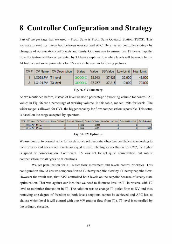
At first, we set some parameters for CVs as can be seen in following pictures.
Fig. 56. CV Summary.
As we mentioned before, instead of level we use a percentage of working volume for control. All
values in Fig. 56 are a percentage of working volume. In this table, we set limits for levels. The
wider range is allowed for CV1, the bigger capacity for flow compensation is possible. This setup
is based on the range accepted by operators.
Fig. 57. CV Optimize.
We use control to desired value for levels so we set quadratic objective coefficients, according to
their priority and linear coefficients are equal to zero. The higher coefficient for CV2, the higher
is speed of compensation. Coefficient 1.5 was set to get quite conservative but robust
compensation for all types of fluctuations.
We set penalization for T3 outlet flow movement and levels control priorities. This
configuration should ensure compensation of T2 heavy naphtha flow by T1 heavy naphtha flow.
However the result was, that APC controlled both levels on the setpoint because of steady state
optimization. That was against our idea that we need to fluctuate level in T1 in reverse with T2
level to minimize fluctuation in T3. The solution was to change T3 outlet flow to DV and thus
removing one degree of freedom so both levels setpoints cannot be achieved and APC has to
choose which level it will control with one MV (output flow from T1). T3 level is controlled by
the ordinary cascade.

67
MVs were configured in following way:
Fig. 58. MV Summary.
Fig. 59. MV Optimize.
Limits were set according to process data and manual limits. In the previous setup MV2 weight
was set, to penalize its movement. However, the strategy was changed and MV weight is not set.
DVs configuration is defined here:
Fig. 60. DV Summary.
There are no limits to set, what comes from nature of DVs.

68
Discussion
After few hours of running APC controller, we have results to show. In Fig. 61 it can be seen the
behavior of levels in tanks before and after the APC was turned on. It was turned at time of 25
hours.
Fig. 61. Levels in tanks.
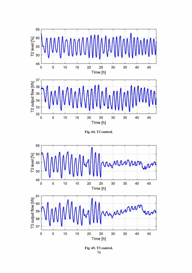
As you can see in Fig. 62 the APC try to fluctuate level in T1 in reverse with T2 level. This
control causes less fluctuation in T3 level. In Fig. 63, Fig. 64, Fig. 65 there are all tanks – levels
and output flows. T1 level oscillates between 45 and 65%. In order to set speed and capacity of
T1 compensation CV1 quadratic coefficient and limits can be changed. The higher quadratic
coefficient for CV1 means faster compensation. Wider limits for CV1 mean higher capacity for
compensation. For the purpose of analysis, it would be good to show results for different
configurations. However this would mean upset for normal operation, so we minimized the time
for configuration and there are no relevant data to show. For this reason, we did not verify our
assumptions about effects of changes CV1 parameters.

69
Fig. 62. Detail of control performance.
Fig. 63. T1 control.
70
Fig. 64. T2 control.
Fig. 65. T3 control.

71
Stabilisation of level in T3 implied stabilisation of output flow from T3, which is a feed flow for
a C4 distillation column. The bottom temperature in the column also stabilised - Fig. 66.
According to the conservative assumption, at least 60% temperature oscillation was removed.
Fig. 66. Final results.
There was no significant change in processes upstream after turned on APC. This is presented
in Fig. 67. As you can see there is no change caused by APC after 25th hour.
Fig. 67. The temperature in C1 column.

72
For illustration there is graph from Uniformance Process History Database (Honeywell) used in
Slovnaft:
Fig. 68. Uniformance PHD trend.
Table 9. The meaning of signals.
Signal Meaning Unit
AVD.LC068.PV Level in T1 %
AVD.LC068.OP Output from controller to valve %
AVD.LC112.PV Level in T2 %
AVD.LC112.OP Output from controller to valve %
AVD.LC124.PV Level in T3 %
AVD.FC128.SP Output from controller to valve t/h
AVD.TC228.PV Temperature in C4 column °C
AVD.TC052.PV Temperature in C1 column °C

73
Conclusion
The aim of this work was to reduce the fluctuation of output flow from a system of three
horizontal cylindrical tanks. This system of tanks is a part of distillation unit in Slovnaft called
BCDU6. Fluctuation of output flow disturbs downstream operations.
Our first task was to derive a mathematical model of horizontal cylindrical tank. There
was an interesting fact that inside each tank is a barrier used for dividing gasoline from water. In
this first part, we used mainly MATLAB with Simulink. After deriving model, we validated it
and continued with control design. We focused only on the last tank T3. At first, we tried to
reproduce Slovnaft control system of level – cascade control. Slovnaft engineers tried to reduce
non-linearity of the system using gain scheduling as we did. Next work was about developing our
own control strategy to minimize fluctuation of output flow. We used a strategy called averaging
level control. This strategy is based on an idea that we can use all possible volume of the tank to
maintain output flow as steady as possible. Using this strategy we reduced fluctuation by half.
The stronger improvement we achieved using tuned PI controllers with gain scheduling. The last
strategy that we tried by simulations was a percentage of working volume control instead of level.
Using this strategy makes our system linear which is better for control. This strategy was also the
basis for APC control in the second part.
The second part was about APC controller design. We used Profit Suite from Honeywell
which contains several types of software for design and application of APC controller. The first
step was the identification of system. We had to classify variables and did some step tests. Step
tests we did in MATLAB – Simulink and data were exported into Profit Design Studio. Here, we
investigated how depended variables (MVs, DVs) affect independent variables (CVs). We
constructed a model matrix which contains all sub – processes. In the next step, we built URT
Platform which serves to implement APC applications. In URT Explorer we defined necessary
calculations to convert level into a percentage of working volume. The last thing that we had to do
was running a controller and define limits and some another parameter for variables. After
running designed controller for few hours, significant progress has been made in output flow
fluctuation. Reducing of output flow fluctuation reduced also fluctuation of temperature (at least
60%) in the next distillation column, which has a positive impact on operations conducted
downstream. The controller was accepted by unit staff and they use it. Since the model is linear
and it can be theoretically calculated, our solution is easily transferable to other tank systems.

74
Resumé
Táto diplomová práca sa zaoberá návrhom a implementáciou riadenia sústavy troch zásobníkov
kvapaliny v rafinérii Slovnaft a.s. Jedná sa o prevádzku BCDU6 na ktorej prebieha atmosférická
a vákuová destilácia ropy za vzniku produktov. Spomínanú sústavu zásobníkov kvapaliny tvoria
valcové zásobníky umiestnené horizontálne. Prvé dva (T1, T2) zachytávajú produkt
z rektifikácie, ich výstupné prúdy sa spájajú a tvoria vstup do tretieho zásobníka (T3), ktorý
zadržiava nástrek pre vákuovú kolónu C4. Výstupný prietok z T2 kolíše, a tento fakt spôsobuje
kolísanie výšky hladiny v T3, výstupného prietoku z T3 a následne aj teploty v kolóne C4. To má
za následok nepriaznivé podmienky pre riadenie a samotný chod kolóny. Cieľom tejto práce bolo
stabilizovať kolísanie hladiny v T3 a tým aj kolísanie výstupného prietoku z T3.
Prvá časť práce bola zameraná na modelovanie systému, teoreticky návrh riadenia
a overenie pomocou simulácii v programe MATLAB – Simulink. Prvým krokom bolo získanie
matematického modelu horizontálneho valcového zásobníka kvapaliny. Všetky tri zásobníky
mali rovnakú geometriu, líšili sa len veľkosťou. Zaujímavosťou pri týchto zásobníkoch bola
zabudovaná prepážka vo vnútri zásobníka, ktorá slúžila na oddeľovanie zvyškovej vody
v produkte rektifikácie. Odvodený matematický model bol nakoniec validovaný pomocou dát
poskytnutých spoločnosťou Slovnaft a.s.
Pri teoretickom návrhu riadenia sme sa zamerali na zásobník T3. Slovnaft riadi hladinu
v T3 pomocou kaskádovej regulácie PI regulátormi. Výška hladiny v zásobníku je nelineárny
systém, čomu mal v riadení dopomôcť gain scheduling.
Po úspešnom odsimulovaní riadiaceho systému používaného rafinériou Slovnaft sme sa
zamerali na vytvorenie vlastnej stratégie riadenia, ktorá by mala znížiť kolísanie výstupného
prietoku z T3. Stratégia sa nazýva „Averaging level control“. Hlavnou myšlienkou tejto stratégie
je využiť celý možný objem zásobníka bez dosiahnutia alarmov, kedy by sa mal výstupný prietok
v značnej miere ustáliť. Touto metódou sa podarilo dosiahnuť menšie kolísanie výstupného
prietoku približne o polovicu. Ďalšie zlepšenie bolo pozorovateľné ladením regulátorov
a pridaním gain scheduling-u. Poslednou alternatívou, ktorú sme simulovali bola metóda, pri
ktorej namiesto výšky hladiny v zásobníku riadime percento objemu zaplnenia zásobníka. Ako
už bolo spomenuté, výška hladiny v našom zásobníku je nelineárny systém, čo neplatí o percente
objemu. V tomto prípade bolo dôležité zásobník rozdeliť na niekoľko častí a vypočítať ich
objem. Následne sme podľa rovníc v kapitole 2.1 z výšky hladiny vedeli vypočítať percento
75
zaplnenia objemu zásobníka. Aj táto metóda priniesla úspech v podobe zmenšeného kolísania
výstupného prietoku zo zásobníka T3.
Druhá časť bola venovaná návrhu a implementácii APC regulátora. Používali sme
softwarový balík Profit Suite od Honeywellu, ktorý mal mnoho súčastí. Najprv bolo potrebné
rozdeliť premenné na riadené (CV): výšky hladín v zásobníkoch T1 a T3, riadiace (MV):
výstupné prietoky zo zásobníkov T1 a T3 a poruchové (DV): výstupný prietok z T2. Výstupný
prietok z T2 bol zaradený medzi poruchové veličiny kvôli zadrhávaniu ventilu, kedy nie je možné
ovládať ho pre potreby riadenia. V ďalšom kroku sme pristúpili k identifikácii systému. Na
začiatku bolo potrebné vykonať skokové zmeny alebo tzv. steptesty, kde sme sa snažili zistiť
vplyv riadiacich a poruchových premenných (MV, DV) na riadené premenné (CV). Tieto
steptesty sme robili simulačne v programe MATLAB - Simulink a vygenerované dáta sme
spracovali v programe Profit Design Studio. Výsledkom bola modelová matica zložená
z jednotlivých čiastkových procesov. V ďalšom kroku sme vytvorili URT Platformu, ktorá slúži
na implementáciu APC aplikácii. Pri vytváraní APC regulátora sme sa rozhodli použiť metódu
riadenia percenta objemu zaplnenia spomínanú v prvej časti tejto práce. Výpočty potrebné na
prepočet výšky hladiny na percento zaplnenia objemu zásobníka sme definovali v programe URT
Explorer.
Posledným krokom bola implementácia vytvoreného APC regulátora. APC regulátor
bol nahraný do systému a boli vykonané určité nastavenia v rozhraní pre operátorov – Profit Suite
Operator Station. Po spustení navrhnutého regulátora a následnej niekoľko hodinovej prevádzke
bolo vidieť, že výška hladiny v zásobníku T1 ako aj jeho výstupný prietok začali výrazne kolísať.
Pomocou tohto rozkolísania hladiny v T1 sa znížilo kolísanie hladiny v T3, jeho výstupný prietok
a následkom toho aj kolísanie teploty v kolóne C4 o najmenej 60%. Regulátor bol akceptovaný
prevádzkou a používa sa. Pretože model je lineárny a je ho možné vypočítať teoretický, je naše
riešenie ľahko prenosné na iné sústavy zásobníkov.

76
Bibliography
Bakošová, M. – Fikar, M. 2012. Riadenie procesov. Bratislava: Nakladateľstvo STU, 2012. ISBN
978-80-227-3763-0.
Liptak, B. 2002. Instrument Engineers’ Handbook, Process Control and Optimization.
CRC Press, Boca Raton, 4 edition, 2006. ISBN 978-0-84931-081-2.
Mikleš, J. – Fikar, M. 2007.Process Modelling, Identification, and Control. Berlin Heidelberg:
Springer Berlin Heidelberg New York, 2007. 480 s. ISBN 978-3-540-71969-4.
King, M. 2011. Process Control: A Practical Approach. Chichester, UK: Wiley& Sons, 2011.
ISBN9780470975879
Honeywell. 10/2012. Advanced Process Control - Profit Controller – Designers Guide.
Honeywell. 1/2012. Advanced Process Control - Profit Controller – Concepts Reference Guide.