slow-onset enzyme inhibition and inactivationslow-onset enzyme inhibition and inactivation antonio...

��

Slow-onset Enzyme Inhibition and

Inactivation

Antonio Baici

Department of Biochemistry, University of Zurich,Winterthurerstrasse 190, CH-8057 Zurich, Switzerland

E-Mail: [email protected]

Received: 16th February 2012/Published: 15th February 2013

Abstract

Interactions between modifiers and enzymes can either occur rapidly,

on the time scale of diffusion-controlled reactions, or they can be slow

processes observable on the steady-state time scale. Slow interactions

in hysteretic enzymes serve to dampen cellular responses to rapid

changes in metabolite concentration as part of regulatory mechanisms.

Naturally occurring inhibitors of several enzymes, such as the macro-

molecular proteinaceous inhibitors of peptidases, may act slowly when

forming complexes with their targets. To allow physiologically mean-

ingful rates of enzyme inhibition, the modifier concentration is kept at

high levels in nature but problems arise when these levels drop for

some reason. The slow-onset inhibitory behavior of enzyme modifiers

used as drugs may represent a handicap if their concentration at the

target site is insufficient and/or the kinetic constants are inadequate to

warrant pharmacologically meaningful rates of enzyme inhibition. A

truthful knowledge of mechanisms and kinetic constants of such sys-

tems is mandatory for making predictions on the efficiency of the

modifiers in vivo.

Introduction

Slow interactions in enzymology gained popularity after Frieden coined the term hysteretic

enzymes for ‘‘... those enzymes which respond slowly (in terms of some kinetic character-

istic) to a rapid change in ligand, either substrate or modifier, concentration’’ [1].

55

http://www.beilstein-institut.de/escec2011/Proceedings/Baici/Baici.pdf

Experimental Standard Conditions of Enzyme Characterization

September 12th – 16th, 2011, Rudesheim/Rhein, Germany

Frieden also derived an integrated rate equation, see equation (1) below, which relates the

increase of product concentration with time. This equation was later shown to apply to a vast

group of enzymatic mechanisms, whether or not enzyme hysteresis was involved, and the

necessary mathematical background for inhibitors was further developed by Cha [2 – 4] and

Morrison et al. [5 – 7].

Reversible enzyme inhibitors have been classified by Morrison in four categories (Table 1)

depending on the rate of formation of their complexes with enzymes [5]. There are many

instances in which the binding step of modifiers to enzymes occurs rapidly, whereas the

sluggishness of the process is due to events other than the formation of the first complex. For

this reason, the more general expression slow-onset inhibition will be used in place of slow-

binding inhibition. The term ‘slow’ is vague as the time taken by these reactions varies from

seconds to hours. However, it is generally agreed that slow-onset inhibition represents

transient kinetics observed on the steady-state time scale and that the slowness of inhibition

is understood in terms relative to the catalytic step, which is usually a faster process. There is

no clear demarcation between the slow and fast categories in Table 1. For classical inhibitors

the condition [I] » [I]t (the subscript means total concentration) could be trusted if it were not

for the relative magnitudes of [E]t, [I]t and Ki, which are not considered in Morrison’s

classification. In fact, a classical inhibitor can manifests tight-binding properties if [E]t is

comparable in magnitude to Ki. On the other hand, typical high-affinity inhibitors show their

efficiency already for [I]t [E]t at low enzyme concentrations to meet the condition [I]t [E]tKi. Then, the relationships for the tight-binding and the slow, tight-binding classes of

inhibitors in Table 1are better appreciated with the modification [I]t [E]t and Ki in place

of [I]t [E]t.

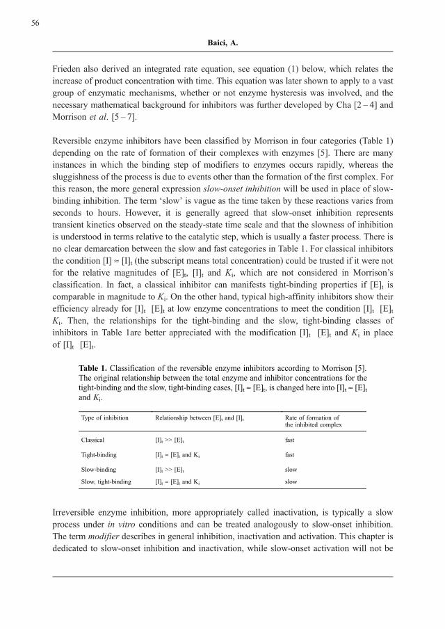
Table 1. Classification of the reversible enzyme inhibitors according to Morrison [5].

The original relationship between the total enzyme and inhibitor concentrations for the

tight-binding and the slow, tight-binding cases, [I]t » [E]t, is changed here into [I]t » [E]tand Ki.

Type of inhibition Relationship between [E]t and [I]t Rate of formation ofthe inhibited complex

Classical [I]t >> [E]t fast

Tight-binding [I]t » [E]t and Ki fast

Slow-binding [I]t >> [E]t slow

Slow, tight-binding [I]t » [E]t and Ki slow

Irreversible enzyme inhibition, more appropriately called inactivation, is typically a slow

process under in vitro conditions and can be treated analogously to slow-onset inhibition.

The term modifier describes in general inhibition, inactivation and activation. This chapter is

dedicated to slow-onset inhibition and inactivation, while slow-onset activation will not be

56

Baici, A.

treated. Steady-state and pre-steady-state equations for slow-onset activation have been

derived by Hijazi and Laidler [8], and an overview of hysteretic, allosteric activators has

been published by Neet et al. [9].

General Aspects of Slow-onset Inhibition

There are several reasons why an inhibitor acts ‘slowly’, including (1) the existence of an

intermediate whose structure recalls that of the transition state; (2) the inhibitor equilibrates

rapidly between two or more forms, one of which makes up only a small proportion of all

forms and interacts with the enzyme; (3) binding of the modifier to the enzyme to form an

intermediate adsorption complex is a fast process, which is followed by a slow structural

rearrangement to a second inhibitory complex; (4) only a rare form of the enzyme, which

equilibrates between conformers, interacts with the modifier; (5) more trivially, it may be

impossible to achieve sufficiently high modifier concentrations so that the rate of the second-

order association reaction with enzyme is slow. The information supplied by the analysis of

the transient phase in slow-onset inhibition experiments is superior to that gained from

steady-state data because the exponential approach to steady-state can be used for

calculating at least some individual rate constants for the inhibitory steps. The mechanism

of inhibition and kinetic constants can be extracted from data either using integrated rate

equations, when available, or by numerical integration.

For some mechanisms, integrated rate equations can be derived under restrictive assump-

tions but this is not always possible. The assumptions require [S] » [S]t and [I] » [I]t, which

means [S]t, [I]t >> [E]t, i. e. experiments must be properly designed to avoid excessive

substrate turnover (say £ 10%) and to circumvent tight-binding between enzyme and inhi-

bitor. In the presence of a slow-onset inhibitor, an enzyme-catalyzed reaction in which

substrate is transformed into product (P) can be described by Frieden’s equation mentioned

above, which reads

½P� ¼ �st þ�z��s�

1� e��t� �

þ d,(1)

where vs and vz are the velocities at steady-state and at time zero, respectively, and l is the

frequency constant of the exponential phase with reciprocal time as dimension. The para-

meter d, for displacement, was added to the original equation to account for any non-zero

value of [P] or background of measured signal proportional to it at time zero. If an integrated

rate equation exists and experiments can be set up to fulfill the assumptions, the equation

can be fitted to progress curves by non-linear regression. In several cases, unambiguous

diagnosis of the mechanism is possible by extracting the information contained in the

expressions of the parameters vs, vz and l. These are functions of inhibitor and substrate

57

Slow-onset Enzyme Inhibition and Inactivation

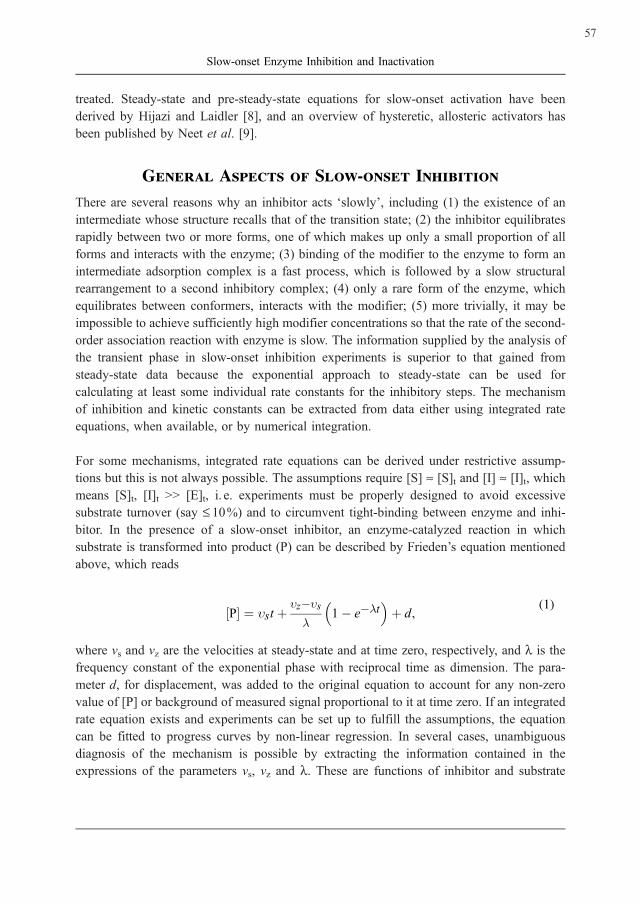
concentrations for a given mechanism and allow the calculation of rate constants. The

graphical representation of slow-onset inhibition according to equation (1) is shown in

Figure 1.

Figure 1. Progress curves for a generic slow-onset inhibition mechanism. The curve in

(b) is obtained when substrate and inhibitor are mixed and reaction is started by

adding enzyme. Curve (c) represents a reaction started by adding substrate to enzyme

and inhibitor that had been preincubated for a sufficiently long tome to allow complex

formation. The dashed line (a) is the tangent at time zero for curve (b) and dashed line

(d) is the corresponding tangent for curve (c).

All mechanisms discussed below are drawn as the simplest one-substrate/one-product reac-

tion for purely practical reasons with the implicit agreement that the same mechanisms can

be applied to multi-reactant enzymes. For instance, in the case of a two-substrate/two-

product enzymatic reaction, one substrate is kept at a constant concentration (not shown in

the scheme) while the concentrations of the second substrate and inhibitor are varied. The

measurements are then repeated exchanging the roles of the varied substrate.

The most frequent mechanism of slow-onset inhibition, both among naturally occurring and

synthetic inhibitors, is of the linear competitive type. A general form is shown in Scheme 1,

panel M11, in which no assumptions are made about the relative rates of equilibration of the

two inhibitory steps. For this mechanism, a progress curve consisting of a double exponen-

tial followed by a linear steady-state release of product is expected but the derivation of an

integrated rate equation is bound to restrictions, of which the absence of tight-binding

between enzyme and inhibitor is the most important. However, it is right M1 in Scheme 1

that is often characterized by tight-binding.

58

Baici, A.

1 Reaction mechanisms, labeled Mx, where x is a progressive number, are grouped in this chapter ascomposite schemes to allow easier finding and cross-referencing

Scheme 1. Mechanisms giving rise to slow-onset inhibition. The labels M1 through

M12 are introduced for facilitating cross-referencing, e.g. M3 is read ‘mechanism 3’.

E = enzyme, S = substrate, P = product, I = inhibitor. The steps labeled slow indicate

qualitatively their relative rate of equilibration with respect to the other steps, which

are assumed to be much faster. EI represents an adsorptive complex, while E.I, *E.I,E’.I, E.Ir, ES.I and ES.S denote reversible, non-covalent complexes. The numbers

identifying kinetic constants of similar paths in diverse mechanisms are the same.

The first approach for analyzing the general mechanism M1 consists in fitting the generic

equations (2) and (3) to progress curves and in evaluating which equation produces the best

fit.

Y ¼ A1 1� e��1t� �

þ kt þ d (2)

Y ¼ A1 1� e��1t� �

þ A2 1� e��2t� �

þ kt þ d (3)

59


Y is a signal proportional to product concentration, A1 and A2 represent amplitudes of the

exponential phases, l1 and l2 are frequency constants, k is the slope of the straight line

following the exponentials and d the value of Y at t = 0. If equation (3) fits data better than

equation (2), any further use of equation (1) for non-linear regression analysis is discour-

aged. Instead, numerical integration is the method of choice in this case. However, even if

the restrictions mentioned above can be avoided, this powerful approach may fail to extract

the information from progress curves if l1 and l2 are coupled. That is to say, if both l1 andl2 contain the rate constants of the forward and reverse inhibitory reactions, the two steps of

M1 cannot be separated from one another because they are ‘mixed together’. Without

analyzing in full the complexity of this system, such problems arise when the values of

k73 and k4 are similar. Simulations of progress curves for this general slow-onset inhibition

mechanism with various combinations of rate constants, reveals that the distinction between

single exponential and double exponential reaction profiles is often very subtle and can be

disclosed only after accurate statistical analysis. Fitting equations (1) or (2) generates pro-

gress curves that, by sight, appear nicely superimposed to data, though with worsening of

the fit in dependence on inhibitor concentration if a single exponential is fit where a double

exponential would better do the job. Introducing noise in the artificial data to simulate

experimental error renders this distinction even more difficult and sometimes impossible.

Yet, the most significant detail is that the kinetic constants calculated by fitting a single

exponential equation to a biexponential progress curve can deviate considerably from the

true values even if the fitted curve, as judged by inspection, appears to be almost perfect. It

is difficult to ascertain from hundreds of reports in the literature whether the most appro-

priate model was fit to data because the overwhelming majority of published slow-onset

inhibition cases were directly addressed to two variants of the general mechanism M1,

namely M2 and M3 in Scheme 1, which can be analyzed with the monoexponential equation

(1). These mechanisms are discussed in the next section.

A suggested approach to data analysis for the general mechanism M1 by numerical integra-

tion is shown in Figure 2. To appreciate the efficiency of the method, artificial data were

simulated and random scatted was added to mimic experimental error. Two sets of fake data

were produced, one for reactions started by adding enzyme (panel a) and another for

reactions started with substrate (panel b). The idea is that data set (a) should represent more

closely the association process, while data set (b) should give more information on the

dissociation of the EI and E.I complexes. The set of differential equations for M1 was then

globally fitted to all data by a combination of numerical integration and non-linear regres-

sion using KinTek software [10, 11]. When the kinetic constants k3, k73, k4 and k74 were

allowed to float freely during the global fit, it was impossible to obtain a unique solution; the

values depended very much from the initial guesses and diverged considerably from the

theoretical values used to generate the fake data. Data set (b) was then excluded from global

fitting and only set (a) was analyzed in a first iteration until stable values of k3 and k73 were

obtained. After constraining k3 and k73 to vary in a constant ratio, global fit was performed

with data sets (a) and (b), which provided four kinetic constants very close to their

60

Baici, A.

theoretical values. Although the satisfactory overlap between data and best fits in Figure 2 is

not yet a guarantee that the fits truly represent the system, running the FitSpace explorer [10]

confirmed that all parameters were well constrained by data.

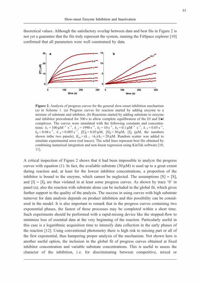
Figure 2. Analysis of progress curves for the general slow-onset inhibition mechanism

(a) in Scheme 1. (a) Progress curves for reaction started by adding enzyme to a

mixture of substrate and inhibitor. (b) Reactions started by adding substrate to enzyme

and inhibitor preicubated for 300 s to allow complete equilibration of the EI and E.Icomplexes. The curves were simulated with the following constants and concentra-

tions: k1 = 100mM71 s71, k71 = 1990 s71, k2 = 10 s

71, k3 = 0.1mM71 s71, k73 = 0.05 s71,

k4 = 0.04 s71, k74 = 0.005 s71, [E]t = 0.05mM, [S]t = 30mM, [I]t (mM, the numbers

shown inthe two panels), Km = (k71 +k2)/k1 = 20mM. Random scatter was added to

simulate experimental error (red traces). The solid lines represent best fits obtained by

combining numerical integration and non-linear regression using KinTek software [10,

11].

A critical inspection of Figure 2 shows that it had been impossible to analyze the progress

curves with equation (1). In fact, the available substrate (30mM) is used up to a great extent

during reaction and, at least for the lowest inhibitor concentrations, a proportion of the

inhibitor is bound to the enzyme, which cannot be neglected. The assumptions [S] » [S]tand [I] » [I]t are thus violated in at least some progress curves. As shown by trace ‘0’ in

panel (a), also the reaction with substrate alone can be included in the global fit, which gives

further support to the quality of the analysis. The success in using curves with high substrate

turnover for data analysis depends on product inhibition and this possibility can be consid-

ered in the model. It is also important to remark that in the progress curves containing two

exponential phases, the fastest of these processes may be completed within a short time.

Such experiments should be performed with a rapid-mixing device like the stopped-flow to

minimize loss of essential data at the very beginning of the reaction. Particularly useful in

this case is a logarithmic acquisition time to intensify data collection in the early phases of

the reaction [12]. Using conventional photometry there is high risk to missing part or all of

the first exponential, thus hampering proper analysis of the mechanism. Not shown here is

another useful option, the inclusion in the global fit of progress curves obtained at fixed

inhibitor concentration and variable substrate concentrations. This is useful to assess the

character of the inhibition, i. e. for discriminating between competitive, mixed or

61


uncompetitive inhibition. Published papers on ‘linear competitive’, slow-onset inhibition

deserve as a remark that the competitive nature of inhibition was not always ascertained

and analysis was performed by taking M2 or M3 in Scheme 1 for granted.

Specific Cases of Slow-onset Inhibition

For all mechanisms discussed in this section, the integrated rate equation and the parameters

therein presume the absence of inhibitor depletion after binding to the enzyme. This can

experimentally be avoided if [E]t can be maintained at least one order of magnitude lower

than [I]t. Mechanisms M2 to M12 in Scheme 1 have in common the same integrated rate

equation (1) but in some cases characteristic combinations of the expressions for vs, vz and l.M2 and M3 can be distinguished from one another because l depends linearly on [I] for M3

and hyperbolically for M2, while vz depends hyperbolically on [I] in mechanism M2 while it

is independent of [I] in M3 [equation groups (4) and (5)]. The kinetic constants for M2 can

be calculated by non-linear regression analysis of l versus [I], with k74 representing the

value of l extrapolated for [I] = 0, and (k4 + k74) as the asymptote of l for [I]?¥. From the

expression of vz and vs and the known value of [S] and Km, Ki and the overall inhibition

constant Ki* can be extracted. Analogously for M3, k73 is calculated as the intercept and k3

from the slope of a plot of l versus [I].

�z ¼V S½ �

Km1þ I½ �Ki

� �þ S½ �

; �s ¼V S½ �

Km1þ I½ �K�i

� �þ S½ �

; ðM2Þ

� ¼ k�4 þk4 I½ �

Ki1þ S½ �Km

� �þ I½ �

; Ki ¼k�3k3

;K�i ¼ Kik�4

k4þk�4

� � (4)

�z ¼ �0 ¼V S½ �

Kmþ S½ �; �s ¼

V S½ �

Km 1þI½ �Ki

� �þ S½ �

; ðM3Þ

� ¼ k�3 þk3 I½ �

1þS½ �Km

; Ki ¼k�3k3

(5)

M4 and M5 represent ‘inhibitors’ that are in reality substrates. At first sight they can be

misidentified as true inhibitors because, for a given extent of time, progress curves are the

same as those shown in Figure 1b. The expressions of vs, vz and l are given in the equation

groups (6) and (7), from which it is seen that discrimination between M2 versus M4 and M3

versus M5 is impossible using the dependence of vz, vs and l upon [I] because the shapes of

these plots are the same. However, if the reaction is started by adding substrate (curve c in

62

Baici, A.

Figure 1), the slope of the linear part of the curve is independent of the preincubation time

between enzyme and inhibitor for M2 and M3 while this increases with increasing

preincubation time for M4 and M5. This because formation of I* reduces the amount of I

that can react with the enzyme to form inhibited complex(es) thus favoring substrate turn-

over. For integrating the rate equations of M4 and M5 the additional assumption [I*] << [I]tis necessary, meaning that equation groups (6) and (7) are valid only if [I]t is sufficiently

large and the measuring time sufficient short to satisfy this condition. The kinetic constants

for M4 and M5 can be calculated likewise their respective counterparts M2 and M3, with the

difference that only the sums (k74 + k5) can be calculated for M4 and (k73 + k5) for M5, not

the individual values. These represent the net ‘off’ constants of the E.I complex. Examples

of M4 and M5 can be found among polypeptides and proteins that bind to peptidases.

Depending on the conditions, they can behave as inhibitors or can be cleaved as substrates

as seen in the interaction between the thyroglobulin type-1 domain and the cysteine pepti-

dase cathepsin L [13], which occurs according to mechanism M4. Although progress curves

were shown without fitting to a particular equation, the slow-onset inhibitory interaction

between Factor Xa and the leech-derived inhibitor antistasin appears to be a further example

of mechanism M4 [14].

�z ¼V S½ �

Km 1þI½ �Ki

� �þ S½ �

; �s ¼V S½ �

Km 1þI½ �

K�i;temp

� �þ S½ �

; ðM4Þ

� ¼ k�4 þ k5 þk4 I½ �

Ki 1þS½ �Km

� �þ I½ �

; Ki ¼k�3k3

;K�i;temp ¼ Kik�4þk5

k4þk�4þk5

(6)

�z ¼ �0 ¼V S½ �

Kmþ S½ �; �s ¼

V S½ �

Km 1þI½ �

K�i;temp

� �þ S½ �

; ðM5Þ

� ¼ k�3 þ k5 þk3 I½ �

1þS½ �Km

; Ki;temp ¼k�3þk5

k3

(7)

The two particular cases of slow-onset inhibition M6 and M7 can be observed if an enzyme

exists in equilibrium between different conformations and only one of these binds the

inhibitor. The two mechanisms differ for the relative positions of the slow and fast steps.

In M6 equilibration between two enzyme forms occurs slowly and only the state labeled *E

reacts with the inhibitor. Although inhibitor binding may occur at the rate of diffusion, the

overall inhibition process is slow because of the limited availability of the *E-form (the

inhibitor ‘must wait’ for it). This mechanism it is likely to occur with enzymes that exist in

distinct conformational states. M6 can be distinguished for the characteristic dependence of

l on [I], which is a concave-up hyperbola (l decreasing for increasing [I]) as shown in the

63


equation group (8). While this allows the determination of k6 and k76, it must be noted that

M6 is a pretty complex mechanism because, depending on the equilibrium between E and

*E, progress curves can show a lag both in the presence and in the absence of the inhibitor

and vz may or may not depend on [I] [6, 15].

In M7 the enzyme isomerizes in a fast process but inhibition proceeds slowly because the

inhibitor can react only with a rare form E’. Since l for M7 is a linear function of [I], the

mechanism cannot be distinguished from M3 on the basis of this parameter, and also vz and

vs are the same as for M3. In this case other sources of information, such as knowledge of

enzyme structure from crystallography or different spectroscopic properties of E and E’,

must be invoked.

� ¼k6

1þS½ �Km

þk�6

1þI½ �Ki

; Ki ¼k�3k3

ðM6Þ (8)

� ¼ k�31þ

S½ �Km

þI½ �Ki

1þS½ �Km

; �z and �s as in M3 ðM7Þ

Km ¼k�1þk2ð Þ k7þk�7ð Þ

k1k7; Ki ¼

k�3ðk7þk�7Þk3k7

(9)

M8 is analogous to M7 but in this case slow-onset inhibition is due to equilibration of the

inhibitor between different molecular forms of which only a rare species reacts with the

enzyme. A well-documented case of M8 is the inhibition of cathepsin B by the peptide

aldehyde leupeptin [16, 17]. The slow-onset inhibitory behavior of this system, originally

attributed to a hysteretic effect on the part of the enzyme [16], was later demonstrated by

NMR to be due to equilibration of leupeptin in aqueous solution between three forms: a

cyclic carbinolamine (42%), a leupeptin hydrate (56%) and the free aldehyde (2%) [17].

Only the free aldehyde behaves as inhibitor, which represents 2% of the mixture at any

concentration. As shown in equation group (10), the dependence of l on [I] for M8 is linear

as it is for M3 in equation group (5). Hence, the two mechanisms cannot be distinguished

from one another by kinetic measurements. The effective concentration of the inhibitor must

be measured by an independent method that allows calculation of the equilibrium constant

Kr. Since Kr<< 1, the effective inhibitor concentration is reduced by the factor Kr, which

explains slow-onset inhibition.

� ¼ k�3 þk3Kr I½ �

1þS½ �Km

; Kr ¼Ir½ �I½ �¼

k�8k8� 1 ðM8Þ (10)

64

Baici, A.

A neglected aspect is the possible occurrence of mixed inhibition (M9) besides the widely

reported competitive inhibition. Equations for this system are shown in the equation group

(11), which show that l is a linear function of [I], vz is independent of [I] and vs is

hyperbolically dependent on [I]. Although these patterns are indistinguishable from those

of M3, the dependence of l on [S] is different for M3 and M9. Thus, a set of progress curves

at fixed inhibitor concentration and variable [S] will show the identity of the mechanisms.

The systematic measurement of the substrate dependence of progress curves for slow-onset

inhibition is anyhow highly recommended for both diagnostic and computational purposes.

�z ¼V S½ �

Kmþ S½ �; �z ¼

VS½ �Km

1þI½ �Ki

þS½ �Km

1þI½ ��Ki

� � ; ðM9Þ

� ¼k�3þ

k�9k10

k�10S½ �

1þk10

k�10S½ �þ

k3þk9S½ �Km

1þS½ �Km

I½ �; Ki ¼k�3k3

; �Ki ¼k�9k9

(11)

M10 represents slow-onset uncompetitive inhibition, which was shown to occur in enzy-

matic reactions involving two substrates and two products. Inhibition of the enoylreductase

FabI from Escherichia coli by triclosan belongs to this type [18] although, for technical

reasons, the authors could not use progress curves for analyzing slow-onset inhibition.

Equation group (12) lists the expressions that apply to M10.

�z ¼V S½ �

Kmþ S½ �; �s ¼

V S½ �

Kmþ S½ � 1þI½ ��Ki

� � ; ðM10Þ

� ¼ k�9 þk9 I½ �

1þKm

S½ �

; �Ki ¼k�9k9

(12)

The dependence of l on [I] is linear as it is for M3 but the dependence of l on [S] can

discriminate between the two cases because l decreases or increases with increasing [S] for

M3 or M10, respectively. These diagnostic properties and the way kinetic constants can be

extracted are displayed in Figure 3.

65


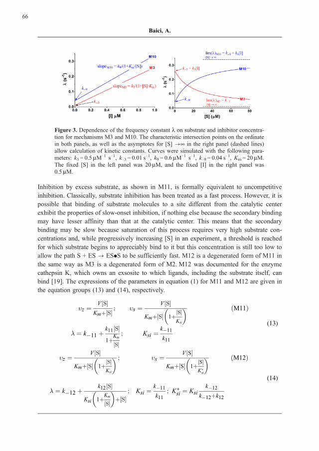
Figure 3. Dependence of the frequency constant l on substrate and inhibitor concentra-

tion for mechanisms M3 and M10. The characteristic intersection points on the ordinate

in both panels, as well as the asymptotes for [S] ?¥ in the right panel (dashed lines)

allow calculation of kinetic constants. Curves were simulated with the following para-

meters: k3 = 0.5mM71 s71, k73 = 0.01 s71, k9 = 0.6mM71 s71, k79 = 0.04 s71, Km = 20mM.

The fixed [S] in the left panel was 20mM, and the fixed [I] in the right panel was

0.5mM.

Inhibition by excess substrate, as shown in M11, is formally equivalent to uncompetitive

inhibition. Classically, substrate inhibition has been treated as a fast process. However, it is

possible that binding of substrate molecules to a site different from the catalytic center

exhibit the properties of slow-onset inhibition, if nothing else because the secondary binding

may have lesser affinity than that at the catalytic center. This means that the secondary

binding may be slow because saturation of this process requires very high substrate con-

centrations and, while progressively increasing [S] in an experiment, a threshold is reached

for which substrate begins to appreciably bind to it but this concentration is still too low to

allow the path S + ES ? ES.S to be sufficiently fast. M12 is a degenerated form of M11 in

the same way as M3 is a degenerated form of M2. M12 was documented for the enzyme

cathepsin K, which owns an exsosite to which ligands, including the substrate itself, can

bind [19]. The expressions of the parameters in equation (1) for M11 and M12 are given in

the equation groups (13) and (14), respectively.

�z ¼V S½ �

Kmþ S½ �; �s ¼

V S½ �

Kmþ S½ � 1þS½ �Ksi

� � ðM11Þ

� ¼ k�11 þk11 S½ �

1þKm

S½ �

; Ksi ¼k�11k11

(13)

�z ¼V S½ �

Kmþ S½ � 1þS½ �Ksi

� � ; �s ¼V S½ �

Kmþ S½ � 1þS½ �K�si

� � ðM12Þ

� ¼ k�12 þk12 S½ �

Ksi 1þKm

S½ �

� �þ S½ �

; Ksi ¼k�11k11

; K�si ¼ Ksik�12

k�12þk12

(14)

66

Baici, A.

Other mechanisms for slow-onset inhibition besides those listed in Scheme 1 are not shown

here. These are likely to occur in practice but not all of them can be unambiguously

identified if not supported by adequate and sufficiently precise data.

The tight-binding condition was not treated in this section devoted to the use of analytical

solutions of differential equations. Indeed, tight-binding represents just an experimental

issue, not an intrinsic property of the mechanisms. Furthermore, an analytical, integrated

rate equation that takes into account inhibitor depletion can be derived for M3 but not for

M2 [3], while for the other mechanisms in Scheme 1 this point was not explicitly addressed

in the literature. Although this derivation is possible for some systems, the necessary

assumptions are too restrictive to be useful in practical situations. Alternatively, numerical

integration methods can be used in place of non-linear regression. For this purpose, a system

of dedicated differential equations can easily be written for each one of the mechanisms in

Scheme 1 and any other mechanism of this type. This labor is even superfluous when using

modern software [10, 11]. The issue is that several models must be applied until the best one

is found but this may be a tedious and time-consuming approach. As far as the pre-steady-

state of progress curves consist of a single exponential, i. e. as long as equation (2) fits data

better than equation (3), the identification of the appropriate model for numerical integration

is possible by preliminary analysis with the diagnostic criteria outlined above using

analytical solutions. Analyzing the parameter dependence on [I] and [S] will give hints as

to which mechanism comes closer to that described by the experiment, no matter if too much

substrate is turned over during the observation time and if plotting parameters against [I]tinstead of [I] will produce bias in the values of the kinetic constants. These can be used later

as initial guesses for refinement by numerical integration once the appropriate model has

been identified.

Enzyme Inactivation

Modifiers can react with elements of the catalytic center of enzymes forming covalent bonds

that result in enzyme inactivation. Common mechanisms observed experimentally for this

category of modifiers are listed in Scheme 2 (M13 – M18), where the symbol E-I distin-

guishes at a glance inactivation from reversible inhibition. Typically, E-I covalent bonds are

formed slowly and reactions can require minutes to hours to proceed to completeness

depending on the characteristic constants of the system and reactant concentrations. For

M13 and M14 the integrated rate equation is (15) and the parameters are given in the

equation groups (16) and (17):

P½ � ¼�z

�1� e��t� �

þ d, (15)

67


�z ¼V S½ �

Km 1þI½ �Ki

� �þ S½ �

; � ¼k4 I½ �

Ki 1þS½ �Km

� �þ I½ �

; Ki ¼k�3k3:

ðM13Þ(16)

�z ¼ �0 ¼V S½ �

Kmþ S½ �; � ¼

k3 I½ �

1þS½ �Km

ðM14Þ (17)

Equation (15) differs from (1) for the absence of the term vs because k74 and k73 equal zero

in M13 and M14, respectively. The diagnosis of these mechanisms is generally easy because

a steady-state is absent in the progress curves (the single exponent levels off to a line parallel

to the time axis for increasing time) and because plots of l versus [I] intersect the ordinate at

zero after any correction for the term d in equation (15). In general however, this last

criterion should not be taken as a demonstration of irreversibility because small values of

k74 and k73 in mechanisms M2, M3 and others, particularly in presence of experimental

scatter, can render impossible the distinction of a small value of the ordinate intercept from

zero.

Scheme 2.Mechanisms of enzyme inactivation. Labeling as M13 – M18 continues the

list of Scheme 1 and numbering of kinetic constants reproduces similar paths for the

reversible counterparts in Scheme 1. E = enzyme, S = substrate, P = product, I = inacti-

vator. E – I denotes a covalent bond between enzyme and inactivator.

Equation (15) is invalid for the temporary inactivation mechanisms M15 and M16 because

the recycled free enzyme can again combine with substrate and inactivator. It is assumed that

the enzymatically transformed inactivator, I*, has lost any affinity for the enzyme. The

appropriate equation is (18), which contains the term v¥ for the velocity ‘at the end’ of

the exponential phase, i. e. t =¥ in e7lt [20]:

P½ � ¼ �1t þ�z��1

�1� e��t� �

þ d: (18)

68

Baici, A.

The velocity term v¥ resembles vs in equation (1) and progress curves have the same shape

as in Figure 1b, which give the impression of a reversible mechanism. Without knowledge

of the temporary character of the inactivation from chemical or other information, an

impulsive diagnosis of such progress curves would suggest either M2 or M3 as candidate

mechanisms. This is evidenced from the expressions of l in equation groups (19) and (20),

which are formally identical to (4) and (5), respectively.

�z ¼V S½ �

Km 1þI½ �Ki

� �þ S½ �

; �1 ¼V S½ �

Km 1þI½ �Ki

1þk4

k5

� �� þ S½ �

ðM15Þ

� ¼ k5 þk4 I½ �

Ki 1þS½ �Km

� �þ I½ �

; Ki ¼k�3k3

(19)

�z ¼ �0 ¼V S½ �

Kmþ S½ �; �1 ¼

V S½ �

Km 1þk3

k5I½ �

� �þ S½ �

ðM16Þ

� ¼ k5 þk3 I½ �

1þS½ �Km

(20)

Mechanisms M15 and M16 are different from mechanism-based (suicide) inhibition, which

is not treated here. A way for discriminating kinetically M15/M16 from M2/M3 is to run

experiments with enzyme and inactivator preincubated for various times, preferentially with

low inactivator concentrations, and to start reactions by adding substrate. Provided the

enzyme is stable during the measuring time, mechanisms M15 and M16 will show pre-

incubation time-dependent regain of enzyme activity until reaching the rate v0 after complete

transformation of all added inactivator to the inert species I*. This cannot happen with

mechanisms M2 and M3 but still the possibility of having to do with the reversible tempor-

ary mechanisms M4 and M5 cannot be ruled out, and here we have reached an end point in

which enzyme kinetics must seek help from other methods for analyzing the fate of the

inactivator after having been in contact with the enzyme. Examples are known from many

published studies, such as a large screening of phosphadecalin derivatives as inactivators of

acetylcholinesterase [20, 21], in which kinetic measurements were supported by NMR

spectroscopy (see [20] and references therein).

The last two inactivation mechanisms in Scheme 2, M17 and M18, apply to unstable

inactivators, to which a meticulous theoretical work has been dedicated [22]. The instability

of some compounds in aqueous solution is often due to hydrolysis that leads to chemically

transformed, inert species (I’ in Scheme 2), which may represent a limitation for their

practical use. Progress curves for M17 and M18 resemble those for reversible inhibition

or temporary inactivation, i. e. they consist of an exponential burst followed by a linear

69


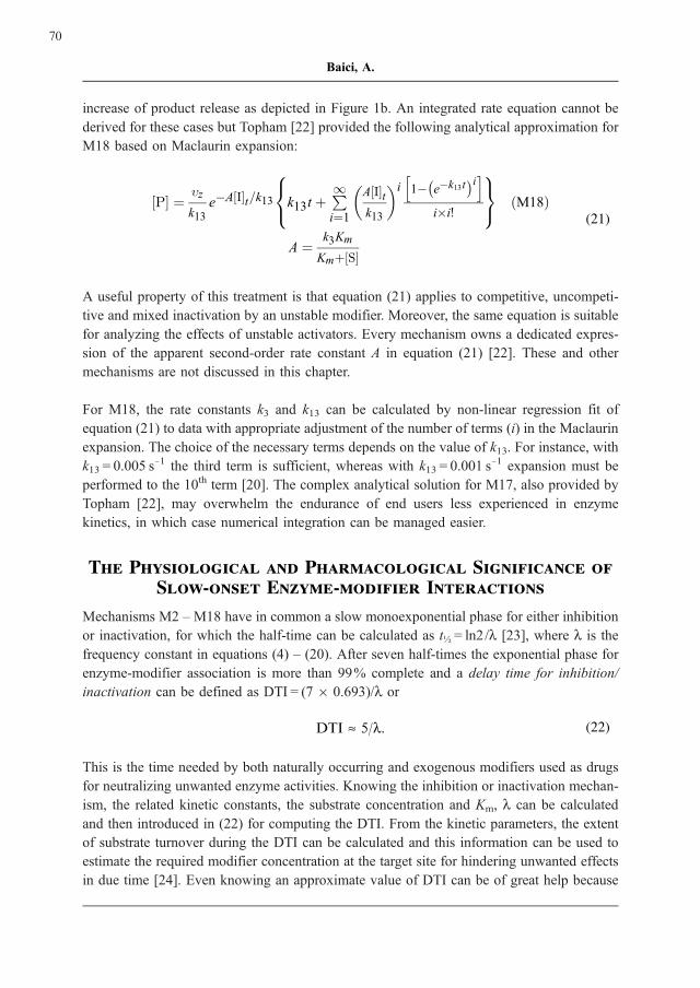
increase of product release as depicted in Figure 1b. An integrated rate equation cannot be

derived for these cases but Topham [22] provided the following analytical approximation for

M18 based on Maclaurin expansion:

P½ � ¼�z

k13e�A I½ �t=k13 k13t þ

P1i¼1

A I½ �tk13

� �i 1� e�k13t� ih i

i�i!

8<:

9=; ðM18Þ

A ¼k3Km

Kmþ S½ �

(21)

A useful property of this treatment is that equation (21) applies to competitive, uncompeti-

tive and mixed inactivation by an unstable modifier. Moreover, the same equation is suitable

for analyzing the effects of unstable activators. Every mechanism owns a dedicated expres-

sion of the apparent second-order rate constant A in equation (21) [22]. These and other

mechanisms are not discussed in this chapter.

For M18, the rate constants k3 and k13 can be calculated by non-linear regression fit of

equation (21) to data with appropriate adjustment of the number of terms (i) in the Maclaurin

expansion. The choice of the necessary terms depends on the value of k13. For instance, with

k13 = 0.005 s71 the third term is sufficient, whereas with k13 = 0.001 s71 expansion must be

performed to the 10th term [20]. The complex analytical solution for M17, also provided by

Topham [22], may overwhelm the endurance of end users less experienced in enzyme

kinetics, in which case numerical integration can be managed easier.

The Physiological and Pharmacological Significance of

Slow-onset Enzyme-modifier Interactions

Mechanisms M2 – M18 have in common a slow monoexponential phase for either inhibition

or inactivation, for which the half-time can be calculated as t½ = ln2/l [23], where l is the

frequency constant in equations (4) – (20). After seven half-times the exponential phase for

enzyme-modifier association is more than 99% complete and a delay time for inhibition/

inactivation can be defined as DTI = (76 0.693)/l or

DTI » 5/l. (22)

This is the time needed by both naturally occurring and exogenous modifiers used as drugs

for neutralizing unwanted enzyme activities. Knowing the inhibition or inactivation mechan-

ism, the related kinetic constants, the substrate concentration and Km, l can be calculated

and then introduced in (22) for computing the DTI. From the kinetic parameters, the extent

of substrate turnover during the DTI can be calculated and this information can be used to

estimate the required modifier concentration at the target site for hindering unwanted effects

in due time [24]. Even knowing an approximate value of DTI can be of great help because

70

Baici, A.

the successful use of enzyme modifiers as drugs depends on modifier bioavailability, con-

centration at the target site and mechanism of inhibition/inactivation. Specifically, if depends

linearly on [I], DTI can be made as short as the modifier concentration can be increased

because DTI? 0 for [I] ?¥. However, if the dependence of l on [I] is hyperbolic, DTI

cannot be shortened below a given threshold because DTI will level off to a plateau even

increasing [I] to infinity. Thus, for a modifier operating with mechanism M2, DTI? 5/(k74 +

k4) for [I] ?¥ and the success in the practical use of this modifier will depend on the values

of k74 and k4.

These simple considerations emphasize that every effort put in determining mechanisms of

action and kinetic parameters for slow-onset enzyme modification as accurately as possible

is not an academic exercise. On the contrary, this knowledge is indispensable for predicting

the physiological and pharmacological significance of the modifiers and can help in the

chemical design of new drugs.

References

[1] Frieden, C. (1970) Kinetic aspects of regulation of metabolic processes. The hystere-

tic enzyme concept. J. Biol. Chem. 245:5788 – 5799.

[2] Cha, S. (1975) Tight-binding inhibitors – I. Kinetic behavior [Erratum: Biochem.

Pharmacol. 25: 1561, 1976]. Biochem. Pharmacol. 24:2177 – 2185.

doi: http://dx.doi.org/10.1016/0006-2952(75)90050-7.

[3] Cha, S. (1976) Tight-binding inhibitors – III. A new approach for the determination

of competition between tight-binding inhibitors and substrates. Inhibition of adeno-

sine deaminase by coformycin. Biochem. Pharmacol. 25:2695 – 2702.


[4] Cha, S. (1980) Tight-binding inhibitors – VII. Extended interpretation of the rate

equation. Experimental designs and statistical methods. Biochem. Pharmacol.

29:1779 – 1789.


[5] Morrison, J.F. (1982) The slow-binding and slow, tight-binding inhibition of enzyme-

catalysed reactions. Trends Biochem. Sci. 7:102 – 105.

doi: http://dx.doi.org/10.1016/0968-0004(82)90157-8,

[6] Morrison, J.F., and Stone, S.R. (1985) Approaches to the study and analysis of the

inhibition of enzymes by slow- and tight-binding inhibitors. Comments Mol. Cell.

Biophys. 2:347 – 368.

[7] Morrison, J.F., and Walsh, C.T. (1988) The behavior and significance of slow-binding

inhibitors. Adv. Enzymol. Relat. Areas Mol. Biol. 61:201 – 301.

71


http://dx.doi.org/10.1016/0006-2952(75)90050-7

http://dx.doi.org/10.1016/0006-2952(76)90259-8

http://dx.doi.org/10.1016/0006-2952(80)90140-9

http://dx.doi.org/10.1016/0968-0004(82)90157-8

[8] Hijazi, N.H., and Laidler, K.J. (1973) Transient-phase and steady-state kinetics for

enzyme activation. Can. J. Biochem. 51:806 – 814.

doi: http://dx.doi.org/10.1139/o73-100.

[9] Neet, K.E., Ohning, G.V., and Woodruff, N.R. (1984) Hysteretic enzymes, slow

inhibition, slow activation, and slow membrane binding. In Dynamics of biochemical

systems, J. Ricard, and A. Cornish-Bowden, eds. (New York, Plenum Press), pp. 3 –

28.

[10] Johnson, K.A., Simpson, Z. B., and Blom, T. (2009) FitSpace Explorer: An algorithm

to evaluate multidimensional parameter space in fitting kinetic data. Anal. Biochem.

387:30 – 41.

doi: http://dx.doi.org/10.1016/j.ab.2008.12.025.

[11] Johnson, K.A., Simpson, Z. B., and Blom, T. (2009) Global Kinetic Explorer: A new

computer program for dynamic simulation and fitting of kinetic data. Anal. Biochem.

387:20 – 29.

doi: http://dx.doi.org/10.1016/j.ab.2008.12.024.

[12] Walmsley, A.R., and Bagshaw, C.R. (1989) Logarithmic timebase for stopped-flow

data acquisition and analysis. Anal. Biochem. 176:313 – 318.


[13] Meh, P., Pavsic, M., Turk, V., Baici, A., and Lenarcic, B. (2005) Dual concentration-

dependent activity of thyroglobulin type-1 domain of testican: specific inhibitor and

substrate of cathepsin L. Biol. Chem. 386:75 – 83.

doi: http://dx.doi.org/10.1515/BC.2005.010.

[14] Dunwiddie, C., Thornberry, N.A., Bull, H.G., Sardana, M., Friedman, P.A., Jacobs,

J.W., and Simpson, E. (1989) Antistasin, a leech-derived inhibitor of factor Xa.

Kinetic analysis of enzyme inhibition and identification of the reactive site. J. Biol.

Chem. 264:16694 – 16699.

[15] Duggleby, R.G., Attwood, P.V., Wallace, J.C., and Keech, D.B. (1982) Avidin is a

slow-binding inhibitor of pyruvate carboxylase. Biochemistry 21:3364 – 3370.

doi: http://dx.doi.org/10.1021/bi00257a018.

[16] Baici, A., and Gyger-Marazzi, M. (1982) The slow, tight-binding inhibition of cathe-

psin B by leupeptin. A hysteretic effect. Eur. J. Biochem. 129:33 – 41.

doi: http://dx.doi.org/10.1111/j.1432-1033.1982.tb07017.x.

[17] Schultz, R.M., Varma-Nelson, P., Ortiz, R., Kozlowski, K.A., Orawski, A.T., Pagast,

P., and Frankfater, A. (1989) Active and inactive forms of the transition-state analog

protease inhibitor leupeptin: explanation of the observed slow binding of leupeptin to

cathepsin B and papain. J. Biol. Chem. 264:1497 – 1507.

72

Baici, A.

http://dx.doi.org/10.1016/0003-2697(89)90315-1

[18] Sivaraman, S., Zwahlen, J., Bell, A.F., Hedstrom, L., and Tonge, P.J. (2003) Struc-

ture-activity studies of the inhibition of FabI, the enoyl reductase from Escherichia

coli, by triclosan: kinetic analysis of mutant FabIs. Biochemistry 42:4406 – 4413.

doi: http://dx.doi.org/10.1021/bi0300229.

[19] Novinec, M., Kovacic, L., Lenarcic, B., and Baici, A. (2010) Conformational flex-

ibility and allosteric regulation of cathepsin K. Biochem. J. 429:379 – 389.

doi: http://dx.doi.org/10.1042/BJ20100337.

[20] Baici, A., Schenker, P., Wachter, M., and Ruedi, P. (2009) 3-Fluoro-2,4-dioxa-3-

phosphadecalins as inhibitors of acetylcholinesterase. A reappraisal of kinetic me-

chanisms and diagnostic methods. Chem. Biodivers. 6:261 – 282.

doi: http://dx.doi.org/10.1002/cbdv.200800334.

[21] Wachter, M., and Ruedi, P. (2009) Synthesis and characterization of the enantiomeri-

cally pure cis- and trans-2,4-dioxa-3-fluoro-3-phosphadecalins as inhibitors of

acetylcholinesterase. Chem. Biodivers. 6:283 – 294.

doi: http://dx.doi.org/10.1002/cbdv.200800335.

[22] Topham, C.M. (1990) A generalized theoretical treatment of the kinetics of an

enzyme-catalysed reaction in the presence of an unstable irreversible modifier.

J. Theor. Biol. 145:547 – 572.

doi: http://dx.doi.org/10.1016/S0022-5193(05)80488-6.

[23] Baici, A. (1988) Criteria for the choice of inhibitors of extracellular matrix-degrading

endopeptidases. In The control of tissue damage, A.M. Glauert, ed. (Amsterdam,

Elsevier), pp. 243 – 258.

[24] Baici, A. (1998) Inhibition of extracellular matrix-degrading endopeptidases:

Problems, comments, and hypotheses. Biol. Chem. 379:1007 – 1018.

73


http://dx.doi.org/10.1016/S0022-5193(05)80488-6

slow-onset enzyme inhibition and inactivationslow-onset enzyme inhibition and inactivation antonio...

Documents