SMALL-SCALE MORPHODYNAMICS OF MAINTAINED AND UNMAINTAINED

BEACHES ON MUSTANG ISLAND, TEXAS

A Thesis

by

MELANIE A. GINGRAS

BA, University of Delaware, 2013

Submitted in Partial Fulfillment of the Requirements for the Degree of

MASTER OF SCIENCE

in

COASTAL AND MARINE SYSTEM SCIENCE

Texas A&M University-Corpus Christi

Corpus Christi, Texas

May 2017

*This is only for degrees previously earned! Please do not include your major

with the degree name, and list the degree simply as BA, BS, MA, etc. For

example: BS, University Name, Year

MS, University Name, Year *International Students must include the name of the country between the school and

the date the degree was received, if it was received outside of the US.

*Delete this box before typing in your information.

© Melanie Ann Gingras

All Rights Reserved

May 2017

SMALL-SCALE MORPHODYNAMICS OF MAINTAINED AND UNMAINTAINED

BEACHES ON MUSTANG ISLAND, TEXAS

A Thesis

by

MELANIE A. GINGRAS

This thesis meets the standards for scope and quality of

Texas A&M University-Corpus Christi and is hereby approved.

James C. Gibeaut, PhD

Chair

Michael Starek, PhD

Committee Member

Philippe Tissot, PhD

Committee Member

May 2017

v

ABSTRACT

In the State of Texas, the public is guaranteed free and unrestricted access to Gulf of

Mexico beaches from the mean low tide line to the vegetation line. This access includes

vehicular traffic and provides for grooming to create a driving lane which is both costly and

unnatural so the study of its effects on beach morphology are important to city planners, local

taxpayers, and beachgoers alike. Therefore, the purpose of this study is to assess the impacts of

beach maintenance practices on the backbeach with the intent of determining maintenance

practices that foster the healthiest morphology while providing unrestricted access.

Two Mustang Island beach sites were chosen for their environmental similarities, but

maintenance differences; one site was frequently maintained and the other site was completely

unmaintained. The sites were scanned during peak maintenance activity using a terrestrial laser

scanner (TLS), were ground-truthed, registered, and georeferenced using a Real-Time Kinematic

(RTK) GPS, and were analyzed in ArcGIS to determine how surface elevations and vegetation

were affected by maintenance.

The Digital Surface Model (DSM) for the maintained site showed a distinctly scarped

profile, sparse vegetation, a vast backbeach driving lane, and little-to-no coppice mounds while

the DSM for the unmaintained site showed a well-developed and gently sloping coppice area

with dense vegetation and a narrow backbeach driving lane. From July to October, the entire

unmaintained site remained stable with small gains in sediment consistent with expected summer

onshore sediment transport while the maintained site experienced losses in the driving lane area

from scraping and large gains in the coppice area from driving lane sand pushed against the dune

toe during maintenance.

vi

Although short in duration, this study implied that maintenance practices could be

improved by maintaining a narrower driving lane. This would promote embryo dune

advancement and vegetation growth for a more dissipative backbeach profile and a more stable

foredune which would better insulate landward developed areas from storm-generated washover

flooding. Finally, the residual comparative analysis between Real-Time Kinematic (RTK) GPS

measurements and the raster products showed high levels of accuracy suggesting promise for

similar future studies using this methodology.

vii

DEDICATION

To my parents who have always been excellent role models and always provided me with

unconditional love and support. Without my mother, Dr. Sally A. Emr, her 23 chromosomes,

unyielding support, fierce passion for education, and firm push to always improve, and my father,

Steven P. Gingras, his 23 chromosomes, logical and analytical excellence, kind example, and

advice, I would not be here. Thank you mom and padre.

Also, to the beach that inspired this project and that has always filled me with a sense of

wonder, sanctuary, and frisson.

viii

ACKNOWLEDGMENTS

I would like to gratefully acknowledge Texas A&M University in Corpus Christi for

affording me the opportunity to pursue a master’s degree in Coastal and Marine System Science

and the various people who have supported me in this endeavor. First, I would like to acknowledge

my advisor and Graduate Committee Chairman, Dr. James C. Gibeaut, Endowed Chair of

Geospatial Sciences at the Harte Research Institute for Gulf of Mexico Studies, for imparting me

with important resources and knowledge of coastal geology without which this thesis would not

have been possible. Next, I would like to recognize the contributions of my committee members

Dr. Michael Starek, who inspired me to pursue a thesis project in the geospatial sciences and

graciously allowed me to borrow his Terrestrial Laser Scanner on several occasions to complete

my field work, and Dr. Philippe Tissot for his mentorship and for allowing me access to his lab

computers, his scientific enthusiasm, his statistical prowess, and his enlightening views on science,

education, and the world. I also would like to humbly thank the NOAA ECSC and the Harte

Research Institute for funding my work and providing valuable traveling and networking

opportunities along the way. Finally, I would like to recognize the contributions of my family,

friends, and coworkers who supported me throughout my graduate school journey. Specifically, I

would like to recognize some of these people by name: Dr. Sally A. Emr, my mother, Steven P.

Gingras, my father, Bryan Gillis, my boyfriend and rock, Melinda Martinez, Luz Lumb, Rachel

Edwards, and Alistair Lord, my coworkers and friends, and Lily Jo Cash, my deaf dog.

ix

TABLE OF CONTENTS

CONTENTS PAGE

ABSTRACT .................................................................................................................................... v

DEDICATION .............................................................................................................................. vii

ACKNOWLEDGMENTS ........................................................................................................... viii

TABLE OF CONTENTS ............................................................................................................... ix

LIST OF FIGURES ....................................................................................................................... xi

LIST OF TABLES ....................................................................................................................... xvi

CHAPTER I: INTRODUCTION .................................................................................................... 1

Beach Maintenance in the State of Texas ................................................................................... 1

Impacts of Beach Maintenance ................................................................................................... 3

Morphodynamics of Mustang Island ........................................................................................... 4

Morphological Features and Dune Succession on Mustang Island ........................................... 12

CHAPTER II: METHODS ........................................................................................................... 16

Field Collection ......................................................................................................................... 20

Pre- and Post-Processing ........................................................................................................... 22

RiSCAN Pro.......................................................................................................................... 22

ArcGIS .................................................................................................................................. 25

CHAPTER III: RESULTS ............................................................................................................ 27

Measurement Uncertainty ......................................................................................................... 46

CHAPTER IV: DISCUSSION ..................................................................................................... 53

Vegetation ................................................................................................................................. 53

Spatial and Temporal Trends .................................................................................................... 54

Dune Advancement ................................................................................................................... 57

x

Method Comparison .................................................................................................................. 59

CHAPTER V: CONCLUSION..................................................................................................... 61

REFERENCES ............................................................................................................................. 64

xi

LIST OF FIGURES

FIGURES PAGE

Figure 1: State of Texas with approximate study area outlined…………………………………...1

Figure 2: Map of study area with maintained and unmaintained study sites marked……………..2

Figure 3: Illustration of location of convergence and direction of currents north of 27⁰N and

south of 27⁰N as discussed in the text………………………………………………………….....6

Figure 4: Illustration of a dissipative coast and its features as described in the text: shore parallel

bars and troughs, gradual gradient, spilling breakers, and a flat/concave beach face………….....7

Figure 5: Wind rose for Mustang Island illustrating the moderate prevailing southeasterlies and

strong northern frontal winds in the study area. Taken from Radosavljevic, 2011…………….....9

Figure 6: Shoreline changes from 2000-2012 along the Texas Coast. Image taken from the Texas

Bureau of Economic Geology Texas Shoreline Change Project webpage………………………10

Figure 7: Morphological features of a Mustang Island beach taken from the University of Texas

at Austin with study area for this study outlined………………………………………………...12

Figure 8: Beach profile of the morphological features in the study area that are present on an

unmaintained beach (top) and a maintained beach (bottom)…………………………………….14

Figure 9: Photograph of Riegl VZ 400 TLS with operational functionality of it portrayed to the

right of scanner…………………………………………………………………………………..18

Figure 10: This image was adapted from Virtanen et al. 2014 to illustrate how the angle and two-

way travel time of laser pulses results in high-resolution point clouds near the scanner and lower

resolution point clouds farther from the scanner………………………………………………...19

Figure 11: Panorama photograph of field set up for the beach scan position at the maintained

site………………………………………………………………………………………………..20

xii

Figure 12: Field map illustrating the relative positions of the targets to the scan positions within

the field site and superimposed on basemap imagery from 2008………………………………..21

Figure 13: Two scan position point clouds as they appear in RiSCAN Pro. The scans depict the

same study site but are in are in their SOCS before merging into a PRCS using tie points to

merge the scans…………………………………………………………………………………..22

Figure 14: Two scans after being merged into a PRCS. Notice the coast does not trend northeast

to southwest as it would be if it were georeferenced in the global coordinate system…………..22

Figure 15: Merged and georeferenced scans before man-made objects (circled in red) were

removed………………………………………………………………………………………….23

Figure 16: Same Scan as Figure 15 but man-made objects have been removed………………...23

Figure 17: Maintained site photograph illustrating the locations of the two polygons, driving lane

and coppice area………………………………………………………………………………….25

Figure 18: Coppice Area and Driving Area polygons overlaid on 2008 imagery of the two

sites………………………………………………………………………………………………25

Figure 19: Bird’s eye view of DSMs of maintained (top right) from the berm to the foredune

ridge and bird’s eye view of unmaintained sites (top left) from the wet dry line to the foredune

ridge in NAD83 UTM Zone 14 (horizontal) and NAVD88 (vertical) obtained on July 22, 2016.

Oblique images looking alongshore of the July DSM for the unmaintained site (bottom left) and

maintained site (bottom right) Note: Differences in foredune slope, width of driving lanes, and

vegetation…………………………………………………………….…………………………..28

Figure 20: Bird's eye view of the DSMs for the scans conducted on July 22, 2016. Horizontal

coordinates are in NAD83 UTM Zone 14 horizontal and elevations are in NAVD88……….....29

xiii

Figure 21: Bird's eye view of the DSMs for the scans conducted on August 10, 2016. Horizontal

coordinates are in NAD83 UTM Zone 14 horizontal and elevations are in NAVD88.………….30

Figure 22: Bird's eye view of the DSMs for the scans conducted on October 3, 2016. Horizontal

coordinates are in NAD83 UTM Zone 14 horizontal and elevations are in NAVD88.………….31

Figure 23: Change DSMs showing the change in elevation from July to August. Areas that are

red experienced erosion while areas that are blue experienced accretion……………………….32

Figure 24: Change DSMs showing the change in elevation from August to October. Areas that

are red experienced erosion while areas that are blue experienced accretion…………..……….33

Figure 25: Change DSMs showing the change in elevation from July to October. Areas that are

red experienced erosion while areas that are blue experienced accretion……………………….34

Figure 26: Transect lines generated using the Interpolate Line Tool in ArcGIS. Again, note the

differences in slope and driving lane width. Both profiles come from Transect 4 in July at their

respective sites (see Figures 30 and 32 for Transect locations)………………………………….35

Figure 27: Unmaintained site coppice area looking from the dune towards the Gulf of Mexico.

Notice the dense vegetation in the coppice area in the center of the picture…………………….36

Figure 28: Maintained site coppice area looking from the dune towards the Gulf of Mexico.

Notice the sparse vegetation in the coppice area in the center of the picture……………………36

Figure 29: The black line outlines the dune mask polygon used to calculate the volume of sand

accreted at the base of the dune from July to October…………………………………………...37

Figure 30: DSM of the maintained site for July indicating the locations of the transects drawn

using the Interpolate Line Tool. Colors of transect lines correspond to colors on Figure 31…...40

Figure 31: Graph of Transects 1-8 at the maintained site extracted from the July DSM. Note:

Slope increases from Transect 1 to 8…………………………………………………………….40

xiv

Figure 32: DSM of the unmaintained site for July indicating the locations of the transects drawn

using the Interpolate Line Tool. Colors of the transect lines correspond to colors in Figure

33…………………………………………………………………………………………………41

Figure 33: Graph of Transects 1-8 at the maintained site extracted from the July DSM. Note: No

discernable trend exists from Transect 1 to 8……………………………………………………41

Figure 34: Transect 8 of the maintained site illustrating that accretion continues to occur in

October…………………………………………………………………………………………...42

Figure 35: Transect 8 of the unmaintained site indicated that accretion peaks in August……….42

Figure 36: DSMs for maintained and unmaintained sites overlaid on satellite base layer imagery

from 2008. Note that the dune toe has advanced since 2008 at both locations but more and

consistently at the unmaintained location………………………………………………………..46

Figure 37: Graph indicating 150 ground truth points from each site paired with their

corresponding DSM elevation points and sorted by elevation…………………………………..47

Figure 38: Graph showing the distribution of residuals for both sites…………………………...47

Figure 39: Elevation differences for RTK GPS elevations and DSM elevations for the maintained

site………………………………………………………………………………………………..48

Figure 40: Distribution of residuals for maintained site…………………………………………48

Figure 41: Elevation differences for RTK GPS elevations and DSM elevations for the

unmaintained site………………………………………………………………………………...49

Figure 42: Distribution of residuals for unmaintained site………………………………………49

Figure 43: Water levels recorded by the Texas Coastal Ocean Observatory Network (TCOON)

station at Bob Hall Pier every six minutes during the study period. Water level rises in the fall.

xv

Spikes in water level indicate thunderstorms and hurricanes, most notable is Hermine in late

August……………………………………………………………………………………………55

xvi

LIST OF TABLES

TABLES PAGE

Table 1: Average point spacings were calculated using the Point File Information Tool in

ArcGIS for original un-clipped and filtered LAS file. The average number of points per square

meter reflects the number of points in the LAS file divided by the area of the shapefile polygon

including both the driving area and coppice area. ........................................................................ 27

Table 2: Changes in surface elevations for maintained coppice area, maintained driving area,

maintained study area, unmaintained coppice area, unmaintained driving area, and unmaintained

study area. ..................................................................................................................................... 38

Table 3: Widths of the driving areas for each transect compared to the corresponding total width

of that transect. Elevation 1.2m was used to distinguish a boundary between the coppice area and

driving area at both sites so all width reported for the driving area are consistently below 1.2 m.

....................................................................................................................................................... 44

Table 4: Widths of the coppice areas for each transect compared to the corresponding total width

of that transect. Elevation 1.2 m was used to distinguish a boundary between the coppice area

and driving area at both sites so all widths reported for width of coppice area are consistently

above 1.2 m. .................................................................................................................................. 44

Table 5: Slopes of the dune profiles at each site calculated by dividing the difference in the

highest profile elevation and 1.2 m by the distance in transect length between the highest

elevation and the last landward elevation of 1.2 m. ...................................................................... 45

Table 6: Summary of residuals and RMSEs for the method comparison. DSM Interpolated

Elevation was subtracted from RTK Elevation to produce residual. ............................................ 52

xvii

Table 7: Average differences and RMSEs for coppice areas, above 1.2 m in elevation, and

driving areas, below 1.2 m elevation, at the maintained and unmaintained sites. DSM

Interpolated Elevation was subtracted from RTK Elevation to produce residual. ....................... 52

Table 8: Temporal residual and RMSE variations with no discernable trends between scan dates.

DSM Interpolated Elevation was subtracted from RTK Elevation to produce residual. .............. 52

1

CHAPTER I: INTRODUCTION

Beach Maintenance in the State of Texas

The Texas Open

Beaches Act (1959) is a

section of the Texas Natural

Resources Code in the

Texas Constitution and

Statutes that provides for

“free and unrestricted

ingress and egress to and

from beaches bordering the

seaward shore of the Gulf of

Mexico (Figure 1) from the

mean low tide line to the

vegetation line”. According to §61.062 of the Texas Natural Resources Code, it is the

responsibility of the local governments of coastal communities to clean and maintain public

beaches and to promote public access. In a very broad sense, cleaning and maintaining refers to

the removal of any hazards that may pose a threat to public health or safety, and promoting

access often includes creating and maintaining access roads and beach driving lanes. In the study

areas on Mustang Island (Figure 2), beach maintenance is performed by the City of Corpus

Christi and Nueces County. Maintenance in these areas includes (1) beach grooming to remove

noisome Sargassum, (2) scraping and compacting the beach surface from the dune toe to the

wet/dry line to create an artificial driving lane to enhance accessibility, and (3) moving the

Figure 1: State of Texas with approximate study area outlined.

2

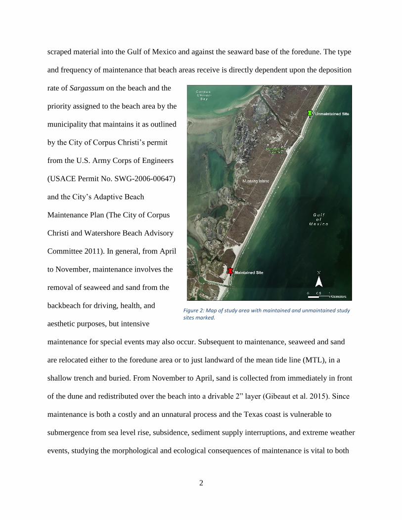
scraped material into the Gulf of Mexico and against the seaward base of the foredune. The type

and frequency of maintenance that beach areas receive is directly dependent upon the deposition

rate of Sargassum on the beach and the

priority assigned to the beach area by the

municipality that maintains it as outlined

by the City of Corpus Christi’s permit

from the U.S. Army Corps of Engineers

(USACE Permit No. SWG-2006-00647)

and the City’s Adaptive Beach

Maintenance Plan (The City of Corpus

Christi and Watershore Beach Advisory

Committee 2011). In general, from April

to November, maintenance involves the

removal of seaweed and sand from the

backbeach for driving, health, and

aesthetic purposes, but intensive

maintenance for special events may also occur. Subsequent to maintenance, seaweed and sand

are relocated either to the foredune area or to just landward of the mean tide line (MTL), in a

shallow trench and buried. From November to April, sand is collected from immediately in front

of the dune and redistributed over the beach into a drivable 2” layer (Gibeaut et al. 2015). Since

maintenance is both a costly and an unnatural process and the Texas coast is vulnerable to

submergence from sea level rise, subsidence, sediment supply interruptions, and extreme weather

events, studying the morphological and ecological consequences of maintenance is vital to both

Figure 2: Map of study area with maintained and unmaintained study sites marked.

3

city planning and conservation efforts. Therefore, the purpose of this study is to assess the

impacts of beach maintenance practices on the backbeach with the intent of determining

maintenance practices that foster the healthiest morphology while providing unrestricted access

to the public.

Impacts of Beach Maintenance

Studies are ongoing since there is a definite paucity of data regarding the possible

repercussions of beach management but several previous studies of maintained and unmaintained

beaches have emerged bearing controversial results regarding changes to animal communities,

vegetation, and beach morphology as direct consequences of maintenance practices. A study

found significant losses of shorebird prey that was linked to changes in bird community structure

on groomed beaches in California (Dugan, Hubbard, McCrary, & Pierson, 2003). A more recent

study by Smith, Harrison, and Rowland (2011) in Australia found shorebird prey to be robust

and found no lasting difference in infauna or bird community structure on groomed versus

ungroomed beaches, which corroborated the findings of two Texas studies: one conducted in

1997 by the Padre Island National Seashore (Engelhard & Withers, 1997) and one conducted by

HDR Engineering Inc. in 2013. A study in 2010 by Dugan and Hubbard found that vegetation

on groomed beaches is sparser and less diverse but this may not be a direct product of grooming

but rather the secondary consequences suffered by a well-traveled beach (Grunewald &

Schubert, 2007; Houser, Labude, Haider, & Weymer, 2013; McAtee & Drawe, 1981). However,

some studies indicate that grooming and beach driving may directly impact sediment transport

by enhancing the amount of unconsolidated sand, which may influence backbeach and foredune

elevation, bury vegetation, and increase the number of blowouts produced during extreme events

(Lancaster & Baas 1998; Nordstrom, Jackson, & Korotky, 2011; Houser et al. 2013; Nordstrom,

4

Gamper, Fontolan, Bezzi, & Jackson, 2009; Hesp 2002; Conaway & Wells 2005; Dugan &

Hubbard 2010). A study conducted in 2013 scanned the surfaces of beaches in Maryland and

Texas and found that beach driving lowered overall dune elevation and reduced vegetation

(Houser et al., 2013). The most recent investigation in the study area was completed in 2015 by

the Harte Research Institute for Gulf of Mexico Studies under the Coastal Erosion and Planning

Response Act (CEPRA). It used quarterly dune surveys from September 2008-March 2015 to

monitor seasonal beach changes, which remained generally unchanged over the years. Airborne

LiDAR was used to generate digital surface models (DSMs) that were used to compute

volumetric changes in dunes from 2005-2010 and were determined to be inconclusive due to

confounding jetty influence. Finally, two vegetation surveys were performed from December

2014 to July 2015, which corroborated Dugan and Hubbard’s findings in 2010 that grooming the

beach results in a wider unvegetated sand flat, diminishes both biodiversity and species

abundance of flora and fauna, and enhances sediment transport. The inconclusiveness of the

previous beach management studies and the physical vulnerabilities of the study area necessitate

further study of these maintenance practices to determine what impact, if any, maintenance has

on the morphology of the Texas coast and whether or not there is a way to improve maintenance

practices without infringing upon the public’s right to access the beach.

Morphodynamics of Mustang Island

Mustang Island is a microtidal barrier island that trends northeast to southwest along the

south-central portion of the Texas Gulf Coast. It is bound in the west by Corpus Christi Bay and

Laguna Madre, in the east by the Gulf of Mexico, in the north by Aransas Pass, and in the south

by Packery Channel. Astronomical tides along the Gulf-side of Mustang Island are generally

considered diurnal or mixed with a mean tide range of 31 cm and a diurnal range of 50 cm with a

5

much smaller range in the bay (10-30 cm) the water level of which is more frequently governed

by wind (Montagna, Gibeaut, & Tunnell Jr, 2007; Morton & McGowen, 1980). Climactically,

Corpus Christi, Texas where, Mustang Island is located, is considered semiarid because it lies at

the boundary where precipitation exceeds evaporation to the north and evaporation exceeds

precipitation to the south (Montagna et al., 2007). Precipitation is important for sediment

accretion because moisture anchors sediment and sustains sediment-securing vegetation. From

the northeast to the southwest of the Texas coast, there is a decrease in precipitation,

sedimentation, distribution of wetlands, and subsidence, and an increase in active dunes and

reduced vegetation cover leading to more theoretically stable conditions in the north and

erosional conditions in the south (White, Morton, & Holmes, 2001).

Since the barrier island system emerged approximately 4,000 year BP, as a result of slow

sea level rise and ample sediment supply, it has progressed through three barrier island stages:

accretionary, stable, and erosional. It has been built vertically by the wind, built Gulfward by

marine forces, and built lagoonward by washover deposition (Weise & White, 1980). Mustang

Island lies in a stable portion of the Texas Coast, which due to an ample sediment supply and

wave-dominated processes, has become a high profile barrier meaning that its high dunes block

most material from being transported to the backbarrier environment and Mustang Island is more

stable than its neighbors to the north and south as a result (Morton & McGowen, 1980).

Due to the arcuate shape of the Texas Coast and the prevailing southeasterly winds, Mustang

Island formed in a very sedimentologically stable area just north of a longshore convergence

zone at 27⁰N (Lohse, 1955; Curray, 1960; Morton, 1979). Aside from seasonal and storm

variations in wind patterns, the longshore currents have remained relatively uninterrupted for

thousands of years and as sea level has risen slowly conditions were favorable for the formation

6

of broken sandbars, then spits, and finally a continuous barrier island (Hayes, 1979). Longshore

currents in east Texas typically flow southwest down to 27⁰N (Big Shell Beach), while longshore

currents in south Texas typically flow north up to 27⁰N (Figure 3), although, as local prevailing

winds shift so does the direction of the current and the location of convergence (Curray, 1960;

Behrens, Watson, & Mason, 1977; McGowen, Garner, &Wilkinson, 1977). Prevailing

southeastern winds in Corpus Christi typically produce a north-flowing current while northerly

front systems tend to produce south flowing currents.

Figure 3: Illustration of location of convergence and direction of currents north of 27⁰N and south of 27⁰N as discussed in the text.

7

The Texas Coast can be classified as a passive trailing-edge marginal sea coast, which

means that it has few-to no instances of tectonic activity, a wide continental shelf, mature

drainage and erosional features, and low-lying landforms (Inman & Nordstrom, 1971). The

stability of a passive marginal sea coast, abundant sediment supply, vast continental shelf to store

the sediment, low to moderate wave energy, and minimal fluvial and tidal influences has enabled

Mustang Island to persist for thousands of years and retain its wave-dominated shape (Hayes,

1979). There is little riverine influence so deltaic digitate lobes prograding into the Gulf are

absent and its small tidal range and tidal prism inhibit the formation of ebb tidal deltas and tide-

parallel sand bars. Instead, Mustang Island features a straight uninterrupted fine-sand coastline.

The fine-sand originates from ancient and present riverine deposits to the north and south that are

transported alongshore to settle on the shoreface, the broad area seaward of the surf zone

extending to the continental shelf that acts as a sand reservoir, transported either landward to the

beach and upper shoreface or seaward to the lower shoreface or offshore by waves.

Figure 4: Illustration of a dissipative coast and its features as described in the text: shore parallel bars and troughs, gradual gradient, spilling breakers, and a flat/concave beach face.

8

Overall, the modal state of Mustang Island is dissipative (Figure 4). The modal state of a

beach is determined by the most recurrent breaker characteristics and prevailing sediment

characteristics as well as certain depositional forms and hydrodynamic process signatures. The

breaker characteristics most common to Mustang Island are ~1 m high waves at a period of ~5 s

and the prevailing sediment is well-sorted fine sand of which the sediment fall velocity is

approximately 0.7 cm/s. According to Wright and Short (1984), these parameters can be used to

determine the state of the beach by dividing the average breaker height by the average wave

period and sediment fall velocity. The resulting number will determine if the beach is reflective

(less than 1), intermediate (between 1 and 6), or dissipative (greater than 6). With a value of

almost 30 for these average parameter values, Mustang Island is well-within the range for a

dissipative beach. In appearance, Mustang Island also resembles a dissipative beach. It has a

low-sloping and wide beach face consisting of fine sand, a low gradient and wide continental

shelf where an abundance of sediment is stored, and a wide surf zone (300-500 m) containing

three longshore bars where spilling breakers dissipate their energy as they approach the subaerial

beach (Wright & Short, 1984). Usually, waves tend to transport sand onshore but as wind and

wave patterns vary seasonally this does tend to oscillate between a very nourished beach profile

in the summer and a steeper less nourished profile in the winter as the sand that is moved from

the lower shoreface to the beach returns.

The typical summer southeasterly winds blow at moderate speeds between 3 and 9 m/s

producing north-flowing longshore currents and beach-constructive waves while strong winter

northeasterly winds blow at speeds greater than 12 m/s (Figure 5) producing south-flowing

longshore currents and beach-destructive waves (Lohse, 1952; Curray, 1960; Watson, 1971;

Morton, 1979; Morton & McGowen, 1980; Short & Hesp, 1982; Davis & Hayes, 1984;

9

Niedoroda, Swift, Hopkins, & Ma, 1984; Wright & Short, 1984; Wright, Short, & Green, 1985;

Morton, 1988). Summer waves tend to be small in the Gulf with landward net orbital stresses

that tend to entrain sediment from the lower shoreface and transport it to the upper shoreface and

beach during the summer months making the beach gradient even lower. During the winter,

wave heights increase and periods shorten resulting in downwelling and a seaward bottom

current that that transports sediment from the beach and upper shoreface to the lower shoreface

leaving behind a steeper and more scarped beach and steeper nearshore profile. It is also

important to note that

Mustang Island is

storm-dominated

meaning that dramatic

morphological

changes from cyclones

are far greater than

changes exerted on the

morphology by daily

processes and seasonal

variations. During

extreme events a storm

surge ebb can

transport sand so far

offshore that it is lost

from the seasonal sediment budget on the shoreface (Bascom, 1964).

Figure 5: Wind rose for Mustang Island illustrating the moderate prevailing southeasterlies and strong northern frontal winds in the study area. Taken from Radosavljevic, 2011.

10

Although several natural forces are at work eroding the Texas Coast, anthropogenic forces

have begun to outpace natural forces in some areas. Most of the long-term coastal erosion taking

place in Texas is a result of eustatic cycles and relative sea level rise. As a result of these eustatic

changes, pore fluid extraction, and sediment loading, the Texas coast has experienced periods of

growth, stability, and rapid retreat. The dominant process often depends on sediment supply and

antecedent (Pleistocene) topography. The current eustatic cycle began ~120 ka before present but

for the last 2 ka, rapid retreat has been the dominant process brought about by reduced sediment

supply from river deltas, longshore currents, storm impacts, and anthropogenic influences

(Anderson et al., 2014). The relative rates of sea-level rise for Mustang Island most likely fall

somewhere within the range of measured rates from the neighboring tidal-gauge-equipped cities:

Figure 6: Shoreline changes from 2000-2012 along the Texas Coast. Image taken from the Texas Bureau of Economic Geology Texas Shoreline Change Project webpage.

11

Rockport (measured since 1948), Port Mansfield (measured since 1963), and South Padre Island

(measured since 1958); 4.6 mm/yr, 2.05 mm/yr,, and 3.44 mm/yr , respectively (Montagna et al.,

2007). Sea-level rise and vast amounts of sediment, which initially fueled the formation of the

barrier island, now threaten to transgress, force landward, and sink the island. Land subsidence

rates on the south Texas barrier islands are 1 to 5 mm/yr Montagna et al., 2007) and, in general,

areas with thick, rapidly deposited sediment and pore fluid extraction have a higher rate of

compaction and isotactic subsidence. Overall, the erosion rate for the Texas Coast for the last

century has been -1.2 ± 1.3 m/yr while the average the short-term erosion rate (2000-2007) has

been -2.6 m/yr but places like Sargent Beach, Galveston, Port Mansfield, and Surfside have

accelerated long-term erosional rates closer to -4.4 ± 2.2 m/yr and short-term erosional rates

nearing -6.4 m/yr due to largely anthropogenic influences (Paine, Mathew, & Caudle, 2012).

Man-made channels, processes, and structures have interfered with the rate of sea level rise

and the natural transport of sediment resulting local areas of erosion that could weaken the

coast’s resilience during storm events and are the most perceptible influence on Mustang Island.

In Texas, the shipping industry places heavy demands on the creation and maintenance of

shipping channels. Usually when shipping channels are dredged, the dredged material is

deposited offshore and lost to the seasonal sediment budget. Jetties and groins often accompany

shipping channels and are another prime example of interrupted sediment flows because they

interrupt longshore currents and produce uneven erosion of the coast. Jetties and groins have a

highly erosional down-current side and an accretional up-current side so certain portions of the

beach will be much more vulnerable than others and will breech more easily during extreme

events. In Figure 6, most of the areas experiencing erosional changes greater than 4.5 m/yr are at

the locations of manmade jetties and channels.

12

Accordingly, the study sites were selected for their natural and anthropogenic similarities

with the exception of differing maintenance practices. Both study sites were located north (up-

current) side of jetties, permitted driving, and were close enough to one another that the wind and

wave regimes were essentially identical (Figure 2). Thus, the main difference between the two

sites was whether or not the site was bulldozed by the local municipalities to create a driving

lane and it is the impact of beach maintenance on the backbeach that this study seeks to identify.

Figure 7: Morphological features of a Mustang Island beach taken from the University of Texas at Austin with study area for this study outlined.

Morphological Features and Dune Succession on Mustang Island

The beach of Mustang Island is comprised of two zones (Figures 7 and 8): the forebeach,

which dips seaward from the berm crest to the breaker zone, and the backbeach which

encompasses the area from the berm crest to the fore-island dunes (McGowan et al. 1977). The

beach substrate is fine, well-sorted sand, comprised of quartz, feldspar, rock and shell fragments,

and heavy minerals (Bullard, 1942). The backbeach, which is the gently sloping dry sand part of

the beach, can be barren and entirely flat and wind scoured, or it can be covered with coppice

dunes that extend to the fore-island dunes (the seaward most established dune oriented

alongshore). The fore-island dune ridge is a mostly continuous 6-12 meter high wall of coalesced

or multiple dunes of wind-blown sand and vegetation that protect the barrier flat from storm

13

damage (Brown et al., 1976). Behind the foredune ridge is a gently sloping vegetated barrier flat

intermittently broken by stabilized blowout dunes, active blowout dunes, areas of hummocky

small dunes, and stabilized mid-island dunes.

Seaward of the forebeach, the nearshore has three prominent bars that migrate as wave

behavior changes and wave behavior changes as the wind changes. As waves approach the

seaward most bar of the outer breaker zone (Figure 4), the top of the wave outpaces the shoaling

bottom and white water spills over the face. This happens two more times as the swash bore

continues to dissipate energy over the wide surf zone and longshore bars until an attenuated

version of the wave encounters the subaerial beach. In the summer, constructive waves move

sand and longshore bars landward, producing healthy berms, a nourished beach, and an even

more gradual gradient. In the winter, steep and destructive waves erode the beach, scarp berms,

and move sand and longshore bars away from the beach. In the swash zone, small cusps may

form when approaching wave crests are parallel to shore and they can become more pronounced

if parallel wave action is prolonged. More commonly on Mustang Island waves approach the

shore from oblique angles destroying cusps and creating straight coast or introducing asymmetry

to the cusps as sediment is transported along shore to the north during typical wind conditions or

to the south during frontal wind conditions (Ashton, Murray, & Arnoult, 2001).

In this study, beach morphology refers to the form and structure of the backbeach area

from the landward extent of the forebeach to the foredune ridge. The backbeach is often where a

driving lane is maintained from the dune toe to the berm crest. The dune toe is the seaward-most

extent of the foredune and is characterized by a rapid increase in elevation and established

vegetation that is dense and diverse. Seaward of the foredune, there may be small mounds of

sand anchored by pioneer species of vegetation or surf wrack debris or continuous incipient or

14

Figure 8: Beach profile of the morphological features in the study area that are present on an unmaintained beach (top) and a maintained beach (bottom).

embryo dunes that are formed when the mounds coalesce. Over time these pioneer species, often

stoloniferous, provide humus for secondary plant species to thrive and continue to entrap sand.

Depending on the beach width, sediment supply, and winds these incipient foredunes may merge

with or become entirely new foredunes (Hesp, 2002). New foredunes are usually more than a

meter in height and contain organic matter suitable for both stoloniferous vegetation and rhizome

plant species. Wide beaches with ample sand supply and substantial winds to transport the sand

supply provide the greatest potential for forming new foredunes from incipient dunes (Hesp,

2012). Incipient dunes can develop vertically and coalesce seaward of an existing foredune until

they become foredunes, they can migrate inland and join the current foredune, or become

destroyed and redistributed over the beach surface. If wind speeds are high and sediment supply

15

is low, sediment from embryo dunes will likely be redistributed over the beach surface or

migrate landward to join the foredune. If wind speeds are low and sediment supply is great, a

new seaward foredune ridge may develop from the embryo dune.

Often plant species found on foredunes are rhizomatous or stoloniferous and are adept at

capturing sand for vertical development. On Mustang Island, these species include Heterotheca

subaxillaris, Ipomea imperati, Impomea prescaprae, Ipomea stolonifera, Panicum amarum,

Croton capitatus, Amaranthus greggi, Sporobulus viginicus, Uniola paniculata, Sesuviam

portulacastrum, Coccoloba uvifera, and Cakile geniculate. On foredunes where vegetation is

sparse and winds are onshore, there will be fewer opportunities for the wind-entrained sand to be

slowed to settling velocities on the stoss face. The wind tends to accelerate up to the crest

transporting entrained sand higher up the stoss face over the crest and onto the lee slope. When

the foredune is well-vegetated, deposition often takes place near the dune toe or near the base of

the stoss face allowing the dune to prograde if sediment supply is ample (Hesp, 1988). Mustang

Island has an abundant sediment supply, moderate onshore winds, and in the absence of human

interference, dense vegetation so embryo dunes often form, migrate landward, and adjoin the

seaward portion of the foredune creating a slowly prograding foredune.

Sea level can also play an important role in foredune morphology. On beaches where the sea

is transgressing, the stoss slope erodes becoming steeper or scarped as the crest height increases

and the dune retreats landward (Saunders & Davidson-Arnott, 1990; Short & Hesp, 1999). On

Mustang Island, transgression has been slow so this is not yet present but it is likely that in the

future as the rate of sea level rise increases, squeezing of the dunes will be observed. However,

sediment supply and winds are sufficient to produce gradually advancing foredunes at present.

16

CHAPTER II: METHODS

A Terrestrial Laser Scanner (TLS) was used to acquire point clouds at the two sites during

the summer months of 2016 when beach maintenance was at a maximum. Scans were performed

on July, 21st, August11th, and October 3rd and, immediately following the scans, 50 ground

points were collected at each site using an RTK GPS for the purpose of performing a method

comparison of the elevations of the Digital Surface Models (DSMs) derived from the point

clouds of the TLS and the elevations gathered by the RTK GPS ground truth surveys. The point

cloud data from these scans was imported into the Riegl software, RiSCAN Pro, for pre-

processing before ArcGIS was used to post-process the data and render DSMs for analysis.

LiDAR stands for Light Detection and Ranging and is an active sensing technique that

uses laser pulses to gather three dimensional land surface data from an airborne or a terrestrial

platform. This study used a Riegl VZ-400 Terrestrial Laser Scanner to perform the high temporal

and spatial resolution scans required for analysis of beach changes. Although past morphological

change studies have measured individual beach profiles gathered using Emery rods, RTK GPS,

or an electronic total station, this study sought to explore a larger area of the beach in fine detail

to better understand how the beach surface responds to maintenance. This is a significant

improvement over RTK GPS because time would limit the area and number of discrete points

that RTK GPS could collect at a high resolution and accuracy. Additionally, systematic and

random error could be introduced by the sinking of the rover antenna pole into the

unconsolidated coppice dune sediment and compacted driving lane sediment during RTK GPS

measurements. Structure from Motion (SfM) photogrammetry using an aerial platform such as a

UAV was also dismissed as a data collection method due to its reliance on unique feature

matching between overlapping photographs and reduced vertical accuracy relative to TLS. The

17

beach is relatively homogeneous in appearance, which has been shown to result in diminished

point density (Mancini et al., 2013) of the SfM technique and would hinder this study’s ability to

resolve small vertical changes at the magnitudes expected during the short study period. Finally,

airborne LiDAR was not selected for both cost and resolution purposes. The cost of airborne

LiDAR for a 31,614 acre study area to produce a 20 m resolution raster surface was $79,028

according to a 2011 study (Hummel, Hudak, Uebler, Falkowski, & Megown., 2011). This far-

exceeded the funding budget of this study and mapped a larger area than was necessary for the

scope of this study. Additionally, the best resolution reported for airborne data is 15 cm (Greaves

et al., 2016), which would require a more precise and expensive airborne system than used in the

Hummel study, and while 15 cm is excellent for large-area watershed and biomass studies it was

unsuitable for the small-scale morphological changes this study hoped to detect. Additionally,

the positional error budget of airborne LiDAR greatly exceeds that of TLS due to a much larger

illumination footprint, propagation of error from direct georeferencing, IMU misalignment,

reduced point spacing, and other factors. Therefore, it was appropriate to select this TLS system

for data collection because it is capable of 5 mm accuracy, 3 mm precision, and a range of 600 m

at hyperspatial sampling density (sub-cm if needed) allowing observations of slight volumetric

fluctuations in the backbeach, coppice mound area, and the seaward portion of the foredune to be

detected.

As mentioned above, TLSs are a form of ground-based LiDAR (Figure 9) that use lasers to

collect dense point clouds of data, which when processed, are capable of forming DSMs with

sub-centimeter accuracy; however, absolute accuracy of a DSM derived from a single scan will

depend on the level of accuracy in the georeferencing framework utilized (e.g. RTK GPS) and

other factors, such as beam divergence as you move farther away from the scanner. Lasers are

18

coherent, high energy, monochromatic, and highly directional beams of light that penetrate

through air, and reflect off most surfaces making them ideal for collecting range data quickly.

Traditionally, LiDAR systems used a phase difference, time-of-flight, and optical triangulation to

determine the distance between a target and the sensor. However, with the advent of short-pulse

lasers, digitizing and recording the intensity-time profile of the outgoing and returning pulses

became possible, which practically eliminated ambiguities in time-of-flight. Despite these

advances, some error can arise. Multipathing, which is when the laser beam bounces off of

multiple objects before returning to the sensor effectively lengthens the measured travel time and

thus provides a falsely distant point. This, however, was unlikely in this study given the openness

of the study site. Beam divergence, which is a

meager 0.35 mrad for the Riegl scanner (~4

cm diameter footprint at 100 m with a 7 mm

initial pulse diameter), affects the

observations at greater distances from the

sensor as the beam becomes more scattered

and less coherent, creating a less precise point

position due to the larger area the laser

occupies. Beam divergence was also unlikely

to result in large point position errors and all

points more than 200 m from the scanner

were removed prior to analysis to mitigate

this issue.

Figure 9: Photograph of Riegl VZ 400 TLS with operational functionality of it portrayed to the right of scanner

19

The sensor of the Riegl TLS uses a rotating mirror to rapidly emit near infrared laser

pulses and absorb returning laser pulses to generate a point cloud. It accomplishes this by

recording the two-way travel time, azimuth, zenith, range, and intensity of an emitted and

retuned pulse (Figure 10) at a Pulse Repetition Rate of 100 kHz to record thousands of target

distances and intensities each second and converts this information into a point cloud in a

scanner-centered reference frame. A 360⁰ scan can be completed within 5-35 minutes depending

on the desired resolution. The point spacings for this study can be found in Table 1. Although not

utilized for this study, the Riegl VZ400 is equipped with echo digitization to process full

waveforms of the returned laser pulse to distinguish the three dimensions present rather than the

limited 2.5D surface often produced by a single-return system. Laser pulse settings can be

changed to produce dense or sparse point clouds with larger or smaller uncertainties in the final

DSM products. For the purpose of this study, high density point spacing was essential.

Because the recorded centimeter-resolution point cloud was in a scanner-centered

reference frame, a registration method needed to be employed in order to merge and

georeference the point clouds. University NAVSTAR Consortium (UNAVCO) suggests targets

or feature matching, also known as Free Stationing, as the preferred and most accurate method

and thus is the method used in this study. For other applications, other options exist such as (1)

Figure 10: This image was adapted from Virtanen et al. 2014 to illustrate how the angle and two-way travel time of laser pulses results in high-resolution point clouds near the scanner and lower resolution point clouds farther from the scanner.

20

direct georeferencing using the integrated GPS receiver to determine scan position, (2) GNSS

traversing using onboard inclination sensors and automatic acquisition of a well-known remote

target, or (3) backsighting which involves fine scanning of a well-known remote target.

However, because the RTK GPS is much more accurate than the integrated GPS receiver on the

scanner and because the beach is so dynamic that fixing a reliable remote target was not

practicable, on each scan day four 10-cm retro-reflective cylindrical targets were assembled

uniformly throughout each study site and the x, y, and z RTK GPS coordinates were collected

using reference ellipsoid WGS84 and GEOID Model GEOID12B to convert the measurements

into NAD83 UTM Zone 14 (horizontal) and NAVD88 (vertical) for registration and

georeferencing purposes. The RTK GPS receiver acquired differential corrections from the

Western Data Systems (WDS) Virtual Reference Station (VRS) network with reported

accuracies of ±1 cm horizontally and ±2 cm vertically.

Field Collection

As mentioned, the field portion of this study employed Free Stationing to collect and

register scan data. A leveled Seco tripod with a central topo shoe set to 1.5m was used for the

base on which the TLS was secured during the beach scans and four 10-cm cylindrical retro-

reflector targets were fastened to leveled Leica tribrachs atop Seco aluminum tripods and Sokkia

wooden tripods throughout the study sites to provide geodetic control (Figures 11 and 12).

Because the scanner can only generate points on objects that face the laser, data were collected at

two scan positions at each site. One scan position was located near to or on the beach and the

other scan position was located high in the coppice dune area in order to generate points on both

sides of coppice mounds and other beach surface irregularities. For each scan, the rotation or

21

yaw angle of the scanner was set to begin at 0 degrees to finish at 360 degrees. The rotation

angle scanned a full 360 degrees because the scan positions were located in the beach and

coppice dune areas which were

both surrounded by relevant areas

to this study. The pitch of the

mirror was set to oscillate

between -60 degrees (the

minimum allowable by the

scanner) and 78 degrees, which

proved to be optimal for scanning

just to the top of the foredune

ridge. The laser pulses were set to

be emitted at a mirror stepping angle of 0.018 degrees (~0.0003 radians) horizontally and

vertically, which enabled a single scan in long range mode to be completed within 35 minutes.

At this stepping resolution, the average point spacing at a 100 m radial distance from the scanner

is approximately 3 cm. During the scan, ground truth points were gathered using an RTK GPS,

which, as mentioned, has a vertical uncertainty of ±2 cm and horizontal uncertainty of ±1 cm, for

a comparative statistical analysis of accuracy and precision of the elevation collection methods.

At the conclusion of the scan, the retro-reflector targets were identified manually on a field tough

Figure 11: Panorama photograph of field set up for the beach scan position at the maintained site.

Figure 12: Field map illustrating the relative positions of the targets to the scan positions within the field site and superimposed on basemap imagery from 2008.

22

book and were fine scanned to be registered later. Once all of the targets were fine-scanned, the

TLS was relocated to the second scan position and the high-resolution scanning process was

repeated. Once both scans at a location

were completed, 50 ground truth

points were collected using the

Trimble R8 RTK GNSS for later

comparison with interpolated DSM

elevations.

Pre- and Post-Processing

RiSCAN Pro

Once the scans were collected,

pre-processing was completed in

Riegl’s RiSCAN Pro. Initially, each of

the scans was in its own scanner-

centered Scanner’s Own Coordinate

System (SOCS). The SOCS shows

the positions of the scene points

relative to the scanner’s position so

when point clouds from multiple

scan positions at the same site were

viewed together in RiSCAN Pro

(Figure 13), identical objects, such as

the jetty, do not overlap. This is

Figure 13: Two scan position point clouds as they appear in RiSCAN Pro. The scans depict the same study site but are in are in their SOCS before merging into a PRCS using tie points to merge the scans.

Figure 14: Two scans after being merged into a PRCS. Notice the coast does not trend northeast to southwest as it would be if it were georeferenced in the global coordinate system.

23

because the position of the scanner

was different from scan to scan but

the software only recognizes the scan

position of each scan and placed

them in the same location. Once the

software was informed that there

were identical features that should be

made to overlap, tie points, the

scans could be co-registered so that they were properly oriented. This can be seen in Figure 13,

where only scan position two was visible because scan position one was imported first and was

placed in the same location but directly underneath and obscured by scan position two. In

reality, scan position one and scan position two were in different locations (Figure 14) but before

the scans were merged the software was unaware of this. The first step in correcting these

conflicting spatial orientations was to identify the targets (i.e. tie points) in both scans and use

them to merge the scans into a shared Project Coordinate System (PRCS). The software does this

by using a cylindrical shape fitting

algorithm that fixes the target tie

point in the center of the cylinder.

At this point, the scans were not

georeferenced but were co-

registered such that when overlaid

they did show the overlap of

identical features and scan

Figure 15: Merged and georeferenced scans before man-made objects (circled in red) were removed.

Figure 16: Same scan as Figure 15 but man-made objects have been removed.

24

positions were in their correct locations relative to one another. However, until the merged scans

were georeferenced, the coast was not oriented correctly, which would prevent a temporal

analysis in post-processing. Therefore, to georeference the point clouds the RTK x, y, and z

coordinates of the tie points in NAD83 UTM Zone 14 and NAVD88 were imported as a text or

comma delimited file under the Global Coordinate System (GLCS) heading in RiSCAN Pro.

Five centimeters were added to the z coordinates of each target because the antenna position

recorded by the RTK corresponded to the bottom of the 10-cm cylinder so the addition of the

five centimeters ensured that the RTK coordinates represented the point at the center of the

target, which is designated during the target shape fitting process of the software as explained

above. Georeferencing is then based on a weighted least-squares affine transformation (without

scaling) of the four target project coordinates relative to their georeferenced coordinates derived

from the RTK GPS. In this case, each GPS observation had equal weighting due to similar

uncertainties.

Once the scans were georeferenced, the point clouds were prepared for export. Foremost,

all points more than 200 m from the scanner were removed. Next, all man-made objects were

removed from the beach surface since the purpose of the study was to measure morphological

change of the beach surface and not the movement of man-made objects on the beach. Removal

was accomplished using polyline manual selection and deleting unwanted items such as vehicles,

signs, fences, dune walkovers, lifeguard stands, people, posts, refuse bins, and tents. Due to

computational limitations, a 2 cm x 2 cm x 2 cm octree filter was applied. The octree filter

diminished the mm resolution close to the scanner to evenly distribute the elevation points at a

uniform distance of 2 cm between each point throughout the study site while mitigating some of

the small changes that may have occurred between scans. This reduced the large file size

25

precipitated by the high concentration of points next to the scanner while still retaining a near

cm-resolution, albeit more uniform, point cloud. Finally, the merged, georeferenced, and cleaned

scans were exported from RiSCAN Pro as an LAS file and imported into ArcGIS for post-

processing.

ArcGIS

In ArcGIS, the

merged and georeferenced

scans were rasterized into

DSMs and the resulting

DSMs were analyzed.

First, the LAS files with a

single return were

converted into ArcGIS-

compatible LAS Dataset

files (.lasd) before inverse

distance weighting (IDW)

was performed to

interpolate a 10 cm x 10

cm gridded DSM of

surface elevations for each

site and for each month. IDW was chosen as the interpolation method because it has been proven

to be highly effective on dense point clouds (Garnero & Godone, 2013) and the bin size of 10 cm

was chosen due to computational limitations as well as larger than 10-20 cm point spacings near

Figure 17: Maintained site photograph illustrating the locations of the two polygons, driving lane and coppice area.

26

the edges of the DSMs. Next, raster calculator was used to difference the first scan, July, from

the last scan, October for intuitive interpretation of change patterns and amounts with positive

values corresponding to accretion and negative values corresponding to erosion. The resulting

change raster extent was used to generate a polygon shapefile encompassing the overlapping

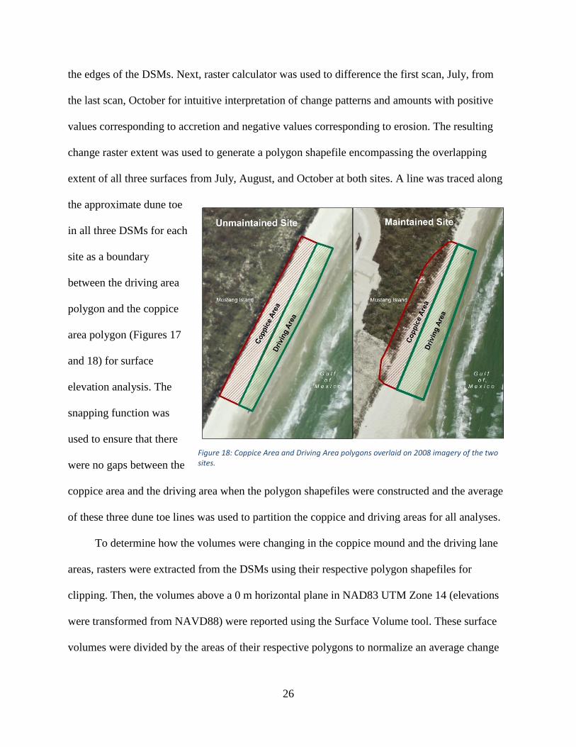
extent of all three surfaces from July, August, and October at both sites. A line was traced along

the approximate dune toe

in all three DSMs for each

site as a boundary

between the driving area

polygon and the coppice

area polygon (Figures 17

and 18) for surface

elevation analysis. The

snapping function was

used to ensure that there

were no gaps between the

coppice area and the driving area when the polygon shapefiles were constructed and the average

of these three dune toe lines was used to partition the coppice and driving areas for all analyses.

To determine how the volumes were changing in the coppice mound and the driving lane

areas, rasters were extracted from the DSMs using their respective polygon shapefiles for

clipping. Then, the volumes above a 0 m horizontal plane in NAD83 UTM Zone 14 (elevations

were transformed from NAVD88) were reported using the Surface Volume tool. These surface

volumes were divided by the areas of their respective polygons to normalize an average change

Figure 18: Coppice Area and Driving Area polygons overlaid on 2008 imagery of the two sites.

27

in elevation for the maintained coppice dune area, the maintained driving lane area, the

unmaintained coppice dune area, and the unmaintained driving lane, the maintained study site,

and the unmaintained study site. July elevations were differenced from October such that

positive changes represented accretion from July to October while negative changes represented

erosion from July to October.

Table 1: Average point spacings were calculated using the Point File Information Tool in ArcGIS for original un-clipped and filtered LAS file. The average number of points per square meter reflects the number of points in the LAS file divided by the area of the shapefile polygon including both the driving area and coppice area.

Date Maintained

Point Spacing

Unmaintained

Point Spacing

Maintained

Points/m2

Unmaintained

Points/m2

July 0.19 m 0.10 m 115 393

August 0.15 m 0.10 m 116 387

October 0.13 m 0.12 m 125 386

CHAPTER III: RESULTS

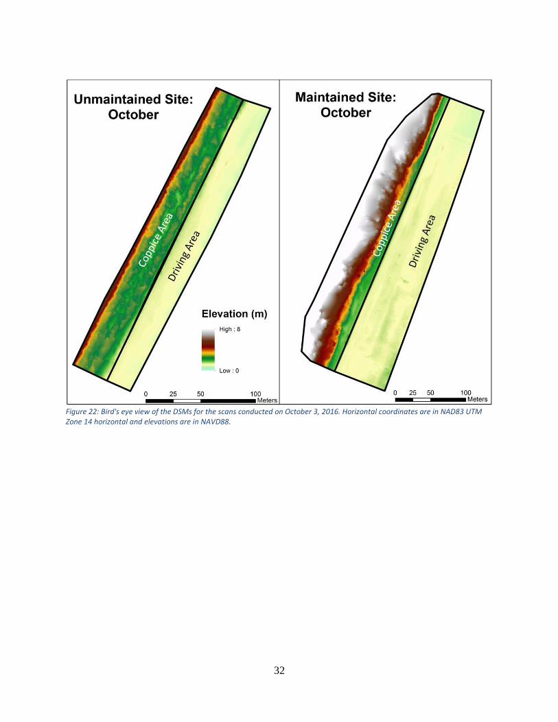
A total of 8 DSMs were generated, one for each site and each month that was surveyed

(Figures 19-22) and a change raster for each site (Figures 23-25). The DSMs for the maintained

site map an area of 52,233.91 m2 while the DSMs for the unmaintained site map an area of

16,659.43 m2. The reason the area for the maintained site is more than three times larger than the

area of the unmaintained site is largely due to the larger driving lane area, which is

approximately 70-m-wide as opposed to the approximately 10-m-wide driving lane at the

unmaintained site (Figure 27). Dune-toe-to-foredune-ridge transect lengths are similar,

approximately 40 m; however, the shapes of the profiles are not. At first glance the three

maintained DSMs for July, August, and October are distinct from the three unmaintained DSMs.

All of the maintained DSMs have a steeper foredune stoss slope (Figure 31 and Table 5), less

vegetation (Figures 27 and 28), and a vast driving lane (Figure 27). All of the unmaintained

DSMs display a gradual stoss foredune slope that gives way to dense vegetation in two

28

somewhat distinct ridges, and a narrow driving lane. The change rasters also exposed differences

in the locations of erosion and deposition across the backbeach from July to October (Figure 25).

At the maintained site (Figure 25), the color of the driving lane as well as the values in Table

2, indicate that it has mostly lost sediment while the unmaintained site the driving lane has

almost equal amounts of erosion and accretion with slightly more accretion meaning that it has

stayed relatively stable with marginal elevation gains. The scale and intensities of the colors

indicate that the greatest elevation changes have largely been in the 30 cm range in most places

with a notable exception being the location of the dune walkover at the maintained site (bottom

left in Figure 25) where accretion was closer to one meter. It is also worth noting that the color

intensities in Figures 23-25 and the values in Table 2 indicate that maintenance causes more

29

Figure 19: Bird’s eye view of DSMs of maintained (top right) from the berm to the foredune ridge and bird’s eye view of unmaintained sites (top left) from the wet dry line to the foredune ridge in NAD83 UTM Zone 14 (horizontal) and NAVD88 (vertical) obtained on July 22, 2016. Oblique images looking alongshore of the July DSM for the unmaintained site (bottom left) and maintained site (bottom right) Note: differences in foredune slope, width of driving lanes, and vegetation.

30

Figure 20: Bird's eye view of the DSMs for the scans conducted on July 22, 2016. Horizontal coordinates are in NAD83 UTM Zone 14 horizontal and elevations are in NAVD88.

31

Figure 21: Bird's eye view of the DSMs for the scans conducted on August 10, 2016. Horizontal coordinates are in NAD83 UTM Zone 14 horizontal and elevations are in NAVD88.

32

Figure 22: Bird's eye view of the DSMs for the scans conducted on October 3, 2016. Horizontal coordinates are in NAD83 UTM Zone 14 horizontal and elevations are in NAVD88.

33

Figure 23: Change DSMs showing the change in elevation from July to August. Areas that are red experienced erosion while areas that are blue experienced accretion.

34

Figure 24: Change DSMs showing the change in elevation from August to October. Areas that are red experienced erosion while areas that are blue experienced accretion.

35

Figure 25: Change DSMs showing the change in elevation from July to October. Areas that are red experienced erosion while areas that are blue experienced accretion.

36

Figure 26: Transect lines generated using the Interpolate Line Tool in ArcGIS. Again, note the differences in slope and driving lane width. Both profiles come from Transect 4 in July at their respective sites (see Figures 30 and 32 for Transect locations).

transport of sediment than natural processes. The maintained driving lane lost an average of -3.3

cm across its entire surface while the unmaintained driving lane gained an average of 0.7 cm

over its entire surface (Table 2). The locations in the driving lane at the unmaintained site that

have lost the most sediment are located on the wet sand beach where cusps from waves have

been carved and along the dune toe where summer traffic is the heaviest. Similarly, the driving

lane of the maintained site has lost increasingly more sand closest to the Zahn Road access road

(Figure 25) while the maintained coppice dune area has gained a substantial 20.0 cm across its

entire surface (Table 2), which is corroborated by the disproportionate amount of blue to red in

the coppice dune polygon.

37

Along the dune toe, there is a blue band that runs the length of the driving lane at the dune

toe and extends approximately 10 m landward but its exact location varies with the location of

the continuous band of accretion near the dune toe. To measure the elevation change of this area,

a shapefile polygon was created to outline this area of accretion on the July to October change

raster (Figure 29). This shapefile was used to extract the surface elevations from the October

DSM and the surface elevations from the July DSM using the Surface Volume tool with a plane

height of zero. The volume of the July surface was subtracted from the volume, which was

normalized using the area of the shapefile polygon to report the elevation change. This area

gained 19.0 cm from July to October, which indicates that a substantial portion of the accretion

at the maintained site took place at the foot of the dune where maintenance was performed

(Figure 29).

Figure 28: Maintained site coppice area looking from the dune towards the Gulf of Mexico. Notice the sparse vegetation in the coppice area in the center of the picture.

Figure 27: Unmaintained site coppice area looking from the dune towards the Gulf of Mexico. Notice the dense vegetation in the coppice area in the center of the picture.

38

Table 2: Changes in surface elevations for maintained coppice area, maintained driving area, maintained study area, unmaintained coppice area, unmaintained driving area, and unmaintained study area.

Change in Surface Elevation (cm)

7/22/16-

8/10/16

8/10/16-

10/3/16

7/22/16-10/3/16

(Total)

Maintained Coppice 10.8 9.1 20.0

Maintained Driving 7.6 -10.9 -3.3

Unmaintained Coppice 2.3 -1.7 0.6

Unmaintained Driving 2.6 -1.9 0.7

Total Maintained 9.2 -1.5 7.7

Total Unmaintained 1.2 -0.9 0.3

Figure 29: The black line outlines the dune mask polygon used to calculate the volume of sand accreted at the base of the dune from July to October.

39

The coppice area of the maintained site had less vegetation as well as fewer species of

plants than the coppice area of the unmaintained site. The maintained site had Croton capitatus,

Heterotheca subaxillaris, Ipomea stolonifera, and Impomea prescaprae while the unmaintained

site had Heterotheca subaxillaris, Ipomea imperati, Impomea prescaprae, Ipomea stolonifera,

Panicum amarum, Croton capitatus, Amaranthus greggi, Sporobulus viginicus, Uniola

paniculata, Sesuviam portulacastrum, Coccoloba uvifera, and Cakile geniculate. The maintained

site had four different species of vegetation, most of which were stoloniferous pioneer species,

on the stoss slope of the foredune while the foredune stoss slope of the unmaintained site had

eleven species, many of which were non-pioneer rhizomatous species (Moreno-Casasola, 1988).

In addition to the differences in sediment transport and vegetation, there were stark contrasts

between the appearances of the profiles for the maintained and unmaintained sites (Figures 26,

27, 28, 31, and 33) that reflect the compound effects of several years of maintenance. As

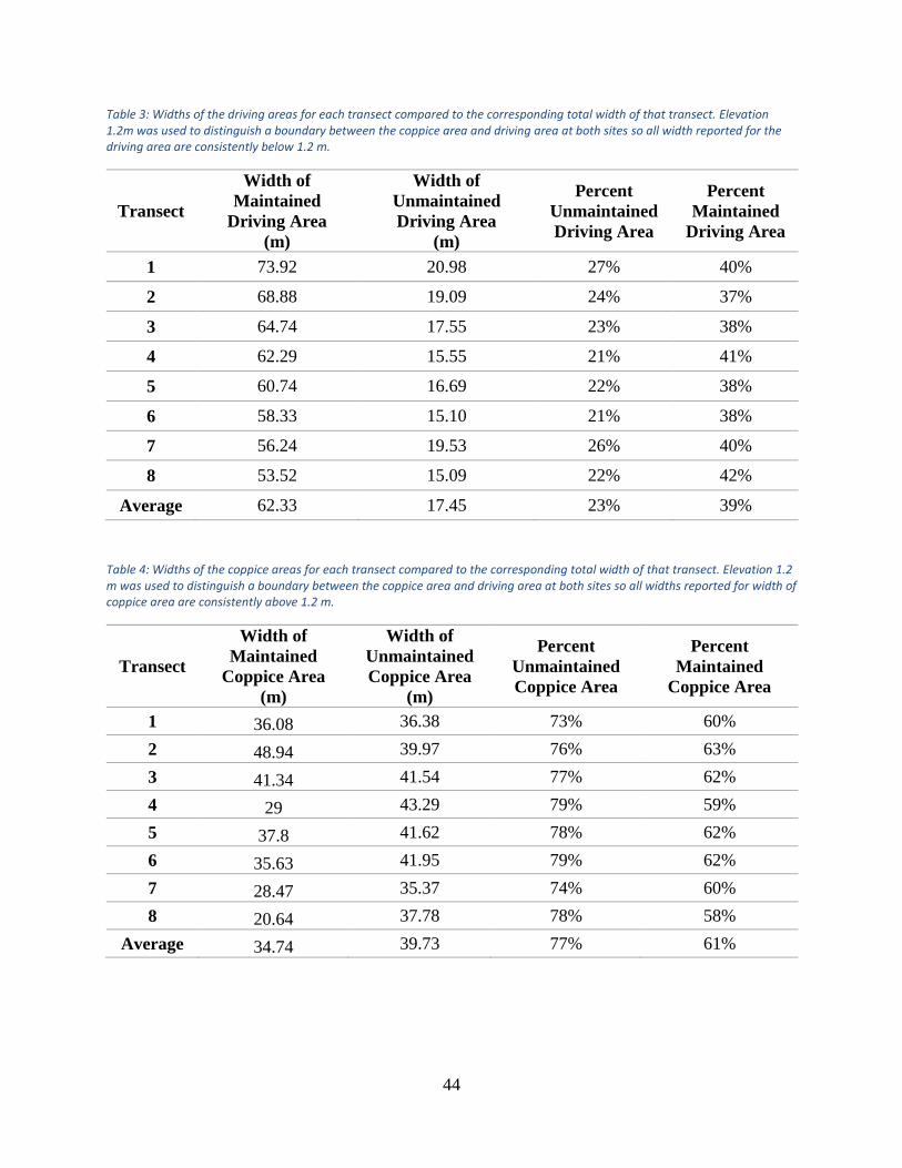
mentioned, the driving lane is wide in the maintained site and narrow in the unmaintained site.

Using an elevation of 1.2 m as the boundary between driving lane and coppice area, it was

determined that the driving area occupies 21-27% of the unmaintained beach study area and 37-

42% of the maintained beach study area (Table 3), but there are also glaring dissimilarities in the

steepness of coppice dune profiles. The slopes (Table 4) of the coppice dune profiles of the

maintained site range from 5.5-14.3 and increase to the north, indicating spatial dependence,

while the slopes of the unmaintained site are all around 6 (Figures 31 and 33). Slopes of the

dune profiles at each site were calculated by dividing the difference in the highest profile

elevation and 1.2 m by the distance in transect length between the highest elevation and the last

landward elevation of 1.2 m. Finally, the unmaintained site is at its most dissipative or gradual

profile in August while the maintained site never accumulates much sand on its sand flat and

40

berm area and its stoss face accretes through October (Figures 34 and 35), which given the water

level data indicating hurricane and storm events, it would be highly unlikely that the coppice area

would accrete naturally during this period. Water levels increase seasonally in the fall (Figure

43) as does storm activity. Hurricane Hermine can be identified in Figure 43 as the higher water

levels at the end of August 2016 and a large storm system can also be identified at the end of

September 2016. These storm events should have resulted in erosion of both the driving lane and

coppice area.

41

Figure 30: DSM of the maintained site for July indicating the locations of the transects drawn using the Interpolate Line Tool. Colors of transect lines correspond to colors on Figure 31.

Figure 31: Graph of Transects 1-8 at the maintained site extracted from the July DSM. Note: Slope increases from Transect 1 to 8.

0

1

2

3

4

5

6

7

0 20 40 60 80 100 120

Elev

atio

n (

m)

Distance from Wet/Dry Line (m)

Maintained Site Transects

Transect 1

Transect 2

Transect 3

Transect 4

Transect 5

Transect 6

Transect 7

Transect 8

42

0

1

2

3

4

5

6

7

0 10 20 30 40 50 60

Elev

atio

n (

m)

Distance from Wet/Dry Line (m)

Unmaintained Site Transects

Transect 1

Transect 2

Transect 3

Transect 4

Transect 5

Transect 6

Transect 7

Transect 8

Figure 33: Graph of Transects 1-8 at the maintained site extracted from the July DSM. Note: No discernable trend exists from Transect 1 to 8.

Figure 32: DSM of the unmaintained site for July indicating the locations of the transects drawn using the Interpolate Line Tool. Colors of the transect lines correspond to color in Figure 33.

43

Figure 34: Transect 8 of the maintained site illustrating that accretion continues to occur in October.

Figure 35: Transect 8 of the unmaintained site indicated that accretion peaks in August.

44

Table 3: Widths of the driving areas for each transect compared to the corresponding total width of that transect. Elevation 1.2m was used to distinguish a boundary between the coppice area and driving area at both sites so all width reported for the driving area are consistently below 1.2 m.

Transect

Width of

Maintained

Driving Area

(m)

Width of

Unmaintained

Driving Area

(m)

Percent

Unmaintained

Driving Area

Percent

Maintained

Driving Area

1 73.92 20.98 27% 40%

2 68.88 19.09 24% 37%

3 64.74 17.55 23% 38%

4 62.29 15.55 21% 41%

5 60.74 16.69 22% 38%

6 58.33 15.10 21% 38%

7 56.24 19.53 26% 40%

8 53.52 15.09 22% 42%

Average 62.33 17.45 23% 39%

Table 4: Widths of the coppice areas for each transect compared to the corresponding total width of that transect. Elevation 1.2 m was used to distinguish a boundary between the coppice area and driving area at both sites so all widths reported for width of coppice area are consistently above 1.2 m.

Transect

Width of

Maintained

Coppice Area

(m)

Width of

Unmaintained

Coppice Area

(m)

Percent

Unmaintained

Coppice Area

Percent

Maintained

Coppice Area

1 36.08 36.38 73% 60%

2 48.94 39.97 76% 63%

3 41.34 41.54 77% 62%

4 29 43.29 79% 59%

5 37.8 41.62 78% 62%

6 35.63 41.95 79% 62%

7 28.47 35.37 74% 60%

8 20.64 37.78 78% 58%

Average 34.74 39.73 77% 61%

45

Table 5: Slopes of the dune profiles at each site calculated by dividing the difference in the highest profile elevation and 1.2 m by the distance in transect length between the highest elevation and the last landward elevation of 1.2 m.

Transect Maintained Foredune Slope Unmaintained Foredune Slope

1 8.8̊ 6.1̊

2 5.8̊ 6.5̊

3 7.2̊ 5.9̊

4 10.2̊ 5.5̊

5 8.1̊ 6.2̊

6 8.4̊ 6.1̊

7 12.6̊ 6.8̊

8 14.3̊ 6.2̊

Average 9.4̊ 6.1̊

Although it was not initially a goal of this study to evaluate long-term effects of maintenance,

it would be remiss not to address the differences in the rates of dune advancement that were

apparent when the DSMs were superimposed on satellite imagery from 2008 (Figure 36). It is

clear when the DSMs are placed on top of basemap imagery that the foredune of the

unmaintained site has advanced farther and more consistently seaward than the maintained site

foredune. When sampled at several locations using the measuring tool in ArcGIS, the distance

seaward from the 2008 vegetation line to the 2016 vegetation line at the maintained site was

approximately 17 m in the center, 28 m at the south end, and 9 m at north end. At the

unmaintained site, dune advance was nearly uniformly 30 m seaward of the 2008 vegetation line.

However, there may be some uncertainty associated with the exact distances since the pixel

resolution for the imagery is 0.5 m and the creators of the imagery, Texas Orthoimagery Program

46

(TOP) and the USDA National Agriculture Imagery Program (NAIP), report a 3-5m or better

absolute ground control. Thus, these distances may vary up to ±5.5 meters.

Measurement Uncertainty

The RTK GNSS, which was used to measure the positions of the targets to georeference the

DSMs and measure 50 ground truth elevations at each site after each pair of scans were

completed (a total of 150 for each site), had a ±1 cm horizontal uncertainty and a ±2 cm vertical

uncertainty inherent in all measurements as was reported by the Trimble R8 User Guide in 2003.

This is associated with carrier phase signal resolution and satellite position errors that cannot be

rectified by systematic atmospheric or geometric pseudorange corrections. Because the Trimble

R8 was equipped with virtual reference station (VRS) capability, theoretically any spatially

dependent errors should have been eliminated by the computation server responsible for

computing the corrections amassed which for this study was the Western Data Systems private

network at Bob Hall Pier (approximately 3 miles or 5 km from the maintained site and 8 miles or

13 km from the unmaintained site). Since all measurements were taken less than a kilometer

from the established VRS, the uncertainty associated with the RTK GPS measurements should

not have changed throughout the study site. Therefore, absolute uncertainties associated with the

RTK GPS measurements should have been no more than 1 cm horizontally and 2 cm vertically,

however, there may be differences between the interpolated DSM elevations and the RTK GNSS

measurements associated with sampling technique used to gather the elevation data for the

targets and for the sample ground points.

The overall average difference in elevation between the RTK GPS ground truth points and

the DSM interpolated elevation values for both sites, using all 300 ground truth points collected

for each site was -5.6 cm with an RMSE of 8.5 cm (Table 6). This value was attained by

47

subtracting the DSM elevation from the RTK elevation. At the maintained site the average

difference in elevation and RMSE associated with its 150 ground truth elevations were slightly

smaller -3.8 cm and 6.2 cm, respectively while the unmaintained site average difference in

elevation and RMSE associated with its 150 ground truth elevations were slightly higher than the

total averages for both sites, -7.5 cm and 10.2 cm, respectively. In Figure 37, this is illustrated by

assigning the same x value to an RTK GPS ground truth elevation and its respective interpolated

DSM elevation. In Figures 37, 39, and 41, it is clear that the elevation of the RTK GPS points

fall slightly below the DSM points for the majority of points and there is a greater difference

between these elevations at higher elevations than there is at lower elevations and these

difference are greater overall at the unmaintained site.

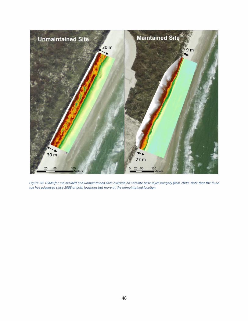
48

Figure 36: DSMs for maintained and unmaintained sites overlaid on satellite base layer imagery from 2008. Note that the dune toe has advanced since 2008 at both locations but more at the unmaintained location.

49

Figure 37: Graph indicating 150 ground truth points from each site paired with their corresponding DSM elevation points and sorted by elevation.

Figure 38: Graph showing the distribution of residuals for both sites.

0

1

2

3

4

5

6

0 50 100 150 200 250 300

Elev

atio

n (

m)

Corresponding Ground Point Number

Methodological Elevation Differences Between RTK and DSM for Both Sites

DSM Elevation

RTK Elevation

-0.35

-0.3

-0.25

-0.2

-0.15

-0.1

-0.05

0

0.05

0.1

0 1 2 3 4 5 6

Res

idu

als

(m)

RTK GPS Elevation (m)

Residual Plot for Both Sites

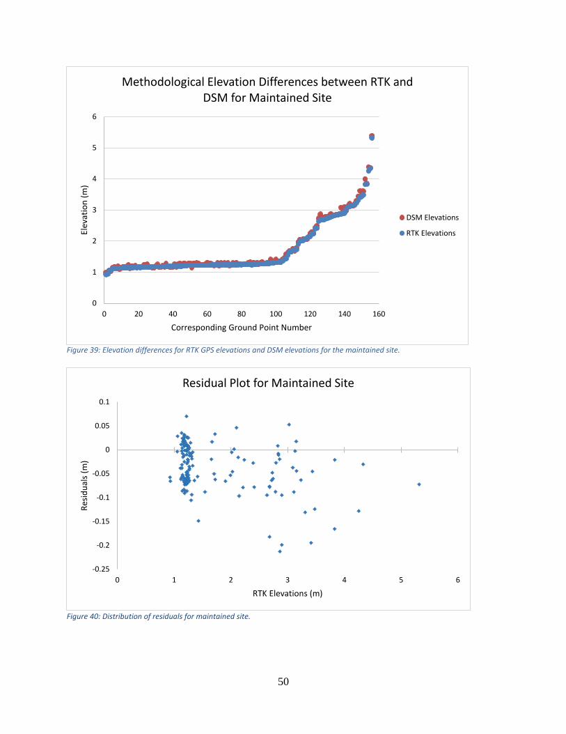
50

Figure 39: Elevation differences for RTK GPS elevations and DSM elevations for the maintained site.

Figure 40: Distribution of residuals for maintained site.

-0.25

-0.2

-0.15

-0.1

-0.05

0

0.05

0.1

0 1 2 3 4 5 6

Res

idu

als

(m)

RTK Elevations (m)

Residual Plot for Maintained Site

0

1

2

3

4

5

6

0 20 40 60 80 100 120 140 160

Elev

atio

n (

m)

Corresponding Ground Point Number

Methodological Elevation Differences between RTK and DSM for Maintained Site

DSM Elevations

RTK Elevations

51

Figure 41: Elevation differences for RTK GPS elevations and DSM elevations for the unmaintained site.

Figure 42: Distribution of residuals for unmaintained site.

0

1

2

3

4

5

6

0 20 40 60 80 100 120 140 160

Elev

atio

n (

m)

Corresponding Ground Point Number)

Methodological Elevation Differences between RTK and DSM for Unmaintained Site

DSM Elevations

RTK Elevations

-0.35

-0.3

-0.25

-0.2

-0.15

-0.1

-0.05

0

0.05

0.1

0 1 2 3 4 5 6

Res

idu

als

(m)

RTK GPS Elevations (m)

Residual Plot for Unmaintained Site

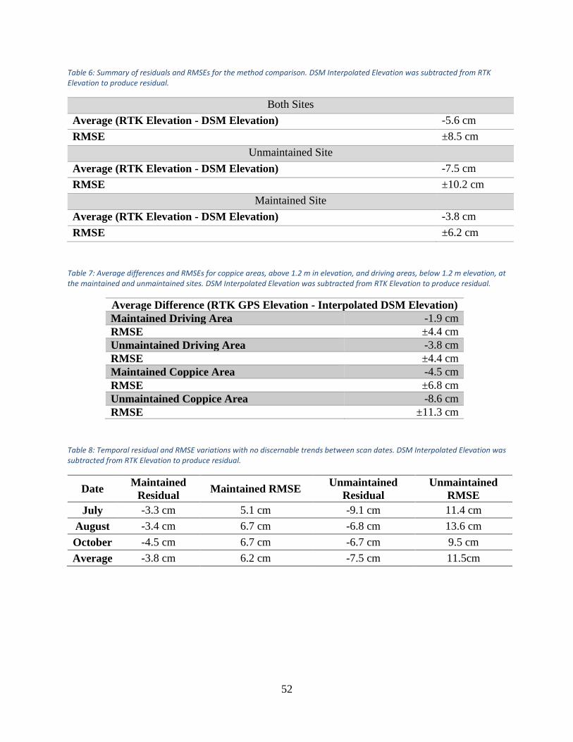
52

Table 6: Summary of residuals and RMSEs for the method comparison. DSM Interpolated Elevation was subtracted from RTK Elevation to produce residual.

Both Sites

Average (RTK Elevation - DSM Elevation) -5.6 cm

RMSE ±8.5 cm

Unmaintained Site

Average (RTK Elevation - DSM Elevation) -7.5 cm

RMSE ±10.2 cm

Maintained Site

Average (RTK Elevation - DSM Elevation) -3.8 cm

RMSE ±6.2 cm

Table 7: Average differences and RMSEs for coppice areas, above 1.2 m in elevation, and driving areas, below 1.2 m elevation, at the maintained and unmaintained sites. DSM Interpolated Elevation was subtracted from RTK Elevation to produce residual.

Average Difference (RTK GPS Elevation - Interpolated DSM Elevation)

Maintained Driving Area -1.9 cm

RMSE ±4.4 cm

Unmaintained Driving Area -3.8 cm

RMSE ±4.4 cm

Maintained Coppice Area -4.5 cm

RMSE ±6.8 cm

Unmaintained Coppice Area -8.6 cm

RMSE ±11.3 cm

Table 8: Temporal residual and RMSE variations with no discernable trends between scan dates. DSM Interpolated Elevation was subtracted from RTK Elevation to produce residual.

Date Maintained

Residual Maintained RMSE

Unmaintained

Residual

Unmaintained

RMSE

July -3.3 cm 5.1 cm -9.1 cm 11.4 cm

August -3.4 cm 6.7 cm -6.8 cm 13.6 cm

October -4.5 cm 6.7 cm -6.7 cm 9.5 cm

Average -3.8 cm 6.2 cm -7.5 cm 11.5cm

53

CHAPTER IV: DISCUSSION

There were several noticeable differences between the transect profiles, DSMs,

volumetric changes, imagery, qualitative observations, rate of seaward dune advancement, and

methodological comparisons of the maintained and unmaintained sites which were the result of

maintenance interrupting seasonal sediment transport patterns and differences in foot and

vehicular traffic. Namely, there were differences in the density and diversity of vegetation in the

coppice area, the stoss slope of the maintained foredune was steeper than the stoss slope of the

unmaintained foredune, the width of the driving lane was much greater at the maintained site

than it was at the unmaintained site, the rate at which the foredune was advancing seaward was

faster at the unmaintained site than it is at the maintained site, and the average difference

between RTK GPS elevations and DSM elevations were smaller for the maintained site than they

were for the unmaintained site.

Vegetation

As mentioned, the maintained site had fewer plant species and sparser vegetation than did

the unmaintained site. The maintained site had four species of plants while the unmaintained site

had eleven species of plants. Most of the species listed, aside from Panicum amarum, Uniola

paniculata, Coccoloba uvifera, and Sporobulus viginicus, are pioneer plant species. The presence

of only pioneer plant species at the maintained site suggests that the foredune is not well-

established. This most likely is the result of excessive foot and vehicular traffic and episodic

burial from maintenance bulldozers but may also result from restrictions on dispersion (Moreno-

Casasola, 1988; Acosta, Carranza, & Izzi, 2009). As shown by the unmaintained site, vegetation

will colonize very close to the wet/dry line if it is not episodically buried, trampled, and crushed

under vehicles. The presence of Panicum amarum, Uniola paniculata, Coccoloba uvifera, and

54

Sporobulus viginicus at the unmaintained site indicate that the foredune is well-established while

the absence of these species indicates that the first dune at the maintained site may not be a

foredune in the traditional sense but a large embryo dune that has been artificially built through

many years of sand amassed through maintenance. In order for a foredune to be well-established

and considered a foredune, it must support woody rhizomatous plant species (Short & Hesp,

1982; Acosta, Carranza, & Izzi, 2009). Woody rhizomatous species require ample shelter,

accumulated organic material from past pioneer species (humus is a good indication that a dune

has existed for some time), and water retention to germinate (Moreno-Casasola, 1988). This

indicates that the maintained site lacks these features as well as species diversity, which also

makes the maintained site less resilient to species-specific destructive forces such as a storm

surge flooding event that exterminates less salt-tolerant species. Because the levels of tourism

and maintenance are the main differences between the maintained and unmaintained sites, the

unmaintained site represents the potential profile of the maintained site if moveable barriers were

constructed at the foot of the dune and maintenance practices were moved seaward (Kelly,

2014). Because the unmaintained site vegetation receives much less traffic and absolutely no

anthropogenic episodic burial events species are allowed to proliferate more readily and trap

more sand for seaward dune advancement since 2008.

Spatial and Temporal Trends

The profiles of both sites exhibited some spatial and temporal dependence. Spatially, at

the maintained site, the slope became increasingly steep from south to north (Figures 30 and 31).

Since this trend as well as stoss steepness is not observed at the unmaintained site, it is likely that

steepening northward and overall steepness at the maintained site is a result of maintenance and

heavier traffic both pedestrian and vehicular. In the southern portion of the maintained site, there

55

is a dune walkover in the location indicated in Figure 25 and people regularly walk up this

portion of the dune resulting in avalanching unconsolidated sand and the more gradual slope

observed at Transects 1, 2, and 3 (Figure 29). Some spatial dependence may also result from the

closer proximity to and longer extent of the Packery Channel jetty about 600 m south of the

study site. It is possible that increased deposition is also greater with proximity to the jetty such

as at Transects 1, 2, and 3 during periods of southern longshore flow and this could partially

explain the greater beach width at the maintained site. An explanation involving natural

processes for this trend’s absence at the unmaintained site is the site is both farther from the jetty

and the jetty does not extend as far into the Gulf of Mexico meaning that the interruption of the

longshore current is diminished and therefore deposition may also be somewhat diminished.

However, the data illustrating the foredune accretion and driving lane erosion (Figure 29)

indicate that maintenance is the primary cause of the characteristic steep slope and lack of

coppice dune area at the maintained site. Dune advancement has also been shown to be inhibited

by maintenance practices. The beach is scraped flat in places that would otherwise form a

coppice area, in this way, maintenance has effectively widened the beach at the maintained site.

Additionally, since the unmaintained site has a gradual slope that is not regularly trampled and

does have a pronounced coppice dune area it can be concluded that the steep stoss slope and lack

of coppice area were almost certainly created by bulldozers that push sand against the dunes

burying vegetation deeply enough and frequently enough that diverse vegetation does not have a

chance to amass. The product is a barren artificial push-up foredune that would otherwise be a

well-developed and densely-vegetated coppice area. The 70 m width of the driving lane at the

maintained site demonstrates that the sediment supply is present and ample for dune

advancement but the lowering of the berm due to maintenance and vehicular traffic has resulted

56

in diminished sediment transport at the berm crest. Due to the lower elevation the berm is

perpetually submerged and the wind’s ability to entrain sand and transport it to the rest of the

beach is greatly reduced. Maintenance and traffic have effectively created a positive feedback

loop to lower the elevation of the driving area of the beach.

Temporally, the unmaintained site (Figure 35 and Table 2) reflected expected seasonal

trends, accreting in July and August and eroding by October when tropical storms occurred and

water levels rose. When each maintained transect was plotted for July, August, and October

(Figure 34 and Table 2), the foredune portion of the beach exhibited an accretional trend through

October, especially near the toe of the dune where is was found the area netted +19 cm (Figure

29). Since maintenance drops off after Labor Day, September 5, 2016, it is possible that this

small increase in elevation in the coppice area from August to October is a result natural

processes where unconsolidated sand becomes suspended over the wide fetch of the driving lane

until it encounters the dune face and is entrapped by the recovering vegetation or is the result of

anthropogenic maintenance that continues into September. Since there is evident erosion of the

driving lane (Figure 24 and Table 2) it is unlikely that the accretion of the coppice area results

from natural aeolian transport and more likely that it is the result of maintenance. Figures 25, 35

and Table 2 illustrate that most of the sedimentary gains were at the dune toe. A more even

distribution would be expected by natural processes. The likely explanation is that as the water

level remains high and bulldozers place sand on the coppice dune area, the lowered beach is

eroded more quickly than is the nourished unmaintained site (Table 2 and Figure 43). If the dune

is attempting to recover, this would suggest that less aggressive maintenance practices and less

traffic would allow the dune vegetation and profile to recover at the maintained site. The width

of the driving lane at the maintained site is approximately 70 m wide while the width of the

57

driving lane at the unmaintained site is approximately 10 m wide. The average two-lane road is

also approximately 10 m wide so if maintenance were progressively performed in a narrower

area closer to the Gulf of Mexico, it is likely that the dunes at the maintained site would advance

and keep pace with the dunes at the unmaintained site. Fences may be highly instrumental in

protecting the dunes and their vegetation as was shown in a study by Kelly in 2014.

Figure 43: Water levels recorded by the Texas Coastal Ocean Observatory Network (TCOON) station at Bob Hall Pier every six minutes during the study period. Water level rises in the fall. Spikes in water level indicate thunderstorms and hurricanes, most notable is Hermine in late August.

Dune Advancement

Since 2008, the foredune at the unmaintained site has advanced considerably farther as a

well as more consistently seaward than the foredune at the maintained site. Because the two sites

are both located north of jetties and near enough to one another to experience similar wind

patterns and wave action the longshore sediment regime should be similarly disrupted at both

sites, which indicates that the cause of this advancement disparity is due to differences in tourism

6.2

6.4

6.6

6.8

7

7.2

7.4

07/19/2016 00:00 08/13/2016 00:00 09/07/2016 00:00 10/02/2016 00:00

Wat

er L

evel

Ab

ove

Bo

b H

all P

ier

Stat

ion

Dat

um

(m

)

Date/Time (mm/dd/yyyy hh:mm)

Water Levels at Bob Hall Pier

58

and maintenance, not an absence of sediment because although the higher dune portion of the

beach has advanced, the shoreline has not changed in any appreciable way since 2008. To

determine this contours at 0.67 meters, the elevation of the wet/dry line (Gibeaut et al., 2001),

were created on the DSM surfaces. At the unmaintained site these contours aligned with 2008

wet/dry line, which was identified visually, and at the maintained site these contours were not

present because the entire study area was above 0.67 m suggesting again that sediment supply

has been ample and stable to the area. It is possible that the wet/dry line may have advanced or

retreated 5.5 m due to the uncertainty associated with the imagery but the point remains that the

dune at unmaintained site has advanced consistently 30 ±5.5 m and the elevation of the flat

portion of the maintained beach has remained above 0.67 m indicating that sediment supply has

been ample at both sites. This is especially true if the spatial dependence of the maintained site is

the result of the additional sand captured by the north side of the Packery Channel jetty,

however, the more parsimonious conclusion from the data is that maintenance and other tourist-

related activities, namely scraping and compacting a wide driving lane and trampling the dunes,

are preventing as much dune advancement from occurring at the maintained site. The transect

data reveal an increase in dune advancement at the maintained site from north to south which is

likely due to maintenance practices since this trend is not present at the unmaintained site. In the

summer, bulldozers often scrape the Zahn Road area from north to south in order to better fill in

the area adjacent to the access road. This results in excess sand from the north being transported

to the south and dispersed against the dune where a dune walkover provides stability to the sand

there. Additionally, winter fronts bring prevailing northern winds, which fuel a southern-flowing

longshore current, and since there is no maintenance to redistribute the sand, it could be that

most of the accretion near Transect 1 of the maintained site occurs in the winter as sand from the

59

longshore current is able to accumulate on the north side of Packery Channel. However, without

scans from the winter this is only speculation.

Method Comparison

The difference between the RTK GPS elevations and the DSM interpolated elevations

can be explained by the sampling method employed when collecting the ground truth elevations.

Target positions were collected at the end of both scans using the RTK GPS. To do this, the R8

was detached from the pole and screwed into the leveled tribrach of a stable tripod such that any

difference in elevation would have been negligible. However, when the ground truth points were

collected, the R8 was attached to the pole and sample points were gathered by walking transects

through the study site and placing the pole in the sand for 10 seconds at a time while the GPS

measured the position of the rover. During this time the topo shoe of the pole sank into the

unconsolidated sand, resulting in elevations that were slightly lower than the passive

measurements of the TLS which is evidenced by mostly negative residuals that resulted from

subtracting DSM interpolated elevations from RTK GPS elevations.

Because the DSM interpolated elevation was subtracted from the RTK GPS elevation, the

negative residuals indicate that overall the DSM surface is slightly higher than the RTK surface

while the few positive residuals most likely indicate areas that were depressed by beach-goers

during the two hours that the scans took place. The bias was not subtracted from interpolated

values since the bias is not consistent between sites or temporally (Table 8) nor was it thought to

improve the DSM elevation. Because the difference resulted from the topo shoe sinking into the

sand the majority of the time, it is possible that DSM elevations are closer to the true elevations

since the laser did not act upon the sand and modify the level of the surface as it measured

elevation.

60

The reason the biases are not consistent between the two sites is because the maintained

site had a greater area of compacted sand as well as less vegetation which differs from the

unmaintained site which had a greater area of unconsolidated sand and more vegetation in a

relatively larger coppice area (Tables 3 and 4) so the overall differences were greater at the

unmaintained site. At both the maintained site and unmaintained site, the topo shoe sank less in

the compacted driving lane and more in the unconsolidated and vegetated coppice area (Table 7).

One could surmise from the smaller differences in both the coppice area and driving area at the

maintained site that maintenance and foot traffic seem to have increased the consolidation of

sand and reduced the vegetation density resulting in a much lower overall differences (Table 6).

The vegetation coupled with the single return setting that was employed by the TLS resulted in

elevations commensurate with vegetation heights where vegetation was present. The DSM was

interpolated using elevations from both vegetation and bare earth since both would be capable of

returning a laser pulse to the TLS but the RTK was placed on the bare earth not floated above the

top of vegetation. Thus, in areas where vegetation was dense, the negative residual resulting

from subtracting the DSM elevation from the RTK elevation would be equal to the height of the

vegetation at that location. Therefore, the residuals at the unmaintained site were much larger

than the residuals at the maintained site because the sand was both less consolidated and the

vegetation was much denser at the unmaintained site.

The average overall difference for both sites (all 300 ground truth points) was

approximately -5.6 cm with an RMSE of 8.5 cm (Table 6), which as stated appears to be a

method-linked sampling bias so the overall uncertainty in the TLS data is most likely close to the

2.8 cm, which accounts for the propagated error of two co-registered scans at the reported

vertical uncertainty of the R8 RTK GPS. Accounting for millimeter range errors and target

61

algorithm differences, the elevations could vary by close to 3 cm meaning that the values

reported in Table 2 could differ from the values reported by up to 3 cm. However, both the data

and uncertainties support a substantial gain in the maintained coppice area so it is likely that the

other values which would result from the logical extrapolation of the processes at work, although

somewhat obscured by the uncertainties, are close to the true values since the changes on the

unmaintained beach reflect the expected seasonal trends in the sediment budget for a dissipative

coast. Additionally, the driving lane of the maintained site was continuously scraped and

compacted so it is believable that its elevation was diminished as the coppice area, which

received the scraped sand, grew.

CHAPTER V: CONCLUSION

The data clearly indicated that morphology of the beackbeach was affected by maintenance

practices. Bulldozing the beach surface resulted in elevation losses in the driving lane area of the

beach where there should have been gains during the summer. It also resulted in substantial gains

in the coppice dune area, when there should have only been small gains, diminished vegetation,

and a steepened stoss foredune slope. The data suggests, although maintenance practices have

been successful with respect to bolstering the dunes and maintaining an impressive height

(Figure 26), if maintenance were to decrease or if a narrower driving lane closer to the Gulf of

Mexico were to be maintained, the dunes would advance seaward at a rate comparable to that of

the unmaintained site dunes and vegetation would likely recover and become more diverse as it

was allowed to proliferate. Although, there were 2 cm vertical uncertainties associated with

georeferencing the point clouds as well as error propagation amounting to 2.8 cm associated with

differencing the DSMs both with 2 cm vertical uncertainties, the results and deliverables are

62

logically plausible. The reported elevation changes are reasonable in that the gains of the

unmaintained site reflect the established seasonal trends and the smaller losses in elevation in the

driving lane at the maintained site, although uncertain, follow logically from the larger more

certain gains over the smaller coppice area. It is even possible that the DSM elevations are more

accurate than the ground truth measurements since the laser does not disturb the surface that is

being measured.

Presently, maintenance practices on Mustang Island have very little influence on the presence

of abundant sediment on its beaches but sediment-deprived communities may find more

meaningful applications for this study other than simple dune protection or municipality cost-

reduction if maintenance were less frequent. Since maintenance has been shown to increase

sediment transport, illustrated by the significantly larger changes in elevation on the maintained

site, and increase the overall volume of unconsolidated sand, the maintenance performed on

Mustang Island may not be appropriate for eroding beaches and some practices may be entirely

counter-productive such as pushing sand into the ocean to be captured and carried away by the

longshore current. Additionally, the sparse vegetation produced by burial coupled with the lower

berm elevation produced by maintenance and traffic at an erosional site like Surfside, Texas

would drastically reduce the available dry sand for transport to the dune and the lack of

vegetation on the dune would be incapable of anchoring the pittance of traveling sand to fortify

and elevate the dune and creating a positive sediment starvation feedback loop.

Despite being short in temporal extent, this study did successfully identify morphological

differences between maintained and unmaintained beaches. In the future, studies of beach

morphology would benefit from a longer monitoring period, a moderately maintained site being

incorporated, scans performed before and after Memorial Day and Labor Day (before and after

63

the prime beach-going season), and the addition of a third scan position at the foredune crest. A

longer monitoring period would prove or disprove theories that accretion at the southern portion

of the maintained site takes place during the winter months when maintenance is not performed

and likely indicate the origin of the sediment. A longer study period would also allow for

tracking seasonal changes in vegetation and morphological changes in the winter, changes

unrelated to maintenance because the beach is not typically groomed from November to April. A

moderately maintained site would indicate how a high maintenance beach would be likely to

respond to less frequent maintenance, which may be valuable information to city planners

looking to reduce expenditures. Because Mustang Island is a popular location for tourism, scans

before and after the most attractive beach holidays would indicate how the beach responds to the

most intense maintenance and highest traffic volumes, which would be useful for anticipating a

sustainable tourism carrying capacity. Finally, a third scan position on the foredune crest,

although abandoned for this study in the interest of time, would increase the overall accuracy and

the range of accurate measurements by capturing areas behind the highest vegetation. Penetration

of vegetation could also be improved by using the full waveform echo digitization capabilities of

the Riegl VZ400 and the higher vantage would be capable of gathering reliable points on the

beach face at the maintained site as well as an overall larger area. The increased range of the

third scan position would also allow the targets to be spread farther apart so that a larger area

could receive geodetic control. However, despite these speculations for improvement, this short

study and small study area was successful in concluding that maintenance practices do affect

backbeach morphology by steepening the stoss slope of the foredune, diminishing vegetation,

widening the flat sand portion of the beach, and limiting dune advancement.

64

REFERENCES

Acosta, A., Carranza, M. L., & Izzi, C. F. (2009). Are there habitats that contribute best to plant

species diversity in coastal dunes? Biodiversity and Conservation, 18(4), 1087–1098.

https://doi.org/10.1007/s10531-008-9454-9

Anderson, J. B., Wallace, D. J., Simms, A. R., Rodriguez, A. B., & Milliken, K. T. (2014).

Variable response of coastal environments of the northwestern Gulf of Mexico to sea-

level rise and climate change: Implications for future change. Marine Geology, 352, 348-

366.

Ashton, A., Murray, A. B., & Arnoult, O. (2001). Formation of coastline features by large-scale

instabilities induced by high-angle waves. Nature, 414(6861), 296-300.

Bascom, W., 1964, Waves and beaches — the dynamics of the ocean surface: New York,

Anchor Books, Doubleday, 267 p.

Behrens, E. W., Watson, R. L., & Mason, C. (1977). Hydraulics and Dynamics of New Corpus

Christi Pass, Texas: A Case History, 1972-73. Texas University Port Aransas Marine

Science Institute.

Brown, L. F., Jr., Brewton, J. L., McGowen, J. H., Evans, T. J., Fisher, W. L., and Groat, C. G.

(1976). Environmental geologic atlas of the Texas Coastal Zone — Corpus Christi area:

The University of Texas at Austin, Bureau of Economic Geology, 123 p.

Bullard, F. M. (1942). Source of beach and river sands on Gulf Coast of Texas: Geological

Society of America Bulletin, v. 53, no. 7, p. 1021-1043.

Conaway, C. A, & Wells, J. T. (2005). “Aeolian Dynamics along Scraped Shorelines, Bogue

Banks, North Carolina.” Journal of Coastal Research 21 (2): 242–54.

65

Curray, J.R. (1960). Sediments and history of Holocene transgression, continental shelf,

northwestern Gulf of Mexico. In: Shepard, F.P., Phleger, F.B., van Andel, T.H. (Eds.),

Recent Sediments, Northwestern Gulf of Mexico, pp. 221–266.

Davis, R. A., & Hayes, M. O. (1984). What is a wave-dominated coast? Marine geology, 60 (1-

4), 313-329.

Dugan, J. E. & Hubbard, D. M. (2010). “Loss of Coastal Strand Habitat in Southern California:

The Role of Beach Grooming.” Estuaries and Coasts 33 (1): 67–77.

Dugan, J. E., Hubbard, D. M., McCrary, M.D. & M.O. Pierson, M.O. (2003). “The Response of

Macrofauna Communities and Shorebirds to Macrophyte Wrack Subsidies on Exposed

Sandy Beaches of Southern California.” \iEstuarine, Coastal and Shelf Science 58: 25–

40.

Engelhard, T., & Withers, K. (1997). “Biological Effects of Mechanical Beach Raking in the

Upper Intertidal Zone on Padre Island National Seashore, Texas.” Center for Coastal

Studies, Texas A&M University-Corpus Christi.

Garnero, G., & Godone, D. (2013). Comparisons between different interpolation

techniques. Proceedings of the international archives of the photogrammetry, remote

sensing and spatial information sciences XL-5 W, 3, 27-28.

Gibeaut, J., Del Angel, D., Lord, A., Lupher, B., Lumb, L., Anderson, M. (2015). Mustang and

North Padre Island Beach Maintenance Impacts and Recommendations for Best

Management Practices. Harte Research Institute for Gulf of Mexico Studies, Texas

A&M-Corpus Christi.

Gibeaut, J. C., Hepner, T., Waldinger, R., Andrews, J., Gutierrez, R., Tremblay, T. A., & Xu, L.

(2001). Changes in gulf shoreline position, Mustang, and North Padre Islands, Texas. A

66

report of the Texas Coastal Coordination Council pursuant to National Oceanic and

Atmospheric Administration. Bureau of Economic Geology, The University of Texas,

Austin Texas, 30.

Greaves, H. E., Vierling, L. A., Eitel, J. U. H., Boelman, N. T., Magney, T. S., Prager, C. M., &

Griffin, K. L. (2016). High-resolution mapping of aboveground shrub biomass in Arctic

tundra using airborne lidar and imagery. Remote Sensing of Environment, 184, 361–373.

https://doi.org/10.1016/j.rse.2016.07.026

Grunewald, R., and Schubert, H. (2007). “The Definition of a New Plant Diversity Index for

Assessing Human Damage on Coastal dunes—Derived from the Shannon Index of

Entropy H′.” Ecological Indicators 7 (1): 1–21.

Hayes, M. O. (1979). Barrier island morphology as a function of tidal and wave regime. In S. P.

Leatherman (Ed.), Barrier Islands from the Gulf of St. Lawrence to the Gulf of Mexico

(pp. 1–27). New York: Academic Press.

Hesp, P. (1988). Morphology, dynamics and internal stratification of some established foredunes

in southeast Australia. Sedimentary Geology, 55(1), 17–41.

Hesp, P. (2002). “Foredunes & Blowouts: Initiation, Geomorphology and Dynamics.”

Geomorphology 48 (1-3): 245–68.

Hesp, P. A. (2012). Surf zone-beach-dune interactions. Retrieved from

http://proceedings.utwente.nl/168/

Houser, C., B. Labude, L. Haider, & B Weymer. (2013). “Impacts of Driving on the Beach: Case

Studies from Assateague Island and Padre Island National Seashores.” Ocean & Coastal

Management 71: 33–45.

67

Hummel, S., Hudak, A. T., Uebler, E. H., Falkowski, M. J., & Megown, K. A. (2011). A

comparison of accuracy and cost of LiDAR versus stand exam data for landscape

management on the Malheur National Forest. Journal of Forestry, 109(5), 267–273.

Inman, D. L., & Nordstrom, C. E. (1971). On the tectonic and morphologic classification of

coasts. The Journal of Geology, 79(1), 1–21.

Kelly, J. (2014). Effects of human activities (raking, scraping, off-road vehicles) and natural

resource protections on the spatial distribution of beach vegetation and related shoreline

features in New Jersey. Journal of Coastal Conservation (Springer Science & Business

Media B.V.), 18(4), 383-398.

Lancaster, N., & A. Baas. (1998). “Influence of Vegetation Cover on Sand Transport by Wind:

Field Studies at Owens Lake, California.” Earth Surface Processes and Landforms 23 (1):

69–82.

Lohse, E. A. (1952). Shallow marine sediments of the Rio Grande delta: University of Texas,

Austin, Ph.D. dissertation, p. 113

Lohse, E. A. (1955). Dynamic geology of the modern coastal region, northwest Gulf of

Mexico, inFinding ancient shorelines: Society of Economic Paleontologists and

Mineralogists Special Publication No. 3, p. 99-105.

Mancini, F., Dubbini, M., Gattelli, M., Stecchi, F., Fabbri, S., & Gabbianelli, G. (2013). Using

unmanned aerial vehicles (UAV) for high-resolution reconstruction of topography: the

structure from motion approach on coastal environments. Remote Sensing, 5(12), 6880-

6898.

McAtee, J. W., & Drawe, D. L. (1981). Human impact on beach and foredune microclimate on

North Padre Island, Texas. Environmental Management, 5(2), 121-134.

68

McGowen, J. H., Garner, L. E., & Wilkinson, B. H. (1977). The Gulf shoreline of Texas:

processes, characteristics, and factors in use: The University of Texas at Austin, Bureau

of Economic Geology Geological Circular 77-3, 27 p.

Montagna, P. A., Gibeaut, J. C., & Tunnell, J. W. (2007). South Texas climate 2100: Coastal

impacts. In W. Norwine & K. John (Eds.), South Texas Climate 2100: Problems and

Prospects, Impacts and Implications. Texas A&M University - Kingsville.

Moreno-Casasola, P. (1988). Patterns of plant species distribution on coastal dunes along the

Gulf of Mexico. Journal of Biogeography, 787-806.

Morton, R. A. (1979). Temporal and spatial variations in shoreline changes and their

implications, examples from the Texas Gulf Coast. Journal of Sedimentary

Research, 49(4).

Morton, R. A., & McGowen, J. H. (1980). Modern depositional environments of the Texas coast.

Austin, Texas: Bureau of Economic Geology, Guidebook, 20, 167 p.

Morton, R. A. (1988). Interactions of Storms, Seawalls, and Beaches of the Texas Coast. Journal

of Coastal Research, (Special Issue No. 4), 113–134.

Niedoroda, A. W., Swift, D. J., Hopkins, T. S., & Ma, C. M. (1984). Shoreface morphodynamics

on wave-dominated coasts. Marine Geology, 60(1), 331-354.

Nordstrom, K. F., Gamper, U., Fontolan, G., Bezzi, A., & Jackson, N. L. (2009). Characteristics

of coastal dune topography and vegetation in environments recently modified using

beach fill and vegetation plantings, Veneto, Italy. Environmental management, 44(6),

1121.

Nordstrom, K. F., Jackson, N. L., & Korotky, K. H. (2011). Aeolian sediment transport across

beach wrack. Journal of Coastal Research, 211-217.

69

Paine, J. G., Mathew, S., & Caudle, T. (2012). Historical shoreline change through 2007, Texas

Gulf Coast: rates, contributing causes, and Holocene context. Gulf Coast Association of

Geological Societies Journal, 1, 13–26.

Saunders, K. E., & Davidson-Arnott, R. G. (1990). Coastal dune response to natural

disturbances. In Canadian Symposium on Coastal Sand Dunes (pp. 321-345).

Short, A. D., & Hesp, P. A. (1982). Wave, beach and dune interactions in southeastern

Australia. Marine geology, 48(3-4), 259-284.

Short, A. D., & Hesp, P. A. (1999). Beach and dune stratification. Handbook of beach and

shoreface morphodynamics, 279-292.

Smith, S. D., Harrison, M. A., & Rowland, J. (2011). “The effects of beach scraping on the

infauna of New Brighton beach, northern NSW.” A report for Byron Shire Council. Coffs

Harbour: National Marine Science Centre, Southern Cross University.

Virtanen, J. P., Hyyppä, H., Kurkela, M., Vaaja, M., Alho, P., & Hyyppä, J. (2014). Rapid

prototyping—A tool for presenting 3-dimensional digital models produced by terrestrial

laser scanning. ISPRS International Journal of Geo-Information, 3(3), 871-890.

Watson, R. L. (1971). Origin of shell beaches, Padre Island, Texas. Journal of Sedimentary

Research, 41(4).

Weise, B. R., & White, W. A. (1980). Padre Island National Seashore: a guide to the geology,

natural environments, and history of a Texas barrier island. Austin, Texas: Bureau of

Economic Geology, University of Texas at Austin, 1980.

White, W. A., Morton, R. A., & Holmes, C. W. (2001). A comparison of factors controlling

sedimentation rates and wetland loss in fluvial-deltaic systems, Texas Gulf coast.

Geomorphology, 44, 47–66.

70

Wright, L. D. & Short, A. D. (1984). Morphodynamic variability of surf zones and beaches: A

synthesis. Marine Geology, 56, 93–118.

Wright, L. D., Short, A. D., & Green, M. O. (1985). Short-term changes in the morphodynamic

states of beaches and surf zones: An empirical predictive model. Marine Geology, 62,

339–364.