Smart Equity Investing:Implementing Risk Optimisation Techniques on Strategic Beta Portfolios January 2018

Boris FaysPhD candidate, HEC Liège

Marie LambertAssociate Professor of Finance, HEC LiègeResearch Associate, EDHEC-Risk Institute

Nicolas PapageorgiouProfessor of Finance, HEC Montreal

2

AbstractWe examine the performance of risk-optimisation techniques on equity style portfolios. To form these portfolios, also called Strategic Beta factors by practitioners and data providers, we group stocks based on size, value and momentum characteristics through either independent or dependent sorting. Overall, performing risk-oriented strategies on style portfolios constructed with a dependent sort deliver greater abnormal returns. On average, we observe these strategies to significantly outperform 42% of the risk-oriented ETFs listed on US exchanges, compared to 31% when the risk-oriented strategies are performed on portfolios formed with an independent sort. We attribute the outperformance yielded by dependent sorting to the fact that it provides a better stratification of the set of stocks’ opportunity and diversification properties.

Classification Codes: 370, 380

EDHEC is one of the top five business schools in France. Its reputation is built on the high quality of its faculty and the privileged relationship with professionals that the school has cultivated since its establishment in 1906. EDHEC Business School has decided to draw on its extensive knowledge of the professional environment and has therefore focused its research on themes that satisfy the needs of professionals.

EDHEC pursues an active research policy in the field of finance. EDHEC-Risk Institute carries out numerous research programmes in the areas of asset allocation and risk management in both the traditional and alternative investment universes.

Copyright © 2018 EDHEC

3

IntroductionFor more than 50 years, passive investors have considered capitalisation-weighted (CW) indices to be a suitable proxy for the tangency portfolios, namely the Maximum Sharpe Ratio (MSR) portfolio. Although CW indices provide a simple, cost-effective and intuitive manner to allocate to stocks, they are also exposed to certain inherent weakness, notably their embedded momentum bias (see, for instance, Hsu and Kalesnik (2014)) and their exposure to greater idiosyncratic risks through their larger allocation to certain stocks.

This evidence has incentivised the investors to seek alternative ways to construct equity portfolios. We observe a dual paradigm shift to so called "smart beta strategies" and "style investing" (also called "strategic beta factors"). On the one hand, smart beta strategies provide an alternative weighting scheme for stocks, i.e. alternative way to diversify risk. Although there is no consensus on whether smart beta strategies should be considered as passive or active management, we can all agree that they follow a systematic and rules-based process. Smart beta ranges from scientific diversification (such as the minimum variance portfolio or risk efficient indexing), risk-based heuristic methods (maximum diversification index, diversity-weighted index or risk parity indexing) to fundamental indexing (e.g., using dividend yield as a proxy for asset market value). Recent debates have emerged between those who believe the term “smart beta” is simply marketing hype (Malkiel (2014), Podkaminer (2015)) and those who believe there is true value to these strategies (Amenc, Goltz and Lodh (2016)). On the other hand, strategic beta investing looks to allocate more efficiently to “style” portfolios to capture systemic sources of market risk premiums. This technique has however existed for decades and firms such as Dimensional Fund Analysis have successfully marketed these strategies since the 1980s. But over the last few years, a number of market developments have led to a variety of new and innovative products being offered to investors by asset managers and banks. New investment vehicles such as ETFs, greater market liquidity, lower transaction costs, and increasingly sophisticated investors have all led to a proliferation of these new investment strategies. Yet, the border between smart and strategic beta is not always clear, leading to many sweeping generalities both for and against alternative portfolio construction techniques.

The recent literature categorises these new investment schemes and analyse the potential performance of Smart Beta strategies (reviewed in Section I). These strategies have been implemented at the individual stock level as the equity building block to construct portfolios that aim to satisfy specific investor objectives or gain exposure to specific systematic risk factors (see for instance, Clarke, Silva and Thorley (2013), Arnott, Hsu, Kalesnik, and Tindall (2013)).

Although most of the research and product has focused on establishing stock level characteristics to form style portfolios and stock level optimisation/weighting schemes, investors can also find benefits in performing strategic beta allocations at the portfolio level (Boudt and Benedict (2013)) or even at the asset class level (Ardia et al. (2016)). In fact, Froot and Teo (2008) observe that institutional investors tend to reallocate their funds across style groupings, which suggests that our objective to perform Smart Beta strategies on investment style portfolios may be in line with this reallocation practice of institutional investors. In fact, recent studies have recognised the use of asset or factor portfolios as the new opportunity set (Idzorek and Kowara (2013), Roncalli and Weisang (2016)). To the best of our knowledge, the value-added of working at the equity portfolio level (rather than asset classes or individual assets) when implementing risk-based optimisations and the importance of the sorting method used to construct those portfolios have not been deeply studied. Our paper addresses this gap. We demonstrate that there is potential for performance improvement when performing strategic optimisations on "smart" characteristic-sorted equity portfolios and we then decompose this outperformance.

4

Our theoretical framework builds on the research of Barberis and Shleifer (2003), who demonstrate the natural tendency of investors to allocate funds according to asset categories, and of Berk (2000), who explains that forming groups of stocks into style indices circumvents the burden of estimating large covariance matrices of returns.

Our research contributions to the literature are twofold. First, we contribute to the literature about Smart Beta by reconstructing a proxy for tangent/well-diversified (US equity) market portfolios by applying risk-based strategies to characteristic-sorted equity portfolios (i.e., an opportunity set sorted by market capitalisation, book-to-market ratio and momentum characteristics). This method ensures style neutrality of the investment solution and simplifies the allocation by reducing the errors in the covariance matrix of returns.

Second, we contribute to the literature regarding style investing (Strategic Beta) and provide guidelines for how these style indices (portfolios) should be constructed to improve the potential of any type of optimisation strategy. To this end, we contrast the empirical results of an independent sort, as in Fama and French (1993), with those of a dependent sort (Lambert and Hübner (2013), Lambert, Fays and Hübner (2016)). The construction method used by Fama and French (1993) sets a standard but many of the methodological choices (e.g., breakpoints or asymetrical sort) that the authors use are not intended to produce portfolios with the highest Sharpe ratio for each level of fundamentals. By using the Fama-French methodology, Lambert et al. (2016) uncover that sorting stocks independently based on correlated variables (e.g., the negative correlation between firms’ market equity and book-to-market equity) might lead to very unequal numbers of securities in portfolios and hence to poor diversification in sorted portfolios. To control for the impact of correlated variables on the classifications assigned to firms’ characteristics as well as ensuring a good balance between portfolios, the authors use a dependent sort. This simple but fundamental methodological change enables proper stratification of the US equity opportunity set. Other researchers have also used dependent sorting to group stocks into portfolios. Among others, Daniel, Grinblatt, Titman and Wermers (1997) perform a triple dependent sort on the size, value and momentum characteristics of a stock to construct benchmarks to test the performance of mutual funds, whereas Novy-Marx (2013) briefly review the positive effect of sorting stocks depending on their value and profitability characteristics, and Wahal and Yavuz (2013) apply a dependent sort as a robustness test to construct portfolios according to stocks’ comovement and their past returns. These last authors also motivate the choice of applying a dependent rather than independent sort to control for correlation between the variables to sort.

Our research focuses on stock level US data, allowing us to construct and test strategies using a variety of protocols and thereby draw robust conclusions as to the benefits of investing in portfolios that do not simply rely on market capitalisation as an input. We demonstrate that a dependent sorting methodology also helps to deliver a significantly higher Sharpe ratio for Strategic Beta strategies. We claim that performing asset allocation on well-diversified portfolios is key to avoid exposure to the idiosyncratic risks as often pointed out by the literature for factor investing. Our stratificiation of the equity market allows us to achieve this goal. We decompose the source of the outperformance of Strategic Beta strategies according to four value drivers: the choices of stock classifications (dependent vs independent), the rebalancing frequency, the number of portfolios that stratify the US equity market, and the risk-oriented optimisations used to form a Strategic Beta strategy.

The rest of the paper is organised as follows. Section I presents a literature review regarding risk-based and heuristic assets allocation techniques. Section II describes the opportunity set, i.e. the data and methodology used to construct the characteristic-based portfolios. Section III reviews

the procedure to estimate the covariance matrix implemented in our risk-based optimisations and the methodology used to account for transaction costs. Section IV reports the results of mean-variance spanning tests to evaluate the efficiency of the risk-based strategies across the differnt sorting methodologies. Section V presents implications of the sorting methodologies in term of portfolio diversification. Section VI concludes.

1 Literature ReviewThe seminal work of Markowitz (1952) on Modern Portfolio Theory (MPT) has pioneered the industry of portfolio management regarding the construction of passive portfolios. Under several assumptions1, the MPT describes how the optimal asset allocation can be reached by minimising the risk-return tradeoff of a portfolio and being tangent to the efficient frontier. Popularised by the introduction of Capital Asset Pricing Model (CAPM) and the principle of market’s prices efficiency (Sharpe (1964), Lintner (1965), Mossin (1966)), the “market” portfolio, which weighs assets relative to their market capitalisation, is considered as the optimal mean-variance portfolio. However, a plethora of papers have recently fueled the debate on the sub-optimality of CW allocations when the assumptions of price efficiency is disregarded (see for instance Arnott, Hsu and Moore (2005, p. 85), Hsu (2006)). The recent literature has thus proposed non-capitilisation-weighted strategies to circumvent the drawbacks of CW allocation schemes.

For instance, Amenc, Goltz, Lodh and Martellini (2014) indicate that traditional CW allocations suffer from poor diversification (mainly invested in large capitalisation stocks) and from exposure to uncontrolled sources of risk. One simple way to ensure good diversification and low idiosyncratic risk is to equal weight all of the N constituents of the portfolio. An Equal-Weighted scheme, referred to as “1/N”, is a heuristic method2 that approximates a mean-variance optimality only when the assets have the same expected return and covariances (Chaves et al. (2012)). This naïve weighting scheme has increased in popularity since DeMiguel et al. (2009) demonstrated that none of the “optimal” allocation schemes the authors put under review (Bayesian methods as well as the CW portfolio) significantly outperform out-of-sample the “1/N” portfolio in terms of the Sharpe ratio, and certainty equivalent value. The only advantage that the CW portfolio has is the zero turnover of its buy-and-hold policy, i.e. the investor does not need to trade any assets, compared to the 1/N policy. Moreover, Plyakha, Uppal and Vilkov (2015) decompose the sources of outperformance between CW and 1/N portfolios and suggest that the equal-weighted strategy produces additional returns from the rebalancing frequencies and the embedded reversal strategy it captures. For the simplicity of the strategy, DeMiguel et al. (2009) claim that the 1/N should be defined as a benchmark to evaluate alternative weighting schemes.

Another debated issue around the mean-variance optimality of the CW portfolio concerns the price as a measure of fair value, if one believes that the stock prices do not fully reflect firm fundamentals, then the CW portfolio is sub-optimal because it over- (under) weights over- (under) priced stocks (Hsu (2006)). To integrate this matter, fundamental indexing has led to the creation of characteristics-based indices that weight stocks according to their economic footprints (such as revenues, book values, and earnings). According to Arnott, Hsu and Moore (2005), this new heuristic scheme provides consistently superior mean-variance performance compared to traditional CW indices. Hsu and Kalesnik (2014) demonstrate that among four allocation strategies (i.e., fundamental weight, minimum variance, CW and 1/N), the traditional CW index is the only allocation scheme that produces a negative measure of “skill”. In theory, skill in portfolio management is related to alpha, and by definition, broad indices should not produce any form of abnormal return. However, CW portfolios exhibit (by construction) a drag in their expected returns because the strategy involves buying stocks when prices are high and

51 -The main assumptions refer to unlimited risk-free borrowing and short selling, homogenous preferences, expectations and horizons, no frictions (taxes, transaction costs) and non-tradable assets (social security claims, housing, human capital). Thus, under real-world conditions, the market portfolio may not be efficient according to Sharpe (1991) and Markowitz (2005).2 - A heuristic method is by definition a method that requires resources with lower complexity to obtain a solution that is sufficient but does not guarantee optimality.

6

selling stocks when prices are low. Overall, Graham (2012) and Perold (2007) conclude that if there is some evidence that CW indices can underperform fundamental indices in some time periods, there is no evidence that because of this return drag, they systematically underperform regardless of the period. In reality, fundamental indexing is another method to implement style investing: it produces a significant bias toward distressed stocks (Jun and Malkiel (2007), Perold (2007)). This method therefore has exactly the same risk of concentration as traditional CW portfolios.

Instead of looking at heuristic methods, academics and practitioners have explored risk-based optimisation techniques which simplify the mean-variance estimation process by disregarding (or subistuting) the expected returns of an asset by its volatility (risk). In other words, the techniques assume that the expected return of an asset increases proportionally to its risks. Clarke, Silva and Thorley (2013), Amenc, Goltz and Martellini (2013), Frazzini and Pedersen (2014) have shown evidence that these techniques exploit a recently discovered market anomaly: the low-beta anomaly. The low beta anomaly contradicts the MPT theory in the sense that stocks with high-volatility (high beta) should earn higher returns than low-volatility (low beta) stocks. However, the low beta anomaly shows the opposite is true on many international markets: low risk stocks outperforms high risk stocks (Baker, Bradley and Taliaferro (2014)). Exploiting this market anomaly may thus deliver higher Sharpe ratios than the traditional CW. There are among the risk-based optimisations three common techniques that disregard (or subistute) the expected return by the volatility of an asset and are shown to exploit the low-beta anomaly.

First, the minimum variance portfolio discards the estimation of the expected return and simply focuses on finding the portfolio with the lowest risk. One of its advantages lies in the simplicity of the parameter estimation. Indeed, the objective function of a minimum variance portfolio only requires the estimation of the assets covariance matrix to attribute weights to the portfolio constituents.

Second, the maximum diversification portfolio substitutes the expected returns from the Sharpe ratio by the volatility (risk) of the assets posing the assumptions that the expected return of an asset increases proportionally to its risk (Choueifaty and Coignard (2008)) - here, the standard deviation is a proxy for expected return. Under this hypothesis, the maximum diversification portfolio is the portfolio that is tangent to the efficient frontier (the MSR portfolio).

Third, the risk parity is the most widely adopted and touted risk-based portfolio allocation. Risk parity aims to equalise the marginal contribution of each asset to the global portfolio risk (Maillard, Roncalli and Teïletche (2010)). Asness, Frazzini and Pedersen (2012) provide a theoretical foundation for risk parity portfolios: in the presence of leverage-averse investors, safer assets should outperform riskier ones on a risk-adjusted basis. Risk parity overweights safer assets to achieve an equal risk contribution between asset classes. For example, if we consider a stock/bond portfolio, risk parity will overweight the allocation to bonds, because it it is the asset class with the lower volatility. Such a strategy would obviously benefit greatly from a decreasing interest rate environment, as has been the case for the last 30 years (Chaves, Hsu, Li and Shakernia (2011), Fisher, Maymin and Maymin (2015)). Nevertheless, traditional risk parity strategies do not come without risk, as risk parity implies not only a low concentration in asset holdings but also a low concentration in risk contributions (Steiner (2012)). It can therefore be a low diversified portfolio in the MPT sense.

Table 1 recalls the analytical forms of the heuristic and risk-based allocations that will serve as a practical base in our empirical analysis, namely minimum variance, risk parity, maximum diversification and equal weighting.

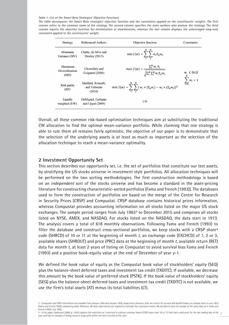
Table 1: List of the Smart Beta Strategies’ Objective FunctionsThe table decomposes the Smart Beta strategies’ objective function and the constraints applied on the constituents’ weights. The first column refers to the common name of the strategy. The second column specifies the main authors who analyse the strategy. The third column reports the objective function for minimisation or maximisation, whereas the last column displays the unleveraged long-only constraint applied to the constituents’ weight.

Overall, all these common risk-based optimisation techniques aim at substituting the traditional CW allocation to find the optimal mean-variance portfolio. While claiming that one strategy is able to rule them all remains fairly optimistic, the objective of our paper is to demonstrate that the selection of the underlying assets is at least as much as important as the selection of the allocation technique to reach a mean-variance optimality.

2 Investment Opportunity SetThis section describes our opportunity set, i.e. the set of portfolios that constitute our test assets, by stratifying the US stocks universe in investment style portfolios. All allocation techniques will be performed on the two sorting methodologies. The first construction methodology is based on an independent sort of the stocks universe and has become a standard in the asset-pricing literature for constructing characteristic-sorted portfolios (Fama and French (1993)). The databases used to form the construction of portfolios are based on the merge of the Centre for Research in Security Prices (CRSP) and Compustat. CRSP database contains historical prices information, whereas Compustat provides accounting information on all stocks listed on the major US stock exchanges. The sample period ranges from July 19633 to December 2015 and comprises all stocks listed on NYSE, AMEX, and NASDAQ. For stocks listed on the NASDAQ, the data start in 1973. The analysis covers a total of 618 monthly observations. Following Fama and French (1993) to filter the database and construct cross-sectional portfolios, we keep stocks with a CRSP share4 code (SHRCD) of 10 or 11 at the beginning of month t, an exchange code (EXCHCD) of 1, 2 or 3, available shares (SHROUT) and price (PRC) data at the beginning of month t, available return (RET) data for month t, at least 2 years of listing on Compustat to avoid survival bias Fama and French (1993) and a positive book-equity value at the end of December of year y-1.

We defined the book value of equity as the Compustat book value of stockholders’ equity (SEQ) plus the balance-sheet deferred taxes and investment tax credit (TXDITC). If available, we decrease this amount by the book value of preferred stock (PSTK). If the book value of stockholders’ equity (SEQ) plus the balance-sheet deferred taxes and investment tax credit (TXDITC) is not available, we use the firm’s total assets (AT) minus its total liabilities (LT).

7

3 - Compustat and CRSP information are available from January 1950 and January 1926, respectively. However, after we correct for survival and backfill biases, our sample starts in July 1953 (Fama and French (1993) rebalancing date). Moreover, 60 daily observations are required to estimate the covariance matrix. We decided to start the sample at the same date as in Fama and French (1993): July 1963.4 - In his paper, Hasbrouck (2009, p. 1455) explains this restriction as “restricted to ordinary common shares (CRSP share code 10 or 11) that had a valid price for the last trading day of the year, and had no changes of listing venue or large splits within the last 3 months of the year”.

8

Book-to-market equity (B/M) is the ratio of the book value of equity for the fiscal year ending in calendar year y-1 divided by market equity. Market equity is defined as the price (PRC) of the stock times the number of shares outstanding (SHROUT) at the end of June y to construct the size characteristic and at the end of December of year y-1 to construct the B/M ratio.

We also include the extension of the Fama and French's three-factor model by Carhart (1997) with a momentum factor (i.e., a t-2 until t-12 cumulative prior return) to add an additional dimension to our investment style portfolios. The momentum reflects the return differential between the highest and lowest prior-return portfolios.

In the original Fama-French approach, portfolios are constructed using a 2x3 independent sorting procedure: two-way sorting (small and big) on market capitalisation and three-way sorting (low, medium, high) on the book-to-market equity ratio. These style classifications are defined according to NYSE5 stocks exchange only and then applied to the whole sample (AMEX, NASDAQ and NYSE). Six portfolios are constructed at the intersection of the 2x3 classifications and rebalanced on a yearly basis at the end of June.

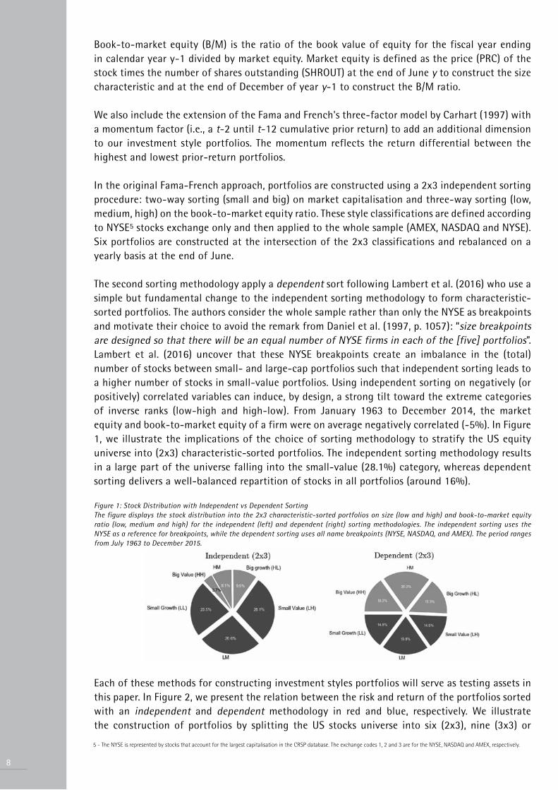
The second sorting methodology apply a dependent sort following Lambert et al. (2016) who use a simple but fundamental change to the independent sorting methodology to form characteristic-sorted portfolios. The authors consider the whole sample rather than only the NYSE as breakpoints and motivate their choice to avoid the remark from Daniel et al. (1997, p. 1057): “size breakpoints are designed so that there will be an equal number of NYSE firms in each of the [five] portfolios”. Lambert et al. (2016) uncover that these NYSE breakpoints create an imbalance in the (total) number of stocks between small- and large-cap portfolios such that independent sorting leads to a higher number of stocks in small-value portfolios. Using independent sorting on negatively (or positively) correlated variables can induce, by design, a strong tilt toward the extreme categories of inverse ranks (low-high and high-low). From January 1963 to December 2014, the market equity and book-to-market equity of a firm were on average negatively correlated (-5%). In Figure 1, we illustrate the implications of the choice of sorting methodology to stratify the US equity universe into (2x3) characteristic-sorted portfolios. The independent sorting methodology results in a large part of the universe falling into the small-value (28.1%) category, whereas dependent sorting delivers a well-balanced repartition of stocks in all portfolios (around 16%).

Figure 1: Stock Distribution with Independent vs Dependent SortingThe figure displays the stock distribution into the 2x3 characteristic-sorted portfolios on size (low and high) and book-to-market equity ratio (low, medium and high) for the independent (left) and dependent (right) sorting methodologies. The independent sorting uses the NYSE as a reference for breakpoints, while the dependent sorting uses all name breakpoints (NYSE, NASDAQ, and AMEX). The period ranges from July 1963 to December 2015.

Each of these methods for constructing investment styles portfolios will serve as testing assets in this paper. In Figure 2, we present the relation between the risk and return of the portfolios sorted with an independent and dependent methodology in red and blue, respectively. We illustrate the construction of portfolios by splitting the US stocks universe into six (2x3), nine (3x3) or

5 - The NYSE is represented by stocks that account for the largest capitalisation in the CRSP database. The exchange codes 1, 2 and 3 are for the NYSE, NASDAQ and AMEX, respectively.

twenty-seven (3x3x3) groups. The 3x3x3 splits is constructed on the size, value and momentum characteristics of a firm. For illustration purposes, portfolios displayed in Figure 2 are rebalanced and reallocated annually.

Figure 2: Characteristic-Sorted Portfolios Risk/Return tradeoffThe figure displays the panels of opportunity sets made of the investment style portfolios based on the sorting methodology. The x-axis reports the annualised standard deviation (in %), and the y-axis reports the annualised average return (in %). Portfolios constructed according to the independent and dependent sorts are displayed in red and blue, respectively. Graphs on the left (right) present the results for cap-weighted (equally weighted) portfolios. We display the opportunity set when the US stock universe is split into six (2x3), nine (3x3) and twenty-seven (3x3x3) groups based on the size and value for the first two splits and the size, value and momentum characteristics of a firm for the triple sort (3x3x3). For the sake of clarity, we only display the portfolio names for the double sorts (2x3 and 3x3). The first letter specifies the size, and the second letter refers to the value characteristic. L, M, and H refer to “Low”, “Medium”, and “High”, respectively.

3 Implementation of Strategic Beta StrategiesOur research focuses on stock level US retrieved from CRSP and Compustat databases, allowing us to construct and test strategies using a variety of protocols and thereby draw robust conclusions as to the benefits of investing in portfolios that do not simply rely on market capitalisation as an input. More precisely, in addition to the choice of the two sorting methodologies to construct portfolios, we control for three other parameters when constructing our style indices.

First, the number of characteristic-based portfolios is set to either six (2x3), nine (3x3), or twenty-seven (3x3x3) and constitute the underlying securities of the final “market” portfolio of our studies. For a large number of securities in a portfolio, the estimation of the covariance matrix requires sophisticated techniques because an estimation solely based on a sample period can be fraught with considerable errors (see, e.g., Ledoit and Wolf (2004)). Referring to the covariance matrix, Berk (2000, p. 420) states that “[g]iven a typical sample of 2000 stocks, this matrix has more than

9

10

2 million elements. With only 70 years of data, there is an obvious specification problem”. He thus suggests grouping stocks to reduce this specification problem. However, this approach does not entirely resolve the issue because the sample covariance matrix has to estimate n(n-1)/2 pair-wise correlations. Increasing the number of groups of stocks can lead to strong sample dependency and consequently noisy estimates. Given that we form 6, 9, and 27 investment style portfolios and use 60 daily returns to estimate the covariance matrix. In the most extreme case (27 portfolios), we are left with 0.17 data points per parameter, which might present a potential issue if we only consider the sample covariance matrix in our optimisations. This problem is also referred to as sampling error. We use, in our applications, the shrinkage methodology from Ledoit and Wolf (2004) to estimate the covariance with lower sampling errors. Further details on the shrinkage method can be found in the Appendix 1.

Second, the allocation scheme intra portfolio is either capitalisation-weighted or equal-weighted. We do this because each allocation scheme has been set as standard throughout the years. For instance, the portfolios found on Ken French’s website are either CW or 1/N.

And third, we control for different rebalancing frequency, i.e. monthly, quarterly, semi-annually, and annually. In their paper on the taxonomy of market equity anomalies, Novy-Marx and Velikov (2016) explain that the recent popularity of equal-weighted portfolios might be misleading after considering transaction costs because a naïve diversification allocation (1/N) places more weights on small-cap stocks, i.e. the most illiquid and expensive stocks to trade. Moreover, a higher rebalancing frequency may cannibalise a large part of the performance of a strategy on net returns (after transactions costs). To consider transaction costs, Plyakha et al. (2015) implement a decreasing function of transaction costs from 1% in 1978 to 0.5% in 1993 for their S&P500 sample. However, in our paper, we trade stocks on NYSE-NASDAQ-AMEX exchanges and consequently have to differentiate transactions costs for small and large-cap stocks. We thus follow an approach similar to that of Novy-Marx and Velikov (2016) and use the individual stocks estimates from the Gibbs sampling developed in Hasbrouck (2009). Further details on this method can be found in the Appendix 2.

In Figure 3, we show the annual box-and-whisker plot for the CRSP/Gibbs estimates of transaction costs (variable c from equation (5)) from 1963 to 2015.

Figure 3: Variation of Transaction Cost Estimates Following Hasbrouck (2009)The figure presents a box plot of the distribution of individual stocks transaction costs estimated as in Hasbrouck (2009). The sample period ranges from 1963 to 2015. The whiskers represent the distribution of the 5th to 95th percentile, and the upper and lower edges of the boxes correspond to the 25th and 75th percentiles. The gray dots represent outliers.

Novy-Marx and Velikov (2016) uncover a minor drawback to Hasbrouck’s estimation technique, which requires relatively long series of daily prices to perform the estimation (250 days). This results in a number of missing observations for which Novy-Marx and Velikov (2016) perform a non-parametric matching method and attribute equivalent transaction costs to the stock with a missing value according to its closest match in size and idiosyncratic volatility. Since these missing observations represents only 4% of the total market capitalisation universe, instead, we decided to simply replace the missing values with transaction costs of 0.50%. We employ this (extreme) arbitrary value because (1) we see from Figure 3 that none of the estimates ever breach a trading cost of 50 bps since 1963, (2) this choice will more strongly impact illiquid stocks with short amount of daily observations (small-capitalisation stocks) and (3) Plyakha, Uppal and Vilkov (2015) also choose to set this threshold for transaction costs from 1993 onwards.

In Table 2, we report the transaction costs for our Strategic Beta strategies. We distinguish the implication of transaction for rebalancing the investment style portfolios on a monthly (1), quarterly (3), semi-annually (6) or annual (12) basis. We also examine the trading costs according to the number of constructed portfolios, namely, six (2x3), nine (3x3), and twenty-seven (3x3x3). The results are presented in annual terms (in %) and show that transaction costs have a linear relationship with the rebalancing frequency according to the Patton and Timmermann (2010) test for decreasing monotonic relationships. The level of transaction costs is also greater for portfolios sorted dependently and suggests that small stocks have higher weights with dependent sorting.

Table 2: Strategic Beta and Transaction CostsThe table reports the annual transaction costs (in %) for the four different Strategic Beta strategies: equal-weighted (EW), maximum diversification (MD), minimum variance (MV), and risk parity (RP). These strategies are applied on portfolios sorted independently or dependently. These portfolios can be rebalanced on a monthly (1), quarterly (3), semi-annually (6) or annual (12) basis. Finally, the number of portfolios is either six (2x3), nine (3x3) or twenty-seven (3x3x3). We also report the Patton and Timmermann (2010) test for decreasing monotonic relationships.6 The sample period ranges from July 1963 to December 2015.

11

6 - Matlab code is made available on Prof. Patton’s website.

12

To summarise, each sorting methodology (independent and dependent) generates 24 combinations of portfolios whom will constitute our test assets for performing the heuristic and risk-based optimisations. From these 24 combinations of constructing investment styles portfolios, we apply the four different allocation techniques defined in Table 1 of Section I, namely, minimum variance, maximum diversification, risk parity, and equally weighted. In total, the combinations of strategies are equal to 96 for each methodology of portfolio construction.

After adjusting our US sample for well-known biases, delisting return, survivorship bias, etc., and controlling for a variety of protocols to construct Strategic Beta strategies, we expect a dependent sorting methodology to outperform a independent sorting because the allocation of a dependent sort is not contingent on the correlations between the sorted variables. Such that, the dependent sort shows a strong stability in the stock allocation among the style portfolios. The diversification properties of the style portfolios constructed from the dependent sorting methodology are thus expected to be greater in comparison to an independent sort.

4 Mean-Variance Spanning TestTo test the outperformance of one sorting methodology versus the other, we build on a traditional mean-variance spanning test introduced by Huberman and Kandel (1987) which differentiates whether adding one security to a set of investment improves the efficient frontier. Although it is important for an investor to know whether her set of opportunity increases with a new asset, it might be interesting to know whether the source of improvement comes either from the tangent or global minimum-variance (GMV) portfolio. Indeed, the two-fund separation theorem (Tobin (1958)) tells us that if an investor has access to a risk-free asset, he should only interested in the portfolio with the highest Sharpe ratio. According to his risk-preferences, his optimal allocation should lie on the Capital Market Line (CML) and be composed of a mix of the tangent portfolio (MSR) and the risk-free asset. However, if all capital is invested in risky assets, the optimal portfolio lies on the efficient frontier and is dependent on the investor utility and degree of risk aversion.

Kan and Zhou (2012) establish a mean-variance spanning test based on a step-down approach that allows us to differentiate whether the source of improvement in the efficient frontier comes from the tangent and/or the GMV portfolio. This is only when both portfolios are improved that we observe a shift of the entire opportunity set.

The elegance of the step-down spanning tests lies in its ability to determine whether adding N elements to a set of K assets improves the tangent and/or GMV portfolio. The regression spanning test can be written as (1)

where is the benchmark portfolios composed of K assets (US Bond and a Portfolio A) and is the set of test assets composed of K+N elements (Portfolio B) . In this paper, K is equal to 2 and N is equal to 1. Kan and Zhou (2012) present the test in matrix notations as follows:

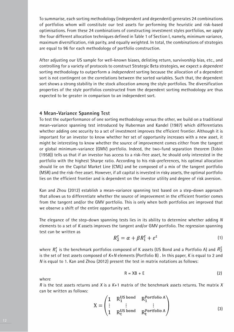
R = XB + E (2)whereR is the test assets returns and X is a K+1 matrix of the benchmark assets returns. The matrix X can be written as follows:

(3)

Finally, B in equation (7) is a , and E is the error term vector (ε1,…, ε1)'.

The first test of the step-down procedure poses the null hypothesis for the tangent portfolio such that α=0N using OLS regression. The tangent portfolio is improved when the null is rejected. (4)

The second test of the step-down procedure poses the null hypothesis for the GMV portfolio. This second test is conditional on the first test, α=0N, and verifies whether δ=1N−β1K=0N. It is only when both conditions are rejected that the test suggests an improvement of the GMV portfolio by adding N assets to the K benchmark assets.

(5)

The term “ ” means conditional.Kan and Zhou (2012) identify a test for statistical significance of the hypothesis similar to a GRS F-test. The F-test for the first hypothesis ( ) is

(6)

where T is the number of observations, K is the number of benchmark assets, N is the number of test assets, , with denoting the variance of the benchmark assets, and takes the same notation as but refers to the benchmark assets plus the new test asset.

The F-test for the second hypothesis ( ) is

(7)

where are the efficient set (hyperbola) constants with for the benchmark assets. In equation (7), , , and are the equivalent

notations for the benchmark assets plus the new test asset.

Figure 4: Improving the Tangency (Panel A) and GMV (Panel B) PortfoliosThe figure displays the spanning illustration for opportunity sets made of a benchmark asset, i.e., the 30-Year US Treasury Bond and Portfolio A, and a test asset, i.e. the benchmark assets plus Portfolio B. The x-axis reports the annualised standard deviation (in %), and the y-axis reports the annualised average return (in %). This example is fictitious but illustrates in Panel A (Panel B) an improvement of the tangency (GMV) portfolio after adding Portfolio B to the benchmark assets.

13

14

We illustrate in Panel A of Figure 4 a significant improvement for the tangency portfolio when a test asset (Portfolio B) is added to the benchmark assets (US bonds and Portfolio A). Panel B indicates a significant improvement for the GMV portfolio when a test asset (Portfolio B) is added to the benchmark assets (US bonds and Portfolio A). The original graphical illustrations of Kan and Zhou (2012, p. 158) explain in more detail how the constants , , and are used to determine the geometric locations of the GMV portfolio.

Intuitively, a spanning of the test assets (K+N) means that the weight attributed to the N test assets in the portfolio is trivial. Put differently, discarding the N test assets does not significantly change the efficient frontier of the K benchmark assets.

A. Testing Characteristic-Sorted PortfoliosIn Table 3, we summarise the results of the step-down analysis7 applied to the strategies developed in this paper. More precisely, Panel A reports the results when the benchmark assets are 30-Year US Treasury Bonds and a risk-optimisation technique applied to independent portfolios (Portfolio A), whereas the test asset is the same risk-optimisation technique applied to dependent portfolios (Portfolio B). We perform the same analysis in Panel B but in the reverse order, that is, the benchmark assets are now 30-Year US Treasury Bonds and a risk-based strategy constructed on dependent portfolios (Portfolio A), whereas the test asset is now the same risk-based strategy but constructed on independent portfolios (Portfolio B).

It is important to note that each of optimisations can have 12 different combinations of construction according to the choices of rebalancing frequency and number of portfolios. The portfolios can be rebalanced on a monthly (1), quarterly (3), semi-annually (6) or annual (12) basis, and the number of portfolios is either six (2x3), nine (3x3) or twenty-seven (3x3x3). All results are presented net of transaction costs.

The results shown in Panel A (Table 3) demonstrate that applying risk-optimisation techniques to dependent portfolios can significantly improve the tangency portfolio of the benchmark assets for two risk-oriented strategies, that is, maximum diversification (MD) and minimum variance (MV). Indeed, the first hypothesis ( ) is rejected five (nine) out of 12 times for MD on cap-weighted (equal-weighted) portfolios, whereas the rejection for MV optimisation is six (five) out of 12 with cap-weighted (equal-weighted) portfolios.

In Panel B, the results demonstrate that all risk-optimisation techniques applied to independent portfolios never improve the tangency portfolio of the benchmark assets with a confidence level of 95% relative to the same risk-optimisation techniques applied on dependent portfolios.7 - The full analysis is reported in Appendices 3 to 6.

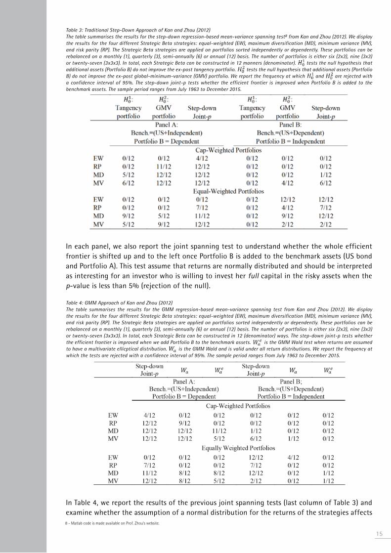
Table 3: Traditional Step-Down Approach of Kan and Zhou (2012)The table summarises the results for the step-down regression-based mean-variance spanning test8 from Kan and Zhou (2012). We display the results for the four different Strategic Beta strategies: equal-weighted (EW), maximum diversification (MD), minimum variance (MV), and risk parity (RP). The Strategic Beta strategies are applied on portfolios sorted independently or dependently. These portfolios can be rebalanced on a monthly (1), quarterly (3), semi-annually (6) or annual (12) basis. The number of portfolios is either six (2x3), nine (3x3) or twenty-seven (3x3x3). In total, each Strategic Beta can be constructed in 12 manners (denominator). tests the null hypothesis that additional assets (Portfolio B) do not improve the ex-post tangency portfolio. tests the null hypothesis that additional assets (Portfolio B) do not improve the ex-post global-minimum-variance (GMV) portfolio. We report the frequency at which and are rejected with a confidence interval of 95%. The step-down joint-p tests whether the efficient frontier is improved when Portfolio B is added to the benchmark assets. The sample period ranges from July 1963 to December 2015.

In each panel, we also report the joint spanning test to understand whether the whole efficient frontier is shifted up and to the left once Portfolio B is added to the benchmark assets (US bond and Portfolio A). This test assume that returns are normally distributed and should be interpreted as interesting for an investor who is willing to invest her full capital in the risky assets when the p-value is less than 5% (rejection of the null).

Table 4: GMM Approach of Kan and Zhou (2012)The table summarises the results for the GMM regression-based mean-variance spanning test from Kan and Zhou (2012). We display the results for the four different Strategic Beta strategies: equal-weighted (EW), maximum diversification (MD), minimum variance (MV), and risk parity (RP). The Strategic Beta strategies are applied on portfolios sorted independently or dependently. These portfolios can be rebalanced on a monthly (1), quarterly (3), semi-annually (6) or annual (12) basis. The number of portfolios is either six (2x3), nine (3x3) or twenty-seven (3x3x3). In total, each Strategic Beta can be constructed in 12 (denominator) ways. The step-down joint-p tests whether the efficient frontier is improved when we add Portfolio B to the benchmark assets. is the GMM Wald test when returns are assumed to have a multivariate ellicptical distribution. is the GMM Wald and is valid under all return distributions. We report the frequency at which the tests are rejected with a confidence interval of 95%. The sample period ranges from July 1963 to December 2015.

In Table 4, we report the results of the previous joint spanning tests (last column of Table 3) and examine whether the assumption of a normal distribution for the returns of the strategies affects

15

8 - Matlab code is made available on Prof. Zhou’s website.

16

our results. Kan and Zhou (2012) describe two extensions when returns are not assumed to be normally distributed and exhibit excess kurtosis. Using the moment conditions, they apply a GMM method to estimate the regression parameters of equation (7). The first test is a joint F-test based on the results from the last column of Table 3. Recall that in this case, the returns are assumed to obey a normal distribution and the test is a joint test on the whole efficient frontier. In the first column of both panels (A and B), the level of rejection is high owing to an improvement in the global minimum variance. The second column is a GMM Wald test for returns under general distributions9 ( ). The last column is a GMM Wald test in which returns are assumed to follow an elliptical distribution ( ) and that controls for heteroscedasticity and excess kurtosis. Moving from the first column to the last, we see that rejection rates of spanning only decrease in Panel B, not in Panel A, indicating that there are over-rejection problems in the first column of Panel B (Table 4) because the returns are assumed to obey a normal distribution. Yet, the rejection rates in Panel A appears to remain stable across the assumptions about the return distribution of the strategies.

B. Testing Against the US ETF UniverseWe retrieve data about the US ETF universe from Morningstar and classify it according to the Morningstar® Strategic Beta classification tool. Table 5 reports the Strategic Beta definitions from Morningstar Guide10. The last column of the table specifies the category used in this paper to categorise the ETF universe. There are four categories: (1) Risk-weighted, (2) Return-oriented, (3) Blended, and (4) Other. We also report in parentheses the number of ETFs that fall in each category.

Table 5: Morningstar® Strategic Beta ClassificationThe table identifies the Strategic Beta classifications provided by the data provider Morningstar®. The first column report whether the categorisation of Strategic Beta is applicable to an ETF. The second column identifies the specific attribute of the ETF strategy, and the last column specifies the broader category used in this paper to categorise the ETF universe. There are four categories: (1) risk-weighted, (2) return-oriented, (3) other, and (4) blended. We also mention in parentheses the number of ETFs that fall under the broader category groups.

Concerning the treatment of the database, we winsorise the 1st and 99th percentile of return at each available month date and then remove returns lower than -100 percent and higher than 100 percent to lower the impact of outliers and reporting issues. Finally, we keep ETFs with more than one year of observations. Our tests are based on monthly returns, and all returns are denominated in US dollars.

9 - For more details, see Kan and Zhou (2012, p. 171) and Chen, Chung Ho, Hsu (2010). See also Chen, Ho, and Wu (2004) for GMM step-down resolution.10 - The Morningstar Strategic Beta guide can be find on this website.

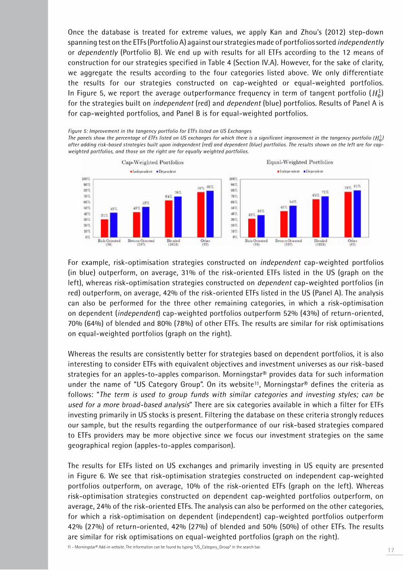
Once the database is treated for extreme values, we apply Kan and Zhou’s (2012) step-down spanning test on the ETFs (Portfolio A) against our strategies made of portfolios sorted independently or dependently (Portfolio B). We end up with results for all ETFs according to the 12 means of construction for our strategies specified in Table 4 (Section IV.A). However, for the sake of clarity, we aggregate the results according to the four categories listed above. We only differentiate the results for our strategies constructed on cap-weighted or equal-weighted portfolios. In Figure 5, we report the average outperformance frequency in term of tangent portfolio ( ) for the strategies built on independent (red) and dependent (blue) portfolios. Results of Panel A is for cap-weighted portfolios, and Panel B is for equal-weighted portfolios.

Figure 5: Improvement in the tangency portfolio for ETFs listed on US ExchangesThe panels show the percentage of ETFs listed on US exchanges for which there is a significant improvement in the tangency portfolio ( ) after adding risk-based strategies built upon independent (red) and dependent (blue) portfolios. The results shown on the left are for cap-weighted portfolios, and those on the right are for equally weighted portfolios.

For example, risk-optimisation strategies constructed on independent cap-weighted portfolios (in blue) outperform, on average, 31% of the risk-oriented ETFs listed in the US (graph on the left), whereas risk-optimisation strategies constructed on dependent cap-weighted portfolios (in red) outperform, on average, 42% of the risk-oriented ETFs listed in the US (Panel A). The analysis can also be performed for the three other remaining categories, in which a risk-optimisation on dependent (independent) cap-weighted portfolios outperform 52% (43%) of return-oriented, 70% (64%) of blended and 80% (78%) of other ETFs. The results are similar for risk optimisations on equal-weighted portfolios (graph on the right).

Whereas the results are consistently better for strategies based on dependent portfolios, it is also interesting to consider ETFs with equivalent objectives and investment universes as our risk-based strategies for an apples-to-apples comparison. Morningstar® provides data for such information under the name of “US Category Group”. On its website11, Morningstar® defines the criteria as follows: “The term is used to group funds with similar categories and investing styles; can be used for a more broad-based analysis” There are six categories available in which a filter for ETFs investing primarily in US stocks is present. Filtering the database on these criteria strongly reduces our sample, but the results regarding the outperformance of our risk-based strategies compared to ETFs providers may be more objective since we focus our investment strategies on the same geographical region (apples-to-apples comparison).

The results for ETFs listed on US exchanges and primarily investing in US equity are presented in Figure 6. We see that risk-optimisation strategies constructed on independent cap-weighted portfolios outperform, on average, 10% of the risk-oriented ETFs (graph on the left). Whereas risk-optimisation strategies constructed on dependent cap-weighted portfolios outperform, on average, 24% of the risk-oriented ETFs. The analysis can also be performed on the other categories, for which a risk-optimisation on dependent (independent) cap-weighted portfolios outperform 42% (27%) of return-oriented, 42% (27%) of blended and 50% (50%) of other ETFs. The results are similar for risk optimisations on equal-weighted portfolios (graph on the right).

1711 - Morningstar® Add-in website. The information can be found by typing “US_Category_Group” in the search bar.

18

Figure 6: Improvement in the tangency portfolio for ETFs listed on US Exchanges and a Category Group named U.S. EquityThe panels show the percentage of ETFs listed on US exchanges and primarily investing in US equities only for which there is significant improvement of the tangency portfolio ( ) after adding risk-based strategies built upon independent (red) and dependent (blue) portfolios. The results shown on the left are for cap-weighted portfolios, and those on the right are for equally weighted portfolios.

In conclusion, a dependent sort to construct investment style portfolios exhibits better risk-return attributes for risk-optimisation strategies. Whereas the majority of ETFs providers logically exhibit equivalent or better selectivity skills than our fully passive strategies on all US stock universes. The next sections disentangle the distinctive characteristics of the two sorting methodologies.

5 Disentangling the outperformance: the diversification properties of the opportunity setsOur spanning tests deliver conclusive results towards better risk-return attributes for dependent portfolios. This section investigates further the diversification properties yielded by the two competing sorting methods. Section A analyses the pair-wise correlations between the portfolios depending on the sorting methodology. Section B estimates the correlation of stocks among the portfolios. Section C reviews the general case of equal-weighted portfolio variance and the implications according to the sorting methodology. Section D quantifies the differences in return yielded by the diversification properties of each sorting procedure.

A. Pair-Wise Correlation of Style PortfoliosIn Figure 7, we illustrate the stock repartition when the number of portfolios is increased either by a larger split of the sample (from a 2x3 to a 3x3) or by adding a new characteristic (3x3x3). Throughout this paper, we followed Lambert et al. (2016) to stratify the US equity universe according to the dimensions of size, value and momentum characteristics. Considering the repartitions of the stocks based on the two sorting methods, we see that using an independent sort results in an imbalanced of stocks across the portfolios, and this effect becomes larger when more groups are constructed.

Figure 7: Stock Distribution with Independent vs Dependent SortingThese plots show the stock distribution among the 3x3 characteristic-sorted portfolios on size (low, medium and high) the book-to-market equity ratio (low, medium and high) for the independent and dependent sorting methodologies. We also report the average percentage of stock repartition among the 3x3x3 characteristic-sorted portfolios when momentum is added as a third variable. For clarity, we group the 27 portfolios according to their size classifications (small, medium, and big). The period ranges from July 1963 to December 2015.

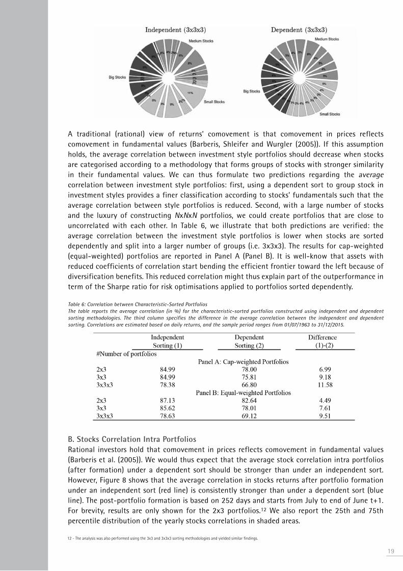
A traditional (rational) view of returns’ comovement is that comovement in prices reflects comovement in fundamental values (Barberis, Shleifer and Wurgler (2005)). If this assumption holds, the average correlation between investment style portfolios should decrease when stocks are categorised according to a methodology that forms groups of stocks with stronger similarity in their fundamental values. We can thus formulate two predictions regarding the average correlation between investment style portfolios: first, using a dependent sort to group stock in investment styles provides a finer classification according to stocks’ fundamentals such that the average correlation between style portfolios is reduced. Second, with a large number of stocks and the luxury of constructing NxNxN portfolios, we could create portfolios that are close to uncorrelated with each other. In Table 6, we illustrate that both predictions are verified: the average correlation between the investment style portfolios is lower when stocks are sorted dependently and split into a larger number of groups (i.e. 3x3x3). The results for cap-weighted (equal-weighted) portfolios are reported in Panel A (Panel B). It is well-know that assets with reduced coefficients of correlation start bending the efficient frontier toward the left because of diversification benefits. This reduced correlation might thus explain part of the outperformance in term of the Sharpe ratio for risk optimisations applied to portfolios sorted dependently.

Table 6: Correlation between Characteristic-Sorted PortfoliosThe table reports the average correlation (in %) for the characteristic-sorted portfolios constructed using independent and dependent sorting methodologies. The third column specifies the difference in the average correlation between the independent and dependent sorting. Correlations are estimated based on daily returns, and the sample period ranges from 01/07/1963 to 31/12/2015.

B. Stocks Correlation Intra PortfoliosRational investors hold that comovement in prices reflects comovement in fundamental values (Barberis et al. (2005)). We would thus expect that the average stock correlation intra portfolios (after formation) under a dependent sort should be stronger than under an independent sort. However, Figure 8 shows that the average correlation in stocks returns after portfolio formation under an independent sort (red line) is consistently stronger than under a dependent sort (blue line). The post-portfolio formation is based on 252 days and starts from July to end of June t+1. For brevity, results are only shown for the 2x3 portfolios.12 We also report the 25th and 75th percentile distribution of the yearly stocks correlations in shaded areas.

19

12 - The analysis was also performed using the 3x3 and 3x3x3 sorting methodologies and yielded similar findings.

20

Figure 8: Yearly Average Stock Returns Correlation after Portfolio FormationThe figure shows that the average correlation in stocks returns after portfolio formation under an independent sort (red line) and a dependent sort (blue line). The post-portfolio-formation period is comprised of 252 days and starts from July to end of June t+1. We also represent by the shaded areas the 25-75th percentile distribution of the yearly stock correlations. The results are displayed for the 2x3 portfolios from 1963 to 2015.

We uncover from this puzzling systematic correlation bias that stock correlation is stronger among securities for which the exchange has the largest total market capitalisation, i.e., the NYSE, NASDAQ and then AMEX, in this order. We plot in Figures 9 and 10 the reparation of stocks belonging to the NYSE, NASDAQ and AMEX in green, red and blue, respectively. Results for the 2x3 portfolios sorted independently and dependently are shown in Figures 9 and 10, respectively.

Figure 9: Stock Distribution in Portfolios Sorted Independently According to the Listed ExchangeThe figure reports the repartitions of stocks belonging to the NYSE, NASDAQ and AMEX in green, red and blue, respectively. The results for the 2x3 portfolios sorted independently are shown.

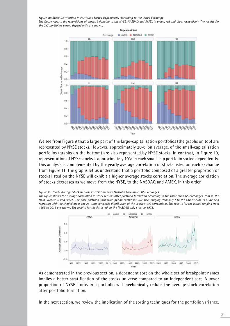
Figure 10: Stock Distribution in Portfolios Sorted Dependently According to the Listed ExchangeThe figure reports the repartitions of stocks belonging to the NYSE, NASDAQ and AMEX in green, red and blue, respectively. The results for the 2x3 portfolios sorted dependently are shown.

We see from Figure 9 that a large part of the large-capitalisation portfolios (the graphs on top) are represented by NYSE stocks. However, approximately 20%, on average, of the small-capitalisation portfolios (graphs on the bottom) are also represented by NYSE stocks. In contrast, in Figure 10, representation of NYSE stocks is approximately 10% in each small-cap portfolio sorted dependently. This analysis is complemented by the yearly average correlation of stocks listed on each exchange from Figure 11. The graphs let us understand that a portfolio composed of a greater proportion of stocks listed on the NYSE will exhibit a higher average stocks correlation. The average correlation of stocks decreases as we move from the NYSE, to the NASDAQ and AMEX, in this order.

Figure 11: Yearly Average Stock Returns Correlation after Portfolio Formation: US ExchangesThe figure shows the average correlation in stock returns after portfolio formation according to the three main US exchanges, that is, the NYSE, NASDAQ, and AMEX. The post-portfolio-formation period comprises 252 days ranging from July t to the end of June t+1. We also represent with the shaded areas the 25-75th percentile distribution of the yearly stock correlations. The results for the period ranging from 1963 to 2015 are shown. The results for stocks listed on the NASDAQ only start in 1973.

As demonstrated in the previous section, a dependent sort on the whole set of breakpoint names implies a better stratification of the stocks universe compared to an independent sort. A lower proportion of NYSE stocks in a portfolio will mechanically reduce the average stock correlation after portfolio formation.

In the next section, we review the implication of the sorting techniques for the portfolio variance.

21

22

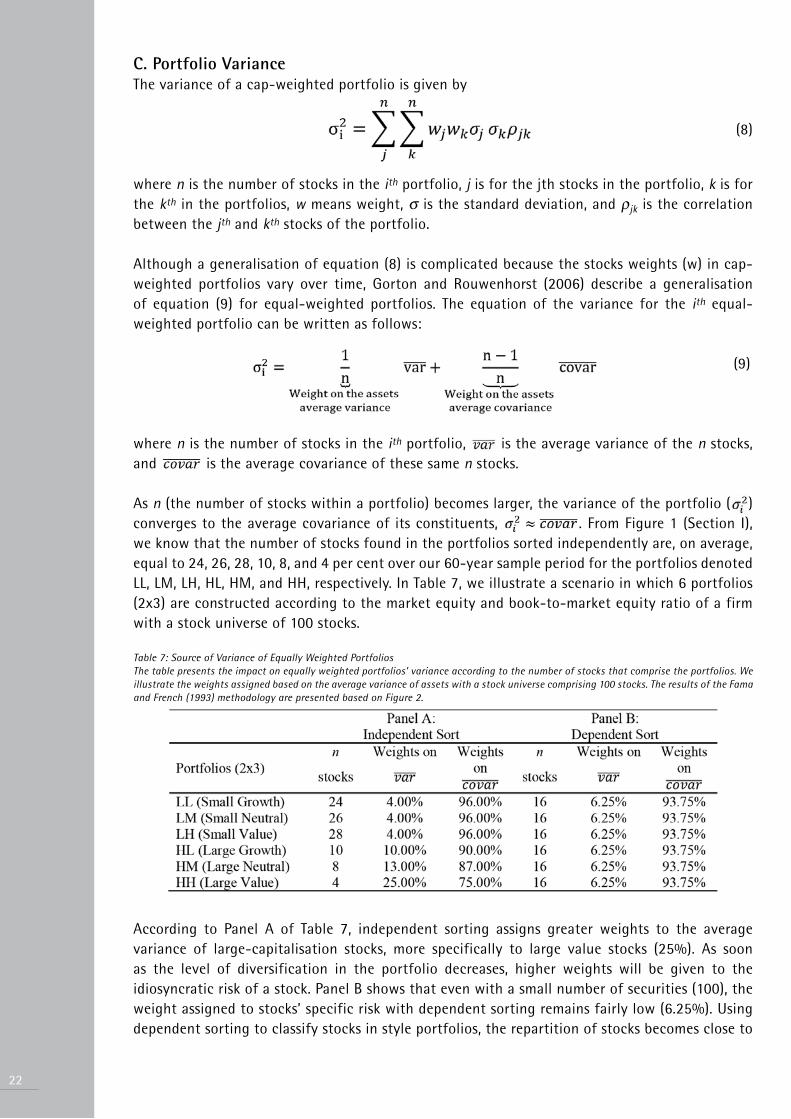
C. Portfolio VarianceThe variance of a cap-weighted portfolio is given by

(8)

where n is the number of stocks in the ith portfolio, j is for the jth stocks in the portfolio, k is for the kth in the portfolios, w means weight, σ is the standard deviation, and ρjk is the correlation between the jth and kth stocks of the portfolio.

Although a generalisation of equation (8) is complicated because the stocks weights (w) in cap-weighted portfolios vary over time, Gorton and Rouwenhorst (2006) describe a generalisation of equation (9) for equal-weighted portfolios. The equation of the variance for the ith equal-weighted portfolio can be written as follows: (9)

where n is the number of stocks in the ith portfolio, is the average variance of the n stocks, and is the average covariance of these same n stocks.

As n (the number of stocks within a portfolio) becomes larger, the variance of the portfolio ( )converges to the average covariance of its constituents, . From Figure 1 (Section I), we know that the number of stocks found in the portfolios sorted independently are, on average, equal to 24, 26, 28, 10, 8, and 4 per cent over our 60-year sample period for the portfolios denoted LL, LM, LH, HL, HM, and HH, respectively. In Table 7, we illustrate a scenario in which 6 portfolios (2x3) are constructed according to the market equity and book-to-market equity ratio of a firm with a stock universe of 100 stocks.

Table 7: Source of Variance of Equally Weighted PortfoliosThe table presents the impact on equally weighted portfolios’ variance according to the number of stocks that comprise the portfolios. We illustrate the weights assigned based on the average variance of assets with a stock universe comprising 100 stocks. The results of the Fama and French (1993) methodology are presented based on Figure 2.

According to Panel A of Table 7, independent sorting assigns greater weights to the average variance of large-capitalisation stocks, more specifically to large value stocks (25%). As soon as the level of diversification in the portfolio decreases, higher weights will be given to the idiosyncratic risk of a stock. Panel B shows that even with a small number of securities (100), the weight assigned to stocks’ specific risk with dependent sorting remains fairly low (6.25%). Using dependent sorting to classify stocks in style portfolios, the repartition of stocks becomes close to

1/n (n is equal to 6) when the breakpoints are the 33rd and 66th percentiles of the distribution for all breakpoint names (NYSE, NASDAQ, and AMEX). Even though this concern may be immaterial for the construction of six portfolios with a universe of more than 3,000 stocks (US), the issue might become important for (1) a greater number of portfolios, (2) the early stage of the sample, or (3) less developed markets.

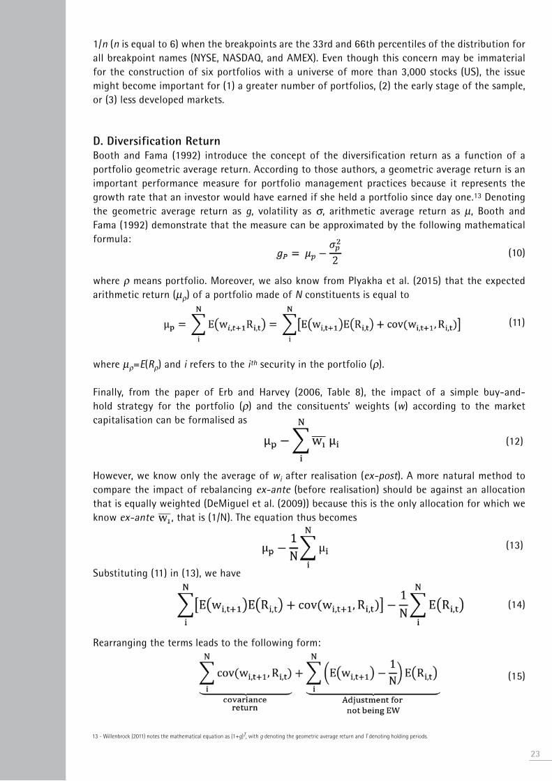
D. Diversification ReturnBooth and Fama (1992) introduce the concept of the diversification return as a function of a portfolio geometric average return. According to those authors, a geometric average return is an important performance measure for portfolio management practices because it represents the growth rate that an investor would have earned if she held a portfolio since day one.13 Denoting the geometric average return as g, volatility as σ, arithmetic average return as µ, Booth and Fama (1992) demonstrate that the measure can be approximated by the following mathematical formula: (10)

where ρ means portfolio. Moreover, we also know from Plyakha et al. (2015) that the expected arithmetic return (µρ) of a portfolio made of N constituents is equal to

(11)

where µρ=E(Rρ) and i refers to the ith security in the portfolio (ρ).

Finally, from the paper of Erb and Harvey (2006, Table 8), the impact of a simple buy-and-hold strategy for the portfolio (ρ) and the consituents’ weights (w) according to the market capitalisation can be formalised as

(12)

However, we know only the average of wi after realisation (ex-post). A more natural method to compare the impact of rebalancing ex-ante (before realisation) should be against an allocation that is equally weighted (DeMiguel et al. (2009)) because this is the only allocation for which we know ex-ante , that is (1/N). The equation thus becomes

(13)

Substituting (11) in (13), we have

(14)

Rearranging the terms leads to the following form:

(15)

23

13 - Willenbrock (2011) notes the mathematical equation as (1+g)T, with g denoting the geometric average return and T denoting holding periods.

24

It is important to note that both terms vanish if we implement an equally weighted strategy that rebalances at each period t (in this study, on a monthly basis).

Finally, Willenbrock (2011) formalises the diversification return as follows:

(16)

where i stands for the ith security in the portfolio (ρ) and g refers to the geometric return.

The concept of diversification in returns emphasises that the geometric average return of a portfolio is greater than the sum of the geometric average return of its constituents. Substituting (10) in (16), we have (17)

Alternatively, we can factorise the equation such that, (18)

Rearranging the terms,

(19)

We can substitute the terms from equations (15) in (19) and rewrite the diversification return as follows:

(20)

Equation (20) provides a benchmark14 to compare a strategy using dynamic weights with the average constituents that it holds. The benefits of applying risk-optimisation strategies (MV, MD, and risk parity) to the passive portfolios can be compared to a naïve diversification allocation (equally weighted). We can isolate whether the incremental return benefit is earned by the weights of the strategy (first and second terms) or the last term, also coined volatility harvesting by Bouchey et al. (2012). The full decomposition of the results can be found in Appendices 7 to 10.

To compare the benefits of diversification between the two sorting methodologies, we adjust the diversification return according to the risk of the benchmark sorting methodology. In this paper, we use the independent sorted portfolios as a benchmark. Equation (21) describe the risk-adjustment for comparing the diversification return.

(21)

14 - This test is implemented on gross returns. The decomposition in equation (20) does not hold when transaction costs are considered.

In short, if the spread (πDR) is positive, a dependent sort to construct portfolios delivers greater diversification benefits on a risk-adjusted basis than an independent sort. In Table 8, we report the results for four Strategic Beta strategies and the combination of rebalancing frequency, number of portfolios and portfolios allocation (cap-weighted and equal-weighted). The spreads are strictly positive in 92 of 96 strategies. Risk-oriented strategies specifically designed to maximise the objective of diversification (max. div.) yields (logically) the best results.

Table 8: Spread in Risk-adjusted Diversification ReturnsThe table reports the spread of diversification return from equation (21) for the four different Strategic Beta strategies: equal-weighted (EW), maximum diversification (MD), minimum variance (MV), and risk parity (RP). These strategies are applied on portfolios sorted independently or dependently. These portfolios can be rebalanced on a monthly (1), quarterly (3), semi-annually (6) or annual (12) basis. Finally, the number of portfolios is either six (2x3), nine (3x3) or twenty-seven (3x3x3). The sample period ranges from July 1963 to December 2015.

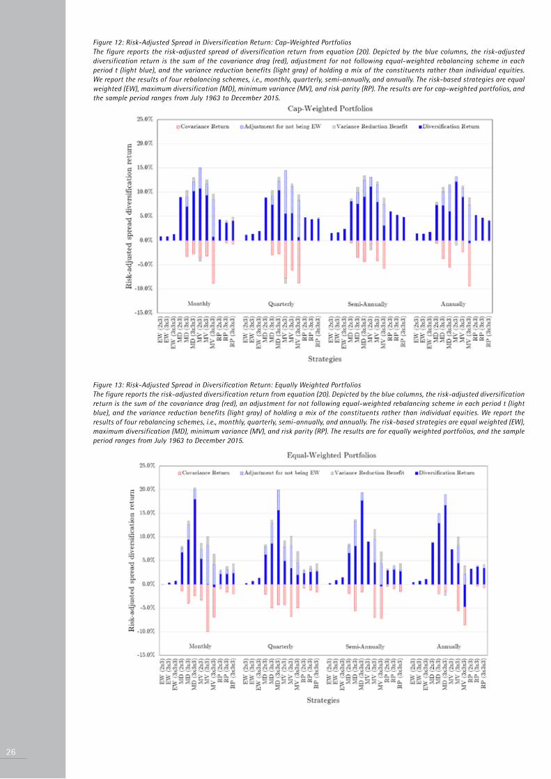
Figures 12 and 13 let us visualise the global results for all the risk-based strategies on cap-weighted and equal-weighted portfolios, respectively. On a risk-adjusted basis, we see that the covariance drag (light red columns) is smaller for portfolios sorted dependently. However, for most of the strategies, the adjustment for not being equally weighted (light blue columns) and the variance reduction benefit (light gray columns) are typically greater for dependently sorted portfolios.

25

26

Figure 12: Risk-Adjusted Spread in Diversification Return: Cap-Weighted PortfoliosThe figure reports the risk-adjusted spread of diversification return from equation (20). Depicted by the blue columns, the risk-adjusted diversification return is the sum of the covariance drag (red), adjustment for not following equal-weighted rebalancing scheme in each period t (light blue), and the variance reduction benefits (light gray) of holding a mix of the constituents rather than individual equities. We report the results of four rebalancing schemes, i.e., monthly, quarterly, semi-annually, and annually. The risk-based strategies are equal weighted (EW), maximum diversification (MD), minimum variance (MV), and risk parity (RP). The results are for cap-weighted portfolios, and the sample period ranges from July 1963 to December 2015.

Figure 13: Risk-Adjusted Spread in Diversification Return: Equally Weighted PortfoliosThe figure reports the risk-adjusted diversification return from equation (20). Depicted by the blue columns, the risk-adjusted diversification return is the sum of the covariance drag (red), an adjustment for not following equal-weighted rebalancing scheme in each period t (light blue), and the variance reduction benefits (light gray) of holding a mix of the constituents rather than individual equities. We report the results of four rebalancing schemes, i.e., monthly, quarterly, semi-annually, and annually. The risk-based strategies are equal weighted (EW), maximum diversification (MD), minimum variance (MV), and risk parity (RP). The results are for equally weighted portfolios, and the sample period ranges from July 1963 to December 2015.

6 ConclusionsMotivated by the need to reduce the number of assets in portfolio optimisations, we implement smart beta strategies on “style” portfolios as the equity building block. This approach not only reduces the issues in estimating a large covariance matrix of returns but also is consistent with the common practice of institutional investors, who tend to reallocate funds across style groupings (see, for instance, Froot and Teo (2008)). We show that the methodology for grouping stocks in different style buckets has strong implications for the performance of the final strategy. To categorise stocks in investment style portfolios, we stratify the universe along the dimensions of size, value and momentum characteristics. We implement two sorting methodologies to construct characteristic-based portfolios: traditional independent sorting according to Fama and French (1993) and dependent sorting according to Lambert et al. (2016). To demonstrate the implications of the sorting methodologies, we apply mean-variance spanning tests from Kan and Zhou (2012) on the risk-oriented strategies that use characteristic-based portfolios as assets (or Strategic Beta strategies). The results show that dependent sorting of stocks in portfolios provides significantly higher Sharpe ratios for risk-oriented Strategic Beta strategies. The results hold regardless of whether stocks are capitalisation-weighted or equal-weighted in portfolios, whether stocks are rebalanced at different frequencies or whether returns are net of transaction costs. Because dependent sorting controls for correlated variables and stratifies the stock universe in well-diversified portfolios (Lambert et al. (2016)), this sorting methodology delivers better diversification benefits for Strategic Beta strategies. To demonstrate this point, we provide a decomposition of the diversification return from Booth and Fama (1992). We uncover that the diversification return is, on a risk-adjusted basis, higher for Strategic Beta strategies implemented on dependent portfolios than on independent portfolios.

Appendices

Appendix 1Estimation of the Covariance MatrixWe briefly describe in this section a shrinkage methodology used in our applications to estimate the covariance with lower sampling errors following Ledoit and Wolf (2004). In their model, the authors build on Elton and Gruber (1973) who use a constant correlation coefficient to shrink the assets’ covariance toward a global average correlation estimator

The constant correlation coefficient is determined using,

(22)

where N is the number of portfolios - in our applications, either 6, 9 or 27. The term is the historical correlation estimate between the ith portfolio and the jth portfolio.

Ledoit and Wolf (2004) then obtain an optimal structure for the covariance matrix and reduce the sampling error of a traditional sample covariance matrix (S):

(23)

where Σ is the output covariance matrix from the shrinkage estimation and δ is the optimal shrinkage intensity.15 S is the sample covariance matrix from our 60 daily returns, and F is the structured covariance matrix with assets’ covariance estimated via the constant correlation

27

15 - Matlab code is made available at Prof. Wolf’s website.

28

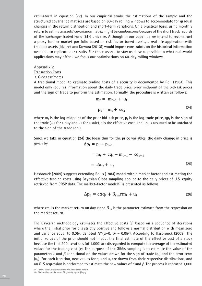
estimator16 in equation (22). In our empirical study, the estimations of the sample and the structured covariance matrices are based on 60-day rolling windows to accommodate for gradualchanges in the return distribution and short-term variations. On a practical basis, using monthly return to estimate assets’ covariance matrix might be cumbersome because of the short track records of the Exchange-Traded Fund (ETF) universe. Although in our paper, as we intend to reconstruct a proxy for the market portfolio based on risk-factor-based assets, a real-life application with tradable assets (Idzorek and Kowara (2013)) would impose constraints on the historical information available to replicate our results. For this reason - to stay as close as possible to what real-world applications may offer - we focus our optimisations on 60-day rolling windows.

Appendix 2Transaction Costs1. Gibbs estimatesA traditional model to estimate trading costs of a security is documented by Roll (1984). This model only requires information about the daily trade price, prior midpoint of the bid-ask prices and the sign of trade to perform the estimation. Formally, the procedure is written as follows:

(24)

where mt is the log midpoint of the prior bid-ask price, pt is the log trade price, qpt is the sign of the trade (+1 for a buy and -1 for a sale), c is the effective cost, and upt is assumed to be unrelated to the sign of the trade (qpt).

Since we take in equation (24) the logarithm for the price variables, the daily change in price is given by

(25)

Hasbrouck (2009) suggests extending Roll’s (1984) model with a market factor and estimating the effective trading costs using Bayesian Gibbs sampling applied to the daily prices of U.S. equity retrieved from CRSP data. The market-factor model17 is presented as follows:

(26)

where rmt is the market return on day t and βrm is the parameter estimate from the regression on the market return.

The Bayesian methodology estimates the effective costs (c) based on a sequence of iterations where the initial prior for c is strictly positive and follows a normal distribution with mean zero and variance equal to 0.052, denoted N+(µ=0, σ2 = 0.052). According to Hasbrouck (2009), the initial values of the prior should not impact the final estimate of the effective cost of a stock because the first 200 iterations (of 1,000) are disregarded to compute the average of the estimated values for the trading cost (c). The purpose of the Gibbs sampling is to estimate the value of the parameters c and β conditional on the values drawn for the sign of trade (qt) and the error term (ut). For each iteration, new values for qt and ut are drawn from their respective distributions, and an OLS regression is performed to estimate the new values of c and β .The process is repeated 1,000 17 - The SAS code is made available on Prof. Hasbrouck’s website.16 - The covariance of the matrix F is given by .

times, and the final value for c is the average of the last 800 estimations of the procedure. For more information on the iterative process, we refer to Hasbrouck (2009, p. 1447), who summarises the procedure in four steps.18

Appendix 3The table reports the results for the step-down regression-based mean-variance spanning test from Kan and Zhou (2012). We display the results when the benchmark assets are 30-Year US Treasury Bonds and the Strategic Beta on independent cap-weighted portfolios. The test assets have the same Strategic Beta on dependent cap-weighted portfolios. In total, there are four different Strategic Beta strategies: equal-weighted (EW), maximum diversification (MD), minimum variance (MV), and risk-parity (RP). These portfolios can be rebalanced on a monthly (1), quarterly (3), semi-annually (6) or annual (12) basis. The number of portfolios is either six (2x3), nine (3x3) or twenty-seven (3x3x3). The first column reports the correlation between Strategic Beta on both sorting methodologies. F1 tests the null hypothesis that additional tests asset do not improve the ex-post tangency portfolio. F2 tests the null hypothesis that additional test assets do not improve the ex-post global-minimum-variance (GMV) portfolio. We also report the step-down joint-p, which tests whether the efficient frontier is improved when we add the test asset to the benchmark assets. is the GMM Wald test when returns are assumed to have a multivariate ellicptical distribution; the results are comparable to those for the step-down joint-p. is the GMM Wald and is valid under all return distributions. The sample period ranges from July 1963 to December 2015.

29

18 - Further details regarding the application of the estimation technique can also be found in Marshall, Nguyen and Visaltanachoti (2011) and Novy-Marx and Velikov (2016).

30

Appendix 4The table reports the results for the step-down regression-based mean-variance spanning test from Kan and Zhou (2012). We display the results when the benchmark assets are 30-Year US Treasury Bonds and the Strategic Beta on independent equally weighted portfolios. The test assets have the same Strategic Beta on dependent equally weighted portfolios. In total, there are four different Strategic Beta strategies: equal-weighted (EW), maximum diversification (MD), minimum variance (MV), and risk-parity (RP). These portfolios can be rebalanced on a monthly (1), quarterly (3), semi-annually (6) or annual (12) basis. The number of portfolios is either six (2x3), nine (3x3) or twenty-seven (3x3x3). The first column reports the correlation between Strategic Beta on both sorting methodologies. F1 tests the null hypothesis that additional test assets do not improve the ex-post tangency portfolio. F2 tests the null hypothesis that additional test assets do not improve the ex-post global-minimum-variance (GMV) portfolio. We also report the step-down joint-p, which tests whether the efficient frontier is improved when we add the test asset to the benchmark assets. is the GMM Wald test when returns are assumed to have a multivariate elliptical distribution; the results are comparable to those for the step-down joint-p. is the GMM Wald and is valid under all return distributions. The sample period ranges from July 1963 to December 2015.

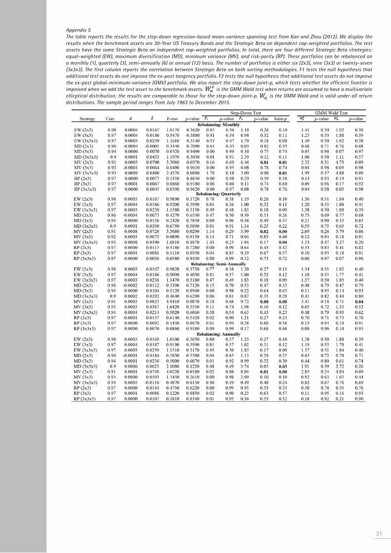
Appendix 5The table reports the results for the step-down regression-based mean-variance spanning test from Kan and Zhou (2012). We display the results when the benchmark assets are 30-Year US Treasury Bonds and the Strategic Beta on dependent cap-weighted portfolios. The test assets have the same Strategic Beta on independent cap-weighted portfolios. In total, there are four different Strategic Beta strategies: equal-weighted (EW), maximum diversification (MD), minimum variance (MV), and risk-parity (RP). These portfolios can be rebalanced on a monthly (1), quarterly (3), semi-annually (6) or annual (12) basis. The number of portfolios is either six (2x3), nine (3x3) or twenty-seven (3x3x3). The first column reports the correlation between Strategic Beta on both sorting methodologies. F1 tests the null hypothesis that additional test assets do not improve the ex-post tangency portfolio. F2 tests the null hypothesis that additional test assets do not improve the ex-post global-minimum-variance (GMV) portfolio. We also report the step-down joint-p, which tests whether the efficient frontier is improved when we add the test asset to the benchmark assets. is the GMM Wald test when returns are assumed to have a multivariate ellicptical distribution; the results are comparable to those for the step-down joint-p. is the GMM Wald and is valid under all return distributions. The sample period ranges from July 1963 to December 2015.

31

32

Appendix 6The table reports the results for the step-down regression-based mean-variance spanning test from Kan and Zhou (2012). We display the results when the benchmark assets are 30-Year US Treasury Bonds and the Strategic Beta on dependent equally weighted portfolios. The test assets have the same Strategic Beta on independent equally weighted portfolios. In total, there are four different Strategic Beta strategies: equal-weighted (EW), maximum diversification (MD), minimum variance (MV), and risk-parity (RP). These portfolios can be rebalanced on a monthly (1), quarterly (3), semi-annually (6) or annual (12) basis. The number of portfolios is either six (2x3), nine (3x3) or twenty-seven (3x3x3). The first column reports the correlation between Strategic Beta on both sorting methodologies. F1 tests the null hypothesis that additional test assets do not improve the ex-post tangency portfolio. F2 tests the null hypothesis that additional test assets do not improve the ex-post global-minimum-variance (GMV) portfolio. We also report the step-down joint-p, which tests whether the efficient frontier is improved when we add the test asset to the benchmark assets. is the GMM Wald test when returns are assumed to have a multivariate elliptical distribution; the results are comparable to those for the step-down joint-p. is the GMM Wald and is valid under all return distributions. The sample period ranges from July 1963 to December 2015.

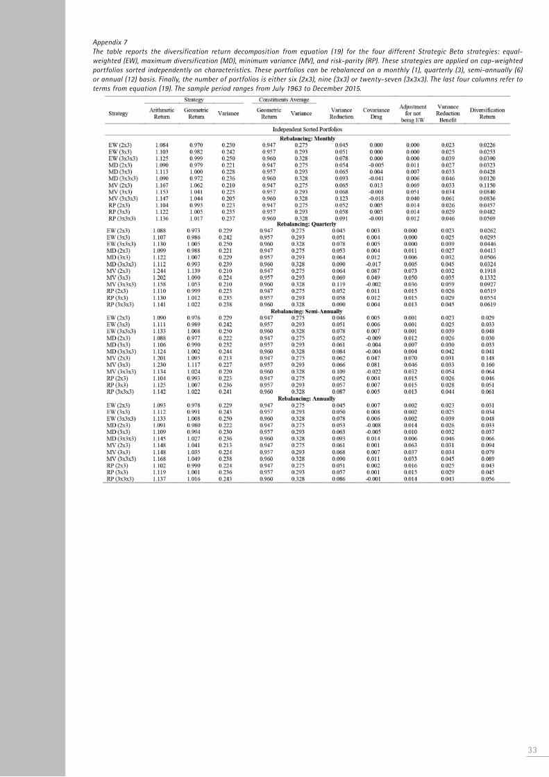
Appendix 7The table reports the diversification return decomposition from equation (19) for the four different Strategic Beta strategies: equal-weighted (EW), maximum diversification (MD), minimum variance (MV), and risk-parity (RP). These strategies are applied on cap-weighted portfolios sorted independently on characteristics. These portfolios can be rebalanced on a monthly (1), quarterly (3), semi-annually (6) or annual (12) basis. Finally, the number of portfolios is either six (2x3), nine (3x3) or twenty-seven (3x3x3). The last four columns refer to terms from equation (19). The sample period ranges from July 1963 to December 2015.

33

34

Appendix 8The table reports the diversification return decomposition from equation (19) for the four different Strategic Beta strategies: equal-weighted (EW), maximum diversification (MD), minimum variance (MV), and risk-parity (RP). These strategies are applied on equal-weighted portfolios sorted independently on characteristics. These portfolios can be rebalanced on a monthly (1), quarterly (3), semi-annually (6) or annual (12) basis. Finally, the number of portfolios is either six (2x3), nine (3x3) or twenty-seven (3x3x3). The last four columns refer to terms from equation (19). The sample period ranges from July 1963 to December 2015.

Appendix 9The table reports the diversification return decomposition from equation (19) for the four different Strategic Beta strategies: equal-weighted (EW), maximum diversification (MD), minimum variance (MV), and risk-parity (RP). These strategies are applied on cap-weighted portfolios sorted dependently on characteristics. These portfolios can be rebalanced on a monthly (1), quarterly (3), semi-annually (6) or annual (12) basis. Finally, the number of portfolios is either six (2x3), nine (3x3) or twenty-seven (3x3x3). The last four columns refer to terms from equation (19). The sample period ranges from July 1963 to December 2015.

35

36

Appendix 10The table reports the diversification return decomposition from equation (19) for the four different Strategic Beta strategies: equal-weighted (EW), maximum diversification (MD), minimum variance (MV), and risk-parity (RP). These strategies are applied on equal-weighted portfolios sorted dependently on characteristics. These portfolios can be rebalanced on a monthly (1), quarterly (3), semi-annually (6) or annual (12) basis. Finally, the number of portfolios is either six (2x3), nine (3x3) or twenty-seven (3x3x3). The last four columns refer to terms from equation (19). The sample period ranges from July 1963 to December 2015.

References• Ardia, D., K. Boudt, and G. Nguyen. “Beyond Risk-Based Portfolios : Balancing Performance and Risk Contributions in Asset Allocation.” Working Paper (2017), University of Neuchâtel.

• Amenc, N.; F. Goltz; and A. Lodh. "Smart Beta is Not Monkey Business." The Journal of Index Investing, 6 (2016), 12–29.

• Amenc, N.; F. Goltz; A. Lodh; and L. Martellini. "Towards Smart Equity Factor Indices:Harvesting Risk Premia without Taking Unrewarded Risks." The Journal of Portfolio Management, 40 (2014), 106–122.

• Amenc, N.; F. Goltz; and L. Martellini. "Smart Beta 2.0." Working Paper, EDHEC Risk Institute, (2013), 83–99.

• Arnott, R. .D, J. Hsu, V. Kalesnik, and P. Tindall. “The Surprising Alpha from Malkiel’s Monkey and Upside-Down Strategies.” The Journal of Portfolio Management 39 (2013): 91–105.

• Arnott, R. D., J. Hsu, and P. Moore. “Fundamental Indexation.” Financial Analysts Journal 61 (2005), 83–99.

• Asness, C. S.; A. Frazzini; and L. H. Pedersen. "Leverage Aversion and Risk Parity." Financial Analysts Journal, 68 (2012), 47–59.

• Baker, M.; B. Bradley; and R. Taliaferro. "The Low-Risk Anomaly: A Decomposition into Micro and Macro Effects." Financial Analysts Journal, 70 (2014), 43–58.

• Barberis, N., and A. Shleifer. "Style Investing." Journal of Financial Economics, 68 (2003), 161–199.

• Barberis, N., A. Shleifer, and J. Wurgler. “Comovement.” Journal of Financial Economics 75 (2005), 283–317.

• Bera, A. K, and S. Y Park. “Optimal Portfolio Diversification Using the Maximum Entropy Principle.” Econometric Reviews 27 (2008): 484–512.

• Berk, J. B. "Sorting Out Sorts." The Journal of Finance, 55 (2000), 407–427.

• Booth, D. G., and E. F. Fama. "Diversification Returns and Asset Contributions." Financial Analysts Journal, 48 (1992), 26–32.

• Bouchey, P.; N. Vassilii; A. Paulsen; and D. M. Stein. “Volatility Harvesting : Why Does Diversifying and Rebalancing Create Portfolio Growth?” The Journal of Wealth Management 15 (2012), 26–35.

• Boudt, K., and P. Benedict. "Smart Harvesting of Equity Style Premia." Working Paper, Vrije Universiteit Brussel (2013), 1–18.

• Carhart, M. M. "On Persistence in Mutual Fund Performance." The Journal of Finance, 52 (1997), 57–82.

• Chaves, D.; J. Hsu; F. Li; and O. Shakernia. "Risk Parity Portfolio vs. Other Asset Allocation Heuristic Portfolios." The Journal of Investing, 20 (2011), 108–118.

• Chaves, D.; J. Hsu; F. Li; and O. Shakernia. “Efficient Algorithms for Computing Risk Parity Portfolio Weights.” Journal of Investing 21 (2012), 150–63.

• Chen, H.-C.; K.-Y. Ho; and C.-H. Wu. "Initial Public Offerings: An Asset Allocation Perspective." Working Paper, (2004), 45.

• Chen, W.-P.; H. Chung; K.-Y. Ho; and T.-L. Hsu. "Portfolio Optimisation Models and Mean–Variance Spanning Tests." In Handbook of Quantitative Finance and Risk Management, (2010), 168–184.

• Choueifaty, Y., and Y. Coignard. "Toward Maximum Diversification." The Journal of Portfolio Management, 35 (2008), 40–51.

• Clarke, R.; H. D. Silva; and S. Thorley. "Risk Parity, Maximum Diversification, and Minimum Variance:An Analytic Perspective." The Journal of Portfolio Management, 39 (2013), 39–53.

37

38

• Daniel, K.; M. Grinblatt; S. Titman; and R. Wermers. "Measuring Mutual Fund Performance with Characteristic-Based Benchmarks." The Journal of Finance, 52 (1997), 1035–1058.

• DeMiguel, V.; L. Garlappi; and R. Uppal. "Optimal Versus Naive Diversification: How Inefficient is the 1/N Portfolio Strategy?" Review of Financial Studies, 22 (2009), 1915–1953.

• Elton, E. J., and M. J. Gruber. "Estimating the Dependence Structure of Share Prices--Implications for Portfolio Selection." The Journal of Finance, 28 (1973), 1203–1232.

• Erb, C. B., and C. R. Harvey. "The Strategic and Tactical Value of Commodity Futures." Financial Analysts Journal, 62 (2006), 69–97.

• Fama, E. F., and K. R. French. "Common Risk Factors in the Returns on Stocks and Bonds." Journal of Financial Economics, 33 (1993), 3–56.

• Fisher, G. S.; P. Z. Maymin; and Z. G. Maymin. "Risk Parity Optimality." The Journal of Portfolio Management, 41 (2015), 42–56.

• Frazzini, A., and L. H. Pedersen. "Betting Against Beta." Journal of Financial Economics, 111 (2014), 1–25.

• Froot, K., and M. Teo. "Style Investing and Institutional Investors." Journal of Financial and Quantitative Analysis, 43 (2008), 883–906.

• Graham, Jeffrey. "Comment on the Theoretical and Empirical Evidence of Fundamental Indexing." Journal of Investment Management 10 (2012), 90- 98

• Gorton, G. B., and G. K. Rouwenhorst. "A Note on Erb and Harvey (2005)." Working Paper, Yale School of Management (2006).

• Hasbrouck, J. "Trading Costs and Returns for U.S. Equities: Estimating Effective Costs from Daily Data." The Journal of Finance, 64 (2009), 1445–1477.

• Hsu, J. “Cap-Weighted Portfolios Are Sub-Optimal Portfolios.” Journal of Investment Management 4 (2006), 44–53.

• Hsu, J., and V. Kalesnik. "Measuring the ‘Skill’ of Index Portfolios." Working Paper, UCLA Anderson School of Management (2014).

• Huberman, G., and S. Kandel. “Mean-Variance Spanning.” The Journal of Finance 42 (1987): 873–88.

• Idzorek, T. M., and M. Kowara. “Factor-Based Asset Allocation vs. Asset-Class-Based Asset Allocation.” Financial Analysts Journal 69 (2013), 19–29.

• Jun, D., and B. G. Malkiel. “New Paradigms in Stock Market Indexing.” European Financial Management 14 (2007), 118–26.

• Kan, R., and G. Zhou. "Tests of Mean-Variance Spanning." Annals of Economics & Finance, 13 (2012), 139–187.

• Lambert, M., B. Fays; and G. Hübner. "Size and Value Matter, But Not The Way You Thought." Working Paper, University of Liege, HEC Liege (2016).

• Lambert, M., and G. Hübner. "Comoment Risk and Stock Returns." Journal of Empirical Finance, 23 (2013), 191–205.

• Ledoit, O., and M. Wolf. "A Well-Conditioned Estimator for Large-Dimensional Covariance Matrices." Journal of Multivariate Analysis, 88 (2004), 365–411.

• Lintner, J. "Security Prices, Risk, and Maximal Gains from Diversification." The Journal of Finance, 20 (1965), 587–615.

• Maillard, S.; T. Roncalli; and J. Teïletche. "The Properties of Equally Weighted Risk Contribution Portfolios." The Journal of Portfolio Management, 36 (2010), 60–70.

• Malkiel, B. G. "Is Smart Beta Really Smart?" The Journal of Portfolio Management, 40 (2014), 127–134.

• Markowitz, H. "Portfolio Selection." The Journal of Finance, 7 (1952), 77–91.

• Markowitz, H. M. "Market Efficiency: A Theoretical Distinction and So What?" Financial Analysts Journal, 61 (2005), 17–30.

• Marshall, B. R., N. H. Nguyen, and N. Visaltanachoti. "Commodity Liquidity Measurement and Transaction Costs." Review of Financial Studies, 25 (2011), 599–638.

• Mossin, J. "Equilibrium in a Capital Asset Market." Econometrica, 34 (1966), 768–783.

• Novy-Marx, R. "The Other Side of Value: The Gross Profitability Premium." Journal of Financial Economics, 108 (2013), 1–28.

• Novy-Marx, R., and M. Velikov. "A taxonomy of anomalies and their trading costs." The Review of Financial Studies, 29 (2016), 104–147.

• Patton, A. J., and A. Timmermann. "Monotonicity in Asset Returns: New Tests with Applications to the Term Structure, the CAPM, and Portfolio Sorts." Journal of Financial Economics, 98 (2010), 605–625.

• Perold, A. F. “Fundamentally Flawed Indexing.” Financial Analysts Journal 63 (2007): 31–37.

• Plyakha, Y., U. Raman, and V. Grigory. "Equal or Value Weighting ? Implications for Asset-Pricing Tests." Working Paper, University of Luxembourg (2014).

• Plyakha, Y., R. Uppal, and G. Vilkov. "Why Do Equal-Weighted Portfolios Outperform Value-Weighted Portfolios?" Working Paper, University of Luxembourg (2015).

• Podkaminer, E. "The Education of Beta: Can Alternative Indexes Make Your Portfolio Smarter?" The Journal of Investing, 24 (2015), 7–34.

• Qian, E. "Risk Parity and Diversification." The Journal of Investing, 20 (2011), 119–127.

• Roll, R. "A Simple Implicit Measure of the Effective Bid-Ask Spread in an Efficient Market." The Journal of Finance, 39 (1984), 1127–1139.

• Roncalli, T., and G. Weisang. “Risk Parity Portfolios with Risk Factors.” Quantitative Finance 16 (2016): 377–88.

• Sharpe, W. F. "Capital Asset Prices: A Theory of Market Equilibrium under Conditions of Risk." The Journal of Finance, 19 (1964), 425–442.

• Sharpe, W. F. "The Arithmetic of Active Management." Financial Analysts Journal, 47 (1991), 7–9.

• Steiner, A. "Risk Parity for the Masses." The Journal of Investing, 21 (2012), 129–139.

• Tobin, J. “Liquidity Preference as Behaviour Towards Risk.” The Review of Economic Studies 25 (1958), 65–86.

• Wahal, S., and M. D. Yavuz. "Style Investing, Comovement and Return Predictability." Journal of Financial Economics, 107 (2013), 136–154.

• Willenbrock, S. "Diversification Return, Portfolio Rebalancing, and the Commodity Return Puzzle." Financial Analysts Journal, 67 (2011), 42–49.

39

Founded in 1906, EDHEC Business School offers management education at undergraduate, graduate, post-graduate and executive levels. Holding the AACSB, AMBA and EQUIS accreditations and regularly ranked among Europe’s leading institutions, EDHEC Business School delivers degree courses to over 6,000 students from the world over and trains 5,500 professionals yearly through executive courses and research events. The School’s ‘Research for Business’ policy focuses on issues that correspond to genuine industry and community expectations.

Established in 2001, EDHEC-Risk Institute has become the premier academic centre for industry-relevant financial research. In partnership with large financial institutions, its team of ninety permanent professors, engineers, and support staff, and forty-eight research associates and affiliate professors, implements six research programmes and sixteen research chairs and strategic research

projects focusing on asset allocation and risk management. EDHEC-Risk Institute also has highly significant executive education activities for professionals.

In 2012, EDHEC-Risk Institute signed two strategic partnership agreements with the Operations Research and Financial Engineering department of Princeton University to set up a joint research programme in the area of risk and investment management, and with Yale School of Management to set up joint certified executive training courses in North America and Europe in the area of investment management.

In 2012, EDHEC-Risk Institute set up ERI Scientific Beta, which is an initiative that is aimed at transferring the results of its equity research to professionals in the form of smart beta indices.

Copyright © 2018 EDHEC-Risk Institute

EDHEC-Risk Institute393 promenade des AnglaisBP 3116 - 06202 Nice Cedex 3FranceTel: +33 (0)4 93 18 78 87

EDHEC Risk Institute—Europe 10 Fleet Place, LudgateLondon EC4M 7RBUnited KingdomTel: +44 207 3325600

https://risk.edhec.edu

For more information, please contact: Maud Gauchon on +33 (0)4 93 18 78 87 or by e-mail to: maud.gauchon@edhec-risk.com