Smart Money? The Effect of Education on Financial Outcomes

Shawn Cole, Anna Paulson, and Gauri Kartini Shastry1

August 2013

Abstract

Household financial decisions are important for household welfare, economic growth and financial stability. Yet, our understanding of the determinants of financial decision-making is limited. Exploiting exogenous variation in state compulsory schooling laws in both standard and two-sample instrumental variable strategies, we show education increases financial market participation, measured by investment income and equities ownership, while dramatically reducing the probability that an individual declares bankruptcy, experiences a foreclosure, or is delinquent on a loan. Further results and a simple calibration suggest the result is driven by changes in savings or investment behavior, rather than simply increased labor earnings.

1 Harvard Business School (scole@hbs.edu) and National Bureau of Economic Research, Federal Reserve Bank of Chicago (anna.paulson@chi.frb.org), and Wellesley College (gshastry@wellesley.edu), respectively. We thank the editor, an anonymous referee, and Josh Angrist, Malcolm Baker, Daniel Bergstresser, Carol Bertaut, David Cutler, Robin Greenwood, Campbell Harvey, Caroline Hoxby, Michael Kremer, Annamaria Lusardi, Erik Stafford, Jeremy Tobacman, Petia Topalova, Peter Tufano, and workshop participants at Harvard, the Federal Reserve Board of Governors, the University of Virginia, Wellesley College, the American Economic Association, the University of Connecticut and the Federal Reserve Bank of Boston for comments and suggestions. Paymon Khorrami, Wentao Xiong, Caitlin Kearns, and Veronica Postal provided excellent research assistance. The views presented in this paper are those of the authors and do not necessarily reflect those of the Federal Reserve Bank of Chicago.

1

Smart Money? The Effect of Education on Financial Outcomes

August 2013

Abstract

Household financial decisions are important for household welfare, economic growth and financial stability. Yet, our understanding of the determinants of financial decision-making is limited. Exploiting exogenous variation in state compulsory schooling laws in both standard and two-sample instrumental variable strategies, we show education increases financial market participation, measured by investment income and equities ownership, while dramatically reducing the probability that an individual declares bankruptcy, experiences a foreclosure, or is delinquent on a loan. Further results and a simple calibration suggest the result is driven by changes in savings or investment behavior, rather than simply increased labor earnings.

2

1 Introduction

Individuals face an increasingly complex set of financial decisions. On the asset side of

the balance sheet, the shift to defined contribution pension plans and the growing importance of

private retirement accounts require individuals to choose the amount they save, as well as the

mix of assets in which they invest. On the liability side, a dramatic increase in the range and

complexity of credit products available to households has been accompanied by increased

default, bankruptcy, and foreclosures. In May 2013, only 46% of non-retired Americans reported

that they expected to have enough money to support a “comfortable retirement.”2 These facts,

along with the recent financial crisis, have sparked a vigorous debate about whether individuals

are well-equipped to make informed financial decisions. For example, the director of the

Consumer Financial Protection Bureau has testified that “education is the cornerstone” for the

capability of managing financial affairs3, and several mortgage lenders have admitted to steering

borrowers with low levels of education towards unattractive (but profitable) mortgages.4 Yet to

date, we have only a limited understanding of what factors affect financial market participation

and responsible use of credit.

Using data and estimation techniques new to the literature, this paper provides precise,

causal estimates of the effect of education on financial market participation, income from

investments in financial instruments, and credit management. Previous work has established a

strong correlation between education and financial outcomes, but to date, there has been no

measure of a causal relationship. Education and financial market outcomes may be correlated

with unobservable characteristics (such as ability or family background), causing potentially 2 Gallup Poll, May 2013, http://www.gallup.com/poll/162842/americans-optimistic-comfortable-retirement.aspx, accessed June 2013. 3 http://www.consumerfinance.gov/speeches/prepared-remarks-of-richard-cordray-at-the-federal-reserve-bank-of-chicago-visa-inc-financial-literacy-and-education-summit/, accessed August 2013. 4 Kristof, Nicholas, New York Times, 11/30/2010.

3

spurious correlation. It is also important for policymakers to have a precise causal estimate, so

they can understand better how the changing educational environment may affect financial

outcomes.

To estimate a causal effect, we exploit exogenous variation in education caused by

changes in compulsory schooling laws. In our preferred specification, using a sample of U.S.

Census data for almost 15 million individuals, we find that an additional year of education

increases the probability that an individual has any non-zero investment income by 7-8

percentage points, holding other factors, including labor market income, constant. Using a

second dataset, we find that an additional year of education increases the probability of owning

equities by 4 percentage points. The size of this effect is economically important both on its own

and in the context of previously identified correlates of financial participation, such as trust

(Guiso, Sapienza, and Zingales, 2008), peer effects (Hong, Kubik, and Stein, 2004), prior stock

market experience (Malmendier and Nagel, 2011), or institutional quality (Osili and Paulson,

2008).

To study the effect of education on financial outcomes beyond simple participation in

financial markets, we implement a two-sample instrumental variables strategy, combining

Census data with a new dataset, the Federal Reserve Bank of New York Consumer Credit

Panel/Equifax dataset. We find that exogenous increases in education lead to substantial

reductions in the probability of bankruptcy and foreclosure, slightly higher credit scores, and

fewer delinquent credit-card payments. The effect of education on foreclosure was particularly

pronounced during the recent financial crisis.

Establishing a causal link between education and financial outcomes is a key contribution

of this paper, and it is important to be clear about what our identification strategy estimates. We

4

measure a “Local Average Treatment Effect (LATE),” that is, the effect of additional education

on financial outcomes for the set of individuals whose ultimate educational attainment was

altered by changes in compulsory schooling laws. This group includes many individuals whose

financial situation is of concern to policymakers, namely the lower-income segment of the

population.5

The final portion of our paper explores the potential mechanisms by which education

affects financial outcomes. This is made difficult by the fact that we cannot observe commonly

studied financial behaviors, such as the alpha of individuals’ portfolios. One obvious channel is

that better educated individuals earn higher wages, enabling them to accumulate more assets and

earn additional investment income as a result. However, a simple back-of-the-envelope

calculation demonstrates that the estimated effect of education on the level of investment income

is too large to come solely from this wage return to education, without a concurrent change in

savings rates or investment decisions. This calibration, along with the finding that educated

people are more likely to participate in the stock market, accumulate any return-yielding assets,

and stay current with their credit card debt, suggests that education may improve financial

management and decision-making. We discuss support for this interpretation in Section 5.

This paper contributes to a growing literature on household finance. Much attention has

focused on three features of household behavior that may be inconsistent with standard models.

The first is the low level of participation in equity markets relative to the returns offered by

stocks: In 2004, only 48.6% of households held stocks, either directly or indirectly (Bucks,

Kennickell, and Moore, 2006). Haliassos and Bertaut (1995) consider and reject risk aversion,

belief heterogeneity, and other potential explanations for the limited participation puzzle, instead

5 Gallup Poll, May 2013, http://www.gallup.com/poll/162239/middle-aged-americans-worried-finances.aspx, accessed June 2013.

5

favoring departures from expected-utility maximization. Our paper shows that low levels of

education may help explain limited participation in equity markets.

A second “puzzle” to which our work relates is the apparently low savings rate of the

U.S. population, particularly among lower-income individuals. Lusardi et al. (2011) report that

only one-quarter of the U.S. population has the capacity to come up with $2,000 within 30 days

to meet an unexpected expense. Our results demonstrate that education dramatically affects

savings outcomes among more vulnerable population segments, specifically those on the margin

of completing high school.

Finally, researchers have been paying more attention to the possibility that behavioral

biases may cause consumers to choose the wrong credit products or borrow too much. For

example, Campbell et al. (2011) suggest that consumers make financial mistakes that result in

significant costs not only to themselves but to the stability of the financial system, and that this

behavior is correlated with low levels of education. Gross and Souleles (2002) note that

individuals borrow from credit cards, even when they hold large bank account balances.

While survey evidence has proven useful in demonstrating factors that are correlated with

such behaviors,6 there is much less understanding of what the causal drivers are. This paper

contributes to the literature by showing that variation in educational attainment across the U.S.

population can help to explain some of these puzzles.

More generally, the depth and breadth of financial market participation are thought to be

important in determining the equity premium, the volatility of markets, and household

expenditure (Mankiw and Zeldes, 1991; Heaton and Lucas, 1999; Vissing-Jorgensen, 2002; and

6 Previous work has demonstrated that financial behavior is, not surprisingly, correlated with income, education (Bertaut and Starr-McCluer, 2001, among others), measured financial literacy (Lusardi and Mitchell, 2007), social connections (Hong, Kubik, and Stein, 2004), trust (Guiso, Sapienza, and Zingales, 2008), experience with the stock market (Malmendier and Nagel, 2011), and cognitive ability (Grinblatt, Keloharju, and Linnainmaa, 2011).

6

Brav, Constantinides, and Gezcy, 2002). Financial behavior may also affect the political

economy of financial regulation, as those holding financial assets may have different attitudes

towards corporate and investment income tax policy, as well as risk-sharing and redistribution.

2 Data

This paper uses three complementary datasets: the U.S. Census, the Survey of Income

and Program Participation (SIPP), and the Federal Reserve Bank of New York Consumer Credit

Panel/Equifax dataset (FRBNY-CCP). Summary statistics are presented in Table 1.

2.1 The Census

We first use a 5 percent sample from the 1980, 1990, and 2000 Public Use Census Data,

representing a random draw of the U.S. population. The key advantage of this dataset is its size:

with over 14 million observations, we can use non-parametric controls, obtain precise estimates,

and, most importantly, use instrumental variable strategies that would not be possible with most

other, smaller, datasets.

The main limitation to using the Census is that it does not collect any information on

financial wealth. Because of this, the Census is not typically used to study financial behavior (an

exception is Carroll, Rhee and Rhee, 1999). However, the Census does collect detailed income

data, including income derived from investments. Thus, the main financial indicator we use from

the Census is “income from interest, dividends, net rental income, royalty income, or income

from estates and trusts,” received during the previous year, which we term “investment income.”

Note that investment income can be negative or positive and that households are instructed to

“report even small amounts credited to an account” (Ruggles et al., 2004). A second type of

income we use is “retirement, survivor, or disability pensions,” received during the previous

7

year, which we term “retirement income.” This is distinct from Social Security and Supplemental

Security Income, both of which are reported separately.

We note a number of limitations to using the amount of investment income received

without specific information on investment allocations. First, investment income is only partially

informative about the amount and type of investments held by the respondent. This would make

it difficult to rely on Census data for structural estimates of investment levels (such as calibrating

models of the cost of participating in financial markets, for example). In our analysis of the

Census data, however, we focus primarily on the decision to accumulate any return-yielding

assets, for which we define a dummy variable equal to one if the household reports any non-zero

investment income (positive or negative). Throughout the paper, we will refer to this outcome as

“any investment income.”7 Second, one may be concerned that small amounts of investment

income simply represent interest from savings accounts. As a robustness check, we rerun our

analysis defining participants as either: i) those who report investment losses or investment

income greater than $500; or ii) those who report investment losses or investment income above

a cut-off predicted using the savings account interest earnings from the Survey of Consumer

Finances (SCF) or SIPP. Third, it is possible that an individual may hold assets that do not yield

a return within the year, such as growth stocks or zero-coupon bonds. In our view it is unlikely

that such an individual would not also have a savings account that earned interest income.

Finally, unlike the SCF, the Census is not specifically aimed at measuring complex

financial information. Therefore, in Online Appendix Tables A1 and A2, we compare the Census

data with data from the SCF. We find that the Census data yield very similar estimates of means,

medians, and percentiles for our measures of participation, investment and retirement income.

7 In Online Appendix Table A6, we also examine whether individuals report negative investment income, but in the paper, the outcome we study is equal to one if an individual reports positive or negative investment income.

8

We also explore the relationship between reported investment income and more traditional

measures of financial market participation. In particular, we find a large jump in the use of

transactions accounts as individuals move from zero to any positive amount of investment

income. For example, 78% of households reporting no investment income possess a checking

account, while 92% of those reporting investment income between $1 and $100 have checking

accounts. There is a similar, strongly positive and nearly linear relationship between reported

investment income and participation in equity markets. Further details of this comparison are

described in the online data appendix.

2.2 The Survey of Income and Program Participation (SIPP)

We complement the binary measure of any investment income from the Census with data

from a second source: direct data on equity ownership from the SIPP. The SIPP, conducted by

the Census Bureau, is a series of national panel surveys that began in 1984. We use all panels

from 1984 to 2008 to generate a sample size large enough to exploit the compulsory schooling

instrumental-variable strategy. Each panel is a nationally representative sample of 14,000-37,000

thousand households; households are surveyed every four months for four years. The survey is

built around a core set of demographic and income questions that include ownership of different

types of assets such as transaction accounts, stocks, bonds, and mutual funds.8 The SIPP has a

broader range of financial variables, and we employ it as a complement to the Census. Our

primary analysis focuses on the Census dataset, which provides a sample size fifty times larger

than that of the SIPP and, therefore, yields more precise estimates and greater confidence in the

8 Each survey wave also includes topical modules that gather additional information on assets and liabilities—for example, the monetary value of stocks and bonds—but these questions are not available in all years. Thus, the sample size falls substantially when we use these variables, rendering the instruments too weak for interpretation. For this reason, we focus on a binary measure of financial market participation, whether or not respondents own any equity, rather than the extent of their participation in financial markets.

9

validity of the instrumental variable strategy.

2.3 The FRBNY Consumer Credit Panel/Equifax dataset (FRBNY-CCP)

The FRBNY Consumer Credit Panel/Equifax dataset is a quarterly longitudinal panel of

individual credit bureau data, similar to information that would be contained in an individual's

credit report. It is described in detail in Lee and van der Klaauw (2010). The panel begins in the

first quarter of 1999, and we analyze data through the third quarter of 2011. The primary sample

is a random 5% sample of all U.S. residents aged 18 years or older who have a credit report. The

sample selection procedures ensure that, in any given quarter, there is a nationally representative

cross-section of individuals, conditional on having a credit report. We restrict attention to

individuals aged 36 to 75 in the third quarter of 2000, to match the Census sample. Ultimately,

the FRBNY-CCP dataset we analyze includes approximately five million individuals.

We focus on five key outcome variables from this dataset: a bankruptcy indicator, a

foreclosure indicator, a credit score, the proportion of an individual’s credit card debt that is not

delinquent, and the proportion of quarters in which an individual has any delinquent credit card

balance. The bankruptcy and foreclosure variables indicate whether an individual has undergone

bankruptcy or foreclosure at least once, respectively, between 1992 and 2011. These indicators

are able to track bankruptcies and foreclosures back through 1992 because credit bureaus

maintain records on these proceedings for seven years. The credit score, similar to a FICO score,

predicts the likelihood of being 90 or more days delinquent over the next 24 months. Credit

scores range from 280 to 850, and higher scores imply a lower probability of being seriously

delinquent in the future. Both the credit score and the proportion of an individual’s credit card

debt that is not delinquent are averaged across all quarters. We do this because even though there

is time-series variation in the outcome variables, the exogenous variation in education is cross-

10

sectional and does not vary at the individual level over time. Calculating averages is one way to

address potential serial correlation in the same individual’s credit scores and delinquency from

month to month (Angrist and Pischke, 2008).9

3 The Effect of Education on Asset Accumulation and Financial Market Participation

3.1 Empirical Strategy

While researchers have documented a positive correlation between educational

attainment and financial behavior (for example, Campbell (2006) notes educated households in

Sweden have more diversified portfolios), the literature has not produced credible estimates of

the causal effect of education on financial outcomes.10 Education and behavior are both likely to

be correlated with factors like ability, making it hard to isolate the causal impact of education

(Griliches, 1977).

To overcome this problem, we adopt an instrumental variables (IV) strategy first

developed in Acemoglu and Angrist (2000). We use changes in state compulsory education laws

as an instrument for educational attainment. This provides exogenous variation in education:

revisions to state laws affect individual educational attainment, but are not correlated with

individual ability, parental characteristics, or other potentially confounding factors.

In particular, we follow the strategy laid out by Lochner and Moretti (2004, hereafter

LM), who use changes in state schooling requirements to measure the effect of education on

incarceration rates. States revised compulsory schooling laws numerous times from 1914 to

9 The size of the dataset precludes using all of the data and clustering. 10 Most of the literature suggests a positive correlation between education and financial outcomes. At the same time, Tortorice (2012) finds that education only slightly reduces the likelihood that individuals make expectational errors regarding macroeconomic variables and that these errors affect buying attitudes and financial decisions.

11

1978, and not always in the direction of requiring additional schooling. We use data from the

1980, 1990, and 2000 Censuses and focus on individuals between 18 and 75 years old, who were

born in or before 1964.11 The principal advantage of following LM closely is that they have

conducted a battery of specification checks, demonstrating the validity of using compulsory

schooling laws as a natural experiment. For example, LM show that there is no clear trend in

educational attainment in the years prior to changes in schooling laws and that compulsory

schooling laws do not affect college attendance, supporting the identifying assumption that,

conditional on the controls (such as state and year of birth), the compulsory schooling laws in

effect when a student turned 14 are uncorrelated with omitted determinants of education or

financial outcomes. We provide evidence that these laws do influence at least some students to

acquire more schooling below, which is also necessary for the IV strategy to be valid.

The structural equation of interest is the following,

𝑦𝑖 = 𝛼 + 𝛽𝑠𝑖 + 𝛾𝑋𝑖 + 𝜀𝑖 (1)

where iy is a financial outcome for individual i, si is years of education for individual i, and Xi

is a set of controls that include age, gender, race, state of birth, state of residence, Census year,

cohort of birth fixed effects, and a cubic polynomial in earned income. The financial outcome

variable can be an indicator for having any investment or retirement income, the level of

investment or retirement income, or an indicator for whether the individual owns specific types

of assets (such as equity). When the outcome variable is the amount of investment or retirement

11LM use the 1960, 1970, and 1980 Censuses, which contain information on correctional facility residence and focus on a narrower age group, ages 20–60. The Census does not code a continuous measure of years of schooling, but rather identifies categories of educational attainment: preschool, grades 1–4, grades 5–8, grade 9, grade 10, grade 11, grade 12, 1–3 years of college, and college degree or more. We translate these categories into years of schooling by assigning each range of grades the highest number of years of schooling for that category. This should not affect our estimates, since individuals who fall within the ranges of grades 1–4, 5–8, and 1–3 years of college will not be influenced by the compulsory schooling laws that affect grades 9–12.

12

income, we drop top-coded or bottom-coded observations.12 We control for age through a series

of indicator variables for each three-year age group from 20 to 75, while year effects are

indicator variables for each Census year. We exclude people born in Alaska and Hawaii,13 but

include those born in the District of Columbia; thus we have 49 state-of-birth controls, but 51

state-of-residence controls. Again following LM, we include state-of-birth controls interacted

with an indicator variable equal to one for individuals born in the South who turned 14 in or after

1958 to allow for the impact of the Brown vs. Board of Education decision. A cohort of birth is

defined as a ten-year birth interval. Standard errors are corrected for intra-cluster correlation

within state of birth * year of birth.

As in Acemoglu and Angrist (2000) and LM, we create indicator variables for whether

the years of required schooling are eight or fewer, nine, ten, and 11 or more.14 These variables

are based on the law in place in an individual’s state of birth when the person turns 14 years of

age. As LM note, migration between birth and age 14 will add noise to this estimation, but the IV

strategy is still valid.15 The first stage for the IV strategy can then be written as

12 To preclude the possibility of revealing personal information, the Census “top-codes” values for individuals earning large amounts of investment income and “bottom-codes” values for individuals with large investment losses. Specifically, they replace the income variable for individuals with investment income above a year-specific limit with the median income of all individuals in that state earning above that limit and replace all losses in excess of a year-specific limit with the limit itself. Retirement income is top-coded similarly, but not bottom-coded. The percentage of top-coded and bottom-coded observations is very low: 0.48% are top-coded and 0.04% bottom-coded for investment income and 0.23% are top-coded for retirement income. Of course, using an indicator variable for any investment income as the dependent variable avoids this issue entirely. While Angrist and Pischke (2008, p.105-106) express concerns about IV Tobit, we nevertheless run Tobit regressions to account for top-coding, and find very similar results (available in the online appendix). Observations on investment income were bottom- or top-coded if they were outside the range of –$9,990 to $75,000 in 1980, –$9,999 to $40,000 in 1990 and –$10,000 to $50,000 in 2000. Observations on retirement income were top-coded if they were greater than $30,000 in 1990 and greater than $52,000 in 2000. The 1980 Census did not separate retirement income from other (non-investment) sources of income. We also drop all observations where these values were imputed. 13 This follows Lochner and Moretti (2004) and Acemoglu and Angrist (2000). Alaska and Hawaii did not become states until 1959, well after the first cohorts included in the analysis were born. 14 When states do not set the minimum required years of schooling, we define the years of mandated schooling as the difference between the latest age an individual is required to stay in school and the earliest age she is required to enroll. When these two measures disagree, we take the larger value. 15 In fact, even if we had state of high school attendance, we might prefer to use state of birth to avoid any endogeneity resulting from households who moved states as a response to education-related laws.

13

𝑠𝑖 = 𝛼 + 𝛿9𝐶𝑜𝑚𝑝9 + 𝛿10𝐶𝑜𝑚𝑝10 + 𝛿11𝐶𝑜𝑚𝑝11 + 𝛾𝑋𝑖 + 𝜀𝑖 (2)

where si is years of schooling, Comp9, Comp10, and Comp11 are indicator variables that specify

the required number of years of schooling that individual i was exposed to, and Xi is the same

set of controls defined above. (The omitted category is laws which required eight or fewer years

of schooling).

As discussed in the introduction, the estimates produced here are Local Average

Treatment Effects (LATE), which measure the effect of education on financial market

participation for those whose educational attainment was affected by changes in compulsory

education laws.16 We note that those who are in fact affected by the laws are likely to have low

levels of financial market participation and, thus, constitute a relevant study population. Using a

compulsory schooling reform that affected a large fraction of the United Kingdom’s population,

Oreopoulos (2006) finds a LATE estimate of the effect of education on earnings that is very

similar to the LATE estimated in the United States from a small fraction of the population.

3.2 Empirical Results

We begin, as is customary, with the naive OLS relationship between education and

participation (equation 1). These results match most closely what has been done in the previous

literature and serve as a useful point of reference, but are likely subject to omitted variable bias.

Panel A of Table 2 presents the OLS estimates using the Census data, while Panel B presents

estimates using SIPP data. In Panel A, the dependent variable is an indicator for any investment

income (Column 1) or any retirement income (Column 3) and the amount of investment or

retirement income (Columns 2 and 4, respectively). In Panel B, the dependent variable is an

indicator variable for whether the respondent has any transactions account (Column 1), bonds or 16 Imbens and Angrist (1994) provide a discussion of Local Average Treatment Effects.

14

government securities (Column 2), or stocks or mutual funds (Column 3). The OLS estimates

produce the expected positive correlation between education and financial market participation,

and the Census and SIPP estimates are comparable.

Before discussing the causal estimates from the IV estimation, we demonstrate the

validity of the first stage of our analysis and show that the compulsory schooling laws did, in

fact, influence educational attainment.17 In Table 3, we present the first stage regression of years

of schooling (Columns 1 and 3) or high school graduation (Columns 2 and 4) on the three

instrumental variables (Comp9, Comp10, and Comp11) and the controls discussed earlier.

Clearly, when states mandate a greater number of years of schooling, some individuals obtain

more education than they would have otherwise. Using Census data, requiring nine or ten years

of schooling is estimated to increase average years of completed education by approximately 0.2

years, while requiring 11 years of education is estimated to increase education by 0.27 years

(Column 1). Requiring students to remain in school for nine years of schooling increases their

probability of graduating high school by 3.9 percentage points (Column 2). Columns 3 and 4 use

the SIPP data to estimate the first stage and produce reassuringly similar estimates.18

Table 4 presents IV estimates of equation (1) for the impact of education on asset

accumulation and financial market participation. Panel A provides results using data from the

Census. Column 1 omits the cubic polynomial in earned income, since income could be affected

by education, and therefore captures the total causal effect of education on whether an individual

reports any investment income. An additional year of schooling increases the probability that an

17 Lochner and Moretti (2004) report a range of tests examining the exclusion restriction and demonstrate that the education mandates are not systematically correlated with other policies that might affect outcomes. 18 Weak instrument bias is not a problem in this context. We report the F-statistics of the excluded instruments in Tables 3 and 4. The F-statistics for the Census range from 37.7 to 52.4, well above the critical values proposed by Stock and Yogo (2005). The F-statistics for the SIPP are lower (due to the smaller sample size), but still within the range of appropriate critical values.

15

individual reports any investment income by 6.9 percentage points. Column 2 of Panel A

includes a cubic control for earned income (which includes wages and income from one’s own

business or farm).19 Although income itself may be affected by education, it is useful as a

specification check to examine whether the impact of education on financial outcomes is entirely

due to changes in earnings. In fact, we find that the point estimate on schooling is nearly

identical when we control for earned income in a flexible manner. This suggests that increased

income is not the only mechanism driving the result: education increases the probability of

accumulating any return-yielding assets, conditional on non-investment income. The striking fact

is that no matter how flexibly we control for earned income (such as with an earned income

spline, see Online Appendix Table A3), we find a persistent and large impact of education on

having any investment income.

In Columns 3–5, we consider the possibility that our measure of investment income

might simply reflect interest-bearing savings accounts, rather than a shift toward investment in

higher return financial products. We redefine the outcome variable in two ways. First, we define

a dummy equal to one if an individual has income from investments greater than $500 or any

losses, presuming that an individual whose only financial asset is a savings account would have

less than $500 in interest income and no losses. Columns 4 and 5 take this approach one step

further by using the detailed financial data in the SCF or the SIPP to predict an individual’s

savings account interest based on the individual’s age, earned income, race, sex, and either

19 Duflo et al. (2008, p. 3949) point out that including controls, such as income in our case, that may be affected by the experiment can lead to biased estimates. The Census dataset does not include any measures of wealth, but even if it did, we do not believe it would be an appropriate control. It also suffers from this econometric issue, but the problem is even worse for wealth than for income because wealth is, in fact, the outcome we care about. Accumulated wealth is the aggregation of years of past financial decisions regarding saving, investing, and borrowing; if we controlled for it, we would essentially be searching for an effect of education on this particular year’s financial outcomes, conditioning on a summary measure of all past financial outcomes.

16

survey year indicators or state of residence indicators, depending on data availability.20 The

outcome variable in these regressions is an indicator variable that is equal to one if an

individual’s investment income as reported in the Census surpasses the threshold estimated from

the second dataset or is negative.

In Column 6, we study the amount of income from investments and find a large and

significant effect of education. The magnitude is substantial: an additional year of schooling

increases investment income by $1,760.21 Finally, Columns 7 and 8 estimate the impact of

education on retirement income. An additional year of schooling increases the probability of

having any retirement income by 5.9 percentage points, and the amount of retirement income by

$966. The estimates are somewhat larger than the naive OLS estimates presented in Table 2,

suggesting that the OLS estimates produce a downward bias in the impact of schooling on

financial outcomes. We find similar effects when we use high school completion as the measure

of schooling (see Online Appendix Table A5).

Panel B of Table 4 presents IV estimates of the effect of years of schooling on financial

market participation using SIPP data. The first two columns show that education does not have a

statistically significant impact on whether or not an individual has a transactions account,

regardless of whether we control for a cubic polynomial in earned income. Columns 3–6

demonstrate that the positive relationship between years of schooling and ownership of bonds,

government securities, stocks, or mutual funds persists even after addressing the omitted variable

bias (with the instrumental variable strategy) and conditioning flexibly for non-investment

earnings. Note that the F-statistics of the excluded instruments are just strong enough (8.4–11.5)

to satisfy the “non-weak” instrument criteria established by Stock and Yogo (2005).

20 We thank an anonymous referee for this suggestion. 21 Using IV Tobit for investment income yields very similar results; results are in Online Appendix Table A4.

17

Unfortunately, data coverage for the value of assets held in these accounts is very often missing

(the SIPP did not ask for this information every year), so we are not able to report estimates for

the level of asset holdings using the SIPP data.

Looking at general ownership levels, we find that one more year of schooling increases

the likelihood that an individual owns any bonds or government securities by about 6.5

percentage points, and any stocks or mutual funds by 4 percentage points (p-value .06). These

magnitudes are close to those in Panel A Columns 1–3, supporting our interpretation of any

investment income as a measure of financial market participation. This interpretation receives

further support from the finding that increased education does not seem to increase transaction

account ownership, but does increase ownership of higher yielding investments. The “any

investment income” measure from the Census appears to be a useful proxy for broader financial

market participation.

The point estimates of the causal impact of education suggest that it is a very important

determinant of financial market participation. A convenient metric to compare the relative

importance across different studies is the effect size, which is the effect of a one standard

deviation change in the independent variable on participation. The effect size of education on

any investment income is about 19 percentage points, and the effect size of education on having

bonds or government securities and stocks or mutual funds is about 11 percentage points. The

magnitudes of these effects are larger than the magnitudes of trust (4 percentage points (Guiso,

Sapienza, and Zingales, 2008)) peer effects (4 percentage points (Hong et al., 2004)) of 1.15

percentage points, and experience with stock market returns (4.2 percentage points, (Malmendier

and Nagel, 2011)).

Three studies of retirement savings plan participation, serve as additional benchmarks for

18

evaluating the quantitative importance of education for financial outcomes. Duflo and Saez

(2003) present evidence from a randomized evaluation that minor incentives ($20 for university

staff attending a benefits fair) can increase retirement plan participation rates by 1.25 percentage

points. Duflo et al. (2006) offered low-income tax filers randomly assigned levels of IRA

contribution matches. They find that an offer of a 50 percent match increased IRA participation

by 14 percentage points, which is comparable to two years of education in our analysis.

However, no determinants of retirement plan participation have been found to be more effective

than simply changing the default enrollment status for 401(k) plans. Beshears et al. (2006) find

changing the default to enroll, increases participation by as much as 35 percentage points.

Taken together, using a credible identification strategy with two different datasets, these

results present a consistent picture: more education causes households to be more likely to invest

in high-return assets, such as equities, and to report higher levels of financial income.

4 Education and Credit Management

4.1 Empirical Strategy

Our analysis of the effects of education on credit management is complicated by the fact

that the credit bureau data do not have information on the key right-hand-side variable,

education, rendering standard OLS and IV estimation impossible. We take two approaches to

deal with this problem. First, we estimate the reduced-form relationship between compulsory

schooling laws and credit management as represented by the following equation:

𝑦𝑖 = 𝛼 + 𝛽9𝐶𝑜𝑚𝑝9 + 𝛽10𝐶𝑜𝑚𝑝10 + 𝛽11𝐶𝑜𝑚𝑝11 + 𝛾𝑋𝑖 + 𝜀𝑖, (3)

where 𝑦𝑖 is a credit management outcome, and Comp9, Comp10, and Comp11 are dummy

variables for the number of years an individual was required to attend school. The vector Xi

19

includes control variables that are similar to the ones used in the analysis of the SIPP and Census

datasets. Because the credit bureau data do not contain information on race, gender, or income,

these variables are omitted. The credit bureau does, however, include the zip code where an

individual lives, and we use zip-code-level fixed effects to control for income and other sources

of heterogeneity in some specifications.

The coefficients β9, β10, and β11 represent the effect of additional years of compulsory

schooling on credit outcomes, which is the policy-relevant effect of the compulsory schooling

laws. Since we have already shown that there is a strong positive relationship between these

compulsory schooling variables and education (see Table 3), we can infer a lot about the

relationship between education and credit outcomes from the estimated coefficients in equation

(3). For example, if Comp9 – Comp11 are positively related to an individual’s credit score, we

can infer that education is positively related to an individual’s credit score. We also estimate a

variation on equation (3) in which Comp9 – Comp11 are represented as a single variable equal to

the number of years an individual was required to attend school.

While the reduced-form strategy is easy to interpret and of interest for policy because it

captures the impact of compulsory schooling law changes on the population, it does not provide

a sense of the magnitude of the structural parameter of interest and is not comparable to the

LATE estimates discussed earlier. To produce comparable estimates of the causal effect of

education on credit outcomes, we take a two-sample instrumental variables approach, following

Angrist (1990).22 This strategy requires only that the instrumental variables and other right-hand-

side variables are available in both datasets, a requirement that is satisfied by the Census and

credit bureau dataset because they both contain information necessary to create the instrumental

22 Two-sample IV is relatively rare in the finance literature, but is used in Bitler, Moskowitz, and Vissing-Jorgensen (2005). We thank the editor for this suggestion.

20

variables: state of birth and year of birth.23

Specifically, we use the Census data to produce the first stage regression of education on

compulsory schooling (equation [2], similar to the results presented in Column [1] of Table 3,

except that the sample is restricted to data from the 2000 Census, so that it is aligned with the

credit bureau data). Since all the variables used to predict years of schooling are available in both

Census and credit bureau data, we then use the point estimates from this regression to create a

“predicted” level of education for each individual in the credit bureau data. Finally, we regress

the credit outcomes of interest on this predicted level of education. The only complication is in

how to correct standard errors for the fact that the right-hand-side variable is predicted. We

estimate standard errors in two ways. First, we provide robust standard errors, as described by

Murphy and Topel (1985). Second, we use a block bootstrap technique to generate a distribution

for the point estimate and use the standard deviation of this distribution for hypothesis testing.24

4.2 Empirical Results

We begin by discussing the reduced-form estimates of the effect of compulsory education

on credit management (equation [3]). These estimates are presented in Table 5. The outcomes

we examine are the probability of filing for bankruptcy or experiencing a foreclosure, credit

scores, the fraction of a borrower’s credit balance that is non-delinquent (averaged over the

period that is covered by the data, 1999–2011) and the fraction of quarters that a borrower has

any delinquent credit. Columns 1 through 3 of Panel A present evidence that compulsory

schooling laws reduce the probability that an individual declares bankruptcy. Cohorts who are

23 We use state of residence in the first quarter of the credit bureau panel to proxy for state of birth, because the FRBNY CCP/Equifax data do not include state of birth. Migration between birth and this date will add noise and make it more difficult to find an effect of education on credit management outcomes. 24 For a more detailed discussion of the two-sample instrumental variables technique, please see section 4.4 of Angrist and Pischke (2008).

21

required to attend school through the 11th grade have a 0.98 percentage point lower probability of

declaring bankruptcy than cohorts not required to attend school beyond the 8th grade. The

compulsory attendance dummies are jointly significant at the 1 percent level. Using years of

schooling required (Column 2) yields an estimate that each additional year of required schooling

reduces the probability of bankruptcy by 0.2 percentage points, significant at the 1 percent level.

Column 3 adds zip-code fixed effects, which control for geographic heterogeneity at a very fine

level (there are approximately 43,000 zip codes in the U.S.). Given the limitations of the credit

bureau data, the inclusion of zip-code fixed effects is as close as we can come to controlling for

income. The point estimate remains similar in magnitude and still significant.

Columns 4–6 study the effect of compulsory schooling on the probability that a

household experiences a foreclosure. Relative to those who were able to drop out before 9th

grade, cohorts in states that required attendance through the 11th grade were 1.2 percentage points

less likely to experience a foreclosure. Finally, Table 5, Panel B, Columns 1–9 examine the

reduced-form relationship between compulsory education laws and credit management, studying

the credit score, the fraction of borrower balance that is non-delinquent (averaged over the period

for which we have credit bureau data, 1999–2011) and the fraction of quarters a borrower has

any delinquent credit. We find statistically significant effects on all three outcomes, but they are

small in magnitude. Each year of required schooling increases credit scores by 0.253 points,

increases the percentage of borrower balance that is current by 0.02 percentage points, and

reduces the percentage of quarters delinquent by 0.03 percentage points. Note that it is not

surprising that these effects are small: These are the effects of an additional year of required

schooling, not an additional year of actual schooling. For many individuals, an additional year of

required schooling will have no effect on actual schooling. The reduced-form results provide the

22

average effect on the entire exposed cohort, including those for whom the change in compulsory

schooling laws did not change their eventual years of education.

We are also interested in the structural effect of an additional year of schooling on

individuals whose educational attainment was affected by the law. We use an instrumental

variable strategy to explore this. As described above, we use a two-sample IV approach, since

education levels are not available in the credit bureau data. The results are presented in Table 6.

Panel A presents estimates using the entire time period from the first quarter of 1999 to the last

quarter of 2011, while Panel B divides the data into pre- and post-financial-crisis periods. Within

each panel, the top results are estimates of equation (1) using the predicted level of education as

the key independent variable and using Murphy and Topel (1985) standard errors. The bottom

two rows of each panel repeat the same estimates using the standard deviation of the block

bootstrapped point estimates as the standard error.

The results suggest that education has important causal effects on credit outcomes. The

point estimate on the coefficient for years of schooling in Column 1, –0.033, is significant at the

1 percent level using Murphy and Topel standard errors, suggesting that an additional year of

schooling would reduce the probability of declaring bankruptcy by 3.3 percentage points. This

result is not significant when we use block-bootstrapped standard errors. In Column 2, we see

that an additional year of schooling is estimated to reduce the probability of experiencing

foreclosure by 5.7 percentage points, and this result is statistically significant at the 1 percent

level using either Murphy and Topel standard errors or the bootstrap. These effects are strikingly

large, especially relative to the population mean. Over the 1992 to 2011 period, 14.4% of

individuals declare bankruptcy, and 5.8% experience at least one foreclosure. However, it is

important to note two things. First, because these outcomes are particularly bad outcomes, they

23

may be especially relevant for the group of individuals whose education was affected by changes

in compulsory schooling laws. It is possible that the LATE is larger than the effect of education

on the average individual for credit management outcomes. This is in contrast to estimates of the

impact of education on income where LATE estimates are similar to the population parameters.

Second, standard confidence intervals include smaller effects as well: as small as 1.1 percentage

points for bankruptcy and 2.2 percentage points for foreclosure.

Estimates of the causal impact of education on other aspects of credit management are

somewhat smaller. A one standard deviation increase in education (2.7 years) would raise an

individual’s credit score by 20 points, increase the fraction of credit card balances kept current

by 1.4 percentage points relative to an unconditional average of 95.6%, and reduce the

percentage of quarters delinquent by 3.5 percentage points from a mean of 7.5 percentage points.

A 20-point movement in the credit score is less than one standard deviation in credit score.

However, there are certainly ranges where such perturbations can be very important. For

example, Chomsisengphet and Pennington-Cross (2006) document how a 20-point difference in

credit score can affect both the cost and availability of certain home mortgage products.

In Panel B of Table 6, we analyze whether the impact of education on bankruptcy and

foreclosure differs before and during the recent financial crisis. In Column 1, the dependent

variable is whether the individual declared bankruptcy between the second quarter of 1999 and

the third quarter of 2007, conditional on not having declared bankruptcy in the seven years prior

to 1999. In Column 3, the dependent variable is equal to one if the individual declared

bankruptcy between the third quarter of 2007 and the fourth quarter of 2011, conditional on not

having declared bankruptcy before 2007. The point estimates for the effect of education on

bankruptcy in both periods are similar, although the effect is only significant in the crisis period.

24

The estimated effect of education on foreclosures, by contrast, is strikingly different

across the two periods. While during the pre-crisis period an additional year of schooling

reduced the probability of foreclosure by 1.6 percentage points, the effect nearly triples to 4.5

percentage points during the period that includes the financial crisis and its aftermath. These

results are significant because bankruptcy and foreclosure are costly both to individuals

(resulting in lower credit scores and reduced access to credit) and to society (through the

deadweight costs of debt collection (Cohen-Cole et al., 2009) and reducing the property value of

neighboring houses (Campbell, Giglio, and Pathak (2011)).25

5 How Does Education Affect Financial Outcomes?

The evidence presented so far shows that education has a causal impact on a broad range

of financial outcomes. In this section, we examine whether this effect operates exclusively

through higher labor income or whether education affects financial behavior directly.

5.1 Does Labor Income Explain All the Effect?

While it is likely that some of the impact of education on financial outcomes is due to the

fact that people with more education earn higher wages, our analysis suggests that this is not the

only mechanism at work. First, as seen in Table 4 and in Online Appendix Table A3, education

continues to have a strong impact on whether an individual has any financial income, retirement

income, or owns stocks, bonds, or other financial assets when earned income is controlled for,

either as a cubic polynomial or a 10-part spline.26 This supports the claim that education

25 Campbell, Giglio, and Pathak (2011) estimate that a foreclosure reduces the value of the foreclosed house by $44,000, but depresses the value of neighboring houses by $148,000–$477,000. 26 We include zip-code fixed effects when studying credit outcomes that capture a lot of the variation in income, because income itself is not available in the FRBNY CCP/Equifax dataset.

25

increases investment income, retirement income, and ownership of stocks and bonds, conditional

on an individual’s wages.

Second, a back-of-the-envelope calibration exercise suggests that the estimated increase

in investment income is likely too large to be explained by higher wage earnings alone.

Specifically, the following calibration helps us to think about the following question: Does

education raise investment earnings simply because households earn more money and continue

to save the same fraction of income, or does education influence the savings rate as well? We

caution that this calibration exercise is merely suggestive rather than definitive.27

Consider a 45-year-old individual. We assume (by way of simplifying the algebra) that he

has earned a constant $20,000 (the average income for high school graduates in our sample)

since he was 20 years old,28 saves a constant 10% of his income at the end of each year, and

earns a 5% return on his assets. We also assume that one additional year of schooling boosts his

wage income by 10% (Acemoglu and Angrist, 2000, estimate a wage increase of 7% per year of

schooling). If the individual’s savings rate did not vary with schooling, an additional year would

increase his contribution to savings by $200 (income * return to education * savings rate =

$20,000*10%*10%) per year, although the additional year of schooling would mean that he

earned wages for one fewer year. At the end of his 45th year, this individual’s accumulated

27 For example, this exercise cannot rule out more elaborate mechanisms that operate through wage income, but does provide some indication of how large their impact would have to be. Alternative mechanisms that do not operate through education-induced changes in financial behavior would include, for example, matching with more attentive financial planners, who induce greater savings. Alternatively, increased wage income may lead to marrying a spouse with higher income, and in turn greater financial market participation and higher investment earnings. We analyze individual rather than household outcomes, so think it may be unlikely that the effects we document are explained by spousal income. We thank an anonymous referee for pointing out these possibilities. 28 Using the average income at each age gives similar estimates. In the following estimates, we use the annuity formula (𝐴𝑚𝑜𝑢𝑛𝑡 𝑆𝑎𝑣𝑒𝑑) (1+𝑖)𝑛−1

𝑖, where n is the number of years an individual saves, and i is the rate of return he

earns on savings.

26

savings would be $2,800 higher29 and his investment income would be approximately $140

greater. This is substantially lower than even the lower bound of our point estimate’s confidence

interval, $1,500. In other words, the increase in investment earnings associated with the earnings

impact of an additional year of schooling appears to be too small to explain our findings.

By contrast, if we assume that the year of education increased our hypothetical

individual’s income by 10% and his savings rate by 2.6 percentage points, an additional year of

schooling would increase his annual savings contribution by $772 ($20000*1.1*0.126-

$20000*0.1), yielding by age 45 an approximately $30,000 greater asset base30 and a

corresponding increase in investment income of $1,504.

Alternatively, we can ask what the returns to education for labor income would have to

be to yield the $1,500 increase in investment income we observe, if education did not affect the

savings rate or investment returns: the answer is 38.6% per year of additional schooling, an

amount much higher than the 10% estimated in the literature.31 As a final alternative, we could

accept the 10% return to education, but assume that baseline savings were higher. This would

require a baseline savings rate of 108.2% of income32 (holding baseline income constant) or a

baseline annual income of $216,500 (holding the baseline savings rate at 10%).33 Even jointly

adjusting the parameters to obtain the observed increase in investment income produces baseline

income, returns to schooling, and savings rates that are much higher than found in the literature:

A $32,000 annual income (without an extra year of schooling) together with a return to schooling

of 18% and a savings rate of 18%, for example, will produce the observed increase in investment 29 20000 ∗ 1.1 ∗ 0.1 ∗ (1+0.05)25−1

0.05− 20000 ∗ 0.1 ∗ (1+0.05)26−1

0.05= 2773

30 20000 ∗ 1.1 ∗ 0.126 ∗ (1+0.05)25−10.05

− 20000 ∗ 0.1 ∗ (1+0.05)26−10.05

= 30073 31 20000 ∗ 1.386 ∗ 0.1 ∗ (1+0.05)25−1

0.05− 20000 ∗ 0.1 ∗ (1+0.05)26−1

0.05= 30073

32 20000 ∗ 1.1 ∗ 1.082 ∗ (1+0.05)25−10.05

− 20000 ∗ 1.082 ∗ (1+0.05)26−10.05

= 30001 33 216500 ∗ 1.1 ∗ 0.1 ∗ (1+0.05)25−1

0.05− 216500 ∗ 0.1 ∗ (1+0.05)26−1

0.05= 30015

27

income.34 In each case, at least one parameter (baseline income, savings rate, wage return to

schooling) is calibrated much higher than its estimated value in the literature, suggesting that

wages alone cannot explain the estimated increase in investment income.

A 2.6 percentage point increase in the savings rate is economically significant. In our

view, the most plausible conclusion from these exercises is that the estimated minimum effect of

an additional year of schooling on investment income ($1,500) is likely the result of both higher

labor market earnings and faster financial asset accumulation—individuals accumulate assets

faster both because they save more, and save in assets with higher returns (e.g., equities).

We can use additional outcome variables from the Census to further explore the

mechanisms by which education affects financial outcomes. As before, these estimates of

equation (1) use the compulsory schooling laws as instruments, and they are available in Online

Appendix Table A6. The first outcome we examine is an indicator variable that is equal to one if

an individual reports negative investment income, conditional on reporting any positive or

negative investment income. Individuals with more education are significantly less likely (p-

value of 6%) to report negative investment income (see column [1] of Online Appendix Table

A6). Since the S&P 500 annual returns in 1979, 1989, and 1999 (the years for which investment

income is reported in the 1980, 1990, and 2000 Censuses, respectively) were generally quite high

(12.31%, 27.25%, and 19.53%, respectively), negative investment income in these years may

suggest investment mistakes or, at a minimum, deviation from the standard market portfolio. Of

course, other circumstances can produce negative investment income: individuals may sell

investments at a loss for liquidity, and ex-ante good investments can go sour. Nevertheless, this

evidence is consistent with education leading to better financial decision-making.

34 32,000*1.18*0.18*(1+0.05)25−1

0.05−32,000*0.18*(1+0.05)26−1

0.05=29,978

28

While the analysis of the credit bureau data suggests that additional education prevents

poor credit decisions, the Census data also provide some information about credit usage. In

particular, individuals are asked whether they have first and second mortgages. We find that

education has no effect on whether a household takes out a first mortgage (Online Appendix

Table A6, Column 2) but that an additional year of schooling significantly reduces the likelihood

a household takes out a second mortgage (Online Appendix Table A6, Column 3). Taking on a

second mortgage suggests a preference for greater consumption, relative to ability to pay. This

finding is consistent with better educated individuals choosing lower levels of leverage to

acquire an asset, housing, with volatile prices. This result is also consistent with our finding that

better educated individuals experienced lower foreclosure levels.35

5.2 Why Does Education Matter: Specific Knowledge or Improved Cognitive Ability?

What is it about additional schooling that improves financial outcomes? Does the

improvement come from course content (such as from a personal finance course) or other skills

or abilities they may acquire? One possibility that has received some attention is the fact that

high school students in many states are required to attend financial education courses. Bernheim,

Garrett, and Maki (2001) study mandatory high school financial education requirements, finding

that increased exposure to financial curricula raises subsequent asset accumulation. However,

Cole, Paulson, and Shastry (2013) revisit this question using U.S. Census, SIPP and credit

bureau data, and provide evidence that high school financial education, as mandated by states, 35 Other IV estimates using the Census data indicate that individuals whose educational attainment was increased by changes in compulsory schooling laws are more likely to have jobs that provide pensions and that they are more likely to live in neighborhoods where a higher share of older individuals have retirement income other than Social Security. See Online Appendix Table A6, Columns 4 and 5. This finding is consistent with individuals choosing to live in places where their neighbors’ behavior may reinforce good financial decision-making. Hong et al. (2004) find that peer effects are important determinants of financial market participation.

29

did not in fact have any effect on financial outcomes. Instead, Cole, Paulson and Shastry (2013)

find that exposure to high school math courses affects the same financial outcomes studied in

this paper, such as investment income, bankruptcy, foreclosure, delinquency, and additional

outcomes such as real estate equity.

Recent evidence from the labor literature suggests that a principal benefit of education is

to increase cognitive ability (Hanushek and Woessman, 2008). To attribute our findings to

education’s impact on cognitive ability would require both a causal effect of education on

cognitive ability and, in turn, a causal impact of cognitive ability on financial decisions. We cite

previous literature to establish the first link.36 For the second link, we first note that a growing

body of literature has documented a strong correlation between cognitive ability and financial

decision-making.37 A limitation of this literature, however, is that cognitive ability itself may be

correlated with other factors that also affect financial decision-making. Bias could occur if, for

example, measured cognitive ability is correlated with wealth or the transfer of human capital

from parent to child. This is likely the case: Plomin and Petrill (1997), in a survey of the

literature, find that both genetic variation and shared environment play a significant role in

explaining variation in measured cognitive ability.38 The importance of family background

36 Cascio and Lewis (2006) use variation in schooling generated by school entrance cutoff dates to show that teenagers with an additional year of high school score higher on the Armed Forces Qualifying Test (AFQT). Black, Devereux, and Salvanes (2011) find a small effect of additional schooling in Norway on IQ scores measured at age 18, using variation in school starting age and test date. Carlsson, Dahl, and Rooth (2012) use similar variation from Sweden and find that schooling affects certain types of intelligence tests (synonym and technical comprehension) but not others (spatial and logic tests), using random variation in the assigned test date for 18-year old males. 37 Christelis, Jappelli, and Padula (2006) use a survey of households in Europe that directly measured household cognitive ability using math, verbal, and recall tests. They find that cognitive abilities are strongly correlated with stock market participation. Grinblatt et al. (2011a) find that Finnish individuals with higher IQs are more likely to participate in equity markets. Grinblatt et al (2011b) find that high-IQ traders select better stocks and exhibit fewer behavioral biases than low-IQ traders. These papers indicate that the quality of financial decision-making is correlated with cognitive ability. The degree to which causal interpretation may be assigned depends on the determinants of cognitive ability. 38 For example, the correlation between parental IQ and that of children reared apart is approximately 0.24, providing evidence that genes influence IQ. Similarly, the correlation between the IQs of two unrelated individuals (at least one adopted) raised in the same household is approximately 0.25.

30

implies that the coefficient from a regression of investment behavior on measured IQ that does

not correctly control for parental circumstances may be biased upward.39

In Online Appendix Table A8, we provide compelling evidence that cognitive ability

increases financial market participation by studying siblings, who grew up with similar

backgrounds. Labor economists have used this technique extensively to identify the effect of

education on earnings (see, e.g., Ashenfelter and Rouse, 1998). Including a sibling-group fixed

effect controls for a wide range of observed and unobserved characteristics, including family

background, and most of the remaining variation in cognitive ability is thus attributable to the

random allocation of genes to each child.40,41

We use the National Longitudinal Survey of Youth (NLSY), which includes various

measures of cognitive ability, to study the effect of cognitive ability on the ownership of a range

of financial products.42 We find significant positive effects of proxies for cognitive ability on:

investment income; savings; ownership of stocks, bonds, or mutual funds; participation in tax-

deferred accounts; ownership of certificates of deposit; and borrowing behavior. This analysis

suggests that education improves financial decision-making. Education improves cognitive

ability and cognitive ability appears to improve financial outcomes (controlling for family

39 Mayer (2002) surveys evidence on the relationship between parental income and childhood outcomes and describes a strong consensus that higher parental income and education are associated with higher measured cognitive ability among children. 40 Plomin and Petrill (1997) note that the correlation in IQ of monozygotic (identical) twins raised together is much higher than that for dizygotic (fraternal) twins raised together. 41 There are limitations to this approach as well. Children without siblings are of course excluded. The errors-in-variables bias is potentially exacerbated when differencing between siblings (Griliches, 1979). Finally, as demonstrated in Bound and Solon (1999), if the endogenous variation is not eliminated when comparing siblings, the resulting bias may constitute an even larger proportion of the remaining variation than in traditional cross-sectional studies. This concern may be less severe in the case of cognitive ability when measured at an early age, because individuals do not choose cognitive ability in the way they choose how many years of schooling to obtain. While unobserved characteristics, such as motivation and discount rates, may affect educational attainment, they are unlikely to affect measures of childhood cognitive ability. 42 In a working paper, Benjamin, Brown and Shapiro (2006) compare siblings in the NLSY to examine the relationship between cognitive ability and outcomes related to behavioral biases, one of which is low financial market participation. We estimate the impact on a wider range of assets and use broader measures of cognitive ability. More details are provided in the online appendix.

31

background and other potentially confounding effects), likely by helping individuals reason

through complex financial decisions.

Linking education definitively to “smarter” financial decision-making (e.g., alpha) is

extremely challenging because education may affect many intermediate factors, such as labor

market opportunities and the quality of financial advice, as well as more nebulous factors, such

as temperament and discount rates (see Bauer and Chytilová, 2010, for example). One approach

might be to try to isolate other factors by conducting a laboratory-style elicitation of the

knowledge and preferences of 18 year olds; this would come with the cost of examining only

artificial decisions. We therefore view our analysis as providing suggestive evidence that

education causes smarter financial decision-making, rather than definitive proof. We find that

better educated individuals systematically exhibit behaviors that are associated with increased

savings and better financial management: greater financial market participation, increased equity

ownership, higher credit scores, fewer instances of negative investment earnings, less leverage

when purchasing a house, less delinquency, and fewer instances of foreclosure. These findings

persist when we control for earned income and the magnitudes are likely too large to be

attributable solely to the impact of education on wages.

6 Conclusion

This paper contributes to a growing body of literature that explores the importance of

non-neoclassical factors in household investment decisions. We provide precise estimates of the

causal effect of education on financial management outcomes and explore potential mechanisms.

We first use instrumental variable techniques to show that education significantly increases

investment income. Individuals with one more year of schooling are 7.5 percentage points more

32

likely to report non-zero (positive or negative) investment income.43 Similarly, those with more

years of schooling are significantly more likely to report income from retirement savings. We

find large causal effects on the intensive margin as well—individuals with more education report

more of both types of income. We also show, using the SIPP data, that individuals with more

schooling are more likely to own any bonds or government securities and stocks or mutual funds.

Second, we use two-sample IV techniques to show that cohorts induced to receive higher

levels of education have higher credit scores, on average, and are significantly less likely to be

delinquent, declare bankruptcy, or experience a foreclosure. Some of these effects are less

dramatic than the effect of education on financial market participation: An additional year of

schooling raises an individual’s credit score by 8 points (roughly 9% of a standard deviation).

Other results are more dramatic: one year of schooling reduces the probability of bankruptcy by

3.3 percentage points from a base of 14.4%.

Having established the causal impact of education on a variety of financial outcomes, we

provide support for our conclusion that education improves financial decision-making. We

demonstrate that education has important effects on financial outcomes, even when we control

for income in flexible ways. In addition, we provide evidence that the point estimate of

education’s impact on investment income is difficult to explain with higher wages alone. We

also show that education lowers the likelihood of having negative financial income or taking on a

second mortgage, which suggests that education causes better financial decision-making. Finally,

we discuss evidence that, while specific knowledge gained in school (through personal finance

courses) is not related to financial outcomes, the skills acquired in math courses or as measured

43 As described in detail in Section 2.1, the Census collects limited information on financial wealth, resulting in some limitations to this measure of financial market participation. We addressed these concerns by comparing the distribution of investment income to other financial outcomes in the SCF, by confirming that our results are robust to alternate definitions of financial market participation, and including data on direct equity ownership in the SIPP.

33

by tests of cognitive ability do have a causal effect on similar financial outcomes. Importantly,

these results control for family background by comparing siblings raised together.

The conclusion that education affects financial outcomes has implications for education

policy. Specifically, considering only the increases in labor earnings when evaluating education

would mean underestimating both the private and social returns to human capital investment. For

example, education reduces bankruptcy and foreclosure, both of which are likely to have

significant social costs. Moreover, a growing body of evidence suggests that individuals do often

make financial mistakes (Agarwal et al., 2007), and both micro evidence (Agarwal and

Mazumder, 2010) and recent experience suggests that some of these mistakes can be quite costly.

Increasing educational attainment in the U.S. could dramatically improve households’ financial

management, reduce bankruptcy and default rates, and potentially support overall financial

stability (Mian and Sufi, 2011).

34

7 Bibliography Acemoglu, Daron, and Joshua Angrist, 2000, How Large are Human-Capital Externalities? Evidence

from Compulsory Schooling Laws, in Ben S. Bernanke and Kenneth Rogoff eds.: NBER Macroeconomics Annual 2000. (MIT Press, Volume 15. Cambridge and London) 9-59.

Agarwal, Sumit, and Bhashkar Mazumder, 2010, Cognitive Abilities and Household Financial Decision Making, Federal Reserve Bank of Chicago Working Paper 2010-16.

Agarwal, Sumit, John Driscoll, Xavier Gabaix, and David Laibson, 2007, The Age of Reason: Financial Decisions Over the Lifecycle, NBER Working Paper Number 13191.

Angrist, Josh, 1990, Lifetime Earnings and the Vietnam Era Draft Lottery: Evidence from Social Security Administrative Records, American Economic Review 80, 1535-1558.

Angrist, Josh, and Joern-Steffen Pischke, 2008, Mostly Harmless Econometrics: An Empiricist's Companion, Princeton University Press: Princeton, New Jersey.

Ashenfelter, Orley, and Cecilia Rouse, 1998, Income, Schooling, and Ability: Evidence from a New Sample of Identical Twins, Quarterly Journal of Economics 113, 253-284.

Bauer, Michal and Julie Chytilová, 2010. The impact of education on subjective discount rate in Ugandan villages, Economic Development and Cultural Change 58 (4), 643-669

Benjamin, Daniel, Sebastian Brown and Jesse Shapiro, 2006, Who is 'Behavioral?' Cognitive Ability and Anomalous Preferences, Working Paper, University of Chicago Graduate School of Business.

Bernheim, B. D., Daniel M. Garrett, and Dean M. Maki, 2001, Education and Saving: The Long-Term Effects of High School Financial Curriculum Mandates, Journal of Public Economics 80, 435-465.

Bertaut, Carol C., and Martha Starr-McCluer, 2001, Household Portfolios in the United States, in Luigi Guiso, Michael Haliassos, and Tullio Jappelli eds.: Household Portfolios. (MIT Press, Cambridge and London) 181-217.

Beshears, John, Jame Choi, David Laibson, and Brigitte Madrian, 2006, The Importance of Default Options for Retirement Savings Outcomes: Evidence from the United States, mimeo, Harvard University.

Bitler, Marianne P., Tobias J. Moskowitz, and Annette Vissing‐Jørgensen, 2005, Testing agency theory with entrepreneur effort and wealth, The Journal of Finance 60(2): 539-576.

Black, S., P. Devereux, and K. Salvanes, 2011, Too Young to Leave the Nest? The Effects of School Starting Age, Review of Economics and Statistics, 93(2), 455–467.

Brav, Alon, George M. Constantinides, and Christopher C. Geczy, 2002, Asset Participation with Heterogenous Consumers and Limited Participation: Empirical Evidence, Journal of Political Economy, 110, 793-824.

Bound, John, and Gary Solon, 1999, Double Trouble: On the Value of Twins-Based Estimation of the Return to Schooling, Economics of Education Review 18, 169-182.

35

Bucks, Brian K., Arthur B. Kennickell, and Kevin B. Moore, 2006, Recent Changes in U.S. Family Finances: Evidence from the 2001 and 2004 Survey of Consumer Finances, Federal Reserve Bulletin 92, A1-38.

Calvet, Laurent E., John Y. Campbell, and Paolo Sodini, 2007, Down Or Out: Assessing the Welfare Costs of Household Investment Mistakes, Journal of Political Economy 115, 707-747.

Campbell, John Y., 2006, Household Finance, Journal of Finance 61, 1553-1604.

Campbell, John Y., Stefano Giglio, and Parag Pathak. 2011, Forced Sales and House Prices, American Economic Review, 101, 2108--31.

Carlsson, Magnus, Gordon B. Dahl, and Dan-Olof Rooth, 2012, The Effect of Schooling on Cognitive Skills, NBER Working Paper Number 18484.

Carroll, Christoper D., Byung-Khun Rhee and Changyoung Rhee, 1999, Does Cultural Origin Affect Savings Behavior? Evidence from Immigrants, Economic Development and Cultural Change 48, 33-50.

Cascio, E., and E. Lewis, 2006, Schooling and the Armed Forces Qualifying Test, Journal of Human Resources, 41(2), 294–318.

Chomsisengphet, Souphala and Anthony Pennington-Cross, 2006, The Evolution of the Subprime Mortgage Market, Federal Reserve Bank of St. Louis Review 88, 31-56.

Christelis, Dimitris, Tullio Jappelli, and Mario Padula, 2010, Cognitive Abilities and Portfolio Choice, European Economic Review 54(1): 18-38.

Cohen-Cole, Ethan, Burcu Duygan-Bump, and Judit Montoriol-Garriga, 2009, Forgive and Forget: Who Gets Credit after Bankruptcy and Why? manuscript, University of Maryland.

Cole, Shawn, Anna Paulson and Gauri Kartini Shastry, 2013, High School and Financial Outcomes: The Impact of Mandated Personal Finance and Mathematics Courses, manuscript, Harvard Business School.

Duflo, Esther, and Emmanuel Saez, 2003, The Role of Information and Social Interactions in Retirement Plan Decisions: Evidence from a Randomized Experiment, Quarterly Journal of Economics 118, 815-842.

Duflo, Esther, William Gale, Jeffrey Liebman, Peter Orszag, and Emmanuel Saez, 2006, Saving Incentives for Low- and Middle-Income Families: Evidence from a Field Experiment with H&R Block, Quarterly Journal of Economics 121, 1311-1346.

Graham, John R., Campbell R. Harvey, and Hai Huang, 2005, Investor Competence, Trading Frequency, and Home Bias, Manuscript.

Griliches, Zvi, 1977, Estimating the Returns to Schooling: Some Econometric Problems, Econometrica, 45 (January), 1-22.

Griliches, Zvi, 1979, Sibling Models and Data in Economics: Beginnings of a Survey, Journal of Political

Economy 87, S37-64.

36

Grinblatt, Mark, Matti Keloharju, and Juhani Linnainmaa, 2011a, IQ and Stock Market Participation, Journal of Finance 66, 2119-2164.

Grinblatt, Mark, Matti Keloharju, and Juhani Linnainmaa, 2011b, IQ, trading behavior, and performance, forthcoming, Journal of Financial Economics.

Gross, David, and Nicholas Souleles, 2002, Do Liquidity Constraints And Interest Rates Matter For Consumer Behavior? Evidence From Credit Card Data, Quarterly Journal of Economics 117(1), 149-185.

Guiso, Luigi, Paola Sapienza, and Luigi Zingales, 2008, Trusting the Stock Market, Journal of Finance 63: 2557-2600.

Hanushek, Eric, and Ludger Woessmann, 2008, The Role of Cognitive Skills in Economic Development, Journal of Economic Literature 46, 607-668.

Haliassos, Michael, and Carol C. Bertaut, 1995, Why do so Few Hold Stocks? Economic Journal 105, 1110-1129.

Heaton, John, and Deborah Lucas, 1999, Stock prices and fundamentals, NBER Macroeconomics Annual 14, 213-242.

Hong, Harrison, Jeffrey D. Kubik, and Jeremy C. Stein, 2004, Social Interaction and Stock-Market Participation, Journal of Finance 59, 137-163.

Imbens, Guido W., and Joshua D. Angrist, 1994, Identification and Estimation of Local Average Treatment Effects, Econometrica 62, 467-475.

Lochner, Lance, and Enrico Moretti, 2004, The Effect of Education on Crime: Evidence from Prison Inmates, Arrests, and Self-Reports, American Economic Review 94, 155-189.

Lee, Donghoon and Wilbert van der Klaauw, 2010, An Introduction to the FRBNY Consumer Credit Panel, Federal Reserve Bank of New York Staff Reports, no. 479.

Lusardi, Annamaria, and Olivia S. Mitchell, 2007, Baby Boomer Retirement Security: The Roles of Planning, Financial Literacy, and Housing Wealth, Journal of Monetary Economics 54, 205-224.

Lusardi, Annamaria, Dan Schneider, and Peter Tufano, 2011, Financially Fragile Households: Evidence and Implications, NBER Working paper 17072, Cambridge, MA.

Malmendier, Ulrike, and Stefan Nagel, 2011, Depression Babies: Do Macroeconomic Experiences Affect Risk-Taking? Quarterly Journal of Economics, 126, 373-416.

Mankiw, N. G., and Stephen P. Zeldes, 1991, The Consumption of Stockholders and Nonstockholders, Journal of Financial Economics, 29, 97-112.

Mayer, Susan, 2002, The Influence of Parental Income on Children's Outcomes, Ministry of Social Development (Wellington, New Zealand).

Mian, Atif, and Amir Sufi, 2011. House Prices, Home Equity-Based Borrowing, and the US Household Leverage Crisis," American Economic Review, 101, 2132-56.

37

Murphy, Kevin, and Robert Topel, 1985, Estimation and Inference in Two-Step Econometric Models, Journal of Business & Economic Statistics, 3, 370-379.

Oreopoulos, Philip, 2006, Estimating Average and Local Average Treatment Effects of Education when Compulsory Schooling Laws really Matter, American Economic Review 96, 152-175.

Osili, Una, and Anna Paulson, 2008, Institutions and Financial Development: Evidence from International Migrants in the United States, Review of Economics and Statistics 90 (3), 498 - 517.

Plomin, Robert, and Stephen A. Petrill, 1997, Genetics and Intelligence: What's New?, Intelligence, 24, 53-77.

Puri, Manju, and David T. Robinson, 2007, Optimism and Economic Choice, Journal of Financial Economics 86, 71-99.

Ruggles, Steven, Matthew Sobek, Trent Alexander, Catherine A. Fitch, Ronald Goeken, Patricia Kelly Hall, Miriam King, and Chad Ronnander, 2004, Integrated Public use Microdata Series: Version 3.0, Machine-Readable Database (Minneapolis, MN: Minnesota Population Center).

Stock, James H., and Motohiro Yogo, 2005, Testing for Weak Instruments in Linear IV Regression, in Donald W. K. Andrews and James H. Stock eds.: Identification and Inference for Econometric Models: Essays in Honor of Thomas Rothenberg (Cambridge University Press) 80-108.

Tortorice, Daniel L., 2012, Unemployment Expectations and the Business Cycle, The B.E. Journal of

Macroeconomics 12,1--47. Vissing-Jogensen, Annette, 2002, Limited Asset Market Participation and the Elasticity of Intertemporal

Substitution, Journal of Political Economy 110, 825-853.

Mean SD NPanel A: Household Survey Data

Demographics (Census)Age 45.60 (14.74) 14,913,356Years of Schooling 12.91 (2.69) 14,913,356Compulsory Attendence <= 8 0.153 (0.360) 14,913,356Compulsory Attendence==9 0.404 (0.491) 14,913,356Compulsory Attendence==10 0.101 (0.301) 14,913,356Compulsory Attendence==11 0.342 (0.474) 14,913,356

Income from Investments (Census)Indicator for Non-zero Income 0.289 (0.453) 14,913,356Indicator: Income > 500 or Negative 0.189 (0.391) 14,913,356Indicator: Income > Predicted Savings Account Interest (SCF)* or Negative 0.278 (0.448) 14,913,356Indicator: Income > Predicted Savings Account Interest (SIPP)* or Negative 0.296 (0.456) 4,053,909 Amount 1810.62 (9250.44) 14,913,356

Income from Retirement Savings (Census)Indicator: Income > 0 0.224 (0.417) 4,150,828 Amount 3315.67 (10635.99) 4,150,828

Transactions Account (SIPP)Indicator for Having 0.766 (0.423) 168,946

Bonds or Government Securities (SIPP)Indicator for Having 0.148 (0.355) 262,245

Stocks or Mutual Funds (SIPP)Indicator for Having 0.219 (0.413) 270,316

Panel B: Credit Bureau DataBankruptcy Indicator 0.144 (0.351) 5,750,005Foreclosure Indicator 0.058 (0.234) 5,750,005Credit Score 714.67 (90.57) 5,732,690% Balance Current 0.956 (0.113) 5,329,619% Quarters Delinquent 0.075 (0.152) 5,750,005

Table 1Summary Statistics

This table reports summary statistics for data used in this paper. Panel A reports summary statistics from the 5% sample of the Census (1980, 1990, and 2000) as well as various SIPP waves (1984-2008). Indicators for having bonds or government securities and stocks or mutual funds are from all 1984-2008 SIPP waves, while the indicator for having a transaction account is from the 1990-2008 SIPP waves. Panel B reports summary statistics for data from the FRBNY Consumer Credit Panel/Equifax. The sample comprises a 5% panel of American borrowers, restricted to borrowers who have data in every quarter of the panel from 1999 to 2011. Bankruptcy and Foreclosure are indicators for having undergone bankruptcy or foreclosure at least once, respectively, between 1992 and 2011. Credit Score is averaged for each individual accross all quarters of data, and it can range from 280 to 850. The % of Balance Current represents the non-delinquent balance on credit cards divided by the total credit card balance, averaged over the entire panel. The % of Quarters Delinquent represents the proportion of quarters an individual has any delinquent balance on his/her credit card bills.

Panel A: Census Outcomes

Indicator: Any Income from Investments

Amount of Income from Investments

Indicator: Any Income from Retirement

Savings

Amount of Income from Retirement

Savings(1) (2) (3) (4)

Years of Schooling 0.035 *** 271.55 *** 0.024 *** 548.42 ***(0.0001) (5.02) (0.0002) (4.81)

Num of Observations 14,913,356 14,838,407 4,150,828 4,117,987R-Squared 0.184 0.092 0.177 0.147

Panel B: SIPP Outcomes

Indicator: Any Transactions

Account

Indicator: Any Bond or Government Securities

Indicator: Any Stocks or Mutual Funds

(1) (2) (3)

Years of Schooling 0.026 *** 0.0162 *** 0.029 ***(0.0005) (0.0003) (0.0003)

Num of Observations 168,946 262,245 270,316 R-Squared 0.133 0.064 0.128

OLS Estimates of the Effect of Years of Schooling on Income from Various SourcesTable 2

This table reports results from regressions of income and assets on years of schooling, gender, race, age (3-year age groups), birth cohort (10-year cohorts), state of birth, state of residence, survey year and a cubic polynomial in earned income. Only the coefficient on education is reported. Regressions also include state of birth fixed effects interacted with a dummy variable for being born in the South and turning age 14 in 1958 or later to account for the impact of Brown v. Board of Education. We include 18 to 75 year olds (50 to 75 year olds when considering retirement income). In Panel A, the sample comprises individuals reported in the 5% samples of the 1980, 1990, and 2000 Censuses. The dependent variable of interest is whether the household receives income from investments or retirement savings and the amount. In Panel B, the sample comprises individuals from the 1990-2008 SIPP waves (Column 1) and the 1984-2008 SIPP waves (Columns 2-3). In Panel A, Columns 2 and 4, top-coded individuals (see text) are dropped. Standard errors, corrected for arbitrary correlation within state of birth-year of birth, are in parentheses. (Numbers with *** indicate significance at the 1-percent level.)

Compulsory Attendence = 9 0.214 *** 0.039 *** 0.0260 0.0120 **(0.018) (0.003) (0.034) (0.005)

Compulsory Attendence = 10 0.199 *** 0.041 *** 0.1660 *** 0.0265 ***(0.024) (0.004) (0.046) (0.007)

Compulsory Attendence = 11 0.266 *** 0.055 *** 0.1747 *** 0.0428 ***(0.028) (0.005) (0.040) (0.006)

Num of Observations 14,913,356 14,913,356 276,079 276,079 R-Squared 0.234 0.178 0.182 0.137Data Source Census Census SIPP SIPP

F-Stat of Excluded Instruments 47.2 52.4 11.5 20.8

Estimates of the Effect of Compulsory Schooling Laws on EducationTable 3

(3) (4)(2)(1)Years of schooling High school

This table reports the first-stage relationship between compulsory school laws and educational attainment. In Columns 1 and 2, the sample comprises individuals reported in the 5% samples of the 1980, 1990, and 2000 Censuses. In Columns 3 and 4, the sample comprises individuals from the 1984-2008 SIPP waves. We include 18-75 year olds. The dependent variables of interest are the number of years of schooling attained (Columns 1 and 3) and an indicator for whether the individual graduated high school (Columns 2 and 4). The independent variables of interest indicate whether the state in which the individual was born prohibited drop-out until a child had completed 9th grade, 10th grade, or 11th grade and higher (requiring 8 or fewer years of schooling is the omitted category). Other controls include fixed effects for gender, race, 3-year age groups, 10-year birth cohorts, state of birth, state of residence, survey year and a cubic polynomial in earned income. Regressions also include state of birth fixed effects interacted with a dummy variable for being born in the South and turning age 14 in 1958 or later, to account for the impact of Brown v. Board of Education. Standard errors, corrected for arbitrary correlation within state of birth-year of birth, are in parentheses. (Numbers with **, or *** indicate significance at the 5-, or 1-percent level, respectively.)

Years of schooling High school

Panel A: Census Outcomes

Indicator: Income from Investments >

$500

Indicator: Income from Investment >

"Cutoff" (SCF)

Indicator: Income from Investment >

"Cutoff" (SIPP)

Amount of Income from Investments

Indicator: Any Income from Retirement

Savings

Amount of Income from Retirement

Savings

(1) (2) (3) (4) (5) (6) (7) (8)

Years of Schooling 0.069 *** 0.075 *** 0.090 *** 0.161 *** 0.096 *** 1761.95 *** 0.059 *** 965.59 ***(0.005) (0.005) (0.007) (0.019) (0.016) (128.59) (0.010) (129.66)

Num of Observations 14,913,356 14,913,356 14,913,356 14,913,356 4,053,909 14,838,407 4,150,828 4,117,987F-stat of Excluded Instruments 37.7 47.2 47.2 47.2 8.08 47.1 45.0 44.5

Cubic Control for Income No Yes Yes Yes Yes Yes Yes Yes

Panel B: SIPP Outcomes(1) (2) (3) (4) (5) (6)

Years of Schooling -0.002 0.002 0.0650 *** 0.0689 *** 0.040 * 0.041 *(0.031) (0.027) 0.02168 (0.020) (0.024) (0.021)

Num of Observations 171,361 168,946 265,173 262,245 273,329 270,316 F-stat of Excluded Instruments 8.416 11.485 8.416 11.485 8.416 11.485

Cubic Control for Income No Yes No Yes No Yes

Indicator: Any Transactions Account

Indicator: Any Bond or Government Securities Indicator: Any Stocks or Mutual Funds

IV Estimates of the Effect of Years of Schooling on Income from Various SourcesTable 4

This table reports results from 2SLS regressions of income and assets on years of schooling, gender, race, age (3-year age groups), birth cohort (10 year cohorts), state of birth, state of residence, survey year and (where noted) a cubic polynomial in earned income. Only the education coefficient is reported. The first stage is a regression of years of schooling on compulsory attendance dummies for grades 9, 10, and 11 or more (requiring 8 or fewer years is the omitted category). Regressions also include state of birth fixed effects interacted with a dummy variable for being born in the South and turning age 14 in 1958 or later to account for the impact of Brown v. Board of Education. We include 18-75 year olds (50-75 year olds when considering retirement income). In Panel A, the sample comprises individuals reported in the 5% samples of the 1980, 1990, and 2000 Censuses. The dependent variable of interest is whether the household receives income from investments or retirement savings and the amount. In Column 4, "Cutoff (SCF)" is predicted from an OLS regression of other interest income on age, race, sex, earned income, and year indicators, where the sample includes households from the 1983, 1992, and 2001 SCF with other interest income less than $50,000. In Column 5, "Cutoff (SIPP)" is predicted from an OLS regression of savings account interest on age, earned income, race, sex, and state of residence indicators, where the sample includes individuals from the 2001 SIPP. In Panel B, the sample comprises individuals from the 1990-2008 SIPP waves (Columns 1-2) and the 1984-2008 SIPP waves (Columns 3-6). In Panel A, Columns 6 and 8, top-coded individuals (see text) are dropped. Standard errors, corrected for arbitrary correlation within state of birth-year of birth, are in parentheses. (Numbers with *, or *** indicate significance at the 10-, or 1-percent level, respectively.)

Indicator: Any Income from Investments

Panel A

Compulsory Attendance = 9 -0.0024 * -0.0036 *** (0.0014) (0.0012) Compulsory Attendance = 10 -0.0132 *** -0.0061 *** (0.0027) (0.0015) Compulsory Attendance = 11 -0.0098 *** -0.0122 *** (0.0017) (0.0021) Years of Compulsory Schooling -0.0021 *** -0.0019 *** -0.0022 *** -0.0020 *** (0.0003) (0.0003) (0.0004) (0.0003)

Num of Observations 5,750,005 5,750,005 5,750,005 5,750,005 5,750,005 5,750,005 R-squared 0.032 0.032 0.057 0.020 0.020 0.038 p-value for F-stat of Compulsory Attendance 0.000 0.000

Additional Fixed Effects none none zipcode none none zipcode

Panel B

Compulsory Attendance = 9 -1.096 ** 0.0003 0.0007 (0.510) (0.0004) (0.0006) Compulsory Attendance = 10 1.461 ** 0.0006 0.0002 (0.619) (0.0004) (0.0007) Compulsory Attendance = 11 1.669 *** 0.0012 *** -0.0021 *** (0.480) (0.0003) (0.0005) Years of Compulsory Schooling 0.253 ** 0.056 *** 0.0002 ** 0.0001 *** -0.0003 ** -0.0001 (0.106) (0.106) (0.0001) (0.0001) (0.0001) (0.0001)

Num of Observations 5,732,690 5,732,690 5,732,690 5,329,619 5,329,619 5,329,619 5,750,005 5,750,005 5,750,005 R-squared 0.141 0.141 0.231 0.020 0.020 0.051 0.045 0.045 0.083 p-value for F-stat of Compulsory Attendance 0.000 0.003 0.000

Additional Fixed Effects none none zipcode none none zipcode none none zipcode

% Quarters Delinquent

(2) (6)(3)Foreclosure

% Balance Current

(4) (5)

Credit Score

Bankruptcy

(3)(1) (2)

This table reports cross-sectional regressions of credit outcomes on education, measured by changes in compulsory attendance laws. The sample comprises a 5% panel of American borrowers, restricted to borrowers who have data in every quarter of the panel from 1999 to 2011. We include 35 to75 year olds. Bankruptcy and Foreclosure are indicators for having undergone bankruptcy or foreclosure at least once, respectively, between 1992 and 2011. Credit Score is averaged for each individual accross all quarters of data, and it can range from 280 to 850. The % of Balance Current represents the non-delinquent balance on credit cards divided by the total credit card balance, averaged over the entire panel. The % of Quarters Delinquent represents the proportion of quarters an individual has any delinquent balance on his/her credit card bills. The independent variables of interest indicate whether the state in which the individual was born prohibited drop-out until a child had completed 9th, 10th, or 11th grade and higher (requiring 8 or fewer years of schooling is the omitted category). Control variables included (coefficients not reported) in these regressions are dummies for 3-year age cohorts, 10-year birth cohorts, state-of-residence, and a dummy for being born in the South and turning age 14 in 1958 or later. State of birth is proxied by an individual's state of residence in the first quarter of 1999. Standard errors, corrected for arbitrary correlation within state of birth-year of birth, are in parentheses. (Numbers with *, **, or *** indicate significance at the 10-, 5-, or 1-percent level, respectively.)

Reduced-Form Estimates of the Effect of Eduction on Credit Outcomes, FRBNY Consumer Credit Panel/EquifaxTable 5

(7) (8) (9)(4) (5) (6)

(1)

(5)Panel A: Entire Time period Murphy Topel Standard Errors

Years of Schooling -0.033 *** -0.057 *** 7.705 *** 0.0052 ** -0.0133 ***(0.011) (0.018) (2.781) (0.0023) (0.0035)

Num of Observations 5,198,529 5,198,529 5,182,364 4,852,175 5,198,529

Bootstrap EstimatesYears of Schooling -0.033 -0.057 *** 7.705 0.0052 * -0.0133 **

(0.023) (0.010) (4.762) (0.0031) (0.0053)

Panel B: Pre- and Post-Crisis

Murphy Topel Standard ErrorsYears of Schooling -0.022 -0.016 *** -0.016 * -0.045 **

(0.014) (0.005) (0.008) (0.022)

Num of Observations 5,198,529 5,198,529 4,507,270 4,997,041

Bootstrap EstimatesYears of Schooling -0.022 -0.016 * -0.016 *** -0.045 ***

(0.024) (0.009) (0.005) (0.008)

1999Q2-2007Q3 2007Q3-2011Q4

(3)

(1) (2)

Bankruptcy ForeclosureBankruptcy Foreclosure

(3) (4)

(1)

Dependent Variable:

(2)

Table 6Two Sample IV Estimates of the Effect of Schooling on Credit Outcomes, FRBNY Consumer Credit Panel/Equifax

This table reports cross-sectional second stage two sample IV regressions of credit outcomes on education. The sample comprises a 5% panel of American borrowers, restricted to borrowers who have data in every quarter of the panel from 1999 to 2011. We include 35to 75 year olds. Bankruptcy and Foreclosure are indicators for having undergone bankruptcy or foreclosure at least once, respectively, between 1992 and 2011. Credit Score is averaged for each individual accross all quarters of data, and it can range from 280 to 850. The % of Balance Current represents the non-delinquent balance on credit cards divided by the total credit card balance, averaged over the entire panel. The % of Quarters Delinquent represents the proportion of quarters an individual has any delinquent balance on his/her credit card bills. The independent variable, years of schooling, is instrumented using compulsory schooling laws. Control variables included (coefficients not reported) in these regressions are dummies for 3-year age cohorts, 10-year birth cohorts, state-of-residence, and a dummy for being born in the South and turning age 14 in 1958 or later. State of birth is proxied by an individual's state of residence in the first quarter of 1999. Panel A reports second stage results for variables using all available quarters in the panel dataset. Panel B reports results for bankruptcy and foreclosure indicators separately for the pre-crisis period (1999Q2-2007Q3) and the post-crisis period (2007Q3-2011Q4). The top half of each panel reports robust standard errors, following Murphy and Topel (1985). The bottom half of each panel reports the standard deviation of the point estimates from 100 bootstraps using a block bootstrap method. (Numbers with *, **, or *** indicate significance at the 10-, 5-, or 1-percent level, respectively.)

Foreclosure Credit ScoreBankruptcy

(4)

% Balance Current

% Quarters Delinquent

PROPOSED ONLINE APPENDIX FOLLOWS

38

8 Not for Publication: On-Line Appendix

8.1 Comparison of Census and Survey of Consumer Finances Data Because investment income data from the U.S. Census has been almost unexplored by

financial economists, one may naturally have concerns about the reliability of the data, as well as its comparability with more standard data sources, such as the Survey of Consumer Finances (SCF). In this appendix, we compare the means and distributions of the variables of interest and describe the relationship between investment income and financial wealth. In the Census data, we use the variable INCINVST as a measure of investment income and the variable INCRETIR for retirement income (see Ruggles et al, 2004). For the SCF, we use the sum of non-taxable investment income (x5706), other interest income (x5708), dividends (x5710), and income from net rent, trusts, or royalties (x5714). In both the Census and the SCF, reported numbers are pre-tax income.44 Neither the SCF nor the Census measure includes capital gains. (The income portion of the questionnaire for the Census is reproduced below). Retirement income is measured in the SCF as the sum of current account-type pension benefits and non-account-type benefits.45 To make the two datasets as comparable as possible, we compare household investment and retirement income.

Online Appendix Table A1 presents the means, standard deviations, ranges, and percentiles for the investment income and retirement income variables. Analysis is limited to a sample aged 36–75, who earn investment income below $50,000. (This is the same sample used to evaluate the effect of education on investment income.) The Census and SCF present a remarkably similar description of investment income of the U.S. population. The mean level of investment income is $1,970 in the SCF and $2,017 in the Census. The median is the same ($0), and the upper percentiles also match quite well: The 75th percentile in the SCF is $583, versus $600 in the Census; and the 90th percentile is $5,640 in the SCF, versus $6,000 in the Census.

Our primary outcome variable, “any investment income,” also matches quite closely, with 41% of households reporting investment income in the SCF and 39% reporting income in the Census. The match for retirement income is just as close: The average income is $4,163 in the SCF and $4,291 in the Census; and the share reporting income is 28% in the SCF and 29% in the Census.

Households choose to participate in financial markets in varying degrees: Some maintain only a transactions account, while others own individual stocks, bonds, CDs, etc. In Online Appendix Table A2, we demonstrate how ownership of a range of instruments varies across differing levels of reported investment income. As reported investment income increases, there is a steady and systematic expansion into a greater variety of financial products. This suggests investment income may be a good proxy for a more general measure of financial market participation.

An additional concern with the use of Census data is that information is available on investment income, not financial wealth. In particular, if the relationship between financial wealth and investment income is highly non-linear, results using one measure may not correspond well to results using the other. Figure A1 plots the relationship between investment income and financial wealth from a Fan local linear regression, using data from the 2001 Survey 44 The Census form clarifies that the information sought is pre-tax in the first item, labor income, but does not explicitly say “pre-tax” investment income. 45 The former are, x6464, x6469, x6474, x6479, x6484, and x6489, and the latter are x5326, x5326, x5334, x5418, x5426, x5434. All values are converted to annual figures, in 2000 dollars.

39

of Consumer Finances. While visual inspection reveals a slight increase in slope around the point of $25,000 (consistent with evidence from Calvet, Campbell, and Sodini, 2007, that investors with higher income achieve higher risk-adjusted returns), to a first approximation, the relationship is quite linear.

8.2 Census Income Questions We reproduce here the questions on income from the 2000 Census long form.

31. INCOME IN 1999 - Mark [X] the Yes" box for each income source received during 1999 and enter the total amount received during 1999 to a maximum of $999,999. Mark [X] the No" box if the income source was not received. If net income was a loss, enter the amount and mark [X] the Loss" box next to the dollar amount. For income received jointly, report, if possible, the appropriate share for each person; otherwise, report the whole amount for only one person and mark the No" box for the other person. If exact amount is not known, please give best estimate. a. Wages, salary, commissions, bonuses, or tips from all jobs - Report amount before deductions for taxes, bonds, dues, or other items. O Yes Annual amount - Dollars $[ ][ ][ ],[ ][ ][ ].00 O No b. Self-employment income from own nonfarm businesses or farm businesses, including proprietorships and partnerships - Report NET income after business expenses. OYes Annual amount - Dollars $[ ][ ][ ],[ ][ ][ ].00 O No O Loss c. Interest, dividends, net rental income, royalty income, or income from estates and trusts - Report even small amounts credited to an account. O Yes Annual amount - Dollars $[ ][ ][ ],[ ][ ][ ].00 O No d. Social Security or Railroad Retirement O Yes Annual amount - Dollars $[ ][ ][ ],[ ][ ][ ].00 O No e. Supplemental Security Income (SSI) O Yes Annual amount - Dollars $[ ][ ][ ],[ ][ ][ ].00 O No f. Any public assistance or welfare payments from the state or local welfare office O Yes Annual amount - Dollars $[ ][ ][ ],[ ][ ][ ].00 O No g. Retirement, survivor, or disability pensions - Do NOT include Social Security. O Yes Annual amount - Dollars $[ ][ ][ ],[ ][ ][ ].00 O No h. Any other sources of income received regularly such as Veterans' (VA) payments, unemployment compensation,

40

child support, or alimony - Do NOT include lump-sum payments such as money from an inheritance or sale of a home. O Yes Annual amount - Dollars $[ ][ ][ ],[ ][ ][ ].00 O No 32. What was this person's total income in 1999? Add entries in questions 31 a-31 h; subtract any losses. If net income was a loss, enter the amount and mark [X] the Loss" box next to the dollar amount. O None OR Annual amount - Dollars $[ ][ ][ ],[ ][ ][ ].00 O Loss

8.3 Cognitive Ability and Savings In this section, we elaborate on the analysis described in the text in Section 5.2 on the

impact of cognitive ability on financial market participation using sibling-group fixed effects to control for family background. We follow the approach of Benjamin, Brown and Shapiro (2006), using the NLSY data, with several differences. We report how a wide range of financial market participation variables vary with cognitive ability, and we unpack cognitive ability into two components, knowledge and ability.

The NLSY79 is a survey of 12,686 Americans aged 14 to 22 in 1979, with annual follow-ups until 1994 and biennial follow-ups afterwards. Each survey contained detailed questions on the individual’s savings decisions and accumulated assets. Summary statistics on the variables used in this paper are available in Online Appendix Table A7. In 1980, respondents took the Armed Services Vocational Aptitude Battery (ASVAB), a set of 10 exams that measure ability and knowledge, yielding an estimate of the respondent’s percentile score in the Armed Forces Qualifying Test (AFQT). The AFQT comprises mostly questions that measure reasoning abilities, such as arithmetic ability, word knowledge, paragraph comprehension, and numerical operations. Our measure of ability uses these tests plus a test in coding speed, while our measure of acquired knowledge includes tests in general science, auto and shop information, mathematics knowledge, mechanical comprehension, and electronics information. These scores are then normalized by subtracting the mean and dividing by the standard deviation. Further details are provided in the next subsection.

Using these test scores, we estimate the effects of these proxies for ability and knowledge, as well as the effects of education, on financial outcomes with the following equation

𝑦𝑖𝑡 = 𝛽1𝑘𝑛𝑜𝑤𝑙𝑒𝑑𝑔𝑒𝑖 + 𝛽2𝑎𝑏𝑖𝑙𝑖𝑡𝑦𝑖 + 𝛿𝑒𝑑𝑢𝑐𝑎𝑡𝑖𝑜𝑛𝑖𝑡 + 𝛾𝑋𝑖𝑡 + 𝑆𝐺𝑖 + 𝜀𝑖𝑡 (4)

where (𝑦𝑖𝑡) is a financial outcome, is a measure of ability, is a measure of knowledge, iteducation 46 is the highest grade individual has completed by year includes age, race, gender, and survey year effects, and are sibling-group fixed effects.

46 Due to a very small sample and little variation in graduation years in the NLSY, we are unable to instrument for education in these regressions with compulsory schooling laws. Note, however, that previous literature has used sibling (particularly twins) comparisons to estimate the causal effect of education itself, since the sibling-group fixed effect controls for confounding variation associated with family background. We focus on the effects of ability and knowledge, and use education primarily as a control variable.

41

Standard errors are corrected for intra-cluster correlation within an individual over time. We proxy for permanent income by controlling for the log of family income47 in every available survey year from 1979 to 2002 and by including dummy variables for missing data.48

Results are presented in Online Appendix Table A8. We study fourteen outcomes. The first seven are indicator variables for whether an individual has any money invested in 1) stock, bonds and mutual funds, 2) savings, 3) IRAs & Keogh Accounts, 4) tax deferred accounts, 5) CDs, Loans, Mortgage Assets, 6) Rights to Estate, Investment Trust, 7) income from other sources (interest, rent, dividends etc.). The last seven are the amount invested in the same seven asset classes.

The first column examines stock market participation. The NLSY question is: “Not counting any individual retirement accounts (IRA or Keogh) 401K or pre-tax annuities... Do you [or your spouse] have any common stock, preferred stock, stock options, corporate or government bonds, or mutual funds?” We find significantly positive effects of the proxies for both knowledge and ability—an increase of 1 standard deviation in knowledge (22 points out of 120 or 18%) increases the propensity to have accumulated assets by about 3.4 percentage points, while an increase of 1 standard deviation in ability (41 points out of 214 or 19%) increases the propensity by about 1.8 percentage points. Neither variable is significantly associated with how much money an individual has in stocks.

We next study whether and how much individuals save in different financial instruments. In Column 2, we study how respondents answer the question: “Do you [and your spouse] have any money in savings or checking accounts, savings & loan companies, money market funds, credit unions, U.S. savings bonds, individual retirement accounts (IRA or Keogh), or certificates of deposit, common stock, stock options, bonds, mutual funds, rights to an estate or investment trust, or personal loans to others or mortgages you hold (money owed to you by other people)?”49 Our proxy for ability increases an individual’s propensity to save: an increase of 1 standard deviation in ability increases the propensity to save by 5 percentage points, but the knowledge measure does not have a significant effect.

We find similar results when we focus on savings in 401Ks and pre-tax accounts. The two proxies for ability and knowledge are jointly significant at the 10 percent level in Column 3, where the dependent variable is ownership of IRAs and Keogh accounts. Ability increases participation in tax-deferred accounts such as 401Ks by 5 percentage points (Column 4). The effects are substantially smaller for certificates of deposit, loans, and mortgage assets (Column 5).

These results could be biased if strategic parents increase or decrease parental transfers to children as a function of their cognitive ability. Column (6), which examines respondents’ 47 We use log (family income + $1) to include individuals with zero income. 48 We also drop all observations which are top-coded; the cut-off varies by year and outcome variable, but typically does not exclude many individuals. We do not include individuals who are cousins, step-siblings, adopted siblings, or only related by marriage, or households with only one respondent. To ensure that our results are not driven by large cognitive differences between siblings due to mental handicaps, we cut the data in two ways. Our results are robust to dropping all households in which any individual is determined to be mentally handicapped at any time between 1988 and 1992 when the question was asked. In addition, our results are robust to dropping siblings with a cognitive ability difference greater than 1 standard deviation of the sample by race. 49 In following years, respondents were asked a variant of this question—every couple of years, the list of types of savings changes slightly. For example, in 1988 and 1989, respondents were no longer asked about savings and loan companies, while stocks, bonds and mutual funds were covered in a separate question. While our survey-year fixed effects should take these changes into account, we also test the robustness of this specification by recoding a new variable with a consistent list of assets. The estimates are nearly identical.

42

anticipated transfers, shows that this does not happen. Finally, in Column (7), we look at an outcome variable, classified as other income from

1979 to 2002, which includes income from investment and other sources of income50 and corresponds closely to our measure of investment income from the Census. Ability, knowledge, and education all have a positive and significant effect on income from these sources: 1 standard deviation increase in knowledge increases the probability of having any such income by 5.3 percentage points; and 1 standard deviation increase in ability increases the probability by 4.1 percentage points.

These results suggest that ability and knowledge increase participation in financial markets. The knowledge proxy is significant only for one investment class (stocks, bonds, and mutual funds), while cognitive ability is associated with most types of assets measured in the data. The F-tests reported at the bottom of Panel A indicate that knowledge and ability are jointly significant at either the 5 or 10 percent level for every type of asset and for other income.

Our analysis suggests one channel through which schooling may matter: It affects cognitive ability (as shown convincingly in previous papers), which in turn affects savings and investment decisions (as shown here). The magnitudes of the effects we identify are large and may well account for a substantial fraction of unexplained variation in financial behavior.

8.3.1 Measures of Confidence It is also possible that education affects financial behavior through beliefs and attitudes.

Graham et al. (2005) find that educated investors report higher levels of confidence and invest more abroad. Puri and Robinson (2007) show that optimistic individuals invest a greater share of their portfolio in equities than in other financial instruments. We do not have a view on how education affects optimism; it may well foster discipline and views on achieving specific goals, by changing individuals’ beliefs and self-control. While few datasets consider both personality measures and investment decisions, the NLSY does ask respondents to indicate their agreement with the statement, “I have little control over the things that happen to me,” with 1 indicating strong disagreement and 4 indicating strong agreement. Individuals who feel more in control (or have greater self-control) may well be more likely to participate in financial markets.

A regression of this measure of control on years of education and sibling fixed effects yields a negative and statistically significant point estimate (–0.033, with a standard error of .01), providing evidence that feelings of lack of control are greater among less educated individuals, even when we control for family background. To examine the relationship between control and financial decisions, we focus on investment decisions made after 1993, the year the personality measure was conducted, using the same identification strategy as for cognitive ability. Results are presented in Online Appendix Table A9. Comparing two siblings within the same family, we find that those who report feelings of lack of control are less likely to report investment income and less likely to report having a positive savings balance (Panel A). The magnitudes are quite

50 The question asks: (Aside from the things you have already told me about,) During [year], did you [or your (husband/wife) receive any money, even if only a small amount, from any other sources such as the ones on this card? For example: things like interest on savings, payments from Social Security, net rental income, or any other regular or periodic sources of income. The list of assets changes slightly from year to year, but always includes interest on savings, net rental income, and any regular or periodic sources of income. In 1987, the question also lists workers’ compensation, veterans’ benefits, estates or trusts, and, up until 1987, payments from Social Security. From 1987 to 2002, the interviewer also listed interest on bonds, dividends, pensions or annuities, and royalties. Due to the wording of the question (asking for any other source of income), we treat this question as constant. The results are robust to focusing only on questions that ask about precisely the same set of assets.

43

substantial: Moving from strong disagreement to strong agreement with the statement is associated with an individual being 4.3 percentage points less likely to have investment income.

8.4 National Longitudinal Survey of Youth 1979 The NLSY79 cohort is a nationally representative sample of young people aged 14–22

when the survey began in 1979. Respondents were interviewed annually until 1994 and then biennially from 1996. While each survey contains different questions and often special sets of questions on topics such as military participation, time-use, or alcohol and substance abuse, each survey contains a core set of questions on respondents’ labor force experience, labor market attachment, and investments in education and training, as well as detailed questions on their savings decisions and accumulated assets. Importantly, in 1980 survey respondents completed the Armed Services Vocational Aptitude Battery (ASVAB), a set of 10 exams that measure cognitive ability and knowledge.

Staff at the Center for Human Resource Research use the answers to these questions to create consistently coded variables on a number of demographic characteristics. Two such variables are used in the estimates below. Information on educational attainment and enrollment has been used to create a variable for highest grade completed as of May 1 of the survey year. Separate questions on income from various sources have been used to create a consistent estimate of “total net family income.” This variable summarizes all income received in the household and does not account for taxes or other adjustments. From 1979 to 1986, total net family income was calculated from a Household Interview administered to parents of respondents who lived with their parents. While 19 sources of income are surveyed separately (such as wages, military income, farm income, business income, inheritance, and gifts), income from investments is included in the “Other Income” category: “Aside from the things you have already told me about, during 19XX, did you (or your spouse/partner) receive any money from any other sources such as the ones on this card? For example, things like interest on savings, payments from social security, net rental income, or any other regular or periodic sources of income?” Questions on different types of assets, such as IRAs and Keogh accounts or 401Ks and pre-tax annuities, differ slightly across years, resulting in question-specific sample periods.

In 1980, respondents in the NLSY79 sample were administered the Armed Services Vocational Aptitude Battery (ASVAB) in a joint effort of the U.S. Departments of Defense and Military Services to update the ASVAB norms. In total, 11,914 NLSY79 respondents (94% of the sample) participated in the test. The ASVAB measures different aspects of ability, knowledge, and skill in 10 tests, in each one of the following areas: general science, arithmetic reasoning, word knowledge, paragraph comprehension, numerical operations, coding speed, auto and shop information, mathematics knowledge, mechanical comprehension, and electronics information. Scores on these tests are used to estimate each respondent’s percentile score in the Armed Forces Qualifying Test (AFQT), as well as our measures of knowledge and ability. The AFQT score is a function of the individual’s score on tests in arithmetic reasoning, word knowledge, paragraph comprehension, and numerical operations. Our measure of innate ability uses these tests, plus a test in coding speed, while our measure of acquired knowledge includes tests in general science, auto and shop information, mathematics knowledge, mechanical comprehension, and electronics information. Our results are robust to slightly different decompositions.

500,

000

1,00

0,00

01,

500,

000

2,00

0,00

0

Rep

orte

d Fi

nanc

ial W

ealth

0

0 10,000 20,000 30,000 40,000 50,000

Reported Investment Income

Figure A1. Relationship between Reported Investment Income and ReportedFinancial Wealth.This figure presents a local linear regression of the relationship between reported investment income and reported financial wealth, forhouseholds with reported investment income between $0 and $50,000. Data are from the 2001 Survey of Consumer Finances.

Investment Income Any Investment Income Retirement Income Any Retirement IncomeSCF Census SCF Census SCF Census SCF Census

Mean 1970 2017 0.41 0.39 4163 4291 0.28 0.29Standard Deviation 5777 5835 0.49 0.49 9486 9299 0.45 0.46Min -8945 -9900 0 0 0 0 0 0Max 48422 49990 1 1 49006 51900 1 1

Percentiles1% 0 0 0 0 0 0 0 0

10% 0 0 0 0 0 0 0 025% 0 0 0 0 0 0 0 0

Median 0 0 0 0 0 0 0 075% 583 600 1 1 1867 2700 1 190% 5640 6000 1 1 16335 17100 1 199% 30045 31500 1 1 42005 42200 1 1

N 2,492 2,328,280 2,958 2,369,549 1,623 1,300,665 1,664 1,319,407

Online Appendix Table A1Comparison of Data from 2001 SCF and 2000 Census

Note: This table compares the means, standard deviations, and percentiles for the key variables, using data from both the Census and the Survey of Consumer Finances. The Census data are from the 2000 Census, while the SCF data are from the 2001 Survey of Consumer Finances. The sample for investment income variables in both surveys is households in which the head of household is aged 36-75. Since the SCF measures household level outcomes, we aggregate the investment income variables in the Census to the household level as well. Households in which any member's investment income was top- or bottom-coded (greater than $50,000 in earnings or $10,000 in losses) and households in which the sum of income fell in this range were dropped when summarizing investment income in the Census. To match this, households with greater than $50,000 in earnings or $10,000 in losses were dropped from the SCF as well. For retirement income, the sample is households in which the head of household is aged 50 to 75 and amounts greater than $52,000 are dropped. N indicates the number of unique individuals used to estimate numbers; appropriate weights were used.

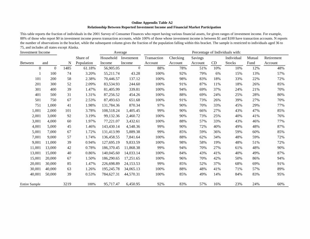
Investment Income

Between and N0 0 1485 61.18% 56,905.05 0 88% 78% 51% 10% 10% 12% 48%1 100 74 3.20% 55,211.74 43.28 100% 92% 79% 6% 15% 13% 57%

101 200 58 2.38% 70,446.57 137.12 100% 98% 83% 18% 33% 22% 72%201 300 52 2.09% 83,534.93 244.60 100% 91% 87% 11% 18% 26% 85%301 400 39 1.47% 81,405.99 339.81 100% 94% 69% 37% 24% 21% 70%401 500 31 1.31% 87,256.52 454.26 100% 88% 69% 24% 25% 28% 80%501 750 67 2.53% 87,493.63 651.68 100% 91% 73% 26% 39% 27% 70%751 1,000 41 1.98% 131,784.36 870.34 97% 90% 70% 33% 45% 29% 77%

1,001 2,000 101 3.78% 108,518.24 1,405.45 99% 90% 66% 27% 43% 47% 85%2,001 3,000 92 3.19% 99,132.36 2,460.72 100% 90% 73% 25% 40% 41% 76%3,001 4,000 60 1.97% 77,221.07 3,432.61 100% 88% 57% 33% 43% 46% 77%4,001 5,000 45 1.46% 143,430.14 4,548.36 99% 90% 72% 40% 49% 48% 87%5,001 7,000 67 1.72% 131,413.99 5,889.38 99% 85% 59% 36% 59% 60% 85%7,001 9,000 57 1.74% 136,458.55 7,841.64 100% 88% 62% 34% 48% 59% 72%9,001 11,000 39 0.94% 127,695.19 9,833.59 100% 98% 58% 19% 48% 51% 72%

11,001 13,000 42 0.78% 186,370.45 11,868.38 99% 94% 70% 27% 61% 48% 90%13,001 15,000 40 0.86% 140,045.60 14,033.14 100% 84% 43% 41% 40% 49% 87%15,001 20,000 67 1.50% 186,290.65 17,251.65 100% 96% 70% 42% 50% 86% 94%20,001 30,000 85 1.47% 226,698.89 24,153.53 99% 85% 52% 37% 68% 69% 91%30,001 40,000 63 1.26% 195,245.78 34,065.13 100% 88% 48% 41% 71% 57% 89%40,001 50,000 39 0.53% 784,627.31 44,570.31 100% 85% 49% 14% 84% 83% 95%

Entire Sample 3219 100% 95,717.47 6,450.95 92% 83% 57% 16% 23% 24% 60%

Online Appendix Table A2

Transaction Account

Checking Account

Savings Account CD

Individual Stocks

Mutual Fund

Retirement Account

This table reports the fraction of individuals in the 2001 Survey of Consumer Finances who report having various financial assets, for given ranges of investment income. For example, 88% of those who report $0 in investment income posess transaction accounts, while 100% of those whose investment income is between $1 and $100 have transaction accounts. N reports the number of observations in the bracket, while the subsequent column gives the fraction of the population falling within this bracket. The sample is restricted to individuals aged 36 to 75, and includes all states except Alaska.

Percentage of Individuals with:Share of Population

Household Income

Investment Income

Average

Relationship Between Reported Investment Income and Financial Market Participation

Panel A: Census Outcomes

Indicator: Income from Investments >

$500

Indicator: Income from Investment >

"Cutoff" (SCF)

Indicator: Income from Investment >

"Cutoff" (SIPP)

Amount of Income from Investments

Indicator: Income from Retirement

Savings

Amount of Income from Retirement

Savings

(1) (2) (3) (4) (5) (6) (7) (8)

Years of Schooling 0.069 *** 0.078 *** 0.093 *** 0.161 *** 0.105 *** 1756.75 *** 0.064 *** 1009.94 ***(0.005) (0.005) (0.007) (0.018) (0.016) (126.59) (0.010) (128.58)

Num of Observations 14,913,356 14,913,356 14,913,356 14,913,356 4,053,909 14,838,407 4,150,828 4,117,987F-stat of Excluded Instruments 37.7 48.5 48.5 48.5 7.96 48.4 45.8 45.3

Earned Income Spline No Yes Yes Yes Yes Yes Yes Yes

Panel B: SIPP Outcomes(1) (2) (3) (4) (5) (6)

Years of Schooling -0.002 0.003 0.0650 *** 0.0680 *** 0.040 * 0.044 **(0.031) (0.027) (0.022) (0.020) (0.024) (0.021)

Num of Observations 171,361 168,946 265,173 262,245 273,329 270,316 F-stat of Excluded Instruments 8.416 12.067 8.416 12.067 8.416 12.067

Earned Income Spline No Yes No Yes No Yes

Online Appendix Table A3

Indicator: Any Income from Investments

Indicator: Any Transactions Account

Indicator: Any Bond or Government Securities

Indicator: Any Stocks or Mutual Funds

IV Estimates of the Effect of Years of Schooling on Income from Various Sources with a 10-part Linear Spline in Earned Income

This table reports results from 2SLS regressions of income and assets on years of schooling, gender, race, age (3-year age groups), birth cohort (10 year cohorts), state of birth, state of residence, survey year and (where noted) a 10-part linear spline in earned income. Only the education coefficient is reported. The first stage is a regression of years of schooling on compulsory attendance dummies for grades 9, 10, and 11 or more (requiring 8 or fewer years is the omitted category). Regressions also include state of birth fixed effects interacted with a dummy variable for being born in the South and turning age 14 in 1958 or later to account for the impact of Brown v. Board of Education. We include 18-75 year olds (50-75 year olds when considering retirement income). In Panel A, the sample comprises individuals reported in the 5% samples of the 1980, 1990, and 2000 Censuses. The dependent variable of interest is whether the household receives income from investments or retirement savings and the amount. In Column 4, "Cutoff (SCF)" is predicted from an OLS regression of other interest income on age, race, sex, earned income, and year indicators, where the sample includes households from the 1983, 1992, and 2001 SCF with other interest income less than $50,000. In Column 5, "Cutoff (SIPP)" is predicted from an OLS regression of savings account interest on age, earned income, race, sex, and state of residence indicators, where the sample includes individuals from the 2001 SIPP. In Panel B, the sample comprises individuals from the 1990-2008 SIPP waves (Columns 1-2) and the 1984-2008 SIPP waves (Columns 3-6). In Panel A, Columns 6 and 8, top-coded individuals (see text) are dropped. Standard errors, corrected for arbitrary correlation within state of birth-year of birth, are in parentheses. (Numbers with *, **, or *** indicate significance at the 10-, 5-, or 1-percent level, respectively.)

Income source:

Panel A: All years, min of upper limit, max of lower limitYears of Schooling 2001.36 *** 1270.72 ***

(143.87) (172.82)

Num of Observations 14,913,356 4,150,828

Panel B: Data from 1990Education 2671.77 *** 1167.22 ***

(207.27) (183.15)

Num of Observations 5,235,729 2,000,968

Panel C: Data from 2000Years of Schooling 1943.03 ***

(274.27)

Num of Observations 4,053,909

(1) (2)

Online Appendix Table A4Tobit IV Estimates of the Effect of Schooling on Income from Various Sources

This table reports the second-stage relationship between investment income and educational attainment, using a Tobit model to deal with top- and bottom- coded dependent variables. The dependent variable of interest is the amount of income from investments the household receives. The sample comprises individuals reported in the 5% samples of the 1980, 1990, and 2000 census in Panel A, the data from 1990 in Panel B and 2000 in Panel C. (Unfortunately, regressions using only 1980 data and only 2000 data for Column 2 did not converge.) We include 18-75 year olds (50-75 year olds when considering retirement income). The independent variable of interest, years of schooling, is instrumented with compulsory schooling laws. In addition, we include as controls, but do not report, fixed effects for gender, race, 3-year age groups, 10-year birth cohorts, state of birth, state of residence, census year and a cubic polynomial in earned income. Regressions also include state of birth fixed effects interacted with a dummy variable for being born in the South and turning age 14 in 1958 or later to account for the impact of Brown v. Board of Education. Standard errors, corrected for arbitrary correlation within state of birth-year of birth, are in parentheses. (Numbers with *** indicate significance at the 1-percent level.)

Income from Investments

Income from Retirement Savings

Panel A: Census Outcomes

Indicator: Income from Investments >

$500

Indicator: Income from Investment >

"Cutoff" (SCF)

Indicator: Income from Investment >

"Cutoff" (SIPP)

Amount of Income from Investments

Indicator: Income from Retirement

Savings

Amount of Income from Retirement

Savings

(1) (2) (3) (4) (5) (6) (7) (8)

High School 0.33 *** 0.37 *** 0.44 *** 0.814 *** 0.588 *** 8893.41 *** 0.22 *** 5441.86 ***(0.03) (0.03) (0.04) (0.097) (0.101) (589.89) (0.06) (679.25)

Num of Observations 14,913,356 14,913,356 14,913,356 14,913,356 4,053,909 14,838,407 4,150,828 4,117,987F-stat of Excluded Instruments 47.6 52.4 52.4 52.4 12.27 52.1 66.6 66.6

Cubic Control for Income No Yes Yes Yes Yes Yes Yes Yes

Panel B: SIPP Outcomes(1) (2) (3) (4) (5) (6)

High School -0.052 -0.028 0.224 ** 0.267 *** 0.277 *** 0.317 ***(0.151) (0.143) (0.091) (0.093) (0.103) (0.100)

Num of Observations 171,361 168,946 265,173 262,245 273,329 270,316 F-stat of Excluded Instruments 18.60 20.80 18.597 20.8 18.60 20.80

Cubic Control for Income No Yes No Yes No Yes

Online Appendix Table A5

This table reports results from 2SLS regressions of income and assets on high school completion, gender, race, age (3-year age groups), birth cohort (10 year cohorts), state of birth, state of residence, survey year and (where noted) a cubic polynomial in earned income. Only the education coefficient is reported. The first stage is a regression of a high school completion dummy on compulsory attendance dummies for grades 9, 10, and 11 or more (requiring 8 or fewer years is the omitted category). Regressions also include state of birth fixed effects interacted with a dummy variable for being born in the South and turning age 14 in 1958 or later to account for the impact of Brown v. Board of Education. We include 18-75 year olds (50-75 year olds when considering retirement income). In Panel A, the sample comprises individuals reported in the 5% samples of the 1980, 1990, and 2000 Censuses. The dependent variable of interest is whether the household receives income from investments or retirement savings and the amount. In Column 4, "Cutoff (SCF)" is predicted from an OLS regression of other interest income on age, race, sex, earned income, and year indicators, where the sample includes households from the 1983, 1992, and 2001 SCF with other interest income less than $50,000. In Column 5, "Cutoff (SIPP)" is predicted from an OLS regression of savings account interest on age, earned income, race, sex, and state of residence indicators, where the sample includes individuals from the 2001 SIPP. In Panel B, the sample comprises individuals from the 1990-2008 SIPP waves (Columns 1-2) and the 1984-2008 SIPP waves (Columns 3-6). In Panel A, Columns 6 and 8, top-coded individuals (see text) are dropped. Standard errors, corrected for arbitrary correlation within state of birth-year of birth, are in parentheses. (Numbers with **, or *** indicate significance at the 5-, or 1-percent level, respectively.)

Indicator: Any Income from Investments

Indicator: Any Transactions Account

Indicator: Any Bond or Government Securities

Indicator: Any Stocks or Mutual Funds

IV Estimates of the Effect of High School Completion on Income from Various Sources

Years of Schooling -0.0021 * 0.011 -0.026 *** 0.010 *** 0.009 ***(0.0011) (0.013) (0.007) (0.003) (0.003)

Num of Observations 4,303,627 10,240,086 8,231,828 13,013,023 9,400,737F-stat of Excluded Instruments 31.4 52.2 45.7 48.4 5.1

Online Appendix Table A6IV Estimates of the Effect of Schooling on Possible Mechanisms from Various Sources

Dependent Variable:

The sample comprises individuals reported in the 5% samples of the 1980, 1990, and 2000 Censuses, except column (5) which only uses 1990 and 2000 data. The sample includes individuals who are aged 18-75 and born before 1965. The independent variable, years of schooling, is instrumented using compulsory schooling laws. Other controls include fixed effects for gender, race, 3-year age groups, 10-year birth cohorts, state of birth, state of residence, census year and a cubic polynomial in earned income. Regressions also include state of birth fixed effects interacted with a dummy variable for being born in the South and turning age 14 in 1958 or later to account for the impact of Brown v. Board of Education. In Column 1, the dependent variable is whether or not an individual reports negative investment income, conditional on having any non-zero investment income. In Columns 2 and 3, the dependent variable is whether the individual has a first or second mortgage, respectively. In Column 4, the dependent variable is the share of individuals aged 65-70 in 1970 in the same occupation and state who report receiving retirement income. In Column 5, the dependent variable is the share of neighbors in the current year aged 65 and above who report receiving retirement income other than Social Security. (Numbers with *, or *** indicate significance at the 10-, or 1-percent level, respectively.)

Reports Negative Investment Income

Share of Employees in Occupation with

Pension

Share of Neighbors with Pension

(4) (5)(1)

Has a First Mortgage

Has a Second Mortgage

(2) (3)

Variable Year(s) Mean St. Dev. Min Max(1) (2) (3) (4) (5)

Knowledge 1981 58.71 22.47 0 119Ability 1981 117.82 40.74 0 213Cognitive Ability 1981 36.81 28.19 1 99Years of Education 1985 - 2004 12.94 2.33 0 20Age (in year 1979) 1979 17.16 2.06 14 22Male 1979 0.52 0.50 0 1Total Net Family Income 1979 - 2004 51197.32 85407.59 0 1637987Pearlin "Little Control Over Life" 1992 1.80 0.67 1 4

Any …Money Left 1990 - 2004 0.66 0.48 0 1Savings 1985 - 2000 0.64 0.48 0 1Stocks, Bonds & Mutual Funds 1988 - 2000 0.16 0.37 0 1IRAs & Keogh 1994 - 2000 0.19 0.40 0 1Tax-Deferred Accounts 1994 - 2000 0.33 0.47 0 1CDs, Loans, Mortgage Assets 1994 - 2000 0.05 0.22 0 1Rights to Estate, Investment Trust 1988 - 2000 0.03 0.18 0 1Income from Other Sources 1979 - 2002 0.30 0.46 0 1

Amount …Money Left 1990 - 2004 65147 103348 1 989100Savings 1985 - 2000 6699 24144 0 835000Stocks, Bonds & Mutual Funds 1988 - 2000 2556 19379 0 989100IRAs & Keogh 1994 - 2000 4671 23928 0 549500Tax-Deferred Accounts 1994 - 2000 9513 33984 0 549500CDs, Loans, Mortgage Assets 1994 - 2000 1014 11397 0 549500Rights to Estate, Investment Trust 1988 - 2000 2236 40288 0 3114800Income from Other Sources 1979 - 2002 500 3373 0 168780

Online Appendix Table A7Summary Statistics, NLSY

Summary statistics are from the National Longitudinal Survey of Youth. The survey was conducted annually from 1979-1984, and biennially since 1996. Column (1) indicates the years from which data are used.

Dependent Variable:

Years

Panel A: Any $ in AssetKnowledge 0.034 *** 0.011 0.012 0.005 -0.0001 -0.006 0.053 ***

(0.011) (0.009) (0.015) (0.017) (0.008) (0.004) (0.009)Ability 0.018 * 0.052 *** 0.019 0.053 *** 0.012 * 0.001 0.041 ***

(0.009) (0.009) (0.014) (0.015) (0.007) (0.004) (0.008)Years of Schooling 0.015 *** 0.017 *** 0.011 ** 0.013 ** 0.003 -0.001 0.015 ***

(0.003) (0.003) (0.005) (0.005) (0.002) (0.001) (0.002)

Num of Observations 34663 44006 14220 14195 14239 34696 76372R-Squared 0.33 0.42 0.42 0.39 0.24 0.22 0.39p-value of F test of Knowledge 0.00 0.00 0.07 0.00 0.10 0.28 0.00 & AbilityPanel B: AmountKnowledge 675.00 128.79 738.06 1941.61 -590.42 -325.91 30.47

(607.50) (661.15) (835.20) (1304.07) (438.99) (1004.00) (56.96)Ability 341.56 1062.63 * -457.82 1252.57 581.09 -464.20 -18.71

(473.45) (564.66) (751.55) (1217.84) (449.59) (780.39) (45.02)Years of Schooling 314.67 * 299.39 * 597.71 ** 628.54 35.83 -82.46 90.19 ***

(183.34) (181.33) (299.90) (448.31) (128.89) (269.70) (17.97)

Num of Observations 33455 44432 13645 13174 14103 34118 74277R-Squared 0.19 0.26 0.34 0.38 0.16 0.12 0.11p-value of F test of Knowledge 0.06 0.02 0.68 0.01 0.36 0.58 0.86 & Ability

(7)1985 - 2000 1988 - 2000

Rights to Estate, Investment

Trust

Tax-Deferred Accounts

1994 - 2000 1994 - 20001994 - 2000(4) (5)

1988 - 2000(6)

1988 - 2000(1) (2) (3)

Online Appendix Table A8

Income from Other Sources (Interest,

Rent, Dividends, etc.)

IRAs & Keogh

Estimates of the Effect of Knowledge and Ability on Savings, NLSYData are from the National Longitudinal Survey of Youth. Panel A reports whether the individual has any money in any of the listed assets, and Panel B gives the amount in dollars. Cognitive ability (knowledge and ability) is measured by tests given around age 17. Additional controls included are sibling-group fixed effects, family income in every year with dummies proxying for missing data and fixed effects for age, gender, race, survey year, birth order and birth year. Standard errors are clustered at the individual level. (Numbers with *, **, or *** indicate significance at the 10-, 5-, or 1-percent level, respectively.)

SavingsCDs, Loans,

Mortgage Assets

Stocks, Bonds & Mutual

Funds

Dependent Variable:

Panel A: Any Money Little Control 0.01 -2.09 ** -1.20 -1.54 -0.26 0.10 -1.44 *

(0.79) (0.89) (0.92) (1.08) (0.48) (0.34) (0.77)

Num of Observations 21,261 17,593 13,831 13,807 13,851 21,292 24,503 R-Squared 0.38 0.49 0.42 0.40 0.24 0.26 0.45

Panel B: AmountLittle Control 27.73 186.16 -221.19 -1276.97 3.88 -85.34 -14.40

(527.41) (612.54) (510.84) (835.30) (198.17) (743.49) (67.58)

Num of Observations 20,399 18,720 13,277 12,823 13,721 20,924 23,558 R-Squared 0.24 0.37 0.35 0.38 0.16 0.17 0.21

IRAs & Keogh

CDs, Loans, Mortgage

Assets

(5)

Online Appendix Table A9

Data are from the National Longitudinal Survey of Youth. Panel A reports whether the individual has any money in any of the listed assets, and Panel B gives the amount in dollars. The independent variable of interest is a measure of whether the respondent agrees with the statement “I have little control over the things that happen to me,” with 1 indicating strong disagreement and 4 indicating strong agreement. Additional controls included are sibling-group fixed-effects, family income in every year with dummies proxying for missing data and fixed effects for age, gender, survey year, birth order and birth year. Standard errors are clustered at the individual level. (Numbers with *, **, or *** indicate significance at the 10-, 5-, or 1-percent level, respectively.)

(3) (4) (6)

Stocks, Bonds & Mutual Funds

(1)

Tax-Deferred Accounts

Rights to Estate,

Investment Trust

Estimates of the Effect of Not Feeling in Control on Savings, NLSY

Income from Other Sources (Interest, Rent, Dividends,

etc.)

(7)(2)

Savings