sme policies as a barrier to growth of smes · 1 rieti discussion paper series 17-e-046 march 2017...
TRANSCRIPT

DPRIETI Discussion Paper Series 17-E-046
SME Policies as a Barrier to Growth of SMEs
TSURUTA DaisukeNihon University
The Research Institute of Economy, Trade and Industryhttp://www.rieti.go.jp/en/
1
RIETI Discussion Paper Series 17-E-046
March 2017
SME Policies as a Barrier to Growth of SMEs†
TSURUTA Daisuke
College of Economics, Nihon University
Abstract We investigate whether firms have incentives to retain their positions as small and medium enterprises (SMEs)
to benefit from various SME policies. Using small business data from Japan, we show that firms are less likely
to increase their registered capital so that they can continue to satisfy the requirement that retains their position
as SMEs under the SME Basic Act. In addition, we find that, after the relaxation of this SME requirement under
the act, firms were more likely to increase their registered capital. When firms do not increase their registered
capital in order to keep their SME status, firm growth is impeded.
Keywords: SME policy, Firm growth, Equity capital, Small businesses
JEL classification: L53; L25; G32
RIETI Discussion Papers Series aims at widely disseminating research results in the form of professional
papers, thereby stimulating lively discussion. The views expressed in the papers are solely those of the
author(s), and neither represent those of the organization to which the author(s) belong(s) nor the Research
Institute of Economy, Trade and Industry.
† This study was conducted as part of the “Study on Corporate Finance and Firm Dynamics” project at the Research Institute of Economy, Trade, and Industry (RIETI). This study uses microdata from the Surveys for the Financial Statements Statistics of Corporations by Industry (Houjin Kigyou Toukei Chosa) conducted by the Ministry of Finance. This study was supported by a Grant-in-Aid for Scientific Research (C) #16K03753 from the Japan Society for the Promotion of Science. The author would also like to thank Fumio Akiyoshi, Hikaru Fukanuma, Kaoru Hosono, Daisuke Miyakawa, Masayuki Morikawa, Yoshiaki Ogura, Hiroshi Ohashi, Arito Ono, Kuniyoshi Saito, Daisuke Shimizu, Hirofumi Uchida, Iichiro Uesugi, WakoWatanabe, Peng Xu, and Makoto Yano for many valuable comments. The seminar participants at RIETI also provided useful comments. All remaining errors are mine.

1 Introduction
We investigate whether policies for small and medium enterprises (SMEs) impede incen-
tives to graduate from SME status. Economic theories justify the use of SME policies
when market failure occurs (Storey, 1994). First, owing to the information gap between
lenders and borrowers, credit rationing is serious for SMEs (Berger and Udell, 1998). To
enhance credit supply for SMEs, the government establishes public lending and credit
guarantee schemes, which can improve social welfare (Mankiw, 1986). Therefore, public
financial supports for SMEs can be justified from the point of view of economic theory.1
Second, if the spillover of knowledge from R&D investment is significant,2 the benefits
from innovation spread to other firms that do not pay the cost of investment. If the
positive externality relating to spillovers from innovation is significant, underinvestment
for R&D might be serious, which causes market failure.
As Storey (1994) argues, the aim of actual SME policies is ambiguous from an economic
viewpoint. Many SME policies exist even if market failure does not occur, and an excessive
menu of SME policies is adopted in many countries. One of the reasons for the excessive
use of SME policies is that many government departments feel that SMEs should be
supported by economic policies and regard SMEs as “their responsibility” (Storey, 2008).
As a result, Storey (2008) shows that, in the UK, SME policies give rise to expenditure
of around 8 billion euro, which is approximately the same spending required to maintain
a police force.
According to the Small and Medium Enterprise Agency in Japan, the initial general
account budget for SME policies in Japan was 180.2 billion yen,3 and the supplementary
budget was 543.4 billion yen in fiscal year (FY) 2012.4 According to Goto (2014), the
1Because of government failure, public financial support does not always improve social welfare.2Acs and Szerb (2007), for instance, argue that this is the case.3This excludes the budget for the Great East Japan Earthquake.4See Chusho Kigyou Shisaku Souran (Overview of SME Policy) for more detailed in-
formation, downloadable from the website of the Small and Medium Enterprise Agency(http://www.chusho.meti.go.jp/pamflet/souran/2013/).
2

budget for SME policies was 2.9% of the total budget in FY2009, which was not particu-
larly large.5 On the other hand, as shown in Table 1, which provides a list of SME policies
compiled by the Ministry of Economy, Trade and Industry (METI) in Japan, the menu
of SME policies is large. In addition to these policies, the Ministry of Finance (MOF)
reduces corporate tax for firms that satisfy SME requirements.
Often, the government implements SME policies even when market failure is not se-
rious. For example, Table 1 describes that the policy program of business innovation
“assists SMEs undergoing business innovation in financing, handling taxes and cultivat-
ing markets.” The aim of this program is not to support innovation that has spillovers
to other firms and, thus, the program does not mitigate the market failure caused by this
positive externality. Instead, the program simply aims to enhance the efficiency of the
management of SMEs, which is not an intervention that is justified by market failure.
Furthermore, SMEs can participate in various policy programs that assist in enhancing
management of SMEs. For example, Table 1 shows that the program “Trade practices
and public procurement” increases the opportunity for SMEs to win contracts in govern-
ment offices. Because SMEs cannot always supply a higher quality of goods or services
compared with large firms, SME policy should not increase their opportunities to win con-
tracts because this reduces market efficiency. As noted above, corporate tax is reduced
for all SMEs, which is another policy that is not justified by market failure.
Although a public credit guarantee is justified by severe market failure, the amount of
credit guarantee provided is often excessive. OECD (2016) points out that “SMEs receive
substantial government support, particularly through a large credit guarantee system,
which supports about 40% of Japanese SMEs” (p. 16).6 The substantial government
financial support can enhance growth of SMEs by relaxing credit constraints. OECD
(2016) also notes that this policy “has contributed to a delayed restructuring in the
5Goto (2014) also points out that if the amount of reduced corporate tax is included, the budget forSME policies is much larger.
6According to OECD (2013), the volume of credit guarantees as a percentage of GDP is 7.3% in Japan,the highest among the listed countries.
3

business sector, created some disincentives to grow and hindered the development of
market-based financing” (p. 16).
In sum, SMEs receive substantial government support through a wide variety of SME
policies and, as OECD (2016) argues, these policies reduce incentives for growth by SMEs.7
Firms cannot benefit from the huge range of SME policies listed in Table 1 if they outgrow
their SME status and become large firms.8 In addition, if a firm graduates from an
SME to a large firm, it cannot access the public credit guarantee. During periods of
financial crisis (in particular, the global financial crisis in 2008), additional public credit
guarantee programs commenced, which enabled SMEs to access guaranteed loans more
easily, thereby enhancing their liquidity. Furthermore, firms are required to pay higher
corporate tax if they graduate from SME status. Because they wish to retain their access
to the various SME policies available, firms do not have the incentive to graduate from
SME status, which impedes firm growth.
Many previous studies empirically investigate the effects of several SME policies. Nu-
merous studies (for example, Kang and Heshmati, 2008; Oh et al., 2009; Craig et al.,
2007) show empirically that the public credit guarantee program has positive effects on
employment, sales, and local growth, and that it reduces the default and bankruptcy
rates of SMEs. In Japan, Uesugi et al. (2010) find that special credit guarantee pro-
grams improved the availability of credit for SMEs during the financial crisis. In contrast,
Ono et al. (2013) find that although the program eased credit availability, the ex post
performance of SMEs that received a credit guarantee deteriorated compared with other
firms. Honjo and Harada (2006) show that the SME Creative Business Promotion Law
enacted by the Government of Japan provides support to SMEs to enter new areas of
7OECD (2016) notes that “small companies in Japan tend to remain small, in part because high publicsupport discourages small firms from growing because they would lose the benefits associated with SMEstatus” (p. 11).
8For example, the policies result in SMEs winning contracts even if their production ability andefficiency are not as high as larger firms, so the policies enhance the profitability of SMEs. In otherwords, if firms grow from SMEs into large firms, they cannot participate in these policy programs andthis reduces their opportunities to win contracts.
4
business and enhances firm growth for SMEs. Although a number of reports focus on the
effects of individual SME policies, few studies have investigated whether the substantial
government support for SMEs has a negative effect on firm growth.
In this paper, we investigate whether the various SME policy programs in Japan
impede the growth of firms from SMEs to large firms. To test this question, we employ
two strategies. First, we focus on the definitions of SMEs under the Corporation Tax
Act, which defines SMEs as firms with registered capital of 100 million yen or less. We
investigate whether SMEs that are close to this cap for registered capital (i.e., 100 million
yen) are less likely than other firms to increase their registered capital so that they can
remain within the definitions of SMEs and retain their access to the SME policy programs.
Second, for our analysis, we use the changes in the Small and Medium-sized Enterprise
Basic Act (the SME Basic Act) in Japan that came into effect in December 1999. In Japan,
only firms that satisfy the definitions of SMEs under the SME Basic Act can participate
in the SME policy programs listed in Table 1. Before 1999, SMEs were defined as firms
with 100 or fewer regular employees or with 100 million yen of registered capital or less
(except for firms in the wholesale, retail, and service industries). Following revision of
the SME Basic Act, the requirement for registered capital was changed to 300 million yen
or less, so that firms could increase registered capital but still satisfy the requirements
of the SME Basic Act. As Table 2 shows, the definitions of SMEs differ for firms in the
wholesale, retail, and service industries.
By focusing on the change of the SME Basic Act as an exogenous event, we can test
whether firms have incentives to retain their SME status even if they can graduate to large
firms. If firms do not graduate from SME status, but could have done so if they wished,
this is indicated by the firms then increasing their registered capital after the change
of the SME Basic Act, which relaxed the registered capital requirement. Furthermore,
by focusing on the difference in the requirement for SMEs between industries, we can
test the hypothesis using the difference-in-differences approach. As Table 2 shows, the
5
registered capital requirement changed from 100 million yen to 300 million yen for a firm
in a manufacturing industry with the change in the SME Basic Act. On the other hand,
in the wholesale, retail, and service industries, firms were required to have registered
capital of 100 million yen or less both before and after the change in the SME Basic
Act. Therefore, we can use the subsample of firms in the wholesale, retail, and services
industries as a control group and those in the other industries as a treatment group.
Similarly, by focusing on the change in the registered capital requirement for wholesale,
retail, and service industries, we can use firms in those industries as a treatment group,
and those in other industries as a control group.
The main findings of this paper are as follows. First, firms with registered capital of
100 million yen or less (i.e., SMEs under the definitions in the Corporation Tax Act and
the SME Basic Act before it was altered in 1999) are less likely to increase registered
capital, compared with firms with registered capital of over 100 million yen. This implies
that SMEs have a disincentive to increase their registered capital because they benefit
from keeping their SME status. Second, after the change in the definition of SMEs under
the SME Basic Act in 1999, which involved the increase in the registered capital limit,
firms that satisfied the previous SME requirement (registered capital of 100 million yen
or less) then increased their registered capital. This effect is larger if a firm’s registered
capital is close to the registered capital requirement under the original SME Basic Act
and the Corporation Tax Act. These effects are robust because they are supported if we
estimate them using a different treatment group. Third, firms that increase registered
capital increase firm size (in terms of asset growth). As firms have a disincentive to
increase registered capital so that they can keep their SME status, this indicates that the
SME requirements are significant constraints on firm growth. Additionally, firms decrease
debts by increasing equity if they are highly leveraged or highly volatile. This implies
that firms are able to adjust to an optimal capital structure after the relaxation of their
registered capital requirements.
6
Our study is related to studies that use the calibrations of a theoretical model to argue
that policies that depend on firm size cause distortions of firm size. For example, Garicano
et al. (2016) and Gourio and Roys (2014) focus on the many labor laws in France that
are binding for firms with 50 employees or more and estimate the welfare costs of these
regulations. Guner et al. (2006) and Guner et al. (2008) show, using the Lucas model,
that size-dependent laws, such as Japan’s Large Scale Retail Location Law, distort the
firm-size distributions. Garcıa-Santana and Pijoan-Mas (2014) focus on the Small Scale
Reservation Laws in India that reserve several products for production by small-scale
industries. They also use the Lucas model to show that this policy decreases the output
per worker by 2% in the whole economy.
Similarly to these previous studies, our study finds that size-dependent policies impede
firm growth by small businesses. However, this paper differs from the existing literature
in three ways. First, whereas the previous studies employ simulations from theoretical
models, we employ a difference-in-differences approach using the change in the SME
Basic Act as an exogenous event and we utilize not a macroeconomic model but an
econometric model, using firm-level data of small businesses. Second, we differ from the
studies focusing on France because, in contrast to the labor laws in France, the SME
policy that we study in Japan aims to promote the development of small businesses.9 We
show that the SME policy impedes firm growth of small businesses through decreases in
equity capital, which is contrary to its aim. Third, we focus not only on firm growth, but
also on the financial activities of small businesses.
The remainder of the paper is organized as follows. Section 2 provides the definitions
of SMEs under the Corporation Tax Act and the SME Basic Act. Section 3 describes
the data set. Section 4 introduces the empirical strategy and hypotheses for the relation-
ships between SME policies, registered capital, and firm growth. Section 5 provides the
estimation results for the hypotheses. Section 6 concludes the paper.
9see http://www.chusho.meti.go.jp/soshiki/ninmu.html regarding the aim of the Small and MediumEnterprise Agency in Japan.
7

2 Definitions of SMEs in Japan
2.1 Corporation Tax Act
There are several definitions of SMEs in Japan, with the major definitions being those
of the SME Basic Act and the Corporation Tax Act. Under the Corporation Tax Act,
SMEs are defined as firms with 100 million yen of registered capital or less (Panel A of
Table 2). Corporate tax is reduced for firms that satisfy the definition of an SME under
the Corporation Tax Act. For example, the corporate tax rate for SMEs is 22%, which is
applied to incomes under 8 million yen. The corporate tax rate for large firms between
1999 and 2012 was 30%.10 Therefore, if firms satisfy the definition of SMEs under the
Corporation Tax Act, they can pay a low corporate tax and increase their cash flow.
2.2 SME Basic Act
As shown in Panel B of Table 2, the definition of SMEs in the SME Basic Act is not
simple. The definitions of SMEs before December 1999 are as follows.
• SMEs under the SME Basic Act are defined as firms with 100 million yen of regis-
tered capital or less and/or 300 or fewer regular employees.
• SMEs in the wholesale industry are defined as firms with 30 million yen of registered
capital or less and/or 100 or fewer regular employees.
• SMEs in the retail industry and the service industry are defined as firms with 10
million yen of registered capital or less and/or 50 or fewer regular employees.
In December 1999, the SME Basic Act was revised and the registered capital require-
ment was relaxed. The revised requirement for SME status after December 1999 is as
follows.
10See the website of the Ministry of Finance in Japan (http://www.mof.go.jp/tax policy/summary/corporation/082.htm(in Japanese, last date accessed: September 2016)) regarding the corporate tax rate trends.
8
• SMEs under the SME Basic Act are defined as firms with 300 million yen of regis-
tered capital or less and/or 300 or fewer regular employees.
• SMEs in the wholesale industry are defined as firms with 100 million yen of registered
capital or less and/or 100 or fewer regular employees.
• SMEs in the retail industry are defined as firms with 50 million yen of registered
capital or less and/or 50 or fewer regular employees.
• SMEs in the service industry are defined as firms with 100 million yen of registered
capital or less and/or 100 or fewer regular employees.
3 Data
We use annual firm-level data from the Surveys for the Financial Statements Statistics
of Corporations by Industry (hereafter FSSC; Houjin Kigyou Toukei Chosa in Japanese),
conducted by the Ministry of Finance. According to the website of the Ministry of Fi-
nance,11 the FSSC are “one part of the fundamental statistical surveys under the Statistics
Act and have been conducted as sampling surveys so as to ascertain the current status of
business activities of commercial corporations in Japan.” The target firms of the FSSC
are all commercial corporations in Japan. All firms with capital of one billion yen or
more are included. Those with capital of between 100 million and 600 million yen are
randomly selected with equal probability. Those with less than 100 million yen of capital
are randomly sampled every fiscal year. Therefore, of the firms with less than 100 million
yen in capital, a different sample of target firms is selected each fiscal year. The response
rates for each fiscal year are around 80%. The FSSC include data on firms’ balance sheets
and profit and loss statements. Data on firms’ balance sheets are available at the be-
ginning and end of each fiscal year. The data at the end of fiscal year t are set equal
11For details of the survey see: http://www.mof.go.jp/english/pri/reference/ssc/index.htm (last dateaccessed: June 2016).
9

to the data at the beginning of fiscal year t + 1. We use observations from FY1991 to
FY2007. To exclude large firms, the sample is limited to firms with 500 million yen or
less of registered capital. We choose the sample period FY1991–FY2007 to exclude the
effects of the bubble economy before 1990 and the global financial crisis after 2008. The
number of full firm-year observations is 306,353 during the period FY1991–FY2007.
4 Empirical Strategy
4.1 Effects of the Cap on Registered Capital
4.1.1 Hypothesis
As described in the previous section, the cap on registered capital in the definition of
SMEs under the Corporation Tax Act is 100 million yen. If firms have an incentive to
retain their SME status and observe the SME requirements to save corporate tax, they
will not increase their registered capital over 100 million yen. We predict that firms with
registered capital close to 100 million yen are less likely to increase their registered capital.
In addition, under the SME Basic Act, the caps on registered capital in the definitions
of SMEs are 10, 30, 100, or 300 million yen, depending on the industry and the year.
We predict that firms with registered capital close to these caps are less likely to increase
their registered equity.
4.1.2 Equation
To test our hypothesis, we estimate the following equation:
∆R Capitali,t =∑
αj1R Capital Dummyj
i,t + Xi,tα2 + ζt + ηi + θi,t (1)
10

where θi,t is the error term of firm i in fiscal year t, ηi is industry fixed effects of 45
industries, and ζi is year fixed effects from FY1991 to FY2007. We use two definitions of
∆R Capitali,t. One is a dummy variable that has a value of one if registered capital at the
end of fiscal year t is larger than at the beginning of fiscal year t (Additional R Capital
Dummy, shown as “Dummy” in tables). The other is the difference in registered capital
at the end of fiscal year t compared with that at the beginning of fiscal year t (Amount of
Additional R capital, shown as “Amount” in tables). X includes leverage at the beginning
of fiscal year t, tangible fixed assets at the beginning of fiscal year t, and operating incomes
in fiscal year t.
We focus on the effects of 18 types of R Capital Dummy. The definitions of each
dummy variable are shown in Table 3. If firms have an incentive to satisfy the requirements
under the Corporation Tax Act and the SME Basic Act, firms with registered capital close
to 100 million yen are less likely to increase their registered capital. Therefore, we predict
that the coefficient of R capital 100M is negative. In addition, compared with the effects
of the R capital 110M dummy and a similar level of registered capital dummies, the
magnitude of the negative effects is larger. Similarly, the caps of 30 and 300 million yen
under the SME Basic Act have significant effects on additional registered capital, and the
coefficients of R capital 30M and R capital 300M are negative.
According to Ou and Haynes (2006), funds for acquiring additional equity capital in
SMEs are determined by firm age, size, sales growth, financial condition, internal finan-
cial sources (such as owner loans or personal and business credit cards), and loans with
traditional or nontraditional institutions. We use leverage, cash holdings, tangible fixed
assets, operating incomes, firm size, and year and industry dummies as control variables.
Leverage is a proxy for financial condition and loans with traditional or nontraditional
institutions. Highly leveraged firms have easier access to loans from traditional or non-
traditional institutions. On the other hand, very highly leveraged firms are financially
distressed firms (as argued by Opler and Titman, 1994), so leverage is also a proxy for
11

financial condition. Because highly leveraged firms have incentives to increase equity
capital to mitigate their financial distress, we predict that leverage has positive effects
on additional equity capital. Leverage is defined as the book value of debt divided by
the book value of assets at the beginning of fiscal year t. Cash holdings are a proxy
for liquidity. We predict that firms with higher liquidity are less risky, so the effects on
additional registered equity are positive. Cash holdings are defined as cash holdings at
the beginning of fiscal year t, normalized by total assets at the beginning of fiscal year t.
Operating incomes are a proxy for financial condition. High operating incomes suggest
that firms have sufficiently high cash flows, which leads to low credit constraints. In
addition, operating incomes are a proxy for firm profitability. If firms with low cash flows
face credit constraints on bank loans and use additional equity capital, then the coefficient
of operating incomes will be negative. On the other hand, if profitable firms can use
additional equity, the coefficient of operating incomes will be positive. Operating income
is defined as operating income in fiscal year t, normalized by total assets at the beginning
of fiscal year t. Tangible fixed assets are variables representing the amount of collateral
assets. Firms with high collateral assets are less risky and have easier access to loans.
Therefore, tangible fixed assets are a proxy of financial condition and the availability of
loans with traditional or nontraditional institutions. Therefore, the coefficient of tangible
fixed assets is negative for additional equity capital if equity capital and bank loans are
substitutes. Tangible fixed assets are defined as tangible fixed assets at the beginning
of fiscal year t, normalized by total assets at the beginning of fiscal year t. Firm size is
controlled by the natural logarithm of total assets at the beginning of fiscal year t. Larger
firms are less risky and can use more capital. Therefore, we predict that the coefficient of
firm size is positive.
12

4.2 Effects of Changes in Requirements in the SME Basic Act
4.2.1 Hypothesis
In Japan, SMEs can access the various SME policies listed in Table 1. We predict that
firms ensure that they remain within the SME requirements under the SME Basic Act so
that they can utilize these SME policies, which is a disincentive for firm growth. If a firm’s
registered capital is close to the cap specified in the SME Basic Act, they do not have an
incentive to increase their registered capital. As a result, firms do not increase their equity
capital. To investigate this research question, we focus on the effects of the change in 1999
in the definition of SMEs in the SME Basic Act. As noted above, this change resulted in
the registered capital cap requirement being relaxed from 100 million to 300 million yen
for all industries, with the exception of wholesale, retail, and service industries. Following
the 1999 revision, firms with registered capital of around 100 million were able to increase
their equity capital but retain their SME status under the requirements of the new Act. If
the cap acts as an effective constraint on increases in registered capital, then firms would
increase their registered capital after the change in the SME Basic Act. These effects
would be magnified if a firm’s registered capital was close to the pre-1999 cap. As the cap
of 100 million yen does not apply to wholesale, retail, and service industries, we can regard
the firms in these industries as a control group. We employ the difference-in-differences
approach and test whether treatment group firms increased their registered capital after
the revision of the SME Basic Act.
Similarly, we test our hypothesis using the wholesale, retail, and service industries as
a treatment group and other industries as a control group. As noted above, the registered
capital cap rose from 30 million to 100 million for the wholesale industry with the changes
to the SME Basic Act. If the cap is an effective constraint, firms with a registered capital
of close to 30 million yen in the wholesale industry would not increase their registered
capital before the revision of the SME Basic Act. Also, this effect is significant for the
treatment group, that is firms in the wholesale industry in this case. The effect of the
13
gap between a firm’s registered capital and the cap of 30 million yen before the revision
is weaker after the revision of the SME Basic Act in the treatment group. Finally, we
investigate the case of the retail and service industries. In this case, the cap was 10 million
yen before the revision of the SME Basic Act, and so we focus on the gap between a firm’s
registered capital and the cap of 10 million yen.
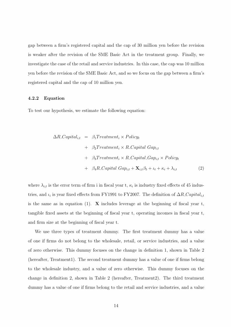
4.2.2 Equation
To test our hypothesis, we estimate the following equation:
∆R Capitali,t = β1Treatmenti × Policyt
+ β2Treatmenti × R Capital Gapi,t
+ β3Treatmenti × R Capital Gapi,t × Policyt
+ β4R Capital Gapi,t + Xi,tβ5 + ιt + κi + λi,t (2)
where λi,t is the error term of firm i in fiscal year t, κi is industry fixed effects of 45 indus-
tries, and ιi is year fixed effects from FY1991 to FY2007. The definition of ∆R Capitali,t
is the same as in equation (1). X includes leverage at the beginning of fiscal year t,
tangible fixed assets at the beginning of fiscal year t, operating incomes in fiscal year t,
and firm size at the beginning of fiscal year t.
We use three types of treatment dummy. The first treatment dummy has a value
of one if firms do not belong to the wholesale, retail, or service industries, and a value
of zero otherwise. This dummy focuses on the change in definition 1, shown in Table 2
(hereafter, Treatment1). The second treatment dummy has a value of one if firms belong
to the wholesale industry, and a value of zero otherwise. This dummy focuses on the
change in definition 2, shown in Table 2 (hereafter, Treatment2). The third treatment
dummy has a value of one if firms belong to the retail and service industries, and a value
14

of zero otherwise. This dummy focuses on the changes in definitions 3 and 4, shown in
Table 2 (hereafter, Treatment3).
In addition, we add variables indicating the registered capital gap (R Capital Gap in
Equation 2), which is defined as the natural logarithm of the cap on registered capital in
the SME Basic Act before 1999 minus a firm’s registered capital at the beginning of fiscal
year t. We define three types of registered capital gap, depending on the cap on registered
capital. R Capital Gap1 is defined as the natural logarithm of 100 million yen minus a
firm’s registered capital at the beginning of fiscal year t. R Capital Gap2 is defined as the
natural logarithm of 30 million yen minus a firm’s registered capital at the beginning of
fiscal year t. R Capital Gap3 is defined as the natural logarithm of 10 million yen minus
a firm’s registered capital at the beginning of fiscal year t. If firms do not increase their
registered capital so that they can continue to satisfy the SME requirements, the treated
firms with a smaller registered capital gap increase their lower registered capital.
If treated firms increase their registered capital after the change in the definitions of
SMEs in 1999, the coefficient of Treatmenti × Policyt is positive. Because treated firms
with registered capital close to the cap under the definition of SMEs have less incen-
tive to increase their registered capital, we predict that the coefficient of Treatmenti ×
R Capital Gapi,t is negative. In addition, if the incentive to increase registered capital
is weakened by the cap set in the definition of SMEs, firms will increase their registered
capital after the revision of the Act relaxed the cap. Therefore, because the effects of
Treatmenti ×R Capital Gapi,t are smaller after the change in the definition of SMEs, we
predict that the coefficient of Treatmenti × R Capital Gapi,t × Policyt is negative. The
coefficient of R Capital Gapi,t controls the effects of R Capital Gapi,t on ∆R Capitali,t
for both treated and control groups. We control the effects of Treatmenti by industry
fixed effects and those of Policyt by year fixed effects.
15

4.3 Consequences of Changes in Registered Capital
4.3.1 Hypothesis
As a consequence of increasing registered capital and acquiring additional equity capital,
firms can increase their inventory and/or capital investment, which induces asset growth
of firms. As these actions enhance firm value, we predict that the change in the SME
registered capital requirements will lead to firm growth.12 If this prediction is supported,
low levels of registered capital, caused by the cap in the definition of SMEs, impede firm
growth by decreasing acquisitions of equity capital. On the other hand, firms can use
other financial sources to finance investment opportunities, such as bank loans. In this
case, the effects of additional registered capital on firm growth are not significant.
In addition, we investigate the effects of equity issues on debt finance. If registered
capital constraints are severe for small businesses, they will use other financial sources,
including bank loans. As a result, we consider that, prior to the changes in the SME
Basic Act, firms would have used debt rather than equity beyond the level that was
optimal. If this is accurate, the coefficient of additional equity on total debt growth will
be negative. On the other hand, if the relationship between equity issues and debt finance
is complementary, the coefficient of additional equity will be positive. The reason for this
positive relationship is that firms with equity issues would become more creditworthy,
and the supply of bank loans would increase.
4.3.2 Equation
To investigate the consequence of additional equity capital, we estimate the following
regression:
Growthi,t = γ1∆R Capitali,t + Yi,tγ2 + µt + νi + ξi,t (3)
12The consequence of additional equity capital is not only firm growth. Ou and Haynes (2006) arguethat firms avoid defaulting on loans as additional equity capital mitigates liquidity shortages.
16

∆R Capital∗i,t = Zi,tω1 + Xi,tω2 + øt + πi + τi,t (4)
∆R Capitali,t = 1 if ∆R Capital∗i,t > 0
∆R Capitali,t = 0 otherwise
where xii,t ∼ N(0, σ2), τi,t ∼ N(0, σ2), and Cov(ξi,t, τi,t) = ρ = 0. νi and πi are industry
fixed effects of 48 industries and µt and øt are year fixed effects from FY1991 to FY2007.
We use two proxies of growth, asset growth and debt growth. Asset growth is defined
as the annual change in total assets from the beginning to the end of fiscal year t, which
is normalized by total assets at the beginning of fiscal year t. Debt growth is defined as
the annual change in total debts from the beginning to the end of fiscal year t, which
is normalized by total assets at the beginning of fiscal year t. We use the additional
registered capital dummy as a proxy of ∆R Capitali,t. Yi,t includes cash holdings at
the beginning of fiscal year t, leverage at the beginning of fiscal year t, tangible fixed
assets at the beginning of fiscal year t, operating income in fiscal year t, and firm size
at the beginning of fiscal year t. As we argued above, ∆R Capitali,t is determined by
many variables, which include the level of a firm’s registered capital and the change in
the definition of SMEs. Therefore, because ∆R Capitali,t is a nonrandom variable, we
should control for an endogeneity issue. We use a treatment effects model to mitigate
any endogeneity bias. We estimate the parameter vectors using a maximum-likelihood
method. In equation (4), we employ variables (Xi,t) in equation (1) and (2). In addition,
we employ several types of Zi,t. One is R Capital Dummyji,t in equation (1). The other is
Treatmenti ×Policyt, Treatmenti ×R Capital Gapi,t, Treatmenti ×R Capital Gapi,t ×
Policyt, R Capital Gapi,t in equation (2).
17

5 Estimation Results
5.1 Cap on Registered Capital
Table 4 shows summary statistics for each of the variables. As we omit outliers, the
minimum and maximum of each variable are not extreme values. Table 3 shows the mean
values of each dummy. Table 5 shows the estimation results for equation (1) using the
additional R capital dummy and the amount of additional R capital. As the additional
R capital dummy is a binary variable, we employ a maximum-likelihood probit model.
Furthermore, as Table 4 shows, the amount of additional R capital has a lower limit
of zero. Therefore, we employ a tobit model. In column (1), we show the estimation
results using the additional R capital dummy. The benchmark is observations with 10
million yen or less of registered capital. The estimated coefficient for the R capital dummy
from 20M to 50M is negative and statistically significant at the 1% level, suggesting that
firms with 50 million yen or less of registered capital are less likely to increase their
registered capital. The estimated coefficients of the R capital dummy for 60M, 80M, and
100M are also negative and statistically significant at the 1% or 10% levels. Focusing on
magnitude, the estimated negative coefficient of the R capital 100M is highest, although
the estimated coefficients for over 100M are positive and statistically significant (apart
from the coefficient for 150M). Column (2) shows the estimation results of the tobit
regression using the amount of additional R capital as a dependent variable. The signs of
the estimation results are almost the same as those in column (1). In terms of magnitude,
although the estimated negative coefficient of R capital 100M is not the highest, it remains
high compared with similar level R capital dummies.
To compare the estimated coefficients of R capital dummies, Figure 1 (using the ad-
ditional R capital dummy as a dependent variable) and Figure 2 (using the amount of
additional R capital as a dependent variable) show bar graphs of the estimated coefficients
of the R capital dummies. We show the estimated coefficients of the R capital dummies
18
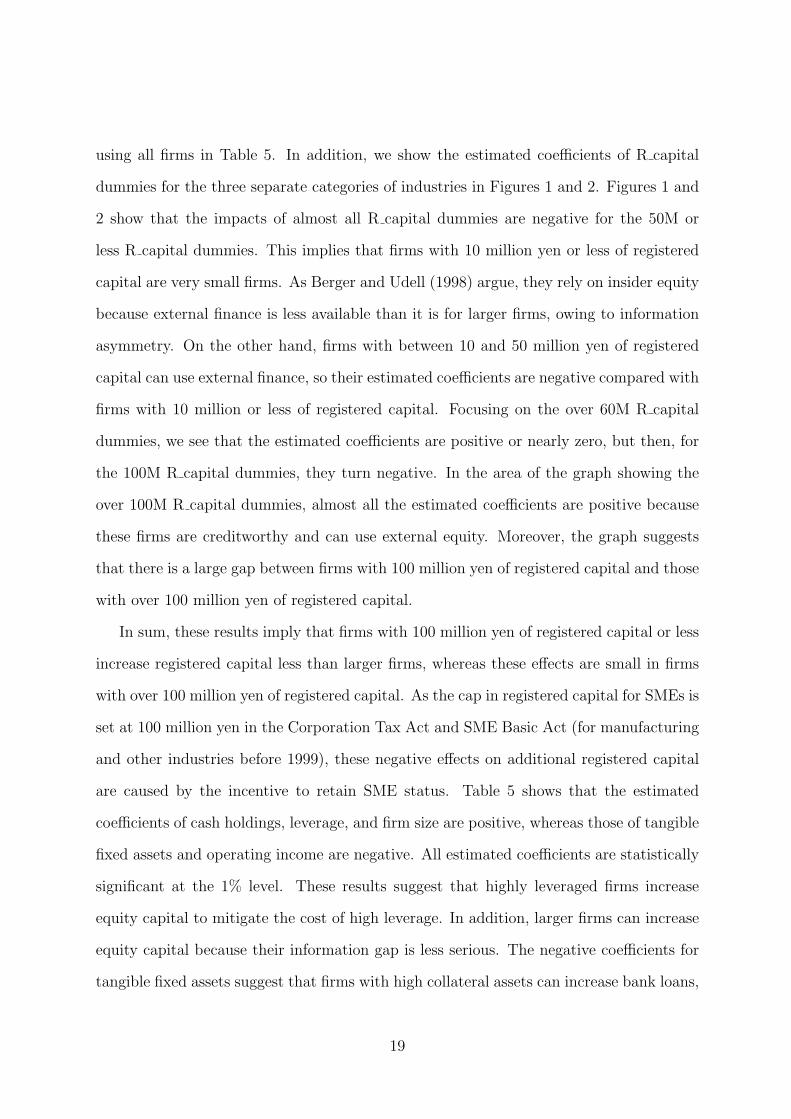
using all firms in Table 5. In addition, we show the estimated coefficients of R capital
dummies for the three separate categories of industries in Figures 1 and 2. Figures 1 and
2 show that the impacts of almost all R capital dummies are negative for the 50M or
less R capital dummies. This implies that firms with 10 million yen or less of registered
capital are very small firms. As Berger and Udell (1998) argue, they rely on insider equity
because external finance is less available than it is for larger firms, owing to information
asymmetry. On the other hand, firms with between 10 and 50 million yen of registered
capital can use external finance, so their estimated coefficients are negative compared with
firms with 10 million or less of registered capital. Focusing on the over 60M R capital
dummies, we see that the estimated coefficients are positive or nearly zero, but then, for
the 100M R capital dummies, they turn negative. In the area of the graph showing the
over 100M R capital dummies, almost all the estimated coefficients are positive because
these firms are creditworthy and can use external equity. Moreover, the graph suggests
that there is a large gap between firms with 100 million yen of registered capital and those
with over 100 million yen of registered capital.
In sum, these results imply that firms with 100 million yen of registered capital or less
increase registered capital less than larger firms, whereas these effects are small in firms
with over 100 million yen of registered capital. As the cap in registered capital for SMEs is
set at 100 million yen in the Corporation Tax Act and SME Basic Act (for manufacturing
and other industries before 1999), these negative effects on additional registered capital
are caused by the incentive to retain SME status. Table 5 shows that the estimated
coefficients of cash holdings, leverage, and firm size are positive, whereas those of tangible
fixed assets and operating income are negative. All estimated coefficients are statistically
significant at the 1% level. These results suggest that highly leveraged firms increase
equity capital to mitigate the cost of high leverage. In addition, larger firms can increase
equity capital because their information gap is less serious. The negative coefficients for
tangible fixed assets suggest that firms with high collateral assets can increase bank loans,
19

so they increase their additional equity less than do firms with fewer collateral assets.
5.2 Changes in Requirements under the SME Basic Act
In the previous subsection, we show that firms increase registered capital less if a firm’s
registered capital is 100 million yen or less. We interpret this as indicating that firms
increase their registered capital less to remain within the SME requirements and retain
their SME status. However, the results could also be interpreted as indicating that it
is difficult for firms with 100 million yen or less of registered capital to increase their
registered capital because they are SMEs that face serious information asymmetry with
investors. Therefore, we conduct another test focusing on an exogenous event, which
is the change in the definition of SMEs in the SME Basic Act. If SMEs limit their
registered capital to remain within the SME requirements, rather than being because of
information asymmetry, they will increase their registered capital after the relaxation of
these constraints following revision of the SME Basic Act.
Table 6 shows the estimation results for treatment1. We limit observations to firms
with 100 million or less of registered capital at the beginning of the fiscal year. Columns
(1) and (2) show the estimation results for policy, which has a value of one if the year is
after FY2000. To check robustness, we also show the results for the policy variable that
has a value of one if the year is 1999. Column (1) shows the estimation results of the
probit estimation using the additional R capital dummy as a dependent variable. The
estimated coefficient of treatment1 × policy is positive and statistically significant at the
1% level, implying that treated firms increase their registered capital more after the change
in the cap on registered capital that occurred under the SME Basic Act. The estimated
coefficient of treatment1 × R capital gap1 is positive and statistically significant at the
1% level. This suggests that treated firms are less likely to increase registered capital if
their registered capital is close to the cap before the change in the SME Basic Act. On the
other hand, the estimated coefficient of treatment1 × R capital gap1 × policy is negative
20
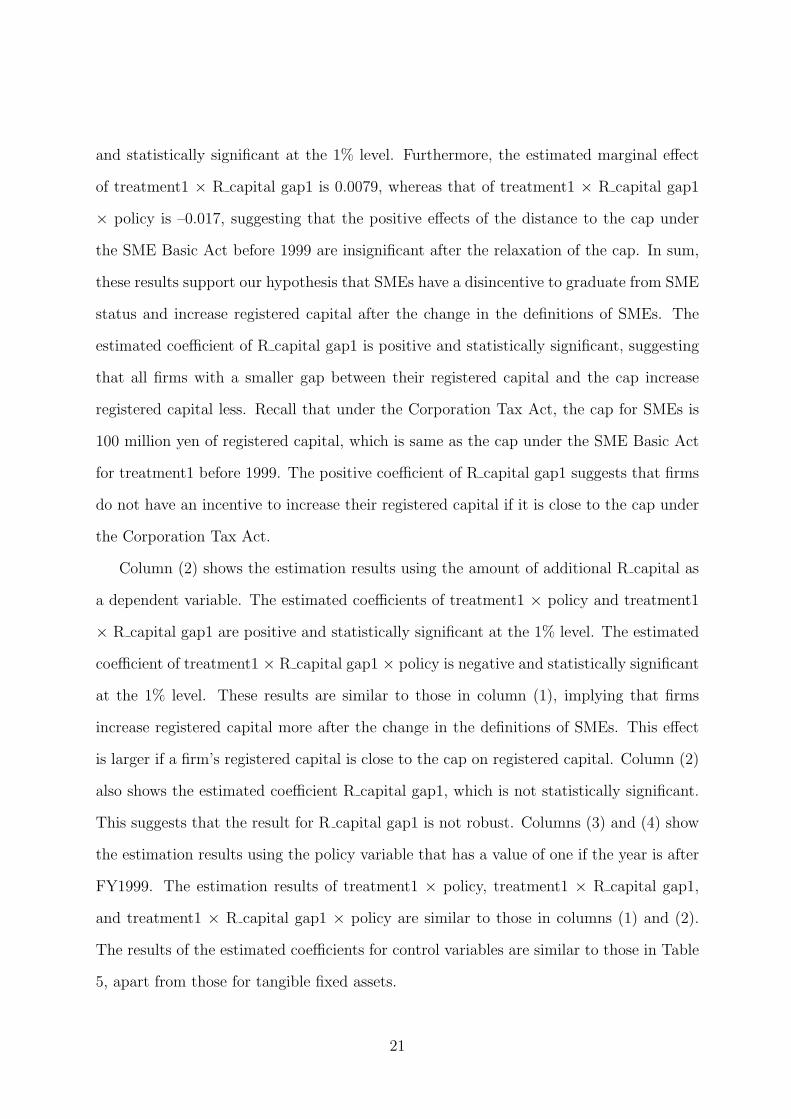
and statistically significant at the 1% level. Furthermore, the estimated marginal effect
of treatment1 × R capital gap1 is 0.0079, whereas that of treatment1 × R capital gap1
× policy is –0.017, suggesting that the positive effects of the distance to the cap under
the SME Basic Act before 1999 are insignificant after the relaxation of the cap. In sum,
these results support our hypothesis that SMEs have a disincentive to graduate from SME
status and increase registered capital after the change in the definitions of SMEs. The
estimated coefficient of R capital gap1 is positive and statistically significant, suggesting
that all firms with a smaller gap between their registered capital and the cap increase
registered capital less. Recall that under the Corporation Tax Act, the cap for SMEs is
100 million yen of registered capital, which is same as the cap under the SME Basic Act
for treatment1 before 1999. The positive coefficient of R capital gap1 suggests that firms
do not have an incentive to increase their registered capital if it is close to the cap under
the Corporation Tax Act.
Column (2) shows the estimation results using the amount of additional R capital as
a dependent variable. The estimated coefficients of treatment1 × policy and treatment1
× R capital gap1 are positive and statistically significant at the 1% level. The estimated
coefficient of treatment1 × R capital gap1 × policy is negative and statistically significant
at the 1% level. These results are similar to those in column (1), implying that firms
increase registered capital more after the change in the definitions of SMEs. This effect
is larger if a firm’s registered capital is close to the cap on registered capital. Column (2)
also shows the estimated coefficient R capital gap1, which is not statistically significant.
This suggests that the result for R capital gap1 is not robust. Columns (3) and (4) show
the estimation results using the policy variable that has a value of one if the year is after
FY1999. The estimation results of treatment1 × policy, treatment1 × R capital gap1,
and treatment1 × R capital gap1 × policy are similar to those in columns (1) and (2).
The results of the estimated coefficients for control variables are similar to those in Table
5, apart from those for tangible fixed assets.
21

Table 7 shows the estimation results using treatment2. Definitions of dependent and
control variables in each column are the same as those in Table 6. We limit observations
to firms with registered capital of 30 million yen or less at the beginning of the fiscal year,
which satisfy the requirements for registered capital under the SME Basic Act before
1999. Although the level of the cap for treatment1 and treatment2 is different under
the SME Basic Act, the estimation results are similar to those in Table 6. The estimated
coefficients of treatment2 × policy and treatment2 × R capital gap2 are positive and those
of treatment2 × R capital gap2 × policy are negative, and all are statistically significant
at the 1% level. These suggest that treated firms increase their registered capital less
before the relaxation of the cap. In particular, these effects are larger for treated firms
with registered capital that is close to the cap. After relaxing the cap in 1999, this effect
is weakened. This implies that the cap set in the definitions of SMEs under the SME
Basic Act is a significant constraint on firms’ additional equity capital.
Table 8 shows the estimation results using treatment3. We limit observations to firms
that satisfy the requirement for registered capital under the SME Basic Act before 1999
(firms with 10 million yen or less of registered capital at the beginning of the fiscal year).
The definitions of dependent and control variables are the same as those in Table 6.
Similarly to the results in Tables 6 and 7, the estimated coefficients of treatment3 ×
policy and treatment3 × R capital gap3 are positive and those of treatment3 × R capital
gap3 × policy are negative. These coefficients are statistically significant at the 1% level.
These results suggest that the estimated results for the treatment and registered capital
gap are robust.
5.3 Effects of Additional Equity on Growth
5.3.1 Asset growth
Table 9 shows the estimation results for equation (3) using asset growth as a dependent
variable. Equation (4) in column (1) is estimated using variables in column (1) of Table 5;
22

that in column (2) is estimated using variables in column (1) in Table 6; that in column (3)
is estimated using variables in column (1) in Table 7; and that in column (4) is estimated
using variables in column (1) in Table 8. Estimated coefficients in equation (4) are similar
to estimated results of each probit model.
Estimated results in Table 9 show that the estimated coefficients of the additional
registered capital dummy are positive and statistically significant at the 1% level. These
results are robust because we obtain similar results if we employ different variables in
equation (4). Estimated ρ is positive and statistically significant at the 1% level; the
assumption of corr(νi, πi) = 0 is therefore supported.
The estimated coefficients of cash holdings are positive and statistically significant at
the 1% level. These results suggest that firms with high liquidity increase firm size more.
The estimated coefficients of leverage are negative and statistically significant at the 1 or
5% level. Because highly leveraged firms are generally financially distressed, the perfor-
mance of firms is lower if leverage is high. The coefficients of tangible assets are negative
and statistically significant at the 1% level. Tangible asset is a proxy for collateral asset.
We predict that the effects of tangible assets are positive on firm performance because
collateral assets mitigate credit constraint for small businesses. However, this prediction is
not supported in the results of Table 9. The estimated coefficients of operating income are
positive and statistically significant at the 1% level. Because profitable firms have more
good investment opportunities, they increase more assets. The estimated coefficients of
firm size are negative and statistically significant at the 1% level.
5.3.2 Debt growth
Table 10 shows the estimation results for equation (3) using debt growth as a dependent
variable. The variables in the first-stage equation in each column are the same as those
in Table 9. The estimated coefficients of the additional registered capital dummy are
positive in column (1) and negative in columns (2), (3), and (4). The coefficients are
23

all statistically significant at the 1% level. The magnitude of the coefficients becomes
larger as the column numbers become smaller, whereas firm size (proxied by the level of
registered capital) becomes smaller as the column numbers become larger. This indicates
that the effects of equity issues on debt finance are positive for larger firms but negative
for smaller firms. This implies that the relaxation of the registered capital constraint
results in lower leverage for smaller firms. For larger firms, equity issues and debt finance
are complements.
5.3.3 Distressed firms
To investigate the effects of additional equity more precisely, we focus on two particular
cases, distressed firms and industries with high volatility. First, we describe the estimation
results using the subsample of distressed firms.
According to the trade-off theory of capital structure, the bankruptcy cost is high
if firms use high levels of debt finance. Therefore, highly leveraged firms might not
achieve an optimal capital structure. If the registered capital constraint is significant,
firms cannot issue new equity without losing their SME status. Consequently, they face
difficulties in adjusting the leverage level to the target. In addition, because of the debt
overhang problem, distressed firms face difficulties in financing investment opportunities
using bank loans. To mitigate this credit constraint, they need to use equity to finance
their investment opportunities. However, under the registered capital constraint, finan-
cially distressed firms do not issue equity in order to keep their SME status.
In sum, we predict that financially distressed firms will increase their additional regis-
tered equity after the relaxation of the registered capital requirement, instead of decreasing
their debt finance, whereas nondistressed firms will not decrease debts. Following Opler
and Titman (1994), we use dummy variables to indicate whether a firm’s leverage is in
the top two deciles of its industry in a particular year as a proxy of financial distress
(hereafter, we refer to the variable as the Distress dummy). Table 11 shows the estimated
24

effects of additional registered capital on total asset growth (Panel A) and total debt
growth (Panel B) as dependent variables using the treatment effects model. We divide
the sample into two subsamples, financially distressed firms (distress=1) and nonfinan-
cially distressed firms (distress=0). In the first-stage equation, we use the same variables
as those in Tables 9 and 10. In Panel A, the estimated coefficient of additional registered
capital is positive and statistically significant at the 1% level for both subsamples of firms.
This implies that distressed and nondistressed firms increase their assets. On the other
hand, the estimation effects for debt growth are mixed. Panel B shows that the estimated
coefficients of additional registered capital are all negative and statistically significant at
the 1% level for financially distressed firms. On the other hand, if we focus on nonfi-
nancially distressed firms, the coefficient is negative only in column (4). Additionally, in
column (4), the negative magnitude of the coefficients is larger for financially distressed
firms. These results support the fact that financially distressed firms decrease their debts
after increasing their equity. As firms increase additional equity after the relaxation of
the registered capital requirement, the change of requirements for SMEs has some effects
on the adjustment of the capital structure by financially distressed firms.
5.3.4 Earnings volatility
As Titman and Wessels (1988) show, the volatility of earnings decreases the optimal level
of leverage. This is because lenders are paid only contractual interest when borrowers earn
high cash flows, even though the credit risk is high. Therefore, lenders do not offer credit
to firms with high volatility. Instead, equity providers prefer to finance high risk, high
return investments, so the optimal leverage level is lower. However, under the registered
capital constraint, firms finance investments using debt even if equity issues are optimal.
Therefore, we expect that, after the relaxation of the requirement, firms with high earning
volatility will decrease debts by increasing additional equity. We test this hypothesis by
dividing the sample into industries with high volatility and low volatility.
25

In this paper, we calculate earnings volatility (defined as the standard deviation of
operating incomes to total assets using data of the past 10 years)13 in each year. Our
database includes all large firms (firms with capital of one billion yen or more), so we
can calculate earnings volatility for many large firms. However, the earnings volatility for
smaller firms cannot be calculated because our data do not contain panel data for smaller
firms. Therefore, we use industry earnings volatility, calculated using the subsample of
large firms. Industry earnings volatility is defined as the median value of the earnings
volatility of large firms in the medium category in the industrial classification. We use
industry earnings volatility (which is industry level data) as a proxy for the earnings
volatility of a firm.
To test our hypothesis, we divide the sample into two subsamples, firms with industry
earnings volatility in the top tertile (high volatility) and those with volatility in the bottom
tertile (low volatility). We predict that firms with high volatility will decrease debts by
increasing equity after the relaxation of the registered capital constraint.
The estimation results are shown in Table 12. In both subsamples, i.e., for firms with
high and low volatility, the coefficients of additional registered capital are positive and
statistically significant at the 1% level (Panel A). The magnitude of the coefficients is
larger for firms with high volatility, indicating that the effects on asset growth are large
for those firms. Focusing on the effects on total debt growth, we see that the estimated
coefficients of additional registered capital are negative for firms with high volatility. This
implies that firms decrease debts if they increase registered capital. On the other hand,
in Panel B, the estimated coefficients of additional registered capital are positive, with
the exception of those in column (4) (although they are not statistically significant in
column (3)). This suggests that the subsample of low volatility firms, in contrast to the
high volatility firms, do not decrease debts when they increase their registered capital.
In sum, these estimation results support our hypothesis that firms with high volatility
13This definition is used in Titman and Wessels (1988).
26
decrease debts after the relaxation of the registered capital requirements allow them to
adjust their capital structure.
5.4 Discussion
5.4.1 Policy dummy
The coefficients of the interaction variable for the treatment dummies for FY1999 and
FY2000 and the policy variables are positive and statistically significant in all tables.
However, we do not test whether these positive effects exist for policy dummy variables
for other fiscal years. To test the other years around the changing of the SME Basic
Act, we reestimate equation (2) including policy dummies for five fiscal years before and
after the pseudo shock year. If the years around the change in the SME Basic Act have
positive effects, the estimation results support our hypothesis for shock year dummies
close to FY1999.
Table 13 shows the estimation results using policy dummies from FY1996 to FY2002.
Panel A shows the estimation results using treatment1, Panel B shows those using treat-
ment2, and Panel C shows those using treatment3. In all panels, the magnitude of coeffi-
cients of treatment×policy, treatment×R capital gap, and treatment×R capital gap×policy
is large around FY1999. However, focusing on FY1996 and FY2002, we see that those
estimated coefficients are statistically insignificant or their magnitude is small. In sum,
only the estimation results for the years around FY1999 support our hypothesis.
5.4.2 Other factors?
We investigate the effects of the SME Basic Act by using year dummies for FY1999 or
2000. However, the estimation results may be measuring the effects of other events, not
the change in the SME Basic Act. We now consider whether other events have affected
our estimated results. First, Hokkaido Takushoku Bank and Yamaichi Securities, two
of the largest financial institutions in Japan, went bankrupt in November 1997. After
27

the collapse of these financial institutions, many papers (for example Kuttner and Posen,
2001) argue that a credit crunch took place and credit availability worsened in small
businesses around 1999. Therefore, this shock is likely to have had some impact on the
financial activities and firm performance of small businesses in Japan. However, this shock
is common among all industries; therefore, heterogeneous responses across manufacturing,
wholesale, retail, and service industries are not explainable by the effects of the shock.
Second, related to the first point, the total value of public credit guarantees increased
substantially after October 1998 to mitigate the negative effects of the credit crunch,
which was an important event for small businesses in Japan. As Uesugi et al. (2010)
argue, the public credit guarantee program during the shock enhanced credit availability
for small businesses. If credit-guaranteed loans are a substitute for new equity issues, the
additional registered capital decreases after the increase in the total value of public credit
guarantees. However, small businesses in all industries can use this program; therefore,
the commencement of this program does not have any effects on the treatment dummy.
6 Conclusion
In this paper, we have investigated whether firms have a disincentive to graduate from
being SMEs to become large firms. To test this hypothesis, we employed two empirical
strategies. First, we showed that firms with 100 million yen of registered capital are less
likely to increase their registered capital. As SMEs are defined under the Corporation
Tax Act and the SME Basic Act as firms with registered capital of 100 million yen or less,
such firms have an incentive to meet the SME requirements and retain their SME status.
Second, we showed that, after the relaxation of the definitions of SMEs under the SME
Basic Act, firms were more likely to increase their registered capital. This effect is larger
if a firm’s registered capital is close to the cap set in the SME definition. This implies
that the registered capital requirement is an effective constraint on the accumulation of
additional equity capital.
28

We also showed that additional registered capital has positive effects on firm growth
(in terms of the growth rate of a firm’s total assets). As the requirements for registered
capital in the definitions of SMEs have negative effects on additional registered capital,
the SME requirements impede firm growth for SMEs.
Our study has important implications for SME policies. As noted, SME policies
can be important for mitigating market failure. However, the menu of SME policies
adopted in Japan impedes firm growth. Governments should therefore be cautious about
implementing an excessive range of policies to support SMEs.
29
References
Acs, Z., Szerb, L., March 2007. Entrepreneurship, Economic Growth and Public Policy.
Small Business Economics 28 (2), 109–122.
Berger, A. N., Udell, G. F., 1998. The economics of small business finance: The roles of
private equity and debt markets in the financial growth cycle. Journal of Banking &
Finance 22, 613–673.
Craig, B. R., Jackson, W. E., Thomson, J. B., 2007. Small firm finance, credit rationing,
and the impact of sba-guaranteed lending on local economic growth. Journal of Small
Business Management 45 (1), 116–132.
Garcıa-Santana, M., Pijoan-Mas, J., 2014. The reservation laws in India and the misallo-
cation of production factors. Journal of Monetary Economics 66, 193 – 209.
Garicano, L., Lelarge, C., Reenen, J. V., 2016. Firm Size Distortions and the Productivity
Distribution: Evidence from France. American Economic Review 106 (11), 3439–79.
Goto, Y., 2014. Macro-performance of Small and Medium Enterprises (in Japanese).
Nikkei Publishing Inc., Tokyo.
Gourio, F., Roys, N., 2014. Size-dependent regulations, firm size distribution, and reallo-
cation. Quantitative Economics 5 (2), 377–416.
Guner, N., Ventura, G., Xu, Y., 2008. Macroeconomic implications of size-dependent
policies. Review of Economic Dynamics 11 (4), 721 – 744.
Guner, N., Ventura, G., Yi, X., August 2006. How costly are restrictions on size? Japan
and the World Economy 18 (3), 302–320.
Honjo, Y., Harada, N., 2006. SME policy, financial structure and firm growth: Evidence
from Japan. Small Business Economics 27 (4), 289–300.
30

Kang, J. W., Heshmati, A., 2008. Effect of credit guarantee policy on survival and per-
formance of smes in republic of Korea. Small Business Economics 31 (4), 445–462.
Kuttner, K. N., Posen, A. S., 2001. The great recession: Lessons for macroeconomic policy
from Japan. Brookings Papers on Economic Activity 64 (2001-2), 93–186.
Mankiw, N. G., August 1986. The allocation of credit and financial collapse. Quarterly
Journal of Economics 101 (3), 455–70.
OECD, 2013. SME and entrepreneurship financing: The role of credit guarantee schemes
and mutual guarantee societies in supporting finance for small and medium-sized enter-
prises,Final Report, Paris: Centre for Entrepreneurship, SMEs and Local Development.
OECD, 2016. Japan: Boosting growth and well-being in an ageing society.
Oh, I., Lee, J.-D., Heshmati, A., Choi, G.-G., 2009. Evaluation of credit guarantee policy
using propensity score matching. Small Business Economics 33 (3), 335–351.
Ono, A., Uesugi, I., Yasuda, Y., 2013. Are lending relationships beneficial or harmful for
public credit guarantees? Evidence from Japan’s emergency credit guarantee program.
Journal of Financial Stability 9 (2), 151 – 167.
Opler, T. C., Titman, S., 1994. Financial distress and corporate performance. Journal of
Finance 49 (3), 1015–40.
Ou, C., Haynes, G. W., 2006. Acquisition of additional equity capital by small firms –
findings from the national survey of small business finances. Small Business Economics
27 (2), 157–168.
Storey, D. J., 1994. Understanding the Small Business Sector. Thomson Learning, London.
Storey, D. J., 2008. Entrepreneurship and sme policy, World Entrepreneurship Forum
2008 Edition, available at:
http://www.world-entrepreneurship-forum.com/Publications/Articles .
31

Titman, S., Wessels, R., 1988. The determinants of capital structure choice. The Journal
of Finance 43 (1), 1–19.
Uesugi, I., Sakai, K., Yamashiro, G. M., 2010. The effectiveness of public credit guarantees
in the Japanese loan market. Journal of the Japanese and International Economies
24 (4), 457–480.
32

Tab
le1:
Lis
tof
Majo
rSM
EPol
icie
sin
Jap
an
Managem
ent
Support
Sta
rt-u
ps
and
ven
ture
sA
ssis
tsth
ose
pla
nnin
gto
start
abusi
nes
sor
ven
ture
ow
ner
str
yin
gto
impro
ve
thei
roper
ations
infinanci
ng
and
obta
inin
gre
levant
info
rmation.
Busi
nes
sin
novation
Ass
ists
SM
Es
under
goin
gbusi
nes
sin
novation
infinanci
ng,handling
taxes
,and
cultiv
ating
mark
ets.
New
collabora
tion
Support
sco
llabora
tion
bet
wee
nSM
Es
toen
ter
new
are
as
ofbusi
nes
sby
pro
vid
ing
subsi
die
s,advic
e,and
financi
ng
ass
ista
nce
.B
usi
nes
sre
vitaliza
tion
Support
sSM
Es
inth
eir
effort
sto
revitalize
thei
rbusi
nes
sth
rough
the
SM
ER
evitaliza
tion
Support
Com
mitte
e.E
mplo
ym
ent
and
hum
an
reso
urc
esSupport
sSM
Es
with
hum
an
reso
urc
esdev
elopm
ent
and
the
reso
lution
of
busi
nes
sch
allen
ges
by
imple
men
ting
the
Sm
all
and
Med
ium
-siz
edE
nte
rpri
seC
onsu
ltants
syst
em,offer
ing
train
ing,and
dis
patc
hin
gex
per
ts.
Glo
baliza
tion
Pro
vid
esin
form
ation
and
advic
eto
hel
pSM
Es
tom
ove
pro
duct
ion
over
seas
or
find
mark
ets
abro
ad.
Tra
de
pra
ctic
esand
public
pro
cure
-m
ent
Pro
mote
sfa
irsu
bco
ntr
act
ing
pra
ctic
esand
the
dev
elopm
ent
ofsm
all
and
med
ium
-siz
edsu
bco
ntr
act
ors
and
ther
eby
incr
ease
sth
eopport
unity
for
SM
Es
tow
inco
ntr
act
s.B
usi
nes
sst
ability
Ass
ists
SM
Es
inm
ain
tain
ing
stable
oper
ations
by
support
ing
them
duri
ng
bankru
ptc
y,new
pandem
icin
fluen
za,and
eart
hquakes
and
oth
ernatu
ral
dis
ast
ers,
as
wel
las
by
ass
isting
them
todev
elop
busi
nes
sco
ntinuity
pla
ns.
Mutu
alaid
syst
emH
elps
small
com
panie
sto
pre
pare
for
busi
nes
scl
osu
reand
retire
men
t,and
SM
Es
topre
pare
for
the
bankru
ptc
yofth
eir
majo
rcu
stom
ers.
Sm
all
busi
nes
ses
Pro
vid
esm
anager
ialand
financi
alsu
pport
tosm
all
busi
nes
sesw
ith
20
orfe
wer
emplo
yee
s(fi
ve
orfe
wer
forth
ose
inth
eco
mm
erce
orse
rvic
ese
ctor)
.Sm
all
and
med
ium
manufa
cture
rsSupport
sR
&D
and
hum
an
reso
urc
esdev
elopm
ent
at
SM
Es
with
key
manufa
cturi
ng
tech
nolo
gie
s.Sel
ects
“300
of
Japan’s
Exci
ting
Monozu
kuri
(Manufa
cturi
ng)
SM
Es.
”Tec
hnolo
gic
al
innovation,
IT,
and
en-
ergy
effici
ency
Ass
ists
SM
Es
com
mitte
dto
tech
nolo
gic
aldev
elopm
ent,
ITutiliza
tion,and
hig
her
ener
gy
effici
ency
by
pro
vid
ing
subsi
die
s,financi
alass
ista
nce
,and
rele
vant
info
rmation.
Inte
llec
tualpro
per
tySupport
sSM
Es
with
inte
llec
tualpro
per
tyst
rate
gie
sby
imple
men
ting
mea
sure
sto
pro
tect
inte
llec
tualpro
per
tyand
mea
sure
sto
com
bat
dam
age
cause
dby
counte
rfei
ting.
SM
EA
ssis
tance
Cen
ters
Dis
patc
hes
exper
tsto
ass
ist
SM
Es
inaddre
ssin
gdiffi
cult
or
spec
ialize
dbusi
nes
sch
allen
ges
(e.g
.,la
unch
ofnew
oper
ations
or
busi
nes
ssu
cces
sion)
and
oth
erw
ise
hel
ps
SM
Es
dir
ectly
or
via
support
inst
itutions.
Fin
anci
alSupport
Safe
ty-n
etguara
nte
epro
gra
mSupport
sSM
Es
whose
busi
nes
sst
ability
isth
reate
ned
by
exte
rnalfa
ctors
(e.g
.,a
majo
rcu
stom
er’s
rest
rict
edoper
ations
or
applica
tion
for
reha-
bilitation
pro
cedure
s,th
eim
pact
ofa
dis
ast
er,or
the
failure
ofth
em
ain
bank)
by
makin
gadditio
nalcr
edit
guara
nte
esavailable
.Safe
ty-n
etlo
ans
Makes
loans
toSM
Es
tem
pora
rily
faci
ng
cash
flow
pro
ble
ms
ow
ing
toa
radic
alch
ange
inth
ebusi
nes
sen
vir
onm
ent,
the
bankru
ptc
yof
am
ajo
rcu
stom
er,or
the
stre
am
linin
gofth
em
ain
bank.
Fis
calSupport
Taxation
Giv
esin
form
ation
and
advic
eon
vari
ous
tax
mea
sure
sto
support
SM
Es.
Acc
ounting
Giv
esin
form
ation
and
advic
eon
“SM
Eacc
ounting,”
whic
hhel
ps
SM
Es
toen
hance
thei
rca
pability
toanaly
zem
anagem
ent,
ensu
refinanci
ng,and
incr
ease
ord
erin
take.
Com
panie
sA
ctG
ives
info
rmation
and
advic
eon
the
new
Com
panie
sA
ct,w
hic
hadditio
nally
incl
udes
syst
ems
that
bri
ng
signifi
cant
ben
efits
toSM
Es,
such
as
the
acc
ounting
advis
ersy
stem
.B
usi
nes
ssu
cces
sion
Giv
esin
form
ation
and
advic
eon
mea
sure
sto
support
SM
Es’
smooth
busi
nes
ssu
cces
sion.
Com
mer
ceand
Reg
ionalSupport
Rev
italiza
tion
ofco
mm
erce
Support
seff
ort
sto
impro
ve
the
att
ract
iven
ess
ofsm
all
and
med
ium
mer
chants
,sh
oppin
gdis
tric
ts,and
city
cente
rs.
Reg
ionalin
dust
ries
Invig
ora
tes
regio
nalin
dust
ries
,su
chas
loca
lly
base
din
dust
ries
and
traditio
nalhandic
raft
indust
ries
,by
pro
vid
ing
subsi
die
sand
low
-inte
rest
loans.
Collabora
tion
bet
wee
nagri
culture
,co
mm
erce
,and
indust
ryC
om
pre
hen
sivel
yass
ists
busi
nes
sact
ivitie
sco
nduct
edby
org
anic
part
ner
ship
sbet
wee
nSM
Es
and
those
engaged
inagri
culture
/fo
rest
ry/fish
erie
sth
rough
the
effec
tive
use
ofth
eir
busi
nes
sre
sourc
es.
“M
eet
and
Exper
ience
Reg
ional
At-
tract
iven
ess”
cam
paig
nA
ctiv
ely
support
sand
incr
ease
sth
epublici
tyfo
ratt
ract
ive
regio
nalpro
duct
s.
Sour
ce:
Web
site
ofth
eSm
allan
dM
ediu
mE
nter
pris
eA
genc
y(h
ttp:
//w
ww
.chu
sho.
met
i.go.
jp/s
me
engl
ish/
outl
ine/
04/0
1.ht
ml)
.N
ote:
Thi
sta
ble
show
sth
elis
tof
SME
polic
ies
impl
emen
ted
byth
eM
inis
try
ofE
cono
my,
Tra
dean
dIn
dust
ry(M
ET
I)in
Japa
n.
33
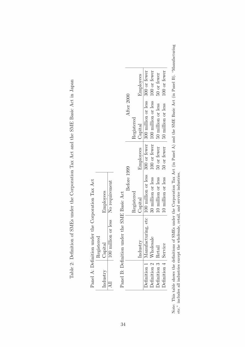
Tab
le2:
Defi
nit
ion
ofSM
Es
under
the
Cor
por
atio
nTax
Act
and
the
SM
EB
asic
Act
inJap
an
Pan
elA
:D
efinit
ion
under
the
Cor
por
atio
nTax
Act
Reg
iste
red
Indust
ryC
apit
alE
mplo
yees
All
100
million
orle
ssN
ore
quir
emen
t
Pan
elB
:D
efinit
ion
under
the
SM
EB
asic
Act
Bef
ore
1999
Aft
er20
00R
egis
tere
dR
egis
tere
dIn
dust
ryC
apit
alE
mplo
yees
Cap
ital
Em
plo
yees
Defi
nit
ion
1M
anufa
cturi
ng,
etc
100
million
orle
ss30
0or
few
er30
0m
illion
orle
ss30
0or
few
erD
efinit
ion
2W
hol
esal
e30
million
orle
ss10
0or
few
er10
0m
illion
orle
ss10
0or
few
erD
efinit
ion
3R
etai
l10
million
orle
ss50
orfe
wer
50m
illion
orle
ss50
orfe
wer
Defi
nit
ion
4Ser
vic
e10
million
orle
ss50
orfe
wer
50m
illion
orle
ss10
0or
few
er
Not
e:T
his
tabl
esh
ows
the
defin
itio
nsof
SME
sun
der
the
Cor
pora
tion
Tax
Act
(in
Pan
elA
)an
dth
eSM
EB
asic
Act
(in
Pan
elB
).“M
anuf
actu
ring
etc.
”in
clud
esal
lin
dust
ries
exce
ptth
ew
hole
sale
,re
tail,
and
serv
ice
indu
stri
es.
34
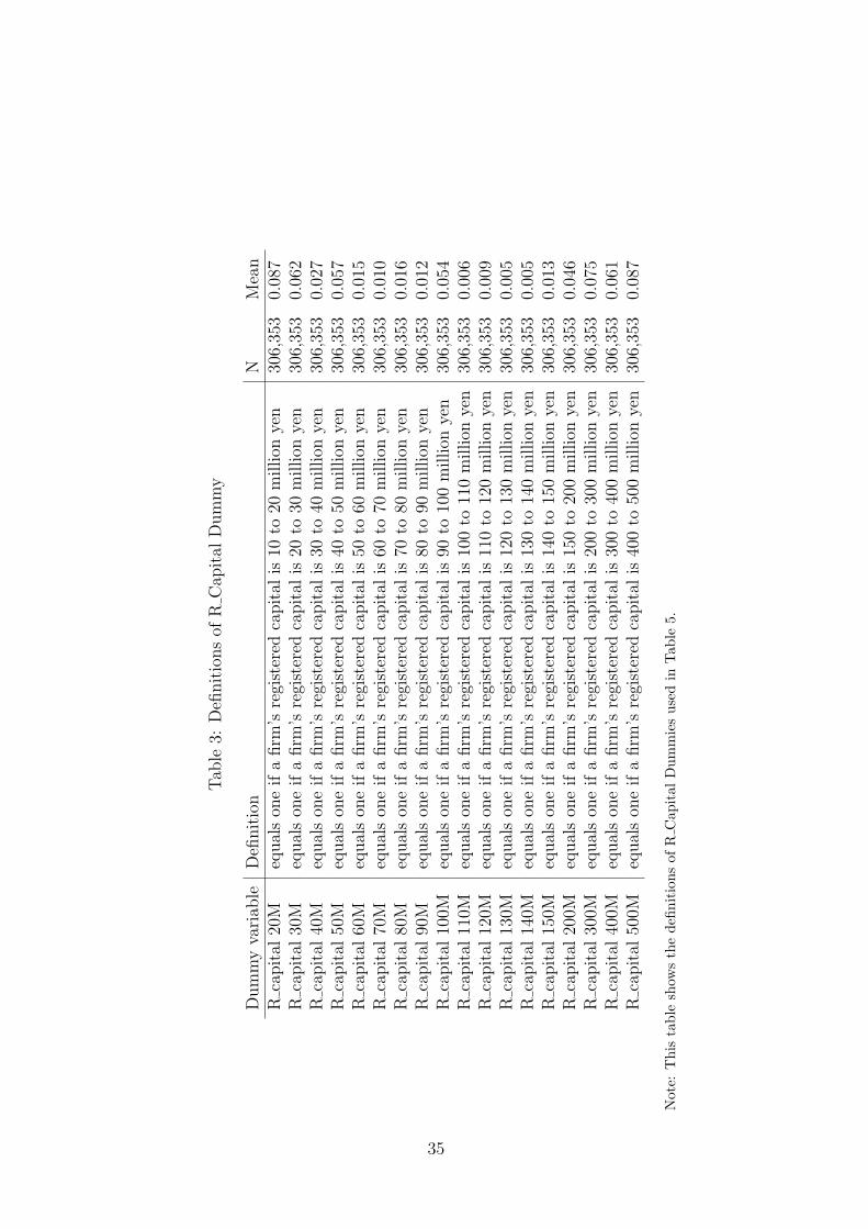
Tab
le3:
Defi
nit
ions
ofR
Cap
ital
Dum
my
Dum
my
vari
able
Defi
nit
ion
NM
ean
Rca
pit
al20
Meq
ual
son
eif
afirm
’sre
gist
ered
capit
alis
10to
20m
illion
yen
306,
353
0.08
7R
capit
al30
Meq
ual
son
eif
afirm
’sre
gist
ered
capit
alis
20to
30m
illion
yen
306,
353
0.06
2R
capit
al40
Meq
ual
son
eif
afirm
’sre
gist
ered
capit
alis
30to
40m
illion
yen
306,
353
0.02
7R
capit
al50
Meq
ual
son
eif
afirm
’sre
gist
ered
capit
alis
40to
50m
illion
yen
306,
353
0.05
7R
capit
al60
Meq
ual
son
eif
afirm
’sre
gist
ered
capit
alis
50to
60m
illion
yen
306,
353
0.01
5R
capit
al70
Meq
ual
son
eif
afirm
’sre
gist
ered
capit
alis
60to
70m
illion
yen
306,
353
0.01
0R
capit
al80
Meq
ual
son
eif
afirm
’sre
gist
ered
capit
alis
70to
80m
illion
yen
306,
353
0.01
6R
capit
al90
Meq
ual
son
eif
afirm
’sre
gist
ered
capit
alis
80to
90m
illion
yen
306,
353
0.01
2R
capit
al10
0Meq
ual
son
eif
afirm
’sre
gist
ered
capit
alis
90to
100
million
yen
306,
353
0.05
4R
capit
al11
0Meq
ual
son
eif
afirm
’sre
gist
ered
capit
alis
100
to11
0m
illion
yen
306,
353
0.00
6R
capit
al12
0Meq
ual
son
eif
afirm
’sre
gist
ered
capit
alis
110
to12
0m
illion
yen
306,
353
0.00
9R
capit
al13
0Meq
ual
son
eif
afirm
’sre
gist
ered
capit
alis
120
to13
0m
illion
yen
306,
353
0.00
5R
capit
al14
0Meq
ual
son
eif
afirm
’sre
gist
ered
capit
alis
130
to14
0m
illion
yen
306,
353
0.00
5R
capit
al15
0Meq
ual
son
eif
afirm
’sre
gist
ered
capit
alis
140
to15
0m
illion
yen
306,
353
0.01
3R
capit
al20
0Meq
ual
son
eif
afirm
’sre
gist
ered
capit
alis
150
to20
0m
illion
yen
306,
353
0.04
6R
capit
al30
0Meq
ual
son
eif
afirm
’sre
gist
ered
capit
alis
200
to30
0m
illion
yen
306,
353
0.07
5R
capit
al40
0Meq
ual
son
eif
afirm
’sre
gist
ered
capit
alis
300
to40
0m
illion
yen
306,
353
0.06
1R
capit
al50
0Meq
ual
son
eif
afirm
’sre
gist
ered
capit
alis
400
to50
0m
illion
yen
306,
353
0.08
7
Not
e:T
his
tabl
esh
ows
the
defin
itio
nsof
RC
apit
alD
umm
ies
used
inTab
le5.
35

Tab
le4:
Sum
mar
ySta
tist
ics
Var
iable
Nm
ean
sdm
inp1
p50
p99
max
Addit
ional
RC
apit
alD
um
my
306,
353
0.04
60.
210
0.00
00.
000
0.00
01.
000
1.00
0A
mou
nt
ofA
ddit
ional
Rca
pit
al30
6,35
34.
141
46.1
250.
000
0.00
00.
000
100.
000
1500
.000
Tre
atm
ent1
×R
Cap
ital
Gap
121
1,91
52.
600
2.12
90.
000
0.00
03.
932
4.61
54.
615
RC
apit
alG
ap1
211,
915
4.02
61.
169
0.00
00.
000
4.51
14.
615
4.61
5Tre
atm
ent1
211,
915
0.64
60.
478
0.00
00.
000
1.00
01.
000
1.00
0Tre
atm
ent2
×R
Cap
ital
Gap
215
2,99
70.
262
0.85
50.
000
0.00
00.
000
3.43
43.
434
RC
apit
alG
ap2
152,
997
2.85
70.
897
0.00
00.
000
3.04
53.
434
3.43
4Tre
atm
ent2
152,
997
0.09
70.
295
0.00
00.
000
0.00
01.
000
1.00
0Tre
atm
ent3
×R
Cap
ital
Gap
310
7,33
20.
527
0.99
00.
000
0.00
00.
000
2.39
82.
398
RC
apit
alG
ap3
107,
332
1.57
51.
129
0.00
00.
000
2.39
72.
398
2.39
8Tre
atm
ent3
107,
332
0.30
80.
462
0.00
00.
000
0.00
01.
000
1.00
0C
ash
Hol
din
gs30
6,35
30.
180
0.18
40.
000
0.00
00.
122
0.88
21.
000
Lev
erag
e30
6,35
30.
785
0.40
70.
000
0.00
00.
796
2.35
73.
360
Tan
gible
Fix
edA
sset
s30
6,35
30.
339
0.27
10.
000
0.00
00.
286
0.96
72.
200
Oper
atin
gIn
com
e30
6,35
30.
007
0.11
0-0
.709
-0.4
480.
019
0.24
90.
334
Fir
mSiz
e30
6,35
34.
464
4.62
9-1
3.81
6-5
.787
5.99
910
.491
14.3
72Tot
alA
sset
Gro
wth
303,
356
0.02
50.
221
-0.9
93-0
.452
-0.0
030.
932
1.70
6
Not
e:T
his
tabl
esh
ows
the
sum
mar
yst
atis
tics
ofth
eva
riab
les
used
inth
eec
onom
etri
can
alys
is.
36

Table 5: Estimation Results for Effects on Additional Registered Capital
Proxy of Dependent Variable Dummy AmountIndustry All AllR capital 20M -0.0167∗∗∗ -55.4291∗∗∗
(0.001) (4.889)R capital 30M -0.0158∗∗∗ -51.4031∗∗∗
(0.001) (5.666)R capital 40M -0.0085∗∗∗ -19.7155∗∗
(0.002) (7.683)R capital 50M -0.0166∗∗∗ -49.9706∗∗∗
(0.001) (6.187)R capital 60M -0.0053∗ -2.4591
(0.003) (10.066)R capital 70M 0.0062 33.8065∗∗∗
(0.004) (11.383)R capital 80M -0.0078∗∗∗ -11.3949
(0.003) (10.190)R capital 90M -0.0017 15.5089
(0.003) (11.096)R capital 100M -0.0169∗∗∗ -30.2832∗∗∗
(0.001) (6.678)R capital 110M 0.0086∗ 49.4246∗∗∗
(0.005) (14.012)R capital 120M 0.0103∗∗ 59.3763∗∗∗
(0.004) (11.937)R capital 130M 0.0284∗∗∗ 99.7992∗∗∗
(0.006) (14.340)R capital 140M 0.0153∗∗ 64.1389∗∗∗
(0.006) (15.417)
[Continue to the next page]
37

R capital 150M -0.0009 32.8672∗∗∗
(0.003) (10.944)R capital 200M 0.0092∗∗∗ 64.8393∗∗∗
(0.002) (5.818)R capital 300M 0.0124∗∗∗ 77.9329∗∗∗
(0.002) (4.885)R capital 400M 0.0195∗∗∗ 109.0838∗∗∗
(0.002) (5.653)R capital 500M 0.0025∗ 71.2375∗∗∗
(0.001) (5.304)Cash Holdings 0.0135∗∗∗ 48.6720∗∗∗
(0.002) (7.337)Leverage 0.0131∗∗∗ 47.3439∗∗∗
(0.001) (2.848)Tangible Fixed Assets -0.0140∗∗∗ -50.7015∗∗∗
(0.002) (5.524)Operating Income -0.0056∗ -24.4912∗∗
(0.003) (10.928)Year Fixed Effects Yes YesIndustry Fixed Effects Yes YesObservations 306,353 306,353Log-likelihood -54,271 -135,197
Note: This table presents estimates of probit and tobit regressions with the additional R capital dummyand the amount of additional R capital as dependent variables. The additional R capital dummy (shownas “Dummy” in the table) is a dummy variable that has a value of one if registered capital is larger at theend of fiscal year t than it is at the beginning of fiscal year t. Additional R capital (shown as “Amount”in the table) is the difference in registered capital at the end of fiscal year t from that at the beginningof fiscal year t. Definitions of R capital dummies are shown in Table 3. Leverage is defined as the bookvalue of debt divided by the book value of assets at the beginning of fiscal year t. Tangible fixed assetsare defined as the ratio of a firm’s tangible fixed assets to total assets at the beginning of fiscal year t.Cash holdings are defined as the ratio of a firm’s cash holdings to total assets at the beginning of fiscalyear t. Operating incomes are defined as operating income in fiscal year t, normalized by total assets atthe beginning of fiscal year t. Firm size is defined as the natural logarithm of total assets at the beginningof fiscal year t. Seven year dummies from FY1992 to FY2007 and 43 industry dummies are included.The reference year is FY1991. The marginal effects of each variable are shown in this table. Estimatedrobust standard errors are shown in parentheses. The symbols ∗, ∗∗, and ∗∗∗ denote significance at the10%, 5%, and 1% levels.
38

Figure 1: Magnitude of Estimated Marginal Effects of R Capital Dummies on AdditionalR capital dummy, by Industry
−.02
0.0
2.0
4.0
6
R_c
apita
l 20M
R_c
apita
l 30M
R_c
apita
l 40M
R_c
apita
l 50M
R_c
apita
l 60M
R_c
apita
l 70M
R_c
apita
l 80M
R_c
apita
l 90M
R_c
apita
l 100
M
R_c
apita
l 110
M
R_c
apita
l 120
M
R_c
apita
l 130
M
R_c
apita
l 140
M
R_c
apita
l 150
M
R_c
apita
l 200
M
R_c
apita
l 300
M
R_c
apita
l 400
M
R_c
apita
l 500
M
All Manufacturing, etcWholesale Retail and Service
Note: This figure shows the estimated marginal effects of R capital dummies on R capital dummy usingthe probit estimation. The estimated result for all firms is shown in column (1) of Table 5. Other resultsare not reported in any table.
Figure 2: Magnitude of Estimated Coefficients of R Capital Dummies on AdditionalR capital, by Industry
−100
−50
050
100
150
R_c
apita
l 20M
R_c
apita
l 30M
R_c
apita
l 40M
R_c
apita
l 50M
R_c
apita
l 60M
R_c
apita
l 70M
R_c
apita
l 80M
R_c
apita
l 90M
R_c
apita
l 100
M
R_c
apita
l 110
M
R_c
apita
l 120
M
R_c
apita
l 130
M
R_c
apita
l 140
M
R_c
apita
l 150
M
R_c
apita
l 200
M
R_c
apita
l 300
M
R_c
apita
l 400
M
R_c
apita
l 500
M
All Manufacturing, etcWholesale Retail and Service
Note: This figure shows the estimated coefficient of R capital dummies on additional R capital using thetobit estimation. The estimated result for all firms is shown in column (2) of Table 5. Other results arenot reported in any table.
39

Table 6: Estimation Results for the Effects of Changing the Definitions of SMEs on theManufacturing Industry
(1) (2) (3) (4)Dependent Variable ∆R CapitalProxy of Dependent Variable Dummy Amount Dummy AmountPeriod of Policy FY2000 FY2000 FY1999 FY1999Treatment1 × Policy 0.0607∗∗∗ 44.6983∗∗∗ 0.0644∗∗∗ 47.5291∗∗∗
(0.008) (9.491) (0.008) (9.473)Treatment1 × R Capital Gap1 0.0079∗∗∗ 7.5846∗∗∗ 0.0087∗∗∗ 8.2930∗∗∗
(0.001) (1.821) (0.001) (1.893)Treatment1 × R Capital Gap1 -0.0117∗∗∗ -12.3648∗∗∗ -0.0125∗∗∗ -12.9180∗∗∗
× Policy (0.001) (2.153) (0.001) (2.155)R Capital Gap1 0.0039∗∗∗ 0.5967 0.0039∗∗∗ 0.6026
(0.001) (1.051) (0.001) (1.052)Cash Holdings 0.0113∗∗∗ 16.3263∗∗∗ 0.0113∗∗∗ 16.3449∗∗∗
(0.002) (3.874) (0.002) (3.876)Leverage -0.0106∗∗∗ -17.4111∗∗∗ -0.0106∗∗∗ -17.4154∗∗∗
(0.002) (2.914) (0.002) (2.915)Tangible Fixed Assets 0.0153∗∗∗ 24.2394∗∗∗ 0.0153∗∗∗ 24.2549∗∗∗
(0.001) (1.723) (0.001) (1.723)Operating Income -0.0047 -14.2366∗∗∗ -0.0047 -14.3296∗∗∗
(0.003) (4.903) (0.003) (4.905)ln (Total Assets) 0.0013∗∗∗ 2.6508∗∗∗ 0.0013∗∗∗ 2.6554∗∗∗
(0.000) (0.189) (0.000) (0.189)Year Fixed Effects Yes Yes Yes YesIndustry Fixed Effects Yes Yes Yes YesObservations 211,915 211,915 211,915 211,915Log-likelihood -33,662 -75,731 -33,651 -75,726
Note: This table presents estimates of probit and tobit regressions with the additional R capital dummyand the amount of additional R capital as dependent variables. The additional R capital dummy (shownas “Dummy” in the table) is a dummy variable that has a value of one if registered capital is larger atthe end of fiscal year t than at the beginning of fiscal year t. Additional R capital (shown as “Amount”in the table) is the difference in registered capital at the end of fiscal year t from that at the beginningof fiscal year t. Treatment1 has a value of one if firms do not belong to the wholesale, retail, or serviceindustries, and a value of zero otherwise, in order to focus on the change in Definition 1, shown in Table2. Policy has a value of one if the year is after FY2000 in columns (1) and (2), and after FY1999 incolumns (3) and (4). R Capital Gap1 is defined as the natural logarithm of 100 million yen minus afirm’s registered capital at the beginning of fiscal year t. Definitions of other independent variables areshown in the note to Table 5. The marginal effects of each variable are shown in this table. Estimatedrobust standard errors are shown in parentheses. The symbols ∗, ∗∗, and ∗∗∗ denote significance at the10%, 5%, and 1% levels.
40

Table 7: Estimation Results for the Effects of Changing the Definitions of SMEs on theWholesale Industry
(1) (2) (3) (4)Dependent Variable ∆R CapitalProxy of Dependent Variable Dummy Amount Dummy AmountPeriod of Policy FY2000 FY2000 FY1999 FY1999Treatment2 × Policy 0.1369∗∗∗ 42.8303∗∗∗ 0.1579∗∗∗ 47.3516∗∗∗
(0.050) (12.266) (0.053) (12.401)Treatment2 × R Capital Gap2 0.0075∗∗ 6.1207∗∗ 0.0089∗∗ 7.0089∗∗
(0.004) (2.864) (0.004) (3.042)Treatment2 × R Capital Gap2 -0.0227∗∗∗ -15.8084∗∗∗ -0.0245∗∗∗ -16.2209∗∗∗
× Policy (0.005) (4.325) (0.005) (4.236)R Capital Gap2 0.0178∗∗∗ 12.0114∗∗∗ 0.0178∗∗∗ 12.0056∗∗∗
(0.001) (1.596) (0.001) (1.591)Cash Holdings 0.0105∗∗∗ 9.4428∗∗∗ 0.0104∗∗∗ 9.4315∗∗∗
(0.002) (2.972) (0.002) (2.972)Leverage -0.0102∗∗∗ -9.0010∗∗∗ -0.0102∗∗∗ -9.0098∗∗∗
(0.002) (1.962) (0.002) (1.962)Tangible Fixed Assets 0.0135∗∗∗ 10.9166∗∗∗ 0.0135∗∗∗ 10.9181∗∗∗
(0.001) (1.323) (0.001) (1.323)Operating Income 0.0027 0.5368 0.0027 0.5284
(0.003) (2.618) (0.003) (2.619)ln(Total Assets) 0.0031∗∗∗ 2.8718∗∗∗ 0.0031∗∗∗ 2.8726∗∗∗
(0.000) (0.310) (0.000) (0.310)Year Fixed Effects Yes Yes Yes YesIndustry Fixed Effects Yes Yes Yes YesObservations 152,997 152,997 152,997 152,997Log-likelihood -24,693 -53,349 -24,689 -53,347
Note: This table presents estimates of probit and tobit regressions with the additional R capital dummyand the amount of additional R capital as dependent variables. The additional R capital dummy (shownas “Dummy” in the table) is a dummy variable with a value of one if the registered capital is larger atthe end of fiscal year t than at the beginning of fiscal year t. Additional R capital (shown as “Amount”in the table) is the difference in registered capital at the end of fiscal year t from that at the beginningof fiscal year t. Treatment2 has a value of one if firms belong to the wholesale industry and a value ofzero otherwise, which enables us to focus on the change in Definition 2, shown in Table 2. Policy has avalue of one if the year is after FY2000 in columns (1) and (2), and after FY1999 in columns (3) and (4).R Capital Gap2 is defined as the natural logarithm of 30 million yen minus a firm’s registered capital atthe beginning of fiscal year t. Definitions of other independent variables are shown in the note to Table5. The marginal effects of each variable are shown in this table. Estimated robust standard errors areshown in parentheses. The symbols ∗, ∗∗, and ∗∗∗ denote significance at the 10%, 5%, and 1% levels.
41

Table 8: Estimation Results for the Effects of Changing the Definitions of SMEs on theRetail and Service Industries
(1) (2) (3) (4)Dependent Variable ∆R CapitalProxy of Dependent Variable Dummy Amount Dummy AmountPeriod of Policy FY2000 FY2000 FY1999 FY1999Treatment3 × Policy 0.0424∗∗∗ 18.6272∗∗∗ 0.0426∗∗∗ 18.0320∗∗∗
(0.007) (4.054) (0.007) (3.768)Treatment3 × R Capital Gap3 0.0051∗∗∗ 3.7254∗∗∗ 0.0056∗∗∗ 4.0521∗∗∗
(0.001) (1.274) (0.001) (1.316)Treatment3 × R Capital Gap3 -0.0159∗∗∗ -12.3369∗∗∗ -0.0162∗∗∗ -12.4107∗∗∗
× Policy (0.001) (2.122) (0.001) (2.114)R Capital Gap3 0.0588∗∗∗ 37.6600∗∗∗ 0.0589∗∗∗ 37.6746∗∗∗
(0.001) (5.925) (0.001) (5.929)Cash Holdings 0.0256∗∗∗ 17.3489∗∗∗ 0.0256∗∗∗ 17.3579∗∗∗
(0.002) (4.316) (0.002) (4.319)Leverage -0.0118∗∗∗ -8.5559∗∗∗ -0.0118∗∗∗ -8.5353∗∗∗
(0.002) (1.988) (0.002) (1.987)Tangible Fixed Assets 0.0122∗∗∗ 8.7605∗∗∗ 0.0122∗∗∗ 8.7617∗∗∗
(0.001) (1.534) (0.001) (1.534)Operating Income -0.0148∗∗∗ -8.9269∗∗∗ -0.0149∗∗∗ -8.9312∗∗∗
(0.003) (2.765) (0.003) (2.765)ln(Total Assets) 0.0155∗∗∗ 10.3081∗∗∗ 0.0155∗∗∗ 10.3107∗∗∗
(0.000) (1.584) (0.000) (1.585)Year Fixed Effects Yes Yes Yes YesIndustry Fixed Effects Yes Yes Yes YesObservations 107,332 107,332 107,332 107,332Log-likelihood -14,245 -37,610 -14,241 -37,607
Note: This table presents estimates of probit and tobit regressions with the additional R capital dummyand the amount of additional R capital as dependent variables. Additional R capital dummy (shown as“Dummy” in the table) is a dummy variable with a value of one if registered capital is larger at the endof fiscal year t than at the beginning of fiscal year t. The additional R capital (shown as “Amount” inthe table) is the difference in registered capital at the end of fiscal year t from that at the beginning offiscal year t. Treatment3 has a value of one if firms belong to the retail and service industries and a valueof zero otherwise, which enables us to focus on the change in Definition 3, shown in Table 2. Policy has avalue of one if the year is after FY2000 in columns (1) and (2), and after FY1999 in columns (3) and (4).R Capital Gap2 is defined as the natural logarithm of 10 million yen minus a firm’s registered capital atthe beginning of fiscal year t. Definitions of other independent variables are shown in the note to Table5. The marginal effects of each variable are shown in this table. Estimated robust standard errors areshown in parentheses. The symbols ∗, ∗∗, and ∗∗∗ denote significance at the 10%, 5%, and 1% levels.
42

Table 9: Estimated Results of Treatment Effects Regression for Additional RegisteredCapital on Asset Growth
(1) (2) (3) (4)Dependent Variable Total Asset Total Asset Total Asset Total Asset
Growth Growth Growth GrowthAdditional R capital Dummy 0.1202∗∗∗ 0.0897∗∗∗ 0.0649∗∗∗ 0.0398∗∗∗
(0.003) (0.004) (0.005) (0.006)Cash Holdings 0.0179∗∗∗ 0.0190∗∗∗ 0.0225∗∗∗ 0.0287∗∗∗
(0.003) (0.004) (0.005) (0.005)Leverage -0.0183∗∗∗ -0.0142∗∗∗ -0.0104∗∗∗ -0.0040∗∗
(0.001) (0.001) (0.002) (0.002)Tangible Assets -0.0276∗∗∗ -0.0274∗∗∗ -0.0266∗∗∗ -0.0293∗∗∗
(0.002) (0.002) (0.003) (0.003)Operating Income 0.3750∗∗∗ 0.3748∗∗∗ 0.3768∗∗∗ 0.3727∗∗∗
(0.005) (0.006) (0.006) (0.007)Firm Size -0.0031∗∗∗ -0.0031∗∗∗ -0.0030∗∗∗ -0.0028∗∗∗
(0.000) (0.000) (0.000) (0.000)Year Fixed Effects Yes Yes Yes YesIndustry Fixed Effects Yes Yes Yes YesObservations 303,356 209,471 150,945 105,592Log-likelihood -15,220 -16,428 -18,960 -12,564Variables in First-Stage Equation Column (1) Column (1) Column (1) Column (1)
of Table 5 of Table 6 of Table 7 of Table 8
Note: This table provides the estimates from the treatment effects model with the additional R capitaldummy and total asset growth as the dependent variables. Definitions of all variables are in the notesaccompanying Tables 5–8. The symbols ∗, ∗∗, and ∗∗∗ denote significance at the 10%, 5%, and 1% levels.
43

Table 10: Estimated Results of Treatment Effects Regression for Effects of AdditionalRegistered Capital on Debt Growth
(1) (2) (3) (4)Dependent Variable Total Debt Total Debt Total Debt Total Debt
Growth Growth Growth GrowthAdditional R capital Dummy 0.0121∗∗∗ -0.0164∗∗∗ -0.0453∗∗∗ -0.0657∗∗∗
(0.003) (0.004) (0.005) (0.006)Cash Holdings -0.0028 0.0005 0.0036 0.0102∗
(0.003) (0.004) (0.005) (0.005)Leverage -0.0159∗∗∗ -0.0131∗∗∗ -0.0104∗∗∗ -0.0056∗∗∗
(0.001) (0.002) (0.002) (0.002)Tangible Assets -0.0261∗∗∗ -0.0255∗∗∗ -0.0247∗∗∗ -0.0258∗∗∗
(0.002) (0.002) (0.003) (0.003)Operating Income -0.2102∗∗∗ -0.2103∗∗∗ -0.2154∗∗∗ -0.2257∗∗∗
(0.006) (0.006) (0.007) (0.008)Firm Size -0.0022∗∗∗ -0.0024∗∗∗ -0.0025∗∗∗ -0.0025∗∗∗
(0.000) (0.000) (0.000) (0.000)Year Fixed Effects Yes Yes Yes YesIndustry Fixed Effects Yes Yes Yes YesObservations 303,385 209,456 150,919 105,576Log-likelihood -16,656 -19,260 -21,936 -15,621Variables in First-stage Equation Column (1) Column (1) Column (1) Column (1)
of Table 5 of Table 6 of Table 7 of Table 8
Note: This table provides the estimates from the treatment effects model with the additional R capitaldummy and total debt growth as the dependent variables. Definitions of all variables are in the notesaccompanying Tables 5–8. The symbols ∗, ∗∗, and ∗∗∗ denote significance at the 10%, 5%, and 1% levels.
44

Table 11: Estimated Coefficients of Additional Registered Capital, Divided by the DistressDummy
Panel A: Estimated coefficients on total asset growthDependent Variable Subsample (1) (2) (3) (4)Total asset growth Distress=1 0.0833∗∗∗ 0.0708∗∗∗ 0.0579∗∗∗ 0.0472∗∗∗
(0.007) (0.008) (0.009) (0.011)Observations 70,738 54,724 43,709 35,042Distress=0 0.1335∗∗∗ 0.1004∗∗∗ 0.0723∗∗∗ 0.0412∗∗∗
(0.004) (0.005) (0.006) (0.007)Observations 232,618 154,747 107,236 70,550
Panel B: Estimated coefficients on total debt growthDependent Variable Subsample (1) (2) (3) (4)Total debt growth Distress=1 -0.0700∗∗∗ -0.0896∗∗∗ -0.1097∗∗∗ -0.1178∗∗∗
(0.007) (0.008) (0.009) (0.011)Observations 70,581 54,613 43,626 34,977Distress=0 0.0449∗∗∗ 0.0232∗∗∗ -0.0057 -0.0309∗∗∗
(0.003) (0.005) (0.005) (0.006)Observations 232,804 154,843 107,293 70,599
Note: This table provides the estimates from the treatment effects model with the additional R capitaldummy, and total assets or debt growth as the dependent variables. Definitions of all variables are inthe notes accompanying Tables 5–8. Control variables and variables in the first-stage equation are thesame as those in Tables 9 and 10. To save space, we do not show the estimated results for the controlvariables. Distress is defined by a dummy variable that has a value of one if a firm’s leverage is in thetop two deciles of its industry in a particular year. The symbols ∗, ∗∗, and ∗∗∗ denote significance at the10%, 5%, and 1% levels.
45
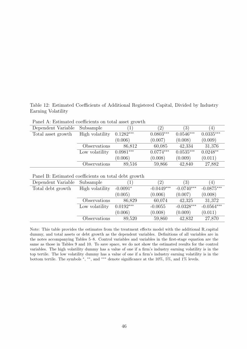
Table 12: Estimated Coefficients of Additional Registered Capital, Divided by IndustryEarning Volatility
Panel A: Estimated coefficients on total asset growthDependent Variable Subsample (1) (2) (3) (4)Total asset growth High volatility 0.1282∗∗∗ 0.0803∗∗∗ 0.0546∗∗∗ 0.0335∗∗∗
(0.006) (0.007) (0.008) (0.009)Observations 86,812 60,085 42,334 31,376
Low volatility 0.0981∗∗∗ 0.0774∗∗∗ 0.0535∗∗∗ 0.0248∗∗
(0.006) (0.008) (0.009) (0.011)Observations 89,516 59,866 42,840 27,882
Panel B: Estimated coefficients on total debt growthDependent Variable Subsample (1) (2) (3) (4)Total debt growth High volatility -0.0091∗ -0.0449∗∗∗ -0.0740∗∗∗ -0.0875∗∗∗
(0.005) (0.006) (0.007) (0.008)Observations 86,829 60,074 42,325 31,372
Low volatility 0.0192∗∗∗ -0.0055 -0.0328∗∗∗ -0.0564∗∗∗
(0.006) (0.008) (0.009) (0.011)Observations 89,520 59,860 42,832 27,870
Note: This table provides the estimates from the treatment effects model with the additional R capitaldummy, and total assets or debt growth as the dependent variables. Definitions of all variables are inthe notes accompanying Tables 5–8. Control variables and variables in the first-stage equation are thesame as those in Tables 9 and 10. To save space, we do not show the estimated results for the controlvariables. The high volatility dummy has a value of one if a firm’s industry earning volatility is in thetop tertile. The low volatility dummy has a value of one if a firm’s industry earning volatility is in thebottom tertile. The symbols ∗, ∗∗, and ∗∗∗ denote significance at the 10%, 5%, and 1% levels.
46
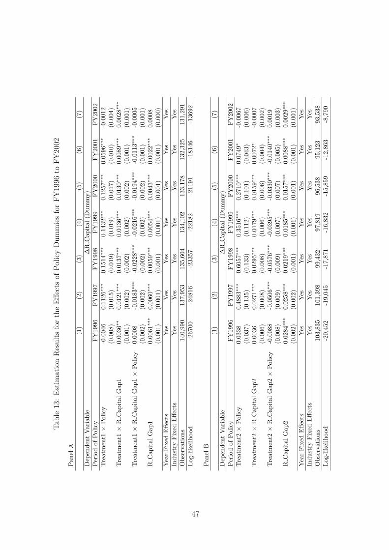
Tab
le13
:E
stim
atio
nR
esult
sfo
rth
eE
ffec
tsof
Pol
icy
Dum
mie
sfo
rFY
1996
toFY
2002
Pan
elA
(1)
(2)
(3)
(4)
(5)
(6)
(7)
Dep
ende
ntV
aria
ble
∆R
Cap
ital
(Dum
my)
Per
iod
ofPol
icy
FY
1996
FY
1997
FY
1998
FY
1999
FY
2000
FY
2001
FY
2002
Tre
atm
ent1
×Pol
icy
-0.0
046
0.11
26∗∗
∗0.
1514
∗∗∗
0.14
32∗∗
∗0.
1257
∗∗∗
0.05
96∗∗
∗-0
.001
2(0
.008
)(0
.015
)(0
.019
)(0
.019
)(0
.017
)(0
.010
)(0
.004
)Tre
atm
ent1
×R
Cap
ital
Gap
10.
0036
∗∗0.
0121
∗∗∗
0.01
37∗∗
∗0.
0136
∗∗∗
0.01
30∗∗
∗0.
0089
∗∗∗
0.00
28∗∗
∗
(0.0
01)
(0.0
02)
(0.0
02)
(0.0
02)
(0.0
02)
(0.0
01)
(0.0
01)
Tre
atm
ent1
×R
Cap
ital
Gap
1×
Pol
icy
0.00
08-0
.018
3∗∗∗
-0.0
228∗
∗∗-0
.021
6∗∗∗
-0.0
194∗
∗∗-0
.011
3∗∗∗
-0.0
005
(0.0
02)
(0.0
02)
(0.0
02)
(0.0
02)
(0.0
02)
(0.0
01)
(0.0
01)
RC
apit
alG
ap1
0.00
61∗∗
∗0.
0060
∗∗∗
0.00
59∗∗
∗0.
0054
∗∗∗
0.00
43∗∗
∗0.
0022
∗∗∗
0.00
08(0
.001
)(0
.001
)(0
.001
)(0
.001
)(0
.001
)(0
.001
)(0
.000
)Y
ear
Fix
edE
ffect
sY
esY
esY
esY
esY
esY
esY
esIn
dust
ryFix
edE
ffect
sY
esY
esY
esY
esY
esY
esY
esO
bser
vati
ons
140,
990
137,
953
135,
604
134,
102
133,
178
132,
325
131,
291
Log
-lik
elih
ood
-267
00-2
4816
-233
57-2
2182
-211
91-1
8146
-136
92
Pan
elB
(1)
(2)
(3)
(4)
(5)
(6)
(7)
Dep
ende
ntV
aria
ble
∆R
Cap
ital
(Dum
my)
Per
iod
ofPol
icy
FY
1996
FY
1997
FY
1998
FY
1999
FY
2000
FY
2001
FY
2002
Tre
atm
ent2
×Pol
icy
0.03
380.
4883
∗∗∗
0.60
57∗∗
∗0.
3516
∗∗∗
0.27
10∗∗
∗0.
0749
∗-0
.006
7(0
.037
)(0
.135
)(0
.133
)(0
.112
)(0
.101
)(0
.043
)(0
.006
)Tre
atm
ent2
×R
Cap
ital
Gap
20.
0036
0.02
71∗∗
∗0.
0295
∗∗∗
0.01
79∗∗
∗0.
0159
∗∗∗
0.00
72∗
-0.0
007
(0.0
06)
(0.0
08)
(0.0
08)
(0.0
06)
(0.0
06)
(0.0
04)
(0.0
02)
Tre
atm
ent2
×R
Cap
ital
Gap
2×
Pol
icy
-0.0
088
-0.0
506∗
∗∗-0
.057
6∗∗∗
-0.0
395∗
∗∗-0
.033
0∗∗∗
-0.0
140∗
∗∗0.
0019
(0.0
08)
(0.0
09)
(0.0
09)
(0.0
07)
(0.0
07)
(0.0
05)
(0.0
03)
RC
apit
alG
ap2
0.02
84∗∗
∗0.
0258
∗∗∗
0.02
19∗∗
∗0.
0185
∗∗∗
0.01
57∗∗
∗0.
0088
∗∗∗
0.00
29∗∗
∗
(0.0
02)
(0.0
02)
(0.0
01)
(0.0
01)
(0.0
01)
(0.0
01)
(0.0
01)
Yea
rFix
edE
ffect
sY
esY
esY
esY
esY
esY
esY
esIn
dust
ryFix
edE
ffect
sY
esY
esY
esY
esY
esY
esY
esO
bser
vati
ons
103,
835
101,
398
99,4
3297
,819
96,5
3895
,123
93,5
38Log
-lik
elih
ood
-20,
452
-19,
045
-17,
871
-16,
832
-15,
859
-12,
863
-8,7
90
47

Pan
elC
(1)
(2)
(3)
(4)
(5)
(6)
(7)
Dep
ende
ntV
aria
ble
∆R
Cap
ital
(Dum
my)
Per
iod
ofPol
icy
FY
1996
FY
1997
FY
1998
FY
1999
FY
2000
FY
2001
FY
2002
Tre
atm
ent3
×Pol
icy
-0.0
108∗
∗∗0.
0441
∗∗∗
0.06
63∗∗
∗0.
0675
∗∗∗
0.06
84∗∗
∗0.
0416
∗∗∗
0.00
62∗∗
(0.0
04)
(0.0
09)
(0.0
11)
(0.0
11)
(0.0
11)
(0.0
08)
(0.0
03)
Tre
atm
ent3
×R
Cap
ital
Gap
3-0
.001
70.
0065
∗∗∗
0.00
58∗∗
∗0.
0054
∗∗∗
0.00
60∗∗
∗0.
0048
∗∗∗
0.00
08(0
.002
)(0
.001
)(0
.001
)(0
.001
)(0
.001
)(0
.001
)(0
.001
)Tre
atm
ent3
×R
Cap
ital
Gap
3×
Pol
icy
0.00
68∗∗
∗-0
.018
7∗∗∗
-0.0
219∗
∗∗-0
.021
9∗∗∗
-0.0
207∗
∗∗-0
.013
6∗∗∗
-0.0
021∗
∗
(0.0
02)
(0.0
02)
(0.0
02)
(0.0
02)
(0.0
02)
(0.0
01)
(0.0
01)
RC
apit
alG
ap3
0.08
28∗∗
∗0.
0746
∗∗∗
0.06
61∗∗
∗0.
0589
∗∗∗
0.05
30∗∗
∗0.
0396
∗∗∗
0.02
48∗∗
∗
(0.0
02)
(0.0
02)
(0.0
02)
(0.0
02)
(0.0
01)
(0.0
01)
(0.0
01)
Yea
rFix
edE
ffect
sY
esY
esY
esY
esY
esY
esY
esIn
dust
ryFix
edE
ffect
sY
esY
esY
esY
esY
esY
esY
esO
bser
vati
ons
72,6
8071
,357
70,4
3369
,401
69,0
0968
,118
66,6
66Log
-lik
elih
ood
-11,
832
-10,
832
-10,
097
-9,5
66-9
,118
-7,1
95-4
,621
Not
e:T
his
tabl
epr
esen
tses
tim
ates
ofpr
obit
and
tobi
tre
gres
sion
sw
ith
the
addi
tion
alR
capi
tal
dum
my
asde
pend
ent
vari
able
s.T
head
diti
onal
Rca
pita
ldum
my
(sho
wn
as“D
umm
y”in
the
tabl
e)is
adu
mm
yva
riab
leth
atha
sa
valu
eof
one
ifre
gist
ered
capi
tali
sla
rger
atth
een
dof
fisca
lyea
rt
than
atth
ebe
ginn
ing
offis
calye
art.
Defi
niti
ons
ofin
depe
nden
tva
riab
les
are
show
nin
the
note
toTab
les
5,6,
7,an
d8.
The
mar
gina
leff
ects
ofea
chva
riab
lear
esh
own
inth
ista
ble.
Est
imat
edro
bust
stan
dard
erro
rsar
esh
own
inpa
rent
hese
s.T
hesy
mbo
ls∗ ,
∗∗,an
d∗∗
∗de
note
sign
ifica
nce
atth
e10
%,5%
,an
d1%
leve
ls.
48