smip03 seminar on utilization of strong-motion data ... · department of conservation established a...
TRANSCRIPT
SMIP03
SMIP03 SEMINAR ON UTILIZATION OF STRONG-MOTION DATA
Oakland, California May 22, 2003
PROCEEDINGS
Sponsored by
California Strong Motion Instrumentation Program California Geological Survey
California Department of Conservation
Supported in Part by
California Seismic Safety Commission California Office of Emergency Services
CALIFORNIA GEOLOGICAL SURVEY
The California Strong Motion Instrumentation Program (CSMIP) is a program within the California Geological Survey (previously known as the Division of Mines and Geology) of the California Department of Conservation. It is advised by the Strong Motion Instrumentation Advisory Committee (SMIAC), a committee of the California Seismic Safety Commission. Major program funding is provided by an assessment on construction costs for building permits issued by cities and counties in California, with additional funding from the California Office of Emergency Services, the California Department of Transportation, the Office of Statewide Health Planning and Development and the California Department of Water Resources. In 1997, a joint project, TriNet, between CSMIP, Caltech and USGS at Pasadena was funded by the Federal Emergency Management Agency (FEMA) through the California Office of Emergency Services (OES). The goals of the project were to record and rapidly communicate ground shaking information in southern California, and to analyze the data for the improvement of seismic codes and standards. TriNet produced ShakeMaps of ground shaking, based on shaking recorded by stations in the network, within minutes following an earthquake. The ShakeMap identifies areas of greatest ground shaking for use by OES and other emergency response personnel in the event of a damaging earthquake. In July 2001, the California Office of Emergency Services began funding for the California Integrated Seismic Network (CISN), a newly formed consortium of institutions engaged in statewide earthquake monitoring that grew out of TriNet, and includes CGS, USGS, Caltech and UC Berkeley. The CISN will improve seismic instrumentation and provide statewide ground shaking intensity maps. It will also distribute and archive strong-motion records of engineering interest and seismological data for all recorded earthquakes, and provide training for users. DISCLAIMER Neither the sponsoring nor supporting agencies assume responsibility for the accuracy of the information presented in this report or for the opinions expressed herein. The material presented in this publication should not be used or relied upon for any specific application without competent examination and verification of its accuracy, suitability, and applicability by qualified professionals. Users of information from this publication assume all liability arising from such use.
SMIP03
SMIP03 SEMINAR ON UTILIZATION OF STRONG-MOTION DATA
Oakland, California May 22, 2003
PROCEEDINGS
Edited by
Moh Huang
Sponsored by
California Strong Motion Instrumentation Program California Geological Survey
California Department of Conservation
Supported in Part by
California Seismic Safety Commission California Office of Emergency Services


SMIP03 Seminar Proceedings
i
PREFACE The California Strong Motion Instrumentation Program (CSMIP) in the California Geological Survey (previously known as the Division of Mines and Geology) of the California Department of Conservation established a Data Interpretation Project in 1989. Each year the CSMIP funds several data interpretation contracts for the analysis and utilization of strong-motion data. The primary objectives of the Data Interpretation Project are to further the understanding of strong ground shaking and the response of structures, and to increase the utilization of strong-motion data in improving post-earthquake response, seismic code provisions and design practices. As part of the Data Interpretation Project, CSMIP holds annual seminars to transfer recent research findings on strong-motion data to practicing seismic design professionals, earth scientists and post-earthquake response personnel. The purpose of the annual seminar is to provide information that will be useful immediately in seismic design practice and post-earthquake response, and in the longer term, in the improvement of seismic design codes and practices. The SMIP03 Seminar is the fourteenth in this series of annual seminars.
The SMIP03 Seminar is divided into four sessions. Session I includes two presentations on ground motion topics. Session II will focus on post-earthquake response and includes updates on ShakeMap and the CISN Engineering Data Center, and the final report on the ATC-54 Guidelines for Using Strong-Motion Data and ShakeMap in Post-Earthquake Response. There will also be an update on HAZUS loss estimation using ShakeMap. Session III will include two presentations on lifeline structures. Session IV will include two presentations on buildings. The Seminar will end with a field trip to the Oakland City Hall. Before the field trip, we have invited Mason Walters to discuss the design approach and new structural system for strengthening the City Hall. This will be followed with a presentation on the strong-motion instrumentation and recorded strong-motion data from the City Hall. The seminar will include presentations by investigators of seven CMIP-funded projects. Four projects have been completed and their final reports will be available this year. The other three projects are scheduled to be completed by the end of 2003, so the investigators can only present preliminary or interim results. The final results will be presented at the next year’s seminar (SMIP04). Moh J. Huang Data Interpretation Project Manager

SMIP03 Seminar Proceedings
ii
Members of the Strong Motion Instrumentation Advisory Committee
Main Committee
Chris Poland, Chair, Degenkolb Engineers Bruce Bolt, UC Berkeley Anil Chopra, UC Berkeley Bruce Clark, Seismic Safety Commission, Leighton & Associates C. Allin Cornell, Stanford University Wilfred Iwan, California Institute of Technology Jerve Jones, Peck/Jones Construction Corp. Vern Persson, DWR Div. of Safety of Dams (retired) Daniel Shapiro, Seismic Safety Commission, SOHA Engineers Ray Zelinski, Caltrans Edward Bortugno (ex-officio), Office of Emergency Services Richard McCarthy (ex-officio), Seismic Safety Commission
Groud Response Subcommittee Bruce Bolt, Chair, UC Berkeley Brian Chiou, Caltrans Marshall Lew, Law/Crandall Geoffrey Martin, Univ. of Southern California Maurice Power, Geomatrix Consultants
Buildings Subcommittee Chris Poland, Chair, Degenkolb Engineers Kenneth Honda, URS Corporation Donald Jephcott, Structural Engineer Jerve Jones, Peck/Jones Consttuction Corp. Jack Meehan, Structural Engineer Farzad Naeim, John A. Martin & Associates John Robb, Structural Engineer Zan Turner, City and County of San Francisco Chia-Ming Uang, UC San Diego
Lifelines Subcommittee Vern Persson, Chair, DWR Div. of Safety of Dams (retired) Martin Eskijian, California State Lands Commission David Gutierrez, DWR Div. of Safety of Dams LeVal Lund, Civil Engineer Edward Matsuda, BART Ron Tognazzini, Los Angeles Dept. of Water and Power Ray Zelinski, Caltrans
Data Utilization Subcommittee Wilfred Iwan, Chair, California Institute of Technology Representatives from each Subcommittee
SMIP03 Seminar Proceedings
iii
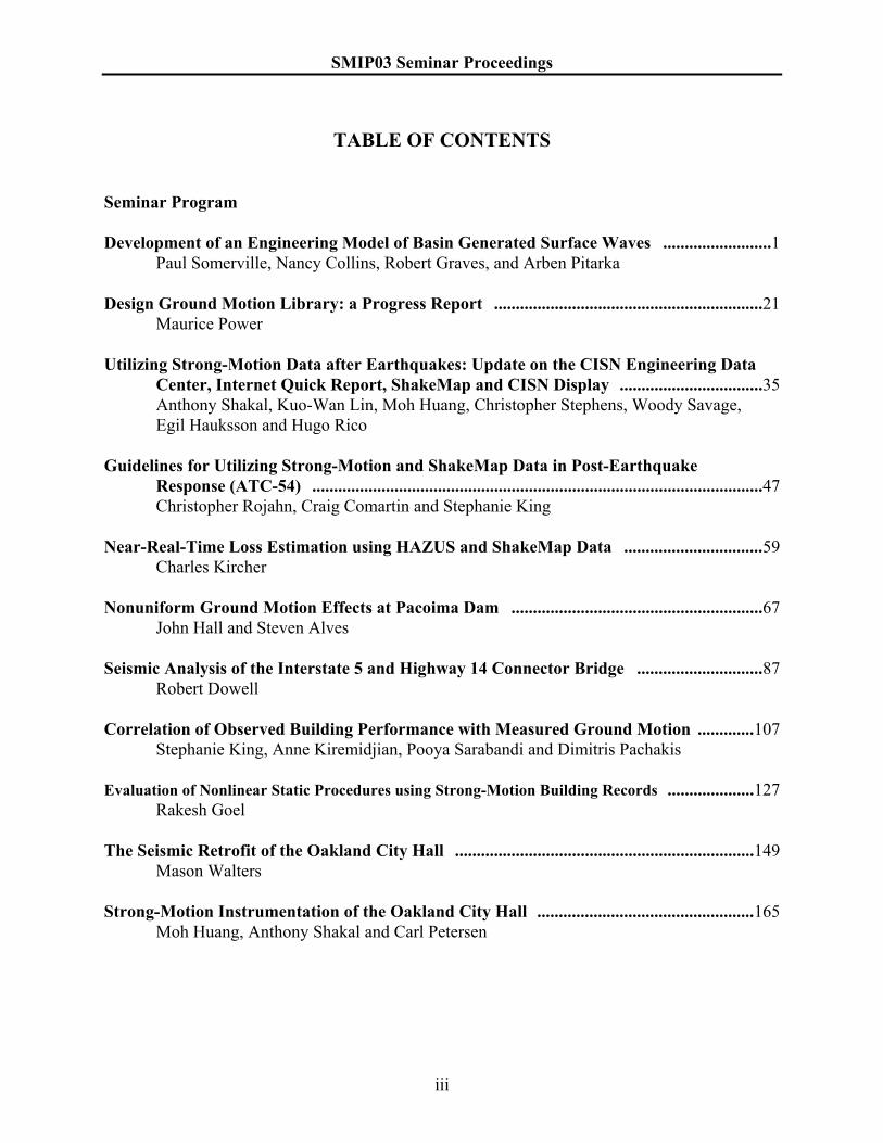
TABLE OF CONTENTS
Seminar Program Development of an Engineering Model of Basin Generated Surface Waves .........................1 Paul Somerville, Nancy Collins, Robert Graves, and Arben Pitarka Design Ground Motion Library: a Progress Report ..............................................................21 Maurice Power Utilizing Strong-Motion Data after Earthquakes: Update on the CISN Engineering Data Center, Internet Quick Report, ShakeMap and CISN Display .................................35 Anthony Shakal, Kuo-Wan Lin, Moh Huang, Christopher Stephens, Woody Savage, Egil Hauksson and Hugo Rico Guidelines for Utilizing Strong-Motion and ShakeMap Data in Post-Earthquake Response (ATC-54) ........................................................................................................47 Christopher Rojahn, Craig Comartin and Stephanie King Near-Real-Time Loss Estimation using HAZUS and ShakeMap Data ................................59 Charles Kircher Nonuniform Ground Motion Effects at Pacoima Dam ..........................................................67 John Hall and Steven Alves Seismic Analysis of the Interstate 5 and Highway 14 Connector Bridge .............................87 Robert Dowell Correlation of Observed Building Performance with Measured Ground Motion .............107 Stephanie King, Anne Kiremidjian, Pooya Sarabandi and Dimitris Pachakis Evaluation of Nonlinear Static Procedures using Strong-Motion Building Records ....................127 Rakesh Goel The Seismic Retrofit of the Oakland City Hall .....................................................................149 Mason Walters Strong-Motion Instrumentation of the Oakland City Hall ..................................................165 Moh Huang, Anthony Shakal and Carl Petersen

SMIP03 Seminar Proceedings
iv

SMIP03 Seminar Proceedings
v
SMIP03 SEMINAR ON
UTILIZATION OF STRONG-MOTION DATA Oakland Marriott City Center, Oakland, California May 22, 2003
FINAL PROGRAM 8:00 am REGISTRATION
9:00 am WELCOMING REMARKS Wilfred Iwan, Strong Motion Instrumentation Advisory Committee (SMIAC) James Davis, State Geologist, California Geological Survey
INTRODUCTORY REMARKS Anthony Shakal and Moh Huang, Strong Motion Instrumentation Program
Moderator: Bruce Bolt, UC Berkeley, SMIAC 9:15 am Development of an Engineering Model of Basin Generated Surface Waves Paul Somerville, Robert Graves, and Arben Pitarka, URS Group, Inc.
9:40 am Design Ground Motion Library: a Progress Report Maurice Power, Geomatrix Consultants
10:05 am Questions and Answers for Session I 10:15 am Break
Moderator: Wilfred Iwan, Caltech, SMIAC 10:35 am Utilizing Strong-Motion Data after Earthquakes: Update on the CISN
Engineering Data Center, Internet Quick Report, ShakeMap and CISN Display Anthony Shakal, Kuo-Wan Lin and Moh Huang, CSMIP, Woody Savage and Chris
Stephens, USGS/NSMP, Egill Hauksson and Hugo Rico, Caltech
10:50 am Guidelines for Utilizing Strong-Motion and ShakeMap Data in Post-Earthquake Response (ATC-54)
Christopher Rojahn, Applied Technology Council; Craig Comartin, Comartin-Reis; and Stephanie King, Hart-Weidlinger
11:15 am Near-Real-Time Loss Estimation Using HAZUS and Shakemap Data Charles Kircher, Kircher & Associates
11:35 am Questions and Answers for Session II
SESSION I
SESSION II

SMIP03 Seminar Proceedings
vi
11:45 am LUNCH
Moderator: Vern Persson, SMIAC 12:45 pm Nonuniform Ground Motion Effects at Pacoima Dam John Hall and Steven Alves, Caltech
1:10 pm Seismic Analysis of the Interstate 5 and Highway 14 Connector Bridge Robert Dowell, Dowell-Holombo Engineering, Inc.
1:35 pm Questions and Answers for Session III 1:45 pm Break
Moderator: Farzad Naeim, John A. Martin and Associates, SMIAC
2:00 pm Correlation of Observed Building Performance with Measured Ground Motion Stephanie King, Hart-Weidlinger; Anne Kiremidjian, Pooya Sarabandi and Dimitris
Pachakis, Stanford University
2:25 pm Evaluation of Nonlinear Static Procedures Using Strong-Motion Building Records
Rakesh Goel, California Polytechnic State University, San Luis Obispo 2:50 am Questions and Answers for Session IV
3:00 pm Field Trip Introduction Seismic Retrofit of the Oakland City Hall Mason Walters, Forell/Elsesser Engineers
3:20 pm Field Trip Introduction Strong-Motion Instrumentation of the Oakland City Hall Moh Huang, Anthony Shakal and Carl Petersen, CSMIP
3:30 pm Field Trip to Oakland City Hall
SESSION III
SESSION IV
SMIP03 Seminar Proceedings
1
DEVELOPMENT OF AN ENGINEERING MODEL OF BASIN GENERATED SURFACE WAVES
Paul G. Somerville, Nancy Collins, Robert Graves, and Arben Pitarka
URS Group, Inc., Pasadena, CA
Abstract
We have developed a modification to the ground motion model of Abrahamson et al. (1997) that takes into account the effects of basin generated surface waves. The main feature of our model is that for response spectral accelerations at periods of 4 and 5 seconds, the Abrahamson and Silva (1997) model for soil sites should be scaled by a factor of 1.65 in order to represent the ground motions on soil sites located within sedimentary basins. Our finding that no scaling of the Abrahamson and Silva (1997) model is required for periods shorter than 4 seconds reflects the fact that most of the deep soil recordings on which that model is based come from sedimentary basins. The fact that our first order model does not have a dependence on distance to the basin edge or the depth of the basin makes it easily applicable in ground motion calculations, especially those for probabilistic seismic hazard analyses, which typically involve the calculation of ground motions from many different scenario earthquakes occurring on a variety of faults surrounding the site. We have identified many second order basin effects that are not quantified in our first order model of basin effects.
Introduction
Many urban regions are situated on deep sediment-filled basins. A basin consists of alluvial
deposits and sedimentary rocks that are geologically younger and have lower seismic wave velocities than the underlying rocks upon which they have been deposited. Basins have thickness ranging from a hundred meters to over ten kilometers. It is widely recognized that sedimentary basins have a strong influence on strong ground motions, especially at periods longer than about one second. However, most empirical ground motion models do not explicitly account for these effects.
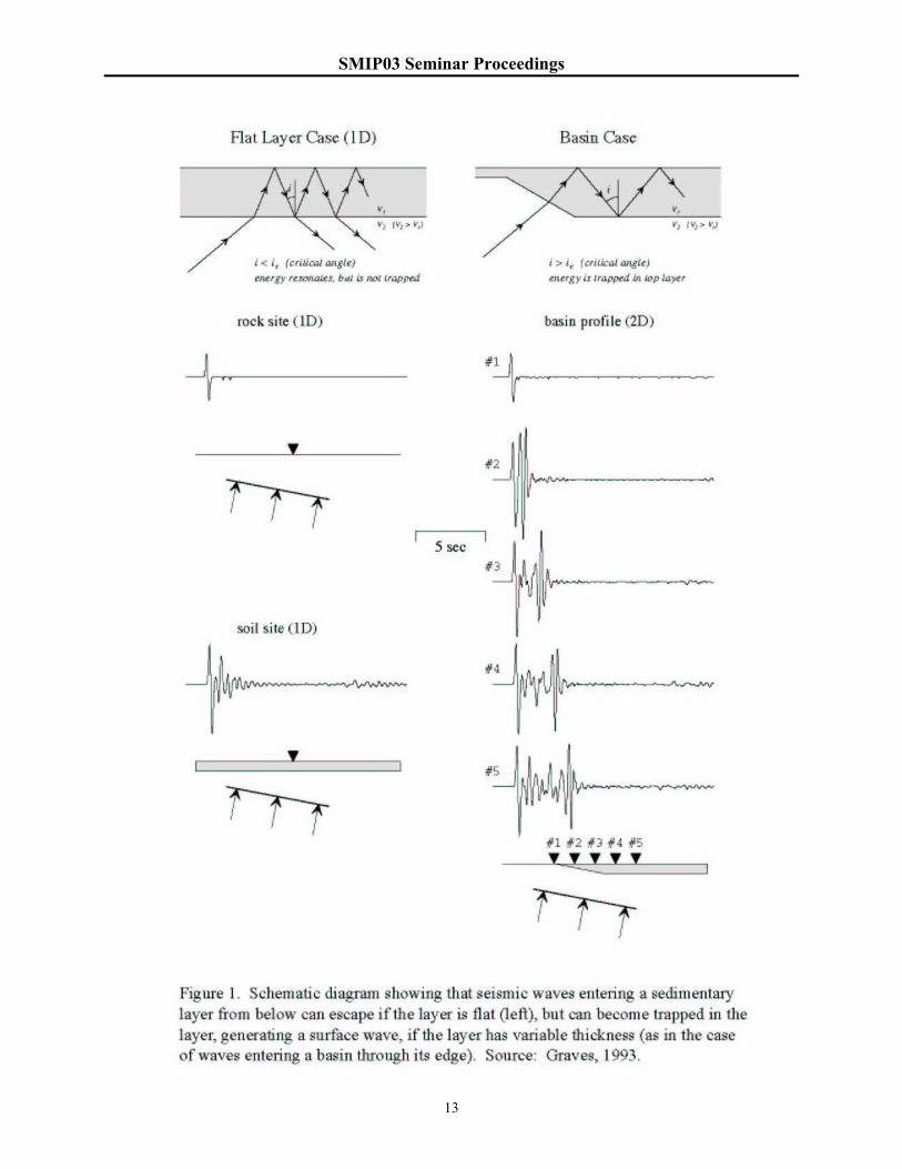
Current building code criteria including the 1997 UBC (ICBO, 1997) and 2000 NEHRP
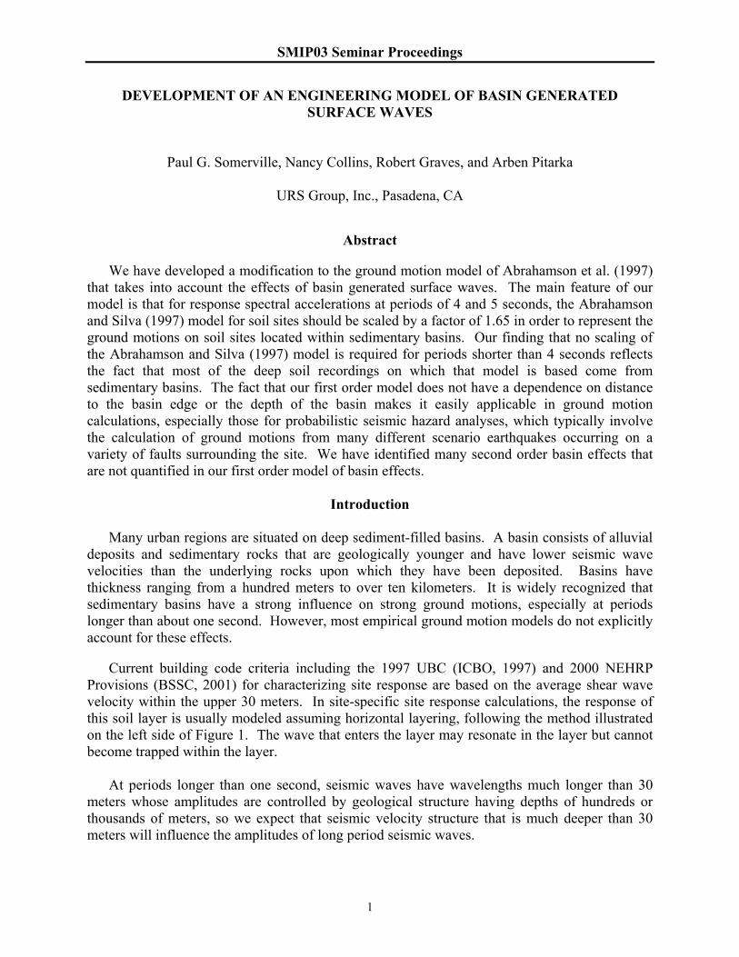
Provisions (BSSC, 2001) for characterizing site response are based on the average shear wave velocity within the upper 30 meters. In site-specific site response calculations, the response of this soil layer is usually modeled assuming horizontal layering, following the method illustrated on the left side of Figure 1. The wave that enters the layer may resonate in the layer but cannot become trapped within the layer.
At periods longer than one second, seismic waves have wavelengths much longer than 30
meters whose amplitudes are controlled by geological structure having depths of hundreds or thousands of meters, so we expect that seismic velocity structure that is much deeper than 30 meters will influence the amplitudes of long period seismic waves.

SMIP03 Seminar Proceedings
2
In most cases, such as in sedimentary basins, this deeper geological structure is not horizontally layered. If the wave is propagating in the direction in which the basin is thickening and enters the basin through its edge, it can become trapped within the basin if post-critical incidence angles develop. The resulting total internal reflection at the base of the layer is illustrated at the top right of Figure 1.
In the lower part of Figure 1, simple calculations of the basin response are compared with
those for the simple horizontal layered model. In each case, a plane wave is incident at an inclined angle from below. The left side of the figure shows the amplification due to impedance contrast effects that occurs on a flat soil layer overlying rock (bottom) relative to the rock response (top). A similar amplification effect is shown for the basin case on the right side of the figure. However, in addition to this amplification, the body wave entering the edge of the basin becomes trapped, generating a surface wave that propagates across the basin.
The development of basin generated surface waves is illustrated in the strong motion
recordings of many earthquakes. As an example, the top of Figure 2 shows the location of the fault plane of the 1992 Petrolia earthquake, and the locations of strong motion recording stations in and near the Eel River basin. The direct S wave arrival is shown by the dashed lines in the profiles of filtered velocity waveforms in the bottom of Figure 2. The development of surface waves propagating across the basin is clearly evident in the later arriving phase, indicated by the solid lines. The Eel River basin is about 3 km thick at its deepest point. The surface waves are not present in the recording at station “bunk,” which lies outside the basin. The influence of basin structure on recorded ground motions is well explained by basic seismological theory (e.g. Vidale and Helmberger, 1988; Wald and Graves, 1998), and efficient computational procedures have been developed for the modeling of seismic wave propagation in basins (e.g. Graves, 1996; Pitarka, 1999).
Ground Motion Models that Address Basin Structure
Most current empirical ground motion attenuation relations do not distinguish between sites
located on shallow alluvium and those located on sedimentary basins. Consequently, these relations may tend to underestimate the ground motions recorded in basins and overestimate those recorded outside basins. However, the influence of basin effects on the amplitudes of strong ground motions has been recognized and incorporated in several ground motion models. These models incorporate basin effects through simplified representations of the basement structure, such as the depth to basement rock beneath the recording site, and the distance from the recording site to the edge of the basin. The depth to basement rock was used as a parameter in the empirical ground motion models of Trifunac and Lee (1979) and Campbell (1997). Lee and Anderson (2000), Field (2002), and Hruby and Beresnev (2002) found that peak accelerations increased with depth to basement in the Los Angeles basin. In the most detailed model for basin effects that has been developed to date (Joyner, 2000), the effect of the basin depends on the distance of the site from the basin edge.
The Joyner (2000) model incorporates differences in ground motion amplitude between the
basin edge parallel and basin edge normal components. This model is based on the expectation that there is lateral refraction of surface waves at the basin edge. Alternative models could be
SMIP03 Seminar Proceedings
3
based on the radial and tangential components, or on the average horizontal component. Accordingly, we tested the Joyner (2000) assumption against recorded data as a preliminary step before proceeding with our full analysis of basin effects. We used recordings of the 1999 Hector Mine earthquake in the San Bernardino basin (Wald and Graves, 2003) to analyze the polarization of basin surface waves. These recordings provide clear evidence of lateral refraction of surface waves at the basin edge, which causes the basin waves to be polarized predominantly in the directions parallel to and normal to the edge of the basin, with Love waves predominating on the parallel direction and Rayleigh waves predominating on the normal direction. This is consistent with the assumption made by Joyner (2000). Our analysis also indicates that there can be clear differences in the amplitudes of the basin edge parallel and basin edge normal components. These amplitudes are affected by the relative strength of the incoming waves, which depends on focal mechanism and other factors.
We also used the San Bernardino basin recordings of the 1999 Hector Mine earthquake to
analyze the effect of basin depth and distance from basin edge, which are parameters in the Joyner (2000) model, on basin wave amplitudes. The peak velocity increases markedly when the waves enter the San Bernardino basin, and grows in amplitude with increasing distance from the basin edge, even though the distance from the source is increasing. This is due to the trapping of body waves that enter the basin, generating surface waves. There is a clear correlation of peak velocity with basin depth. When depth increases away from the basin edge (i.e. when basin depth and basin edge distance are correlated), this can cause ground motion amplitudes to increase away from the basin edge, and so the basin depth and distance from basin edge do affect basin wave amplitudes, as in the Joyner (2000) model. However, we will show that in most basins this correlation does not hold, apparently due to complexity in basin geometry.
Selection of Strong Motion Recordings for Analysis
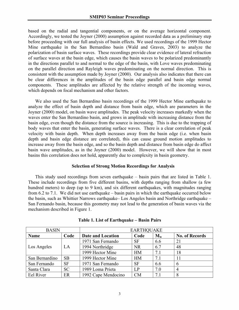
This study used recordings from seven earthquake – basin pairs that are listed in Table 1.
These include recordings from five different basins, with depths ranging from shallow (a few hundred meters) to deep (up to 9 km), and six different earthquakes, with magnitudes ranging from 6.2 to 7.1. We did not use earthquake – basin pairs in which the earthquake occurred below the basin, such as Whittier Narrows earthquake– Los Angeles basin and Northridge earthquake – San Fernando basin, because this geometry may not lead to the generation of basin waves via the mechanism described in Figure 1.
Table 1. List of Earthquake – Basin Pairs
BASIN EARTHQUAKE
Name Code Date and Location Code Mw No. of Records 1971 San Fernando SF 6.6 21 1994 Northridge NR 6.7 48
Los Angeles
LA
1999 Hector Mine HM 7.1 18 San Bernardino SB 1999 Hector Mine HM 7.1 11 San Fernando SF 1971 San Fernando SF 6.6 6 Santa Clara SC 1989 Loma Prieta LP 7.0 4 Eel River ER 1992 Cape Mendocino CM 7.1 8
SMIP03 Seminar Proceedings
4
Development of a Model For Basin Wave Amplitudes Our approach to developing the ground motion model is to calculate residuals between the
recorded ground motions and the predictions of the Abrahamson and Silva (1997) model, and seek correlations between these residuals and basin parameters such as the depth of the basin beneath the recording site, and the distance of the recording site from the edge of the basin. These residuals were first calculated for individual earthquake – basin pairs, and the average values within distance and depth bins were calculated to facilitate the identification of trends of the data. These residuals were then averaged across earthquake - basin pairs to facilitate the identification of general trends.
In Figures 3 and 4, we show residuals averaged over these earthquake – basin pairs for
response spectral acceleration having periods of 5, 4, 3, 2, 1.5 and 1 second. The residuals for depth to basement for individual basin – earthquake pairs are quite variable. The Hector Mine earthquake – San Bernardino basin data show the ideal behavior that was described above, in which the peak amplitude increases systematically with increasing depth to basement. Most other earthquake – basin pairs do not show this ideal behavior. The Los Angeles basin residuals from the San Fernando and Hector Mine earthquakes are uniformly high for periods of 4 and 5 seconds, while the residuals for the Northridge earthquake are uniformly low for periods of 3 seconds and longer, especially on the basin edge parallel component. We attribute these systematic differences to differences in closest distance and earthquake source depth, as described further below.
The aggregated residuals for depth to basement, shown in Figure 3, are systematically
positive for periods of 4 and 5 seconds, especially on the basin edge parallel component, indicating that the model underpredicts the data. The positive residuals in this period range do not show a systematic dependence on basement depth. The residuals, averaged over the depth range of 0 – 4 km, have an average value of 0.5 natural log units, corresponding to a factor of 1.65. For periods of 2, 1.5 and 1 seconds, the residuals are slightly negative, indicating that the model slightly overpredicts the data.
The residuals for distance from basin edge have patterns that are similar to those depth to
basement described above. The residuals for individual basin – earthquake pairs are quite variable. The Hector Mine earthquake – San Bernardino basin data show ideal behavior, in which the peak amplitude increases systematically with increasing distance from the basin edge. Most other earthquake – basin pairs do not show this ideal behavior. The Los Angeles basin residuals from the San Fernando and Hector Mine earthquakes are uniformly high for periods of 4 and 5 seconds, while the residuals for the Northridge earthquake are uniformly low for periods of 3 seconds and longer, especially on the basin edge parallel component. We attribute these systematic differences to differences in closest distance and earthquake source depth, as described further below.
The aggregated residuals for distance to basin edge, shown in Figure 4, are systematically
positive for periods of 4 and 5 seconds, especially on the basin edge parallel component, indicating that the model underpredicts the data. The residuals for the basin edge parallel component show little dependence on distance from the basin edge, while the residuals for the

SMIP03 Seminar Proceedings
5
basin edge normal component are small at close distances but grow larger for greater distances. This difference in behavior is described in more detail below. To first order, we model the residuals in this period range as not having a systematic dependence on distance to basin edge, which is most nearly true of the basin edge parallel component. The residuals, averaged over the distance to basin edge range of 0 – 40 km, have an average value of 0.5 natural log units, corresponding to a factor of 1.65. For periods of 2, 1.5 and 1 seconds, the residuals are slightly negative, indicating that the model slightly overpredicts the data.
The residuals for some earthquake – basin pairs are systematically high, while those for
others are systematically low. For example, the Los Angeles basin residuals for the San Fernando and Hector Mine earthquakes are uniformly high for periods of 4 and 5 seconds, while the residuals for the Northridge earthquake are uniformly low for periods of 3 seconds and longer. In Table 2, we list these earthquake – basin pairs, indicating whether the residuals are systematically high (+), neutral (o) or low (–), and also indicating whether the earthquake is shallow (significant amount of slip shallower than 5 km) or deep, and whether the earthquake is close (closest distance from most recording stations less than 20 km) or distant.
Table 2. Correlation of Residuals with Earthquake Source Depth and Distance
Earthquake Source Depth
Basin Distance Observed residuals
Predicted residuals
San Fernando shallow San Fernando close o o Los Angeles distant + + Northridge deep Los Angeles distant – – Hector Mine shallow San Bernardino distant + + Los Angeles distant + + Loma Prieta deep Gilroy close – – Cape Mendocino deep Eel River close o –
All of the instances of positive residuals in Table 2 are associated with shallow faulting of
distant earthquakes. Shallow faulting on distant sources is associated with shallower incidence (larger incidence angle) of waves entering the basin (Figure 1), making it more likely that postcritical angles will develop inside the basin. We postulate that this is the cause of the positive residuals for shallow distant earthquakes.
In contrast, all of the instances of negative residuals in Table 2 are associated with deep
faulting on nearby sources. Deep faulting on nearby sources is associated with steeper incidence (smaller incidence angle) of waves entering the basin (Figure 1), making it less likely that postcritical angles will develop inside the basin. We postulate that this is the cause of the negative residuals for deep nearby earthquakes. We applied this hypothesis related to incidence angle to predict the nature of the residuals that are expected in each earthquake – basin pair in Table 2, and show the prediction next to the observed residuals. In each case, the hypothesis is consistent with the observed residual.

SMIP03 Seminar Proceedings
6
We can test the separate influences of distance and depth in the following way. The shallow faulting San Fernando earthquake was recorded in both the San Fernando basin and the Los Angeles basin. The Los Angeles basin residuals are positive, while the San Fernando basin residuals are neutral. We attribute this to the shallower angle of incidence for waves entering the Los Angeles basin than the San Fernando basin, due to the larger distance of the San Fernando earthquake.
Ground motions from both the shallow San Fernando earthquake and the deep Northridge
earthquake were recorded in the Los Angeles basin, at comparable distances. The San Fernando earthquake residuals are positive, and the Northridge earthquake residuals are negative. We attribute this to the shallower angle of incidence for waves entering the Los Angeles basin from the San Fernando earthquake compared with the Northridge earthquake, due to the shallower depth of the San Fernando earthquake.
Our hypothesis is consistent with the trend of increasingly positive residuals with increasing
distance, as measured in two ways. In Figure 5, the distance measure is the closest distance to the recording site, including both the segment of the path outside the basin and the segment of the path inside the basin. In Figure 6, the distance measure is the distance from the epicenter to the basin edge, including only the segment of the path outside the basin. For both distance measures, the residuals for periods of 4 and 5 seconds increase with increasing distance, consistent with our hypothesis that the incidence angle controls the likelihood that basin generated surface waves will become trapped, causing positive residuals.
Discussion of Results
Basin Adjustment Factors for the Abrahamson and Silva (1997) Model
To a first approximation, the ground motions recorded in basins are a factor of 1.65 stronger
for periods of 4 and 5 seconds than predicted by the Abrahamson and Silva (1997) ground motion model. At periods of 3 seconds and less, no adjustment factor is required; if anything, the ground motions at periods of 1, 1.5 and 2 seconds in this model overpredicts the data. We consider this result to be consistent with the composition of the strong motion data set from which the Abrahamson and Silva (1997) model is derived. Recent large earthquakes that have numerous recordings in basins, such as the 1992 Cape Mendocino, 1992 Landers, and 1994 Northridge earthquakes, are included in the model. The recordings are all from sites with more than 20 meters of soil over bedrock. These deep soil sites are likely to be influenced by surface waves, at least for periods of a few seconds, even if they are not located on deep basins, and so their ground motions on average are adequately predicted by the Abrahamson and Silva (1997) model. However, only those sites located on deep basins are likely to be influenced by basin waves having periods of 4 and 5 seconds, so these ground motions on average are underpredicted by the Abrahamson and Silva (1997) model. In this respect, our model is compatible with the model of Joyner (2000), in which the adjustment factors for the Abrahamson and Silva (1997) model are large only for periods of 4 and 5 seconds.

SMIP03 Seminar Proceedings
7
Averaged over all recordings of all earthquakes, the residuals do not have a strong dependence on distance from the basin edge and on the depth of the basin at the site. Accordingly, we consider that, to a first approximation, it is sufficient to apply the adjustment factors without consideration of these parameters. This considerably simplifies the application of the adjustment factors to the prediction of strong ground motion, compared with the Joyner (2000) model, especially in a probabilistic seismic hazard calculation that addresses a large number of earthquakes occurring at various locations around the basin site. However, there are trends in the residuals that pertain to particular conditions that could be addressed in the calculation of ground motions for specific earthquake scenarios. We address these conditions in the following paragraphs.
Correlation of Basin Wave Amplitude with Distance to Basin Edge and Basin Depth in
Simple Basins In simple basins, in which the basin thickens smoothly from the basin edge, there is a clear
increase of basin wave amplitude with increasing distance from the basin edge and with increasing basin depth, when the earthquake source is shallow. The San Bernardino Basin recordings of the 1999 Hector Mine earthquake provide a clear example of this behavior, which is consistent with simple 2D calculations of basin waves in a thickening basin. If a site is located in this kind of situation, the first order model described above will tend to underestimate the ground motions at distances larger than about 10 km from the basin edge.
Differences in Amplitude between Basin Edge Parallel and Normal Components
There are significant differences between the amplitudes of the horizontal component parallel
to and perpendicular to the basin edge. This is seen in the residuals for periods of 4 and 5 seconds as a function of distance shown in Figure 4. The residuals for the basin edge parallel component show little dependence on distance from the basin edge, while the residuals for the basin edge normal component are small at close distances but grow larger for greater distances. This behavior is consistent with that in the Joyner (2000) model. In his model, at close distances to the basin edge, the ground motion in the parallel direction is larger than in the perpendicular direction. However, the ground motion in the parallel direction attenuates more rapidly with distance from the basin edge than does the perpendicular component, so at large distances the perpendicular component is larger in his model, with a crossover at about 60 km that varies with period. Our residuals indicate that the basin edge normal component does not grow larger than the basin edge parallel component, contrary to the Joyner (2000) model.
We expect the relative amplitudes of the basin edge parallel and basin edge normal
components to be affected by the relative strength of the incoming waves, which depends on focal mechanism and other factors, and on refraction effects. Given the expected complexity of these effects, the observed pattern of relative amplitudes is surprisingly simple. Where there are differences between the two components, which is usually at periods of 3 seconds or longer, the basin edge parallel component is consistently stronger than the basin edge normal component. This is true of individual earthquakes, regardless of focal mechanism, as well as of the data set as a whole.
SMIP03 Seminar Proceedings
8
This result may be attributed to the following cause. For waves with normal incidence on the basin edge, the edge parallel component consists of SH waves that become trapped in the basin as Love waves. These waves are not subject to mode conversion. In contrast, SV waves polarized in the basin edge normal direction would be subject to mode conversion from S to P waves, reducing the strength of the S waves that are transmitted into the basin. This may explain the observation that basin waves on the basin edge parallel component are systematically higher than those on the basin edge normal component.
The residuals between recorded basin ground motions and those computed from the
Abrahamson and Silva (1997) model are largest and most consistent for the basin edge parallel component. Positive residuals are also present in the vertical component and to a lesser extent in the basin edge normal component. We recommend that, for simplicity and for conservatism, the distance-independent adjustment factor derived from the basin edge parallel component be applied to all three components of motion.
Dependence of Basin Wave Amplitude on Earthquake Depth
Shallow crustal earthquakes generate significantly stronger basin waves (and larger positive
residuals from the Abrahamson and Silva, 1997 model) than do deeper crustal earthquakes. Examples of shallow crustal earthquakes include the 1971 San Fernando, 1992 Landers, and 1999 Hector Mine earthquakes. Examples of deep earthquakes include the 1992 Cape Mendocino and 1994 Northridge earthquakes. This result is expected because shallow earthquakes produce body waves with shallow angles of incidence on the basin edge, enhancing the generation of basin waves, while deep earthquakes produce body waves with steeper angles of incidence on the basin edge, inhibiting the generation of basin waves.
Dependence of Basin Wave Amplitude on Distance of Earthquake from Basin Edge
We have already indicated that basin wave amplitudes in general do not show a strong
correlation with distance from the basin edge. However, earthquakes that are located more than about 20 km from the basin edge tend to generate basin waves whose residuals from the Abrahamson and Silva (1997) model are larger than those of closer earthquakes. Examples include the Los Angeles basin recordings of the 1971 San Fernando earthquake, and recordings of the 1999 Hector Mine earthquake in the San Bernardino and Los Angeles basins. We attribute this to the fact that more distant earthquakes produce body waves with shallower angles of incidence on the basin edge, enhancing the generation of basin waves. This explanation is analogous to the one for the effect of earthquake depth given above.
Basin Edge Waves
Large amplification of ground motions occurs when seismic waves enter basins having steep
fault-controlled margins. For example, in the 1994 Northridge earthquake, the abrupt deepening of the Los Angeles basin to a depth of several km that occurs at the Santa Monica fault caused the constructive interference of two arrivals: the waves entering the basin from the side, and body waves entering the basin from below, which combined to produce the basin edge wave, as shown schematically in Figure 7.

SMIP03 Seminar Proceedings
9
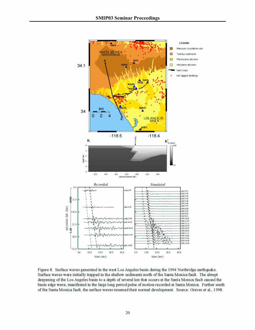
The bottom left of Figure 8 shows strong motion velocity time histories of the 1994 Northridge earthquake recorded on a profile of stations that begins in the San Fernando Valley, crosses the Santa Monica mountains and extends into the Los Angeles basin (Graves et al., 1998). The locations of the stations are shown on the map, and a geological cross section across the Santa Monica Mountains and Los Angeles basin (profile K-K’) is shown below it. The time histories recorded on rock sites in the Santa Monica Mountains (stations encr and spcn) are brief, and are dominated by direct body waves. In contrast, the time histories recorded in the Los Angeles basin (stations uclg and lacn) have much larger amplitudes and longer durations. These large waves consist of surface waves that have become trapped in the Los Angeles basin.
South of the Santa Monica fault, at station smch, even greater amplification occurs where the basin suddenly deepens across the fault. The large long period ground motions recorded at this station are due to the basin edge effect, which is illustrated schematically in Figure 7. The basin edge effect is confined to a zone that is on the order of a few km wide, lying south of the Santa Monica fault. To the south of this zone, the surface wave field resumes its normal development. The synthetic seismograms on the bottom right side of the figure, calculated using the basin structure, reproduce the features of the recorded waves. Much of the damage in the Los Angeles basin during the Northridge earthquake, including the collapse of the I10 freeway and damage to numerous large buildings in Santa Monica and West Los Angeles, is attributable to basin effects and basin edge effects.
A similar basin edge effect was responsible for a zone of extreme damage, located on the edge of the Osaka basin and aligned parallel to the fault through Kobe and adjacent cities on which the 1995 Kobe earthquake occurred (Pitarka et al., 1998). The near-fault ground motions generated by rupture directivity effects in the Kobe earthquake were further amplified by the basin edge effect. This effect was caused by the constructive interference between direct seismic waves that propagated vertically upward through the basin sediments from below, and seismic waves that diffracted at the basin edge and proceeded laterally into the basin (Kawase, 1996; Pitarka et al., 1998). The basin edge effect caused a concentration of damage in a narrow zone running parallel to the causative faults through Kobe and adjacent cities.
In both the Santa Monica and Kobe cases, the basin edge effect is caused by an abrupt lateral
contrast in shear wave velocity caused by faulting. Basin edges that have smooth concave bedrock profiles (such as those not controlled by faulting) are not expected to cause basin edge effects. Thus we expect that basin edge effects are not a general feature of basins, but instead are confined to particular kinds of basin edges. In this project, we did not have sufficient recorded data to model the basin edge effect, so the basin edge effect is not included in our model.
Comparison with the Joyner (2000) Model
Our initial approach to developing the basin model was to extend the basin effect adjustment
model of Joyner (2000) to shallower basins and to shorter periods, using data from a larger set of earthquakes and strong motion recordings from a larger number of basins. As described above, several important features in the formulation of the Joyner (2000) model were confirmed in the course of our analysis. However, other aspects of the Joyner (2000) model were not confirmed by our analysis. This may be attributable to the fact that our data set consisted of about three times as many recordings, obtained from five different basins instead of just the Los Angeles
SMIP03 Seminar Proceedings
10
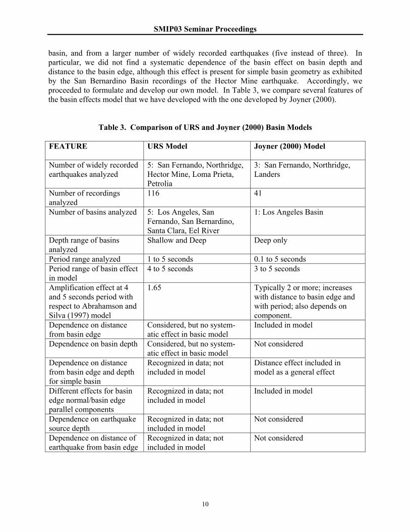
basin, and from a larger number of widely recorded earthquakes (five instead of three). In particular, we did not find a systematic dependence of the basin effect on basin depth and distance to the basin edge, although this effect is present for simple basin geometry as exhibited by the San Bernardino Basin recordings of the Hector Mine earthquake. Accordingly, we proceeded to formulate and develop our own model. In Table 3, we compare several features of the basin effects model that we have developed with the one developed by Joyner (2000).
Table 3. Comparison of URS and Joyner (2000) Basin Models FEATURE URS Model Joyner (2000) Model
Number of widely recorded earthquakes analyzed
5: San Fernando, Northridge, Hector Mine, Loma Prieta, Petrolia
3: San Fernando, Northridge, Landers
Number of recordings analyzed
116 41
Number of basins analyzed 5: Los Angeles, San Fernando, San Bernardino, Santa Clara, Eel River
1: Los Angeles Basin
Depth range of basins analyzed
Shallow and Deep Deep only
Period range analyzed 1 to 5 seconds 0.1 to 5 seconds Period range of basin effect in model
4 to 5 seconds 3 to 5 seconds
Amplification effect at 4 and 5 seconds period with respect to Abrahamson and Silva (1997) model
1.65 Typically 2 or more; increases with distance to basin edge and with period; also depends on component.
Dependence on distance from basin edge
Considered, but no system-atic effect in basic model
Included in model
Dependence on basin depth Considered, but no system-atic effect in basic model
Not considered
Dependence on distance from basin edge and depth for simple basin
Recognized in data; not included in model
Distance effect included in model as a general effect
Different effects for basin edge normal/basin edge parallel components
Recognized in data; not included in model
Included in model
Dependence on earthquake source depth
Recognized in data; not included in model
Not considered
Dependence on distance of earthquake from basin edge
Recognized in data; not included in model
Not considered

SMIP03 Seminar Proceedings
11
Conclusions We have developed a modification to the ground motion model of Abrahamson and Silva
(1997) that takes into account the effects of basin generated surface waves. Several important features in the formulation of the Joyner (2000) model were confirmed in the course of our analysis. Other aspects of the Joyner (2000) model, in particular the dependence of ground motion amplitude on basin depth and distance from basin edge, were found apply to some of the data but not to the data set as a whole. The features of our model are summarized and compared with the Joyner (2000) model in Table 3.
The main feature of our model is that for response spectral accelerations at periods of 4 and 5
seconds, the Abrahamson and Silva (1997) model for soil sites should be scaled by a factor of 1.65 in order to represent the ground motions on soil sites located within sedimentary basins.
The fact that our first order model does not have a dependence on distance to the basin edge
or the depth of the basin makes it easy to apply in ground motion calculations, especially those for probabilistic seismic hazard analyses, which typically involve the calculation of ground motions from many different scenario earthquakes occurring on a variety of faults surrounding the site. This makes our model much simpler to apply than the Joyner (2000) model, for which the distance from the source to the basin edge and the distance from the basin edge to the site must be calculated for each earthquake scenario.
For the calculation of ground motions for individual scenario earthquakes at basin sites, we
have identified a number of features that can influence the ground motions in addition to the effects of the first order model. These features, listed in Table 3, include the correlation of amplitude with distance to basin edge and depth of basin in simple basins, the difference between basin edge normal and parallel components, the depth of the earthquake, the distance of the earthquake from the basin edge, and basin edge effects. These effects are likely to depend on the location of the site within the basin, not just on the basin depth and the distance from the basin edge, and thus may best be treated using zonation of the basin rather than through the development of simple rules based on basin depth and the distance from the basin edge. The effects at a given location are also likely to depend on the location of the earthquake (Olsen, 2000), so that the zonation for basin effects needs to consider the variability caused by different earthquake locations.
References
Abrahamson, N.A. and W.J. Silva (1997). Empirical response spectral attenuation relations for shallow crustal earthquakes. Seism. Res. Lett. 68, 94-127. Building Seismic Safety Council (2001). NEHRP Recommended Provisions for Seismic Regulations for New Buildings and Other Structures, 2000 Edition. FEMA 368. Campbell, K.W. (1997). Empirical near-source attenuation relationships for horizontal and vertical components of peak ground acceleration, peak ground velocity, and pseudo-absolute acceleration response spectra. Seism. Res. Lett. 68, 154-179.

SMIP03 Seminar Proceedings
12
Field, E.H. (2000). A modified ground motion attenuation relationship for Southern California that accounts for detailed site classification and a basin depth effect. BSSA. 90, S209-S221. Graves, R.W. and D.J. Wald (2003). Observed and simulated ground motions in the San Bernardino basin region for the Hector Mines earthquake. Bull. Seism. Soc. Am., 93, in press. Graves, R. W., A. Pitarka, and P. G. Somerville (1998). Ground motion amplification in the Santa Monica area: effects of shallow basin edge structure. Bull. Seism. Soc. Am., 88, 1258-1276. Graves, R.W. (1996). Simulating seismic wave propagation in 3D elastic media using staggered grid finite differences, Bull. Seism. Soc. Am., 86, 1091-1106. Hruby, C. and I. Beresnev (2002). Empirical corrections for basin effects in stochastic ground motion prediction. Eos Trans. AGU, Abstract S12B-1223. International Conference of Building Officials (1997). Uniform Building Code, 1997 Edition. Joyner, W.B. (2000). Strong motion from surface waves in deep sedimentary basins. Bull. Seism. Soc. Am., 90, S95-S112. Kawase, H., The cause of the damage belt in Kobe, the “basin edge effect,” constructive interference of the direct S-wave with the basin-induced diffracted/Rayleigh waves. Seism. Res. Lett., 67, No.5, 25-34. Lee, Y. and J.G. Anderson (2000). Potential for improving ground motion relations in Southern California by incorporating various site parameters. Bull. Seism. Soc. Am. 90, S170-S186. Olsen, K.B. (2000). Site amplification in the Los Angeles Basin from three-dimensional modeling of ground motion. Bull. Seism. Soc. Am., 90, S77-S94. Pitarka, A. (1999). 3D finite-difference modeling of seismic motion using staggered grid with non-uniform spacing, Bull. Seism. Soc. Am., 89, 54-68. Pitarka, A., K. Irikura, T. Iwata and H. Sekiguchi (1998). Three-dimensional simulation of the near-fault ground motion for the 1995 Hyogo-ken Nanbu (Kobe), Japan, earthquake. Bull. Seism. Soc. Am., 88, 428-440. Trifunac, M.D. and V.W. Lee (1979). Dependence of pseudo-relative velocity spectra of strong ground motion acceleration on the depth of sedimentary deposits. Rept. No. CE79-02, Dept. of Civil Engineering, University of Southern California, Los Angeles. Vidale, J.E. and D.V. Helmberger (1988). Elastic finite-difference modeling of the 1971 San Fernando, California earthquake. Bull. Seism. Soc. Am., 78, 122-141. Wald, D.J. and R.W. Graves (1998). The seismic response of the Los Angeles basin, California. Bull. Seism. Soc. Am., 88, 337-356.
SMIP03 Seminar Proceedings
13

SMIP03 Seminar Proceedings
14

SMIP03 Seminar Proceedings
15

SMIP03 Seminar Proceedings
16

SMIP03 Seminar Proceedings
17

SMIP03 Seminar Proceedings
18

SMIP03 Seminar Proceedings
19
SMIP03 Seminar Proceedings
20

SMIP03 Seminar Proceedings
21
DESIGN GROUND MOTION LIBRARY: A PROGRESS REPORT
Maurice S. Power Geomatrix Consultants, Inc., Oakland, California
Abstract
A Design Ground Motion Library (DGML) is being developed that will contain selected recorded acceleration time histories considered to be suitable for use by engineering practitioners for the time history dynamic analysis of various facility types in California and other parts of the Western United States. The DGML will include: (1) the electronic library of selected time histories and their associated ground motion parameters and supporting information on the earthquake source, travel path, and site characteristics; and (2) detailed guidelines for forming and scaling sets of time histories for applications. The characteristics of the seismic environment, including earthquake magnitude, faulting mechanism, source-to-site distance, near-fault directivity conditions, and site conditions, and the damaging characteristics of time histories are being incorporated into criteria for selecting and binning records for the library.
Introduction
This paper presents a progress report on the development of a Design Ground Motion Library (DGML) of recorded acceleration time histories of ground motion suitable for use by engineering practitioners for time-history analysis of various facility types in California and other parts of the western United States. The DGML project is jointly sponsored by the California Strong Motion Instrumentation Program (CSMIP) and the Pacific Earthquake Engineering Research Center (PEER)-Lifelines Program. The project was initiated in August 2002 and extends through December 2003. Currently, there are a number of data bases of ground motion time histories recorded during earthquakes, e.g. PEER, COSMOS, CSMIP, and USGS. These data bases contain large numbers of ground motion records but do not provide guidance to the engineering practitioner as to how to select sets of records for time history analyses for specific facilities. In contrast to a data base, the DGML will comprise a smaller collection of records considered to be especially suitable for applications along with guidelines for assembling and scaling sets of records for these applications. The DGML is currently limited to recorded time histories from shallow crustal earthquakes of the types that occur in the western United States. Time histories recorded during subduction zone earthquakes will not be part of the library during this project. However, the project sponsors envision that future development of the DGML will add records from subduction zone earthquakes (appropriate for these types of earthquakes occurring in northwest California, Oregon, Washington, and Alaska) and will also supplement recorded motions with time histories simulated by seismological ground motion modeling methods.

SMIP03 Seminar Proceedings
22
The principal strategy in conducting the project is to utilize a team that is expert in selection and use of time history records to develop the criteria for the DGML, select the records for the DGML using the criteria and judgment, and develop guidelines for utilizing the DGML for applications. Accordingly, a multi-disciplinary project team of practitioners and researchers in structural engineering, geotechnical engineering, and seismology is conducting the project. The team comprises expertise in the time history dynamic analysis of building, bridges, dams, other heavy civil structures, lifeline structures and systems, and base isolated structures. The project team includes the following organizations and individuals: Geomatrix Consultants, Inc., prime contractor (Maurice Power, Robert Youngs, and Faiz Makdisi); Simpson Gumpertz & Heger, Inc. (Ronald Hamburger and Ronald Mayes); T.-Y. Lin International (Roupen Donikian); Quest Structures (Yusof Ghanaat); Pacific Engineering & Analysis (Walter Silva); URS Corporation (Paul Somerville); Earth Mechanics (Ignatius Po Lam); Professor Allin Cornell, Stanford University; and Professor Stephen Mahin, University of California, Berkeley.
Specific Project Objectives and Tasks
The specific objectives of the DGML project are:
(1) To develop an electronic Design Ground Motion Library containing the selected ground motion time histories.
(2) To develop utilization guidelines for forming and scaling time history record sets for applications.
(3) To identify the limits of applicability and deficiencies of the DGML and provide recommendations for further development.
The primary tasks being undertaken to achieve the objectives are:
Task 1 - Review of previous relevant efforts and information. Task 2 - Development of criteria for the DGML. Task 3 - Selection, analysis, and placement of records in the DGML based on the developed criteria and judgment. Task 4 - Development of utilization guidelines for the DGML Task 5 - Testing, evaluation, and finalization of the DGML Task 6 - Preparation of final report including recommendations for further development.
Task 1 includes: review of existing ground motion libraries and databases; review of current knowledge of time history characteristics important to structure response and performance; and review of current practice and existing guidelines for selecting and scaling time history records. These reviews have been conducted and are continuing, especially with
SMIP03 Seminar Proceedings
23
regard to ongoing research on the relation of time history characteristics and structure performance.
The principal tasks are 2, 3, and 4. Criteria development for the DGML, Task 2, is in progress, and the selection of records in Task 3 will utilize the results of that task. Preliminary work has been done on utilization guidelines, Task 4. Tasks 2 and 4 are discussed in sections below. Task 5 provides for the project team and selected other users to conduct trial usage of the DGML so that modifications can be made to the electronic package and the utilization guidelines during the DGML finalization process.
Criteria Development
Elements of criteria for the DGML are: time history record characteristics to be quantified; supporting information on records to be included; structure of the DGML; and criteria for including or excluding records in the DGML.
Record Characteristics It is desirable, but not necessarily essential, that characteristics or parameters of records selected to be quantified for records in the DGML satisfy two criteria: First, the parameters should be known to correlate with structural or ground performance, thus permitting records to be selected with knowledge of their relative damageability. Second, the parameters should be definable as a function of the seismic environment such as magnitude, distance, type of faulting, and subsurface site conditions; that is, attenuation relationships for the parameters should be available.
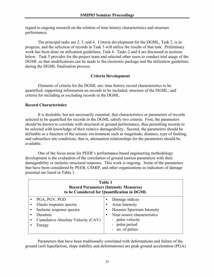
One of the focus areas for PEER’s performance-based engineering methodology development is the evaluation of the correlation of ground motion parameters with their damageability or inelastic structural response. This work is ongoing. Some of the parameters that have been considered by PEER, CSMIP, and other organizations as indicators of damage potential are listed in Table 1.
Table 1
Record Parameters (Intensity Measures) to be Considered for Quantification in DGML
• PGA, PGV, PGD • Elastic response spectra • Inelastic response spectra • Duration • Cumulative Absolute Velocity (CAV) • Energy
• Damage indices • Arias Intensity • Housner Spectrum Intensity • Near-source characteristics
- pulse velocity - pulse period - no. of pulses
Parameters that have been traditionally correlated with deformations and failure of the ground (soil liquefaction, slope stability and deformations) are peak ground acceleration (PGA)
SMIP03 Seminar Proceedings
24
and duration of shaking (the latter typically quantified as the time to build up a fraction of the Arias Intensity, Ia , of a time history, say the time to buildup from 5% to 95% or from 5% to 75% of Ia ). Kramer and Mitchell (2003), in studies for PEER, proposed the use of cumulative absolute velocity (CAV) as a parameter correlated with the development of excess pore water pressure and liquefaction in soils. Travasarou et al. (2003), also in studies for PEER, proposed the use of Arias Intensity as a parameter correlated with damage to stiff systems such as short-period structures and stiff soil slopes. Both CAV and Ia contain the effects of ground motion duration as well as amplitude because the parameters are summed over the duration of the time history.
A number of studies by PEER and PEER-Lifelines Program have indicated the strong correlation between structure damageability and elastic response spectral characteristics, either at the fundamental period of a structure or at a discrete number of periods or over a period range in order to capture ground motion intensity for higher modes of vibration (shorter periods), or at longer periods reflecting structural softening as damage occurs (e.g., Shome et al., 1998; Cordova et al., 2001; Luco and Cornell, 2003; Bazzurro and Luco, 2003; Cornell, 2003; Jalayer, 2003).
Inelastic response spectra have been found to improve the prediction of inelastic response and damage in some studies by PEER and PEER-Lifelines Program (e.g. Luco and Cornell, 2003; Bazzurro and Luco, 2003). Damage indices or damage spectra combining different measures of inelastic response (e.g. ductility and hysteretic energy) may also improve predictions of damageability (e.g. Bozorgnia and Bertero, 2002, in studies for CSMIP).
Near-source time history record characteristics, i.e. the strong pulsive ground motion characteristics associated with fault rupture directivity toward a site especially for the fault-strike-normal component of motion (e.g. pulse velocity, pulse period, and number of pulses) have been shown to be very damaging in studies by Krawinkler and Alavi (1998) for CSMIP. In-progress studies by Bazzurro and Luco (2003) for PEER-Lifelines Program have not shown a significant improvement in damage predictability associated with pulse period or velocity over the correlation with elastic response spectral characteristics alone for a data set of spectrum-matched near-source time histories.
The preceding are only a few examples of studies of time history characteristics related to structure damageability. To date, except for strong evidence that the elastic response spectrum and response spectral shape are strongly correlated with inelastic structural response (by virtue of their capturing the intensity of ground motions at structural periods of significance), there does not seem to be a strong consensus on the degree to which other parameters improve damage predictions. The importance of other parameters may be very structure-dependent. Knowledge in this area may be expected to increase rapidly.
With regard to ground motion attenuation relationships available to date to predict the parameters in Table 1 as a function of the seismic environment and site conditions, such relationships are available only for PGA, PGV, elastic response spectra, duration, Arias Intensity, and to a more limited degree, for near-source ground motion pulse characteristics.
SMIP03 Seminar Proceedings
25
Knowledge of the relationships of the parameters in Table 1 with damage and development of attenuation relationships for these parameters will increase with time. Therefore, the approach in the DGML project will be to quantify for time histories in the DMGL all of the parameters in Table 1 that are considered by the project team as potentially useful in damage estimation for some structure types or in ground failure estimation. Some of the parameters have multiple definitions or formulations (e.g. inelastic response spectra, energy, damage indices), and the specific definitions will need to be selected.
Supporting Information
Table 2 summarizes the types of supporting information that will be included for the records in the DGML. This information pertains to the parameters of the causative earthquake, source-to-site travel path, and site conditions at the ground motion recording station. Currently, supporting information for records in the PEER strong motion data base is being updated and added to as part of a project sponsored by PEER-Lifelines Program, USGS, and SCEC to develop next-generation attenuation relationships for western U.S. shallow crustal earthquakes (NGA project). The updated and additional information, to be available this summer, will be included for records placed in the DGML.
Table 2
Supporting Information about Records to be Quantified in DGML
• Earthquake magnitude • Faulting mechanism • Hanging wall vs. foot wall • Source-to-site distance
• Near-fault directivity parameters • Site classification(s) • Basin response influence
The near-fault directivity parameters referred to in Table 2 are important for records within 15 to 20 km of the causative earthquake. The parameters to be summarized are those defined by Somerville et al. (1997) and include those illustrated in Figure 1; additional parameters may be added based on the PEER data base update for the NGA project.
Structure of the DGML It is planned that the basic structure of the DGML will be based on parameters of the seismic hazard environment. That is, records will be grouped or “binned” based on the earthquake source, travel path, and site conditions for the records. Currently, it is planned that records will be binned within the earthquake magnitude and closest source-to-site distance ranges shown in Table 3. Separate sets of bins will be formed for different site conditions (most likely “firm soil” and “rock” sets) and may be formed for different faulting mechanisms (strike-slip, reverse, normal). The overlapping of the two highest magnitude bins (6.5 - 7.0 and 6.9 - 7.9) is for the purpose of reducing the dominance of the M 7.6 Chi-Chi, Taiwan earthquake in the highest magnitude bin by including M6.9 recordings from the 1989 Loma Prieta, 1992 Erzican, and 1995 Kobe earthquakes in both bins. It is likely that the near-source bins will be defined as overlapping into the 10 to 25 km bin in order to bring in records with near-source ground motion characteristics as far as 15 to 20 km from the earthquake source.

SMIP03 Seminar Proceedings
26
Table 3
Preliminary Hazard Bin Ranges for DGML
Moment Magnitude
Earthquake Closest Source-to-Site Distance (km)
5.0 – 5.9 0 – 10, > 10 – 25, > 25 - 50 6.0 – 6.4 0 – 10, > 10 – 25, > 25 - 50 6.5 – 7.0 0 – 10, > 10 – 25, > 25 – 50, > 50 – 100 6.9 – 7.9 0 – 10, > 10 – 25, > 25 – 50, > 50 - 100
As discussed in the following section, sub-bins within the basic hazard bin structure may be formed for structural parameters or characteristics of interest.
Record Inclusion/Exclusion Criteria
A complete set of criteria for including records in, or excluding records from, the DGML, including the number of records in each bin, has not been finalized. Because of the importance of response spectral content and response spectral shape, it is planned to include as part of the criteria the shape of the spectrum of the recorded time history in comparison to the median shape for a particular hazard bin as determined by established ground motion attenuation relationships. The shape would be defined for a number of period ranges defined to encompass period ranges of interest for a wide range of structures. Sub-bins would be formed for record sets selected for each period range. Some records would be in multiple sub-bins. Preliminary period ranges selected for the sub-bins are shown in Table 4.
Within a given sub-bin, all records within the hazard bin (for example rock records in the magnitude range 6.5 - 7.0 and distance range 10 - 25 km) would be scaled to “fit” the median target spectrum calculated from attenuation relationships for the central magnitude and distance of that bin (for example M 6.75, distance 17.5 km). The fit for a given time history corresponds to equal differences of the record spectrum above and below the target spectrum. Then, a subset of records for the library (for the particular sub-bin) could be selected as some number of records having the closest overall “match” to the target spectrum. The closest match corresponds to the minimum mean of squared differences between the record spectrum and the target spectrum.
Table 4 Preliminary Period Sub-Bin Ranges For DGML
(seconds)
0.1 – 0.5 0.1 – 1.0 0.2 – 4.0 0.5 – 1.5
0.5 – 4 1 – 3 2 – 4
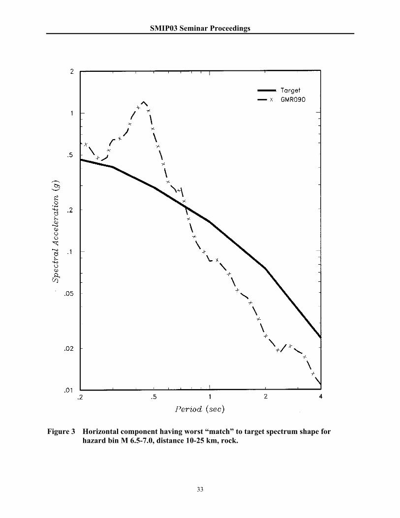
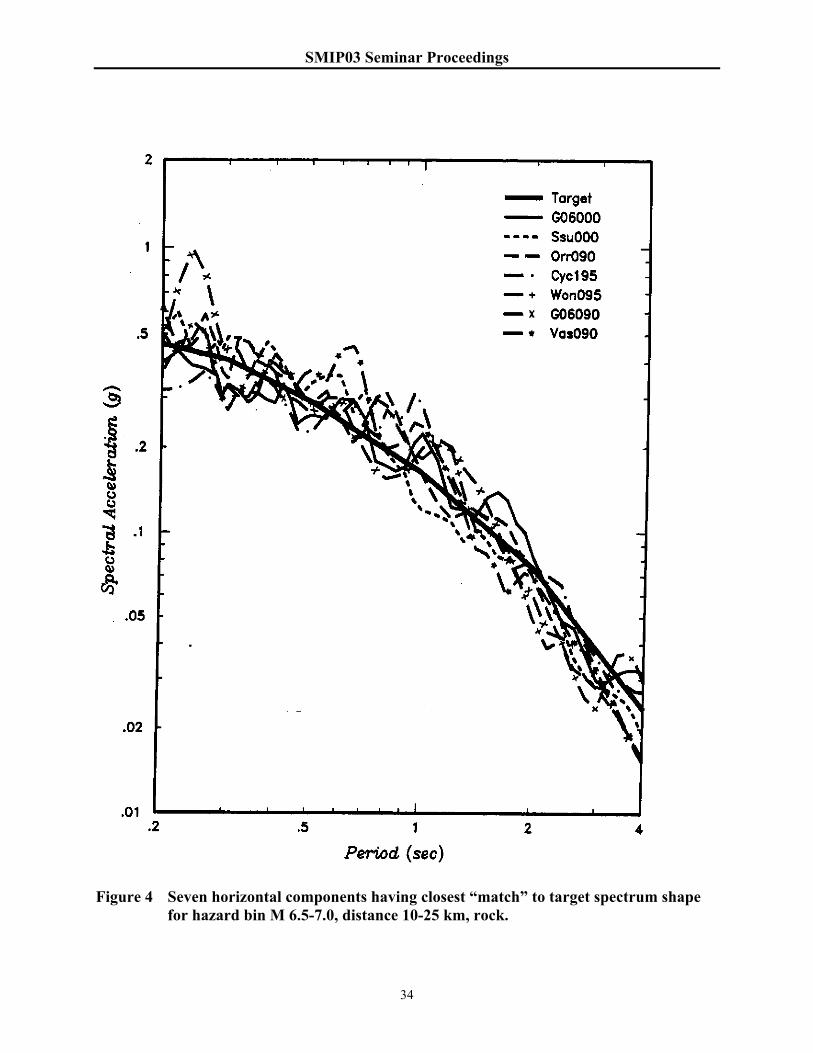
Figures 2, 3, and 4 illustrate a trial application of this binning procedure for the period range 0.2 to 4.0 seconds within the rock record bin of M 6.5 - 7.0, distance 10 - 25 km. There

SMIP03 Seminar Proceedings
27
are a total of 40 horizontal ground motion time histories within this hazard bin (before excluding any records). In Figure 2, the spectrum of the time history having the closest match to the target spectrum is compared with the target spectrum. The target spectrum was constructed using the Abrahamson and Silva (1997) attenuation relationship. In Figure 3, a similar comparison is made for the spectrum of the time history having the worst match. Figure 4 illustrates the selection of seven time histories that have the closest match to the target spectrum shape.
For application where the ground motion is defined on the basis of a probabilistic seismic hazard analysis (PSHA), the dominant (mean or mode) magnitude and distance would be determined by deaggregation of the probabilistic hazard, and the set of time histories having the closest match would be selected from the corresponding hazard bin and the sub-bin for a selected period range. These records would then be further scaled to the actual design spectrum determined from the PSHA.
There are many aspects to be decided with respect to the criteria for the DGML, including the total set of selection criteria to be applied and the details of the criteria. Certainly, within the near-source bins, criteria should include consideration of seismological directivity parameters (Figure 1). The overall goal is to form “representative” time history sets that, in aggregate, are representative of the expected or average hazard conditions for a project site.
Where it is desired that a broad range of potential variability be included in a selected record set, consideration can also be given to including randomly selected records from the hazard bins.
Utilization Guidelines
Table 5 summarizes topics for which utilization guidelines will be developed for scaling records to be the level of the actual design response spectrum after record sets have been selected. There are two types of scaling: (1) simple scaling by a constant factor; and (2) spectrum matching using techniques that adjust the frequency content of a time history so that the spectral peaks and valleys of the record are largely eliminated and the resulting spectrum is a close fit to a smooth design spectrum. There are pros and cons to each type of scaling and advocates for each. Both types of scaling will be covered in the guidelines with the pros and cons indicated and the procedures for implementation of the topics in Table 4 described in detail. PEER and PEER-Lifelines Program have been and are investigating these topics. For example, Shome et al. (1998) and Cornell (2003) reported on the insensitivity of inelastic response to varying amounts of simple scaling of records to the level of the design spectrum, and Carballo and Cornell (2000) and Bazzurro and Luco (2003) have conducted studies that indicate that spectrum matching biases inelastic response somewhat to the low side in comparison to response using simple scaling. Such studies will be further considered during the development of utilization guidelines.

SMIP03 Seminar Proceedings
28
Table 5
Topics for Utilization Guidelines for the DGML, Simple Scaling and Spectrum Matching Approaches
Simple scaling approach (by constant factor) - guideline limits on scaling factors - number of records - guidelines on aggregate “match” of scaled record parameters to design values - guidelines for scaling records for 2-component or 3-component dynamic analysis
Spectrum matching approach - advantages and limitations of spectrum matching versus simple scaling - guidelines for the spectrum matching process
- similarity of spectrum shape of record and design spectrum - scaling before matching - acceptable spectrum matching methods (frequency and time domains) - tolerances for spectrum matching fit and number of periods for evaluating
- number of records
Summary
Evaluations to date by the project team indicate that binning of records for the DGML should principally be based on seismic hazard (as principally indicated by earthquake magnitude and distance ranges and site conditions). The evaluations also indicate that with the current state of knowledge, an important criterion for selecting subsets of records for the DGML within defined hazard bins should be the elastic response spectral shape over a period range of significance for a specific structure. Work to date has tentatively defined hazard bins and a procedure for selecting record subsets that, when scaled, will have response spectral shapes that are most consistent with a target spectrum shape that is representative of the hazard bin. Within near-source distances (say within 15 km to 20 km of the earthquake source), record selection criteria should also include the time-domain pulsive characteristics of records and earthquake rupture directivity conditions that produced the near-source ground motion characteristics. Both within and outside the near-source region, it is currently not clear which ground motion characteristics other than the characteristics mentioned above should comprise part of general DGML record selection criteria. However, duration of shaking and inelastic response spectral characteristics appear to be ground motion characteristics that warrant consideration. The difficulties of using many ground motion parameters as part of the general record selection criteria are, at present, two-fold: (1) the importance of the parameter to structure damageability may not be clear, and the knowledge is evolving; and (2) ground motion attenuation relationships to predict the values of those parameters as a function of the seismic hazard environment (e.g., magnitude, distance, local site conditions, etc.) have not yet been developed for most of the parameters in Table 1, thus it may not be clear what constitutes a

SMIP03 Seminar Proceedings
29
“high”, “low”, or “average” parameter value for a given seismic environment. Nevertheless, further consideration will be given to how other time history characteristics may be incorporated into record selection criteria. It is straightforward to quantify for individual time history records many of the ground motion parameters of potential interest to a designer for a specific project (e.g. parameters listed in Table 1). For records placed in the library, it is planned to quantify many of these parameters, as selected by the project team members and reviewed by advisors representing CSMIP and PEER-Lifelines Program, so that these characteristics of records can be considered by users of the library, whether or not the parameters are part of general record selection criteria. Detailed guidelines will be developed for using the DGML to assemble and scale record sets for applications. Scaling approaches to be addressed include simple scaling and spectrum matching. The topics listed in Table 5 will be addressed in these utilization guidelines.
References
Abrahamson, N.A., and Silva, W.J., 1997, Empirical response spectral attenuation relations for shallow crustal earthquakes: Seismological Research Letters, v. 68, no. 1, p. 94-127. Bazzurro, P. and Luco, N. 2003, Parameterization of non-stationary time histories, Report for Task 1G00 to PEER-Lifelines Program (in preparation). Bozorgnia, Y. and Bertero, V.V., 2002, Improved damage parameters for post-earthquake applications, Proceedings SMIP02 Seminar on Utilization of Strong-Motion Data, Los Angeles, California Strong Motion Instrumentation Program, California Geological Survey, p. 61-82. Carballo, J.E., and Cornell, C.A., 2000, Probabilistic seismic demand analysis: spectrum matching and design, Report No. RMS-41, Department of Civil and Environmental Engineering, Stanford University. Cornell, A., Jalayer, F., Iervolino, I., and Baker, J., 2003, Record selection for nonlinear time history analysis, Presentation at PEER Annual Meeting, Palm Springs, California. Jalayer, F., 2003, Direct probabilistic seismic analysis: implementing non-linear dynamic assessments, PhD thesis, Department of Civil and Environmental Engineering, Stanford University. Kramer, S. and Mitchell, R., 2002, Liquefaction intensity measure, paper prepared for PEER review meeting. Krawinkler, H., and Alavi, B., 1998, Development of improved design procedures for near-fault ground motions, Proceedings SMIP98 Seminar on Utilization of Strong-Motion Data, Oakland, California Strong Motion Instrumentation Program, California Geological Survey, p. 21-41.
SMIP03 Seminar Proceedings
30
Luco, N., and Cornell, C.A., 2003, Structure-specific scalar intensity measures for near-source and ordinary earthquake ground motions, paper under revision for Earthquake Spectra. Shome, N. Cornell, C.A., Bazzurro, P., and Carballo, J.E., 1998, Earthquake records and nonlinear response, Earthquake Spectra, v. 14, no. 3, p. 469-500. Somerville, P.G., Smith, N.F., and Graves, R.W., 1997, Modification of empirical strong ground motion attenuation relations to include the amplitude and duration effects of rupture directivity: Seismological Research Letters, v. 68, no. 1, p. 199-222. Travasarou, T., Bray, J. D., and Abrahamson, N. A., 2003, Empirical attenuation relationship for Arias Intensity, Journal of Earthquake Engineering and Structural Dynamics, v. 32, pp. 1133-1155.

SMIP03 Seminar Proceedings
31
Figure 1 Definition of rupture directivity parameters Ө, s, and X for strike-slip faults, and
Ø, d, and Y for dip-slip faults, and region off the end of dip-slip faults excluded from the model (Somerville et al., 1997).

SMIP03 Seminar Proceedings
32
Figure 2 Horizontal component having closest “match” to target spectrum shape for
hazard bin M 6.5-7.0, distance 10-25 km, rock.
SMIP03 Seminar Proceedings
33
Figure 3 Horizontal component having worst “match” to target spectrum shape for
hazard bin M 6.5-7.0, distance 10-25 km, rock.
SMIP03 Seminar Proceedings
34
Figure 4 Seven horizontal components having closest “match” to target spectrum shape
for hazard bin M 6.5-7.0, distance 10-25 km, rock.

SMIP03 Seminar Proceedings
35
UTILIZING STRONG-MOTION DATA AFTER EARTHQUAKES: UPDATE ON THE CISN ENGINEERING DATA CENTER,
INTERNET QUICK REPORT, SHAKEMAP AND CISN DISPLAY
Anthony Shakal, Kuo-Wan Lin, and Moh Huang Strong Motion Instrumentation Program, California Geological Survey
Christopher Stephens and Woody Savage
National Strong Motion Program, U.S. Geological Survey
Egill Hauksson and Hugo Rico California Institute of Technology
Introduction
The California Integrated Seismic Network (CISN) is a consortium of institutions
engaged in statewide earthquake monitoring. The five core members are the California Geological Survey, the California Institute of Technology, the U.S. Geological Survey Offices at Pasadena and Menlo Park, and UC Berkeley. The California Office of Emergency Services (OES) participates as an ex-officio participant. The TriNet project initiated in southern California with FEMA support was a prototype for the statewide CISN project.
The CISN has a statewide Engineering Data Center, a southern California seismic Data Center at Pasadena, and a northern California seismic Data Center in the Bay area. The CISN Engineering Data Center is operated by the CGS Strong Motion Instrumentation Program (CSMIP) in cooperation with the USGS National Strong Motion Program (NSMP).
A primary goal of the Engineering Data Center as well as the other two Data Centers is to provide robust and rapid information products after an earthquake, with products ranging from the ShakeMap to strong-motion data and calculated parameters. A high-speed T-1 computer communication network, or Intranet, which connects all CISN partner agencies has been recently established, depicted in Figure 1. The T-1 communication ring consists of dedicated segments connecting each center and OES, and is completely independent of the Internet. The ring became operational early in 2003. The Internet is also used in communication between the centers, but the T-1 ring provides the secure, reliable backup to the Internet that is needed. A second level of backup, using OES satellite communication channels, is also planned.
Effective communication requires standardized protocols. Data packets and formats for
the exchange of parametric data and waveforms are being finalized by the CISN Program Management Committee and its Standards Committee. With the completion of the T-1 ring, the CISN partners have begun routine exchange of strong-motion parametric data between centers while the protocols for exchange of waveforms are being standardized. When routine waveform exchange begins, planned for later in 2003, it will be possible to assemble the strong-motion data for all strong-motion stations in the State at CISN, in forms convenient for use by the earthquake engineering or seismology communities, an unprecedented advance.

SMIP03 Seminar Proceedings
36
Figure 1. Communication pathways between seismic centers within the CISN system. The
dedicated T1 segments form a robust ring, with communication allowed in both directions in the event one segment is damaged. Normal communication tunnels through the Internet cloud are also used, but as backup to each link of the robust system.
The Engineering Data Center The Engineering Data Center is at URL http://www.cisn-edc.org (Figure 2) and
additional mirror sites are planned at CGS and USGS in the future. These will provide the critically needed robustness and redundancy, in the case of a major earthquake or other disabling event at either Sacramento or Menlo Park, a central goal of the CISN and of OES.
The Internet Quick Report The EDC uses the Internet Quick Report (IQR) to rapidly disseminate strong-motion data for engineering applications after major earthquakes. The IQR is based on the concept of the traditional Quick Report, streamlined for automated generation. A total of 13 IQRs have been released after earthquakes of M~4 and larger since August 2001. In addition, a search function
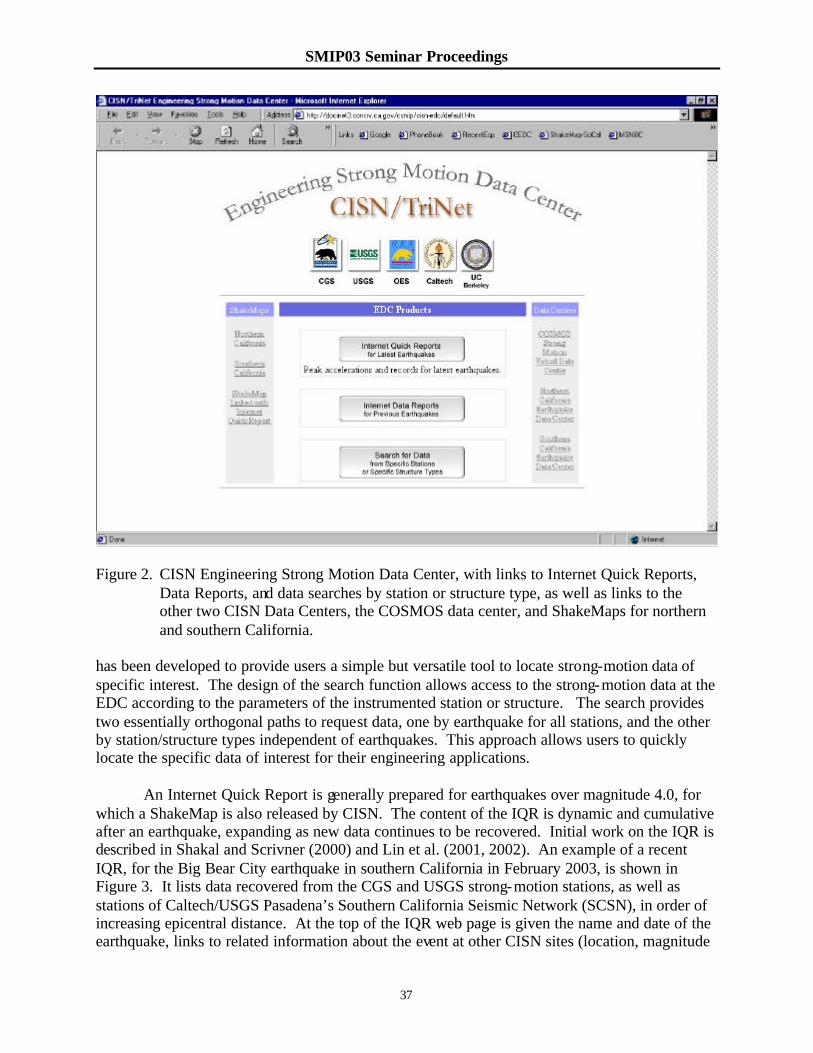
SMIP03 Seminar Proceedings
37
Figure 2. CISN Engineering Strong Motion Data Center, with links to Internet Quick Reports,
Data Reports, and data searches by station or structure type, as well as links to the other two CISN Data Centers, the COSMOS data center, and ShakeMaps for northern and southern California.
has been developed to provide users a simple but versatile tool to locate strong-motion data of specific interest. The design of the search function allows access to the strong-motion data at the EDC according to the parameters of the instrumented station or structure. The search provides two essentially orthogonal paths to request data, one by earthquake for all stations, and the other by station/structure types independent of earthquakes. This approach allows users to quickly locate the specific data of interest for their engineering applications.
An Internet Quick Report is generally prepared for earthquakes over magnitude 4.0, for which a ShakeMap is also released by CISN. The content of the IQR is dynamic and cumulative after an earthquake, expanding as new data continues to be recovered. Initial work on the IQR is described in Shakal and Scrivner (2000) and Lin et al. (2001, 2002). An example of a recent IQR, for the Big Bear City earthquake in southern California in February 2003, is shown in Figure 3. It lists data recovered from the CGS and USGS strong-motion stations, as well as stations of Caltech/USGS Pasadena’s Southern California Seismic Network (SCSN), in order of increasing epicentral distance. At the top of the IQR web page is given the name and date of the earthquake, links to related information about the event at other CISN sites (location, magnitude
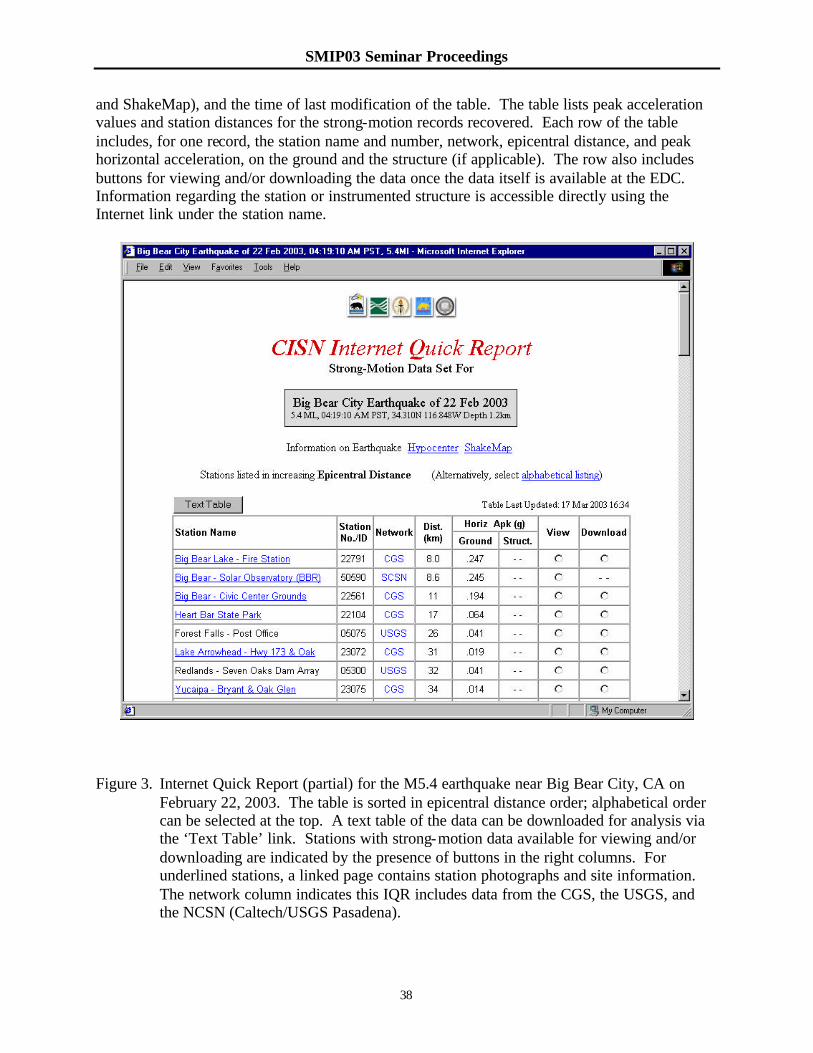
SMIP03 Seminar Proceedings
38
and ShakeMap), and the time of last modification of the table. The table lists peak acceleration values and station distances for the strong-motion records recovered. Each row of the table includes, for one record, the station name and number, network, epicentral distance, and peak horizontal acceleration, on the ground and the structure (if applicable). The row also includes buttons for viewing and/or downloading the data once the data itself is available at the EDC. Information regarding the station or instrumented structure is accessible directly using the Internet link under the station name.
Figure 3. Internet Quick Report (partial) for the M5.4 earthquake near Big Bear City, CA on February 22, 2003. The table is sorted in epicentral distance order; alphabetical order can be selected at the top. A text table of the data can be downloaded for analysis via the ‘Text Table’ link. Stations with strong-motion data available for viewing and/or downloading are indicated by the presence of buttons in the right columns. For underlined stations, a linked page contains station photographs and site information. The network column indicates this IQR includes data from the CGS, the USGS, and the NCSN (Caltech/USGS Pasadena).

SMIP03 Seminar Proceedings
39
The table shown, designed for viewing using Internet browsers, is complemented by a more comprehensive table available as an ASCII text file using a link at the top of the page. A user can easily import this table into a spreadsheet program for analysis. Both the web table and the text table have a date-time stamp to indicate when they were last modified by the update or addition of data.
Linking the Internet Quick Report and ShakeMap
The ShakeMap and the Internet Quick Report are CISN products that use the data from the same strong motion stations. The data inputs for the ShakeMap consist of parametric data (peak ground acceleration, velocity, and spectral accelerations) for the record from a station, while the IQR also includes time history data. In an effort to provide users easy access to both CISN products, the EDC has developed links to the time history plots of the IQR from within the ShakeMap.
Figure 4 shows the ShakeMap for the Big Bear City earthquake of February 22, 2003. As
shown in the figure, the pop-up window in the upper left corner contains values of peak ground motion and station related information from a specific station as in the standard ShakeMap. In addition, an EDC extension includes a hypertext link for the station for direct access to the time history plot for the same station in the IQR. Clicking the hypertext link causes a new window to appear on the screen with the IQR time history plot displayed side by side with the ShakeMap. In the example this has been done for two different stations on the same screen. This implementation allows engineering users to navigate between the two products more efficiently.
The creation and update of the station links inside the ShakeMap is an add-on process of
the IQR. This means that the update is also dynamic and cumulative like the update of the IQR. Not all ShakeMaps will contain links to the time history plots at the EDC since the criteria for the production of ShakeMaps and IQRs may be different.
Data for Previous Earthquakes – Internet Data Reports
The discussion above is focused on data in the immediate post-earthquake period.
Earthquake data is also important for longer-term analysis, beyond the immediate earthquake response time frame. In the past, paper-copy Quick Reports (e.g., CSMIP, 1994) were the pre-Internet analog to the Internet Quick Reports, and those Quick Reports were followed by a final, hard-copy report on the event’s strong motion data, which was usually released one month after the event (e.g., Shakal et al., 1994; Porcella et al., 1994). In many ways, the IQR is as comprehensive as that report; thus, using new technology, a product is being produced in 30 minutes, which is very comparable to what was available only after 30 days. For a given event, the Internet Quick Report will transition to the Internet Data Report, to reflect its more final nature, after enough time has gone by for all data (including that from any analog instruments) to be included and quality controlled.
The EDC has created Internet Data Reports for four major historical earthquakes, to provide users the same access to the earlier strong-motion data as for new data. More historical

SMIP03 Seminar Proceedings
40
earthquakes are being added. An example showing part of the Internet Data Report for the 1994 Northridge earthquake is shown in Figure 5. The Internet Data Reports have the same format as the IQR and are placed in the archive section of the EDC, paralleling the way the CISN ShakeMaps are archived. Internet Data Reports are being created for additional historical earthquakes as current data work allows.
Figure 4. The ShakeMap for the Big Bear City earthquake of February 22, 2003 at the CISN
Engineering Data Center. The ShakeMap is linked with the Internet Quick Report (IQR) and screens with the time history plots from the IQR can be accessed directly from within the ShakeMap.

SMIP03 Seminar Proceedings
41
Figure 5. An example of the Internet Data Report table, sorted in epicentral distance order, for the M6.7 Northridge of Jan 17, 1994. The table parallels the functionality of the Internet Quick Report, but is permanently available, beyond the time of post-earthquake response, and includes records from analog film stations and other records that may be recovered manually (this is an example and only includes CGS data).
Searching for Strong-Motion Data at the CISN Engineering Data Center
The design goal of the EDC search function is the distribution of strong-motion data from
stations of the CISN network in a rapid manner and the provision of station information and associated structural information, as applicable. It complements the worldwide ground-response database available through the COSMOS virtual data center (e.g., Archuleta, 2000) and the newly completed Internet Site for European Strong Motion Data (Ambraseys, 2000).

SMIP03 Seminar Proceedings
42
The layout of the EDC search function is a typical top-down tier approach that guides the
user through a series of choices. The user can further confine the search criteria by entering keywords in appropriate fields anytime during the search process. Results of a given search are presented in a table listing all stations that matched the search criteria. Each station has a direct link in the result table that leads the user to a list of readily accessed strong-motion data for the station.
In 2002-2003, more earthquakes and station data were added to the EDC. The
functionality of the search feature was improved to incorporate the newly added data. Currently, data for all 13 Internet Quick Reports and four Internet Data Reports of historic earthquakes have been entered into the database. In addition, station information on all ground response stations and approximately one third of the building stations has been loaded into the EDC search feature. The EDC is continuing to work with the CISN partners to increase the inventory of information for the CISN stations.
With the inventory of the ground response stations nearly complete, it is now possible to
search for station information for most ground response stations and for the earthquake data associated with the stations. Users can take advantage of the search feature to obtain information on a single station or group of stations based on the geographical location, such as city name. Figure 6 shows the result of a sample search that lists the ground response stations in the city of Los Angeles.
ShakeMap Utilization
The ShakeMap product, developed under TriNet, provides a graphical portrayal of the regional shaking (Wald et al., 1999) for use in rapid post event response. Another level of utilization of the ShakeMap by engineers is in guiding the assessment of structural performance and structural safety after an event. The strong motion data itself, in addition to the information captured in ShakeMaps, is also important. Rojahn et al (2003) describe the ATC-54 report by the Applied Technology Council focused on these engineering applications. This is an important progression in increasing the usefulness of ShakeMap.
Another important application of ShakeMap is in engineering loss estimation. HAZUS, a
project of FEMA and the National Institute of Building Sciences (NIBS) is an advanced computational methodology to estimate loss after a significant earthquake. With the introduction of ShakeMap, is becomes possible to do loss estimation in near real time. HAZUS was conceived in a time when rapid data was not available, so ShakeMap expands its value, as well as increases the importance of calibration of methodology and inventory in order for the results, produced rapidly and possibly without human intervention, to be credible. Kircher (2003) discusses aspects of calibration of HAZUS to the 1994 Northridge data, a key step toward its general application.

SMIP03 Seminar Proceedings
43
Figure 6. An example of a search for ground response stations in Los Angeles (first screen). A similar search can be made for buildings, and specific structural types. This allows searching for data by stations or within certain areas, regardless of what earthquakes were recorded at the stations.
CISN Display
The CISN is developing an Internet application, CISN Display, to provide statewide real-time earthquake information. The development efforts are concentrated at the Caltech/USGS Pasadena Center. The CISN Display is an integrated 24 x 7 Web-enabled earthquake notification client-server application. The application provides users with real-time seismicity information, and following a large earthquake it will automatically provide links to the earthquake information products such as ShakeMap and the Internet Quick Report.
A sample screen is shown in Figure 7. After a significant earthquake, the link to products, including the ShakeMap and Internet Quick Report for that event, will appear in the
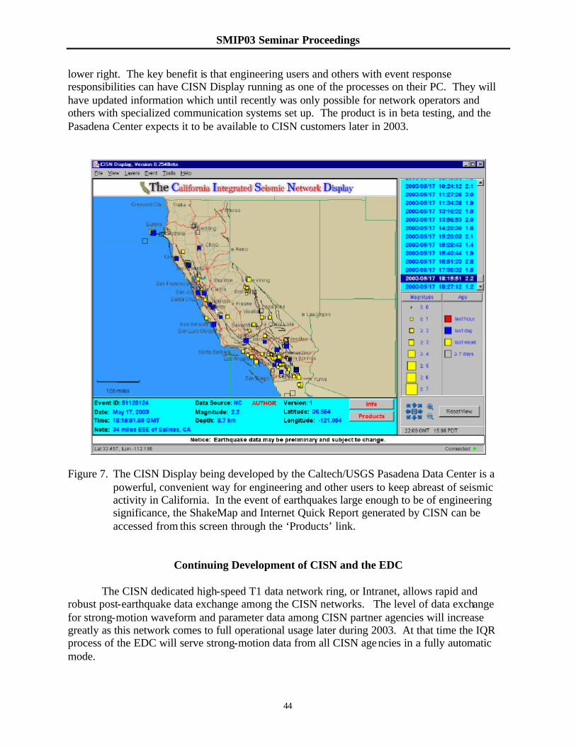
SMIP03 Seminar Proceedings
44
lower right. The key benefit is that engineering users and others with event response responsibilities can have CISN Display running as one of the processes on their PC. They will have updated information which until recently was only possible for network operators and others with specialized communication systems set up. The product is in beta testing, and the Pasadena Center expects it to be available to CISN customers later in 2003.
Figure 7. The CISN Display being developed by the Caltech/USGS Pasadena Data Center is a powerful, convenient way for engineering and other users to keep abreast of seismic activity in California. In the event of earthquakes large enough to be of engineering significance, the ShakeMap and Internet Quick Report generated by CISN can be accessed from this screen through the ‘Products’ link.
Continuing Development of CISN and the EDC
The CISN dedicated high-speed T1 data network ring, or Intranet, allows rapid and robust post-earthquake data exchange among the CISN networks. The level of data exchange for strong-motion waveform and parameter data among CISN partner agencies will increase greatly as this network comes to full operational usage later during 2003. At that time the IQR process of the EDC will serve strong-motion data from all CISN agencies in a fully automatic mode.

SMIP03 Seminar Proceedings
45
CISN is one region of the nationwide Advanced National Seismic System. The tools and techniques developed for the CISN Engineering Data Center, in the most seismically active region in the ANSS, may be similarly employed, with local adjustments, in other regions with less frequent, though very similar, needs for engineering information after significant earthquake shaking.
Summary The CISN Engineering Data Center greatly accelerates access to data after earthquakes
and allows users to conveniently obtain data for specific structures and structure types. The development of the EDC is continuing and will focus on the following areas:
• Fully automating the Internet Quick Report, to be available routinely within 15 minutes or less after M>4 earthquakes by later in 2003; until then it is partly manual and will be available within minutes to hours after a significant earthquake.
• Continuing to expand the search capability, to allow users to conveniently access strong-
motion earthquake data and detailed information on instrumented structures and other stations, including location, site geology, structural system, sensor layouts, and other information. The data archives are being populated to include strong-motion data and station/structure information from previous earthquakes, from the CSMIP and NSMP networks and the other partners.
• Expanding the linking between the Internet Quick Report and the ShakeMap for an
earthquake, allowing users to see the regional and the very local shaking associated with an earthquake, in forms customarily used in earthquake engineering.
References Ambraseys, N., P. Smit, R. Sigbjörnsson, P. Suhadolc, and B. Margaris (2002). Internet Site for
European Strong-Motion Data, EVR1-CT-1999-40008, European Commission, Directorate-General XII, Environmental and Climate Programme, Bruxelles, Belgium; Internet address: http://www.isesd.cv.ic.ac.uk/.
Archuleta, R. (2000). COSMOS Virtual Data Center, in Proceedings SMIP2000 Seminar on
Utilization of Strong-Motion Data, p. 97-114. CSMIP (1994). First Quick Report on CSMIP Strong-motion Data from the San Fernando
Valley Earthquake of January 17, 1994, OSMS Report 94-01, 10 pp., 17 January 1994. Kircher, C.A. (2003). Near-Real-Time Loss Estimation Using HAZUS and ShakeMap Data, in
Proceedings SMIP03 Seminar on Utilization of Strong-Motion Data.

SMIP03 Seminar Proceedings
46
Lin, Kuo-Wan, A.F. Shakal and C. Stephens (2001). TriNet/CISN Engineering Strong Motion Data Center and the Internet Quick Report, in Proceedings SMIP01 Seminar on Utilization of Strong-Motion Data, p. 53-64.
Lin, Kuo-Wan, A.F. Shakal, M. Huang, C. Stephens and W. Savage (2002). Dissemination of
Strong Motion via the Internet Quick Report and the Internet Data Report at the CISN Engineering Data Center, in Proceedings SMIP02 Seminar on Utilization of Strong-Motion Data, p. 115-126.
Porcella, R.L., E.C. Etheridge, R.P. Maley and A.V. Acosta (1994). Accelerograms recorded at USGS National Strong-Motion Network stations during the Ms 6.6 Northridge, California earthquake of January 17, 1994, USGS OFR 94-141, 100 pp.
Rojahn, C., C.D. Comartin and S.A. King (2003). Guidelines for Utilizing Strong-Motion and ShakeMap Data in Post-Earthquake Response (ATC-54), in SMIP03 Seminar on Utilization of Strong-Motion Data.
Shakal, A., M. Huang, R. Darragh, T. Cao, R. Sherburne, P. Malhotra, C. Cramer, R. Sydnor, V. Graizer, G. Maldonado, C. Petersen and J. Wampole (1994). CSMIP strong motion records from the Northridge, California earthquake of 17 January 1994, Report OSMS 94-07, 308 pp.
Shakal, A.F. and C.F. Scrivner (2000). TriNet Engineering Strong-Motion Data Center, in Proceedings SMIP2000 Seminar on Utilization of Strong-Motion Data, p. 115-124.
Wald, D.J., V. Quitoriano, T. Heaton, C.F. Scrivner and C. Worden (1999). TriNet ShakeMaps: Rapid Generation of Instrumental Ground Motion and Intensity Maps for Earthquakes in Southern California, Earthquake Spectra, 15, 537-556.
SMIP03 Seminar Proceedings
47
GUIDELINES FOR UTILIZING STRONG-MOTION AND SHAKEMAP DATA IN POST-EARTHQUAKE RESPONSE (ATC-54)
Christopher Rojahn
Craig D. Comartin Stephanie A. King
Applied Technology Council Comartin-Reis Weidlinger Associates Redwood City, California Sacramento, California Los Altos, California
Abstract
The ATC-54 Report, Guidelines for Utilizing Strong-Motion Data and ShakeMaps in Post-earthquake Response, prepared by the Applied Technology Council for the California Geological Survey, provides guidance on (1) the use of near-real-time computer-generated ground-motion maps in emergency response, and (2) the use and interpretation of strong-motion data to evaluate the earthquake response of buildings, bridges, and dams in the immediate postearthquake aftermath. Guidance is also provided on the collection of data describing the characteristics and performance of structures in which, or near which, strong-motion data have been recorded.
Introduction
Background
Since the installation of the initial network of nine strong-motion instruments at ground sites and in buildings in California in 1932 (Matthiesen, 1980), the number of strong-motion recording stations and records has grown dramatically. Today there are more than 1000 instrumented sites and structures in California, including buildings, dams, bridges, and other lifeline structures. The instruments are operated by a wide variety of agencies and owners, including the California Geological Survey (CGS), California Division of Water Resources, California Department of Transportation, U.S. Geological Survey (USGS), U.S. Bureau of Reclamation, U.S. Army Corp of Engineers, several universities and university-affiliated centers, utility companies in northern and southern California, and owners of buildings where instruments have been mandated by building code requirements. Hundreds of strong-motion time histories have been recorded at these stations, resulting primarily from large damaging earthquakes, such as the 1971 San Fernando, 1989 Loma Prieta, and 1994 Northridge earthquakes. Such data are available in digital form from the principal network operators (CGS and the USGS) and other sources, including the world wide web virtual data center operated by the Consortium of Organizations for Strong-Motion Observation Systems (COSMOS).
Over the last 40 to 50 years, the technology for recording, analyzing, and representing
strong-motion data has also advanced significantly. Major advances have included: the development of rapid scanning and processing techniques for converting photographic analog records to digital format; the development and deployment of digital accelerographs; the

SMIP03 Seminar Proceedings
48
development of new computer analytical methods that use strong-motion records to verify and refine computer models of structural response and to compute estimated component forces and displacements; and, most recently, the introduction of computer-generated ground-motion maps that provide estimates of the regional distribution of ground shaking within minutes, and without human intervention, after damaging earthquakes.
Collectively the existing network of strong-motion instruments, the existing sets of strong-
motion data, and the available techniques and technology for processing, analyzing, and displaying strong-motion data provide an ideal set of tools and information for postearthquake response planning and execution, as well as postearthquake evaluation of structures. In recognition of the enormous potential of these tools and information, and with the realization that practicing professionals do not have guidance readily available on how to take advantage of these current technical capabilities, CGS awarded a Year 2000 California Strong-Motion Instrumentation Program (CSMIP) Data Interpretation Project to the Applied Technology Council (ATC) to prepare the needed guidance. Specifically, the contract required that ATC develop Guidelines to: (1) facilitate improved emergency response with the use of near-real-time computer-generated ground-motion maps and; (2) facilitate postearthquake evaluation of structures using strong-motion data from ground sites and instrumented buildings, bridges, and dams. Under this project ATC also provided guidance on the collection of data describing the characteristics and performance of structures in which, or near which, strong-motion data have been recorded.
Guidelines Development Process
The ATC-54 Guidelines were developed through a multi-step approach by a multi-disciplinary team of experienced specialists in earthquake and geotechnical engineering, risk analysis, geographic information systems (GIS), and emergency response planning. Initially, the project team identified and described the state-of-the-art in available data resources, building and lifeline inventory data, GIS hazard maps, and loss estimation tools. The next step was to define the state-of-the-practice in emergency response planning at the state, regional, and local level, as well as in postearthquake structural surveys and evaluations. Based on this information, primarily developed through literature reviews and interviews with key individuals in various agencies and organizations throughout the state, an assessment was made of the existing capabilities in emergency response planning and postearthquake evaluation of structures. This assessment served as the basis for determining the level of information and extent of guidance to be provided in the Guidelines. The Guidelines development process also included a Users’ Workshop organized to solicit input on the content and scope of the Guidelines. The finalized version of the Guidelines is based on input received at the Users’ Workshop, as well as review comments from the CSMIP staff and the California Seismic Safety Commission’s Strong-Motion Instrumentation Advisory Committee (SMIAC).
Paper Focus and Contents
This paper is seventh in a series of papers initially presented in the SMIP01 Seminar (Brady and Rojahn, 2001; King, Comartin, Reis, Nathe, and Power, 2001; Rojahn, Comartin, and King, 2001) and subsequently in the SMIP02 Seminar (King, Comartin, Reis, Nathe, and Power, 2002;
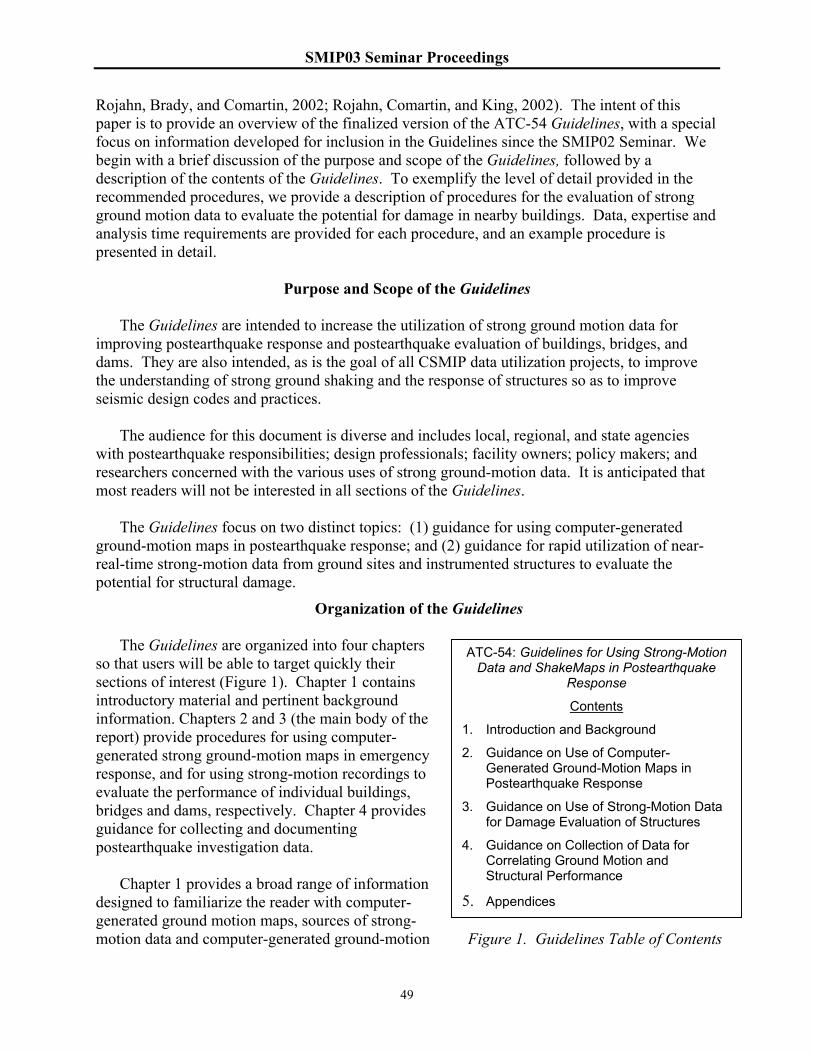
SMIP03 Seminar Proceedings
49
Rojahn, Brady, and Comartin, 2002; Rojahn, Comartin, and King, 2002). The intent of this paper is to provide an overview of the finalized version of the ATC-54 Guidelines, with a special focus on information developed for inclusion in the Guidelines since the SMIP02 Seminar. We begin with a brief discussion of the purpose and scope of the Guidelines, followed by a description of the contents of the Guidelines. To exemplify the level of detail provided in the recommended procedures, we provide a description of procedures for the evaluation of strong ground motion data to evaluate the potential for damage in nearby buildings. Data, expertise and analysis time requirements are provided for each procedure, and an example procedure is presented in detail.
Purpose and Scope of the Guidelines
The Guidelines are intended to increase the utilization of strong ground motion data for
improving postearthquake response and postearthquake evaluation of buildings, bridges, and dams. They are also intended, as is the goal of all CSMIP data utilization projects, to improve the understanding of strong ground shaking and the response of structures so as to improve seismic design codes and practices.
The audience for this document is diverse and includes local, regional, and state agencies
with postearthquake responsibilities; design professionals; facility owners; policy makers; and researchers concerned with the various uses of strong ground-motion data. It is anticipated that most readers will not be interested in all sections of the Guidelines.
The Guidelines focus on two distinct topics: (1) guidance for using computer-generated
ground-motion maps in postearthquake response; and (2) guidance for rapid utilization of near-real-time strong-motion data from ground sites and instrumented structures to evaluate the potential for structural damage.
Organization of the Guidelines The Guidelines are organized into four chapters
so that users will be able to target quickly their sections of interest (Figure 1). Chapter 1 contains introductory material and pertinent background information. Chapters 2 and 3 (the main body of the report) provide procedures for using computer-generated strong ground-motion maps in emergency response, and for using strong-motion recordings to evaluate the performance of individual buildings, bridges and dams, respectively. Chapter 4 provides guidance for collecting and documenting postearthquake investigation data.
Chapter 1 provides a broad range of information
designed to familiarize the reader with computer-generated ground motion maps, sources of strong-motion data and computer-generated ground-motion
ATC-54: Guidelines for Using Strong-Motion Data and ShakeMaps in Postearthquake
Response
Contents
1. Introduction and Background
2. Guidance on Use of Computer-Generated Ground-Motion Maps in Postearthquake Response
3. Guidance on Use of Strong-Motion Data for Damage Evaluation of Structures
4. Guidance on Collection of Data for Correlating Ground Motion and Structural Performance
5. Appendices
Figure 1. Guidelines Table of Contents

SMIP03 Seminar Proceedings
50
maps (including current web site addresses of principal providers). Chapter 1 also introduces current strategic planning for seismic monitoring statewide, including the goals for the next five years of the California Integrated Seismic Network1 (CISN). The discussion notes that as efforts are undertaken in coming years to meet these goals, as well as the goals of the proposed Advanced National Seismic System2 (ANSS), the overview of strong-motion data resources in California provided in Chapter 1 is certain to be superceded by more current information. In general, it is noted that the efforts under the CISN and ANSS will provide additional resources and programs that will undoubtedly result in the more effective implementation of the Guidelines.
Chapter 2 covers procedures for
using computer-generated maps for postearthquake response (see example in Figure 2). Such maps, known as ShakeMaps, are generated automatically following moderate and large earthquakes and are normally posted within several minutes of the earthquake origin time, without the aid of human-kind. These maps show the distribution of peak ground acceleration and velocity, spectral acceleration at three periods, and an instrumentally-derived, estimated distribution of Instrumental Intensity, which is akin to Modified Mercalli Intensity. Instrumental Intensity maps are based on a combined regression of recorded peak acceleration and velocity amplitudes. Chapter 2 begins with a section on the general framework for the use of real-time ShakeMap data for emergency response, including the data resources and procedures that are
1 The California Integrated Seismic Network is being proposed to provide the organizational framework to integrate the existing, separate monitoring networks in California into a single seismic monitoring system. The CISN Draft Strategic Plan for 2002-2006 includes the following goals: (1) operate a reliable and robust statewide system to record earthquake ground motions over the relevant range of frequencies and shaking levels; (2) distribute information about earthquakes rapidly after their occurrence for emergency response and public information; (3) create an easily accessible archive of California earthquake data for engineering and seismological research, including waveform data and derived products; (4) maintain CISN infrastructure as a reliable state-of-the-art data collection, processing, and information distribution system; (5) apply the latest research and technology to develop new algorithms for analyzing earthquake data and extracting more detailed information for new user products; and (6) maximize the use and benefit of real-time seismic information and other rapidly evolving tools and technologies through technology transfer to the user community. 2 The Advanced National Seismic System Network, as currently planned, will be a nationwide network of at least 7,000 shaking measurement systems, both on the ground and in buildings (USGS, 2000).
Figure 2. TriNet ShakeMap for the 1994 Northridge, California earthquake (USGS, 2000).
SMIP03 Seminar Proceedings
51
commonly related to the utilization of strong ground motion data for the various areas of emergency response. The subsequent sections provide guidance (with illustrative examples) on the development and implementation of applications using ShakeMaps for emergency response. The following applications are addressed:
• extent of damaged buildings and planning related safety evaluation inspections;
• condition of hospitals and other emergency response structures;
• impact on utility systems and transportation networks;
• extent of liquefaction, landslide, and inundation;
• casualties and associated need for victim extraction from damaged structures;
• extent of debris from collapsed structures;
• sheltering needs;
• extent of possible hazardous materials release;
• estimates of economic losses; and
• insurance claims.
Chapter 3 provides guidance for interpretation of strong-motion data in the immediate earthquake aftermath (within minutes to days after the earthquake) to evaluate structural performance. Specific procedures are provided for evaluation of strong-motion data in or near buildings and more general guidance on instrumentation and performance assessment is provided for bridges and dams. In general the procedures apply to records of acceleration recorded as a function of time, otherwise known as acceleration time histories, or accelerograms. Extensive background information is also provided, including discussions of (1) prior efforts to evaluate strong-mootion to assess structural performance; (2) the limitations of data from instrumented structures; (3) existing strong-motion networks; and (4) data sources and processing. The main focus of the chapter is a set of procedures for the evaluation of strong-motion data recorded in or near buildings. One set of procedures pertain to the evaluation of ground motion data to determine the likelihood of potential damage in nearby structures. These procedures enable:
• comparisons of ground motions estimated from ShakeMaps with design ground motions (PROCEDURE 1);
• comparisons of recorded ground motions with design ground motions (PROCEDURE 2); and
• estimation of building drift ratios and their significance in terms of damage potential (PROCEDURE 3).
A second set of procedures pertain to the evaluation of strong-motion from instrumented buildings. These procedures include:
• visual examination techniques to (1) identify changes in modal periods of response and estimate mode shapes, story forces, story shears, and overturning moments (PROCEDURE 4); and (2) evaluate high-frequency bursts of acceleration (PROCEDURE 5);
SMIP03 Seminar Proceedings
52
• Fast Fourier Transform moving-window analysis to evaluate changes in building period (PROCEDURE 6);
• displacement time history analysis to estimate building periods, inter-story drift, in-plane bending response, and torsional response (PROCEDURE 7);
• an approach to develop push-over curves using data from more than one earthquake (PROCEDURE 8); and
• system identification techniques to define and verify mathematical computer models of building behavior (PROCEDURE 9).
The description of each procedure includes (1) expertise and time required to execute the procedure; (2) applicable structural framing systems, (3) instrumentation and data required, (4) steps to be taken, and (5) example applications. In certain instances, the procedures applicable to buildings are also applicable to the evaluation of strong-motion data from instrumented bridge and dam sites. The applicability of these procedures is described in those sections of Chapter 3 pertaining to bridges and dams.
Chapter 4 focuses on procedures for documenting structural attributes and performance in the
vicinity of ground motion recordings. Similar to Chapter 3, this chapter covers procedures for buildings, bridges, and dams and provides guidance for both instrumented and non-instrumented structures. For non-instrumented buildings, the procedures draw heavily on the approach used after the 1994 Northridge earthquake to collect data on the characteristics and performance of more than 500 buildings within 1000 feet of strong-motion recording sites. For each structure type, the steps for data collection, data formatting and archiving, and data analysis and dissemination are included.
Seven appendices are included that contain supplemental information. Appendix A describes
the process that was used to develop this document. Appendix B includes a summary of the most commonly used regional earthquake loss-estimation methods, which are referenced in Chapter 2. Appendix C provides guidance on strong-motion instrumentation of buildings, and Appendix D contains a summary of the most commonly used linear and nonlinear structural analysis software programs. Appendix E provides guidance on strong-motion instrumentation of bridges (with examples instrumented by the California Department of Transportation), and Appendix F provides resources and guidance for strong-motion instrumentation of dams. Postearthquake survey forms are provided in Appendix G.
Procedures for Evaluation of Building Damage Potential
Using Strong Ground Motion Data This set of procedures pertains to the evaluation of recorded or estimated strong ground
motion data to determine the likelihood of potential damage to a building or nearby buildings. Data recorded in the upper stories of the building are not used in this set of procedures. The first procedure (PROCEDURE 1, see the following text) uses information from ShakeMaps (described in Chapter 2) to prepare estimated acceleration response spectra for the site(s) under

SMIP03 Seminar Proceedings
53
consideration. The remaining procedures3,4 use strong-motion data recorded at the ground or basement level of the building, or at a nearby free-field site. For each procedure, information is provided on (1) expertise and time required to execute the procedure; (2) applicable structural framing systems and data required, (3) steps to be taken, and (4) example applications. The requirements for the various procedures that use estimated or recorded ground motion are summarized in Table 1. This table also provides estimates of the uncertainty in the results.
Table 1. Matrix of Requirements for Procedures Using Ground Motion Information and Associated Uncertainty in the Results
Procedure Data Required
Level of Expertise Required
Execution Time (Estimated)
Applicable Building Types
Uncertainty in Results
PROCEDURE 1: Comparison of acceleration response spectra computed from ShakeMap data with design lateral-force coefficient
ShakeMap estimates of peak ground acceleration and spectral acceleration response at 0.3 and 1 second; design lateral-force coefficient
Engineering analyst; ability to compute response spectra from ShakeMap data
Minutes to Hours
Low-rise and mid-rise concrete-wall* and masonry-wall buildings (up to 7 stories in height)
High
PROCEDURE 2: Comparison of acceleration response spectra computed for recorded horizontal ground motions with design lateral-force coefficient
Strong-motion record from basement, ground level, or nearby free-field site; design lateral-force coefficient
Engineering analyst
Hours to Days
Low-rise and mid-rise concrete-wall* and masonry-wall buildings (up to 7 stories in height)
Moderate
PROCEDURE 3: Estimation of roof drift ratio using displacement response spectra computed for recorded horizontal ground motions
Strong-motion record from basement, ground level, or nearby free-field site; building height, in feet
Engineering analyst
Hours to Days
Wood-frame, concrete-frame, and steel-frame buildings up to 12 stories in height)
Moderate
*Includes tilt-up buildings
PROCEDURE 1: Comparison of Shakemap-Derived Response Spectra with Seismic Design Coefficient
This procedure compares acceleration response spectra estimated from ShakeMap ordinates of spectral response to design lateral-force coefficients to evaluate whether the ground motions
3 PROCEDURE 2: Comparison of Acceleration Response Spectra Computed for Recorded Horizontal Ground Motions With Design Lateral-Force Coefficient 4 PROCEDURE 3: Estimation of Roof Drift Ratio Using Displacement Response Spectra Computed for Recorded Horizontal Ground Motions

SMIP03 Seminar Proceedings
54
that occurred at the base of a building exceeded those associated with the lateral-force coefficient used in design.
Expertise and Time Required. This procedure requires the ability to (1) interpret ShakeMaps that provide spectral ordinates for 0.3 second and 1.0 second periods; (2) compute response spectra using this information; and (3) estimate the lateral-force coefficient for the building under consideration. This requires a level of expertise normally attributable to an engineering analyst (Professional Engineer), with an ability to use MapInfo or equivalent geographic information system (GIS) software.
The procedure can be executed in minutes to hours, assuming the person executing the procedure has the necessary expertise.
Applicability and Required Data. This procedure applies to stiff, low-rise and mid-rise buildings (up to seven stories), such as masonry-wall, concrete shear-wall, and tilt-up buildings. The procedure requires the computation of acceleration response spectra using spectral ordinates of horizontal motions taken from ShakeMaps. The procedure also requires an estimate of the lateral-force coefficient used in design.
Steps. The procedure consists of the following steps:
1. For the main shock under consideration, download the following maps from the ShakeMap website (www.trinet.org): (1) map showing contours of peak ground acceleration (PGA); (2) map showing contours of pseudo acceleration response for 0.3 sec period (Sa,0.3); and (3) map showing contours of pseudo acceleration response for 1.0 second period (Sa,1). Transfer electronic versions of the maps to MapInfo, or equivalent. Locate the building site on each contour map. Determine the value of PGA, Sa,0.3, and Sa,1 for the site. Construct an acceleration response spectrum for 5% effective damping, based on the following: (1) Sa,0 is the PGA value; (2) Sa,0.3 defines the level of the plateau that will span from To to Ts; (3) Ts for 5% damping is given by Sa,1 / Sa,0 (see FEMA 356, Equation 1-11); (4) To is given by 0.2 Ts (see FEMA 356, Equation 1-12); and (5) the acceleration decreases as 1/T from the right-hand end of the plateau, passing through the map value for T = 1 sec.
2. Estimate the fundamental period, T (seconds), of the building under consideration, using the following equation: T = 0.025h0.75, where h (ft) is the height of the building. The equation is based on the period equation given in FEMA-356 (ASCE, 2000) for “other” buildings; the multiplier of 0.025, however, has been increased from 0.02 (an increase of 25%) to account for the conservative nature of the FEMA 356 equation, which is recognized in the FEMA 356 commentary section as under estimating periods during strong ground shaking.
3. Calculate the average acceleration response in the period range, 0.8T to 1.2T, where T is the fundamental period of vibration. (Averaging the spectra over a range of periods close to the estimated fundamental period of the building is recommended, to smooth the peaks and valleys inherent in acceleration response spectra.)
4. Determine the lateral-force coefficient, defined as the design lateral force divided by the building weight, by referring to the original design calculations, if available, or by determining the design date and referring to the design lateral-force equation in the code that likely was used in the design process. For a multistory building, only a fraction of the building weight is considered to participate in the first mode response. This factor is called
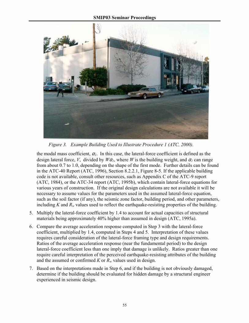
SMIP03 Seminar Proceedings
55
the modal mass coefficient, α1. In this case, the lateral-force coefficient is defined as the design lateral force, V, divided by Wα1, where W is the building weight, and α1 can range from about 0.7 to 1.0, depending on the shape of the first mode. Further details can be found in the ATC-40 Report (ATC, 1996), Section 8.2.2.1, Figure 8-5. If the applicable building code is not available, consult other resources, such as Appendix C of the ATC-9 report (ATC, 1984), or the ATC-34 report (ATC, 1995b), which contain lateral-force equations for various years of construction. If the original design calculations are not available it will be necessary to assume values for the parameters used in the assumed lateral-force equation, such as the soil factor (if any), the seismic zone factor, building period, and other parameters, including K and Rw values used to reflect the earthquake-resisting properties of the building.
5. Multiply the lateral-force coefficient by 1.4 to account for actual capacities of structural materials being approximately 40% higher than assumed in design (ATC, 1995a).
6. Compare the average acceleration response computed in Step 3 with the lateral-force coefficient, multiplied by 1.4, computed in Steps 4 and 5. Interpretation of these values requires careful consideration of the lateral-force framing type and design requirements. Ratios of the average acceleration response (near the fundamental period) to the design lateral-force coefficient less than one imply that damage is unlikely. Ratios greater than one require careful interpretation of the perceived earthquake-resisting attributes of the building and the assumed or confirmed K or Rw values used in design.
7. Based on the interpretations made in Step 6, and if the building is not obviously damaged, determine if the building should be evaluated for hidden damage by a structural engineer experienced in seismic design.
Figure 3. Example Building Used to Illustrate Procedure 1 (ATC, 2000).

SMIP03 Seminar Proceedings
56
Example. The building in this example is a tilt-up building located in the San Fernando Valley (see Figure 3), designed in 1978 and constructed in 1979 (location and design and construction dates selected for this example are hypothetical). The building was strongly shaken by the 1994 Northridge earthquake and no damage to the exterior was observed by the postearthquake safety assessment team that inspected the building a day after the main shock. Since the team does not have access to the interior or the roof of the building, they are interested in reviewing quantitative information on strong shaking that would assist them in determining likelihood of hidden damage. The ideal characterization would be a plot of acceleration spectral response.
In Step 1 ShakeMaps showing contours of PGA, Sa,0.3, and Sa,1 were downloaded from the TriNext web site (Figure 4a,b,c) using wireless technology and a lap top computer. Through the use of MapInfo the assessment team was able to determine the following ground motion parameters for the site: PGA, 0.37g; Sa,0.3, 1.1 g; Sa,1, 0.56 g. Based on these values and using the instructions of Step 1, the response spectrum shown in Figure 5 was constructed in a Microsoft Excel spread sheet.
In Step 2, the period of the example building was determined using the default formula for "other buildings", and assuming the story height is 18 ft, as follows:
T=0.025 h 0.75 = 0.025 × (18) 0. 75 = 0.22 sec.
(a) PGA contours
(b) Pseudo acceleration response at
(c) Pseudo acceleration response atFigure 4. ShakeMaps for 1994
Northridge earthquake showing location of example building (star).
0
0.2
0.4
0.6
0.8
1
1.2
0 0.5 1 1.5 2
Period (sec.)
Spec
tral A
ccele
ration
(g)
Figure 5. Acceleration response spectrum for example building created from ShakeMap data.
SMIP03 Seminar Proceedings
57
The average amplitudes of acceleration response in the period range from 0.18 to 0.26 sec (0.8T to 1.2T range) were calculated in Step 3 using acceleration response values from the Excel spread sheet. The average of these amplitudes is 1.1 g.
In Step 4, the lateral-force coefficient was estimated to be 0.186, based on the team’s knowledge of construction practices in the area and the formula for calculating base shear in the 1976 Uniform Building Code. Divided this amount by the modal mass coefficient, which is assumed to be 1.0, and multiplying the result by 1.4 in Step 5 yielded an assumed effective lateral-force coefficient of 0.26.
Finally, in Step 6, a comparison of the average acceleration response for periods close to the calculated fundamental period of the building (0.22 second) with the assumed lateral-force coefficient (from Step 5) indicated that the average acceleration response, based on recorded motions at the site, was 1.1/0.26 = 4.2 times higher than the assumed lateral-force coefficient. Given the high earthquake accelerations, relative to the design coefficient, the postearthquake safety assessment team gained access to the building and determined that there was insignificant structural damage. The building was subsequently posted per the ATC-20 procedures (ATC, 1989, 1995) as INSPECTED (apparently safe based on an interior and exterior inspection).
Concluding Remarks
The ATC-54 Guidelines document is envisioned as a living document, with periodic updates and revisions as new knowledge, information, and technologies become available. The Applied Technology Council and the Strong-Motion Instrumentation Program of the California Geological Survey intend that the document remain as a primary resource for guidance on the use of computer-generated ShakeMaps in emergency response and for guidance on state-of-the-art procedures for rapid evaluation of structures using strong-motion data. Suggestions for improvement are encouraged.
References
ATC, 1984, An Evaluation of the Imperial County Services Building Earthquake Response and
Associated Damage, ATC-9 Report, Applied Technology Council, Redwood City, California, 231 pages.
ATC, 1995a, Structural Response Modification Factors, ATC-19 Report, Applied Technology Council, Redwood City, California, 70 pages.
ATC, 1995b, A Critical Review of Current Approaches to Earthquake Resistant, ATC-34 Report, Applied Technology Council, Redwood City, California, 94 pages.
ATC, 1996, Sesimic Evaluation and Retrofit of Concrete Buildings, ATC-40 Report, Applied Technology Council, Redwood City, California, 626 pages.
ATC, 2003, Guidelines for Utilizing Strong-Motion and ShakeMap Data in Postearthquake Response, ATC-54 Report, Applied Technology Council, Redwood City, California.
Brady, A. G., and Rojahn, Christopher, 2001, "Guidelines for utilizing strong-motion data for evaluation of structures ", SMIP01 Seminar on Seismological and Engineering Implications

SMIP03 Seminar Proceedings
58
of Recent Strong-Motion Data, Los Angeles, Sep 12, 2001, California Division of Mines and Geology, Sacramento.
King, S.A., Comartin, C.D., Reis, Evan, Nathe, S.K., and Power, M.S., 2001, Guidelines for utilizing ShakeMaps for emergency response, Proceedings, SMIP01 Seminar on Seismological and Engineering Implications of Recent Strong-Motion Data, Los Angeles, California, California Division of Mines and Geology, Sacramento.
King, S.A., Comartin, C.D., Reis, Evan, Nathe, S.K., and Power, M.S., 2002, Guidelines for utilizing ShakeMaps for emergency response, Proceedings, SMIP02 Seminar on Utilization of Strong-Motion Data, Los Angeles, California Geological Survey, Sacramento, California.
Matthiesen, R.B., 1980, “Building Instrumentation Programs,” in Proceedings, Workshop on Interpretation of Strong-Motion Earthquake Records in and/or Near Buildings, UCLA Report No. 8015, University of California at Los Angeles, Los Angeles, California.
Rojahn, Christopher, Brady, A. G., and Comartin, C.D., 2002, “Guidelines for utilizing strong-motion for postearthquake evaluation of structures,” Proceedings, SMIP02 Seminar on Utilization of Strong-Motion Data, Los Angeles, California Geological Survey, Sacramento, California.
Rojahn, Christopher, Comartin, C.D., and King, S.A., 2001, "Guidelines for utilizing strong-motion and ShakeMap data in postearthquake response: an overview", Proceedings, SMIP01 Seminar on Seismological and Engineering Implications of Recent Strong-Motion Data, Los Angeles, California Division of Mines and Geology, Sacramento.
Rojahn, Christopher, Comartin, C.D., and King, S.A., 2002, “Guidelines for utilizing strong-motion and ShakeMap data in postearthquake response: an overview,” Proceedings, SMIP02 Seminar on Utilization of Strong-Motion Data, Los Angeles, California Geological Survey, Sacramento, California.
USGS, 2000, ANSS-Advanced National Seismic System, U. S. Geological Survey Fact Sheet 075-00, Reston, Virginia.
Acknowledgments The authors gratefully acknowledge Gerald Brady, Sarah Nathe, Maurice Power, and Evan
Reis, who gathered data and summarized the state-of-the-art and state-of-the-practice, and the Project Resource and Advisory Group, who provided guidance on various aspects of the project: Thalia Anagnos, Mehmet Celebi, Lloyd Cluff, Charles Eadie, Sigmund Freeman, Terry Haney, Anne Kiremidjian, Ronald Mayes, Andrew Merovich, Lawrence Reaveley, James Russell, and Chris Tokas.

SMIP03 Seminar Proceedings
59
NEAR-REAL-TIME LOSS ESTIMATION USING HAZUS AND SHAKEMAP DATA
Charles A. Kircher, Ph.D., P.E.
Kircher & Associates 1121 San Antonio Road, Suite D-202
Palo Alto, California 94303
Introduction
This paper describes real-time damage and loss estimation using the HAZUS earthquake loss estimation technology and ShakeMap data, and provides an example comparison of predicted and observed losses for the 1994 Northridge earthquake.
HAZUS [NIBS, 1999, Kircher et al., 1997a/1997b, Whitman et al., 1997] is the standardized
earthquake loss estimation methodology developed by the National Institute of Building Sciences (NIBS) for the United States Federal Emergency Management Agency (FEMA). HAZUS was originally developed to assist emergency response planners to "provide local, state and regional officials with the tools necessary to plan and stimulate efforts to reduce risk from earthquakes and to prepare for emergency response and recovery from an earthquake."
HAZUS can also be used to make regional estimates of damage and loss following and
earthquake using ground motion, ShakeMap, data provided by the United States Geological Survey (USGS) as part of Tri-Net in Southern California [Wald et al., 1999] or by other regional strong-motion instrumentation networks.
ShakeMaps
ShakeMaps are produced immediately following an earthquake in California (and certain
other high-seismic regions of the US) and made available via the Internet. ShakeMaps are based on instrumental measurements of ground shaking (when instrumental records are available) and provide a more accurate and certain description of seismic demand. Since even the most extensive set of strong-motion instruments is still less than one station per census tract, on average, ShakeMaps have limited accuracy at the census tract, or smaller area, level. Nonetheless, they are an improvement over estimates of ground shaking based solely on predictive (magnitude-distance) equations that do not capture actual patterns and trends in the propagation of seismic waves.
Figure 1 is a ShakeMap of instrumental intensity for the 1994 Northridge earthquake
showing, qualitatively, areas of stronger and weaker ground shaking. This map is a useful tool for rapidly identifying areas that would be expected to be hardest hit by the earthquake (e.g., areas shown in shown in orange and red), but does not provide quantitative estimates of damage and loss (in terms of economic impacts, casualties, etc.). HAZUS may be used to transform the qualitative information of ShakeMaps into quantitative estimates of damage and loss.

SMIP03 Seminar Proceedings
60
Figure 1. ShakeMap of instrumental intensity of the 1994 Northridge earthquake.
Comparison of Losses – 1994 Northridge Earthquake
Figure 2 shows the large HAZUS study region used to estimate losses for the 1994 Northridge earthquake that includes all 1,652 census tracts of Los Angeles County, and 743 census tracts of affected areas of neighboring counties.
Figure 2. 1994 Northridge earthquake study region.
Boundary Extent for Somerville's Data
Boundary Extent for ShakeMap Data
0 50
kilometers
RiversideRiversideRiversideRiversideRiversideRiversideRiversideRiversideRiverside
San BernardinoSan BernardinoSan BernardinoSan BernardinoSan BernardinoSan BernardinoSan BernardinoSan BernardinoSan Bernardino
Los AngelesLos AngelesLos AngelesLos AngelesLos AngelesLos AngelesLos AngelesLos AngelesLos AngelesSanta BarbaraSanta BarbaraSanta BarbaraSanta BarbaraSanta BarbaraSanta BarbaraSanta BarbaraSanta BarbaraSanta Barbara
San DiegoSan DiegoSan DiegoSan DiegoSan DiegoSan DiegoSan DiegoSan DiegoSan Diego
OrangeOrangeOrangeOrangeOrangeOrangeOrangeOrangeOrange
KernKernKernKernKernKernKernKernKern
spospospospospospospospospo
VenturaVenturaVenturaVenturaVenturaVenturaVenturaVenturaVentura
MMI 9MMI 8MMI 7MMI 6MMI 5
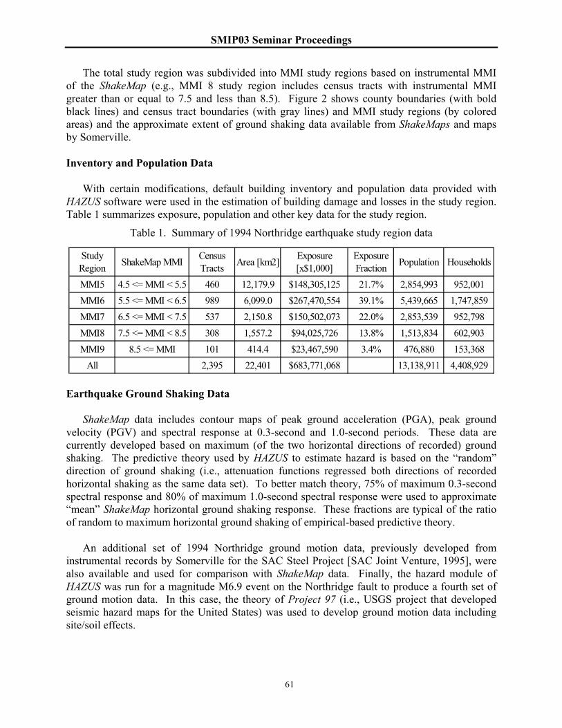
SMIP03 Seminar Proceedings
61
The total study region was subdivided into MMI study regions based on instrumental MMI of the ShakeMap (e.g., MMI 8 study region includes census tracts with instrumental MMI greater than or equal to 7.5 and less than 8.5). Figure 2 shows county boundaries (with bold black lines) and census tract boundaries (with gray lines) and MMI study regions (by colored areas) and the approximate extent of ground shaking data available from ShakeMaps and maps by Somerville.
Inventory and Population Data
With certain modifications, default building inventory and population data provided with HAZUS software were used in the estimation of building damage and losses in the study region. Table 1 summarizes exposure, population and other key data for the study region.
Table 1. Summary of 1994 Northridge earthquake study region data
Earthquake Ground Shaking Data
ShakeMap data includes contour maps of peak ground acceleration (PGA), peak ground velocity (PGV) and spectral response at 0.3-second and 1.0-second periods. These data are currently developed based on maximum (of the two horizontal directions of recorded) ground shaking. The predictive theory used by HAZUS to estimate hazard is based on the “random” direction of ground shaking (i.e., attenuation functions regressed both directions of recorded horizontal shaking as the same data set). To better match theory, 75% of maximum 0.3-second spectral response and 80% of maximum 1.0-second spectral response were used to approximate “mean” ShakeMap horizontal ground shaking response. These fractions are typical of the ratio of random to maximum horizontal ground shaking of empirical-based predictive theory.
An additional set of 1994 Northridge ground motion data, previously developed from
instrumental records by Somerville for the SAC Steel Project [SAC Joint Venture, 1995], were also available and used for comparison with ShakeMap data. Finally, the hazard module of HAZUS was run for a magnitude M6.9 event on the Northridge fault to produce a fourth set of ground motion data. In this case, the theory of Project 97 (i.e., USGS project that developed seismic hazard maps for the United States) was used to develop ground motion data including site/soil effects.
Study Region ShakeMap MMI Census
Tracts Area [km2] Exposure [x$1,000]
Exposure Fraction Population Households
MMI5 4.5 <= MMI < 5.5 460 12,179.9 $148,305,125 21.7% 2,854,993 952,001MMI6 5.5 <= MMI < 6.5 989 6,099.0 $267,470,554 39.1% 5,439,665 1,747,859MMI7 6.5 <= MMI < 7.5 537 2,150.8 $150,502,073 22.0% 2,853,539 952,798MMI8 7.5 <= MMI < 8.5 308 1,557.2 $94,025,726 13.8% 1,513,834 602,903MMI9 8.5 <= MMI 101 414.4 $23,467,590 3.4% 476,880 153,368
All 2,395 22,401 $683,771,068 13,138,911 4,408,929

SMIP03 Seminar Proceedings
62
Ground motion parameters of each of the four data sets were associated with the centroid of each census tract and average values of these parameters were calculated for each MMI study region to evaluate trends in the ground shaking. Figure 3 shows trends in average 0.3-second spectral response plotted as a function of average centroidal distance form fault rupture for each set of ground motion data. As expected, each set of ground motion data show the same trend of less shaking with increase in distance form fault rupture. The trend in Somerville data is similar to the trend in mean ShakeMap data, which is expected since both represent “random” horizontal ground shaking. However, values of Somerville data and ShakeMap data are typically different any given census tract.
Figure 3. Trends in average values of ground shaking data for the 1994 Northridge earthquake.
Although there is considerably uncertainty in ShakeMap data for any given census tract level, the value of using ShakeMap data is clear when such is compared with ground motion predicted by the magnitude-distance equations of Project 97. As shown by the trends in Figure 3, magnitude-distance equations considerably under-predict the level of ground shaking that actually occurred during the 1994 Northridge earthquake.
Observed Damage and Loss
The following types of damage and loss are used for comparison of estimated and observed earthquake consequences:
• Damage - Number of buildings with Extensive and Complete structural damage • Social Losses:
• Number of displaced households • Number of immediate fatalities (due to building-related causes) • Number of serious injuries (i.e., requiring immediate treatment or hospitalization)
• Economic Loss:
0.0
0.2
0.4
0.6
0.8
1.0
1.2
1.4
1.6
1.8
2.0
0 10 20 30 40 50 60 70 80 90 100 110 120
Distance from Fault Rupture
Spe
ctra
l Acc
eler
atio
n (g
)
Project 97 w/Soil - M6.9 on NR Fault
Somerville Map Data
Shake Map Data - Maximum
Shake Map Data - Mean (0.75*Max)

SMIP03 Seminar Proceedings
63
• Direct economic losses to residential buildings • Direct economic losses to commercial buildings • Direct economic losses to all buildings.
The choice of these parameters as the “metrics” for comparison of damage and loss values is
influenced largely by the quality and availability (or lack thereof) of observed data. Comprehensive data on building damage does not exist. Of the approximate 3 million
buildings in the study region, only about 100,000 were surveyed as part of post-earthquake safety inspections. The results of these inspections provide “tagging” data indicating various degrees of damage, primarily to the structural system. As documented by California’s Office of Emergency Services [OES, 1995], 2,657 buildings were assigned a “Red Tag” (Unsafe – extreme hazard, may collapse) and 10,505 buildings were assigned a ‘Yellow Tag” (Limited Entry – dangerous condition believed to be present). Arguably, the sum of these two tagging categories, 13,162 buildings, represents buildings with Extensive or Complete structural damage.
The number of displaced households, 11,088, are well documented and traceable to Red
Cross data [OES, 1997]. While the official earthquake death toll is 60, only 26 died as a result of building-related causes [Table 5-9, OES, 1995]. Other causes of deaths include trauma due to road accidents and medical-related deaths such as heart failure. The number of serious injuries requiring hospitalization, 1,044, are also well documented and traceable to Red Cross data [Table 7-1, EERI, 1995].
Total direct economic loss of $25.7 billion was paid by government and private (e.g.,
insurance) sources for 1994 Northridge earthquake recovery and reconstruction [Table 6-1, Comerio et al., 1996]. Of this total amount, $12.7 billion is associated with residential buildings, $4.9 billion is associated with commercial buildings and $7.2 billion is associated with transportation [Table 6-2, Comerio et al., 1996]. Assuming that all non-transportation funds are building related, total direct economic loss to buildings is about $18.5 billion (i.e., $25.7 billion - $7.1 billion). These losses represent funds actually paid (or allocated) by government agencies or insurance companies, and do not include losses that may have been incurred by homeowners and businesses who did not have insurance (or had losses that were below insurance deductibles) or who did not qualify for governmental assistance.
Results
Table 2 provides a summary comparison of key results of analyses of the total study region using ground shaking of maximum ShakeMaps, mean ShakeMaps (i.e., fraction of maximum ShakeMap data) and Somerville maps, respectively. In general, results of maximum and mean ShakeMap data provide bounding values of observed damage and loss. Casualties are the exception, immediate deaths are over-predicted (by a factor of about 2) and serious injuries are under-predicted (by about a factor of 2). With the exception of serious injuries, ShakeMaps based on the maximum component of horizontal ground shaking (i.e., current ShakeMap methods) provide reasonably accurate and modestly conservative estimates of damage and loss observed in the 1994 Northridge earthquake.
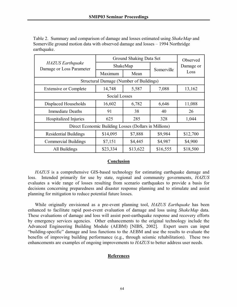
SMIP03 Seminar Proceedings
64
Table 2. Summary and comparison of damage and losses estimated using ShakeMap and Somerville ground motion data with observed damage and losses – 1994 Northridge earthquake.
Conclusion
HAZUS is a comprehensive GIS-based technology for estimating earthquake damage and
loss. Intended primarily for use by state, regional and community governments, HAZUS evaluates a wide range of losses resulting from scenario earthquakes to provide a basis for decisions concerning preparedness and disaster response planning and to stimulate and assist planning for mitigation to reduce potential future losses.
While originally envisioned as a pre-event planning tool, HAZUS Earthquake has been
enhanced to facilitate rapid post-event evaluation of damage and loss using ShakeMap data. These evaluations of damage and loss will assist post-earthquake response and recovery efforts by emergency services agencies. Other enhancements to the original technology include the Advanced Engineering Building Module (AEBM) [NIBS, 2002]. Expert users can input “building-specific” damage and loss functions to the AEBM and use the results to evaluate the benefits of improving building performance (e.g., through seismic rehabilitation). These two enhancements are examples of ongoing improvements to HAZUS to better address user needs.
References
Maximum Mean
Extensive or Complete 14,748 5,587 7,088 13,162
Displaced Households 16,602 6,782 6,646 11,088Immediate Deaths 91 38 40 26
Hospitalized Injuries 625 285 328 1,044
Residential Buildings $14,095 $7,888 $9,984 $12,700Commercial Buildings $7,151 $4,445 $4,987 $4,900
All Buildings $23,334 $13,622 $16,555 $18,500
Direct Economic Building Losses (Dollars in Millions)
HAZUS Earthquake Damage or Loss Parameter
Ground Shaking Data Set
Somerville
Observed Damage or
LossShakeMap
Structural Damage (Number of Buildings)
Social Losses

SMIP03 Seminar Proceedings
65
California Governor’s Office of Emergency Services (OES), 1995. The Northridge Earthquake of January 17, 1994: Report of Data Collection and Analysis, Part A: Damage and Inventory Data. (Sacramento, CA: State of California).
California Governor’s Office of Emergency Services (OES), 1997. The Northridge Earthquake of January 17, 1994: Report of Data Collection and Analysis, Part B: Analysis and Trends. (Sacramento, CA: State of California).
Comerio, Mary C., John D. Landis, Catherine J. Firpo and Juan P. Monzon, 1996. Residential Earthquake Recovery. (Berkeley, CA: California Policy Seminar, University of California).
Earthquake Engineering Research Institute (EERI), 1995. Northridge Earthquake, January 17, 1994, Reconnaissance Report. Supplement C to Vol. 11, April 1995. (Oakland, CA: EERI).
Kircher, Charles A., Aladdin A. Nassar, Onder Kustu and William T. Holmes, 1997a. “Development of Building Damage Functions for Earthquake Loss Estimation,” Earthquake Spectra, Vol. 13, No. 4, (Oakland, California: Earthquake Engineering Research Institute).
Kircher, Charles A., Robert K. Reitherman, Robert V. Whitman and Christopher Arnold, 1997b. “Estimation of Earthquake Losses to Buildings,” Earthquake Spectra, Vol. 13, No. 4, (Oakland, CA: Earthquake Engineering Research Institute).
National Institute of Building Science (NIBS), 1999. HAZUS99 Technical Manual. Developed by the Federal Emergency Management Agency through agreements with the National Institute of Building Sciences (Washington, D.C.: NIBS).
National Institute of Building Science (NIBS), 2002. HAZUS99 Advanced Engineering Building Module Technical and User’s Manual. Developed by the Federal Emergency Management Agency through agreements with the National Institute of Building Sciences (Washington, D.C.: NIBS).
SAC Joint Venture, 1995. Technical report: Characterization of Ground Motions during the Northridge Earthquake of January 17, 1994. SAC 95-03 (Sacramento, CA: SAC Joint Venture).
Wald, David J., Vincent Quitoriano, Tom H. Heaton, Hiroo Kanamori, Craig W. Scrivner, and C. Bruce Worden, 1999. “TriNet ``ShakeMaps'': Rapid Generation of Instrumental Ground Motion and Intensity Maps for Earthquakes in Southern California,” Earthquake Spectra, Vol. 15, No. 3, (Oakland, CA: Earthquake Engineering Research Institute).
Whitman, Robert V., Thalia Anagnos, Charles A. Kircher, Henry J. Lagorio, R. Scoot Lawson and Philip Schneider, 1997. “Development of a National Earthquake Loss Estimation Methodology,” Earthquake Spectra, Vol. 13, No. 4, (Oakland, CA: Earthquake Engineering Research Institute).

SMIP03 Seminar Proceedings
66
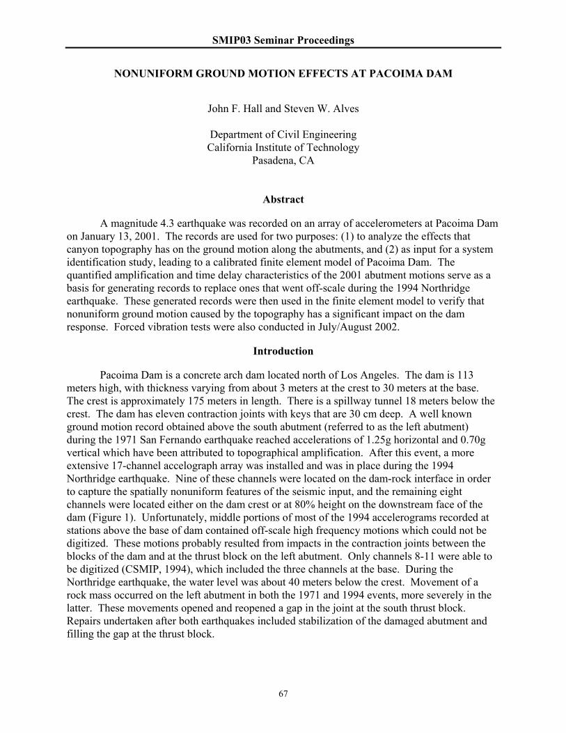
SMIP03 Seminar Proceedings
67
NONUNIFORM GROUND MOTION EFFECTS AT PACOIMA DAM
John F. Hall and Steven W. Alves
Department of Civil Engineering California Institute of Technology
Pasadena, CA
Abstract
A magnitude 4.3 earthquake was recorded on an array of accelerometers at Pacoima Dam on January 13, 2001. The records are used for two purposes: (1) to analyze the effects that canyon topography has on the ground motion along the abutments, and (2) as input for a system identification study, leading to a calibrated finite element model of Pacoima Dam. The quantified amplification and time delay characteristics of the 2001 abutment motions serve as a basis for generating records to replace ones that went off-scale during the 1994 Northridge earthquake. These generated records were then used in the finite element model to verify that nonuniform ground motion caused by the topography has a significant impact on the dam response. Forced vibration tests were also conducted in July/August 2002.
Introduction
Pacoima Dam is a concrete arch dam located north of Los Angeles. The dam is 113 meters high, with thickness varying from about 3 meters at the crest to 30 meters at the base. The crest is approximately 175 meters in length. There is a spillway tunnel 18 meters below the crest. The dam has eleven contraction joints with keys that are 30 cm deep. A well known ground motion record obtained above the south abutment (referred to as the left abutment) during the 1971 San Fernando earthquake reached accelerations of 1.25g horizontal and 0.70g vertical which have been attributed to topographical amplification. After this event, a more extensive 17-channel accelograph array was installed and was in place during the 1994 Northridge earthquake. Nine of these channels were located on the dam-rock interface in order to capture the spatially nonuniform features of the seismic input, and the remaining eight channels were located either on the dam crest or at 80% height on the downstream face of the dam (Figure 1). Unfortunately, middle portions of most of the 1994 accelerograms recorded at stations above the base of dam contained off-scale high frequency motions which could not be digitized. These motions probably resulted from impacts in the contraction joints between the blocks of the dam and at the thrust block on the left abutment. Only channels 8-11 were able to be digitized (CSMIP, 1994), which included the three channels at the base. During the Northridge earthquake, the water level was about 40 meters below the crest. Movement of a rock mass occurred on the left abutment in both the 1971 and 1994 events, more severely in the latter. These movements opened and reopened a gap in the joint at the south thrust block. Repairs undertaken after both earthquakes included stabilization of the damaged abutment and filling the gap at the thrust block.
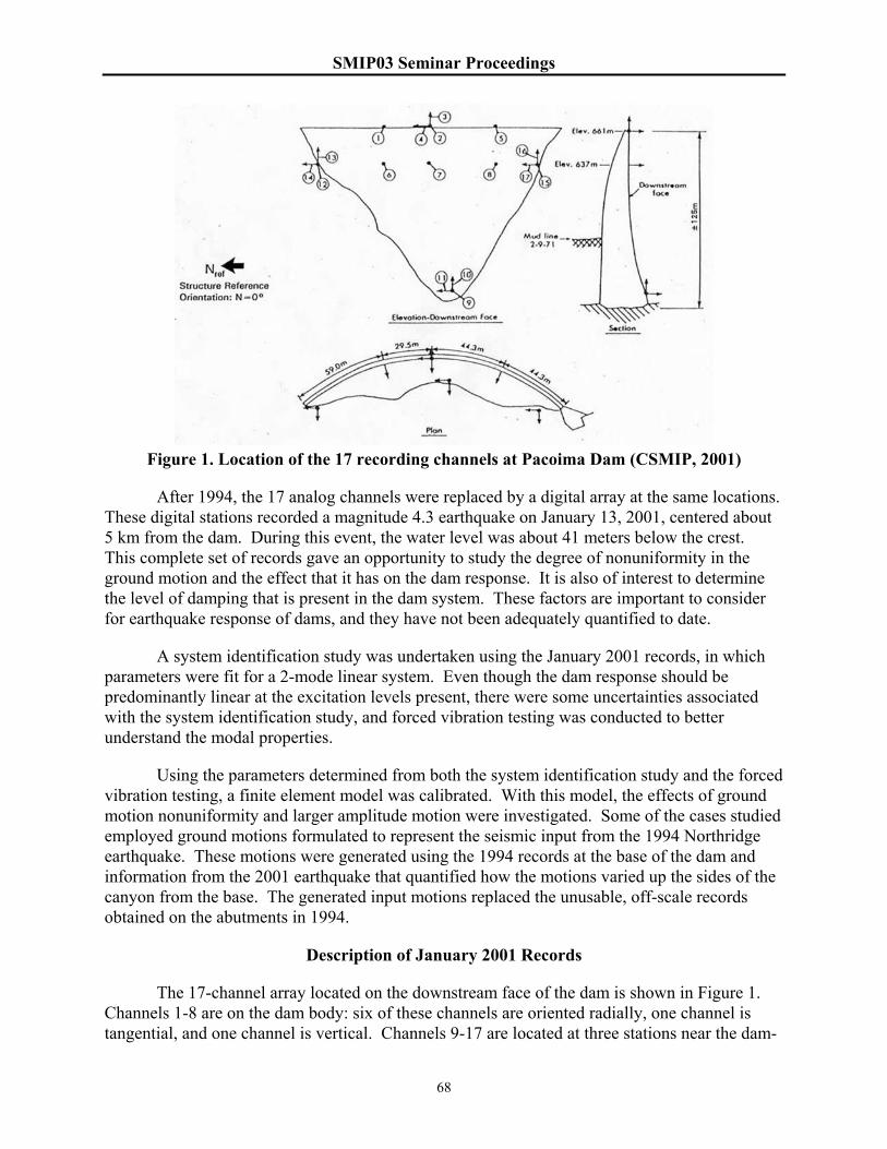
SMIP03 Seminar Proceedings
68
Figure 1. Location of the 17 recording channels at Pacoima Dam (CSMIP, 2001)
After 1994, the 17 analog channels were replaced by a digital array at the same locations. These digital stations recorded a magnitude 4.3 earthquake on January 13, 2001, centered about 5 km from the dam. During this event, the water level was about 41 meters below the crest. This complete set of records gave an opportunity to study the degree of nonuniformity in the ground motion and the effect that it has on the dam response. It is also of interest to determine the level of damping that is present in the dam system. These factors are important to consider for earthquake response of dams, and they have not been adequately quantified to date.
A system identification study was undertaken using the January 2001 records, in which parameters were fit for a 2-mode linear system. Even though the dam response should be predominantly linear at the excitation levels present, there were some uncertainties associated with the system identification study, and forced vibration testing was conducted to better understand the modal properties.
Using the parameters determined from both the system identification study and the forced vibration testing, a finite element model was calibrated. With this model, the effects of ground motion nonuniformity and larger amplitude motion were investigated. Some of the cases studied employed ground motions formulated to represent the seismic input from the 1994 Northridge earthquake. These motions were generated using the 1994 records at the base of the dam and information from the 2001 earthquake that quantified how the motions varied up the sides of the canyon from the base. The generated input motions replaced the unusable, off-scale records obtained on the abutments in 1994.
Description of January 2001 Records
The 17-channel array located on the downstream face of the dam is shown in Figure 1. Channels 1-8 are on the dam body: six of these channels are oriented radially, one channel is tangential, and one channel is vertical. Channels 9-17 are located at three stations near the dam-
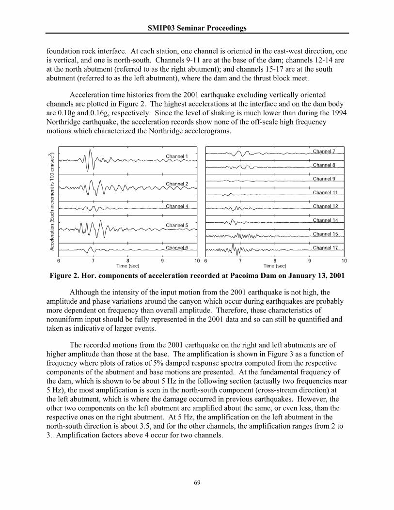
SMIP03 Seminar Proceedings
69
foundation rock interface. At each station, one channel is oriented in the east-west direction, one is vertical, and one is north-south. Channels 9-11 are at the base of the dam; channels 12-14 are at the north abutment (referred to as the right abutment); and channels 15-17 are at the south abutment (referred to as the left abutment), where the dam and the thrust block meet.
Acceleration time histories from the 2001 earthquake excluding vertically oriented channels are plotted in Figure 2. The highest accelerations at the interface and on the dam body are 0.10g and 0.16g, respectively. Since the level of shaking is much lower than during the 1994 Northridge earthquake, the acceleration records show none of the off-scale high frequency motions which characterized the Northridge accelerograms.
Figure 2. Hor. components of acceleration recorded at Pacoima Dam on January 13, 2001
Although the intensity of the input motion from the 2001 earthquake is not high, the amplitude and phase variations around the canyon which occur during earthquakes are probably more dependent on frequency than overall amplitude. Therefore, these characteristics of nonuniform input should be fully represented in the 2001 data and so can still be quantified and taken as indicative of larger events.
The recorded motions from the 2001 earthquake on the right and left abutments are of higher amplitude than those at the base. The amplification is shown in Figure 3 as a function of frequency where plots of ratios of 5% damped response spectra computed from the respective components of the abutment and base motions are presented. At the fundamental frequency of the dam, which is shown to be about 5 Hz in the following section (actually two frequencies near 5 Hz), the most amplification is seen in the north-south component (cross-stream direction) at the left abutment, which is where the damage occurred in previous earthquakes. However, the other two components on the left abutment are amplified about the same, or even less, than the respective ones on the right abutment. At 5 Hz, the amplification on the left abutment in the north-south direction is about 3.5, and for the other channels, the amplification ranges from 2 to 3. Amplification factors above 4 occur for two channels.

SMIP03 Seminar Proceedings
70
Figure 3. Amplification on the abutments of Pacoima Dam referred to motion at the base of
the dam in terms of ratios of response spectra (5% damping)
Another aspect of the nonuniformity in the input is time delay. This quantity can be found between any two motions by integrating their product as a function of time shift between the two. The shift for which this correlation integral is maximized is the time delay, which is listed in Table 1 for respective components of the motions from the base station to the two abutment stations. The delays were computed using the recorded accelerations; the velocities or displacements may also be used and give somewhat shorter delays. As seen, the abutment motions in the horizontal directions lag (positive time delay) the base motions by times ranging from 40 to 66 milliseconds. These delays are a significant fraction of the fundamental period of the dam, which is about 200 milliseconds. Time delays for the vertical component are less, which could be due to the presence of an increased fraction of faster travelling compression waves for the vertical component of ground motion.
E-W Vertical N-S Base to right abutment 0.050 sec 0.024 sec 0.048 sec Base to left abutment 0.040 sec -0.008 sec 0.066 sec
Table 1. Time delays from the base station to the stations on right and left abutments for E-W (stream), vertical and N-S (cross-stream) components of the 2001 earthquake records
A long range goal of collecting ground motion data at the base and sides of canyons, as at Pacoima Dam, is to develop rules for prescribing nonuniform seismic input in safety assessment analyses of dams. Based on the data presented here, one could propose that time delay be a function of elevation and shear wave speed in the rock to account for travel time of seismic waves. For Pacoima Dam, there is about an 84 meter elevation difference between the base and abutment recording stations, and a shear wave velocity for rock of 1200 to 2300 m/sec can be assumed, which is based on a range of previously determined rock properties (Hall, 1988). Using these properties and assuming an upward propagating shear wave result in a time delay of 36 to 70 milliseconds, which includes the range found for the horizontal components of ground motion (Table 1). For the vertical component of ground motion, a time delay in this range could also be appropriate because the shear wave amplitudes are still larger than the compression wave amplitudes (CSMIP, 2001). An additional rule expressing amplification as a function of frequency and elevation could be formulated by averaging the results shown in Figure 3. Such
SMIP03 Seminar Proceedings
71
rules would be applied to components of a reference motion to generate a suite of motions around a canyon. A major difficulty is how to select the reference motion. Should it be considered representative of a bottom site, in which case it would be amplified and time delayed up the canyon sides, or a site near the crest of the dam, in which case it would be attenuated and time forwarded down the canyon sides, or somewhere in between? If the reference motion is to be selected by current standard procedures that are used to produce a uniform motion to be applied to the dam, this becomes an interesting question.
System Identification
System identification was performed using the computer program MODE-ID (Beck and Jennings, 1980; Werner, Beck and Levine, 1987), which models a structure as a linear system with classical normal modes excited by spatially nonuniform ground motion. To run MODE-ID, the user specifies the number of modes to be included and supplies the accelerations recorded on the structure to be used as output response and the accelerations recorded around the structure to be used as input. For Pacoima Dam, channels 1-8 were the output and channels 9-17 were the input. The program uses these time histories to determine the frequencies, damping, shapes, and participation factors for each mode, as well as the pseudo-static response matrix, which produce the best fit to the recorded structural motions. The best fit is determined by minimizing, in the least-squares sense, the mean-square error between the measured and modeled output responses. Theoretically, MODE-ID computes the response of a system which is fixed at the locations of the input, i.e., foundation interaction effects are not included. This is not so clear in the present case of Pacoima Dam where the input is significantly nonuniform and measured at relatively few locations.
MODE-ID allows all parameters, including the pseudo-static matrix, to be adjusted to obtain the best fit, or some parameters can be fixed to predetermined values. Each entry in the pseudo-static matrix corresponds to the response at one of the output channels if one of the input channels is moved a unit amount while the others are held fixed. In the case of Pacoima Dam, allowing the pseudo-static component to be freely adjusted yields results that do not make physical sense. For this reason, the pseudo-static matrix was computed using the finite element model that will be described in a later section. Using this prescribed pseudo-static component, a two-mode model was fit to the 2001 earthquake records. A solution with modal frequencies of 4.74 Hz and 5.05 Hz with damping of 6.2% and 6.6% of critical, respectively, was found. The first mode has a nearly symmetric shape, and the second mode is predominantly antisymmetric. The estimated mode shapes at crest level are shown in Figure 4 with the undeformed crest shown for reference. Shown in Figure 5 are the output accelerations produced by MODE-ID for the horizontal channels at the crest, along with the recorded accelerations. The agreement is good.
Since the first two modal frequencies are closely-spaced, MODE-ID may have difficulty distinguishing some of the modal properties. For example, the mode shapes fit by MODE-ID, as shown in Figure 4, appear to violate orthogonality. The antisymmetric shape may include a component of the symmetric mode. The difficulty could also hold for damping, and, in fact, the measure-of-fit has been shown to be relativley insensitive to the damping ratios, because of a trade-off between participation factors and damping (Beck and Jennings, 1980). However, the modal frequencies are believed to be accurate.

SMIP03 Seminar Proceedings
72
Figure 4. Symmetric and antisymmetric mode shapes computed using MODE-ID, the open
circles are the locations of the crest level stations
Figure 5. Comparison between the recorded accelerations at channels 1, 2, 4 and 5 and the
best-fit accelerations from MODE-ID system identification study
Arch dams typically have two closely-spaced modal frequencies, and these correspond to mode shapes which can be classified as symmetric and antisymmetric. Previous forced vibration tests on Pacoima Dam in April 1980 revealed frequencies of 5.45 Hz and 5.60 Hz for symmetric and antisymmetric modes, respectively (ANCO Engineers, 1982), which are higher than the MODE-ID determined values. The water level during the 1980 tests was about 23 meters below the crest, 18 meters above that during the 2001 earthquake. At these levels, the reservoir should not significantly affect the frequencies, but the 1980 forced vibration determined frequencies would be expected to be even higher if the reservoir was at the 2001 elevation. Damping from the 1980 tests also exceeded that from MODE-ID, but data from those tests were of poor quality and this made it difficult to determine damping accurately. However, even the 6% to 7% damping estimated by MODE-ID seems on the high side compared to forced vibration results from other dams (for example, 1.4% to 4.0% at Morrow Point Dam and 1.8% to 3.1% at

SMIP03 Seminar Proceedings
73
Monticello Dam; see Hall, 1988). In addition, if the MODE-ID methodology is consistent with a rigid foundation, the frequencies with flexible foundation would be even lower than the determined values of 4.74 Hz and 5.05 Hz, increasing the discrepancy with the forced vibration frequencies determined in 1980. To investigate further, additional forced vibration tests were performed on Pacoima Dam.
Forced Vibration Testing
The testing was carried out over one week in July/August 2002. During the testing, the water level was 36 meters below the crest of the dam, 5 meters higher than during the 2001 earthquake. An eccentric mass shaker with force proportional to excitation frequency squared was used to generate the input. Frequency sweeps were conducted from 2.5 Hz to 11.0 Hz for shaking in both the stream and cross-stream directions.
Kinemetrics SS-1 Ranger seismometers were used to measure the motion at 5 locations in two perpendicular, horizontal directions. The Rangers have a response proportional to velocity at frequencies above their natural frequency, which is approximately 1 Hz. The Rangers were placed near the existing accelerometers at the three crest locations on the downstream side, oriented radially and tangentially, (center C, right third R, left quarter L), and at the two locations along the right and left abutments, oriented east-west and north-south, about 24 meters below the crest. The shaker was placed on the upstream side of the dam crest about 3 meters north of Ranger location C. Directions of shaking were radial and tangential at this point; see Figure 6.
Figure 6. Ranger and shaker force locations and directions
For a perfectly symmetric dam with the shaker at the centerline, shaking in the stream direction excites only symmetric modes and shaking cross-stream excites only antisymmetric modes. This is because the motion of the dam centerline is in the stream direction for a symmetric mode and cross-stream for an antisymmetric mode. At Pacoima Dam, due to the lack of sufficient symmetry, the directions of motion at location C for the first symmetric and antisymmetric modes were both primarily in the stream direction with a difference of only 35 degrees between the two directions, compared to a difference of 90 degrees for a perfectly symmetric dam. As a result, there is considerable interference between the two modes for both directions of shaking, and this makes the determination of natural frequencies and damping difficult. Figure 7 shows the interfering resonances of the first symmetric and antisymmetric

SMIP03 Seminar Proceedings
74
modes between 5 Hz and 6 Hz in the response of channel 1 under the stream shake. The amplitude scale in the figure is proportional to the displacement of the dam per unit shaker force.
Figure 7. Frequency response curve for channel 1 at location C for the stream shaking test
One technique to eliminate interference between two modes is to align the direction of shaking perpendicular to the motion of one of the modes, which should eliminate the response of that mode, thus isolating the other one (Duron and Hall, 1986). For the Pacoima Dam data, this was done mathematically by combining the results of the two shaking directions vectorially. As a further enhancement, the pair of Ranger data channels at locations R, C and L were also combined vectorially in order to maximize the peak of the mode being isolated. This method yielded resonant frequency and damping for the antisymmetric mode of 5.70 Hz and 5.0% to 5.5%, respectively, with the damping determined by the half-power method. However, for the symmetric mode the resonant frequency could only be estimated to be between 5.30 Hz to 5.50 Hz with damping of 5.3% estimated only from location L.
A second attempt to isolate the first symmetric and antisymmetric modes was also made, based on the premise that for channels 3 and 5 (radial at locations R and L), the symmetric mode should be in phase and the antisymmetric mode should be out of phase. Using the stream shake, varying amounts of the two radial responses were added until the antisymmetric mode disappeared as much as possible, and varying amounts of the two responses were subtracted until the symmetric mode disappeared as much as possible. Values of natural frequency and damping were determined as 5.45 Hz and 4.0% for the symmetric mode and 5.70 Hz and 4.0% for the antisymmetric mode. A summary of the modal parameters appears in Table 2. The measured mode shapes for the first two modes are plotted in Figure 8.
Mode Natural Frequency Damping Symmetric 5.45 Hz 4.0% < ζ < 5.5%
Antisymmetric 5.70 Hz 4.0% < ζ < 5.5% Table 2. Estimated modal parameters

SMIP03 Seminar Proceedings
75
Figure 8. Symmetric and antisymmetric mode shapes determined from forced vibration
testing, the open circles are the locations of the crest level stations
Comparison of Modal Properties Between Forced Vibration Tests and 2001 Earthquake
A summary of the frequencies and damping values for the first symmetric and antisymmetric modes of Pacoima Dam are presented in Table 3. Included are results from the April 1980 and July/August 2002 forced vibration tests, as well as the MODE-ID determined values from the January 2001 earthquake. In particular, the frequencies of the first symmetric and antisymmetric modes from the July/August 2002 forced vibration tests are 15% and 13% larger, respectively, than those from the earthquake.
Event
Date
Water Level
Freq 1st sym
Damping 1st sym
Freq 1st Anti
Damping 1st Anti
FVT April 1980 -23 m 5.45 Hz ? 7.3% ? 5.60 Hz ? 9.8% ? FVT July/Aug 2002 -36 m 5.45 Hz 4.0%-5.5% 5.70 Hz 4.0%-5.5% EQ Jan 2001 -41 m 4.74 Hz 6.2% 5.05 Hz 6.6%
Table 3. Summary of determined modal frequencies and damping values of Pacoima Dam from two forced vibration tests (FVT) and the January 2001 earthquake (EQ)
The presence of nonlinear effects in structures during earthquakes typically causes resonant frequencies to decrease and effective damping to increase. However, the January 2001 earthquake produced fairly small amplitude motions of Pacoima Dam (peak acceleration and velocity on the crest of 0.16g and 6.2 cm/sec, respectively) which are thought to be still in the linear range. This is confirmed by a finite element simulation reported in the following section for the January 2001 earthquake for which no cracking in the concrete and only a very small amount of joint opening occurs.
Although some of the difference between the forced vibration tests and January 2001 earthquake may be attributed to errors in accurately determining the damping values, as discussed in previous sections, the frequencies are believed to be accurate, and so their differences are harder to explain. A decrease in the frequency of the first symmetric mode from 5.45 Hz during the July/August 2002 forced vibration tests to 4.74 Hz during the January 2001 earthquake requires a reduction in stiffness of the dam system of 32%, and the 5.70 Hz to 5.05 Hz decrease for the antisymmetric mode requires a stiffness reduction of 27%. These changes in stiffness are quite large and would be hard to justify. Nor can the lower frequencies exhibited during the January 2001 earthquake be attributed to difference in water level. First, the levels (Table 3) were all low enough to have only a minor effect on the frequencies. Second, the
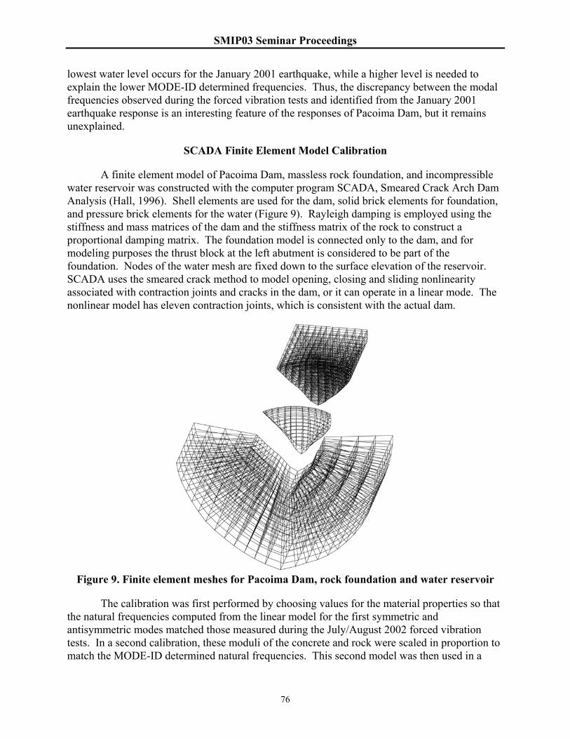
SMIP03 Seminar Proceedings
76
lowest water level occurs for the January 2001 earthquake, while a higher level is needed to explain the lower MODE-ID determined frequencies. Thus, the discrepancy between the modal frequencies observed during the forced vibration tests and identified from the January 2001 earthquake response is an interesting feature of the responses of Pacoima Dam, but it remains unexplained.
SCADA Finite Element Model Calibration
A finite element model of Pacoima Dam, massless rock foundation, and incompressible water reservoir was constructed with the computer program SCADA, Smeared Crack Arch Dam Analysis (Hall, 1996). Shell elements are used for the dam, solid brick elements for foundation, and pressure brick elements for the water (Figure 9). Rayleigh damping is employed using the stiffness and mass matrices of the dam and the stiffness matrix of the rock to construct a proportional damping matrix. The foundation model is connected only to the dam, and for modeling purposes the thrust block at the left abutment is considered to be part of the foundation. Nodes of the water mesh are fixed down to the surface elevation of the reservoir. SCADA uses the smeared crack method to model opening, closing and sliding nonlinearity associated with contraction joints and cracks in the dam, or it can operate in a linear mode. The nonlinear model has eleven contraction joints, which is consistent with the actual dam.
Figure 9. Finite element meshes for Pacoima Dam, rock foundation and water reservoir
The calibration was first performed by choosing values for the material properties so that the natural frequencies computed from the linear model for the first symmetric and antisymmetric modes matched those measured during the July/August 2002 forced vibration tests. In a second calibration, these moduli of the concrete and rock were scaled in proportion to match the MODE-ID determined natural frequencies. This second model was then used in a

SMIP03 Seminar Proceedings
77
SCADA analysis to see if the recorded motions on the dam during the January 2001 earthquake could be reproduced. For this latter exercise, SCADA was modified to accept earthquake ground motion input which was nonuniform along the abutments. All of the calibration studies set the water level to 38 meters below the crest, which was close to the level during both the 2002 forced vibration tests and the 2001 earthquake.
In the first calibration to match the forced vibration determined modal frequencies, the concrete and foundation rock material properties chosen were: Young's moduli of 26,200 MPa (3800 ksi) for concrete and 13,800 MPa (2000 ksi) for rock, Poisson's ratios of 0.20 for concrete and 0.25 for rock, and unit weight of 22.0 kN/m3 (140.0 lb/ft3) for concrete. The computed frequencies for the first symmetric and first antisymmetric modes are 5.45 Hz and 5.69 Hz, respectively, compared to the measured values of 5.45 Hz and 5.70 Hz, respectively. The computed mode shapes at these two frequencies are shown in Figure 10.
Figure 10. Symmetric and antisymmetric mode shapes computed from linear SCADA model calibrated to match forced vibration modal parameters, the open circles are the
locations of the crest level stations
For the calibration to the MODE-ID determined frequencies, a 29% reduction in the Young's moduli to 20,300 MPa (2950 ksi) for the dam concrete and 10,700 MPa (1550 ksi) for the foundation rock reduced the frequencies of the first symmetric and antisymmetric modes computed from the linear model to 4.80 Hz and 5.01 Hz, respectively, close to the MODE-ID frequencies of 4.74 Hz and 5.05 Hz, respectively. The rock modulus is in the range of a rather large variation of field data (Woodward-Lundgren, 1971); it corresponds to a shear wave velocity of about 1300 m/sec. The concrete modulus is in the typical range for dam concrete. The computed mode shapes are similar to those shown in Figure 10.
Another factor to consider for this second calibration is whether the MODE-ID determined frequencies include the effect of foundation flexibility. Since the recorded input motions are on the dam-foundation interface, the theoretical answer is no; however, since the input is only sparsely sampled, this conclusion is questionable. If the finite element model is altered to have a much stiffer foundation, it is found that the symmetric mode is stiffened more than the antisymmetric mode to the point that the antisymmetric mode has the lower frequency. This is not consistent with either the MODE-ID or forced vibration results, and the forced vibration response includes interaction with the foundation. Therefore, it was concluded that the system being modeled by MODE-ID is closer to having a flexible foundation.

SMIP03 Seminar Proceedings
78
As mentioned above, the simulation of the 2001 earthquake response was run with a modified version of SCADA to incorporate nonuniform input. Like the original version of SCADA with uniform ground motion, the nonuniform input is free-field motion, i.e., that which would occur during the earthquake at the dam-foundation interface if the dam were not present. The earthquake is represented by a set of forces which, if applied to the foundation nodes at the interface of the dam with the dam mesh absent, would produce the desired free-field motions. These forces are computed from the nonuniform input displacement and velocity time histories by multiplying them by the foundation stiffness and damping matrices, respectively, and adding. In the analysis, these forces are then applied to the nodes of the interface of the dam and foundation with both meshes present. The water mesh is also included, and the excitation of the water from accelerations of the canyon bottom and sides is performed as in the original version of SCADA except that the distribution of acceleration can be nonuniform.
The records at Pacoima Dam from the base and the two stations on the abutments are not free-field records and so, theoretically, they should be applied with a rigid foundation. However, as mentioned above, the finite element model calibration to the MODE-ID determined frequencies is better with a flexible foundation, and so the simulation of the January 2001 earthquake will use this model with its flexible foundation and apply the recorded motions as if they were free-field motions. This is thought to be a reasonable approximation.
Since the January 2001 accelerograms to be used as input in the simulation were recorded only at the base and the two abutment stations, some interpolation and extrapolation is necessary. Motions at nodes on the north side of the canyon are interpolated from the right abutment and base records, similar for the south side of the canyon using the left abutment and base records. Interpolation is performed channel by channel, and the interpolation at a node is weighted according to the elevation of the node. Before interpolation, any time delay is eliminated by shifting, and then the interpolated record is appropriately re-shifted based on its nodal elevation. For nodes located higher than the abutment stations, larger amplitudes and time delays were extrapolated. Displacement and velocity time histories are integrated from the interpolated/extrapolated acceleration time histories, and used to compute the forces to be applied at the dam-foundation interface. The interpolated/extrapolated accelerations themselves are used for the water excitation.
The simulation of the January 2001 earthquake response used the material properties resulting from the MODE-ID study. With the MODE-ID estimates as a guide, stiffness proportional damping was specified to give modal damping of about 6.7% and 7.0% for the symmetric and antisymmetric modes, respectively. The tensile strength of concrete was set to 3.79 MPa (550 psi).
With nonlinear behavior allowed, the calibrated finite element model subject to the January 2001 earthquake input motions exhibited minimal joint opening, mostly near the crest that was limited to less than 0.03 cm, and there was no cracking. Keys were present to prevent sliding between the joints. The resulting displacement responses at locations corresponding to channels 1, 2, 4 and 5 are compared to the actual recordings in Figure 11. The agreement is good, although the computed response overestimates the displacement during the period of strongest shaking. The agreement between computed and recorded accelerations (not shown) is

SMIP03 Seminar Proceedings
79
not as good. The computed accelerations generally overestimate those of the records, and there are some high frequency spikes that show up in the computed response for channel 4 that are not present in the record. This is due to banging at a joint in the model. However, the agreement is good enough to verify the calibration of the finite element model for use in the earthquake analyses of the next section.
Figure 11. Comparison between the recorded displacements at channels 1, 2, 4 and 5 and
the computed displacements from the SCADA finite element model
Effects of Nonuniform Ground Motion
The finite element model of Pacoima Dam calibrated to the MODE-ID determined properties was used to study the effects of nonuniform ground motion compared to the uniform motion assumption that is commonly used in dam engineering practice. For this purpose, the January 2001 earthquake was considered to be too small to lead to meaningful conclusions. Therefore, it was decided to use the motions from the 1994 Northridge earthquake. However, because of the off-scale problem, only the input records from the base of the dam are available. The motions at the two abutment recording stations had to be generated from these base motions, and this generation was based on the results of the analysis of the January 2001 records.
The amplification factors in Figure 3 were approximated using piecewise linear functions of frequency. These approximate amplification factors are shown in Figure 12. This amplication was applied to the base acceleration histories from the 1994 Northridge earthquake to generate the amplified records at the right and left abutment recording stations. The computation was done by Fourier transforming a record to the frequency domain, scaling it frequency by frequency, and then transforming it back to the time domain. The amplified records were then time shifted to be consistent with the time delays determined from the January 2001 earthquake records (Table 1). As previously argued, the time delay is assumed to be the
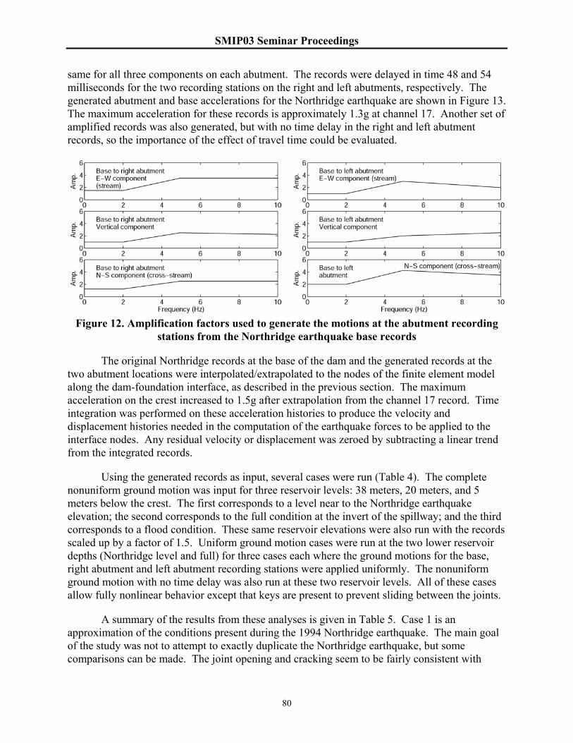
SMIP03 Seminar Proceedings
80
same for all three components on each abutment. The records were delayed in time 48 and 54 milliseconds for the two recording stations on the right and left abutments, respectively. The generated abutment and base accelerations for the Northridge earthquake are shown in Figure 13. The maximum acceleration for these records is approximately 1.3g at channel 17. Another set of amplified records was also generated, but with no time delay in the right and left abutment records, so the importance of the effect of travel time could be evaluated.
Figure 12. Amplification factors used to generate the motions at the abutment recording
stations from the Northridge earthquake base records
The original Northridge records at the base of the dam and the generated records at the two abutment locations were interpolated/extrapolated to the nodes of the finite element model along the dam-foundation interface, as described in the previous section. The maximum acceleration on the crest increased to 1.5g after extrapolation from the channel 17 record. Time integration was performed on these acceleration histories to produce the velocity and displacement histories needed in the computation of the earthquake forces to be applied to the interface nodes. Any residual velocity or displacement was zeroed by subtracting a linear trend from the integrated records.
Using the generated records as input, several cases were run (Table 4). The complete nonuniform ground motion was input for three reservoir levels: 38 meters, 20 meters, and 5 meters below the crest. The first corresponds to a level near to the Northridge earthquake elevation; the second corresponds to the full condition at the invert of the spillway; and the third corresponds to a flood condition. These same reservoir elevations were also run with the records scaled up by a factor of 1.5. Uniform ground motion cases were run at the two lower reservoir depths (Northridge level and full) for three cases each where the ground motions for the base, right abutment and left abutment recording stations were applied uniformly. The nonuniform ground motion with no time delay was also run at these two reservoir levels. All of these cases allow fully nonlinear behavior except that keys are present to prevent sliding between the joints.
A summary of the results from these analyses is given in Table 5. Case 1 is an approximation of the conditions present during the 1994 Northridge earthquake. The main goal of the study was not to attempt to exactly duplicate the Northridge earthquake, but some comparisons can be made. The joint opening and cracking seem to be fairly consistent with

SMIP03 Seminar Proceedings
81
observations. After the earthquake there was a 5 cm opening at the top of the joint between the dam and the thrust block at the left abutment. The opening extended 18 meters down the joint, at which point a large crack extended diagonally into the foundation (Hall, 1995). The residual opening is not present in the model results because the residual input displacement was zero, but the largest computed joint opening does occur at the left abutment and is on the order of the actual observed residual opening. Also, cracking in the model results is limited mostly to elements along the abutments, including elements on the left abutment near the location where the actual crack was observed. Cracking was not reportedly observed in most of the dam body after the Northridge earthquake.
Figure 13. Northridge earthquake accelerations on the abutments (channels 12-17)
generated from the existing base records (channels 9-11)
The maximum arch compressive stresses listed in Table 5 for the cases involving nonuniform input are quite large and exceed somewhat the compressive strength of concrete. For example, the value for Case 1 is 29.66 MPa (4300 psi). Figure 14(a) shows that this large arch compression occurs in a localized region in the corner of the dam at the top of the left abutment. This situation is typical of the other cases. The primary cause of the large arch compressive stresses seems to be the variation of the amplified input displacement along the interface between the dam and foundation. The stresses are fully present in the pseudo-static
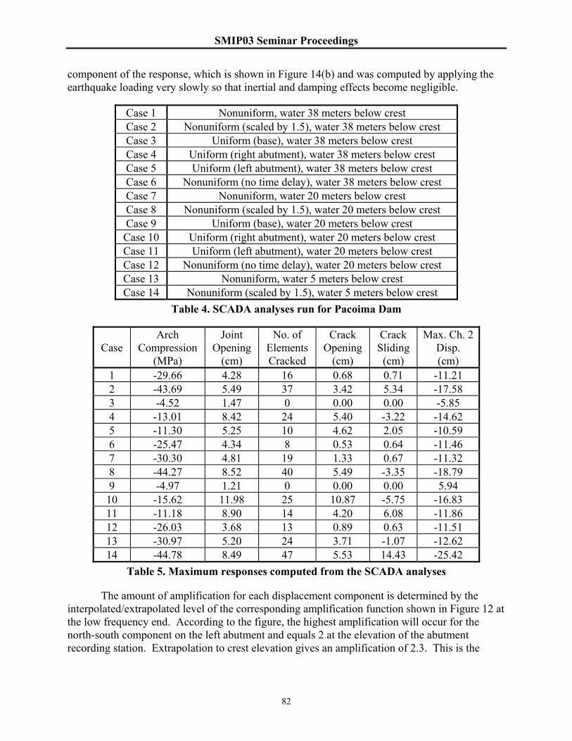
SMIP03 Seminar Proceedings
82
component of the response, which is shown in Figure 14(b) and was computed by applying the earthquake loading very slowly so that inertial and damping effects become negligible.
Case 1 Nonuniform, water 38 meters below crest Case 2 Nonuniform (scaled by 1.5), water 38 meters below crest Case 3 Uniform (base), water 38 meters below crest Case 4 Uniform (right abutment), water 38 meters below crest Case 5 Uniform (left abutment), water 38 meters below crest Case 6 Nonuniform (no time delay), water 38 meters below crest Case 7 Nonuniform, water 20 meters below crest Case 8 Nonuniform (scaled by 1.5), water 20 meters below crest Case 9 Uniform (base), water 20 meters below crest Case 10 Uniform (right abutment), water 20 meters below crest Case 11 Uniform (left abutment), water 20 meters below crest Case 12 Nonuniform (no time delay), water 20 meters below crest Case 13 Nonuniform, water 5 meters below crest Case 14 Nonuniform (scaled by 1.5), water 5 meters below crest
Table 4. SCADA analyses run for Pacoima Dam
Case
Arch Compression
(MPa)
Joint Opening
(cm)
No. of Elements Cracked
Crack Opening
(cm)
Crack Sliding
(cm)
Max. Ch. 2 Disp. (cm)
1 -29.66 4.28 16 0.68 0.71 -11.21 2 -43.69 5.49 37 3.42 5.34 -17.58 3 -4.52 1.47 0 0.00 0.00 -5.85 4 -13.01 8.42 24 5.40 -3.22 -14.62 5 -11.30 5.25 10 4.62 2.05 -10.59 6 -25.47 4.34 8 0.53 0.64 -11.46 7 -30.30 4.81 19 1.33 0.67 -11.32 8 -44.27 8.52 40 5.49 -3.35 -18.79 9 -4.97 1.21 0 0.00 0.00 5.94 10 -15.62 11.98 25 10.87 -5.75 -16.83 11 -11.18 8.90 14 4.20 6.08 -11.86 12 -26.03 3.68 13 0.89 0.63 -11.51 13 -30.97 5.20 24 3.71 -1.07 -12.62 14 -44.78 8.49 47 5.53 14.43 -25.42
Table 5. Maximum responses computed from the SCADA analyses
The amount of amplification for each displacement component is determined by the interpolated/extrapolated level of the corresponding amplification function shown in Figure 12 at the low frequency end. According to the figure, the highest amplification will occur for the north-south component on the left abutment and equals 2 at the elevation of the abutment recording station. Extrapolation to crest elevation gives an amplification of 2.3. This is the

SMIP03 Seminar Proceedings
83
displacement component which is responsible for the large arch compressive stresses in the dam at the top of the left abutment.
Figure 14. Contours of maximum arch compressive stress (MPa) on the upstream face for
(a) Case 1, (b) Case 1 with inertial and damping effects neglected and (c) Case 4
Comparisons of the cases lead to several observations. In general, nonuniform ground motion causes more severe stresses, joint opening and cracking near the abutments (mainly the left one as discussed above) than those computed for the interior of the dam when the water level is 38 meters below the crest. As the water level is raised, the stresses, joint opening and cracking become more severe in the interior of the dam, especially near the upper center. This is due to the higher dynamic response. Of course, when the input motion is scaled up by a factor of 1.5, the response is also more severe. The number of cracked elements approximately doubles for each of the three water levels considered as the input is scaled by 1.5. The cracking is pronounced when the water is 5 meters below the crest and the scale factor is 1.5. For this case, severe cracking and crack sliding are seen in the row of elements approximately 35 meters below the crest. For Pacoima Dam, ground motion this large occurring at the same time as a flood is unlikely. However, if this extreme ground motion and reservoir elevation were the conditions used to assess the safety of a dam, this level of nonlinear behavior might be cause for concern, and more work would be necessary to examine the stability of the dam under these conditions.

SMIP03 Seminar Proceedings
84
The general character of the response under uniform input is quite different from that under nonuniform input. The stresses and levels of cracking and joint opening are relatively low in the region along the abutment, compared to the interior of the dam. When the base records are used as the uniform input, the response is quite mild, with no cracking at all. However, applying the right and left abutment records uniformly generates a more severe response in some ways than the nonuniform input. The joint opening and cracking in the dam interior are more severe than for any region of the dam under nonuniform motion, when corresponding cases are compared. However, the nonlinear behavior along the abutments is generally more severe when nonuniform input is used. The compressive stresses are higher in the upper interior part of the dam for the uniform input, but the left abutment stresses generated by the nonuniform motion are much larger than any stresses generated by the uniform motion (Figure 14(a) and (c)).
When nonuniform motion with no time delay is used, the stresses are generally less severe than when time delay is included. This is most pronounced near the upper part of the abutments. However, some elements near the interior of the dam are slightly more stressed when there is no time delay. The distribution of joint opening is different and the maximum opening is sigificantly larger when delay is included. The extent of cracking is less severe if time delay is omitted. Both the number and the size of cracks are decreased without the delayed input. These results are based on analysis with the water level at the full condition.
Summary and Conclusions
Pacoima Dam has been studied using records obtained from a relatively small magnitude 4.3 earthquake on January 13, 2001. The records from the two abutment stations are amplified and time delayed compared to those from the base of the dam. The complete set of records was used as input (base and abutment stations) and output (dam interior stations) for a system identification study using the computer program MODE-ID. A 2-mode model was used and the fit to the actual records was fairly good. As is often observed with concrete arch dams, the two modes identified have general symmetric and antisymmetric shapes and frequencies which are closely-spaced (4.74 Hz and 5.05 Hz). Damping for both modes was identified between 6% and 7% of critical. While the frequencies are believed to be accurate, the fit is less sensitive to the damping which means the actual range could be noticeably different.
Forced vibration tests were performed in an attempt to more precisely estimate these parameters. However, the two closely-spaced modes had motion in nearly the same direction at the shaker location, which again made it difficult to estimate damping accurately. After a considerable effort to isolate the modes from each other, the damping was determined to lie in a range between 4% and 5.5% for both modes, lower than what was computed by MODE-ID. While the mode shapes were similar to those determined by MODE-ID, the frequencies were significantly higher (5.45 Hz and 5.70 Hz). This discrepancy in the frequencies has not been explained because the dam system should have responded linearly to the small 2001 earthquake. One possibility is some nonlinearity in the slide-prone left abutment, but there is no evidence of such behavior.
The SCADA finite element model was calibrated to match the frequencies and damping determined from MODE-ID, to be consistent with the properties from earthquake excitation. The foundation rock was included in the model even though the input was recorded on the dam-

SMIP03 Seminar Proceedings
85
foundation interface because the best fit to the identified frequencies was obtained with the foundation rock included. Simple interpolation rules were used to generate time histories to be input at each node of the SCADA model. The small January 2001 earthquake response was fairly well replicated in this way, using recorded and computed time histories for comparison, by the SCADA model. This analysis supports the assertion that the dam response was essentially linear.
The 2001 earthquake motion is not large enough to yield results that can be used to study the effects of ground motion nonuniformity on nonlinear aspects of the dam response such as joint opening and concrete cracking. The digitized records measured at the base of the dam during the Northridge earthquake provide much larger excitation, but the input is not complete because the other abutment records were off-scale and could not be processed. So, those other records were generated from the base motion using the frequency-dependent amplification and time delay data determined from the 2001 records. When this motion was input to the SCADA model with the water level the same as that during the Northridge earthquake, the model response was consistent with visual observations that were made after the event.
Several conclusions were drawn from results of the analyses run with the generated Northridge motion. For shaking as experienced during the Northridge earthquake, depending on the water level, joint opening and concrete cracking can be significant contributors to the dam response. As the water level is raised, there is a higher concentration of opening and cracking near the upper center portion of the dam. When the input motion is scaled up by a factor of 1.5, the response is, of course, more severe. With simultaneous earthquake and flood conditions and the Northridge motion magnified by 1.5, cracking is extremely severe with very high compressive stresses at the left abutment. To determine whether the dam would remain stable under these conditions, more work would be required, but these extreme conditions are unlikely for Pacoima Dam.
The SCADA analyses also demonstrated the importance of spatial nonuniformity in the ground motion. Taking the reproduced Northridge motion from a location along the abutment at 80% height of the dam, and applying it uniformly, overestimates the response in the upper part of the dam near the center. However, the response closer to the abutment is underestimated. It was determined that both topographic amplification and seismic wave travel times are important factors in the seismic response of Pacoima Dam, and therefore must be included in any seismic analysis of the dam. The seismic response, particularly near the abutment, receives a significant contribution from the pseudo-static component, which is directly related to the input displacement. This finding (also see Mojtahedi and Fenves, 2000) requires that the nonuniform input displacements be computed with care, for example, without significant integration errors.
In order to further investigate issues relevant to the seismic response of concrete dams, it is recommended that the number of instruments along the abutments at Pacoima Dam be increased. This will allow for the spatial nonuniformity of the motion to be better recorded in subsequent events. These recordings will provide data to support guidelines for generating a set of nonuniform motions from a single characteristic 3-component ground motion determined for a site. Also, if recordings from earthquakes that are even smaller than the 2001 event are obtained and analyzed, more might be learned to clarify the changes in frequencies and damping observed

SMIP03 Seminar Proceedings
86
from forced vibration tests to small seismic events. This will be facilitated with more recording instruments because better characterization of the nonuniform input could lead to more accurate results from system identification studies.
References
ANCO Engineers, 1982. Dynamic Testing of Concrete Dams, report prepared for the National Science Foundation.
Beck, J. L. and P. C. Jennings, 1980. Structural Identification Using Linear Models and Earthquake Records, Earthquake Engineering and Structural Dynamics, Volume 8, Issue No. 2, pp. 145-160.
California Strong Motion Instrumentation Program, 1994. Processed Data for Pacoima Dam - Channels 8 through 11 from the Northridge Earthquake of 17 January 1994, Report OSMS 94-15A.
California Strong Motion Instrumentation Program, 2001. Processed Data for Pacoima Dam - Channels 1 through 17 from the M4.3 Earthquake of 13 January 2001, Report OSMS 01-02.
Duron, Ziyad H. and John F. Hall, 1986. New Techniques in Forced Vibration Testing, Recent Advances in Structural Dynamics: Proceedings of a session sponsored by the Aerospace Division of the American Society of Civil Engineers in conjunction with the ASCE Convention in Seattle, Washington, April 10, 1986, ASCE, pp. 16-33.
Hall, J. F., 1988. The Dynamic and Earthquake Behavior of Concrete Dams: Review of Experimental Behavior and Observational Evidence, Soil Dynamics and Earthquake Engineering, Volume 7, Number 2.
Hall, J. F., 1996. Efficient Nonlinear Seismic Analysis of Arch Dams - User's Manual for SCADA (Smeared Crack Arch Dam Analysis), Report No. EERL 96-01 (modified July 1997), Earthquake Engineering Research Laboratory, Caltech, Pasadena, CA.
Hall, J. F., ed., 1995. Supplement C to Volume 11: Northridge Earthquake of January 17, 1994 Reconnaissance Report, Earthquake Spectra, Volume 1.
Mojtahedi, S. and G. Fenves, 2000. Effect of Contraction Joint Opening on Pacoima Dam in the 1994 Northridge Earthquake, Data Utilization Report CSMIP/00-05 (OSMS 00-07), California Strong Motion Instrumentation Program.
Werner, S. D., J. L. Beck and M. B. Levine, 1987. Seismic Response Evaluation of Meloland Road Overpass Using 1979 Imperial Valley Earthquake Records, Earthquake Engineering and Structural Dynamics, Volume 15, Issue No. 2, pp. 249-274.
Woodward-Lundgren & Associates, 1971. Pacoima Dam - Determination of In Situ Dynamic Elastic Foundation Properties, report prepared for International Engineering Company.
SMIP03 Seminar Proceedings
87
SEISMIC ANALYSIS OF THE INTERSTATE 5 AND HIGHWAY 14 CONNECTOR BRIDGE
Robert K. Dowell
Dowell-Holombo Engineering, Inc. San Diego, California
Abstract
As part of the Strong-Motion Instrumentation Program in California (CSMIP), several bridge structures have been instrumented to record accelerations for the duration of each earthquake event that strikes. The subject of this paper is the investigation of the measured and calculated responses of the heavily instrumented 10-span connector bridge (53-2795F) at the 5/14 Interchange, subjected to a recorded earthquake. A detailed computer model of the bridge structure was developed, allowing comparisons to measured response quantities for many of the 42 sensor locations. In order to compare measured and computed results it was necessary to develop global axes that were common to both the bridge model and structure instrumentation.
Introduction
In order to better understand seismic bridge behavior of a real structure subjected to an actual earthquake, the 10-span connector bridge (53-2795F) at the 5/14 Interchange has been instrumented with 42 channels of data acquisition, measuring accelerations at different locations along the bridge superstructure as well as at the abutments and base of several columns. By integrating recorded accelerations, the velocity and displacement time-history responses are also determined. The recording devices are automatically triggered by small accelerations at the beginning of an earthquake and thus the complete earthquake history is recorded at 0.01 second time intervals at all sensor locations. Of the three earthquakes listed on the CSMIP site for the Sylmar 5/14 Interchange, only the Magnitude 7.1 Hector Mine Earthquake is discussed here, as it produced approximately 50 times more displacement than the other 2 earthquakes. The Hector Mine Earthquake occurred on October 16, 1999 with the epicenter 47 miles ESE of Barstow.
The overall bridge structure and locations of strong-motion instrumentation are shown in
Figure 1. It is a cast-in-place, prestressed, concrete box girder bridge with 10 spans supported by single column bents and pile shafts. There is one expansion joint hinge in the bridge superstructure, placed between Bents 5 and 6. Rather than the hinge being at about the 20% span location, as is typically done in bridge design, the hinge is right in the middle of the span. This is because Span 5 is a very short 26 ft, with 13 ft cantilevers on either side of the hinge. Such a design concept was chosen so that collapse could no occur from unseating of the long span at the hinge, as had occurred to the previous bridge at this site. Thus the connector bridge consists of two separate bridge frames from Abutment 1 to the expansion joint hinge in Span 5 and from this hinge to Abutment 11. The abutments are seat-type, indicating that they are not integral with the bridge superstructure. In order to have similar stiffness’ at all bents, column isolation casings are

SMIP03 Seminar Proceedings
88
provided at some of the bents, which increase the effective length of the columns below the ground line.
Measured results from the Magnitude 7.1 Hector Mine earthquake are provided in this
paper. Also, a discussion of the computer model is given and some comparisons to the measured results are shown. Difficulties in determining the input motions to be used in the model are discussed, as well as how to model the soil at the foundations. Nonlinear and linear time-history analyses as well as modal versus direct time-step integration methods are discussed. It should be noted that development of the detailed structural model is currently underway and that the paper discusses the current state of the modeling as well as modifications that will be made to the model in the near future as part of the ongoing Lifeline Structure Response Project.
Measured Results from Strong-Motion Instrumentation
Loading at the Base of the Structure
This section presents various results that were measured on or near the bridge of interest
from the Hector Mine Earthquake discussed above. In order to compute relative motions between the bridge superstructure and the base input, it is important to understand the overall loading of the bridge and to determine if the abutments and columns were being loaded with different ground motions or essentially the same motion. At first glance, the local longitudinal and transverse displacement time-history responses of Abutments 1 and 11 indicate that they are, indeed, being subjected to different ground motions (Figures 2 and 3), possibly due to the distance between abutments and the variations in soil type and depth. Note that in these figures C2 and C35 are the channel designations for local longitudinal responses at Abutments 1 and 11, respectively. Channels C1 and C33 represent local transverse instrumentation at Abutments 1 and 11, respectively. Throughout the paper the term “local” refers to the instrument direction indicated in Figure 1. Along the bridge superstructure and at the abutments this local direction is tangent to the bridge alignment. At the base of the columns and at the freefield instrumentation, the local alignment of the channels is north, as shown in Figure 1.
Since measured displacement time-history results at the two abutments, presented in
Figures 2 and 3, are given in local coordinates it is not clear if they appear so different from one another due to the varied orientations of the instruments, or if there is a real difference in the ground motions at either end of the bridge. One way to compare the results is to determine the absolute displacement at each point in time for both abutments and plot them on top of each other for the duration of the earthquake. To obtain the absolute displacement requires that the two orthogonal results in plan view be recorded, allowing the square root of the sum of the square of the two orthogonal components to be found for each time interval. The results shown in Figure 4 clearly demonstrate that total displacements at the two abutments and column base of Bent 5 are very similar for the full 80 seconds duration of ground shaking. Note that total displacement is always positive as it represents the distance in plan view from the origin to the displaced location, giving an instantaneous radius. While this result is encouraging, it does not guarantee that the ground motions are the same along the bridge structure, as the angle of the total displacements could be different. For example, at a given point in time the total displacement might be the same at the two abutments but the movement could be in a completely
SMIP03 Seminar Proceedings
89
different direction, resulting in different longitudinal and transverse components. It is, however, very unlikely that the correlation would be as good as shown in Figure 4 for the full 80 seconds of loading unless the angle of displacement also matched closely.
Global responses are compared at the two abutments by converting the displacement
time-history traces of the orthogonal channels into global longitudinal and global transverse directions. In keeping with standard seismic bridge design practice, a line connecting the centerline of the superstructure and the centerline of abutments in plan view is the global longitudinal axis of loading, which is rotated only 1.54 degrees from the north direction indicated in Figure 1, and the global transverse direction of loading is rotated 90 degrees from the global longitudinal axis. These global directions are used to view the measured data and to define the loading directions and input ground motions for the computer model. For each time increment the total displacement is found, as shown in Figure 4, and the angle of rotation is also found in relation to the global axes just defined. When the abutment motions are converted to global axes it is seen that both longitudinal and transverse time-history responses are very similar between the two abutments (Figures 5 and 6). Although not given in these figures, it was determined that the base of Bents 5 and 7 also followed the global abutment displacements very closely. Note that the notation that is now given in the figures shows that global longitudinal and transverse displacements are found from both orthogonal channels at a given location. For example, the legend “Longitudinal C1-2” indicates that local longitudinal and transverse motions from Channels C1 and C2 at Abutment 1 were used to determine the global longitudinal response. The same is required for global transverse displacements.
It is of interest to plot local transverse versus longitudinal displacements, as given in
Figure 7. The distance from the origin to any point on the line represents the total displacement. It can be imagined that this graph is a view of the structure motion from above, in plan view, tracing longitudinal and transverse movements of Abutment 1, and sweeping out the curve given in Figure 7. Of course, in order to compare Abutment 1 and 11 responses on this type of plot the results must be rotated into global coordinates (see Figure 8). This figure shows that the abutment responses are very similar, as indicated previously, and yet they are not exactly the same, with varying amounts of transverse and longitudinal displacements. A line that borders the graph in Figure 8 represents an envelope of maximum displacements.
Joint Openings at Abutments and the Expansion Joint Hinge
Joint motions are given on both sides of each joint in local longitudinal and transverse coordinates at Abutments 1 and 11 and at the expansion joint hinge (Figures 9 through 14). What is clear from these figures is that at both abutments the transverse and longitudinal displacements are very similar on either side of the joint. However, at the expansion joint hinge the two responses on either side of the hinge are vibrating back and forth about each other, indicating relative movement between frames in both longitudinal and transverse directions (Figures 11 and 12). This is somewhat masked because the relative motion between frames is much smaller than the displacement of each frame. Note that the displacement includes the ground motion that the columns and abutments are subjected to.

SMIP03 Seminar Proceedings
90
Relative displacements between frames at the expansion joint hinge were calculated in the longitudinal and transverse directions by taking the difference in the measured displacements on either side of the hinge. The results are presented in Figures 15 and 16, showing a maximum relative transverse displacement of about 0.7 cm and a maximum relative longitudinal displacement of over 1 cm. These figures provide a much clearer picture of the behavior of the two frames at the hinge, showing that they move relatively freely from each other since the expansion joint is at the center of the span and a gap of at least 2 inches is provided between frames to allow for thermal movement. This structure is unusual in that the hinge is at the center of the span and neither span rests on the other, as is typically the case.
Relative Displacements between the Superstructure and Ground Input Motion
Of particular interest is the relative motion between the bridge superstructure and the base input motion or ground motion. This is a little difficult to define because the measured base motion is not identical at all locations along the structure alignment and this information is not available at all of the bents. However, to be consistent throughout the project it is important to clearly define the base motion of the bridge so that it can be subtracted from all other displacements for comparison purposes. This is also important for the structural modeling, as base input accelerations are required to load the model with the measured earthquake. Also, the relative motion from the model between the bridge superstructure and ground will depend on how the base motion is defined, and it must be consistent to have fair comparisons between measured and calculated results. It should be appreciated that to find relative motions requires subtracting large numbers from other large numbers, resulting in increased errors associated with instrument sensitivity and unwanted noise in the data.
As presented earlier, measured global longitudinal and transverse displacement time-
histories at the abutments and at the column bases are very similar to each other and thus it was decided to define Channels C1 and C2 at Abutment 1 as the base motion for all future comparisons and analyses. This completely defines the input motion for the structural model. Note that at this point the vertical motions have not been included in the model. As discussed previously, the model is loaded along global longitudinal and transverse directions with base accelerations determined from Channels C1 and C2 at Abutment 1. Measured relative motions of the bridge superstructure at Bents 5, 6 and 7 are given in Figures 17 through 22 for both transverse and longitudinal directions. Also provided in these figures are results from preliminary time-history analyses of the bridge model. Details of the computer model are discussed in the next section. The analysis results are quite good in the global transverse direction at Bent 5 for the duration of loading, with approximately 1.5 cm of maximum relative displacement between the deck and ground (Figure 18). However, in the global longitudinal direction at Bent 5 the model over-predicts maximum measured displacements by about 50 percent (Figure 17). Maximum calculated relative deck displacements at Bents 6 and 7 are similar to maximum measured response, but the time-history traces do not follow the measured results as closely as in the transverse direction for Bent 5. The maximum measured relative response in the longitudinal direction is about 0.7 cm, while in the transverse direction it is approximately 1.7 cm. Note that measured freefield motion was found to vary significantly from measured abutment and column base motions, and was therefore not used in the present analysis. Clearly this will need to be further investigated.

SMIP03 Seminar Proceedings
91
Computer Model A computer model was developed for the connector structure (Figure 23) using
SAP2000, Version 8 [1]. The bridge superstructure, columns and pile shafts were all modeled with beam elements. Four beam elements were used per span and three beam elements were used per column. Large diameter pile shafts were modeled with nodes spaced at five feet to accommodate longitudinal and transverse soil springs to the model. Initially it was thought that cyclic nonlinear soil springs were needed along the height of the pile shafts. However, measured results from the earthquake have demonstrated that the ground deformations are small enough to assume liner-elastic soil springs. The stiffness’ of the longitudinal and transverse soil springs are based on the initial stiffness given in [2] for the soils listed in the log of test borings. Member geometry follows the centroid of the members in 3-D space. Stiffness values were provided in the local longitudinal and transverse directions at the abutment, based on the size and stress-strain response of expansion joint filler material [3]. With a compressive stress of 0.3625 ksi at 50 percent strain, the modulus of elasticity is 725 ksi.
Results from a modal analysis gave the 1st mode as a transverse response of the 2nd frame
at a natural period of 2.45 seconds (Figure 24). Fourier Amplitude Spectra results show a definite spike at about 2.5 seconds at the same location. This indicates that the overall geometry, mass and stiffness of the model are realistic. Time-history analyses were conducted using modal analyses as well as direct time-stepping procedures and, so long as the damping provided was of the same form and magnitude, the results were virtually identical. Initially, modal time-history analyses were conducted with 2% and then 5% viscous damping. However, all of the analytical deformation results were much larger than measured, and in many cases more than twice the measured displacements. The final analysis results that have been included in this paper have 20 % damping applied to all modes, providing approximately the correct maximum deformations. It is probable that the additional damping is associated with soil response of the large diameter pile shafts and the abutments. Typically, for linear-elastic analysis or RC bridge structures 5% damping is used. For nonlinear analysis a more realistic number is thought to be 2%, with additional damping provided by the hysteretic behavior of the nonlinear elements. It is possible that the additional damping is related to the size of the earthquake motions, which are much smaller than expected from a maximum credible earthquake.
Up to this point in the project the bridge has been modeled with beam elements.
However, the superstructure will be modeled with shell elements. Another possibility is that beam elements will continue to be used to model the superstructure in the global bridge modal and the beam element stiffness properties will be calibrated to results from a breakout shell element model of the superstructure from center-of-span to center-of-span, on either side of a typical bent. All of the behavior is still being modeled as linear-elastic, as the majority of the measured behavior is elastic. However, gapping elements will be provided locally at the interface between the abutment and bridge superstructure, so that no tension can be transferred across this joint. Also, damping elements will be provided to more correctly capture the local increased damping at the soil locations, allowing the damping for the remainder of the structure to be reduced to more realistic values.
SMIP03 Seminar Proceedings
92
The contents of this report were developed under Contract No. 1001-763 from the California Department of Conservation, California Geological Survey, Strong Motion Instrumentation Program. However, these contents do not necessarily represent the policy of that agency nor endorsement by the State Government.
References [1] SAP2000, Version 8, (2002) User’s Manual for computer program. CSI, Inc., Berkeley,
California. [2] Reese, L.C., (2000) User’s Manual for computer program LPILE Plus, Version 4.0,
ENSOFT, Inc., Austin, Texas. [3] Sritharan, S., Preistley, M.J.N., Seible, F., (1997), “Seismic Design and Performance of
Concrete Multi-Column Bents for Bridges”, SSRP-97/03, Division of Structural Engineering, University of California at San Diego.
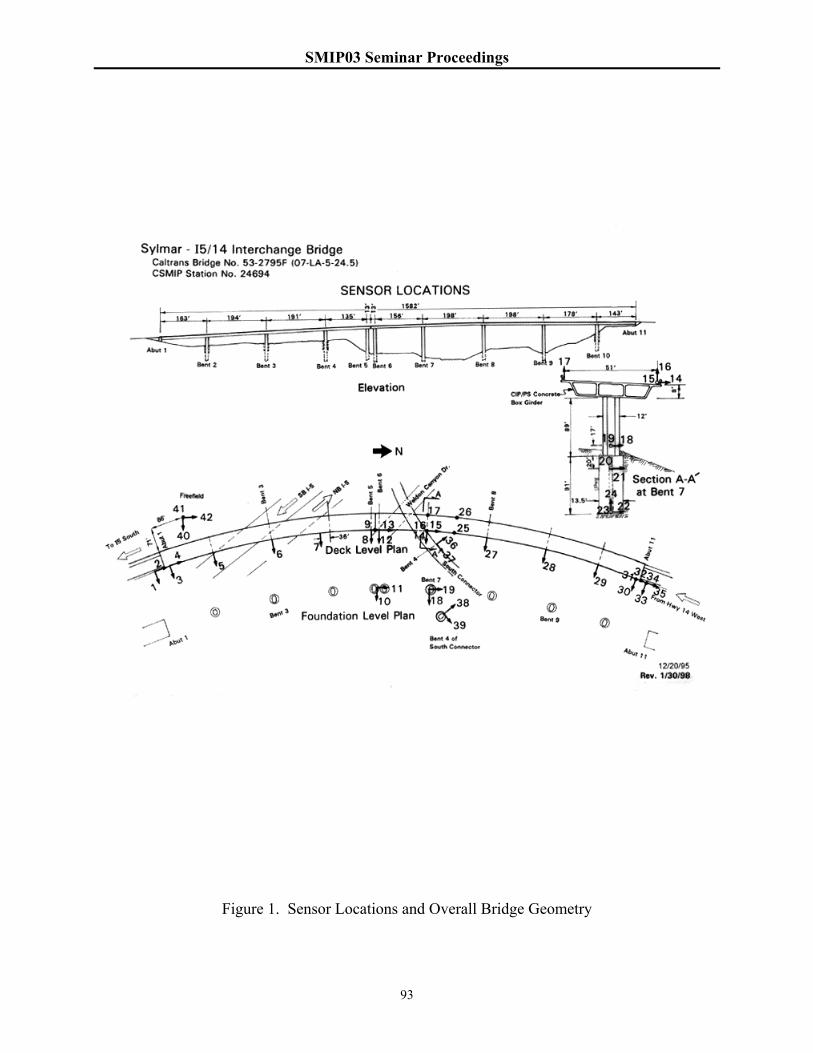
SMIP03 Seminar Proceedings
93
Figure 1. Sensor Locations and Overall Bridge Geometry

SMIP03 Seminar Proceedings
94
Figure 2. Local Longitudinal Response of Abutments 1 and 11
Figure 3. Local Transverse Response of Abutments 1 and 11
-5
-4
-3
-2
-1
0
1
2
3
4
5
0 20 40 60 80
Time (sec.)
Dis
plac
emen
t (cm
)Longitudinal C2
Longitudinal C35
-3
-2
-1
0
1
2
3
0 10 20 30 40 50 60 70 80
Time (sec.)
Dis
plac
emen
t (cm
)
Transverse C1
Transverse C33

SMIP03 Seminar Proceedings
95
Figure 4. Total Response of Abutments 1 and 11 and Base of Bent 5 Column
0
0.5
1
1.5
2
2.5
3
3.5
4
4.5
5
0 20 40 60 80Time (sec.)
Tota
l Dis
plac
emen
t (cm
)
C1-2 (ABUT 1)
C33-35 (ABUT 11)
C10-11 (BENT 5)

SMIP03 Seminar Proceedings
96
Figure 5. Global Longitudinal Response of Abutments 1 and 11
Figure 6. Global Transverse Response of Abutments 1 and 11
-5
-4
-3
-2
-1
0
1
2
3
4
5
0 10 20 30 40 50 60 70 80
Time (sec.)
Dis
plac
emen
t (cm
)Longitudinal C1-2
Longitudinal C33-35
-3
-2
-1
0
1
2
3
0 20 40 60 80
Time (sec.)
Dis
plac
emen
t (cm
)
Transverse C1-2
Transverse C33-35
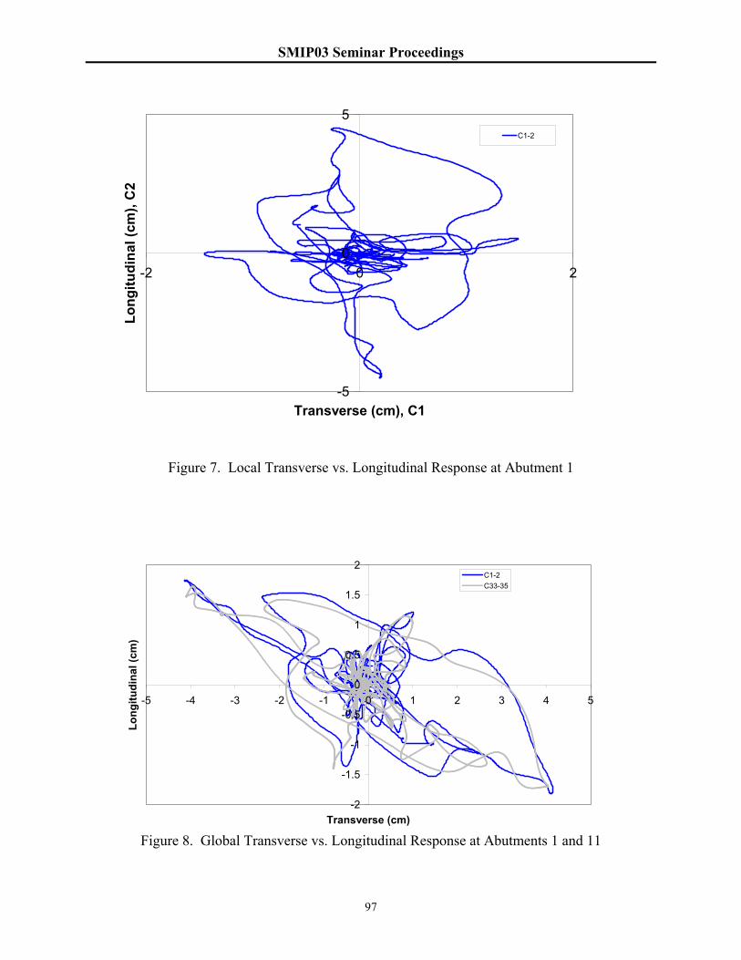
SMIP03 Seminar Proceedings
97
Figure 7. Local Transverse vs. Longitudinal Response at Abutment 1
Figure 8. Global Transverse vs. Longitudinal Response at Abutments 1 and 11
-2
-1.5
-1
-0.5
0
0.5
1
1.5
2
-5 -4 -3 -2 -1 0 1 2 3 4 5
Transverse (cm)
Long
itudi
nal (
cm)
C1-2C33-35
-5
0
5
-2 0 2
Transverse (cm), C1
Long
itudi
nal (
cm),
C2
C1-2

SMIP03 Seminar Proceedings
98
Figure 9. Local Longitudinal Response at Abutment 1
Figure 10. Local Transverse Response at Abutment 1
-2
-1.5
-1
-0.5
0
0.5
1
1.5
2
0 20 40 60 80
Time (sec.)
Dis
plac
emen
t (cm
)
C1C3
-6
-4
-2
0
2
4
6
0 20 40 60 80
Time (sec.)
Dis
plac
emen
t (cm
)
C2C4
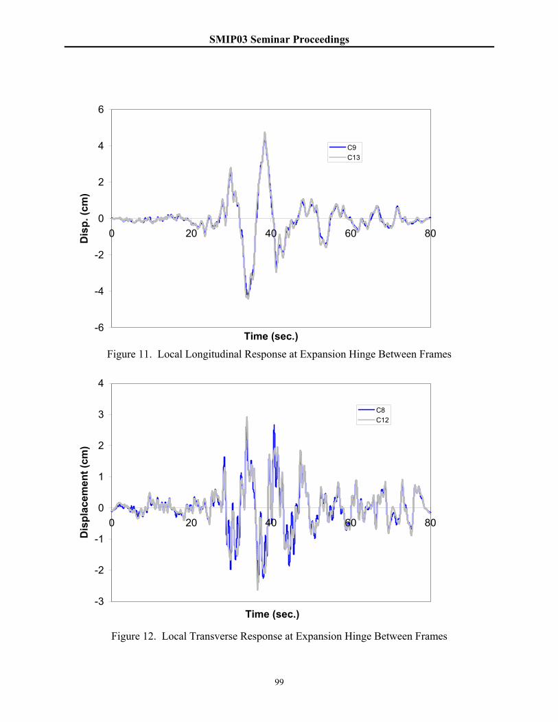
SMIP03 Seminar Proceedings
99
Figure 11. Local Longitudinal Response at Expansion Hinge Between Frames
Figure 12. Local Transverse Response at Expansion Hinge Between Frames
-6
-4
-2
0
2
4
6
0 20 40 60 80
Time (sec.)
Dis
p. (c
m)
C9C13
-3
-2
-1
0
1
2
3
4
0 20 40 60 80
Time (sec.)
Dis
plac
emen
t (cm
)
C8C12
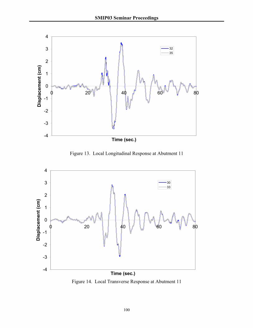
SMIP03 Seminar Proceedings
100
Figure 13. Local Longitudinal Response at Abutment 11
Figure 14. Local Transverse Response at Abutment 11
-4
-3
-2
-1
0
1
2
3
4
0 20 40 60 80
Time (sec.)
Dis
plac
emen
t (cm
)
3235
-4
-3
-2
-1
0
1
2
3
4
0 20 40 60 80
Time (sec.)
Dis
plac
emen
t (cm
)
3033

SMIP03 Seminar Proceedings
101
Figure 15. Relative Longitudinal Response at Expansion Hinge (local)
Figure 16. Relative Transverse Response at Expansion Hinge (local)
-0.8
-0.6
-0.4
-0.2
0
0.2
0.4
0.6
0.8
0 20 40 60 80
Time (sec.)
Rel
ativ
e D
ispl
acem
ent (
cm)
-1.5
-1
-0.5
0
0.5
1
1.5
0 10 20 30 40 50 60 70 80
Time (sec.)
Rel
ativ
e D
ispl
acem
ent (
cm)

SMIP03 Seminar Proceedings
102
Figure 17. Relative Longitudinal Motion Between Deck at Bent 5 and Ground (analysis versus measured)
Figure 18. Relative Transverse Motion Between Deck at Bent 5 and Ground (analysis versus measured)
-0.6
-0.4
-0.2
0
0.2
0.4
0.6
0.8
0 20 40 60 80
Time (sec.)
Rel
ativ
e D
ispl
acem
ent (
cm) Measured
Analysis
Relative Longitudinal Deck MotionBent 5 (C8-9,C1-2)
-1.5
-1
-0.5
0
0.5
1
1.5
2
0 20 40 60 80
Time (sec.)
Rel
ativ
e D
ispl
acem
ent (
cm) Measured
Analysis
Relative Transverse Deck MotionBent 5 (C8-9,C1-2)
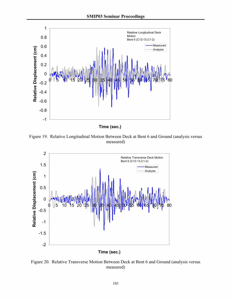
SMIP03 Seminar Proceedings
103
Figure 19. Relative Longitudinal Motion Between Deck at Bent 6 and Ground (analysis versus measured)
Figure 20. Relative Transverse Motion Between Deck at Bent 6 and Ground (analysis versus measured)
-1
-0.8
-0.6
-0.4
-0.2
0
0.2
0.4
0.6
0.8
1
0 5 10 15 20 25 30 35 40 45 50 55 60 65 70 75 80
Time (sec.)
Rel
ativ
e D
ispl
acem
ent (
cm) Measured
Analysis
Relative Longitudinal Deck MotionBent 6 (C12-13,C1-2)
-2
-1.5
-1
-0.5
0
0.5
1
1.5
2
0 5 10 15 20 25 30 35 40 45 50 55 60 65 70 75 80
Time (sec.)
Rel
ativ
e D
ispl
acem
ent (
cm)
MeasuredAnalysis
Relative Transverse Deck MotionBent 6 (C12-13,C1-2)

SMIP03 Seminar Proceedings
104
Figure 21. Relative Longitudinal Motion Between Deck at Bent 7 and Ground (analysis versus measured)
Figure 22. Relative Transverse Motion Between Deck at Bent 7 and Ground (analysis versus measured)
-1
-0.8
-0.6
-0.4
-0.2
0
0.2
0.4
0.6
0.8
1
0 5 10 15 20 25 30 35 40 45 50 55 60 65 70 75 80
Time (sec.)
Rel
ativ
e D
ispl
acem
ent (
cm)
MeasuredAnalysis
Relative Longitudinal Deck MotionBent 7 (C14-15,C1-2)
-2
-1.5
-1
-0.5
0
0.5
1
1.5
2
0 5 10 15 20 25 30 35 40 45 50 55 60 65 70 75 80
Time (sec.)
Rel
ativ
e D
ispl
acem
ent (
cm)
MeasuredAnalysis
Relative Transverse Deck MotionBent 7 (C14-15,C1-2)
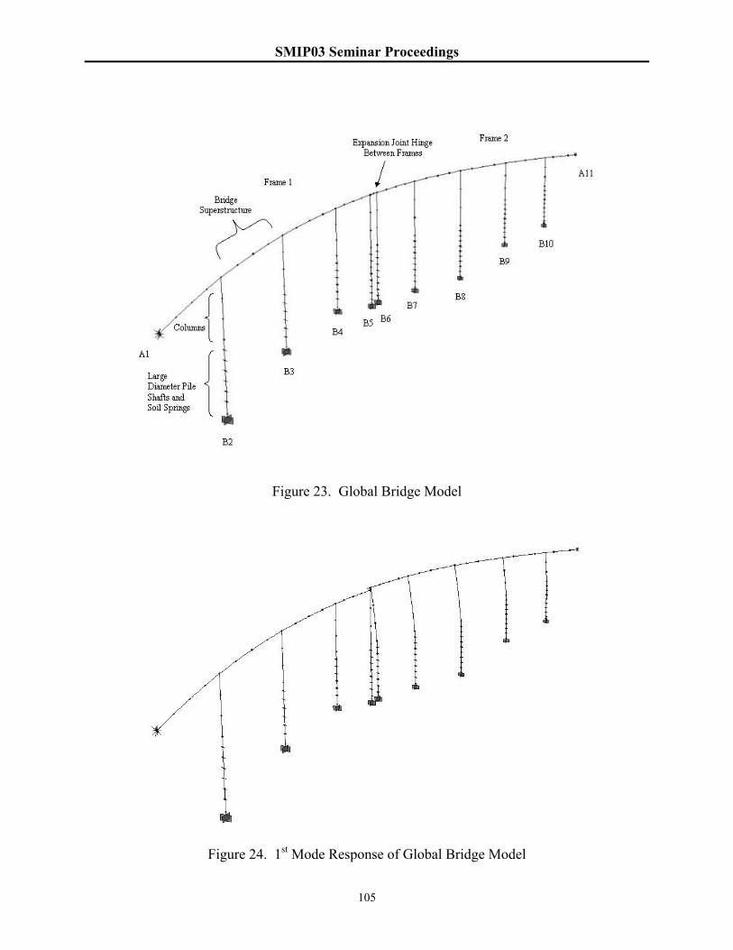
SMIP03 Seminar Proceedings
105
Figure 23. Global Bridge Model
Figure 24. 1st Mode Response of Global Bridge Model

SMIP03 Seminar Proceedings
106

SMIP03 Seminar Proceedings
107
CORRELATION OF OBSERVED BUILDING PERFORMANCE WITH MEASURED GROUND MOTION
Stephanie A. King Hart-Weidlinger, Weidlinger Associates, Inc.
Anne S. Kiremidjian, Pooya Sarabandi, and Dimitris Pachakis
John Blume Earthquake Engineering Center, Stanford University
Abstract
This paper describes results of the CSMIP-funded project to develop correlations of observed building performance with measured ground motion. Much of the information presented in the paper is taken from King et al. (2002), which described the progress of the project to date at last year’s SMIP02 Seminar. Motion-damage relationships in the form of lognormal fragility curves and damage probability matrices have been developed for wood frame, steel moment frame, and concrete frame buildings – building types for which there are enough samples in the database to warrant statistical analysis. The ground motion parameters that were found to exhibit relatively higher correlations with building performance were used in the analysis. Building performance is characterized in terms of damage states and performance levels. The resulting relationships are compared to those published in ATC-13 (ATC, 1985) and HAZUS99 (FEMA, 1999). The comparison shows that the relationships developed in the project are quite different from the published models; however, the loss estimates resulting from the application of the models are similar.
Introduction
Relationships between building performance and ground motion form the core of earthquake loss estimation methodologies, and are also used for structural analysis studies and in the design code formulation process. Currently-used motion-damage relationships are based primarily on models developed from expert opinion, such as ATC-13 (ATC, 1985), or models that combine analytical model results with expert opinion, such as HAZUS99 (FEMA, 1999). Attempts have been made to update the published motion-damage relationships with empirical data collected after damaging earthquakes (see Anagnos et al., 1995). Small improvements have been made to models for specific building types, but typically with the use of proprietary insurance loss data with inferred ground motion information. Following the 1994 Northridge earthquake, an effort was made to systematically document the effects of earthquake shaking on structures adjacent to locations of strong ground motion recordings. The ATC-38 project (ATC, 2000) involved the inspection of more than 500 buildings located near (within 1000 feet of) 30 strong motion recording stations. The resulting database of building characteristic and performance documentation, photos, and strong motion recordings provides a wealth of information for developing new motion-damage relationships

SMIP03 Seminar Proceedings
108
based on non-proprietary empirical data. A similar dataset was also developed following the 1999 Chi-Chi, Taiwan earthquake. The purpose of the CSMIP-funded project discussed in this paper is to develop motion-damage relationships based on the correlation of observed building performance with measured ground motion parameters. The project tasks include: identifying and collecting appropriate datasets; analyzing, interpreting, and archiving data records; developing motion-damage relationships in the form of damage probability matrices and fragility curves; and illustrating the use of the final relationships. The remainder of this paper discusses these tasks in more detail and presents some key results of the project.
Dataset Collection In order to develop meaningful and useful motion-damage relationship that correlate building performance to recorded ground motion data, the datasets have to satisfy certain criteria, including:
• Proximity to free-field ground motion recordings – building should be located close enough to strong motion recordings so that the shaking at the building site can be approximated as the shaking at the instrument site. Also, the building should not have any site-specific geologic conditions that might alter the ground shaking at the site.
• Non-proprietary – the datasets should contain information that is available to the general public so that other researchers may use the raw data, with their own proprietary data or with information collected after future earthquakes.
• Sufficient number of data points –statistical relationships will only be meaningful for those building classes with a large enough sample size.
• Consistent building survey information – building performance data should have been collected in a standard format with consistent inspector interpretation of qualitative and quantitative measures of damage.
• Unbiased with respect to building damage – datasets often include information only for damaged buildings. Statistical relationships will not be meaningful unless the datasets include information for both damaged and undamaged buildings.
The first task of the project was to identify and collect datasets that meet the above criteria, which were found to be very stringent. The following datasets were collected for use in the project:
• ATC-38 – Database on the Performance of Structures Near Strong-Motion Recordings: 1994 Northridge, California Earthquake (ATC, 2000)
• LADiv88 – Rutherford and Chekene Database on the Performance of Rehabilitated Unreinforced Masonry Buildings (Retrofitted According to Los Angeles Division 88 Standards) in the 1994 Northridge, California Earthquake (Lizundia and Holmes, 1997)
• SAC –Database on the Performance of Steel Moment Frame Buildings in the 1994 Northridge, California Earthquake (FEMA, 2000)
SMIP03 Seminar Proceedings
109
• Chi-Chi – Degenkolb Database on the Performance of Buildings Near Strong-Motion Recording Stations (Heintz and Poland, 2001)
Following the collection of the building performance datasets, the accompanying strong ground motion data were identified and collected. For the ATC-38 and Chi-Chi building datasets, the strong ground motion data are included as database tables linked via the attribute containing the building identification number. All buildings in these two datasets could be used in the analysis as they are all located very close (within 1000 feet) of the recording stations. For the SAC and LADiv88 building datasets, only those buildings located near to free-field strong motion recording stations (and on similar site conditions) were extracted from the complete databases. This was done by mapping the building locations in a GIS and overlaying a map of the ground motion recording stations. Two classes of buildings were extracted from their respective datasets – those within 1000 feet of a recording station and those within 1 km of a recording station. The 1000 foot criterion was the approximate distance used in the ATC-38 and Chi-Chi datasets. The 1 km criterion was added so that a sensitivity study of the distance criterion could be done. The strong ground motion data for the stations identified within the vicinity of the SAC and LADiv88 buildings were obtained from several sources including:
• COSMOS – Consortium of Organizations for Strong-Motion Observation Systems Virtual Data Center, which contains links to strong ground motion from the California Division of Mines and Geology, the U.S. Geological Survey, the U.S. Bureau of Reclamation, and the U.S. Army Corps of Engineers (www.cosmos-eq.org)
• PEER – Pacific Earthquake Engineering Research Center Strong Motion Database (peer.berkeley.edu/smcat/)
• NGDC – National Geophysical Data Center Earthquake Strong Motion CD-ROM (www.ngdc.noaa.gov)
Table 1 shows a general distribution of the buildings extracted from the datasets for use in the project.
Ground Motion Analysis Several ground motion parameters were identified as potential candidates for correlation with building performance data. The parameters include those deemed relevant to the intended use of the resulting motion-damage relationships, i.e., they are typically computed in loss estimation and design procedures. The following parameters have been computed and archived for each strong motion data record:
• Time history data parameters (maximum of two horizontal components, average of two horizontal components, and vertical):
• Peak ground acceleration (PGA)
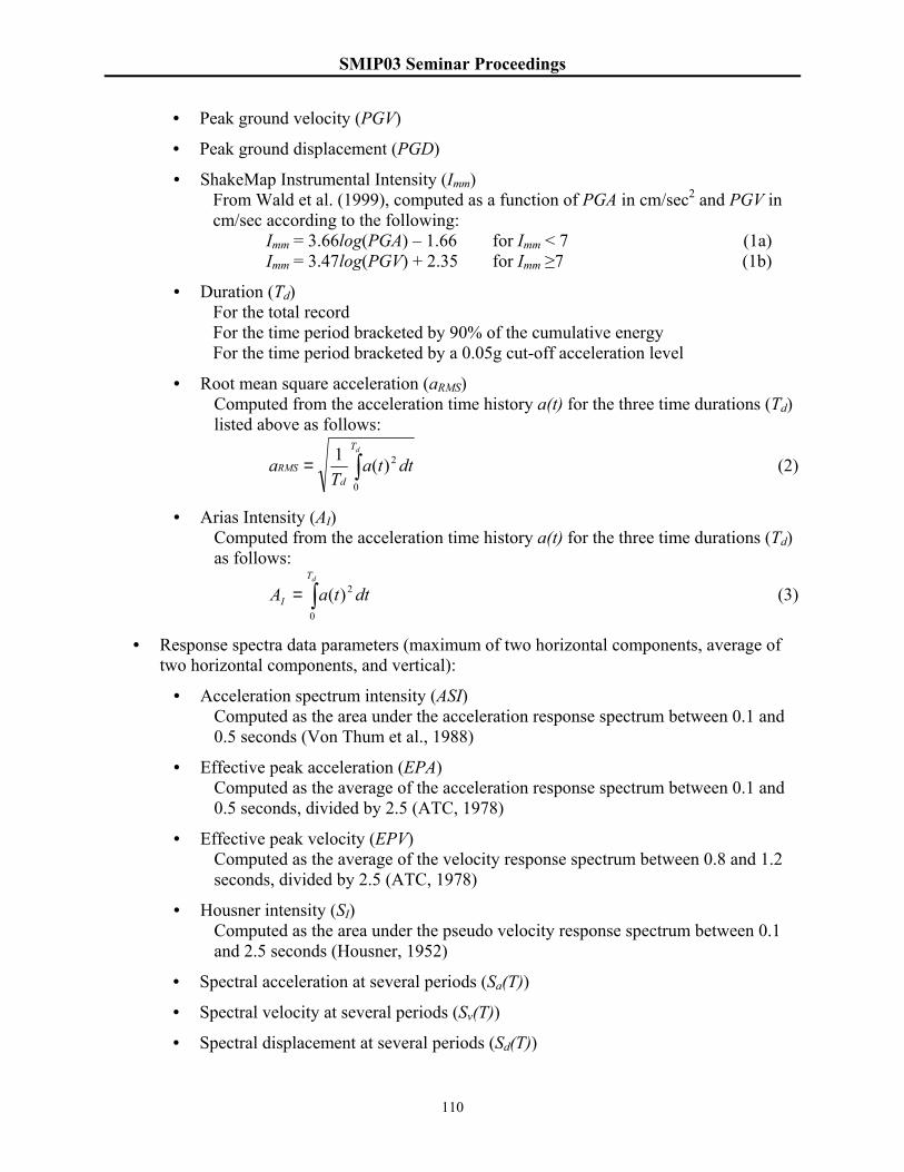
SMIP03 Seminar Proceedings
110
• Peak ground velocity (PGV)
• Peak ground displacement (PGD)
• ShakeMap Instrumental Intensity (Imm) From Wald et al. (1999), computed as a function of PGA in cm/sec2 and PGV in
cm/sec according to the following: Imm = 3.66log(PGA) – 1.66 for Imm < 7 (1a) Imm = 3.47log(PGV) + 2.35 for Imm ≥7 (1b)
• Duration (Td) For the total record For the time period bracketed by 90% of the cumulative energy
For the time period bracketed by a 0.05g cut-off acceleration level
• Root mean square acceleration (aRMS) Computed from the acceleration time history a(t) for the three time durations (Td)
listed above as follows:
∫=dT
dRMS dtta
Ta
0
2)(1 (2)
• Arias Intensity (AI) Computed from the acceleration time history a(t) for the three time durations (Td)
as follows:
∫=dT
I dttaA0
2)( (3)
• Response spectra data parameters (maximum of two horizontal components, average of two horizontal components, and vertical):
• Acceleration spectrum intensity (ASI) Computed as the area under the acceleration response spectrum between 0.1 and
0.5 seconds (Von Thum et al., 1988)
• Effective peak acceleration (EPA) Computed as the average of the acceleration response spectrum between 0.1 and
0.5 seconds, divided by 2.5 (ATC, 1978)
• Effective peak velocity (EPV) Computed as the average of the velocity response spectrum between 0.8 and 1.2
seconds, divided by 2.5 (ATC, 1978)
• Housner intensity (SI) Computed as the area under the pseudo velocity response spectrum between 0.1
and 2.5 seconds (Housner, 1952)
• Spectral acceleration at several periods (Sa(T))
• Spectral velocity at several periods (Sv(T))
• Spectral displacement at several periods (Sd(T))

SMIP03 Seminar Proceedings
111
• Others (not computed, but acquired through map overlays in GIS software):
• Modified Mercalli Intensity (MMI)
• Site class at the recording station site using the 1997 NEHRP Classification (FEMA, 1997)
Table 1 Approximate Distribution of Building Data for Use in Model Development
Building Type Number of Building Records Within 1000 ft of station 1000 ft - 1 km from station Wood Frame 270 Steel Frame 102 57 Concrete Frame 104 Concrete Shear Wall 73 Reinforced Masonry 89 Unreinforced Masonry (URM) 18 Rehabilitated URM 54 116 Precast 10 TOTAL 720 173
Building Response Analysis
The building response datasets were initially analyzed for two purposes – to group the buildings into similar structural classes and to interpret the damage survey information. The grouping of buildings by structural class was done according to the FEMA 310 (FEMA, 1998) model building types shown in Table 2. This classification is similar to that used in the ATC-38 database; however, an important difference is the inclusion of model building type W1A to account for multi-story, multi-unit residences with tuck-under parking. For several of the classes shown in Table 2, the number of data points (see Table 1) was not sufficient to develop motion-damage relationships for those classes. As discussed in the next section, relationships were developed for wood frame, steel moment frame, concrete frame, and concrete shear wall buildings. The building performance information required standardization in terms of damage to structural and nonstructural components. The following classifications are used for structural and nonstructural (if available) damage or performance:
• ATC-13 (ATC, 1985) – Damage states are as follows: • 1 = None = 0% loss • 2 = Slight = 0-1% loss • 3 = Light = 1-10% loss • 4 = Moderate = 10-30% loss • 5 = Heavy = 30-60% loss • 6 = Major = 60-100% loss • 7 = Destroyed = 100% loss
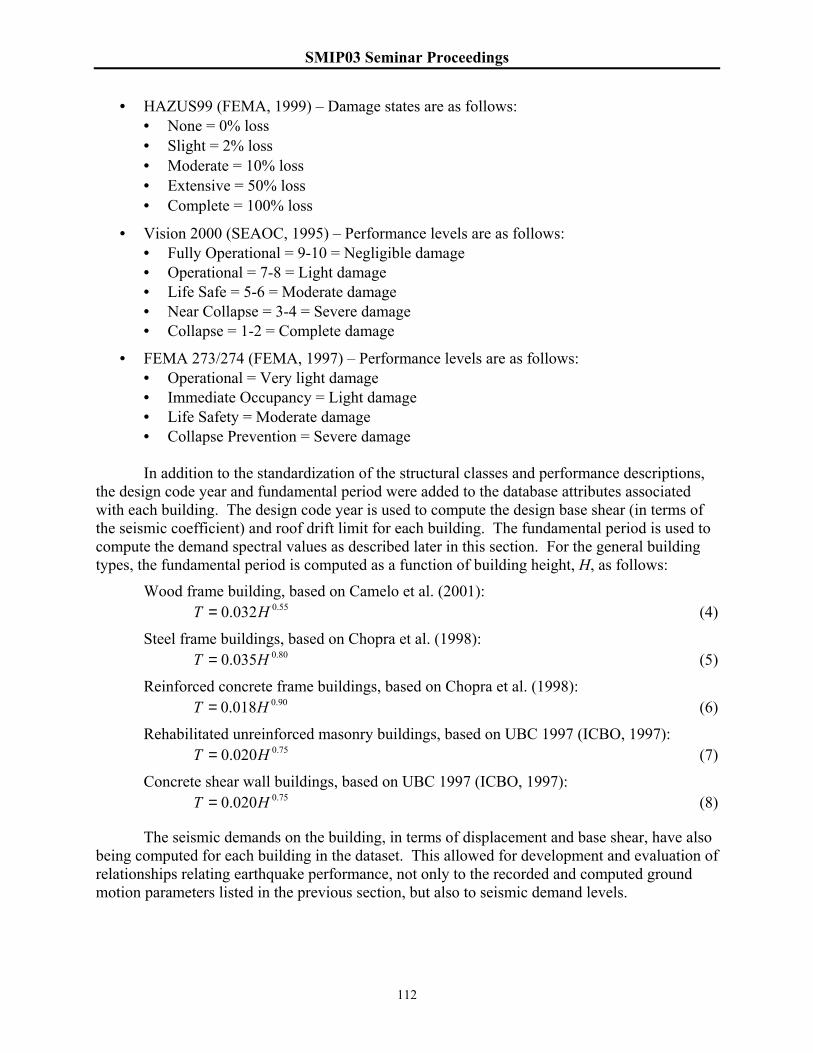
SMIP03 Seminar Proceedings
112
• HAZUS99 (FEMA, 1999) – Damage states are as follows: • None = 0% loss • Slight = 2% loss • Moderate = 10% loss • Extensive = 50% loss • Complete = 100% loss
• Vision 2000 (SEAOC, 1995) – Performance levels are as follows: • Fully Operational = 9-10 = Negligible damage • Operational = 7-8 = Light damage • Life Safe = 5-6 = Moderate damage • Near Collapse = 3-4 = Severe damage • Collapse = 1-2 = Complete damage
• FEMA 273/274 (FEMA, 1997) – Performance levels are as follows: • Operational = Very light damage • Immediate Occupancy = Light damage • Life Safety = Moderate damage • Collapse Prevention = Severe damage
In addition to the standardization of the structural classes and performance descriptions,
the design code year and fundamental period were added to the database attributes associated with each building. The design code year is used to compute the design base shear (in terms of the seismic coefficient) and roof drift limit for each building. The fundamental period is used to compute the demand spectral values as described later in this section. For the general building types, the fundamental period is computed as a function of building height, H, as follows:
Wood frame building, based on Camelo et al. (2001): 55.0032.0 HT = (4)
Steel frame buildings, based on Chopra et al. (1998): 80.0035.0 HT = (5)
Reinforced concrete frame buildings, based on Chopra et al. (1998): 90.0018.0 HT = (6)
Rehabilitated unreinforced masonry buildings, based on UBC 1997 (ICBO, 1997): 75.0020.0 HT = (7)
Concrete shear wall buildings, based on UBC 1997 (ICBO, 1997): 75.0020.0 HT = (8)
The seismic demands on the building, in terms of displacement and base shear, have also being computed for each building in the dataset. This allowed for development and evaluation of relationships relating earthquake performance, not only to the recorded and computed ground motion parameters listed in the previous section, but also to seismic demand levels.

SMIP03 Seminar Proceedings
113
Table 2 Model Building Types (from FEMA, 1998)
W1: Wood Light Frames W1 Single or multiple family dwellings W1A Multi-story, multi-unit residences with open front garages at the first story W2: Wood Frames, Commercial and Industrial S1: Steel Moment Frames S1 Stiff diaphragms S1A Flexible diaphragms S2: Steel Braced Frames S2 Stiff diaphragms S2A Flexible diaphragms S3: Steel Light Frames S4: Steel Frame with Concrete Shear Walls S5: Steel Frame with Infill Masonry Shear Walls S5 Stiff diaphragms S5A Flexible diaphragms C1: Concrete Moment Frames C2: Concrete Shear Wall Buildings C2 Stiff diaphragms C2A Flexible diaphragms C3: Concrete Frame with Infill Masonry Shear Walls C3 Stiff diaphragms C3A Flexible diaphragms PC1: Precast/Tiltup Concrete Shear Walls PC1 Stiff diaphragms PC1A Flexible diaphragms PC2: Precast Concrete Frame PC2 Stiff diaphragms PC2A Flexible diaphragms RM1: Reinforced Masonry Bearing Wall with Flexible Diaphragms RM2: Reinforced Masonry Bearing Wall with Stiff Diaphragms URM: Unreinforced Masonry Bearing Wall URM Stiff diaphragms URMA Flexible diaphragms
The estimate of building displacement demand during the recorded earthquake ground
motion is computed as the spectral displacement demand normalized by the height of the building to obtain a spectral drift ratio. The spectral drift ratio,
dSδ , is calculated by the following:
( ) HTSdSd=δ (9)
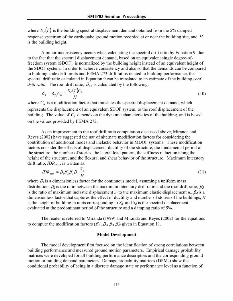
SMIP03 Seminar Proceedings
114
where ( )TSd is the building spectral displacement demand obtained from the 5% damped response spectrum of the earthquake ground motion recorded at or near the building site, and H is the building height.
A minor inconsistency occurs when calculating the spectral drift ratio by Equation 9, due to the fact that the spectral displacement demand, based on an equivalent single degree-of-freedom system (SDOF), is normalized by the building height instead of an equivalent height of the SDOF system. In order to achieve consistency and also so that the demands can be compared to building code drift limits and FEMA 273 drift ratios related to building performance, the spectral drift ratio calculated in Equation 9 can be translated to an estimate of the building roof drift ratio. The roof drift ratio, Rδ , is calculated by the following:
( )H
CTSC dSR d
00 == δδ (10)
where 0C is a modification factor that translates the spectral displacement demand, which represents the displacement of an equivalent SDOF system, to the roof displacement of the building. The value of 0C depends on the dynamic characteristics of the building, and is based on the values provided by FEMA 273.
As an improvement to the roof drift ratio computation discussed above, Miranda and Reyes (2002) have suggested the use of alternate modification factors for considering the contribution of additional modes and inelastic behavior in MDOF systems. These modification factors consider the effects of displacement ductility of the structure, the fundamental period of the structure, the number of stories, the lateral load pattern, the stiffness reduction along the height of the structure, and the flexural and shear behavior of the structure. Maximum interstory drift ratio, IDRmax, is written as:
HS
IDR d4321max ββββ= (11)
where β1 is a dimensionless factor for the continuous model, assuming a uniform mass distribution, β2 is the ratio between the maximum interstory drift ratio and the roof drift ratio, β3 is the ratio of maximum inelastic displacement ui to the maximum elastic displacement ue, β4 is a dimensionless factor that captures the effect of ductility and number of stories of the buildings, H is the height of building in units corresponding to Sd, and Sd is the spectral displacement, evaluated at the predominant period of the structure and a damping ratio of 5%.
The reader is referred to Miranda (1999) and Miranda and Reyes (2002) for the equations to compute the modification factors (β1 , β2, β3, β4) given in Equation 11.
Model Development The model development first focused on the identification of strong correlations between building performance and measured ground motion parameters. Empirical damage probability matrices were developed for all building performance descriptors and the corresponding ground motion or building demand parameters. Damage probability matrices (DPMs) show the conditional probability of being in a discrete damage state or performance level as a function of

SMIP03 Seminar Proceedings
115
the input ground motion or building demand level, which can be a discrete value (e.g., MMI) or a range of values (e.g., PGA). For the areas of strong correlation, fragility curves were developed in the form of lognormal probability distributions following the method outlined in Singhal and Kiremidjian (1996). Fragility curves show the conditional probability of being equal to or exceeding a given damage state or performance level as a function of the ground motion or building demand parameter. Final DPMs were derived from the fragility functions by discretizing the continuous distributions. Figure 1 illustrates the relationship between DPMs, probability distributions, and fragility curves.
DAMAGE PROBABILITY MATRIX Probability (%) of being in a given damage state as a function of PGA for a given building type Damage State PGA 0-0.2g PGA 0.2-0.4g PGA 0.4-0.6g PGA 0.6-0.8g PGA 0.8-1.0g
1, <2% loss 90 80 60 25 20 2, 2-10% loss 10 15 20 40 30 3, 10-30% loss 0 5 15 20 30 4, 30-60% loss 0 0 5 10 15 5, >60% loss 0 0 0 5 5
Figure 1 Illustration of DPM, probability distribution fit, and fragility curve.
Sample Results
Motion-damage relationships were developed for wood frame, steel frame, and concrete frame buildings using data from the 1994 Northridge earthquake and the 1999 Chi-Chi, Taiwan earthquake. Due to space limitations for the paper, only wood frame (class W1) building results will be summarized here. The final project report discusses the results for the other building types and also includes an appendix with a complete set of the motion-damage relationships developed in the project, including lognormal fragility parameters and curves. Fragility functions were developed for the wood frame building class for the following ground motion measures that exhibited relatively higher correlation with building performance: spectral displacement (Sd), Modified Mercalli Intensity (MMI), Instrumental Intensity (IMM),
Cumulative probability distribution based on distributions fit to data
Probability distribution fit to data in DPM for PGA 0.6-0.8g
Damage (% loss) PGA
probability(DS >= 3|PGA) probability

SMIP03 Seminar Proceedings
116
effective peak velocity (EPV), maximum interstory drift ratio (IDRmax), spectral drift ratio (δR), peak ground velocity (PGV), spectral velocity (Sv), root mean square acceleration (RMS), Housner Intensity (HI), peak ground displacement (PGD), spectral acceleration (Sa), peak ground acceleration (PGA), and bracketed duration (Tb). Figures 2 and 3 show sample lognormal fragility curves for wood frame buildings. Figure 2 shows the probability of being in or exceeding the ATC-13 damage states as a function of peak ground acceleration, and Figure 3 shows the probability of being in or exceeding the FEMA 273 performance levels as a function of peak ground displacement.
0
0.2
0.4
0.6
0.8
1
0 0.25 0.5 0.75 1 1.25 1.5
Peak Ground Acceleration (g)
P(D
S>=d
s|Pe
ak G
roun
d A
ccel
erat
ion)
SlightLightModerateHeavyMajorDestroyed
Figure 2 Lognormal fragility curves for W1 buildings and ATC-13 damage states,
conditional on peak ground acceleration. Figure 4 shows a comparison of the lognormal fragility curves conditional on spectral displacement for wood frame buildings published in HAZUS99 (moderate code W1) and as computed in this project. It can be seen in Figure 4 that for the estimated fragility curves, the differences between the various damage states are small, while the HAZUS99 curves for the various damage states are quite distinct. One possible explanation for this observation is that the HAZUS99 fragility curves were estimated based on analysis of one model building of this structural type, while the empirically-derived curves come from many buildings of the same structural type. Hence the performance of the particular building population of the same class is not uniform and for the close values of spectral displacement there are buildings in several damage states. Another source of difference between the HAZUS99 fragility curves and those developed in the project is that the empirical data tend to be concentrated at lower values of spectral displacement and in the lower damage states. For the curves representing higher levels of damage, only a small number of data points were used in the analysis, thus the parameters should be used with caution. Note also that the fragility curves in Figure 4a actually cross at a spectral acceleration value of about 0.9 inches, thus they should not be used beyond this level of displacement.

SMIP03 Seminar Proceedings
117
0
0.2
0.4
0.6
0.8
1
0 10 20 30 40
Peak Ground Displacement (cm)
P(D
S>=d
s|Pe
ak G
roun
d D
ispl
acem
ent)
Immediate OccupancyLife SafetyCollapse Prevention
Figure 3 Lognormal fragility curves for W1 buildings and FEMA 273 performance
levels, conditional on peak ground displacement. Damage probability matrices were developed for the same parameters for which the lognormal fragility curves were. The matrices were developed from the raw empirical data and also derived from the probability distributions defining the fragility curves. Those derived from the fragility curves are discussed here. The damage probability matrix in terms of Modified Mercalli Intensity (MMI) for the W1 building class can be compared to the DPMs published in ATC-13. Figure 5 shows the comparison of the DPM computed in the project for class W1 with the DPM published in ATC-13 for low rise wood frame buildings (class 1). As shown in Figure 5, the two damage probability matrices are quite different. The ATC-13 DPM, developed by fitting beta distributions to expert opinion data, shows a significant increase in probabilities of being in higher damage states for higher levels of MMI. Although, the empirically derived DPM (derived from the lognormal fragility curves) also shows an increase, it is very gradual. Most of the data points are at MMI levels of IX or lower, thus the probabilities associated with MMI X and XI should be used with caution. Note also that the ATC-13 DPM reflects a much narrower probability distribution on damage at each MMI level. Relationships between building performance and strong ground motion are most commonly used for regional and site specific earthquake damage and loss estimation, with the resulting estimates providing information for purposes such as emergency response planning, probabilistic risk assessment, and performance-based design. A few of the relationships developed in this project are discussed above; however, based on this information alone, it is not possible to assess the quality and potential use of the motion-damage relationships. A more meaningful assessment is based on the results of the application of the relationships, i.e., the resulting regional and site-specific damage and loss estimates.
The HAZUS99 (FEMA, 1999) software was used to assess the motion-damage
relationships developed in the project. The study region was Los Angeles County. The software was run using the ShakeMap (USGS, 2003) developed for the M 6.7 1994 Northridge

SMIP03 Seminar Proceedings
118
0
0.25
0.5
0.75
1
0 0.5 1 1.5 2
Spectral Displacement (in)
P[D
S>=d
s|Sp
ectr
al D
ispl
acem
ent]
SlightModerateExtensiveComplete
(a)
0
0.25
0.5
0.75
1
0 2 4 6 8 10
Spectral Displacement (in)
P[D
S>=d
s|Sp
ectr
al D
ispl
acem
ent]
SlightModerateExtensiveComplete
(b)
Figure 4 Fragility curves for W1 buildings, (a) computed in the project and (b) from
HAZUS99. earthquake; first with the default lognormal fragility parameters. Next, the fragility parameters developed in this project for the W1, W2, S1, C1, and C2 building classes were used to replace the default fragility parameters for the corresponding building classes in the HAZUS software. The replacement procedure followed that outlined in Porter et al. (2001). The results of the HAZUS analysis using the default and replaced fragility parameters with the 1994 Northridge earthquake ShakeMap are given in Table 3, which compares the number of buildings in each damage state by general structural class. In general, the number of buildings in the damage states of None and Complete increased significantly, while the number of buildings in the Slight, Moderate, and Extensive damage states decreased. The wood frame buildings show results that are similar to the total building inventory, as would be expected since they make up approximately 92% of the inventory. For concrete frame buildings, the number in the None and
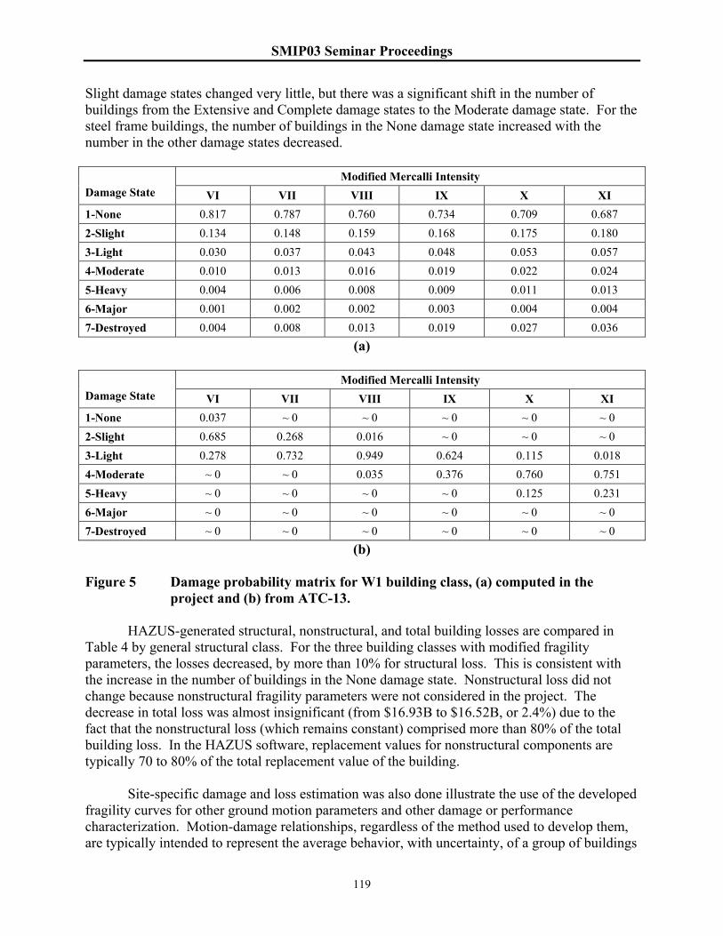
SMIP03 Seminar Proceedings
119
Slight damage states changed very little, but there was a significant shift in the number of buildings from the Extensive and Complete damage states to the Moderate damage state. For the steel frame buildings, the number of buildings in the None damage state increased with the number in the other damage states decreased.
Modified Mercalli Intensity Damage State VI VII VIII IX X XI 1-None 0.817 0.787 0.760 0.734 0.709 0.687 2-Slight 0.134 0.148 0.159 0.168 0.175 0.180 3-Light 0.030 0.037 0.043 0.048 0.053 0.057 4-Moderate 0.010 0.013 0.016 0.019 0.022 0.024 5-Heavy 0.004 0.006 0.008 0.009 0.011 0.013 6-Major 0.001 0.002 0.002 0.003 0.004 0.004 7-Destroyed 0.004 0.008 0.013 0.019 0.027 0.036
(a)
Modified Mercalli Intensity Damage State VI VII VIII IX X XI 1-None 0.037 ~ 0 ~ 0 ~ 0 ~ 0 ~ 0 2-Slight 0.685 0.268 0.016 ~ 0 ~ 0 ~ 0 3-Light 0.278 0.732 0.949 0.624 0.115 0.018 4-Moderate ~ 0 ~ 0 0.035 0.376 0.760 0.751 5-Heavy ~ 0 ~ 0 ~ 0 ~ 0 0.125 0.231 6-Major ~ 0 ~ 0 ~ 0 ~ 0 ~ 0 ~ 0 7-Destroyed ~ 0 ~ 0 ~ 0 ~ 0 ~ 0 ~ 0
(b) Figure 5 Damage probability matrix for W1 building class, (a) computed in the
project and (b) from ATC-13.
HAZUS-generated structural, nonstructural, and total building losses are compared in Table 4 by general structural class. For the three building classes with modified fragility parameters, the losses decreased, by more than 10% for structural loss. This is consistent with the increase in the number of buildings in the None damage state. Nonstructural loss did not change because nonstructural fragility parameters were not considered in the project. The decrease in total loss was almost insignificant (from $16.93B to $16.52B, or 2.4%) due to the fact that the nonstructural loss (which remains constant) comprised more than 80% of the total building loss. In the HAZUS software, replacement values for nonstructural components are typically 70 to 80% of the total replacement value of the building. Site-specific damage and loss estimation was also done illustrate the use of the developed fragility curves for other ground motion parameters and other damage or performance characterization. Motion-damage relationships, regardless of the method used to develop them, are typically intended to represent the average behavior, with uncertainty, of a group of buildings
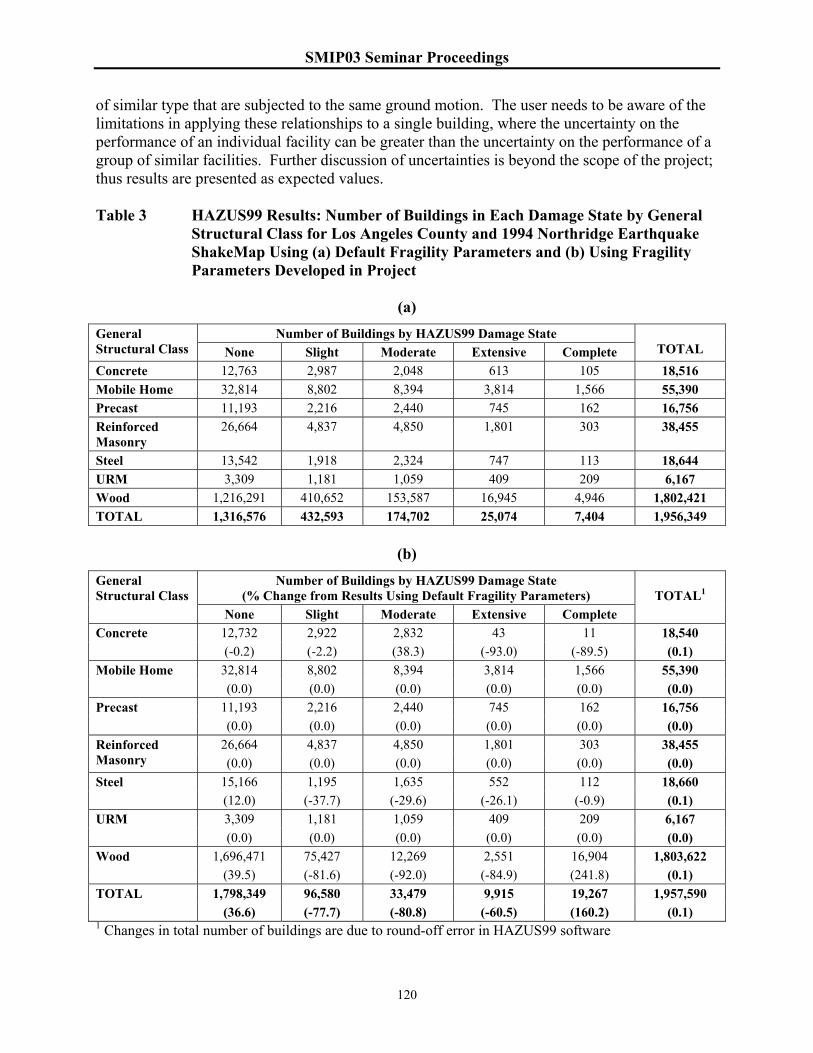
SMIP03 Seminar Proceedings
120
of similar type that are subjected to the same ground motion. The user needs to be aware of the limitations in applying these relationships to a single building, where the uncertainty on the performance of an individual facility can be greater than the uncertainty on the performance of a group of similar facilities. Further discussion of uncertainties is beyond the scope of the project; thus results are presented as expected values. Table 3 HAZUS99 Results: Number of Buildings in Each Damage State by General
Structural Class for Los Angeles County and 1994 Northridge Earthquake ShakeMap Using (a) Default Fragility Parameters and (b) Using Fragility Parameters Developed in Project
(a)
Number of Buildings by HAZUS99 Damage State General Structural Class None Slight Moderate Extensive Complete
TOTAL
Concrete 12,763 2,987 2,048 613 105 18,516 Mobile Home 32,814 8,802 8,394 3,814 1,566 55,390 Precast 11,193 2,216 2,440 745 162 16,756 Reinforced Masonry
26,664 4,837 4,850 1,801 303 38,455
Steel 13,542 1,918 2,324 747 113 18,644 URM 3,309 1,181 1,059 409 209 6,167 Wood 1,216,291 410,652 153,587 16,945 4,946 1,802,421 TOTAL 1,316,576 432,593 174,702 25,074 7,404 1,956,349
(b)
Number of Buildings by HAZUS99 Damage State (% Change from Results Using Default Fragility Parameters)
General Structural Class
None Slight Moderate Extensive Complete
TOTAL1
12,732 2,922 2,832 43 11 18,540 Concrete (-0.2) (-2.2) (38.3) (-93.0) (-89.5) (0.1)
32,814 8,802 8,394 3,814 1,566 55,390 Mobile Home (0.0) (0.0) (0.0) (0.0) (0.0) (0.0)
11,193 2,216 2,440 745 162 16,756 Precast (0.0) (0.0) (0.0) (0.0) (0.0) (0.0)
26,664 4,837 4,850 1,801 303 38,455 Reinforced Masonry (0.0) (0.0) (0.0) (0.0) (0.0) (0.0)
15,166 1,195 1,635 552 112 18,660 Steel (12.0) (-37.7) (-29.6) (-26.1) (-0.9) (0.1) 3,309 1,181 1,059 409 209 6,167 URM (0.0) (0.0) (0.0) (0.0) (0.0) (0.0)
1,696,471 75,427 12,269 2,551 16,904 1,803,622 Wood (39.5) (-81.6) (-92.0) (-84.9) (241.8) (0.1)
1,798,349 96,580 33,479 9,915 19,267 1,957,590 TOTAL (36.6) (-77.7) (-80.8) (-60.5) (160.2) (0.1)
1 Changes in total number of buildings are due to round-off error in HAZUS99 software
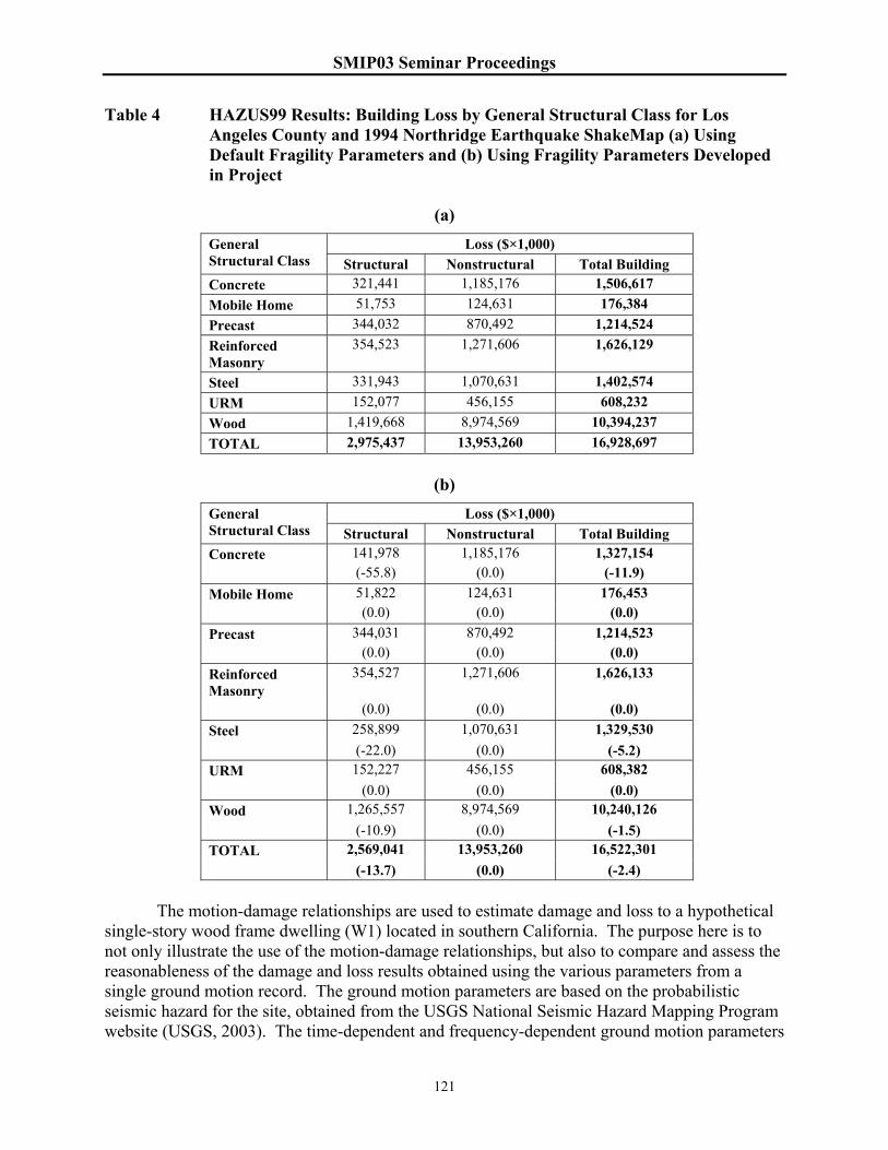
SMIP03 Seminar Proceedings
121
Table 4 HAZUS99 Results: Building Loss by General Structural Class for Los Angeles County and 1994 Northridge Earthquake ShakeMap (a) Using Default Fragility Parameters and (b) Using Fragility Parameters Developed in Project
(a)
Loss ($×1,000) General Structural Class Structural Nonstructural Total Building Concrete 321,441 1,185,176 1,506,617 Mobile Home 51,753 124,631 176,384 Precast 344,032 870,492 1,214,524 Reinforced Masonry
354,523 1,271,606 1,626,129
Steel 331,943 1,070,631 1,402,574 URM 152,077 456,155 608,232 Wood 1,419,668 8,974,569 10,394,237 TOTAL 2,975,437 13,953,260 16,928,697
(b)
Loss ($×1,000) General Structural Class Structural Nonstructural Total Building Concrete 141,978 1,185,176 1,327,154 (-55.8) (0.0) (-11.9) Mobile Home 51,822 124,631 176,453 (0.0) (0.0) (0.0) Precast 344,031 870,492 1,214,523 (0.0) (0.0) (0.0) Reinforced Masonry
354,527 1,271,606 1,626,133
(0.0) (0.0) (0.0) Steel 258,899 1,070,631 1,329,530 (-22.0) (0.0) (-5.2) URM 152,227 456,155 608,382 (0.0) (0.0) (0.0) Wood 1,265,557 8,974,569 10,240,126 (-10.9) (0.0) (-1.5) TOTAL 2,569,041 13,953,260 16,522,301 (-13.7) (0.0) (-2.4)
The motion-damage relationships are used to estimate damage and loss to a hypothetical
single-story wood frame dwelling (W1) located in southern California. The purpose here is to not only illustrate the use of the motion-damage relationships, but also to compare and assess the reasonableness of the damage and loss results obtained using the various parameters from a single ground motion record. The ground motion parameters are based on the probabilistic seismic hazard for the site, obtained from the USGS National Seismic Hazard Mapping Program website (USGS, 2003). The time-dependent and frequency-dependent ground motion parameters
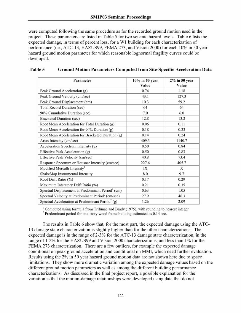
SMIP03 Seminar Proceedings
122
were computed following the same procedure as for the recorded ground motion used in the project. These parameters are listed in Table 5 for two seismic hazard levels. Table 6 lists the expected damage, in terms of percent loss, for a W1 building for each characterization of performance (i.e., ATC-13, HAZUS99, FEMA 273, and Vision 2000) for each 10% in 50 year hazard ground motion parameter for which reasonable lognormal fragility curves could be developed. Table 5 Ground Motion Parameters Computed from Site-Specific Acceleration Data
Parameter 10% in 50 year Value
2% in 50 year Value
Peak Ground Acceleration (g) 0.74 1.18 Peak Ground Velocity (cm/sec) 43.1 127.3 Peak Ground Displacement (cm) 10.3 59.2 Total Record Duration (sec) 64 64 90% Cumulative Duration (sec) 7.0 6.0 Bracketed Duration (sec) 12.8 13.2 Root Mean Acceleration for Total Duration (g) 0.06 0.11 Root Mean Acceleration for 90% Duration (g) 0.18 0.33 Root Mean Acceleration for Bracketed Duration (g) 0.14 0.24 Arias Intensity (cm/sec) 409.3 1140.7 Acceleration Spectrum Intensity (g) 0.50 0.84 Effective Peak Acceleration (g) 0.50 0.83 Effective Peak Velocity (cm/sec) 40.8 73.4 Response Spectrum or Housner Intensity (cm/sec) 227.6 405.7 Modified Mercalli Intensity1 IX X ShakeMap Instrumental Intensity 8.0 9.7 Roof Drift Ratio (%) 0.17 0.29 Maximum Interstory Drift Ratio (%) 0.21 0.35 Spectral Displacement at Predominant Period2 (cm) 0.63 1.05 Spectral Velocity at Predominant Period2 (cm/sec) 27.9 46.3 Spectral Acceleration at Predominant Period2 (g) 1.26 2.09
1 Computed using formula from Trifunac and Brady (1975), with rounding to nearest integer 2 Predominant period for one-story wood frame building estimated as 0.14 sec.
The results in Table 6 show that, for the most part, the expected damage using the ATC-13 damage state characterization is slightly higher than for the other characterizations. The expected damage is in the range of 2-3% for the ATC-13 damage state characterization, in the range of 1-2% for the HAZUS99 and Vision 2000 characterizations, and less than 1% for the FEMA 273 characterization. There are a few outliers, for example the expected damage conditional on peak ground acceleration and conditional on MMI, which need further evaluation. Results using the 2% in 50 year hazard ground motion data are not shown here due to space limitations. They show more dramatic variation among the expected damage values based on the different ground motion parameters as well as among the different building performance characterizations. As discussed in the final project report, a possible explanation for the variation is that the motion-damage relationships were developed using data that do not

SMIP03 Seminar Proceedings
123
adequately represent the high levels of ground motion that correspond to a 2% in 50 year hazard level. Table 6 Expected Damage for Example Site Specific Analysis of Single-Story W1
Building for 10% in 50 Year Hazard Ground Motion
Expected Damage in Percent Loss by Damage or Performance Characterization Type
Parameter
ATC-13 HAZUS99 FEMA 273 Vision 2000 Peak Ground Acceleration (g) 9.5 8.6 0.6 81.4 Peak Ground Velocity (cm/sec) 2.8 1.0 0.5 1.1 Peak Ground Displacement (cm) 5.7 1.0 0.5 1.0 Bracketed Duration (sec) NA 1.3 0.6 1.3 Root Mean Acceleration for Total Duration (g)
3.9 NA 0.8 1.2
Effective Peak Velocity (cm/sec) 2.0 NA NA NA Response Spectrum or Housner Intensity (cm/sec)
NA NA 1.2 1.8
Modified Mercalli Intensity 13.4 NA NA NA ShakeMap Instrumental Intensity 2.4 1.0 0.5 NA Roof Drift Ratio (%) 3.7 2.4 1.7 2.0 Maximum Interstory Drift Ratio (%) 2.4 1.0 0.5 1.0 Spectral Displacement at Predominant Period (cm)
3.2 1.6 0.8 1.6
Spectral Velocity at Predominant Period (cm/sec)
3.0 1.5 0.8 1.5
Spectral Acceleration at Predominant Period (g)
2.5 2.0 1.3 2.0
Note: NA means that probability distribution parameters did not reach convergence.
Conclusions Motion-damage relationships in the form of lognormal fragility curves and corresponding damage probability matrices have been developed from observed building performance data and recorded ground motion within 1000 feet of the buildings. The relationships are for wood frame, steel frame, and concrete frame buildings, for damage characterized by ATC-13 and HAZUS99 damage states and FEMA 273 and Vision 2000 performance levels, and for several ground motion and building demand parameters. A comparison to the ATC-13 and HAZUS99 published damage models shows that the models developed in the project are quite different. The difference is due primarily to the characteristics of the data used in the model development – there is a bias towards lower levels of ground motion and lower levels of damage. Despite the differences in the models themselves, when applied to regional loss estimation via the HAZUS99 software, the total losses for the study region are similar to those computed with the default fragility curve data. For site specific application, the results show that similar losses are produced using different ground motion parameters, and that damage or performance characterization has an influence on the loss values.
SMIP03 Seminar Proceedings
124
The project discussed in this paper utilized a systematic and rigorous method for developing motion-damage relationships from databases of observed building performance and nearby recorded strong ground motion. Although several relationships were developed in the project, the number of building types for which relationships could be developed was limited due to the lack of useful building performance datasets for several types of buildings. In addition, the range of strong ground motion and building demand parameters over which the relationships should be used is limited due to the lack of datasets corresponding to high levels of ground motion. It is hoped that these problems will be remedied by accurate and complete collection of performance data following future seismic events. Utilizing the methods outlined in this project, the developed motion-damage relationships can be updated when new data becomes available, and additional relationships can be developed for other model building types.
Acknowledgements The authors would like to sincerely thank the following individuals who provided valuable data for use in the project: David Bonowitz, Bret Lizundia, and Chris Poland. Ayse Hortacsu provided help with the application of the fragility curves in HAZUS99.
References Anagnos, T., Rojahn, C., and Kiremidjian, A., 1995, NCEER-ATC Joint Study on Fragility of
Buildings, Technical Report NCEER-95-0003, National Center for Earthquake Engineering Research, State University of New York at Buffalo.
ATC, 2000, Database on the Performance of Structures Near Strong-Motion Recordings: 1994 Northridge, California, Earthquake, ATC-38 Report, Applied Technology Council, Redwood City, CA.
ATC, 1985, Earthquake Damage Evaluation Data for California, ATC-13 Report, Applied Technology Council, Redwood City, CA.
ATC, 1978, Tentative Provisions for the Development of Seismic Regulations for Buildings, ATC-3-06 Report, Applied Technology Council, Redwood City, CA.
Camelo, V.S., Beck, J.L., and Hall, J.F., 2001, Dynamic Characteristics of Woodframe Buildings, CUREE-Caltech Woodframe Project Report, Consortium of Universities for Research in Earthquake Engineering, Richmond, CA.
Chopra, A.K., Goel, R.K., and De la Llera, J.C., 1998, “Seismic Code Improvements Based on Recorded Motions of Buildings During Earthquakes,” in Proceedings of SMIP 98 Seminar on Utilization of Strong-Motion Data, California Strong Motion Instrumentation Program, Division of Mines and Geology, Sacramento, CA.
FEMA, 2000, Recommended Seismic Evaluation and Upgrade Criteria for Existing Welded Steel Moment-Frame Buildings, Report FEMA-351, Prepared by the SAC Joint Venture for the Federal Emergency Management Agency, Washington, DC.2000.
FEMA, 1999, HAZUS Earthquake Loss Estimation Methodology, Technical Manual, Prepared by the National Institute of Building Sciences for the Federal Emergency Management Agency, Washington, DC.
SMIP03 Seminar Proceedings
125
FEMA, 1998, Handbook for the Seismic Evaluation of Buildings – A Prestandard, Report FEMA 310, Prepared by the American Society of Civil Engineers for the Federal Emergency Management Agency, Washington, DC.
FEMA, 1997, NEHRP Guidelines for the Seismic Rehabilitation of Buildings, Federal Emergency Management Agency, Report FEMA-273, Washington, DC.
Heintz, J.A. and Poland, C.D., 2001, “Correlating Measured Ground Motion with Observed Damage,” Earthquake Spectra, Supplement A to Volume 17, pp. 110-130.
Housner, G.W., 1959, “Behavior of Structures During Earthquakes,” Journal of the Engineering Mechanics Division, American Society of Civil Engineers, Vol. 85, No. EM14, pp 109-129.
ICBO, 1997, Uniform Building Code, International Conference of Building Officials, Whittier, CA.
King, S.A., Kiremidjian, A.S., Sarabandi, P., and Skokan, M., 2002, “Correlation of Observed Building Performance with Measured Ground Motion,” Proceedings of the SMIP02 Seminar, California Strong Motion Instrumentation Program, California Geological Survey, Sacramento, CA.
Lizundia, B. and Holmes, W.T., 1997, “The performance of rehabilitated URM buildings in the Northridge earthquake,” Proceedings of the NEHRP Conference and Workshop on Research on the Northridge, California Earthquake of January 17, 1994, California Universities for Research in Earthquake Engineering (CUREe), Richmond, California, Vol. III-A, 1998, pages III-116 -- III-123.
Miranda, E. and Reyes, C.J., July 2002, “Approximate Lateral Demands in Multistory Buildings with Nonuniform Stiffness,” Journal of Structural Engineering, Vol. 128, No. 7, pp 840-849.
Miranda, E., April 1999, “Approximate Seismic Lateral Deformation Demands in Multistory Buildings,” Journal of Structural Engineering, Vol. 125, No. 4, pp 417-425.
Porter, K.A., Beck, J.L., Seligson, H.A., Scawthorn, C.R., Tobin, L.T., Young, R., and Boyd, T., 2001, Improving Loss Estimation for Wood Frame Buildings, Final Report on Tasks 4.1 and 4.5 of the CUREE-Caltech Woodframe Project, CUREE, Richmond, CA.
SEAOC, 1995, Performance based seismic engineering of buildings (Vision 2000), Structural Engineers Association of California, Sacramento, CA.
Singhal, A. and Kiremidjian, A.S., 1996, A Method for Earthquake Motion-Damage Relationships with Application to Reinforced Concrete Frames, John A. Blume Earthquake Engineering Center Technical Report No. 119, Stanford University, Stanford, CA.
Trifunac, M.D and Brady, A.G., 1975, “On the correlation of seismic intensity with peaks of recorded strong ground motion,” Bulletin of the Seismological Society of America, Vol. 65, No. 1, pp 139-162.
USGS, 2003, ShakeMap website, www.shakemap.org.
USGS, 2003, National Seismic Hazard Mapping Project website, geohazards.cr.usgs.gov/eq/index.html

SMIP03 Seminar Proceedings
126
Wald, D.J., Quitoriano, V., Heaton, T.H., and Kanamori, H., 1999, “Relationships between Peak Ground Acceleration, Peak Ground Velocity, and Modified Mercalli Intensity in California,” Earthquake Spectra, Vol. 15, No. 3, pp 557-564.

SMIP03 Seminar Proceedings
127
EVALUATION OF NONLINEAR STATIC PROCEDURES USING STRONG-MOTION BUILDING RECORDS
Rakesh K. Goel
Department of Civil & Environmental Engineering California State Polytechnic University, San Luis Obispo, CA
Abstract
The objective of this investigation is to evaluate the FEMA-356 Nonlinear Static Procedure (NSP) and a recently developed Modal Pushover Analysis (MPA) procedure using recorded motions of buildings that were damaged during the 1994 Northridge earthquake. It is found the FEMA-356 NSP typically underestimates the drifts in upper stories and overestimates them in lower stories. The MPA procedure provides much-improved estimates of the response compared to the FEMA-356 NSP. In particular, the MPA procedure, unlike the FEMA-356 NSP, is able to capture the effects of higher modes.
Introduction
Estimating seismic demands at low performance levels, such as life safety and collapse prevention, requires explicit consideration of inelastic behavior of the structure. While nonlinear response history analysis (RHA) is the most rigorous procedure to compute seismic demands, current civil engineering practice prefers to use the nonlinear static procedure (NSP) or pushover analysis specified in the FEMA documents. In early version of FEMA NSP procedure (FEMA, 1997), the seismic demands are computed by nonlinear static analysis of the structure subjected to monotonically increasing lateral forces with an invariant height-wise distribution until a predetermined target displacement is reached. Both the force distribution and target displacement are based on the assumption that the response is controlled by the fundamental mode and that the mode shape remains unchanged after the structure yields.
Obviously, after the structure yields both assumptions are approximate, but investigations (Fajfar and Gaspersic, 1996; Gupta and Krawinkler, 1999; Maison and Bonowitz, 1999; Skokan and Hart, 2000) have led to good estimates of seismic demands. However, such satisfactory predictions of seismic demands are mostly restricted to low- and medium-rise structures for which higher mode effects are likely to be minimal and the inelastic action is distributed throughout the height of the structure (Krawinkler and Seneviratna, 1998).
None of the invariant force distributions can account for a redistribution of inertia forces because of structural yielding and the associated changes in the vibration properties of the structure. To overcome this limitation, several researchers have proposed adaptive force distributions that attempt to follow more closely the time-variant distributions of inertia forces (Bracci et al., 1997; Gupta and Kunnath, 2000). The most recent version of the FEMA NSP (FEMA, 2000), denoted as FEMA-356 NSP, includes one adaptive distribution in the list of lateral load pattern from which two are selected (details are provided latter). While these adaptive force distributions may provide better estimates of seismic demands (Gupta and

SMIP03 Seminar Proceedings
128
Kunnath, 2000), they are conceptually complicated, computationally demanding for routine application in structural engineering practice, and require special purpose computer program to carry out the step-by-step analysis.
Attempts have also been made to consider more than the fundamental vibration mode in pushover analysis. While the Multi-Mode Pushover (MMP) procedure (Paret et al., 1996; Sasaki et al., 1998) provided information on possible failure mechanisms due to higher modes, which may be missed by the standard NSP analyses, other information of interest in the design process, such as story drifts and plastic rotations, could not be computed by this procedure. The “sum-difference” method (Matsumori et al., 1999; Kunnath and Gupta, 2000) provided “useful” information (Kunnath and Gupta, 2000) but lacks theoretical basis.
Recently, a modal pushover analysis (MPA) procedure was developed based on structural dynamics theory that includes the contribution of several modes of vibration (Chopra and Goel, 2001, 2002). This procedure was systematically evaluated (Goel and Chopra, 2002) using six buildings, each analyzed for 20 ground motions. The selected buildings represented two building heights – 9-story and 20-story – and three different seismic regions of the United States – Boston, Seattle, and Los Angeles. The median value of story drifts obtained from the MPA procedure and nonlinear response history analysis (RHA) were compared. It was found that with sufficient number of “modes” included, the height-wise distribution of story drifts estimated by MPA is generally similar to trends noted from nonlinear RHA. Furthermore, the additional error (or bias) in the MPA procedure applied to inelastic structures is small to modest compared to the bias in response spectrum analysis (RSA) applied to elastic structures – the standard analytical tool for the structural engineering profession – unless the building is deformed far into the inelastic region with significant stiffness and strength deterioration.
It is clear from the above review of literature that previous work on development and evaluation of the NSP and improved procedures are based on response of analytical models subjected to recorded and/or simulated earthquake ground motions. Recorded motions of buildings, especially those deformed into the inelastic range, provide a unique opportunity to evaluate such procedures. Therefore, the principal objective of this investigation is to evaluate the FEMA-356 NSP and the MPA procedures using recorded motions of buildings that were deformed beyond the yield limit.
Selected Buildings and Recorded Motions
Recorded motions of buildings that were deformed beyond the yield limit (or damaged) during the earthquake are required for this investigation. For this purpose, four buildings have been identified (Table 1) for which the motions were recorded during the 1994 Northridge earthquake. Of these four buildings, three haven been extensively instrumented by California Strong Motion Instrumentation Program (CSMIP) and one has been nominally instrumented in accordance to the code requirements. The responses of first three of these fours buildings – Van Nuys 7-Story Hotel, Woodland Hills 13-Story, and Sherman Oaks 13-Story – are presented in this paper; the work is in progress on the last building. Following is a brief description of each of these three buildings.
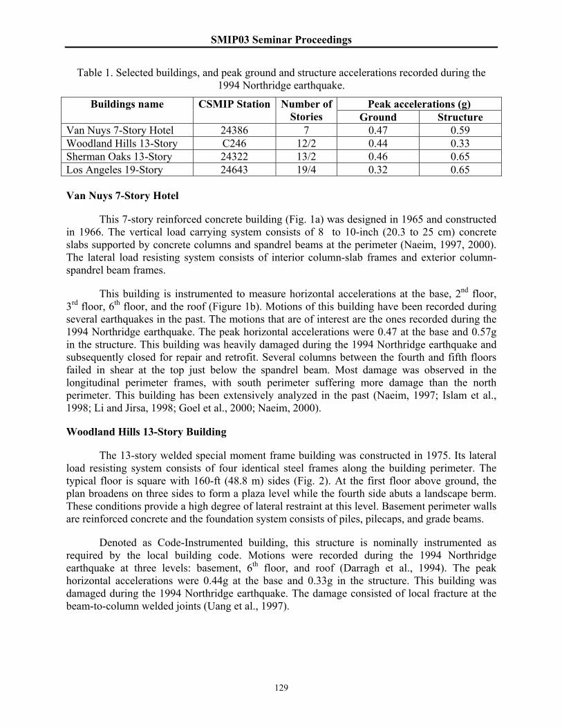
SMIP03 Seminar Proceedings
129
Table 1. Selected buildings, and peak ground and structure accelerations recorded during the 1994 Northridge earthquake.
Peak accelerations (g) Buildings name CSMIP Station Number of Stories Ground Structure
Van Nuys 7-Story Hotel 24386 7 0.47 0.59 Woodland Hills 13-Story C246 12/2 0.44 0.33 Sherman Oaks 13-Story 24322 13/2 0.46 0.65 Los Angeles 19-Story 24643 19/4 0.32 0.65 Van Nuys 7-Story Hotel
This 7-story reinforced concrete building (Fig. 1a) was designed in 1965 and constructed in 1966. The vertical load carrying system consists of 8 to 10-inch (20.3 to 25 cm) concrete slabs supported by concrete columns and spandrel beams at the perimeter (Naeim, 1997, 2000). The lateral load resisting system consists of interior column-slab frames and exterior column-spandrel beam frames.
This building is instrumented to measure horizontal accelerations at the base, 2nd floor, 3rd floor, 6th floor, and the roof (Figure 1b). Motions of this building have been recorded during several earthquakes in the past. The motions that are of interest are the ones recorded during the 1994 Northridge earthquake. The peak horizontal accelerations were 0.47 at the base and 0.57g in the structure. This building was heavily damaged during the 1994 Northridge earthquake and subsequently closed for repair and retrofit. Several columns between the fourth and fifth floors failed in shear at the top just below the spandrel beam. Most damage was observed in the longitudinal perimeter frames, with south perimeter suffering more damage than the north perimeter. This building has been extensively analyzed in the past (Naeim, 1997; Islam et al., 1998; Li and Jirsa, 1998; Goel et al., 2000; Naeim, 2000).
Woodland Hills 13-Story Building
The 13-story welded special moment frame building was constructed in 1975. Its lateral load resisting system consists of four identical steel frames along the building perimeter. The typical floor is square with 160-ft (48.8 m) sides (Fig. 2). At the first floor above ground, the plan broadens on three sides to form a plaza level while the fourth side abuts a landscape berm. These conditions provide a high degree of lateral restraint at this level. Basement perimeter walls are reinforced concrete and the foundation system consists of piles, pilecaps, and grade beams.
Denoted as Code-Instrumented building, this structure is nominally instrumented as required by the local building code. Motions were recorded during the 1994 Northridge earthquake at three levels: basement, 6th floor, and roof (Darragh et al., 1994). The peak horizontal accelerations were 0.44g at the base and 0.33g in the structure. This building was damaged during the 1994 Northridge earthquake. The damage consisted of local fracture at the beam-to-column welded joints (Uang et al., 1997).
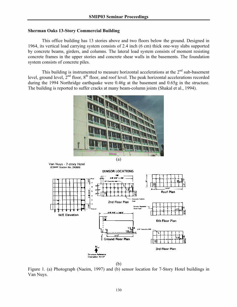
SMIP03 Seminar Proceedings
130
Sherman Oaks 13-Story Commercial Building
This office building has 13 stories above and two floors below the ground. Designed in 1964, its vertical load carrying system consists of 2.4 inch (6 cm) thick one-way slabs supported by concrete beams, girders, and columns. The lateral load system consists of moment resisting concrete frames in the upper stories and concrete shear walls in the basements. The foundation system consists of concrete piles.
This building is instrumented to measure horizontal accelerations at the 2nd sub-basement level, ground level, 2nd floor, 8th floor, and roof level. The peak horizontal accelerations recorded during the 1994 Northridge earthquake were 0.46g at the basement and 0.65g in the structure. The building is reported to suffer cracks at many beam-column joints (Shakal et al., 1994).
(a)
(b)
Figure 1. (a) Photograph (Naeim, 1997) and (b) sensor location for 7-Story Hotel buildings in Van Nuys.

SMIP03 Seminar Proceedings
131
(a)
(b)
Figure 2. (a) Schematic elevation, and (b) plan of the 13-Story building in Woodland Hills (Uang et al., 1997).
(a)
(b) Figure 3. (a) Photograph (Naeim, 1997), and (b) sensor location for 13-story building in Sherman Oaks.

SMIP03 Seminar Proceedings
132
Analysis Methods
Inter-Story Drifts Derived from Recorded Motions
Since buildings are typically instrumented at a limited number of floors, the motions of non-instrumented floors must be inferred from the instrumented floors for calculations of inter-story drifts in all stories. For this purpose, cubic spline interpolation procedure developed earlier by others (Naeim, 1997; De la Llera and Chopra, 1998) is used. The cubic spline interpolation procedure is preferred over the parametric model procedure because it automatically accounts for nonlinearities and time variance of the building parameters. This procedure has been tested (De la Llera and Chopra, 1998) and found to he highly accurate in estimating the motions of non-instrumented floors.
The cubic spline interpolation is performed on the building deformation (relative to the base) instead of the floor accelerations as traditionally done. This is because splines satisfy conditions of continuity and differentiability of second order at the interpolation points (i.e., instrumented floors in this case) and hence provide smooth shapes, as it should be, for the displacement field of the building.
Once the time variation of deformations of all floors have been developed using the cubic spline interpolation procedure, inter-story drifts at each time instant is computed from
1( ) ( ) ( )j j jt u t u tδ −= − (1)
in which ( )j tδ is the inter-story drift in the jth story, and ( )ju t and 1( )ju t− are the deformations at the jth and j-1th floor levels at time t. Once the time histories of the inter-story drifts have been developed, peak values in the jth story, joδ , is be computed as the absolute maximum value over time. These values, denoted as “derived” inter-story drifts, would be used to evaluate the FEMA-356 NSP and MPA procedures.
Modal Decomposition of Recorded Motions
The contributions of various natural modes of vibration of the building to the total displacement can be extracted from the recorded (or interpolated) motions by using the standard modal analysis method (Chopra, 2001); the procedure would lead to exact modal contributions for buildings that remain elastic but approximate for inelastic buildings. This procedure has been used in our previous research (Chopra and Goel, 2001, 2002) to investigate the contributions of higher modes in inelastic buildings.
The contribution of the nth mode to total deformation at floor level j and time instant t is given by:
( )( )T
njn jnT
n n
tu t φ=
mum
φφ φ
(2)
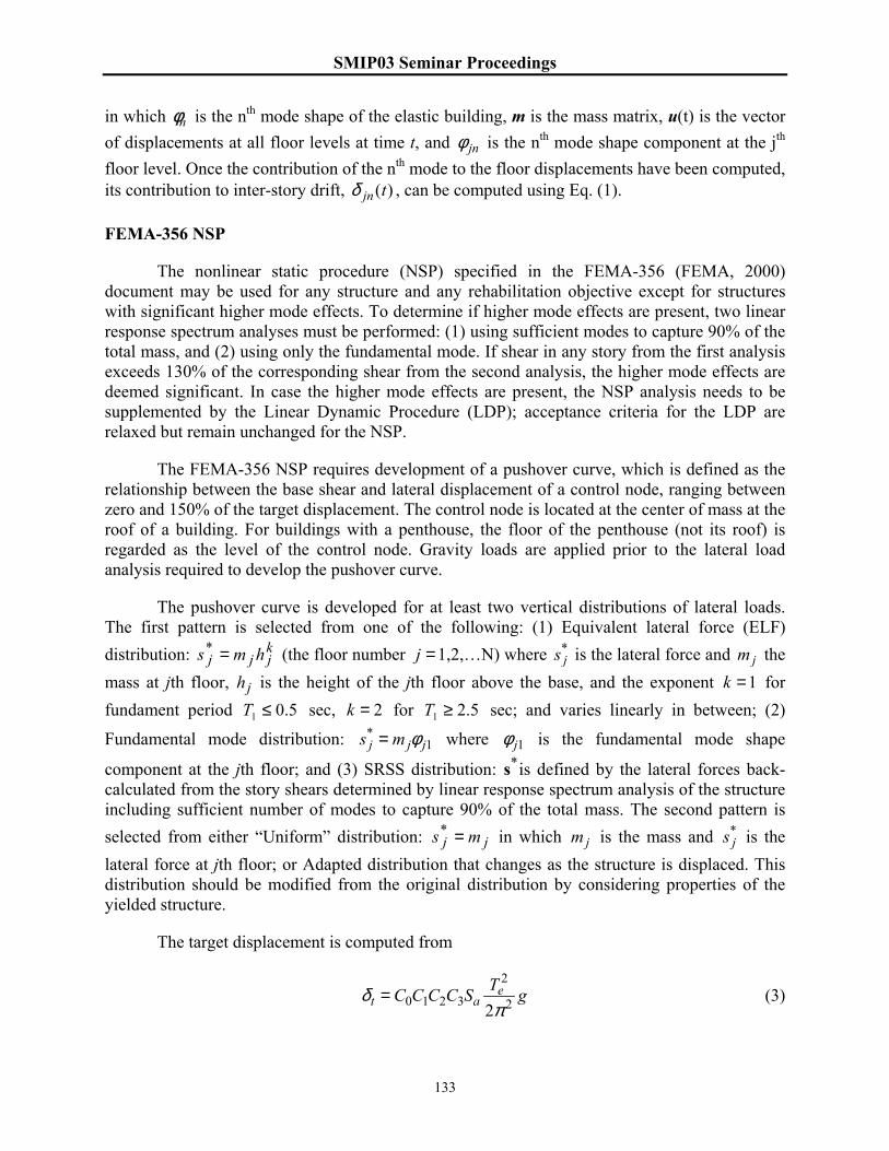
SMIP03 Seminar Proceedings
133
in which nφ is the nth mode shape of the elastic building, m is the mass matrix, u(t) is the vector of displacements at all floor levels at time t, and jnφ is the nth mode shape component at the jth
floor level. Once the contribution of the nth mode to the floor displacements have been computed, its contribution to inter-story drift, ( )jn tδ , can be computed using Eq. (1).
FEMA-356 NSP
The nonlinear static procedure (NSP) specified in the FEMA-356 (FEMA, 2000) document may be used for any structure and any rehabilitation objective except for structures with significant higher mode effects. To determine if higher mode effects are present, two linear response spectrum analyses must be performed: (1) using sufficient modes to capture 90% of the total mass, and (2) using only the fundamental mode. If shear in any story from the first analysis exceeds 130% of the corresponding shear from the second analysis, the higher mode effects are deemed significant. In case the higher mode effects are present, the NSP analysis needs to be supplemented by the Linear Dynamic Procedure (LDP); acceptance criteria for the LDP are relaxed but remain unchanged for the NSP.
The FEMA-356 NSP requires development of a pushover curve, which is defined as the relationship between the base shear and lateral displacement of a control node, ranging between zero and 150% of the target displacement. The control node is located at the center of mass at the roof of a building. For buildings with a penthouse, the floor of the penthouse (not its roof) is regarded as the level of the control node. Gravity loads are applied prior to the lateral load analysis required to develop the pushover curve.
The pushover curve is developed for at least two vertical distributions of lateral loads. The first pattern is selected from one of the following: (1) Equivalent lateral force (ELF) distribution: k
jjj hms =* (the floor number =j 1,2,…N) where *js is the lateral force and jm the
mass at jth floor, hj is the height of the jth floor above the base, and the exponent 1=k for fundament period 5.01 ≤T sec, 2=k for 5.21 ≥T sec; and varies linearly in between; (2)
Fundamental mode distribution: *1j j js m φ= where 1jφ is the fundamental mode shape
component at the jth floor; and (3) SRSS distribution: s*is defined by the lateral forces back-calculated from the story shears determined by linear response spectrum analysis of the structure including sufficient number of modes to capture 90% of the total mass. The second pattern is selected from either “Uniform” distribution: jj ms =* in which jm is the mass and *
js is the lateral force at jth floor; or Adapted distribution that changes as the structure is displaced. This distribution should be modified from the original distribution by considering properties of the yielded structure.
The target displacement is computed from
2
0 1 2 3 22e
t aTC C C C S gδπ
= (3)
SMIP03 Seminar Proceedings
134
where eT = Effective fundamental period of the building in the direction under consideration, aS = Response spectrum acceleration at the effective fundamental vibration period and damping ratio of the building under consideration and g is the acceleration due to gravity, 0C = Modification factor that relates the elastic response of an SDF system to the elastic displacement of the MDF building at the control node, 1C = Modification factor that relates the maximum inelastic and elastic displacement of the SDF system, 2C = Modification factor to represent the effects of pinched hysteretic shape, stiffness degradation, and strength deterioration, and 3C = Modification factor to represent increased displacement due to P-delta effects.
The deformation/force demands in each structural element is computed at the target displacement and compared against acceptability criteria set forth in the FEMA-356 document. These criteria depend on the material (e.g., concrete, steel), type of member (e.g., beam, column, panel zones, connections etc.), importance of the member (e.g., primary, secondary) and the structural performance levels (e.g., immediate occupancy, life safety, collapse prevention).
The FEMA-356 NSP procedure contains several approximations. These include those in estimating the target displacement from Eq. 3, and using the pushover curve to estimate the member demands imposed by the earthquake. In this investigation, the focus is primarily on the second source of approximation; the first approximation is a focus of numerous other investigations. For this purpose, the following analysis method is employed.
The target displacement is selected to be equal to that of the roof level recorded during the earthquake, as opposed to calculating it according to the FEMA-356 document (Eq. 3). The structure is pushed to this target displacement using the FEMA-356 lateral load patterns and inter-story drifts are computed. These computed inter-story drifts are then compared with the “derived” inter-story drifts, i.e., those computed directly from the recorded motions using the procedure described in the preceding section. Such an analysis enables evaluation of the adequacy of various lateral load patterns in the FEMA-356 NSP, in particular, if the FEMA-356 NSP is able to capture the higher mode effects, which are likely to be present in the selected buildings.
MPA Procedure
Recently a MPA procedure has been developed to account for the higher mode effects and analytically tested for SAC buildings and ground motions (Chopra and Goel, 2001, 2002). This procedure has been found to be highly accurate unless the building is deformed far into the region of stiffness and strength deterioration (Goel and Chopra, 2002). Following is a brief summary of this procedure.
1. Compute the natural frequencies, ωn and modes, nφ , for linearly elastic vibration of the building.
2. For the nth-mode, develop the base shear-roof displacement, rnbn uV − , pushover curve for
force distribution, nn ms φ=* , where m is the mass matrix of the structure. Gravity loads, including those present on the interior (gravity) frames, are applied before the first-“mode”

SMIP03 Seminar Proceedings
135
pushover analysis. The resulting P-delta effects may lead to negative post-yielding stiffness in the pushover curve. The gravity loads are not included in the higher-“mode” pushover curves.
3. Idealize the pushover curve as a bilinear curve. If the pushover curve exhibits negative post-yielding stiffness, the second stiffness (or post-yield stiffness) of the bilinear curve would be negative.
4. Convert the idealized bn rnV u− pushover curve to the force-displacement, nnsn DLF −/ , relation for the nth -“mode” inelastic SDF system by utilizing
* and sny n bny n ny rny n rnF L V M D u φ= = Γ in which Mn* is the effective modal mass, φrn is
the value of φn at the roof, and nTn
Tnn mm φφφ /1=Γ .
5. Compute the peak deformation Dn of the nth-“mode” inelastic single-degree-of-freedom (SDF) system defined by the force-deformation relation developed in Step 4 and damping
ratio ζ n. The elastic vibration period of the system is ( )1/ 22n n ny snyT L D Fπ= . For an SDF
system with known Tn , ζ n and a selected earthquake excitation, Dn can be computed by either by nonlinear RHA of the SDF system or from inelastic design spectrum.
6. Calculate peak roof displacement urn associated with the nth-“mode” inelastic SDF system from nrnnrn Du φΓ= .
7. From the pushover database (Step 2), extract values of desired responses rn : floor displacements, story drifts, plastic hinge rotations, etc.
8. Repeat Steps 3-7 for as many modes as required for sufficient accuracy. Typically, the first two or three “modes” will suffice.
9. Determine the total response (demand) by combining the peak “modal” responses using the
SRSS rule: 2/1
2
≈ ∑
nnrr .
Steps 3 to 6 of the MPA procedure described above are used to compute the peak roof displacement associated with the nth-“mode” inelastic SDF system. However, these steps are not necessary for analysis of a building for which recorded motions are available. The contribution of the nth-“mode” to the total roof displacement, rnu , can be computed from modal decomposition of recorded motion using Eq. (2).
In the MPA procedure, total floor displacements and story drifts can be computed within sufficient degree of accuracy by combining the values obtained from “modal” pushover analysis (Step 9). However, this procedure may not lead to accurate estimates of localized demands such as plastic rotations and member forces. For this purpose, improved procedure are being developed.
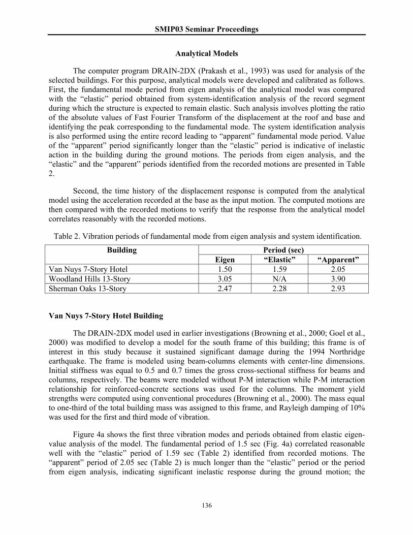
SMIP03 Seminar Proceedings
136
Analytical Models
The computer program DRAIN-2DX (Prakash et al., 1993) was used for analysis of the selected buildings. For this purpose, analytical models were developed and calibrated as follows. First, the fundamental mode period from eigen analysis of the analytical model was compared with the “elastic” period obtained from system-identification analysis of the record segment during which the structure is expected to remain elastic. Such analysis involves plotting the ratio of the absolute values of Fast Fourier Transform of the displacement at the roof and base and identifying the peak corresponding to the fundamental mode. The system identification analysis is also performed using the entire record leading to “apparent” fundamental mode period. Value of the “apparent” period significantly longer than the “elastic” period is indicative of inelastic action in the building during the ground motions. The periods from eigen analysis, and the “elastic” and the “apparent” periods identified from the recorded motions are presented in Table 2.
Second, the time history of the displacement response is computed from the analytical model using the acceleration recorded at the base as the input motion. The computed motions are then compared with the recorded motions to verify that the response from the analytical model correlates reasonably with the recorded motions.
Table 2. Vibration periods of fundamental mode from eigen analysis and system identification.
Period (sec) Building Eigen “Elastic” “Apparent”
Van Nuys 7-Story Hotel 1.50 1.59 2.05 Woodland Hills 13-Story 3.05 N/A 3.90 Sherman Oaks 13-Story 2.47 2.28 2.93
Van Nuys 7-Story Hotel Building
The DRAIN-2DX model used in earlier investigations (Browning et al., 2000; Goel et al., 2000) was modified to develop a model for the south frame of this building; this frame is of interest in this study because it sustained significant damage during the 1994 Northridge earthquake. The frame is modeled using beam-columns elements with center-line dimensions. Initial stiffness was equal to 0.5 and 0.7 times the gross cross-sectional stiffness for beams and columns, respectively. The beams were modeled without P-M interaction while P-M interaction relationship for reinforced-concrete sections was used for the columns. The moment yield strengths were computed using conventional procedures (Browning et al., 2000). The mass equal to one-third of the total building mass was assigned to this frame, and Rayleigh damping of 10% was used for the first and third mode of vibration.
Figure 4a shows the first three vibration modes and periods obtained from elastic eigen-value analysis of the model. The fundamental period of 1.5 sec (Fig. 4a) correlated reasonable well with the “elastic” period of 1.59 sec (Table 2) identified from recorded motions. The “apparent” period of 2.05 sec (Table 2) is much longer than the “elastic” period or the period from eigen analysis, indicating significant inelastic response during the ground motion; the
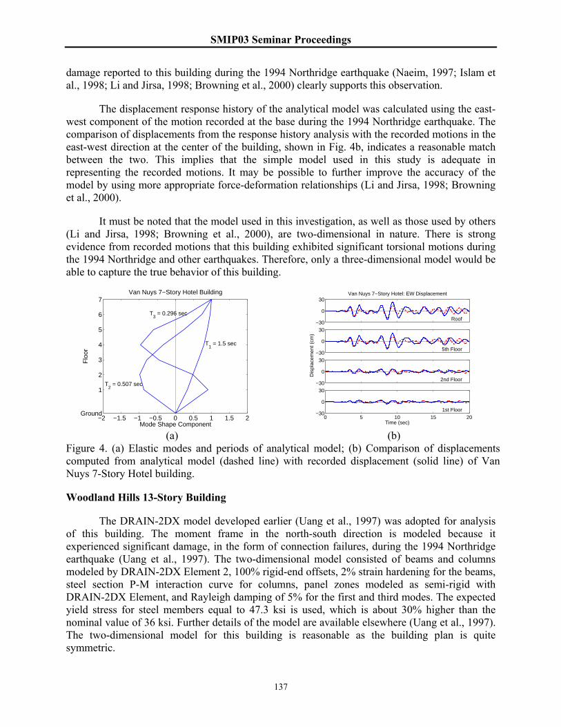
SMIP03 Seminar Proceedings
137
damage reported to this building during the 1994 Northridge earthquake (Naeim, 1997; Islam et al., 1998; Li and Jirsa, 1998; Browning et al., 2000) clearly supports this observation.
The displacement response history of the analytical model was calculated using the east-west component of the motion recorded at the base during the 1994 Northridge earthquake. The comparison of displacements from the response history analysis with the recorded motions in the east-west direction at the center of the building, shown in Fig. 4b, indicates a reasonable match between the two. This implies that the simple model used in this study is adequate in representing the recorded motions. It may be possible to further improve the accuracy of the model by using more appropriate force-deformation relationships (Li and Jirsa, 1998; Browning et al., 2000).
It must be noted that the model used in this investigation, as well as those used by others (Li and Jirsa, 1998; Browning et al., 2000), are two-dimensional in nature. There is strong evidence from recorded motions that this building exhibited significant torsional motions during the 1994 Northridge and other earthquakes. Therefore, only a three-dimensional model would be able to capture the true behavior of this building.
−2 −1.5 −1 −0.5 0 0.5 1 1.5 2Mode Shape Component
Van Nuys 7−Story Hotel Building
Flo
or
Ground
1
2
3
4
5
6
7
T1 = 1.5 sec
T2 = 0.507 sec
T3 = 0.296 sec
(a)
−30
0
30Van Nuys 7−Story Hotel: EW Displacement
Roof
−30
0
30
Dis
plac
emen
t (cm
)
5th Floor
−30
0
30
2nd Floor
0 5 10 15 20−30
0
30
Time (sec)
1st Floor
(b)
Figure 4. (a) Elastic modes and periods of analytical model; (b) Comparison of displacements computed from analytical model (dashed line) with recorded displacement (solid line) of Van Nuys 7-Story Hotel building.
Woodland Hills 13-Story Building
The DRAIN-2DX model developed earlier (Uang et al., 1997) was adopted for analysis of this building. The moment frame in the north-south direction is modeled because it experienced significant damage, in the form of connection failures, during the 1994 Northridge earthquake (Uang et al., 1997). The two-dimensional model consisted of beams and columns modeled by DRAIN-2DX Element 2, 100% rigid-end offsets, 2% strain hardening for the beams, steel section P-M interaction curve for columns, panel zones modeled as semi-rigid with DRAIN-2DX Element, and Rayleigh damping of 5% for the first and third modes. The expected yield stress for steel members equal to 47.3 ksi is used, which is about 30% higher than the nominal value of 36 ksi. Further details of the model are available elsewhere (Uang et al., 1997). The two-dimensional model for this building is reasonable as the building plan is quite symmetric.

SMIP03 Seminar Proceedings
138
The displacement response of above described model computed to the north-south component of the motions recorded at the base matched reasonably well with the recorded motions in this direction (Uang et al., 1997). However, when this model is pushed during the pushover analysis (presented later in this paper) to the peak roof displacement recorded during the 1994 Northridge earthquake, none of its elements yield. This behavior of the model is contrary to the physical observation during the post-earthquake inspection, which revealed numerous beam-column connection failures. Therefore, the model was modified by reducing the strengths of beams and panel zone elements by 25% compared to the original model. This brings the expected yield stress close to the nominal yield stress of 36 ksi. Furthermore, the Rayleigh damping was increased from 5% to 7% in the first and third modes.
−1.5 −1 −0.5 0 0.5 1 1.5Mode Shape Component
Woodland Hills 13−Story Building
Flo
or
GroundPlaza
123456789
101112
Roof
T1 = 3.05 sec
T2 = 1.06 sec
T3 = 0.63 sec
(a)
0 5 10 15 20 25 30−50
−25
0
25
50
Dis
p. (
cm)
Woodland Hills 13−Story Building: NS Displacements
12th Floor
0 5 10 15 20 25 30−30
−15
0
15
30
Time (sec)
Dis
p. (
cm)
6th Floor
(b)
Figure 5. (a) Elastic modes and periods of analytical model; (b) Comparison of displacements computed from analytical model (dashed line) with recorded displacement (solid line) of Woodland Hills 13-Story building.
The fundamental period of this building from the eigen analysis is 3.05 sec (Fig. 5a). The system identification could not identify the true “elastic” period for this building because long-enough initial time segment of the recorded motions during which the building behaved elastically could not be selected. The “apparent” period of 3.9 sec (Table 2) is much longer than the period from eigen analysis, indicating inelastic response during the ground motion; the damage reported to this building during the 1994 Northridge earthquake (Uang et al., 1997) clearly supports this observation.
The displacement response history of the analytical model was calculated using the north-south component of the motion recorded at the base during the 1994 Northridge earthquake. The comparison of displacements from the response history analysis with the recorded motions in the north-south direction at the center of the building, shown in Fig. 5b, indicates a reasonable match between the two. This implies that the simple model used in this study is adequate in representing the recorded motions. It may be possible to further improve the accuracy of the model by using more appropriate connection behavior.
Sherman Oaks 13-Story Commercial Building
The DRAIN-2DX model was developed for the exterior frame in the east-west direction for this building. The model was developed based on the structural plans and additional

SMIP03 Seminar Proceedings
139
information available in an earlier study (John A. Martin & Associates, 1973). The frame is modeled using beam-columns elements with center-line dimensions. Initial stiffness was equal to 0.5 and 0.7 times the gross cross-sectional stiffness for beams and columns respectively. Rigid end offsets equal to 50% of the joint dimensions were assumed. The beams were modeled without P-M interaction while P-M interaction relationship for reinforced-concrete sections was used for the columns. The moment yield strengths were computed using moment-curvature analysis. The nominal strength of beams were increased by 25% for a better match with the recorded motions. The mass equal to one-third of the total building mass was assigned to this frame, and Rayleigh damping of 10% was assigned to the first and third mode of vibration.
−1.5 −1 −0.5 0 0.5 1 1.5Mode Shape Component
Sherman Oaks 13−Story Commercial Building
Flo
or
2nd Sub1st Sub
1
23456789
10111213
Roof
Roof1
T1 = 2.47 sec
T2 = 0.798 sec
T3 = 0.456 sec
−40
−20
0
20
40Sherman Oaks 13−Story Commercial Building
Roof
−30
−15
0
15
30
Dis
p. (
cm)
8th Floor
0 5 10 15 20 25 30−10
−5
0
5
10
Time (sec)
2nd Floor
Figure 6. (a) Elastic modes and periods of analytical model; (b) Comparison of displacements computed from analytical model (dashed line) with recorded displacement (solid line) of Sherman Oaks 13-Story Commercial building.
Figure 6a shows the first three vibration modes and periods obtained from elastic eigen-value analysis of the model. The fundamental period of 2.47 sec (Fig. 6a) is slightly longer than the “elastic” period of 2.28 sec (Table 2) identified from recorded motions. The “apparent” period of 2.93 sec (Table 2) is much longer than the “elastic” period or the period from eigen analysis, indicating some inelastic response during the ground motion; the post earthquake investigation indicates minor cracking at the beam columns joints after the 1994 Northridge earthquake (Naeim, 1997).
The displacement response history of the analytical model was calculated using the east-west component of the motion recorded at the base during the 1994 Northridge earthquake. The comparison of displacements from the response history analysis with the recorded motions in the east-west direction at the center of the building, shown in Fig. 6b, indicates a reasonable match between the two. This implies that the simple model used in this study is reasonable in representing the recorded motions. As mentioned previously for the Van Nuys building, it may be possible to further improve the accuracy of the model by using more appropriate force-deformation relationships.
Evaluation of Nonlinear Static Procedures
The FEMA-356 NSP and MPA procedures are evaluated in this section using recorded motions of selected buildings. Presented for each selected buildings are the pushover curves for the four FEMA-356 distributions for the FEMA NSP analysis and the first three “modes” for the
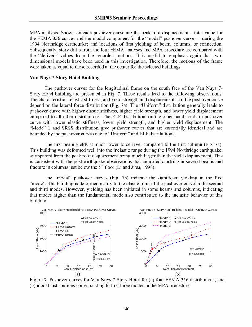
SMIP03 Seminar Proceedings
140
MPA analysis. Shown on each pushover curve are the peak roof displacement – total value for the FEMA-356 curves and the modal component for the “modal” pushover curves – during the 1994 Northridge earthquake; and locations of first yielding of beam, columns, or connection. Subsequently, story drifts from the four FEMA analyses and MPA procedure are compared with the “derived” values from the recorded motions. It is useful to emphasis again that two-dimensional models have been used in this investigation. Therefore, the motions of the frame were taken as equal to those recorded at the center for the selected buildings.
Van Nuys 7-Story Hotel Building
The pushover curves for the longitudinal frame on the south face of the Van Nuys 7-Story Hotel building are presented in Fig. 7. These results lead to the following observations. The characteristic – elastic stiffness, and yield strength and displacement – of the pushover curve depend on the lateral force distribution (Fig. 7a). The “Uniform” distribution generally leads to pushover curve with higher elastic stiffness, higher yield strength, and lower yield displacement compared to all other distributions. The ELF distribution, on the other hand, leads to pushover curve with lower elastic stiffness, lower yield strength, and higher yield displacement. The “Mode” 1 and SRSS distribution give pushover curves that are essentially identical and are bounded by the pushover curves due to “Uniform” and ELF distributions.
The first beam yields at much lower force level compared to the first column (Fig. 7a). This building was deformed well into the inelastic range during the 1994 Northridge earthquake, as apparent from the peak roof displacement being much larger than the yield displacement. This is consistent with the post-earthquake observations that indicated cracking in several beams and fracture in columns just below the 5th floor (Li and Jirsa, 1998).
The “modal” pushover curves (Fig. 7b) indicate the significant yielding in the first “mode”. The building is deformed nearly to the elastic limit of the pushover curve in the second and third modes. However, yielding has been initiated in some beams and columns, indicating that modes higher than the fundamental mode also contributed to the inelastic behavior of this building.
0 5 10 15 20 25 300
1000
2000
3000
4000
Roof Displacement (cm)
Bas
e S
hear
(kN
)
Van Nuys 7−Story Hotel Building: FEMA Pushover Curves
W = 13691 kN
H = 2002.8 cm
"Mode" 1FEMA UniformFEMA ELFFEMA SRSS
Pea
k R
oof D
isp.
= 2
1.3
cm
First Beam Yields
First Column Yields
(a)
0 5 10 15 20 25 300
1000
2000
3000
4000
Roof Displacement (cm)
Bas
e S
hear
(kN
)
Van Nuys 7−Story Hotel Building: "Modal" Pushover Curves
W = 13691 kN
H = 2002.8 cm
"Mode" 1
21.1
"Mode" 2
2.93
"Mode" 3
2.75
First Beam Yields
First Column Yields
(b)
Figure 7. Pushover curves for Van Nuys 7-Story Hotel for (a) four FEMA-356 distributions; and (b) modal distributions corresponding to first three modes in the MPA procedure.
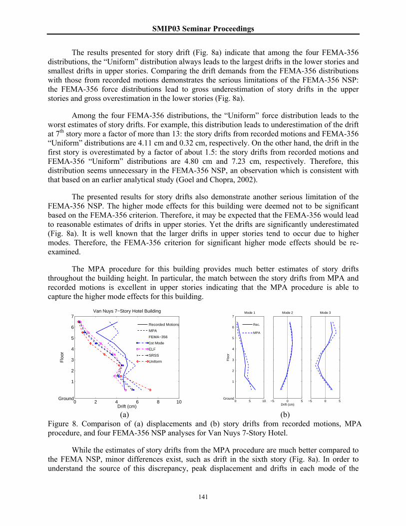
SMIP03 Seminar Proceedings
141
The results presented for story drift (Fig. 8a) indicate that among the four FEMA-356 distributions, the “Uniform” distribution always leads to the largest drifts in the lower stories and smallest drifts in upper stories. Comparing the drift demands from the FEMA-356 distributions with those from recorded motions demonstrates the serious limitations of the FEMA-356 NSP: the FEMA-356 force distributions lead to gross underestimation of story drifts in the upper stories and gross overestimation in the lower stories (Fig. 8a).
Among the four FEMA-356 distributions, the “Uniform” force distribution leads to the worst estimates of story drifts. For example, this distribution leads to underestimation of the drift at 7th story more a factor of more than 13: the story drifts from recorded motions and FEMA-356 “Uniform” distributions are 4.11 cm and 0.32 cm, respectively. On the other hand, the drift in the first story is overestimated by a factor of about 1.5: the story drifts from recorded motions and FEMA-356 “Uniform” distributions are 4.80 cm and 7.23 cm, respectively. Therefore, this distribution seems unnecessary in the FEMA-356 NSP, an observation which is consistent with that based on an earlier analytical study (Goel and Chopra, 2002).
The presented results for story drifts also demonstrate another serious limitation of the FEMA-356 NSP. The higher mode effects for this building were deemed not to be significant based on the FEMA-356 criterion. Therefore, it may be expected that the FEMA-356 would lead to reasonable estimates of drifts in upper stories. Yet the drifts are significantly underestimated (Fig. 8a). It is well known that the larger drifts in upper stories tend to occur due to higher modes. Therefore, the FEMA-356 criterion for significant higher mode effects should be re-examined.
The MPA procedure for this building provides much better estimates of story drifts throughout the building height. In particular, the match between the story drifts from MPA and recorded motions is excellent in upper stories indicating that the MPA procedure is able to capture the higher mode effects for this building.
0 2 4 6 8 10Drift (cm)
Van Nuys 7−Story Hotel Building
Flo
or
Ground
1
2
3
4
5
6
7
Recorded Motions
MPA
FEMA−356
1st Mode
ELF
SRSS
Uniform
(a)
0 5 10
Mode 1
Flo
or
Ground
1
2
3
4
5
6
7
Rec.
MPA
−5 0 5
Mode 2
Drift (cm)−5 0 5
Mode 3
(b)
Figure 8. Comparison of (a) displacements and (b) story drifts from recorded motions, MPA procedure, and four FEMA-356 NSP analyses for Van Nuys 7-Story Hotel.
While the estimates of story drifts from the MPA procedure are much better compared to the FEMA NSP, minor differences exist, such as drift in the sixth story (Fig. 8a). In order to understand the source of this discrepancy, peak displacement and drifts in each mode of the

SMIP03 Seminar Proceedings
142
MPA procedure are compared with those obtained from modal decomposition of recorded motions (Fig. 8b). This comparison shows that the match between the two is reasonably good. Therefore, the prime source of discrepancy appears to be from modal combination procedure. The modal combination rule was found to be deficient in an earlier study (Goel and Chopra, 2002) even for elastic buildings. Furthermore, the SRSS combination rule is likely to be inaccurate for individual ground motion as it was developed to work well with smooth design spectrum. The research is currently underway by others to develop improved modal combination rules. With improved modal combination rules, the accuracy of the MPA procedure may be expected to further improve.
Woodland Hills 13-Story Building
The pushover curves for the longitudinal frame on in the north-south direction of the Woodland Hills 13-Story building are presented in Fig. 9. These results lead to the following observations. The characteristic – elastic stiffness, yield strength and displacement, and post-yield strength decay – of the pushover curve depend on the lateral force distribution (Fig. 9a). The “Uniform” distribution generally leads to pushover curve with higher elastic stiffness, higher yield strength, lower yield displacement, and more rapid decay in post-yield strength compared to all other distributions. The ELF distribution, on the other hand, leads to pushover curve with lower elastic stiffness, lower yield strength, and higher yield displacement. The “Mode” 1 and SRSS distribution give pushover curves that are essentially identical up to the elastic limit. Thereafter, the strength is higher for the SRSS distribution compared to the “Mode” 1 distribution. The first yielding occurs in the connection followed soon after by the first yielding of the beam (Fig. 9a). The columns yielding occurs at much higher deformation level and is soon followed by rapid decay in the strength. This building is deformed only slightly beyond the elastic limit during the 1994 Northridge earthquake. The “modal” pushover curves (Fig. 9b) also indicate the slight yielding in the first “mode”. The building remains elastic in all higher modes.
0 25 50 75 100 125 1500
2000
4000
6000
8000
10000
Roof Displacement (cm)
Bas
e S
hear
(kN
)
Woodland Hills 12−Story Building: FEMA Pushover Curves
W = 70007 kNH = 5745.5 cm
"Mode" 1FEMA UniformFEMA ELFFEMA SRSS
NS
Roo
f Dis
p. =
34
cm
Yielding of 1stBeamColumnConnection
(a)
0 25 50 75 100 125 1500
2000
4000
6000
8000
10000
Roof Displacement (cm)
Bas
e S
hear
(kN
)
Woodland Hills 13−Story Building: "Modal" Pushover Curves
W = 70007 kNH = 5745.5 cm
"Mode" 1
36.3
"Mode" 24.81 "Mode" 3
4.14
Yielding of 1stBeamColumnConnection
(b)
Figure 9. Pushover curves of Woodland Hills 13-Story building for: (a) four FEMA-356 distributions; and (b) modal distributions corresponding to first three modes in the MPA procedure.
The results presented for story drift (Fig. 10a) indicate that the FEMA-356 distributions provide reasonable estimates at lower stories. However, the FEMA-356 force distributions lead to gross underestimation of story drifts in the upper stories (Fig. 10a). As noted earlier, among

SMIP03 Seminar Proceedings
143
the four FEMA-356 distributions, the “Uniform” force distribution leads to the worst estimates of story drifts. For example, this distribution leads to underestimation of the drift at 12th story more a factor of about 3: the story drifts from recorded motions and FEMA-356 “Uniform” distributions are 3.01 cm and 1.02 cm, respectively.
It must be noted that higher mode effects are likely to be significant for this building. Therefore, the higher drifts noted in upper stories from the recorded motions are due to higher modes. Clearly, FEMA-356 distributions are unable to adequately represent the drifts in upper stories due to higher modes.
0 2 4 6 8 10Drift (cm)
Woodland Hills 13−Story Building
Flo
or
GroundPlaza
123456789
101112
Roof
Recorded Motions
MPA
FEMA−356
1st Mode
ELF
SRSS
Uniform
(a)
0 5
Mode 1
Flo
orGround
Plaza
1
2
3
4
5
6
7
8
9
10
11
12
Roof
Rec.MPA
−2 0 2
Mode 2
−5 0 5
Mode 3
Drift (cm)−1 0 1
Mode 4
−2 0 2
Mode 5
(b)
Figure 10. Comparison of (a) displacements and (b) story drifts from recorded motions, MPA procedure, and four FEMA-356 NSP analyses for Woodland Hills 13-Story building.
The MPA procedure for this building in general provides excellent estimates of the story drifts (Fig. 10a), except for the 13th story, indicating that the MPA procedure is able to capture the effects of higher modes. The comparison of drifts from MPA and those from modal decomposition of recorded motions for each mode (Fig. 10b) shows an excellent match between the two. Therefore, the slight discrepancy between the results from MPA and recorded motions are due to the modal combination procedure, which are likely to be inaccurate for individual ground motions. With improved modal combination rules, the accuracy of the MPA procedure may be expected to further improve.
Sherman Oaks 13-Story Commercial Building
The pushover curves for the longitudinal frame on in the east-west direction of the Sherman Oaks 13-Story building are presented in Fig. 11. As noted previously, the characteristic – elastic stiffness, yield strength and displacement, and post-yield strength decay – of the pushover curve depend on the lateral force distribution (Fig. 11a). The “Uniform” distribution generally leads to pushover curve with higher elastic stiffness, higher yield strength, lower yield displacement, and more rapid decay in post-yield strength compared to all other distributions. The ELF distribution, on the other hand, leads to pushover curve with lower elastic stiffness, lower yield strength, and higher yield displacement. The “Mode” 1 and SRSS distribution give pushover curves that are essentially identical and bounded by the “Uniform” and ELF curves. The first yielding occurs in the beam followed soon after by the first yielding of the column (Fig. 11a). This building is deformed significantly beyond the elastic limit during the 1994 Northridge
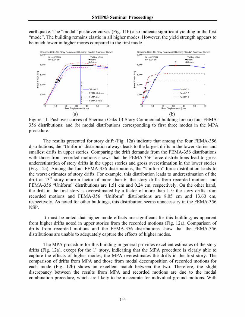
SMIP03 Seminar Proceedings
144
earthquake. The “modal” pushover curves (Fig. 11b) also indicate significant yielding in the first “mode”. The building remains elastic in all higher modes. However, the yield strength appears to be much lower in higher mores compared to the first mode.
0 10 20 30 40 50 600
1000
2000
3000
4000
5000
Roof Displacement (cm)
Bas
e S
hear
(kN
)
Sherman Oaks 13−Story Commercial Building: "Modal" Pushover Curves
W = 40727 kNH = 5014 cm
"Mode" 1
FEMA Uniform
FEMA ELF
FEMA SRSS
EW
Roo
f Dis
p. =
33.
6 cm
Yielding of 1stBeamColumn
(a)
0 10 20 30 40 50 600
1000
2000
3000
4000
5000
Roof Displacement (cm)
Bas
e S
hear
(kN
)
Sherman Oaks 13−Story Commercial Building: "Modal" Pushover Curves
W = 40727 kNH = 5014 cm
"Mode" 1
32
"Mode" 22.59
"Mode" 30.898
Yielding of 1stBeamColumn
(b)
Figure 11. Pushover curves of Sherman Oaks 13-Story Commercial building for: (a) four FEMA-356 distributions; and (b) modal distributions corresponding to first three modes in the MPA procedure.
The results presented for story drift (Fig. 12a) indicate that among the four FEMA-356 distributions, the “Uniform” distribution always leads to the largest drifts in the lower stories and smallest drifts in upper stories. Comparing the drift demands from the FEMA-356 distributions with those from recorded motions shows that the FEMA-356 force distributions lead to gross underestimation of story drifts in the upper stories and gross overestimation in the lower stories (Fig. 12a). Among the four FEMA-356 distributions, the “Uniform” force distribution leads to the worst estimates of story drifts. For example, this distribution leads to underestimation of the drift at 13th story more a factor of more than 6: the story drifts from recorded motions and FEMA-356 “Uniform” distributions are 1.51 cm and 0.24 cm, respectively. On the other hand, the drift in the first story is overestimated by a factor of more than 1.5: the story drifts from recorded motions and FEMA-356 “Uniform” distributions are 8.05 cm and 13.60 cm, respectively. As noted for other buildings, this distribution seems unnecessary in the FEMA-356 NSP.
It must be noted that higher mode effects are significant for this building, as apparent from higher drifts noted in upper stories from the recorded motions (Fig. 12a). Comparison of drifts from recorded motions and the FEMA-356 distributions show that the FEMA-356 distributions are unable to adequately capture the effects of higher modes.
The MPA procedure for this building in general provides excellent estimates of the story drifts (Fig. 12a), except for the 1st story, indicating that the MPA procedure is clearly able to capture the effects of higher modes; the MPA overestimates the drifts in the first story. The comparison of drifts from MPA and those from modal decomposition of recorded motions for each mode (Fig. 12b) shows an excellent match between the two. Therefore, the slight discrepancy between the results from MPA and recorded motions are due to the modal combination procedure, which are likely to be inaccurate for individual ground motions. With

SMIP03 Seminar Proceedings
145
improved modal combination rules, the accuracy of the MPA procedure may be expected to further improve.
0 3 6 9 12 15Drift (cm)
Sherman Oaks 13−Story Commercial Building
Flo
or
2S 1
3 5 7 9
11
13R
R1
Recorded Motions
MPA
FEMA−356
1st Mode
ELF
SRSS
Uniform
(a)
0 10 20
Mode 1
Flo
or
2S
1
3
5
7
9
11
13R
R1
Rec.MPA
−5 0 5
Mode 2
−1 0 1
Mode 3
Drift (cm)−2 0 2
Mode 4
−2 0 2
Mode 5
(b)
Figure 12. Comparison of (a) displacements and (b) story drifts from recorded motions, MPA procedure, and four FEMA-356 NSP analyses for Sherman Oaks 13-Story Commercial building.
Conclusions
This research investigation on evaluation of the FEMA-356 NSP and MPA procedure using recorded motions of buildings that were damaged during the 1994 Northridge earthquake has led to the following conclusions.
1. The FEMA-356 NSP leads to significant underestimation of drifts in upper stories of the selected buildings. The underestimation ranges by a factor of 13 for the Van Nuys building to 3 for the Sherman Oaks building.
2. The FEMA-356 NSP is unable to account for higher mode effects, which typical contribute significantly to the drifts in upper stories.
3. The FEMA-356 NSP leads to significant overestimation – by a factor of 1.5 – of drift in lower stories for Van Nuys and Sherman Oaks buildings.
4. Among the four FEMA-356 distributions, the “Uniform” force distribution leads to the most excessive underestimation in upper stories and overestimation in the lower stories. Therefore, this distribution seems unnecessary in the FEMA-356 NSP.
5. The FEMA-356 NSP is expected to provide reasonable estimate of the response if the higher mode effects are deemed not to be significant based on the FEMA-356 criterion. Although the FEMA-356 criterion is satisfied for the Van Nuys building, the drifts in upper stories are significantly underestimated indicating the need to re-examine the FEMA-356 criterion for evaluating significant higher mode effects.
6. The MPA procedure provides much better estimates of drifts compared to the FEMA-356 NSP, and is able to account for the higher mode effects.
7. The response for each mode in the MPA procedure matched closely with the modal response obtained from decomposition of the recorded motions, indicating the observed discrepancy between the response from MPA and recorded response is due to limitations in the
SMIP03 Seminar Proceedings
146
combination procedure. With development of the improved combination procedures, accuracy of the MPA procedure is likely to improve.
Acknowledgment
This research investigation is supported by the California Department of Conservation, California Geological Survey, Strong Motion Instrumentation Program (SMIP) through Contract No. 1001-762. This support is gratefully acknowledged. The author is grateful to Dr. Moh Huang and Mr. David Whitesel of SMIP for providing the recorded motions and structural plans of the selected buildings. Also acknowledged is the assistance provided by Dr. Abe Lynn of Cal Poly, San Luis Obispo, and Dr. Kent Yu of Degenkolb Engineers; the analytical model for the Van Nuys and Woodland Hills buildings were developed from those provided by Dr. Lynn and Dr. Yu, respectively.
References
Bracci, J. M., Kunnath, S. K. and Reinhorn, A. M. (1997). Seismic Performance and Retrofit Evaluation for Reinforced Concrete Structures, Journal of Structural Engineering, ASCE, 123(1): 3-10.
Browning, J., Li, Y. R., Lynn, A. C. and Moehle, J. P. (2000). Performance Assessment for a Reinforced Concrete Frame Building, Earthquake Spectra, 16(3): 541-555.
Chopra, A. K. (2001). Dynamics of Structures: Theory and Application to Earthquake Engineering, Prentice Hall, New Jersey.
Chopra, A. K. and Goel, R. K. (2001). A Modal Pushover Analysis Procedure to Estimate Seismic Demands for Buildings: Theory and Preliminary Evaluation, Report No. PEER 2001/03, Pacific Earthquake Engineering Research Center, University of California, Berkeley, CA.
Chopra, A. K. and Goel, R. K. (2002). A Modal Pushover Analysis Procedure for Estimating Seismic Demands for Buildings, Earthquake Engineering and Structural Dynamics, 31: 561-582.
Darragh, R. B., Cao, T., Graizer, V., Shakal, A. and Huang, M. (1994). Los Angeles Code-Instrumented Building Records from the Northridge, California Earthquake of January 17, 1994: Processed Release No. 1, Report No. OSMS 94-17, Strong Motion Instrumentation Program, CDMG.
De la Llera, J. C. and Chopra, A. K. (1998). Evaluation of Seismic Code Provisions Using Strong-Motion Building Records from the 1994 Northridge Earthquake, Report No. UCB/EERC-97/16, Earthquake Engineering Research Center, University of California, Berkeley, CA.
Fajfar, P. and Gaspersic, P. (1996). The N2 Method for the Seismic Damage Analysis of RC Buildings, Earthquake Engineering and Structural Dynamics, 25(1): 31-46.
FEMA (1997). NEHRP Commentary on the Guidelines for the Seismic Rehabilitation of Buildings, Report No. FEMA-274, Building Seismic Safety Council, Federal Emergency Management Agency, Washington, D.C.

SMIP03 Seminar Proceedings
147
FEMA (2000). Prestandard and Commentary for the Seismic Rehabilitation of Buildings, Report No. FEMA-356, Building Seismic Safety Council, Federal Emergency Management Agency, Washington, D.C.
Goel, R. K. and Chopra, A. K. (2002). Evaluation of Modal and FEMA Pushover Analyses Using SAC Buildings, Earthquake Spectra, Submitted for Publication.
Goel, R. K., Lynn, A. C., May, V. V., Rihal, S. S. and Weggel, D. (2000). Evaluating Current Procedures and Modeling for Seismic Performance of Reinforced Concrete Buildings, Proceedings, 12th World Conference on Earthquake Engineering, Paper No. 2060, Auckland, New Zealand.
Gupta, A. and Krawinkler, H. (1999). Seismic Demands for Performance Evaluation of Steel Moment Resisting Frame Structures (SAC Task 5.4.3), Report No. 132, John A. Blume Earthquake Engineering Center, Stanford, CA.
Gupta, B. and Kunnath, S. K. (2000). Adaptive Spectra-Based Pushover Procedure for Seismic Evaluation of Structures, Earthquake Spectra, 16(2): 367-392.
Islam, M. S., Gupta, B. and Kunnath, S. K. (1998). A Critical Review of State-of-Art Analytical Tools and Acceptance Criterion in Light of Observed Response of an Instrumented Nonductile Concrete Frame Building, Proceedings, 6th U.S. National Conference on Earthquake Engineering, Seattle, WA.
John A. Martin & Associates (1973). High-Rise Buildings -- Not Instrumented Union Bank, San Fernando, California, Earthquake of February 9, 1971, N. A. Benfer and J. L. Coffman (Eds.), U.S. Department of Commerce and National Oceanic and Atmospheric Administration, I of III: 629-638.
Krawinkler, H. and Seneviratna, G. (1998). Pros and Cons of a Pushover Analysis of Seismic Performance Evaluation, Engineering Structures, 20(4-6): 452-464.
Kunnath, S. K. and Gupta, B. (2000). Validity of Deformation Demand Estimates Using Nonlinear Static Procedures, Proceedings, U. S. Japan Workshop on Performance-Based Engineering for Reinforced Concrete Building Structures, Sapporo, Hokkaido, Japan.
Li, R. and Jirsa, J. O. (1998). Nonlinear Analysis of an Instrumented Structure Damaged in the 1994 Northridge Earthquake, Earthquake Spectra, 14(2): 265-283.
Maison, B. and Bonowitz, D. (1999). How Safe Are Pre-Northridge WSMFs? A Case Study of the Sac Los Angeles Nine-Story Building, Earthquake Spectra, 15(4): 765-789.
Matsumori, T., Otani, S., Shinohara, H. and Kabeyasawa, T. (1999). Earthquake Member Deformation Demands in Reinforced Concrete Frame Structures, Proceedings, U.S. Japan Workshop on Performance-Based Earthquake Engineering Methodology for RC Building Structures, 79-94, Maui, Hawaii.
Naeim, F. (1997). Performance of Extensively Instrumented Buildings During the January 17, 1994 Northridge Earthquake: An Interactive Information System, Report No. 97-7530.68, John A. Martin & Associates, Los Angeles, CA.
Naeim, F. (2000). Learning from Structural and Nonstructural Seismic Performance of 20 Extensively Instrumented Buildings, Proceedings, 12th World Conference on Earthquake Engineering, Paper No. 0217, Auckland, New Zealand.

SMIP03 Seminar Proceedings
148
Paret, T. F., Sasaki, K. K., Eilbeck, D. H. and Freeman, S. A. (1996). Approximate Inelastic Procedures to Identify Failure Mechanisms from Higher Mode Effects, Proceedings, 11th World Conference on Earthquake Engineering, Paper No. 966, Acapulco, Mexico.
Prakash, V., Powell, G. H. and Campbell, S. (1993). Drain-2DX Base Program Description and User Guide, Version 1.10, Report No. UCB/SEMM-93-17, Department of Civil Engineering, University of California, Berkeley, CA.
Sasaki, K. K., Freeman, S. A. and Paret, T. F. (1998). Multimode Pushover Procedure (MMP) - a Method to Identify the Effects of Higher Modes in a Pushover Analysis, Proceedings, 6th U.S. National Conference on Earthquake Engineering, Seattle, WA.
Shakal, A. F., Huang, M. and Darragh, R. B. (1994). Some Implications of Strong-Motion Records from the 1994 Northridge Earthquake, Proceedings, SMIP94 Seminar on Utilization of Strong-Motion Data, Strong Motion Instrumentation Program, CDMG, 1-20, Sacramento, CA.
Skokan, M. J. and Hart, G. C. (2000). Reliability of Nonlinear Static Methods for the Seismic Performance Prediction of Steel Frame Buildings, Proceedings, 12th World Conference on Earthquake Engineering, Paper No. 1972, Auckland, New Zealand.
Uang, C. M., Yu, Q. S., Sadre, A., Youssef, N. and Vinkler, J. (1997). Seismic Response of an Instrumented 13-Story Steel Frame Building Damaged in the 1994 Northridge Earthquake, Earthquake Spectra, 13(1): 131-149.
SMIP03 Seminar Proceedings
149
THE SEISMIC RETROFIT OF THE OAKLAND CITY HALL
Mason Walters, S.E., Principal
Forell/Elsesser Engineers, Inc. San Francisco, California
Abstract
The historic Oakland City Hall experienced extensive damage in the 1989 Loma Prieta earthquake, and was subsequently the focus of an intensive process of testing, historic evaluation, dynamic structural analysis, and retrofit design using seismic isolation. A comprehensive post-earthquake study done by a team of architects and engineers, and reviewed by FEMA and SHPO, concluded that seismic isolation was the most cost-effective and behavior-effective method to protect the landmark building and its occupants from seismic hazards. The retrofit was completed in 1995. Numerous technical challenges and questions were confronted in the course of this pioneering project. The resolution of these issues, and the features of the seismic design and analysis are discussed.
Introduction
The Oakland City Hall, completed in 1914, was the first high rise government office building in the United States and is listed in the National Register of Historic Places. The primary innovation of the original design was the “stacking” of building segments, each representing a distinct occupancy or function, one atop the other. Such a design with its significant height and numerous setbacks was possible due to the advent of the use of structural steel in building frames. The building was heavily damaged during the Loma Prieta earthquake in October, 1989. Approximately 20% of the building’s lateral strength was lost in the north-south direction, and 30% in the east-west direction, primarily due to extensive cracking of the numerous interior hollow clay tile partitions in the office tower. The clocktower at the top of the building “rocked” during the earthquake, resulting in large X cracks in some infill masonry walls and severe damage to several support transfer girders supporting the building’s clocktower.
The top of the 18-story building is 324 feet above street level. The structure sits atop a full basement. The lowest and widest portion of the building, known as the podium, is 3 stories tall and contains a central rotunda, council chambers, and administration offices of the Mayor and City Manager. Above the podium is a 10-story office tower. Above the office tower is a 2-story clocktower base supporting a 91 foot high clocktower. The building steps back at each successive portion. These dimensional transitions were facilitated by the clever use of riveted transfer trusses and girders by the original engineers. Refer to Figure 1.
The original structure of the building is a riveted steel frame with infill masonry walls of brick, granite and terra cotta. The clocktower is clad entirely with terra cotta over brick masonry. The building is supported on a continuous concrete mat foundation.

SMIP03 Seminar Proceedings
150
Following the 1989 Loma Prieta earthquake, the building was studied extensively. The
process involved testing, historic evaluation, and development of several repair schemes including seismic isolation. The findings of the studies were reviewed by the Federal Emergency Management Agency (FEMA) and the State Historic Preservation Officer (SHPO) as well as other agencies. After cost studies were completed, it was decided that the most behavior effective and economical method to protect this landmark building was to use seismic isolation. A peer review team was retained by the City of Oakland to review the design of the structural repair and seismic isolation, and to conduct a plan check.
The challenges faced during the retrofit evaluation and design include:
• Evaluating the interaction of the riveted steel frames and infill masonry, and evaluation of the acceptable drift limit of this system.
• The need for a dependable assessment of the dynamic modal properties. • Evaluating and resolving isolator uplift due to the maximum credible earthquake. • Provision of a continuous path for resistance of lateral loads where such a path did not
previously exist, with minimal disruption of historic elements. • Provision for the jacking and re-support of columns. • Development of methods to repair and protect historically sensitive, brittle elements of
the building. This paper describes how the above challenges were resolved.
Design Approach Seismic Performance Design/Analysis Methodology
Due to the archaic nature of the structural system and materials of the building and the need to preserve the historic fabric, it was not possible to directly apply the seismic provisions of the Uniform Building Code (UBC). While other codes, such as the California State Historic Building Code (SHBC) and Uniform Code for Building Conservation (UCBC) generally cover the area of historic structures, there were no specific applicable code provisions in place to guide the analysis or strengthening of rigid framed structures with fenestrated masonry infill. To solve this problem a rigorous design approach was adopted, based on the measured capabilities of the existing materials, and on the anticipated seismic response of the isolated superstructure.
The primary goal of this performance-based approach is identical to that adopted by the UBC; that is, to protect life safety during large earthquakes. The design of the isolation system itself followed the Seismic Isolation Appendix to Chapter 23 of the 1991 UBC. Earthquake Ground Motion Criteria for Seismic Design
The analysis and design of the seismic repair of the Oakland City Hall superstructure was based on a site-specific design basis earthquake (DBE) response spectrum developed by Dames and Moore (refer to Figure 7). This site spectrum has the same return period (475 years)
SMIP03 Seminar Proceedings
151
as the design spectrum required by the UBC for both conventional and isolated buildings. The Seismic Isolation Appendix to Chapter 23 of the 1991 UBC also required that the isolation system be “stable” against a “maximum credible earthquake” (MCE); that is, the strongest ground motion that could reasonably be expected at the site, given the known geological framework. For this purpose, Dames and Moore developed an MCE spectrum for Oakland City Hall that corresponds to a Richter magnitude 7 earthquake on the nearby Hayward Fault. The resulting MCE spectrum was replaced by 1.25 times the 475-year DBE design spectrum, which was higher than the MCE. Anticipated Seismic Performance
The following seismic behavior of the repaired, isolated building is anticipated in response to a design level earthquake (475 year return period):
• In general, minor yielding is expected in the new concentrically braced steel frames in the office tower. Structural repair to these frames should not be required. No other significant yielding is anticipated for the new or original structure.
• The base of the isolated building is estimated to translate approximately 13 inches near the center of the building and 17 inches near the corners.
• The masonry of the clock tower is expected to crack. Due to the provision of a stiff steel bracing and back-up framing system that is proportioned to resist 100% of the lateral force, the cracking should be repairable.
• The office tower perimeter walls are expected to experience localized cracking in the piers and near the corners of the windows. This cracking should also be repairable.
Assessment of Dynamic Response of the Building
The existing structural system of the building consists of riveted steel frames with infill masonry. Experimental studies have demonstrated that this system can provide significant lateral stiffness and strength until cracks develop, after which the response degrades under repeated cyclic loading (Benjamin and Williams, 1958). Conventional seismic design procedures are generally based on the assumption that, during severe ground shaking, structural members will yield and undergo inelastic deformation. In this manner, the ductility of the structure is utilized to limit the seismic design forces and help the building to survive severe earthquake motions.
In contrast, due to lack of ductility and unreliable post-cracking strength, URM walls, when used as the building’s main lateral resisting system, should be designed to resist the maximum earthquake forces nearly elastically. Such a design approach is generally impractical for conventional fixed-base buildings because of the large seismic force demands. Thus, these elements are not generally recognized by building codes as a viable seismic resisting system.
The use of a seismic isolation system in this building resulted in a significant reduction of the seismic forces that would be imparted to the building during a severe earthquake. Therefore, it was possible to develop the superstructure seismic resisting system by utilizing the existing structural elements. The development of this design concept required:
SMIP03 Seminar Proceedings
152
• A reliable estimate of the strength and deflection capacity of the archaic structural
materials • Analytical techniques to evaluate lateral force resistance and interaction of the steel
frames and infill masonry.
The material properties of the infill masonry walls were established by in-situ testing of the brick masonry. A series of special tests were designed to measure the force-deflection response of the brick masonry under cyclic compression and shear. Tests were performed on the exterior and middle wythes. Figures 2 and 3 show examples of the measured cyclic compression and cyclic shear force-deflection relationships of the typical brick masonry respectively.
The measured stiffness and strength of individual wythes were combined analytically to establish the response parameters (i.e., cracking stress, maximum stress, initial stiffness, and secant stiffness of the cracked section) of the composite three-wythe wall. Figure 4 shows the envelope of the measured cyclic shear tests and the calculated stiffness of the composite URM wall.
The lateral force resistance response of the building perimeter walls and the interaction of the steel frames and infill panels were studied by detailed finite element models (FEM) of typical multiple pier walls. In order to minimize the boundary effects, the model included three stories of the URM wall; however, only the results from the middle story were used for this study.
In order to determine the wall lateral load resistance and cracking patterns, seismic story forces were applied to the FEM model. At the locations where the calculated strains exceeded the cracking limit of masonry, representative element stiffness was reduced to simulate the opening of cracks. This analysis was used to establish the overall stiffness of the infill masonry wall at different stages of cracking.
The criteria for permissible seismic load in the URM walls was consequently based on a shear strain limit of 0.12% which was shown by tests to preclude severe cracking of brick masonry. Furthermore, at this level of strain, the maximum masonry strength can be utilized and there is a significant margin of safety for the ultimate shear strain (Figure 4). Assessment of Building Dynamic Properties
In order to assess the seismic response of the building, a series of dynamic modal analyses with site specific response spectra were performed. The modal properties of the building were calculated for the following conditions:
• Existing building structure. • Fixed-base retrofitted building with supplementary structural shear walls and steel braces. • Retrofitted building with all seismic isolators at their pre-yield response range (base shear
less than 0.5 times building weight). • Retofitted building with isolators having effective stiffness at the design level lateral
displacement.
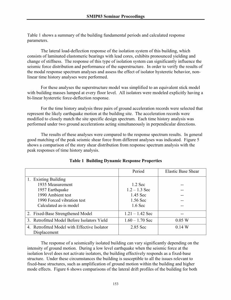
SMIP03 Seminar Proceedings
153
Table 1 shows a summary of the building fundamental periods and calculated response parameters.
The lateral load-deflection response of the isolation system of this building, which consists of laminated elastomeric bearings with lead cores, exhibits pronounced yielding and change of stiffness. The response of this type of isolation system can significantly influence the seismic force distribution and performance of the superstructure. In order to verify the results of the modal response spectrum analyses and assess the effect of isolator hysteretic behavior, non-linear time history analyses were performed.
For these analyses the superstructure model was simplified to an equivalent stick model with building masses lumped at every floor level. All isolators were modeled explicitly having a bi-linear hysteretic force-deflection response.
For the time history analysis three pairs of ground acceleration records were selected that represent the likely earthquake motion at the building site. The acceleration records were modified to closely match the site specific design spectrum. Each time history analysis was performed under two ground accelerations acting simultaneously in perpendicular directions.
The results of these analyses were compared to the response spectrum results. In general good matching of the peak seismic shear force from different analyses was indicated. Figure 5 shows a comparison of the story shear distribution from response spectrum analysis with the peak responses of time history analysis.
Table 1 Building Dynamic Response Properties Period Elastic Base Shear
1. Existing Building 1935 Measurement 1957 Earthquake 1990 Ambient test 1990 Forced vibration test Calculated as-is model
1.2 Sec
1.2 – 1.3 Sec 1.45 Sec 1.56 Sec 1.6 Sec
-- -- -- -- --
2. Fixed-Base Strengthened Model 1.21 – 1.42 Sec -- 3. Retrofitted Model Before Isolators Yield 1.60 – 1.70 Sec 0.05 W 4. Retrofitted Model with Effective Isolator
Displacement 2.85 Sec 0.14 W
The response of a seismically isolated building can vary significantly depending on the
intensity of ground motion. During a low level earthquake when the seismic force at the isolation level does not activate isolators, the building effectively responds as a fixed-base structure. Under these circumstances the building is susceptible to all the issues relevant to fixed-base structures, such as amplification of ground motion within the building and higher mode effects. Figure 6 shows comparisons of the lateral drift profiles of the building for both

SMIP03 Seminar Proceedings
154
design level and lower level earthquakes. The low level earthquake was arbitrarily defined as that having a base shear just below the trigger force of the isolators. Figure 6 indicates that, in this building, the low level earthquake can induce interstory drifts of the same order of magnitude as the design level event. This load condition was also considered for checking the critical building components.
Lateral Load Path of the Seismically Upgraded Building
The building has four distinct sections, each with its own lateral load resisting system: The clocktower, office tower, podium and basement. Refer to Figure 1. Clocktower
The clocktower, because of its slender configuration, and inherent overturning problems and damage-prone masonry infill, required a steel braced frame be added inside the clocktower. This braced frame was designed to resist the entire lateral load of the clocktower, not depending on the masonry infill to resist any of the lateral load. The stiffness of the new braced frame was selected to limit the clocktower structure ultimate inter-story drift to 0.008 times the story height to control potential damage to the infill brick/terra cotta cladding.
The base of this new steel braced frame “tower” is supported on a system of six interconnected steel transfer trusses that span 63 feet in the east-west direction and 62 feet in the north-south direction. The top chords of the one-story-deep trusses are located just below the 14th floor and the bottom chords are located just below the 13th floor. These trusses are supported on a system of eight new steel columns that extend down to the basement trusses by way of a new transfer truss system at the mezzanine level near the base of the office tower. The trusses and columns were designed to be stiff enough to limit drift in the clocktower due to overturning, i.e., the trusses “spread out” the reactions from the clocktower overturning moment.
Lateral loads from the base of the new clocktower braced frame are delivered to the exterior walls of the office tower portion of the building by a new horizontally braced diaphragm located just below the 14th floor. Office Tower
In order to assess the participation of the existing masonry materials in the resistance of future lateral loads, extensive in-situ testing was performed on the existing brick infill to determine its strength and stiffness properties (see “Assessment of Dynamic Response of Building” above). It was determined that 100% of the lateral forces could be resisted by the north-south (longitudinal) masonry infill walls in the 10-story office tower portion of the building. In the transverse direction, since the walls are shorter in length, it was determined that supplemental bracing was required in the east-west direction to control potential damage to these walls. Two lines (4 bays) of concentric steel braced frames, supported by the same eight new columns that support the clocktower trusses, were designed to resist approximately 25% of the lateral load in the transverse direction; the remaining 75% would be resisted by the existing infill frame walls. These braced frames extend down to the 7th floor where they transition to concrete

SMIP03 Seminar Proceedings
155
shear walls. The new braced frames were designed to be compatible with the stiffness of the existing transverse infill masonry walls. New steel collector beams were added at all floors to deliver lateral loads to the new braced frames and shear walls. Podium
In order to sufficiently stiffen the podium portion of the building to protect the historic hollow clay tile partitions and plaster, a system of new interior concrete shear walls, located in the core areas, was designed to extend down to the trusses in the basement. The locations of the faces of these new shear walls had to be carefully coordinated with the architectural historic finishes. Steel shear walls were used at some locations to reduce required shear wall proportions where existing exterior windows could not be closed off for historic reasons.
All of the new concrete shear walls are bounded by either new or existing steel columns. These columns are engaged by the new walls to act as boundary steel to resist wall overturning moments. Steel reinforcing plates (up to 4 inches thick) are added between the flanges of the existing columns as needed to provide sufficient boundary steel area. Basement
The concrete shear walls terminate on new 8.5 feet deep continuous steel “outrigger” trusses in the basement. Typically, double lines of trusses straddle and weld to the existing columns. These trusses are encased in concrete to provide additional stiffness and to tie the double lines of trusses together. The purpose of the trusses is to distribute the building overturning moments over a broad footprint so that the base isolators located beneath the office tower perimeter will not be overloaded nor subjected to any appreciable uplift.
A system of horizontal steel braces forms a “diaphragm” below the first floor to deliver lateral loads to a system of 113 elastomeric isolation bearings, approximately half of which have lead cores.
The existing basement concrete walls have concrete side beams added on both sides so that the wall, after being cut, will span rigidly between base isolators to support the massive stone-clad exterior podium walls.
The isolators are supported on a system of existing and new steel/concrete pedestals that are supported on the existing concrete mat foundation. Multiple isolators (up to 4 per group) are used to support individual columns with dead loads in excess of 3300 kips each.
A continuous seismic gap around the building was provided. The isolators are proportioned to move laterally more than 17 inches during an M7 event on the Hayward Fault. The prototype isolator units were tested to approximately 23 inches of displacement, which exceeds the 1991 UBC equivalent static formula requirement of 19 inches.

SMIP03 Seminar Proceedings
156
Resolution of Isolator Uplift due to MCE Forces
The maximum uplift displacements due to the critical cases of an MCE overturning moment were estimated using a step by step, iterative, static ETABS analysis based on the peak dynamic nonlinear time-history ANSR analysis results. The potential for local isolator uplift at the interior columns beneath the office tower perimeter was demonstrated. This problem was resolved by bounding the analytical results and uplift tests on the prototype isolators and their connections.
The critical cases of lateral seismic loads were derived from the ANSR nonlinear time-history analysis. Story forces from the ANSR analysis were applied statically to the ETABS model. Two isolator anchorage conditions were modeled in order to bound the analytical results of the uplift analysis:
• Case 1. Isolators allowed to uplift vertically when net uplift tension occurs. • Case 2. Isolators bolted top and bottom.
For Case 1, a process of iteration was used to identify the isolators that could go into net
tension under the MCE lateral loading. After each analysis step, any isolators showing a tensile load were softened to simulate a doweled bearing condition. The maximum net column uplift displacement using this approach was calculated to be 0.11 inches for the case of uncracked concrete encasement of the basement outrigger trusses, and 0.25 inches for the case of cracked encasement.
Case 2 analysis was intended to provide the maximum tensile force that could be generated if all bearings were bolted. The tensile vertical stiffness was assumed to be equal to the vertical compression stiffness. Results from tests done in Japan on small-scale laminated rubber isolators (Ishida et al. 1991) indicate that vertical stiffness decreases significantly after the bearings reach a tensile stress of about 250 psi and will continue to decrease until failure at roughly 850 psi, corresponding to an axial strain of about 300%. In order to obtain a safe, conservative upper limit on the uplift tension, the isolator forces were calculated using the initial vertical stiffness multiplied by the Case 1 “free” vertical displacement. All isolator anchorage components, including the anchor bolts, were designed to resist the tension forces thus calculated.
The analysis results indicated that the tendency toward isolator uplift would coincide with maximum isolator horizontal displacement. The prototype test program therefore incorporated a combination of ¼-inch vertical upward displacement with the maximum horizontal displacement. The rigidly bolted isolator specimens remained undamaged for the test case, which validated the final selection of conventionally bolted (non-doweled) connections.
Jacking and Re-Support of Existing Columns
Seismic isolation of an existing building such as Oakland City Hall typically involves the complicated task of shoring the existing columns so they may be cut free from the foundation

SMIP03 Seminar Proceedings
157
allowing installation of the new isolator bearings. Extensive sequencing notes were developed as part of the shoring design to guide the contractor during the bidding and construction phases.
The sequence notes were intended to help preserve the local and global structural integrity of the building to the extent practicable during construction. To achieve this goal, detail requirements for the following topics were included:
• Temporary lateral bracing was required for the basement level during the period of time between structural demolition and final release of the isolator system. Even partial demolition of the perimeter walls during isolator installation would cause a very weak story condition and put the building basement at risk of being damaged during a moderate or major earthquake if no temporary bracing was provided.
• A symmetric work sequence was required to reduce the possibility of an undesirable torsional response of the structure to an earthquake during the construction period.
• The magnitude of jacking loads and load application points were provided on the drawings. Typically, the jacking points were located on new steel framing and corbels welded to the existing columns. The new corbels also serve as permanent column bases after removal of the existing base plates.
• Vertical column displacement during jacking was limited in the contract documents to prevent damage to the superstructure finishes. This displacement was measured during jacking operations using sensitive instrumentation.
• Submittal and review of the contractors’ detailed construction sequence was required to ensure proper interpretation of the design intent.
Protection of Historically Sensitive Brittle Elements
The podium portion of the building (Floors 1, 2 and 3) contains the most prominent
public spaces and has the majority of the interior historic finishes. The unreinforced hollow clay tile (HCT) partition walls in the podium required special details to repair existing cracks caused by the Loma Prieta earthquake. Crack repair details were developed to allow the existing HCT to remain without replacing cracked tiles and to require only minimal removal of historic plaster finishes. This was accomplished using a combination of self-tapping anchors, metal lath, epoxy, and cement plaster.
Many of the exterior terra cotta cladding elements were also damaged during the earthquake. The damaged pieces were removed and used to create molds for the casting of new replacement pieces. New attachment details were developed to attach these replacement units.
Conclusions
The use of seismic base isolation as a seismic upgrade strategy dramatically reduced expected seismic force levels in the building and resulted in fewer shear walls than a traditional upgrade would have required. With fewer shear walls, the impact of the upgrade on the historically sensitive interior of this landmark building was significantly reduced. Base isolation proved to be an economically feasible solution when compared to conventional fixed base upgrade schemes. Through a combination of base isolation, extensive testing of the existing

SMIP03 Seminar Proceedings
158
masonry infill walls and a comprehensive finite element study of typical wall panels, the majority of seismic lateral forces will be resisted by existing unreinforced masonry infill walls in the office tower portion of the building.
By designing stiff concrete encased trusses in the basement, seismic overturning forces from this relatively tall building will be spread out over many base isolators so that they will not be overloaded nor subjected to appreciable uplift.
Acknowlegements Owner: City of Oakland Executive Architect: VBN Architects Structural Engineer: Forell/Elsesser Engineers, Inc. (Base Isolation and Building Repairs and Retrofit) Messinger & Associates (Post-Earthquake Studies) Consultants to F/E: Messinger & Associates Razzano Associates Tennebaum-Manheim Engineers Geotechnical: Dames & Moore Peer Review: Wiss, Janney, Elstner Associates
References Benjamin, J.R. and Williams, H.A., “The Behavior of One-Story Brick Shear Walls,” ASCE Proceedings, Volume 84, No St. 4, July 1958, p. 1723. Earthquake Investigations in California, Special Publication No. 201, U.S. Department of Commerce, U.S. Government Printing Office, Washington, 1936, p.55. Recommended Lateral Force Requirements and Commentary (“Bluebook”), 1990 Edition by Seismology Committee of Structural Engineers Association of California. Uniform Building Code, International Conference of Building Officials, Whittier, CA, 1991. VBN Architects and Michael Willis and Associates, “Evaluation of Earthquake Damage and Repair Required by Code,” Final Report in 5 Volumes for the City of Oakland, November 1990. Zaric, R. “Masonry-Infilled Reinforced Concrete Frames on Subassemblies of Earthquake-Resistant Buildings,” Earthquake Damage Evaluation and Vulnerability Analysis of Building Structures, Karidze, A. Editor, UNESCO, Omega Eng. Oxford, England, p. 79-100.
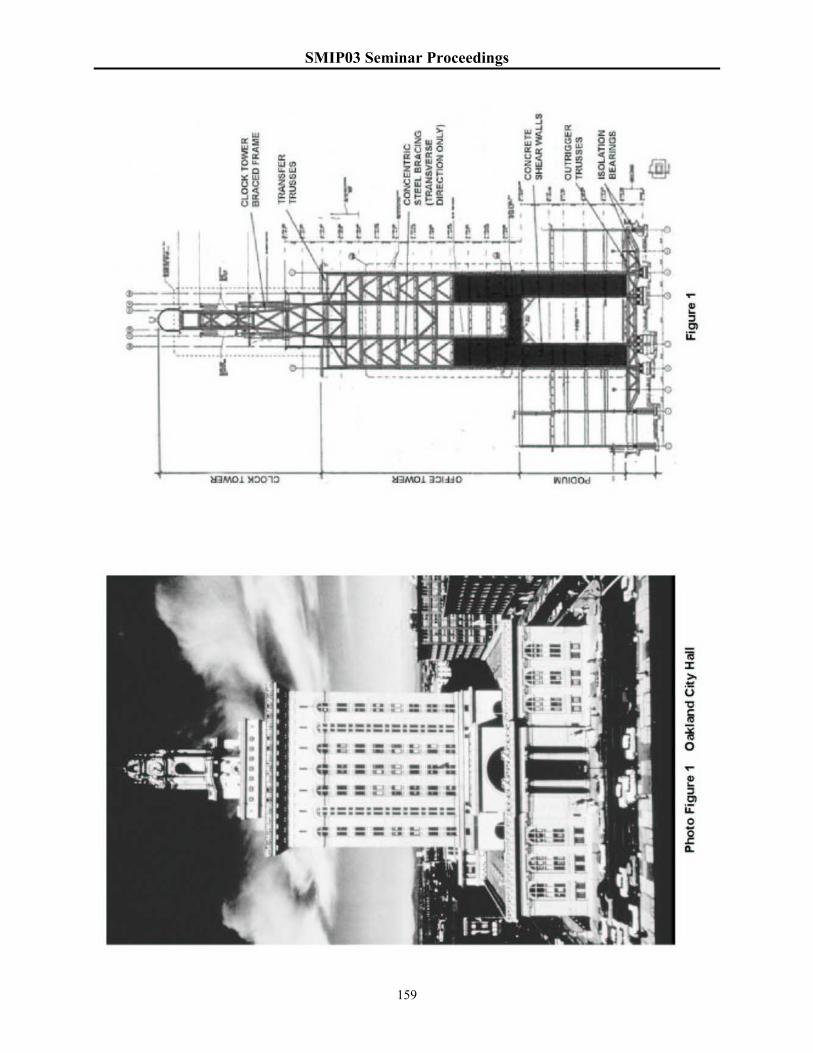
SMIP03 Seminar Proceedings
159

SMIP03 Seminar Proceedings
160
Figure 4
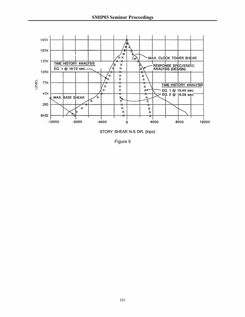
SMIP03 Seminar Proceedings
161
Figure 5

SMIP03 Seminar Proceedings
162
Figure 6
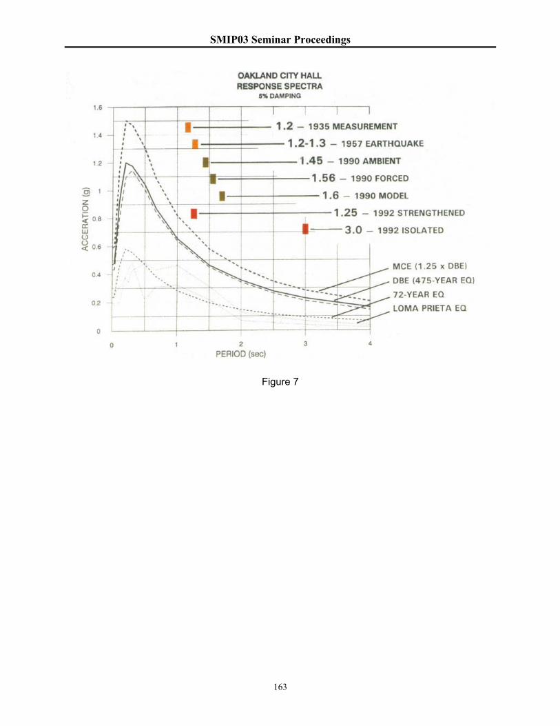
SMIP03 Seminar Proceedings
163
Figure 7

SMIP03 Seminar Proceedings
164

SMIP03 Seminar Proceedings
165
STRONG-MOTION INSTRUMENTATION OF THE OAKLAND CITY HALL
Moh Huang, Anthony Shakal and Carl Petersen
Strong Motion Instrumentation Program California Geological Survey Department of Conservation
Sacramento, California
Abstract The Oakland City Hall was strengthened after the 1989 Loma Prieta earthquake and instrumented with 21 sensors by the California Strong Motion Instrumentation Program in 1995. This paper describes the sensor locations in the City Hall and the instrumentation objectives. Low amplitude strong-motion records that were obtained from the instrumentation at the City Hall during the magnitude 4.9 Gilroy earthquake of May 13, 2002 are also presented and discussed.
Introduction The Oakland City Hall, constructed in 1914, is a historic landmark. It is an eighteen-story building, crowned with a decorative three-story clock tower. It was designed in 1911. In elevation the building can be divided into three sections: the podium, the office tower, and the clock tower (Figures 1 and 2). The podium is 124′ by 179′ in plan and rises to a height of 70′ above the ground. On top of the podium is a twelve-story office tower (66′ by 102′ in plan) that rises to a height of 206′. The building steps back once more above this level (14th Floor) and rises to the 16th Floor at a height of 232′. The 18th Floor is the base of the clock that rises to a final height of 305′. The building has a complete basement floor 14′ in height. The load bearing system in the building consists of riveted steel frames made up of rolled shapes and built-up sections of angles and plates. For the purpose of fire-proofing, steel elements are enclosed in brick masonry, unreinforced concrete or hollow clay tiles (HCT). The exterior walls are the major lateral load resisting elements in the podium and the office tower. They are composed of infill unreinforced brick masonry faced with granite and terra cotta ornamentation. The interior partitions are hollow clay tiles, and the ceilings and walls are finished with plaster. A typical floor in the building consists of a 5″ thick reinforced concrete slab supported on steel frames. The shear forces at the base of the office tower are transferred through the podium roof diaphragm to the exterior walls of the podium. The overturning moments at the base of the office

SMIP03 Seminar Proceedings
166
Figure 1. View of the Oakland City Hall from the Plaza.
Figure 2. View of the Oakland City Hall from the roof of an adjacent high-rise building.
SMIP03 Seminar Proceedings
167
tower are carried by axial forces in the columns aligned with the exterior walls of the office tower. These columns are continuous from the office tower through the podium and to the foundation. The building foundation consists of a 2′4″ deep concrete mat over the entire basement area. Building columns are supported on a framework of structural steel beams embedded within the concrete mat. The soil at the building site consists of sand and clay that becomes very dense and stiff below 100′. The bedrock is estimated at a depth of 400′ to 500′ (Dames & Moore, 1990).
Seismic Strengthening During the 1989 Loma Prieta Earthquake, the clock tower and its supporting steel frame were severely damaged (Button, et al., 1991). The northern URM wall of the clock tower shifted almost one inch off its base at the 16th floor level. The floor beams supporting the clock tower had diagonal shear fractures through the web. These cracks were caused by the overturning forces of the clock tower. Cracking also occurred in the perimeter walls at the 16th floor. The terra-cotta ornamentation at the 16th floor showed evidence of spalling. The main steel frame in the podium and the office tower was not damaged. Many interior hollow clay tile partitions in the office tower and the podium suffered extensive cracking.
In strengthening the City Hall, 111 lead-rubber seismic isolation bearings were used to isolate the building at the top of the existing mat foundation (Honeck, et al., 1994; Walters, 2003). Simultaneously, new concrete shear walls and braced steel frames were added to strengthen and stiffen the existing lateral load resisting system for the superstructure (Figure 3). A system of 6′6″ deep steel outrigger trusses encased with concrete was added at the basement level to spread out the seismic overturning forces to isolator bearings mounted on concrete pedestals rising from the mat foundation. The trusses will limit the uplift at the isolators to 0.25 inch (Honeck and Walters, 1994). The isolators were designed to undergo a maximum horizontal displacement of approximately 11 inches. In the podium and tower structure new concrete shear walls and steel braces were added. In the transverse direction, concrete shear walls were added up to the 7th floor level and concentric braced steel frames were added from the 7th to the 14th floors. These braced frames were designed to share loads with existing URM perimeter walls (Elsesser, 1993; Walters, 2003). In the longitudinal direction concrete shear walls were added up to the 4th floor level only. No braced frames were added in this direction. The clock tower was strengthened by adding a steel 3-D space frame in its interior that rises from the 14th floor level. The original base of the clock tower was at the 16th floor level. At the 14th floor level, loads from the clock tower are transmitted to the exterior and interior columns below by new transfer trusses. The top chord of transfer trusses is just below the 14th floor level and the bottom chord is just below the 13th floor level. The new seismic force resisting system, together with the existing structure, was designed to resist a base shear of 13% of the weight of the structure, as transmitted by the base isolators. The seismic repair design was in accordance with the 1991 City of Oakland Building Code (equivalent to 1988 UBC). The design of the base isolation system was in accordance with

SMIP03 Seminar Proceedings
168
the appendix to Chapter 23 of the 1991 Uniform Building Code. The design was also based on the site-specific response spectra with 475-year return period (Dames and Moore, 1990). Dynamic response analyses of the structure using ETABS and ANSR programs were performed (Honeck and Walters, 1994). The input motions for the computer models were the strong-motion records from the Loma Prieta earthquake obtained by CSMIP at a nearby 2-story building and the artificial acceleration time histories generated from the design earthquake.
Strong-Motion Instrumentation and Records Records from the 1957 San Francisco Earthquake The Oakland City Hall was originally instrumented prior to the San Francisco earthquake of March 22, 1957. The accelerographs were installed at the basement and on the 16th floor. The recorded peak horizontal accelerations were 9.0% g on the 16th floor and 4.0% g at the basement from the main shock of the 1957 San Francisco earthquake (magnitude 5.3, distance 24 km). A magnitude 4.4 aftershock was also recorded at the City Hall (Caltech EERL, 1976) During the 1957 San Francisco earthquake the structure exhibited a fundamental vibration period of 1.2 to 1.3 seconds. From the forced vibration tests conducted after the Loma Prieta earthquake the fundamental periods were determined to be 1.56 seconds (E-W), 1.32 seconds (N-S) and 0.74 seconds (Torsional) (ANCO, 1990). The period of the original structure was modeled by the computer at 1.6 seconds. According to the soil-structure interaction analysis by Dames and Moore (1990), the soil-structure interaction has essentially no effect on the fundamental period of the building. The fixed-base period of the structure was lowered to 1.25 seconds by addition of concrete shear walls and steel braces (Elsesser, 1993; Walters, 2003). The base-isolated structure has a period of 2.8 seconds. In summary, the building fundamental periods are: 1935 vibration tests 1.2 seconds 1957 earthquake 1.2-1.3 seconds 1990 ambient 1.45 seconds 1990 forced vibration 1.56 sec. (E-W), 1.32 sec. (N-S) As-is model 1.6 seconds Strengthened (fixed base) 1.25 seconds Strengthened (base-isolated) 2.8 seconds Strong-Motion Instrumentation in 1995 The planning for the instrumentation of the Oakland City Hall began in early 1992. The instrumentation was completed in June 1995 at the last stage of the seismic strengthening work. In general, instrumentation of a building involves the installation of accelerometers or other sensors at key locations throughout the structure. The number and location of sensors determines the amount of information that may be recovered about the response of the building after an earthquake. Sensors installed at key structural members allow the important modes of vibration to be recorded and specific measurement objectives to be achieved. Optimal locations
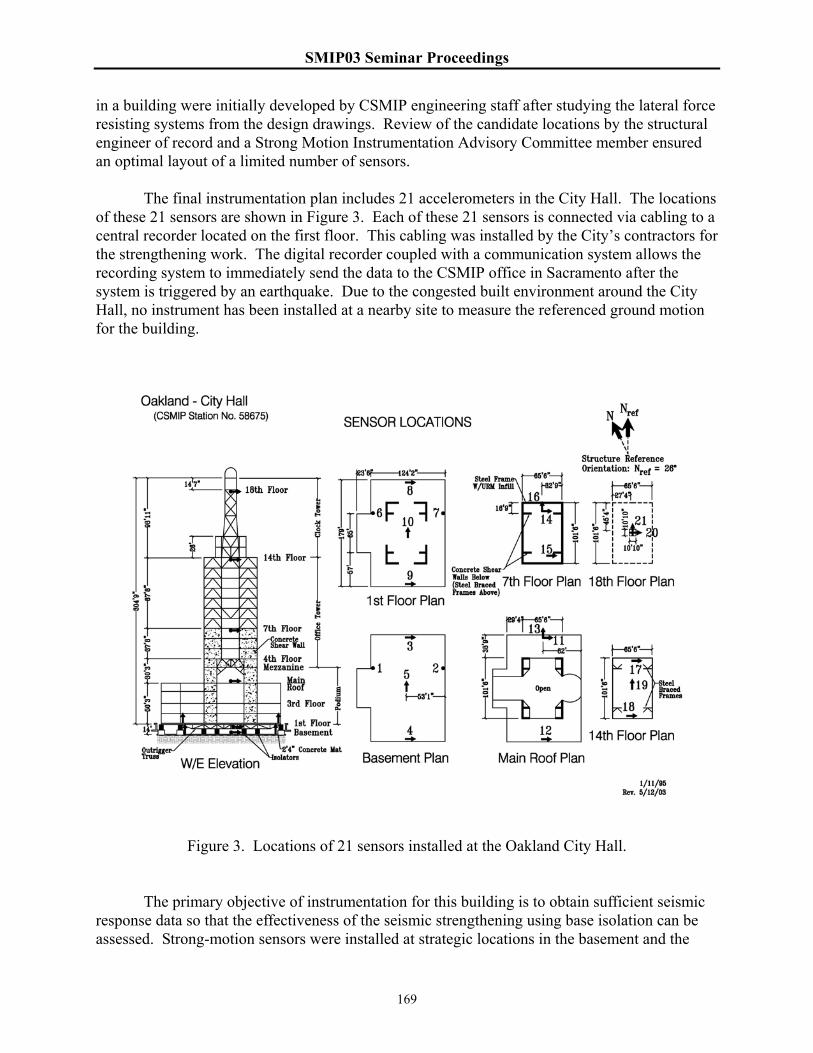
SMIP03 Seminar Proceedings
169
in a building were initially developed by CSMIP engineering staff after studying the lateral force resisting systems from the design drawings. Review of the candidate locations by the structural engineer of record and a Strong Motion Instrumentation Advisory Committee member ensured an optimal layout of a limited number of sensors. The final instrumentation plan includes 21 accelerometers in the City Hall. The locations of these 21 sensors are shown in Figure 3. Each of these 21 sensors is connected via cabling to a central recorder located on the first floor. This cabling was installed by the City’s contractors for the strengthening work. The digital recorder coupled with a communication system allows the recording system to immediately send the data to the CSMIP office in Sacramento after the system is triggered by an earthquake. Due to the congested built environment around the City Hall, no instrument has been installed at a nearby site to measure the referenced ground motion for the building.
Figure 3. Locations of 21 sensors installed at the Oakland City Hall.
The primary objective of instrumentation for this building is to obtain sufficient seismic response data so that the effectiveness of the seismic strengthening using base isolation can be assessed. Strong-motion sensors were installed at strategic locations in the basement and the
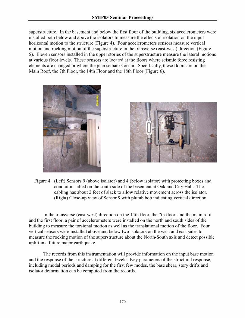
SMIP03 Seminar Proceedings
170
superstructure. In the basement and below the first floor of the building, six accelerometers were installed both below and above the isolators to measure the effects of isolation on the input horizontal motion to the structure (Figure 4). Four accelerometers sensors measure vertical motion and rocking motion of the superstructure in the transverse (east-west) direction (Figure 5). Eleven sensors installed in the upper stories of the superstructure measure the lateral motions at various floor levels. These sensors are located at the floors where seismic force resisting elements are changed or where the plan setbacks occur. Specifically, these floors are on the Main Roof, the 7th Floor, the 14th Floor and the 18th Floor (Figure 6).
Figure 4. (Left) Sensors 9 (above isolator) and 4 (below isolator) with protecting boxes and
conduit installed on the south side of the basement at Oakland City Hall. The cabling has about 2 feet of slack to allow relative movement across the isolator. (Right) Close-up view of Sensor 9 with plumb bob indicating vertical direction.
In the transverse (east-west) direction on the 14th floor, the 7th floor, and the main roof and the first floor, a pair of accelerometers were installed on the north and south sides of the building to measure the torsional motion as well as the translational motion of the floor. Four vertical sensors were installed above and below two isolators on the west and east sides to measure the rocking motion of the superstructure about the North-South axis and detect possible uplift in a future major earthquake. The records from this instrumentation will provide information on the input base motion and the response of the structure at different levels. Key parameters of the structural response, including modal periods and damping for the first few modes, the base shear, story drifts and isolator deformation can be computed from the records.
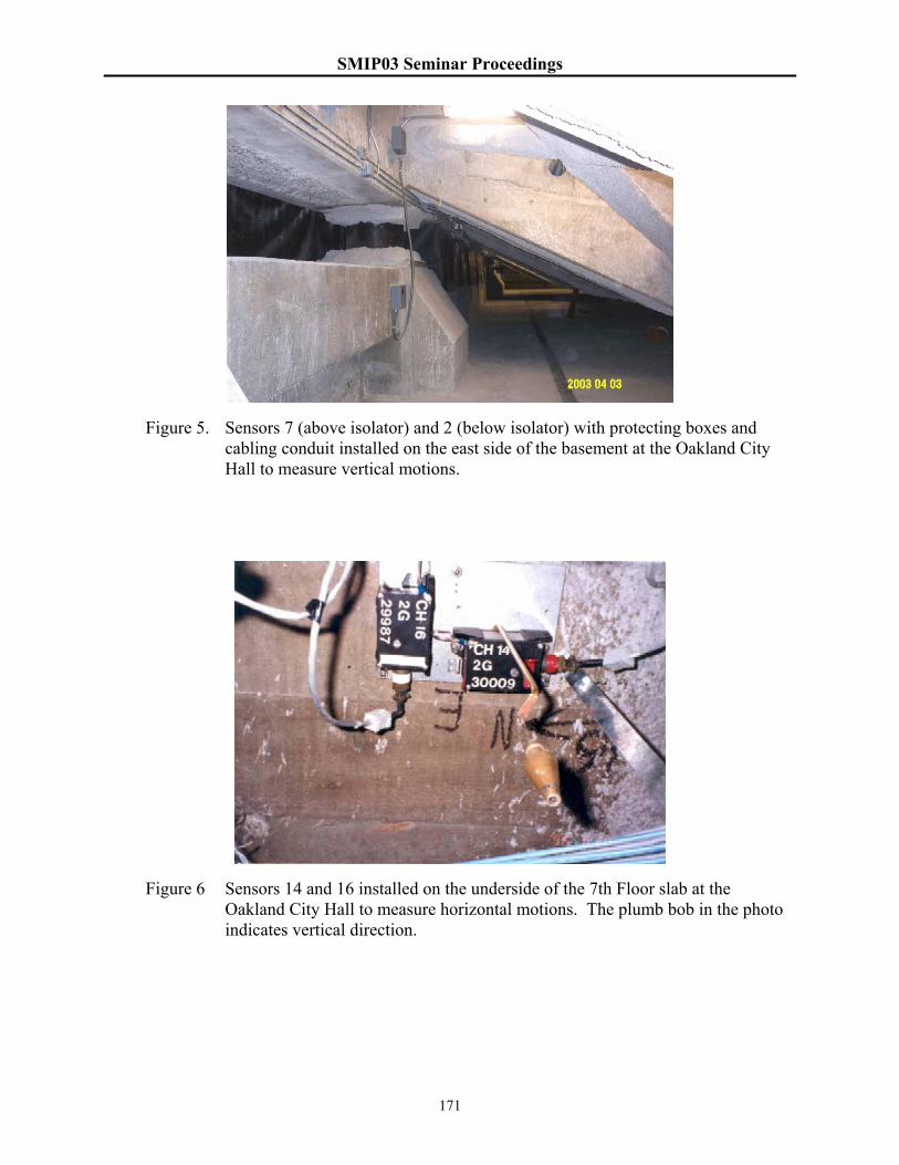
SMIP03 Seminar Proceedings
171
Figure 5. Sensors 7 (above isolator) and 2 (below isolator) with protecting boxes and cabling conduit installed on the east side of the basement at the Oakland City Hall to measure vertical motions.
Figure 6 Sensors 14 and 16 installed on the underside of the 7th Floor slab at the Oakland City Hall to measure horizontal motions. The plumb bob in the photo indicates vertical direction.
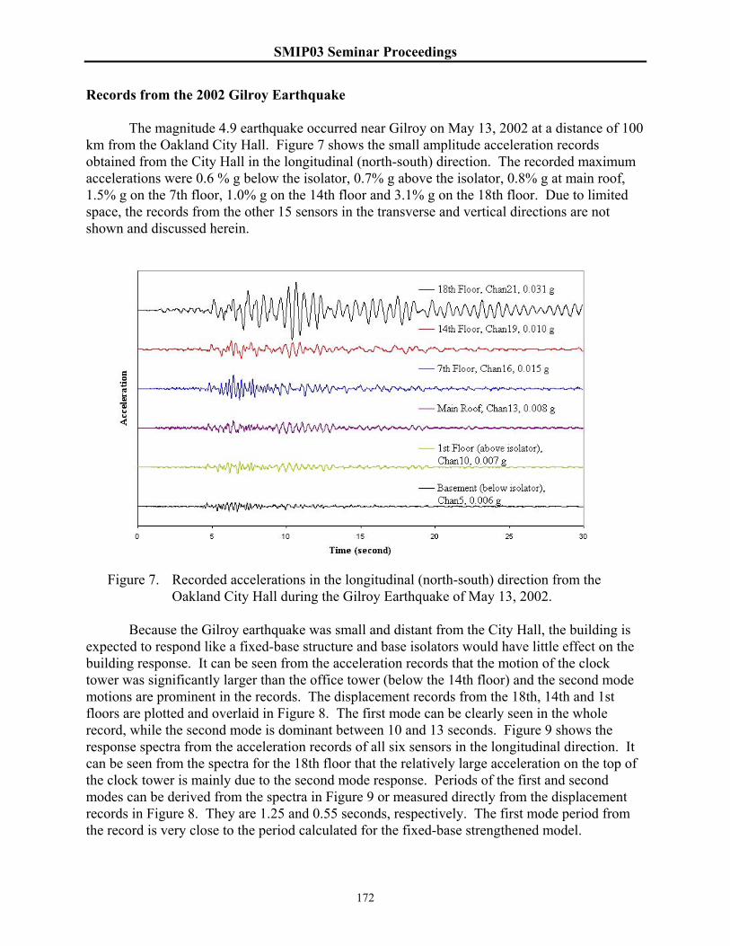
SMIP03 Seminar Proceedings
172
Records from the 2002 Gilroy Earthquake The magnitude 4.9 earthquake occurred near Gilroy on May 13, 2002 at a distance of 100 km from the Oakland City Hall. Figure 7 shows the small amplitude acceleration records obtained from the City Hall in the longitudinal (north-south) direction. The recorded maximum accelerations were 0.6 % g below the isolator, 0.7% g above the isolator, 0.8% g at main roof, 1.5% g on the 7th floor, 1.0% g on the 14th floor and 3.1% g on the 18th floor. Due to limited space, the records from the other 15 sensors in the transverse and vertical directions are not shown and discussed herein.
Figure 7. Recorded accelerations in the longitudinal (north-south) direction from the
Oakland City Hall during the Gilroy Earthquake of May 13, 2002. Because the Gilroy earthquake was small and distant from the City Hall, the building is expected to respond like a fixed-base structure and base isolators would have little effect on the building response. It can be seen from the acceleration records that the motion of the clock tower was significantly larger than the office tower (below the 14th floor) and the second mode motions are prominent in the records. The displacement records from the 18th, 14th and 1st floors are plotted and overlaid in Figure 8. The first mode can be clearly seen in the whole record, while the second mode is dominant between 10 and 13 seconds. Figure 9 shows the response spectra from the acceleration records of all six sensors in the longitudinal direction. It can be seen from the spectra for the 18th floor that the relatively large acceleration on the top of the clock tower is mainly due to the second mode response. Periods of the first and second modes can be derived from the spectra in Figure 9 or measured directly from the displacement records in Figure 8. They are 1.25 and 0.55 seconds, respectively. The first mode period from the record is very close to the period calculated for the fixed-base strengthened model.

SMIP03 Seminar Proceedings
173
Figure 8. Displacements at the 18th Floor, the 14th Floor and the 1st Floor in the
longitudinal (north-south) direction from the Oakland City Hall during the Gilroy Earthquake of May 13, 2002.
Figure 9. Acceleration response spectra (2% damping) of the records in the longitudinal
(north-south) direction from the Oakland City Hall during the Gilroy Earthquake of May 13, 2002.

SMIP03 Seminar Proceedings
174
The displacement records from sensors above and below the isolator are plotted and compared in Figure 10. The deformation of the isolator can be calculated by differencing these two displacement records. The isolator deformation is smaller than 0.01 cm and much less than the design displacement of 28 cm or 11 inches.
Figure 10. Displacements above and below the isolator in the longitudinal (north-south)
direction from the Oakland City Hall during the Gilroy Earthquake of May 13, 2002.
Summary The California Strong Motion Instrumentation Program installed strong-motion equipment at the Oakland City Hall during the seismic strengthening project in 1995 with assistance and cooperation from the City of Oakland. The instrumentation system will record building response data from which effectiveness of the seismic strengthening using base isolation, as well as the seismic safety, can be assessed after future significant earthquakes. The recorded data will be available so the near-real-time data can be used for post-earthquake evaluation of the building performance.
Acknowledgement The California Strong Motion Instrumentation Program extends its appreciation to staff of the City of Oakland who has permitted and cooperated in the installation and maintenance of strong-motion equipment in the City Hall. The City staff includes Ezra Rapport, Veronica

SMIP03 Seminar Proceedings
175
Martin, Caroline Soohool, and William Weber. CSMIP also extends its appreciation to members of the Strong Motion Instrumentation Advisory Committee and its Buildings Subcommittee in recommending the City Hall for instrumentation. Mason Walters of Forell/Elsesser Engineers and Anna Dal Pino of Degenkolb Engineers reviewed and commented on the proposed sensor locations. The instrumentation of the Oakland City Hall was made possible through the efforts of CSMIP engineers and technicians who planned and installed the instrumentation. Praveen Maholtra was the project engineer. The instrumentation was installed by Steve Fife, Tom Pierce and Neil Adler. References ANCO (1990). "Forced Vibration Testing of the Oakland City Hall," Report Submitted to City of Oakland, Office of Public Works, April 1990. Button, M., Blondet, M., Mayes, R., Messinger, D., Quinn, J., Tovani, R., Elsesser, E. and Walters, M., (1991). "Oakland City Hall: Performance Analysis and Seismic Isolation Retrofit," Proceedings of the 60th Annual Convention, Structural Engineers Association of California, Palm Springs, October 1991. Caltech EERL (1976). "Strong Motion Earthquake Acclerograms Index Volume," Report No. EERL 76-02, Caltech Earthquake Engineering Research Laboratory, August 1976. Dames & Moore (1990). "Site Specific Seismic Hazard Analysis," Report Submitted to City of Oakland, August 10, 1990. Elsesser, E. , (1993). "The Seismic Repair and Rehabilitation of Oakland City Hall," EERI Technical Seminar on Seismic Rehabilitation of Existing Buildings, San Francisco and Los Angeles, January 1993. Honeck, W. and Walters, M., (1994). "Use of Steel in the Seismic Retrofit of Historic Oakland City Hall," Steel Tips by the Structural Steel Education Council, December 1994. Honeck, W.. Walters, M., Sattary, V. and Rodler, P., (1994). "Design and Implementation of Base Isolation for the Seismic Repair and Retrofit of Oakland City Hall,” Proceedings of the Fifth U.S. National Conference on Earthquake Engineering, Volume 1, Earthquake Engineering Research Institute, July 1994. Walters, M., (2003). "The Seismic Retrofit of the Oakland City Hall," SMIP03 Seminar Proceedings, Oakland, May 22, 2003.