smooth nonparametric bernstein vine copulas
TRANSCRIPT

arX
iv:1
210.
2043
v1 [
q-fin
.RM
] 7
Oct
201
2
Smooth Nonparametric Bernstein Vine Copulas
Gregor N.F. Weiß∗
Juniorprofessur fur Finance, Technische Universitat Dortmund
Marcus Scheffer†
Lehrstuhl fur Investition und Finanzierung, Technische Universitat Dortmund
October 27, 2021
Abstract We propose to use nonparametric Bernstein copulas as bivariate pair-copulas in high-
dimensional vine models. The resulting smooth and nonparametric vine copulas completely obvi-
ate the error-prone need for choosing the pair-copulas fromparametric copula families. By means
of a simulation study and an empirical analysis of financial market data, we show that our pro-
posed smooth nonparametric vine copula model is superior tocompeting parametric vine models
calibrated via Akaike’s Information Criterion.
Keywords: Risk management; Dependence structures; Vine Copulas; Bernstein Copulas.
JEL Classification Numbers: C52, C53, C58.
∗Address: Corresponding author; Otto-Hahn-Str. 6a, D-44227 Dortmund, Germany, telephone: +49 231 755 4608,e-mail:[email protected]
†Address: Otto-Hahn-Str. 6a, D-44221 Dortmund, Germany, telephone: +49 231 755 4231, e-mail:[email protected]. We are grateful to Janet Gabrysch, Sandra Gabrysch, DanielHustert, Felix Ir-resberger and Janina Muhlnickel for their outstanding research assistance. Support by the Collaborative ResearchCenter ”Statistical Modeling of Nonlinear Dynamic Processes” (SFB 823) of the German Research Foundation (DFG)is gratefully acknowledged.

1 Introduction
Following the growing criticism of elliptical models, copulas have emerged both in insurance
and risk management as a powerful alternative for modeling the complete dependence structure
of a multivariate distribution. Since the seminal work by Embrechts et al. (2002), the literature on
copulas and their use in risk management applications has grown exponentially with several studies
concentrating on statistical inference and model selection for copulas (see, e.g., Kim et al., 2007;
Genest et al., 2009b) as well as applications (see, e.g., Chan and Kroese, 2012; Grundke and Polle,
2012; Yea et al., 2012).1
As simple parametric models are often not flexible enough to model high-dimensional distri-
butions, recent works by Joe (1996, 1997), Bedford and Cooke(2001, 2002) and Whelan (2004)
have proposed copula models which are highly flexible but at the same time still tractable even
in higher dimensions. Most notably, vine copulas (also called pair-copula constructions, PCC in
short) have emerged as the most promising tool for modeling dependence structures in high dimen-
sions.2 Vine copulas consist of a cascade of conditional bivariate copulas (so called pair-copulas)
which can each be chosen from a different parametric copula family. As a result, vine copulas
are extremely flexible yet still tractable even in high dimensions as all computations necessary in
statistical inference are performed on bivariate data sets(see Aas et al., 2009, for a first discussion
of vine copulas in an applied setting).
Similar to the bivariate case,3 the correct selection of the parametric constituents of thevine,
i.e., the pair-copulas, is crucial for the correct specification of a vine copula model. In case of
the popular C- and D-vine specifications, the calibration and estimation of ad-dimensional vine
requires the selection and estimation ofd(d− 1)/2 different pair-copulas from the set of candidate
bivariate parametric copula families. Thus, a vine model’sincreased flexibility only comes at the
expense of an increased model risk.
As a remedy, recent studies have suggested to select the parametric pair-copulas based on
graphical data inspection and goodness-of-fit tests (Aas etal., 2009) and to employ sequential
heuristics based on Akaike’s Information Criterion (AIC) (see, e.g., Brechmann et al., 2012;
Dißmann et al., forthcoming). Kurowicka (2010) and Brechmann et al. (2012) propose strate-
gies for simplifying vines by replacing certain pair-copulas by the independence copula (yield-
ing a truncated vine copula) or the Gaussian copula (yielding asimplified vine). Finally,
1A literature review with a special emphasis on finance-related papers using copulas is given by Genest et al.(2009a). An overview of the different branches of the copulaliterature is given by Embrechts (2009).
2Competing modeling concepts like nested and hierarchical Archimedean copulas are analyzed by Aas and Berg(2009) as well as Fischer et al. (2009). They conjecture thatvine copulas should be preferred over nested or hierarchi-cal Archimedean copulas.
3See Genest et al. (2009b), Kole et al. (2007) and Weiß (2011, 2012) for discussions of the problem of selectingthe best fitting parametric copula.
1
Hobæk-Haff and Segers (2012) propose the use of empirical pair-copulas in vine models to cir-
cumvent the problem of selecting parametric pair-copulas.
In this paper, we use the recently proposed nonparametric Bernstein copulas
(Sancetta and Satchell, 2004; Pfeifer et al., 2009; Diers etal., 2012) as pair-copulas yielding
smooth nonparametric vine copula models that do not requirethe specification of parametric
families. Thus, we extend the ideas laid out by Hobæk-Haff and Segers (2012) by using an ap-
proximation to the empirical pair-copulas. In contrast to their work, however, we approximate the
pair-copulas not only nonparametrically but also by the useof continuous functions.4 In addition,
especially the Bernstein copula has recently attracted attention in insurance modeling (Diers et al.,
2012) and has already proven its merits in an applied setting. Therefore, the contributions of the
proposed smooth nonparametric vine copulas are twofold: First, the use of Bernstein copulas
completely obviates the need for the error-prone selectionof pair-copulas from pre-specified
sets of parametric copulas. The resulting smooth and nonparametric vine copulas do not only
constitute extremely flexible tools for modeling high-dimensional dependence structures, they are
also characterized by a smaller model risk than their parametric counterparts. Second, Bernstein
copulas have been shown to improve on the estimation of the underlying dependence structure by
competing nonparametric empirical copulas.5 The modeling of a vine model’s pair-copulas by the
use of smooth approximating functions is thus a natural extension of recently proposed (highly
discontinuous) empirical pair-copulas.
The usefulness of the proposed Bernstein vines is demonstrated by means of a simulation
study as well as by forecasting and backtesting the Value-at-Risk (VaR) for multivariate portfolios
of financial assets.
The results presented in this study show that our proposed vine copula model with smooth non-
parametric Bernstein pair-copulas outperforms the benchmark model with parametric pair-copulas
in higher dimensions with respect to the accuracy and numerical stability of the approximation
to the true underlying dependence structure. While our nonparametric vine copula model yields
worse average squared errors than a benchmark vine copula calibrated by selecting parametric
pair-copulas based on AIC values in lower dimensions (e.g.,d = 3, 5, 7) in our simulations, this
result is reversed in higher dimensions. For random vectorsof dimensiond = 11 and higher, the
parametric benchmark broke down in more than50% of the simulations due to either the numerical
4Using smooth functions to approximate the true underlying dependence structure is in line with our intuition.The superiority of smooth nonparametric approximations ofthe copula over simple empirical copulas, however, isalso found by Shen et al. (2008). They argue that the improvedapproximation by the linear B-spline copulas is due totheir Lipschitz continuity.
5For example, Bernstein copulas provide a higher rate of consistency than other common nonparametric estimatorsand do not suffer from boundary bias (Kulpa, 1999; Sancetta and Satchell, 2004; Diers et al., 2012). Similarly, otherapproximations as, e.g., linear B-spline copulas have alsobeen shown to yield lower average squared approximationerrors than competing discrete approximations (Shen et al., 2008).
2

instability of the parameter and AIC estimation or simply due to extremely inaccurate approxima-
tions caused by badly selected parametric pair-copulas. Inhigher dimensions (i.e., the main field
of application of vine copulas), our nonparametric modeling approach is thus clearly superior to
a parametric vine copula model. Our risk management application, however, shows that even in
lower dimensions (d = 5) our nonparametric model yields VaR forecasts that are not rejected
by a range of formal statistical backtests. Consequently, the slightly worse approximation errors
of our nonparametric model in lower dimensions do not seem toaffect the modeling of a given
dependence structure too severely thus underlining the usefulness of our proposed model.
The remainder of this article is structured as follows. Section 2 introduces vine copulas as well
as Bernstein copulas which we employ as pair-copulas in the vines. Section 3 presents the results
of a simulation study on the approximation errors of both ournonparametric Bernstein vine copula
model as well as a heuristically calibrated parametric benchmark model. In Section 4, we conduct
an empirical analysis for a five-dimensional financial portfolio. Concluding remarks are given in
Section 5.
2 Smooth nonparametric vine copulas
The purpose of this section is to shortly introduce the fundamentals of vine and Bernstein
copulas.
2.1 Vine copulas
Vine copulas are obtained by hierarchical cascades of conditional bivariate copulas and are
characterized by an increased flexibility for modeling inhomogeneous dependence structures in
high dimensions. Here, we only present the basic definition as well as some basic properties of
two popular classes of vines, i.e., C- and D-vines,6 which will be used later on in our application to
financial market data. Readers interested in a more rigorousexamination of vine copulas and their
properties are referred to the excellent studies by Joe (1996, 1997) and Bedford and Cooke (2001,
2002).
Starting point is the well-known observation that a joint probability density function of dimen-
siond can be decomposed into
f(x1, . . . , xd) = f(x1) · f(x2|x1) · f(x3|x1, x2) · . . . · f(xd|x1, . . . , xd−1). (1)
6The classes of C- and D-vines are subsets of the so-called regular vines (or R-vines in short, see Brechmann et al.,2012). We do not consider other types of R-vines in this paperbut note that our proposed use of smooth Bernstein andB-spline copulas as pair-copulas can also be extended to other subsets of R-vines.
3
Each factor in this product can then be decomposed further using a conditional copula, e.g.
f(x2|x1) = c12(F1(x1), F2(x2)) · f2(x2) (2)
with Fi(·) being the cumulative distribution function (cdf) ofxi (i = 1, . . . , d) andc12(·) being the
(in this case unconditional) copula density of(x1, x2).
Going further down the initial decomposition, the conditional densityf(x3|x1, x2) could be
factorised via
f(x3|x1, x2) = c23|1(F2|1(x2|x1), F3|1(x3|x1)) · c13(F1(x1), F3(x3)) · f3(x3) (3)
with c23|1(·) being the conditional copula of(x2, x3) givenx1.
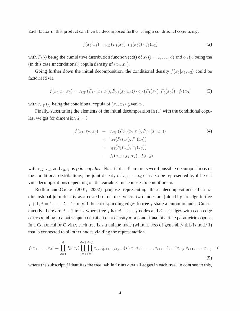
Finally, substituting the elements of the initial decomposition in (1) with the conditional copu-
las, we get for dimensiond = 3
f(x1, x2, x3) = c23|1(F2|1(x2|x1), F3|1(x3|x1)) (4)
· c12(F1(x1), F2(x2))
· c13(F1(x1), F3(x3))
· f1(x1) · f2(x2) · f3(x3)
with c12, c13 andc23|1 aspair-copulas. Note that as there are several possible decompositions of
the conditional distributions, the joint density ofx1, . . . , xd can also be represented by different
vine decompositions depending on the variables one choosesto condition on.
Bedford and Cooke (2001, 2002) propose representing these decompositions of ad-
dimensional joint density as a nested set of trees where two nodes are joined by an edge in tree
j + 1, j = 1, . . . , d − 1, only if the corresponding edges in treej share a common node. Conse-
quently, there ared − 1 trees, where treej hasd + 1 − j nodes andd − j edges with each edge
corresponding to a pair-copula density, i.e., a density of aconditional bivariate parametric copula.
In a Canonical or C-vine, each tree has a unique node (withoutloss of generality this is node1)
that is connected to all other nodes yielding the representation
f(x1, . . . , xd) =d∏
k=1
fk(xk)d−1∏
j=1
d−j∏
i=1
ci,i+j|i+1,...,i+j−1(F (xi|xi+1, . . . , xi+j−1), F (xi+j|xi+1, . . . , xi+j−1))
(5)
where the subscriptj identifies the tree, whilei runs over all edges in each tree. In contrast to this,
4
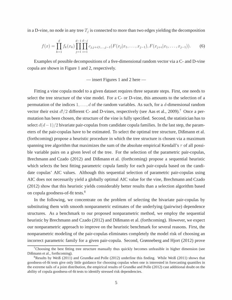
in a D-vine, no node in any treeTj is connected to more than two edges yielding the decomposition
f(x) =d∏
k=1
fk(xk)d−1∏
j=1
d−j∏
i=1
cj,j+i|1,...,j−1(F (xj|x1, . . . , xj−1), F (xj+i|x1, . . . , xj−1)). (6)
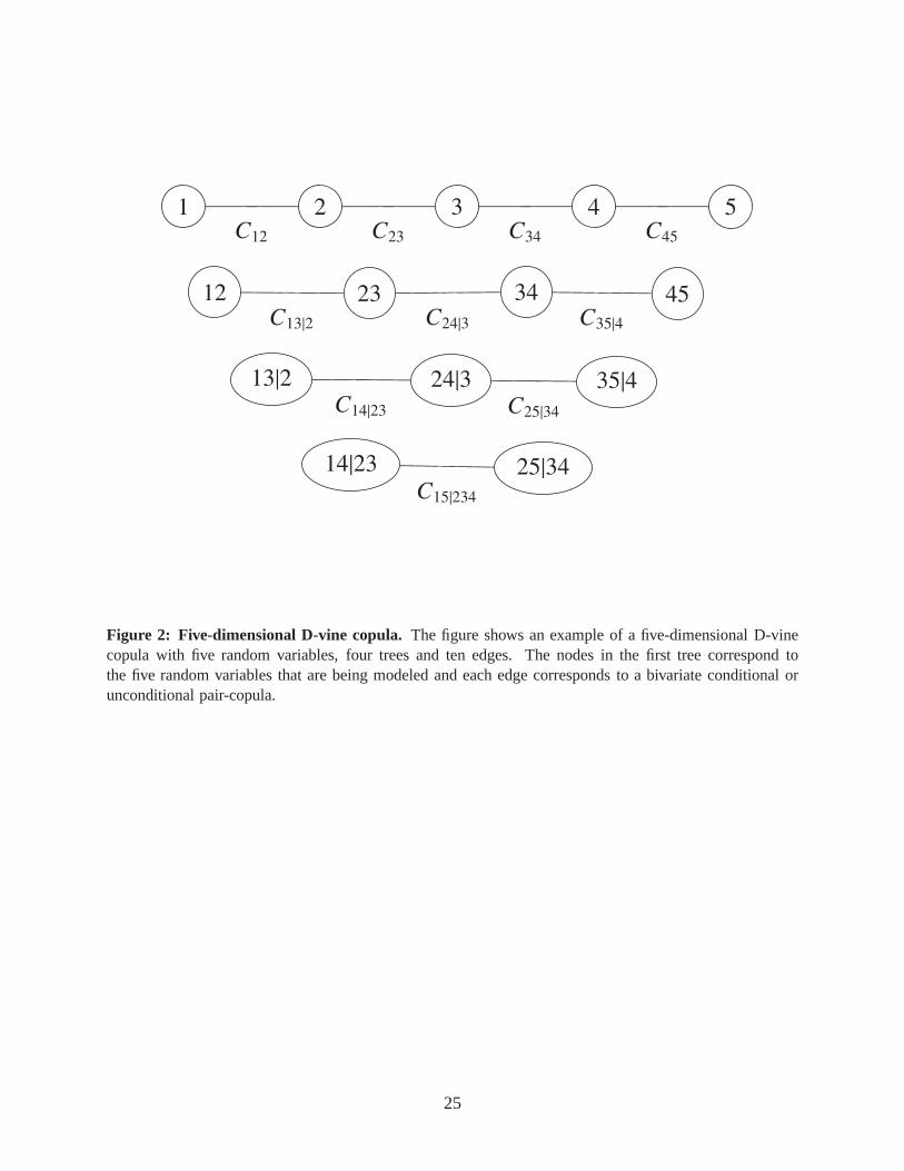
Examples of possible decompositions of a five-dimensional random vector via a C- and D-vine
copula are shown in Figure 1 and 2, respectively.
— insert Figures 1 and 2 here —
Fitting a vine copula model to a given dataset requires threeseparate steps. First, one needs to
select the tree structure of the vine model. For a C- or D-vine, this amounts to the selection of a
permutation of the indices1, . . . , d of the random variables. As such, for ad-dimensional random
vector their existd!/2 different C- and D-vines, respectively (see Aas et al., 2009).7 Once a per-
mutation has been chosen, the structure of the vine is fully specified. Second, the statistician has to
selectd(d−1)/2 bivariate pair-copulas from candidate copula families. Inthe last step, the param-
eters of the pair-copulas have to be estimated. To select theoptimal tree structure, Dißmann et al.
(forthcoming) propose a heuristic procedure in which the tree structure is chosen via a maximum
spanning tree algorithm that maximizes the sum of the absolute empirical Kendall’sτ of all possi-
ble variable pairs on a given level of the tree. For the selection of the parametric pair-copulas,
Brechmann and Czado (2012) and Dißmann et al. (forthcoming)propose a sequential heuristic
which selects the best fitting parametric copula family for each pair-copula based on the candi-
date copulas’ AIC values. Although this sequential selection of parametric pair-copulas using
AIC does not necessarily yield a globally optimal AIC value for the vine, Brechmann and Czado
(2012) show that this heuristic yields considerably betterresults than a selection algorithm based
on copula goodness-of-fit tests.8
In the following, we concentrate on the problem of selectingthe bivariate pair-copulas by
substituting them with smooth nonparametric estimates of the underlying (pairwise) dependence
structures. As a benchmark to our proposed nonparametric method, we employ the sequential
heuristic by Brechmann and Czado (2012) and Dißmann et al. (forthcoming). However, we expect
our nonparametric approach to improve on the heuristic benchmark for several reasons. First, the
nonparametric modeling of the pair-copulas eliminates completely the model risk of choosing an
incorrect parametric family for a given pair-copula. Second, Grønneberg and Hjort (2012) prove
7Choosing the best fitting tree structure manually thus quickly becomes unfeasible in higher dimension (seeDißmann et al., forthcoming).
8Results by Weiß (2011) and Grundke and Polle (2012) underline this finding. While Weiß (2011) shows thatgoodness-of-fit tests give only little guidance for choosing copulas when one is interested in forecasting quantiles inthe extreme tails of a joint distribution, the empirical results of Grundke and Polle (2012) cast additional doubt on theability of copula goodness-of-fit tests to identify stressed risk dependencies.
5
that the use of AIC as a model selection criterion is not correct in case rank-transformed pseudo-
observations are used (as is common in almost all applications of copulas in finance). Third,
as already hinted at by Dißmann et al. (forthcoming), the incorrect specification of the parametric
pair-copulas in the upper levels of a vine’s tree structure can lead to a propagation and amplification
of rounding errors causing the heuristic to become numerically unstable.
In the next subsection, we define and discuss Bernstein copulas which we use as smooth non-
parametric estimates of the pair-copulas in a vine model.
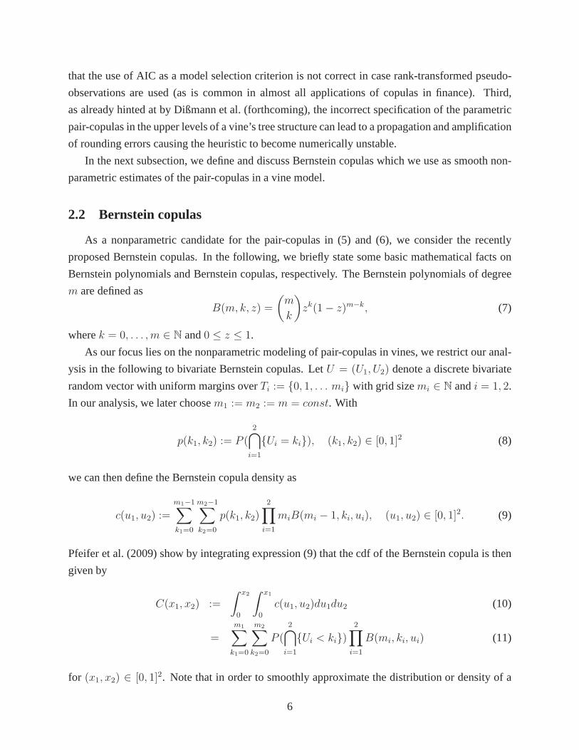
2.2 Bernstein copulas
As a nonparametric candidate for the pair-copulas in (5) and(6), we consider the recently
proposed Bernstein copulas. In the following, we briefly state some basic mathematical facts on
Bernstein polynomials and Bernstein copulas, respectively. The Bernstein polynomials of degree
m are defined as
B(m, k, z) =
(
m
k
)
zk(1− z)m−k, (7)
wherek = 0, . . . , m ∈ N and0 ≤ z ≤ 1.
As our focus lies on the nonparametric modeling of pair-copulas in vines, we restrict our anal-
ysis in the following to bivariate Bernstein copulas. LetU = (U1, U2) denote a discrete bivariate
random vector with uniform margins overTi := {0, 1, . . . mi} with grid sizemi ∈ N andi = 1, 2.
In our analysis, we later choosem1 := m2 := m = const. With
p(k1, k2) := P (
2⋂
i=1
{Ui = ki}), (k1, k2) ∈ [0, 1]2 (8)
we can then define the Bernstein copula density as
c(u1, u2) :=
m1−1∑
k1=0
m2−1∑
k2=0
p(k1, k2)2∏
i=1
miB(mi − 1, ki, ui), (u1, u2) ∈ [0, 1]2. (9)
Pfeifer et al. (2009) show by integrating expression (9) that the cdf of the Bernstein copula is then
given by
C(x1, x2) :=
∫ x2
0
∫ x1
0
c(u1, u2)du1du2 (10)
=
m1∑
k1=0
m2∑
k2=0
P (
2⋂
i=1
{Ui < ki})
2∏
i=1
B(mi, ki, ui) (11)
for (x1, x2) ∈ [0, 1]2. Note that in order to smoothly approximate the distribution or density of a
6
copula in (9) and (10), very high degrees for the Bernstein polynomials have to be chosen.
The Bernstein copula as defined above can then be used to approximate the empirical copula
process as defined, e.g., by Deheuvels (1979). To be precise,we approximate nonparametrically
the joint distribution ofU = (U1, U2) by using a bivariate sample{(Xi, Yi)}ni=1 of the underlying
copula of sizen. Let X(k) be thekth order statistic of the sample. The empirical copula of
Deheuvels (1979, 1981) is then defined as
Cn(x, y) =
Cn
(
i−1n, j−1
n
)
, i−1n
≤ x < in, j−1
n≤ y < j
n
1, x = y = 1,(12)
whereCn(x, y) =1n
∑nk=1 1{Xj≤X(i),Yj≤Y(i)}, Cn(0,
in) = Cn(
jn, 0) = 0 andCn(0,
in) = 0 (i, j =
1, 2, ..., n).
To fit the Bernstein copula to the sample from the empirical copula, we first need to calculate
the relative frequency of the observations in each target cell of a grid with given grid sizem. The
outcome of this is the contingency table[akl]k,l=1,...,m. Note, however, that the resulting marginals
of the data[akl] do not need to be uniformly distributed and that the resulting approximation could
therefore not be a copula. To circumvent this problem, Pfeifer et al. (2009) propose to transform
the contingency table[akl] into a (possibly suboptimal) new contingency table[xkl] with uniform
marginals via a Lagrange optimization approach yielding
xij = aij −a·jm
−ai·m
+2
m2for i, j = 1, . . . , m, (13)
where the index· denotes summation. Note that the quality of the Lagrange solution is reduced by
an increasing number of the sample sizen.9 We therefore chose to employ a different optimization
strategy to correct for the non-uniform distribution of themarginals.
Consequently, we calculate the approximation[xkl] to the contingency table[akl] by solving
the following optimization problem:
m∑
k=1
m∑
l=1
(xkl − akl)2 −→ min (14)
subject tom∑
k=1
xkj =m∑
l=1
xil =1
mand xij ≥ 0 for i, j = 1, . . . , m. (15)
To solve for the [xkl], we make use of the quadratic optimization algorithm of
Goldfarb and Idnani (1982, 1983). In preliminary tests, thefound solutions to this optimiza-
9In unreported results, the optimization strategy of Pfeifer et al. (2009) proved to yield only suboptimal results.
7
tion problem yielded significantly lower quadratic errors than the procedure initially proposed
by Pfeifer et al. (2009) thus confirming the need for a more refined optimization strategy.
To use Bernstein copulas as pair-copulas both in our simulation study and the empirical appli-
cation, we require efficient algorithms for simulating and evaluating the density and distribution of
a given vine copula. To this end, we adapt the algorithms initially proposed by Aas et al. (2009)
by substituting the parametric h-hunctions (i.e., the partial derivatives of the copula densities) in
these algorithms by the partial derivatives of the fitted bivariate Bernstein copulas.
3 Simulations
In this section, we illustrate the superiority of the smoothnonparametric vine model over the
sequential heuristic of Brechmann et al. (2012) and Dißmannet al. (forthcoming) for selecting the
pair-copulas in a vine parametrically. In particular, we are interested in the error of the approxima-
tions to a pre-specified true copula using both our smooth nonparametric model as well as a vine
model calibrated with parametric pair-copulas. The setup of our simulation study follows the pro-
cedure laid out in Shen et al. (2008), but differs in that way that we also consider a (heuristically
calibrated) parametric benchmark approximation to the true vine copula.
As a measure for the approximation error, we compare the pre-specified true pair-copulas of
the vine model with the parametric and nonparametric approximations and use the average squared
error (ASE) of the cdfs of all bivariate pair-copulas each taken atm1 ×m2 uniform grid points in
I2, i.e.,
ASE :=2
d(d− 1)
1
m1 ·m2
d(d−1)/2∑
i=1
m1∑
j=1
m2∑
k=1
(
Ci
(
j
m1 + 1,
k
m2 + 1
)
− Ci
(
j
m1 + 1,
k
m2 + 1
))2
(16)
whereCi is the cdf of a pre-specified pair-copula from which we simulate a random sample of size
n andCi is a (parametric or nonparametric) approximation to the pair-copulaCi computed on the
basis of the simulated random sample.
In the simulation study, we consider two sample sizesn = 200 andn = 500 to assess the de-
creasing effect of the sample size on the approximation error. Furthermore, we analyze the effect of
the type (C- or D-vine) as well as the dimensionality of the vine model on the approximation errors.
To be precise, we simulate random samples from vines of dimensiond = 3, 5, 6, 7, 11, 13. As the
dimension of the vine model increases, so does the number of variables one has to condition on in
the pair-copulas of the vine’s lower trees. The pair-copulas in the lower trees of the vine, however,
are generally more complex to model so that the accurate approximation of the pair-copulas on all
8

levels of the vine constitutes a considerable challenge to our nonparametric approximation.10 At
the same time, the curse of dimensionality could additionally complicate the approximation of the
pair-copulas thus making the comparison of our approximation for different dimensions a sensible
exercise. Finally, we expect the propagation and amplification of rounding errors to increase in
higher dimensions possibly leading to the numerical instability of the parametric heuristic.
As candidate parametric copula families from which the pair-copulas of the true vine models
are chosen, we use the Gaussian, Student’s t, Clayton, Gumbel, Survival Clayton, Survival Gum-
bel, the rotated Clayton copula (90 degrees) and the rotatedGumbel copula (90 degrees). The
pair-copulas as well as their respective parameters in eachsimulation are chosen randomly. For
each sample size, dimension and vine type, we simulate1, 000 random samples and approximate
the data with a vine copula using Bernstein copulas as pair-copulas. As we are only interested in
measuring the accuracy of the approximation of the pair-copulas, we calibrate our nonparametric
vine using the correct vine type as well as the correct tree structure. As a benchmark, we cali-
brate a second vine copula by using the sequential heuristicproposed by Brechmann and Czado
(2012) and Dißmann et al. (forthcoming). Furthermore, we also compute the fraction of time the
sequential procedure breaks down due to either the numerical instability of the evaluation of the
likelihood function and the parameter estimation or due to the ASE tending to infinity. The results
of the simulations are presented in Table 1.
— insert Table 1 here —
The results shown in Table 1 present several interesting insights into the finite sample prop-
erties of both the heuristically calibrated parametric andour proposed nonparametric vine copula
models. First, we can see from Table 1 that for lower dimensions (e.g.,d = 3 andd = 5) the ASE
of our nonparametric is considerably larger than for the parametric model calibrated by sequen-
tially selecting the pair-copulas based on AIC values. Withincreasing dimension of the random
vector, however, we can observe that the approximation error of the parametric model increases
disproportionately compared to our proposed nonparametric model. Furthermore, the nonpara-
metric model appears to be able to match the approximation error of the parametric approach for
dimensionsd = 13 and higher. Most importantly, the parametric modeling approach becomes
highly numerically unstable in higher dimensions. At the same time, our proposed nonparametric
vine with Bernstein pair-copulas is extremely reliable yielding acceptable approximations to the
true underlying dependence structure even for high-dimensional random vectors. The parametric
10This is one reason why Aas et al. (2009), Brechmann et al. (2012) and Dißmann et al. (forthcoming) propose tocapture as much dependence of the joint distribution that isto be modeled in the first trees of a vine model. If thesepair-copulas are modeled accurately, the remaining pair-copulas in the lower trees can then be truncated or simplified.Furthermore, the truncation and simplification of a vine on the lower levels of the vine’s tree limits the potentialpropagation of rounding errors.
9
approach, on the other hand, breaks down in approximately50% of all simulations for dimension
d = 13 and higher. In many of these cases, the bad approximation (ornumerical instability) of
the parametric approach was caused by the wrong selection ofseveral parametric families for the
pair-copulas in the vine model. Concerning the type of the vine copula model, we find no signifi-
cant differences between the average approximation errorsof the C- or D-vines. As expected, we
also find the average approximation error of both the parametric and nonparametric model to be
decreasing in the sample size used for estimating both models.
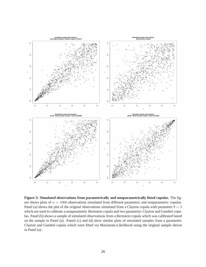
To further illustrate the finding that the nonparametric model improves on the accuracy of a
parametric vine especially in higher dimensions, we plot simulated samples from several paramet-
rically and nonparametrically fitted copulas in Figure 3 where we assume that the true underlying
dependence structure is given by a Clayton copula with parameterθ = 5. From this copula, we
simulate a random sample of sizen = 500 and fit both a nonparametric Bernstein copula as well
as a parametric Clayton and Gumbel copula via Maximum-Likelihood to the data. From all three
fitted copulas, we again simulate a random sample and comparethe plots of the simulated obser-
vations with the original sample.
— insert Figure 3 here —
The plots in Panels (a) and (b) in Figure 3 show how the Bernstein copula approximately cap-
tures the lower tail dependence of the original sample shownin Panel (a). The plot of the Bernstein
copula in Panel (b) also shows, however, that the nonparametric approximation of the data sam-
ple coincides with a loss in information on the tail behaviour of the true underlying dependence
structure. At the same time, Panel (c) underlines the notionthat the nonparametric model is not
superior to a parametric model in which the parametric copula family has been chosen correctly.
If, however, the parametric copula familiy is chosen incorrectly like it is shown in Panel (d), the
wrong selection of the parametric copula family can cause considerable approximation errors and
a severely inaccurate modeling of the underlying tail dependence. Given no prior information on
the parametric copula familiy, the nonparametric Bernstein copula model clearly improves on the
fit of an inaccurately fitted parametric model. The nonparametric modeling of the pair-copulas
thus seems to be a sensible approach especially when the number of pair-copulas that need to be
selected from candidate parametric copula families increases (i.e., with increasing dimension).
4 Empirical study
4.1 Methodology
The purpose of our empirical study is to investigate the superiority of the proposed smooth
nonparametric vine copula models over the competing calibration strategy based on a sequential
10
selection of parametric pair-copulas via AIC with regard tothe accurate forecasting of a portfo-
lio’s VaR. The simulation study presented in the previous section has highlighted the finding that
our vine model with smooth nonparametric pair-copulas is especially well-suited for dependence
modeling in higher dimensions as the selection of parametric pair-copulas becomes numerically
unstable due to error propagation and amplification. For low-dimensional problems, the heuristic
selection of parametric copulas, however, seems to outperform our nonparametric approach with
respect to the ASE of the vine copula’s approximation. To show that our nonparametric model
matches the results of the parametric heuristic even for low-dimensional problems, we concentrate
in our empirical analysis on the VaR forecasts of a five-dimensional portfolio.
Financial data are usually characterized by the presence ofboth conditional heteroscedas-
ticity and asymmetric dependence in the log returns on financial returns. Therefore, we fol-
low the vast majority of studies on copula models for VaR-estimation (Jondeau and Rockinger,
2006; Fantazzini, 2009; Ausin and Lopes, 2010; Hafner and Reznikova, 2010) and employ stan-
dard GARCH(1,1)-models with Student’s t-distributed innovations to model the marginal be-
haviour of our data. Although different specifications of the GARCH model are also possible,
results found by Hansen and Lunde (2005) suggest that the choice of the order of a GARCH model
is only of little importance for the model’s forecasting accuracy.
Throughout the empirical study, we consider continuous logreturns on financial assets with
pricesPt (t = 0, 1, . . . , T ). The assets’ log returnsRt are defined byRt := log(Pt/Pt−1) for
t ≥ 1. Our focus lies on modeling the joint distribution of thed assets, i.e., the joint distribution of
the returnsRt1, . . . , Rtd.
The marginal behaviour of the assets is modeled by the use of GARCH(1,1)-models with t-
distributed innovations. The marginal model is then given by
Rtj = µj + σtjZtj , (17)
σ2tj = α0j + α1jR
2t−1,j + βjσ
2t−1,j , j = 1, . . . , d; t = 1, . . . , T, (18)
with independent and identically t-distributed innovationsZtj. The dependence structure between
thed assets is introduced into the model by assuming the vectorZt = (Zt1, . . . , Ztd) (t = 1, . . . , T )
of the innovations to be jointly distibuted under ad-dimensional copulaC with
FZ(z;ν1, . . . ,νd,ω|Ft−1) = C [F1(z1;ν1|Ft−1), . . . , Fd(zd;νd|Ft−1);ω] (19)
whereν1, . . . ,νd are the parameter vectors of the innovations,C is a copula andω is a vector of
copula parameters (in case of the parametric model, otherwiseω is simply empty).
The parameters of the univariate GARCH-models are estimated via Quasi-Maximum Likeli-
hood Estimation. For the estimation of both the nonparametric vine model as well as the para-
11
metric model calibrated by using the pair-copulas’ AIC values, we make use of rank-transformed
pseudo-observations rather than the original sample as input data.11 As the main results for copu-
las only hold for i.i.d. samples, we use the parameter estimates for the univariate GARCH models
and transform the original observations into standardizedresiduals to yield (approximately) i.i.d.
observations before computing the pseudo-observations (Dias and Embrechts, 2009).
In our empirical application, we consider an equally-weighted five-dimensional portfolio with
returnsRp,t = d−1∑d
j=1Rtj . The results from our simulation study underline the findingthat our
proposed vine copula model with Bernstein pair-copulas, onaverage, yields a better approximation
to the empirical copula than the heuristically calibrated parametric model especially in higher
dimensions. However, the parametric copula vine model could still outperform our proposed model
w.r.t. the forecasting accuracy in low dimensions. In our empirical application, we therefore restrict
our analysis to a portfolio consisting of five assets to additionally illustrate the nonparametric
Bernstein vine copula model’s superiority for low-dimensional problems.
To forecast the portfolio returns, we employ the algorithm presented in the study by
Nikoloulopoulos et al. (2011) initially proposed for in-sample forecasting which was extended to
out-of-sample forecasting by Weiß (2012).
The aim of the algorithm is the computation of a one-day-ahead forecast for the portfolio re-
turnRp,t via Monte Carlo simulation. In a first step,K = 10, 000 observationsu(k)T+1,1, . . . , u(k)T+1,d
(k = 1, . . . , K) from the fitted (parametric or nonparametric) vine copula are simulated. Us-
ing the quantile function of the fitted marginal Student’s t distributions, the simulated vine cop-
ula observations are then transformed into observationsz(k)T+1,j from the joint distribution of the
innovations. In the next step, the simulated innovations are transformed into simulated returns
R(k)T+1,j = µj + σT+1,jz
(k)T+1,j whereσT+1,j andµj are the forecasted conditional volatility and mean
values from the previously fitted marginal GARCH models. TheMC-simulated forecasts of the
portfolio return is then simply given byR(k)T+1,p = d−1
∑dj=1R
(k)T+1,j . Sorting the simulated portfo-
lio returns for a given day in the forecasting period and taking the empirical one-dayα percentile
then yields the forecastedα%-VaR.
To backtest the results of our forecasting, we employ the test of conditional cover-
age proposed by Christoffersen (1998) as well as two duration-based tests discussed in
Christoffersen and Pelletier (2004a).12
11For a comparative study on the finite sample properties of different ML-based estimators for copulas, seeKim et al. (2007). The authors show that absent any information on the true distribution of the marginals, statisti-cal inferences should be based on rank-transformed pseudo-observations.
12See Berkowitz et al. (2011) for an excellent review of different methods for backtesting Value-at-Risk forecasts.A comparison of different backtests can be found in the recent study by Escanciano and Pei (2012).
12
All three backtests are based on the hit sequence of VaR-exceedances which is defined by
ht,α :=
{
1, if Rp,t <VaRα(Rp,t)|Ft−1
0, otherwise.
with t being the time subscript andFt−1 being the set of available information. The test of condi-
tional coverage by Christoffersen (1998) and Christoffersen and Pelletier (2004a) jointly tests for
the correct number of VaR-exceedances (unconditional coverage) and the serial independence of
the violations over the complete out-of-sample (independence).13 Under the null hypothesis of
a correct number of VaR-exceedances that are independent over time, the hit sequence is simply
distributed as (Christoffersen and Pelletier, 2004a)
ht,α ∼ i.i.d. Bernoulli(α).
Then, letP be the length of the out-of-sample,P1 be the number of VaR-exceedances andP0 be the
number of days on which the daily VaR forecast was not exceeded, respectively (and consequently
P = P1 + P0). The likelihood function for the i.i.d.Bernoulli hit sequence with unknown
parameterπ1 is
L(ht,α, π1) = πP11 (1− π1)
P−P1 (20)
and the Maximum-Likelihood estimate ofπ1 is simply given byπ1 = P1/P . The test of uncondi-
tional coverage is then given by a likelihood ratio test based on
LRUC = −2 (lnL(ht,α, π1)− lnL(ht,α, α)) . (21)
To test the hypothesis of independently distributed hits, the hit sequence is assumed to follow a
first order Markov sequence with switching probability matrix
Π =
[
1− π01 π01
1− π11 π11
]
(22)
with πij being the probability of ani on dayt − 1 being followed by aj on the next dayt and
i, j ∈ {1; 0}. Using the likelihood function
L(ht,α, π01, π11) = (1− π01)P0−P01πP01
01 (1− π11)P1−P11πP11
11 .
13The test of unconditional coverage has been implicitly incorporated in the Basel Accord for determining cap-ital requirements for market risks, see Basel Committee on Banking Supervision (1996). Consequently, it has sincebecome an industry standard in market risk management, see,e.g., Escanciano and Pei (2012).
13

wherePij is the number of observations inht,α where aj follows ani andi, j ∈ {1; 0} and the
ML-estimatesπ01 = P01/P0 and π11 = P11/P1, the likelihood ratio test of the independence of
hits is given by
LRind = 2 (lnL(ht,α, π01, π11)− lnL(ht,α, π1)) . (23)
Both tests are then combined viaLRCC = LRUC + LRind to yield the test of conditional cov-
erage. We note here that we do not rely on the asymptotic Chi-squared distribution of the test
statistic which is used, e.g., in the study by Hsu et al. (2011). Although easy to implement, p-
values derived under the assumption of the test statistic following a Chi-squared distribution are
usually incorrect due to the generally low sample sizes whenusing hit sequences. Instead, we
follow Christoffersen and Pelletier (2004a) in generatingapproximate p-values via Monte Carlo-
simulation.
As an alternative to the test of conditional coverage, Christoffersen and Pelletier (2004a) pro-
pose backtests based on the durations between VaR-exceedances. Then, let
Di = ti − ti−1 (24)
be the duration of time (in trading days) between two subsequent VaR-exceedances whereti is the
time of theith VaR-exceedance. Under the null hypothesis of a correctlyspecified VaR model,
we would expect the process of no-hit durations to have no memory and mean1/α. Conse-
quently, the processD of durations should follow an exponential distribution with fexp(D;α) =
α exp (−αD).14 As an alternative hypothesis, Christoffersen and Pelletier (2004a) propose to use
the Weibull distribution for the processD with fW (D; a, b) = abbDb−1 exp(
−(aD)b)
which nests
the exponential distribution from the null hypothesis forb = 1.
Although this test potentially captures higher order dependence in the hit sequenceht,α, the
information from the temporal ordering of the no-hit durations is not exploited in the backtest. As
a remedy, Christoffersen and Pelletier (2004a) propose a conditional duration-based test based on
the Exponential Autoregressive Conditional Duration (EACD) model of Engle and Russell (1998).
In the standard EACD (1,0) model, the conditional expected durationEi−1(Di) is assumed to
follow the process
Ei−1(Di) ≡ ψi = ω + βDi−1. (25)
Again assuming an underlying exponential density with meanequal to one in the null hypothesis,
14See Christoffersen and Pelletier (2004a) for details of thebacktest and the motivation for using a continuousdistribution for the discrete processD.
14
the conditional distribution of the duration is is given by
fEACD (Di|ψi) =1
ψiexp
(
−Di
ψi
)
. (26)
The null hypothesis of independent no-hit durations is thengiven byH0 : β = 0.
4.2 Data
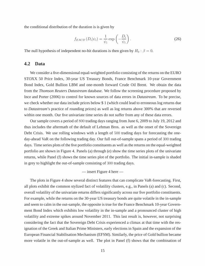
We consider a five-dimensional equal-weighted portfolio consisting of the returns on the EURO
STOXX 50 Price Index, 30-year US Treasury Bonds, France Benchmark 10-year Government
Bond Index, Gold Bullion LBM and one-month forward Crude OilBrent. We obtain the data
from theThomson Reuters Datastreamdatabase. We follow the screening procedure proposed by
Ince and Porter (2006) to control for known sources of data errors inDatastream. To be precise,
we check whether our data include prices below $ 1 (which could lead to erroneous log returns due
to Datastream’s practice of rounding prices) as well as log returns above 300% that are reversed
within one month. Our five univariate time series do not suffer from any of these data errors.
Our sample covers a period of800 trading days ranging from June 6, 2009 to July 19, 2012 and
thus includes the aftermath of the default of Lehman Bros. aswell as the onset of the Sovereign
Debt Crisis. We use rolling windows with a length of500 trading days for forecasting the one-
day-ahead VaR on the following trading day. Our full out-of-sample spans a period of300 trading
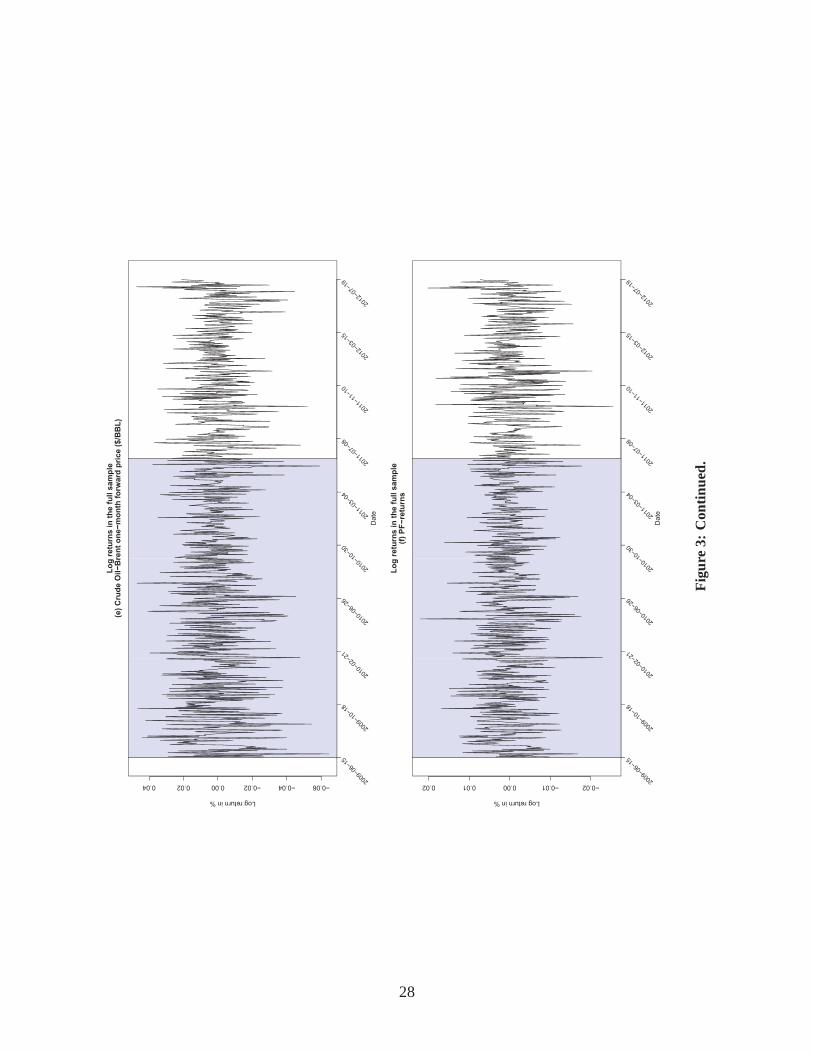
days. Time series plots of the five portfolio constituents aswell as the returns on the equal-weighted
portfolio are shown in Figure 4. Panels (a) through (e) show the time series plots of the univariate
returns, while Panel (f) shows the time series plot of the portfolio. The initial in-sample is shaded
in grey to highlight the out-of-sample consisting of300 trading days.
— insert Figure 4 here —
The plots in Figure 4 show several distinct features that cancomplicate VaR-forecasting. First,
all plots exhibit the common stylized fact of volatility clusters, e.g., in Panels (a) and (c). Second,
overall volatility of the univariate returns differs significantly across our five portfolio constituents.
For example, while the returns on the 30-year US treasury bonds are quite volatile in the in-sample
and seem to calm in the out-sample, the opposite is true for the France Benchmark 10-year Govern-
ment Bond Index which exhibits low volatility in the in-sample and a pronounced cluster of high
volatility and extreme spikes around November 2011. This last result is, however, not surprising
considering the fact that the Sovereign Debt Crisis experienced a climax at that time with the res-
ignation of the Greek and Italian Prime Ministers, early elections in Spain and the expansion of the
European Financial Stabilisation Mechanism (EFSM). Similarly, the price of Gold bullion became
more volatile in the out-of-sample as well. The plot in Panel(f) shows that the combination of
15
the five individual assets produces a portfolio which exhibits several phases of both high and low
volatility as well as sudden extreme spikes in the portfolio’s log returns.
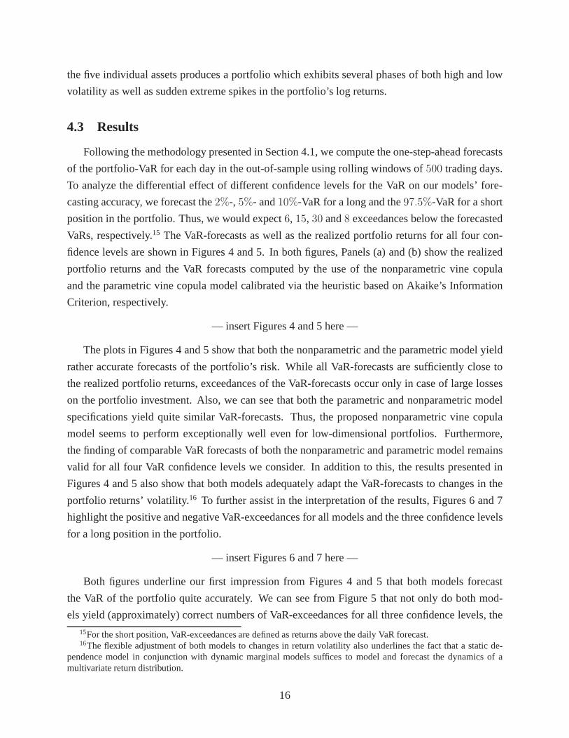
4.3 Results
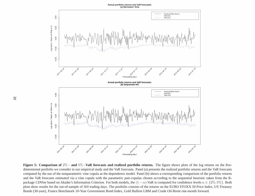
Following the methodology presented in Section 4.1, we compute the one-step-ahead forecasts
of the portfolio-VaR for each day in the out-of-sample usingrolling windows of500 trading days.
To analyze the differential effect of different confidence levels for the VaR on our models’ fore-
casting accuracy, we forecast the2%-, 5%- and10%-VaR for a long and the97.5%-VaR for a short
position in the portfolio. Thus, we would expect6, 15, 30 and8 exceedances below the forecasted
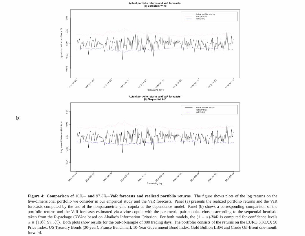
VaRs, respectively.15 The VaR-forecasts as well as the realized portfolio returnsfor all four con-
fidence levels are shown in Figures 4 and 5. In both figures, Panels (a) and (b) show the realized
portfolio returns and the VaR forecasts computed by the use of the nonparametric vine copula
and the parametric vine copula model calibrated via the heuristic based on Akaike’s Information
Criterion, respectively.
— insert Figures 4 and 5 here —
The plots in Figures 4 and 5 show that both the nonparametric and the parametric model yield
rather accurate forecasts of the portfolio’s risk. While all VaR-forecasts are sufficiently close to
the realized portfolio returns, exceedances of the VaR-forecasts occur only in case of large losses
on the portfolio investment. Also, we can see that both the parametric and nonparametric model
specifications yield quite similar VaR-forecasts. Thus, the proposed nonparametric vine copula
model seems to perform exceptionally well even for low-dimensional portfolios. Furthermore,
the finding of comparable VaR forecasts of both the nonparametric and parametric model remains
valid for all four VaR confidence levels we consider. In addition to this, the results presented in
Figures 4 and 5 also show that both models adequately adapt the VaR-forecasts to changes in the
portfolio returns’ volatility.16 To further assist in the interpretation of the results, Figures 6 and 7
highlight the positive and negative VaR-exceedances for all models and the three confidence levels
for a long position in the portfolio.
— insert Figures 6 and 7 here —
Both figures underline our first impression from Figures 4 and5 that both models forecast
the VaR of the portfolio quite accurately. We can see from Figure 5 that not only do both mod-
els yield (approximately) correct numbers of VaR-exceedances for all three confidence levels, the
15For the short position, VaR-exceedances are defined as returns above the daily VaR forecast.16The flexible adjustment of both models to changes in return volatility also underlines the fact that a static de-
pendence model in conjunction with dynamic marginal modelssuffices to model and forecast the dynamics of amultivariate return distribution.
16
exceedances also seem to occur randomly in time. Most importantly, however, our proposed non-
parametric vine copula model with GARCH margins easily matches the heuristically calibrated
parametric vine w.r.t. the accuracy of VaR-forecasting even for a relatively low-dimensional port-
folio. To further substantiate this finding, we perform three formal backtests on the results of both
the parametric and nonparametric vine models. The results of the three backtests are presented in
Table 2.
— insert Table 2 here —
The backtesting results stress our finding that both models yield comparable results. For ex-
ample, all but one VaR models cannot be rejected at the99% confidence level based on the test of
conditional coverage. Although the results of the unconditional duration-based backtest imply a
significantly worse forecasting accuracy of both models, the p-values for both the nonparametric
and the parametric model are comparable for different confidence levels of the VaR. This indicates
that neither model outperforms the other one based on our second backtest. If we use the condi-
tional duration-based test of Christoffersen and Pelletier (2004b) instead, none of the VaR-models
is rejected. Turning to the number of VaR-exceedances, the results of our nonparametric vine cop-
ula model are slightly better for the5%-VaR than those of the parametric benchmark while the
opposite is true for the (for most practical uses too optimistic and thus unsuitable)10%-VaR.
Our backtesting results indicate that both models yield acceptable VaR-forecasts for a relatively
low-dimensional portfolio. One could conclude from this finding that in general using our non-
parametric vine copula model does not yield significantly better VaR-forecasts. However, one has
to keep in mind that our empirical analysis was deliberatelyaimed at testing the hypothesis that the
nonparametric model yields accurate VaR-forecasts even inlower dimensions. In unreported tests
of high-dimensional portfolios, the parametric benchmarksuffered from the same numerical insta-
bility that was also observed in our simulation study. At thesame time, our nonparametric model
produced accurate VaR-forecasts in a numerically stable fashion even for high-dimensional port-
folios when the parametric benchmark had either broken downor produced woefully inaccurate
VaR-forecasts.
5 Summary
In this paper, we propose to model the pair-copulas in a vine copula model nonparametrically
by the use of Bernstein copulas. Our proposed model has the advantage of a significantly reduced
model risk as it avoids the error-prone selection of pair-copulas from candidate parametric copula
families. In contrast to previous studies on the use of discrete empirical copulas as pair-copulas, our
proposed use of Bernstein copulas has the additional advantage that the building blocks in a vine
17

model are approximated by smooth functions from which one can easily simulate random samples.
We test the approximation error of the smooth nonparametricBernstein vine copula model against a
parametric benchmark calibrated by the use of a sequential heuristic based on AIC. The superiority
of our proposed model is exemplified in an empirical risk management application.
The results we find in our simulation study show that for low-dimensional problems, the para-
metric modeling approach outperforms our proposed nonparametric approach only marginally.
However, the differences in the approximation error quickly vanish for higher dimensions with
both models yielding comparable average approximations errors for dimensionsd = 13 and higher.
At the same time, our proposed nonparametric vine copula model does not suffer from numerical
instability and error propagation which plagues the parametric benchmark due to an increasing
number of wrongly selected parametric pair-copulas.
In the empirical risk management application, we test whether the differences in the average
approximation error of the parametric and nonparametric vine copula models cause significant dif-
ferences in both models’ accuracy of forecasting the VaR of alow-dimensional asset portfolio. The
results of our analysis show that even in lower dimensions (d = 5), our nonparametric vine cop-
ula model yields VaR-forecasts that cannot be rejected by several different formal backtests. The
proposed nonparametric vine copula model thus seems to match the (good) results of a parametric
vine copula model in lower dimensions and significantly outperforms this benchmark in higher
dimensions.
A natural extension of our model would be to consider more sophisticated smooth approxi-
mations of the empirical copula. Cubic B-splines and non-uniform rational B-splines (NURBS)
appear as natural candidates for this job. While Bernstein copulas have been shown to be good
smooth nonparametric replacements for parametric pair-copulas, spline copulas should yield even
better approximations while at the same time yielding numerically stable vine model calibrations
as well. We intend to analyze the suitability of spline copulas in vine models in future research.
18

References
AAS, K. AND D. BERG (2009): “Models for construction of multivariate dependence - a compar-ison study,”European Journal of Finance, 15, 639–659.
AAS, K., C. CZADO, A. FRIGESSI, AND H. BAKKEN (2009): “Pair-Copula Constructions ofMultiple Dependence,”Insurance: Mathematics and Economics, 44, 182–198.
AUSIN, M. AND H. LOPES(2010): “Time-varying joint distribution through copulas,” Computa-tional Statistics and Data Analysis, 54(11), 2383–2399.
BASEL COMMITTEE ON BANKING SUPERVISION (1996): “Supervisory framework for the useof backtesting in conjunction with the internal models approach to market risk capital require-ments,” Tech. rep., Bank of International Settlements.
BEDFORD, T. AND R. COOKE (2001): “Probability density decomposition for conditionally de-pendent random variables modeled by vines,”Annals of Mathematics and Artificial Intelligence,32, 245–268.
——— (2002): “Vines - A New Graphical Model for Dependent Random Variables,”Annals ofStatistics, 30, 1031–1068.
BERKOWITZ, J., P. CHRISTOFFERSEN, AND D. PELLETIER (2011): “Evaluating Value-at-Riskmodels with desk-level data,”Management Science, 57, 2213–2227.
BRECHMANN, E. AND C. CZADO (2012): “Risk management with high-dimensional vine copu-las: An analysis of the Euro Stoxx 50,”working paper.
BRECHMANN, E., C. CZADO, AND K. AAS (2012): “Truncated Regular Vines in High Dimen-sions with Applications to Financial Data,”Canadian Journal of Statistics, 40(1), 68–85.
CHAN , J. C.AND D. P. KROESE(2012): “Efficient estimation of large portfolio loss probabilitiesin t-copula models,”European Journal of Operational Research, 205, 361367.
CHRISTOFFERSEN, P. (1998): “Evaluating Interval Forecasts,”International Economic Reviewe,39, 841–862.
CHRISTOFFERSEN, P. AND D. PELLETIER (2004a): “Backtesting Value-at-Risk: A Duration-Based Approach,”Journal of Financial Econometrics, 2, 84–108.
——— (2004b): “Backtesting Value-at-Risk: A duration-based approach,”Journal of FinancialEconometrics, 2, 84–108.
DEHEUVELS, P. (1979): “La fonction de dependance empirique et ses proprietes - Un test nonparametrique d’independance,”Academie Royale de Belgique - Bulletin de la Classe des Sci-ences - 5e Serie, 65, 274–292.
——— (1981): “An asymptotic decomposition for multivariatedistribution-free tests of indepen-dence,”J. Multivariate Anal., 11, 102–113.
19
DIAS, A. AND P. EMBRECHTS (2009): “Testing for structural changes in exchange rates’depen-dence beyond linear correlation,”The European Journal of Finance, 15, 619–637.
DIERS, D., M. ELING , AND S. MAREK (2012): “Dependence modeling in non-life insuranceusing the Bernstein copula,”Insurance: Mathematics and Economics, 50, 430–436.
DISSMANN, J., E. BRECHMANN, C. CZADO, AND D. KUROWICKA (forthcoming): “Selectingand estimating regular vine copulae and application to financial returns,”Computational Statis-tics and Data Analysis.
EMBRECHTS, P., A. MCNEIL , AND D. STRAUMANN (2002): “Correlation and dependence inrisk management: properties and pitfalls,” inRisk Management: Value at Risk and Beyond, ed.by M. Dempster, Cambridge University Press, Cambridge, 176–223.
ENGLE, R. AND J. RUSSELL (1998): “Autoregressive Conditional Duration: A New ModelforIrregularly Spaced Transaction Data,”Econometrica, 66, 1127–1162.
ESCANCIANO, J. C.AND P. PEI (2012): “Pitfalls in backtesting Historical Simulation VaR mod-els,” Journal of Banking and Finance, 36, 2233–2244.
FANTAZZINI , D. (2009): “Market Risk Management for Emerging Markets: Evidence from theRussian Stock Market,” inEmerging markets: Performance, analysis and innovation, ed. byG. Gregoriou, Chapman and Hall / CRC Finance, 533–554.
FISCHER, M., C. KOCK, S. SCHLUTER, AND F. WEIGERT (2009): “An empirical analysis ofmultivariate copula model,”Quantitative Finance, 7, 839–854.
GENEST, C., M. GENDRON, AND M. BOURDEAU-BRIEN (2009a): “The advent of copulas infinance,”European Journal of Finance, 15, 609–618.
GENEST, C., B. REMILLARD , AND D. BEAUDOIN (2009b): “Goodness-of-fit tests for copulas:A review and a power study,”Insurance: Mathematics and Economics, 44, 199–213.
GOLDFARB, D. AND A. IDNANI (1982): “Dual and Primal-Dual Methods for Solving StrictlyConvex Quadratic Programs,” Springer Verlag, Berlin, 226–239.
——— (1983): “A numerically stable dual method for solving strictly convex quadratic programs,”Mathematical Programming, 27, 1–33.
GRØNNEBERG, S. AND N. L. HJORT (2012): “The Copula Information Criterion,”ScandinavianJournal of Statistics, forthcoming.
GRUNDKE, P. AND S. POLLE (2012): “Crisis and risk dependencies,”European Journal of Oper-ational Research, 223, 518–528.
HAFNER, C. AND O. REZNIKOVA (2010): “Efficient estimation of a semiparametric dynamiccopula models,”Computational Statistics and Data Analysis, 54(11), 2069–2627.
HANSEN, P. AND A. LUNDE (2005): “A Forecast Comparison of Volatility Models: Does Any-thing Beat a GARCH(1,1)?”Journal of Applied Econometrics, 20, 873–889.
20
HOBÆK-HAFF, I. AND J. SEGERS (2012): “Non-parametric estimation of pair-copula construc-tions with the empirical pair-copula,”Working Paper, January 2012.
HSU, C., C. HUANG, AND W. CHIOU (2011): “Effectiveness of Copula-Extreme Value Theoryin Estimating Value-at-Risk: Empirical Evidence from Asian Emerging Markets,”Review ofQuantitative Finance and Accounting, Forthcoming.
INCE, O. AND R. PORTER (2006): “Individual Equity Return Data From Thomson Datastream:Handle With Care!”Journal of Financial Research, 29, 463–479.
JOE, H. (1996): “Families of m-variate distributions with given margins and m(m-1)/2 bivari-ate dependence parameters,” inDistributions with Fixed Marginals and Related Topics, ed. byL. Rschendorf, B. Schweizer, and M. Taylor, Hayward, CA: IMSLecture Notes - MonographSeries, 120–141.
——— (1997):Multivariate Models and Dependence Concepts, Chapman & Hall, London.
JONDEAU, E. AND M. ROCKINGER (2006): “The copula-GARCH model of conditional depen-dencies: An international stock market application,”Journal of International Money and Fi-nance, 25(5), 827–853.
K IM , G., M. SILVAPULLE , AND P. SILVAPULLE (2007): “Comparison of semiparametric andparametric methods for estimating copulas,”Computational Statistics and Data Analysis, 51,2836–2850.
KOLE, E., K. KOEDIJK, AND M. VERBEEK (2007): “Selecting Copulas for Risk Management,”Journal of Banking & Finance, 31, 2405–2423.
KULPA, T. (1999): “On approximation of copulas,”International Journal of Mathematics andMathematical Sciences, 22, 259–269.
KUROWICKA, D. (2010): “Optimal truncation of vines,” inDependence Modeling: Handbook onVine Copulae, ed. by D. Kurowicka and H. Joe, World Scientific Publishing Co.
NIKOLOULOPOULOS, A., H. JOE, AND H. L I (2011): “Vine copulas with asymmetric tail de-pendence and applications to financial return data,”Computational Statistics and Data Analysis,forthcoming.
PFEIFER, D., D. STRASSBURGER, AND J. PHILIPPS (2009): “Modelling and simulation of de-pendence structures in nonlife insurance with Bernstein copulas,”Working Paper, Carl von Ossi-etzky University, Oldenburg.
SANCETTA, A. AND S. SATCHELL (2004): “The Bernstein copula and its applications to modelingand approximations of multivariate distributions,”Econometric Theory, 20, 1–38.
SHEN, X., Y-ZHU, AND L. SONG (2008): “Linear B-spline copulas with applications to nonpara-metric estimation of copulas,”Computational Statistics and Data Analysis, 52, 3806–3819.
21
WEISS, G. (2011): “Are Copula-GoF-tests of any practical use? Empirical evidence for stocks,commodities and FX futures,”The Quarterly Review of Economics and Finance, 51(2), 173–188.
——— (2012): “Copula-GARCH vs. Dynamic Conditional Correlation - an empirical study onVaR and ES forecasting accuracy,”Review of Quantitative Finance and Accounting, forthcom-ing.
WHELAN , N. (2004): “Sampling from Archimedean copulas,”Quantitative Finance.
YEA, W., C. LIUB, AND B. M IAOA (2012): “Measuring the subprime crisis contagion: Evidenceof change point analysis of copula functions,”European Journal of Operational Research, 222,96–103.
22

Figures and Tables
23

1
23
5
4
12
13
15
14
23|1
24|1
25|1
34|12 35|12
C12
C13
C15
C14
C23|1
C25|1
C24|1
C34|12
C35|12
C45|123
Figure 1: Five-dimensional C-vine copula. The figure shows an example of a five-dimensional C-vinecopula with five random variables, four trees and ten edges. The nodes in the first tree correspond tothe five random variables that are being modeled and each edgecorresponds to a bivariate conditional orunconditional pair-copula.
24
1 2 3 4 5
12 23 34 45
13|2 24|3 35|4
14|23 25|34
C12 C23 C34 C45
C13|2 C24|3 C35|4
C14|23 C25|34
C15|234
Figure 2: Five-dimensional D-vine copula.The figure shows an example of a five-dimensional D-vinecopula with five random variables, four trees and ten edges. The nodes in the first tree correspond tothe five random variables that are being modeled and each edgecorresponds to a bivariate conditional orunconditional pair-copula.
25
0.0 0.2 0.4 0.6 0.8 1.0
0.0
0.2
0.4
0.6
0.8
1.0
u
v
Simulated copula observations:(a) Original Sample: Clayton copula, Theta=5
0.0 0.2 0.4 0.6 0.8 1.0
0.0
0.2
0.4
0.6
0.8
1.0
u
v
Simulated copula observations:(b) Bernstein copula
0.0 0.2 0.4 0.6 0.8 1.0
0.0
0.2
0.4
0.6
0.8
1.0
u
v
Simulated copula observations:(c) ML−fitted Clayton copula, Theta=5.185086
0.0 0.2 0.4 0.6 0.8 1.0
0.0
0.2
0.4
0.6
0.8
1.0
u
v
Simulated copula observations:(d) ML−fitted Gumbel copula, Theta=3.479291
Figure 3: Simulated observations from parametrically and nonparametrically fitted copulas. The fig-ure shows plots ofn = 1000 observations simulated from different parametric and nonparametric copulas.Panel (a) shows the plot of the original observations simulated from a Clayton copula with parameterθ = 5which are used to calibrate a nonparametric Bernstein copula and two parametric Clayton and Gumbel copu-las. Panel (b) shows a sample of simulated observations froma Bernstein copula which was calibrated basedon the sample in Panel (a). Panels (c) and (d) show similar plots of simulated samples from a parametricClayton and Gumbel copula which were fitted via Maximum-Likelihood using the original sample shownin Panel (a).
26

−0.0
50.0
00.0
50.1
0
Log r
etu
rn in %
2009
−06−
15
2009
−10−
18
2010
−02−
21
2010
−06−
26
2010
−10−
30
2011
−03−
04
2011
−07−
08
2011
−11−
10
2012
−03−
15
2012
−07−
19
(a) EURO STOXX 50 Price IndexLog returns in the full sample
Date
−0.0
10
−0.0
05
0.0
00
0.0
05
0.0
10
Log r
etu
rn in %
2009
−06−
15
2009
−10−
18
2010
−02−
21
2010
−06−
26
2010
−10−
30
2011
−03−
04
2011
−07−
08
2011
−11−
10
2012
−03−
15
2012
−07−
19
(b) US Treasury Bonds (30−Year)Log returns in the full sample
Date
−0.0
2−
0.0
10.0
00.0
10.0
2
Log r
etu
rn in %
2009
−06−
15
2009
−10−
18
2010
−02−
21
2010
−06−
26
2010
−10−
30
2011
−03−
04
2011
−07−
08
2011
−11−
10
2012
−03−
15
2012
−07−
19
(c) France Benchmark 10−Year Government Bond Index (Clean Price)Log returns in the full sample
Date−
0.0
6−
0.0
4−
0.0
20.0
00.0
20.0
4
Log r
etu
rn in %
2009
−06−
15
2009
−10−
18
2010
−02−
21
2010
−06−
26
2010
−10−
30
2011
−03−
04
2011
−07−
08
2011
−11−
10
2012
−03−
15
2012
−07−
19
(d) Gold Bullion LBM ($/Troy Ounce)Log returns in the full sample
Date
Figure 4: Time series plots of log returns in the full sample.The figure shows plots of the log returns on the EURO STOXX 50 Price Index inPanel (a), US Treasury Bonds (30-year) in Panel (b), France Benchmark 10-Year Government Bond Index (Clean Price) in Panel (c), Gold BullionLBM ($/Troy Ounce) in Panel (d), Crude Oil-Brent one-month forward ($/BBL) in Panel (e) and the returns on an equal-weighted portfolio consistingof the five individual assets in Panel (f). The sample covers the period from June 15, 2009 to July 19, 2012 (800 trading days). The plots show thelog returns during our complete sample and are divided into the initial in-sample of 500 trading days (shaded in grey) andthe out-of-sample of 300trading days.
27
−0.06−0.04−0.020.000.020.04
Log return in %
2009
−06−
15
2009
−10−
18
2010
−02−
21
2010
−06−
26
2010
−10−
30
2011
−03−
04
2011
−07−
08
2011
−11−
10
2012
−03−
15
2012
−07−
19
(e)
Cru
de
Oil
−B
ren
t o
ne
−m
on
th f
orw
ard
pri
ce
($/B
BL
)L
og
re
turn
s i
n t
he
fu
ll s
am
ple
Da
te
−0.02−0.010.000.010.02
Log return in %
2009
−06−
15
2009
−10−
18
2010
−02−
21
2010
−06−
26
2010
−10−
30
2011
−03−
04
2011
−07−
08
2011
−11−
10
2012
−03−
15
2012
−07−
19
(f)
PF
−re
turn
sL
og
re
turn
s i
n t
he
fu
ll s
am
ple
Da
te
Fig
ure
3:C
ontin
ued.
28
−0.0
4−
0.0
20.0
00.0
20.0
4
Log r
etu
rn / V
alu
e−
at−
Ris
k in %
2011
−05−
24
2011
−07−
09
2011
−08−
25
2011
−10−
11
2011
−11−
27
2012
−01−
13
2012
−02−
29
2012
−04−
16
2012
−06−
02
2012
−07−
19
Actual portfolio returns and VaR forecasts:(a) Bernstein−Vine
Forecasting day t
Actual portfolio returns
VaR (97,5%)
VaR (10%)
−0.
04−
0.02
0.00
0.02
0.04
Log
retu
rn /
Val
ue−
at−
Ris
k in
%
2011
−05−
24
2011
−07−
09
2011
−08−
25
2011
−10−
11
2011
−11−
27
2012
−01−
13
2012
−02−
29
2012
−04−
16
2012
−06−
02
2012
−07−
19
Actual portfolio returns and VaR forecasts:(b) Sequential AIC
Forecasting day t
Actual portfolio returnsVaR (97,5%)VaR (10%)
Figure 4: Comparison of 10%− and 97.5%−VaR forecasts and realized portfolio returns. The figure shows plots of the log returns on thefive-dimensional portfolio we consider in our empirical study and the VaR forecasts. Panel (a) presents the realized portfolio returns and the VaRforecasts computed by the use of the nonparametric vine copula as the dependence model. Panel (b) shows a corresponding comparison of theportfolio returns and the VaR forecasts estimated via a vinecopula with the parametric pair-copulas chosen according to the sequential heuristictaken from the R-packageCDVinebased on Akaike’s Information Criterion. For both models, the (1 − α)-VaR is computed for confidence levelsα ∈ {10%; 97.5%}. Both plots show results for the out-of-sample of300 trading days. The portfolio consists of the returns on the EURO STOXX 50Price Index, US Treasury Bonds (30-year), France Benchmark10-Year Government Bond Index, Gold Bullion LBM and Crude Oil-Brent one-monthforward.
29
−0.0
4−
0.0
20.0
00.0
20.0
4
Log r
etu
rn / V
alu
e−
at−
Ris
k in %
2011
−05−
24
2011
−07−
09
2011
−08−
25
2011
−10−
11
2011
−11−
27
2012
−01−
13
2012
−02−
29
2012
−04−
16
2012
−06−
02
2012
−07−
19
Actual portfolio returns and VaR forecasts:(a) Bernstein−Vine
Forecasting day t
Actual portfolio returns
VaR (5%)
VaR (2%)
−0.
04−
0.02
0.00
0.02
0.04
Log
retu
rn /
Val
ue−
at−
Ris
k in
%
2011
−05−
24
2011
−07−
09
2011
−08−
25
2011
−10−
11
2011
−11−
27
2012
−01−
13
2012
−02−
29
2012
−04−
16
2012
−06−
02
2012
−07−
19
Actual portfolio returns and VaR forecasts:(b) Sequential AIC
Forecasting day t
Actual portfolio returnsVaR (5%)VaR (2%)
Figure 5: Comparison of 2%− and 5%−VaR forecasts and realized portfolio returns. The figure shows plots of the log returns on the five-dimensional portfolio we consider in our empirical study and the VaR forecasts. Panel (a) presents the realized portfolio returns and the VaR forecastscomputed by the use of the nonparametric vine copula as the dependence model. Panel (b) shows a corresponding comparisonof the portfolio returnsand the VaR forecasts estimated via a vine copula with the parametric pair-copulas chosen according to the sequential heuristic taken from the R-packageCDVinebased on Akaike’s Information Criterion. For both models, the(1−α)-VaR is computed for confidence levelsα ∈ {2%; 5%}. Bothplots show results for the out-of-sample of300 trading days. The portfolio consists of the returns on the EURO STOXX 50 Price Index, US TreasuryBonds (30-year), France Benchmark 10-Year Government BondIndex, Gold Bullion LBM and Crude Oil-Brent one-month forward.
30

−0.010.000.010.020.030.04
Exceedance in %
2011
−05−
24
2011
−07−
09
2011
−08−
25
2011
−10−
11
2011
−11−
27
2012
−01−
13
2012
−02−
29
2012
−04−
16
2012
−06−
02
2012
−07−
19
VaR
(2%
) E
xcee
danc
es:
(a)
Ber
nste
in−V
ine
For
ecas
ting
day
t
−0.010.000.010.020.030.04
Exceedance in %
2011
−05−
24
2011
−07−
09
2011
−08−
25
2011
−10−
11
2011
−11−
27
2012
−01−
13
2012
−02−
29
2012
−04−
16
2012
−06−
02
2012
−07−
19
VaR
(2%
) E
xcee
danc
es:
(b)
Seq
uent
ial A
IC
For
ecas
ting
day
t
−0.010.000.010.020.030.04
Exceedance in %
2011
−05−
24
2011
−07−
09
2011
−08−
25
2011
−10−
11
2011
−11−
27
2012
−01−
13
2012
−02−
29
2012
−04−
16
2012
−06−
02
2012
−07−
19
VaR
(5%
) E
xcee
danc
es:
(c)
Ber
nste
in−V
ine
For
ecas
ting
day
t
−0.010.000.010.020.030.04
Exceedance in %
2011
−05−
24
2011
−07−
09
2011
−08−
25
2011
−10−
11
2011
−11−
27
2012
−01−
13
2012
−02−
29
2012
−04−
16
2012
−06−
02
2012
−07−
19
VaR
(5%
) E
xcee
danc
es:
(d)
Seq
uent
ial A
IC
For
ecas
ting
day
t
−0.010.000.010.020.030.04
Exceedance in %
2011
−05−
24
2011
−07−
09
2011
−08−
25
2011
−10−
11
2011
−11−
27
2012
−01−
13
2012
−02−
29
2012
−04−
16
2012
−06−
02
2012
−07−
19
VaR
(10
%)
Exc
eeda
nces
:(e
) B
erns
tein
−Vin
e
For
ecas
ting
day
t
−0.010.000.010.020.030.04
Exceedance in %
2011
−05−
24
2011
−07−
09
2011
−08−
25
2011
−10−
11
2011
−11−
27
2012
−01−
13
2012
−02−
29
2012
−04−
16
2012
−06−
02
2012
−07−
19
VaR
(10
%)
Exc
eeda
nces
:(f
) S
eque
ntia
l AIC
For
ecas
ting
day
t
Fig
ure
6:P
ositi
vean
dne
gativ
eV
aR-e
xcee
danc
esfo
rth
eB
ernste
inV
ine
and
the
para
met
ricbe
nchm
ark.
The
figur
esh
ows
plot
sof
the
posi
tive
and
nega
tive
VaR
-exc
eeda
nces
com
pute
dfr
omth
eno
npar
amet
ricB
erns
tein
vine
copu
lam
odel
(Pan
els
(a),
(c)
and
(e))
and
the
para
met
ricbe
nchm
ark
vine
mod
elw
ithth
epa
ram
etric
pair-
copu
las
chos
enac
cord
ing
toth
ese
quen
tial
heur
istic
take
nfr
omth
eR
-pac
kage
CD
Vin
eba
sed
onA
kaik
e’s
Info
rmat
ion
Crit
erio
n(P
anel
s(b
),(d
)an
d(f
)).
For
both
mo
dels
,the(1
−α)-
VaR
isco
mpu
ted
for
confi
denc
ele
velsα∈{2%;5%;10%
}.
Bot
hpl
ots
show
resu
ltsfo
rthe
out-
of-s
ampl
eof300
trad
ing
days
.T
hepo
rtfo
lioco
nsis
tsof
the
retu
rns
onth
eE
UR
OS
TO
XX
50P
rice
Inde
x,U
ST
reas
ury
Bon
ds(3
0-ye
ar),
Fra
nce
Ben
chm
ark
10-Y
ear
Gov
ernm
entB
ond
Inde
x,G
old
Bul
lion
LB
Man
dC
rude
Oil-
Bre
nton
e-m
onth
forw
ard.
31

0.00
00.
005
0.01
00.
015
Exc
eeda
nce
in %
2011
−05−
24
2011
−07−
09
2011
−08−
25
2011
−10−
11
2011
−11−
27
2012
−01−
13
2012
−02−
29
2012
−04−
16
2012
−06−
02
2012
−07−
19
Absolute VaR (2%) Exceedances:(a) Bernstein−Vine
Forecasting day t
0.00
00.
005
0.01
00.
015
Exc
eeda
nce
in %
2011
−05−
24
2011
−07−
09
2011
−08−
25
2011
−10−
11
2011
−11−
27
2012
−01−
13
2012
−02−
29
2012
−04−
16
2012
−06−
02
2012
−07−
19
Absolute VaR (2%) Exceedances:(b) Sequential AIC
Forecasting day t
0.00
00.
005
0.01
00.
015
Exc
eeda
nce
in %
2011
−05−
24
2011
−07−
09
2011
−08−
25
2011
−10−
11
2011
−11−
27
2012
−01−
13
2012
−02−
29
2012
−04−
16
2012
−06−
02
2012
−07−
19
Absolute VaR (5%) Exceedances:(c) Bernstein−Vine
Forecasting day t
0.0
00
0.0
05
0.0
10
0.0
15
Exceedance in %
2011
−05−
24
2011
−07−
09
2011
−08−
25
2011
−10−
11
2011
−11−
27
2012
−01−
13
2012
−02−
29
2012
−04−
16
2012
−06−
02
2012
−07−
19
Absolute VaR (5%) Exceedances:(d) Sequential AIC
Forecasting day t
0.00
00.
005
0.01
00.
015
Exc
eeda
nce
in %
2011
−05−
24
2011
−07−
09
2011
−08−
25
2011
−10−
11
2011
−11−
27
2012
−01−
13
2012
−02−
29
2012
−04−
16
2012
−06−
02
2012
−07−
19
Absolute VaR (10%) Exceedances:(e) Bernstein−Vine
Forecasting day t
0.00
00.
005
0.01
00.
015
Exc
eeda
nce
in %
2011
−05−
24
2011
−07−
09
2011
−08−
25
2011
−10−
11
2011
−11−
27
2012
−01−
13
2012
−02−
29
2012
−04−
16
2012
−06−
02
2012
−07−
19
Absolute VaR (10%) Exceedances:(f) Sequential AIC
Forecasting day t
Figure 7: Negative VaR-exceedances for the Bernstein Vine and the parametric benchmark. The figure shows plots of the negative VaR-exceedances (i.e., losses below the daily VaR-forecasts) computed from the nonparametric Bernstein vine copula model(Panels (a), (c) and (e))and the parametric benchmark vine model with the parametricpair-copulas chosen according to the sequential heuristictaken from the R-packageCDVinebased on Akaike’s Information Criterion (Panels (b), (d) and (f)). For both models, the(1 − α)-VaR is computed for confidence levelsα ∈ {2%; 5%; 10%}. Both plots show results for the out-of-sample of300 trading days. The portfolio consists of the returns on the EURO STOXX50 Price Index, US Treasury Bonds (30-year), France Benchmark 10-Year Government Bond Index, Gold Bullion LBM and CrudeOil-Brent one-month forward. For ease of presentation the losses exceeding the VaR-forecasts are shown as positive real numbers.
32

Table 1: Comparison of the Average Squared Error. The table presents a comparison of the AverageSquared Errors (ASE) of the parametric and nonparametric approximation to randomly specified vine copu-las as well as the fraction of time (in %) the sequential heuristic based on AIC breaks down due to either thenumerical instability of the evaluation of the likelihood function and the parameter estimation or due to theASE tending to infinity. The ASE is given in multiples of10−3. All results are given in averages of1, 000simulations.
Sequential AIC Bernstein Pair-CopulasASE Instability (in %) ASE Instability (in %)
Dimensiond = 3C-Vine (n = 200) 0.040336 6.90 2.741199 0.00C-Vine (n = 500) 0.030566 7.70 2.595884 0.00D-Vine (n = 200) 0.044312 7.00 2.772305 0.00D-Vine (n = 500) 0.023562 7.40 2.531201 0.00Dimensiond = 5C-Vine (n = 200) 2.226120 17.30 5.063710 0.00C-Vine (n = 500) 2.101471 17.80 4.864722 0.00D-Vine (n = 200) 2.271577 18.30 5.103421 0.00D-Vine (n = 500) 2.107821 18.90 4.912165 0.00Dimensiond = 7C-Vine (n = 200) 4.128765 30.20 6.176894 0.00C-Vine (n = 500) 3.843362 26.90 6.070333 0.00D-Vine (n = 200) 4.021383 27.00 6.108655 0.00D-Vine (n = 500) 3.880709 28.70 6.083041 0.00Dimensiond = 9C-Vine (n = 200) 5.394219 37.40 6.816040 0.00C-Vine (n = 500) 5.219997 33.00 6.782382 0.00D-Vine (n = 200) 5.021444 36.40 6.741291 0.00D-Vine (n = 500) 4.956846 37.10 6.736978 0.00Dimensiond = 11C-Vine (n = 200) 6.184304 45.00 7.308551 0.00C-Vine (n = 500) 5.972068 39.60 7.187704 0.00D-Vine (n = 200) 5.843754 46.50 7.164167 0.00D-Vine (n = 500) 5.688924 42.70 7.124501 0.00Dimensiond = 13C-Vine (n = 200) 6.758818 50.00 7.544622 0.00C-Vine (n = 500) 6.577154 46.60 7.533562 0.00D-Vine (n = 200) 6.265431 54.50 7.421761 0.00D-Vine (n = 500) 6.232211 50.60 7.404687 0.00Dimensiond = 15C-Vine (n = 200) 7.159409 51.90 7.749707 0.00C-Vine (n = 500) 7.112975 54.00 7.826334 0.00D-Vine (n = 200) 6.680398 56.80 7.630245 0.00D-Vine (n = 500) 6.598233 55.00 7.584712 0.00
33
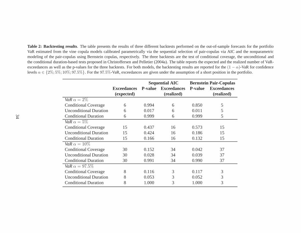
Table 2: Backtesting results. The table presents the results of three different backtests performed on the out-of-sample forecasts for the portfolioVaR estimated from the vine copula models calibrated parametrically via the sequential selection of pair-copulas via AIC and the nonparametricmodeling of the pair-copulas using Bernstein copulas, respectively. The three backtests are the test of conditional coverage, the unconditional andthe conditional duration-based tests proposed in Christoffersen and Pelletier (2004a). The table reports the expected and the realized number of VaR-exceedances as well as the p-values for the three backtests.For both models, the backtesting results are reported for the (1 − α)-VaR for confidencelevelsα ∈ {2%; 5%; 10%; 97.5%}. For the97.5%-VaR, exceedances are given under the assumption of a short position in the portfolio.
Sequential AIC Bernstein Pair-CopulasExceedances P-value Exceedances P-value Exceedances(expected) (realized) (realized)
VaRα = 2%Conditional Coverage 6 0.994 6 0.850 5Unconditional Duration 6 0.017 6 0.011 5Conditional Duration 6 0.999 6 0.999 5VaRα = 5%Conditional Coverage 15 0.437 16 0.573 15Unconditional Duration 15 0.424 16 0.186 15Conditional Duration 15 0.166 16 0.132 15VaRα = 10%Conditional Coverage 30 0.152 34 0.042 37Unconditional Duration 30 0.028 34 0.039 37Conditional Duration 30 0.991 34 0.990 37VaRα = 97.5%Conditional Coverage 8 0.116 3 0.117 3Unconditional Duration 8 0.053 3 0.052 3Conditional Duration 8 1.000 3 1.000 3
34