snake river spring/summer chinook … river spring/summer chinook salmon habitat feasibility study...

SNAKE RIVER SPRING/SUMMER CHINOOK SALMON HABITAT FEASIBILITY STUDY

ANNUAL PROGRESS REPORT 2001

Pete McHugh [email protected]

and

Phaedra Budy

[email protected]

Utah Cooperative Fish and Wildlife Research Unit Department of Fisheries and Wildlife

Utah State University Logan, UT 84322-5290

March 2002

CONTENTS

Page

ACKNOWLEDGEMENTS 3 PREFACE 4 LIST OF TABLES 5 LIST OF FIGURES 8

CHAPTER I: Executive summary, Introduction, and study stream descriptions

EXECUTIVE SUMMARY 14 INTRODUCTION 17 STUDY STREAM DESCRIPTIONS 19 TABLES 20 FIGURES 23 REFERENCES 27

CHAPTER II: A spawning and rearing habitat assessment for selected index streams in Oregon and Idaho

INTRODUCTION 29 METHODS 29 Survey design 30 Spawning gravel variables 30 Embeddedness 31 Pool variables and habitat composition 31 Discharge measurement 32 Temperature variable measurement 32 Spatial variability of spawning gravel quality 32

RESULTS 32 Spawning gravel variables 33 Core sampling in Elk Creek 33

Embeddedness 33 Pool variables and habitat composition 34 Discharge measurement 34 Temperature variables 34 Spatial variability of spawning gravel quality 35

CONCLUSIONS 35 RECOMMENDATIONS 36 TABLES 38 FIGURES 40 REFERENCES 53

McHugh & Budy 2002 1

CHAPTER III: An assessment of Snake River spring/summer chinook salmon spawning habitat selection and site suitability in Elk Creek, Idaho

INTRODUCTION 55 METHODS 56 Study site description 56 Survey design 56 Spawning habitat variable measurement 57 Assessing redd presence/absence 57 Statistical analyses 57

RESULTS 58 CONCLUSIONS 59 FUTURE ANALYSES 61 TABLES 62 FIGURES 64 REFERENCES 68

CHAPTER IV: Modeling early life-stage survival for selected Snake River spring/summer chinook salmon populations based on spawning and rearing habitat quality

INTRODUCTION 71 MODEL BACKGROUND 71

Early life history of chinook salmon 72 Habitat variables used in model 72

METHODS 73 Index stream approach 73 Model description 73 Input data description 74 Simulation approach 75 Model evaluation dataset 75

RESULTS 77 CONCLUSIONS 78 FUTURE DIRECTION 79 TABLES 81 FIGURES 83 APPENDICES 89

Model computations 89 Snorkel surveys 92

Tables 98 Figures 101

REFERENCES 102


ACKNOWLEDGEMENTS We would like to thank the U.S. Fish and Wildlife Service and the U.S. Geological Survey for funding this study. In addition, we would like to offer special thanks to Howard Schaller at the Columbia River Fisheries Program Office for initiating and supporting this study. We thank Gary Thiede and Brian Jacoby for their assistance, both in the field and at the Fish Ecology Lab, and Charlie Petrosky at the Idaho Department of Fish and Game for developmental and supervisory support. Finally, we would like to thank the many biologists at the U.S. Forest Service, Idaho Department of Fish and Game, and Oregon Department of Fish and Wildlife who provided us with valuable information that aided us in both project planning and implementation.


Preface This report has been written such that all information could be conveyed in an efficient manner. While the central theme of the report is salmon habitat quality assessment and improvement feasibility, the ideas and explicit objectives of the different sections are quite different and comprehensive. Thus, for the purposes of organization it was best to treat them as separate documents. To avoid repetition, however, some components (e.g., site maps) of one section may be referenced in others. The basic sequence of each chapter follows the format: 1) text body, 2) tables, 3) figures, 4) references, and 5) appendices. The chapters are:

Chapter I. Executive summary, introduction, and study stream descriptions

Chapter II. A spawning and rearing habitat assessment for selected index streams in Oregon and Idaho Chapter III. An assessment of Snake River spring/summer chinook salmon spawning habitat selection and site suitability in Elk Creek, Idaho Chapter IV. Modeling early life-stage survival for selected Snake River spring/summer chinook salmon populations based on spawning and rearing habitat quality


LIST OF TABLES

Table Page

Chapter I

1.1 Summary of index streams selected for field data collection and modeling efforts during 2001.

20

1.2 Habitat and water quality conditions for study streams. A period denotes that information for that field was unavailable.

21

1.3 Qualitative summary of land use activities existing within index watersheds under study. A period denotes that information for that field was unavailable.

22

Chapter II

2.1 List of variables measured during summer 2001 in index streams.

38

2.2 Sample size details for index streams. “km” is the number of river kilometers surveyed during sample period. Sample is total number of pools (P) and riffles (R) that were sampled during survey. Pebble count and embeddedness categories are the number of pool and riffles sampled in which those measurements were made. See text for further details.

38

2.3 Descriptive statistics from Elk Creek core samples. Percent fines are by weight. D50 computed from cumulative frequency distribution. Rkm = river kilometer, n = sample size (total number of sites for All sites row), SE = standard error.

39

2.4 Summary of habitat unit composition from habitat surveys of publicly owned reaches by index stream. Pool:Riffle ratio is by area.

39

2.5 Comparison of percent composition (by area) for pools and riffles, estimated from sampled units and for the entire population (“population” value is from census of all sites in index stream, not just sampled sites) for Elk and Sulphur creeks.

39


Chapter III

3.1 Values of D50, velocity, and depth for this and previous studies.

62

3.2 Descriptive statistics for sites with and without redds. n =number of sites, SE = standard error, and CV = coefficient of variation. D50 is in mm, depth is in m, and velocity is in m/s.

62

3.3 Results from logistic regression on Elk Creek redd P/A data.

62

3.4 Error rates for logistic regression model with all variables. Includes resubstitution and crossvalidation misclassification error rates for overall prediction (Total) and within classes (Predicted present and absent).

63

3.5 Results from stepwise logistic regression on Elk Creek redd P/A data.

63

3.6 Error rates for logistic regression model with all variables. Includes resubstitution and crossvalidation misclassification error rates for overall prediction (Total) and within classes (Predicted present and absent).

63

Chapter IV

4.1 Table of habitat variables modeled with details on which life stages are affected and the mechanism by which the effect is manifested.

81

4.2 Descriptive statistics for model predicted egg-to-parr survival rates by index stream from 1,000 Monte Carlo trials (n). Standard deviation (SD) is reported as n was identical for all index stocks.

81

4.3 Descriptive statistics for model predicted egg-to-smolt survival rates by index stream from 1,000 Monte Carlo trials (n). Standard deviation (SD) is reported as n was identical for all index stocks.

82

A.1 Strata characteristics for study streams.

98

A.2 Fish species encountered and level of detail recorded during observation.

98

A.3 Population estimates, upper and lower confidence bounds (UCB and LCB), and relative confidence intervals (CI) for selected species in Elk and Sulphur Creek for summer of 2001.

99


A.4 Egg-to-parr survival (S) estimates for Elk and Sulphur creeks for brood year 2000 and from past studies.

99

A.5 Mean (standard error) density of fish species encountered during summer 2001 snorkel surveys by habitat and stratum in study streams.

100


LIST OF FIGURES

Figure Page

Chapter I

1.1 Map of Upper Grande Ronde River study reach. Flow direction is from south to north. The reach used primarily for chinook spawning and rearing extends from just upstream of Meadow Creek to immediately upstream of the East Fork Grande Ronde River. Reaches downstream are used primarily for rearing and migration.

23

1.2 Map of Minam River study reach. Flow direction is from south to north. The reach used primarily for chinook spawning and rearing extends from just upstream of Murphy Creek to approximately 10 km upstream of the North Minam River. Some spawning also occurs in the Little Minam River. Reaches downstream are used primarily for rearing and migration.

24

1.3 Map of Elk Creek study reach. Flow direction is from northwest corner to southeast corner of map. The primary spawning and rearing reach extends from the confluence with Bear Valley Creek upstream to West Fork Elk Creek.

25

1.4 Map of Sulphur Creek study reach. Flow direction is from west to east. Spawning occurs primarily from upstream of the second nameless tributary entering from the south (heading upstream) to near Moonshine Creek, though some spawning and rearing does occur outside of this reach.

26

Chapter II

2.1 Map of Upper Grande Ronde River study reach showing sample (squares) and thermograph sites (circles). Flow direction is from south to north. The reach used primarily for chinook spawning and rearing extends from just upstream of Meadow Creek to immediately upstream of the E. F. Grande Ronde River. Reaches downstream are used primarily for rearing and migration.

40


2.2 Map of Minam River study reach showing sample (squares) and

thermograph sites (circles). Flow direction is from south to north. The reach used primarily for chinook spawning and rearing extends from just upstream of Murphy Creek to approximately 10 km upstream of the N. Minam River. Some spawning also occurs in the Little Minam River. Reaches downstream are used primarily for rearing and migration. Note that the lowermost thermograph is located outside of the main spawning and rearing reach.

41

2.3 Map of Elk Creek study reach showing sample (squares) and thermograph sites (circles). Flow direction is from northwest corner to southeast corner of map. The primary spawning and rearing reach extends from the confluence with Bear Valley Creek upstream to W. F. Elk Creek.

42

2.4 Map of Sulphur Creek study reach showing sample (squares) and thermograph sites (circles). Flow direction is from west to east. Spawning occurs primarily from upstream of the second nameless tributary entering from the south (heading upstream) to near Moonshine Creek, though some spawning and rearing does occur outside of this reach.

43

2.5 Box-and-whisker plots of spawning gravel variables calculated from all pebble counts for pool (a., b., and c.) and riffle (d., e., and f.) sites in each index stream. Box upper and lower boundaries correspond to quartiles. The thin line in the middle is the median, the bold line is the mean, and whiskers correspond to the 10th and 90th percentiles. All other box-and-whisker plots in this report have the same format. Small squares beyond whiskers are outliers.

44

2.6 Box-and-whisker plots of cobble embeddedness (%) for pool (a.) and riffle (b.) sites in each index stream. Box upper and lower boundaries correspond to quartiles. The thin line in the middle is the median, the bold line is the mean, and whiskers correspond to the 10th and 90th percentiles. Small squares beyond whiskers are outliers.

45

2.7 Relationship between visually estimated embeddedness rating (from Platts et al. 1983; where 1 = >75% embedded, 2 = 50 – 75% embedded, 3 = 25 – 50% embedded, 4 = 5 – 25% embedded, and 5 = < 5% embedded) for pool and riffle sites combined for all streams. Simple linear regression for riffle habitats produced the equation: Hoop = 66.2 – 9.5visual (r2 = 0.29, df = 1, F = 16.4, p = 0.0002). For pool habitats, the equation is: Hoop = 73.5 – 10.8visual (r2 = 0.44, df = 1, F = 50.3, p < 0.0001).

46


2.8 Mean pool area (a.), pool maximum depth (b.), percent pools (by area, c.) and mean wetted width (d.), for pools sampled in each index stream. Error bars correspond to one standard deviation.

47

2.9 Daily average temperature (oC) for the period of 9 July – 21 September 2001 for low, middle, and high temperature measurement sites in Idaho study streams. Average was computed from 18 daily measurements logged at 90-minute intervals.

48

2.10 Daily average temperature (oC) for the period of 9 July – 21 September 2001 for low, middle, and high temperature measurement sites in Oregon study streams. Averages were computed from 18 daily measurements logged at 90-minute intervals.

49

2.11 Daily average temperature and daily maximum temperature for the period of 9 July – 21 September 2001 averaged for all sites in each index stream. Average was computed from 18 daily measurements logged at 90-minute intervals at three sites (Sulphur Ck. = 2 sites) in each stream. Reference lines are for the temperature where growth is optimum (solid line, 14.8 oC) and where zero net growth begins (dotted line, 19.1 oC) for juvenile chinook salmon (reviewed in Armour 1991).

50

2.12 D50 (with 1 SE; a.) and percent fines (< 10 mm; b.) values from individual pool and riffle pebble counts in Elk Creek plotted against river kilometer. River kilometer = 0 is uppermost sample location, immediately downstream of West Fork Elk Creek confluence.

51

2.13 Map of Elk Creek with graduated symbols for D50 calculated from pebble counts at individual sample sites. Flow direction is from northwest corner to southeast corner.

52

Chapter III

3.1 Schematic representation of how the gravel size distribution, mean velocity, and mean depth measurements were made at each pool tail (the preferential spawning location for chinook salmon). A. Longitudinal cross-section of pool. B. Aerial view of pool-tail measurement area.

64


3.2 Box plots for D50, depth, and velocity for Elk Creek sample sites

with (n = 23) and without (n = 20) chinook salmon redds. Box upper and lower boundaries correspond to quartiles, the narrow mid-line is the median, the bold mid-line is the mean, and the whiskers are the 10th and 90th percentiles. Small squares beyond whiskers represent outliers.

65

3.3 Three-dimensional scatter plot of sampled sites with and without chinook salmon redds.

66

3.4 Longitudinal trend in gravel size in Elk Creek. Vertical line separates upper Elk Creek (upstream of Bearskin Creek) from lower Elk Creek. Circled sites are sites in lower Elk Creek where chinook spawned. River kilometer 0 corresponds to the top of the study reach (West Fork Elk Creek confluence).

67

Chapter IV

4.1 Sequence of life stages and events occurring during egg-to-smolt stages of Snake River spring/summer chinook salmon life history. The points in the life cycle that modeled habitat parameters affect survival is indicated by connecting arrows. Specific mechanisms causing potential survival reductions are reviewed in Table 4.1.

83

4.2 Graphical illustration of survival-habitat variable functions used in computing egg-to-parr (a-d) and egg-to-smolt survival (a-e). a. is logarithmic function from Stowell et al. 1983 based on work of Tappel and Bjornn 1984; b. is a second degree polynomial function based on data points in Murray and McPhail 1988 and Armour 1991; c. is a second degree polynomial function from Stowell et al. 1983, based on work of Bjornn et al. 1977; d. is a Weibull function based on a combination of data points from Brett 1952, Coutant 1973, McCormick et al. 1972; e. is logarithmic function from Stowell et al. 1983 based on work of Bjornn et al. 1977.

84

4.3 An example of a cumulative frequency curve used in Monte Carlo trials. Data represented are from Elk Creek percent fines values measured at 43 potential spawning sites. The simulated distribution was obtained from 1,000 samples drawn from the empirical distribution.

85

4.4 Plot of mean egg-to-smolt survival by number of Monte Carlo trials for Elk Creek index area. The standard deviation of the mean stabilized to 4% at approximately n = 350 trials.

86


4.5 Distributions of model predicted egg-to-parr and egg-to-smolt survival based on 1,000 Monte Carlo trials for each index stream. Box upper and lower boundaries correspond to quartiles. The thin line in the middle is the median, the bold line is the mean, and whiskers correspond to the 10th and 90th percentiles.

87

4.6 Plot of observed vs. predicted egg-to-parr and egg-to-smolt survival rates. The slope of a line between egg-to-parr points is 1.11 (intercept = 25.2) , while the slope between the two egg-to-smolt points is 1.00 (intercept = - 3.7). As there were only two points in both egg-to-parr and egg-to-smolt cases, formal regression hypothesis tests (i.e., F statistic could not be computed) were not conducted.

88

A.1 Mean fish density in pool habitats (combined strata) in Elk and Sulphur Creeks, summer 2001. Error bars correspond to one standard error.


CHAPTER I

EXECUTIVE SUMMARY, INTRODUCTION, AND STUDY STREAM DESCRIPTIONS


EXECUTIVE SUMMARY

Introduction Recent modeling efforts by the National Marine Fisheries Service (NMFS) suggest that recovery of Snake River spring/summer chinook salmon (Oncorhynchus tshawytscha) is possible with modest improvements in estuary and freshwater spawning and rearing habitat (Kareiva et al. 2000). Consequently the most recent Biological Opinion on the operation of the hydrosystem places considerable emphasis on improving freshwater spawning and rearing habitat conditions, in lieu of dam breach. While most biologists would agree that improvements in freshwater spawning and rearing habitat quality have directly benefited chinook salmon, there is considerable disagreement as to whether this approach alone will facilitate recovery of the evolutionarily significant unit (ESU) as a whole. Stocks spawning in “pristine” habitats, like those in the headwaters of Idaho’s Middle Fork Salmon River, have declined similarly to those in highly degraded habitats. These observations suggest that freshwater spawning and rearing habitat improvement may substantially change first year survival for those stocks in degraded spawning and rearing habitat, but for many stocks, improving habitat quality is unlikely to lead to population recovery. Our primary objective is to evaluate the potential for improving survival through the early freshwater life stages via habitat improvements. Due to the precarious nature of chinook salmon stock persistence, it is important that a field-based, quantitative assessment be made. Within this framework, the short-term (5-10 years) feasibility of habitat improvements must also be considered, given the high risk of extinction faced by these stocks. Our approach for meeting this objective was as follows: 1) collect baseline habitat and fish population data for selected populations of chinook salmon (either from original field surveys, or from existing documents and datasets), 2) develop a habitat-based life cycle model that uses data from Step 1 for inputs and model calibration, to predict egg-to-parr and egg-to-smolt survival, and 3) simulate the survival response to habitat improvement scenarios using the habitat-based life cycle model. In addition to these steps, we have also investigated questions of spawning habitat selection/suitability for chinook salmon.

Habitat Assessments

Our habitat assessments generally corroborate published qualitative rankings on habitat quality in the Upper Grande Ronde and Minam rivers and Elk and Sulphur creeks. Sulphur Creek and the Minam River are reported to be in good condition, while the Upper Grande Ronde River is considered fair, and Elk Creek is considered poor. We rate these four streams similarly, with the exception of the Upper Grande Ronde River, which we believe to contain poor quality habitat, and Elk Creek, which we rate fair to good. The Upper Grande Ronde River, the study steam with the most extensive management history, contained the worst


habitat conditions of the four streams under study (relatively high percent fines and embeddedness levels, potential for summer temperature to be limiting). Conversely, the Minam River and Sulphur Creek, two wilderness streams, contained good spawning and rearing habitat conditions (e.g., relatively low embeddedness and fine sediment levels). Sulphur Creek and Elk Creek were quite similar with respect to embeddedness, percent fines, and temperature variables; however, they deviated substantially in habitat unit composition.

Spawning Site Selection

In addition to our habitat assessments and modeling, we were also interested in increasing our understanding of what type of habitat constitutes suitable spawning habitat for a single population of Snake River spring/summer chinook salmon (Elk Creek index stock) through the use of logistic regression methods. We developed a logistic regression model relating redd presence or absence to spawning habitat characteristics using a dataset consisting of habitat variable measurements taken at potential spawning sites (pool tails - without any a priori knowledge of where spawning had occurred in the past) during the summer of 2001 coupled with a post-spawning determination of redd presence or absence. Our findings suggest that chinook spawning site suitability in Elk Creek is strongly affected by the coarseness of the gravel (as measured by D50, the median gravel diameter), secondarily by water depth, and less so by water velocity. Salmon chose spawning sites with coarser gravel, a higher water velocity, and a shallower depth, when compared to sites that were not used for spawning.

Habitat Assessment and Freshwater Survival Modeling Our model appeared to reasonably capture the effects of habitat and the range of conditions observed across the index areas we modeled. Model predictions of egg-to-smolt survival were lower in the Upper Grande Ronde River than in the Minam River in Oregon. Predictions of egg-to-parr survival were higher in Sulphur Creek relative to Elk Creek in Idaho. When comparing across the four index stocks, mean predicted egg-to-smolt survival ranged from a high of 10.0 % in Sulphur Creek, to a low of 3.5 % in the Upper Grande Ronde River. The general ranking in predicted egg-to-smolt survival (in increasing order) across stocks is therefore: Upper Grande Ronde < Elk < Minam < Sulphur. The trend in model predictions of freshwater survival closely agree with the general pattern of habitat quality experienced by these four stocks. The Upper Grande Ronde River is considered to contain moderate to poor quality habitat, while the Minam River and Sulphur Creek are both considered to be in near pristine condition. As with the egg-to-smolt survival prediction, Elk Creek habitat quality is intermediate of these extremes. Taken together, these observations suggest that of the four stocks in question, the Upper Grande Ronde stock has the greatest potential for experiencing a survival benefit from habitat


improvements. Second to this is Elk Creek, which may experience a minor survival benefit from habitat improvements (primarily in the lower reaches). As opportunities for improving habitat conditions in the Minam River and Sulphur Creek are negligible, the potential for improving early life stage survival for these stocks is extremely limited. As expected, our model predictions diverged from observed survival estimates due to the purposeful omission of biotic components that affect egg-to-smolt survival (e.g., predation). We incorporated only a subset of physical habitat variables that are both directly linked to survival and targeted for improvement. A consistent bias in predictions, however, suggests that the habitat variables and survival functions selected account for a consistent amount of survival in our study streams. Future model calibration will account for unexplained biotic mortality and allow for more direct comparisons between predicted survival and observed survival. At this stage, however, our model predictions serve as a useful index of habitat-related early life stage survival that allows us to compare the potential for improving habitat across index areas. The next phase of our modeling exercise will include a model calibration aimed at accounting for unexplained biotic mortality and any bias in our predictions. Our model will be calibrated to predict “true” egg-to-smolt and egg-to-parr survival rates instead of the current index of physically-affected survival. Calibration will be followed by the forecasting of feasible habitat improvement scenarios for each stock with explicit consideration of the Reasonable and Prudent Alternative habitat actions identified in the Biological Opinion. Ultimately our model predictions of freshwater survival will be evaluated within the context of the entire chinook salmon life cycle using an abbreviated PATH life cycle model, in coordination with the U.S. Fish and Wildlife Service’s Columbia River Fisheries Program Office (CRFPO). These analyses will allow us to determine whether habitat improvement-related survival benefits are sufficient to offset mortality costs incurred in other life stages and decrease the risk of extinction of the ESU overall. In addition, we will be including habitat assessment and population analyses for two new index streams in 2002 (possibly Lemhi and Pahsimeroi) and revisiting several of last years streams to gain additional survival information and fill in any habitat assessment gaps.


Introduction Snake River spring/summer chinook salmon, Oncorhynchus tshawytscha, (hereafter referred to as chinook salmon) were listed as a threatened species under the Endangered Species Act in 1992, due to precipitous declines in run sizes throughout the 20th century (NMFS 1992). Habitat degradation, hydropower development, hatchery practices, and harvest are identified as causal agents in this decline. Recent modeling efforts by the National Marine Fisheries Service (NMFS) suggest that recovery of these fish is possible with modest improvements in estuary and freshwater spawning and rearing habitat (Kareiva et al. 2000). Therefore, there has been a recent emphasis on improving freshwater spawning and rearing habitat conditions. While most biologists would agree that improvements in freshwater spawning and rearing habitat quality have directly benefited chinook salmon, there is considerable disagreement as to whether this approach alone will facilitate recovery of the evolutionarily significant unit (ESU) as a whole. For example, based on smolt to spawner ratios, Petrosky et al. (2001) determined that the decline of chinook salmon since the 1960s was of a magnitude too great to be attributed to reduced freshwater spawning and rearing habitat quality alone. In addition, stocks spawning in “pristine” habitat, like those in the headwaters of Idaho’s Middle Fork Salmon River, have declined similarly to those in highly degraded habitat. These observations suggest that for some stocks, improving habitat quality is unlikely to lead to population recovery; however, freshwater spawning and rearing habitat improvement may substantially change first year survival for those stocks in degraded spawning and rearing habitat. As a primary component of the chinook salmon recovery strategy, the potential for improving survival through the early freshwater life stages via habitat improvements needs to be evaluated. Due to the precarious nature of chinook salmon stock persistence, it is important that a field-based, quantitative assessment be made. Within this framework, the short-term (5-10 years) feasibility of habitat improvements must also be considered, given the high risk of extinction faced by these stocks. It is the objective of this research to address these concerns through the following steps:

1. The collection of baseline habitat and fish population data for selected

populations of chinook salmon (either from original field surveys, or from existing documents and datasets)

2. The development of a habitat-based life cycle model that uses data from step 1 for inputs and model calibration, to predict egg-to-parr and egg-to-smolt survival

3. The simulation of the survival response to habitat improvement scenarios using the habitat-based life cycle model.


In addition to these steps, we have also investigated questions of spawning habitat selection and suitability for chinook salmon. The following report contains our detailed findings for year one of a two-year study.


Study site description

Snake River spring/summer chinook salmon populations are distributed over a large area (nearly 250,000 km2) characterized by a great diversity of geologic, climatic, habitat, and management conditions. To best capture this diversity, we selected a subset of index stocks for both field sampling and modeling efforts. Snake River chinook index stocks are associated with long term data (nearly 50 years in most cases) on population trends, primarily in the form of annual redd counts, and have been used in past modeling assessments of the ESU (e.g., CRI, Kareiva et al. 2000; PATH, Peters and Marmorek 2001). We selected our subset based on current habitat conditions and the availability of fish population data, such that the range of habitat conditions (i.e., from degraded to “pristine”) found in the Snake River Basin is represented (Table 1.1). During the summer of 2001, we conducted habitat surveys in two Oregon streams, the Upper Grande Ronde and Minam rivers, and two Idaho streams, Elk and Sulphur creeks (Figures 1.1 – 1.4). In addition, we performed snorkel surveys in both Idaho streams and obtained fish population data from the Oregon Department of Fish and Wildlife (ODFW) for the Minam and Grande Ronde rivers. The Minam River and Sulphur Creek are considered high quality spawning and rearing streams, while Elk Creek is considered moderate quality, and the Upper Grande Ronde is considered fair to poor quality. For a more detailed description of the habitat conditions, land uses, and other relevant details see Tables 1.2 – 1.3.


Table 1.1. Summary of index streams selected for field data collection and modeling efforts during 2001.

Stream Ecoregiona Dominant Geology

Management Status Ownership

Habitat Conditionsb Fish Population Data

Upper Grande Ronde River

Blue Mountain Mixed Managed Mixed Fair annual redd counts, smolt trapping

Minam River Blue Mountain Mixed Wilderness Federal Good annual redd counts, smolt trapping

Elk Creek Northern Rockies Granitic Managed Federal Poorc annual redd counts, parr density monitoring, few parr population estimates

Sulphur Creek Northern Rockies Granitic Wilderness Federal Good annual redd counts, parr density monitoring, few parr population estimates

a. Omernik (1987) ecoregions. b. From Beamesderfer et al. (1997) c. Bear Valley/Elk combined index stock is considered poor, though Elk Creek tends towards having fair to good conditions.


Table 1.2. Habitat and water quality conditions for study streams. A period denotes that information for that field was unavailable.

Habitat Quality Rating a Percent of stream length with rating b sec. 303(d) listings d Stream S/R DR OW Excellent Good Fair Poor c Sed. Temp. otherU. Grande Ronde R. . . . 0 17 34 49 Ye Ye n,h,f,dMinam R. 1 Y

1 1 17 20 47 16 Yf f NoneBear Valley/Elk Ck.g

3 2 1 17 61 22 0 Yg N None

Sulphur Ck. 1 1 1 43 19 38 0 N N None

a. From Marmorek (1996). S/R = spawning and rearing; DR = downstream rearing; and OW = overwinter; 1 = high, 2 = intermediate, and 3 = low. These ratings were a result of a qualitative assessment performed by state agencies used primarily for ranking purposes and PATH modeling.

b. Data from NWPPC 1990/1991 subbasin planning, from Streamnet (http://www.streamnet.org). Habitat ratings (Excellent, Good, Fair, and Poor) were assigned to reaches defined by three categories of chinook salmon use: migration, spawning and rearing, and rearing and migration. Reaches represented are only those defined as spawning and rearing, and rearing and migration, since reaches used primarily as migration corridors were not rated. Not all stream reaches were included in survey. All habitat ratings were assigned by professionals with local expertise on the given stream or watershed. Stream lengths included in calculation were all main stem reaches and tributaries upstream from (and including) PATH index areas.

c. Most reaches on Grande Ronde R. downstream from PATH index areas (defined use: rearing and migration) were rated poor to fair. d. Parameters for which the stream, or a given reach is identified as water quality limited under section 303(d) of the Clean Water Act. Only those

that most affect fish or those affecting fish in their migrations are listed. Y = yes and N = no; n=excessive nutrients, h=habitat modification, f=flow alteration, and d=dissolved oxygen. Sources: EPA's Surf Your Watershed, and ODEQ (2000).

e. Principal land uses responsible for water quality problems in the upper Grande Ronde are: forest disturbances (both within and outside of riparian areas), agricultural riparian and upland disturbances, road construction, and urban/suburban development (ODEQ 2000). Substantial pool loss has occurred in the upper Grande Ronde River as a result of sedimentation (McIntosh et al. 1994a, 1994b). The quality of habitats for chinook salmon has been severely reduced (affecting survival at many life stages) due to increased temperature, increased sedimentation, changes in flow, riparian alteration, and bank destabilization (Mobrand and Lestelle 1997). Most of the 303(d) listings in the "other" category occur below PATH index areas, but likely affect the stock.

f. Reach listed is below main spawning reach, within segment designated by ODFW as used primarily for rearing and migration. Management occurred within the Minam River historically, however it is considered to be near “pristine” today.

g. Data are for aggregated Bear Valley/Elk stock. Sedimentation has led to pool loss and degradation of spawning and rearing habitats in Bear Valley (Beamesderfer et al. 1997). Poor egg-to-parr survival or early downstream migration of juvenile chinook is a potential consequence of excessive fine sediments in Bear Valley (Scully and Petrosky 1991).


Table 1.3. Qualitative summary of land use activities existing within index watersheds under study. A period denotes that information for that field was unavailable.

Land Use Activities Stream Logging Mining Roads Irrigation Grazing OtherUpper Grande Ronde R.a Y Y Y Y Y urbanizationMinam R.b Y

N N N Y . Bear Valley/Elk c

Y Y Y N Y .

Sulphur C. d N N N N N . a. Timber harvest in the upper Grande Ronde River watershed has occurred since the late 1800s and has been steadily increasing since the 1950s (McIntosh et

al. 1994a; McIntosh et al. 1994b), though harvest has slowed substantially in the 1990s (Wallowa-Whitman National Forest 1999). Splash dams were often used to transport timber via waterways, and have been noted as a habitat-degrading remnant of historical timber harvest activities (McIntosh et al. 1994a; McIntosh et al. 1994b). Also, railroads constructed for transporting timber out of the uplands have constrained reaches of the Grande Ronde River (Wallowa-Whitman National Forest 1999). Mining activities in the watershed have contributed to degraded chinook habitat conditions as well. Tailings piles, many of which are located near important chinook spawning areas, have constrained the channel in some areas and serve as chronic sources of sediment (affecting nearly 5 km of stream; McIntosh et al. 1994a; McIntosh et al. 1994b; Wallowa-Whitman National Forest 1999). Sections of these mining sites are designated as historical monuments and cannot be actively restored as a result. Road density in the index portion of the watershed is moderate. Irrigation diversions do not exist in the index reach of the upper Grande Ronde, though there are numerous diversions downstream. Portions of this watershed were severely overgrazed as early as the 1880s but conditions have since improved substantially. Grazing continues to occur, though riparian fences exist in some areas and a variety of rotation schemes are being employed to minimize negative impact (Wallowa-Whitman National Forest 1999). The primary section of the river that is affected by grazing occurs on private land. Urbanization is substantial downstream of the index reach in the city of La Grande, Oregon.

b. The Minam River is currently unmanaged, however, substantial timber harvest occurred within the drainage historically (early 1900s). A small, private outfitter lodge and multiple airstrips currently exist in the drainage.

c. Information pertains to aggregated Bear Valley/Elk index stock. Timber harvest in Bear Valley Creek is limited to post-and-pole sales (Beamesderfer et al. 1997). The Bear Valley Mine produced tailings piles that have contributed substantial volumes of sediment to the creek. Active restoration projects sponsored by the Shoshone-Bannock Tribe to deal with mine related sediment problems have been implemented (Beamesderfer et al. 1997). The drainage historically contained roads and still does. Grazing is believed to be the most degrading land use activity occurring in the Bear Valley Creek watershed. A Bureau of Fisheries survey of Bear Valley Creek reported that livestock were a problem as early as 1941 (McIntosh et al. 1995). Grazing rights in the Elk Creek Allotment were recently (2000) purchased by the Bonneville Power Administration (BPA) as part of the Fish and Wildlife Program (Boise National Forest 2000). Grazing continues in the Deer Creek and Bear Valley Creek Allotments. Sulphur Creek is perhaps in the best condition of all of the proposed streams, as it is the least managed of all watersheds, both historically and today. Timber harvest and road construction have not occurred in the watershed historically (Beamesderfer et al. 1997). Grazing in the Sulphur Creek watershed is limited to a small fenced horse pasture and any "slop-over" grazing from other allotments (which IDFG personnel believe is limited). In addition, one small outfitter ranch exists in the watershed, which has negligible impact. Bureau of Fisheries personnel surveying the area in 1941 noted that "all in all this is one of the best salmon stream tributaries to the Middle Fork and although relatively small in size, it can care for several thousand spawning salmon and should be protected and kept open…" (McIntosh et al. 1995).


N

0 5 10 15 20 25 30 Kilometers

Beaver Creek

Approximate location ofprivate property

Grande Ronde River

#

Meadow Creek

Grande Ronde River

#

Fly Creek

Sheep Creek E. F. Grande Ronde River

Figure 1.1. Map of Upper Grande Ronde River study reach. Flow direction is from south to north. The reach used primarily for chinook spawning and rearing extends from just upstream of Meadow Creek to immediately upstream of the East Fork Grande Ronde River. Reaches downstream are used primarily for rearing and migration.


N

Oregon

0 5 10 15 20 25 Kilometers

Trout Creek

Murphy Creek

Minam River

Little Minam River

#

N. Minam River

Figure 1.2. Map of Minam River study reach. Flow direction is from south to north. The reach used primarily for chinook spawning and rearing extends from just upstream of Murphy Creek to approximately 10 km upstream of the North Minam River. Some spawning also occurs in the Little Minam River. Reaches downstream are used primarily for rearing and migration.


W. Fork Elk Creek

Elk Creek

Bearskin Creek

Bear Valley Creek

0 1 2 3 4 5 Kilometers

N

Figure 1.3. Map of Elk Creek study reach. Flow direction is from northwest corner to southeast corner of map. The primary spawning and rearing reach extends from the confluence with Bear Valley Creek upstream to West Fork Elk Creek.


N


Middle ForkSalmon River

Sulphur Creek

Blue MoonCreek

Moonshine Creek

Full Moon Creek

Sulphur Creek

Figure 1.4. Map of Sulphur Creek study reach. Flow direction is from west to east. Spawning occurs primarily from upstream of the second nameless tributary entering from the south (heading upstream) to near Moonshine Creek, though some spawning and rearing does occur outside of this reach.


References Beamesderfer, R. C. P., H. A. Schaller, M. P. Zimmerman, C. E. Petrosky, O. P. Langness, and

L. LaVoy. 1997. Spawner-recruit data for spring and summer chinook salmon populations in Idaho, Oregon, and Washington. Draft report to: Marmorek, D. R., and C. N. Peters (eds.). J. Anderson, R. Beamesderfer, L. Botsford, J. Collie, B. Dennis, R. Deriso, C. Ebbesmeyer, T. Fisher, R. Hinrichsen, M. Jones, O. Langness, L. LaVoy, G. Matthews, C. Paulsen, C. Petrosky, S. Saila, H. Schaller, C. Toole, C. Walters, E. Weber, P. Wilson, M. P. Zimmerman. 1998. Plan for Analyzing and Testing Hypotheses (PATH): Retrospective and Prospective Analyses of Spring/Summer Chinook Reviewed in FY 1997. Compiled and edited by ESSA Technologies Ltd., Vancouver, B. C.

Boise National Forest. 2000. Final Bear Valley watershed analysis. 266 pp. plus appendices. Kareiva, P., M. Marvier, and M. McClure. 2000. Recovery and management options for

spring/summer chinook salmon in the Columbia River Basin. Science 290:977-979. Marmorek, D.R. (ed.), and 21 others. 1996. Plan for Analyzing and Testing Hypotheses (PATH):

Final report on retrospective analyses for fiscal year 1996. ESSA Technologies Ltd., Vancouver, B.C., Canada.

McIntosh, B. A., J. R. Sedell, J. E. Smith, R. C. Wissmar, S. E. Clarke, G. H. Reeves, and L. A. Brown. 1994a. Management history of eastside ecosystems; changes in fish habitat over 50 years, 1935 to 1992. Gen. Tech. Rep. PNW-GTR-321. Portland, OR: U.S. Dept. of Agriculture, Forest Service, Pacific Northwest Research Station. 55 p.

McIntosh, B. A., J. R. Sedell, J. E. Smith, R. C. Wissmar, S. E. Clarke, G. H. Reeves, and L. A. Brown. 1994b. Historical changes in fish habitat for selected river basins of Eastern Oregon and Washington. Northwest Science 68:36-53.

McIntosh, B.A., S.E. Clarke, and J.R. Sedell. 1995. Summary report for Bureau of Fisheries stream habitat surveys: Clearwater, Salmon, Weiser, and Payette River Basins 1934-1942. BPA project No. 89-104; DOE/BP-02246-2. Bonneville Power Administration, Portland, Oregon.

Mobrand, L and L. Lestelle. 1997. Application of the Ecosystem Diagnosis and Treatment method to the Grande Ronde Model Watershed Project. DOE/BP-61148-1. Bonneville Power Administration, Portland, Oregon.

NMFS (National Marine Fisheries Service). 1992. Endangered and threatened species; threatened status for Snake River spring/summer chinook salmon, threatened status for Snake River fall chinook salmon. Federal Register [Docket No. 910647-2043, 22 April 1992] 57(78):14,653-14,662.

Omernik, J. M. 1987. Ecoregions of the conterminous United States. Annals of the Association of American Geographers 77(1):118-125.

ODEQ (Oregon Department of Environmental Quality). 2000. Upper Grande Ronde Sub-basin total maximum daily load (TMDL) plan. State of Oregon Department of Environmental Quality, Portland, Oregon.

Peters, C.N., D.R. Marmorek. 2001. Application of decision analysis to evaluate recovery actions for threatened Snake River spring and summer chinook salmon (Oncorhynchus tshawytscha). Canadian Journal of Fisheries and Aquatic Sciences 58:2431-2446.

Petrosky, C.E., H.A. Schaller, and P. Budy. 2001. Productivity and survivial rate trends in the freshwater spawning and rearing stage of Snake River chinook salmon (Oncorhynchus tshawytscha). Canadian Journal of Fisheries and Aquatic Sciences 6:1196-1207.

Scully, R.J., and C.E. Petrosky. 1991. Idaho habitat/natural production monitoring. Idaho habitat evaluation for off-site mitigation record. Annual report, fiscal year 1989. Idaho Department of Fish and Game annual report to U.S. Department of Energy-Bonneville Power Administration, Portland, Oregon.

Wallowa-Whitman National Forest. 1999. Upper Grande Ronde Assessment Area Biological Assessment. 273 pp.


CHAPTER II

A SPAWNING AND REARING HABITAT ASSESSMENT FOR SELECTED INDEX STREAMS IN OREGON AND IDAHO


Introduction

The current strategy for chinook salmon recovery relies heavily on habitat improvements, both in freshwater spawning and rearing habitat and in the estuary and early marine environment. Therefore, there is a need for a compilation of information on current habitat conditions across the range of this ESU of Pacific salmon. This information is essential for an effective restoration strategy, as it could enable land managers and recovery specialists to target streams and stocks that would experience the greatest benefit from habitat restoration and improvement efforts. Due to differing habitat survey protocols being used by fisheries and land management agencies within the Snake River Basin (hereafter referred to as Basin) and the complete lack of data for some parameters, however, such information is only comparable at a coarse level of detail. Our primary objective is to generate a standardized dataset on habitat conditions in the Basin for use in our model-based assessment of survival improvement potential for selected salmon populations (Chapter IV). To fulfill this objective we performed a detailed habitat survey of a subset of Snake River spring/summer chinook salmon spawning and rearing index streams. In addition to fulfilling our modeling needs, data collected in our surveys provided a useful opportunity to address questions regarding sampling design and the spatial variability and longitudinal patterns for selected habitat parameters. The following is a concise summary of our findings on these matters.

Methods We surveyed all publicly owned reaches of the Upper Grande Ronde (UGR), Elk (ELK), and Sulphur (SUL) traditional redd count index areas during the summer of 2001. In the Minam (MIN) index reach, we surveyed a central ~ 7 km section that is considered to be the primary use area for Minam River chinook salmon (J. Zakel, ODFW, personal communication). Detailed maps of study reaches appear in Figures 2.1 – 2.4. Prior to field sampling, technicians received formal habitat survey training from U.S. Forest Service personnel working on the Interior Columbia Basin Effectiveness Monitoring Project. This multi-day training session emphasized objective, repeatable measurement of multiple habitat variables (for details on protocol see Henderson et al., in review). For our purposes, however, we measured a subset of these, as we were primarily interested in those variables (e.g., percent fines) that have been directly linked to survival and/or productive capacity for early salmon life stages in a given stream. A list of variables measured and reported here appears in Table 2.1.


Survey Design Habitat surveys were conducted within the framework of a ten percent (with the exception of the Minam River) systematic sample design based on channel units (pools and riffles, according to definitions of Henderson et al., in review). Pools were defined as concave, slow water units bounded by a head and tail crest. In order to be surveyed, pools had to occupy at least half of the wetted channel width, be at least as long as the wetted width, and have a maximum depth at least 1.5 times as deep as the tail crest depth. All channel units not meeting these criteria were placed in our riffle/run category. Channel units were limited to only two classes because increased complexity in habitat classification schemes can result in increased error (Roper and Scarnecchia 1995). A random starting point (between 1 and 10, for pools and riffles) was selected, and surveyors proceeded in an upstream direction numbering each pool or riffle. With the exception of temperature variables, habitat measurements were made in every tenth pool or riffle from the starting point. Spawning gravel variables Wolman pebble counts (Wolman 1954; Kondolf 1997) were conducted at each sampled pool tail and riffle where gravel (10-200 mm) predominated, as these were considered “potential” spawning sites. At each site, the b-axis of approximately 100 particles was measured to the nearest millimeter with a hand ruler. Particles with an intermediate axis less than 4 mm were recorded as < 4 mm. Pebble counts were not conducted if 50% or more of the pool tail or riffle was vegetated or consisted of silt and sand. From pebble counts at each site surveyed, the median gravel diameter (D50) and percent fines (< 7 mm, and < 10 mm; see note in Table 2.1 with justification for sizes reported) were calculated. While pebble counts were the most practical way to assess spawning gravel quality in our remote sites, they provide information only on the surficial size composition (Kondolf 2000). The subsurface gravel size composition, however, is a better approximation of conditions experienced by incubating salmon eggs, and can be quite different from surface conditions. Therefore, in addition to pebble counts, we collected bulk gravel core samples at six systematically spaced sites in lower Elk Creek on a pilot-study basis. At each site, three cores were taken using a McNeil-type corer (30 cm diameter tube; 25 cm average depth of core). Particles were sieved (through 64 and 16 mm sieves sizes), separated into size classes, and wet-weighed in the field; a subsample of the finer portion (< 16 mm) was retained for processing at the U.S. Forest Service’s Forestry Sciences Laboratory in Logan, Utah. After air-drying for several days, fines were passed through 8, 4, 2, and 1 mm sieves, and the constituents of each size class were weighed. The percent of the total sample < 8 mm and < 1 mm (by weight), and the D50 (from cumulative frequency distribution) are reported here.


Embeddedness The coarse component of the streambed is vital for summer rearing and overwintering of chinook salmon parr, and loss of interstitial spaces due to high sediment loads can severely reduce the productive capacity for riffle and pool habitats (e.g., Bjornn et al. 1977). We evaluated impairment for this habitat component in index streams using a modification of the Hoop Method (Skille and King 1989; MacDonald et al. 1991). Under our protocol, one 60 cm hoop was randomly located within each channel unit where particles > 75 mm were present (lower limit of substrate size identified as being utilized by juvenile chinook for overwintering; Bjornn and Reiser 1991). Within each hoop, the embedded height (De, the vertical height of the particle embedded in the sand matrix) and total vertical height (Dt) of each particle (> 75 mm) were measured after removing particle from the matrix while retaining its original spatial orientation. The embeddedness value for each hoop was then computed as the sum of all De’s divided by the sum of Dt’s, but it was also weighted if >10% of the hoop area was occupied by fines. In addition to measuring embeddedness with the hoop method, visual estimates of embeddedness (based on Platts et al. 1983) were made for use in evaluating visual methods for future sampling. Pool variables and habitat composition The maximum depth of sampled pools was measured by probing with a stadia rod. In situations where pool depth precluded safe measurement for this variable (deeper than wader height), the value was noted as > 2 m (10 times, primarily in Minam River). The length and width (average of a minimum of 4 systematically-spaced width measurements) of each sampled channel unit were measured using a metered tape so that unit area could be computed. From this we computed the percent of total surveyed area that was pool and riffle, as well as a pool to riffle area ratio. In addition to estimating the values for these parameters from our sample, we used data collected using the Basinwide Visual Estimation Technique (BVET; Hankin and Reeves 1988; Dolloff et al. 1993) in Elk and Sulphur creeks to compute the same parameters for the entire population. This habitat area estimation technique involves obtaining a visual estimate of area (product of estimated length and width) for all sites, including those between sampled sites, as well as accurately measuring the area of sampled sites. Using the accurately measured and visually estimated values for sampled sites, one can generate a correction factor for those sites where area was only visually estimated, yielding a “true” total area of pool and riffle for the entire stream. Values for these parameters obtained from the BVET were compared to those from the sample alone to determine if any sampling biases exist for these variables.


Discharge measurement Discharge was measured at one sampled riffle site each day using a Marsh-McBirney ® Flowmate 2000 electromagnetic flowmeter using standard methodology (Bain and Stevenson 1999). Data reported herein are averages of all measurements taken over the sampling period at an index stream, and are intended mainly for comparative purposes. In addition, discharge was measured at the Upper Grande Ronde and Minam rivers in the early fall to provide insight into the potential for temporal biases in flow-related variables (e.g., pool maximum depth). Temperature variable measurement Temperature loggers were used for collecting continuous data on stream temperature. In each index stream, Onset ® Optic Stowaway temperature loggers (accuracy ± 0.2 oC) were secured to the streambed in a well mixed, shaded location using rebar and cable (Figures 2.1 – 2.4). At minimum, two loggers were placed in each index stream, such that they were systematically spaced along the length of the stream. All loggers were set to record temperature at an interval of 90 minutes and were left in each stream from early July through the end of September. A logger central to each index reach was left through the winter season to gather information on egg incubation temperature conditions. From these data, a number of temperature metrics were calculated (Table 2.1). Spatial variability of spawning gravel quality In addition to comparing values for habitat parameters between the index streams, we also evaluated the spatial variability for selected parameters within a single stream (Elk Creek). Such an assessment can provide insight into sample design questions (i.e., if one cannot sample the entire index stream, where should samples be taken?) as well as the basic understanding of geomorphological processes (e.g., downstream fining). This assessment was made from a visual inspection of plots of selected spawning gravel variables against river kilometer.

Results During the period from 1 June through 5 August 2001, we surveyed a total of 70 kilometers of stream in four index areas, taking measurements on 87 pools and 52 riffles (Table 2.2). In Oregon, the Upper Grande Ronde River was characterized by higher embeddedness and percent fines levels, and warmer stream temperatures while the Minam River had lower values for these same variables. In Idaho, Elk and Sulphur creeks were similar with respect to all variables, with the exception of channel unit composition. Differences in values


for measured habitat variables were observed when all streams were compared. There was, however, considerable overlap in these distributions. Spawning gravel variables Results from pool-tail and riffle pebble counts indicate that the Upper Grande Ronde and Minam river index areas contain coarser gravels (a larger D50) than those of Elk and Sulphur creeks (Figures 2.5a, and 2.5d). The Elk Creek index area contained the finest gravels of all spawning areas surveyed (D50 mean for all Elk sites, 29 mm). The Upper Grande Ronde River and Elk Creek had higher mean levels of fine sediment (< 7 mm and < 10 mm) than did both Sulphur Creek and the Minam River, though the distributions for these variables overlapped between all streams (Figure 2.5). The general trend in spawning gravel variables between streams was similar for pool-tails and riffles. Core sampling in Elk Creek In addition to performing multiple pebble counts in Elk Creek, approximately 150 kilograms (total from 3 samples) of gravel were sampled at each of six sites using a McNeil core sampler. Percent fines < 1 mm (size class affecting incubation survival; Kondolf 2000) for all sites ranged from 4 – 13% (mean = 8%, SE = 3.2%; Table 2.3). Percent fines < 8 mm (approximately the size class affecting emergence success, < 10 mm; Kondolf 2000) ranged from 23 – 40% (mean = 31%, SE = 6.4%; Table 2.3). The D50 for all sites averaged 22 mm. Values for these variables were generally weakly correlated with values of the same variables computed from the surface pebble counts. The highest correlation was between the core D50 and pebble count D50 (r = 0.38, p =0.46). Embeddedness Cobble embeddedness was consistently higher (approximately 10%) in pool habitats when compared to riffle habitats in all index streams. The Upper Grande Ronde River had the most embedded substrate (pool mean = 51.4%; riffle mean 41.7%) of all streams surveyed (Figure 2.6). Riffle embeddedness was lowest in Sulphur Creek and the Minam River, our two wilderness study streams. The distributions of cobble embeddedness values for pool habitats in Sulphur and Elk creeks were nearly identical. Hoop estimates of cobble embeddedness pooled for all sites in all streams were well correlated with visual estimates made at the same sites using the Platts et al. (1983) system, though the correlation was higher for pool habitats than for riffle habitats (for pools, r = -0.66, p < 0.0001; for riffles, r = -0.53, p = 0.002; Figure 2.7). Although estimates of cobble embeddedness were obtained for all streams, limitations of our protocol precluded accurate measurement for this variable at some sites. The set minimum particle size limit (> 75 mm) precluded measuring embeddedness for most sites in an approximately 12 km section of lower Elk


Creek, as particles in this size class were generally absent. In addition, the maximum depth at which this variable can be effectively measured at is ~ 0.5 m, which limits its measurement in deep pools to the shallow periphery (potentially biasing values high; especially in Minam River). Regardless of these limitations, our protocol provided precise estimates for a variable that is traditionally assessed visually; also, it limited the introduction of subjectivity between observers. Pool variables and habitat composition With the exception of the Minam River, all streams were similar with respect to pool maximum depth, wetted width, and mean pool area (Figure 2.8). The Minam River had a considerably greater mean pool area, maximum pool depth, and wetted width than the other streams, though these differences are partially due to the early season visit to this stream (during runoff period; see discharge section below). The Upper Grande Ronde River contained smaller pools than both Elk and Sulphur creeks, largely due to the high abundance of shorter, log weir-formed pools in the habitat restoration section of this stream. Channel unit composition differed considerably between streams. Elk Creek had the highest percentage of pools of all streams (87.6% pools, Pool:Riffle = 1:1), followed by the Upper Grande Ronde River, which was contained approximately 50% pools (Table 2.4). Sulphur Creek and the Minam River had a considerably lower percent pool composition, due to relatively long (> 100 m), unbroken riffle segments. A comparison of sample estimates for percent pool/riffle with total study reach values obtained from the BVET survey done in Elk and Sulphur creeks revealed that limited bias (< 4% difference between sample and population) exists in sample estimates for the these parameters (Table 2.5). Discharge measurement Average discharge (Qave) was similar for Elk (Qave = 0.78 m3/s, SD = 0.35, n = 8) and Sulphur creeks (Qave = 0.61 m3/s, SD = 0.13, n = 5) and the Upper Grande Ronde River (Qave = 1.23 m3/s, SD = 0.42, n = 6). Discharge was considerably higher in the Minam River (Q = 10.37 m3/s, n = 1, no major tributaries enter the 7.4 km study reach) during our early season sample trip. Measurements of discharge taken in October in the Upper Grande Ronde and Minam rivers in October were substantially lower (over an order of magnitude in Minam River.), indicating that sampling had occurred in these two streams well before the hydrograph stabilized to baseflow conditions. Temperature variables Daily average temperature profiles for the period of 9 July to 21 September 2001 for all loggers in each index stream appear in Figures 2.9 – 2.10. In Elk and Sulphur creeks, daily maximum water temperature rarely exceeded 20 oC, and


daily averages were generally below 16 oC (Figure 2.11). The Minam and Upper Grande Ronde rivers were consistently warmer than Elk and Sulphur creeks (in both daily average and daily maximum temperature), though the values for the Minam River are inflated by the lowermost temperature logger located outside the main spawning and rearing area (as delineated by ODFW biologists in 1996; Figure 2.2). Daily average temperature increased in the downstream direction in all streams (Figures 2.9 – 2.10), though increases were not evenly distributed over the whole length of stream. For example, in the Upper Grande Ronde River, where the loggers were evenly spaced along the study reach, the majority of the longitudinal change in daily average temperature occured between the high and middle sites, while it remained relatively stable from the middle to the low sites. Spatial variability of spawning gravel quality Distinct longitudinal patterns for spawning gravel variables exist along the length of the Elk Creek index area. From the top of the study reach to the lower end, there was a noticeable decrease in median particle size (Figures 2.12a and 2.13). There were sites in lower Elk Creek, however, with locally larger substrate; this was coincidental with reaches with strong stream-hillslope interactions (e.g., where meanders cut into hillslopes). The variability in individual pebble count distributions decreased considerably in the downstream direction (see error bars in Figure 2.12a). Percent fines (< 10 and 7 mm) estimates from pebble counts increased in the downstream direction, primarily below river kilometer 15 (Figure 2.12b).

Conclusions

In a general sense, our survey results corroborate published qualitative rankings on habitat quality in the Upper Grande Ronde and Minam rivers and Elk and Sulphur creeks (Beamesderfer et al. 1997; reviewed in Chapter I tables). Sulphur Creek and the Minam River are reported to be in good condition, while the Upper Grande Ronde River is considered fair, and Elk Creek is considered poor 1. We rate these four streams similarly, with the exception of the Upper Grande Ronde River, which we believe to contain poor quality habitat (but see footnote on Elk Creek discrepancy). The stream with the most extensive management history, the Upper Grande Ronde River, contained the worst habitat conditions of all streams under study (relatively high percent fines and embeddedness levels, potential for summer temperature to be limiting). Conversely, the Minam River and Sulphur Creek, two wilderness streams, contained good spawning and rearing habitat conditions (e.g., relatively low embeddedness and fine sediment levels). Sulphur and Elk creeks were quite 1 Elk Creek rating in Beamesderfer et al. 1997 is based on combined Bear Valley / Elk Creek index area. While some reaches in Elk Creek may be in poor condition, it generally tends towards fair conditions.


similar with respect to embeddedness, percent fines, and temperature variables; however, they deviated substantially in habitat unit composition. There exist two potential limitations to the dataset reported herein. First, habitat conditions in a key, privately owned spawning reach of the Upper Grande Ronde River were not characterized, as we were unable to gain access from the landowner. Secondly, there may be some bias in variables that were measured in streams that were surveyed before summer baseflow conditions occurred (Minam and Upper Grande Ronde rivers). This is especially true for the Minam River, where a nearly ten-fold decrease in discharge was noted from the time of the survey to early fall. Such a dramatic decrease in discharge likely has a strong effect on discharge-dependent variables such as wetted width, mean pool area, and pool maximum depth (all are likely to decrease). Percent fines and embeddedness could be affected more subtly by the decrease in discharge (potentially increasing values for these variables), as the sediment transport capacity would be lower during baseflow conditions. We feel, however, that any change in the values for substrate-related variables would be negligible. Our evaluation of spatial trends of spawning gravel variables in Elk Creek provides useful insight into sampling design as well as the understanding of fluvial processes. Our data suggest that it is important to survey the entire spawning index reach when the objective is to accurately characterize the overall conditions to which fish are exposed (Figures 2.12 and 2.13). For example, randomly choosing a “representative reach” within the Elk index area would only capture one segment of a continuum that exists in that stream. There exists substantial evidence for the downstream fining of gravels, a process attributed to hydraulic sorting and abrasion, in the Elk Creek pebble count dataset (Figures 2.12 and 2.13). The spatial patterns observed in spawning gravel variables and the distribution of salmonid spawning will be addressed further in Chapter III of this report. Recommendations for summer 2002 We recommend that our basic protocol be continued during the summer 2002 field season for two reasons: 1) sampling additional index streams using the same protocol will allow for better comparison of current habitat conditions in multiple streams; and 2) measuring new variables will take additional time and may preclude surveying total index reaches. We also feel that it is not necessary to perform BVET surveys in additional streams, as this process adds considerable time to the surveys, and as indicated in Table 2.5, estimates for percent pool/riffle in samples differ little from those values computed from the BVET survey. These recommendations are made with the intention of promoting efficient and accurate measurement of target habitat variables over as much stream length as possible. If time permits after new index streams are sampled, it is recommended that the Minam River be resurveyed. In addition, the privately owned reach in the Upper Grande Ronde River index area should be surveyed if


landowner permission is obtained, as this would allow us to better characterize conditions experienced by this stock. Where possible, we hope to augment our pebble counts with core samples from a subset of sites in all streams, as this is the most accurate method for characterizing conditions experienced by incubating embryos and emerging fry.


Table 2.1. List of variables measured during summer 2001 in index streams.

Variable Name (units) Median gravel diameter (mm) Percent Fines (<7mm)a Percent Fines (<10mm)b Percent Cobble Embeddedness Pool to Riffle Ratio Percent Pools Percent Riffles Pool Maximum Depth (m) Mean area of pools (m2) Mean wetted width (m) Mean discharge for all sites (m3/s) Mean daily temperature for period 9 July – 21 September 2001 (oC) Mean daily maximum temperature for period 9 July – 21 September 2001 (oC) Mean daily fluctuation of water temperature for period 9 July – 21 September 2001 (oC)

a. 7 mm used as cutoff because chinook incubation survival curve (from Stowell et al. 1983) uses percent

fines < 6.35 mm and a hand ruler does not permit such precision. b. 10 mm is size cutoff believed to affect fry emergence (Kondolf 2000). Table 2.2. Sample size details for index streams. “km” is the number of river kilometers surveyed during sample period. Sample is total number of pools (P) and riffles (R) that were sampled during survey. Pebble count and embeddedness categories are the number of pool and riffles sampled in which those measurements were made. See text for further details.

Sample Pebble Count Embeddedness Stream km P R P R P R Upper Grande Ronde River a 18.9 15 11 9 9 11 10 Minam River b 7.4 6 6 6 6 6 6 Elk Creek 29.5 44 22 43 21 29 16 Sulphur Creek 14.2 22 13 19 11 20 12

a. An approximately 10.2 km segment of the UGR index area was not surveyed because landowner would

not grant access. b. Because sampling trip was in early season and the river was unsafe to wade in some locations, we

systematically sampled every 3rd unit that could safely be waded.


Table 2.3. Descriptive statistics from Elk Creek core samples. Percent fines are by weight. D50 computed from cumulative frequency distribution. Rkm = river kilometer, n = sample size (total number of sites for All sites row), SE = standard error.

D50 (mm) % Fines (< 1 mm)

% Fines (< 8 mm)

Site n Rkm Mean SE Mean SE Mean SE Site 1 3 19.5 16 3.0 13 0.3 40 3.2 Site 2 3 17.5 22 5.5 7 1.5 33 6.2 Site 3 3 16.4 15 2.0 10 1.4 36 2.3 Site 4 3 15.4 32 2.5 4 1.8 23 4.0 Site 5 3 13.7 23 5.5 7 1.6 25 8.4 Site 6 3 11.4 22 3.6 6 1.2 29 4.2 All sites 6 22 2.5 8 3.2 31 6.4

Table 2.4. Summary of habitat unit composition from habitat surveys of publicly owned reaches by index stream. Pool:Riffle ratio is by area.

Stream Pool Area (m2) Riffles Area (m2) % Pools % Riffles Pool:RiffleUpper Grande Ronde River 1,565 1,475 51.5 48.5 1:1 Minam River 12,272 41,623 22.8 77.2 1:3 Elk Creek 23,190 3,277 87.6 12.4 7:1 Sulphur Creek 4,848 8,873 35.3 64.7 1:2

Table 2.5. Comparison of percent composition (by area) for pools and riffles, estimated from sampled units and for the entire population (“population” value is from census of all sites in index stream, not just sampled sites) for Elk and Sulphur creeks.

% Pools % Riffles Stream Population Sample Population Sample Elk Creek 85.4 87.6 14.6 12.4 Sulpur Creek 39.5 35.3 60.5 64.7


%U%U%U%U%U%U%U%U%U%U%U%U%U%U%U%U%U%U%U%U%U

%U

%U

%U%U%U

#S

#S

#S

Beaver Creek

Approximate location ofprivate property

Grande Ronde River

#

Meadow Creek

Grande Ronde River

#

Fly Creek

Sheep Creek E. F. Grande Ronde River

0 5 10 15 20 25 30 Kilometers

N

Temperature loggers

Sample Sites

#S%U

Figure 2.1. Map of Upper Grande Ronde River study reach showing sample (squares) and thermograph sites (circles). Flow direction is from south to north. The reach used primarily for chinook spawning and rearing extends from just upstream of Meadow Creek to immediately upstream of the E. F. Grande Ronde River. Reaches downstream are used primarily for rearing and migration.


%U%U%U%U%U

%U%U%U%U%U%U%U

#S

#S

#S

Trout Creek

Murphy Creek

Minam River

Little Minam River

#

N. Minam River

0 5 10 15 20 25 Kilometers

Oregon

N

Temperature loggers

Sample Sites

#S%U

Figure 2.2. Map of Minam River study reach showing sample (squares) and thermograph sites (circles). Flow direction is from south to north. The reach used primarily for chinook spawning and rearing extends from just upstream of Murphy Creek to approximately 10 km upstream of the N. Minam River. Some spawning also occurs in the Little Minam River. Reaches downstream are used primarily for rearing and migration. Note that the lowermost thermograph is located outside of the main spawning and rearing reach.


N


%U%U%U

%U%U%U%U

%U%U%U

%U

%U%U%U%U

%U%U%U%U%U%U%U%U%U

%U%U%U%U%U

%U%U%U

%U

%U%U

%U%U%U

%U%U %U%U%U%U

%U%U%U

%U%U

%U

%U%U%U%U%U

%U%U%U

%U

%U%U%U

%U%U%U

%U

#S

#S

#S

W. Fork Elk Creek

Elk Creek

Bearskin Creek

Bear Valley Creek

Temperature loggers

Sample Sites

#S%U

Figure 2.3. Map of Elk Creek study reach showing sample (squares) and thermograph sites (circles). Flow direction is from northwest corner to southeast corner of map. The primary spawning and rearing reach extends from the confluence with Bear Valley Creek upstream to W. F. Elk Creek.


%U

%U

%U%U%U%U%U

%U%U%U%U%U%U%U

%U%U

%U%U%U

%U%U%U%U%U%U%U%U%U%U%U

%U%U

%U

%U%U

#S

#S

Middle ForkSalmon River

Sulphur Creek

Blue MoonCreek

Moonshine Creek

Full Moon Creek

Sulphur Creek


N

Temperature loggers

Sample Sites

#S%U

Figure 2.4. Map of Sulphur Creek study reach showing sample (squares) and thermograph sites (circles). Flow direction is from west to east. Spawning occurs primarily from upstream of the second nameless tributary entering from the south (heading upstream) to near Moonshine Creek, though some spawning and rearing does occur outside of this reach.


UGR MIN ELK SUL

D50

(mm

)

0

20

40

60

80

100

UGR MIN ELK SUL

Perc

ent F

ines

(< 7

mm

)

0

10

20

30

40

UGR MIN ELK SUL

Perc

ent F

ines

(< 1

0 m

m)

0

10

20

30

40

50

60

UGR MIN ELK SUL

D50

(mm

)

0

20

40

60

80

100

120

UGR MIN ELK SUL

Perc

ent F

ines

(< 7

mm

)

0

10

20

30

40

UGR MIN ELK SUL

Perc

ent F

ines

(< 1

0 m

m)

0

10

20

30

40

50

60

a.

b.

d.

e.

c. f.

Figure 2.5. Box-and-whisker plots of spawning gravel variables calculated from all pebble counts for pool (a., b., and c.) and riffle (d., e., and f.) sites in each index stream. Box upper and lower boundaries correspond to quartiles. The thin line in the middle is the median, the bold line is the mean, and whiskers correspond to the 10th and 90th percentiles. All other box-and-whisker plots in this report have the same format. Small squares beyond whiskers are outliers.


UGR MIN ELK SUL

Embe

dded

ness

(%)

0

20

40

60

80

UGR MIN ELK SUL

Embe

dded

ness

(%)

0

20

40

60

80

a.

b.

Figure 2.6. Box-and-whisker plots of cobble embeddedness (%) for pool (a.) and riffle (b.) sites in each index stream. Box upper and lower boundaries correspond to quartiles. The thin line in the middle is the median, the bold line is the mean, and whiskers correspond to the 10th and 90th percentiles. Small squares beyond whiskers are outliers.


0

10

20

30

40

50

60

70

0 1 2 3 4 5

Visual Estimate

Hoo

p Es

timat

e (%

) riffles

0102030405060708090

0 1 2 3 4 5

Visual Estimate

Hoo

p Es

timat

e (%

) pools

Figure 2.7. Relationship between visually estimated embeddedness rating (from Platts et al. 1983; where 1 = >75% embedded, 2 = 50 – 75% embedded, 3 = 25 – 50% embedded, 4 = 5 – 25% embedded, and 5 = < 5% embedded) for pool and riffle sites combined for all streams. Simple linear regression for riffle habitats produced the equation: Hoop = 66.2 – 9.5visual (r2 = 0.29, df = 1, F = 16.4, p = 0.0002). For pool habitats, the equation is: Hoop = 73.5 – 10.8visual (r2 = 0.44, df = 1, F = 50.3, p < 0.0001).


UGR MIN ELK SUL

Pool

max

imum

dep

th (m

)

0.0

0.5

1.0

1.5

2.0

2.5

UGR MIN ELK SUL

Wet

ted

wid

th (m

)

0

5

10

15

20

25

30

35

UGR MIN ELK SUL

Mea

n po

ol a

rea

(m2 )

0

500

1000

1500

2000

2500

3000

3500a.

c.

UGR MIN ELK SUL

% P

ools

0

20

40

60

80

100

b.

d.c.

Figure 2.8. Mean pool area (a.), pool maximum depth (b.), percent pools (by area, c.) and mean wetted width (d.), for pools sampled in each index stream. Error bars correspond to one standard deviation.


02-Jul 16-Jul 30-Jul 13-Aug 27-Aug 10-Sep 24-Sep

Tem

pera

ture

(o C)

6

8

10

12

14

16

18

20

LowMiddleHigh


Tem

pera

ture

(o C)

6

8

10

12

14

16

18

20

LowHigh

Elk Ck.

Sulphur Ck.

Figure 2.9. Daily average temperature for the period of 9 July – 21 September 2001 for low, middle, and high temperature measurement sites in Idaho study streams. Average was computed from 18 daily measurements logged at 90-minute intervals.



Tem

pera

ture

(o C)

6

8

10

12

14

16

18

20

22

24

LowMiddleHigh


Tem

pera

ture

(o C)

6

8

10

12

14

16

18

20

22

24

Low MiddleHigh

Upper Grande Ronde R.

Minam R.

Figure 2.10. Daily average temperature (oC) for the period of 9 July – 21 September 2001 for low, middle, and high temperature measurement sites in Oregon study streams. Averages were computed from 18 daily measurements logged at 90-minute intervals.



Aver

age

Dai

ly T

empe

ratu

re (o C

)

8

10

12

14

16

18

20


Dai

ly M

axim

um T

empe

ratu

re (o C

)

10

12

14

16

18

20

22

24

26

UGR MINELKSUL

UGR MINELKSUL

Zeronet growth

Growthoptimum

Zeronet growth

Growthoptimum

Figure 2.11. Daily average temperature and daily maximum temperature for the period of 9 July – 21 September 2001 averaged for all sites in each index stream. Average was computed from 18 daily measurements logged at 90-minute intervals at three sites (Sulphur Ck. = 2 sites) in each stream. Reference lines are for the temperature where growth is optimum (solid line, 14.8 oC) and where zero net growth begins (dotted line, 19.1 oC) for juvenile chinook salmon (reviewed in Armour 1991).


River kilometer

0 5 10 15 20 25 30 35

D50

(mm

)

10

20

30

40

50

60

70

River kilometer

0 5 10 15 20 25 30 35

Perc

ent F

ines

(< 1

0 m

m)

0

10

20

30

40

50

a.

b.

Figure 2.12. D50 (with 1 SE; a.) and percent fines (< 10 mm; b.) values from individual pool and riffle pebble counts in Elk Creek plotted against river kilometer. River kilometer = 0 is uppermost sample location, immediately downstream of West Fork Elk Creek confluence.


%U%U%U%U%U%U%U%U%U%U

%U%U%U%U%U%U%U%U%U%U%U%U%U

%U%U%U%U%U%U%U%U%U%U%U%U %U%U

%U%U%U%U%U%U%U%U%U%U%U%U%U%U%U%U%U%U%U

%U%U%U%U%U%U%U%U

W. Fork Elk Creek

Elk Creek

Bearskin Creek

Bear Valley Creek


N

Median gravel diameter

%U < 20 mm

%U 20 - 29 mm

%U 30 - 39 mm

%U 40 - 49 mm

%U 50 - 59 mm

Figure 2.13. Map of Elk Creek with graduated symbols for D50 calculated from pebble counts at individual sample sites. Flow direction is from northwest corner to southeast corner.


References Armour, C.L. 1991. Guidelines for evaluating and recommending temperature regimes to protect

fish. U.S. Fish and Wildlife Service. Fort Collins. Biological Report 9(22). 13pp. Bain, M.B., and N.J. Stevenson, editors. 1999. Aquatic habitat assessment: common methods.

American Fisheries Society, Bethesda, Maryland. Beamesderfer, R. C. P., H. A. Schaller, M. P. Zimmerman, C. E. Petrosky, O. P. Langness, and


Bjornn, T.C., and D.W. Reiser. 1991. Habitat requirements of salmonids in streams American Fisheries Society Special Publication 19:83-138.

Bjornn, T.C., M.A. Brusven, M.P. Molnau, J.H. Milligan, R.A. Klamt, E. Chacho, and C. Schaye. 1977. Transport of granitic sediment in streams and its effects on aquatic life. University of Idaho, Forest, Wildlife, and Range Experiment Station Bulletin 17, Moscow, Idaho.

Dolloff, C.A., D.G. Hankin, and G.H. Reeves. 1993. Basinwide estimation of fish populations in streams. Gen. Tech. Rep. SE-83. Asheville, NC: U.S. Department of Agriculture, Forest Service, Southeastern Forest Experiment Station. 25 pp.

Hankin, D. G. and G. H. Reeves. 1988. Estimating total fish abundance and total habitat area in small streams based on visual estimation methods. Canadian Journal of Fisheries and Aquatic Sciences 45:834-844.

Henderson, R., E. K. Archer, and J. L. Kershner. In review. Effectiveness monitoring protocols for streams and riparian areas -sampling protocol for stream parameters.

Kondolf, G. M. 2000. Assessing salmonid spawning gravel quality. Transactions of the American Fisheries Society 129:262-281.

Kondolf, G.M., and M.G. Wolman. 1993. The sizes of salmonid spawning gravels. Water Resources Research 29(7):2275-2285.

MacDonald, L.H., A.W. Smart, and R.C. Wissmar. 1991. Monitoring guidelines to evaluate the effects of forestry activities on streams in the Pacific Northwest and Alaska. U. S. Environmental Protection Agency, Water Division, EPA/910/9-91-001, 166 pp.

Platts, W.S., W.F. Megahan, and G.W. Minshall. 1983. Methods for evaluating stream, riparian, and biotic conditions. U.S. Forest Service Gen. Tech. Rep. INT-221.

Roper, B.B., and D.L. Scarnecchia. 1995. Observer variability in classifying habitat types in stream surveys. North American Journal of Fisheries Management 15:49-53.

Skille, J., and J. King. 1989. Proposed cobble embeddedness sampling procedure. Unpublished report. 10 pp.

Stowell, R., A. Espinosa, T.C. Bjornn, W.S. Platts, D.C. Burns, and J.S. Irving. 1983. Guide for predicting salmonid response to sediment yields in Idaho Batholith watersheds. U.S. Forest Service, Northern Region, Missoula, Montana, and Intermountain Region, Ogden, Utah.

Wolman, M.G. 1954. A method of sampling coarse river-bed material. Transactions of the American Geophysical Union 35:951-956.


CHAPTER III

AN ASSESSMENT OF SNAKE RIVER SPRING/SUMMER CHINOOK SALMON SPAWNING HABITAT SELECTION AND SITE SUITABILITY IN ELK CREEK,

IDAHO


Introduction Snake River spring/summer chinook salmon were listed as a threatened species under the Endangered Species Act in 1992, due to precipitous declines in run sizes throughout the 20th century (NMFS 1992). Habitat degradation, hydropower development, hatchery practices, and harvest have contributed to this decline. Recent modeling efforts by the National Marine Fisheries Service (NMFS) suggest that recovery of these fish is possible with modest improvements in estuary and freshwater spawning and rearing habitat (Kareiva et al. 2000). Therefore, recently there has been an emphasis on improving freshwater spawning and rearing habitat conditions in an effort to increase survival overall. In order to improve freshwater habitat conditions, a detailed understanding of the factors that determine habitat suitability for a given location in a stream is necessary. Typically, site suitability is modeled as a function of multiple physical habitat variables (e.g., Raleigh et al. 1986). Results from field studies of salmon spawning sites (redds) demonstrate that gravel size, water velocity, and water depth are the primary determinants of site suitability (Bjornn and Reiser 1991). Additional variables, such as vegetation cover and stream width, have also been shown to influence redd site selection for other salmonids (Knapp and Preisler 1999). Studies of salmon-habitat relationships date back more than fifty years (White 1996). Until recently, the predominant analytical approach used in assessing spawning habitat suitability was one using univariate statistical tools (i.e., considering each habitat variable independent of the others). A salmon that selects a site for spawning (assumed to be suitable), however, experiences, and must make a decision about, depth, velocity, and stream gravel characteristics simultaneously (not independently). Multivariate analytical approaches that can relate the suitability of a site to a vector of explanatory variables, therefore, may be more appropriate than traditional univariate approaches. Logistic regression methods have been used recently for evaluating the relationships between redd presence or absence (P/A) and spawning habitat variables for golden trout, Oncorhynchus mykiss aguabonita (Knapp and Preisler 1999), brown trout, Salmo trutta (Schneider 2000), and fall chinook salmon, O. tshawytscha (Geist et al. 2000). All of these studies measured variables at a subset of sites where redds were present and absent, after spawning had commenced in their study streams. As salmonids are known to alter hydraulic characteristics (depth, velocity) and gravel size distributions (median gravel diameter, D50) at the scale of the spawning site (Kondolf et al. 1993; Kondolf 2000), these studies may not be capturing the exact conditions a fish experiences when it selects that particular site for spawning. In addition habitat characteristics were not measured independently of habitat use, as the sites were selected after spawning had occurred.


The primary objective of our study was to increase our understanding of what constitutes suitable spawning habitat for a population of Snake River spring/summer chinook salmon through the use of logistic regression methods. We developed a logistic regression model relating redd P/A to spawning habitat characteristics using a dataset consisting of habitat variable measurements taken at potential spawning sites (pool tails - without any a priori knowledge of where spawning had occurred in the past) during the summer of 2001 coupled with a post-spawning determination of redd P/A.

Methods

Study site description Physical habitat and redd P/A data were collected during the period of July – September 2001 in approximately 30 kilometers of Elk Creek, a key wild chinook salmon spawning and rearing stream in the upper Middle Fork Salmon River Basin (Chapter I; Figure 1.3). Before the 1970’s, the Bear Valley/Elk Creek watershed contained nearly half of all chinook redds counted in the entire Salmon River Basin, one of the largest spring chinook producing rivers in the Columbia River Basin (NFMS 1994 cited in Boise National Forest 2000). Several Native American tribes used these salmon resources historically, and some continue to exercise fishing rights today (Boise National Forest 2000). The upper half of the study reach occurs within the Frank Church-River of No Return Wilderness and is currently unmanaged (though historically it was managed). The lower half of the stream has a more extensive history of management, in the form of livestock grazing and road activities (Beamesderfer et al. 1997). Both reaches run through wide, alluvial valleys. Elk Creek is considered a moderate quality spawning and rearing stream (although habitat for the Bear Valley/Elk Creek combined stock is considered poor). Chinook salmon population trend data (i.e., redd counts) have been collected in this stream for nearly fifty years. Field sampling was limited to the reach that is surveyed for chinook redds annually by the Idaho Department of Fish and Game (IDFG) and U.S. Forest Service personnel (i.e., traditional index areas and additional reaches surveyed during redd counts; as in Elms-Cockrum 2001). Survey design Habitat surveys were conducted within the framework of a ten percent stratified systematic sample based on channel units (pools and riffles, according to definitions of Henderson et al., in review; see Chapter II). Channel unit classification was limited to two categories, as increased complexity in habitat classification schemes can result in increased error (Roper and Scarnecchia 1995). Data used in the following analyses are those from pool measurements (n = 43), as chinook salmon preferably spawn at the tail of pools (e.g., Vronskiy 1972). Riffle measurements were not included in the analysis.


Spawning habitat variable measurements Water depth, water velocity, and stream gravel measurements were made at the tail of every pool sampled, as these variables are identified as the primary determinants of spawning site suitability (Bjornn and Reiser 1991). All measurements were taken within an array of 2 to 4 transects spanning the wetted width of the channel, beginning at the pool tail crest and extending approximately 2 meters upstream (Figure 3.1). At each sample location, the gravel size distribution was assessed using a Wolmon pebble count (Wolman 1954; Kondolf 1997), where the b-axis diameter of a minimum of 100 blindly selected gravels was measured with a hand ruler. From these counts, several metrics describing the distribution of gravel sizes were calculated, however the D50 (median gravel diameter) was used in the following analyses, as it is the standard measure of the central tendency of a particle size distribution. Depth and mean water column velocity were measured at a minimum of six evenly spaced points along one transect in the middle of each pebble count transect array using a Marsh-McBirney ® Flowmate 2000 electromagnetic flowmeter mounted on a top-setting wading rod. From these data, the mean pool-tail depth and water velocity were calculated. Additional variables (e.g., maximum pool depth) not used in the following analyses were also measured at all sites (see Chapter II). Assessing redd presence/absence In order to determine whether salmon spawned at sampled sites, a geographic information systems (GIS) approach was used as logistical constraints prevented a field-based determination of redd P/A. Using this approach, Global Positioning System (GPS) coordinates of chinook salmon redds (data provided by J. Dillon and B. Flatter, IDFG) were compared to those of our sample sites, using ArcView GIS software. If a redd was located within 30 m of a sample point, as determined using a spatial query in ArcView, we assumed that salmon had spawned at that pool tail. An assessment of the average pool to riffle spacing in the study stream and considerations of commercial GPS unit inaccuracies suggested that 30 m was the distance criteria that would most closely agree with a field check of all sites. A visit to a subset of sample sites in September 2001 corroborated this assumption. Statistical analyses The initial step in our analysis was to compare habitat variable distributions for spawning sites to those distributions for sites where fish had not spawned. To do this, we first computed descriptive statistics (mean, SE, CV, etc.) for sites with and without redds. After log-transforming D50 to better meet assumptions of normality, we performed univariate t-tests to determine the significance level of any exiting differences (SAS Institute 2000). In addition, correlations between


habitat variables were analyzed for potential evidence of multicollinearity in explanatory variables (D50, depth, velocity). We also evaluated the correlation between habitat variables and a spatial variable (river kilometer) to evaluate the potential influence of spatial autocorrelation on our results. Upon the completion of all of these initial steps, two logistic regression analyses were performed. We performed a logistic regression using the three variables (depth, velocity, and D50) together, as well as one using the stepwise variable selection technique (using α = 0.10 as the significance level for retaining variables). In both cases, logistic regression procedures were used to fit the following general classification model to the redd P/A and habitat data:

(1) Redd P/A = f (D50, depth, velocity) Specifically, we modeled the probability of a redd being present or absent as a binary response (where y = 0 or 1 for redd presence or absence, respectively):

(2) p(y = 1│x) = eg(x) / (1 + eg(x)) where g(x) is the function

(3) g(x) = β0 + β1D50 + β2(depth) + β3(velocity) Consequently, an assumption of the logistic regression procedure used is that g(x) is linearly related to the x variables. The predictive utility of both logistic regression models was assessed through an examination of resubstitution and crossvalidation misclassification rates. In addition, inference regarding the relative importance of the habitat variables to spawning site suitability, in a multivariate context, was made based on the relative influence of each one in the models.

Results During the 2001 spawning period, 219 chinook salmon redds were counted in Elk Creek, the majority of which were located in the upper half of the index reach (J. Dillon and B. Flatter, IDFG, personal communication). Out of 43 sites where habitat variables were measured, 23 (53%) were used by chinook salmon for spawning, 20 (47%) were not. Values for habitat variables at redd sites were well within the range of values observed for chinook salmon in other river systems (Table 3.1). Results from univariate analyses indicated that salmon spawned at sites with a larger D50 (t-test assuming unequal variance, df = 32.7, t = -2.68, p = 0.0113), a higher mean velocity (df = 40.6, t = 0.53, p = 0.5961), and a lower mean depth (df = 31.7, t = 1.76, p = 0.0885) in Elk Creek (Figure 3.2, Table 3.2). These results, coupled with an examination of a 3-dimensional plot of the dataset (Figure 3.3), indicate that a moderate degree of separation


between observations with and without redds exists, a necessary requirement for logistic regression models. A logistic regression analysis including all variables indicated that the probability of a sample location being used by chinook salmon for spawning was positively related to D50 and velocity and negatively related to depth (Table 3.3). D50 was the only significant variable at the α = 0.05 level, however depth was nearly significant (p = 0.0530). The total resubstitution misclassification rate for this model was 25.6%, though the within-class error rate was slightly lower for sites that were predicted to have a redd (25.0%) than those that were not (26.3%, Table 3.4). Crossvalidation estimates for misclassification error were slightly higher than those of resubstitution. The misclassification rates were 32.6%, 32.0%, and 33.3% for overall predictions, redd-present predictions, and redd-absent predictions, respectively. The results of a stepwise logistic regression using the same dataset also suggest that D50 is the primary variable influencing redd site selection, as no other variables were added to the model during the stepwise procedure (using α = 0.10 as the variable selection criteria; Table 3.5). Both crossvalidation and resubstitution misclassification error rates for this model (Table 3.6) were considerably higher than were those of the other logistic regression model (with all variables). The overall resubstitution and crossvalidation error rates were 34.9% and 37.2%, respectively. All error rates for this model appear in Table 3.6.

Conclusions The 2001 spawning season provided a reasonable setting to investigate spawning site selection for the salmon population that spawns and rears in Elk Creek. Although the aggregate Snake River spring/summer chinook salmon run size was a near-record high, the wild run in Elk Creek was of a moderate size (219 redds counted, well below the estimated mean historical redd estimate of redd capacity of 17,530 2). A moderate run size is necessary for studying spawning site selection in a stream with a wide range of habitat conditions, as exists in Elk Creek. With a relatively large run size, density-dependent factors (e.g., competition for spawning sites) may affect site selection, as some fish may be forced to spawn in sub-optimal habitats. Conversely, the probability of fish using a sufficient number of “optimal” sites decreases with a low run size. In addition, Allee effects (i.e., the probability of finding a mate can be low when few spawners are present) can also affect spawning site selection, as fish may remain in reaches where encountering other fish is more likely (e.g., lower in

2 Although this estimate is potentially high, it is based on 40% (conservative estimate of percent of Bear Valley watershed redds in Elk Creek) of mean estimate of historical redd abundance for entire Bear Valley watershed from four studies reviewed by Boise National Forest (2000). Range of historical estimates is from 890 to 30,800 redds (also based on 40% of Bear Valley watershed total).


drainage network), regardless of whether it contains the best spawning habitat. All of these considerations taken together suggest that the 2001 spawning season was a reasonable setting for our analysis. The results of our assessment suggest that chinook spawning site suitability in Elk Creek is strongly affected by the coarseness of the gravel (as measured by D50), secondarily by water depth, and less so by velocity. Salmon used sites with coarser gravel, a higher water velocity, and a shallower depth, relative to sites that were not used for spawning. This pattern is similar to that which was observed in a study of golden trout redds in a California stream (Knapp and Preisler 1999). In our study, values for the depth and D50 at sites used by spawning salmon were less dispersed than those for sites not used (Table 3.2, Figure 3.2), suggesting that there is a narrow range of conditions preferred by spawners. Knapp and Preisler (1999) observed a similar pattern in substrate, depth, and velocity distributions in their study of golden trout redds, which they attributed to potential female spawner avoidance of extreme conditions (low or high). For basic geomorphological reasons, stream habitat studies have the potential to violate an assumption inherent to many statistical analyses- that of independence between sample points. The phenomenon of downstream fining (the decrease in gravel size in the downstream direction in streams due to sorting and abrasion; e.g., Rice 1999), illustrates how the value for a variable at a given site can be more similar to that of nearby site than randomness might predict (i.e., positive spatial autocorrelation; Legendre 1993). The potential for spatial autocorrelation was present in values for depth, velocity, and D50 in our dataset. Of the three habitat variables, D50 was most correlated with river kilometer (river kilometer 0 = West Fork Elk Creek confluence; r = - 0.70, p < 0.0001, Figure 3.4), however depth and velocity were also significantly correlated with river kilometer. The presence of pronounced spatial patterns in habitat variables coupled with the general distribution of redd locations (mostly in upper half of study area) in Elk Creek can make it difficult to make inferences on spawning habitat selection. For instance, it is possible that fish preferentially spawn in the upper reaches of the Elk Creek index area because of reach-level natal site fidelity, possibly cued by local groundwater chemistry. Because of the longitudinal trend observed in D50, it would instead appear that they spawn in this reach because of gravel size. We feel, however, that the presence of redds at three sites in lower Elk Creek (see circled points in Figure 3.4) supports our conclusion that gravel size is the primary determinant for spawning habitat suitability in this stream. Spawning sites in lower Elk Creek were coincident with the presence of lateral sediment sources (i.e., dry sources of coarse sediment from eroding hillslopes, banks, etc.; Rice et al. 2001) that cause local peaks in the longitudinal trend in gravel size. A more detailed investigation into spawning site selection in lower Elk Creek would likely support this conclusion.


Future analyses Several analyses are planned to further evaluate conclusions regarding spawning site selection for chinook salmon. First, If redd GPS coordinates from Elk Creek for other years with moderate run size can be obtained, a similar analysis will be completed using the current habitat data (assuming that that conditions are relatively static) and redd P/A data for that year. A similar analysis is also planned for a neighboring stream (Sulphur Creek) where the same habitat surveys were conducted, when 2001 spawning ground survey GPS redd locations become available. Both of these analyses will allow further evaluation of results from this study. Finally, a rigorous evaluation of the influence of spatial autocorrelation on the previous analyses is to be completed.


Table 3.1. Values of D50, velocity, and depth for this and previous studies.

D50 (mm) a Velocity (m/s) b Depth (m) b Mean Range Mean Range Mean Range

Past Studies 34 11 - 69 NA 0.30 - 0.91 NA > 0.24 This Study 32 21 - 50 0.41 0.19 - 0.70 0.18 0.12 - 0.28

a. From results of 43 chinook salmon spawning gravel studies reviewed in Kondolf and Wolman (1993).

Note that these studies included surface and subsurface particles. The present study assessed only surface gravel size distributions.

b. From Bjornn and Reiser (1991) review of salmonid habitat requirements.

Table 3.2. Descriptive statistics for sites with and without redds. n =number of sites, SE = standard error, and CV = coefficient of variation. D50 is in mm, depth is in m, and velocity is in m/s.

Redd Pres./Abs. Variable n Mean SE CV (%) Median Min. Max. Range

Absent D50 20 26 2.26 39.1 25 15 47 32 Present D50 23 32 1.77 26.2 30 21 50 29 Absent Depth 20 0.20 0.01 28.9 0.22 0.09 0.29 0.20 Present Depth 23 0.18 0.01 21.5 0.17 0.12 0.28 0.16 Absent Velocity 20 0.44 0.03 30.3 0.42 0.23 0.66 0.43 Present Velocity 23 0.41 0.03 33.5 0.43 0.19 0.70 0.51

Table 3.3. Results from logistic regression on Elk Creek redd P/A data.

Parameter df Estimate SE Chi-square p-value Intercept 1 - 0.96 1.98 0.2370 0.626 D50 1 0.09 0.04 5.20 0.023 Depth 1 - 15.73 8.13 3.74 0.053 Velocity 1 3.17 2.94 1.16 0.281


Table 3.4. Error rates for logistic regression model with all variables. Includes resubstitution and crossvalidation misclassification error rates for overall prediction (Total) and within classes (Predicted present and absent).

Resubstitution

Misclassification Crossvalidation Misclassification

Error Category Number Percent Number Percent Total 11 / 43 25.6 14 / 43 32.6 Predicted present 6 / 24 25.0 8 / 25 32.0 Predicted absent 5 / 19 26.3 6 / 18 33.3

Table 3.5. Results from stepwise logistic regression on Elk Creek redd P/A data.

Parameter df Estimate SE Chi-square p-value Intercept 1 -2.12 1.12 3.66 0.056 D50 1 0.08 0.04 4.37 0.037

Table 3.6. Error rates for logistic regression model with all variables. Includes resubstitution and crossvalidation misclassification error rates for overall prediction (Total) and within classes (Predicted present and absent).

Resubstitution

Misclassification Crossvalidation Misclassification

Error Category Number Percent Number Percent Total 15 / 43 34.9 16 / 43 37.2 Predicted present 6 / 20 30.0 7 / 21 33.3 Predicted absent 9 / 23 39.1 9 / 22 40.9


igure 3.1. Schematic representation of how the gravel size distribution, mean velocity, and r

t

Fmean depth measurements were made at each pool tail (the preferential spawning location fochinook salmon). A. Longitudinal cross-section of pool. B. Aerial view of pool-tail measuremenarea.


Absent Present

D50

(mm

)

0

10

20

30

40

50

60

Absent Present

Dep

th (m

)

0.00

0.05

0.10

0.15

0.20

0.25

0.30

0.35

Absent Present

Velo

city

(m/s

)

0.0

0.2

0.4

0.6

0.8

Figure 3.2. Box plots for D50, depth, and velocity for Elk Creek sample sites with (n = 23) and without (n = 20) chinook salmon redds. Box upper and lower boundaries correspond to quartiles, the narrow mid-line is the median, the bold mid-line is the mean, and the whiskers are the 10th and 90th percentiles. Small squares beyond whiskers represent outliers.


0.1

0.2

0.3

0.4

0.5

0.6

0.7

0.8

0.050.10

0.150.20

0.25

1020

3040

5060

Velo

city

(m/s

)

Depth (m)

D50 (mm)

AbsentPresent

Figure 3.3. Three-dimensional scatterplot of sampled sites with and without chinook salmon redds.


River Kilometer

0 5 10 15 20 25 30 35

D50

(mm

)

10

20

30

40

50

60

Absent

Present

Figure 3.4. Longitudinal trend in gravel size in Elk Creek. Vertical line separates upper Elk Creek (upstream of Bearskin Creek) from lower Elk Creek. Circled sites are sites in lower Elk Creek where chinook spawned. River kilometer 0 corresponds to the top of the study reach (West Fork Elk Creek confluence).


References Beamesderfer, R. C. P., H. A. Schaller, M. P. Zimmerman, C. E. Petrosky, O. P. Langness, and


Bjornn, T.C., and D.W. Reiser. 1991. Habitat requirements of salmonids in streams American Fisheries Society Special Publication 19:83-138.

Boise National Forest. 2000. Final Bear Valley watershed analysis. 266 pp. plus appendices. Elms-Cockrum, T.E. 2001. Salmon spawning ground surveys, 1999. Idaho Department of Fish

and Game. Pacific Salmon Treaty Program: Award No. NA47FP0346. IDFG 01-10, March 2001. 26 pp. plus appendices.

Geist, D.R., J. Jones, C.J. Murray, and D.D. Dauble. 2000. Suitability criteria analyzed at the spatial scale of redd clusters improved estimates of fall chinook salmon (Oncorhynchus tshawytscha) spawning habitat use in the Hanford Reach, Columbia River. Canadian Journal of Fisheries and Aquatic Sciences 57:1636-1646.

Henderson, R., E. K. Archer, and J. L. Kershner. In review. Effectiveness monitoring protocols for streams and riparian areas -sampling protocol for stream parameters.Kareiva, P., M. Marvier, and M. McClure. 2000. Recovery and management options for spring/summer chinook salmon in the Columbia River Basin. Science 290:977-979.

Knapp, R.A., and H.K. Preisler. 1999. Is it possible to predict habitat use by spawning salmonids? A test using California golden trout (Oncorhynchus mykiss aguabonita). Canadian Journal of Fisheries and Aquatic Sciences 56:1576-1584.


Kondolf, G.M. 1997. Application of the pebble count: reflections on purpose, method, and variants. Journal of the American Water Resources Association 33:79-97.

Kondolf, G.M., and M.G. Wolman. 1993. The sizes of salmonid spawning gravels. Water Resources Research 29(7):2275-2285.

Kondolf, G.M., M.J. Sale, and M.G. Wolman. 1993. Modification of fluvial gravel size by spawning salmonids. Water Resources Research 29(7):2265-2274.

Legendre, P. 1993. Spatial autocorrelation: trouble or new paradigm. Ecology 74(6):1659-1673. NMFS (National Marine Fisheries Service). 1992. Endangered and threatened species;

threatened status for Snake River spring/summer chinook salmon, threatened status for Snake River fall chinook salmon. Federal Register [Docket No. 910647-2043, 22 April 1992] 57(78):14,653-14,662.

Raleigh, R. F., W. J. Miller, and P. C. Nelson. 1986. Habitat suitability index models and instream flow suitability curves: chinook salmon. U.S. Fish Wildl. Serv. Biol. Rep. 82(10.122). 64 pp.

Rice, S. 1999. The nature and controls of downstream fining within sedimentary links. Journal of Sedimentary Research 69(1):32-39.

Rice, S.P., M.T. Greenwood, and C.B. Joyce. 2001. Tributaries, sediment sources, and the longitudinal organization of macroinvertebrate fauna along river systems. Canadian Journal of Fisheries and Aquatic Sciences 58:824-840.


SAS Institute. 2000. SAS version 8.01. SAS Institute, Cary, North Carolina. Schneider, B. 2000. Spawning microhabitat selection by brown trout in Linthkanal, a mid-sized

river. Journal of Freshwater Ecology 15(2):181-187. Vronskiy, B.B. 1972. Reproductive biology of the Kamchatka River chinook salmon

[Oncorhynchus tschawytscha (Walbaum)]. Journal of Ichthyology 12:259-273.


White, R.J. 1996. Growth and development of North American stream habitat management for fish. Canadian Journal of Fisheries and Aquatic Sciences 53(Suppl. 1):342-361.



CHAPTER IV

MODELING EARLY LIFE-STAGE SURVIVAL FOR SELECTED SNAKE RIVER SPRING/SUMMER CHINOOK SALMON POPULATIONS BASED ON

SPAWNING AND REARING HABITAT QUALITY


Introduction Snake River spring/summer chinook salmon (hereafter referred to as chinook) were listed as a threatened species under the Endangered Species Act in 1992, due to precipitous declines in run sizes throughout the 20th century (NMFS 1992). Habitat degradation, hydropower development, hatchery practices, and harvest have contributed to this decline. In recent years, several model-based evaluations of potential recovery strategies for threatened Snake River chinook salmon populations have been performed by various state, tribal, and federal agencies (e.g., Kareiva et al. 2000; Peters and Marmorek 2001). These modeling forums have been primarily concerned with evaluating the impact of hydropower dam operations in the main stem Snake and Columbia migration corridor on the future status of selected salmon populations. Results from the work of the Cumulative Risk Initiative (CRI) modeling group, however, suggested that modest improvements in egg-to-smolt survival (presumed achievable through freshwater spawning/rearing and estuary habitat improvements) could lead to recovery for the ESU without modifying the hydrosystem or breaching dams (Kareiva et al. 2000). Based on these results, the current recovery strategy adopted by the National Marine Fisheries Service (NMFS) is one that relies heavily on habitat improvements. The future of salmon populations in the Snake River Basin rests precariously on the efficacy of the current restoration strategy. All existing broodlines of the ESU have been forecasted to be effectively extinct as early as 2012 (Mundy 1999). This potential reality coupled with the fact that it can often take a long time to realize benefits of habitat restoration efforts (e.g., channel changes from removal of livestock not observed after 24 years; Kondolf 1993), makes it critical that a field-based, quantitative assessment of the potential for improving early life stage survival through proposed habitat improvements be made. Such an evaluation could address the feasibility of achieving recovery under the current strategy, and it may also provide a template for use in the prioritization of restoration efforts for the ESU. It is our objective to make such an evaluation using a life cycle modeling approach. To accomplish this objective, we used salmon-habitat relationships constructed from published literature and a Monte Carlo trial framework to predict early life stage survival as a direct function of five physical habitat variables likely to be affected by habitat improvement efforts.

Model Background As we are primarily interested in making a thorough evaluation of habitat-related early life stage survival for chinook salmon, it is beyond the scope of our assessment to address survival impacts incurred in other parts of the salmon life cycle (e.g., marine phase). Our assessment is therefore limited to those life stages occurring primarily in the freshwater spawning and rearing habitat. The following description of the freshwater portion of the salmon life cycle outlines the stages of interest.


Early life history of chinook salmon Our model considers the portion of the chinook salmon life cycle extending from egg fertilization to smolt emigration. This portion of the life cycle begins when fertilized chinook salmon eggs are deposited in gravel nests by spawning adults in the late summer or early fall. This typically occurs in gravel bedded, pool-riffle reaches of small to medium sized headwater streams. Eggs incubate a salmon redd until early spring when, upon completing the brief alevin stage, they emerge from the gravel as fry. Once fry begin to actively feed, they are considered salmon parr. Parr typically feed and grow in the natal stream through the spring, summer, and early fall. They may remain there through the winter, using the interstitial spaces of pool bottoms for cover, or, in the absence of suitable overwintering habitat, they may migrate downstream in the early fall (Bjornn 1971). The following spring, they typically leave their natal stream to begin their migration to the ocean, at which time they are considered smolts. The exact timing of the transitions between all of these stages is variable and is usually influenced by local environmental conditions (e.g., thermal regime) experienced by the stock in question. Since the egg-to-smolt portion of the salmon life cycle is the life stage most likely to benefit from freshwater spawning and rearing habitat improvements, survival through this stage is a key performance measure to be used in evaluating the efficacy of the Final Basinwide Salmon Recovery Strategy (Federal Caucus 2000). Egg-to-smolt survival for a given stock can be a direct function of numerous habitat features, of both abiotic and biotic origin. It is common practice, however, for restoration activities to primarily target physical variables alone, as they are often easier to monitor and more readily manipulated. For example, monitoring changes in various stream water temperature metrics may be useful in assessing the efficacy of a riparian vegetation improvement project. Present habitat improvement efforts in the Snake River Basin primarily emphasize increasing survival through the improvement of sediment and temperature conditions in spawning and rearing tributaries. Habitat variables used in model Many habitat variables can have both direct and indirect influences on salmon egg-to-smolt survival; however, we were primarily interested in those that are both targeted for restoration and have impacts that can be explained mechanistically, as this approach provides for a more powerful analysis. Therefore, based on these conditions and the results of a salmon-habitat relationships literature review, our modeling assessment of chinook salmon egg-to-smolt survival response to habitat quality considers two temperature-related variables (mean water temperature during incubation and mean daily temperature through the summer rearing period), and three sediment-related


variables (percent fines in spawning gravels, riffle/run embeddedness, and pool embeddedness). A diagram of the egg-to-smolt portion of the salmon life cycle, with the general timing of when these variables impact survival, appears in Figure 4.1. The survival impacts of habitat variables included in our model are reviewed in Table 3.7. Although our present understanding regarding the relationships between early life stage survival and these habitat variables has largely been derived from laboratory experiments (Table 4.1), independent field studies have corroborated results (e.g., temperature-related juvenile chinook survival, Baker et al. 1995; effect of fine sediment in spawning gravel on cutthroat trout, O. clarki, egg-to-fry survival, Weaver and Fraley 1993). While there may be differences in magnitude between field and laboratory survival rates, the same trend for survival as a function of a given habitat variable should exist in the field (i.e., survival to fry emergence decreases at higher levels of fine sediment).

Methods

Index stream approach In order to make our modeling assessment, we selected a subset of chinook spawning/rearing tributaries in the Snake River Basin to represent the ESU as a whole. Thus far, we have modeled early life-stage survival for four streams, two in Idaho (Elk and Sulphur creeks) and two in Oregon (the Upper Grande Ronde and Minam rivers). The selection of these streams was governed by our desire to capture the range of conditions observed in the Basin (geology, climate, habitat quality, etc.) and our need for fish population data (redd counts, parr and smolt population estimates) for model evaluation. Past modeling forums (e.g., PATH, Peters and Marmorek 2001; and CRI, Kareiva et al. 2000) have used these and other streams for similar reasons. For more details on the general characteristics of each of these streams, see Chapters I and II.

Model description Egg-to-smolt and egg-to-parr survival were modeled explicitly as direct functions of five physical habitat variables affecting survival at different life stages (Figure 4.1). Quantitative habitat-survival relationships that we used were taken from published literature directly or were generated using nonlinear regression techniques with published experimental data. Each survival components is therefore computed as a direct function of a habitat variable for a given stream/stock; for example SFines, the survival rate from egg deposition to fry emergence due to the percentage of fine sediment in spawning gravels, is computed using the following continuous function from Stowell et al. (1983): (1) SFines = 92.95 / (1 + e –4.559 + 0.1442 Fines)

where Fines is the percentage of fine sediment (< 6.35 mm) in spawning gravels used by a specific index stock. Graphical representations of this and the other


habitat-specific survival functions appear in Figure 4.2, and specific details of each function (literature source, study approach, etc.) appear in the appendix. Using the survival stream-specific habitat data, egg-to-smolt survival for an index stream is estimated as:

(2) Ssmolt = (SFines)(SincT)(SEMBr)(SsumT)(SEMBp) where SFines is defined above, SincT is the survival rate from egg deposition to fry emergence due to the average water temperature during incubation, SEMBr is the summer productive capacity (surrogate for survival) due to the level of cobble embeddedness for riffle/run habitats, SsumT is the survival rate due to the mean daily water temperature for the summer parr rearing period, and SEMBp is the overwintering capacity (surrogate for survival) due to the level of cobble embeddedness for pool habitats. For computing Ssmolt, first SFines, SincT, SEMBr, SsumT, and SEMBp must each be expressed as a proportion (not a percent, as some of the original habitat-survival functions return). Egg-to-parr survival, Sparr, is computed in the same way with the exception that SEMBp is not included in the calculation. Computing survival under this approach implicitly assumes that each habitat variable affects survival independently of the others, and that there is no interaction between variables. As Ssmolt and Sparr are both computed using functions derived from laboratory experiments where all variables were held constant except for the one of interest, this is the best way to employ these functions in our model. In addition, habitat variables impact survival with temporal independence in most cases (i.e., percent fines in spawning gravel affects a different life stage than does summer stream temperature). Input data description In order to compute Ssmolt and Sparr for a given index stock we first needed estimates for the percentage of fine sediments in spawning gravels, pool cobble embeddedness, and riffle/run cobble embeddedness. In addition, continuous mean daily water temperature data for the summer rearing period is needed for each stream, as well as an estimate of the mean water temperature during the incubation period. Data needs for the first three variables, and partial needs for the second two variables were fulfilled through our extensive habitat surveys (summarized in Chapter II), where numerous sites within traditional index areas were surveyed.

Percent fines (< 7 mm) was estimated using Wolman pebble counts (Wolman 1954) at potential spawning sites (pool tails). Pool and riffle/run embeddedness were both assessed using the Hoop Method (Skille and King 1989). Temperature data was collected using Onset ® Optic Stowaway temperature loggers during the summer 2001 field season. These data, coupled with available data for a nearby data logger operated under the NMFS Baseline Environmental Monitoring Program (BEMP) were used to generate additional years of continuous temperature data for index streams. This approach gave us


a distribution of yearly temperature values. In addition, our habitat surveys generated a distribution of values for other habitat variables. For more complete details on habitat survey methods and results, see Chapter II.

Simulation approach Computing Ssmolt and Sparr using point estimates describing the central tendency of habitat variable distributions in a given index stream (e.g., mean, median, geometric mean) implies that these distributions can be adequately characterized using such simple statistics. The distributions for habitat variables used for modeling the four index streams of interest tended to deviate from normality in most cases however, suggesting that a simple statistics may not be appropriate for use in this case (especially when using nonlinear habitat-survival functions). Therefore, we used a more robust Monte Carlo simulation approach where the entire distribution for each habitat variable (with the exception of temperature variables) was sampled and survival was subsequently computed at each of many trials. This simulation approach allowed us to explicitly incorporate the range of conditions measured for each variable and provided a distribution of survival predictions. Typically, when using this simulation approach, one assumes that the data follow a described distribution (e.g., Gaussian), and such a distribution is then sampled accordingly. Instead of forcing our data to meet the assumptions of such a distribution using standard transformations, we instead sampled from the observed distribution for each variable in each stream using cumulative frequency curves (Figure 4.3). Due to the time-series nature of the temperature dataset, it was not possible to produce a distribution of values similar to those for embeddedness and fines variables. Instead, at every iteration of the Monte Carlo simulations one of the eight years of available data was randomly selected for both summer rearing and incubation temperature-related survival calculations. Monte Carlo simulations and all model computations were performed using a program coded in BASIC programming language.

Model evaluation dataset Assessing the accuracy and precision of model predictions is an essential step in determining its utility as a predictive tool for application in decision making or for further learning about a system. To gain insight into these matters, we made qualitative comparisons between model predictions and estimates of survival from past field studies. Based on the availability of survival estimates, we therefore made comparisons between predicted and observed egg-to-parr survival for Idaho streams, and predicted and observed egg-to-smolt survival for Oregon streams. Egg-to-parr and egg-to-smolt survival estimates were obtained either through direct field estimation (Idaho) or through data sharing (Oregon). In both cases,


potential egg deposition was estimated by expanding the number of chinook salmon redds counted during spawning ground surveys (ODFW, unpublished data; IDFG, in prep) by the number of females per redd (1 female per redd; C. Petrosky, IDFG, personal communication), and the average fecundity of females (for a stock representative of wild fish in the subbasin; Idaho, Petrosky and Holubetz 1988; Oregon, ODFW unpublished data). In Idaho, we estimated the number of chinook parr surviving from a given brood year using visual count techniques during late summer 2001 snorkel surveys (Hankin and Reeves 1988; Dolloff et al. 1993; Thurow 1994; details regarding snorkel population estimates used appear in the appendix). Estimates of the number of smolts produced in Oregon index streams were obtained from ODFW. Their smolt population estimation method involves expanding smolt trap catches by trap efficiency estimates at smolt trapping stations in both the Minam and Upper Grande Ronde rivers (B. Jonasson, ODFW, personal communication). Survival in both Idaho and Oregon study streams was computed as the parr (or smolt) population estimate as a percent of the estimated egg deposition for the brood year of which those fish belong. Egg-to-parr survival estimates used in model evaluation for Elk and Sulphur stocks in Idaho are for brood year (BY) 20003. Estimates of survival through the egg-to-smolt stages used for evaluating model predictions are for BY 1999 and BY 19964 for the Minam and Upper Grande Ronde rivers, respectively. These early life stage survival estimates were used in evaluating our model predictions in two primary ways. First, the absolute difference between model predicted (mean from 1,000 Monte Carlo trials) and observed survival was determined for each stream individually. Second, the trend in predicted early life stage survival between streams was compared to the trend in observed values for the same streams.

Results An initial evaluation of the mean egg-to-smolt survival and its variance for different numbers of Monte Carlo trials suggested that a minimum of 1,000 trials was necessary for the mean and variance to converge using the input dataset (Figure 4.4). All of the following results are therefore the result of 1,000 Monte Carlo simulations.

3 Past estimates of egg-to-parr survival for Elk and Sulphur creeks (in Petrosky and Holubetz 1988) obtained from snorkel surveys generally agree with those obtained for BY 2000. See snorkel survey section in appendix for details. 4 BY 1996 was used for Upper Grande Ronde observed-predicted comparisons, as this was the most recent year that the entire index area was surveyed. Private land ownership issues prevented access to a key spawning reach during following years. The mean egg-to-smolt survival for BYs 1992 – 1996 is approximately equivalent (they are identical if low escapement BYs are excluded) to the estimate for 1996, indicating that it is fairly constant, and thus similar for BY 1999.


Based on our habitat survey data (Chapter II) and the equations used, our model predictions of egg-to-smolt survival for each index stock were within the range of survival rates that have been reported for the species throughout its range (Groot and Margolis 1995; Bradford 1995). Mean predicted egg-to-parr survival, however, was considerably higher in all streams when compared to values reported from past snorkel studies of several Idaho streams (including study streams; Petrosky and Holubetz 1988) and from a mark-recapture study of parr in an Oregon stream (mean egg-to-parr survival for 1997-1999 BYs, 12.3%; B. Jonasson, ODFW, personal communication). Our model predicted Sulphur Creek and the Minam River to have higher egg-to-parr and egg-to-smolt survival than Elk Creek and the Upper Grande Ronde River (Table 4.2, Figure 4.5). Mean egg-to-smolt survival ranged from 3.5% in the Upper Grande Ronde River (range = 0.4 –11.3%; Table 4.3) to 10.0% in Sulphur Creek (range = 0.9 – 31.0). Mean egg-to-parr survival ranged from 18.2% in the Upper Grande Ronde River (range = 5.3 – 29.6%) to 39.7% in the Minam River (range = 12.7 – 58.8%). Differences between the distributions of model-predicted survival rates for the four index stocks were more disparate for egg-to-parr survival than for egg-to-smolt survival; however, there was considerable overlap in most cases. Observed egg-to-parr survival was lower in Elk Creek (2.0%; 90% CI = 1.4 – 2.6%) than in Sulphur Creek (12.7%; 90% CI = 4.8 – 8.7). These values closely agreed with those from previous studies in the same streams (Petrosky and Holubetz 1988; Nemeth et al. 1996). The ODFW estimate of egg-to-smolt survival in the Upper Grande Ronde River for BY 1996 was 7.3%; in the Minam River, BY 1999 egg-to-smolt survival was estimated at 13.4%. In all cases where comparisons were possible, model predictions deviated considerably from observed survival estimates. As we did not include other factors (e.g., biotic) that might affect survival in these streams in our model, predictions of both egg-to-smolt and egg-to-parr survival should only be considered indices of early life state survival rates. Model predictions of egg-to-parr survival were higher than observed estimates (Figure 4.6). The difference between model predictions and observed egg-to-parr survival (predicted mean survival minus observed survival) was 25.4% and 26.2% for Elk and Sulphur creeks, respectively. Although our model predictions of egg-to-smolt survival were within the range observed for chinook salmon as a species, they were lower than what has been observed in our study populations (Figure 4.6). The absolute difference between predicted and observed values was - 3.71% for the Upper Grande Ronde River and - 3.74% for the Minam River. Though there are only two cases on which to evaluate both egg-to-smolt and egg-to-parr survival predictions, it appears that there is a consistent bias in our model predictions. Therefore, while our model is not accurately predicting the absolute survival value for these index stocks, it may predict trends in survival between streams of differing habitat quality (Figure 4.6). For example, a


linear trend between predicted egg-to-smolt survival has a slope of 6.12, while the observed linear trend has a slope of 6.15. The slope of the linear trend between egg-to-parr survival predictions for Elk and Sulphur creeks is 7.43, while that for the observed trend is equivalent to 6.74. While these comparisons do not constitute a formal validation, they do suggest that our model may be useful for predicting trends between index streams.

Conclusions

Our model predicted egg-to-smolt survival to be lower in the Upper Grande Ronde River (mean Ssmolt = 3.5%) than in the Minam River (mean Ssmolt = 9.7%). Egg-to-parr survival in Sulphur Creek was predicted to be higher (mean Sparr = 34.9%) than in Elk Creek (mean Sparr = 27.9%). When comparing across the four index stocks, mean predicted egg-to-smolt survival ranged from a high of 10.0% in Sulphur Creek, to a low of 3.5% in the Upper Grande Ronde River. The Minam River egg-to-smolt prediction was similar to that of Sulphur Creek, while our Elk Creek prediction (mean Ssmolt = 7.5%) was intermediate of the Minam and Upper Grande Ronde stock predictions. The general ranking in predicted egg-to-smolt survival (in increasing order) across stocks is therefore: Upper Grande Ronde < Elk < Minam < Sulphur. The predicted egg-to-smolt survival trend across stocks agrees closely with the general pattern of habitat quality experienced by these four stocks. The Upper Grande Ronde River is considered to contain moderate to poor quality habitat, while the Minam River and Sulphur Creek are both considered to be in near pristine condition. As with the egg-to-smolt survival prediction, Elk Creek habitat quality is intermediate of these extremes. Taken together, these observations suggest that of the four stocks in question, the Upper Grande Ronde stock has the greatest potential for experiencing a survival benefit from habitat improvements. Second to this is Elk Creek, which may experience a minor survival benefit from habitat improvements (primarily in the lower reaches). As opportunities for improving habitat conditions in the Minam River and Sulphur Creek are negligible, the potential for improving early life stage survival for these stocks is limited. Model predictions diverged considerably from survival estimates observed for our study stocks. A consistent bias in predictions (as indicated by parallelism with 1:1 line; Figure 4.6), however, suggests that the habitat variables and survival functions selected account for a consistent amount of survival in our study streams. Consequently, predicted survival rates are directly correlated with observed survival rates. The divergence between predicted and observed survival rates is largely the result of the purposeful omission of biotic components that affect egg-to-smolt survival (e.g., predation). In addition, as we incorporated only a subset of physical habitat variables that are both directly linked to survival and targeted for improvement, our model predictions should be considered as an index of freshwater survival. Since other habitat variables (physical and


biological) impact survival through the early life stages, absolute prediction of survival rates is unlikely without some form of model calibration. Without a formal calibration, however, our model predictions can still serve as a useful index of habitat-related early life stage survival. Of additional interest is the apparent reversal in the bias direction when comparing egg-to-parr and egg-to-smolt cases. Our model over predicted egg-to-parr survival and under predicted egg-to-smolt survival, when compared to our field estimates. This is primarily an artifact of the population estimation procedure used in obtaining egg-to-parr and egg-to-smolt survival rates. For egg-to-parr survival, we conducted snorkel surveys, which are typically precise, but biased (usually in the negative direction) when compared to the “true” number of fish present (reviewed in Thurow 1994). This sampling problem is further exacerbated by our inability to quantify the number of parr leaving the natal stream before our survey was conducted. Ultimately, any negative bias in our parr population estimates would artificially deflate the observed egg-to-parr survival rate and contribute to any disparity between it and our model predictions. Smolt estimation methods used in obtaining egg-to-smolt survival estimates for the Upper Grande Ronde and Minam stocks, on the other hand, likely exhibit very little bias, though during some years, icing on smolt traps can preclude trapping through the entire smolt migration period (B. Jonasson, ODFW, personal communication). In addition, the smolt population estimates used in computing egg-to-smolt survival include early migrants (i.e., those fish that leave natal stream as parr, before overwintering) as smolts, while our model only considers smolts that have overwintered in the natal stream. These sampling considerations may partially explain why observed survival is higher than predicted survival for these stocks. Beyond simple differences in population estimation procedures used in obtaining survival estimates in study streams, there are complex mechanisms operating over the additional stage included in egg-to-smolt survival estimates that are not present in the egg-to-parr stages. As the only additional habitat variable included in our model for the computation of the parr overwintering survival rate is cobble embeddedness, we have neglected other stream structural components (e.g., large woody debris) that might contribute to the overwintering success. Ignoring these habitat components is likely to contribute to a slight negative bias in predictions of overwinter survival. Nonetheless, our egg-to-smolt predictions differed from observed survival by only 3.7% (predicted minus observed survival rate). This suggests that any bias in egg-to-smolt predictions is minor in comparison to differences in observed and predicted egg-to-parr survival rates. Future Direction The next phase of our modeling exercise will include a model calibration aimed at addressing the bias in our predictions. This will be followed by the forecasting of


feasible habitat improvement scenarios for each stock. Our model will be calibrated to predict “true” egg-to-smolt and egg-to-parr survival rates. Calibration will be completed by including an additional variable that accounts for unexplained mortality, or through the adjustment of survival function parameters to better reflect probable conditions in nature (i.e., some functions are from laboratory experiments where survival is likely to be higher than in a natural setting; see appendix). Upon the completion of this step, we will then forecast survival changes under differing habitat improvement scenarios and assess absolute survival benefits for the selected stocks. Ultimately, these results will be considered within the context of the entire chinook salmon life cycle. These analyses will allow us to determine whether habitat improvement-related survival benefits are sufficient to offset mortality costs incurred in other life stages and decrease the risk of extinction. Our work plan for the remainder of 2002 is as follows: 1) complete model calibration; 2) develop feasible habitat improvement scenarios; 3) collect habitat and survival data for 2 to 4 additional index stocks; and 4) forecast stock survival (for each index stock) under feasible improvement scenarios. In addition, we hope to model irrigation impacts in index streams where there is likely to be an effect on egg-to-smolt survival All of these phases will be completed by December 2002.


Table 4.1. Table of habitat variables modeled with details on which life stages are affected and the mechanism by which the effect is manifested.

Habitat Factor Life stage impacted Mechanism(s) or effect(s) Sources Increased fine sediment (< 1.0 mm)

egg-to-alevin restriction of H2O flow through redd (prevention of O2 delivery and nitrogenous waste removal)

Chapman 1988; Kondolf 2000; Reiser and White 1988

Increased fine sediment (< 10.0 mm)

alevin-to-fry prevention of fry emergence via cementation of redd interstices

Chapman 1988; Kondolf 2000; Shepard et al. 1984; Tappel and Bjornn 1983

Increased fine sediment

parr-to-smolt reduced summer rearing and overwinter capacity due to embedded substrate (pool and riffle/run habitats); reduced invertebrate production in highly embedded riffles

Bjornn 1971; Bjornn et al. 1977; Griffith and Smith 1993; Hillman et al. 1987

Elevated/ depressed incubation temperature

egg-to-fry complete mortality of eggs incubated at high temperature (15 ºC); reduced survival above and below optimum egg incubation temperatures (4 - 12 oC); affects timing and size at emergence

Armour 1991; Eddy 1972 cited in Raleigh et al. 1986; McCullough 1999 Murray and McPhail 1988

Elevated summer rearing temperature

fry-to-smolt complete mortality at 26.2 ºC; reduction in food conversion efficiency; behavioral avoidance of chronically warm waters

Armour 1991; Brett 1952; Brett et al. 1972 cited in Raleigh et al. 1986; McCullough 1999

Table 4.2. Descriptive statistics for model predicted egg-to-parr survival rates by index stream from 1,000 Monte Carlo trials (n). Standard deviation (SD) is reported as n was identical for all index stocks.

Stream Mean SD Minimum Maximum Range Upper Grande Ronde R. 18.2 5.8 5.3 29.6 24.3 Elk Ck. 27.5 11.1 9.1 61.2 52.1 Minam R. 39.7 13.1 12.7 58.8 46.1 Sulphur Ck. 34.9 10.8 10.5 64.9 54.4


Table 4.3. Descriptive statistics for model predicted egg-to-smolt survival rates by index stream from 1,000 Monte Carlo trials (n). Standard deviation (SD) is reported as n was identical for all index stocks.

Stream Mean SD Minimum Maximum Range Upper Grande Ronde R. 3.5 2.3 0.4 11.3 10.8 Elk Ck. 7.5 3.9 1.0 25.7 24.7 Minam R. 9.7 7.3 1.5 34.1 32.6 Sulphur Ck. 10.0 5.0 0.9 31.0 30.1


Figure 4.1. Sequence of life stages and events occurring during egg-to-smolt stages of Snake River spring/summer chinook salmon life history. The points in the life cycle that modeled habitat parameters affect survival is indicated by connecting arrows. Specific mechanisms causing potential survival reductions are reviewed in Table 4.1.


Incubation Temperature (oC)0 2 4 6 8 10 12 14 16 18

Surv

ival

to F

ry E

mer

genc

e (%

)

0

20

40

60

80

100

Percent Fines (< 6.35 mm)

0 10 20 30 40 50 60

Surv

ival

to F

ry E

mer

genc

e (%

)

0

20

40

60

80

100

Average Daily Temperature (oC)

5 10 15 20 25 30

Dai

ly S

urvi

val (

%)

0

20

40

60

80

100

120

a.

b.

d.

Pool Embeddedness (%)0 20 40 60 80 100

Win

ter C

apac

ity (%

)

0

20

40

60

80

100

Riffle/Run Embeddedness (%)

0 20 40 60 80 100

Sum

mer

Cap

acity

(%)

0

20

40

60

80

100

e.

c.

Figure 4.2. Graphical illustration of survival-habitat variable functions used in computing egg-to-parr (a-d) and egg-to-smolt survival (a-e). a. is logarithmic function from Stowell et al. 1983 based on work of Tappel and Bjornn 1984; b. is a second degree polynomial function based on data points in Murray and McPhail 1988 and Armour 1991; c. is a second degree polynomial function from Stowell et al. 1983, based on work of Bjornn et al. 1977; d. is a Weibull function based on a combination of data points from Brett 1952, Coutant 1973, McCormick et al. 1972; e. is logarithmic function from Stowell et al. 1983 based on work of Bjornn et al. 1977.


Percent fines (<7 mm)

0 20 40 60 80

Cum

ulat

ive

perc

ent l

ess

than

10

30

50

70

90

0

20

40

60

80

100

Observed Distribution Simulated Distribution

100

Figure 4.3. An example of a cumulative frequency curve used in Monte Carlo trials. Data represented are from Elk Creek percent fines values measured at 43 potential spawning sites. The simulated distribution was obtained from 1,000 samples drawn from the empirical distribution.


Number of Monte Carlo trials

0 2000 4000 6000 8000 10000

Egg-

to-s

mol

t sur

viva

l (%

)

2

4

6

8

10

12

14 MeanMean + SD

Figure 4.4. Plot of mean egg-to-smolt survival by number of Monte Carlo trials for Elk Creek index area. The standard deviation of the mean stabilized to 4% at approximately n = 350 trials.


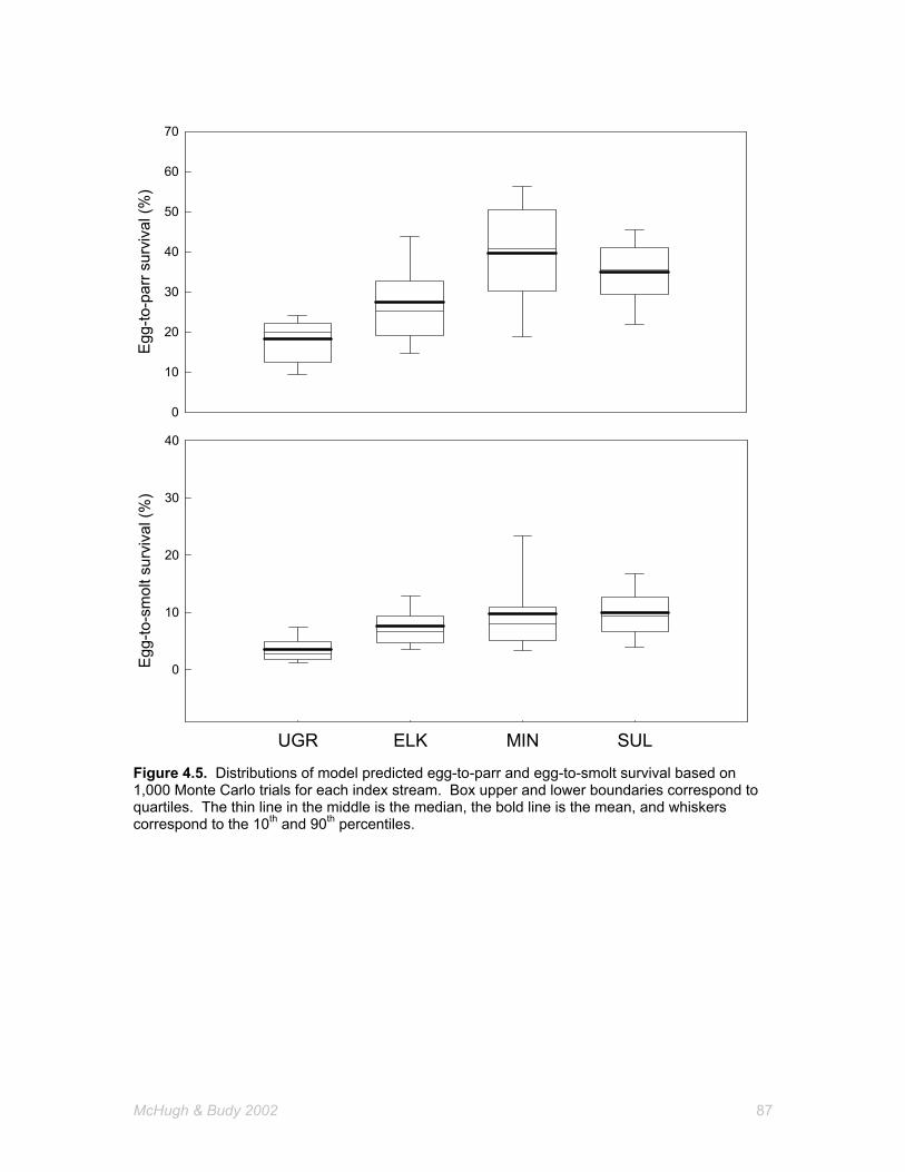
Egg-

to-p

arr s

urvi

val (

%)

0

10

20

30

40

50

60

70

UGR ELK MIN SUL

Egg-

to-s

mol

t sur

viva

l (%

)

0

10

20

30

40

Figure 4.5. Distributions of model predicted egg-to-parr and egg-to-smolt survival based on 1,000 Monte Carlo trials for each index stream. Box upper and lower boundaries correspond to quartiles. The thin line in the middle is the median, the bold line is the mean, and whiskers correspond to the 10th and 90th percentiles.


Observed Survival (%)

0 10 20 30 40

Pred

icte

d Su

rviv

al (%

)

0

10

20

30

40

Egg-to-parrEgg-to-smolt1:1 lin

e

Figure 4.6. Plot of observed vs. predicted egg-to-parr and egg-to-smolt survival rates. The slope of a line between egg-to-parr points is 1.11 (intercept = 25.2) , while the slope between the two egg-to-smolt points is 1.00 (intercept = - 3.7). As there were only two points in both egg-to-parr and egg-to-smolt cases, formal regression hypothesis tests (i.e., F statistic could not be computed) were not conducted.


CHAPTER IV APPENDIX

MODEL COMPUTATIONS Our model computes egg-to-parr (Sparr) and egg-to-smolt survival (Ssmolt) by multiplying habitat-related early life stage survival rates by each other using a product equation. Sparr is computed as (1) Sparr = (SFines)(SincT)(SEMBr)(SsumT) and Ssmolt is computed as (2) Ssmolt = (SFines)(SincT)(SEMBr)(SsumT)(SEMBp) where SFines is survival related to observed fine sediment levels in spawning gravel, SincT is survival related to the average incubation temperature, SEMBr is the survival (summer rearing capacity) due to riffle/run embeddedness, SsumT is the survival through the parr summer rearing period due to stream temperature effects, and SEMBp is the is the overwinter survival (winter rearing capacity) due to riffle/run embeddedness. Fine sediment survival function SFines, or survival to fry emergence, is calculated using a function published in Stowell et al. (1983), based on laboratory work done by Tappel and Bjornn (1983). In their experiments, they incubated chinook salmon embryos in mixtures of gravel with different levels of fine sediment in them and monitored the percent of embryos that survived to fry emergence. From these data the following exponential function was produced: (3) SFines = [92.95 / (1 + e –4.559 + 0.1442 Fines)] / 100 where Fines is the percentage of fine sediments in spawning gravels less than 6.35 mm in diameter. This relationship was generated using fines at depth from core samples, however our dataset consists of surface fines estimates (< 7 mm from pebble counts). We are therefore assuming that surface fines and fines at depth are strongly related. Incubation temperature survival function SincT is calculated using a polynomial function fitted to experimental data published in Murray and McPhail (1988); two additional data points necessary for curve-fitting were taken from Armour (1991). Murray and McPhail (1988) performed laboratory experiments in which chinook salmon (and five other species of Pacific salmon) eggs were incubated in hatchery jars at a five different temperatures (2 - 14 oC; held constant during entire incubation period) and


survival to hatching was monitored. With these data and additional points form Armour (1991) the following second degree polynomial equation was generated: (4) SincT = -0.26 + 0.27Tinc - 0.02Tinc

2 where Tinc is the mean stream temperature during the period between egg deposition (assumed 15 August) and fry emergence (assumed 30 April the following year). The use of this function assumes that a constant incubation temperature (as in Murray and McPhail lab experiments) can be approximated by an average incubation temperature from the field. In addition, using this function in this way implicitly assumes that stream water temperature is a reasonable surrogate for intra-gravel water temperature (which is what eggs actually experience). Violations of these assumptions are likely to cause bias in the predicted SincT. Riffle/run embeddedness survival function SEMBr is calculated using a polynomial function reported in Stowell et al (1983) based on the work of Bjornn et al. (1977). In their experiments, Bjornn et al. (1977) investigated the effects of cobble embeddedness summer rearing capacity in experimental channels (with pool and riffle structure). They added the same number of chinook salmon parr to channels with different levels of embeddedness and monitored how many fish emigrated from the channels over a five day period. The rearing capacity was estimated as the percent of the initial number of fish remaining in the channels after the period. The summer capacity function reported in Stowell et al. (1983) relates percent summer stream capacity to the percent to which cobbles are embedded in run habitat (EMBr, our riffle/run category): (5) SEMBr = [100.0 – 1.79EMBr + 0.0081EMBr2] / 100 Implicit in the manner that this function is applied in our model is that survival patterns related to cobble embeddedness likely reflect the rearing capacity patterns from the Bjornn et al. (1977) experiments. It is important to note that if parr leave a natal stream because of impaired rearing habitat it does not necessarily mean they do not survive beyond that stage. If they are leaving natal streams because of impairment, however, it may be possible to increase the productive capacity in index streams by altering this variable. Summer rearing temperature survival function The survival rate due to the summer rearing temperature, SsumT, is computed using a Weibull function that relates daily survival, Si, to mean daily stream temperature, Tsum, for any given day for the summer rearing period (taken as 1 May through 30 September; deemed to be the period where high temperature


limitation is a possibility). The temperature function decreases daily survival when temperatures exceed an upper temperature tolerance threshold of 17.8 oC:

])0271.27

[( 74.10sumT

i eS -

= (7) This function was fit to published data on the effects of high temperatures on salmon and trout (p < 0.001, F = 6907.71, df= 11; Brett 1952, Coutant 1973, McCormick et al. 1972). SsumT, survival over the summer rearing period, as determined by temperature, is then computed as the product of daily survival for that time period. Below the thermal maximum (17.8 oC), survival is not affected by temperature during this period. Essentially, we modeled only lethal effects of high temperature and therefore did not include sublethal temperature effects (e.g., decreased growth) that might exist below this threshold temperature. SsumT is thus computed using the following product equation:

∏=

=152

1iisumT SS

(6) Pool embeddedness survival function Ssmolt computations include the effect of cobble embeddedness on overwinter survival using a function published in Stowell et al. (1983). This function incorporates the effects of excess fine sediment on the overwintering capacity of a stream (taken as a surrogate for overwinter survival), SEMBp. Based on work done by Bjornn et al. (1977; same design as described above, except during winter) this exponential function relates overwinter capacity for chinook parr to pool embeddedness, EMBp, as: (8) SEMBp = e –0.034EMBp The same assumptions and shortcomings of using this function that were described for summer rearing capacity above apply to this function. Graphical illustrations of each of the habitat-survival relationships appear in Figure 4.2.


ELK AND SULPHUR CREEK 2001 SNORKEL SURVEY DETAILS

Introduction The future of the Pacific salmon (Oncorhynchus spp.) resources of the Snake River Basin is in a precarious state. The recovery of these fish has been a controversial issue, as there are numerous interests at stake. Over the last several years various modeling forums have evaluated recovery options via different management scenarios- particularly hydropower management options. Assessing the overall benefit of recovery measures applied in freshwater spawning and rearing habitat has been focused on to a lesser extent. Currently, we are using modeling techniques to assess the potential for improving the survival of selected Snake River spring/summer chinook salmon stocks through habitat improvements, as proposed in the 2000 Basinwide Recovery Plan (Federal Caucus 2000). Within the framework of this model-based assessment, we are attempting to predict egg-to-parr and egg-to-smolt survival as a direct function of physical habitat variables (e.g., temperature, level of fine sediment in spawning gravel) using published fish-habitat relationships and habitat data collected in selected streams. In order to calibrate and validate model-predicted survival rates, field-based estimates of survival through these life stages are needed. Therefore, during the summer of 2001, chinook parr population estimates were obtained for two streams where physical habitat variables were also measured. This report summarizes the field methods used for estimating population size, the associated computational details, as well as density estimates for other salmonid species residing in the study streams.

Study Site Sulphur Creek and Elk Creek are both important chinook salmon spawning and rearing tributaries in the upper Middle Fork Salmon River Basin in central Idaho (Chapter I, Figure 1.3 and 1.4). Sulphur Creek occurs within the Frank Church- River of No Return Wilderness and has virtually no history of management. It is considered a high quality chinook salmon spawning and rearing stream (Beamesderfer et al. 1997). Elk Creek has a more extensive history of management, primarily in the form of livestock grazing (Beamesderfer et al. 1997). Elk Creek is considered a moderate quality spawning and rearing stream (although Bear Valley/Elk Creek combined stock is considered poor). Chinook salmon population trend data (i.e., redd counts) have been collected in both streams for nearly fifty years. Estimates of chinook summer parr population size and egg-to-parr survival, however, are limited for both streams (Kiefer et al. 1992). Field sampling in both streams was limited to those reaches that are surveyed for chinook redds annually (i.e., traditional index areas and additional reaches surveyed during redd counts; as in Elms-Cockrum 2001).


Methods

Snorkel surveys were conducted within the framework of a ten percent stratified systematic sample based on channel units (pools and riffles, according to definitions of Henderson et al., in review). Channel units were limited to two classes because increased complexity in habitat classification schemes can result in increased error (Roper and Scarnecchia 1995). Strata were established on the basis of stream channel characteristics (Table A.1; channel type, wetted width, etc.), as these variables tend to influence fish distribution and abundance (e.g., Petrosky and Holubetz 1988). Before field sampling occurred, our snorkel crew received training from Idaho Department of Fish and Game (IDFG) personnel in Lewiston, ID. Training emphasized accurate identification of fish species and size estimation. In the field, snorkel counts were limited to the time period between 10:00 and 18:00 when minimum recommended visibility (>3 m) and temperature (>9 oC) criteria were met or exceeded (Thurow 1994). Habitat surveys were also conducted in each unit that was snorkeled, though details are presented in another report (see Chapter II section for details). In each channel unit that was snorkeled, observers proceeded in an upstream direction while scanning for fish across their assigned lane, such that the entire channel was surveyed. All chinook salmon were counted as either age-0+ (<100 mm), age-1+ (>100 mm), or adult (Anderson et al. 2001). Juvenile steelhead/rainbow trout (Oncorhynchus mykiss) were counted and classified as age-1+ (76 – 127 mm) and age-2+ (> 127 mm), according to the size classes of the IDFG General Parr Monitoring program. Details on the level of detail recorded for all fish species encountered appear in Table A.2. The dimensions of channel units snorkeled were also measured so that the density (fish / 100 m2) of fish species could be determined. The complete population size of chinook parr, age-1+, and age-2+ steelhead/rainbow trout in each of the study reaches was estimated. Population estimation procedure Sampling was done under a systematic design assuming the absence of any spatial periodicity of fish abundance; therefore, we applied estimation procedures based on a random sampling approach. Population estimation procedures for quadrat counts were employed for the estimation of fish abundance, for each habitat type (all equations are from Krebs 1999, unless noted otherwise). Initially, we explored the possibility of estimating the population size from our snorkel counts using four different approaches, but ultimately decided on a modified version of the Hankin and Reeves (1988) estimators. The following discussion details how we arrived at our population estimates.


First, in order to meet the assumption of equal area of habitat units, we adjusted the count (xiadj) in each site by the mean area of all sites (similar to adjustment of Nemeth et al. 1996) using equation 1,

(1) i

iadji z

zxx = ,

where xi is the number of fish of fish in unit i, zi is the area of unit i, and z is the mean area of all sites snorkeled. From this we computed the mean number of fish per site (Hankin and Reeves 1988)

(2) n

xx

n

iadji∑

== 1

and its associate variance, s , 2ˆx

(3) 1

/)(ˆ 1

2

1

2

2

−

−=

∑∑==

n

nxxs

n

iiadj

n

iiadj

x .

With the mean number of fish per site estimated, the population total for a given habitat type (a) in a given stratum (h) is: (4) xNXha =ˆ . The variance of the total population size for habitat a in stratum h was computed as:

(5) )1()ˆ( 22

Nns

nNXVar xha −= .

The total population estimate for the entire study reach is then:

(6) . ∑ ∑= =

=l

hha

aXX

1

2

1ˆˆ

Since the total and variance estimates are from independent samples, the variance for the population total is additive for habitat types and strata (Dolloff et al. 1993). The variance of the total is:


(7) =)ˆ(XVar )ˆ(1

2

1∑ ∑= =

l

hha

aXVar

and the standard error is

(8) )ˆ()ˆ( XVarXSE = . Ninety percent confidence intervals were calculated using standard error of the total, the appropriate degrees of freedom, and α/2. We calculated degrees of freedom (df) using Cochran’s (1977 cited in Krebs 1999) formulation:

(9)

∑

∑

=

=

−

=l

h h

hh

l

hhh

nsg

sgdf

1

2221

2

1)(

, where

(10) h

hhhh n

nNNg )( −= .

In order to evaluate the relative precision of these population estimates, we also calculated relative confidence intervals as in Nemeth et al. (1996). It should be noted that our confidence intervals are a minimum estimate of the level of uncertainty around the population total, as they do not include first-stage variance component of total variance (i.e., variance between repeated counts in a given unit). The second-stage variance (i.e., variance between counts in different units), however, is the greatest contributor to the total variance (Hankin and Reeves 1988), as snorkel counts of stream salmonids within the same unit are reasonably precise (Schill and Griffith 1984). Estimating chinook egg-to-parr survival Using our chinook parr population estimates, we computed egg-to-parr survival using the number of chinook redds for brood year 2000 (B. Horton, IDFG, unpublished data), an assumed one female per redd, and a fecundity estimate of 5,900 eggs/female (Petrosky and Holubetz 1988). In addition to these estimates, we compiled available estimates of egg-to-parr survival for Elk and Sulphur creeks for comparitive purposes.


Results

Field surveyors snorkeled 35 channel units (22 pools and 13 riffles) in Sulphur Creek and 66 (44 pools and 22 riffles) channel units in Elk Creek. The population estimates for chinook parr and steelhead/rainbow in the study are shown in Table A.3. The chinook parr population estimate in Elk Creek was nearly six times that of Sulphur Creek. There was slightly more error around the Sulphur estimate when compared to that of Elk Creek (relative CI 45% and 29%, respectively). The estimated age-1+ and age-2+ steelhead/rainbow population estimates for the study reaches were considerably higher for Sulphur Creek, when compared to Elk Creek. Variance around steelhead/rainbow population estimates were considerably greater than for chinook salmon (mean relative CI 75% and 37%, respectively).

Chinook egg-to-parr survival estimates for both streams were similar to those available from previous studies despite different population estimation methods (Table A.4). Egg-to-parr survival estimated in this study for Sulphur Creek (8.7%) was nearly four times that of Elk Creek (2.0%). Elk and Sulphur creeks were composed of slightly different fish communities, however overall salmonid density (excluding mountain whitefish, Prosopium williamsoni, and adult chinook) was similar for both streams (Figure A.1). Densities of all fish species varied by habitat type and strata (Table A.5).

Conclusions

Snorkeling proved to be an effective means for estimating the abundance of chinook salmon parr and ultimately egg-to-parr survival in the study streams. The close agreement between our survival estimates and the few available from previous studies in Elk and Sulphur creeks (Table A.4) suggests two things. First, it suggests that snorkeling is a reasonable approach to estimating parr population size. Additionally, it suggests that there exists a consistent disparity between survival in these two streams, although this conclusion is somewhat sensitive to parr population estimation procedures employed (e.g., Sulphur Creek estimates obtained from Nemeth et al. 1996 parr data; Table A.4). The apparent lower survival in Elk Creek is possibly attributable to differences in habitat quality, however it is believed that some proportion of chinook fry leave this stream in the spring and rear in lower Bear Valley Creek and the mainstem Middle Fork Salmon River, though this has not yet been quantified (C. Petrosky, IDFG, personal communication). Nonetheless, if procedures are applied consistently from year to year in the same manner, inter-annual and inter-stream comparisons are appropriate. Population estimates for age-1+ and age-2+ steelhead/rainbow in study streams, while provided in this report, may be somewhat misleading. As field sampling was primarily for estimating chinook parr abundance, snorkel counts were confined to the main chinook spawning/rearing reach of both streams.


Therefore, we did not effectively sample the portion of both watersheds where juvenile steelhead/rainbow typically rear (i.e., higher gradient reaches, with the exception of stratum 1 in Sulphur Creek). This is possibly why variance around steelhead/rainbow estimates was considerably higher than for chinook parr. Density data for steelhead/rainbow and other salmonids from this study, however, are useful for monitoring purposes. Recommendations for summer 2002 In order to assess the relative utility of estimating parr population size and egg-to-parr survival in these two streams from snorkel data, we believe snorkeling both streams again is necessary. This will enable us to determine whether or not we can consistently estimate egg-to-parr survival. To improve our chinook parr estimates (i.e., reduce variance around estimates) we also propose sampling riffles at a lower intensity and pools at a higher intensity due to the relative contribution to total variance from these two habitats. Finally, if additional data on steelhead/rainbow populations in the study streams are desired, we will need to expand our snorkel efforts other areas in both streams.


Table A.1. Strata characteristics for study streams.

Stream Stratum Channel

Typea km

surveyed No.

PoolsNo.

Riffles% Area Pools

% Area Riffles

Wetted Width (m)

Elk Ck. 1 C 15.7 184 78 87.0 13.0 11.0 Elk Ck. 2 C 13.8 262 135 82.6 17.4 7.6

total 29.5 Sulphur Ck. 1 Bb 5.5 28 26 12.8 87.2 12.2 Sulphur Ck. 2 C 8.7 195 104 64.5 35.5 7.6

total 14.2 a. Rosgen (1985) classification system as delineated by IDFG General Parr Monitoring Program. b. Predominantly a B-channel section, with short intervening C-channel reach.

Table A.2. Fish species encountered and level of detail recorded during observation.

Species Count or P/A Age or Size

Chinook Salmon Parr Count Age Chinook Salmon Adult Count neither Steelhead/rainbow Count Size Cutthroat Trout (Oncorhynchus clarki) Count Size Mountain Whitefish (Prosopium williamsoni) Count neither Brook Trout (Salvelinus fontinalis) Count Size Bull Trout (S. confluentus) Count Size Miscellaneous salmonid fry P/A neither Sculpin (Cottus spp.) P/A neither Tailed Frog (Ascaphus truei) P/A neither


Table A.3. Population estimates, upper and lower confidence bounds (UCB and LCB), and relative confidence intervals (CI) for selected species in Elk and Sulphur Creek for summer of 2001.

Chinook Steelhead/rainbow

Stream Stratum / Habitat Age-0+ Age 1+ Age 2+ Elk Creek 1 Pool 2,899 86 40

1 Riffle 205 38 0 2 Pool 8,780 135 0 2 Riffle 297 0 0 Stream Total 12,182 259 40 90% UCB 15,681 443 86 90% LCB a 8,682 75 4 Relative CI (%) b 29 71 102

Sulphur Creek 1 Pool 85 62 22 1 Riffle 104 430 185 2 Pool 2,165 698 88 2 Riffle 223 94 0 Stream Total 2,578 1,285 295 90% UCB 3,749 1,881 517 90% LCB a 1,406 689 32 Relative CI (%) b 45 46 82

a. Steelhead/rainbow LCB truncated at minimum adjusted count so as not to have negative LCB. b. Relative CI = (CI / population estimate) x 100

Table A.4. Egg-to-parr survival (S) estimates for Elk and Sulphur creeks for brood year 2000 and from past studies.

Sulphur Creek Elk Creek

Study

Petrosky and Holubetz (1988)b

Nemeth et al. (1996)

This study

Petrosky and Holubetz (1988)b

This study

Brood Year 1988 1993b 1993c 2000 1984 1985 1986 2000Parr Estimate 64,197 9,266 45,976 2,578 6,559 1,885 2,581 12,18290% UCB . 11,953 58,390 3,749 . . . 15,68190% LCB . 6,579 33,562 1,406 . . . 8,682Redds 140 84 84 5 27 28 55 103 S (%) a 7.8d 1.9 9.3 8.7 4.1 1.1 0.8 2.0 S (UCB) . 3.6 11.8 12.7 . . . 2.6 S (LCB) . 2.0 6.8 4.8 . . . 1.4

a. Assuming 1 redd/female, 5900 eggs/female (Petrosky and Holubetz 1988). b. From population estimate obtained by expanding representative reach into total estimate. c. Similar to our estimation procedure. d. Parr estimate not in original report, calculated from survival estimate reported (11.6%, based on 1.5

redds/female, 5,900 eggs/female). Survival reported here assumes 1 redd/female.


Table A.5. Mean (standard error) density of fish species encountered during summer 2001 snorkel surveys by habitat and stratum in study streams.

Fish Density (Fish / 100m2)

Stream Stratum /

Habitat Type Chinook Parr Steelhead/ Rainbow 1+

Steelhead/ Rainbow 2+

Cutthroat Trout

Mountain Whitefish Bull Trout Brook Trout

All Salmonids (excl. Whitefish and

Adult chinook) Chinook AdultSulphur 1 Pools 0.91 (0.91) 0.66 (0.32) 0.23 (0.13) 0.47 (0.26) 1.09 (0.58) 0.00 (0.00) 0.00 (0.00) 3.64 (1.37) 0.00 (0.00) Creek 1 Riffles 0.16 (0.14) 0.67 (0.37)

0.29 (0.14) 0.06 (0.03) 0.62 (0.45) 0.00 (0.00) 0.00 (0.00) 2.20 (1.17) 0.00 (0.00) 2 Pools 4.27 (1.38) 1.38 (0.46) 0.17 (0.07) 0.74 (0.36) 0.76 (0.50) 0.34 (0.31) 0.00 (0.00) 9.20 (2.83) 0.05 (0.04) 2 Riffles 0.80 (0.31) 0.34 (0.23) 0.00 (0.00) 0.89 (0.38) 0.50 (0.17) 0.06 (0.06) 0.00 (0.00) 3.32 (1.24) 0.00 (0.00)

1 & 2 Pools 3.81 (1.22) 1.28 (0.40) 0.18 (0.06) 0.71 (0.31) 0.80 (0.44) 0.29 (0.26) 0.00 (0.00) 8.44 (2.48) 0.05 (0.04) 1 & 2 Riffles

0.65 (0.25) 0.41 (0.19) 0.07 (0.04) 0.70 (0.30) 0.52 (0.16) 0.05 (0.05) 0.00 (0.00) 3.06 (0.98) 0.00 (0.00)

All Units 2.64 (0.81) 0.96 (0.27) 0.14 (0.04) 0.70 (0.22) 0.70 (0.28) 0.20 (0.17) 0.00 (0.00) 6.44 (1.65) 0.03 (0.02)

Elk 1 Pools 1.73 (0.77) 0.05 (0.03) 0.02 (0.02) 0.21 (0.11) 1.29 (0.78) 0.01 (0.01) 0.23 (0.13) 2.26 (1.02) Creek 1 Riffles 0.82 (0.45) 0.15 (0.12) 0.00 (0.00) 0.00 (0.00) 0.00 (0.00) 0.00 (0.00) 0.00 (0.00) 0.98 (0.55) 0.00 (0.00)

2 Pools 9.73 (1.95) 0.15 (0.11) 0.00 (0.00) 0.05 (0.03) 1.30 (0.51) 0.01 (0.01) 0.14 (0.06) 10.07 (1.99) 0.24 (0.18) 2 Riffles 1.56 (1.02) 0.00 (0.00) 0.00 (0.00) 0.00 (0.00) 0.00 (0.00) 0.00 (0.00) 0.00 (0.00) 1.56 (1.02) 0.00 (0.00)

1 & 2 Pools 6.46 (1.33) 0.11 (0.06) 0.01 (0.01) 0.12 (0.05) 1.29 (0.43) 0.01 (0.01) 0.17 (0.06) 6.88 (1.37) 0.31 (0.18) 1 & 2 Riffles

1.29 (0.66) 0.06 (0.04) 0.00 (0.00) 0.00 (0.00) 0.00 (0.00) 0.00 (0.00) 0.00 (0.00) 1.35 (0.67) 0.00 (0.00)

All Units 4.73 (0.96) 0.09 (0.05) 0.01 (0.00) 0.08 (0.00) 0.86 (0.30) 0.01 (0.00) 0.12 (0.04) 5.03 (0.99) 0.21 (0.12)

0.42 (0.37)


0.00

1.00

2.00

3.00

4.00

5.00

6.00

7.00

8.00

9.00

10.00

11.00

ChinookParr

STH/RBT1+

STH/RBT2+

Cutthroat Whitefish Bull Trout BrookTrout

AllSalmonids

ChinookAdult

Den

sity

(Fis

h / 1

00 m

2 )

Elk Creek

Sulphur Creek

Figure A.1. Mean fish density in pool habitats (combined strata) in Elk and Sulphur Creeks, summer 2001. Error bars correspond to one standard error.


References Anderson, J.L., K. Bacon, and K. Denny. 2001. Salmon River habitat enhancement: annual

report 2000. Shoshone-Bannock Tribes annual report to U.S. Department of Energy-Bonneville Power Administration, Portland, Oregon.

Armour, C.L. 1991. Guidelines for evaluating and recommending temperature regimes to protect fish. U.S. Fish and Wildlife Service. Fort Collins. Biological Report 9(22). 13pp.

Baker, P.F., T.P. Speed, and F.K. Ligon. 1995. Estimating the influence of temperature on the survival of chinook salmon smolts (Oncorhynchus tshawytscha) migrating through the Sacramento – San Joaquin River Delta of California. Canadian Journal of Fisheries and Aquatic Sciences 52:855-863.

Beamesderfer, R. C. P., H. A. Schaller, M. P. Zimmerman, C. E. Petrosky, O. P. Langness, and L. LaVoy. 1997. Spawner-recruit data for spring and summer chinook salmon populations in Idaho, Oregon, and Washington. Draft report to: Marmorek, D. R., and C. N. Peters (eds.). J. Anderson, R. Beamesderfer, L. Botsford, J. Collie, B. Dennis, R. Deriso, C. Ebbesmeyer, T. Fisher, R. Hinrichsen, M. Jones, O. Langness, L. LaVoy, G. Matthews, C. Paulsen, C. Petrosky, S. Saila, H. Schaller, C. Toole, C. Walters, E. Weber, P. Wilson, M. P. Zimmerman. 1998. Plan for Analyzing and Testing Hypotheses (PATH): Retrospective and Prospective Analyses of Spring/Summer Chinook Reviewed in FY 1997. Compiled and edited by ESSA Technologies Ltd., Vancouver, B. C.

Bjornn, T.C. 1971. Trout and salmon movements in two Idaho streams as related to temperature, food, stream flow, cover, and population density. Transactions of the American Fisheries Society 100:423-438.

Bjornn, T.C., M.A. Brusven, M.P. Molnau, J.H. Milligan, R.A. Klamt, E. Chacho, and C. Schaye. 1977. Transport of granitic sediment in streams and its effects on aquatic life. University of Idaho, Forest, Wildlife, and Range Experiment Station Bulletin 17, Moscow, Idaho.

Bradford, M.J. 1995. Comparative review of Pacific salmon survival rates. Canadian Journal of Fisheries and Aquatic Sciences 52:1327-1338.

Brett, J. R. 1952. Temperature tolerance in young Pacific salmon, genus Oncorhynchus. J. Fish. Res. Bd. Canada 9:265:309.

Chapman, D.W. 1988. Critical review of variables used to define effects of fines redds of large salmonids. Transactions of the American Fisheries Society 117:1-21.

Coutant, C.C. 1973. Effects of thermal shock on vulnerability of juvenile salmonids to predation. Journal of the Fisheries Research Board of Canada 30:965-973.

Dolloff, C.A., D.G. Hankin, and G.H. Reeves. 1993. Basinwide estimation of fish populations in streams. Gen. Tech. Rep. SE-83. Asheville, NC: U.S. Department of Agriculture, Forest Service, Southeastern Forest Experiment Station. 25 pp.

Elms-Cockrum, T.E. 2001. Salmon spawning ground surveys, 1999. Idaho Department of Fish and Game. Pacific Salmon Treaty Program: Award No. NA47FP0346. IDFG 01-10, March 2001. 26 pp. plus appendices.

Federal Caucus 2000. Final basinwide salmon recovery strategy. December 21, 2000. Griffith, J.S., and R.W. Smith. 1993. Use of winter concealment cover by juvenile cutthroat and

brown trout in the South Fork of the Snake River, Idaho. North American Journal of Fisheries Management 13:823-830.

Groot, C., and L. Margolis. 1991. Pacific salmon life histories. University of British Columbia Press, Vancouver, B.C., Canada.

Hankin, D. G. and G. H. Reeves. 1988. Estimating total fish abundance and total habitat area in small streams based on visual estimation methods. Canadian Journal of Fisheries and Aquatic Sciences 45:834-844.

Henderson, R., E. K. Archer, and J. L. Kershner. In review. Effectiveness monitoring protocols for streams and riparian areas -sampling protocol for stream parameters.

Hillman, T.W., J.S. Griffith, and W.S. Platts. 1987. Summer and winter habitat selection by juvenile chinook salmon in a highly sedimented Idaho stream. Transactions of the American Fisheries Society 116:185-195.

Kareiva, P., M. Marvier, and M. McClure. 2000. Recovery and management options for spring/summer chinook salmon in the Columbia River Basin. Science 290:977-979.


Kiefer, S.A., M. Rowe, and K. Hatch. 1992. Stock summary report for Columbia River anadromous salmonids, volume V: Idaho subbasins. Columbia River Coordinated Information System, Final Report to U.S. Department of Energy-Bonneville Power Administration, Portland, Oregon.

Kondolf, G.M. 1993. Lag in stream channel adjustment to livestock exclosure, White Mountains, California. Restoration Ecology 1:226-230.


Krebs, C.J. 1999. Ecological Methodology. 2nd edition. Harper Collins, New York. McCormick, J.H., K.E.F. Hokanson, and B.R. Jones. 1972. Effects of temperature on growth and

survival of young brook trout, Salvelinus fontinalis. Journal of the Fisheries Research Board of Canada 29:1107-1112.

McCullough, D.A. 1999. A review and synthesis of effects of alterations to the water temperature regime on freshwater life stages of salmonids, with special reference to chinook salmon. Report to the U.S. Environmental Protection Agency, Seattle, Washington.

Murray, C.B. and J.D. McPhail. 1988. Effect of incubation temperature on the development of five species of Pacific salmon (Oncorhynchus) embryos and alevins. Canadian Journal of Zoology 66:266-273.

Mundy, P.R. 1999. Status and expected time to extinction for Snake River spring and summer chinook stocks: the doomsday clock and salmon recovery index models applied to the Snake River Basin. Report to Trout Unilimited, Portland, Oregon.

Nemeth, D., K. Plaster, K. Apperson, J. Brostrom, T. Curet, and E. Brown. 1996. Idaho supplementation studies annual report 1994. Idaho Department of Fish and Game annual report to U.S. Department of Energy-Bonneville Power Administration, Portland, Oregon.

NMFS (National Marine Fisheries Service). 1992. Endangered and threatened species; threatened status for Snake River spring/summer chinook salmon, threatened status for Snake River fall chinook salmon. Federal Register [Docket No. 910647-2043, 22 April 1992] 57(78):14,653-14,662.

Peters, C.N., D.R. Marmorek. 2001. Application of decision analysis to evaluate recovery actions for threatened Snake River spring and summer chinook salmon (Oncorhynchus tshawytscha). Canadian Journal of Fisheries and Aquatic Sciences 58:2431-2446.

Petrosky, C.P., and T. Holubetz. 1988. Idaho habitat evaluation for off-site mitigation record: annual report 1987. Idaho Department of Fish and Game annual report to U.S. Department of Energy-Bonneville Power Administration, Portland, Oregon.

Raleigh, R. F., W. J. Miller, and P. C. Nelson. 1986. Habitat suitability index models and instream flow suitability curves: chinook salmon. U.S. Fish Wildl. Serv. Biol. Rep. 82(10.122). 64 pp.

Reiser, D.W., and R.G. White. 1988. Effects of two sediment size-classes on survival of steelhead and chinook salmon eggs. North American Journal of Fisheries Management 8:432-437.


Rosgen, D. L. 1985. A stream classification system. North American Riparian Conference. Tucson, Arizona. April 16-18, 1985.

Schill, D.J., and J.S. Griffith. 1984. Use of underwater observations to estimate cutthroat trout abundance in the Yellowstone River. North American Journal of Fisheries Management 4:479-487.

Shepard, B. B., S. A. Leathe, T. W. Weaver, and M. D. Enk. 1984. Monitoring levels of fine sediment within tributaries to Flathead Lake, and impacts of fine sediment on bull trout recruitment. Paper presented at the Wild Trout III symposium. Yellowstone National Park, Wyoming. 11 pp.

Skille, J., and J. King. 1989. Proposed cobble embeddedness sampling procedure. Unpublished report. 10 pp.

Stowell, R., A. Espinosa, T.C. Bjornn, W.S. Platts, D.C. Burns, and J.S. Irving. 1983. Guide for predicting salmonid response to sediment yields in Idaho Batholith watersheds. U.S.



Forest Service, Northern Region, Missoula, Montana, and Intermountain Region, Ogden, Utah.

Tappel, P.D., T.C. Bjornn. 1983. A new method of relating size of spawning gravel to salmonid embryo survival. North American Journal of Fisheries Management 3:123-135.

Thurow, R. F. 1994. Underwater methods for study of salmonids in the Intermountain West. General Technical Report INT-GTR-307. Ogden, Utah: U. S. Department of Agriculture, Forest Service, Intermountain Research Station. 28 pp.

Weaver, T.M., and J.J. Fraley. 1993. A method to measure emergence success of westslope cutthroat trout fry from varying substrate compositions in a natural stream channel. North American Journal of Fisheries Management 13(4):817-822.


snake river spring/summer chinook … river spring/summer chinook salmon habitat feasibility study...

Documents