* neal.brock@4DTechnology.com, phone 520-294-5600, 4DTechnology.com

Snap-shot Imaging Polarimeter: Performance and Applications

Neal J. Brock*, Charles Crandall, James E. Millerd

4D Technology Corporation, 3280 E. Hemisphere Loop Unit 146, Tucson,

AZ, USA 85706-5039

ABSTRACT

A camera capable of obtaining single snap-shot, quantitative, polarimetric measurements is investigated to determine

performance characteristics. The camera employs a micropolarizer array with linear polarizers oriented at 0, 45, 90, and,

135 degrees. Micropolarizer arrays with elements as small as 7.4 microns and arrays as large 4 million pixels have been

fabricated for use across the visible spectrum. The pixelated polarization camera acquires the four polarization

orientations in a single video frame, which enables instantaneous measurements of the linear Stokes parameters.

Examples of calibration methods and the results of controlled experiments are presented. Error sources and methods for

minimizing them are discussed and demonstrated. A practical example of measuring stress induced birefringence is

demonstrated.

Keywords: polarimetry, micropolarizer array, pixelated polarizer, snap shot imaging polarimeter

1. INTRODUCTION

Imaging polarimetry has a variety of emerging applications such as 3D shape measurement, remote sensing, target

discrimination, haze removal, bio-tissue imaging, and polarization microscopy.1 The demand for greater spatial and

temporal resolution in imaging polarimeters inspired the development of micropolarizer arrays capable of matching the

size and pitch of camera sensors. The concept of a pixel-matched polarizer array was described by Chun, et. al. in 1994

for use at infrared wavelengths.2 The approach permits single frame, quantitative measurements without the deleterious

effects of vibration and motion. Compared with multi-camera imaging, the pixel-matched polarizer is very compact and

light-weight and permits the use of conventional lenses where the optics can be very close to the sensor. A camera with

a pixel-matched micropolarizer array was demonstrated in 1999 by Nordin3 et. al., and used in an imaging polarimetry

system. Later, Millerd4 et. al. developed a pixelated camera for use in a dynamic imaging interferometry system. Since

then, the pixelated polarizer camera (also known as the PolarCam™) has been the core element to 4D Technology’s

dynamic phase measurement technology where it has been used for making commercial dynamic interferometers since

2004. With hundreds of systems installed in facilities around the world, it has proven to be a rugged and reliable

platform.

The PolarCam is well characterized for use in interferometers, where it has demonstrated sub-angstrom repeatability for

measuring the shape and surface texture of optics and precision engineered surfaces. However, the parameters of interest

in imaging polarimetry are somewhat different owing to the different optical configuration and intended application. In

this paper we review details of 4D Technology's snap-shot imaging polarimeter, discuss the main factors that influence

its performance, measure the performance of a 2 megapixel camera using metrics that are appropriate for polarimetry

systems, and discuss the practical application of measuring stress-induced birefringence in glass.

2. PIXELATED POLARIZER CAMERA

The PolarCam utilizes a wiregrid micro-polarizer array, fabricated using nanoscale patterning of a metal grating with

sub-wavelength spacing on a thin transparent glass substrate. The wiregrid polarizer is characterized by high

transmission, high extinction, and a broad spectral and angular bandwidth. The wiregrid micro-polarizer array is

produced in a lithographic process that produces a pattern of polarizers with four discrete polarizations (0, 45, 90, 135

degrees) known as a super pixel (see Figure 1) that is repeated over the entire array. The size and frequency or spacing of

the individual micropolarizer element is chosen to match exactly the size and pitch of the desired camera sensor.

Polarization crosstalk is kept to a minimum by leaving an unpatterned border area around each individual polarizer

element and by mounting the micropolarizer substrate directly to the camera CCD microlens surface. Cross-talk can also

be minimized by careful choice of the pixelated polarizer ordering. The polarizer ordering diagramed in Figure 1 was

shown to minimize cross-talk for interferometry in reference 5 and for polarimeters in reference 6.

The micropolarizer array can be used over a wavelength range from 300nm to 1µm. At a wavelength of 550nm, the

transmission of the pixelated polarizer can be as high as 80% and the extinction ratio can be greater than 50:1.7 The

cameras can be used with either coherent or incoherent light. Three standard pixelated cameras are available in the same

physical housing (shown in Figure 2) with pixel resolutions of 1, 2, and 4 Megapixels. The cameras utilize the GigE

interface and interline transfer CCD sensors with 7.4 micron pixels.

3. POLARIMETRY MEASUREMENTS

The Stokes vector is a convenient method to describe the polarization state of a light beam because each element can be

conveniently measured. Combined with the Mueller matrix, which describes the transfer function of an optical device,

one can easily compute the output polarization state of a light beam impinging on multiple elements via matrix

multiplication. The Stokes vector is fully characterized from 6 measurements of the light beam according to:8

Figure 2. Compact 1Mpixel PolarCam (46x46x60 mm) with C-mounted lens.

Figure 1. The diagram of the pixelated micropolarizer array shows the multiple polarization orientations that

comprise the super pixel cell. The central image is an SEM of the micropolarizer array (courtesy of Moxtek Inc.).

(1)

where I0, I90, I45, I135, are the measured intensities of the linear polarization components 0, 90, 45, 135 degrees

respectively, and ILHC, IRHC are the measured circular polarization components for left hand circular, and right hand

circular, respectively. The micropolarizer array described here measures the 4 linear polarization components and thus

can be used to determine s0, s1, s2 at each super pixel.6 A general purpose polarimeter would ideally measure all 4 Stokes

parameters (equivalent to all 6 intensity components); however, for a large number of applications the first three

parameters are sufficient.

The Mueller matrix formalism can be used to describe the transformation of the Stokes vector through any optical

system according to:

(2)

Where mx,y are the Mueller matrix coefficients and S’ denotes the transformed Stokes vector with parameters s’.

Polarimetry applications can be broadly classified into two categories: active and passive illumination. Passive

illumination is typically measurement of scenes involving reflected or scattered sunlight, for example identifying man-

made metallic objects in a background of vegetation, or removal of haze. Sunlight is randomly polarized and light

scattered or reflected from natural objects tends to impart only a linear polarization. Therefore, for many passively

illuminated scenes, the assumption can be made that ILHC = IRHC, and s3 = 0 and the linear Stokes parameters provide

adequate characterization.

Active illumination affords the opportunity to better control the experimental conditions and can simplify the

calculations. If the active illumination is completely polarized, and there are no mechanisms within the optical setup to

generate unpolarized light (i.e. the randomly polarized element is zero) then the following relationship between the

Stokes parameters holds

2

3

2

2

2

1

2

0 ssss ++= (3)

Thus, by measuring the first three components it is possible to fully characterize the Stokes parameters. In particular, the

circular component can be found from:

)( 2

2

2

1

2

0

2

3 ssss +−= (4)

A convenient normalization method is to divide the Stokes parameters by the total intensity s0 and represent them as

dimensionless quantities, S1, S2, S3, which range from -1 to 1. Note that S0 = 1 by definition so that equation 4 becomes

)(1 2

2

2

1

2

3 SSS +−= . (5)

The normalized Stokes parameters can still be used with the Mueller matrix as before.

For general purpose measurements that may include both random and circular components, additional optical

components such as a waveplate can be used to determine s3; however, the simplicity and instantaneous imaging

capability of the pixelated camera are usually sacrificed.

Two useful parameters in polarimetry are the degree of linear polarization,

. (6)

and the angle of linear polarization,

(7)

DoLP can be regarded as the fraction of incident light intensity in the linear polarization state while the AoLP is the

polarization angle of the incident light relative to the detector axis. The pixelated camera offers an extremely simple

configuration for measuring the instantaneous polarization data for determining both DoLP and AoLP, which is a

significant advantage over other polarimetry methods. In this paper we discuss limitations on measuring these two

parameters and provide actual performance data.

4. MEASUREMENT PERFORMANCE CONSIDERATIONS

There are several factors to consider when employing the micropolarizer camera for quantitative measurements. In this

section we discuss some of the relevant considerations and discuss their potential impact. Four areas to consider are

effective spatial resolution, electronic crosstalk, pixel-to-pixel uniformity, and random noise.

4.1 Spatial Resolution

One consideration when employing the micropolarizer camera is its effective lateral resolution. The mosaic pattern of

polarizers necessarily reduces the effective spatial resolution relative to the pitch of the native detector array; however,

the actual performance depends both on the processing algorithms employed and the spatial frequency distribution of

information between the intensity and polarization domains of the scene being imaged. It is convenient to think of the

information content in the spatial frequency domain as shown in Figure 3. For simplicity this is shown along only one

linear dimension. The periodic nature of the polarizer pattern creates an effective bias in spatial frequency of the

polarization signal relative to the underlying intensity distribution. The base spatial frequencies of the intensity signal

(S0) and the polarimetry signals (S1 and S2) are separated by the Nyquist frequency (fN=1/2N). Depending on the actual

measurement conditions, the spatial frequency content of the S0 and S1, S2 maps may overlap. For example, when

imaging a scene with sharp edges such as buildings the rapid transition at the edge produces a high frequency signal that

will leak into the polarization channels and create a cross-talk due to spectral overlap. The ideal measurement scenes

have well separated polarization and intensity content, although this is not always practical.

Figure 3. Distribution of S0, S1 and S2 signals in the spatial frequency domain. Both the optical imaging configuration

and the processing algorithm can be used to mitigate signal overlap between S0, S1 and S2.

There are several different methods for extracting the polarization signal and Stokes parameters that can have a

significant effect on the effective spatial resolution and effects of spectral overlap. The most straight-forward method of

processing data is to use the so-called super pixel or parsed approach. Using the parsed approach, calculation of the

Stokes parameters at each super pixel results in a polarization image that is ¼ of the raw data, as shown in Figure 4a,

where A, B, C, and D represent the polarizations, 0, 45, 90, and 135 degrees, respectively. Thus, the final array has half

the spatial resolution of the original array. Several authors have shown that resolution can be improved using different

groupings of adjacent pixels.9 By convolving a 2x2, or 3x3 pixel kernel across the array as shown in Figure 4b, both the

spatial resolution of the data and the effects of spectral overlap can be improved. Spatial frequency overlap has been

extensively studied by Tyo, et. al. and several other algorithms have been proposed to minimize cross-talk. Note that the

level of cross-talk between S0 and S1, S2, depends on the actual scene being imaged, thus, it is not possible to directly

measure inherent cross-talk in a general way. Furthermore, the increasing pixel count on high performance detectors can

effectively offset the reduction in resolution while still maintaining a simple imaging configuration.

1.2. Local Signal Cross-talk

In addition to the inherent coupling of S0 with S1 and S2 terms described in 4.1, there can also be signal cross-talk due to

local coupling of both the optical and electrical signals between adjacent pixels. For example, electrical blooming and/or

smear are well known phenomena in CCDs where signals in adjacent pixels combine with each other. These are

typically dependent on factors such as the camera integration time and the electrical clocking signals. In general, smear

is reduced with longer exposure times. Therefore, it is desirable to use an exposure time that is just adequate to freeze

out desired motion, but not shorter.

Optical cross-talk can occur when illuminating with large angles, so that light incident on the mask intersects adjacent

pixels. Optical cross-talk will increase inversely with the F/# of the optical imaging system. In addition, the resolution

Figure 4. a) Diagram of micropolarizer super pixel and corresponding phase resolution. b) Diagram showing how

2x2 convolution kernel achieves higher resolution.

of the optical image will also increase inversely with F/#. Setting the F/# too low will result in significant high spatial

frequency information that will couple between S0 and the S1, and S2 channels. Therefore, it is desirable to set the F/# to

a value equal to or higher than the value that matches the ½ Nyquist frequency of the detector.

1.3. Pixel-to-pixel uniformity

Image sensor pixels and micro-grid polarizer pixels inherently have response, contrast, and transmission variations

introduced during the manufacturing process. These variations could manifest as gain and offset in the CCD pixel, and

consequently as errors in the calculated S parameters, AoLP and DoLP. One method to correct for these imperfections is

through the “flat-fielding technique”. To perform a flat-field calibration, the camera CCD is uniformly illuminated with

random or circular polarization so that the sensor variations can be identified. A calibration map can then be used to

correct subsequent image captures and measurements.

1.4. Random Noise

Random noise comes from both optical and electronic sources. To mitigate electronic noise, the camera settings should

be adjusted to use the lowest gain setting that will produce a bright image, just below saturation. Also, under slowly

varying or static measurement conditions, measurements can be averaged to reduce camera noise and further improve

the quality of the data. Figure 5 summarizes the preferred optical, camera, and post processing settings to maximize

signal to noise. Note that these settings much change depending for each configuration.

Figure 5. Optimization of imaging, camera and post processing settings to maximize signal to noise.

5. MEASUREMENTS

To measure the performance of the PolarCam for polarimetry applications several experiments were performed.

Figure 6 shows two measurement setups that were used. To measure the AoLP signal a wide area LED source was used

to first illuminate a diffuser so that the image had uniform intensity (i.e. the S0 spatial frequency content was very low).

The scattered light was passed through a broad-band circularly polarizer and subsequently through a linear polarizer that

could be rotated about the optical axis to produce linearly polarized illumination of constant intensity. The light was

collected with a conventional lens (F/# = 1.4) that was focused on the diffuser. For these experiments the camera gain

was set to 1 and the exposure time was 10ms.

For the DoLP measurements a narrowband laser (633nm) was used in conjunction with a good quality polarizer and

quarter wave plate to generate states of polarization between pure linear and pure circular.

Figure 6. Measurement Setups for A) AoLP using incoherent, broadband light and B) DoLP using narrowband laser

light.

1.2. AoLP

Figure 7 shows the reported angle measured by the PolarCam as a function of the externally rotated polarizer angle. A

50x50 cluster of pixels was used to calculate the average value within the cluster. The best fit line shows a slope of 1.025

and a standard deviation of 0.27 degrees, which is within the uncertainty of reading the manual rotation stage.

Figure 7. Measured AoLP as a function of input polarizer angle.

To assess the spatial uniformity of the measurement, statistics were computed for each of the pixels within in the

measurement area. The standard deviation of the pixels within the 50x50 region of interest is plotted in Figure 8. For all

measurements a flat-field calibration was used. Two different convolution kernels were used (3x3 and 2x2). The 3x3

kernel shows a 35% reduction in noise. Temporal averaging was also used to further increase the performance. The

averaging shows a reduction of 2x and 3x for averages of 5 and 10 respectively, which is consistent with a 1/SQRT(N)

dependence that one would expect from the averaging of random noise. Therefore, the single shot limit for measuring

AoLP is 0.2 – 0.3 degrees, depending on the algorithm selected. With measurement averaging the AOLP standard

deviation can be reduced to less than 0.1 degrees.

Figure 8. Measured pixel-wise standard deviation within a 50x50 pixel measurement area as a function of input

polarization angle for two different algorithms (3x3 and 2x2) and several temporal averaging windows (single shot, 5

and 10 averages).

1.3. DoLP

Degree of Linear polarization was measured using the setup in Figure 6b. Figure 9 shows the results of the

measurements. The minimum DoLP at 45degrees is expected due to the circular polarization state (S1 = S2 = 0). The

minimum measured value was 2.5%. Leakage due to errors in the waveplate, were calculated to be less than 1%,

indicating a small amount of pixel non-uniformity that was uncorrected in the flat field. The two maxima were found to

be 98.7% and 98.6% indicating a small amount of pixel crosstalk or non-uniformity as well as random noise.

Again the standard deviation of the pixels within the region of interest was measured as a function of the waveplate

angle. The results, plotted in Figure 10, show that the standard deviation is largely independent of the input polarization

state and suggest that random noise is the dominate source of error. Thus, we conclude that for single shot

measurements, the DoLP is measured on a pixel-wise basis to within +/-2%. Averaging can further improve this number

at the expense of measurement time.

Figure 9. Measured DoLP as a function of waveplate angle. Line is drawn as a guide for the eye.

Figure 10. Standard deviation of measured DoLP across the 50x50 pixel region of interest as a function of waveplate angle.

6. APPLICATIONS

6.1 Scene discrimination

An example of a passively illuminated scene is shown in Figure 11. Sunlight is reflected from a variety of objects

including the atmosphere, clouds, vegetation and cars, comprised of painted, metallic, and glass surfaces. By measuring

DoLP it is evident that the natural background provides little polarization orientation while reflection from the surfaces

of the automobile provides highly polarized light. The quantitative nature of the measurement can be combined with

thresholding to accomplish target discrimination.

6.2 Birefringence measurement

One practical application is the measurement of stress-induced birefringence in glass. Stress can be caused by

mechanical mounting or from residual stresses when the glass is cooled or molded. High quality glass has residual

Figure 11. Parsed pixelated camera polarization images shown on the left with two cars in the foreground and trees

and shrubs in the background. On the right the corresponding DoLP image clearly discriminates the cars from the

background scenery.

birefringence from 4nm/cm (precision annealing) to 10nm/cm (standard annealing) and typical element thickness range

from 0.5 to 10cm. Thus, a very useful measurement range is 2 - 100nm.

To measure birefringence, a convenient illumination scheme is to use purely circular polarization for illumination. In

this case the nominal background light is characterized by S1 = S2 = 0, S0 = S3 = 1. Under these conditions DoLP = 0 and

AoLP = 90 degrees. Any birefringence in the optical system will cause the polarization state to change and produce

signals in both the DoLP and AoLP signals.

To make quantitative measurements the Mueller matrix is employed. For an optical system consisting of a linear retarder

with a retardance, δ and oriented at an angle θ, the Mueller matrix is given by8

. (8)

By multiplying the Mueller matix by the normalized Stokes parameters for a right-hand, circularly polarized input results

in a system of 4 simultaneous equations. These equations can be solved for both the angle and magnitude of the

retardation can be computed using the 3 linear Stokes parameters according to:

( )212

2

2

1

1 1))(1( DoLPCosSSCos −=+−= −−δ and

. (9)

Notice that the retardation δ is measured regardless of its orientation. Other illumination schemes can be used and solved

in a similar manor. For small amounts of birefringence a series expansion of Equation 9 reduces to

DoLPπ

λδ

22≈ , (10)

where appropriate scaling has been used to convert from phase retardation in radians to birefringence in nanometers.

Therefore, for small amounts of birefringence, as one would encounter in high quality optics, the retardation can be

measured directly using DoLP. Using the indicated standard deviation for DoLP measurements shown in Figure 9 as a

measurement noise floor Equation 7, the birefringence noise floor is 2.5nm for 500nm (green) light. The maximum

unambiguous birefringence that can be measured is when DoLP = 1, or 125nm for green light. This is within the useful

measurement range. The noise floor can be improved through averaging.

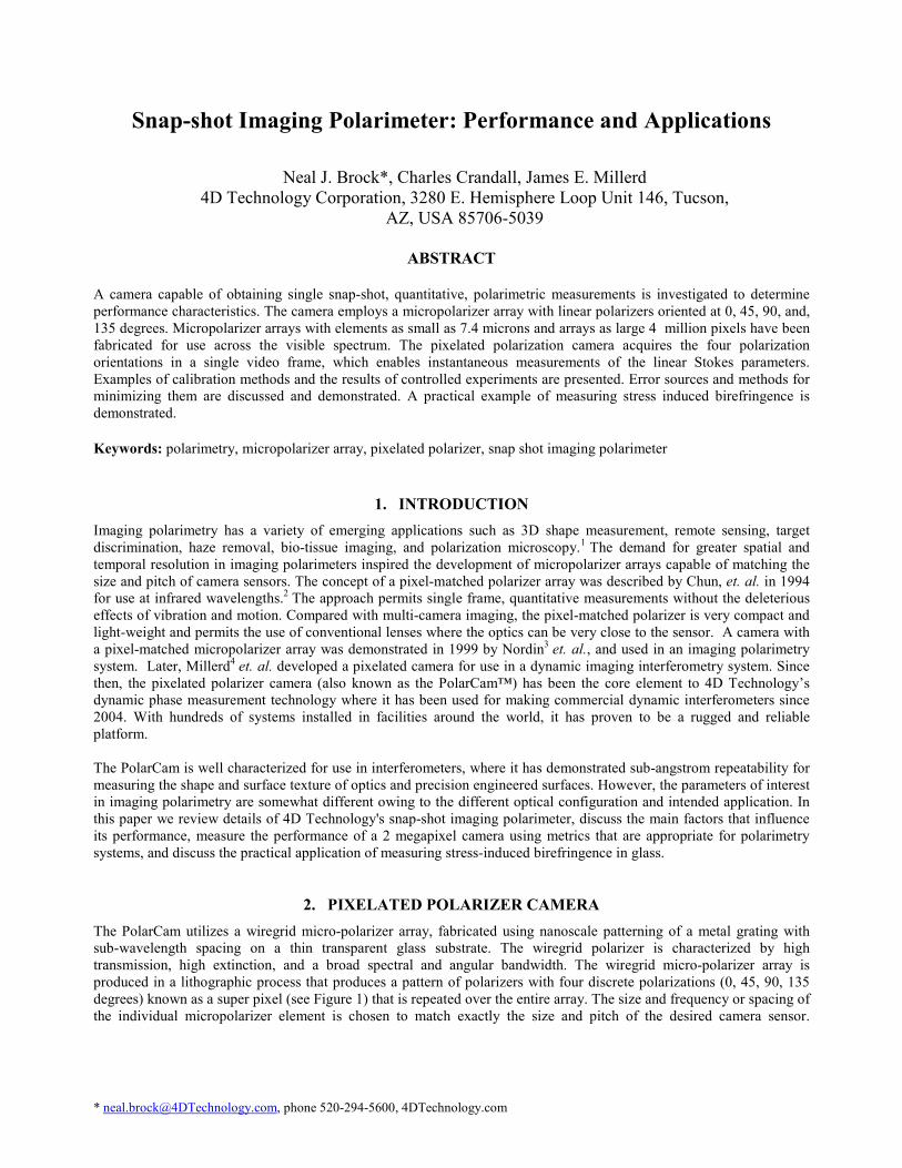
Figure 12 shows an optical arrangement that was used to measure birefringence in a thin glass sample. The light is

generated from an LED source and polarized circularly using a combination of a linear polarizer and a quarter-wave

retardation plate. The light was then transmitted through a homogeneous, transparent glass disk that was mounted with

three contact pads spaced by 120 degrees around the diameter of the glass. One of the pads could be adjusted to produce

variable stress.

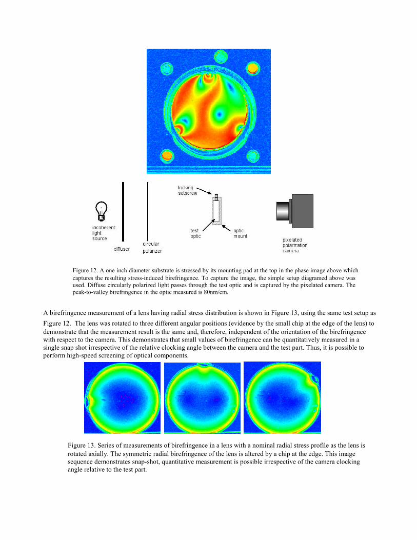
A birefringence measurement of a lens having radial stress distribution is shown in Figure 13, using the same test setup as

Figure 12. The lens was rotated to three different angular positions (evidence by the small chip at the edge of the lens) to

demonstrate that the measurement result is the same and, therefore, independent of the orientation of the birefringence

with respect to the camera. This demonstrates that small values of birefringence can be quantitatively measured in a

single snap shot irrespective of the relative clocking angle between the camera and the test part. Thus, it is possible to

perform high-speed screening of optical components.

Figure 13. Series of measurements of birefringence in a lens with a nominal radial stress profile as the lens is

rotated axially. The symmetric radial birefringence of the lens is altered by a chip at the edge. This image

sequence demonstrates snap-shot, quantitative measurement is possible irrespective of the camera clocking

angle relative to the test part.

Figure 12. A one inch diameter substrate is stressed by its mounting pad at the top in the phase image above which

captures the resulting stress-induced birefringence. To capture the image, the simple setup diagramed above was

used. Diffuse circularly polarized light passes through the test optic and is captured by the pixelated camera. The

peak-to-valley birefringence in the optic measured is 80nm/cm.

7. CONCLUSIONS

The use of a solid state micropolarizer camera permits single shot acquisition of polarimetric data that can freeze out

motion and vibration, and enables high frame rate acquisition. Compared with multi-camera imaging systems, the

pixelated camera approach is extremely compact and permits the use of high NA imaging systems with minimal

requirements on clearance between the optics and the sensor. Novel processing algorithms can be used to achieve a

spatial frequency response from the sensor that is nearly equal to the limit imposed by the finite pixel width. Care must

be taken to optimize the optical imaging system and the camera parameters to minimize crosstalk and maximize

measurement dynamic range. Measurements of AoLP show single shot measurement resolution in the range of +/-0.25

degrees, while DoLP shows +/-2.5%. Both of these can be improved substantially with temporal averaging at the

expense of measurement time. However, this resolution is adequate for many applications such as birefringence

measurement in optical glass where it is possible to measure a retardance range of 125nm with a noise floor of 2.5nm.

REFERENCES

[1] Tyo, J. S., Goldstein, D. L., Chenault, D. B., and Shaw, J. A., “Review of passive imaging polarimetry for remote

sensing applications,” Applied Optics, 45 (22), 5453-5469 (2006).

[2] Chun, C. S. L., Fleming, D. L., Torok, E., J., “Polarization sensitive, thermal imaging,” SPIE 2234, 275-286 (1994).

[3] Nordin, G. P., Meier, J. T., Deguzman, P. C., and Jones, M. W., “Micropolarizer array for infrared imaging

polarimetry,” J. Opt. Soc. Am A, 16(5), (1999).

[4] Millerd, J. E., Brock, N. J., Hayes, J. B., North-Morris, M., Novak, M., and, Wyant, J. C., “Pixelated phase-mask

dynamic interferometer,” Proc. SPIE 5531, 304-315 (2004).

[5] Kimbrough, B.T., “Pixelated mask spatial carrier phase shifting interferometry algorithms and associated errors,”

Applied Optics 45(19), 4554–4562 (2006).

[6] Jones, M. W., Persons, C. M., “Performance predictions for micropolarizer array imaging polarimeters,” Proc. SPIE

6682, 1-11 (2007).

[7 ] Moxtek Inc. Data Sheet: OPT-DATA-1005, Rev B.

[8] William Shurcliff, Polarized Light Production and Use, Harvard University Press, 1962.

[9] Tyo, J. S., LaCasse, C. F., and Ratliff, B. M., “Total elimination of sampling errors in polarization imager obtained

with integrated microgrid polarimeters,” Optics Letters 34(20), 3187–3189 (2009).