snapshot ensembles: train 1, get m for free

Published as a conference paper at ICLR 2017

SNAPSHOT ENSEMBLES: TRAIN 1, GET M FOR FREE

Gao Huang∗, Yixuan Li∗, Geoff PleissCornell University{gh349, yl2363}@cornell.edu, [email protected]

Zhuang LiuTsinghua [email protected]

John E. Hopcroft, Kilian Q. WeinbergerCornell [email protected], [email protected]

ABSTRACT

Ensembles of neural networks are known to be much more robust and accuratethan individual networks. However, training multiple deep networks for modelaveraging is computationally expensive. In this paper, we propose a method toobtain the seemingly contradictory goal of ensembling multiple neural networksat no additional training cost. We achieve this goal by training a single neural net-work, converging to several local minima along its optimization path and savingthe model parameters. To obtain repeated rapid convergence, we leverage recentwork on cyclic learning rate schedules. The resulting technique, which we refer toas Snapshot Ensembling, is simple, yet surprisingly effective. We show in a seriesof experiments that our approach is compatible with diverse network architecturesand learning tasks. It consistently yields lower error rates than state-of-the-artsingle models at no additional training cost, and compares favorably with tradi-tional network ensembles. On CIFAR-10 and CIFAR-100 our DenseNet SnapshotEnsembles obtain error rates of 3.4% and 17.4% respectively.

1 INTRODUCTION

Stochastic Gradient Descent (SGD) (Bottou, 2010) and its accelerated variants (Kingma & Ba, 2014;Duchi et al., 2011) have become the de-facto approaches for optimizing deep neural networks. Thepopularity of SGD can be attributed to its ability to avoid and even escape spurious saddle-pointsand local minima (Dauphin et al., 2014). Although avoiding these spurious solutions is generallyconsidered positive, in this paper we argue that these local minima contain useful information thatmay in fact improve model performance.

Although deep networks typically never converge to a global minimum, there is a notion of “good”and “bad” local minima with respect to generalization. Keskar et al. (2016) argue that local minimawith flat basins tend to generalize better. SGD tends to avoid sharper local minima because gradientsare computed from small mini-batches and are therefore inexact (Keskar et al., 2016). If the learning-rate is sufficiently large, the intrinsic random motion across gradient steps prevents the optimizerfrom reaching any of the sharp basins along its optimization path. However, if the learning rateis small, the model tends to converge into the closest local minimum. These two very differentbehaviors of SGD are typically exploited in different phases of optimization (He et al., 2016a).Initially the learning rate is kept high to move into the general vicinity of a flat local minimum. Oncethis search has reached a stage in which no further progress is made, the learning rate is dropped(once or twice), triggering a descent, and ultimately convergence, to the final local minimum.

It is well established (Kawaguchi, 2016) that the number of possible local minima grows expo-nentially with the number of parameters—of which modern neural networks can have millions. Itis therefore not surprising that two identical architectures optimized with different initializations orminibatch orderings will converge to different solutions. Although different local minima often havevery similar error rates, the corresponding neural networks tend to make different mistakes. This

∗Authors contribute equally.

1


010

2030

4050

010

2030

4050

−0.4

−0.3

−0.2

−0.1

0

0.1

0.2

0.3

0.4

0.5 Single ModelStandard LR Schedule

010

2030

4050

010

2030

4050

−0.4

−0.3

−0.2

−0.1

0

0.1

0.2

0.3

0.4

0.5

3

12

Snapshot EnsembleCyclic LR Schedule

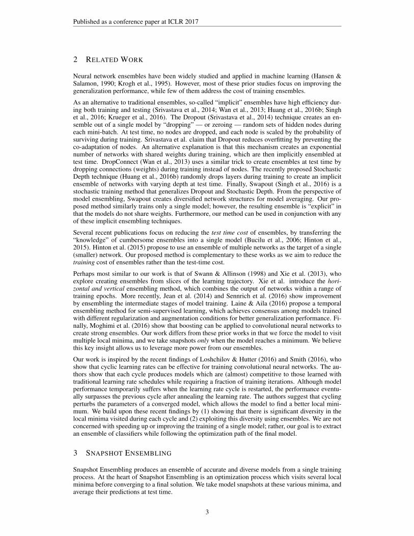
Figure 1: Left: Illustration of SGD optimization with a typical learning rate schedule. The model convergesto a minimum at the end of training. Right: Illustration of Snapshot Ensembling. The model undergoes severallearning rate annealing cycles, converging to and escaping from multiple local minima. We take a snapshot ateach minimum for test-time ensembling.

diversity can be exploited through ensembling, in which multiple neural networks are trained fromdifferent initializations and then combined with majority voting or averaging (Caruana et al., 2004).Ensembling often leads to drastic reductions in error rates. In fact, most high profile competitions,e.g. Imagenet (Deng et al., 2009) or Kaggle1, are won by ensembles of deep learning architectures.

Despite its obvious advantages, the use of ensembling for deep networks is not nearly as wide-spread as it is for other algorithms. One likely reason for this lack of adaptation may be the costof learning multiple neural networks. Training deep networks can last for weeks, even on highperformance hardware with GPU acceleration. As the training cost for ensembles increases linearly,ensembles can quickly becomes uneconomical for most researchers without access to industrialscale computational resources.

In this paper we focus on the seemingly-contradictory goal of learning an ensemble of multipleneural networks without incurring any additional training costs. We achieve this goal with a trainingmethod that is simple and straight-forward to implement. Our approach leverages the non-convexnature of neural networks and the ability of SGD to converge to and escape from local minima ondemand. Instead of training M neural networks independently from scratch, we let SGD convergeM times to local minima along its optimization path. Each time the model converges, we save theweights and add the corresponding network to our ensemble. We then restart the optimization witha large learning rate to escape the current local minimum. More specifically, we adopt the cyclingprocedure suggested by Loshchilov & Hutter (2016), in which the learning rate is abruptly raised andthen quickly lowered to follow a cosine function. Because our final ensemble consists of snapshotsof the optimization path, we refer to our approach as Snapshot Ensembling. Figure 1 presents ahigh-level overview of this method.

In contrast to traditional ensembles, the training time for the entire ensemble is identical to the timerequired to train a single traditional model. During testing time, one can evaluate and average thelast (and therefore most accurate) m out of M models. Our approach is naturally compatible withother methods to improve the accuracy, such as data augmentation, stochastic depth (Huang et al.,2016b), or batch normalization (Ioffe & Szegedy, 2015). In fact, Snapshot Ensembles can even beensembled, if for example parallel resources are available during training. In this case, an ensembleof K Snapshot Ensembles yields K ×M models at K times the training cost.

We evaluate the efficacy of Snapshot Ensembles on three state-of-the-art deep learning architecturesfor object recognition: ResNet (He et al., 2016b), Wide-ResNet (Zagoruyko & Komodakis, 2016),and DenseNet (Huang et al., 2016a). We show across four different data sets that Snapshot Ensem-bles almost always reduce error without increasing training costs. For example, on CIFAR-10 andCIFAR-100, Snapshot Ensembles obtains error rates of 3.44% and 17.41% respectively.

1www.kaggle.com

2

www.kaggle.com


2 RELATED WORK

Neural network ensembles have been widely studied and applied in machine learning (Hansen &Salamon, 1990; Krogh et al., 1995). However, most of these prior studies focus on improving thegeneralization performance, while few of them address the cost of training ensembles.

As an alternative to traditional ensembles, so-called “implicit” ensembles have high efficiency dur-ing both training and testing (Srivastava et al., 2014; Wan et al., 2013; Huang et al., 2016b; Singhet al., 2016; Krueger et al., 2016). The Dropout (Srivastava et al., 2014) technique creates an en-semble out of a single model by “dropping” — or zeroing — random sets of hidden nodes duringeach mini-batch. At test time, no nodes are dropped, and each node is scaled by the probability ofsurviving during training. Srivastava et al. claim that Dropout reduces overfitting by preventing theco-adaptation of nodes. An alternative explanation is that this mechanism creates an exponentialnumber of networks with shared weights during training, which are then implicitly ensembled attest time. DropConnect (Wan et al., 2013) uses a similar trick to create ensembles at test time bydropping connections (weights) during training instead of nodes. The recently proposed StochasticDepth technique (Huang et al., 2016b) randomly drops layers during training to create an implicitensemble of networks with varying depth at test time. Finally, Swapout (Singh et al., 2016) is astochastic training method that generalizes Dropout and Stochastic Depth. From the perspective ofmodel ensembling, Swapout creates diversified network structures for model averaging. Our pro-posed method similarly trains only a single model; however, the resulting ensemble is “explicit” inthat the models do not share weights. Furthermore, our method can be used in conjunction with anyof these implicit ensembling techniques.

Several recent publications focus on reducing the test time cost of ensembles, by transferring the“knowledge” of cumbersome ensembles into a single model (Bucilu et al., 2006; Hinton et al.,2015). Hinton et al. (2015) propose to use an ensemble of multiple networks as the target of a single(smaller) network. Our proposed method is complementary to these works as we aim to reduce thetraining cost of ensembles rather than the test-time cost.

Perhaps most similar to our work is that of Swann & Allinson (1998) and Xie et al. (2013), whoexplore creating ensembles from slices of the learning trajectory. Xie et al. introduce the hori-zontal and vertical ensembling method, which combines the output of networks within a range oftraining epochs. More recently, Jean et al. (2014) and Sennrich et al. (2016) show improvementby ensembling the intermediate stages of model training. Laine & Aila (2016) propose a temporalensembling method for semi-supervised learning, which achieves consensus among models trainedwith different regularization and augmentation conditions for better generalization performance. Fi-nally, Moghimi et al. (2016) show that boosting can be applied to convolutional neural networks tocreate strong ensembles. Our work differs from these prior works in that we force the model to visitmultiple local minima, and we take snapshots only when the model reaches a minimum. We believethis key insight allows us to leverage more power from our ensembles.

Our work is inspired by the recent findings of Loshchilov & Hutter (2016) and Smith (2016), whoshow that cyclic learning rates can be effective for training convolutional neural networks. The au-thors show that each cycle produces models which are (almost) competitive to those learned withtraditional learning rate schedules while requiring a fraction of training iterations. Although modelperformance temporarily suffers when the learning rate cycle is restarted, the performance eventu-ally surpasses the previous cycle after annealing the learning rate. The authors suggest that cyclingperturbs the parameters of a converged model, which allows the model to find a better local mini-mum. We build upon these recent findings by (1) showing that there is significant diversity in thelocal minima visited during each cycle and (2) exploiting this diversity using ensembles. We are notconcerned with speeding up or improving the training of a single model; rather, our goal is to extractan ensemble of classifiers while following the optimization path of the final model.

3 SNAPSHOT ENSEMBLING

Snapshot Ensembling produces an ensemble of accurate and diverse models from a single trainingprocess. At the heart of Snapshot Ensembling is an optimization process which visits several localminima before converging to a final solution. We take model snapshots at these various minima, andaverage their predictions at test time.

3


Ensembles work best if the individual models (1) have low test error and (2) do not overlap in theset of examples they misclassify. Along most of the optimization path, the weight assignments ofa neural network tend not to correspond to low test error. In fact, it is commonly observed that thevalidation error drops significantly only after the learning rate has been reduced, which is typicallydone after several hundred epochs. Our approach is inspired by the observation that training neuralnetworks for fewer epochs and dropping the learning rate earlier has minor impact on the final testerror (Loshchilov & Hutter, 2016). This seems to suggest that local minima along the optimizationpath become promising (in terms of generalization error) after only a few epochs.

Model 1

Model 2

Model 3

Model 4

Model 5

Model 6

Figure 2: Training loss of 100-layer DenseNet on CI-FAR10 using standard learning rate (blue) and M = 6cosine annealing cycles (red). The intermediate mod-els, denoted by the dotted lines, form an ensemble atthe end of training.

Cyclic Cosine Annealing. To converge to mul-tiple local minima, we follow a cyclic annealingschedule as proposed by Loshchilov & Hutter(2016). We lower the learning rate at a veryfast pace, encouraging the model to convergetowards its first local minimum after as few as50 epochs. The optimization is then contin-ued at a larger learning rate, which perturbs themodel and dislodges it from the minimum. Werepeat this process several times to obtain mul-tiple convergences. Formally, the learning rateα has the form:

α(t) = f (mod (t− 1, dT/Me)) , (1)

where t is the iteration number, T is the to-tal number of training iterations, and f is amonotonically decreasing function. In otherwords, we split the training process into M cy-cles, each of which starts with a large learningrate, which is annealed to a smaller learningrate. The large learning rate α = f(0) pro-vides the model enough energy to escape froma critical point, while the small learning rateα = f(dT/Me) drives the model to a well behaved local minimum. In our experiments, we setf to be the shifted cosine function proposed by Loshchilov & Hutter (2016):

α(t) =α0

2

(cos

(πmod(t− 1, dT/Me)

dT/Me

)+ 1

), (2)

where α0 is the initial learning rate. Intuitively, this function anneals the learning rate from its initialvalue α0 to f(dT/Me) ≈ 0 over the course of a cycle. Following (Loshchilov & Hutter, 2016), weupdate the learning rate at each iteration rather than at every epoch. This improves the convergenceof short cycles, even when a large initial learning rate is used.Snapshot Ensembling. Figure 2 depicts the training process using cyclic and traditional learningrate schedules. At the end of each training cycle, it is apparent that the model reaches a local mini-mum with respect to the training loss. Thus, before raising the learning rate, we take a “snapshot”of the model weights (indicated as vertical dashed black lines). After training M cycles, we haveM model snapshots, f1 . . . fM , each of which will be used in the final ensemble. It is important tohighlight that the total training time of the M snapshots is the same as training a model with a stan-dard schedule (indicated in blue). In some cases, the standard learning rate schedule achieves lowertraining loss than the cyclic schedule; however, as we will show in the next section, the benefits ofensembling outweigh this difference.Ensembling at Test Time. The ensemble prediction at test time is the average of the last m(m ≤ M ) model’s softmax outputs. Let x be a test sample and let hi (x) be the softmaxscore of snapshot i. The output of the ensemble is a simple average of the last m models:hEnsemble = 1

m

∑m−10 hM−i (x) . We always ensemble the last m models, as these models tend

to have the lowest test error.

4


Method C10 C100 SVHN Tiny ImageNet

ResNet-110

Single model 5.52 28.02 1.96 46.50NoCycle Snapshot Ensemble 5.49 26.97 1.78 43.69

SingleCycle Ensembles 6.66 24.54 1.74 42.60Snapshot Ensemble (α0 = 0.1) 5.73 25.55 1.63 40.54Snapshot Ensemble (α0 = 0.2) 5.32 24.19 1.66 39.40

Wide-ResNet-32

Single model 5.43 23.55 1.90 39.63Dropout 4.68 22.82 1.81 36.58

NoCycle Snapshot Ensemble 5.18 22.81 1.81 38.64SingleCycle Ensembles 5.95 21.38 1.65 35.53

Snapshot Ensemble (α0 = 0.1) 4.41 21.26 1.64 35.45Snapshot Ensemble (α0 = 0.2) 4.73 21.56 1.51 32.90

DenseNet-40

Single model 5.24∗ 24.42∗ 1.77 39.09Dropout 6.08 25.79 1.79∗ 39.68

NoCycle Snapshot Ensemble 5.20 24.63 1.80 38.51SingleCycle Ensembles 5.43 22.51 1.87 38.00

Snapshot Ensemble (α0 = 0.1) 4.99 23.34 1.64 37.25Snapshot Ensemble (α0 = 0.2) 4.84 21.93 1.73 36.61

DenseNet-100

Single model 3.74∗ 19.25∗ - -Dropout 3.65 18.77 - -

NoCycle Snapshot Ensemble 3.80 19.30 - -SingleCycle Ensembles 4.52 18.38

Snapshot Ensemble (α0 = 0.1) 3.57 18.12 - -Snapshot Ensemble (α0 = 0.2) 3.44 17.41 - -

Table 1: Error rates (%) on CIFAR-10 and CIFAR-100 datasets. All methods in the same group are trainedfor the same number of iterations. Results of our method are colored in blue, and the best result for eachnetwork/dataset pair are bolded. ∗ indicates numbers which we take directly from Huang et al. (2016a).

4 EXPERIMENTS

We demonstrate the effectiveness of Snapshot Ensembles on several benchmark datasets, comparingwith competitive baselines. We run all experiments with Torch 7 (Collobert et al., 2011)2.

4.1 DATASETS

CIFAR. The two CIFAR datasets (Krizhevsky & Hinton, 2009) consist of colored natural imagessized at 32×32 pixels. CIFAR-10 (C10) and CIFAR-100 (C100) images are drawn from 10 and 100classes, respectively. For each dataset, there are 50,000 training images and 10,000 images reservedfor testing. We use a standard data augmentation scheme (Lin et al., 2013; Romero et al., 2014; Leeet al., 2015; Springenberg et al., 2014; Srivastava et al., 2015; Huang et al., 2016b; Larsson et al.,2016), in which the images are zero-padded with 4 pixels on each side, randomly cropped to produce32×32 images, and horizontally mirrored with probability 0.5.SVHN. The Street View House Numbers (SVHN) dataset (Netzer et al., 2011) contains 32 × 32colored digit images from Google Street View, with one class for each digit. There are 73,257images in the training set and 26,032 images in the test set. Following common practice (Sermanetet al., 2012; Goodfellow et al., 2013; Huang et al., 2016a), we withhold 6,000 training images forvalidation, and train on the remaining images without data augmentation.Tiny ImageNet. The Tiny ImageNet dataset3 consists of a subset of ImageNet images (Deng et al.,2009). There are 200 classes, each of which has 500 training images and 50 validation images.Each image is resized to 64×64 and augmented with random crops, horizontal mirroring, and RGBintensity scaling (Krizhevsky et al., 2012).ImageNet. The ILSVRC 2012 classification dataset (Deng et al., 2009) consists of 1000 imagesclasses, with a total of 1.2 million training images and 50,000 validation images. We adopt the same

2Code to reproduce results is available at https://github.com/gaohuang/SnapshotEnsemble3https://tiny-imagenet.herokuapp.com

5

https://github.com/gaohuang/SnapshotEnsemble

https://tiny-imagenet.herokuapp.com


1 2 3 4 5 6

# of snapshots

3.4

3.5

3.6

3.7

3.8

3.9

4.0

4.1

Test

Err

or

(%)

Cifar10 (α0 = 0. 1)

DenseNet Baseline(Huang et al. 2016)

1 2 3 4 5 6

# of snapshots

17.0

17.5

18.0

18.5

19.0

19.5

20.0

20.5Cifar100 (α0 = 0. 1)


1 2 3 4 5 6

# of snapshots

3.4

3.5

3.6

3.7

3.8

3.9

4.0

4.1

Test

Err

or

(%)

Cifar10 (α0 = 0. 2)


1 2 3 4 5 6

# of snapshots

17.0

17.5

18.0

18.5

19.0

19.5

20.0

20.5Cifar100 (α0 = 0. 2)


Figure 3: DenseNet-100 Snapshot Ensemble performance on CIFAR-10 and CIFAR-100 with restart learningrate α0 = 0.1 (left two) and α0 = 0.2 (right two). Each ensemble is trained with M =6 annealing cycles (50epochs per each).

data augmentation scheme as in (He et al., 2016a; Huang et al., 2016a) and apply a 224×224 centercrop to images at test time.

4.2 TRAINING SETTING

Architectures. We test several state-of-the-art architectures, including residual networks(ResNet) (He et al., 2016a), Wide ResNet (Zagoruyko & Komodakis, 2016) and DenseNet (Huanget al., 2016a). For ResNet, we use the original 110-layer network introduced by He et al. (2016a).Wide-ResNet is a 32-layer ResNet with 4 times as many convolutional features per layer as a stan-dard ResNet. For DenseNet, our large model follows the same setup as (Huang et al., 2016a),with depth L = 100 and growth rate k = 24. In addition, we also evaluate our method on a smallDenseNet, with depth L = 40 and k = 12. To adapt all these networks to Tiny ImageNet, we add astride of 2 to the first layer of the models, which downsamples the images to 32×32. For ImageNet,we test the 50-layer ResNet proposed in (He et al., 2016a). We use a mini batch size of 64.4

Baselines. Snapshot Ensembles incur the training cost of a single model; therefore, we comparewith baselines that require the same amount of training. First, we compare against a Single Modeltrained with a standard learning rate schedule, dropping the learning rate from 0.1 to 0.01 halfwaythrough training, and then to 0.001 when training is at 75%. Additionally, to compare againstimplicit ensembling methods, we test against a single model trained with Dropout. This baselineuses the same learning rate as above, and drops nodes during training with a probability of 0.2.

We then test the Snapshot Ensemble algorithm trained with the cyclic cosine learning rate as de-scribed in (2). We test models with the max learning rate α0 set to 0.1 and 0.2. In both cases, wedivide the training process into learning rate cycles. Model snapshots are taken after each learn-ing rate cycle. Additionally, we train a Snapshot Ensemble with a non-cyclic learning rate schedule.This NoCycle Snapshot Ensemble, which uses the same schedule as the Single Model and Dropoutbaselines, is meant to highlight the impact of cyclic learning rates for our method. To accuratelycompare with the cyclic Snapshot Ensembles, we take the same number of snapshots equally spacedthroughout the training process. Finally, we compare against SingleCycle Ensembles, a SnapshotEnsemble variant in which the network is re-initialized at the beginning of every cosine learningrate cycle, rather than using the parameters from the previous optimization cycle. This baseline es-sentially creates a traditional ensemble, yet each network only has 1/M of the typical training time.This variant is meant to highlight the tradeoff between model diversity and model convergence.Though SingleCycle Ensembles should in theory explore more of the parameter space, the modelsdo not benefit from the optimization of previous cycles.Training Budget. On CIFAR datasets, the training budget is B = 300 epochs for DenseNet-40 andDenseNet-100, and B = 200 for ResNet and Wide ResNet models. Snapshot variants are trainedwith M = 6 cycles of B/M = 50 epochs for DenseNets, and M = 5 cycles of B/M = 40 epochsfor ResNets/Wide ResNets. SVHN models are trained with a budget of B = 40 epochs (5 cyclesof 8 epochs). For Tiny ImageNet, we use a training budget of B = 150 (6 cycles of 25 epochs).Finally, ImageNet is trained with a budget of B = 90 epochs, and we trained 2 Snapshot variants:one with M = 2 cycles and one with M = 3.

4Exceptions: ResNet-110 and Wide-ResNet are trained with batch size 128 on Tiny ImageNet. The Ima-geNet model is trained with batch size 256.

6


4.3 SNAPSHOT ENSEMBLE RESULTS

Method Val. Error (%)

Single model 24.01Snapshot Ensemble (M = 2) 23.33Snapshot Ensemble (M = 3) 23.96

Table 2: Top-1 error rates (%) on ImageNet validationset using ResNet-50 with varying number of cycles.

Accuracy. The main results are summarizedin Table 1. In most cases, Snapshot ensem-bles achieve lower error than any of the base-line methods. Most notably, Snapshot Ensem-bles yield an error rate of 17.41% on CIFAR-100 using large DenseNets, far outperformingthe record of 19.25% under the same trainingcost and architecture (Huang et al., 2016a). Ourmethod has the most success on CIFAR-100and Tiny ImageNet, which is likely due to thecomplexity of these datasets. The softmax outputs for these datasets are high dimensional due to thelarge number of classes, making it unlikely that any two models make the same predictions. Snap-shot Ensembling is also capable of improving the competitive baselines for CIFAR-10 and SVHNas well, reducing error by 1% and 0.4% respectively with the Wide ResNet architecture.

The NoCycle Snapshot Ensemble generally has little effect on performance, and in some instanceseven increases the test error. This highlights the need for a cyclic learning rate for useful ensembling.The SingleCycle Ensemble has similarly mixed performance. In some cases, e.g., DenseNet-40 onCIFAR-100, the SingleCycle Ensemble is competitive with Snapshot Ensembles. However, as themodel size increases to 100 layers, it does not perform as well. This is because it is difficult to train alarge model from scratch in only a few epochs. These results demonstrate that Snapshot Ensemblestend to work best when utilizing information from previous cycles. Effectively, Snapshot Ensemblesstrike a balance between model diversity and optimization.

Table 2 shows Snapshot Ensemble results on ImageNet. The Snapshot Ensemble with M = 2achieves 23.33% validation error, outperforming the single model baseline with 24.01% validationerror. It appears that 2 cycles is the optimal choice for the ImageNet dataset. Provided with thelimited total training budget B = 90 epochs, we hypothesize that allocating fewer than B/2 = 45epochs per training cycle is insufficient for the model to converge on such a large dataset.

M Test Error (%)

2 22.924 22.076 21.938 21.8910 22.16

Table 3: Error rates ofa DenseNet-40 SnapshotEnsemble on CIFAR-100,varying M—the number ofmodels (cycles) used in theensemble.

Ensemble Size. In some applications, it may be beneficial to vary thesize of the ensemble dynamically at test time depending on availableresources. Figure 3 displays the performance of DenseNet-40 on theCIFAR-100 dataset as the effective ensemble size,m, is varied. Each en-semble consists of snapshots from later cycles, as these snapshots havereceived the most training and therefore have likely converged to bet-ter minima. Although ensembling more models generally gives betterperformance, we observe significant drops in error when the second andthird models are added to the ensemble. In most cases, an ensemble oftwo models outperforms the baseline model.Restart Learning Rate. The effect of the restart learning rate can beobserved in Figure 3. The left two plots show performance when usinga restart learning rate of α0 = 0.1 at the beginning of each cycle, andthe right two plots show α0 = 0.2. In most cases, ensembles with thelarger restart learning rate perform better, presumably because the strongperturbation in between cycles increases the diversity of local minima.Varying Number of Cycles. Given a fixed training budget, there is a trade-off between the numberof learning rate cycles and their length. Therefore, we investigate how the number of cycles Maffects the ensemble performance, given a fixed training budget. We train a 40-layer DenseNet onthe CIFAR-100 dataset with an initial learning rate of α0 = 0.2. We fix the total training budgetB = 300 epochs, and vary the value of M ∈ {2, 4, 6, 8, 10}. As shown in Table 3, our method isrelatively robust with respect to different values of M . At the extremes, M = 2 and M = 10, wefind a slight degradation in performance, as the cycles are either too few or too short. In practice, wefind that setting M to be 4 ∼ 8 works reasonably well.Varying Training Budget. The left and middle panels of Figure 4 show the performance of Snap-shot Ensembles and SingleCycle Ensembles as a function of training budget (where the number ofcycles is fixed at M = 6). We train a 40-layer DenseNet on CIFAR-10 and CIFAR-100, with an ini-tial learning rate of α0 = 0.1, varying the total number of training epochs from 60 to 300. We observe

7


100 150 200 250 300

Training budget B (epochs)

4

5

6

7

8

9

10

11

En

sem

ble

Test

Err

or

(%)

Cifar10, DenseNet-40

Snapshot Ensemble

SingleCycle Ensemble

100 150 200 250 300

Training budget B (epochs)

22

24

26

28

30

32

34

36

38

En

sem

ble

Test

Err

or

(%)


Snapshot Ensemble

SingleCycle Ensemble

1 2 3 4 5 6

# of models

14

16

18

20

22

24

26

28

En

sem

ble

Test

Err

or

(%)


Single Model

Snapshot ensemble(50 epochs per model cost)

True ensemble of fully trained models(300 epochs per model cost)

Figure 4: Snapshot Ensembles under different training budgets on (Left) CIFAR-10 and (Middle) CIFAR-100.Right: Comparison of Snapshot Ensembles with true ensembles.

Figure 5: Interpolations in parameter space between the final model (sixth snapshot) and all intermediatesnapshots. λ = 0 represents an intermediate snapshot model, while λ = 1 represents the final model. Left: ASnapshot Ensemble, with cosine annealing cycles (α0 = 0.2 every B/M = 50 epochs). Right: A NoCycleSnapshot Ensemble, (two learning rate drops, snapshots every 50 epochs).

that both Snapshot Ensembles and SingleCycle Ensembles become more accurate as training bud-get increases. However, we note that as training budget decreases, Snapshot Ensembles still yieldcompetitive results, while the performance of the SingleCycle Ensembles degrades rapidly. Theseresults highlight the improvements that Snapshot Ensembles obtain when the budget is low. If thebudget is high, then the SingleCycle baseline approaches true ensembles and outperforms Snapshotensembles eventually.Comparison with True Ensembles. We compare Snapshot Ensembles with the traditional ensem-bling method. The right panel of Figure 4 shows the test error rates of DenseNet-40 on CIFAR-100.The true ensemble method averages models that are trained with 300 full epochs, each with differ-ent weight initializations. Given the same number of models at test time, the error rate of the trueensemble can be seen as a lower bound of our method. Our method achieves performance that iscomparable with ensembling of 2 independent models, but with the training cost of one model.

4.4 DIVERSITY OF MODEL ENSEMBLES

Parameter Space. We hypothesize that the cyclic learning rate schedule creates snapshots which arenot only accurate but also diverse with respect to model predictions. We qualitatively measure thisdiversity by visualizing the local minima that models converge to. To do so, we linearly interpolatesnapshot models, as described by Goodfellow et al. (2014). Let J (θ) be the test error of a modelusing parameters θ. Given θ1 and θ2 — the parameters from models 1 and 2 respectively — we cancompute the loss for a convex combination of model parameters: J (λ (θ1) + (1− λ) (θ2)), where λis a mixing coefficient. Setting λ to 1 results in a parameters that are entirely θ1 while setting λ to 0gives the parameters θ2. By sweeping the values of λ, we can examine a linear slice of the parameterspace. Two models that converge to a similar minimum will have smooth parameter interpolations,whereas models that converge to different minima will likely have a non-convex interpolation, witha spike in error when λ is between 0 and 1.

Figure 5 displays interpolations between the final model of DenseNet-40 (sixth snapshot) and allintermediate snapshots. The left two plots show Snapshot Ensemble models trained with a cycliclearning rate, while the right two plots show NoCycle Snapshot models. λ = 0 represents a modelwhich is entirely snapshot parameters, while λ = 1 represents a model which is entirely the param-eters of the final model. From this figure, it is clear that there are differences between cyclic and

8


non-cyclic learning rate schedules. Firstly, all of the cyclic snapshots achieve roughly the same erroras the final cyclical model, as the error is similar for λ = 0 and λ = 1. Additionally, it appearsthat most snapshots do not lie in the same minimum as the final model. Thus the snapshots arelikely to misclassify different samples. Conversely, the first three snapshots achieve much highererror than the final model. This can be observed by the sharp minima around λ = 1, which suggeststhat mixing in any amount of the snapshot parameters will worsen performance. While the finaltwo snapshots achieve low error, the figures suggests that they lie in the same minimum as the finalmodel, and therefore likely add limited diversity to the ensemble.

1 2 3 4 5 6

65

43

21

0.88 0.9 0.91 0.92 0.93 1

0.88 0.91 0.92 0.93 1 0.93

0.88 0.91 0.93 1 0.93 0.92

0.89 0.92 1 0.93 0.92 0.91

0.9 1 0.92 0.91 0.91 0.9

1 0.9 0.89 0.88 0.88 0.88

Cosine with restart (CIFAR100)

1 2 3 4 5 6

65

43

21

0.82 0.83 0.84 0.99 0.99 1

0.82 0.83 0.84 0.99 1 0.99

0.82 0.83 0.84 1 0.99 0.99

0.76 0.78 1 0.84 0.84 0.84

0.78 1 0.78 0.83 0.83 0.83

1 0.78 0.76 0.82 0.82 0.82

Standard lr scheduling (CIFAR100)

Figure 6: Pairwise correlation of softmax outputs be-tween any two snapshots for DenseNet-100. Left:A Snapshot Ensemble, with cosine annealing cycles(restart with α0 = 0.2 every 50 epochs). Right: ANoCycle Snapshot Ensemble, (two learning rate drops,snapshots every 50 epochs).

Activation space. To further explore the diver-sity of models, we compute the pairwise corre-lation of softmax outputs for every pair of snap-shots. Figure 6 displays the average correla-tion for both cyclic snapshots and non-cyclicalsnapshots. Firstly, there are large correlationsbetween the last 3 snapshots of the non-cyclictraining schedule (right). These snapshots aretaken after dropping the learning rate, suggest-ing that each snapshot has converged to thesame minimum. Though there is more diversityamongst the earlier snapshots, these snapshotshave much higher error rates and are thereforenot ideal for ensembling. Conversely, thereis less correlation between all cyclic snapshots(left). Because all snapshots have similar accu-racy (as can be seen in Figure 5), these differ-ences in predictions can be exploited to createeffective ensembles.

5 DISCUSSION

We introduce Snapshot Ensembling, a simple method to obtain ensembles of neural networks with-out any additional training cost. Our method exploits the ability of SGD to converge to and escapefrom local minima as the learning rate is lowered, which allows the model to visit several weightassignments that lead to increasingly accurate predictions over the course of training. We harnessthis power with the cyclical learning rate schedule proposed by Loshchilov & Hutter (2016), savingmodel snapshots at each point of convergence. We show in several experiments that all snapshotsare accurate, yet produce different predictions from one another, and therefore are well suited fortest-time ensembles. Ensembles of these snapshots significantly improve the state-of-the-art onCIFAR-10, CIFAR-100 and SVHN. Future work will explore combining Snapshot Ensembles withtraditional ensembles. In particular, we will investigate how to balance growing an ensemble withnew models (with random initializations) and refining existing models with further training cyclesunder a fixed training budget.

ACKNOWLEDGEMENTS

We thank Ilya Loshchilov and Frank Hutter for their insightful comments on the cyclic cosine-shaped learning rate. The authors are supported in part by the, III-1618134, III-1526012, IIS-1149882 grants from the National Science Foundation, US Army Research Office W911NF-14-1-0477, and the Bill and Melinda Gates Foundation.

REFERENCES

Leon Bottou. Large-scale machine learning with stochastic gradient descent. In COMPSTAT. 2010.

Cristian Bucilu, Rich Caruana, and Alexandru Niculescu-Mizil. Model compression. In KDD, 2006.

Rich Caruana, Alexandru Niculescu-Mizil, Geoff Crew, and Alex Ksikes. Ensemble selection fromlibraries of models. In ICML, 2004.

9


Ronan Collobert, Koray Kavukcuoglu, and Clement Farabet. Torch7: A matlab-like environmentfor machine learning. In BigLearn, NIPS Workshop, 2011.

Yann N Dauphin, Razvan Pascanu, Caglar Gulcehre, Kyunghyun Cho, Surya Ganguli, and YoshuaBengio. Identifying and attacking the saddle point problem in high-dimensional non-convex op-timization. In NIPS, 2014.

Jia Deng, Wei Dong, Richard Socher, Li-Jia Li, Kai Li, and Li Fei-Fei. Imagenet: A large-scalehierarchical image database. In CVPR, 2009.

John Duchi, Elad Hazan, and Yoram Singer. Adaptive subgradient methods for online learning andstochastic optimization. Journal of Machine Learning Research, 12(Jul):2121–2159, 2011.

Ian J Goodfellow, David Warde-Farley, Mehdi Mirza, Aaron Courville, and Yoshua Bengio. Maxoutnetworks. In ICML, 2013.

Ian J Goodfellow, Oriol Vinyals, and Andrew M Saxe. Qualitatively characterizing neural networkoptimization problems. arXiv preprint arXiv:1412.6544, 2014.

Lars Kai Hansen and Peter Salamon. Neural network ensembles. IEEE transactions on patternanalysis and machine intelligence, 12:993–1001, 1990.

Kaiming He, Xiangyu Zhang, Shaoqing Ren, and Jian Sun. Deep residual learning for image recog-nition. In CVPR, 2016a.

Kaiming He, Xiangyu Zhang, Shaoqing Ren, and Jian Sun. Identity mappings in deep residualnetworks. In ECCV, 2016b.

Geoffrey Hinton, Oriol Vinyals, and Jeff Dean. Distilling the knowledge in a neural network. arXivpreprint arXiv:1503.02531, 2015.

Gao Huang, Zhuang Liu, and Kilian Q Weinberger. Densely connected convolutional networks.arXiv preprint arXiv:1608.06993, 2016a.

Gao Huang, Yu Sun, Zhuang Liu, Daniel Sedra, and Kilian Weinberger. Deep networks with stochas-tic depth. In ECCV, 2016b.

Sergey Ioffe and Christian Szegedy. Batch normalization: Accelerating deep network training byreducing internal covariate shift. In ICCV, 2015.

Sbastien Jean, Kyunghyun Cho, Roland Memisevic, and Yoshua Bengio. On using very large targetvocabulary for neural machine translation. arXiv preprint arXiv:1412.2007, 2014.

Kenji Kawaguchi. Deep learning without poor local minima. arXiv preprint arXiv:1605.07110,2016.

Nitish Shirish Keskar, Dheevatsa Mudigere, Jorge Nocedal, Mikhail Smelyanskiy, and Ping Tak Pe-ter Tang. On large-batch training for deep learning: Generalization gap and sharp minima. arXivpreprint arXiv:1609.04836, 2016.

Diederik Kingma and Jimmy Ba. Adam: A method for stochastic optimization. arXiv preprintarXiv:1412.6980, 2014.

Alex Krizhevsky and Geoffrey Hinton. Learning multiple layers of features from tiny images. 2009.

Alex Krizhevsky, Ilya Sutskever, and Geoffrey E Hinton. Imagenet classification with deep convo-lutional neural networks. In NIPS, 2012.

Anders Krogh, Jesper Vedelsby, et al. Neural network ensembles, cross validation, and active learn-ing. In NIPS, volume 7, 1995.

David Krueger, Tegan Maharaj, Janos Kramar, Mohammad Pezeshki, Nicolas Ballas, Nan Rose-mary Ke, Anirudh Goyal, Yoshua Bengio, Hugo Larochelle, Aaron Courville, et al. Zoneout:Regularizing rnns by randomly preserving hidden activations. arXiv preprint arXiv:1606.01305,2016.

10


Samuli Laine and Timo Aila. Temporal ensembling for semi-supervised learning. arXiv preprintarXiv:1610.02242, 2016.

Gustav Larsson, Michael Maire, and Gregory Shakhnarovich. Fractalnet: Ultra-deep neural net-works without residuals. arXiv preprint arXiv:1605.07648, 2016.

Chen-Yu Lee, Saining Xie, Patrick Gallagher, Zhengyou Zhang, and Zhuowen Tu. Deeply-supervised nets. In AISTATS, 2015.

Min Lin, Qiang Chen, and Shuicheng Yan. Network in network. arXiv preprint arXiv:1312.4400,2013.

Ilya Loshchilov and Frank Hutter. Sgdr: Stochastic gradient descent with restarts. arXiv preprintarXiv:1608.03983, 2016.

Mohammad Moghimi, Mohammad Saberian, Jian Yang, Li-Jia Li, Nuno Vasconcelos, and SergeBelongie. Boosted convolutional neural networks. 2016.

Yuval Netzer, Tao Wang, Adam Coates, Alessandro Bissacco, Bo Wu, and Andrew Y Ng. Readingdigits in natural images with unsupervised feature learning, 2011. In NIPS Workshop on DeepLearning and Unsupervised Feature Learning, 2011.

Adriana Romero, Nicolas Ballas, Samira Ebrahimi Kahou, Antoine Chassang, Carlo Gatta, andYoshua Bengio. Fitnets: Hints for thin deep nets. arXiv preprint arXiv:1412.6550, 2014.

Rico Sennrich, Barry Haddow, and Alexandra Birch. Edinburgh neural machine translation systemsfor wmt 16. arXiv preprint arXiv:1606.02891, 2016.

Pierre Sermanet, Soumith Chintala, and Yann LeCun. Convolutional neural networks applied tohouse numbers digit classification. In ICPR, 2012.

Saurabh Singh, Derek Hoiem, and David Forsyth. Swapout: Learning an ensemble of deep archi-tectures. arXiv preprint arXiv:1605.06465, 2016.

Leslie N. Smith. No more pesky learning rate guessing games. CoRR, abs/1506.01186, 2016. URLhttp://arxiv.org/abs/1506.01186.

Jost Tobias Springenberg, Alexey Dosovitskiy, Thomas Brox, and Martin Riedmiller. Striving forsimplicity: The all convolutional net. arXiv preprint arXiv:1412.6806, 2014.

Nitish Srivastava, Geoffrey E Hinton, Alex Krizhevsky, Ilya Sutskever, and Ruslan Salakhutdinov.Dropout: a simple way to prevent neural networks from overfitting. Journal of Machine LearningResearch, 15(1):1929–1958, 2014.

Rupesh Kumar Srivastava, Klaus Greff, and Jurgen Schmidhuber. Highway networks. arXiv preprintarXiv:1505.00387, 2015.

A Swann and N Allinson. Fast committee learning: Preliminary results. Electronics Letters, 34(14):1408–1410, 1998.

Li Wan, Matthew Zeiler, Sixin Zhang, Yann L Cun, and Rob Fergus. Regularization of neuralnetworks using dropconnect. In ICML, 2013.

Jingjing Xie, Bing Xu, and Zhang Chuang. Horizontal and vertical ensemble with deep representa-tion for classification. arXiv preprint arXiv:1306.2759, 2013.

Sergey Zagoruyko and Nikos Komodakis. Wide residual networks. arXiv preprintarXiv:1605.07146, 2016.

11

http://arxiv.org/abs/1506.01186


SUPPLEMENTARY

A. Single model and Snapshot Ensemble performance over time

In Figures 7-9, we compare the test error of Snapshot Ensembles with the error of individual modelsnapshots. The blue curve shows the test error of a single model snapshot using a cyclic cosinelearning rate. The green curve shows the test error when ensembling model snapshots over time.(Note that, unlike Figure 3, we construct these ensembles beginning with the earliest snapshots.) Asa reference, the red dashed line in each panel represents the test error of single model trained for300 epochs using a standard learning rate schedule. Without Snapshot Ensembles, in about half ofthe cases, the test error of final model using a cyclic learning rate—the right most point in the bluecurve—is no better than using a standard learning rate schedule.

One can observe that under almost all settings, complete Snapshot Ensembles—the right most pointsof the green curves—outperform the single model baselines. In many cases, ensembles of just 2 or3 model snapshots are able to match the performance of the single model trained with a standardlearning rate. Not surprisingly, the ensembles of model snapshots consistently outperform any of itsmembers, yielding a smooth curve of test error over time.

1 2 3 4 55

6

7

8

9

#snapshots

test

err

or (

%)

ResNet−110 on C10 (α0=0.1)

Single model snapshotSnapshot EnsembleSingle model with STD−LR

1 2 3 4 55

6

7

8

9

#snapshots

test

err

or (

%)

ResNet−110 on C10 (α0=0.2)

1 2 3 4 5

24

26

28

30

32

#snapshots

test

err

or (

%)

ResNet−110 on C100 (α0=0.1)

1 2 3 4 5

24

26

28

30

32

#snapshots

test

err

or (

%)

ResNet−110 on C100 (α0=0.2)

1 2 3 4 51.6

1.8

2

#snapshots

test

err

or (

%)

ResNet−110 on SVHN (α0=0.1)

1 2 3 4 51.6

1.8

2

#snapshots

test

err

or (

%)

ResNet−110 on SVHN (α0=0.2)

1 2 3 4 5 6

40

45

50

#snapshots

test

err

or (

%)

ResNet−110 on Tiny ImageNet (α0=0.1)

1 2 3 4 5 6

40

45

50

#snapshots

test

err

or (

%)

ResNet−110 on Tiny ImageNet (α0=0.2)

1 2 3 4 54

5

6

7

#snapshots

test

err

or (

%)

Wide−ResNet−32 on C10 (α0=0.1)

1 2 3 4 54

5

6

7

#snapshots

test

err

or (

%)


Figure 7: Single model and Snapshot Ensemble performance over time (part 1).

12


1 2 3 4 520

22

24

26

28

#snapshots

test

err

or (%

)



1 2 3 4 520

22

24

26

28

#snapshots

test

err

or (%

)


1 2 3 4 5

1.6

1.8

2

#snapshots

test

err

or (%

)

Wide−ResNet−32 on SVHN (α0=0.1)

1 2 3 4 5

1.6

1.8

2

#snapshots

test

err

or (%

)

Wide−ResNet−32 on SVHN (α0=0.2)

1 2 3 4 5 6323436384042

test

err

or (%

)

Wide−ResNet−32 on Tiny ImageNet (α0=0.1)

1 2 3 4 5 6323436384042

test

err

or (%

)

Wide−ResNet−32 on Tiny ImageNet (α0=0.2)

1 2 3 4 5 64

6

8

#snapshots

test

err

or (%

)

DenseNet−40 on C10 (α0=0.1)

1 2 3 4 5 64

6

8

#snapshots

test

err

or (%

)


1 2 3 4 5 620

25

30

#snapshots

test

err

or (%

)


1 2 3 4 5 620

25

30

#snapshots

test

err

or (%

)


#snapshots #snapshots


13


1 2 3 4 51.6

1.8

2

#snapshots

test

err

or (

%)

DenseNet−40 on SVHN (α0=0.1)


1 2 3 4 51.6

1.8

2

#snapshots

test

err

or (

%)

DenseNet−40 on SVHN (α0=0.2)

1 2 3 4 5 636

38

40

42

44

#snapshots

test

err

or (

%)

DenseNet−40 on Tiny ImageNet (α0=0.1)

1 2 3 4 5 636

38

40

42

44

#snapshots

test

err

or (

%)

DenseNet−40 on Tiny ImageNet (α0=0.2)

1 2 3 4 5 63

4

5

6

#snapshots

test

err

or (

%)


1 2 3 4 5 63

4

5

6

#snapshots

test

err

or (

%)


1 2 3 4 5 6

18

20

22

24

#snapshots

test

err

or (

%)


1 2 3 4 5 6

18

20

22

24

#snapshots

test

err

or (

%)



14

snapshot ensembles: train 1, get m for free

Documents