so-tn-cbsa-sys-0001 note on smos yhk & · pdf filephilippe waldteufel sa approved by: cnes...

SO-TN-CBSA-SYS-0001

Issue: 2.b

Date: 17/10/2003

Note on SMOScalibration

YHK & PhW

sur 37

CESBIO-SA SO-TN-CBSA-SYS-0001-1.a YHK-PhW

NOTE

ON

SMOS CALIBRATION AND VALIDATION

Project code SO-TN-CBSA-SYS-0001-02.b

Version DRAFT 2.b

Date 17/10/2003

Role Name Date and signature

Written by : Lead investigator and projectscientist

Yann Kerr CESBIOPhilippe Waldteufel SA

Approved by: CNES Project Manager Michel Moulin

Approved by : SMOS Project Manager Achim Hahne


SO-TN-CBSA-SYS-0001Issue: 2.b

Date: 17/10/2003 sur 37

CESBIO-SA SO-TN-CBSA-SYS-0001-1.a YHK-PHW

DOCUMENT STATUS SHEET

Version /Rev.

Date Pages Changes Visa

0 . a 18/2/2002 First draft

0.b 13/02/2003 All Draft version

1.a 7/06/2003 All Updated and formatted

1.b 29/9/2003 All updated

1.c 17/10/2003 All As per SAG comments

2.a 31/10/2003 All As per PM comments


SO-TN-CBSA-SYS-0001Issue: 2.a

Date: 17/10/2003 sur 37


DISTRIBUTION LIST

ESTEC/EEM: ESRIN: INDUSTRYA. Hahne 1 C. Caspar 1

K. Mc Mullan 1 J. Benveniste

M. Martín Neira 1 ESTECM. Zundo 1 M Berger

B. Duesmann 1 M. Drinkwater

H. Barré 1 SAG

All members 1

CNES

M. Moulin 1

Documentation 1

SMOS WEB page



Date: 17/10/2003 sur 37


REFERENCES

Applicable documents

AD 1 System Requirement Document 2.1 Feb 2000AD 2 Mission Requirement Definition 5.0 Mar 2001AD 3 COP 16 Proposal November 1998AD 4 N. Floury note "Sky noise - Perturbations of a radiometric L- Band measurements

AD 5 SMOS Operational scenario summary Achim Hahne, SO-TN-ESA-SYS-0078,17/01/2003

References[1] D. M. LeVine and N. Skou, "Radiometric calibration: terms and definitions," TUD,

Lyngby Denmark November 6, 2001.

[2] C. F. Ruf, "Detection of calibration drifts in space-borne microwave radiometers using avicarious cold reference," IEEE Trans Geosci.Remote Sens., vol. 38, pp. 44-52, 2000.

[3] C. F. Ruf, "Characterisation and correction of a drift in calibration of the TOPEXmicrowave radiometer," IEEE TGARS, vol. 40, pp. 509-511, 2002.

[4] F. Torres, A. Camps, J. Bará, and I. Corbella, "Impact of Receiver Errors on theradiometric resolution of large two-dimensional aperture synthesis radiometers," RadioSci., vol. 32, pp. 629-641, 1997.

[5] F. Torres, A. Camps, J. Bará, I. Corbella, and R. Ferrero, "On-Board Phase andModulus Calibration of Large Aperture Synthesis Radiometers: Study Applied toMIRAS," IEEE Trans. on Geosci. and Remote Sens, vol. 34, pp. 1000-1009, 1996.

[6] A. Camps, I. Corbella, J. Bará, and F. Torres, "Radiometric sensitivity computation inaperture synthesis interferometric radiometry," IEEE Trans. Antenna Propagat., vol. 36,pp. 680-685, 1998.

[7] Y. H. Kerr and P. Waldteufel, "SMOS Vicarious calibration: Sun and Moon options andrequirements," CNRS, Toulouse (F) 5 july, 2001 2001.

[8] P. Waldteufel, "Introducing calibration issues Note to the SAG," IPSL/CETP, Paris,Note 8-12-2000 2000.

[9] P. Waldteufel, "SMOS : vicarious calibration issues," CETP/IPSL, Paris (F), Note 9October, 2000 2000.



Date: 17/10/2003 sur 37


[10] P. Waldteufel and Y. H. Kerr "First considerations on the possibility to perform SMOScalibration on deep sky," CETP/CESBIO, Toulouse, Note 13/6/2000 2000.

[11] Y. H. Kerr, "The SMOS Mission: MIRAS on RAMSES. a proposal to the call for EarthExplorer Opportunity Mission," CESBIO, Toulouse (F), proposal 30/11/1998 1998.

[12] Y. H. Kerr and P. Waldteufel, "Selection of a baseline configuration for SMOS.,"CESBIO, Toulouse France, NOTE 9/5/2001 2001.

[13] E. Anterrieu, P. Waldteufel, and G. Caudal, "About the effects of instrument errors ininterferometric radiometry," Radio Sciences, vol. 38, pp. 8044, doi:10.1029/2002RS002750, 2003.

[14] J.-Y. Delahaye, P. Golé, and P. Waldteufel, "Calibration error of L-band sky-lookingground-based radiometers," Radio Sci., vol. 37, pp. 11/1-11/11, 2002.

[15] C. F. Ruf, "Statistical Analysis of a Lower Bound on Microwave Radiometer BrightnessTemperatures from Space," presented at IGARSS'00, Honolulu (Hawai-USA), 2000.



Date: 17/10/2003 sur 37


ACRONYMS

ASC Ascending (pass)ATBD Algorithm Theoretical Basis DocumentCAS On board CAlibration SystemCCSDS Consultative Committee For Space Data SystemsCEOS Committee on Earth Observation SatellitesCESBIO Centre d’Etudes Spatiales de la BIOsphèreCFC CNES Funded CentreCNES Centre national d’Etudes SpatialesDESC Descending (pass)ECMWF European Centre for Medium-range Weather ForecastingENSO El Nino Southern OscillationESA European Space AgencyESL Expert support LaboratoryGODAE Global Ocean Data Assimilation ExperimentLST Land Surface TemperatureNAO North Atlantic OscillationNIR Noise Injection RadiometerPDPC Payload Data Processing CentrePSU Practical Salinity UnitOS Ocean SalinitySA Service d’AéronomieSAG Science advisory GroupSMOS Soil Moisture and Ocean Salinity MissionSRD System Requirement DocumentSSS Sea Surface SalinitySST Sea Surface TemperatureSVAT Soil Vegetation Atmosphere TransferTB Brightness temperatureTBC To Be ConfirmedTBD To Be DeterminedTEC Total Electronic ContentTM TelemetryTOA Top Of AtmosphereTX, TY Polarised brightness temperatures at antenna level and in antenna ref. frameWS Wind Speed



Date: 17/10/2003 sur 37


TABLE OFCONTENTS

1. Context and purpose______________________________________________________ 9

2. Definitions ____________________________________________________________ 102.1 Error types ________________________________________________________________10

2.1.1 Biases _______________________________________________________________________ 102.1.2 Long term drift error ____________________________________________________________ 102.1.3 Harmonic errors _______________________________________________________________ 102.1.4 Random errors_________________________________________________________________ 11

2.2 Precision, accuracy and stability_______________________________________________11

2.3 Calibration versus validation _________________________________________________112.3.1 Calibration aim and approaches ___________________________________________________ 122.3.2 Validation ____________________________________________________________________ 132.3.3 Synthesis _____________________________________________________________________ 13

2.4 Matching calibration methods to error types ____________________________________14

3. Need for external calibration______________________________________________ 153.1 SMOS measurements________________________________________________________15

3.1.1 Sources of biases in the SMOS payload _____________________________________________ 153.1.2 SMOS levels and products _______________________________________________________ 15

3.2 Accuracy requirements ______________________________________________________173.2.1 Random errors_________________________________________________________________ 173.2.2 Rationale for accuracy requirements________________________________________________ 173.2.3 Conclusion____________________________________________________________________ 18

3.3 Needs to complement Pre-launch & On-board calibration _________________________183.3.1 Noise Injection Radiometers ______________________________________________________ 18

3.3.1.1 NIR calibration ______________________________________________________________ 183.3.1.2 Harmonic effects on NIR ______________________________________________________ 193.3.1.3 Summary __________________________________________________________________ 19

3.3.2 Visibilities ____________________________________________________________________ 203.3.3 Brightness temperatures _________________________________________________________ 21

3.4 Summary before adressing external calibration schemes __________________________223.4.1 Pre-launch operations ___________________________________________________________ 223.4.2 Post launch on board internalcalibration _____________________________________________ 233.4.3 Levels & corresponding errors ____________________________________________________ 23

4. External in-flight calibrations for SMOS ____________________________________ 254.1 Limitations of external and vicarious calibration. ________________________________25

4.1.1 Errors on the set of SMOS data____________________________________________________ 25

4.2 Post launch calibration schemes _______________________________________________254.2.1 NIR cold source calibration_______________________________________________________ 25

4.2.1.1 The Field of view problem _____________________________________________________ 254.2.1.2 Sky: Engineering issues _______________________________________________________ 26



Date: 17/10/2003 sur 37


4.2.1.3 Target knowledge power requirements ___________________________________________ 264.2.2 Sea surface scenes for NIR _______________________________________________________ 274.2.3 Sun as hot source for NIR calibration ?______________________________________________ 274.2.4 Statistical vicarious calibration for NIR Drifts ________________________________________ 284.2.5 Deep sky calibration of visibilities or temperatures ____________________________________ 284.2.6 Vicarious calibration of the interferometer ___________________________________________ 29

4.2.6.1 Open sea scenes _____________________________________________________________ 294.2.6.2 Other possible surface targets___________________________________________________ 29

4.2.7 Point sources __________________________________________________________________ 304.2.7.1 Purposes ___________________________________________________________________ 304.2.7.2 Using the Moon and / or the Sun________________________________________________ 304.2.7.3 Synthesis___________________________________________________________________ 31

4.3 Sea surface network (vicarious) calibration/ validation ____________________________32

4.4 SMOS AQUARIUS / HYDROS intercalibration _________________________________32

4.5 Summary table _____________________________________________________________32

5. Validation: First practical suggestions ______________________________________ 345.1 Measurements to be used in validation. _________________________________________34

5.2 Scale issues ________________________________________________________________34

5.3 Sea surface network calibration / validation _____________________________________34

5.4 Dynamic range and versatility over land ________________________________________35

5.5 Land pixel other than vegetated soil____________________________________________35

6. Conclusions ___________________________________________________________ 36



Date: 17/10/2003 sur 37


1. CONTEXT AND PURPOSE

As for any space borne mission, SMOS data will have to be carefully calibrated to ensuremaximum scientific return. As SMOS is an instrument of very specific characteristics (2Dinterferometer), the calibration approach is to be addressed in detail, and it seems necessary toadopt a common language so as to avoid misunderstandings.

The scope of this document is thus two folds: try to clarify definitions and establish a first draftof what could be the calibration procedure as well as starting to establish specs for calibrationand possibly validation.

It is intended to be a living and a working document. This document is thus a first attempt,probably plagued par errors and inaccuracies, to be modified and improved through iterationswith the technical and science teams involved with SMOS. The document will have to be alsoconfronted with the project current plans.

Ideally, a calibration analysis should begin by analysing the available calibrations (from pre-flight measurements and the on-board calibration system) and their performances, next identifythe problem areas which still appear to exist, suggest then additional methods to deal with suchareas, discuss their implementation, assess their likely performances.

Indeed this is the general idea of this document; sections 3 & 4 are an attempt to follow thisreasoning. However the result is still far off the mark. In some cases (mentioned in the text),one of the reasons it is difficult to progress is because the situation concerning pre-launchmeasurements and on-board calibration is still not completely clear.



Date: 17/10/2003 sur 37


2. DEFINITIONSIn order to speak the same language, we propose to set definitions for the different terms usedin this document and hopefully, after iterations, during the whole mission. These definitions areas much based as possible on classic definitions (including CEOS) adapted to SMOScharacteristics.

2.1 ERROR TYPES

The errors which may affect measurements can be separated into four different categorieshaving each their own behaviour and characteristics. The calibration’s goal will be to select theadequate approach so as to correct/account for each error type.

We also believe that the error budget and related calibration should only encompassinstrument factors. In other words we should be careful not to include any error terms linkedto geophysical quantities (TEC and Faraday rotation for instance).

However, in cases where such quantities are introduced at early stages of the processing (e.g.sky radiation maps), assessing the corresponding error contributions and accounting for them isunavoidable.

2.1.1 BIASES

It is a residual offset error, which usually appears after launch and expresses the differencebetween actual values once the satellite is operational and the pre-launch calibration. Perdefinition it is a stable and constant value through the satellite time life. See below commentson drift

In an imaging instrument such as SMOS, one might expect that the bias varies throughout thefield of view, e.g. there are many biases, unlike a classical radiometer. Actually it is even morecomplicated, since there are many causes for biases but they refer to interferometric channelsand baselines and therefore their effects are mixed up when considering the images.

2.1.2 LONG TERM DRIFT ERROR

This error is usually associated with the ageing of components. It corresponds to slowlyvarying behaviour and is sometimes difficult to separate from geophysical trends.

The long-term drift will be accounted for after some time. One may even think that only afterthe end of life we will be able to get a right value. Once established for good, the whole data setwill probably have to be reprocessed with correct bias and drift coefficients.

2.1.3 HARMONIC ERRORS

This error corresponds to cyclic changes. It may be linked to the orbital period, to seasonalfluctuations, to the solar cycle etc.



Date: 17/10/2003 sur 37


2.1.4 RANDOM ERRORS

Random errors are permanently present, owing to the nature of the radiometric signal. In mostcase the main contributor is thermal noise, but other contributors are possible such as EMCperturbations, AOCS oscillations. It should also be stressed that one should not forget that othererrors might be considered as random even though they have deterministic origins, inasmuch asit can be hoped that averaging will diminish their amplitude.

2.2 PRECISION, ACCURACY AND STABILITY1

� Precision usually corresponds to absolute values, hence it is established after ALL theerrors have been combined.

� Accuracy is a parameter, associated with a measurement, which characterises thedispersion of the values that can reasonably be attributed to the measurand. Usually itincludes both random and systematic errors that have not been recognised and or correctedfor. Finally calibration accuracy is the positive square root of the “total variance” resultingfrom all component variances of the corrections calibration process

� Stability will be of paramount importance, especially for ocean salinity retrievals. It shouldbe separated into two categories: short term stability (within a fraction of an orbit) and longterm stability. The latter will be important if temporal averaging is performed, but the mostcrucial is the short-term stability, i.e., the interval between calibrations.

Another fine point is linked to the fact that we are not necessarily interested in the "raw"stability. If some variation in the radiometer response functions on short time scale can becorrected (based upon ancillary monitoring data), then the relevant performance is thestability accounting for such corrections.

2.3 CALIBRATION VERSUS VALIDATION

For the sake of clarity, we first dissociate completely calibration and validation. The CEOSdefinitions are as follows (In Definition of frequently used terms in microwave radiometry forremote sensing):

Calibration is the process of quantitatively defining the system response toa known, controlled signal input; Validation is the process of assessing, byindependent means, the quality of the data products derived from the systeminputs

There are two ways of using external data available in addition to data provided by theinstrument: either such external data are entered in the processing of SMOS data, or they arenot.

1 The definitions below are extracted from CEOS document: Definition of frequently used terms in microwave radiometry forremote sensing:



Date: 17/10/2003 sur 37


� In the first case, we shall speak of calibration data. For instance sea surface salinity of awell known area may be used to infer drifts of the instrument

� In the second case, if there is a possible comparison between external data and dataretrieved from SMOS measurements which are expected to be the same, those external dataare used for validation of a geophysical retrieval scheme (Alternatively, external data maybe used for further scientific work by combining them with SMOS data).

Therefore, although SMOS provides values of physical quantities at different levels ofelaboration (e.g. brightness temperatures TB, surface parameters such as soil moisture), thedistinction between calibration and validation does not depend on the nature of the data (theirlevel of elaboration), but only on the purpose to which they are used. It can only be expectedthat calibration is carried out continuously while validation will consist more of time limitedexperiments Actually calibration and validation data may have exactly the same nature:assuming we have a set of TB, there is nothing to forbid us to select half of this set forcalibration purpose and then use the other half for validation.

In what follows we consider some data to be used for either calibration or validation purposes.But there is no difference, until we decide how to use them.

2.3.1 CALIBRATION AIM AND APPROACHES

We will consider calibration as the operation by which the signal measured by the instrument istransformed into a "top of the atmosphere" (TOA) brightness temperature (or Stokes parameter)for any pixel in the useful field of view. Calibration covers thus engineering parameters. Ofcourse an accuracy figure is attached to the calibration procedure. In general calibration allowsassessing the biases, drifts and harmonics and removing them. There is thus a temporal aspectto be addressed as well.

The goal is to find the proper way to relate the output of the instrument to a physical quantity(brightness temperatures at the top of the atmosphere) without any inference from geophysicalparameters. In the case of SMOS, this is not completely true, since building TOA quantitiesrequires relying on some geophysical data; namely the map of sky radiation and possibly thetotal ionospheric electron content

To perform calibration, different steps must be considered and performed.

� The first step is pre-flight calibration (also called on ground calibration). Itcorresponds to the calibration of the system but at ground level (usually in dedicatedfacilities), if only to test the system. Such calibration is bound to be altered duringlaunch and deployment but it gives at the minimum a “first guess” for in flightcalibration. What is at stakes here is thus to characterise as much as possible allelements necessary response curves (for example as a function of ambient temperature).Obviously, in addition, correction laws allowing accounting for variations of the in-flight environment ought to be built and tested later on (during commissioning phase).

� During the flight, on-board calibration is performed by the instrument itself throughhardware, using internal references.



Date: 17/10/2003 sur 37


� In addition, for several sensors, some on board calibration operations may requireexternal well-known targets.

� Finally, in some cases a further step is required. It is very often called "vicariouscalibration"; see [1] for an attempt of definition. Instead of using a well defined targetof known brightness temperature (or even quantities closer to the actualmeasurements than brightness temperature), vicarious refers to situations wherecalibration is based upon either the use of statistical approaches (see for instance [2, 3])or external measurements concerning high level products which imply to rely onvalidated forward models. This operation has to be distinguished from validation,even though it is operated on the same kind of quantities.

The issues linked to vicarious calibration are quite general to almost any remote sensingmission. In the case of SMOS (see also [4-6], what makes this issue particularlyimportant is that accuracy requirements on ocean measurements are so severe that thereis probably no hope of meeting them otherwise than referring to actual salinitymeasurements. .

A number of notes on the topic have already been written for the project. Interested readersshould refer to them. [7-10]

2.3.2 VALIDATION

Validation corresponds to a procedure established to verify the accuracy of the retrievedgeophysical parameters with respect to their actual values. Validation is consequentlysubsequent to calibration and requires a different approach even thought the two operations("Cal-Val") are linked.

Validation is to be applied to geophysical products at the surface, i.e., OS or SM. It is thusperformed on at least level 2 products. During the validation process, the retrievals arecompared to data collected at the ground level in terms of geophysical products (i.e., SM orOS).

The main validation difficulty – in the SMOS case – will be to be able to associate a groundmeasurement (sampling actually) to the value collected over a SMOS pixel by the instrument.

2.3.3 SYNTHESIS

External data can be used for both calibration and validation. However, whereas for externalcalibration it is foreseen to use both radiometric and vicarious data (i.e. geophysical data towhich direct radiative models must first be applied), validation data only consist of geophysicalquantities, to be compared with results of SMOS retrievals.

Calibration operations should allow to deal with every bias originating in instrumental errors,be it the SMOS interferometer or the NIR radiometers (see below), including systematic orbitvariations as well as long term trends.



Date: 17/10/2003 sur 37


Calibration might be “on board”, external (i.e. using targets of known brightnesstemperature) or vicarious, (i.e., comparing geophysical quantities to measurements throughmodels or using statistical approach without even a specific target).

Validation should help to tune the retrieval algorithms and correct retrieval biases due to eitherfunctional errors in forward models or imperfect auxiliary data files. The management ofSMOS data affected by spurious geophysical signals belongs to validation rather thancalibration.

This is a basic, logical approach. In practice, the validation and calibration operations should beconsidered together and co-ordinated, as, when using external calibration data, it may turn outthat errors due to the instrument and to the retrieval are difficult to separate and they will becorrected as a bulk. However one should strive at keeping a clear distinction as much aspossible.

2.4 MATCHING CALIBRATION METHODS TO ERROR TYPES

� Bias: In principle the biases can be assessed at the end of the commissioning phase after anintensive calibration campaign and using external and vicarious calibration. However, as itis often difficult to assess all the other non-random errors, it can be expected that the biaseswill be assessed with more accuracy after some time (necessary to assess all the trends andcycles).

Finding the right external/vicarious calibration target will be the issue for SMOS. Also, carewill have to be taken to ensure that no bias is introduced by the building ofexternal/vicarious data!

� Drifts: To assess drift the most obvious will be to use internal reference sources (noisediodes) but of course those will also age. Another approach will be to monitor targetsources but they also may drift. It will thus be necessary to assess both the drifts of theinstrument as well as the drifts of the calibration system and to identify stable and knowntargets. It is also possible to consider drifts as the (slow) evolution of bias, and thuscorrecting bias should remove drifts.

� Harmonic components: The quantification of these effects will have to be done eventhough it will not be trivial. Cycle lengths are known and thus orbital, seasonal or solarcycles will be identifiable. The major issue then is whether the effect of harmonic errors canbe corrected in a deterministic way from ancillary data.

� Random errors are unavoidable and not to be removed by calibration. However they mustbe considered, since their presence makes accurate calibration more difficult. In principle,they can be artificially reduced by averaging over large samples (i.e. long enough periods),accounting for possible correlations between the quantities to be averaged.



Date: 17/10/2003 sur 37


3. NEED FOR EXTERNAL CALIBRATION

3.1 SMOS MEASUREMENTS

3.1.1 SOURCES OF BIASES IN THE SMOS PAYLOAD

The SMOS interferometric sensor consists of about 72 dual polarisation radiometers [11], withantennas which are as identical as possible (and well characterised individually), and set alongidentical orientations for each polarisation.

Considering the SMOS system, two categories of biases needing calibration can be identified.

1. The first one is related to the "absolute" value of the brightness temperature measured. Themeasuring concept relies on the use of several noise injection radiometers (NIR). For thistopic, classical methods can in principle be used (calibration of the radiometer).

2. The second one corresponds to the relative errors in the maps of brightness temperaturesreconstructed from interferometric cross correlation products and normalised using the NIRdata. They are related to phase ands amplitude errors, correlator's offsets, pointing errors,etc. They are specific to the interferometry concept.

Some errors may also be due to the reconstruction process itself, but these last errors are likelyto be scene dependent. This is still an issue for research. Our main concern at this stage oughtto be to avoid the possible impact of the scene structure on external calibration operations, byselecting scenes as homogeneous as possible.

3.1.2 SMOS LEVELS AND PRODUCTS

We recall here the main steps of level 1 processing, in order to define the quantities on whichthe issue of calibration may arise.

Graph 1 shows the tentative flow chart, as drafted by the SMOS technical team (M. MartinNeira) at the beginning of 2003. At the same time, it gives an idea of the complexity of on-board calibration operations. One should keep in mind the following anchor points:

� Level 0 (top of chart): correlation products

� Level 1a: calibrated visibilities

� Level 1b: brightness temperatures reconstructed in the antenna frame

� Level 1c: brightness temperatures or Stokes parameters at surface level.



Date: 17/10/2003 sur 37


Graph 1 : draft for SMOS level 1 flow chart



Date: 17/10/2003 sur 37


3.2 ACCURACY REQUIREMENTS

As random errors are unavoidable, it is useful to review them briefly in order to drawconclusions about the requirements that should be set to calibration operations.

3.2.1 RANDOM ERRORS

Considering below only thermal type of random errors, one may consider that

� A "snapshot" measurement will suffer an uncertainty �A due to radiometric sensitivity, thatis

��TX � ≈ (N + �TX � ) / sqrt( ��)

Over the ocean, assuming a bandwidth �=20 MHz, for the elementary snapshot integrationtime ��= 1.2 s, a noise temperature N = 180 K, the scene temperature = 100K yields� ≈ 0.06 K

� NIR case: the Dicke operating scheme results in a larger figure: �NIR ≈ 0.09 K

� Interferometric data: the order of magnitude of the radiometric uncertainty due to the Cfactor over the "denormalised" TB values A x C is close to the product of the radiometererror by the number of elementary radiometers, which is about 70. There is some reduction(by a factor of about 2.2) due to apodization over the reconstructed TB map, some increasedue to the 1 bit correlation (about 1.4), some decrease due to redundancies (about 20%).

Finally, for a snapshot over an ocean scene, the resulting uncertainty is of the order of 0.057x 70 / 2.2 x 1.35 x 0.8 # 2 K (near the antenna axis). On the edges of the field of view, thisfigure must be doubled.

Note 1: the random uncertainty on reconstructed TB due to NIR normalisation of visibilities isnegligible.

Note 2: this covers only PLM thermal noise, one should also consider the different otherpotential types of random noise (AOCS oscillations, EMC) until they are completelycharacterised, eradicated or proved to be negligible.

3.2.2 RATIONALE FOR ACCURACY REQUIREMENTS

The accuracy requirement for SMOS is mainly driven by the salinity retrieval requirements. Itis known that the sensitivity of the TB to the surface salinity is of the order of 1 K for 3 PSU.Therefore reaching the GODAE requirements calls for an accuracy on the TB of about 0.03 K.

As just indicated, the random uncertainty over a snapshot (1.2 seconds) TB measurement is ofthe order of 2 to 4 Kelvin. In order to decrease this figure, it is planned to accumulate data in a"GODAE box". Selecting a 200 km x 200 km x 10 days averaging space-time domain, oneobtains:

� A factor of about 30 due to the multi-angular diversity;

� A factor 2 for dual polarisation;



Date: 17/10/2003 sur 37


� A factor of 50 for space integration (5 across track for mean 40 km pixel size, 12 alongtrack for independent 16 km long samples)

� A factor of 4.2 for time integration over several revisits (at the equator)

Overall, � 12 000 independent samples are obtained, allowing to bring the initial randomaverage uncertainty (3 K) down to about 0.027 K over the ocean, a figure compatible withGODAE requirements.

3.2.3 CONCLUSION

Some improvement may be expected over warm seas (increased sensitivity to salinity) and athigh latitudes (improved orbital coverage). On the other hand, correlations in auxiliary surfacedata may reduce the impact of averaging.

Anyway, it is seen that there is not much room in the error budget for additional contributionsto thermal random errors. As a first step, it is consistent to require for systematic errors aperformance comparable to the overall requirement; this is the initial objective and naturalbenchmark for the calibration efforts. Whenever possible, one should furthermore strive atachieving accuracies significantly better than the overall requirement.

3.3 NEEDS TO COMPLEMENT PRE-LAUNCH & ON-BOARD CALIBRATION

3.3.1 NOISE INJECTION RADIOMETERS

3.3.1.1 NIR CALIBRATION

NIR scene temperature measurements are used both for on-board calibration purposes and totransform the interferometric products (in counting units) into Kelvin.

The NIR are carefully designed Dicke radiometers. As indicated above, the random error isestimated around 0.1 K and certainly better than 0.2 K (formal requirement) over theelementary 1.2 s period.

Assuming the response curve is accurately determined for linearity before launch, twocalibration points are necessary.

The on-board internal calibration yields one of these points as a warm load. In order to bringthe random error down to say 0.03 K, the duration of this calibration should be several tens ofseconds. To get substantially below the overall requirement, the necessary duration may reachup to a couple of minutes.

This leaves open the issue of the second (cold) calibration point: here, the only possibilitywill be an external calibration target.

It has been recently proposed to implement two distinct levels for the "warm load»; this allowsin principle to achieve internally the whole NIR calibration. In such a case, the need for anexternal "cold" source should be discussed.



Date: 17/10/2003 sur 37


3.3.1.2 HARMONIC EFFECTS ON NIR

As the continuous availability of NIR data is essential to the SMOS payload operation, the NIRcalibrations cannot be operated very frequently. Keep in mind that one orbit takes about 100minutes.

Then, it is expected that substantial variations of the NIR response curve will be due tovariations of the physical receiver temperatures Tp along the orbit. This is the major errorcause in the "harmonic" category spelled out above. In order to correct for this, we must rely onmonitoring the physical temperature and on applying corrections.

Correction laws will be measured in the pre-launch calibration operations.

In addition, during the commissioning phase, it will be appropriate to run frequent NIRcalibration phases throughout orbits, in order to check the consistency and constancy of theselaws.

During the nominal flight phase, this whole orbit NIR warm load calibration should berepeated at a TBD frequency, possibly about once a month, in order to check the stability ofcorrecting laws.

3.3.1.3 SUMMARY

The main points as far as we are concerned are as follows:

� The critical issue concerning the NIR, rather than stability over intervals betweencalibrations, is stability after the response function has been corrected for drift inenvironment parameters such as physical temperature (One might call this: "compensatedstability"). Great care should therefore be brought to pre-launch derivation and post launchverification of laws for correcting the variations due to thermal variations. Until these lawsare established and assessed against the accuracy of thermal sensors, we do not have a fullerror budget for the NIR contribution to overall accuracy.

� We must, with this issue in mind, define a specific (reinforced) strategy for thecommissioning period.

� Concerning the calibration itself, it is not fully clear whether internal sources will providethe necessary couple of calibration points or whether an external cold source is necessary.In any of these cases, it is not clear that the NIR calibration will meet the 0.03 Kelvincriteria.

� If the "compensated stability" of the NIR over intervals between calibrations does notmeet the requirement, this will impact unavoidably the measurement accuracy. If the NIRcalibration does not meet the requirement, it will be necessary to resort to vicariouscalibration.

There are some more loose ends:



Date: 17/10/2003 sur 37


� As there are 3 NIR on board, several issues are raised: calibrating them simultaneously ornot, deciding how best to use these 3 sets of data which ought to be identical (but that is notexpected to be fully the case.).

� The matter of NIR measurements and calibration for Stokes parameters 3 and 4 is not quiteclear.

� Finally let us keep in mind that there is no on board calibration for the antenna pattern andfront-end switch.

3.3.2 VISIBILITIES

The on-board calibration system (CAS) is designed to monitor system imperfections so as toeliminate the biases that may appear when computing visibilities from correlation products.The main sources of error due to the hardware that are dealt with in the calibration loop are:

1. the receivers' errors which can be attributed to a receiver: amplitude, in-phase, quadratureerrors, noise injection network errors;

2. the receivers' errors which cannot be attributed to a receiver: phase and amplitude errors,;

3. other baseline errors: offsets in correlators.

Considering the 3rd point, the performance of the CAS system is certainly adequate to set alimit on possible internal interference effects. However, assuming these effects are eradicated,as they hopefully should be, the actual correlator offsets should be much smaller than the limitdetected by CAS. This is worth mentioning since correlator's offset is a non-negligible part ofthe proposed error budget (see below).

A number of issues are still at least partially open as far as visibilities (level 1A) are concerned.

� No explicit error budget is known for visibilities.

� An error budget for instrument errors has been estimated on reconstructed TB Thecomputed residual (after calibration) error budget totals about 1 K bore-sight (sea scenes)and 1.5 K (land scenes) according to phase A PRR reports. This is estimated for a singlepixel of the TB field after reconstruction, without accounting for redundancies.

However, when thinking in terms of retrieved surface salinities, the instrument errorsbenefit from substantial reductions. It has been estimated ([13]) that, accounting for FOVaveraging and redundancies, the resulting error is brought down to about 0.05 K.

� The above error budget includes antenna errors, probably estimated on the base ofmechanical building margins. Since the front end, up to the input switch, lies outside thecalibration loop, there is however no on-board correction factor for the impact of possiblevariations due to antenna patterns and related phenomena (coupling) during the flight. Tobe considered are element position and pointing, oscillations of the arms, antenna voltageripples (phase and amplitude), cross polarisation, impact of thermal variations. These, bydesign, can be assumed to be small or even non-existent. However, it is not yet sure thatafter sky pointing, or orbit maintenance, nothing will have transitory movements /oscillations.



Date: 17/10/2003 sur 37


� Recent updating of the instrument error budget leads to a large increase with respect to thefigure quoted above. Some contributions are still lacking or very poorly estimated.

� When computing visibilities over the extended alias-free zone, contributions from the skymust be subtracted. We are in one of these cases where one cannot avoid considering errorson geophysical data, even at calibration stage.

The accuracy of the sky L band data is claimed to be 0.5 K for a 0.5° angular resolution.Inasmuch as this is a random error, the resulting uncertainty on the scale of the SMOSangular resolution (about 2°) ought to be reduced by about 4 (i.e., 0.12 K). This back ofthe envelope estimate should be consolidated. Further, It is not clear that this estimated 0.5K error is completely random. However the general feeling is that sky radiation is quitestable. In such a situation, an attempt to improve the accuracy of the sky map from SMOSobservations is certainly warranted.

� The CAS system supplies calibration data and corrections (TBD) for every type of channelerror. But the largest ones are due to thermal variations and it is anticipated, naturally, thatthe resulting errors may be much larger than residual errors after operating the CAS. Whilemany physical temperatures are monitored, it is not yet known how accurate thecorrecting laws will be between calibrations. If the ground calibration is properlyperformed, (e.g., thermal characterisation of instrument response and properimplementation of probes), using the full orbit calibration should enable using the CASwith adequate correcting laws. The key issues will be to assess exactly what are therepresentative temperatures. And how to extrapolate when getting out of the expected,correction applicable range.

� The duration and adequate frequency of calibration phases throughout an orbit are notdecided. A single calibration while above a polar zone was initially considered, but this isnot relevant for thermal variations along the orbit and could only address drift corrections.In order to check the efficiency of correction laws, calibration sequences over a whole orbithave been identified as necessary (typically once every 4 weeks).

Summarising, the main points as far as we are concerned are:

� The need to clarify the situation about correcting laws to be applied between calibrationsin order to compensate harmonic thermal effects;

� The issue of sky radiation map accuracy, which suggests having sequences orientedtowards the observation of the sky itself.

� The lack of information about antenna variations during the flight. This leads to wonderwhether recording visibilities from vicarious scene might not be useful. Certainly, it wouldbe useful in particular to be able to record visibilities from a point source.

3.3.3 BRIGHTNESS TEMPERATURES

From calibrated visibilities, the fields of brightness temperatures are reconstructed (level 1B).Additional error sources at this step include:



Date: 17/10/2003 sur 37


� The fringe-wash contribution, which is assumed to be adequately modelled from datasupplied by the CAS system;

� The reconstruction errors. Even if the reconstruction method is error free, some spuriouscontributions appear due to the limited extent of the star shaped domain explored by theinterferometer in the space of baselines. Steep gradients associated to discontinuity lines orbright spot generate Gibbs oscillations; high frequency components present in the scene arepartly folded back into the frequency domain covered by the reconstruction operation.

� Finally, errors suffered in anterior stages of the data flow obviously propagate to thereconstructed TB field.

This is a complicated topic; research supported by ESA is right now going on aboutreconstruction performances and methods (including thus tools to evaluate performances and“accuracy”.

On the bright side, it may be possible, through specific processing at the level of reconstruction,to make use of redundant visibilities in order to set constraints on some instrument propertiesand therefore contribute to instrument calibration. The performance of such constraints ispresently a research issue; they would be particularly valuable if they give access toinformation concerning antenna patterns.

For obtaining level 1C (surface level), an extra error source to consider is the Faradayrotation. However, for calibration purposes, it is always possible to select cases where thispossible error can be neglected

In any case, it is difficult to imagine that no calibration operation on SMOS would go beyondthe visibilities.

But we must accept that, with the exception of extraterrestrial sources (and excluding manmade active sources in the L band), there is no way to calibrate the brightness temperaturethemselves. The calibrations will thus have to be "fully" vicarious; i.e. they will call for the useof direct radiative models.

3.4 SUMMARY BEFORE ADRESSING EXTERNAL CALIBRATION SCHEMES

3.4.1 PRE-LAUNCH OPERATIONS

We will assume that all is done correctly to achieve a perfect knowledge of the instrument aswell as maximising the probability to retain this knowledge after launch, or to be able tomonitor changes/alterations.

Particularly critical issues are:

� Antenna patterns (and switch) properties, as these subsystems are not included in the onboard calibration loop. The performance of possible in-flight pattern measurements(through looking at a point source) will unavoidably be limited; see discussion below.

� Building and validation of correction laws for thermal effects on receivers.



Date: 17/10/2003 sur 37


3.4.2 POST LAUNCH ON BOARD INTERNALCALIBRATION

In previous documents by CASA it was stated that the on board calibration could be done overthe poles almost during each orbit.

This is to be developed and refined; strategies during the commissioning versus nominal flighthave to be discussed and clarified. Indeed, some calibration runs will have to be done during awhole orbit (360°) so as to capture potential harmonic errors. Ideally this could be performedonce a month (enabling to capture potential seasonal signal and drift) (TBC). Externalcalibration on sky – see below - would then be performed also once a month but with a twoweeks shift.

3.4.3 LEVELS & CORRESPONDING ERRORS

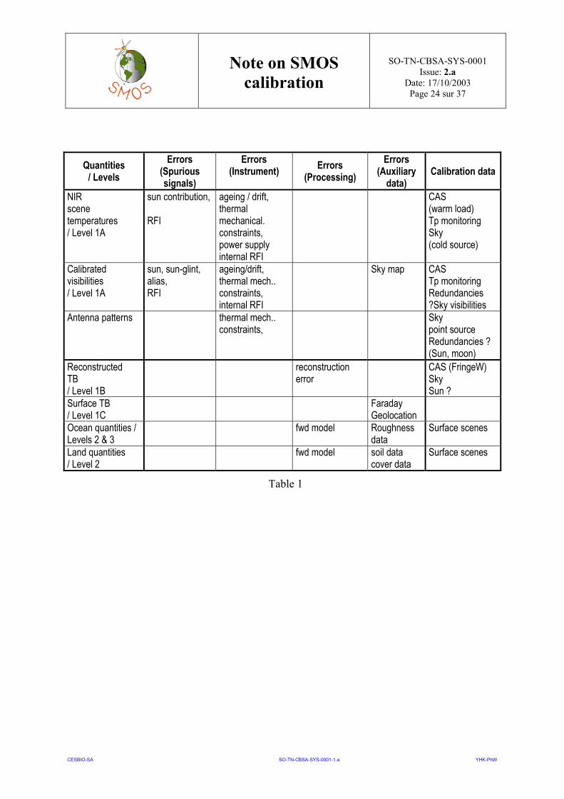
The next table (1) summarises the discussion in previous paragraphs: it sketches levels, errorsand their origins, possible expected calibration tools.

Random radiometric uncertainties are left out. They will have to be considered neverthelesswhen assessing the duration necessary to obtain meaningful Cal/Val SMOS measurements.



Date: 17/10/2003 sur 37


Quantities/ Levels

Errors(Spurioussignals)

Errors(Instrument) Errors

(Processing)Errors

(Auxiliarydata)

Calibration data

NIRscenetemperatures/ Level 1A

sun contribution,

RFI

ageing / drift,thermalmechanical.constraints,power supplyinternal RFI

CAS(warm load)Tp monitoringSky(cold source)

Calibratedvisibilities/ Level 1A

sun, sun-glint,alias,RFI

ageing/drift,thermal mech..constraints,internal RFI

Sky map CASTp monitoringRedundancies?Sky visibilities

Antenna patterns thermal mech..constraints,

Skypoint sourceRedundancies ?(Sun, moon)

ReconstructedTB/ Level 1B

reconstructionerror

CAS (FringeW)SkySun ?

Surface TB/ Level 1C

FaradayGeolocation

Ocean quantities /Levels 2 & 3

fwd model Roughnessdata

Surface scenes

Land quantities/ Level 2

fwd model soil datacover data

Surface scenes

Table 1



Date: 17/10/2003 sur 37


4. EXTERNAL IN-FLIGHT CALIBRATIONS FOR SMOS

4.1 LIMITATIONS OF EXTERNAL AND VICARIOUS CALIBRATION.

4.1.1 ERRORS ON THE SET OF SMOS DATA

Random errors have to be indeed very small in order to detect 0.03 K necessary to have 0.1psu in “average conditions”: over the ocean. The specification is at least the same as for themeasurement (not mentioning pointing and other sources of error). It is worth remembering thatequivalent random errors on TB are about 2 to 4 K for each pixel in a single reconstructedsnapshot (2 x 1.2 second), about 0.5 K when including multi-angular and dual polarisationvalues, slightly below 0.03 over a "GODAE" box, around 0.025 K over the whole field of view(also when including multi-angular and dual polarisation values).

The snapshot (one polarisation) random error over a scene temperature is about 0.06 K on eachinterferometric channel (about 0.09 K for the NIR); the same error is foreseen for normalisedvisibilities, noting that some correlation is present.

Systematic biases: they are not very likely to occur undetected. However, if calibration targetsare systematically acquired in specific conditions, biases may occur. This can be avoided withcalibration targets scattered at various locations along the orbit. Errors on calibration data sets

It is very likely that (at least) random errors will also be present in the calibration set, in whichcase the necessary number of data will be higher.

The accuracy of calibration data also has to be considered. We have the actual physicalvalues at the surface (with some uncertainty) and must reconstruct Tb through modelling withthe required accuracy. It is thus necessary to know perfectly well the direct mode as well asevery relevant surface parameter. It is also necessary to separate random and systematic errors(in the modelling as well). Finally, one must be aware that, especially when looking at extendedtargets, the required accuracy makes it necessary to account for contributions from theatmosphere, the ionosphere, and, in addition, to account for smearing effects on incidenceangles in SMOS data.

4.2 POST LAUNCH CALIBRATION SCHEMES

4.2.1 NIR COLD SOURCE CALIBRATION

4.2.1.1 THE FIELD OF VIEW PROBLEM

Although the NIR are classical radiometers, the main (specific) difficulty when consideringtheir external calibration is their wide field of view. Brightness temperatures must be integratedover a very large solid angle (representing about 2500 km on each side to reach grazingincidence), whereas when talking about calibration areas one mostly thinks in terms of dataavailable for calibration over a (comparatively) small area, the size of a few SMOS pixels.



Date: 17/10/2003 sur 37


4.2.1.2 SKY: ENGINEERING ISSUES

The sky is proposed to provide the external (cold) source. The integration time must allowbringing radiometric uncertainty down to levels compatible with the salinity measurements.This can probably be achieved using a few minutes.

It is anticipated that such measurements will require alternatively one orbit every 2 weeks.However the most critical performance is the NIR stability between calibrations, or moreexactly the adequacy of the correcting functions of the thermal monitoring data. To this end, itwill probably be necessary, during the commissioning phase, to increase the frequency of NIRcalibration operations above the nominal frequency quoted above. A prerequisite isnevertheless a complete and reliable modelling of the thermal behaviour and a good monitoringof internal temperatures during operations.

The sky is a good target in the sense that it is rather well known (Reich and Reich see also[14]), with the caveat that there are large sources to be accounted for, and that looking a the skyrequires manoeuvres, and may imply for the sensor-satellite system a different thermal regimewhich could lay outside the normal or modelled range. Moreover back-lobes may prove to be asignificant issue.

Concerning manoeuvres, the first idea was to slightly tilt the platform forward to view deep skythrough the top tip of the FOV. This was not deemed very useful, as it will be very difficult toavoid contribution from the Earth etc.

The other solution is thus to tilt completely the satellite so that it looks at zenith for calibrationpurposes.

It is now necessary to evaluate this possibility and to start identifying potential caveats so thatthe technical feasibility can be assessed together with the scientific outcome (i.e., improvementof calibration) wrt induced "costs" to the mission. Obviously we do not want to jeopardise themission.

The practicalities were described in [7] so we will not deal with them here as it is now in thehands of the project.

Similarly, we do not know yet how the sky observation will impact the thermal conditions ofthe payload.

4.2.1.3 TARGET KNOWLEDGE POWER REQUIREMENTS

Looking at the sky has no meaning unless we can be sure that we are looking at a source that isperfectly known. This raises 3 conditions:

� Avoid galactic sources; this is probably impossible a large fraction of the time. Then, thesky temperature is basically 2.7 K there are many sources contributing to 0.5 K above thecosmic background.

� check that the sun contribution is negligible



Date: 17/10/2003 sur 37


� Address successfully the issue of the rear lobe. This is probably difficult. Nothing much isknown about the rear lobe (since deep sky calibration was never considered) until fullanechoic chamber measurements are performed. Typically this might be very irregular. Therear lobe will collect emission from inhomogeneous sources (the visible part of the Earth isabout 5000 km wide, so the chances of homogeneous ocean everywhere are scarce). Ofcourse, there is also the variation with incidence angle. Assuming 25 dB below and anaverage 150 K up-welling TB, the resulting contribution would 0.5 K, probably impossibleto know within better than 10%. Preliminary antenna measurements suggest this ispessimistic as first measurements indicate about 40 dB.

Consequently the geometry will have to be carefully studied.

Provided the matter of the rear lobe is properly settled, the sky observation should provide acold source measurement with an accuracy better than most other calibration data, and wouldbe therefore very useful. More quantitatively, it appears that we should expect, when looking atthe deep sky scene, about 3.5 K from the front plus the rear lobe. There is no point in trying toachieve on the sky radiation a better performance than on the rear lobe contribution. Now, sincethe operational range for scene temperature is about 120 to 240 K, possibly the requiredaccuracy on the cold source is not drastic; this has to be evaluated form the NIR operationmodelling.

There is a possibility to obtain an independent information by assessing the standarddeviation of the measured brightness temperature. Then the necessary time would probably bemuch longer (TBD)

4.2.2 SEA SURFACE SCENES FOR NIR

The emphasis in this vicarious scheme is on the mean value of the retrieved salinity.Unfortunately we cannot expect to carry out the NIR calibration with such a scene. It wouldrequire an area of about 5000 x 5000 km homogeneous (temperature and salinity) with almostno wind. To achieve 0.03 K it is necessary to have an integration time of about 60 s (400 km)all without land in view.

It can be envisioned nevertheless to use ocean surface to be used with statistical vicariousmethod (see below 4.2.4).

4.2.3 SUN AS HOT SOURCE FOR NIR CALIBRATION ?

It has also been suggested to use the sun (if only to check possible drifts in hot load?) but itdoes not seem very either easy or relevant. The idea to use the sun during descending passwhen it is seen at the very edge of the FOV has also been suggested. This raises the issue of theantenna gain (how well known is it and impact on global error, and, even more an issue, the sunseen in this position might give too small a signal to be of significant value. Finally, theaccuracy with which the source is known is probably not sufficient.



Date: 17/10/2003 sur 37


4.2.4 STATISTICAL VICARIOUS CALIBRATION FOR NIR DRIFTS

So as to monitor potential instrumental drifts, we may rely on vicarious statistical approachesfor long term drifts

The idea at this level is to consider methods such as those developed for SMMR or SSM/I andfurther developed by C. Ruf (see [15]) the method is particularly applicable to SMOS as thenumber of acquisitions is quite significant.

Statistical approaches are believed to be particularly relevant for estimating trends anddetecting possible events. However the consideration of sea roughness effect still requiresanalysis. Statistically, a sufficient number of samples might be collected on time scales as smallas a few days. It seems that the accuracy of statistical vicarious calibration might reach about0.1 K.

4.2.5 DEEP SKY CALIBRATION OF VISIBILITIES OR TEMPERATURES

A synthetic map of visibilities when looking at the sky can be computed and compared toobserved level 1A data.

There are several reasons why considering visibilities rather than brightness temperatures. Theradiometric uncertainty on SMOS data is then fairly low.

Mainly, we must keep in mind that while the ultimate purpose of calibrating the interferometeris to correct for possible inhomogeneities of the instrument response curve throughout theFOV, actual misalignments of the instrument parameters will be located in channels andbaselines, and therefore much less difficult to locate when calibration data are provided interms of visibilities.

Visibilities radiated by the sky scene have to be computed from sky temperature maps providedby radio-astronomy surveys; this will introduce uncertainties over calibration data. Howeverthe radiometric errors on SMOS snapshot TB field are so large that the option to work in thevisibility domain seems the only practical one. Moreover, if one were to go into thereconstructing process, the alias free zone would be smaller than when looking at the Earth,since there would be no way to extend it to cases where ambiguous zones origin from the sky,as the sky is the target itself.

As mentioned in section 3, if the a priori knowledge of the sky map needs confirmation, thenthis operation allows to some extent control of one part of the sky map and of its stability intime.

Alternatively, the aim will be to check instrument parameters, check the consistency ofredundant visibility samples. For N interferometric channels, sky calibration provides N2

accurate data per polarisation (including PMR outputs); the optimum way to use this data setcalls for a specific study.

As indicated above, it is necessary to check that the thermal regime of the interferometer whenlooking at the deep sky stays within normal operating conditions. (i.e., not outside thecapabilities of the thermal control)



Date: 17/10/2003 sur 37


This calibration step, although aimed at the interferometer, implies the use of the NIRradiometer. The same operation, however, allows (see below) to provide a cold source for theNIR. Assuming the errors on sky L band surveys are random and can be averaged over thesolid angle pattern, the temperature of the sky scene would be known to better than 0.01 K.

4.2.6 VICARIOUS CALIBRATION OF THE INTERFEROMETER

4.2.6.1 OPEN SEA SCENES

If a sufficiently homogeneous sea area could be found (including weak and homogeneous searoughness, total absence of coasts and islands, no sun contamination whatsoever), andsatisfactorily covered by surface measurements, a vicarious interferometer calibration could beconsidered on level 1C. The necessary area is at least 5000 km wide in every direction. Such anapproach is not realistic.

The radiometric uncertainty will be large, therefore this calibration will use as much alongtrack averaging as possible and should be compounded over several orbits.

However, a nicely placed island of known characteristics and adequate size might be useful as apoint source.

This calibration step, although aimed at the interferometer, implies the use of both the NIRradiometer and a forward ocean surface model. Its specific use here consists of detectinginhomogeneities in the retrieved salinity maps whereas the ground truth is homogeneous. Thismight give hints about some instrumental errors.

The possibility of detecting residual effects (after on board calibration) from surface calibrationdata needs to be assessed (This is a case where the SEPS could be put to good use to simulatedifferent calibration frequencies)

4.2.6.2 OTHER POSSIBLE SURFACE TARGETS

The only realistic use of such limited targets is to perform a complete calibration (on either SMor OS) covering the NIR, the interferometer and eventually the direct model. One should neverthe less bear in mind that the radiometric accuracy for 1 pixel (30 angles and 2 polarisation isroughly 0.5 K. The scene has to be known and possibly homogeneous of course and the directmodel accurate. If the target can be extended the figure can be improved (SQRT of number ofindependent samples). So as to satisfy the different requirements the number of options is verylimited [9] The first options which can be considered are:

� The area on Antarctica around Dome C

� Well monitored "homogeneous" area over land (large test site with extensive groundmeasurements)



Date: 17/10/2003 sur 37


4.2.7 POINT SOURCES

4.2.7.1 PURPOSES

There are several purposes in the use of point sources:

One is to be able to verify / characterise the antenna diagrams, for this the best potentialsource is the sun if we know its evolution quite well. Ideally the sun should be scannedthrough the bore-sight

A second is for the DLR reconstruction method. The point source (sun) is scannedthroughout the FOV so as to be seen in every pixel2. From current information this does notseem really feasible.

A third is for calibrating the radiometer. Such point sources are to be known and to befound in a cold background. In this context, we can disregard the moon. Sun is certainly anoption but it requires important manoeuvres (and imply severe constraints on theinstrument). Using the sun when at the extreme of the FOV is not practical for this purpose.

To assess the interferometer the moon may be useful as a relatively weak source (equivalentto 10 K over a known background (3-6 K) but this has to be studied further. The Sun in thiscase is probably not fully adequate (relatively strong and messy).

4.2.7.2 USING THE MOON AND / OR THE SUN

So as to have an external / vicarious calibration target for SMOS, the possibility to use theMoon and the Sun as point sources was considered. Even though this option is still under studyit is necessary to estimate the requirements for the mission specifications. It should be notedthat there are other potential sources (Cygnus for instance, which is at least 15 times higherthan the Moon) but here again the feasibility is to be studied.

The Moon and the Sun offer the possibility to view a "hot" point source with a coldbackground. This being said things are not so simple as:

The background is not that uniform and can vary significantly wrt to the target position.

The Sun's emission does vary significantly with time. If we do not have easy access to datafrom monitoring centres (i.e., accurate monitoring 1% expected?), such target can only beused as a hot source vs cold background (i.e. interferometer calibration). Actually the Sun ismonitored at L band but we are going towards an “active period” for the Sun.

The Moon also varies with time (if only Moon phases and reflected solar contribution about1% on average?), and its brightness temperature is not fully known. Moreover it is not veryhigh ( 250 K) and, as the Moon (and Sun) intercepts a small percentage of a basic "pixel"(about 6 %) the contrast will be even smaller (about 15 K)

2 A single diagonal pass done from time to time could eventually be used but this option has to be studied furtherboth in terms of feasibility and of interest



Date: 17/10/2003 sur 37


4.2.7.3 SYNTHESIS

It seems that the Moon is not a good candidate but the Sun is maybe the only possibility to beable to measure in flight the co-polar antenna diagrams. For this we need to know the sourcestability, follow the sun and have stable NIR. This point is thus still to be studied.

Such external calibration is possible but with an outcome that is not 100% ascertained. Wesuggest considering this option further, but, in the mean time, no hard constraints should be puton the mission, as the current characteristics seem sufficient.

One should keep in mind during this calibration exercise that we will have eventually to copewith the following constraints:

1. The SMOS mission is aimed at providing data globally and frequently: the calibrationshould take only a small portion of the time.

2. When moving the platform (towards the sun or the sky or whatever), we may be in aconfiguration where downloading is not possible which may jeopardise even the dataacquired itself

3. Manoeuvres consume fuel and hence reduce lifetime if too frequent.

4. Manoeuvres change completely the thermal constraints and hence may distort measurementor damage the PLM.

5. And finally, as already stated, back-lobes may be an issue.

As per the sources themselves, the conclusions may be that:

The Moon is not useful (TBC) for calibrating the NIR elements and interferometer (smallcontrast over the large main lobe; side and back lobes contributions to be taken intoaccount)

The Sun might be useful as a point source target. But in this case:

Only use the Sun when "calm" or if monitoring data is available (which should notbe a problem TBC)

Investigate the feasibility of using the sun “seen on the side”

This would require:

Fine choice of occurrences when optimal viewing conditions are met

Finally checking for other radio-sources might be useful but, when observed, the targetsshould be in a "calm" area in terms of galactic noise (i.e. avoid galactic plane) and in knownareas.



Date: 17/10/2003 sur 37


4.3 SEA SURFACE NETWORK (VICARIOUS) CALIBRATION/ VALIDATION

This method which could be considered as a validation as is uses geophysical data andretrievals, is actually using multiple acquisitions of both satellite and ocean measurements tocalibrate in a sort of assimilation mode the system. The idea is to gather data over a large rangeof SST SSS and WS and assimilate them to compare with retrievals. More details are given inthe validation part.

It must be clear that ultimately the consistency between SMOS salinities and data provided by asurface network will be required. Due to the accuracies of in situ salinity and temperaturemeasurement, and provided the range of the sea roughness can be restricted, bearing in mindthat then the surface is homogenous on large scales, it is felt that adequate samples of thesurface network data will turn out to be the main calibration driver.

While this approach is unavoidable and should be the most conclusive, it may turn out to bevery complicated. Through direct comparison between surface data and level 2 retrievals, onehopes at the same time to check the NIR calibration, to account for possible inhomogeneities ofthe interferometer response, and to tune (with some degree of empirical fitting) the retrievalalgorithm, This calls for a carefully designed process.

4.4 SMOS AQUARIUS / HYDROS INTERCALIBRATION

SMOS is a stand-alone project but as for any other such project many gains will be available iftwo similar missions fly together (see ERS tandems Vegetation and SPOT tandem scenarii etc).There will be also a unique opportunity for both calibration and possibly validation to useeither Aquarius or HYDROS should they fly at the same time as SMOS. Already, withAquarius, plans are being made to share common approaches (see 5.3). The simplest way tointer-calibrate is to compare separately to the same surface data each time the acquisitions aresynchronous. However it may be worth attempting to avoid the vicarious step included in thisapproach. Both systems, having real antennas will provide measurements with quite differenterror sources when compared to SMOS, and a higher sensitivity. This might proved to be theultimate external calibration source

This part will thus have to be expanded once more is known on the two other missions.

4.5 SUMMARY TABLE

The following (draft) table proposes external calibrations together with purposes, difficultiesand aims. Filling adequately this kind of table might be proposed as a first test for theconsistency of the calibration document.



Date: 17/10/2003 sur 37


Target purposes Implementationproblems

SMOS dataproblems

Targetproblems

Hoped forperformance

Deep skyscene

Cold source forNIR

rotation everymonthstability

Knowledge oftargetback lobe

down to 0.15 K?

Sea scene(vicarious)

NIR None Find it…fwd model andknowledge

None: internalwarm load

Check NIRcorrecting laws

Frequent duringcommissioning

none none down to 0.03 K

Deep sky onvisibilities

Check sky map

MIRAS errors

rotation everymonth

stabilitythroughoutrotation;

stabilityback lobeRandom errorsKnowledge oftarget

Deep sky onTB

Check sky map

MIRAS errors

rotation everymonth

Random errorsFOV

ditto Difficult tointerpret

Sun on scenetemperature

antennapatterns

Rotation and tilt? Power stability less than 1% ofaxis gain

Sun onvisibilities

MIRAS transferfunction

Rotation and tilt? backgroundscene

TBD

MoonOther sources Antenna

patternsrotation stability Back lobes

Antarctic (vic) Every error None Random error fwd modelSea area (vic) overall None Random error fwd modelLand area (vic) overall None Random error fwd model

RFIOcean network(vicarious)

overall Data access Random error select sample Down to 0.03 Kfor 300 datapoints

statistical TB(mean, median,tail slope)(stat vicarious)

overallcalibrationdrift

possible frequencyup to 1 per a fewdays

remove flaggeddata

everygeophysicalerrorSea state (tbc)

down to 0.1 K

SMOS vsAQUARIUS

overall? synchronousobservations

TBD

Table 2



Date: 17/10/2003 sur 37


5. VALIDATION: FIRST PRACTICAL SUGGESTIONS

5.1 MEASUREMENTS TO BE USED IN VALIDATION.

Over the ocean, the main validation parameter is sea surface salinity. Inasmuch as wind speedis a secondary retrieved parameter, it may be considered for validation.

Over land, the main validation parameter is soil moisture. Inasmuch as vegetation opticalthickness is a secondary retrieved parameter, it may be considered for validation. Howeverthere is no reliable ground truth measurement for both variables.

Both over sea and land, it is expected that several hundred measurements are available everyday

The SMOS measurement uncertainty for a single pixel measurement, due mainly to radiometricsensitivity, is of the order of 1 PSU for salinity and 4% for soil moisture.

5.2 SCALE ISSUES

A major limitation is due to the fact that SMOS measurements concern an area of size about 40km, while ground truth essentially consists of point measurements. For validation it will benecessary to either monitor exhaustively a very large area (at least 100 km) of fairlyhomogeneous surface

Over the ocean, this is not of too much consequence, as the scale of variation of sea surfaceconditions is larger than that at least for salinity and SST. However care should be exercisedconcerning wind conditions

Over land, It is necessary to identify areas as homogeneous as possible. Privileged validationsites should include a network of ground sensors, so as to characterise the actual sub-pixelvariability of soil moisture. Several such sites do exist currently but are adequate at differentlevels (long term or type of measurements routinely performed) and will be evaluated in depthduring the Cal/Val preparatory programme.

5.3 SEA SURFACE NETWORK CALIBRATION / VALIDATION

Ground data measurements over sea are the only ones to offer an adequate accuracy to performabsolute calibration/validation of the SMOS payload.

Assuming that several hundred surface measurements spread over the whole oceans areavailable every day, the main Cal/Val scheme consist of removing pixels flagged for any event(heavy rain, sun image) and carrying out a multivariate statistical analysis in order to detectpossible trends depending on sea roughness, wind direction, latitude, season.

It is therefore necessary that surface data cover wide ranges for all these variables.

Surface data available should be used partly (initially) for tuning the sea surface algorithm,partly for validation.

As a result, all land ground data and about 2/3rd of sea surface data should be available forvalidation.



Date: 17/10/2003 sur 37


5.4 DYNAMIC RANGE AND VERSATILITY OVER LAND

Accounting for the complexity of forward modelling and the measurement uncertainty, singlepoint measurements are inadequate. The calibration strategy should provide large time series,allowing to sample a large dynamic range of both soil moisture and vegetation cover overland, and provide large numbers in order to allow statistical analysis.

Over land, possible biases will come from erroneous auxiliary parameters (soil structure, forestthickness)

5.5 LAND PIXEL OTHER THAN VEGETATED SOIL

There is a possibility to use other surface types such as very large areas at high latitudes, rainforests, large ice sheets (Antarctica), but it is clear that each one of them poses various types ofdifferent problems, some being very delicate to cope with. Specific studies will most probablybe necessary before assessing exactly the validity of such targets especially as we will not bedealing necessary with SM or opacity.

A special mention should also be made of other methods that even though they might notvalidate per se the products, might help in giving some confidence. We are thinking of modeloutputs, retrievals from other satellites, analysis of time series etc…



Date: 17/10/2003 sur 37


6. CONCLUSIONSThis document intends to be a first step towards the definition of a calibration procedure forSMOS. It is intended thus to be a working document open for discussions. It seems that forachieving a good calibration we will have to work on several levels, which are unfortunatelyclosely interrelated with all the complexity it will entail.

The first point is the instrument calibration itself with both the hardware (i.e., antenna+receivers) and interferometry. This will not be sufficient and vicarious calibration will berequired as well, leading to specific issues as explained above (targets, temporal variations,modelling). These issues can only be addressed through further studies and use of the end toend simulator.

The second point is related to the protocol for external / vicarious calibration. The issues arelinked to the choice of suitable targets (i.e., size, stability and knowledge) and correspondingtime scales. If long-term stability could probably be addressed with use of time/space averages(with the caveat of climatic trends) short-term stability will have to be derived (requiring beingable to simulate the orbit cycling).

The third point is the distinction between absolute and relative calibration. The first onerequires a large target to be viewed (and known) and very good NIR. Relative calibration willrequire a good knowledge and modelling of the instrument (errors in receivers will translateinto errors in Tbs) and of the reconstruction. It will be necessary to use long-term calibrationhere as well (random errors precludes the use of "single shot" acquisitions).

It must be noted that this document does not cover yet completely effects linked to abnormalevent such as RFI or sun glint and sun aliases etc in the field of view.

Similarly the special issue of "thresholding" and flagging special events (heavy rain, TEC bursteven solar flares, or large rain water ponds, etc.. it yet to be addressed.

So to summarise, the main conclusions are that the main calibration points should be:

� Before flight:

A complete and very detailed characterisation of the SMOS System with an accuracycompatible with the radiometric requirements when computed /estimated for orbitalenvironment including:

� Antenna patterns

� Thermal behaviour (hence accurate instrument model) and means to monitorit in flight.

� During flight



Date: 17/10/2003 sur 37


� The on-board calibration should be sufficient to monitor and adjust the aboveparameters.

� Make full use of the on-board calibration.

� Do not put any constraints related with the use of the moon as a target which could onlybe useful for visibilities

� The assimilation of buoys data (and possibly AQUARIUS/HYDROS acquisitions) areprobably the safest methods

� Some ground targets might be of use

� Viewing deep sky will certainly be useful but not self sufficient

� A reliable point source will be necessary. The sun is probably the best candidate but itraises many an issue. It certainly needs further studies.

This note is yet to be improved. Table 2 should be probably used to ascertain the priorities.Finally this document is incomplete. It lacks much information on the payload itself and doesnot give many quantitative requirements. It may also give the impression that several redundantapproaches are presented. Considering the complexity of the task to calibrate and validateSMOS, we believe that, any option, which has no large impact on the system, should bepursued.

so-tn-cbsa-sys-0001 note on smos yhk & · pdf filephilippe waldteufel sa approved by: cnes...

Documents