Social Learning and Solar Photovoltaic Adoption:Evidence from a Field Experiment∗

Kenneth Gillingham† Bryan Bollinger‡ Hilary Staver§

Preliminary and Incomplete–Do Not CiteSeptember 8, 2015

Abstract

An extensive literature points to the importance of social interactions in influencingeconomic outcomes. We examine a set of natural field experiments on a rapidly ex-panding behavioral intervention designed to actively leverage social learning and peerinteractions to promote solar photovoltaic technology in Connecticut. The “Solarize”program involves a municipality-chosen solar installaller, group pricing, and an infor-mational campaign driven by volunteer ambassadors. We show that the program isremarkably effective: a treatment effect increasing installations by 27 per municipal-ity on average, increasing installations by over 100 percent. The program also lowersinstallation prices, an effect that spills over to adjacent block groups. When munici-palities are chosen randomly, the treatment effect is roughly half. However, this stillexceeds the treatment effect from a program run by a single installer without compet-itive bidding. Calculations reveal that the Solarize program is cost-effective and socialwelfare-improving. Survey results illuminate the mechanisms underlying our findings.

Keywords: non-price interventions; social learning; renewable energy; solar photo-voltaic panels; technology adoption; natural field experimentJEL classification codes: D03, L22, Q42, Q48

∗The authors thank Josh Graff-Zivin for useful comments. We also thank Brian Keane, Toni Bouchard,Lyn Rosoff, Kate Donnelly, Bernie Pelletier, Bob Wall, Robert Schmitt, Stuart DeCew, Jen Oldham Rogan,and the Yale student team working on the SEEDS project for support on this project. The authors wouldalso like to acknowledge funding from the U.S. Department of Energy.†Yale University and NBER, 195 Prospect Street, New Haven, CT 06511, phone: 203-436-5465, e-mail:

kenneth.gillingham@yale.edu.‡Duke University, Fuqua School of Business, 100 Fuqua Drive, Durham, NC 27708, phone: 919-660-7766,

e-mail: bryan.bollinger@duke.edu.§Energy and Environmental Economics, Inc., 101 Montgomery Street, Suite 1600, San Francisco, CA

94104, phone: 415-391-5100, e-mail: hilary.staver@ethree.com.

1 Introduction

mention percent of ground-mounted systems in discussion of Geostellar data.

Economists have become increasingly interested in behavioral interventions or “nudges”

that encourage actions that are privately or socially beneficial. Such interventions often

involve information provision that includes social comparisons or pro-social appeals. This

is especially true for the voluntary provision of public goods, such as environmental public

goods (Allcott and Rogers, 2015; Ferraro and Price, 2013). At the same time, there is

mounting evidence that social interactions themselves, through social learning and peer

effects, influence the adoption of environmentally-friendly technologies (e.g., Bollinger and

Gillingham, 2012).

This study uses a natural field experiment (Harrison and List, 2004) to examine a rapidly

expanding behavioral intervention in the United States designed to leverage the power of so-

cial interactions to promote a fast-growing renewable energy technology: solar photovoltaic

(PV) installations. The “Solarize” program is a community-level behavioral intervention

with several key pillars. Each treated municipality chooses a single solar PV installer based

on the group pricing deal offered in bids from installers. The intervention begins with a

kick-off event and involves roughly 20 weeks of community outreach. Notably, the pri-

mary outreach is performed by volunteer resident “solar ambassadors” who encourage their

neighbors and other community members to adopt solar PV. This social interaction-based

approach parallels previous efforts to use ambassadors as “injection points” into the social

network to promote adoption of agricultural technology (BenYishay and Mobarak, 2014;

Vasilaky and Leonard, 2011) and behavior conducive to improving public health (Kremer,

Miguel, Mullainathan, Null and Zwane, 2011; Ashraf, Bandiera and Jack, 2015) in developing

countries.

In this paper, we ask several questions that shed light on consumer and market behavior

under the influence of a large-scale behavioral intervention. Is such a program effective at

increasing adoption of solar PV and lowering installation prices? Do these effects persist

1

after the intervention? Are there spillovers or positive treatment externalities to nearby

communities (Miguel and Kremer, 2004)? How cost-effective is the program for meeting

policy goals, and is it welfare-improving? These research questions have important policy

relevance, for Solarize or similar interventions are currently being implemented in many

states, and many others have expressed interest in the program to help meet climate and

energy goals.1 In fact, there is even a well-publicized program guidebook for policymakers

interested in implementing a Solarize program (Hausman and Condee, 2014).

We establish the effectiveness of the Solarize program using two randomized controlled

trials (RCT) and a set of trials with rolling control groups, as in Sianesi (2004) and Harding

and Hsiaw (2014). We first examine municipalities that apply to join the program, for these

are the marginal municipalities when such a program is expanded elsewhere. For these

municipalities, we find that the treatment leads to 27 additional installations over the course

of a campaign on average, an increase of over 100 percent from the counterfactual. There

is also considerable variation across campaigns; for example, we estimate a treatment effect

of 53 additional installations from the first round of the campaign, an increase of over 370

percent from the counterfactual. Post-treatment, we find no evidence of either a harvesting

effect (e.g., as occurred with the well-known Cash for Clunkers program (Mian and Sufi,

2012)) or further induced installations, which might be possible due to continued social

learning or peer effects.

We find that the program lowers the equilibrium price during the Solarize campaigns

by roughly $0.64 per watt (W) out of a mean price of roughly $4.61/W in the control

municipalities.2 Moreover, our results suggest the presence of treatment externalities that

lower the equilibrium price in neighboring Census block groups by $0.15/W, but only increase

installations by 1 to 2 installations per municipality. In fact, our treatment effect results do

not change when including the price as a covariate, indicating that the discount pricing in

1Implementing states include Oregon, Washington, California, Colorado, South Carolina, North Carolina,Ohio, Pennsylvania, New York, Rhode Island, Massachusetts, and Vermont.

2All dollars in this paper are 2014$.

2

the treatment is only a small part of the explanation for the effect.

Our second RCT involves randomly selected municipalities across CT, rather than mu-

nicipalities that applied to participate in the program. Nearly all of the municipalities we

approached agreed to join the program. The estimated treatment effect is roughly half of the

treatment effect estimated for the municipalities that opted-in, both in terms of installations

and prices. This finding provides guidance for policymakers who would consider scaling up

such a program beyond the municipalities that self-select by applying.

We examine the mechanisms underlying the effectiveness of the treatment in two ways.

First, we examine an installer-led program, called “CT Solar Challenge,” (CTSC) that in-

cluded all of the central tenants of the Solarize program except the involvement of state

government and the competitive bidding process. This allows us to test the hypothesis that

competitive bidding is necessary for the effectiveness of the campaign. We estimate a small

treatment effect of CTSC leading to more installations, but no effect on prices in the first

six months, and only an effect afterwards when it was clear that CTSC was not bringing in

many new leads. This result provides insight into the age-old question in economics of how

the institutional structure of markets influences pricing and other market outcomes. Second,

we survey participants in the Solarize program, and find that measures related to social

influence, such as “speaking with friends and neighbors” or “interactions with the social

ambassador,” are rated as extremely important factors in the decision to install solar. This,

combined with the finding that including price does not change the estimated treatment

effect on installations, provides suggestive evidence that the Solarize behavioral intervention

works primarily by leveraging social interactions.

Our results have clear policy implications. Behavioral interventions based on informa-

tion, word-of-mouth, persuasion, and other non-price approaches have become increasingly

popular for encouraging prosocial activities, and community-based interventions are perhaps

the latest vanguard of this movement among practitioners (McKenzie-Mohr, 2013). With

billions of dollars spent each year by electric and natural gas utilities on energy conservation

3

(Gillingham and Palmer, 2014) and billions more by federal and state governments on pro-

moting adoption of solar PV (Bollinger and Gillingham, 2014), evaluating the effectiveness,

persistence, and cost-effectiveness of these rapidly expanding community-based programs is

important for policy development.

In our setting, we find that each additional installation due to the program costs roughly

$900 in funding, which can be compared to typical estimates of installers’ customer acqui-

sition costs of $0.48/W (Friedman, Ardani, Feldman, Citron, Margolis and Zuboy, 2013),

amounting to $1,500 to $3,000 for an installation, or an average consumer savings of $4,627

from the program. The cost-effectiveness per ton of CO2 reduced depends on assumptions

about the future carbon intensity on the New England electric grid. Assuming the 2012

CT carbon intensity from EIA (2014) remains constant into the future, this implies a cost-

effectiveness estimate of $32 per ton of CO2 avoided based only on the direct costs of the

intervention. If the CT carbon intensity decreases rapidly with increased natural gas use

or if other subsidies are included, this estimate may be significantly higher. From an eco-

nomic efficiency standpoint, we deem it quite likely that by acting as a “nudge” to encourage

prosocial behavior, the Solarize programs increase social welfare.

This paper is organized as follows. Section 2 describes the empirical setting, our hy-

potheses, and our randomization. Section 3 presents our dataset and descriptive summary

statistics, while section 4 describes our estimation strategy. Section 5 presents the results

and section 6 the cost-effectiveness calculations. Section 7 concludes with a discussion of

implications for policy.

2 Research Design

This paper leverages a unique experimental setting to test several hypotheses about the

rapidly-expanding Solarize behavioral intervention. Before moving to these hypotheses, it is

useful to first provide some background on solar PV in CT and the Solarize program itself.

4

2.1 Empirical Setting

CT has a small, but fast-growing market for solar PV, which has expanded from only three

installations in 2004 to nearly 5,000 installations in 2014. Despite this, the cumulative

number of installations remains a very small fraction of the potential; nowhere in CT is it

more than 5 percent of the potential market and in most municipalities it is less than 1

percent.3 The pre-incentive price of a solar PV system has also dropped substantially in the

past decade, from an average of $8.39/W in 2005 to an average of $4.44/W in 2014 (Graziano

and Gillingham, 2015).

Despite being in the Northeastern United States, the economics of solar PV in CT are

surprisingly good. While CT does not have as much sun as other regions, it has some of the

highest electricity prices in the United States. Moreover, solar PV systems in CT are eligible

for state rebates, federal tax credits, and net metering.4 For a typical 4.23 kW system in

2014, we calculate that a system purchased with cash in southern CT would cost just under

$10,000 after accounting for state and federal subsidies and would have a internal rate of

return of roughly 7 percent for a system that lasts the expected lifetime of 25 years (See

Appendix 1 for more details on this calculation and some sensitivity analysis).

Thus, solar PV systems display the properties of a classic new technology in the early

stages of the process of diffusion (e.g., Griliches, 1957). From a private consumer perspec-

tive, solar PV systems are very often an ex ante profitable investment. This is important in

the context of this study, for it indicates that Solarize campaigns are “nudging” consumers

towards generally profitable investments. There of course will be heterogeneity in the suit-

ability of dwellings for solar PV and we are careful to focus on the potential market based

on satellite imaging from Geostellar (2013). We will discuss the social welfare implications

in Section 6.

3Estimates based on authors’ calculations from solar installation data and potential market data basedon satellite imaging from Geostellar (2013).

4Net metering allows excess solar PV production to be sold back to the electric grid at retail rates, witha calculation of the net electricity use occurring at the end of each month. Any excess credits remaining onMarch 31 of each year receive a lower rate.

5

2.2 The Solarize Program

The Solarize program in CT is a behavioral intervention with several components, each

motivated by theory. At its core, the program focuses on facilitating social learning and

peer influence. Peer influence has been demonstrated to speed the adoption of many new

technologies and behaviors, including agricultural technologies (Foster and Rosenzweig, 1995;

Conley and Udry, 2010), criminal behavior (Glaeser, Sacerdote and Scheinkman, 1996; Bayer,

Pintoff and Pozen, 2009), health plan choice (Sorensen, 2006), retirement plan choice (Du-

flo and Saez, 2003), high student performance (Sacerdote, 2001; Duflo, Dupas and Kremer,

2011), foreclosure choices (Towe and Lawley, 2013), contraceptive adoption (Munshi and

Myaux, 2006), and even welfare participation (Bertrand, Luttmer and Mullainathan, 2000).

Bollinger and Gillingham (2012) and Graziano and Gillingham (2015) find evidence of neigh-

bor or peer influence on the adoption of solar PV technology in California (CA) and CT

respectively.

The first critical component to the Solarize program is the use of volunteer promoters or

ambassadors to provide information to their community about solar PV. There is growing

evidence on the effectiveness of promoters or ambassadors in driving social learning and

influencing behavior (BenYishay and Mobarak, 2014; Vasilaky and Leonard, 2011; Kremer

et al., 2011; Ashraf et al., 2015). Why might volunteer community members be effective

in Solarize? There is a robust economic literature on the importance of trust and trust-

worthiness in influencing economic outcomes by reducing transactions costs and building

social capital (Arrow, 1972; Knack and Keefer, 1997; Fehr and List, 2004; Karlan, 2005).

Furthermore, there is evidence that trust is enhanced by social connectedness (e.g., Glaeser,

Laibson, Scheinkman and Soutter, 2000; List and Price, 2009). Since the Solarize campaigns

are based at the community-level, social connectedness is more likely to be high. Moreover,

since the ambassadors are volunteers, they may be more likely to be seen as more trustworthy

by other community members.

The second major component to the Solarize program is the focus on community-based

6

recruitment. In Solarize, this consists of mailings signed by the ambassadors, open houses to

provide information about panels, tabling at events, banners over key roads, op-eds in the

local newspaper, and even individual phone calls to neighbors who have expressed interest

by the ambassadors. Jacobsen, Kotchen and Clendenning (2013) shows that a community-

based recruitment campaign can increase the uptake of green energy using some (but not

all) of these approaches. Kessler (2014) shows that public announcements of support can

increase public good provision, which perhaps may apply to the ambassadors in this setting.

The third major component is the group pricing discount offered to the entire community

based on the number of contracts signed. This provides an incentive for early adopters to

convince others to adopt and to let everyone know how many people in the community

have adopted. In this sense, it is intended to build social pressure and create a social norm

around solar PV in the community. There is strong evidence from consumer decisions about

charitable contributions that indicates consumers are more willing to contribute when others

contribute (Frey and Meier, 2004; Karlan and List, 2007; DellaVigna, List and Malmendier,

2012). Moreover, there is building evidence demonstrating the effectiveness of social norm-

based informational interventions to encourage electricity or water conservation (Allcott,

2011; Allcott and Rogers, 2015; Ferraro, Miranda and Price, 2011; Ferraro and Price, 2013;

LaRiviere, Price, Holladay and Novgorodsky, 2014). The choice to install solar PV is a

much higher-stakes decision than to contribute to a charity or conserve a bit on electricity

or water, so it is not obvious that effects seen in lower-stakes decisions apply. However,

Coffman, Featherstone and Kessler (2014) show that provision of social information can have

an important impact even on high-stakes decisions such as undertaking teacher training and

accepting a teaching job.

The fourth major component is the limited time frame for the campaign. Along with

group pricing, this fosters goal-setting since there is a limited time available to reach the lower

price tiers. Non-binding goal setting has been shown to influence energy conservation (Hard-

ing and Hsiaw, 2014), consistent with significant empirical evidence of reference-dependent

7

preferences (Camerer, Babcock, Loewenstein and Thaler, 1997; Crawford and Meng, 2011;

Pope and Schweitzer, 2011). Of course, the group pricing and limited time frame may also

provide a motivational reward effect (Duflo and Saez, 2003) for the price discount would be

expected to be unavailable after the campaign. Recent reviews (Gneezy, Meier and Rey-Biel,

2011; Bowles and Polania-Reyes, 2012) suggest that monetary incentives can be substitutes

for prosocial behavior, but by providing a prosocial reward that helps all, it is quite possible

that the two are complements in this situation.

Thus, the program is designed as a package that draws upon previous evidence on the

effectiveness of social norm-based information provision, the use of ambassadors to provide

information, social pressure, prosocial appeals, goal setting, and motivational reward effects

for encouraging prosocial behavior.

Facilitating the Solarize program in CT is a joint effort between the a state agency, the

Connecticut Green Bank (CGB), and a non-profit marketing firm, Smartpower.5 A standard

timeline for the program is as follows:

1. CGB and Smartpower inform municipalities about the program and encourage town

leaders to submit an application to take part in the program.

2. CGB and Smartpower select municipalities from those that apply by the deadline.

3. Municipalities issue a request for bids from solar PV installer for each municipality.

4. Municipalities choose a single installer, with guidance from CGB and Smartpower.

5. CGB and Smartpower recruit volunteer “solar ambassadors.”

6. A kickoff event begins a 20-week campaign featuring workshops, open-houses, local

events, etc. coordinated by Smartpower, CGB, the installer, and ambassadors.

7. Consumers that request them receive site visits and if the site is viable, the consumer

may chose to install solar PV.

8. After the campaign is over, the installations occur.

5The programs were funded by the CGB, The John Merck Fund, The Putnam Foundation, and a grantfrom the U.S. Department of Energy.

8

In this study, the Solarize campaigns are staggered into four rounds for logistical rea-

sons. Each round has several municipalities included. In the first round, nine municipalities

submitted applications and only four were selected, allowing for a randomization at the ap-

plication level (Step 2 in the timeline above). In the subsequent rounds, there was never

more than one or two additional applicants, so randomization was not possible.

However, we ran a second randomized experiment where the municipalities were selected

from a list of all non-Solarize municipalities in CT. Smartpower then approached these

randomly selected municipalities and were able to convince all but one to apply to take part

in the program. Everything else about the program was identical to the other chosen towns.

Finally, Aegis Solar created and funded the non-profit CTSC to contact municipalities

and encourage them to participate in a very similar campaign. Three municipalities agreed

to participate in the initial set of CTSC campaigns that began during a similar time frame

as the second round of Solarize. These CTSC campaigns are modeled after Solarize, as Aegis

Solar took part in the first round of Solarize and thus was very familiar with the program.

One very important difference is that there was no competitive bidding process. A second

difference is that CGB and Smartpower were not involved.

Table 12 lists the timeline of the treatment campaigns in this study. Figure 1 provides a

map of the 169 municipalities in CT, illustrating the 34 treated municipalities in this study.6

2.3 Hypotheses

Based on the previous literature and the design of the study, we had five hypotheses about

the Solarize program:

1. The intervention will substantially increase installations due to the combination of

program features designed around theories in the literature.

2. The intervention will lead to lower prices due to the group pricing discount, which is

6Some contiguous municipalities are run as joint campaigns, such as Mansfield and Windham in order toreduce costs. However, both municipalities still receive the full treatment.

9

made possible by economies of scale and lower consumer acquisition costs.

3. The intervention will lead to treatment externalities to adjacent municipalities through

word-of-mouth, which would lower prices and increase installations.

4. The intervention will be more effective at increasing installations in municipalities that

select into the program, but will also increase installations and lower prices in randomly

selected municipalities that agree to join the program.

5. The CTSC intervention will be less effective and not lead to lower prices, due to the

lack of competition and perhaps due to an institutional structure less conducive to

trust (Bohnet and Huck, 2004).

3 Data

3.1 Data Sources

The primary data source for this study is the database of all solar PV installations that

received a rebate from the CGB. When a contract is signed to perform an installation in CT,

the installer submits all of the details about the installation to CGB in order for the rebate to

be processed. As the rebate has been substantial over the the past decade, we are confident

that nearly all, if not all, solar PV installations in CT are included in the database.7 For each

installation the dataset contains the address of the installation, the date the contract was

approved by CGB, the date the installation was completed, the size of the installation, the

pre-incentive price, the incentive paid, whether the installation is third party-owned (e.g.,

solar lease or power-purchase agreement), and additional system characteristics.

The secondary data source for this study is the U.S. Census Bureau’s 2009-2013 American

Community Survey, which includes demographic data at the municipality level. Further, we

include voter registration data at the municipality level from the CT Secretary of State

7The only exception would be in three small municipal utility regions: Wallingford, Norwich, and Bozrah.We expect that there are few installations in these areas.

10

(SOTS). These data include the number of active and inactive registered voters in each

political party, as well as total voter registration (CT SOTS, 2015).8 Finally, we use data on

the potential market for solar PV in CT based on a satellite imaging analysis that removes

multi-family dwellings and highly shaded dwellings (Geostellar, 2013). These estimates are

made at the county-level, so we create a municipality-level estimates by using the fraction

of owner-occupied dwellings in each municipality in a county from the Census.

3.2 Summary Statistics

We convert our dataset to the municipality-month level, calculating the count of newly

approved installations in each municipality-month. This conversion is performed for two

reasons. First, the treatment itself is at the municipality-level, so the conversion facilitates

easy interpretation of the coefficients. Second, the contract approval date is usually within

a few weeks of the contract signing date. Data at a higher level of temporal disaggregation

is very likely to contain significant measurement error, but we expect that this is less of

an issue with monthly-level data. For each municipality-month, we also calculate the the

remaining potential market size for solar PV, which is the Geostellar (2013) potential market

size minus the cumulative installations up to that month.

For many municipality-months in CT, there are no installations, so the average price is

missing. This is a common issue in empirical economics with several possible solutions. We

take a simple approach: we impute the missing prices based on the average price in the

county in that month, and if that is not available, the average price in the state in that

month. Since this may underestimate the actual prices offered, but not taken, by consumers

in these municipalities, we also perform a robustness check that imputes the price with the

highest price in the county or state. We find little difference in our qualitative results, likely

due to the fact that during the time periods we are most interested in, when the Solarize

programs were implemented, a high percentage of municipalities had at least one installation

8Unfortunately, we cannot separate out the green party from other minor parties such as the libertarianparty, so we simply focus on the Republican and Democratic parties.

11

per month.

Table 2 shows summary statistics for key variables in the data. The number of instal-

lations is always much below the potential market size. The pre-incentive price is $6.79/W

on average, although as mentioned above, it drops to closer to $4.50/W on average by 2014.

For comparison, the average CT rebate in the data is just over $2/W on average, but also

drops by 2014 to under $1/W on average by 2014.

3.3 Descriptive Evidence on Solarize

Figures 2 and 3 provide descriptive evidence of the remarkable effect of the classic Solarize

program described above on the cumulative number of installations over time. As is clear

from the figures there is a slow growth in installations over the decade prior to Solarize, and

then an extremely rapid growth during the program. After the program, some municipalities

continued growing faster than they had before, while others seemed to return to growth rates

similar to those prior to the campaigns.

Figures 2 and 3 examine the stock of installations, while Figure 4 illustrates the flow of

installations per month by the round of the program. In addition to plotting the average

installations over time in the municipalities in each of the four rounds, it also plots the

average number of installations per municipality in non-Solarize Connecticut Clean Energy

Communities (CEC). Municipalities in CT can choose to be designated a Clean Energy

Community by setting up an energy task force that promotes renewable energy or energy

efficiency in the municipality (e.g., see Jacobsen et al., 2013). These municipalities are

the first target for recruitment of Solarize municipalities and tend to be similar to Solarize

municipalities both in terms of observable demographics and interest in solar PV.

Striking in Figure 4 is the similarity between the average number of installations per

municipality in the CEC sample and the Solarize municipalities prior to the program, and

the CT statewide average, which is also plotted. However, there is explosive growth in the

number of installations during each round of the program.

12

Figure 5 shows monthly average solar PV prices over time in the same groups as the

previous figure. Prior to the program, it is difficult to discern any differences in prices

between the groups. However, during each campaign, the effect of the discount pricing is

visible. For example, prices are noticeably lower for Round 1 Solarize municipalities during

Round 1. The same is true for Round 2, but slightly less noticeably in the final two rounds.

Note that while there is group pricing, there is some variation in final pre-incentive prices

due to allowed cost adders for difficult roof configurations or more expensive panels than

standard.

4 Estimation Strategy

4.1 A Simple Model of Solar PV Adoption

Consider consumer i considering purchasing a solar PV system in municipality m at time t.

Let the indirect utility for this purchase be given by

uimt = βTmt − ηpmt + µm + δt + ξmt + εimt,

where Tmt is the Solarize treatment (i.e., treated municipality interacted with the treatment

period), pmt is the pre-incentive price of the solar PV system, and µm and δt are individual

effects for municipality and time. µm and δt can be represented by dummy variables; µm

captures municipality-level unobservables, such as demographics and environmental prefer-

ences. These municipality-level unobservables are assumed to be time-invariant over the

relatively few years covered by our sample. δt is a vector of two dummy variables, for both

the pre-treatment period and the treatment period.

Under the assumption that εimt is an i.i.d type I extreme value error, we have the following

model at the municipality market level:

13

ln(smt)− ln(s0mt) = βTmt − ηpmt + µm + δt + ξmt, (1)

where smt is the market share of solar PV,9 and s0mt is the share of the outside option (i.e.,

not installing solar PV). Note that ln(smt)− ln(s0mt) is the log odds-ratio of the market share

in a municipality. β is the coefficient of interest, and in an RCT setting, can be interpreted

as the average treatment effect (ATE).

This approach models the treatment as increasing utility from installing a solar PV

system. This can be viewed as the utility gain from information acquisition about solar

PV. Of course, it may also be due to knowledge that other community members will see the

installation, a “warm glow” from contributing to the community program, or even additional

utility from “getting a good deal” through the program. We will discuss these mechanisms

in section 5.

Since price is endogenous due to simultaneity of supply and demand for solar PV systems,

we also estimate a version excluding price which gives us the total treatment effect. We also

estimate a specification that instruments for price using electrician and roofer wages at the

county-month level (BEA, 2015). After conditioning on municipality fixed effects, which

subsume income, these instruments should not enter into demand, and yet can be expected

to shift marginal costs.

4.2 Pricing

The adoption model in (1) lends itself to a classic difference-in-differences treatment effects

approach as long as there is a suitable control group. We can perform a similar difference-

in-differences estimation to examine the treatment effect on the pre-incentive price:

9The market share is defined as smt = qmt+1Pm−

∑τ<t qmτ

, where qmt is the number installations and Pm is the

size of the potential market for solar PV based on the satellite imaging. The outside option share is definedas s0mt = 1− smt.

14

pmt = γTmt + µm + δt + εmt. (2)

The estimated treatment effect in the price equation is the effect of the program on the

equilibrium price: since Solarize may affect supply as well as demand, we can not separate

the contributions of each.

4.3 Identification and Control Groups

Identification of the coefficients in both (1) or (2) relies on the parallel trends assumption

and the stable unit treatment value assumption (SUTVA). The parallel trends assumption

requires that the control group would have had an identical trend to the treatment group

had the treatment not been implemented. If this assumption holds, then any time-varying

unobservables will be captured through the trends in the control group. This assumption only

holds with a carefully chosen valid control group. As described above, in the first round of

Solarize, we are able to randomize among the municipalities that applied to participate in the

program. Thus, the control group for this round consists of the not-selected municipalities.

Many of these did receive the treatment in later rounds. The key identification assumption

in this RCT is that the randomization is valid.

For the other rounds, our primary results rely on rolling controls, in the spirit of Sianesi

(2004) and Harding and Hsiaw (2014). In other words, we assume that the exact round that

a municipality applies for is as-good-as random, so that municipalities that apply to join the

program in later rounds are a good control group for the earlier rounds. The rolling controls

can be used for all four rounds, including the fourth, for there is a fifth round that is just

being completed during the writing of this manuscript.10 Since the process of municipalities

applying involves chance contacts between town leaders and Smartpower or CBG, as well as

10There are additional experiments performed during round 3 and round 5 that provide an even largerpool of municipalities that opted-in to the treatment. In these additional experiments, municipalities arerandomized in the treatment they are provided, with one of the treatments being the classic treatmentdescribed above.

15

time in the town leaders’ schedule to apply, we believe that the timing of the application is

quite plausibly random.

To provide evidence in support of the parallel trends assumption, we can examine the

comparability of the treatment group to the control group. A first way to examine this is to

look at the pre-trends in both groups. Figure 4 provides convincing evidence that in the pre-

period, nearly all of the municipalities in CT are the same prior to any Solarize treatments,

for all have very few adoptions of solar PV. A statistical test of the differences in the mean

monthly adoptions between any of the treatment groups and the control group fails to reject

that the difference is zero in the pre-period.

Because there have not been that many installations pre-Solarize, this pre-treatment

test is limited in its strength. Another common way to provide evidence in support of the

parallel trends assumption is to examine the balance of demographics across the control and

treatment groups. Table 3 shows that there is a considerable degree of balance across a wide

range of demographics and voter registration variables for the pooled sample with all four

rounds of Solarize included. In fact, for all of the variables examined, we fail to reject the

null of zero difference in a two-sided pairwise t-test of differences in means.

For the set of treated towns that are randomized across all municipalities in CT, the

primary control group we use is the set of all municipalities in CT that did not receive a

prior treatment. The CTSC municipalities began their campaigns at a similar time as Round

2 of the Solarize program, so the primary control group we use for this campaign is the same

as the future controls used for Round 2. For all campaigns, we perform a set of robustness

checks using propensity score matching approaches to confirm our results.

Even if the control groups are chosen carefully, SUTVA must hold. This requires stable

treatments, which we are confident of, and non-interference. For example, the treatment

in one municipality may spill over and affect a control municipality. Figure 4 provides

descriptive evidence that treatment spillovers are unlikely to have a dominant effect, for

there is no discernable change in any of the municipalities treated in a future round in

16

the early round. Yet spillovers may still lead to an underestimate of our treatment effect

if they exist. We address this possibility with a robustness check that drops all adjacent

municipalities from the control and a discussion of spillovers beyond adjacent municipalities.

5 Results

5.1 Treatment Effects

We begin by estimating (1) by ordinary least squares (OLS). Table 4 presents the primary

results, which are simplified to not include the system price. Columns 1 through 5 present

the results by round, while column 6 presents the pooled results. The dependent variable is

the log odds-ratio, so the treatment effect coefficients, while highly statistically significant,

are not easily interpretable. The bottom panel converts these coefficients into the average

treatment effect on installations per municipality.11 Just below this, on the bottom row of

the table, is the raw number of installations per treatment town during the treatment period.

These results indicate that in Round 1 the estimated average treatment effect is 53 addi-

tional installations on average per municipality out of an average of 67.5 installations during

the treatment period in the treated municipalities. The result using rolling (future) controls

in column 2 is nearly the same as the result in column 1, providing further justification for

the empirical approach using future controls. Consistent with Figure 4, we see a smaller

treatment effect in Rounds 2 and 3 and a slightly larger one again in Round 4. The pooled

sample brings together the all four rounds, using the randomized control group from round

1 and the future control groups from the other three rounds. The results indicate an aver-

age treatment effect of roughly 27 additional installations per municipality involved in the

program, and given that there were roughly 50 installations per treatment municipality, this

implies an increase of over 100 percent over what would have happened otherwise.

These results show a highly statistically significant treatment effect with robust standard

11See Appendix 2 for the details of this calculation.

17

errors clustered at the municipality level. One possible concern about the inference in these

results is that in columns 1 through 5, the number of clusters is relatively small. Bertrand,

Duflo and Mullainathan (2004) perform simulations indicating that the cluster-correlated

Huber-White estimator can lead to an over-rejection of the null hypothesis when the number

of clusters is small, with 50 being a common benchmark. While the raw data suggests that

we are almost certain to have a strong effect, and we are most interested in the results in

column 6, we do consider another form of inference. Rosenbaum, Duflo and Mullainathan

(2002) generates consistent hypothesis tests using randomized inference, an approach taken

in Bhushan, Bloom, Clingingsmith, Hong, King, Kremer, Loevinsohn and Schwartz (2007).

Appendix 3 follows this approach and continues to show high statistical significance of the

treatment effect.

Table 5 presents the same results as in Table 4, but includes the price. The results

are nearly identical, and the price coefficient is negative and statistically significant. This

provides some first evidence on the mechanisms underpinning the program. While demand

does increase with lower prices, the treatment effect remains largely the same conditional on

price, suggesting that the other elements of the Solarize package of interventions are more

important than the discount group pricing. Table 6 shows that instrumenting for price with

electrician and roofer wages also does not change the results. Taken together, the findings

in Tables 4, 5, and 6 strongly confirm hypothesis 1 in section 3.

Figures 6, 7, 8, and 9 show the treatment effect coefficients over time for each round.

These indicate a pre-treatment effect that is statistically indistinguishable from zero, a dra-

matic treatment effect during the treatment, and a post-treatment effect indistinguishable

from zero.12 One might have expected a harvesting or intertemporal shifting effect, as in

Mian and Sufi (2012) for cars after the Cash-for-Clunkers program. On the other hand, if the

program “seeds” installations in a municipality, leading to additional future word-of-mouth

and neighbor effects (Bollinger and Gillingham, 2012), one might expect a continued future

12Note that future municipalities that receive the treatment in the time frame covered are not included inthe control group.

18

increase in installations. Given the limited post-treatment time available for the later rounds,

we interpret our result of no post-treatment effect as suggestive and worthy of further study

after a sufficient amount of time post-treatment.

Table 7 presents the results from estimating (2) by OLS on each round and the pooled

sample, just as in Table 4. The results indicate a considerable discount given to residents

of municipalities participating in the Solarize program. The discount declines substantially

over the rounds, beginning around $1/W (out of $4.86/W in the control municipalities) to

$0.35/W and $0.52/W in Rounds 3 and 4 (with a similar pre-incentive price to Round 1).

In the data, we can see that many more cost adders are used in the later programs, perhaps

allowing installers to profit more from the programs. In column 6, the pooled results indicate

an average decrease in price from the campaign of $0.64/W, with a control average price of

$4.61/W. These results strongly support hypothesis 2 in section 3.

5.2 Treatment Externalities

If the Solarize programs lead to additional installations through word-of-mouth, we might

expect nearby communities to also experience some treatment effect, since social networks

extend across municipal borders. Such spillovers or treatment externalities have been exhib-

ited in other field experimental setting (e.g., Miguel and Kremer, 2004) and can contribute

positively to the cost-effectiveness of the program.

Table 8 estimates the model in (1), only the treatment now is a municipality adjacent

to a Solarize campaign municipality interacted with the campaign. The control group for

each round consists of all municipalities that have never received a Solarize program or

CTSC program. The results suggest a very small treatment externality effect on adoptions.

Moreover, it is only statistically significant in Round 1 and in the pooled specification. The

average treatment effect per adjacent municipality is 1.19 for Round 1 and 2.14 for the pooled

sample. While not a strong effect, this provides weak evidence in support of hypothesis 3 in

section 3 with respect to adoptions.

19

Table 9 estimates the model (2), with the adjacent municipalities as the treated and

all non-program municipalities as controls. Again, the results suggest a small treatment

externality effect. The results are statistically significant in columns 1, 2, and 5. The

coefficient in the first row for the pooled sample indicates that being an adjacent municipality

to a Solarize program municipality lowers the average price of a PV system by $0.15/W. This

result is intuitive: if some consumers in the adjacent municipalities hear about the discount

pricing from their neighbors and succeed in negotiating a similar discount, the average price

would decline. This result again provides evidence supporting hypothesis 3 in section 3.

5.3 How Important is Selection into the Program?

The results shown above are useful for understanding the effect of the marginal municipality

most likely to select into the program in the future. To understand how important this

selection into the program is, Table 10 shows the results of providing the Solarize treatment

to randomly-drawn municipalities in CT. These results provide insight into the effectiveness

of the program if it is scaled up significantly or moved to less-enthusiastic locales.

The results in Table 10 indicate a smaller, but still statistically significant, average treat-

ment effect than in Table 4. The estimated coefficients suggest that these randomized Solarize

programs led to 12.5 additional installations per municipality on average. This is not sur-

prisingly considerably less than the number of additional installations in the Solarize Round

4 program, suggesting a very strong selection effect. Figure 10 shows the treatment effect

over time for these randomly chosen programs.

Column 3 in Table 10 presents the price regression results. The coefficient on the treat-

ment effect indicates that on average the program lowers prices by $0.35/W. While less than

the price decline in the concurrent Round 4, this price decline is actually similar to the

price decline in Round 3. These results confirm hypothesis 4 in section 3 and indicate that

while the Solarize program can still be effective in randomly selected municipalities, selection

matters and a stronger effect can be expected when municipalities opt-in on their own.

20

This sheds further light on the mechanisms underlying the effectiveness of the program.

Selecting into this program generally generally is the result of one or two key ambassadors

or town leaders who are particularly interested in promoting solar PV to their community.

Having these key promoters at the center of a campaign is the primary difference between

the campaigns in the randomly drawn municipalities and the municipalities that selected

into the program.

5.4 Connecticut Solar Challenge

The CTSC program also helps to better understand the mechanisms underlying the effec-

tiveness of the Solarize treatment. By not having explicit price competition at the bidding

stage of the process and not having involvement of Smartpower and CGB, CTSC provides

a useful example of how Solarize could work if it is run in the private market.13

Table 11 shows the results of the CTSC. Columns 1 through 3 include only the first 6

months after the kick-off event as part of the treatment effect. The control municipalities are

the same as for Solarize Round 2, for the CTSC municipalities selected into the program.

The coefficients on the treatment effect in columns 1 and 2 are positive and statistically

significant, indicating an average treatment effect of just under 7 additional installations on

average due to the program (out of an average of 11 installations that occurred). These

results indicate that the CTSC program was less effective at increasing installations than

even the randomly selected municipalities. The price results are even more interesting. In

column 3 we see that the treatment effect on prices is near zero and actually positive. Without

competition at the outset of the program, CTSC led to slightly higher prices than in any of

the control towns.

Columns 4 through 6 in Table 11 include variables for a post-six month period when

Aegis Solar actually did provide greater discount pricing, perhaps after noting that sales

were slow in the first six months. This four-month post-treatment period led to an additional

13Although Aegis Solar created and funded CTSC, it is technically a non-profit organization.

21

7 installations on average per municipality and a discount of $0.46/W. Interestingly, after

this four-month post-treatment period, the CTSC municipalities remained officially part of

CTSC, but actually had a slightly negative (not statistically significant) treatment effect.

These findings confirm the hypothesis 5 in section 3.

Why did these results differ from the results from the concurrent Solarize Round 2? CTSC

attempted to use the same package of interventions, but without the competition and without

CGB and Smartpower involvement. Competition at the bidding stage clearly translates into

the lower prices. But prices cannot explain the entire difference in the number of installations,

for prices are controlled for in columns 2 and 5. Aegis Solar was also extremely effective in

Solarize Round 1, so it is unlikely that the difference is due to a lower quality installer who did

not know how to run the Solarize intervention. This leads to a final possibility: that trust in

the program is a critical element. CGB and Smartpower, along with the competitive bidding

process provided potential customers more trust in the process, potentially explaining the

larger treatment effects.

5.5 Further Insight into Mechanisms

To more deeply understand the mechanisms driving the treatment effects, we survey solar

PV adopters after each Solarize round. This survey was performed through the Qualtrics

survey software and was sent to respondents via e-mail, with 2 iPads raffled off as a reward

for responding. The e-mail addresses came from Solarize event sign-up sheets and installer

contract lists. Approximately 6 percent of the signed contracts did not have an e-mail

address. All others we contacted one month after the end of the round, with a follow-up to

non-respondents one month later. The adopter response rate is 35.6, 45.2, 45.7, and 42.5

percent in each round respectively, for an overall response rate of 42.2 percent (496/1,175).

This is a high response rate for an online survey, a testament to the enthusiasm of the

adopters in solar and the Solarize program.

Two questions provide the most insight into the mechanisms underlying the effective-

22

ness of the program. One question provides 14 possible factors that influence the decision

to install solar PV through the Solarize program and asks “Rate the importance of each

factor in your decision to install solar PV,” with the following possible answers: extremely

important, very important, somewhat important, not at all important. Figure 12 shows the

responses to each of the 14 factors. What is most notable are the factors that the highest

percentage of respondents rated as “extremely important.” These factors all have a social

learning element to them: “town information event,” “friend or neighbor’s recommenda-

tion,” “recommendation of someone you interact with in your town,” and “seeing solar on

another home or business.” All of these also have a high percentage of respondents rating the

factor as “very important.” This survey result provides suggestive evidence that the Solarize

behavioral intervention may be working exactly as intended: by fostering social learning.

The second useful question asks: “What was the single most important for the decision to

install solar?” This question is useful for further disentangling the effect of discount pricing

from other factors. If the Solarize program worked primarily by acting as a sale, then

we would expect most respondents to say that the discount pricing was the most important

factor in the decision to install solar PV. Figure 13 shows that this factor is indeed important,

with 32 percent of the responses, but that two-thirds of the respondents had other reasons.

In fact, the second and third largest responses, “concern for the environment” and “lower my

monthly utility bill” are factors that should not have been specific to the Solarize program.

This suggests that information provision–highlighting how solar can improve the environment

and/or lower monthly utility bills–is a key part of the program. Since these two responses

make up over 40 percent of the total responses, these findings may underscore the importance

of information provision and social learning in the program.

5.6 Robustness and Falsification Tests

We perform an extensive set of robustness and falsification tests to confirm the primary

results including the following:

23

• Using the Connecticut Clean Energy Communities that are not in Solarize as a control

group.

• Using nearest-neighbor propensity score matching based on demographics and voting

registration variables to create control groups.

• Dropping all adjacent municipalities to confirm the SUTVA assumption.

• Using the highest, rather than average, price in each town or county to impute missing

prices.

• Estimating the price regressions on the subsample for which price is nonmissing.

• Using randomized inference, rather than clustered standard errors for estimations that

have a small number of clusters.

• Performing a placebo/falsification test where the treatment is assumed to be an earlier

timer period than it actually is.

We find our results to be highly robust to all of these tests.

6 Cost-effectiveness and Welfare Implications

As described in section 3, solar PV is quite likely beneficial from a private consumer per-

spective for most, if not all, adopters in CT. But are the Solarize programs cost-effective at

meeting policy goals? Are they socially beneficial? Answering these questions, and particu-

larly the question of welfare, requires many assumptions, so our estimates should be viewed

as a rough benchmark.

A first calculation can be made from a policymaker’s perspective. On June 3, 2015, the

Connecticut state legislature approved H.B. 6838, which sets a goal for residential solar PV

in Connecticut of 300 MW of installed capacity by 2025, for the previous goal had been

exceeded several years early. So from a policymaker perspective, the cost-effectiveness of the

program in meeting these goals is of interest. For rounds 1 and 2, the funding for running all

of the programs is $100,000 from foundations, $100,000 from CT taxpayers (CGB), $72,000

24

worth of CGB staff time, and roughly $32,000 in installer expenses. Dividing these costs

by the number of induced installations translates into roughly $900 per installation. One

benchmark to compare this to is the consumer acquisition costs for installers. These costs

turn out to be roughly $1,500 to $3,000 per installation. Another benchmark to compare

this to is the estimated decrease in the price of the systems of -$0.64. For a 6 kW system,

this translates to $3,840 of a discount due to the Solarize program.

Moving to the social benefits, the water becomes murkier. Understanding the full social

welfare effects requires understanding the social benefits of an installation of solar PV today.

This requires understanding the reduced pollution externalities from offsetting fossil fuel

generation, the social cost of public funds from raising the revenue to fund the program, the

consumer welfare benefits from installing solar PV (including any warm glow), and even any

spillover benefits from learning-by-doing in the technology.

7 Conclusions

This paper contributes to the literature in on pro-social behavioral interventions. The So-

larize program, which draws upon several theoretical and empirical findings in behavioral

economics, is expanding rapidly and one could imagine being applied to other technologies.

We find a very strong treatment effect from the program: an increase in installations by

27 per municipality and lowered pre-incentive equilibrium prices by $0.65/W. Our research

delves into the mechanisms underlying this result, highlighting the importance of social

learning and information provision, especially by ambassadors, as being a key factor under-

lying the success of the program. The program is surprisingly cost-effective, although the

full social welfare implications are likely context-specific and depend on the social benefits

of installing solar PV.

25

References

Allcott, H. (2011), “Social Norms and Energy Conservation”, Journal of Public Eco-

nomics, 95, 1082–1095.

Allcott, H. and T. Rogers (2015), “The Short-run and Long-run Effects of Behavioral

Interventions: Experimental Evidence From Energy Conservation”, American Economic

Review, forthcoming.

Arrow, K. (1972), “Gifts and Exchanges”, Philosophy and Public Affairs, 1, 343–362.

Ashraf, N., O. Bandiera, and B. K. Jack (2015), “No Margin, No Mission? A

Field Experiment on Incentives for Public Service Delivery”, Journal of Public Economics,

forthcoming.

Bayer, P., R. Pintoff, and D. Pozen (2009), “Building Criminal Capital Behind Bars:

Peer Effect in Juvenile Corrections”, Quarterly Journal of Economics, 124(1), 105–147.

BEA (2015), “Bureau of Economic Analysis Interactive Data Application. Available online

at http://www.bea.gov/itable/index.cfm. Accessed May 1, 2015.

BenYishay, A. and A. M. Mobarak (2014), “Social Learning and Communication”,

Yale University Working Paper.

Bertrand, M., E. Duflo, and S. Mullainathan (2004), “How Much Should We Trust

Difference-In-Differences Estimates”, Quarterly Journal of Economics, 119, 249–275.

Bertrand, M., E. F. P. Luttmer, and S. Mullainathan (2000), “Network Effects

and Welfare Cultures”, Quarterly Journal of Economics, 115, 1019–1055.

Bhushan, I., E. Bloom, D. Clingingsmith, R. Hong, E. King, M. Kremer, B. Lo-

evinsohn, and J. B. Schwartz (2007), “Contracting for Health: Evidence from Cam-

bodia”, Mimeo.

26

Bohnet, I. and S. Huck (2004), “Repetition and Reputation: Implications for Trust and

Trustworthiness When Institutions Change”, American Economic Review, 94, 362–366.

Bollinger, B. and K. Gillingham (2012), “Peer Effects in the Diffusion of Solar Pho-

tovoltaic Panels”, Marketing Science, 31, 900–912.

(2014), “Learning-by-Doing in Solar Photovoltaic Installations”, Yale University

Working Paper.

Bowles, S. and S. Polania-Reyes (2012), “Economic Incentives and Social Preferences:

Substitutes or Complements? Journal of Economic Literature, 50, 368–425.

Camerer, C., L. Babcock, G. Loewenstein, and R. Thaler (1997), “Labor Supply

of New York City Cabdrivers: One Day at a Time”, Quarterly Journal of Economics, 112,

407–441.

Coffman, L., C. Featherstone, and J. Kessler (2014), “Can Social Information

Affect What Job You Choose and Keep? Ohio State University Working Paper.

Conley, T. and C. Udry (2010), “Learning about a New Technology: Pineapple in

Ghana”, American Economic Review, 100(1), 35–69.

Crawford, V. and J. Meng (2011), “New York City Cab Drivers’ Labor Supply Revis-

ited: Reference-Dependent Preferences with Rational-Expectations Targets for Hours and

Income”, American Economic Review, 101, 1912–1932.

CT SOTS (2015), “Registration and Enrollment Statistics Data. Available online at

http://www.sots.ct.gov/sots. Accessed June 1, 2015.

DellaVigna, S., J. List, and U. Malmendier (2012), “Testing for Altruism and Social

Pressure in Charitable Giving”, Quarterly Journal of Economics, 127, 1–56.

27

Duflo, E., P. Dupas, and M. Kremer (2011), “Peer Effects, Teacher Incentives, and

the Impacts of Tracking: Evidence from a Randomized Evaluation in Kenya”, American

Economic Review, 101, 1739–1774.

Duflo, E. and E. Saez (2003), “The Role of Information and Social Interactions in

Retirement Plan Decisions: Evidence From a Randomized Experiment”, Quarterly Journal

of Economics, 118, 815–842.

EIA (2014), “U.S. Energy Information Administration Connecticut Electricity Profile 2012,

Available at: http://www.eia.gov/electricity/state/connecticut/”.

Fehr, E. and J. List (2004), “The Hidden Costs and Returns of Incentives–Trust and

Trustworthiness Among CEOs”, Journal of European Economic Association, 2, 743–771.

Ferraro, P., J. J. Miranda, and M. Price (2011), “The Persistence of Treatment

Effects with Norm-Based Policy Instruments: Evidence from a Randomized Environmental

Policy Experiment”, American Economic Review, 101, 318–322.

Ferraro, P. and M. Price (2013), “Using Nonpecuniary Strategies to Influence Behavior:

Evidence from a Large-Scale Field Experiment”, Review of Economics and Statistics, 95,

64–73.

Foster, A. and M. Rosenzweig (1995), “Learning by Doing and Learning from Others:

Human Capital and Technical Change in Agriculture”, Journal of Political Economy, 103,

1176–1209.

Frey, B. and S. Meier (2004), “Social Comparisons and Pro-social Behavior: Testing

“Conditional Cooperation” in a Field Experiment”, American Economic Review, 94, 1717–

1722.

Friedman, B., K. Ardani, D. Feldman, R. Citron, R. Margolis, and J. Zuboy

(2013), “Benchmarking Non-Hardware Balance-of-System (Soft) Costs for U.S. Photo-

28

voltaic Systems Using a Bottom-Up Approach and Installer Survey-Second Editon”, Na-

tional Renewable Energy Laboratory Technical Report, NREL/TP-6A20-60412.

Geostellar (2013), “The Addressable Solar Market in Connecticut”, Report for CEFIA.

Gillingham, K. and K. Palmer (2014), “Bridging the Energy Efficiency Gap: Policy

Insights from Economic Theory and Empirical Analysis”, Review of Environmental Eco-

nomics and Policy, 8, 18–38.

Glaeser, E., D. Laibson, J. Scheinkman, and C. Soutter (2000), “Measuring

Trust”, Quarterly Journal of Economics, 115, 811–846.

Glaeser, E., B. Sacerdote, and J. Scheinkman (1996), “Crime and Social Interac-

tion”, Quarterly Journal of Economics, 111(2), 507–548.

Gneezy, U., S. Meier, and P. Rey-Biel (2011), “When and Why Incentives (Don’t)

Work to Modify Behavior”, Journal of Economic Perspectives, 25, 191–210.

Graziano, M. and K. Gillingham (2015), “Spatial Patterns of Solar Photovoltaic Sys-

tem Adoption: The Influence of Neighbors and the Built Environment”, Journal of Eco-

nomic Geography, forthcoming.

Griliches, Z. (1957), “Hybrid Corn: An Exploration in the Economics of Technological

Change”, Econometrica, 25, 501–522.

Harding, M. and A. Hsiaw (2014), “Goal Setting and Energy Conservation”, Duke

University Working Paper.

Harrison, G. and J. List (2004), “Field Experiments”, Journal of Economic Literature,

42, 1013–1059.

Hausman, N. and N. Condee (2014), “Planning and Implementing a Solarize Intiative:

A Guide for State Program Managers”, Clean Energy States Alliance Guidebook.

29

Jacobsen, G., M. Kotchen, and G. Clendenning (2013), “Community-based Incen-

tives for Environmental Protection: The Case of Green Electricity”, Journal of Regulatory

Economics, 44, 30–52.

Karlan, D. (2005), “Using Experimental Economics to Measure Social Capital and Predict

Financial Decisions”, American Economic Review, 95, 1688–1699.

Karlan, D. and J. List (2007), “Does Price Matter in Charitable Giving? Evidence from

a Large-Scale Natural Field Experiment”, American Economic Review, 97, 1774–1793.

Kessler, J. (2014), “Announcements of Support and Public Good Provision”, University

of Pennsylvania Working Paper.

Knack, S. and P. Keefer (1997), “Does Social Capital Have an Economic Payoff? A

Cross-Country Investigation”, Quarterly Journal of Economics, 112, 1251–1288.

Kremer, M., E. Miguel, S. Mullainathan, C. Null, and A. P. Zwane (2011),

“Social Engineering: Evidence from a Suite of Take-Up Experiments in Kenya”, Harvard

University Working Paper.

LaRiviere, J., M. Price, S. Holladay, and D. Novgorodsky (2014), “Prices vs.

Nudges: A Large Field Experiment on Energy Efficiency Fixed Cost Investments”, Uni-

versity of Tennessee Working Paper.

List, J. and M. Price (2009), “The Role of Social Connections in Charitable Fundraising:

Evidence from a Natural Field Experiment”, Journal of Economic Behavior and Organi-

zation, 69, 160–169.

McKenzie-Mohr, D. (2013),“Fostering Sustainable Behavior: An Introduction to

Community-Based Social Marketing”: New Society Publishers.

Mian, A. and A. Sufi (2012), “The Effects of Fiscal Stimulus: Evidence from the 2009

Cash for Clunkers Program”, Quarterly Journal of Economics, 127, 1107–1142.

30

Miguel, E. and M. Kremer (2004), “Worms: Identifying Impacts on Education and

Health in the Presence of Treatment Externalities”, Econometrica, 72, 159–217.

Munshi, K. and J. Myaux (2006), “Social Norms and the Fertility Transition”, Journal

of Developmental Economics, 80, 1–38.

Pope, D. and M. Schweitzer (2011), “Is Tiger Woods Loss Averse? Persistent Bias

in the Face of Experience, Competition, and High Stakes”, American Economic Review,

101, 129–57.

Rosenbaum, P., E. Duflo, and S. Mullainathan (2002), “Covariance Adjustment in

Randomized Experiments and Observational Studies”, Statistical Science, 17, 286–327.

Sacerdote, B. (2001), “Peer Effects with Random Assignment: Results for Dartmouth

Roommates”, Quarterly Journal of Economics, 116, 681–704.

Sianesi, B. (2004), “An Evaluation of the Swedish System of Active Labor Market Programs

in the 1990s”, The Review of Economics and Statistics, 86, 133–155.

Sorensen, A. (2006), “Social Learning and Health Plan Choice”, RAND Journal of Eco-

nomics, 37, 929–945.

Towe, C. and C. Lawley (2013), “The Contagion Effect of Neighboring Foreclosures”,

American Economic Journal: Economic Policy, 5, 313–335.

Vasilaky, K. and K. Leonard (2011), “As Good as the Networks They Keep? Improv-

ing Farmers’ Social Networks via Randomized Information Exchange in Rural Uganda”,

Columbia University Working Paper.

31

Table 1: Timeline of Campaigns

Start Date End Date Number of TownsRound 1 Sept 2012 Jan 2013 4Round 2 Mar 2013 July 2013 5Round 3 Sept 2013 Feb 2014 11Round 4/Select Apr 2014 Sept 2014 7/4CT Solar Challenge Mar 2013 (Sept 2013) 3

Notes: These are approximate dates; there are some individual campaignsthat began or ended slightly before or after. “Select” refers to the Solarizecampaigns randomized across CT. The end date for CT Solar Challengeis unspecified and it appears that the campaign was extended beyond thesix months listed here.

Table 2: Summary Statistics

Variable Mean Std. Dev. Min. Max. N

Installation Count 0.48 1.72 0 65 20,496Cumulative Installations 11.071 17.732 0 186 20,496Potential Market Size 5918 7209 198 41930 20,496Pre-incentive price ($2014/W) 6.79 1.90 1.62 16.57 20,327

Notes: Summary statistics for the full dataset covering 2004-2014. Anobservation is a municipality-month.

32

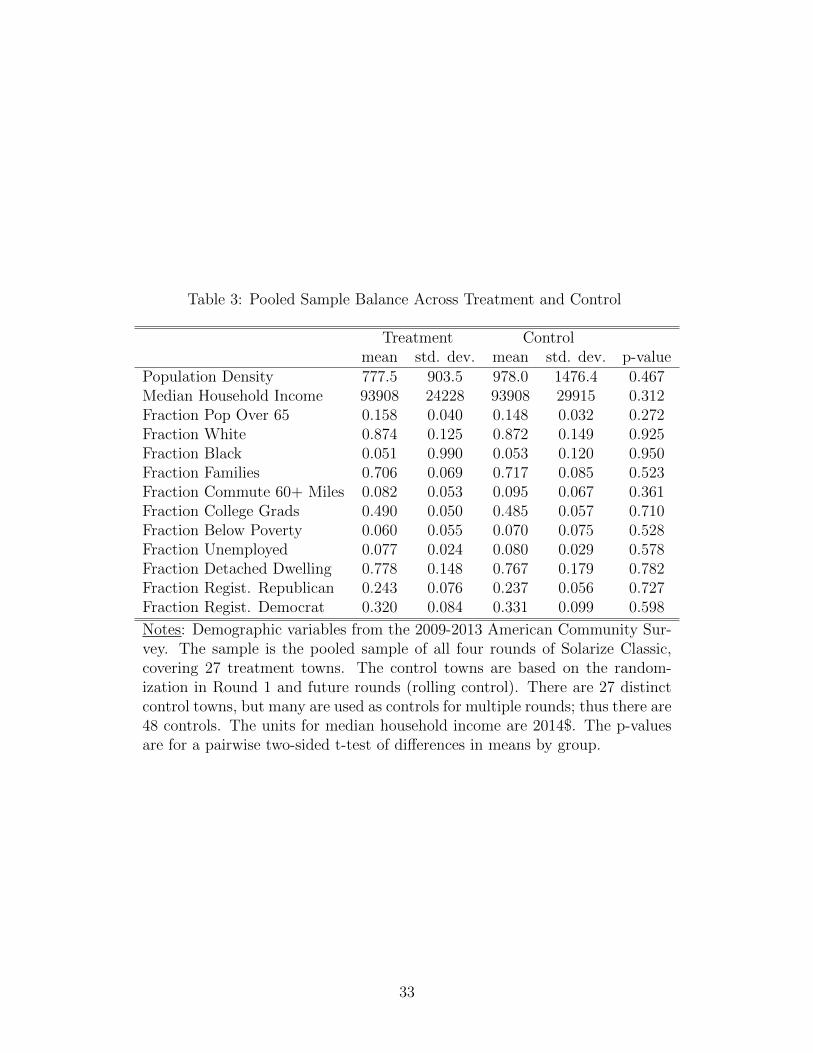
Table 3: Pooled Sample Balance Across Treatment and Control

Treatment Controlmean std. dev. mean std. dev. p-value

Population Density 777.5 903.5 978.0 1476.4 0.467Median Household Income 93908 24228 93908 29915 0.312Fraction Pop Over 65 0.158 0.040 0.148 0.032 0.272Fraction White 0.874 0.125 0.872 0.149 0.925Fraction Black 0.051 0.990 0.053 0.120 0.950Fraction Families 0.706 0.069 0.717 0.085 0.523Fraction Commute 60+ Miles 0.082 0.053 0.095 0.067 0.361Fraction College Grads 0.490 0.050 0.485 0.057 0.710Fraction Below Poverty 0.060 0.055 0.070 0.075 0.528Fraction Unemployed 0.077 0.024 0.080 0.029 0.578Fraction Detached Dwelling 0.778 0.148 0.767 0.179 0.782Fraction Regist. Republican 0.243 0.076 0.237 0.056 0.727Fraction Regist. Democrat 0.320 0.084 0.331 0.099 0.598

Notes: Demographic variables from the 2009-2013 American Community Sur-vey. The sample is the pooled sample of all four rounds of Solarize Classic,covering 27 treatment towns. The control towns are based on the random-ization in Round 1 and future rounds (rolling control). There are 27 distinctcontrol towns, but many are used as controls for multiple rounds; thus there are48 controls. The units for median household income are 2014$. The p-valuesare for a pairwise two-sided t-test of differences in means by group.

33

Table 4: Primary Treatment Effect Results

(1) (2) (3) (4) (5) (6)Round 1 Round 2 Round 3 Round 4 Pooled

random future future future future rand/futureTreatment Effect 2.21*** 2.04*** 1.34*** 0.95*** 1.18*** 1.31***

(0.25) (0.23) (0.17) (0.16) (0.15) (0.13)During Campaign 0.08 0.26*** 0.26*** 0.32*** 1.01*** 0.41***

(0.08) (0.03) (0.04) (0.05) (0.14) (0.05)Constant X X X X X XTown FE X X X X X XR-squared 0.771 0.926 0.923 0.903 0.833 0.892N 882 5292 5250 3808 2737 12677

Number of total towns 9 53 49 33 22 54Number of treated towns 4 4 5 11 7 27Ave. treat. effect per town 53.41 52.18 20.82 15.59 42.91 26.85Ave. installs per treat. town 67.50 67.50 30.20 31.45 81.57 49.55

Notes: Dependent variable is the log odds-ratio of market shares. Unit of observation is town-month. “Random” refers to randomly selected control towns; “future” refers to future selectedtowns as controls. Standard errors clustered on town in parentheses. p < 0.1 (*), p < 0.05(**), p < 0.01 (***).

34

Table 5: Results Including Price

(1) (2) (3) (4) (5) (6)Round 1 Round 2 Round 3 Round 4 Pooled

random future future future future rand/futureTreatment Effect 2.17*** 2.02*** 1.32*** 0.95*** 1.16*** 1.30***

(0.25) (0.23) (0.17) (0.16) (0.15) (0.13)During Campaign 0.03 0.22*** 0.21*** 0.26*** 0.94*** 0.35***

(0.08) (0.03) (0.03) (0.05) (0.13) (0.04)Price Per Watt -0.02*** -0.01*** -0.02*** -0.03*** -0.03*** -0.02***

(0.007) (0.002) (0.002) (0.004) (0.005) (0.003)Constant X X X X X XTown FE X X X X X XR-squared 0.831 0.926 0.924 0.905 0.837 0.894N 882 5292 5250 3808 2737 12677

Number of total towns 9 53 49 33 22 54Number of treated towns 4 4 5 11 7 27Ave. treat. effect per town 53.23 52.09 20.72 15.50 42.61 26.70Ave. installs per treat. town 67.50 67.50 30.20 31.45 81.57 49.55

Notes: Dependent variable is the log odds-ratio of market shares. Unit of observation is town-month. “Random” refers to randomly selected control towns; “future” refers to future selectedtowns as controls. Standard errors clustered on town in parentheses. p < 0.1 (*), p < 0.05(**), p < 0.01 (***).

35

Table 6: IV Results Including Price

(1)Pooled

rand/futureTreatment Effect 1.30***

(0.13)During Campaign 0.36***

(0.06)Price Per Watt -0.02**

(0.01)Constant XTown FE XR-squared 0.894N 12677

Number of total towns 54Number of treated towns 27Ave. treat. effect per town 26.70Ave. installs per treat. town 49.55

Notes: Dependent variable is the logodds-ratio of market shares. The priceper watt is instrumented using the elec-trician wage and roofer wage. Both in-struments are statistically significant atthe 1% level in the first stage with a first-stage F-statistic of 240. Unit of observa-tion is town-month. This estimation usesthe randomly selected control group forround 1 and the future control groups forall other rounds. Standard errors clus-tered on town in parentheses. p < 0.1(*), p < 0.05 (**), p < 0.01 (***).

36

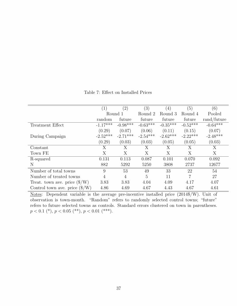
Table 7: Effect on Installed Prices

(1) (2) (3) (4) (5) (6)Round 1 Round 2 Round 3 Round 4 Pooled

random future future future future rand/futureTreatment Effect -1.17*** -0.98*** -0.63*** -0.35*** -0.52*** -0.64***

(0.29) (0.07) (0.06) (0.11) (0.15) (0.07)During Campaign -2.52*** -2.71*** -2.54*** -2.62*** -2.22*** -2.48***

(0.29) (0.03) (0.03) (0.05) (0.05) (0.03)Constant X X X X X XTown FE X X X X X XR-squared 0.131 0.113 0.087 0.101 0.070 0.092N 882 5292 5250 3808 2737 12677

Number of total towns 9 53 49 33 22 54Number of treated towns 4 4 5 11 7 27Treat. town ave. price ($/W) 3.83 3.83 4.04 4.09 4.17 4.07Control town ave. price ($/W) 4.86 4.69 4.67 4.43 4.67 4.61

Notes: Dependent variable is the average pre-incentive installed price (2014$/W). Unit ofobservation is town-month. “Random” refers to randomly selected control towns; “future”refers to future selected towns as controls. Standard errors clustered on town in parentheses.p < 0.1 (*), p < 0.05 (**), p < 0.01 (***).

37

Table 8: Treatment Externalities: Effect on Installations

(1) (2) (3) (4) (5)Round 1 Round 2 Round 3 Round 4 Pooled

Adjacent Town During 0.16** -0.05 0.05 0.17 0.13**(0.07) (0.05) (0.06) (0.12) (0.06)

During Campaign 0.16*** 0.19*** 0.25*** 0.87*** 0.35***(0.02) (0.02) (0.02) (0.05) (0.02)

Constant X X X X XTown FE X X X X XR-squared 0.945 0.942 0.932 0.913 0.930N 16072 16380 15008 14756 61320

Number of total towns 163 155 133 123 164Number of adjacent towns 14 18 29 22 66Ave. treat. effect per adj. town 1.19 2.14Ave. installs per adj. town 3.57 1.94 4.67 18.45 7.54

Notes: Dependent variable is the log odds-ratio of market shares. Unit of observationis town-month. Standard errors clustered on town in parentheses. p < 0.1 (*), p < 0.05(**), p < 0.01 (***).

Table 9: Treatment Externalities: Effect on Prices

(1) (2) (3) (4) (5)Round 1 Round 2 Round 3 Round 4 Pooled

Adjacent Town During -0.19* -0.25*** -0.07 0.01 -0.15***(0.11) (0.06) (0.05) (0.12) (0.03)

During Campaign -2.68*** -2.45*** -2.65*** -2.28*** -2.51***(0.03) (0.02) (0.02) (0.05) (0.01)

Constant X X X X XTown FE X X X X XR-squared 0.108 0.081 0.098 0.067 0.088N 16072 16380 15008 14756 61320

Number of total towns 163 155 133 123 164Number of adjacent towns 14 18 29 22 66Adj. town ave. price ($/W) 4.64 4.55 4.37 4.64 4.52Control town ave. price ($/W) 4.71 4.77 4.42 4.62 4.64

Notes: Dependent variable is the average pre-incentive installed price (2014$/W). Unitof observation is town-month. p < 0.1 (*), p < 0.05 (**), p < 0.01 (***).

38

Table 10: Results for Solarize Randomized Across CT

(1) (2) (3)installs installs prices

Treatment Effect 0.55*** 0.54*** -0.35***(0.13) (0.13) (0.11)

During Campaign 0.91*** 0.84*** -2.26***(0.05) (0.04) (0.02)

Price Per Watt -0.03***(0.003)

Constant X X XTown FE X X XR-squared 0.907 0.910 0.066N 15,960 15,960 15,960

Number of total towns 9 53 49Number of treated towns 4 4 5Ave. treat. effect per town 12.70 12.50Ave. installs per treat. town 39.40 39.40Treat. town ave. price ($/W) 4.30Control town ave. price ($/W) 4.62

Notes: Dependent variable is listed on the column heading; “in-stalls” refers to the log odds-ratio of the market shares. Unit ofobservation is town-month. Standard errors clustered on townin parentheses. p < 0.1 (*), p < 0.05 (**), p < 0.01 (***).

39

Table 11: Connecticut Solar Challenge Results

(1) (2) (3) (4) (5) (6)installs installs prices installs installs prices

Treatment Effect 0.61*** 0.61*** 0.01*** 0.61*** 0.61*** 0.006(0.11) (0.12) (0.07) (0.13) (0.13) (0.07)

During Campaign 0.21 0.17*** -2.54*** 0.24*** 0.19*** -2.55***(0.02) (0.03) (0.03) (0.03) (0.03) (0.03)

Post Treatment Effect 0.49** 0.48** -0.46**(0.23) (0.04) (0.18)

During Post Period 0.50*** 0.45*** -2.67***(0.06) (0.06) (0.05)

Price Per Watt -0.02*** -0.03*** -0.02*** -0.02***(0.003) (0.004) (0.002) (0.003)

Constant X X X X X XTown FE X X X X X XR-squared 0.923 0.924 0.924 0.098 0.915 0.165N 5007 5007 5007 5243 5243 5243

Number of total towns 47 47 47 47 47 47Number of treated towns 3 3 3 3 3 3Ave. treat. effect per town 6.94 6.94 7.07 7.07Post-period ave. treat effect 7.03 7.03Ave. installs per treat. town 11.33 11.33 11.33 11.33Treat. town ave. price ($/W) 4.73 4.73Post-period ave. price ($/W) 4.14Control town ave. price ($/W) 4.66 4.54

Notes: Dependent variable is the log odds-ratio of market shares or prices (2014$/W). Unit ofobservation is town-month. All towns use future (rolling) controls. Standard errors clusteredon town in parentheses. p < 0.1 (*), p < 0.05 (**), p < 0.01 (***).

40

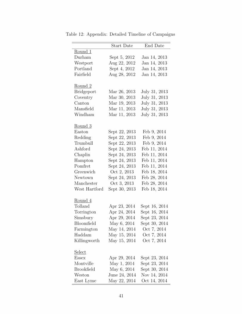
Table 12: Appendix: Detailed Timeline of Campaigns

Start Date End DateRound 1Durham Sept 5, 2012 Jan 14, 2013Westport Aug 22, 2012 Jan 14, 2013Portland Sept 4, 2012 Jan 14, 2013Fairfield Aug 28, 2012 Jan 14, 2013

Round 2Bridgeport Mar 26, 2013 July 31, 2013Coventry Mar 30, 2013 July 31, 2013Canton Mar 19, 2013 July 31, 2013Mansfield Mar 11, 2013 July 31, 2013Windham Mar 11, 2013 July 31, 2013

Round 3Easton Sept 22, 2013 Feb 9, 2014Redding Sept 22, 2013 Feb 9, 2014Trumbull Sept 22, 2013 Feb 9, 2014Ashford Sept 24, 2013 Feb 11, 2014Chaplin Sept 24, 2013 Feb 11, 2014Hampton Sept 24, 2013 Feb 11, 2014Pomfret Sept 24, 2013 Feb 11, 2014Greenwich Oct 2, 2013 Feb 18, 2014Newtown Sept 24, 2013 Feb 28, 2014Manchester Oct 3, 2013 Feb 28, 2014West Hartford Sept 30, 2013 Feb 18, 2014

Round 4Tolland Apr 23, 2014 Sept 16, 2014Torrington Apr 24, 2014 Sept 16, 2014Simsbury Apr 29, 2014 Sept 23, 2014Bloomfield May 6, 2014 Sept 30, 2014Farmington May 14, 2014 Oct 7, 2014Haddam May 15, 2014 Oct 7, 2014Killingworth May 15, 2014 Oct 7, 2014

SelectEssex Apr 29, 2014 Sept 23, 2014Montville May 1, 2014 Sept 23, 2014Brookfield May 6, 2014 Sept 30, 2014Weston June 24, 2014 Nov 14, 2014East Lyme May 22, 2014 Oct 14, 2014

41

Figure 1: Map of Solarize programs in Connecticut in this study.

42

Figure 2: Cumulative installations in Solarize Rounds 1 and 2.

050

100

150

Cum

ulat

ive

Inst

alla

tions

2005w1 2010w1 2015w1Time

Solarize Phase 1 Solarize Phase 2Phase 1 towns Phase 2 towns

Cumulative Number of InstallationsSolarize Classic: Phase 1 and 2

Figure 3: Cumulative installations in Solarize Rounds 3 and 4.

050

100

150

200

Cum

ulat

ive

Inst

alla

tions

2005w1 2010w1 2015w1Time

Solarize Phase 3 Solarize Phase 4Phase 3 towns Phase 4 towns

Cumulative number of InstallationsSolarize Classic: Phase 3 and Phase 4

43

Figure 4: Monthly installations by round.

R1 R2 R3 R4

010

2030

40m

onth

ly a

vera

ge in

stal

ls p

er to

wn

2011m1 2012m1 2013m1 2014m1 2015m1month

Phase 1 Phase 2Phase 3 Phase 4Non-Solarize CEC CT average

Figure 5: Monthly average prices by round.

R1 R2 R3 R4

24

68

10m

onth

ly a

vera

ge p

rice

by to

wn

(201

4$/W

)

2011m1 2012m1 2013m1 2014m1 2015m1month

Round 1 Round 2Round 3 Round 4Non−Solarize CEC CT average

44

Figure 6: Treatment Effects Over Time.

−4

−3

−2

−1

01

23

4

2011m1 2012m1 2013m1 2014m1 2015m1Month

Round 1 Treatment Effect

units in terms of the log−odds ratio

Figure 7: Treatment Effects Over Time.

−4

−3

−2

−1

01

23

4

2011m1 2012m1 2013m1 2014m1 2015m1Month

Round 2 Treatment Effect

units in terms of the log−odds ratio

45

Figure 8: Treatment Effects Over Time.

−4

−3

−2

−1

01

23

4

2011m1 2012m1 2013m1 2014m1 2015m1Month

Round 3 Treatment Effect

units in terms of the log−odds ratio

Figure 9: Treatment Effects Over Time.

−4

−3

−2

−1

01

23

4

2011m1 2012m1 2013m1 2014m1 2015m1Month

Round 4 Treatment Effect

units in terms of the log−odds ratio

46

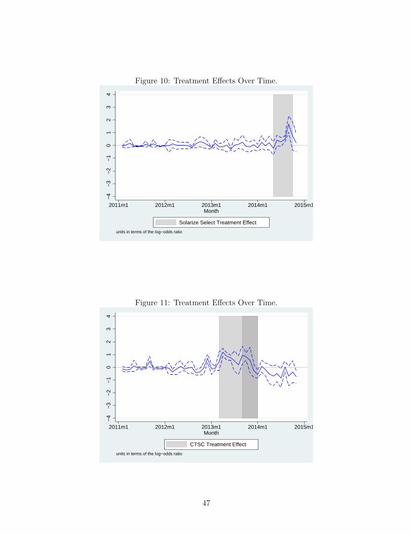
Figure 10: Treatment Effects Over Time.

−4

−3

−2

−1

01

23

4

2011m1 2012m1 2013m1 2014m1 2015m1Month

Solarize Select Treatment Effect

units in terms of the log−odds ratio

Figure 11: Treatment Effects Over Time.

−4

−3

−2

−1

01

23

4

2011m1 2012m1 2013m1 2014m1 2015m1Month

CTSC Treatment Effect

units in terms of the log−odds ratio

47

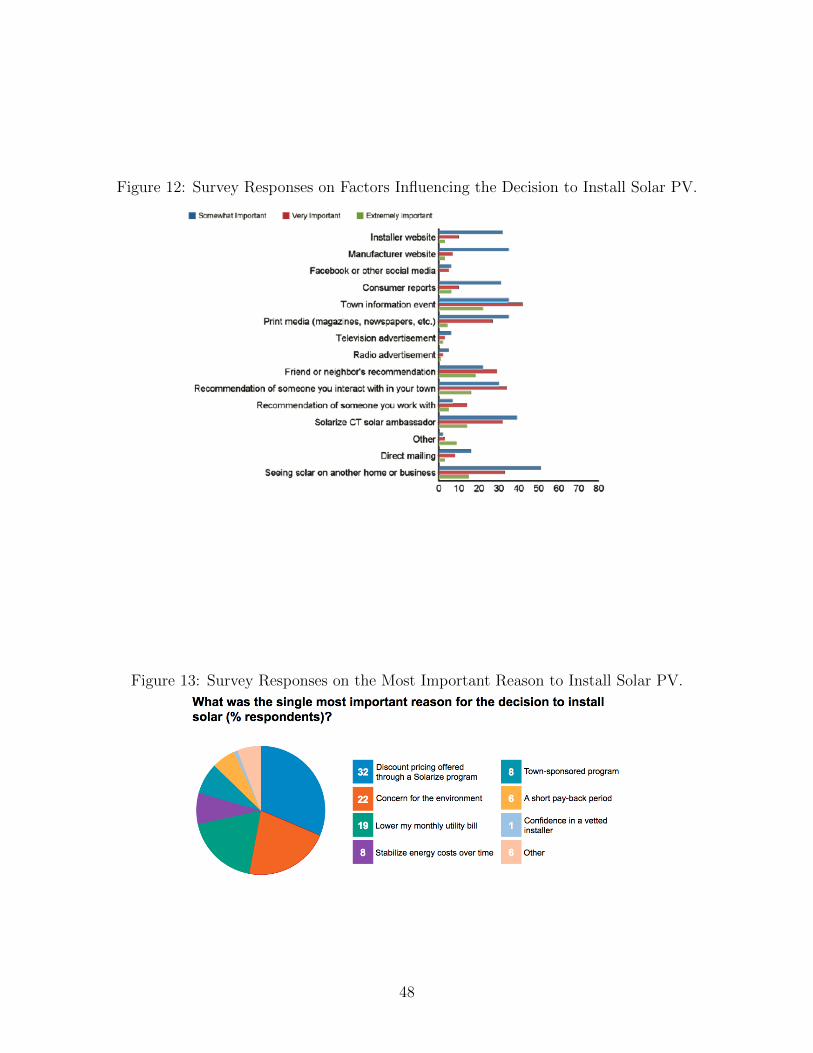
Figure 12: Survey Responses on Factors Influencing the Decision to Install Solar PV.

Figure 13: Survey Responses on the Most Important Reason to Install Solar PV.

48