Social Network Analysis Hemant Gupta , Anurag Das and Manoj Kakarla

{hemantgupta, anuragdas, manojkakarla}@cmail.carleton.ca

Abstract—Network analysis has become an increasingly popular

tool for scholars to deal with the complexity of the

interrelationships between actors of all sorts. The promise of

network analysis is the placement of signs on the relationships

between actors, rather than seeing actors as isolated entities.

Network analysis includes the formulation and solution of

problems that have a network structure; such structure is

captured in a graph. This paper, going to discuss the social

network analysis and how it can be used for media network

analysis using two datasets which involve media network and

media-user network. In this paper we also represent the network

with different methods to make it more understandable. We also

show that how we can use R packages to collect data directly

from the network. This paper helps in a representation of

different types of network.

Keyword- Network Analysis, SNA, igraph

I. INTRODUCTION

Social network analysis (SNA) is the process of

investigating social structures using networks and graph

theory. It characterizes networked structures regarding nodes

(individual actors, people, or things within the network) and

the ties, edges, or links (relationships or interactions) that

connect them. Examples of social structures commonly

visualized through social network analysis include social

media networks, memes spread, friendship and acquaintance

networks, collaboration graphs, kinship, disease transmission,

and sexual relationships. These networks are visualized

through sociograms in which nodes are represented as points

and relationships are represented using lines.

Social network analysis has risen as an important technique

in modern sociology. It has a significant following in

anthropology, biology, demography, communication studies,

economics, geography, history, information science,

organizational studies, political science, social psychology,

development studies, sociolinguistics, and computer science

and is now commonly available as a consumer tool like

NodeXL, TouchGraphSEO, etc.

(Social) Network Analysis has found practical usage in

many domains, although the greatest advances have been

about the study of structures generated by humans. Computer

scientists, for example, have used (and even developed new)

network analysis methods to study web pages, Internet traffic,

information dissemination, etc.

This paper was submitted as the project report of the course titled “Data

Mining” taught by Dr. Shirley E. Mills at Carleton University.

One of example in life sciences is the use of network analysis

to analyze food chains in the ecosystems. Mathematicians and

physicists normally focus on producing new and complex

methods for the study of networks, that is used by anyone, in

any domain where networks are relevant.

Big companies use SNA to study and improve

communication flow in their organization or with their

networks of partners. Customers Law enforcement agencies

with the help of SNA identify criminal and terrorist networks.

With the help of traces of communication that they collect and

then find essential people in these networks. Social Network

Sites like Facebook use simple elements of SNA to identify

and recommend potential friends. This works on friends-of-

friends Civil society organizations which use SNA to uncover

conflicts of interest in hidden connections between

government bodies, lobbies and businesses Network operators

(telephony, cable, mobile).

In this paper, we will discuss literature review in section 2,

and technical background about tools used to represent the

network in section 3. In section 4, we will be discussing the

methodology used to represent the network in different

formats for analysis and section 5 will be about the

conclusion.

II. LITERATURE REVIEW

[1] shows a discussion of social network analysis from

historical studies. It shows the historical, social dynamics from

1204 to 1453 in Byzantium.

Dynamic network analysis (DNA) [2] varies from

traditional social network analysis in that it can handle large

dynamic multi-mode, multi-link networks with varying levels

of uncertainty. An approach to DNA is described that builds

DNA theory through the combined use of multi-agent

modeling, machine learning, and meta-matrix approach to

network representation. In contrast to traditional SNA, DNA

considers the role of the agent regarding processes and not just

position. That is, the agents can do things – communicate,

store information, learn. The links are probabilistic, the

networks multi-colored and multiplex to the extent that the set

of networks combine into one complex system where changes

in one sub-network inform and constrain changes in the

others, often leading to error cascades.

This is a group assignment. Assignees are Hemant Gupta (101062246), Anurag Das (101089268) and Manoj Kakarla (101071887). All group

members are students of Carleton University.

In [3], two different mixed integer linear programming

models (MILP) are applied to a social network dataset, to

compare the optimal results from contrasting models and gain

insight on the applicability of the models on a social network

context.

The objectives of [4] are to check the international trade

relations of the top 20 countries that sell products related to

the production of wind energy and which are the main

products in international trade in this sector. The motivation

for the analysis of this energy matrix stems from the need of

more consistent public policies for production, because the

logistics necessary to reach the end consumer, as this energy

source needs to be installed in places with good intensity

winds, and later transported to the consumer market.

Authors of [5] offer a new approach to the analysis of data

and detection of potential threats in the sphere of public

procurements based on cluster analysis and data mining

techniques.

In [6], authors present an approach to automatically analyze

the Twitter user profiles of a specific community of users. The

locations of users are selected by the user. The proposed

analysis is done by extracting some characteristics of the

collected profiles (of that given community). This analysis

includes the detection of outliers, the clustering of profiles and

their classification. The most important characteristic of the

presented approach is that it can cope with the data of

thousands of Twitter profiles in real-time. Thus, this work is

related to big data in big data analytics.

The purpose of [7] is to identify methods that measure the

skills, expertise, and experience of a job seeker and to

investigate the importance of using social networking data as

input to user modeling that determines the strength of skills to

be used for recommending matching job vacancies.

[8], [9] and [10] are some prestigious conferences on social

network analysis. [11], [12] and [13] are prominent journals

on the same field. [14] is Center for Computational Analysis

of Social and Organizational Systems (CASOS) at Carnegie

Mellon where they address complex real-world issues through

a combined social-science & computer-science approach,

using advanced techniques from network science, text-mining,

and agent-based modeling.

III. TECHNICAL BACKGROUND

A. Definition of a Network

There are several ways of formally defining a network,

depending on the branch of mathematics used[26]. The most

usual and flexible definition [17] is derived from graph theory,

which conceptualizes a social network is conceptualized as a

graph, that is, a set of vertices (or nodes, units, points)

representing social actors or objects and a set of lines

representing one or more social relations among them. A

network, however, is more than a graph because it contains

additional information on the vertices and lines[26].

Characteristics of the social actors, for instance, a person's sex,

age, or income, are represented by discrete or continuous

attributes of the vertices in the network, and the intensity,

frequency, valence, or type of social relation are represented

by line weights, line values, line signs, or line type. Formally,

a network N can be defined as N= (U, L, FU, FL) containing a

graph G= (U, L), which is an ordered pair of a unit or vertex

set U and a line set L, extended with a function FU specifying

a vector of properties of the units (f: U → X) and a function

FL specifying a vector of properties of the lines (f: L → Y).

The set of lines L may be regarded as the union of a set of

undirected edges E and a set of directed arcs A (A E L ∪=).

Each element of E (each edge) is an unordered pair of units u

and v (vertices) from U, that is, e (u: v), and each element a of

A (each arc) is an ordered pair of units u and v(vertices) from

U, that is, a (u: v)[26].

B. Basic Metrices

Some basic metrices [15] to base our analysis on:

1) Connections

Homophily[27]: The extent to which actors form ties with

similar versus dissimilar others. Similarity can be defined by

gender, race, age, occupation, educational achievement, status,

values or any other salient characteristic.

Multiplexity: The number of content-forms contained in a

tie. For example, two people who are friends and also work

together would have a multiplexity of 2. Multiplexity has been

associated with relationship strength.

Mutuality/Reciprocity: The extent to which two actors

reciprocate each other's friendship or other interaction.

Network Closure: A measure of the completeness of

relational triads. An individual's assumption of network

closure (i.e. that their friends are also friends) is called

transitivity. Transitivity is an outcome of the individual or

situational trait of Need for Cognitive Closure.

Propinquity: The tendency for actors to have more ties with

geographically close others.

2) Distributions

Bridge: An individual whose weak ties fill a structural hole,

providing the only link between two individuals or clusters. It

also includes the shortest route when a longer one is

unfeasible due to a high risk of message distortion or delivery

failure.

Centrality: Centrality represents to a group of metrics which

aim to quantify the "importance" (in a variety of senses) of a

node (or group) within a network. Examples of common

methods of measuring "centrality" include betweenness

centrality, closeness centrality, eigenvector centrality, alpha

centrality, and degree centrality.

Density: The proportion of direct ties in a network relative

to the total number possible.

Distance: The minimum number of ties required to connect

two actors, as popularized by Stanley Milgram's small world

experiment and the idea of 'six degrees of separation'.

Structural holes: The absence of ties between two parts of a

network. Finding and exploiting a structural hole can give an

entrepreneur a competitive advantage. This concept was

developed by sociologist Ronald Burt and is sometimes

referred to as an alternate conception of social capital.

Tie Strength: Defined by the linear combination of time,

emotional intensity, intimacy and reciprocity (i.e., mutuality).

Strong ties are associated with homophily, propinquity, and

transitivity, while weak ties are associated with bridges.

3) Segmentation

Groups are identified as 'cliques' if every individual is

directly tied to every other individual, 'social circles' if there is

less stringency of direct contact, which is imprecise, or as

structurally cohesive blocks if precision is wanted.

Clustering coefficient: A measure of the likelihood that two

associates of a node are associates. A higher clustering

coefficient indicates a greater 'cliquishness'.

Cohesion: The degree to which actors are connected

directly to each other by cohesive bonds. Structural cohesion

refers to the minimum number of members who, if removed

from a group, would disconnect the group.

Small World: A small world dis a network that looks almost

random but exhibits a significantly high clustering coefficient

(nodes tend to cluster locally) and a relatively short average

path length (nodes can be reached in a few steps). It is a very

common structure in social networks because of transitivity in

strong social ties and the ability of weak ties to reach across

clusters. Such a network will have many clusters but also

many bridges between clusters that help shorten the average

distance between nodes.

C. Basic Tools

Network analysis software consists of either package based

on graphical user interfaces (GUIs), or packages [17][18] built

for scripting/programming languages.

1) GUI Packages

In general, the GUI packages are easier to learn, while

scripting tools are more powerful and extensible. Widely used,

often open-sourced and well-documented GUI packages

include EgoWeb 2.0 (open source), NetMiner, UCINet, Pajek

(freeware), GUESS, ORA, Cytoscape, Gephi, SocNetV (free

software), Meerkat (SNA), and muxViz (open source).

Private GUI packages directed at business customers include

Arcade Analytics, Idiro SNA Plus, Keyhubs, KeyLines,

KXEN, Keynetiq, Linkurious, OrgAnalytix, Orgnet, and

Polinode.

2) Scripting/Programming Tools

Commonly used and well-documented scripting tools used

for network analysis include: NetMiner with Python scripting

engine, the statnet suite of packages for the R statistical

programming language, igraph, which has packages for R and

Python, muxViz (based on R statistical programming language

and GNU Octave) for the analysis and the visualization of

multilayer networks, the NetworkX library for Python, and the

SNAP package for large-scale network analysis in C++ and

Python. Though difficult to learn, some of these open source

packages are growing much faster regarding functionality and

features than privately maintained software, and extensive

documentation and tutorials are available.

D. Packages

Here, we are using R for SNA and R contains several

packages [16] relevant for social network analysis.

Packages we are using in our analysis:

1) Igraph

igraph is a library and R package for network analysis.

Introduction

The main goals of the igraph library are to provide a set of

data types and functions for 1) pain-free implementation of

graph algorithms, 2) fast handling of large graphs, with

millions of vertices and edges, 3) allowing rapid prototyping

via high-level languages like R.

Igraph graphs[28]

Igraph graphs have a class ‘igraph’. They are printed to the

screen in a special format, here is an example, a ring graph

created using make_ring:

IGRAPH U--- 10 10 -- Ring graph + attr: name (g/c), mutual

(g/x), circular (g/x)

‘IGRAPH' denotes that this is an igraph graph. Then come

four bits that denote the kind of the graph: the first is ‘U' for

undirected and ‘D' for directed graphs. The second is ‘N'

named graph (i.e., if the graph has the ‘name' vertex attribute

set). The third is ‘W' for weighted graphs (i.e. if the ‘weight'

edge attribute is set). The fourth is ‘B' for bipartite graphs (i.e.,

if the ‘type' vertex attribute is set).

Then come two numbers, the number of vertices and the

number of edges in the graph, and after a double dash, the

name of the graph (the ‘name’ graph attribute) is printed if

present. The second line is optional, and it contains all the

attributes of the graph. This graph has a ‘name’ graph

attribute, of type character, and two other graph attributes

called ‘mutual’ and ‘circular’, of a complex type. A complex

type is simply anything that is not numeric or character.

If you want to see the edges of the graph as well, then use the

print_all function:

> print_all(g)

IGRAPH badcafe U--- 10 10 -- Ring graph + attr: name (g/c),

mutual (g/x), circular (g/x) + edges:

[1] 1-- 2 2-- 3 3-- 4 4-- 5 5-- 6 6-- 7 7-- 8 8-- 9 9--10 1—10

Creating graphs[29]

There are many functions in igraph for creating graphs, both

deterministic and stochastic; stochastic graph constructors are

called ‘games’.

To create small graphs with a given structure probably the

graph_from_literal function is easiest. It uses R's formula

interface; its manual page contains many examples. Another

option is the graph, which takes numeric vertex ids directly.

graph.atlas creates the graph from the Graph Atlas,

make_graph can create some special graphs[28].

To create graphs from field data, graph_from_edgelist,

graph_from_data_frame, and graph_from_adjacency_matrix

are probably the best choices.

The igraph package[28] includes some classic random

graphs like the Erdos-Renyi GNP and GNM graphs

(sample_gnp, sample_gnm) and some recent popular models,

like preferential attachment (sample_pa) and the small-world

model (sample_smallworld).

Vertex and edge IDs

Vertices and edges have numerical vertex ids in igraph. Vertex

ids are always consecutive, and they start with one. i.e., for a

graph with n vertices, the vertex ids are between 1 and n. If

some operation changes the number of vertices in the graphs,

e.g., a subgraph is created via induced_subgraph, then the

vertices are renumbered to satisfy these criteria[28].

The same is true for the edges as well, edge ids are always

between one and m, the total number of edges in the graph. It

is often desirable to follow vertices along some graph

operations, and vertex ids don't allow this because of the

renumbering. The solution is to assign attributes to the

vertices. These are kept by all operations, if possible.

Attributes

In igraph it is possible to assign attributes to the vertices or

edges of a graph, or to the graph itself. igraph provides

flexible constructs for selecting a set of vertices or edges

based on their attribute values.

Some vertex/edge/graph attributes are treated specially[30].

One of them is the ‘name' attribute. This is used for printing

the graph instead of the numerical ids, if it exists. Vertex

names can also be used to specify a vector or set of vertices, in

all igraph functions. E.g. degree has a v argument that gives

the vertices for which the degree is calculated. This argument

can be given as a character vector of vertex names.

Edges can also have a ‘name' attribute, and this is treated

specially as well. Just like for vertices, edges can also be

selected based on their names, e.g., in the delete_edges and

other functions. Vertex names can also be used to select edges.

The form ‘from-to', where ‘from' and ‘to' are vertex names,

select a single, possibly directed, edge going from ‘from' to

‘to'. The two forms can also be mixed in the same edge

selector.

Attribute values can be set to any R object but note that

storing the graph in some file formats might result from the

loss of complex attribute values. All attribute values are

preserved if you use to save and load to store/retrieve your

graphs.

Visualization

igraph provides three different ways for visualization. The

first is the plot.igraph function. (You don't need to write

plot.igraph, the plot is enough. This function uses regular R

graphics and can be used with any R device.

The second function is tkplot, which uses a Tk GUI for

basic interactive graph manipulation. Tk is quite resourced

hungry, so it is not recommended to use on large graphs.

The third way requires the rgl package and uses OpenGL.

2) sna

sna is a package containing a range of tools for social

network analysis. Supported functionality includes node and

graph-level indices, structural distance and covariance

methods, structural equivalence detection, p* modeling,

random graph generation, and 2D/3D network visualization

(among other things). Network data for sna routines can (except as noted

otherwise) appear in any of the following forms:

● adjacency matrices (dimension N x N)

● arrays of adjacency matrices, aka “graph stacks”

(dimension m x N x N)

● sna edge lists

● sparse matrix objects (from the SparseM package)

● network objects (from the network package)

● lists of adjacency matrices/arrays, sparse matrices,

and/or network objects.

Within the package documentation, the term "graph" is used

generically to refer to any or all of the above (with multiple

graphs being referred to as a "graph stack"). The usage of

sparse matrix objects requires that the SparseM package is

installed. In general, sna routines attempt to make intelligent

decisions regarding the processing of multiple graphs, but

common sense is always advised; certain functions, in

particular, have more specific data requirements. Calling sna

functions with inappropriate input data can produce

"interesting" results.

One special data type supported by the sna package (as of

version 2.0) is the sna edgelist. This is a simple data format

that is well-suited to representing large, sparse graphs. An sna

edgelist is a three-column matrix, containing (respectively)

senders, receivers, and values for each edge in the graph.

(Unvalued edges should have a value of 1.) Note that this form

is invariant to the number of edges in the graph: if there are no

edges, then the edgelist is a degenerate matrix of dimension 0

by 3. Edgelists for undirected graphs should be coded as fully

mutual digraphs (as would be the case with an adjacency

matrix), with two edges per dyad (one (i,j) edge, and one (j,i)

edge). Graph size for an sna edgelist matrix is indicated by a

mandatory numeric attribute, named "n". Vertex names may

be optionally specified by a vector-valued attribute named

"vnames". In the case of two-mode data (i.e., data with an

enforced bipartition), it is possible to indicate this status via

the optional "bipartite" attribute. Vertices in a two-mode

edgelist should be grouped in mode order, with "n" equal to

the total number of vertices (across both modes) and

"bipartite" equal to the number of vertices in the first mode.

Direct creation of sna edgelists can be performed by

creating a three-column matrix and using the attr function to

create the required "n" attribute. Alternately, the function

as.edgelist.sna can be used to coerce data in any of the above

forms to an sna edgelist. By turns, the function

as.sociomatrix.sna can be used to convert any of these data

types to adjacency matrix form.

Some functions in the package-

add.isolates -Add Isolates to a Graph

as.edgelist.sna -sna Coercion Functions

betweenness - Compute the Betweenness Centrality

Scores of Network Positions

blockmodel - Generate Blockmodels Based on

Partitions of Network Positions

blockmodel.expand - Generate a Graph (or Stack)

Blockmodel- - Using Particular Expansion Rules

bn - Fit a Biased Net Model

bonpow - Find Bonacich Power Centrality Scores

of Network Positions

brokerage - Perform a Gould-Fernandez Brokerage

Analysis

centralgraph -Find the Central Graph of a Labeled

Graph Stack

centralization - Find the Centralization of a Given

Network, for Some Measure of

Centrality

clique.census - Compute Cycle Census Information

closeness - Compute the Closeness Centrality

Scores of Network Positions

gplot - Two-Dimensional Visualization of

Graphs

gplot.arrow - Add Arrows or Segments to a Plot

gplot.layout - Vertex Layout Functions for gplot

gplot.loop - Add Loops to a Plot

gplot.target - Display a Graph in Target Diagram

Form

gplot.vertex - Add Vertices to a Plot

gplot3d - Three-Dimensional Visualization of

Graphs

gplot3d.arrow - Add Arrows a Three-Dimensional Plot

gplot3d.layout - Vertex Layout Functions for gplot3d

gplot3d.loop - Add Loops to a Three-Dimensional Plot

3) The Network Dynamic Temporal Visualization (ndtv)

package

Construct visualizations such as timelines and animated

movies of networkDynamic objects to show changes in

structure and attributes over time.

Details

Uses network objects with dynamics encoded using

networkDynamic.

Key features:

● Compute a dynamic layout using compute.animation.

● Render it as a movie using render.animation.

● Render animations to a web page using

render.d3movie

● Plot multiple 'stills' of a movie with filmstrip

● Plot a timeline of edge and vertex activity with

timeline

● Plot network geodesic proximities as a stream graph

with proximity.timeline

4) Other Packages

PAFit can analyse the evolution of complex networks by

estimating preferential attachment and node fitness;

tnet performs analysis of weighted networks, two-mode

networks, and longitudinal networks.

ergm is a set of tools to analyze and simulate networks based

on exponential random graph models exponential random

graph models;

Bergm provides tools for Bayesian analysis for exponential

random graph models;

hergm implements hierarchical exponential random graph

models;

RSiena allows the analyses of the evolution of social networks

using dynamic actor-oriented models;

latentnet has functions for network latent position and cluster

models;

degreenet provides tools for statistical modeling of network

degree distributions;

networksis provides tools for simulating bipartite networks

with fixed marginals; multiplex offers tools for the analysis of

multiple social networks with algebra.

netdiffuseR was designed for the analysis of network diffusion

of innovations (and diffusion in general); bipartite provides

functions to visualise and calculate indices used to describe

bipartite graphs. It focuses on webs, i.e., ecological networks.

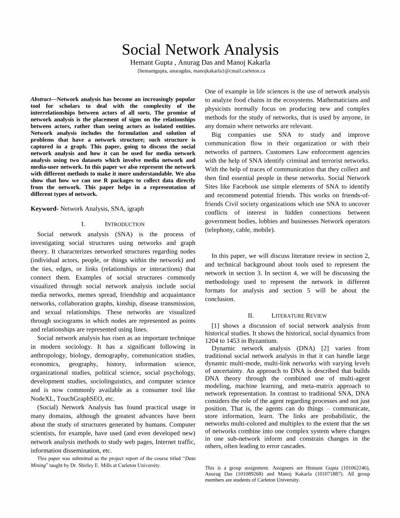
E. Network Visualization

Visual representation of social networks is important to

understand the network data and convey the result of the

analysis. Numerous methods [18][19] of visualization for data

produced by social network analysis have been presented.

Many of the analytic software have modules for network

visualization. Exploration of the data is done through

displaying nodes and ties in various layouts, and attributing

colors, size and other advanced properties to nodes.

Visual representations of networks may be a powerful

method for conveying complex information, but care should

be taken in interpreting node and graph properties from visual

displays alone, as they may misrepresent structural properties

better captured through quantitative analyses.

Figure 1: Network visualization goals

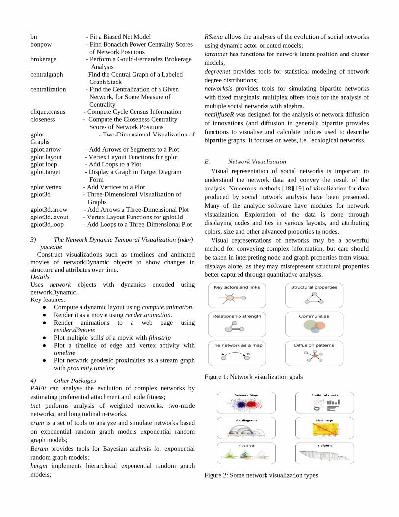
Figure 2: Some network visualization types

Network maps are far from the only visualization available for

graphs - other network representation formats, and even

simple charts of key characteristics, may be more appropriate

in some cases.

In network maps, as in other visualization formats, we have

several key elements that control the outcome. The major ones

are color, size, shape, and position.

Figure 3: Network visualization controls

Modern graph layouts are optimized for speed and aesthetics.

They seek to minimize overlaps and edge crossing and ensure

similar edge length across the graph.

Figure 4: Layout aesthetics

IV. METHODOLOGY

Now we are going to analyze two different types of dataset.

A. First Dataset

It contains two different files Media-Edges.csv and Media-

Nodes.csv. For our analysis, we took 17 different types of

media elements. Media-Nodes.csv file contains the

representation id of the nodes and with their corresponding

real names and the number of audiences attached to that media

type, i.e., Newspaper, TV, online.

Figure 5: Part of Dataset Media-Nodes.csv

Media-Edges.csv contains the links between two media ids

and how they are linked i.e. hyperlink or mention.

Figure 6: Part of Dataset Media-Edges.csv

B. Second Dataset

It contains two different files Media-Edges-User.csv and

Media-Nodes-User.csv. For our analysis, we tool ten different

type of media and 20 users. Media-Edges-User.csv contains

the links between media id and the user id. If a user watches a

certain type of media, it is represented as 1.

Figure 7: Part of Dataset Media-Edges-User.csv

Media-Nodes-User.csv file contains the representation id of

the nodes and with their corresponding real names and the

number of audiences attached to that media type, i.e.,

Newspaper, TV, online. Also present is the user id and their

corresponding names.

Figure 8: Part of Dataset Media-Nodes-User.csv

C. Cleaning Dataset

There are many links than unique from-to combinations.

Here we case in the data where there are multiple links

between the same two nodes. Collapse all links of the same

type between the same two nodes by summing their weights,

using aggregate () by “from”, “to”, & “type”:

D. Network Visualization with igraph

Convert the raw data to the network object. Here we use

igraph's graph.data.frame function, which takes two data

frames: d and vertices[20][21][22].

● d describes the edges of the network. Its first two

columns are the IDs of the source and the target node

for each edge. The following columns are edge

attributes (weight, type, label, or anything else).

● Vertices start with a column of node IDs. Any

following columns are interpreted as node attributes.

Figure 9: Network Representation of Media using Node id and

links, i.e., edges

Figure 10: Network Representation of Media using Node id

and links, i.e., edges with reduced arrow size

Now as we have our igraph network object, we make a first

attempt to plot it. With the help of below graph, we can see the

connections between different node ids and can comment

whether it's unidirectional or bidirectional.

In the next step, we remove the loops in the network and

adjust the arrow size to look better. With the help of this, we

can see the connection between node id properly.

Now as we know, we are not proper clear about the graph as

these node ids did not give proper information. Let's use the

corresponding names for each node id and plot the network.

By using names, graph gives a better understanding of

network, and becomes more readable.

Figure 11: Network Representation of Media using names

Another way to plot a network is to set attributes to add them

to the igraph object. Represent network nodes with colors

based on the type of media, and size them based on degree

centrality (more links -> larger node) We will also change the

width of the edges based on their weight. With the help of this,

we can conclude that television nodes have high degree

centrality due to their large size and newspaper has higher

weights as they have more width on their edges.

Figure 12: Network Representation of Media based on degree

centrality and weights

E. Network Layout

Fruchterman-Reingold is one of the important used force-

directed layout algorithms.

Some parameters can set for this layout include are the area

(the default is the square of # nodes) and repulserad

(cancellation radius for the repulsion - the area multiplied by #

nodes). Both parameters affect the spacing of the plot - play

with them until you like the results.

Figure 13(A): Different Network layout available in igraph

for the Dataset 1.

Figure 13(B): Different Network layout available in igraph

for the Dataset 1.

Figure 13(C): Different Network layout available in igraph

for the Dataset 1.

Set the “weight” parameter which increases the attraction

forces among nodes connected by heavier edges. All network

layout available in igraph for the Dataset 1.

As we know that network plot is still not that much helpful,

we cannot examine the network properly as the link is so

dense. We took an approach to see if we can sparsify the

network, keeping only the most important ties and remove the

rest. For the Current analyzing dataset, we'll only keep ones

that have the weight higher than the mean for the network.

This makes the analysis easier.

Figure 14: Network With links whose weight higher than

mean

Another way is to plot the two tie types (hyperlink & mention)

separately. In this representation, dark color represent

hyperlink and slate-grey represent mention. We can also

represent them separately to understand the relationship of

nodes with hyperlink and mention respectively.

Figure 15: Network Representation using hyperlink and

mention

Figure 16: Network Representation using Hyperlink and

Mention separately

F. Highlighting specific nodes, links, and paths

focusing the visualization on a node or a group of nodes. In

our dataset media network, we can examine the spread of

information from focal actors. For instance, let's represent the

distance from the NYT. The shortest.paths function (as its

name indicates) returns a matrix of shortest paths between

nodes in the network. With this representation, we can get the

first-degree neighbors, second degree and so on of NYT and

with the help of this, we can find the multipoint relay nodes

for NYT to cover the whole network.

Figure 17: Network representation of node NYT and its

neighbors

We can also plot the shortest path between two nodes and with

the help this we can find the number of hopes required to

reach from one node to another.

Figure 18: Network Representation of two nodes shortest path

G. More ways to represent the network

Sometimes Normal plots like the heat wave and simple

graph are more informative in case of network analysis.

Heatmap of the network matrix. A simple graph is based on

what properties of the network or its nodes and edges are most

important.

Figure 19: Heatmap of Network Matrix of Dataset 1

Figure 20: Simple graph of Network Matrix of Dataset 1

H. Plotting two-mode networks with igraph

Two-mode or bipartite graphs have two different types of

actors and links that go across, but not within each type. Our

second Media-User Dataset is a network of that kind,

examining links between news sources and their consumers.

As you will see below, this time the edges of the network are

in a matrix format. We can read those into a graph object

using graph.incidence.

As with one-mode networks, we modify the network object

to include the visual properties which will be used by default

while plotting the network. Note that this time we will change

the shape of the nodes-media outlets be squares, and their

users are circles. This shows the relationship between media

nodes and user attached to it[24][25].

Figure 21: Network Representation of Dataset 2 with Media

and User.

We can also use text as nodes which may be helpful at times.

And sometimes we can also experiment with the use of images

as nodes. To do this, you will need the png library to look

more interactive. Instead of using the nodes of different shapes

we can use the names of media types and usernames. We can

also use the images to represent media and user. It gives the

good visualization and easy for understanding to people who

are not from the technical background.

Figure 22(A): Representation of Two mode network with

names and image icons.

Figure 22(B): Representation of Two mode network with

names and image icons.

I. Reading Dataset using R packages.

We can also directly read the data from the network using few

of the R packages like twitteR. It gives us an interface to the

Twitter web API. Main Functionality of the API is supported,

using a bias towards API calls which are more useful in data

analysis.

The first thing needs to do is download the twitteR package

and make it available in your R session.

library(twitteR)Now on the Twitter side, you need to do a

few things to get setup. Need to have a twitter account and

also need to have a mobile number as part of this account.

Figure 23: Twitter Login Page

Now go to https://apps.twitter.com and sign on with your

twitter account.

Figure 24: Twitter Page after Successful login

Once signed in, able to see the following screen, and simply

click on the button that says "Create New App."

Figure 25: Twitter Page with Create New App Option

Once click on the "Create New App" button, system go to the

Create an Application screen. There are three fields, a click

box and a button which we need to click on this page. The

three fields are Name, Description, and Website. Name of the

application must be unique. The description needs to be at

least ten characters long and put on a website. If do not have

one, use https://bigcomputing.blogspot.com. Now click the

"Yes, I agree" box for the license agreement and click the

"Create your Twitter application."

Figure 26: Twitter Create Application Page

Once successfully create an application, the system now will

be taken to an application page. Once there click on "key and

access token" tab. From that page going to need four things.

1. Consumer Key (API Key)

2. Consumer Secret (API Secret)

Click the "Create my access token" button.

3. Access Token

4. Access Token Secret

Now re-open your R session and enter the following code

using those four pieces of information.

consumer_key <- “your_consumer_key”

consumer_secret <- “your_consumer_secret”

access_token <- “your_access_token”

access_secret <- “your_access_secret”

setup_twitter_oauth(consumer_key, consumer_secret,

access_token, access_secret)

Now set up on the Twitter side and the R side is successful

and should be ready to go.

Please see the appendix 2 for R code for fetching the twitter

data.

V. CONCLUSION AND FUTURE WORK

SNA is a unique representation of how society works. Instead

of focusing on individuals and their attributes, or on

macroscopic social structures, it centers on relations between

individuals, groups, or social institutions. Studying society

from a network point of view is to analyze individuals as a

part of a network of relations and which seek explanations for

social behavior in the structure of these networks. An idea

that networks of relations are important in case of social

science is widespread availability of data and growth in computing and methodology have made it much easier now to

apply SNA to a range of problems.

CONTRIBUTION

Hemant Gupta (101062246) was the primary programmer. He

also wrote methodology, abstract and conclusion. Anurag Das

(101089268) was the secondary programmer. He wrote the

literature review and integrated all work into a single file.

Manoj Kakarla (101071887) wrote the introduction and

technical work.

REFERENCES

[1] Web.archive.org. (2018). Complex Byzantium: a new analysis of the

fatal crisis of Medieval Europe´s most ancient Empire, 1204-1453. [2] Casos.cs.cmu.edu. (2018). [online] Available at:

http://www.casos.cs.cmu.edu/publications/protected/2000-

2004/2003-2004/carley_2003_dynamicnetwork.pdf [3] H. Pirim, "Mathematical programming for social network analysis,"

2017 IEEE International Conference on Big Data (Big Data), Boston, MA, 2017, pp. 2085-2088.

[4] F. G. Basso, G. S. Porto and S. K. Junior, "International Trade

Relations of Products for Wind Energy Production: A Study from the

Dynamic Social Network Analysis (DSNA)," 2017 Portland

International Conference on Management of Engineering and

Technology (PICMET), Portland, OR, 2017, pp. 1-18. [5] D. V. I., M. N. V. and B. M. I, "Adaptation of Cluster Analysis

Methods in Respect to Vector Space of Social Network Analysis

Indicators for Revealing Suspicious Government Contracts," 2017 5th International Conference on Future Internet of Things and Cloud

Workshops (FiCloudW), Prague, 2017, pp. 57-62. [6] J. A. Iglesias, A. García-Cuerva, A. Ledezma and A. Sanchis, "Social

network analysis: Evolving Twitter mining," 2016 IEEE

International Conference on Systems, Man, and Cybernetics (SMC), Budapest, 2016, pp. 001809-001814.

[7] S. Chala and M. Fathi, "Job seeker to vacancy matching using social

network analysis," 2017 IEEE International Conference on Industrial

Technology (ICIT), Toronto, ON, 2017, pp. 1250-1255. [8] Insna.org. (2018). Sunbelt Archives. [online] Available at:

http://www.insna.org/archives.html

[9] Asonam.cpsc.ucalgary.ca. (2018). ASONAM 2018 | Home Page.

[online] Available at: http://asonam.cpsc.ucalgary.ca/2018 [10] Graphdrawing.org. (2018). GD symposia. [online] Available at:

http://www.graphdrawing.org/symposia.html [11] Applied Network Science. [online] Applied Network Science.

Available at: https://appliednetsci.springeropen.com. [12] Link.springer.com. (2018). Social Network Analysis and Mining -

Springer. [online] Available at: https://link.springer.com/journal/13278 [Accessed 29 Mar. 2018].

[13] Ees.elsevier.com. (2018). Elsevier Editorial SystemTM. [online]

Available at: https://ees.elsevier.com/son/default.asp. [14] Casos.cs.cmu.edu. (2018). Homepage | CASOS. [online] Available

at: http://www.casos.cs.cmu.edu [15] 1.

https://wiki.nus.edu.sg/download/attachments/57742900/Social%20Network%20Analysis.pdf

[16] J. O. Abe, H. A. Mantar and A. G. Yayimli, "k -Maximally Disjoint

Path Routing Algorithms for SDN," 2015 International Conference

on Cyber-Enabled Distributed Computing and Knowledge Discovery,

Xi'an, 2015, pp. 499-508. [17] C. Gao, W. Zhang, J. Tang, R. K. Sinha and K. N. Oikonomou,

"DEMUR: Dependable Multipath Routing in Software Defined Networking for ISP Backbone," GLOBECOM 2017 - 2017 IEEE

Global Communications Conference, Singapore, 2017, pp. 1-6. [18] F. Yaghoubi, M. Furdek, A. Rostami, P. Öhlén and L. Wosinska,

"Consistency-aware Weather Disruption-tolerant Routing in SDN-based Wireless Mesh Networks," in IEEE Transactions on Network

and Service Management, vol. PP, no. 99, pp. 1-1. [19] M. Wang, J. Liu, J. Mao, H. Cheng, J. Chen and C. Qi,

"RouteGuardian: Constructing secure routing paths in software-

defined networking," in Tsinghua Science and Technology, vol. 22, no. 4, pp. 400-412, Aug. 2017.

[20] Zaphiris, Panayiotis & Ang, Chee Siang. (2009). Introduction to

Social Network Analysis (Tutorial). [21] Igraph.org. (2018). Tutorial. [online] Available at:

http://igraph.org/python/doc/tutorial/tutorial.html [22] Rstudio-pubs-static.s3.amazonaws.com. (2018). iGraph tutorial.

Available at: https://rstudio-pubs-

static.s3.amazonaws.com/74248_3bd99f966ed94a91b36d39d8f21e3dc3.html

[23] YouTube. (2018). Tutorial 4 Social Network Analysis. [online]

Available at: https://www.youtube.com/watch?v=d6bi0QTaX5Y [24] Personal.psu.edu. (2018). R for networks: A short tutorial. [online]

Available at: http://personal.psu.edu/drh20/Rnetworks [25] Sadler, J. (2018). Introduction to Network Analysis with R. [online]

Jesse Sadler. Available at:

https://www.jessesadler.com/post/network-analysis-with-r [26] Eolss.net. (2018). [online] Available at:

http://www.eolss.net/Sample-Chapters/C04/E6-99A-16.pdf

[27] Quizlet. (2018). DSS final. Flashcards | Quizlet. [online] Available

at: https://quizlet.com/47002694/dss-final-flash-cards

[28] Igraph.org. (2018). igraph R manual pages. [online] Available at:

http://igraph.org/r/doc/aaa-igraph-package.html

[29] Rdocumentation.org. (2018). igraph-package function | R

Documentation. [online] Available at:

https://www.rdocumentation.org/packages/igraph/versions/1.1.2/topics/igraph-package

[30] Files.meetup.com. (2018). [online] Available at:

http://files.meetup.com/3576292/networks%20in%20R%20using%20

igraph.pdf.

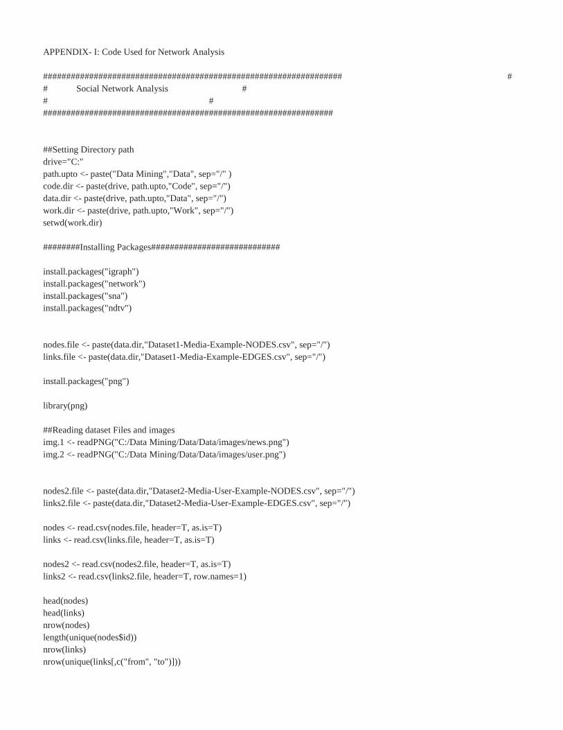
APPENDIX- I: Code Used for Network Analysis

################################################################# #

# Social Network Analysis #

# #

###############################################################

##Setting Directory path

drive="C:"

path.upto <- paste("Data Mining","Data", sep="/" )

code.dir <- paste(drive, path.upto,"Code", sep="/")

data.dir <- paste(drive, path.upto,"Data", sep="/")

work.dir <- paste(drive, path.upto,"Work", sep="/")

setwd(work.dir)

########Installing Packages############################

install.packages("igraph")

install.packages("network")

install.packages("sna")

install.packages("ndtv")

nodes.file <- paste(data.dir,"Dataset1-Media-Example-NODES.csv", sep="/")

links.file <- paste(data.dir,"Dataset1-Media-Example-EDGES.csv", sep="/")

install.packages("png")

library(png)

##Reading dataset Files and images

img.1 <- readPNG("C:/Data Mining/Data/Data/images/news.png")

img.2 <- readPNG("C:/Data Mining/Data/Data/images/user.png")

nodes2.file <- paste(data.dir,"Dataset2-Media-User-Example-NODES.csv", sep="/")

links2.file <- paste(data.dir,"Dataset2-Media-User-Example-EDGES.csv", sep="/")

nodes <- read.csv(nodes.file, header=T, as.is=T)

links <- read.csv(links.file, header=T, as.is=T)

nodes2 <- read.csv(nodes2.file, header=T, as.is=T)

links2 <- read.csv(links2.file, header=T, row.names=1)

head(nodes)

head(links)

nrow(nodes)

length(unique(nodes$id))

nrow(links)

nrow(unique(links[,c("from", "to")]))

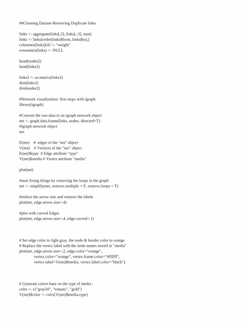
##Cleaning Dataset-Removing Duplicate links

links <- aggregate(links[,3], links[,-3], sum)

links <- links[order(links$from, links$to),]

colnames(links)[4] <- "weight"

rownames(links) <- NULL

head(nodes2)

head(links2)

links2 <- as.matrix(links2)

dim(links2)

dim(nodes2)

#Network visualization: first steps with igraph

library(igraph)

#Convert the raw data to an igraph network object

net <- graph.data.frame(links, nodes, directed=T)

#igraph network object

net

E(net) # edges of the "net" object

V(net) # Vertices of the "net" object

E(net)$type # Edge attribute "type"

V(net)$media # Vertex attribute "media"

plot(net)

#start fixing things by removing the loops in the graph

net <- simplify(net, remove.multiple = F, remove.loops = T)

#reduce the arrow size and remove the labels

plot(net, edge.arrow.size=.4)

#plot with curved Edges

plot(net, edge.arrow.size=.4, edge.curved=.1)

# Set edge color to light gray, the node & border color to orange

# Replace the vertex label with the node names stored in "media"

plot(net, edge.arrow.size=.2, edge.color="orange",

vertex.color="orange", vertex.frame.color="#ffffff",

vertex.label=V(net)$media, vertex.label.color="black")

# Generate colors base on the type of media :

colrs <- c("gray50", "tomato", "gold")

V(net)$color <- colrs[V(net)$media.type]

# Compute node degrees (i.e. links) and using it to modify node size

deg <- degree(net, mode="all")

V(net)$size <- deg*3

# We could use the audience size value also

V(net)$size <- V(net)$audience.size*0.6

# Labels are currently node IDs.

# Setting them to NA will render no labels:

V(net)$label <- NA

# Modify edge width based on weight:

E(net)$width <- E(net)$weight/6

#Modify arrow size and edge color:

E(net)$arrow.size <- .2

E(net)$edge.color <- "gray80"

E(net)$width <- 1+E(net)$weight/12

plot(net)

# Set edge color to light gray, the node & border color to orange

# Replace the vertex label with the node names stored in "media"

plot(net, edge.arrow.size=.2, edge.color="orange",

vertex.color="orange", vertex.frame.color="#ffffff",

vertex.label=V(net)$media, vertex.label.color="black")

#Add legend explaining the meaning of the colors

plot(net)

legend(x=-1.5, y=-1.1, c("Newspaper","Television", "Online News"), pch=21,

col="#777777", pt.bg=colrs, pt.cex=2, cex=.8, bty="n", ncol=1)

#plotting only labels of the nodes

plot(net, vertex.shape="none", vertex.label=V(net)$media,

vertex.label.font=2, vertex.label.color="gray40",

vertex.label.cex=.7, edge.color="gray85")

#Color the edges of graph based on their source node color.

#Get the starting node for each edge with get.edges

edge.start <- get.edges(net, 1:ecount(net))[,1]

edge.col <- V(net)$color[edge.start]

plot(net, edge.color=edge.col, edge.curved=.1)

#layout igraph uses by default are called layout.auto.

#It automatically selects an appropriate layout algorithm

#based on the properties (size and connectedness) of the graph.

#Now look at all available layouts in igraph

layouts <- grep("^layout\\.", ls("package:igraph"), value=TRUE)

# Remove layouts which are not apply to our graph.

layouts <- layouts[!grepl("bipartite|merge|norm|sugiyama", layouts)]

par(mfrow=c(3,3))

for (layout in layouts) {

print(layout)

l <- do.call(layout, list(net))

plot(net, edge.arrow.mode=0, layout=l, main=layout) }

dev.off()

#Analysis of the nodes keeping important one and removing rest

hist(links$weight)

mean(links$weight)

sd(links$weight)

#keep ones that have weight higher than the mean for the network

cut.off <- mean(links$weight)

net.sp <- delete.edges(net, E(net)[weight<cut.off])

l <- layout.fruchterman.reingold(net.sp, repulserad=vcount(net)^2.1)

plot(net.sp, layout=l)

#plot the two tie types (hyperlink & mention) separately

E(net)$width <- 1.5

plot(net, edge.color=c("dark red", "slategrey")[(E(net)$type=="hyperlink")+1],

vertex.color="gray40", layout=layout.circle)

net.m <- net - E(net)[E(net)$type=="hyperlink"] # another way to delete edges

net.h <- net - E(net)[E(net)$type=="mention"]

par(mfrow=c(1,2))

plot(net.h, vertex.color="orange", main="Tie: Hyperlink")

plot(net.m, vertex.color="lightsteelblue2", main="Tie: Mention")

l <- layout.fruchterman.reingold(net)

plot(net.h, vertex.color="orange", layout=l, main="Tie: Hyperlink")

plot(net.m, vertex.color="lightsteelblue2", layout=l, main="Tie: Mention")

#dev.off()

#make the network map more useful by showing the communities within it

V(net)$community <- optimal.community(net)$membership

colrs <- adjustcolor( c("gray50", "tomato", "gold", "yellowgreen"), alpha=.6)

plot(net, vertex.color=colrs[V(net)$community])

#Highlighting specific nodes or links

#1. represent distance from the NYT

dist.from.NYT <- shortest.paths(net, algorithm="unweighted")[1,]

oranges <- colorRampPalette(c("dark red", "gold"))

col <- oranges(max(dist.from.NYT)+1)[dist.from.NYT+1]

plot(net, vertex.color=col, vertex.label=dist.from.NYT, edge.arrow.size=.6,

vertex.label.color="white")

###2. immediate neighbors of the WSJ

col <- rep("grey40", vcount(net))

col[V(net)$media=="Wall Street Journal"] <- "#ff5100"

neigh.nodes <- neighbors(net, V(net)[media=="Wall Street Journal"], mode="out")

col[neigh.nodes] <- "#ff9d00"

plot(net, vertex.color=col)

#attention to a group of nodes is to "mark" them

plot(net, mark.groups=c(1,4,5,8), mark.col="#C5E5E7", mark.border=NA)

# Mark multiple groups:

plot(net, mark.groups=list(c(1,4,5,8), c(15:17)),

mark.col=c("#C5E5E7","#ECD89A"), mark.border=NA)

#Highlighting a path in the network

news.path <- get.shortest.paths(net, V(net)[media=="MSNBC"],

V(net)[media=="New York Post"],

mode="all", output="both")

# Generate edge color variable:

ecol <- rep("gray80", ecount(net))

ecol[unlist(news.path$epath)] <- "orange"

# Generate edge width variable:

ew <- rep(2, ecount(net))

ew[unlist(news.path$epath)] <- 4

# Generate node color variable:

vcol <- rep("gray40", vcount(net))

vcol[unlist(news.path$vpath)] <- "gold"

plot(net, vertex.color=vcol, edge.color=ecol,

edge.width=ew, edge.arrow.mode=0)

#Interactive plotting with tkplot

#adjusting the layout manually,

#you can get the coordinates of the nodes and use them for other plots

tkid <- tkplot(net) #tkid is the id of the tkplot that will open

l <- tkplot.getcoords(tkid) # grab the coordinates from tkplot

plot(net, layout=l)

##################Heat Wave Plot########################

netm <- get.adjacency(net, attr="weight", sparse=F)

colnames(netm) <- V(net)$media

rownames(netm) <- V(net)$media

palf <- colorRampPalette(c("gold", "dark orange"))

heatmap(netm[,17:1], Rowv = NA, Colv = NA, col = palf(100),

scale="none", margins=c(10,10) )

###################Simple Plot############################

dd <- degree.distribution(net, cumulative=T, mode="all")

plot(dd, pch=19, cex=1, col="orange", xlab="Degree", ylab="Cumulative Frequency")

###############################################################

# Plotting two-mode networks with igraph

###############################################################

head(nodes2)

head(links2)

net2 <- graph.incidence(links2)

table(E(net2)$type)

plot(net2, vertex.label=NA)

#change the shape of the nodes -

#media outlets will be squares, and their users will be circles

V(net2)$color <- c("steel blue", "orange")[V(net2)$type+1]

V(net2)$shape <- c("square", "circle")[V(net2)$type+1]

V(net2)$label <- ""

V(net2)$label[V(net2)$type==F] <- nodes2$media[V(net2)$type==F]

V(net2)$label.cex=.4

V(net2)$label.font=2

plot(net2, vertex.label.color="white", vertex.size=(2-V(net2)$type)*8)

#special layout for bipartite networks

plot(net2, vertex.label=NA, vertex.size=7, layout=layout.bipartite)

#Using text as nodes may be helpful at times

plot(net2, vertex.shape="none", vertex.label=nodes2$media,

vertex.label.color=V(net2)$color, vertex.label.font=2,

vertex.label.cex=.6, edge.color="gray70", edge.width=2)

#use icons in place of names

V(net2)$raster <- list(img.1, img.2)[V(net2)$type+1]

plot(net2, vertex.shape="raster", vertex.label=NA,

vertex.size=16, vertex.size2=16, edge.width=2)

###############################################################

#Using Network Packages for Analysis

###############################################################

library(network)

net3 <- network(links, vertex.attr=nodes, matrix.type="edgelist",

loops=F, multiple=F, ignore.eval = F)

#access the edges, vertices, and the network matrix

net3[,]

net3 %n% "net.name" <- "Media Network" # network attribute

net3 %v% "media" # Node attribute

net3 %e% "type" # Node attribute

# plot our media network

net3 %v% "col" <- c("gray70", "tomato", "gold")[net3 %v% "media.type"]

plot(net3, vertex.cex=(net3 %v% "audience.size")/7, vertex.col="col")

l <- plot(net3, vertex.cex=(net3 %v% "audience.size")/7, vertex.col="col")

plot(net3, vertex.cex=(net3 %v% "audience.size")/7, vertex.col="col", coord=l)

#detach(package:network)

#Interactive and animated network visualizations

#Interactive D3 Networks in R

install.packages("networkD3")

library(networkD3)

el <- data.frame(from=as.numeric(factor(links$from))-1,

to=as.numeric(factor(links$to))-1 )

nl <- cbind(idn=factor(nodes$media, levels=nodes$media), nodes)

forceNetwork(Links = el, Nodes = nl, Source="from", Target="to",

NodeID = "idn", Group = "type.label",linkWidth = 1,

linkColour = "#afafaf", fontSize=12, zoom=T, legend=T,

Nodesize=6, opacity = 0.8, charge=-300,

width = 600, height = 400)

###############################################################

####################END######################################

###############################################################

APPENDIX II- Using twitteR package in R

#install.packages("twitteR")

library(twitteR)

# Change the next four lines based on your own consumer_key, consume_secret, access_token, and access_secret.

consumer_key <- "OQMbUsBfWQ1mVUGASpSArbG33"

consumer_secret <- "GQ5kc0BlwJZE2FYyvv8cxn845z32ES6HsID87cawkQ075jwyIy"

access_token <- "4338966852-lBmLvEg9mADHIdjK2hT4W5mtHmI9jRKxcV4PTrB"

access_secret <- "AwKRZw9AvTMvMrb2jouX5JHTjDASI3zeceVsemgQa1SSq"

#Reading Data from the Twitter

setup_twitter_oauth(consumer_key, consumer_secret, access_token, access_secret)

tw = twitteR::searchTwitter('#realDonaldTrump + #HillaryClinton', n = 1e4, since = '2016-11-08', retryOnRateLimit = 1e3)

d = twitteR::twListToDF(tw)

#####Note- Use Appendix I code for Analysis#########################

####################END######################################