social networks and interactions in cities
TRANSCRIPT
Social Networks and Interactions in Cities∗
Robert W. Helsley† Yves Zenou‡
January 8, 2013
Abstract
We examine how interaction choices depend on the interplay of social and physical distance, and
show that agents who are more central in the social network, or are located closer to the geographic
center of interaction, choose higher levels of interactions in equilibrium. As a result, the level of
interactivity in the economy as a whole will rise with the density of links in the social network and
with the degree to which agents are clustered in physical space. When agents can choose geographic
locations, there is a tendency for those who are more central in the social network to locate closer
to the interaction center, leading to a form of endogenous geographic separation based on social
distance. We also show that the market equilibrium is not optimal because of social externalities.
We determine the value of the subsidy to interactions that could support the first-best allocation as
an equilibrium and show that interaction effort and the incentives for clustering are higher under
the subsidy program. Finally, we interpret our model in terms of labor-market networks and show
that the lack of good job contacts would be here a structural consequence of the social isolation of
inner-city neighborhoods.
Keywords: Social networks, urban-land use, spatial mismatch, network centrality.
JEL Classification: D85, R14, Z13.
∗We thank the participants of the 57th Annual North American Meetings of the Regional Science Association
International, in particular, Jens Suedekum and Jacques Thisse, for helpful comments. We are also grateful to
Antonio Cabrales, Jens Josephson and Mathias Thoenig for very insightful comments.†Sauder School of Business, University of British Columbia, Vancouver, Canada. E-mail:
[email protected].‡Stockholm University and Research Institute of Industrial Economics (IFN), Stockholm, Sweden, and GAINS.
E-mail: [email protected].
1
1 Introduction
Cities exist because proximity facilitates interactions between economic agents. There are few, if
any, fundamental issues in urban economics that do not hinge in some way on reciprocal action
or influence between or among workers and firms. Thus, the localization of industry arises from
intra-industry knowledge spillovers in Marshall (1890), while the transmission of ideas through local
inter-industry interaction fosters innovation in Jacobs (1969). In fact, the face-to-face interactions
that Jacobs emphasizes are believed to be so critical to cities that Gaspar and Glaeser (1997) (and
others) have asked whether advances in communication and information technology might make
cities obsolete. As Glaeser and Scheinkman (2001, pp. 90) note: “Cities themselves are networks
and the existence, growth, and decline of urban agglomerations depend to a large extent on these
interactions.”
The interactions that underlie the formation of urban areas are also important in other contexts.
Following Romer (1986, 1990), Lucas (1988) views the local interactions that lead to knowledge
spillovers as an important component of the process of endogenous economic growth. Non-market
interactions also figure prominently in contemporary studies of urban crime (Glaeser et al., 1996;
Verdier and Zenou, 2004), earnings and unemployment (Topa, 2001, Calvó-Armengol and Jackson,
2004; Moretti, 2004; Bayer et al., 2008; Zenou, 2009), peer effects in education (de Bartolome, 1990;
Benabou, 1993; Epple and Romano, 1998), local human capital externalities and the persistence
of inequality (Benabou, 1996, and Durlauf, 1996) and civic engagement and prosperity (Putnam,
1993).
While there is broad agreement that nonmarket interactions are essential to cities and impor-
tant for economic performance more broadly, the mechanisms through which local interactions
generate external effects are not well understood. The dominant paradigm lies in models of spatial
interaction, which assume that knowledge, or some other source of increasing returns, arises as a
by-product of the production marketable goods. The level of the externality that is available to
a particular firm or worker depends on its location relative to the source of the external effect —
the spillover is assumed to attenuate with distance — and on the spatial arrangement of economic
activity. There is a rich literature (whose keystones include Beckmann, 1976; Fujita and Ogawa,
1980; and Lucas and Rossi-Hansberg, 2002) that examines how such spatial externalities influence
the location of firms and households, urban density patterns, and productivity. There is also a
substantial empirical literature (including Jaffee et al., 1993; Rosenthal and Strange, 2003, 2008;
and Argazi and Henderson, 2008) demonstrating that knowledge spillovers do in fact attenuate
with distance. Finally, there are more specific models that treat part of the interaction process as
endogenous. For example, Glaeser (1999) examines a model in which random contacts influence
2
skill acquisition, while Helsley and Strange (2004) consider a model in which randomly matched
agents choose whether and how to exchange knowledge.
This paper uses recent results from the theory of social networks to open the black box of local
nonmarket interactions. We consider a population of agents who have positions within a social
network and locations in a geographic space. As in Goyal (2007), Jackson (2008) and Jackson and
Zenou (2013), we use the tools of graph theory to model the social network. In this model the
value of interaction effort increases with the efforts of others with whom one has direct links in the
social network. As in Helsley and Strange (2007) and Zenou (2013), all interactions take place at
a point in space, the interaction center.
To be more precise, we consider a geographical model with two locations, the center, where all
interactions occur, and the periphery. All agents are located in either the center or the periphery
(geographical space). Each agent is also located in a social network (social space). We first assume
that locations are exogenous and agents have to decide how often they want to visit the center, given
that there a cost of commuting from the periphery. Each visit results in one interaction, so that
the aggregate number of visits is a measure of aggregate interactivity. We examine how interaction
choices depend on the interplay of social and physical distance and show that there exists a unique
Nash equilibrium in agents’ effort (i.e. number of visits or interactions to the center). We also
show that agents who are more central in the social network, or are located closer to interaction
center, choose higher levels of interactions in equilibrium. As a result, the level of interactivity in
the economy as a whole will rise with the density of links in the social network and with the degree
to which agents are clustered in physical space.
We then look at a subgame-perfect Nash equilibrium where agents first choose their geographic
location and then their social effort. We characterize this equilibrium and give the condition under
which there is a unique subgame-perfect Nash equilibrium. We also show that there is a tendency
for agents who are more central in the social network to locate closer to the interaction center,
leading to a form of endogenous geographic separation based on social distance. Interestingly, the
network structure plays an important role in the determination of equilibrium. In a regular network
where all agents have the same position in the network (like e.g. the complete or the circle network),
there can only be two possible equilibria: either all agents live in the center or in the periphery.
On the contrary, in a star network, apart from these two equilibria, there can be a core-periphery
equilibrium where the star agent resides in the center while all the peripheral agents live in the
periphery. More generally, if we define the type of an agent by her position in the network, we
show that the number of equilibria is equal to the number of types plus one and we can give the
condition under which each equilibrium exists and is unique.
Furthermore, we show that the market equilibrium is not optimal because of social externalities.
3
We determine the value of the subsidy to interactions that could support the first-best allocation as
an equilibrium, and show that interaction effort and the incentives for clustering are higher under
the subsidy program. We also look at a policy that subsidizes location in the geographical space
and discuss the possibility of subsidizing both social interactions and geographical locations.
Finally, to better understand the policy implications of the model, we interpret the network as
a labor-market network so that each visit (or interaction) to the center leads to an exchange of job
information. If we further assume that the more central positions in the network are occupied by
white workers while black workers are located in less central positions, our model can show that
the less central agents in the network (i.e. black workers who do not have an old-boy network)
will reside further away from jobs (i.e. the center) than more central agents (whites) and thus
will experience adverse labor-market outcomes. This provides a new explanation of the so-called
“spatial mismatch hypothesis” where distance to jobs is put forward as the main culprit for the
adverse labor-market outcomes of minority workers. We provide here a new mechanism by putting
forward the role of the social space (social mismatch) on the geographical space (spatial mismatch).
The paper is organized as follows. The next section highlights our contribution to the literature.
Section 3 presents the basic model of interaction with social and physical distance, and solves for
equilibrium interaction patterns. Section 4 extends the model to consider location choice and shows
that agents who are more central in the social network will tend to locate closer to the center of
interactions, ceteris paribus. Section 5 considers efficient interaction patterns and policies that will
support the optimum as an equilibrium. Section 6 discusses the implications of our model in terms
of black and white workers’ outcomes when each visit to the center leads to an exchange of job
information. Finally, Section 7 discusses our results and proposes some extensions.
2 Related literature
Our paper lies at the intersection of two different literatures. We would like to expose them in
order to highlight our contribution.
Urban economics and economics of agglomeration There is an important literature
in urban economics looking at how interactions between agents create agglomeration and city
centers.1 However, as stated in the Introduction, in most of these models, nonmarket interactions
are basically a black box. There are recent papers where the nonmarket interactions are modeled in
a more satisfactory way. Mossay and Picard (2011, 2012)2 propose interesting models in which each
1See Fujita and Thisse (2002) for a literature review.2See also Picard and Tabuchi (2010).
4
agent visits other agents so as to benefit from face-to-face communication and, as in our model, each
trip involves a cost which is proportional to distance. The models provide an interesting discussion
of spatial issues in terms of use of residential space and formation of neighborhoods and show
under which condition different types of city structure emerge. Their models are different to ours
since the network and its structure are not explicitly modeled. Furthermore, Ghiglino and Nocco
(2012) extend the standard economic geography model a la Krugman to incorporate conspicuous
consumption. In their model, agents are sensitive to comparisons within their own type group,
which depends on the network structure. They show that agglomeration patterns depend on the
network structure. Their model is quite different to ours and the networks considered are very
specific (complete, segregated or star networks).
Peer effects and social networks There is a growing interest in theoretical models of peer
effects and social networks (see e.g. Akerlof, 1997; Glaeser et al., 1996; Ballester et al., 2006;
Calvó-Armengol et al., 2009). However, there are very few papers that consider the interaction
of social and physical distance. Brueckner, Thisse and Zenou (2002), Helsley and Strange (2007),
Brueckner and Largey (2008) and Zenou (2013) are exceptions but, in these models, the social
network is not explicitly modeled.3 Schelling (1971) is clearly a seminal reference when discussing
social preferences and location. Shelling’s model shows that, even a mild preference for interacting
with people from the same community can lead to large differences in terms of location decision.
Indeed, his results suggest that total segregation persists even if most of the population is tolerant
about heterogeneous neighborhood composition.4 Our model is conceptually very different from
models a la Schelling since there is an explicit network structure and agents decide how much effort
to exert in interacting with others. Finally, Johnson and Gilles (2000) extend the Jackson and
Wolinsky (1996)’s connection model by introducing a cost of creating a link which is proportional
to the geographical distance between two individuals. The model is very different since there is no
location choice and no effort decision.5
To the best of our knowledge, our paper is the first one to provide a model that interacts the
location of an agent in a social network and her geographical location.6 It is also conceptually very
3See Ioannides (2012, Chap. 5) who reviews the literature on social interactions and urban economics.4This framework has been modified and extended in different directions, exploring, in particular, the stability and
robustness of this extreme outcome (see, for example, Zhang, 2004 or Grauwin et al., 2012).5Brueckner (2006) proposes a model where individuals in a friendship network decide how much effort to exert in
their relationships. The model is quite different since there is no location choice and the network is stochastically
formed.6Recent empirical researches have shown that the link between these two spaces is quite strong, especially within
community groups (see e.g. Bayer et al., 2008; Hellerstein et al., 2011 and Patacchini and Zenou, 2012).
5
different from models of social preferences and location a la Schelling. Thus, the paper provides a
first stab at a very important question in both social networks and urban economics.
3 Equilibrium interactions with exogenous location
3.1 The model
3.1.1 Locations and the social network
There are agents in the economy. The geography consists of two locations, a center, where all
interactions occur, and a periphery. All agents are located in either the center or the periphery.
The distance between the center and the periphery is normalized to one. Thus, letting represent
the location of agent , defined as her distance from the interaction center, we have ∈ {0 1}∀ =1 2 . In this section we assume that locations are exogenous; location choice is considered in
Section 4.
The social space is a network. A network is a set of ex ante identical agents = {1 }, ≥ 2, and a set of links or direct connections between them. These connections influence the
benefit that an agent receives from interactions, in a manner that is made precise below. The
adjacency matrix G = [ ] keeps track of the direct connections in the network. By definition,
agents and are directly connected if and only if = 1; otherwise, = 0. We assume that if
= 1, then = 1, so the network is undirected.7 By convention, = 0. G is thus a square
(0 1) symmetric matrix with zeros on its diagonal. The neighbors of an agent in network are
denoted by N. We have: N = {all | = 1}. The degree of a node is the number of neighborsthat has in the network, so that = |N|.
3.1.2 Preferences
Consumers derive utility from a numeraire good and interactions with others according to the
transferrable utility function
(v−i) = + (v−i) (1)
where is the number of visits (effort) that agent makes to the center, v−i is the corresponding
vector of visits for the other −1 agents, and (v−i) is the subutility function of interactions.Thus, utility depends on the visit choice of agent , the visit choices of other agents and on agent
’s position in the social network . We imagine that each visit results in one interaction, so that
7Our model can be extended to allow for directed networks (i.e. non-symmetric relationships) and weighted links
in a straightforward way.
6
the aggregate number of visits is a measure of aggregate interactivity. For tractability, we assume
that the subutility function takes the linear quadratic form
(v−i) = − 122 +
X=1
(2)
where 0 and 0 (the roles of these parameters will become clear shortly). Equation (2)
imposes additional structure on the interdependence between agents; under (2) the utility of agent
depends on her own visit choice and on the visit choices of the agents with whom she is directly
connected in the network, i.e., those for whom = 1.
Agents located in the periphery must travel to the center to interact with others. Letting
represent income and represent marginal transport cost, budget balance implies that expenditure
on the numeraire is
= − (3)
Using this expression to substitute for in (1), and using (2), gives
(v−i) = + − 122 +
X=1
(4)
where = − . We assume , so that 0, ∀ ∈ {0 1} and hence ∀ = 1 2 . Notefrom (4) that utility is concave in own visits,
22
= −1. Note also that the marginal utility of isincreasing in the visits of another with whom is directly connected, 2
= , for = 1. Thus,
and are strategic complements from ’s perspective when = 1. Each agent chooses to
maximize (4) taking the structure of the network and the visit choices of other agents as given.
Before analyzing this game, we introduce a useful measure of an agent’s importance in the social
network.
3.1.3 The Katz-Bonacich network centrality measure
There are many ways to measure the importance or centrality of an agent in a social network. For
example, degree centrality measures importance by the number of direct connections that an agent
has with all others, while closeness centrality measures importance by the average distance (in
terms of links in the network) between an agent and all others. See Wasserman and Faust (1994)
and Jackson (2008) for discussions of these, and many other, characteristics of social and economic
networks. The Katz-Bonacich centrality measure (due to Katz, 1953, and Bonacich, 1987), which
has proven to be extremely useful in game theoretic applications (Ballester et al., 2006), “presumes
that the power or prestige of a node is simply a weighted sum of the walks that emanate from it”
(Jackson, 2008, pp. 41).
7
To formalize this measure, let G be the th power of G, with elements [] , where is an
integer. The matrix G keeps track of the indirect connections in the network: [] ≥ 0 gives the
number of walks or paths of length ≥ 1 from to in the network . In particular, G0 = I.
Consider the matrix M =P+∞
=0 G. The elements of this matrix, =
P+∞=0
[] , count the
number of walks of all lengths from to in the network , where walks of length are weighted
by . These expressions are well-defined for small enough values of .8 The parameter is a decay
parameter that scales down the relative weight of longer walks. Note that, whenM is well-defined,
one can writeM−GM = I and henceM = [I−G]−1.9 The Katz-Bonacich centrality of agent ,denoted, ( ) is equal to the sum of the elements of the th row of M:
( ) =
X=1
=
X=1
+∞X=0
[] (5)
The Katz-Bonacich centrality of any agent is zero when the network is empty. It is also zero for
= 0, and is increasing and convex in for 0. For future reference, it is convenient to note
that the (× 1) vector of Katz-Bonacich centralities can be written in matrix form as
b( ) =M1 = [I− G]−1 1 (6)
where 1 is the −dimensional vector of ones. We can also define the weighted Katz-Bonacichcentrality of agent as:
( ) =
X=1
+∞X=0
[] (7)
8The matrix power series+∞
=0 G converges if and only if
kGk = lim→∞
inf−1 = 1
where is the radius of convergence and kGk is the “norm” of the matrix G. This norm is generally taken to be
the “spectral radius” of G, written (G) = max ||, where is an eigenvalue of G. Thus, the matrix power seriesconverges, and M is well-defined, for (G) 1. Convergence of the matrix power series constructively establishes
the existence of the inverse [I− G]−1, where I is the identity matrix. The condition (G) 1 relates the payoff
function to the network topology. When this condition holds, the local payoff interdependence is lower than the
inverse of the spectral radius of G, which is a measure of connectivity in the network. When this condition does not
hold, existence of equilibrium becomes an issue because the strategy space is unbounded (see Ballester et al., 2006).9 Indeed, expanding the power series gives
M = I+ G+2G2+
which implies,
GM = G+ 2G2+
3G3+
Subtracting the latter from the former gives M−GM = I.
8

where the weight attached to the walks from to is . For any −dimensional vector α, thematrix equivalent of (7) is given by:
b( ) =Mα = [I− G]−1α
3.2 Nash equilibrium visits and interactivity
The first-order condition for a maximum of (4) with respect to gives the best-response function
∗ = +
X=1
∗ ∀ = 1 2 (8)
Thus, due to the linear quadratic form in (2), the optimal visit choice of agent is a linear function
of the visit choices of the agents to whom is directly connected in the network. In matrix form
the system in (8) becomes v = α+ Gv, where α is the (× 1) vector of the ’s. Solving for vand using (6) gives the Nash equilibrium visit vector v∗:
v∗ = [I−G]−1α =Mα (9)
The Nash equilibrium visit choice of agent is
∗ (x−i ) =X
=1
=
X=1
+∞X=0
[] (10)
where x−i is the vector of locations for the other −1 agents. The expression on the right in (10) isthe weighted Katz-Bonacich centrality of agent defined in (7) above. This analysis is summarized
by the following proposition where (G) is the spectral radius of the adjacency matrix G:10
Proposition 1 (Equilibrium visits) For any network and for sufficiently small , i.e. (G)
1, there exists a unique, interior Nash equilibrium in visit choices in which the number of visits by
any agent equals her weighted Katz-Bonacich centrality,
∗ (x−i ) = ( ) (11)
The Nash equilibrium number of visits ∗ (x−i ) depends on position in the social network
and geographic location. Proposition 1 implies that an agent who is more central in the social net-
work, as measured by her Katz-Bonacich centrality, will make more visits to the interaction center
in equilibrium. Intuitively, agents who are better connected have more to gain from interacting
with others and so exert higher interaction effort for any vector of geographic locations.
10All proofs can be found in the Appendix.
9
We would like to see how the equilibrium number of visits ∗ (x−i ) varies with the different
parameters of the model. It is straightforward to verify that ∗ (x−i ) increases with and
decreases with commuting costs . It is also straighforward to analyze the relationship between
∗ (x−i ) and the intensity of social interactions , which is also a measure of complementarity
in the network.11 We have the following the result.
Proposition 2 (Intensity of social interactions) Assume (G) 1. Then, for any net-
work, an increase in the intensity of social interactions raises the equilibrium number of visits
∗ (x−i ) by any agent .
When there are a lot of synergies from social interactions, each agent finds it desirable to visit
the center more because the benefits are higher. The same intuition prevails for . On the contrary,
when commuting costs increase, then the number of visits to the center decreases.
Let us now analyze aggregate effects. From (10), ∗ (x−i ) is non-increasing in ,
∗ (1x−i )− ∗ (0x−i ) = − ≤ 0 (12)
since M is a non-negative matrix. Any agent for whom 0 will make more interaction
visits, or exert higher interaction effort, when located in the center rather than the periphery. In
fact, reflecting the complementarity in visit choices, the equilibrium visit choice of agent is non-
increasing in the distance of any agent from the interaction center. Letting x−ik be the vector of
locations for all agents except and , so x−i = (x−ik), we have
∗ ( (1x−ik) )− ∗ ( (0x−ik) ) = − ≤ 0 ∀ 6= (13)
Let ∗() represent the equilibrium aggregate level of visits, or, for simplicity, the equilibrium
aggregate level of interactions. From (10) and (7), we have
∗() ==X=1
∗ (x−i ) ==X=1
( ) (14)
Consider an alternative social network 0, 0 6= such that for all , , 0 = 1 if = 1. It is
conventional to refer to and 0 as nested networks, and to denote their relationship as ⊂ 0.
As discussed in Ballester et al. (2006), the network 0 has a denser structure of network links:
some agents who are not directly connected in are directly connected in 0. Then, given the11Recall that
2
= for = 1
10
complementarities in the network, it must be the case that equilibrium visits are weakly larger
for all agents, which implies ∗(0) ∗(). Similarly, (12) and (13) imply that ∗() is non-
increasing in the distance of any agent from the interaction center. Thus, the more compact is
the spatial arrangement of agents, the greater is the level of aggregate interactions for any network
. Furthemore, because of local complementarities, denser networks also increase each bilateral
interaction between two individuals. This analysis is summarized in the following proposition:
Proposition 3 (Aggregate interactions) For sufficiently small , aggregate interactions as well
as the entire vector of individual interactions increase with the density of network links and decrease
with the distance of any agent from the interaction center.
This is an interesting result since it analyzes the relationship between network structure and
aggregate interactions as well as individual interactions. It says, for example, that a star-shaped
network will have fewer social interactions than a complete network because agents enjoy fewer
local complementarities in the former than in the latter.
3.3 Example
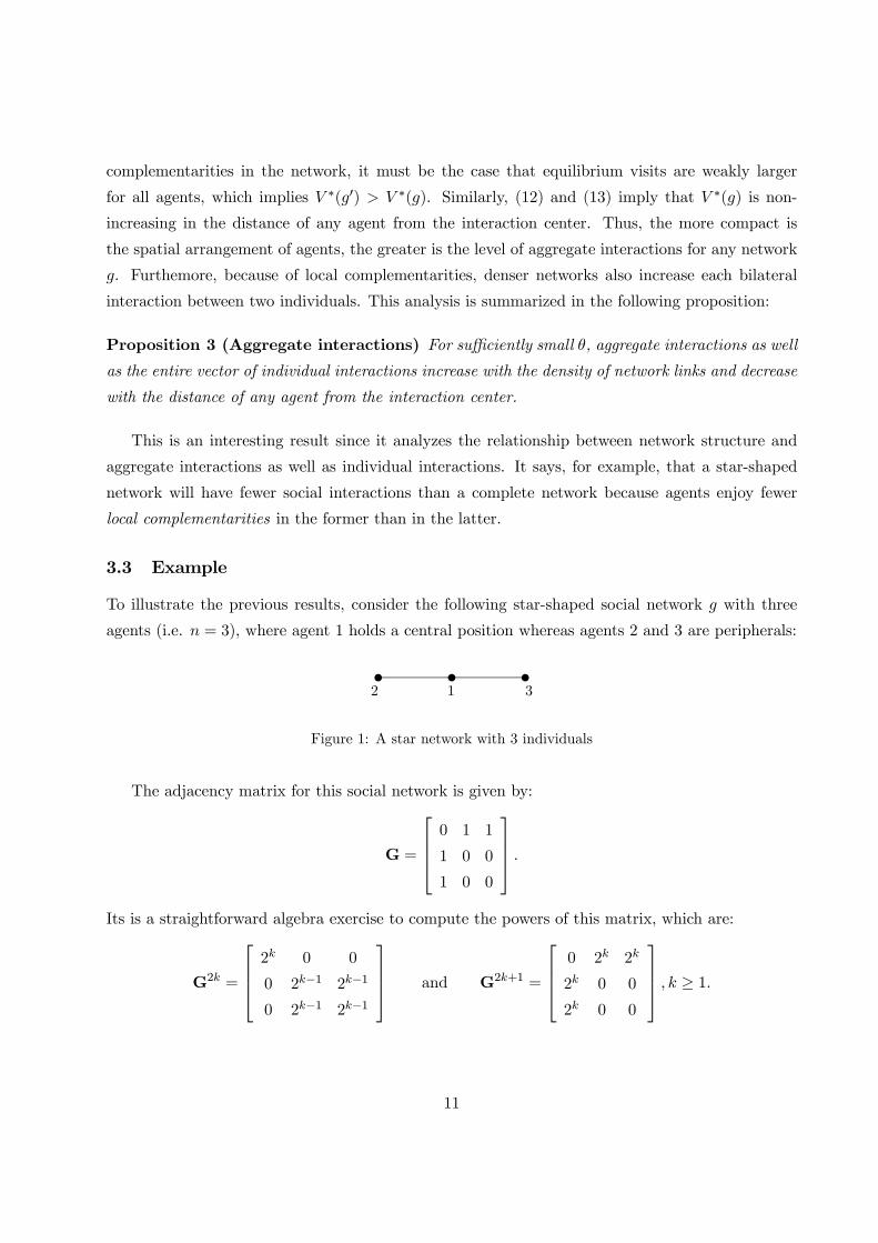
To illustrate the previous results, consider the following star-shaped social network with three
agents (i.e. = 3), where agent 1 holds a central position whereas agents 2 and 3 are peripherals:
t t t2 1 3
Figure 1: A star network with 3 individuals
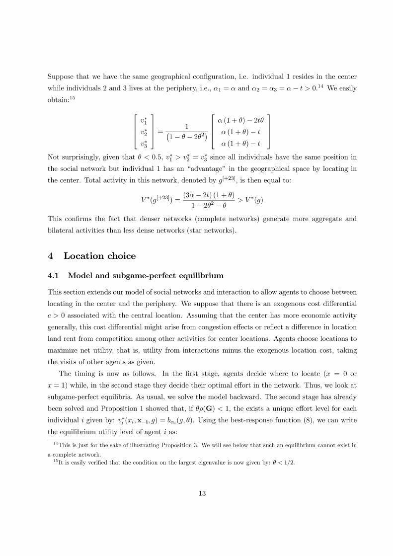
The adjacency matrix for this social network is given by:
G =
⎡⎢⎢⎣0 1 1
1 0 0
1 0 0
⎤⎥⎥⎦ Its is a straightforward algebra exercise to compute the powers of this matrix, which are:
G2 =
⎡⎢⎢⎣2 0 0
0 2−1 2−1
0 2−1 2−1
⎤⎥⎥⎦ and G2+1 =
⎡⎢⎢⎣0 2 2
2 0 0
2 0 0
⎤⎥⎥⎦ ≥ 1
11

For instance, we deduce from G3 that there are exactly two walks of length three between agents 1
and 2, namely, 12→ 21→ 12 and 12→ 23→ 32. Obviously, there is no walk of this length (and,
in general, of odd length) from any agent to herself. It is easily verified that:
M = [I− G]−1 =1
1− 22
⎡⎢⎢⎣1
1− 2 2
2 1− 2
⎤⎥⎥⎦We can now compute the agents’ centrality measures using (11). We obtain:12⎡⎢⎢⎣
∗1∗2∗3
⎤⎥⎥⎦ =⎡⎢⎢⎣
1 ( )
2 ( )
3 ( )
⎤⎥⎥⎦ = 1
1− 22
⎡⎢⎢⎣1 + (2 + 3)
1 +¡1− 2
¢2 + 23
1 + 22 +¡1− 2
¢3
⎤⎥⎥⎦Suppose now that, for exogenous reasons, individual 1 resides in the center, i.e., 1 = 0 while
individuals 2 and 3 live at the periphery, i.e., 2 = 3 = 1. This implies that 1 = and
2 = 3 = − 0. Thus, we now have:⎡⎢⎢⎣∗1∗2∗3
⎤⎥⎥⎦ = 1
1− 22
⎡⎢⎢⎣+ 2 (− )
(1 + )−
(1 + )−
⎤⎥⎥⎦ (15)
It is easily verified that:13
∗1 ∗2 = ∗3
In that case, the effort exerted by agent 1, the most central player, is the highest one. As a result,
agents located closer to the center have higher centrality ( ) and thus higher effort (i.e. they
visit more often the center to interact with other people). Note that, in equilibrium, each agent ’s
effort is affected by the location of all other agents in the network but distant neighbors have less
impact due to the decay factor in the Katz-Bonacich centrality.
The equilibrium aggregate level of interactions in a network is then given by:
∗() ==X=1
∗ =(3 + 4)− 2 (1 + ) ¡
1− 22¢Let us now illustrate Proposition 3. Consider the network described in Figure 1 and add one link
between individuals 2 and 3 so that we switch from a star-shaped network to a complete one.
12Note that this centrality measures are only well-defined when 1√2 or 2 12 (condition on the largest
eigenvalue).13Observe that this inequality is true because we have assumed that 1
√2 (this guarantees that the Katz-
Bonacich centrality is well-defined) and .
12
Suppose that we have the same geographical configuration, i.e. individual 1 resides in the center
while individuals 2 and 3 lives at the periphery, i.e., 1 = and 2 = 3 = − 0.14 We easily
obtain:15 ⎡⎢⎢⎣∗1∗2∗3
⎤⎥⎥⎦ = 1¡1− − 22¢
⎡⎢⎢⎣ (1 + )− 2 (1 + )−
(1 + )−
⎤⎥⎥⎦Not surprisingly, given that 05, ∗1 ∗2 = ∗3 since all individuals have the same position in
the social network but individual 1 has an “advantage” in the geographical space by locating in
the center. Total activity in this network, denoted by [+23], is then equal to:
∗([+23]) =(3− 2) (1 + )
1− 22 − ∗()
This confirms the fact that denser networks (complete networks) generate more aggregate and
bilateral activities than less dense networks (star networks).
4 Location choice
4.1 Model and subgame-perfect equilibrium
This section extends our model of social networks and interaction to allow agents to choose between
locating in the center and the periphery. We suppose that there is an exogenous cost differential
0 associated with the central location. Assuming that the center has more economic activity
generally, this cost differential might arise from congestion effects or reflect a difference in location
land rent from competition among other activities for center locations. Agents choose locations to
maximize net utility, that is, utility from interactions minus the exogenous location cost, taking
the visits of other agents as given.
The timing is now as follows. In the first stage, agents decide where to locate ( = 0 or
= 1) while, in the second stage they decide their optimal effort in the network. Thus, we look at
subgame-perfect equilibria. As usual, we solve the model backward. The second stage has already
been solved and Proposition 1 showed that, if (G) 1, the exists a unique effort level for each
individual given by: ∗ (x−i ) = ( ). Using the best-response function (8), we can write
the equilibrium utility level of agent as:
14This is just for the sake of illustrating Proposition 3. We will see below that such an equilibrium cannot exist in
a complete network.15 It is easily verified that the condition on the largest eigenvalue is now given by: 12.
13
∗ (∗ v
∗−i) = +
1
2[∗ (x−i )]
2= +
1
2[( )]
2 (16)
where ∗ (0x−i ) and ∗ (1x−i ) are the equilibrium effort of individual if she lives in the center
and in the periphery, respectively. As a result, the equilibrium utility of each agent is equal to
her income plus half of her equilibrium effort squared. We need now to solve the first stage of
the game, i.e. the location choice. What is complicated here is that the weighted Katz-Bonacich
centralities are endogenous equilibrium objects and thus one needs to know the equilibrium location
configuration in order to build the equilibrium.
Let us now characterize the equilibrium.
Define C as the set of central agents (i.e. all individuals who live in the center) and P as the
set of peripheral agents (i.e. all individuals who live in the periphery). If individual resides in the
center ( = 0), her equilibrium utility is equal to:16
∗ (∗ (0x−i )v
∗−i) = +
1
2
⎡⎣ X∈C−{}
+∞X=0
[] +
X∈P−{}
+∞X=0
[] (− ) +
+∞X=0
[]
⎤⎦2 −
We have here decomposed the Katz-Bonacich centrality ( ) into self-loops ( =P+∞
=0 [] )
and non self-loops ( =P+∞
=0 [] ) and give different weights to these paths depending if agents
live in the center (weight ) or in the periphery (weight − ). Similarly, if individual resides in
the periphery ( = 1), her equilibrium utility is equal to:
∗ (∗ (1x−i )v
∗−i) = +
1
2
⎡⎣ X∈C−{}
+∞X=0
[] +
X∈P−{}
+∞X=0
[] (− ) +
+∞X=0
[] (− )
⎤⎦2
As a result, individual will live at = 0 if and only if ∗ (∗ (0x−i )v
∗−i) ∗ (
∗ (1x−i )v
∗−i).
Denote by
[−] ( ) ≡
X=1 6=
= X
∈C−{} +
X∈P−{}
the weighted Katz-Bonacich centrality without self-loops and
(2) ≡
−³[−] ( )−
P∈P−{}
´+
r³[−] ( )−
P∈P−{}
´2+ 2
(2− )
2−
We have the following result:
16Observe that C−{} and P−{} denotes respectively the set of all central agents but and the set of all peripheralagents but .
14
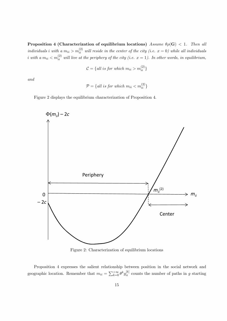
Proposition 4 (Characterization of equilibrium locations) Assume (G) 1. Then all
individuals with a (2) will reside in the center of the city (i.e. = 0) while all individuals
with a (2) will live at the periphery of the city (i.e. = 1). In other words, in equilibrium,
C = {all s for which (2) }
and
P = {all s for which (2) }
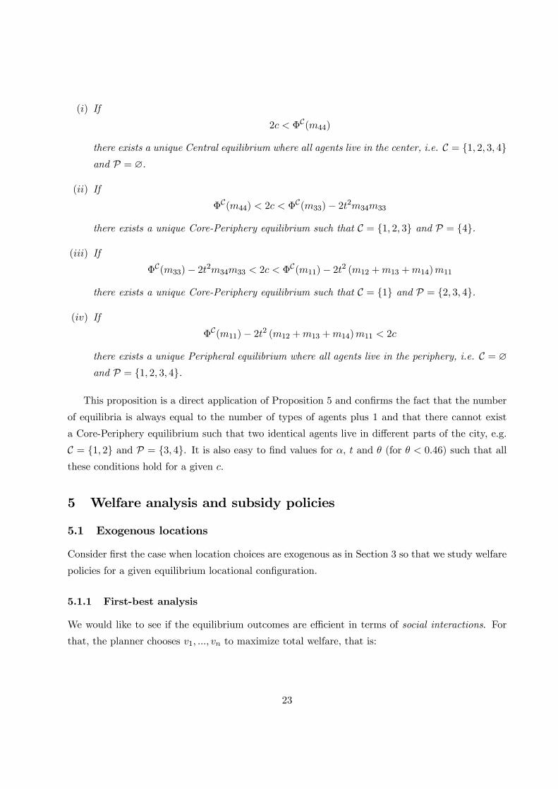
Figure 2 displays the equilibrium characterization of Proposition 4.
mii(2)
(mii) – 2c
0
Center
Periphery
mii
– 2c
Figure 2: Characterization of equilibrium locations
Proposition 4 expresses the salient relationship between position in the social network and
geographic location. Remember that =P+∞
=0 [] counts the number of paths in starting
15
from and ending at (self-loops) where paths of length are weighted by , and 6= =P+∞=0
[] counts the number of paths in starting from and ending at 6= (non self-loops)
where paths of length are weighted by . Remember also that the Katz-Bonacich centrality is:
( ) = +P
=1 6= while the weighted Katz-Bonacich centrality is given by:
( ) = + X∈C
+ (− )X∈P
where = if lives in the center and = − if lives in the periphery. As a result,
captures the centrality in the network of each individual . If participation in a social network
involves costly transportation, then agents who occupy more central positions in the social network
will have the most to gain from locating at the interaction center. In our model with two locations,
in equilibrium agents who are most central in the social network (higher ) will locate at the
interaction center, while agents who are less central in the social network (lower ) locate in the
periphery. There is, in effect, endogenous geographic separation by position in the social network.
We would now like to deal with the issues of existence and uniqueness of the subgame-perfect
equilibrium location-effort. For that, consider any network with agents. Rank agents in the
network such that we start with agent 1 who has the highest centrality in the network, i.e. 11 =
max, then we have agent 2 who has the next highest centrality, etc. until we reach agent
who has the lowest centrality in the network, i.e. = min. Define each agent by her type,
where the type of an agent is her Katz-Bonacich centrality (or her ). Since two agents can have
the same centrality, there are ≤ types in each network of agents. Denote by
Φ() ≡ (2− ) ()2 + 2
⎛⎝X
=−{}
⎞⎠ (17)
where all the s and s are defined by the cells of the matrix M = [I− G]−1. We have the
following result where “equilibrium” means “Subgame-Perfect Nash equilibrium”:
Proposition 5 (Existence and uniqueness of equilibrium locations) Assume (G) 1 and
consider any network of agents with ≤ types. In any equilibrium, two agents with the
same Katz-Bonacich centrality have to reside in the same part of the city and agents with higher
Katz-Bonacich centrality cannot reside further away from the center than agents with lower Katz-
Bonacich centrality. Moreover, the number of equilibria is equal to the number of types of agents
plus one, i.e. + 1.
If the number of types is the same as the number of agents, we can characterize the locational
(subgame-perfect) equilibria as follows:
16

() If
2 ΦC()
there exists a unique Central equilibrium where all agents live in the center, i.e. C = and
P = ∅.
() If
ΦC() 2 ΦC(−1−1)− 22−1−1−1
there exists a unique Core-Periphery equilibrium such that C = − {} and P = {}.
() If
ΦC(−1−1)− 22−1−1−1 2 ΦC(−2−2)− 22 (−2−1 +−2)−2−2
there exists a unique Core-Periphery equilibrium such that C = − { − 1 } and P =
{− 1 }.
() If
ΦC(−2−2)−22 (−2−1 +−2)−2−2 2 ΦC(−3−3)−22⎛⎝ X
∈P−3
⎞⎠−3−3
there exists a unique Core-Periphery equilibrium such that C = − { − 2 − 1 } andP = − {− 2 − 1 }.
() etc. until we arrive at agent 1 who has the highest centrality. Then,
() If
ΦC(11)− 22⎛⎝ X
∈P−{1}1
⎞⎠11 2
there exists a unique Peripheral equilibrium where all agents live in the periphery, i.e. C = ∅and P = .
If the number of types is less than the number of agents, then each step described above has to
be made by type and not by individual so that each subscript refers to types and not to individuals.
This proposition totally characterizes the (subgame-perfect Nash) equilibrium locations and
shows that there always exists a unique equilibrium within each interval. Interestingly, we could
characterize everything in terms of ΦC(), which is the “incentive function” when there is a
17
Central equilibrium, i.e. when all agents reside in the center of the city. Indeed, when, for all ,
ΦC() 2, all individuals live in the center and we have a unique Central equilibrium. Then,
when we start to move people from the center to the periphery, we need to change the weight in the
Katz-Bonacich centrality from (when living in the center) to − (when living in the periphery).This corresponds to the terms of both the right-hand side and left-hand side of each inequality
since this is what is needed to be compensated for the agents living at the periphery of the city
compared to the Central equilibrium where these agents lived in the center. Interestingly, there
cannot be multiple equilibria within the same set of parameters.
Let us now perform a comparative statics exercise of the key parameters of the model.
Proposition 6 (Spatial concentration in the center) Assume (G) 1. A decrease in the
cost of locating in the center, a decrease in marginal transport cost , or an increase in the intensity
of social interactions , will lead to more spatial concentration of agents in the center.
Proposition 6 states that a decrease in will increase the number of agents living in the cen-
ter, which leads to more spatial concentration at the interaction center. An increase in marginal
transport cost , will have a similar impact. Finally, an increase in , the intensity of social inter-
actions, will also lead to more spatial concentration in the center. Indeed, when increases, social
interactions become more valuable and, because it is costly to commute to the center from the
periphery, the spatial concentration at the interaction center increases. Therefore, this proposition
allows us to analyze how endogenous spatial location affects the contribution equilibrium efforts.
From Proposition 3, we know that aggregate interactions decrease with the distance of any agent
from the interaction center. As a result, when, for example, decreases, more agent choose to
live in the center, which, in turn, increases social interactions in the network and thus equilibrium
efforts. It is thus interesting here to see how the geographical space affects the social space.
4.2 Examples
4.2.1 Star-shaped networks: two types of agents
Let us return to the network described in Figure 1. Remember from Section 3.3, that, if 1√2,
then
M = [I− G]−1 =1
1− 22
⎡⎢⎢⎣1
1− 2 2
2 1− 2
⎤⎥⎥⎦ (18)
18
In particular, this means that,
11 =1
1− 22 and 22 = 33 =1− 2
1− 22We have the following result.
Proposition 7 (Locational equilibrium for a star-shaped network) Consider the star-shaped
network depicted in Figure 1 and assume that 1√2 = 0707.
() If
(1− ) (1 + )2 [2− (1− ) ]
2¡1− 22¢2 (19)
there exists a unique Central equilibrium where all agents live in the center, i.e. C = {1 2 3}and P = ∅.
() If
(1− ) (1 + )2 [2− (1− ) ]
2¡1− 22¢2
[2 (1 + 2)− (1 + 4)]
2¡1− 22¢2 (20)
there exists a unique Core-Periphery equilibrium where the star agent lives in the center while
the peripheral agents reside in the periphery, i.e. C = {1} and P = {2 3}.
() If
[2 (1 + 2)− (1 + 4)]
2¡1− 22¢2 (21)
there exists a unique Peripheral equilibrium where all agents live in the periphery, i.e. C = ∅and P = {1 2 3}.
This proposition shows that, for the star-shaped network, there are only three types of equilibria
(i.e. number of types plus 1). It also shows the role of and of in the location decision process.
For fixed values of , and , when we increase , we switch from a central equilibrium to a core-
periphery equilibrium and then to peripheral equilibrium. Interestingly, for fixed values of , and
, when we decrease we obtain the same types of result because an increase in means that social
interactions are more valuable and thus tend to induce people to live to the center. The effect of
an increase of is similar.
We can give some parameter values for which each condition is satisfied given that 0707.
For example, if we set = 6, = 1 and = 02, then: () if 762, there exists a unique
Central equilibrium where C = {1 2 3} and P = ∅; () if 762 886, there is a unique
Core-Periphery equilibrium where C = {1} and P = {2 3}; () if 886, there exists a unique
Peripheral equilibrium where C = ∅ and P = {1 2 3}.
19
In each case, we can calculate the equilibrium utility of each agent. For example, if we consider
the Central equilibrium, then the equilibrium utility of agent 1 is equal to:
∗1 (∗1(0 0 0 )v
∗−1) = +
2 (1 + 2)2
2¡1− 22¢2 −
while the equilibrium utilities of agents 2 and 3 are given by
∗2 (∗2(0 0 0 )v
∗−2) = ∗3 (
∗3(0 0 0 )v
∗−3) = +
2 (1 + )2
2¡1− 22¢2 −
Not surprisingly, agent 1, who is the most central agent in the network, provides a higher effort
and thus has a higher utility than the two other agents. At the other extreme, if there is a
Peripheral equilibrium, then, to calculate the equilibrium utilities of all agents, one needs to replace
2 by (− )2 and to remove the cost in the expressions above. Finally, in the Core-Periphery
equilibrium, C = {1} and P = {2 3}, we obtain:17
∗1 (∗1(0 1 1 )v
∗−1) = +
[2 (− ) + ]2
2¡1− 22¢2 −
∗2 (∗2(1 0 1 )v
∗−2) = ∗3 (
∗3(1 0 1 )v
∗−3) = +
( − + )2
2¡1− 22¢2
It is easily verified that all agents would be better off by living in the center if the cost is not too
large. This result can clearly be generalized for a star network with agents where there will be 3
types of equilibria as in Proposition 7.
4.2.2 Complete networks: One type of agent
Let us now consider a complete network and, as in the previous section, set = 3 (the generalization
to agents is straightforward). If 12, then
M = [I− G]−1 =1
1− − 22
⎡⎢⎢⎣1−
1−
1−
⎤⎥⎥⎦ (22)
We have the following result.
17 Inside the utility function, the equilibrium effort ∗ (x−i ) is written such that the first element in the
parenthesis is the location of agent while the other elements are the locations of all other agents by increasing
numbering order, starting from agent 1 if 1 6= . For example, for the star network with three agents, ∗1(0 1 1 ) is
the equilibium effort of agent 1 (the star) for the Core-Periphery equilibrium C = {1} and P = {2 3} since 1 = 0
and 2 = 3 = 1 while ∗2(1 0 1 ) is the equilibium effort of agent 2 (peripheral agent) for the same Core-Periphery
equilibrium.
20
Proposition 8 (Locational equilibrium for a complete network) Consider the complete net-
work with 3 agents and assume that 12.
() If
(1− )2 (2+ 4− )
2¡1− − 22¢2
there exists a unique Central equilibrium where all agents live in the center, i.e. C = {1 2 3}and P = ∅.
() If
(1− )2 (2+ 4− )
2¡1− − 22¢2
there exists a unique Peripheral equilibrium where all agents live in the periphery, i.e. C = ∅and P = {1 2 3}.
This proposition completely characterizes the equilibrium configuration for a complete network.
As showed in Proposition 5, there are no multiple equilibria and no core-periphery equilibrium. We
can give parameter values for which each condition is satisfied given that 05. For example,
if take exactly the same parameters as for the star network, i.e. = 6, = 1 and = 02, then:
() if 2161, there exists a unique Central equilibrium where C = {1 2 3} and P = ∅; () if
2161, there exists a unique Peripheral equilibrium where C = ∅ and P = {1 2 3}.It is straightforward to generalize this result for a complete network with agents but also for
any regular network. Using the argument of the proof, we can state that, for any regular network
(i.e. each agent has the same number of links) with agents, only two equilibria will emerge:
the Central and the Peripheral equilibrium. If is low enough, there will be a unique Central
equilibrium while, if is high enough, there will be a unique Peripheral equilibrium.
Observe that when we compare the star network and the complete network with 3 agents, we
see that there is much more clustering in the center for the latter than for the former. Indeed, if
we again consider the parameters = 6, = 1 and = 02, then when 886 2161, all the 3
agents live in the center in the complete network while they all reside in the periphery in the star
network. This is because there are much more interactions in the complete than in the star social
network because, in the former, everybody interact directly with everybody while, in the latter,
agents 1 and 2 interact directly with the star (agent 1) but only indirectly with each other. This is
in fact a general result, which is straightforward to prove, which says that the networks that favor
more interactions will have more clustering in the center than those that induce less interactions.
21
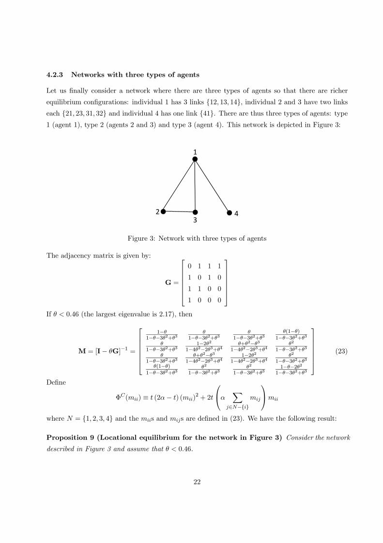
4.2.3 Networks with three types of agents
Let us finally consider a network where there are three types of agents so that there are richer
equilibrium configurations: individual 1 has 3 links {12 13 14}, individual 2 and 3 have two linkseach {21 23 31 32} and individual 4 has one link {41}. There are thus three types of agents: type1 (agent 1), type 2 (agents 2 and 3) and type 3 (agent 4). This network is depicted in Figure 3:
2
1
34
Figure 3: Network with three types of agents
The adjacency matrix is given by:
G =
⎡⎢⎢⎢⎢⎢⎣0 1 1 1
1 0 1 0
1 1 0 0
1 0 0 0
⎤⎥⎥⎥⎥⎥⎦If 046 (the largest eigenvalue is 217), then
M = [I− G]−1 =
⎡⎢⎢⎢⎢⎢⎣1−
1−−32+3
1−−32+3
1−−32+3(1−)
1−−32+3
1−−32+31−22
1−42−23+4+2−3
1−42−23+42
1−−32+3
1−−32+3+2−3
1−42−23+41−22
1−42−23+42
1−−32+3(1−)
1−−32+32
1−−32+32
1−−32+31−−22
1−−32+3
⎤⎥⎥⎥⎥⎥⎦ (23)
Define
Φ() ≡ (2− ) ()2 + 2
⎛⎝X
∈−{}
⎞⎠
where = {1 2 3 4} and the s and s are defined in (23). We have the following result:
Proposition 9 (Locational equilibrium for the network in Figure 3) Consider the network
described in Figure 3 and assume that 046.
22
() If
2 ΦC(44)
there exists a unique Central equilibrium where all agents live in the center, i.e. C = {1 2 3 4}and P = ∅.
() If
ΦC(44) 2 ΦC(33)− 223433
there exists a unique Core-Periphery equilibrium such that C = {1 2 3} and P = {4}.
() If
ΦC(33)− 223433 2 ΦC(11)− 22 (12 +13 +14)11
there exists a unique Core-Periphery equilibrium such that C = {1} and P = {2 3 4}.
() If
ΦC(11)− 22 (12 +13 +14)11 2
there exists a unique Peripheral equilibrium where all agents live in the periphery, i.e. C = ∅and P = {1 2 3 4}.
This proposition is a direct application of Proposition 5 and confirms the fact that the number
of equilibria is always equal to the number of types of agents plus 1 and that there cannot exist
a Core-Periphery equilibrium such that two identical agents live in different parts of the city, e.g.
C = {1 2} and P = {3 4}. It is also easy to find values for , and (for 046) such that all
these conditions hold for a given .
5 Welfare analysis and subsidy policies
5.1 Exogenous locations
Consider first the case when location choices are exogenous as in Section 3 so that we study welfare
policies for a given equilibrium locational configuration.
5.1.1 First-best analysis
We would like to see if the equilibrium outcomes are efficient in terms of social interactions. For
that, the planner chooses 1 to maximize total welfare, that is:
23
max1
W = max1
=X=1
(v−i)
= max1
⎧⎨⎩=X=1
∙ + − 1
22
¸+
=X=1
X=1
⎫⎬⎭First-order condition gives for each = 1 :18
− + X
+ X
= 0
which implies that (since = ):19
= + 2X
(24)
Using (8), we easily see that:
= ∗ + X
(25)
where ∗ is the Nash equilibrium number of visits given in (8). This means that there are too few
visits at the Nash equilibrium as compared to the social optimum outcome. Equilibrium interaction
effort is too low because each agent ignores the positive impact of a visit on the visit choices of
others, that is, each agent ignores the positive externality arising from complementarity in visit
choices. As a result, the market equilibrium is not efficient and the planner would like to subsidize
visits to the interaction center.
5.1.2 Subsidizing social interactions
Letting denote the optimal subsidy to per visit, comparison of (24) and (25) implies:
=
X
(26)
or in matrix form
S = Gv
18 It is easily checked that there is a unique maximum for each .19The superscript refers to the “social optimum” outcome while a star refers to the “Nash equilibrium” outcome.
24
If we add one stage before the visit game is played, the planner will announce the optimal subsidy
to each agent such that:
= +¡ +
¢ − 1
22 +
X
= + − 122 + 2
X
By doing so, the planner will restore the first best. Observe that the optimal subsidy is such that
v = (I− G)−1¡ +
¢1
= (I− 2G)−1α
where α =(1 )T, which means that
=
X=1
+∞X=0
[]
¡ +
¢=
X=1
+∞X=0
2[]
and thus
= +
1
2
£+( )
¤2= +
1
2[(2 )]
2
In particular, the optimal subsidy is given by:
=
X
=
X=1
X=1
+∞X=0
2[]
(27)
What is interesting here is that the planner will give a larger subsidy to more central agents in the
social network. Let us summarize our results by the following proposition.
Proposition 10 (Optimal level of social interactions) The Nash equilibrium outcome in terms
of social interactions is not efficient since there are too few social interactions. If the planner pro-
poses a subsidy =
P to each individual , then the first-best outcome can be restored. In
that case, it is optimal for the planner to give higher subsidies to more central agents in the social
network.
5.2 Endogenous locations
As in Section 4, assume now that agents can choose where to locate.
25
5.2.1 Effort (number of visits) subsidies
Assume that the planner cannot control location but only effort. In that case, in the second stage,
she will choose a higher level of effort given by
=
X=1
+∞X=0
2[] (28)
and then let the agents choose their location. In other words, the timing is as follows: First, agents
choose their location in the city between the center and the periphery and then the government
choose effort. The second stage is solved as above and the optimal effort is given by (28). By
plugging back this effort into the utility function, we obtain the following equilibrium optimal
utility of each agent if she lives in the center ( = 0):
(
∗ (0x−i )v
∗−i) = +
1
2
⎡⎣ X∈C−{}
+∞X=0
2[] +
X∈P−{}
+∞X=0
2[] (− ) +
+∞X=0
2[]
⎤⎦2−(29)
Similarly, if individual resides in the periphery ( = 1), her equilibrium optimal utility is equal
to:
(
∗ (1x−i )v
∗−i) = +
1
2
⎡⎣ X∈C−{}
+∞X=0
2[] +
X∈P−{}
+∞X=0
2[] (− ) +
+∞X=0
2[] (− )
⎤⎦2(30)
We can characterize the equilibrium location and it is clear that more agents will live in the center
compared to the case where they choose themselves their own effort.
Furthermore, if we investigate a constrained efficient allocation in which the planner can sub-
sidize interactions (i.e., provide a subsidy of per visit by agent ) but cannot directly control
location choices, then more agents will live in the center compared to the case without subsidies. In-
deed, since all agents devote more effort to interacting with others under the subsidy program (26),
the incentives for clustering must be stronger under that allocation than in the Subgame-Perfect
Nash equilibrium.
To see that, we can calculate the “incentive” function Φ(), which is now given by:
Φ() = 4 (2− ) ()2 + 8
⎡⎣ X∈C−{}
+ (− )X
∈P−{}
⎤⎦ (31)
= 4Φ()
where Φ() is given by (42) and is calculated when agents chose both location and effort.
Remember that this function determines the location decision of each individual . Given an
26

equilibrium configuration = CP, if Φ() 2, individual resides in the center while, if
Φ() 2, she will reside in the periphery. It is straightforward to write the equivalent of
Proposition 5 in the case when the planner chooses effort by only changing the value Φ(),
given in (17), to a new value equal to:
Φ() = 4 (2− ) ()2 + 8
⎛⎝X
=−{}
⎞⎠ = 4Φ()
Since Φ() Φ(), it is then straightforward to write the following proposition:
Proposition 11 (Equilibrium versus optimal location choices) If the planner proposes a per
visit subsidy to each individual , then, compared to the Subgame-Perfect Nash equilibrium lo-
cation choices, more agents live in the center.
To illustrate this proposition, take again the star network described in Figure 1. We easily
obtain:
Proposition 12 (Subsidizing effort in a star-shaped network) Consider the star-shaped net-
work depicted in Figure 1 and assume that 1¡2√2¢= 035 and that the planner chooses (or
subsidizes) agents’ effort.
() If
2 (1− ) (1 + )2 [2− (1− ) ]¡
1− 22¢2 (32)
there exists a unique Central equilibrium where all agents live in the center, i.e. C = {1 2 3}and P = ∅.
() If
2 (1− ) (1 + )2 [2− (1− ) ]¡1− 22¢2
2 [2 (1 + 2)− (1 + 4)]¡1− 22¢2 (33)
there exists a unique Core-Periphery equilibrium where the star agent lives in the center while
the peripheral agents reside in the periphery, i.e. C = {1} and P = {2 3}.
() If
2 [2 (1 + 2)− (1 + 4)]¡
1− 22¢2 (34)
27
Let us illustrate Proposition 11. If
(1− ) (1 + )2 [2− (1− ) ]
2¡1− 22¢2
2 (1− ) (1 + )2 [2− (1− ) ]¡1− 22¢2
then agents 1, 2 and 3 live in the center when the planner chooses effort (Proposition 12) whereas
agent 1 lives in the center while agents 2 and 3 reside in the periphery when agents choose effort
(Proposition 7). Since the sum of utilities of all agents is the sum of their Katz-Bonacich centralities
weighted by for those who reside in the center and by − for those who reside in the periphery,then total welfare is higher when the planner subsidizes effort.
Similarly, if
[2 (1 + 2)− (1 + 4)]
2¡1− 22¢2
2 [2 (1 + 2)− (1 + 4)]¡1− 22¢2
then agents 1 lives in the center while agents 2 and 3 reside in the periphery when the planner
chooses effort (Proposition 12) whereas all agents live in the periphery when agents choose effort
(Proposition 7). The total is also clearly higher when agents’ effort is subsidized. As a result, when
the planner chooses (or subsidizes) effort, then agents tend to concentrate more in the center of the
city than when she don’t.
5.2.2 Location subsidies
Let us now consider a model where the planner subsidizes location but not effort. Since there are
more interactions when agents live in the center and since interactions increase utility, then the
planner could subsidize the location cost in the center.20 In other words, she can give a per-cost
subsidy so that the cost of locating in the center would be (1− ) instead of . The timing
is now as follows. In the first stage, the planner announces the subsidy to agents locating in the
center. In the second stage, agents decide where to locate while, in the last stage, their decide their
effort level. As for the subsidy effort, this will clearly generate more clustering in the center but
the mechanism is different since, in the latter, the effect is direct while, in the former, it is indirect.
In that case, equilibrium efforts will still be determined by (11) while location decisions will be
characterized by Proposition 5 where has to be replaced by (1− ) .
In this model, it is clear that, if the planner wants to reach the first best in terms of location,
she will subsidize so that all agents will live in the center. This maximizes aggregate interactions
and thus total welfare. For example, in the case of the star network described in Figure 1, we
20 It is easily verified that a policy that subsidizes (marginal transport cost) is equivalent to a policy that subsidizes
. Therefore, we focus our analysis on a subsidy of .
28
have shown that if = 6, = 1 and = 02, then: () if 762, there exists a unique Central
equilibrium; () if 762 886, there is a unique Core-Periphery equilibrium; () if 886,
there exists a unique Peripheral equilibrium. As a result, if, for all agents, (1− ) ≤ 762, whichis equivalent to ≥ 1− (762), then the first best is reached and all workers reside in the center.For example, if = 20, then planner needs to subsidize 619 percent of the cost of living in the
center of all agents. Interestingly, this result depends on the network structure. For the complete
network with 3 agents, we have seen that, with exactly the same parameters, = 6, = 1 and
= 02, then: () if 2161, there exists a unique Central equilibrium; () if 2161, there
exists a unique Peripheral equilibrium. In that case, we need to subsidize ≥ 1−(2161) percentof for all agents to reach the first best. Thus, for the complete network, if = 20, the planner
does not need to subsidy any worker to reach the first best in efforts since 20 2161. Using this
reasoning and looking at Proposition 5, the optimal subsidy for any network with agents is given
by:
1− ΦC()
2(35)
where, from (17), we have:
Φ() ≡ (2− ) ()2 + 2
⎛⎝X
=−{}
⎞⎠ (36)
Observe that equation (35) gives the subsidy for the agent who has the lowest centrality in
the network. Indeed, if the planner gives a −subsidy of 1− £ΦC()2¤to all agents, the first
best will be reached since all individuals will be induced to reside in the center. This is clearly
a sufficient condition. The planner could also discriminate between agents and gives a different
subsidy to each agent so that the higher is the centrality of an agent in a network, the lower is the
subsidy. In that case, the subsidy to be given to each agent will be equal to:
1− ΦC()
2(37)
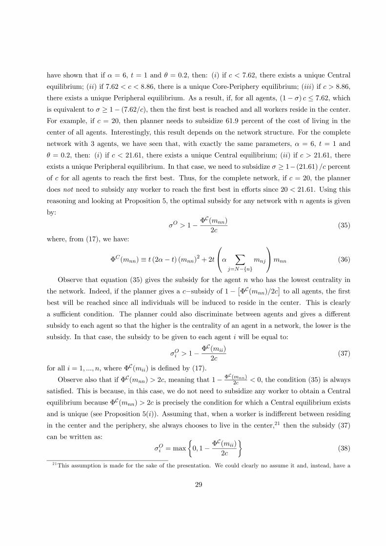
for all = 1 , where ΦC() is defined by (17).
Observe also that if ΦC() 2, meaning that 1− ΦC()2
0, the condition (35) is always
satisfied. This is because, in this case, we do not need to subsidize any worker to obtain a Central
equilibrium because ΦC() 2 is precisely the condition for which a Central equilibrium exists
and is unique (see Proposition 5()). Assuming that, when a worker is indifferent between residing
in the center and the periphery, she always chooses to live in the center,21 then the subsidy (37)
can be written as:
= max
½0 1− Φ
C()
2
¾(38)
21This assumption is made for the sake of the presentation. We could clearly no assume it and, instead, have a
29

5.2.3 Effort versus location subsidy
Let us now study both the effort and location subsidies. We have seen that if the planner only
subsidizes effort, then the optimal subsidy is given by (27), that is
=
X=1
X=1
+∞X=0
2[]
This optimal subsidy clearly depends on agents’ locations. As a result, the first best when both
locations and efforts are taken into account should be when the effort subsidy is and all agents
live in the center. The timing is now as follows: First, the planner announces the location and the
effort subsidies. Second, agents choose their location. Third, agents choose efforts.
DenoteM = (I− 2G)−1 so that the element of the th and th ofM is .22 Then, using
the same reasoning as above, the location subsidy and the effort subsidy that guarantee that the
first best (when both locations and efforts are taken into account) is achieved is determined in the
following proposition:
Proposition 13 (First best with effort and location subsidies) Assume 2(G) 1 and
consider any network of agents. If the location subsidy and the effort subsidy for each agent
are such that ⎧⎨⎩ = maxn0 1− 2ΦC(
)
o =
P=1
P=1
P+∞=0 2
[]
then all agents live in the center and provide optimal interaction efforts (number of visits) and
therefore the first best is achieved.
This proposition implies that, to reach the first best, it is optimal for the the planner to give
higher effort subsidies but lower location subsidies to more central agents in the social network.
If we consider the star network of Figure 1, it is readily verified that, if 1¡2√2¢= 035,
subsidy equal to:
= max
0 1− ΦC()
2+
where is very small.22Remember that, when the per-effort subsidy is given to each agent , she provides an optimal effort
, which
is defined by:
v= (I− 2G)−1 =M
30

then, if all agents live in the center (i.e. 1 = 2 = 3 = ), we have:
Mα = (I− 2G)−1α = ¡1− 82¢
⎛⎜⎜⎝1 + 4
1 + 2
1 + 2
⎞⎟⎟⎠so that ⎛⎜⎜⎝
1
2
3
⎞⎟⎟⎠ =¡
1− 82¢⎛⎜⎜⎝1 + 4
1 + 2
1 + 2
⎞⎟⎟⎠Since the optimal effort subsidy for each agent is given by:
=
X
or in matrix form
S = Gv
We have
1 =
¡2 + 3
¢= 2
µ1 + 2
1− 82¶
2 =
3 = 1 =
µ1 + 4
1− 82¶
Not surprisingly, the planner gives more effort subsidy to more central agents since 1
2 .
Now, let us calculate the location subsidy. The matrix M is given by
M = (I− 2G)−1= 1¡1− 82¢
⎛⎜⎜⎝1 2 2
2 1− 42 42
2 42 1− 42
⎞⎟⎟⎠As a result,
Φ(11) = (2− )
¡11
¢2+ 2
¡12 +
13
¢11
= [2 (1 + 4)− ]¡
1− 82¢2Thus, the subsidy given to agent 1 is equal to:
1 = max
(0 1− [2 (1 + 4)− ]
2¡1− 82¢2
)
31

Simarly, we have:
Φ(22) = Φ(
33) = (2− )¡22
¢2+ 2
¡21 +
23
¢22
=¡1− 42¢ (1 + 2) [2− (1− 2)]¡
1− 82¢2Thus, the subsidy 2 = 3 to give to agents 2 and 3 is:
2 = max
(0 1−
¡1− 42¢ (1 + 2) [2− (1− 2)]
2¡1− 82¢2
)
As expected, it is easily verified that 1 2 , i.e. the planner gives less location subsidy to more
central agents.
Take again = 6, = 1 and = 02, then the planner needs to give the following subsidies:
1 = 494 and
2 = 3 = 318
and
1 = max
½0 1− 2228
¾and 2 = 3 = max
½0 1− 1450
¾to reach the first best. If, for example, = 20, then the planner does not need to subsidize agent 1
but need to subsidy 275 percent of the location cost to live in the center for agents 2 and 3.
Consider now the complete network with the three agents residing in the center. It is easily
verified that, if 025,
1 =
2 = 3 = =
2 (1 + 2)¡1− 2 − 82¢
1 = 2 = 3 = = max
(0 1− (1− 2) [2 (1 + 2)− (1− 2)]
2¡1− 2 − 82¢2
)If we take the same parameter values, = 6, = 1 and = 02, then = 12 and
= max
½0 1− 1736
¾If we compare the two networks, it easily verified that the planner needs to subsidize much more
the social effort of all agents in the complete network (there are more network externalities in the
complete network compared to the star network) while, for a given and for location subsidies, she
needs to subsidize less agent 1 but more agents 2 and 3 in the star network. In terms of network
design, this means that the planner would not always like to choose the complete network, even
though it is the network that generates most interactions among all possible networks. The optimal
network will clearly depend on parameters values and will be, in general, difficult to determine.
32
6 Spatial mismatch and policy issues
There is an important literature in urban economics showing that, in the United States, distance
to jobs is harmful to workers, in particular, black workers. This is known as the “spatial mismatch
hypothesis”. Indeed, first formulated by Kain (1968), the spatial mismatch hypothesis states that,
residing in urban segregated areas distant from and poorly connected to major centres of employ-
ment growth, black workers face strong geographic barriers to finding and keeping well-paid jobs.
In the US context, where jobs have been decentralized and blacks have stayed in the central parts
of cities, the main conclusion of the spatial mismatch hypothesis is that distance to jobs is the
main cause of their high unemployment rates. Since Kain’s study, hundreds of others have been
conducted trying to test the spatial mismatch hypothesis (see, in particular, the literature sur-
veys by Ihlanfeldt and Sjoquist, 1998; Ihlanfeldt, 2006; Gobillon et al., 2007; Zenou, 2008). The
usual approach is to relate a measure of labor-market outcomes, typically employment or earn-
ings, to another measure of job access, typically some index that captures the distance between
residences and centres of employment. The general conclusions are: () poor job access indeed
worsens labor-market outcomes, () black and Hispanic workers have worse access to jobs than
white workers, and () racial differences in job access can explain between one-third and one-half
of racial differences in employment. Interpret the model in terms of black and white workers.
Our model can shed new light on the “spatial mismatch hypothesis” debate by putting forward
the importance of, not only the geographical space (distance to jobs), but also the social space in
explaining the adverse labor-market outcomes of black workers.
Let us interpret our model in the following way. There are two locations, a center, where all
jobs are located and all interactions take place, and a periphery.23 Here an interaction between
two individuals means that they exchange job information with each other and thus each visit to
the center implies a job-information exchange with someone. As above, is the number of visits
that individual makes to the center in order to obtain information about jobs and each visit
results in one interaction. We do not explicitly model the labor market. We just assume that the
higher is the number and quality24 of interactions, the higher is the quality of job information and
the higher is the probability of being employed.25 In other words, each time a person goes to the
center, she interacts with someone and obtains a piece of job information, which is proportional to
23Observe that, in the context of real-world cities, the center does not necessarily mean the physical center of the
city but the place where jobs and interactions take place.24 In equilibrium, more central workers provide higher quality job information because they interact more with
others than less central workers.25This is the basic idea behind most network models of the labor market such as Calvó-Armengol (2004), Calvó-
Armengol and Jackson (2004), Calvó-Armengol and Zenou (2005) and Ioannides and Soetevent (2006).
33
the network centrality of the individual she meets. This leads to a positive relationship between
, the individual number of visits to the center, and , the employment rate of each individual
. Underlying this idea is some form of information imperfection in which networks serve at least
partially to mitigate these imperfections.26
There are two types of workers: black and white individuals. The only difference between
black and white workers is their position in the network. We assume that whites have a more
central position (in terms of Katz-Bonacich centrality) in the network than blacks. This captures
the idea of the “old boy network” where whites grew up together, went through school together,
socialized together during adolescence and early adulthood, and entered the labor force together
(Wial, 1991).27 There is strong evidence that indicates that labor-market networks are partly race
based, operating more strongly within than across races (Ioannides and Loury, 2004; Hellerstein
et al., 2011) and that the social network of black workers is of lower quality than that of whites
(Frijters et. al., 2005; Fernandez and Fernandez-Mateo, 2006; Battu et al., 2011).
To understand the interpretation of the current model, consider the network with three types
of agents displayed in Figure 3 and assume that individuals 1, 2 and 3 are white workers while
individual 4 is a black worker. We have shown in Section 4.2.3 that if
ΦC(44) 2 ΦC(33)− 223433
there exists a unique Core-Periphery equilibrium such that C = {1 2 3} and P = {4}. In thelabor-market interpretation of this model, white workers will experience a higher employment rate
than the black worker because they will have much more information about jobs. In other words,
the white workers, especially individual 1, will interact much more with other workers than the
black worker because the latter will visit less often the center and will gather little information
about jobs. In this model, it is assumed that any worker can give information about job but the
quality of information she gives is proportional her , the number of visits she makes to the center
or equivalently the number of interactions she has with others. As stated above, the employment
probability of each worker is then proportional to the information she has gathered in equilibrium.
In this interpretation of the model, we have shown that black workers make less visits to the
center (Proposition 1) and thus interact less with other workers in the network, in particular, with
very central agents than whites. We have also shown that black workers will choose to locate
further away from jobs than white workers (Proposition 5) precisely because they interact less with
26See Ioannides and Loury (2004) and Topa (2011) for a review of the evidence on labor market networks.27Calvó-Armengol and Jackson (2004) show that an equilibrium with a clustering of workers with the same status
is likely to emerge since, in the long run (i.e. steady state), employed workers tend to be friends with employed
workers. In this model, if because of some initial condition some black workers are unemployed, then in steady-state
they will still be unemployed because both their strong and weak ties will also be unemployed.
34
central workers. At the extreme, we could have an equilibrium where all white workers live in the
center while all black workers reside in the periphery (as in the example above where C = {1 2 3}and P = {4}). This would imply that whites will interact with others much more than blacks andthat whites will interact more with whites (since they will have a very high effort in equilibrium)
than with blacks. Blacks will just interact less and thus will have much less information about
jobs. This will clearly have dramatic consequences in the labor market and will explain why black
workers experience a lower employment rate than white workers. Indeed, less central agents in the
network (i.e. black workers who do not have an old-boy network) will reside further away from jobs
(i.e. in the periphery) than more central agents (whites) and thus will have adverse labor-market
outcomes. In other words, the lack of good job contacts would be here a structural consequence of
the social isolation of inner-city neighborhoods.28 Importantly, the causality goes from the social
space to the geographical space so that it is the social mismatch (i.e. their “bad” location in the
social network) of black workers that leads to their spatial mismatch (i.e. their “bad” location in
the geographical space). Observe that the network structure is crucial in our model. For example,
in a complete network (or any regular network), there will be no effect since black and white workers
will be totally identical. As a result, the more the network is heterogenous and asymmetric, the
worse are the labor-market outcomes for black workers.29
Interestingly, Zenou (2013) has developed a model where the causality goes the other way
around. In his model, which is quite different since the labor market is explicitly model but the
social network is just captured by dyads, it is the spatial mismatch of black workers (due to housing
discrimination) that leads to their social mismatch (i.e. less interaction with white weak ties) and
thus their adverse labor-market outcomes.
For the policy implications of each model, it is crucial to know the sense of causality. If, as in
Zenou (2013), it is the geographical space that causes the social mismatch of black workers, then
the policies should focus on workers’ geographical location, as in the spatial mismatch literature. In
that case, neighborhood regeneration policies would be the right tool to use. Such policies have been
implemented in the US and in Europe through the enterprise zone programs and the empowerment
zone programs (e.g. Papke, 1994; Bondonio and Greenbaum, 2007; Ham et al., 2011; Busso et al.,
28Observe that we interpret here the “periphery” location of our model as an “inner-city neighborhood” because
what characterizes the latter is not its location in the city but the fact that it is disconnected (or badly connected)
from job centers.29There is evidence showing that, though networks are a popular method of finding a job for the ethnic minorities,
they are not necessarily the most effective in terms of gaining employment (Frijters et al., 2005; Fernandez and
Fernandez-Mateo, 2006; Battu et al., 2011). Our labor-network model could explain this fact since minority workers
tend to have less central positions in the network and tend to interact less with white workers (who have more central
positions) because they live further away from interaction centers.
35
2012). The enterprise zone policy consists in designating a specific urban (or rural) area, which
is depressed, and targeting it for economic development through government-provided subsidies to
labor and capital. The aim of the empowerment zone program is to revitalize distressed urban
communities and it represents a nexus between social welfare policy and economic development
efforts. By implementing these types of policies, one brings jobs to people and thus facilitates the
flows of job information in depressed neighborhoods. Another way of reducing the spatial mismatch
of black workers would be to implement a transportation policy that subsidizes workers’ commuting
costs (Pugh, 1998). In the United States, a number of states and counties have used welfare block
grants and other federal funds to support urban transportation services for welfare recipients. For
example, programs helping job takers (especially African Americans) obtain a used car — a secured
loan for purchase, a leasing scheme, a revolving credit arrangement — may offer real promise and
help low-skill workers obtain a job by commuting to the center where jobs are located.
If, on the contrary, as in the current model, it is the social space that causes the spatial
mismatch of black workers, then the policies should focus on workers’ social isolation. Policies
that promote social integration and thus increase the interracial interactions between black and
white workers would also have positive effects on the labor-market outcomes of minority workers.
Such policies, like the Moving to Opportunity (MTO) programs (Katz et al., 2001; Rosenbaum and
Harris, 2001; Kling et al., 2005), have been implemented in the United States. By giving housing
assistance to low-income families, the MTO programs help them relocate to better and richer
neighborhoods. For example, Rosenbaum and Harris (2001) show that: “After moving to their
new neighborhoods, the Section 8 respondents (treated group) were far more likely to be actively
participating in the labor force (i.e. working or looking for a job), while for MTO respondents, a
statistically significant increase is evident only for employment per se.” Another way of reducing
the unemployment rate of minorities in the context of our model is to observe that institutional
connections can be engineered to create connections between job seekers and employers in ways
that parallel social network processes. For example, scholars like Granovetter (1979) and Wilson
(1996) have called for poverty reduction programs to “create connections” between employers and
poor and disadvantaged job seekers.
This is ultimately an empirical question of causality − whether people that are central in thenetwork move to the city, or do people that are less connected move to the city and then become
more central. Such an empirical test is crucial but one would need either a natural experiment
with an exogenous shock or convincing instruments to break the sense of causality. In the labor-
market interpretation, the key issues is whether black workers first choose to live in geographically
isolated neighborhoods (or are forced to live there because of housing discrimination) and then
become isolated in the social space because of the lack of contacts with white workers, or do black
36
workers mainly prefer to interact with other black individuals and as a consequence locate in areas
where few whites live, which are isolated from jobs. In any case, we believe that the social and
the geographical space are intimately related and policies should take into account both of them if
they want to be successful.
Finally, using the current model, one could also examine the role of the network structure of the
labor-market outcomes of black workers. We have seen that labor-market networks are partly race
based, operating more strongly within than across races (Ioannides and Loury, 2004; Hellerstein et
al., 2011) and that more regular social networks lead to less geographical segregation and better
labor-market outcomes for black workers. Are social networks regular or very asymmetric? How
do black and white workers interact in a network? Our welfare analysis developed in Section 5 will
also be useful. In Section 5.2.3, we have seen that there is a trade off between subsidizing effort
(or the number of visits to the center) and location (or the transportation cost ). In terms of the
policies discussed above, subsidizing effort in the social space or location in the geographical space
will be equivalent to the MTO programs in the sense that it favors interactions between people by
locating them close to each other.
7 Concluding remarks
This paper provides what we believe to be the first analysis of the interaction between position in
a social network and position in a geographic space, or between social and physical distance. We
have developed a model in which agents who are more central in a social network, or are located
closer to an interaction center, choose higher levels of interaction effort in equilibrium. As a result,
the level of interactivity in the economy as a whole rises with density of links in the social network
and with the degree to which agents are clustered in physical space. When agents can choose
geographic locations, there is a tendency for those who are more central in the social network to
locate closer to the interaction center.
There are many potential extensions and applications of the work described here. First, we have
assumed that all interactions occur at a single, exogenous interaction center. In reality, interactions
in cities occur at many sites, and whether a site becomes a focal point for interactions is of course
endogenous. As in all models of complementarity, there is an interesting coordination problem in
the endogenous determination of the location of an interaction center in this model.
Second, we have developed a model where efforts are strategic complements, i.e. 0. It would
be interesting to assume instead that efforts are strategic substitutes, i.e. 0 (as in Bramoullé
and Kranton, 2007), or, following Bramoullé et al. (2012), extend parts of the analysis to allow for
a larger set of parameters (i.e. the entire range of ). The analysis would certainly be much more
37
complicated since some agents will free ride on others and provide zero effort. The interpretation
of the results will also be different.
Finally, in the present paper, we focus on fixed networks. Where we live crucially determines
whom we interact with and indeed a main attraction of big cities is that they provide more oppor-
tunities to meet new people. So network endogeneity could be an important feature of the interplay
between social networks and geographic locations. As a result, it would be interesting to extend
the model to have an endogenous network formation. We believe that it will be very difficult to
obtain clear-cut results since it is well-known that there are combinatorial (coordination) equilib-
rium multiplicity in standard network-formation models (see e.g. Jackson and Wolinsky, 1996).
Here agents also choose effort and location so coordination problems will even be more severe. One
possible way out could be to use the Cabrales et al. (2011) approach where network formation is
not the result of an earmarked socialization process so that there is a generic socialization effort.
Another way out would be to use the dynamic model of König et al. (2012) where, at each period
of time, one agent is chosen at random to form a link with others. It is clear that endogeneizing
the structure of the network would be a very difficult task given that agents also choose effort and
location. We leave this at a future research area.
References
[1] Akerlof, G. (1997), “Social distance and social decisions,” Econometrica 65, 1005-1027.
[2] Argazi, M. and V. Henderson (2008), “Networking off Madison avenue,” Review of Economic
Studies 75, 1011-1038.
[3] Ballester, C., Calvó-Armengol, A. and Y. Zenou (2006), “Who’s who in networks. Wanted:
The key player,” Econometrica 74, 1403-1417.
[4] Battu, H., Seaman, P. and Y. Zenou (2011), “Job contact networks and the ethnic minorities,”
Labour Economics 18, 48-56.
[5] Bayer, P., Ross, S.L. and G. Topa (2008), “Place of work and place of residence: Informal
hiring networks and labor market outcomes,” Journal of Political Economy 116, 1150-1196.
[6] Beckmann, M.J. (1976), “Spatial equilibrium in the dispersed city,” In: G.J. Papageorgiou
(Ed.), Mathematical Land Use Theory, Lexington, MA: Lexington Books, pp. 117-125.
[7] Benabou, R. (1993), “Workings of a city: Location, education, and production,” Quarterly
Journal of Economics 108, 619-652.
38
[8] Benabou, R. (1996), “Equity and efficiency in human capital investment: The local connec-
tion,” Review of Economic Studies 63, 237-264.
[9] Bonacich, P. (1987), “Power and centrality: A family of measures,” American Journal of
Sociology 92, 1170-1182.
[10] Bondonio, D. and R.T. Greenbaum (2007), “Do local tax incentives affect economic growth?
What mean impact miss in the analysis of enterprise zone policies,” Regional Science and
Urban Economics 37, 121-136.
[11] Bramoullé, Y. and R. Kranton (2007), “Public goods in networks,” Journal of Economic Theory
135, 478-494.
[12] Bramoullé, Y., Kranton, R. and M. D’Amours (2012), “Strategic Interaction and Networks,”
Unpublished manuscript, Duke Univerity.
[13] Brueckner, J.K. (2006), “Friendship networks,” Journal of Regional Science 46, 847-865.
[14] Brueckner, J.K. and A.G. Largey (2008), “Social interactions and urban sprawl,” Journal of
Urban Economics 64, 18-34.
[15] Brueckner, J.K., Thisse, J-F. and Y. Zenou (2002), “Local labor markets, job matching and
urban location,” International Economic Review 43, 155-171.
[16] Busso, M., Gregory, J. and P. Kline (2012), “Assessing the incidence and efficiency of a promi-
nent place based policy,” American Economic Review, forthcoming.
[17] Cabrales, A., Calvó-Armengol, A. and Y. Zenou (2011), “Social interactions and spillovers,”
Games and Economic Behavior 72, 339-360.
[18] Calvó-Armengol, A. (2004), “Job contact networks”, Journal of Economic Theory 115, 191-
206.
[19] Calvó-Armengol, A. and M.O. Jackson (2004), “The effects of social networks on employment
and inequality,” American Economic Review 94, 426-454.
[20] Calvó-Armengol, A., Patacchini, E., and Y. Zenou (2009), “Peer effects and social networks
in education,” Review of Economic Studies 76, 1239-1267.
[21] Calvó-Armengol, A. and Y. Zenou (2005) “Job matching, social network and word-of-mouth
communication”, Journal of Urban Economics 57, 500-522.
39
[22] De Bartolome, C. (1990), “Equilibrium and inefficiency in a community model with peer group
effects,” Journal of Political Economy 98, 110-33.
[23] Durlauf, S.N. (1996), “A theory of persistent income inequality,” Journal of Economic Growth
1, 75-93.
[24] Epple, D. and R.E. Romano (1998), “Competition between private and public schools, vouch-
ers, and peer-group effects,” American Economic Review 88, 33-62.
[25] Fernandez, R.M. and I. Fernandez-Mateo (2006), “Networks, race, and hiring,” American
Sociological Review 71, 42-71.
[26] Frijters, P., Shields, M.A. and S. Wheatley Price (2005), “Job search methods and their success:
A comparison of immigrants and natives in the UK,” Economic Journal 115, F359-F376.
[27] Fujita, M. and J.-F. Thisse (2002), Economics of Agglomeration. Cities, Industrial Location,
and Regional Growth, Cambridge: Cambridge University Press.
[28] Fujita, M. and H. Ogawa (1980), “Equilibrium land use patterns in a nonmonocentric city,”
Journal of Regional Science 20, 455-475.
[29] Gaspar, J. and E.L. Glaeser (1997), “Information technology and the future of cities,” Journal
of Urban Economics 43, 136-156.
[30] Gobillon, L., Selod, H. and Y. Zenou (2007), “The mechanisms of spatial mismatch,” Urban
Studies 44, 2401-2427.
[31] Ghiglino, C. and A. Nocco (2012), “When Veblen meets Krugman,” Unpublished manuscript,
University of Essex.
[32] Glaeser, E.L. (1999), “Learning in cities,” Journal of Urban Economics 46, 254-277.
[33] Glaeser, E.L. Sacerdote, B., and J. Scheinkman (1996), “Crime and social interactions,” Quar-
terly Journal of Economics 111, 508-548.
[34] Glaeser, E.L., Sacerdote, Bruce I. and J.A. Scheinkman (2003), “The social multiplier,” Journal
of the European Economic Association 1, 345-353.
[35] Glaeser, E.L. and J.A. Scheinkman (2001), “Measuring social interactions,” In: S. Durlauf and
P. Young (Eds.), Social Dynamics, Cambridge, MA: MIT Press, pp. 83-131.
40
[36] Goyal, S. (2007), Connections: An Introduction to the Economics of Networks, Princeton:
Princeton University Press.
[37] Granovetter, M.S. (1979), “Placement as brokerage: Information problems in the labor market
for rehabilitated workers,” In: D. Vandergoot and J.D. Worrall (Eds.), Placement in Reha-
bilitation: A Career Development Perspective, Baltimore, MD: University Park Press, pp.
83-101.
[38] Grauwin, S., Goffette-Nagot, F. and P. Jensen (2012), “Dynamic models of residential segre-
gation: An analytical solution,” Journal of Public Economics 96, 124-141.
[39] Ham, J.C., Swenson, C., Imrohoroglu, A. and H. Song (2011), “Government programs can
improve local labor markets: Evidence from State Enterprise Zones, Federal Empowerment
Zones and Federal Enterprise Community,” Journal of Public Economics 95, 779-797.
[40] Hellerstein, J.K., McInerney, M. and D. Neumark (2011), “Neighbors and coworkers: The
importance of residential labor market networks,” Journal of Labor Economics 29, 659-695.
[41] Helsley, R.W. and W.C. Strange (2004), “Knowledge barter in cities,” Journal of Urban Eco-
nomics 56, 327-345.
[42] Helsley, R.W. and W.C. Strange (2007), “Urban interactions and spatial structure,” Journal
of Economic Geography 7, 119-138.
[43] Ihlanfeldt, K.R. (2006), “A primer on spatial mismatch within urban labor markets,” In:
R. Arnott and D. McMillen (Eds.), A Companion to Urban Economics, Boston: Blackwell
Publishing, pp. 404-417.
[44] Ihlanfeldt, K. R. and D. Sjoquist (1998), “The spatial mismatch hypothesis: A review of recent
studies and their implications for welfare reform,” Housing Policy Debate 9, 849-892.
[45] Ioannides, Y.M. (2012), From Neighborhoods to Nations: The Economics of Social Interac-
tions, Princeton: Princeton University Press.
[46] Ioannides, Y.M. and D.L. Loury (2004), “Job information networks, neighborhood effects, and
inequality,” Journal of Economic Literature 42, 1056-1093.
[47] Ioannides, Y.M. and A.R. Soetevent (2006), “Wages and employment in a random social net-
work with arbitrary degree distribution,” American Economic Review Papers and Proceedings
96, 270-274.
41
[48] Jackson, M.O. (2008), Social and Economic Networks, Princeton: Princeton University Press.
[49] Jackson, M.O and A. Wolinsky (1996), “A strategic model of social and economic networks,”
Journal of Economic Theory 71, 44-74.
[50] Jackson, M.O. and Y. Zenou (2013), “Games on networks,“ In: P. Young and S. Zamir (Eds.),
Handbook of Game Theory, Vol. 4, Amsterdam: Elsevier, forthcoming.
[51] Jacobs, J. (1969), The Economy of Cities, New York: Vintage.
[52] Jaffe, A.B., Trajtenberg, M. and R. Henderson (1993), “Geographic localization of knowledge
spillovers as evidenced by patent citations,” Quarterly Journal of Economics 108, 577-598.
[53] Johnson, C. and R.P. Gilles (2000), “Spatial social networks,” Review of Economic Design 5,
273-299.
[54] Kain, J. (1968), “Housing segregation, negro employment, and metropolitan decentralization,”
Quarterly Journal of Economics 82, 175-197.
[55] Katz, L. (1953), “A new status index derived from sociometric analysis,” Psychometrika 18,
39-43.
[56] Katz, L.F., Kling, J.R. and J.B. Liebman (2001), “Moving to opportunity in Boston: Early
results of a randomized mobility experiment,” Quarterly Journal of Economics 116, 607-654.
[57] Kling, J.R., Ludwig, J. and L.F. Katz (2005), “Neighborhood effects on crime for female and
male youth: Evidence from a randomized housing voucher experiment,” Quarterly Journal of
Economics 120, 87-130.
[58] König, M., Tessone, C. and Y. Zenou (2012), “Nestedness in networks: A theoretical model
and some applications”, Unpublished manuscript, Stockholm University.
[59] Lucas, R.E. (1988), “On the mechanics of economic development,” Journal of Monetary Eco-
nomics 22, 3-42.
[60] Lucas, R.E. and E. Rossi-Hansberg (2002), “On the internal structure of cities,” Econometrica
70, 1445-1476.
[61] Marshall, A. (1890), Principles of Economics. London: Macmillan.
[62] Monderer, D. and L.S. Shapley (1996), “Potential games,” Games and Economic Behavior 14,
124-143.
42

[63] Moretti, E. (2004), “Workers’ education, spillovers, and productivity: Evidence from plant-
level production functions,” American Economic Review 94, 656-690.
[64] Mossay P. and P.M. Picard (2011), “On spatial equilibria in a social interaction Model, Journal
of Economic Theory 146, 2455-2477.
[65] Mossay P. and P.M. Picard (2012), “Spatial segregation and urban structure,” Unpublished
manuscript, University of Luxemburg.
[66] Papke, L. (1994), “Tax policy and urban development: evidence from the Indiana enterprise
zone program,” Journal of Public Economics 54, 37-49.
[67] Patacchini, E. and Y. Zenou (2012), “Ethnic networks and employment outcomes,” Regional
Science and Urban Economics 42, 938-949.
[68] Picard, P.M. and T. Tabuchi (2010), “Self-organized agglomerations and transport costs,”
Economic Theory 42, 565-589.
[69] Pugh, M. (1998), ”Barriers to work: the spatial divide between jobs and welfare recipients in
metropolitan areas”, Washington, DC: The Brookings Institution.
[70] Putnam, R.D. (1993), Bowling Alone: The Collapse and Revival of American Community,
New York: Simon and Schuster.
[71] Romer, P.M. (1986), “Increasing returns and long-run growth,” Journal of Political Economy
94, 1002-1037.
[72] Romer, P.M. (1990), “Endogenous technological change,” Journal of Political Economy 98,
S71-S102.
[73] Rosenbaum, E. and L.E. Harris (2001), “Residential mobility and opportunities: Early impacts
of the Moving to Opportunity demonstration program in Chicago,” Housing Policy Debate 12,
321-346.
[74] Rosenthal, S.S. and W.C. Strange (2003), “Geography, industrial organization, and agglomer-
ation,” Review of Economics and Statistics 85, 377-393.
[75] Rosenthal, S.S. and W. C. Strange (2008), “The attenuation of human capital externalities,”
Journal of Urban Economics 64, 373-389.
[76] Schelling, T.C. (1971), “Dynamic models of segregation,” Journal of Mathematical Sociology
1, 143-186.
43
[77] Topa, G. (2001), “Social interactions, local spillovers and unemployment,” Review of Economic
Studies 68, 261-295.
[78] Topa, G. (2011), “Labor markets and referrals,” In: J. Benhabib, A. Bisin and M.O. Jackson
(Eds.), Handbook of Social Economics, Vol. 1B, Amsterdam: Elsevier Science, pp. 1193-1221.
[79] Verdier, T. and Y. Zenou (2004), “Racial beliefs, location and the causes of crime,” Interna-
tional Economic Review 45, 727-756.
[80] Wasserman, S. and K. Faust (1994), Social Network Analysis. Methods and Applications,
Cambridge: Cambridge University Press.
[81] Wial, H. (1991), “Getting a good job: Mobility in a segmented labor market,” Industrial
Relations 30, 396-416.
[82] Wilson, W.J. (1996), When Work Disappears: The World of the New Urban Poor, New York:
Knopf.
[83] Zenou, Y. (2008), “The spatial mismatch hypothesis,” In: L. Blume and S. Durlauf (Eds.),
The New Palgrave, A Dictionary of Economics, Second Edition, London: MacMillan Press.
[84] Zenou, Y. (2009), Urban Labor Economics, Cambridge: Cambridge University Press.
[85] Zenou, Y. (2013), “Spatial versus social mismatch,” Journal of Urban Economics 74, 113-132.
[86] Zhang, J. (2004), “Residential segregation in an all-integrationist world,” Journal of Economic
Behavior and Organization 54, 533-550.
44
Appendix
Proof of Proposition 2. Observe that this game is a potential game (as defined by Monderer
and Shapley, 1996)30 with potential function:31
(v ) =
X=1
(vg)−
2
X=1
X=1
=
X=1
− 12
X=1
2 +
2
X=1
X=1
or in matrix form:
(v ) = v>1−12v>v + v>
2Gv
= v>1−12v> (I−G)v
It is well-known (see e.g., Monderer and Shapley, 1996) that solutions of the programmaxv (v )
are a subset of the set of Nash equilibria. This program has a unique interior solution if the potential
function (v ) is strictly concave on the relevant domain. The Hessian matrix of (v ) is
easily computed to be − (I−G). The matrix I−G is positive definite if for all non-zero v
v> (I−G)v 0⇔
µv>Gvv>v
¶−1
By the Rayleigh-Ritz theorem, we have (G) = supv 6=0³v>Gvv>v
´. Thus a necessary and sufficient
condition for having a strict concave potential is that (G) 1, as stated in the Proposition.
Proof of Proposition 4. Define C as the set of all central agents (i.e. all individuals wholive in the center) and P as the set of all peripheral agents (i.e. all individuals who live in the
periphery). Observe that C − {} and P − {} denotes respectively the set of all central agents but and the set of all peripheral agents but . The condition for which, a given prefers to live in the
30A game is a potential game if there is a function : → R such that, for each ∈ , for each − ∈ −, and
for each ∈ ,
( −)− ( −) = ( −)− ( −)
31Here the potential (v ) is constructed by taking the sum of all utilities, a sum that is corrected by a term
which takes into account the network externalities exerted by each player .
45
center is:
+1
2
⎡⎣ X∈C−{}
+∞X=0
[] +
X∈P−{}
+∞X=0
[] (− ) +
+∞X=0
[]
⎤⎦2 − (39)
≥ +1
2
⎡⎣ X∈C−{}
+∞X=0
[] +
X∈P−{}
+∞X=0
[] (− ) +
+∞X=0
[] (− )
⎤⎦2
where the expression on the left-hand side of the inequality is the utility of if she resides in
the center while the expression on the right-hand side of the inequality is the utility of if she
resides in the periphery. Indeed, given P and C, an individual ’s utility is her income plus herKatz-Bonacich centrality squared minus if she lives in the center ( = 0) and minus zero if she
resides in the periphery ( = 1). The difficulty here is to calculate the Katz-Bonacich centrality
of individual . If she decides to reside in the center (resp. the periphery), then the total number
of people living in the center is composed of all individuals 6= living in the center, i.e. the
cardinal of the set C − {}, plus individual (resp. without individual ) while the total number ofpeople living in the periphery is composed of all individuals 6= living in the periphery, i.e. the
cardinal of the set P − {}, (resp. plus individual ). To calculate the Katz-Bonacich centrality ofall these agents, we proceed as follows. For all individuals 6= living in the center (resp. in the
periphery), we calculate all the paths that are not self-looped (i.e. the off diagonals of the matrices
G = [[1] ] ≡ [ ], G2 = [
[2] ], etc.) and we weigh them by (resp. by − ). For individual , we
take the self-loop paths (i.e. the diagonals of the matrices G = [[1] ] ≡ [ ], G2 = [
[2] ], etc.) and
we weigh them by if she lives in the center and by − if she resides in the periphery.
Denote by
(P C) =
+∞X=0
[] +
X∈C−{}
+∞X=0
[] + (− )
X∈P−{}
+∞X=0
[]
= + X
∈C−{} + (− )
X∈P−{}
The inequality (39) is then equivalent to:
[(P C)]2 − 2 ≥"(P C)−
+∞X=0
[]
#2Since (P C) = +
P∈C−{} + (− )
P∈P−{} and since =
P+∞=0
[] , this
is equivalent to:
Φ() ≡ (2− ) ()2 + 2
⎛⎝X
∈C−{} + (− )
X∈P−{}
⎞⎠ ≥ 2 (40)
46
To summarize, taking as given P and C, any individual for which Φ() ≥ 2 will reside in thecenter while any individual for which Φ() ≤ 2 will reside in the periphery. Let us study
Φ() − 2, which is a second-degree equation. We know that , which implies that 2 .
This means that Φ() − 2 is a convex function with Φ(0) − 2 = −2. The discriminant ofΦ()− 2 is given by:
∆ = 42
⎡⎣⎛⎝X
∈C−{} + (− )
X∈P−{}
⎞⎠2
+2
(2− )
⎤⎦There are two roots that are given by:
(1) =
−2³P
∈C−{} + (− )P
∈P−{}
´−√∆
2 (2− )
(2) =
−2³P
∈C−{} + (− )P
∈P−{}
´+√∆
2 (2− )
It is clear that (1) 0 and
(2) 0. Figure 2 describes the equilibrium configuration. All
individuals with a (2) will reside in the center of the city (i.e. = 0) while all individuals
with a (2) will live at the periphery of the city (i.e. = 1).
Proof of Proposition 5.
First, remember that ΦC() is defined by (17), i.e.
Φ() ≡ (2− ) ()2 + 2
⎛⎝X
∈−{}
⎞⎠ (41)
since C = . From the proof of Proposition 4, remember also that Φ() is defined by (40), that
is:
Φ() ≡ (2− ) ()2 + 2
⎛⎝X
∈C−{} + (− )
X∈P−{}
⎞⎠ (42)
We have added the superscript to show which type of equilibrium we are considering. For example,
= C when C = and P = ∅ while = P when C = ∅ and P = .
Let us first show that, in any equilibrium, agents of the same type (i.e. with the same Katz-
Bonacich centrality) have to reside in the same part of the city, i.e. either at = 0 or at = 1.
Assume, on the contrary, that two agents with the same centrality reside in different parts of
the city, i.e., agent resides at = 0 (center) while agent 0 resides at = 1 (periphery) with
47
= 00 and = 0 , ∀. For this to be an equilibrium, it has to be that ΦCP() 2
and ΦCP(00) 2, which implies that ΦCP() ΦCP(00). Using (40), this inequality is
equivalent to:
(2− ) ()2 + 2
⎛⎝X
∈C−{} + (− )
X∈P−{}
⎞⎠
(2− ) (00)2 + 2
⎛⎝X
∈C−{0}0 + (− )
X∈P−{0}
0
⎞⎠00
Since = 00 , this can be written as
X
∈C−{} + (− )
X∈P−{}
X
∈C−{0}0 + (− )
X∈P−{0}
0
SinceP
∈C−{} =P
∈C−{0}0 andP
∈P−{} =P
∈P−{0}0 , this inequality is equiv-
alent to:
−X
∈P−{} 0
which is clearly impossible.
Given these results, we will now determine the equilibria by construction, starting from an
equilibrium where all individuals live in the center and then looking at equilibrium where, one by
one, we move agents from the center to the periphery, starting with agents who have the lowest
centrality in the network, that is agent .
let us consider the case when the number of types is the same as the number of agents.
() Let us start with the Central equilibrium where all agents locate in the center, i.e. C =
and P = ∅. Since Φ() is increasing in and since = min, we only need to impose
that
ΦC() 2
where C = .
Let us now move one agent at a time by always taking the agent with the lowest centrality in
the center and moving her to the periphery. If two agents have the same centrality, then we have
to move them together because, below, we show that there cannot be an equilibrium for which
two identical agents live in different parts of the city. We also show below that there cannot be
other equilibria, i.e. it is not possible to have an agent in the periphery that has a strictly higher
centrality than an agent in the center.
48
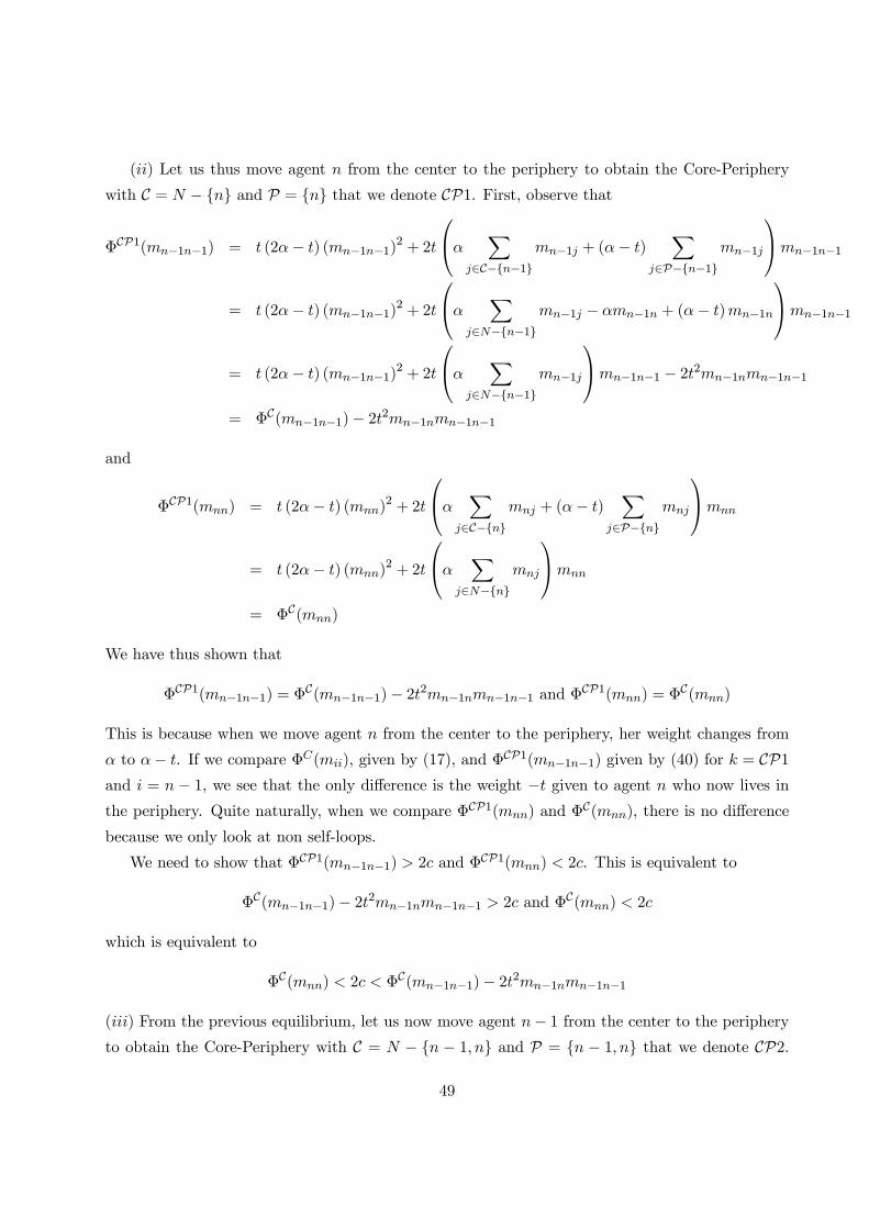
() Let us thus move agent from the center to the periphery to obtain the Core-Periphery
with C = − {} and P = {} that we denote CP1. First, observe that
ΦCP1(−1−1) = (2− ) (−1−1)2 + 2
⎛⎝X
∈C−{−1}−1 + (− )
X∈P−{−1}
−1
⎞⎠−1−1
= (2− ) (−1−1)2 + 2
⎛⎝X
∈−{−1}−1 − −1 + (− )−1
⎞⎠−1−1
= (2− ) (−1−1)2 + 2
⎛⎝X
∈−{−1}−1
⎞⎠−1−1 − 22−1−1−1
= ΦC(−1−1)− 22−1−1−1
and
ΦCP1() = (2− ) ()2 + 2
⎛⎝X
∈C−{} + (− )
X∈P−{}
⎞⎠
= (2− ) ()2 + 2
⎛⎝X
∈−{}
⎞⎠
= ΦC()
We have thus shown that
ΦCP1(−1−1) = ΦC(−1−1)− 22−1−1−1 and ΦCP1() = ΦC()
This is because when we move agent from the center to the periphery, her weight changes from
to − . If we compare Φ(), given by (17), and ΦCP1(−1−1) given by (40) for = CP1
and = − 1, we see that the only difference is the weight − given to agent who now lives inthe periphery. Quite naturally, when we compare ΦCP1() and Φ
C(), there is no difference
because we only look at non self-loops.
We need to show that ΦCP1(−1−1) 2 and ΦCP1() 2. This is equivalent to
ΦC(−1−1)− 22−1−1−1 2 and ΦC() 2
which is equivalent to
ΦC() 2 ΦC(−1−1)− 22−1−1−1
() From the previous equilibrium, let us now move agent − 1 from the center to the periphery
to obtain the Core-Periphery with C = − { − 1 } and P = { − 1 } that we denote CP2.
49

First, observe that
ΦCP2(−2−2) = ΦC(−2−2)− 22 (−2−1 +−2)−2−2
and
ΦCP2(−1−1) = ΦC(−1−1)− 22−1−1−1
We need to show that ΦCP2(−2−2) 2 and ΦCP2(−1−1) 2. This is equivalent to
ΦC(−2−2)− 22 (−2−1 +−2)−2−2 2 and ΦC(−1−1)− 22−1−1−1 2
This is equivalent to
ΦC(−1−1)− 22−1−1−1 2 ΦC(−2−2)− 22 (−2−1 +−2)−2−2
() From the previous equilibrium, let us now move agent − 2 from the center to the periphery
to obtain the Core-Periphery with C = − { − 2 − 1 } and P = { − 2 − 1 } that wedenote CP3. First, observe that
ΦCP3(−3−3) = ΦC(−3−3)− 22 (−3−2 +−3−1 +−3)−3−3
and
ΦCP3(−2−2) = ΦC(−2−2)− 22 (−2−1 +−2)−2−2
We need to show that ΦCP3(−3−3) 2 and ΦCP3(−2−2) 2. This is equivalent to
ΦC(−3−3)− 22 (−3−2 +−3−1 +−3)−3−3 2
and
ΦC(−2−2)− 22 (−2−1 +−2)−2−2 2
which is equivalent to
ΦC(−2−2)−22 (−2−1 +−2)−2−2 2 ΦC(−3−3)−22⎛⎝ X
∈P−3
⎞⎠−3−3
where P = {− 2 − 1 }.() We can continue like that until we reach a Peripheral equilibrium with C = ∅ and P = .
() From the previous equilibrium (i.e., C = {1} and P = − {1}), let us finally move agent1 from the center to the periphery to obtain the Peripheral equilibrium with C = ∅ and P = .
Observe that
ΦP(11) = ΦC(11)− 22
⎛⎝ X∈P−{1}
1
⎞⎠11
50
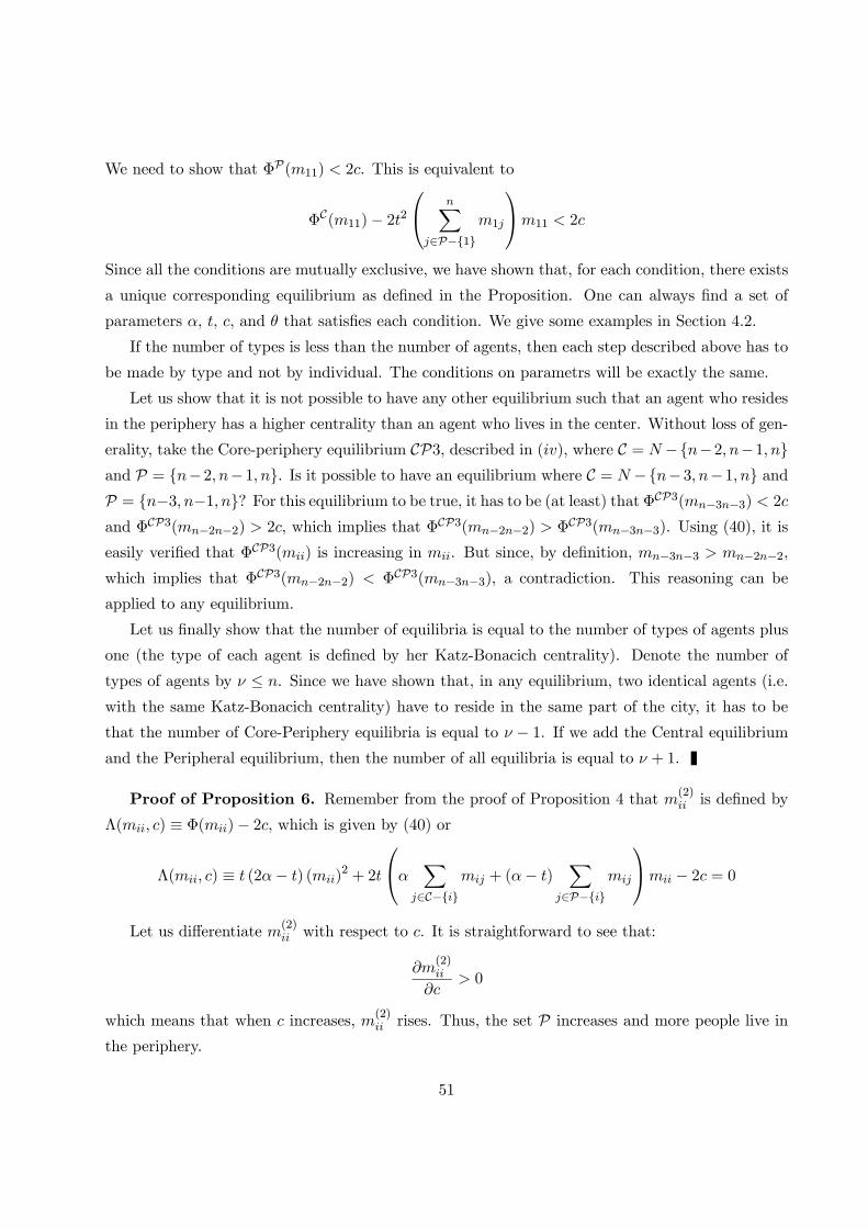
We need to show that ΦP(11) 2. This is equivalent to
ΦC(11)− 22⎛⎝ X
∈P−{1}1
⎞⎠11 2
Since all the conditions are mutually exclusive, we have shown that, for each condition, there exists
a unique corresponding equilibrium as defined in the Proposition. One can always find a set of
parameters , , , and that satisfies each condition. We give some examples in Section 4.2.
If the number of types is less than the number of agents, then each step described above has to
be made by type and not by individual. The conditions on parametrs will be exactly the same.
Let us show that it is not possible to have any other equilibrium such that an agent who resides
in the periphery has a higher centrality than an agent who lives in the center. Without loss of gen-
erality, take the Core-periphery equilibrium CP3, described in (), where C = −{−2 −1 }and P = {−2 −1 }. Is it possible to have an equilibrium where C = −{−3 −1 } andP = {−3 −1 }? For this equilibrium to be true, it has to be (at least) that ΦCP3(−3−3) 2
and ΦCP3(−2−2) 2, which implies that ΦCP3(−2−2) ΦCP3(−3−3). Using (40), it is
easily verified that ΦCP3() is increasing in . But since, by definition, −3−3 −2−2,
which implies that ΦCP3(−2−2) ΦCP3(−3−3), a contradiction. This reasoning can be
applied to any equilibrium.
Let us finally show that the number of equilibria is equal to the number of types of agents plus
one (the type of each agent is defined by her Katz-Bonacich centrality). Denote the number of
types of agents by ≤ . Since we have shown that, in any equilibrium, two identical agents (i.e.
with the same Katz-Bonacich centrality) have to reside in the same part of the city, it has to be
that the number of Core-Periphery equilibria is equal to − 1. If we add the Central equilibriumand the Peripheral equilibrium, then the number of all equilibria is equal to + 1.
Proof of Proposition 6. Remember from the proof of Proposition 4 that (2) is defined by
Λ( ) ≡ Φ()− 2, which is given by (40) or
Λ( ) ≡ (2− ) ()2 + 2
⎛⎝X
∈C−{} + (− )
X∈P−{}
⎞⎠ − 2 = 0
Let us differentiate (2) with respect to . It is straightforward to see that:
(2)
0
which means that when increases, (2) rises. Thus, the set P increases and more people live in
the periphery.
51
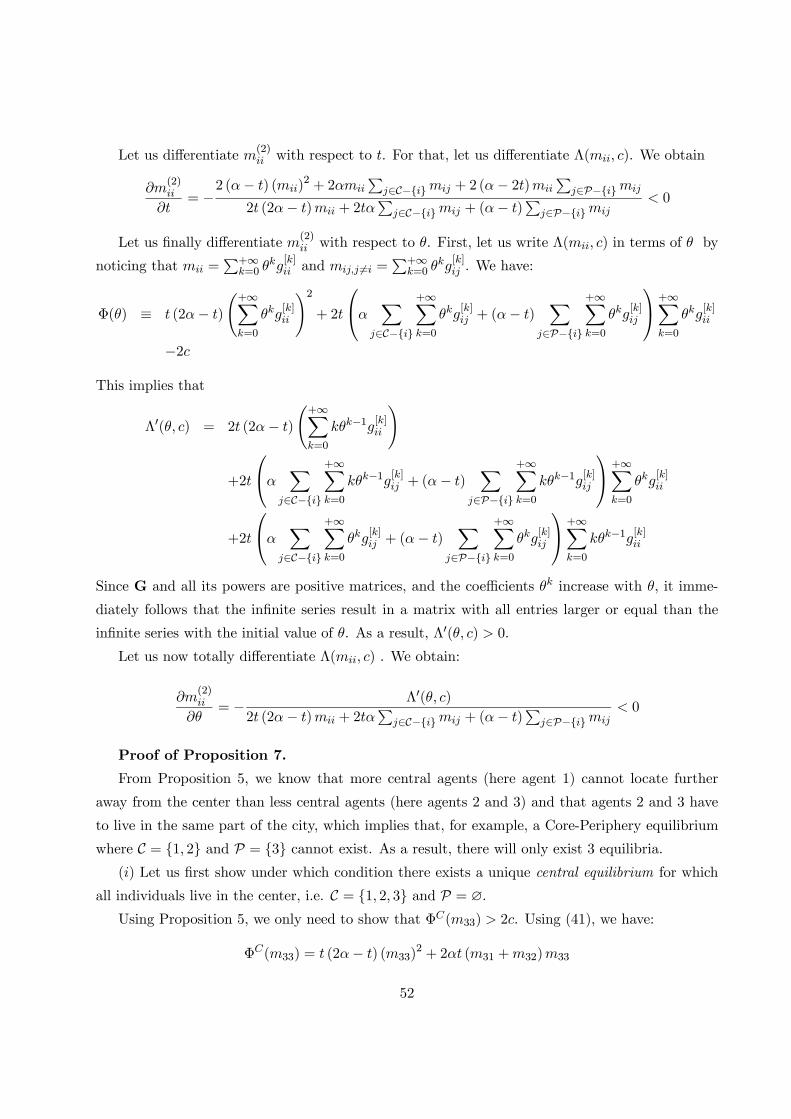
Let us differentiate (2) with respect to . For that, let us differentiate Λ( ). We obtain
(2)
= −
2 (− ) ()2 + 2
P∈C−{} + 2 (− 2)
P∈P−{}
2 (2− ) + 2P
∈C−{} + (− )P
∈P−{} 0
Let us finally differentiate (2) with respect to . First, let us write Λ( ) in terms of by
noticing that =P+∞
=0 [] and 6= =
P+∞=0
[] . We have:
Φ() ≡ (2− )
Ã+∞X=0
[]
!2+ 2
⎛⎝X
∈C−{}
+∞X=0
[] + (− )
X∈P−{}
+∞X=0
[]
⎞⎠ +∞X=0
[]
−2
This implies that
Λ0( ) = 2 (2− )
Ã+∞X=0
−1[]
!
+2
⎛⎝X
∈C−{}
+∞X=0
−1[] + (− )X
∈P−{}
+∞X=0
−1[]
⎞⎠ +∞X=0
[]
+2
⎛⎝X
∈C−{}
+∞X=0
[] + (− )
X∈P−{}
+∞X=0
[]
⎞⎠ +∞X=0
−1[]
Since G and all its powers are positive matrices, and the coefficients increase with , it imme-
diately follows that the infinite series result in a matrix with all entries larger or equal than the
infinite series with the initial value of . As a result, Λ0( ) 0.
Let us now totally differentiate Λ( ) . We obtain:
(2)
= − Λ0( )
2 (2− ) + 2P
∈C−{} + (− )P
∈P−{} 0
Proof of Proposition 7.
From Proposition 5, we know that more central agents (here agent 1) cannot locate further
away from the center than less central agents (here agents 2 and 3) and that agents 2 and 3 have
to live in the same part of the city, which implies that, for example, a Core-Periphery equilibrium
where C = {1 2} and P = {3} cannot exist. As a result, there will only exist 3 equilibria.() Let us first show under which condition there exists a unique central equilibrium for which
all individuals live in the center, i.e. C = {1 2 3} and P = ∅.Using Proposition 5, we only need to show that Φ(33) 2. Using (41), we have:
Φ(33) = (2− ) (33)2 + 2 (31 +32)33
52

Using (18), we obtain:
Φ(33) = (2− )
µ1− 2
1− 22¶2+ 2
µ
1− 22 +2
1− 22¶µ
1− 2
1− 22¶
= (1− ) (1 + )2 [2− (1− ) ]¡
1− 22¢2As a result, the condition Φ(33) 2 is equivalent to
(1− ) (1 + )2 [2− (1− ) ]
2¡1− 22¢2
() Let us now show that there exists a core-periphery equilibrium for which individuals 1 lives in the
center while individuals 2 and 3 reside in the periphery. This means that C = {1} while P = {2 3}.Using Proposition 5, the condition for the core-periphery equilibrium C = {1}, P = {2 3} to existand to be unique is given by:
ΦC(22) 2 ΦC(11)− 22 (12 +13)11
Since ΦC(33) = ΦC(22), the value of Φ
C(33) is given above. Let us determine ΦC(11) −
22 (12 +13)11. Using (41), we have:
Φ(11) = (2− ) (11)2 + 2
⎛⎝X
=−{1}1
⎞⎠11
= (2− ) (11)2 + 2 (12 +13)11
Using (18), we obtain:
Φ(11) = (2− )
µ1
1− 22¶2+ 4
µ
1− 22¶µ
1
1− 22¶
= [2 (1 + 2)− ]¡
1− 22¢2and thus
ΦC(11)− 22 (12 +13)11 = [2 (1 + 2)− ]¡
1− 22¢2 − 22µ
2
1− 22¶µ
1
1− 22¶
(43)
= [2 (1 + 2)− (1 + 4)]¡
1− 22¢2As a result, the condition ΦC(33) 2 Φ
C(11)− 22 (12 +13)11 can be written as:
(1− ) (1 + )2 [2− (1− ) ]
2¡1− 22¢2
[2 (1 + 2)− (1 + 4)]
2¡1− 22¢2
53
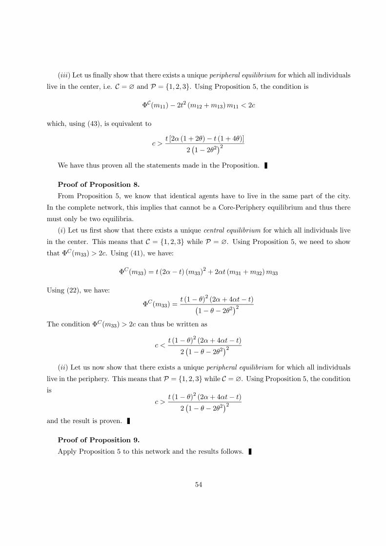
() Let us finally show that there exists a unique peripheral equilibrium for which all individuals
live in the center, i.e. C = ∅ and P = {1 2 3}. Using Proposition 5, the condition is
ΦC(11)− 22 (12 +13)11 2
which, using (43), is equivalent to
[2 (1 + 2)− (1 + 4)]
2¡1− 22¢2
We have thus proven all the statements made in the Proposition.
Proof of Proposition 8.
From Proposition 5, we know that identical agents have to live in the same part of the city.
In the complete network, this implies that cannot be a Core-Periphery equilibrium and thus there
must only be two equilibria.
() Let us first show that there exists a unique central equilibrium for which all individuals live
in the center. This means that C = {1 2 3} while P = ∅. Using Proposition 5, we need to showthat Φ(33) 2. Using (41), we have:
Φ(33) = (2− ) (33)2 + 2 (31 +32)33
Using (22), we have:
Φ(33) = (1− )2 (2+ 4− )¡
1− − 22¢2The condition Φ(33) 2 can thus be written as
(1− )2 (2+ 4− )
2¡1− − 22¢2
() Let us now show that there exists a unique peripheral equilibrium for which all individuals
live in the periphery. This means that P = {1 2 3} while C = ∅. Using Proposition 5, the conditionis
(1− )2 (2+ 4− )
2¡1− − 22¢2
and the result is proven.
Proof of Proposition 9.
Apply Proposition 5 to this network and the results follows.
54