Social Welfare, Income Inequality, and Tax Progressivity: A Primer on Modern Economic Theory and Evidence

Jon Bakija Williams College

jbakija@williams.edu October 2013

Abstract: The economic literature on “optimal income taxation” addresses the question of how to design tax and transfer policy so as to maximize “social welfare,” which is some function of the well-being of all members of society. It clarifies how the social-welfare-maximizing policy depends on one’s philosophy of distributive justice, and on empirical evidence about the behavioral response to incentives, and thus provides a systematic way of evaluating the tradeoff between equity and efficiency. Here, I explain the key insights of the optimal income taxation literature in a way that should be accessible to those with a familiarity with introductory economics. Next, I present evidence on inequality in economic well-being the U.S., how it has been changing over time, and to what extent tax and transfer policies reduce inequality. I then consider different possible explanations for rising inequality, and discuss why different explanations may have different implications the efficiency costs of taxation.

Parts of this paper draw on lengthier treatments of these issues included in Slemrod and Bakija (forthcoming), and Bakija, Cole, and Heim (2012).

I. Social Welfare, the Tradeoff between Equity and Efficiency, and Optimal Income Taxation: Theory

As Arthur Okun (1975) memorably put it, taxing the better-off to finance transfers to the worse-off is like “carrying water in a leaky bucket.” The leak represents the administrative costs of the tax and transfer system, and the deadweight losses caused by the fact that taxes and transfers distort incentives, causing people to change their behavior in an effort to reduce their tax bill or increase the transfer received. Different philosophies of distributive justice lead to different conclusions about how much of a leak we should be willing to accept before we stop carrying further buckets. The economic literature on “optimal income taxation” provides a systematic way of thinking about this question, by positing that decisions about tax and transfer policy should be made so as to maximize “social welfare,” which is some function of the well-being of all members of society. It provides an integrated framework for evaluating policy that can flexibly incorporate a variety of philosophies of distributive justice, while taking into account the fact that taxes and transfers have costs in terms of economic efficiency. Economist James Mirrlees did pioneering work on the theory of optimal income taxation in the early 1970s, and was awarded a Nobel Prize in economics for this and other work in 1996. More recently, economists such as Emmanuel Saez at the University of California, Berkeley, 2009 winner of the John Bates Clark medal (given to “the American economist under the age of forty who is judged to have made the most significant contribution to economic thought and knowledge”), have advanced research on optimal income taxation in a number of ways, especially in terms of identifying parameters that summarize the responsiveness of behavior to incentives which can be estimated empirically, and then showing how these can be combined with ethical judgments that must come from philosophy, and translated into policy recommendations.1

To begin, let’s remind ourselves what “economic efficiency” means. One possible measure of social welfare is “economic surplus,” also known as “money-metric utility,” which represents the sum of all dollar-valued “net benefits” in society. So for example, if, given my income, circumstances, and tastes, I am willing to pay $5 for my first cup of coffee in the morning, and if I only have to pay a price of $2 for it, the difference, $3, is a net benefit to me measured in dollars, and that is my economic surplus from that cup of coffee. To the extent that the price of that cup of coffee exceeds the marginal cost of making it, that provides some economic surplus to the producers too. Economic activity might create benefits or impose costs on other people not directly involved in the market transaction, and that would be accounted for in economic surplus too – so for example, in the case of an “externality” such as pollution, the dollar-valued harm from the pollution would represent a loss of economic surplus. In the absence of “market

1 Mirrlees (1971) is a seminal contribution to the theory of optimal income taxation. Weisbach (2003) offers a brief and accessible illustration of the basic idea. Diamond and Saez (2011) and Mankiw, Weinzierl, and Yagan (2009) provide more advanced, but still accessible discussions of theory and evidence on optimal income taxation and its policy implications, each from somewhat different perspectives. Kaplow (2008) offers a book-length argument that the ideas discussed here represent the unifying conceptual framework for thinking about all normative questions in economics. Boadway (2011) offers a discussion and critique of Kaplow.

1

failures” such as externalities, free markets are economically efficient, in the sense of maximizing economic surplus, because consumers and producers will do all things for which the dollar-valued benefits exceed the dollar-valued costs to them, and none of the things for which the dollar-valued costs exceed the dollar-valued benefits to them.

The optimal income tax literature is motivated by the recognition that economic surplus is a highly imperfect concept of social welfare. An influential alternative concept of social welfare is utilitarian social welfare, which is the sum of individual utilities in society. Whereas economic efficiency is about maximizing the sum of money metric utilities (economic surplus, or well-being measured in dollars), utilitarianism is about maximizing the sum of utilities, denominated in units of happiness rather than in dollars. While that might seem like a subtle distinction, the implications for public policy can be wildly different under utilitarianism compared to an ethic that only values economic efficiency. Utilitarianism is a more general and flexible concept of social welfare than economic surplus, in that that allows for the plausible possibility that there is diminishing marginal utility – that is, an additional dollar of well-being translates to a larger improvement in utility for someone who is economically worse-off compared to someone who is economically better-off. So for example, an additional $100 might enable an affluent family to buy a few more magazine subscriptions, but it might enable a poor family to avoid starvation.

Empirical evidence on how people respond to risky situations (for example, buying insurance, or demanding a risk premium to be willing to hold a risky asset) are consistent with the idea of diminishing marginal utility.2 In principle, one can estimate how quickly marginal utility diminishes as income increases for a given individual by observing how their behavior changes in response to risky situations, the degree to which they try to smooth their consumption over time, and so forth. We cannot scientifically estimate how levels of utility differ across people, though. There is no way to objectively measure and compare the absolute level of joy or pain across people. So to make a utilitarian social welfare analysis operational, we need to make some assumptions about the nature of each person’s utility function that are potentially testable (e.g., the curvature of each individual’s the utility function), and some assumptions that not empirically testable (e.g., how the level of utility compares across individuals). Alternatively, we might think of assumptions about the latter as ethical judgments about how much each person’s utility should count when adding up social welfare.

Utilitarianism is often criticized on the grounds that there is no objective way to make inter-personal comparisons of utility. However, it is also well-recognized in economics that evaluating policy based on whether or not it is “economically efficient” implicitly involves a similar problem, unless we confine ourselves only to recommending actual Pareto improvements (changes that make at least one person better off without harming anyone else). Actual Pareto improvements are so rare as to make the concept almost completely useless as a guide to policy. If we instead evaluate a policy change based on whether it is “economically efficient” in the sense of increasing economic surplus, then there may be both winners and losers from the policy, and all we can say is that the gains to the winners are larger than the

2 An explanation of the connection between behavior in response to risk and diminishing marginal utility is provided in Chapter 12 of Gruber (2011).

2

losses to the losers when measured in dollars. If we claim that a policy change that is not a Pareto improvement is “good” or “social welfare enhancing” because it has a net positive impact on economic surplus, then our evaluation implicitly involves an inter-personal comparison of well-being, and that comparison relies on a metric of well-being which ignores diminishing marginal utility.3

Leaving aside debates about interpersonal comparability of utility for now, let’s consider what the principle of diminishing marginal utility might imply if our goal was to maximize utilitarian social welfare. Figure 1 below depicts a hypothetical relationship between an individual’s well-being measured in dollars (economic surplus) on the horizontal axis, and his or her well-being measured in utility on the vertical axis, under the intuitively plausible assumption that there is diminishing marginal utility. In the diagram, the marginal utility from another dollar of well-being is the slope of the utility function – that is, the change in utility associated with a $1 change in well-being. The utility curve starts out steep, meaning that a small increase in well-being measured in dollars is associated with a big increase in well-being measured in utility – that is, marginal utility is large when well-being measured in dollars is small. As economic surplus gets larger and larger, the utility curve gets flatter, meaning its slope gets smaller. Thus, when well-being measured in dollars is higher, a given increase in well-being measured in dollars is associated with a smaller increase in utility – that is, marginal utility tends to be smaller for people with more economic surplus (who tend to have higher incomes).

The potential for redistribution to raise the sum of utilities in society should be apparent

from figure 1. If we were somehow able to do something that made someone who is on the right-hand side of the figure (a higher-income person) worse off by $1, and that enabled us to

3 Friedman (1997, chapter 15) provides an accessible discussion of these issues.

Utility

Economic Surplus ($)

Utility Function

Figure 1 – A Hypothetical Relationship between Well-Being Measured in Dollars and Well-Being Measured in Utility

3

make someone on the left-hand side of the figure (a lower-income person) better off by $1, it would increase the utility of the lower-income person by more than it reduces the utility of the higher-income person, and so would increase the sum of utilities in society. A utilitarian believes that the ethical goal of a society should be to maximize social welfare, and that social welfare is the sum of individual utilities in the society. So a utilitarian would support the particular redistribution just described.

In the utilitarian framework, one needs to take into account that redistributing from rich to poor requires taxes and transfers that generally reduce incentives to engage in productive activity. That is part of what creates the “leak in the bucket.” The deadweight loss (net reduction in aggregate economic surplus in society) from taxation means that redistribution from rich to poor makes the rich worse off by more than it makes the poor better off when measured in dollars. To a utilitarian, this must be weighed against the gains in utility from redistributing from people with low marginal utility to people with high marginal utility described earlier.

One way to do this would be to make assumptions about the functional forms of peoples’ utility functions, measure their wages, and work out the social-welfare maximizing tax rates and transfers. The basic idea is that a utility function that includes consumption and leisure implies a particular labor supply curve for that individual, and once you know the individual’s utility function and labor supply curve, you can derive how hours worked, tax revenues, and the transfers financed by tax revenues change when tax rates change, which gives you everything you need to solve the problem. The utilitarian would then favor the combination of tax rates and transfers that maximizes the sum of utilities in society. Weisbach (2003) illustrates the basic idea with a simple example, although the example is not meant to be empirically realistic, but rather mathematically convenient so as to illustrate the principles involved. Actually determining the nature of peoples’ utility functions would be an extremely difficult empirical and philosophical challenge, but economists have done a great deal of empirical research that contributes to piecing together this puzzle.

In what follows, I provide a simplified way to think about the question that helps convey the basic issues involved, and points out key factors that influence where the social-welfare maximizing point might lie, in a way that is more transparent than Weisbach’s example. Even though some of these factors may be difficult or impossible to pin down empirically, some are indeed amenable to empirical investigation, and others are arguably matters of ethical reasoning – this kind of analysis at least helps clarify where the ethical judgments come into play and how they matter.

To illustrate what factors the social welfare maximizing solution depends on, let’s consider a simple example where we are going to tax the labor income of one rich person, and then transfer the resulting tax revenue directly to a poor person as a lump-sum grant. In this simplified example, we only need to worry about the deadweight loss caused by taxing the rich person, because lump-sum transfers cause no deadweight loss.4 To keep things simple, we will

4 “Lump-sum” means that the tax or transfer is a fixed amount regardless of what the person does -- there is no way to change one’s behavior in order to reduce or increase the amount of a lump-sum tax or transfer. For an explanation of why lump-sum taxes and transfers do not involve deadweight loss, see Rosen and Gayer (2008, pp. 331-340) and Bakija (2011).

4

also assume that the demand for the rich person’s labor is perfectly elastic at his pre-tax wage. This is a non-trivial assumption, because if demand for the labor of the rich is not perfectly elastic, then some of the burden of the tax on them will be shifted onto someone else, and we’d have to take that into account too – to the extent the burden of taxes on the rich are shifted onto other people who are less well-off, that would reduce the optimal amount of redistributive taxation in a utilitarian framework, because the taxation may be hurting some of the people we are intending to help. This is part of what opponents of high tax rates on the rich have in mind when they lament that taxing the “job creators” ends up hurting others. But starting with the assumption of perfectly elastic demand for the labor of the rich enables us to illustrate the basic ideas simply by confining our attention to just two people.

Under the assumptions described above, figure 2 depicts the effects of a labor income tax on the labor supply and economic surplus of the rich person. To begin, suppose that we are starting from a situation with no taxes or transfers, and we are considering whether to impose a tax on the labor income of the rich person at a rate of t1. This puts a wedge between the demand for the rich person’s labor and the supply equal to t1W, where W is the rich person’s pre-tax wage (in other words, t1W is the tax per hour worked expressed in dollars). The revenue from the tax will be transferred entirely to the poor person in a lump-sum fashion. Each letter a through f represents the area of the shape that the letter labels (the areas are measured in dollars).

A tax at rate t1 causes the rich person to reduce hours worked from H0 to H1. It collects tax revenue equal to a+b, and that is how much we have available to transfer to the poor person, and thus how much better-off we can make the poor person, measured in dollars. However, the rich person is made worse off by more than that when measured in dollars: a+b+c. The difference (c) arises due to the deadweight loss of taxation – the loss of economic surplus that occurs because people change their behavior when their incentives are distorted by taxes. By reducing hours worked from H0 to H1, the rich person’s before-tax income is reduced by c+f. This is partly compensated by a gain in leisure, but the extra leisure is only worth f to the rich person (recall that the area under the supply curve represents the opportunity cost, or value of the next best alternative, for the activity in question – in this case, the opportunity cost of working is the value of the leisure that is foregone). The difference between the lost pre-tax income and the value of the leisure gained is c, and that is the deadweight loss or “excess burden” (hidden cost) of taxation. Reducing hours worked from H0 to H1 reduces the rich person’s tax bill by more than the deadweight loss, which is why it makes sense to do this from his or her individual perspective. But the tax bill that the rich person avoids just represents transfer, not a net change in aggregate economic surplus for the society (avoiding the tax is a gain to the rich person, but an equal loss to the poor person who would otherwise have received a bigger transfer). The deadweight loss, by contrast, is a net loss of economic surplus to society. It represents the amount by which the dollar value of income between H0 and H1 that we are losing had exceeded the dollar value leisure that we get instead.

5

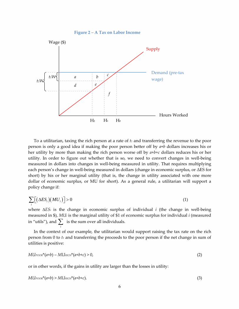
To a utilitarian, taxing the rich person at a rate of t1 and transferring the revenue to the poor

person is only a good idea if making the poor person better off by a+b dollars increases his or her utility by more than making the rich person worse off by a+b+c dollars reduces his or her utility. In order to figure out whether that is so, we need to convert changes in well-being measured in dollars into changes in well-being measured in utility. That requires multiplying each person’s change in well-being measured in dollars (change in economic surplus, or ΔES for short) by his or her marginal utility (that is, the change in utility associated with one more dollar of economic surplus, or MU for short). As a general rule, a utilitarian will support a policy change if:

( )( ) 0i i

iES MU ∆ > ∑ (1)

where ∆ESi is the change in economic surplus of individual i (the change in well-being measured in $), MUi is the marginal utility of $1 of economic surplus for individual i (measured in “utils”), and

i∑ is the sum over all individuals.

In the context of our example, the utilitarian would support raising the tax rate on the rich person from 0 to t1 and transferring the proceeds to the poor person if the net change in sum of utilities is positive:

MUPOOR*(a+b) – MURICH*(a+b+c) > 0, (2)

or in other words, if the gains in utility are larger than the losses in utility:

MUPOOR*(a+b) > MURICH*(a+b+c). (3)

Demand (pre-tax wage)

Supply Wage ($)

Hours Worked H0 H1 H2

c b a

e d

t1W

Figure 2 – A Tax on Labor Income

f

t2W

6

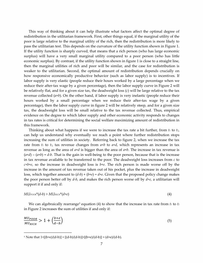
This way of thinking about it can help illustrate what factors affect the optimal degree of

redistribution in the utilitarian framework. First, other things equal, if the marginal utility of the poor is large relative to the marginal utility of the rich, then the redistribution is more likely to pass the utilitarian test. This depends on the curvature of the utility function shown in Figure 1. If the utility function is sharply curved, that means that a rich person (who has large economic surplus) will have a very small marginal utility compared to a poor person (who has little economic surplus). By contrast, if the utility function shown in figure 1 is close to a straight line, then the marginal utilities of rich and poor will be similar, and the case for redistribution is weaker to the utilitarian. Second, the optimal amount of redistribution depends crucially on how responsive economically productive behavior (such as labor supply) is to incentives. If labor supply is very elastic (people reduce their hours worked by a large percentage when we reduce their after-tax wage by a given percentage), then the labor supply curve in Figure 2 will be relatively flat, and for a given size tax, the deadweight loss (c) will be large relative to the tax revenue collected (a+b). On the other hand, if labor supply is very inelastic (people reduce their hours worked by a small percentage when we reduce their after-tax wage by a given percentage), then the labor supply curve in figure 2 will be relatively steep, and for a given size tax, the deadweight loss will be small relative to the tax revenue collected. Thus, empirical evidence on the degree to which labor supply and other economic activity responds to changes in tax rates is critical for determining the social welfare maximizing amount of redistribution in this framework.

Thinking about what happens if we were to increase the tax rate a bit further, from t1 to t2, can help us understand why eventually we reach a point where further redistribution stops increasing the sum of utilities in society. Referring back to figure 2, when we increase the tax rate from t1 to t2, tax revenue changes from a+b to a+d, which represents an increase in tax revenue as long as the area of a+d is bigger than the area of a+b. The increase in tax revenue is (a+d) – (a+b) = d-b. That is the gain in well-being to the poor person, because that is the increase in tax revenue available to be transferred to the poor. The deadweight loss increases from c to c+b+e, so the increase in deadweight loss is b+e. The rich person is made worse off by the increase in the amount of tax revenue taken out of his pocket, plus the increase in deadweight loss, which together amount to (d-b) + (b+e) = d+e. Given that the proposed policy change makes the poor person better off by d-b, and makes the rich person worse off by d+e, a utilitarian will support it if and only if:

MUPOOR*(d-b) > MURICH*(d+e) (4)

We can algebraically rearrange5 equation (4) to show that the increase in tax rate from t1 to t2

in Figure 2 increases the sum of utilities if and only if:

𝑀𝑈𝑃𝑂𝑂𝑅𝑀𝑈𝑅𝐼𝐶𝐻

> 1 + �𝑏+𝑒𝑑−𝑏

� (5)

5 Note that 1+[(b+e)/(d-b)] = [(d-b)/(d-b)]+[(b+e)/(d-b)] = (d+e)/(d-b).

7

As noted above, (b+e) is the increase in deadweight loss caused by the raising the tax rate

from t1 to t2, and (d-b) is the increase in tax revenue caused by raising the tax rate from t1 to t2. Their ratio, [(b+e)/(d-b)] is known as the marginal deadweight loss per dollar of revenue raised, abbreviated MDWL / MR. This is an extremely useful summary measure of how leaky the bucket is. It represents the amount of deadweight loss caused by raising one more dollar of tax revenue. The right-hand-side of the equation (5) above is 1 + MDWL / MR, and is sometimes called the “marginal cost of public funds.” It represents how much worse off we make the (rich) taxpayer, in dollars, when we collect $1 more in tax revenue from him or her. So in this example, further redistribution from rich to poor is only desirable from a utilitarian perspective if the ratio of the marginal utility of the poor to the marginal utility of the rich is at least as large as 1 + MDWL / MR. So for example, if collecting $1 of tax revenue from a rich person makes the rich person worse off by $1.50, then doing so and transferring the $1 to a poor person will only increase utilitarian social welfare if a dollar is worth more than 1.5 times as much in terms of utility to the poor person as to the rich person.

This formula can help illustrate why we eventually reach an “optimum” level of redistribution in the utilitarian framework, beyond which further redistribution would reduce the utility of the rich more than it would raise the utility of the poor. Looking at figure 2, it should be apparent that each time we raise the tax rate another notch, b+e, the marginal change in deadweight loss, gets larger, and d-b, the marginal change in revenue, gets smaller. Thus, the marginal deadweight loss per dollar of additional revenue raised rises as the tax rate rises. In the context of Okun’s metaphor, each successive bucket that we carry from rich to poor will be a little bit leakier than the previous one. In addition, looking at figure 1, it should be apparent that as we redistribute more and more from the rich to the poor, their marginal utilities will move closer to each other, so that MUPOOR / MURICH gets smaller and approaches 1 as we get closer to equality. In the context of Okun’s metaphor, with each successive bucket that we carry, the rich person gets a little thirstier and the poor person gets a little less thirsty. Thus, as we keep raising the tax rate and redistributing more and more, the left hand side of equation (5) gets smaller, and the right hand side of equation (5) gets larger, until we get to the point where they are just equal. That is the amount of redistribution that maximizes utilitarian social welfare. At that point, any further redistribution would reduce the utility of the rich more than it increases the utility of the poor. Other things equal, when behavior such as labor supply is more elastic with respect to incentives, then MDWL / MR will be larger, and the social welfare maximizing tax rate will be lower.

The simplified analysis above is of course just an approximation. One reason is that the marginal utility of each person is changing continuously with each dollar of redistribution, so using a fixed value of MU in any of the equations above will not get things exactly right. Still, for reasonably small changes in tax rate, using the MU that applied at the beginning tax rate and holding it constant will usually come very close to giving you the right answer. Another reason is that the deadweight loss measured from figure 2 will also just be an approximation as long as a tax change has both substitution effects and income effects. For technical reasons, measuring deadweight loss accurately requires isolating the change in economic behavior that

8

is due solely to the substitution effect, and removing any changes arising from the income effect.6

Saez and Stantcheva (2013) show how this basic framework can be adapted to accommodate virtually any philosophy of distributive justice, and can even accommodate combinations of the different philosophies. The key insight is to replace the marginal utilities (MU) in the example above with “marginal social welfare weights,” which represent the ethical value that we assign to dollar-valued gains and losses to different people. The idea is that in virtually any philosophy of distributive justice, we ought to care about the dollar-valued costs and benefits of achieving our ethical goals, but we also ought to weight dollar-valued costs and benefits to different people differently depending on the ethical value of gains and losses to those people. Here are a few examples.

Philosopher John Rawls argued that public policy should be designed so as to maximize the well-being of the worst-off person in society. In the Saez and Stantcheva framework, that would correspond to evaluating whether a policy change is an improvement by multiplying dollar-valued gains and losses to the worst-off person in society by a marginal social welfare weight of one, and multiplying dollar-valued gains and losses to all other members of society by a marginal social welfare weight of zero. In our stylized example above, that would mean raising taxes on the rich person to the revenue maximizing rate (i.e., going to the peak of the Laffer curve, but no further). At that point, any further increases in the tax rate would reduce tax revenue, and therefore the transfer to the poor person, making the poor person worse off.

“Luck egalitarian” philosophers such as Ronald Dworkin and John Roemer argue that public policy should do as much as possible to compensate people for the consequences of bad luck, but should also do as little as possible to compensate people for the consequences of bad effort and bad choices. In the Saez and Stantcheva framework, that would correspond to assigning large marginal social welfare weights to dollar-valued gains and losses of people who are badly off through no fault of their own, and smaller marginal social welfare weights to dollar-valued gains and losses of people who are well-off due to good luck, or badly off due to their own choices and effort. The practical implications of this might be, for example, to particularly favor redistribution that takes the form of government provided or subsidized insurance against unfortunate circumstances, such as disability or genetic health conditions, or providing high-quality early childhood education to children unlucky enough to be born into disadvantaged home. Saez and Stantcheva also conduct a survey where they ask a sample of U.S. citizens detailed questions about hypothetical redistributive policies, and the results suggest that many Americans do favor taking account factors such as luck, effort, and dessert when evaluating policy. So for example, survey respondents were given four examples of individuals with a $15,000 of income, one of whom is disabled, one of whom is unemployed and cannot find a new job, and two of whom have no job and are not looking for one because they prefer not to work, and asked which were most deserving of $1,000 of government transfer, allowing for ties. About 95 percent said one or both of the first two people were more deserving of an increased transfer. They also offered a scenario where two people earn equal incomes and pay equal taxes, but one works twice the number of hours at half the wage, and asked which person was

6 See Bakija (2011b) and Rosen and Gayer (2008) for an explanation.

9

more deserving of a $1,000 tax cut. 43 percent said the harder working person was more deserving of the tax cut, while 54 percent said they were equally deserving of a tax cut.

Mankiw (2010) argues that a libertarian principle for evaluating whether a policy change is an improvement would be whether it causes tax payments to more closely match benefits received from the government (hearkening back to the “benefit principle” advocated by Adam Smith). Saez and Stantcheva show that this principle can be accommodated in their framework by assigning larger marginal social welfare weights to dollar-valued gains and losses of people whose tax payments are farther above the benefits they receive from the government, and by assigning smaller marginal social welfare weights to people whose tax payments are farther below benefits received from the government.

Saez and Stantcheva also show how “horizontal equity” concerns can be accommodated in their framework. Horizontal equity is the principle that it is unfair to impose different tax burdens on different people who have the same ability to pay taxes. This is a kind of non-discrimination principle, where it is considered unethical to tax people with equal capacity to pay tax differently because of irrelevant characteristics such as tastes, or ethnicity, or height. Public finance economists have long recognized that this captures an important element of popular attitudes towards fairness in taxation, and for a long time the standard treatment of equity questions in public finance economics textbooks has given weight to both utilitarian concerns (which were considered part of “vertical equity,” the question of how people with differing abilities to pay taxes should be treated) and to horizontal equity concerns.7 Some policy implications of a pure utilitarian analysis seem to conflict with the principle of horizontal equity. For instance, under some circumstances, imposing higher taxes on people with certain immutable characteristics (known as “tags”) that are positively correlated with income, such as height, and transferring the proceeds to people without those characteristics, would increase utilitarian social welfare. That is because the policy would, on average, transfer resources from better-off people to worse-off people, and it would do so in a way that causes no deadweight loss, because the redistribution is based on immutable characteristics. Thus there is no opportunity to change behavior in order to avoid the tax or to increase the transfer received. Mankiw and Wienzierl (2010) argue that many people would consider taxes and transfers based on seemingly irrelevant characteristics such as height unfair, and that this represents a fundamental problem with utilitarianism. Saez and Stantcheva reply that it just suggests people care about more than one ethical principle at the same time, and they show that concern for multiple ethical principles can easily be accommodated in their framework. For example, utilitarian marginal social welfare weights (which are proportional to marginal utilities) can be multiplied by factors that put greater weight on gains and losses of utility to people who are suffering from horizontal inequity.

II. Facts about Income Inequality, Taxes, and Transfers in the U.S.

One of the most dramatic developments in the U.S. economy in recent decades has been the tremendous rise in the share of income going to people at the very top of the income

7 Musgrave (1990) discusses the intellectual history of horizontal equity concerns in economics.

10

distribution. The gray line in the top panel of figure 3 depicts, for the years 1913 through 2011, the percentage of total pre-tax market income in the U.S. going to households in the top 1 percent of the income distribution, calculated by Thomas Piketty of the Paris School of Economics and Emmanuel Saez of the University of California at Berkeley. It represents the top 1 percent’s share of the following: gross income reported on personal income tax returns (including realized capital gains – that is, the difference between the sales price and purchase price of an asset, such as a stock), plus an estimate of what that income would be for those not filing tax returns, less any government transfers included in gross income such as social security or unemployment insurance. By this measure, the minimum and average incomes of households in the top 1 percent in 2011 were $367,000 and just under $1 million, respectively.8

The top 1 percent’s share of pre-tax market income has followed a U-shaped pattern since the early 20th century. It fell from a peak of 24 percent in 1928 to about 10 percent by the mid-1950s, and stayed around this level through the mid-1970s, when it briefly dipped below 9 percent. It then began to rise dramatically, eventually reaching about 24 percent again by 2007, fell temporarily to 18 percent during the recession year of 2009, but had already rebounded to about 20 percent by 2011, which is still higher than in any year between 1930 and 1998.

The dashed line in the top panel of figure 3 shows an alternative estimate of the top 1 percent’s income share, based on the Congressional Budget Office (CBO) measure of pre-tax market income. This is similar to Piketty and Saez’s measure (including realized capital gains), but accounts for some additional kinds of market income, the most important being employer-provided health insurance and pension contributions. CBO’s data suggests a roughly similar degree of inequality and a similar pattern of changes over time, at least since 1979 when the CBO data start. The CBO measure is a bit lower in recent years because CBO’s data ends in 2009 (thus missing the 2010-11 rebound) and because, compared to other market income, employee benefits are less concentrated in the top 1 percent and growing faster over time. But this does not change the picture very much.

The solid black line in the top panel of figure 3 shows the top one percent’s share of the Piketty-Saez measure of income excluding capital gains. Comparing this to the gray line demonstrates that almost all of the recent volatility in the top 1 percent’s income share has been due to fluctuations in realized capital gains, mostly reflecting the wild swings in the stock market. Excluding capital gains, there is evidence of an even steadier upward trend in the share of pre-tax market income going to the top 1 percent since the 1970s, which thus far shows little sign of abating. The top 1 percent’s share of this measure of income rose from less than 8 percent in the late 1970s to more than 17 percent in 2011.

8 Piketty and Saez (2003, updated 2013, Table A5).

11

12

The bottom panel of figure 3 demonstrates that since 1979, average real (inflation-adjusted) pre-tax market income per household, as measured by CBO, has grown much faster the higher one goes in the income distribution. In the top 1 percent of the income distribution, it grew by 268 percent between 1979 and 2007. Despite falling during the early part of the recent recession (again mostly because of a temporary dip in capital gains realizations), it was still 134 percent higher in 2009 than it was in 1979. In the rest of the top quintile (or fifth) of the income distribution, income growth was strong but less dramatic, at 81 percent from 1979 to 2007 and 55 percent from 1979 through 2009. In the second-highest quintile, average real pre-tax market income grew by 45 percent between 1979 and 2007, and by 2009 was still 37 percent higher than in 1979. For the bottom 60 percent of the income distribution, the comparable figures were 22 percent and 8 percent, respectively.

While the distribution of pre-tax market income in the U.S. is very unequal, and growing more unequal over time, the inequality is mitigated to some extent by tax policy. Table 1 presents the Urban-Brookings Tax Policy Center’s estimates of the distribution of federal taxes in 2013. Column 2 of table 1 indicates that the distribution of federal taxes as a whole is quite progressive, meaning that average tax rates (taxes as a percentage of income) are higher for upper-income people than for lower-income people. with average tax rates rising from 1.8 percent for people in the lowest fifth of the income distribution, to 15.4 percent in the middle fifth, and then to 35.7 percent in the top percentile. Thus, the notion that by taking advantage of loopholes, tax shelters, and the like, the tax burden of upper-income people is a smaller share of their income than it is for everyone else, is far from the truth, at least on average.

13

The estimates in the third column of table 1 indicate that the federal personal income tax in particular is highly progressive. Average income tax rates range from -7.3 percent of cash income in the bottom quintile, to 4.3 percent in the middle, to 25.2 percent in the top percentile. The negative average tax rate figures for the bottom quintile are due to the refundable portions of the earned income tax credit as well as the child credit. For many people in this income group, on net they get payments from the federal government through the personal income tax. Comparing the estimates for overall federal taxes (in column 2) and personal income taxes (in column 3) makes clear that income taxation accounts for nearly all of the progressivity of the federal tax system; most other federal taxes are either proportional or regressive in their distribution.

Columns 5 and 6 of table 3.2 show the Tax Policy Center’s projection of the percentage of total cash income that people in each part of the income distribution will receive in 2013, and their estimates of the percentage of the total federal tax burden that is borne by people in each part of the income distribution. The share of taxes is higher than the share of income throughout the top decile, the same as the share of income for the bottom half of the top quintile, and lower than the share of income for each of the bottom four quintiles, another indicator of tax progressivity. The top 1 percent is estimated to bear 29.3 percent of the overall federal tax burden, which is the combined effect of progressive taxes and receiving such a large share (17.4 percent) of all income.

Figure 4 illustrates how average federal tax rates changed between 1979 and 2009 for people at different points in the income distribution, based on an analysis by the CBO. The most dramatic changes in average federal tax rates since 1979 occurred at the top of the income distribution. The average federal tax rate in the top income percentile fell from 35.1 percent in 1979 to a low of 24.6 percent in 1986 as a result of the Reagan-era tax cuts, rebounded to 35.3 percent in 1995 after an increase in the top tax rate during the Clinton administration, fell a bit to 32.4 percent by 2000 partly due to a 1997 cut in the capital gains tax rate, and then dropped more significantly to 28.9 percent by 2009 mainly because of tax cuts enacted during the George W. Bush administration. Table 1 suggests that the increase in the top federal income tax rate from 35 percent to 39.6 percent, enacted at the beginning of 2013, has restored the average federal tax rate on the top one percent to about where it was in the mid-1990s.

In the rest of the income distribution, federal average tax rates changed relatively modestly between 1979 and 2000, but declined substantially between 2000 and 2009. In the bottom quintile, the average federal tax rate fell from 7.5 percent in 1979 to 6.8 percent in 2000, and then plummeted to 1.0 percent in 2009. In the middle quintile, the average federal tax rate fell from 18.9 percent in 1979 to 16.5 percent in 2000, and then dropped to just 11.1 percent by 2009. For the top 5 percent outside of the top 1 percent, the average federal tax rate was 27.1 percent in 1979 and 27.9 percent in 2000, but had dipped to 24.1 percent by 2009. Average federal tax rates in the middle and bottom of the income distribution were unusually low in 2009 partly because of temporary stimulus measures that have since expired. Table 1 suggests that average federal tax rates had rebounded a bit in the middle and bottom of the distribution by 2013, largely due to the expiration of stimulus measures. But average federal tax rates were still generally at least a couple of percentage points lower in 2013 compared to 2000 in all parts of the income distribution outside the top one percent, mainly reflecting the fact that most of the George W.

14

Bush era tax cuts were made permanent starting in 2013 for all but the highest-income taxpayers.

15

Another major way that government influences income inequality is through transfers. Table 2 displays CBO estimates of the average annual value per household of federal and state government transfers during 2004 through 2009, at different points in the income distribution. The overwhelming majority of such transfers go to the elderly and disabled. Social Security and Medicare benefits, which go exclusively to the elderly, disabled, and dependent survivors of deceased workers, accounted for 71 percent of the value of transfers. Medicaid, the federal-state program that provides health insurance for low-income people, comprised another 15 percent of transfers. The elderly and disabled accounted for about two-thirds of Medicaid expenditures in 2009, even though they only represented a quarter of the people covered by Medicaid.9 A major reason is that Medicare does not cover long-term care (such as an extended stay in a nursing home), which is often so expensive that it forces elderly and disabled people who need it into poverty, qualifying them for Medicaid. The Medicaid program also provides health insurance to large numbers of children -- in 2012, about one-third of all children in the U.S. were enrolled in Medicaid, up from one-quarter in 2007, with the recent increase due mainly to the recession, but they account for a small share of Medicaid spending because of their relatively low health care costs.10 All other transfers, including unemployment insurance benefits, food stamps, welfare benefits, and many other programs, accounted for just 14 percent of transfers; in the bottom quintile, these averaged about $1,800 per household. This is higher than usual because the period 2004-2009 includes the beginning of the worst recession in the U.S. since the Great Depression, which temporarily increased the share of people receiving unemployment benefits, food stamps, etc.

Table 2 shows that the average dollar values of government transfers per household do not vary greatly across the income distribution. The poorest quintile actually receives the smallest average transfer per household ($7,700), while the second-poorest and middle quintiles receive the largest ($13,200 each). Even households in the top 1 percent of the income distribution receive an average transfer of $10,100 per household, higher than what is received on average in the lowest quintile. This is not surprising once one recognizes that Social Security and Medicare go to elderly people of all income levels, and moreover that Social Security benefits are larger for those with higher lifetime earnings. In addition, including Social Security and the value of Medicare in income pushes many elderly people out of the bottom quintile, which partly explains the comparatively lower levels of transfers there. While the average dollar values of transfers are not dramatically different across the distribution, table 2 shows that transfers are a much larger percentage of pre-tax income in the lower parts of the distribution, illustrating that transfers are relatively much more important to the well-being of lower-income households.

9 Kaiser Commission on Medicaid and the Uninsured (2012a, figure 15).

10 Kaiser Commission on Medicaid and the Uninsured (2012b, p. 1, and 2010, p. 1). Maximum household income levels to qualify for Medicaid are higher for children than for adults in most states.

16

What is the net impact of taxes and transfers on the level and trend in inequality? CBO data

suggest that on average during 2004-2009, government transfers and federal taxes reduced the percentage of income going to the top quintile from 57.5 percent to 48.2 percent, and reduced the percentage of income going to the top 1 percent from 18.4 percent to 14.3 percent, while raising the share of income going to each of the bottom four quintiles. Transfers and federal taxes also helped offset some part of the rise in pre-tax income inequality. For example, between 1979-84 and 2004-2009, the percentage of income going to the top 1 percent of the income distribution increased by 8.1 percentage points before transfers and federal taxes, and by 6.0 percentage points after them. Thus, transfers and federal taxes played an important role in reducing income inequality, but did not come close to completely undoing the rise in inequality over time.

17

III. Possible Causes of the Rise in Income Inequality, and Their Implications for Policy

The economic literature has identified many factors that may contribute to rising top income

shares. One of the most provocative theories is that part of the rise in income inequality in the U.S. since the 1970s may reflect a behavioral response to improved incentives to earn income for those at the top of the distribution, arising from reductions in marginal tax rates on high income people. The marginal tax rate is the tax rate you pay on your next dollar of income, and thus is what is relevant to your incentive to earn more income. This is a hypothesis investigated by the “elasticity of taxable income” literature, recently and comprehensively reviewed by Saez, Slemrod, and Giertz (2012). If we see incomes rising relatively more over time for the types of people who received the largest cuts in marginal tax rates, that could reflect a variety of behavioral changes in response to improved incentives to earn and report taxable income – working more hours, increases in work effort per hour, shifting from non-taxable to taxable forms of compensation, shifting from tax-deductible consumption to non-deductible consumption, increased risk taking and entrepreneurship, and so forth. If a large portion of the rise in pre-tax incomes at the top of the income distribution over time was caused by a behavioral response to improved incentives arising from marginal tax rate cuts, it would imply significant deadweight loss from progressive taxation, and a very leaky bucket.

Figure 5 illustrates that between 1960 and 2010, the parts of the U.S. income distribution that experienced the largest cuts in marginal income tax rates also experienced the largest increases in the share of the nation’s pre-tax income that they received. Remember that we are looking at pre-tax incomes here, and reductions in tax rates have no direct effect on those, as this is income measured before taxes are subtracted out. The measure of income used here excludes capital gains, both because those have typically been subject to different tax rates than ordinary income, and because they tend to fluctuate wildly for reasons unrelated to taxes, such as the stock market. Nonetheless, the conclusions are broadly similar when capital gains are included. The average marginal income tax rate on people in the top 0.1 percent of the income distribution was cut from 70 percent as of 1960, down to around 60 percent during the 1970s, and eventually all the way down to the 30 to 40 percent range during the late-1980s, 1990s, and 2000s. Over the same time span, the share of the nation’s pre-tax income (excluding capital gains) that went to people in the top 0.1 percent of the income distribution nearly tripled. Other parts of the top 10 percent of the income distribution received more modest marginal tax rate cuts, and saw significantly more modest increases in income. The fact that the same group which got the largest marginal tax rate cuts also had by far the fastest income growth, even when compared with other relatively high-income people, is consistent with the hypothesis that the improved incentives arising from marginal tax rate cuts cause people to earn and report more income. If we were to assume that there were no other factors besides taxes that were causing incomes in the top 0.1 percent to grow so much faster than incomes lower down in the top 10 percent of the income distribution, the relationships between tax rates and incomes shown in figure 5 would imply truly enormous marginal deadweight loss per additional dollar of revenue raised by the income tax and a very leaky bucket, because it implies a very strong responsiveness of income-earning behavior to incentives.

18

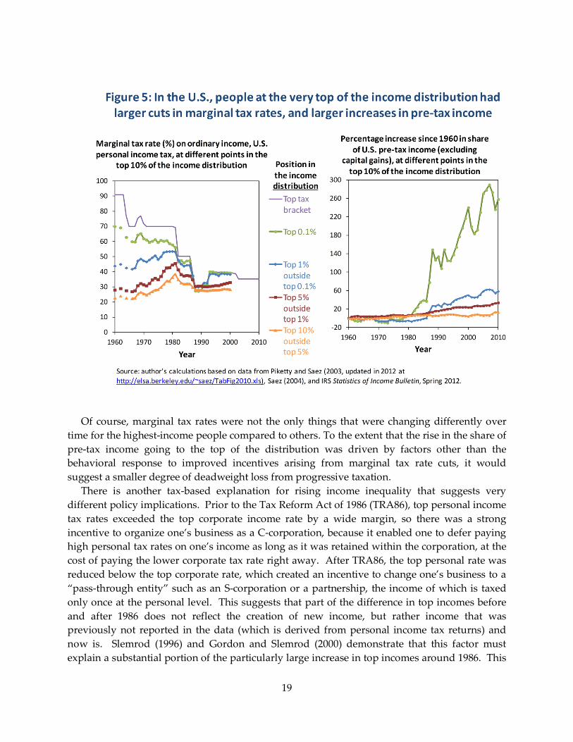
Of course, marginal tax rates were not the only things that were changing differently over

time for the highest-income people compared to others. To the extent that the rise in the share of pre-tax income going to the top of the distribution was driven by factors other than the behavioral response to improved incentives arising from marginal tax rate cuts, it would suggest a smaller degree of deadweight loss from progressive taxation.

There is another tax-based explanation for rising income inequality that suggests very different policy implications. Prior to the Tax Reform Act of 1986 (TRA86), top personal income tax rates exceeded the top corporate income rate by a wide margin, so there was a strong incentive to organize one’s business as a C-corporation, because it enabled one to defer paying high personal tax rates on one’s income as long as it was retained within the corporation, at the cost of paying the lower corporate tax rate right away. After TRA86, the top personal rate was reduced below the top corporate rate, which created an incentive to change one’s business to a “pass-through entity” such as an S-corporation or a partnership, the income of which is taxed only once at the personal level. This suggests that part of the difference in top incomes before and after 1986 does not reflect the creation of new income, but rather income that was previously not reported in the data (which is derived from personal income tax returns) and now is. Slemrod (1996) and Gordon and Slemrod (2000) demonstrate that this factor must explain a substantial portion of the particularly large increase in top incomes around 1986. This

19

cannot explain all of the rise in top income shares, as the share of pre-tax income going to the top of the income distribution still increases dramatically, just a bit less so, when we include pass-through entity income from our measure of income. But it is a contributing factor, which weakens the story about marginal tax cuts causing an increase in productive economic activity somewhat.

Another alternative explanation for rising income inequality emphasizes that it coincided with advancing globalization, as indicated for example by increasing shares of imports and exports in GDP. This may increase the demand for the labor of high-skill workers in the U.S., because they can now sell their skills to a wider market, and highly-skilled workers are scarcer in the rest of the world than in the U.S. Globalization may similarly depress wages for lower-skilled workers, because they now have to compete with abundant low-skill workers from the rest of the world (Stolper and Samuelson, 1941; Krugman 2008). A second hypothesis is skill-biased technical change (Katz and Murphy, 1992; Bound and Johnson, 2002; Card and DiNardo, 2002; Garicano and Rossi-Hansberg 2006; Garicano and Hubbard 2007). Technology has arguably changed over time in ways that complement the skills of highly-skilled workers, and substitute for the skills of low-skilled workers. A third hypothesis, closely related to the previous two, is the “superstar” theory suggested by Sherwin Rosen (1981). In this theory, compensation for the very best performers in each field rises over time relative to compensation for others, because both globalization and technology are enabling the best to sell their skills to a wider and wider market over time, which displaces demand for those who are less-than-the best. This is easiest to see for entertainers, but could easily apply to other professions as well.

Another hypothesis is that the increasing inequality may be explained to some extent by executive compensation practices (Bebchuk and Walker, 2002; Bebchuk and Grinstein, 2005; Eissa and Giertz, 2009; Friedman and Saks, 2010; Gabaix and Landier, 2008; Gordon and Dew-Becker, 2008; Kaplan and Rauh 2010; Murphy 2002; Piketty and Saez 2006). A large share of executive pay comes in the form of stock options, and almost all stock options are treated as wage and salary compensation on tax returns when they are exercised (Goolsbee 2000).11 Because of this, the values of stock options exercised by employees are generally counted in the measures of income used in the income inequality literature. It is clear that executive compensation has increased greatly over time, but there is a raging debate over why this has happened, and whether there are enough executives for this to explain much of the rise in top income shares. Bebchuk and Walker (2002) and Bebchuk and Grinstein (2005), among others, have argued that high and rising executive pay reflect the fact that the pay of executives is set by their peers on the board of directors, that free rider problems prevent shareholders from doing sufficient monitoring of executive compensation practices, and that the problems have

11 Federal income tax law classifies compensation in the form of stock options into two categories. “Non-qualified” stock options are treated as wage and salary income when exercised. “Incentive” stock options are taxed as capital gains at the personal level when exercised, but are denied a deduction for labor compensation from the corporate income tax. Under current law, the non-qualified options are generally much preferable from a tax standpoint compared to incentive stock options and Goolsbee (2000) indicates that almost all stock options used in executive compensation are of the non-qualified type. However, before 1986 incentive stock options were less tax disadvantaged.

20

been getting worse over time. Bertrand and Mullainathan (2001) argue that optimal executive compensation practices would reward executives for their own efforts but not for luck. So for example, executives would optimally be rewarded for an increase in their firm’s share price relative to the share prices of other firms in the economy, but would not be rewarded for increases in the firm’s share price that are driven by an overall increase in economy-wide equity prices (for example due to bubble psychology or a reduction in the risk premium demanded by investors). They present empirical evidence indicating that executive pay is in fact equally influenced by effort and luck, and that luck has less of influence on executive pay in firms that various observable indicators suggest are better governed. This supports the notion that executive compensation practices are not entirely efficient. Many others (for example, Murphy 2002) argue that executive pay reflects economically efficient compensation necessary to align executive incentives with those of shareholders. Gabaix and Landier (2008) argue that the increasing scale of firms has been critical to explaining rising executive pay; however, Friedman and Saks (2010) show that real executive pay grew very little between World War II and the mid-1970s despite large increases in firm size during that period, casting doubt on the Gabaix and Landier hypothesis.

Kaplan (2012) points to data in Bakija, Cole, and Heim (2012) which shows that between 1979 and 2005, a growing share of income earned by executives in the top 0.1 percent of the income distribution went to executives of pass-through entities (such as S-corporations, partnerships, and sole proprietorships), as opposed to executives who earned most of their income as salary. Kaplan interprets this as evidence against the kinds of abusive executive compensation problems described above, since presumably executives who earn most of their income from salary are more likely to be executives of publicly traded corporations with large numbers of shareholders, whereas pass-through entities typically have a smaller number of owners, so we would expect abusive executive compensation practices to be a smaller problem there. If abusive executive compensation practices were an important part of the explanation for rising inequality, goes the argument, we would have expected to see incomes grow faster over time for executives of firms that are more likely to be publicly traded, and this fact seems to suggest that the opposite happened. when of firms that are more likely to have larger numbers of shareholders grow faster. Mankiw (2013, p. 31) cites this evidence in his article “Defending the One Percent.” However, this is not a convincing piece of evidence about executive compensation practices at all, because there is a clear alternative explanation for why executives of pass-through entities accounted for a growing share of income over time. As noted above, when the Tax Reform Act (TRA86) of 1986 pushed top personal income tax rates down below the corporate tax rate, it greatly increased the tax advantages of organizing one’s business as a pass-through entity rather than as a C-corporation, and large numbers of C-corporations switched to pass-through entity status as a result.

Yet another hypothesis is that technological change and compensation practices in financial professions play a critical role. Philippon and Reshef (2009) show that the skill-intensity of financial sector jobs has grown dramatically since the early 1980s. Moreover, they estimate that since the mid-1990s, financial sector workers have been capturing rents that account for between 30 and 50 percent of the difference between financial sector wages and wages in other jobs. Of course, compensation of executives, financial professionals, and perhaps top earners in

21

other fields (such as high technology) can be expected to be heavily influenced by financial market asset prices, particularly stock prices, which went up dramatically at the same time as the increase in inequality. So part of the rising inequality may simply reflect that people in these professions have compensation that is strongly tied to the stock market, and got lucky when the stock market went way up. This might be counted as a separate hypothesis or a subset of the previous two.

Another hypothesis related to the past few is that social norms and institutions in the United States may be changing over time in a way that reduces opposition to high pay (see, e.g., Piketty and Saez 2006). For example, perhaps the “outrage constraint” once played an important role in preventing executives and their peers on the board from colluding to grant excessively high pay, but social norms against high pay have weakened over time so this constraint no longer binds. Alternatively, perhaps the social norms of old were harming efficiency by preventing corporate boards from granting stock options that were sufficiently large to align the incentives of the executive with those of the shareholders.

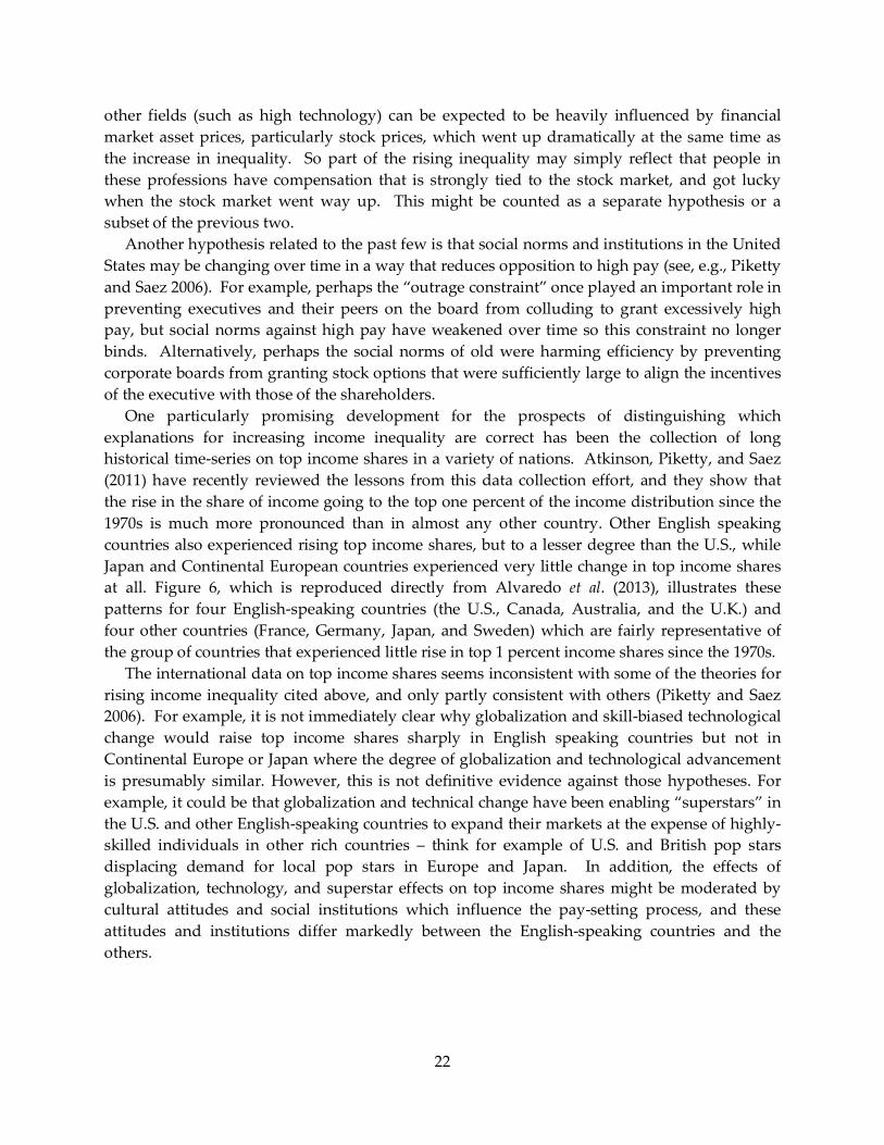
One particularly promising development for the prospects of distinguishing which explanations for increasing income inequality are correct has been the collection of long historical time-series on top income shares in a variety of nations. Atkinson, Piketty, and Saez (2011) have recently reviewed the lessons from this data collection effort, and they show that the rise in the share of income going to the top one percent of the income distribution since the 1970s is much more pronounced than in almost any other country. Other English speaking countries also experienced rising top income shares, but to a lesser degree than the U.S., while Japan and Continental European countries experienced very little change in top income shares at all. Figure 6, which is reproduced directly from Alvaredo et al. (2013), illustrates these patterns for four English-speaking countries (the U.S., Canada, Australia, and the U.K.) and four other countries (France, Germany, Japan, and Sweden) which are fairly representative of the group of countries that experienced little rise in top 1 percent income shares since the 1970s.

The international data on top income shares seems inconsistent with some of the theories for rising income inequality cited above, and only partly consistent with others (Piketty and Saez 2006). For example, it is not immediately clear why globalization and skill-biased technological change would raise top income shares sharply in English speaking countries but not in Continental Europe or Japan where the degree of globalization and technological advancement is presumably similar. However, this is not definitive evidence against those hypotheses. For example, it could be that globalization and technical change have been enabling “superstars” in the U.S. and other English-speaking countries to expand their markets at the expense of highly-skilled individuals in other rich countries – think for example of U.S. and British pop stars displacing demand for local pop stars in Europe and Japan. In addition, the effects of globalization, technology, and superstar effects on top income shares might be moderated by cultural attitudes and social institutions which influence the pay-setting process, and these attitudes and institutions differ markedly between the English-speaking countries and the others.

22

Figure 6

Source: reproduced directly from Alvaredo et al. (2013).

23

Initial efforts to use cross-country data to econometrically estimate the relationship between marginal tax rates and top income shares do find a correlation. Roine, Vlachos, and Waldenstrom (2008), estimate regressions using cross-country data from most of the 20th century, find that countries which experienced larger reductions in top marginal personal income tax rates had modestly larger increases in top income shares over time. A 10-percentage point reduction in the top marginal personal income tax rate is associated with a 0.4 percentage point increase in the percent of national income going to the top one percent of the income distribution.

Using data on 18 OECD countries from 1975 through 2008, Piketty, Saez, and Stantcheva (2011) find that countries that reduced top marginal personal income tax rates by larger amounts over time also experienced larger increases in the share of national income going to the top one percent of the income distribution, compared to countries that had smaller reductions in to marginal tax rates over time. Based on this relationship, they estimate that elasticity of income to the net-of-marginal-tax-rate share is 0.44 among income earners in the top one percent of the income distribution. If that represented a causal effect of improved incentives on productive economic behavior, it would imply that the revenue-maximizing marginal tax rate in the top bracket of the U.S. personal income tax would be about 60 percent, and the marginal deadweight loss per dollar of additional revenue raised from a top bracket taxpayer in the U.S. would be about $0.95. However, Piketty, Saez, and Stantcheva argue that in fact a large share of the response of reported top incomes to marginal tax rates represents rent-seeking – that is, top income earners are to some extent redistributing income from others to themselves rather than creating new income. As an example, they suggest that reduced top marginal income tax rates give executives an enhanced incentive to bargain in order to exploit market failures in the executive compensation pay-setting process of the sort discussed above, redistributing income from shareholders to themselves. Piketty, Saez, and Stantcheva show that there is no evidence across countries or in the U.S. time series of a correlation between top marginal tax rates and economic growth, and present this as evidence that some of the rise in top income shares may have represented rent-seeking as opposed to new productive income-earning efforts. They do acknowledge that this is at best circumstantial evidence, since so many other factors that they are not controlling for also affect economic growth. Based on this, they conclude that the elasticity of real productive income earning efforts to the net-of-tax-share is probably closer to 0.2, which would imply a revenue-maximizing top tax rate of 79 percent and a marginal deadweight loss per dollar of additional revenue collected from a top bracket taxpayer of $0.28. Diamond and Saez (2011) argue that incomes in the top percentile of the income distribution have gotten so high that the marginal utility of an additional dollar of income to these people must be very low compared to people lower down in the distribution, and argue on this basis that we ought to set tax rates on the highest earners close to the revenue-maximizing rate, which the evidence in Piketty, Saez and Stantcheva suggests would be significantly higher than the 39.6 percent tax rate prevailing in the U.S. today, but still considerably lower than the 91 percent top income tax rate that applied in the U.S. between World War II and the early 1960s.

Theories about executive compensation, financial market asset prices, social norms, and institutions could be important contributing factors to differences in the rate at which top income shares are rising in different countries, but estimating their influence is complicated by

24

the fact that we lack good observable indicators of social norms and executive compensation practices that are comparable across countries. Roine, Vlachos, and Waldenstrom’s analysis of cross-country panel data does finds that top income shares are strongly positively correlated with stock market capitalization. A corroborating piece of evidence for the role of executive compensation, pay-setting institutions, and stock market prices is that while Japan and the U.S. had similar changes in top marginal tax rates, in Japan it was illegal to compensate executives with stock options until 1997 (Bremner 1999), and stock prices in Japan crashed in the early 1990s and remained relatively flat thereafter. This might help explain the lack of rising top income shares in Japan. Executive stock options are legal in France, and stock prices rose even more in France than in the U.S. since the early 1980s; but average executive compensation in France is less than half of what it is in the U.S., which might be explained by social norms (The Economist, 2008, and Alcouffe and Alcouffe 2000). This could explain why top income shares seem largely unaffected by stock prices in France.

Bakija, Cole, and Heim (2012) provide evidence from tax return data on the occupations of people at the top of the income distribution in the U.S., and how the incomes of people in different highly-paid occupations have been changing over time, which is summarized in figures 7 and 8.

Figure 7 shows the share of pre-tax income going to the top 0.1 of the income distribution in the years between 1979 and 2005 when occupational data is available, and illustrates what share of that income was received by people in different occupations. In 2005, the top 0.1 percent of the income distribution accounted for 7.34 percent of all pre-tax income (excluding capital gains). Of that, 50 percent of the income was received by executives, managers, supervisors, or entrepreneurs of non-financial firms. Another 20 percent was received by financial executives and other financial professionals. Together, these occupations accounted for more than 70 percent of the increase in the share of pre-tax income going to the top 0.1 percent between 1979 and 2005.

25

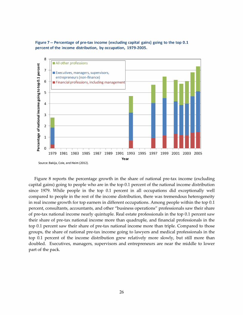
Figure 8 reports the percentage growth in the share of national pre-tax income (excluding

capital gains) going to people who are in the top 0.1 percent of the national income distribution since 1979. While people in the top 0.1 percent in all occupations did exceptionally well compared to people in the rest of the income distribution, there was tremendous heterogeneity in real income growth for top earners in different occupations. Among people within the top 0.1 percent, consultants, accountants, and other “business operations” professionals saw their share of pre-tax national income nearly quintuple. Real estate professionals in the top 0.1 percent saw their share of pre-tax national income more than quadruple, and financial professionals in the top 0.1 percent saw their share of pre-tax national income more than triple. Compared to those groups, the share of national pre-tax income going to lawyers and medical professionals in the top 0.1 percent of the income distribution grew relatively more slowly, but still more than doubled. Executives, managers, supervisors and entrepreneurs are near the middle to lower part of the pack.

26

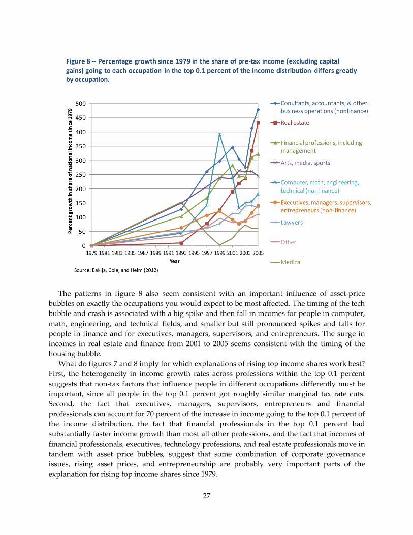
The patterns in figure 8 also seem consistent with an important influence of asset-price

bubbles on exactly the occupations you would expect to be most affected. The timing of the tech bubble and crash is associated with a big spike and then fall in incomes for people in computer, math, engineering, and technical fields, and smaller but still pronounced spikes and falls for people in finance and for executives, managers, supervisors, and entrepreneurs. The surge in incomes in real estate and finance from 2001 to 2005 seems consistent with the timing of the housing bubble.

What do figures 7 and 8 imply for which explanations of rising top income shares work best? First, the heterogeneity in income growth rates across professions within the top 0.1 percent suggests that non-tax factors that influence people in different occupations differently must be important, since all people in the top 0.1 percent got roughly similar marginal tax rate cuts. Second, the fact that executives, managers, supervisors, entrepreneurs and financial professionals can account for 70 percent of the increase in income going to the top 0.1 percent of the income distribution, the fact that financial professionals in the top 0.1 percent had substantially faster income growth than most all other professions, and the fact that incomes of financial professionals, executives, technology professions, and real estate professionals move in tandem with asset price bubbles, suggest that some combination of corporate governance issues, rising asset prices, and entrepreneurship are probably very important parts of the explanation for rising top income shares since 1979.

27

The fact that executives, managers, supervisors, and entrepreneurs account for such a large share of income at the top of the distribution may strengthen the case that abusive executive compensation practices could be important to explaining rising inequality. This is tempered by the fact that many of these people do not work for publicly traded firms, as evidenced for example by the fact that in recent years close to half of them earn the majority of their income from pass-through entities, which cannot be publicly traded, and by the fact that income growth of executives, managers, supervisors, and entrepreneurs was not unusually fast compared to that of people in other occupations in the top 0.1 percent. The large and growing share of executives, managers, and supervisors of pass-through entities in the top 0.1 percent of the income distribution also corroborates prior evidence suggesting that that shifting of income between the corporate and personal income tax bases is likely to be a particularly important part of the explanation for rising top income shares since 1979.

Relatively strong income growth in arts, media, and sports seems supportive of the “superstar” theory, although they only account for about 4 percent of pre-tax income received by the top 0.1 percent of the income distribution. The superstar phenomenon could apply broadly in many different types of occupations, though. For instance, technology and globalization now enable the best management consultants to sell their services to a much broader audience, and notably their occupational category (business operations) experienced the fastest income growth of all in the top 0.1 percent between 1979 and 2005. Malmendier and Tate (2009) present evidence on the phenomenon of “superstar CEOs.”

Clearly, there is still plenty of room for debate over how much each of the different factors considered above have contributed to the dramatic rise in top income shares in the U.S. in recent decades. The stakes in this debate are large, as different explanations for the rise in inequality can have very different implications for the economic efficiency costs of progressive tax-and-transfer policy, and different implications for the ethics of redistribution (for example because some explanations suggest luck played a larger role than effort).

28

References Alcouffe, Alain and Christiane Alcouffe. 2000. “Executive Compensation Setting Practices in France.” Long-Range Planning. Vol. 33, pp. 527-543. Alvaredo, Facundo, Anthony B. Atkinson, Thomas Piketty, and Emmanuel Saez. 2013. "The Top 1 Percent in International and Historical Perspective." Journal of Economic Perspectives. Vol. 27, no. 3, pp. 3-20. Atkinson, Anthony B., Thomas Piketty, and Emmanuel Saez. 2011. “Top Incomes in the Long Run of History.” Journal of Economic Literature. Vol. 49, No. 1, pp. 3-71. Autor, David H., Lawrence F. Katz, and Melissa S. Kearney. 2008. "Trends in U.S. Wage Inequality: Revising the Revisionists." Review of Economics and Statistics 90, no. 2: 300-323. Autor, David H., Frank Levy, and Richard J. Murnane. 2003. "The Skill Content of Recent Technological Change: An Empirical Exploration." Quarterly Journal of Economics 118, no. 4: 1279-1333. Bakija, Jon. 2011. “Notes on Indifference Curve Analysis of the Choice between Leisure and Labor, and the Deadweight Loss of Taxation.” <http://web.williams.edu/Economics/bakija/Bakija-Notes-on-Indifference-Curve-Analysis-of-the-Choice-Between-Leisure-and-Labor.pdf > Bakija, Jon, Adam Cole, and Brad Heim. 2012. “Jobs and Income Growth of Top Earners and the Causes of Changing Income Inequality: Evidence from U.S. Tax Return Data” Working Paper, Williams College (http://web.williams.edu/Economics/wp/BakijaColeHeimJobsIncomeGrowthTopEarners.pdf). Bebchuk, Lucian, Jesse M. Fried and David I. Walker. 2002. “Managerial Power and Rent Extraction in the Design of Executive Compensation.” The University of Chicago Law Review 69, No. 3: 751-846.

Bebchuk, Lucian, and Yaniv Grinstein. "The Growth of Executive Pay." Oxford Review of Economic Policy 21, no. 2 (Summer 2005): 283-303.

Bertrand, Marianne, and Sendhil Mullainathan. 2001. "Are CEOs Rewarded for Luck? The Ones without Principles Are." Quarterly Journal of Economics. Vol. 116, no. 3: 901-932.

Boadway, Robin. 2010. "Efficiency and Redistribution: An Evaluative Review of Louis Kaplow's The Theory of Taxation and Public Economics." Journal of Economic Literature Vol. 48, no. 4: 964-979

29

Bound, J., and G. Johnson. 1992. ‘‘Changes in the Structure of Wages in the 1980s: An Evaluation of Alternative Explanations,’’ American Economic Review. 82 (June), 371–392.

Bremner, Brian. 1999. “The Stock-Option Option Comes to Japan.” Businessweek Online. April 19. Card, David, and John E. DiNardo. 2002. "Skill-Biased Technological Change and Rising Wage Inequality: Some Problems and Puzzles." Journal of Labor Economics 20, no. 4: 733-783.

Congressional Budget Office. 2012a The Distribution of Household Income and Federal Taxes, 2008 and 2009. Washington, DC, July 10. <http://www.cbo.gov/sites/default/files/cbofiles/attachments/43373-06-11-HouseholdIncomeandFedTaxes.pdf> (accessed July 14, 2012). Congressional Budget Office. 2012b The Distribution of Household Income and Federal Taxes, 2008 and 2009: Supplemental Data. Washington, DC, July 10. <http://www.cbo.gov/sites/default/files/cbofiles/attachments/43373-Supplemental_Tables_Final.xls> (accessed July 14, 2012). Diamond, Peter and Emmanuel Saez. 2011. “"The Case for a Progressive Tax: From Basic Research to Policy Recommendations." Journal of Economic Perspectives. Vol. 5, No. 4 (Fall), pp. 165-190 <http://www.aeaweb.org/atypon.php?return_to=/doi/pdfplus/10.1257/jep.25.4.165>. Dworkin, Ronald. 2000. Sovereign Virtue: The Theory and Practice of Equality. Cambridge, MA: Harvard University Press. The Economist. 2008. “Executive Pay in Europe: Pay Attention.” June 12.

Eissa, Nada O. and Seth H. Giertz. 2009. “Trends in High Incomes and Behavioral Responses to Taxation: Evidence from Executive Compensation and Statistics of Income.” Working Paper.

Friedman, David. 1997. Hidden Order: The Economics of Everyday Life. New York: HarperBusiness. Frydman, Carola and Raven E. Saks. 2010. “Executive Compensation: A New View from a Long-Term Perspective, 1936-2005.” Review of Financial Studies, Vol. 23 No. 5, pp. 2099-2138.

Gabaix, Xavier, and Augustin Landier. 2008. "Why Has CEO Pay Increased So Much?" Quarterly Journal of Economics 123, no. 1: 49-100. Garicano, L., and E. Rossi-Hansberg. 2006. “Organization and Inequality in a Knowledge Economy.” Quarterly Journal of Economics. 121:1383–435

30

Garicano, L., and T. Hubbard. 2007. “The Returns to Knowledge Hierarchies.” NBER Working Paper No. 12815 (January).

Gordon, Robert J. and Ian Dew-Becker. 2008. “Controversies About the Rise of American Inequality: A Survey.” NBER Working Paper No. 13982.

Gordon, Roger and Joel Slemrod. 2000. “Are `Real' Responses to Taxes Simply Income Shifting Between Corporate and Personal Tax Bases?" In Joel Slemrod, ed., Does Atlas Shrug? The Economic Consequences of Taxing the Rich, Cambridge University Press.

Gruber, Jonathan. 2011. Public Finance and Public Policy, New York: Worth Publishers. Kaiser Commission on Medicaid and the Uninsured. 2010. The Medicaid Program at a Glance. June. <http://www.kff.org/medicaid/upload/7235-04.pdf> (accessed August 20, 2012). Kaiser Commission on Medicaid and the Uninsured. 2012a. 5 Key Questions and Answers About Medicaid: Chartpack. May. <http://www.kff.org/medicaid/upload/8162-02.pdf> (accessed August 20, 2012). Kaiser Commission on Medicaid and the Uninsured. 2012b. Health Coverage of Children: The Role of Medicaid and CHIP. July. <http://www.kff.org/uninsured/upload/7698-06.pdf> (accessed August 20, 2012). Kaplan, Steven N. 2012. “Executive Compensation and Corporate Governance in the U.S.: Perceptions, Facts, and Challenges.” NBER Working Paper 18395. Kaplan, Steven N. and Joshua Rauh. 2010. “Wall Street and Main Street: What Contributes to the Rise in High Incomes?” Review of Financial Studies, Vol. 23, No. 3., pp. 1004-1050.

Kaplow, Louis. 2008. The Theory of Taxation and Public Economics, Princeton and Oxford: Princeton University Press. Katz, Lawrence and Kevin Murphy. 1992. “Changes in RelativeWages, 1963–1987: Supply and Demand Factors.” Quarterly Journal of Economics 107:35–78.

Koll, Douglas K. 2003. “Shareholder Oppression & Dividend Policy in the Close Corporation.” Washington & Lee Law Review, Vol. 60, pp. 841-924.

Krugman, Paul R. 2008. "Trade and Wages, Reconsidered." Brookings Papers on Economic Activity , no. 2: 103-138.

31

Levy, Frank, and Richard J. Murnane. 1992. "U.S. Earnings Levels and Earnings Inequality: A Review of Recent Trends and Proposed Explanations." Journal of Economic Literature 30, no. 3: 1333-1381. Malmendier, Ulrike, and Geoffrey Tate. 2009. “Superstar CEOs.” Quarterly Journal of Economics. (November) pp. 1593-1638.

Mankiw, N. Gregory. 2010. "Spreading the Wealth Around: Reflections Inspired by Joe the Plumber: Presidential Address." Eastern Economic Journal. Vol. 36, No. 3, pp. 285-298. Mankiw, N. Gregory. 2013. “Defending the One Percent.” Journal of Economic Perspectives. Summer, pp. 21-34. Mankiw, Gregory and Matthew Weinzierl. 2010. “The Optimal Taxation of Height: A Case Study of Utilitarian Income Redistribution." American Economic Journal: Economic Policy, Vol. 2, No. 1, pp. 155-76. Mankiw, N. Gregory, Matthew Weinzierl, and Danny Yagan. 2009. "Optimal Taxation in Theory and Practice." Journal of Economic Perspectives, Vol. 23, no. 4: 147-174. <http://www.aeaweb.org/atypon.php?return_to=/doi/pdfplus/10.1257/jep.23.4.147>. Mirrlees, James A. 1971. "An Exploration in the Theory of Optimal Income Taxation." Review of Economic Studies, Vol. 38, pp. 175-208. Murphy, Kevin J. 2002. “Explaining Executive Compensation: Managerial Power versus the Perceived Cost of Stock Options.” The University of Chicago Law Review 69, No. 3: 847-869.

Musgrave, Richard A. 1990. “Horizontal Equity, Once More.” National Tax Journal. Vol. 43, No. 2, pp. 113-22. <http://ntj.tax.org/wwtax/ntjrec.nsf/A42168FEAB9541FF8525686C00686DCA/$FILE/v43n2113.pdf>. Okun, Arthur. 1975. Equality and Efficiency: The Big Tradeoff. Washington: Brookings Institution Press. Philippon, Thomas and Ariell Reshef. 2009. “Wages and Human Capital in the U.S. Financial Industry: 1909-2006.” NBER Working Paper No. 14644.

Piketty, Thomas, and Emmanuel Saez. 2003. “Income Inequality in the United States, 1913–1998.” Quarterly Journal of Economics 118, no. 1 (February): 1–39. (Tables and figures updated through 2011 in January 2013 at <http://elsa.berkeley.edu/~saez/TabFig2011prel.xls>, accessed June 28, 2013).

32

Piketty, Thomas, and Emmanuel Saez. 2006. "The Evolution of Top Incomes: A Historical and International Perspective." American Economic Review 96, no. 2: 200-205.

Piketty, Thomas, Emanuel Saez, and Irina Stantcheva. 2011. “Optimal Taxation of Top Labor Incomes: A Tale of Three Elasticities.” NBER Working Paper No. 17616. (Link to freely available working paper version: http://elsa.berkeley.edu/~saez/piketty-saez-stantchevaNBER11thirdelasticity.pdf) Rawls, John. 1971. A Theory of Justice. Cambridge, MA: Harvard University Press. Roemer, John E. 1998. Equality of Opportunity. Harvard University Press. Roine, Jesper, Jonas Vlachos, and Daniel Waldenstrom. 2009. "The Long-Run Determinants of Inequality: What Can We Learn from Top Income Data?" Journal of Public Economics 93, no. 7-8: 974-988. Rosen, Harvey S., and Ted Gayer. 2008. Public Finance, 8th ed. New York: McGraw-Hill Irwin. Rosen, Sherwin. 1981. "The Economics of Superstars." American Economic Review Vol. 71, no. 5: 845-858.

Saez, Emmanuel. 2004. “Reported Incomes and Marginal Tax Rates, 1960–2000: Evidence and Policy Implications.” In Tax Policy and the Economy, Volume 18, edited by James M. Poterba, 117–74. Cambridge and London: MIT Press. (http://elsa.berkeley.edu/~saez/saezTPE04.pdf) Saez, Emmanuel, Joel Slemrod, and Seth Giertz. 2012. “The Elasticity of Taxable Income with Respect to Marginal Tax Rates: A Critical Review.” Journal of Economic Literature. Vol. 50, No. 1, pp. 3-50. (Link to freely available working paper version: http://elsa.berkeley.edu/~saez/saez-slemrod-giertzJEL12.pdf) Slemrod, Joel, and Jon Bakija. Forthcoming. Taxing Ourselves: a Citizen’s Guide to the Debate over Taxes. 5th edition. MIT Press. Stolper, Wolfgang, and Paul Samuelson. 1941. “Protection and Real Wages.” Review of Economic Studies 9, no. 1: 58–73.

Urban-Brookings Tax Policy Center. 2013a. “Table T13-0040 -- Baseline Distribution of Cash Income and Federal Taxes by Filing Status; by Cash Income Percentile, 2013” Jan. 17. <http://www.taxpolicycenter.org/numbers/Content/Excel/T13-0040.xls> (accessed June 17, 2013). Urban-Brookings Tax Policy Center. 2013b. “Table T13-0045 -- Baseline Average Effective Federal Tax Rates by Filing Status; by Cash Income Percentile, 2013.” Jan. 17. <http://www.taxpolicycenter.org/numbers/Content/Excel/T13-0045.xls> (accessed June 17, 2013).

33

Urban-Brookings Tax Policy Center. 2013c. “Table T13-0049 -- Baseline Share of Federal Taxes by Filing Status; by Cash Income Percentile, 2013.” Jan. 17. Weisbach, David. 2003. “Should Legal Rules be used to Redistribute Income?” University of Chicago Law Review. Vol. 70.

34