socioeconomic distribution of emissions and resource use in ireland

at SciVerse ScienceDirect

Journal of Environmental Management 112 (2012) 186e198

Contents lists available

Journal of Environmental Management

journal homepage: www.elsevier .com/locate/ jenvman

Socioeconomic distribution of emissions and resource use in Ireland

Sean Lyons a,b,*, Anne Pentecost a, Richard S.J. Tol a,b,c,d

a Economic and Social Research Institute, Dublin, IrelandbDepartment of Economics, Trinity College Dublin, Dublin, Irelandc Institute for Environmental Studies, Vrije Universiteit, Amsterdam, The NetherlandsdDepartment for Spatial Economics, Vrije Universiteit, Amsterdam, The Netherlands

a r t i c l e i n f o

Article history:Received 21 March 2012Received in revised form16 July 2012Accepted 21 July 2012Available online

Keywords:PollutionHousehold emissionsDistributional analysis

JEL classifications:Q52Q53D39D57

* Corresponding author. Economic and Social RSquare, Sir John Rogerson’s Quay, Dublin 2, Irelanfax: þ353 1 863 2100.

E-mail address: [email protected] (S. Lyons).

0301-4797/$ e see front matter � 2012 Elsevier Ltd.http://dx.doi.org/10.1016/j.jenvman.2012.07.019

a b s t r a c t

This paper aims to determine emissions polluted directly and indirectly by an average person, for eachhousehold type, across a wide range of emissions. There are five household type categories: location,income decile, household composition, size and number of disabled residents. Ireland’s SustainableDevelopment Model (ISus) is used which allows the analysis of direct and indirect sources of pollutionper household as the model is based on an inputeoutput methodology. Four sets of results are presented:first for greenhouse gas emissions, second for air pollutants, third for persistent organic pollutants andlastly for metals. An analysis section shows how the picture changes when one controls for the size andincome of households. All results analysed are for the year 2006. Most greenhouse gas and metalemissions are polluted via indirect means, although direct sources of emissions play a role for CO2, SO2

and CO. The results suggest that the richest decile is the biggest emitter and poorer and larger house-holds are seen to emit the least per person. It is also shown that household income has a strongerrelationship with pollution than household size per person.

� 2012 Elsevier Ltd. All rights reserved.

1. Introduction

Households differ, both in idiosyncratic ways and in the form ofsystematic differences between household types. One effect ofthese variations is that different household types exert differentpressures on the environment through their varying behaviour. Forexample, people in rural areas tend to use their cars more often andpeople who are out of work have a reason to heat their home in theday time. It is important to be able to quantify these distributionaldifferences as they may have implications for environmental policymaking (Lee and Tansel, 2012). For example, energy is a necessarygood and thus policies that increase the cost of energy tend to beregressive; that is, poorer households spend proportionately moreof their income on household energy than richer households.Additional policies may therefore be needed to offset the equityimpact of regressive environmental policies. This paper attempts to

esearch Institute, Whitakerd. Tel.: þ353 1 863 2019;

All rights reserved.

assess whether different household characteristics matter for theamount of pollution emitted by the residential sector; for exampledo richer households emit more than poorer households, urbanhouseholds emit more than rural or do households with childrenpollute more than those without? Although this paper does notdraw formal policy conclusions, it does show that there aredifferences in household emissions due to different householdcharacteristics and this should be borne in mind by policymakers.The paper thus adds to the environmental justice literature (e.g.,Krieg and Faber, 2004), which has primarily focussed on the USA.

This paper is part of a broader literature on distributionalanalysis at the household level. Stokes et al. (1994) use a surveyanalysis for Melbourne (Australia) asking residents about theirunderstanding of the greenhouse gas effect and their contributionsto reducing the amount of carbon dioxide emitted. The author’sanalysis focuses on whether the understanding of climate changeissues has resulted in fewer CO2 emissions from four differenthousehold types: location, composition, size and economicresources. This paper expands on the household distributionalanalysis of Stokes et al. (1994) twofold; firstly by including incomedeciles and the number of disabled residents in household typesand secondly by analysing the distribution of household pollution

Delta:1_given name

Delta:1_surname

Delta:1_given name

mailto:[email protected]

www.sciencedirect.com/science/journal/03014797

http://www.elsevier.com/locate/jenvman

http://dx.doi.org/10.1016/j.jenvman.2012.07.019



Table 1The 20 final demand sectors used (NACE19 plus the residential sector).

Agriculture, fishery and forestry Rubber and plastic production

Coal, peat, petroleum, metal oresand quarrying

Residential

Food, beverage and tobacco TransportTextiles, clothing, leather and footwear Services excluding transportWood and wood products ConstructionPulp, paper and print production Fuel, power and waterChemical production Other manufacturingNon-metallic mineral production Transport equipmentMetal production excluding machinery

and transport equipmentElectrical goods

Agriculture and industry machinery Office and data processingmachines

S. Lyons et al. / Journal of Environmental Management 112 (2012) 186e198 187

for forty-three1 emissions. Our study also differs given its focus onIreland for the year 2006.

Most distributional analysis undertaken in the literatureestimates the effects of a carbon tax on different types ofhouseholds and studies have been done for several countriesincluding Ireland (Verde and Tol, 2009), Spain (Labandeira andLabeaga, 1999), the USA (Hassett et al., 2007) and the UK(Symons et al., 1994). All papers find that a carbon tax isregressive, indeed Hassett et al. (2007) find that the lowestincome burden can be up to four times that of the richest decile.When Hassett et al. (2007) use consumption as a proxy forincome, however, the authors find that a carbon tax is lessregressive. The introduction of a carbon tax in the UK and Irelandis also found to be highly regressive, however less so for Spain.The studies use an inputeoutput methodology which not onlyallows the study of the whole economy rather than just onespecific sector but also it highlights the significance of indirectemissions from final consumption (Labandeira and Labeaga,1999) and thus a decomposition of the importance of directand indirect emission sources for each household type.

This paper aims to determine direct and indirect emissions foran average person by household type, across a wide range ofemissions. Direct emissions are those generated when a house-hold pollutes from personal consumption and over which it hasdirect control, such as petrol use from driving a car or fuelsburned for home heating. Indirect emissions are emitted duringproduction processes over which a household does not havedirect control; for example pollution from power stations used toprovide energy to households. The household type categories weuse are location (urban and rural), income decile, household size,household composition and number of disabled residents. To dothis Ireland’s Sustainable Development Model (ISus) is usedwhich allows the analysis of direct and indirect sources ofpollution per household. Four sets of results are presented: firstfor greenhouse gas emissions, second for air pollutants, third forpersistent organic pollutants and lastly for metals. An analysissection shows how the picture changes when one controls forthe size and income of households. All results analysed are forthe year 2006.

The main conclusions are that indirect emission sources arethe main contributor of pollution for most emissions; directemissions play different roles for each emission, and income isa more important factor than household size for the quantities ofpollution emitted. The paper is set up as follows; Section 2presents the methodology, Section 3 describes the data, Section4 analyses the results,2 Section 5 offers some analysis and Section6 concludes.

2. Methodology

The first step is to run an inputeoutput model to determineemissions from production attributed to twenty final demandsectors (shown in Table 1). The ISus model uses the inputeoutputtable for 2000 (CSO, 2006) updated to 2006 using the RASmethod (Parikh, 1979). The standard inputeoutput model is set-upas (1) where X is a vector of production, Y is a vector of finaldemand, A is a matrix of production coefficients, I is the identitymatrix and L is the Leontief inverse.

1 Given the large number of emissions only the most important are analysed inthis paper. The remaining household emission distribution results are available onrequest.

2 Results for HFC’s, ammonia and nitrogen oxide can be found in the Appendixdue to the large number of emissions in the model.

X ¼ AX þ Y5ðI � AÞX ¼ Y5X ¼ ðI � AÞ�1Y ¼ LY (1)

Let R denote emissions and B the matrix of emission intensitiesof production. Then

R ¼ BX ¼ BLY (2)

As a next step, we split final demand Y into its components,those being households, charities, government, investment,inventories and exports:

R ¼ BLY ¼ BLðE þ C þ Gþ K þ I þ XÞ (3)

Finally, household expenditure E is split into the expenditure byhousehold type:

R ¼ BL

Xt

Et þ C þ Gþ K þ I þ X

!(4)

The indirect emissions from household type t are thus defined as

Rt ¼ BLEt (5)

The distribution of direct emissions by type of household3 areestimated for pollutants produced by fuel use. They are calculatedby using the data on the quantity of household fuel used from theCSO anonymised Household Budget Survey data file (CSO, 2007).For each household type, the emission shares add to unity. Forexample, for CO2 from fossil fuels the share emitted per person inan urban household is 0.585 and the share for a rural household is0.415. These figures are calculated by using the emissions factordatabase (EFDB) which converts the fuel use data into commonunits. Fuel use is thenmultiplied by the appropriate emission factorfrom the EFDB to find each individual household’s (of the 6884 inthe survey) contribution to total emissions. These households arethen aggregated by household type and total emissions for eachtype is then multiplied by a population grossing factor which yieldsthe national share of each emission produced by each householdcategory for each emission. Direct emissions are found by multi-plying the residential total emissions for each pollutant by thehousehold-type share for each pollutant. Household types areaggregated and compared against each other, for example urbanversus rural households, richer against poorer households andalternative household compositions (single, with or without chil-dren for example). Hypotheses relating to household type that we

3 Household type categories being: location (urban or rural), income decile (1,poorest to richest, 10), household size (1 person to 7 þ people), householdcomposition (single adults working and retired, a couple, a couple with 1, 2 3 or4 þ children and a single parent) and number of disabled residents (none to 3 ormore).

S. Lyons et al. / Journal of Environmental Management 112 (2012) 186e198188

attempt to analyse are given in Table 2 below. In addition, this paperalso examines whether households pollute more through direct orindirect channels. This could potentially be an important issue ashouseholds would be able to curb emissions from direct sourcesmore easily, if a tax was introduced for example, than those viaindirect means.

Table 3Variable descriptions.

Variable Description (years available, source, measurement unit)

CO2 from fossil fuel Carbon dioxide emissions from fossil fuels 1990e2009,(Duffy et al., 2011) thousand tonnes

CO2 other Carbon dioxide emissions from non fossil fuels1990e2009 (Duffy et al., 2011) thousand tonnes

CH4 Methane emissions 1990e2009 (Duffy et al., 2011)thousand tonnes

N2O Nitrous oxide emissions 1990e2009 (Duffy et al., 2011)thousand tonnes

HFC23 Halofluorocarbon emissions 1990e2095(Duffy et al., 2011) tonnes of CO2 equivalentHFC32

HFC134aHFC125HFC143aHFC152aHFC227eaCF4 Perfluorocarbon emissions 1990e2009

(Duffy et al., 2011) tonnes of CO2 equivalentC2F6C4F8SF6 Sulphurhexafluoride emissions 1990e2009

3. Data employed

The ISus model is based on both environmental and economicdata and for this study, emissions are broken down into direct andindirect emissions. The source used for information on directemissions is the anonymised data file for the Irish HouseholdBudget Survey (HBS) which is a random sample of representativehouseholds in Ireland. The main aim of this survey is to quantifyhow much the average household (by household type) spends oneach basket of goods (milk and boys clothes, for example) for theweighting of the CPI index and is carried out by the CentralStatistics Office (CSO, 2007). In the most recent 2004/2005 survey6884 private households in Ireland participated (a 47% responserate). In this cross-sectional micro dataset detailed information isalso provided on income and household facilities, for example it ispossible to examine which household characteristics, whichappliances and which heating and cooking methods significantlyinfluence the amount of energy used in the home. In addition,households are asked to report expenditure on, as well as quantityused, of different fuel types in the past year.

Table 2Hypotheses to be examined.

Household type Hypothesis / research question

Location Do rural households emit more than urban ones?Rural households may use private transport moreoften and have longer journeys leading to higheremissions. Urban areas tend to be far busier thanrural areas and thus usage of constant publictransport, for example, may induce urban householdsto have higher pollution levels. The split betweendirect and indirect emissions may play a large partrelative to location where rural households arehypothesised to pollute more directly but urbanhouseholds are hypothesised to have higherindirect emissions.

Income decile Do richer households emit more than poorer ones?Richer households would be able to afford a higherenergy use than poorer households leading to higheremissions. Poorer households however may not beable to afford ‘greener technology’ such as extrainsulation or more efficient heating systems thusleading to higher emissions.

Household size Do larger households emit more than smaller ones?If economies of scale in consumption are present thenhouseholds with more people in would, per capita,emit less than those with fewer residents. With moreresidents usage is higher however, which may leadto higher emissions for a larger household.

Household composition How does household composition affect emissions?Do those with children emit less (per head)if economies of scale in consumption are present?Retired households may emit more than a workinghousehold as they are potentially at home moreduring the day. A single parent may not be able toafford as much energy consumption as a householdwhere two working adults reside leading to fewerhousehold emissions.

Number of disabledresidents

Does the number of disabled residents matter forhousehold emissions? For example, emissions maydiffer due to the share of time spent in the home,requirements for extra heating or specialisedelectrical equipment.

The emissions data are taken from a range of sources found inTable 3 along with variable descriptions. The EnvironmentalProtection Agency (EPA) data sources for the air emissions in thispaper have been used previously for Ireland by Ferreira and Moro(2011); however, with a focus on environmental accountingrather than distributional analysis.

(Duffy et al., 2011) tonnes CO2 equivalentSO2 Sulphur dioxide emissions 1990e2009

(Duffy et al., 2011) thousand tonnesNOx Oxides of nitrogen 1990e2009 (Duffy et al., 2011)

thousand tonnesCO Carbon monoxide 1990e2009 (Duffy et al., 2011)

thousand tonnesNMVOC Non-methane volatile organic compounds 1990e2005

(Duffy et al., 2011) thousand tonnesNH3 Ammonia 1990e2009 (CSO Environmental Accounts,

2010) thousand tonnesBOD Organic water pollution emissions 1990e2009 (Scott,

1999) thousand tonnesDioxin (water) Dioxin emissions to water 1990e2009

(Hayes and Murnane, 2002) g TECDioxin (air) Dioxin emissions to air 1990e2009

(Hayes and Murnane, 2002) g TECDioxin(land) Dioxin emissions to land 1990e2009

(Hayes and Murnane, 2002) g TECPCB (air) Polychlorinated biphenyl emissions to air 1990e2009

(Creedon et al., 2010) kgPCB (land) Polychlorinated biphenyl emissions to land 1990e2009

(Creedon et al., 2010) kgHCB (air) Hexachlorobenzene emissions to air 1990e2009

(Creedon et al., 2010) kgHCB (land) Hexachlorobenzene emissions to land 1990e2009

(Creedon et al., 2010) kgHCB (water) Hexachlorobenzene emissions to water 1990e2009

(Creedon et al., 2010) kgBenzo(a)pyrene Emissions 1990e2009 (Creedon et al., 2010) kgBenzo(b)fluoranthene Emissions 1990e2009 (Creedon et al., 2010) kgBenzo(k)fluoranthene Emissions 1990e2009 (Creedon et al., 2010) kgIndeno(1,2,3)pyrene Emissions 1990e2009 (Creedon et al., 2010) kgMercury Emissions 2001e2009 (Integrated Pollution Prevention

Control (IPPC)) kgCadmium Emissions 1996e2009 (IPPC, 2011) kgLead Emissions 1996e2009 (IPPC, 2011) kgChromium Emissions 1996e2009 (IPPC, 2011) kgArsenic Emissions 1996e2009 (IPPC, 2011) kgZinc Emissions 1996e2009 (IPPC, 2011) kgCopper Emissions 1996e2009 (IPPC, 2011) kgNickel Emissions 1996e2009 (IPPC, 2011) kgPopulation 1990e2009 (ESRI’s databank) thousands of peopleOutput 1990e2009 (ESRI’s databank) million euro constant

2004 gross output

0% 10% 20% 30% 40% 50% 60% 70% 80% 90% 100%

Benzo(a)pyreneIndeno(1,2,3)pyrene

PCB (air)Dioxin (air)

Benzo(b)fluorantheneDioxin (land)

Benzo(k)fluorantheneCO

SO2CO2 (fossil)

NMVOCNOx

Dioxin (water)MercuryArsenicNickel

CadmiumLead

ChromiumZinc

CopperN2OCH4BODNH3

HCB (air)HCB (land)

HCB (water)CO2 (other)

HalocarbonsPCB (land)

Percentage of emissions by final demand sectors

Household Government Exports

Fig. 1. Total (direct and indirect) emissions by final demand sectors (%).

0% 10% 20% 30% 40% 50% 60% 70% 80% 90% 100%

Benzo(a)pyreneIndeno(1,2,3)pyrene

PCB (air)Dioxin (air)

Benzo(b)fluorantheneDioxin (land)

Benzo(k)fluorantheneCO

SO2CO2 (fossil)

NMVOCNOxN2OCH4NH3BOD

Dioxin (water)PCB (land)

HCB (air)HCB (land)

HCB (water)Mercury

CadmiumLead

ChromiumArsenic

ZincCopperNickel

CO2 (other)Halocarbons

Percentage of emissions from direct and indirect channels

Direct Indirect

Fig. 2. Emissions from households by direct and indirect channels (%).


0

1000

2000

3000

4000

5000

6000

7000

8000

9000

Rur

alU

rban

Poor

est

2nd

deci

le3r

d de

cile

4th

deci

le5t

h de

cile

6th

deci

le7t

h de

cile

8th

deci

le9t

h de

cile

Ric

hest

1 pe

rson

2 pe

rson

3 pe

rson

4 pe

rson

5 pe

rson

6 pe

rson

7+ p

erso

n

1 ad

ult (

14-6

4)1

adul

t (65

+)C

oupl

eC

oupl

e w

ith 1

chi

ldC

oupl

e w

ith 2

chi

ldre

nC

oupl

e w

ith 3

chi

ldre

nC

oupl

e w

ith 4

+ ch

ildre

nSi

ngle

adu

lt w

ith c

hild

ren

No

disa

bled

per

son

1 di

sabl

ed p

erso

n2

disa

bled

peo

ple

3+ d

isab

led

peop

le

Ton

nes

of C

O2

per

pers

on

Indirect

Direct

Fig. 3. Direct and indirect emissions of Carbon Dioxide (CO2) per person by household type.


Fig. 1, for each pollutant, shows a breakdown of percentages forthe three final demand sectors which have the highest total (directand indirect) emissions. A full table of percentages which includesall six final demand sectors can be found in Table A1 in theAppendix (only three sectors are shown graphically for clarity andhence the graph percentages do not sum to 100).

CO2 from fossil fuels is emitted mainly on behalf of households(just less than 50%) whereas CO2 other (non-greenhouse gasemissions) can be attributed more to exports (33%) and invest-ment (17%) as well as households (30%). Households cause 95% of

0

10

20

30

40

50

60

70

80

90

100

Rur

alU

rban

Poor

est

2nd

deci

le3r

d de

cile

4th

deci

le5t

h de

cile

6th

deci

le7t

h de

cile

8th

deci

le9t

h de

cile

Ric

hest

1 pe

rson

2 pe

rson

3 pe

rson

4 pe

rson

Ton

nes

of C

H4

per

pers

on

Fig. 4. Direct and indirect emissions of Metha

benzo(a)pyrene emissions, whereas PCB emissions to land aremainly due to exports (97%). The biggest emission for thegovernment sector is pollution of dioxins into water followedclosely by copper; the government contributes roughly 20% ofthese pollutants. Households emit the majority of sulphur dioxide(SO2), contributing 50% of emissions. Greenhouse gas emissions ofnitrous oxide (N2O) and methane (CH4) are emitted mainly fromexports; however households emit a large share of roughly 35%with households emitting slightly more nitrous oxide thanmethane.

5 pe

rson

6 pe

rson

7+ p

erso

n

1 ad

ult (

14-6

4)1

adul

t (65

+)C

oupl

eC

oupl

e w

ith 1

chi

ldC

oupl

e w

ith 2

chi

ldre

nC

oupl

e w

ith 3

chi

ldre

nC

oupl

e w

ith 4

+ c

hild

ren

Sing

le a

dult

with

chi

ldre

n

No

disa

bled

per

son

1 di

sabl

ed p

erso

n2

disa

bled

peo

ple

3+ d

isab

led

peop

le

Indirect

Direct

ne (CH4) per person by household type.

Rur

alU

rban

Poor

est

2nd

deci

le3r

d de

cile

4th

deci

le5t

h de

cile

6th

deci

le7t

h de

cile

8th

deci

le9t

h de

cile

Ric

hest

1 pe

rson

2 pe

rson

3 pe

rson

4 pe

rson

5 pe

rson

6 pe

rson

7+ p

erso

n

1 ad

ult (

14-6

4)1

adul

t (65

+)C

oupl

eC

oupl

e w

ith 1

chi

ldC

oupl

e w

ith 2

chi

ldre

nC

oupl

e w

ith 3

chi

ldre

nC

oupl

e w

ith 4

+ ch

ildre

nSi

ngle

adu

lt w

ith c

hild

ren

No

disa

bled

per

son

1 di

sabl

ed p

erso

n2

disa

bled

peo

ple

3+ d

isab

led

peop

le

Ton

nes

of N

2O p

er p

erso

n

Indirect

Direct

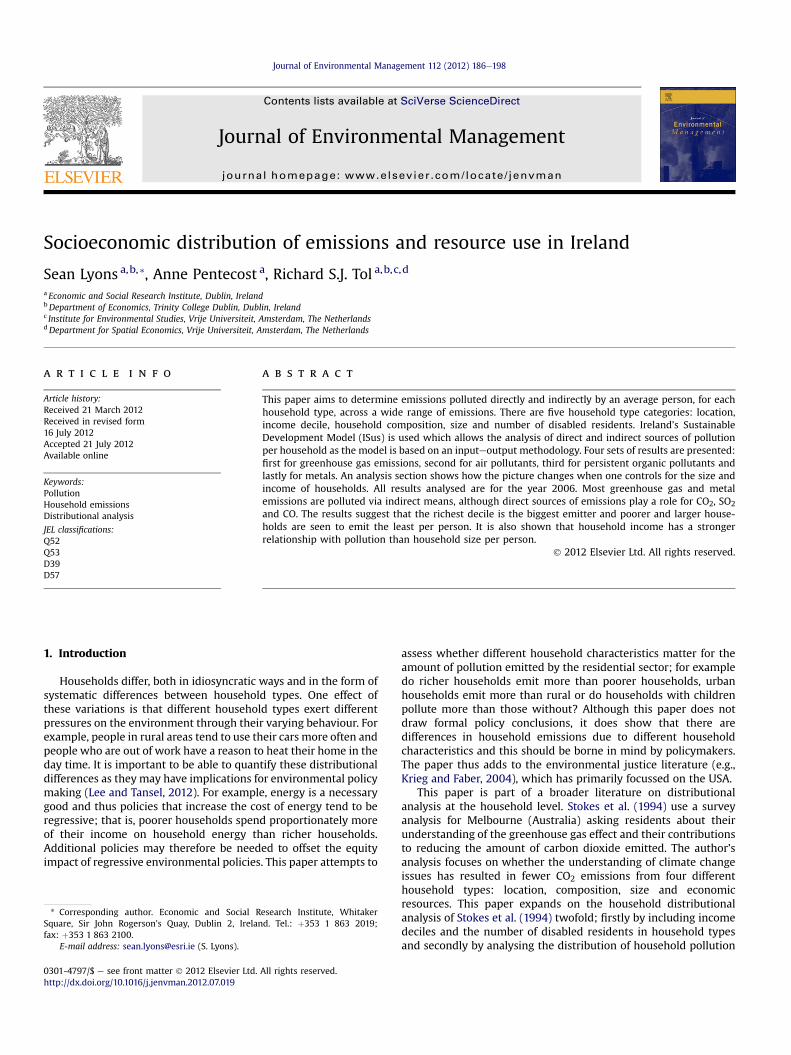
Fig. 5. Direct and indirect emissions of Nitrous Oxide (N2O) per person by household type.


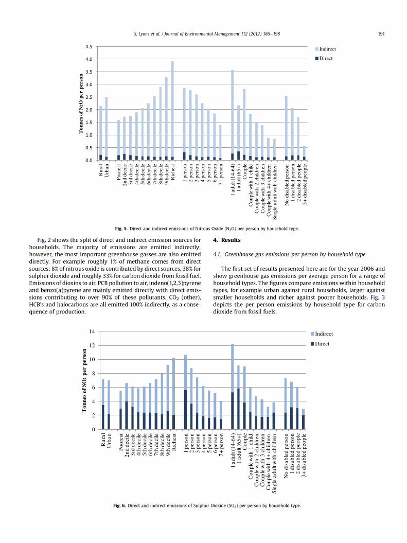
Fig. 2 shows the split of direct and indirect emission sources forhouseholds. The majority of emissions are emitted indirectly;however, the most important greenhouse gasses are also emitteddirectly. For example roughly 1% of methane comes from directsources; 8% of nitrous oxide is contributed by direct sources, 38% forsulphur dioxide and roughly 33% for carbon dioxide from fossil fuel.Emissions of dioxins to air, PCB pollution to air, indeno(1,2,3)pyreneand benzo(a)pyrene are mainly emitted directly with direct emis-sions contributing to over 90% of these pollutants. CO2 (other),HCB’s and halocarbons are all emitted 100% indirectly, as a conse-quence of production.

0

2

4

6

8

10

12

14

Rur

alU

rban

Poor

est

2nd

deci

le3r

d de

cile

4th

deci

le5t

h de

cile

6th

deci

le7t

h de

cile

8th

deci

le9t

h de

cile

Ric

hest

1 pe

rson

2 pe

rson

3 pe

rson

4 pe

rson

5 pe

rson

Ton

nes

of S

O2

per

pers

on

Fig. 6. Direct and indirect emissions of Sulphur D

4. Results

4.1. Greenhouse gas emissions per person by household type

The first set of results presented here are for the year 2006 andshow greenhouse gas emissions per average person for a range ofhousehold types. The figures compare emissions within householdtypes, for example urban against rural households, larger againstsmaller households and richer against poorer households. Fig. 3depicts the per person emissions by household type for carbondioxide from fossil fuels.

6 pe

rson

7+ p

erso

n

1 ad

ult (

14-6

4)1

adul

t (65

+)C

oupl

eC

oupl

e w

ith 1

chi

ldC

oupl

e w

ith 2

chi

ldre

nC

oupl

e w

ith 3

chi

ldre

nC

oupl

e w

ith 4

+ ch

ildre

nSi

ngle

adu

lt w

ith c

hild

ren

No

disa

bled

per

son

1 di

sabl

ed p

erso

n2

disa

bled

peo

ple

3+ d

isab

led

peop

le

Indirect

Direct

ioxide (SO2) per person by household type.

0

5

10

15

20

25

30

35

40

Rur

alU

rban

Poor

est

2nd

deci

le3r

d de

cile

4th

deci

le5t

h de

cile

6th

deci

le7t

h de

cile

8th

deci

le9t

h de

cile

Ric

hest

1 pe

rson

2 pe

rson

3 pe

rson

4 pe

rson

5 pe

rson

6 pe

rson

7+ p

erso

n

1 ad

ult (

14-6

4)1

adul

t (65

+)C

oupl

eC

oupl

e w

ith 1

chi

ldC

oupl

e w

ith 2

chi

ldre

nC

oupl

e w

ith 3

chi

ldre

nC

oupl

e w

ith 4

+ ch

ildre

nSi

ngle

adu

lt w

ith c

hild

ren

No

disa

bled

per

son

1 di

sabl

ed p

erso

n2

disa

bled

peo

ple

3+ d

isab

led

peop

le

Ton

nes

of C

O p

er p

erso

n

Indirect

Direct

Fig. 7. Direct and indirect emissions of Carbon Monoxide (CO) per person by household type.


The average person in a rural household emits more CO2 directlythan an average person in an urban household; however an averageurban household emits more CO2 indirectly and also more in totalthan an average person in a rural household. Direct emissions inrural areas could be due to transport for example as cars are usedmore in rural areas whereas public transport is used more in urbanareas. The definition of ‘rural’ used here includes much of thecommuter belt. Indirect emissions could result from the productionof household energy by power plants.

The poorest households emit the least CO2 both directly andindirectly with nearly 1400 tonnes and 1900 tonnes per personrespectively, and the richest households emit the most CO2 bothdirectly (1985 tonnes) and indirectly (6224 tonnes) per person

0

1

2

3

4

5

6

7

8

Rur

alU

rban

Poor

est

2nd

deci

le3r

d de

cile

4th

deci

le5t

h de

cile

6th

deci

le7t

h de

cile

8th

deci

le9t

h de

cile

Ric

hest

1 pe

rson

2 pe

rson

3 pe

rson

4 pe

rson

5 pe

rson

Ton

nes

of N

MV

OC

per

per

son

Fig. 8. Direct and indirect emissions of Non-me

and thus the richest decile emits 4900 tonnes more in total thanthe poorest decile. The increase in each decile for indirect emis-sions seems to be more an exponential growth than a linear one.The larger the household the less CO2 is produced per person,with decreases in indirect, direct and thus total emissions ashouseholds get bigger. This is consistent with the presence ofeconomies of scale in consumption; where household activities,for example cooking, are undertaken for the whole householdrather than by each individual and thus emissions per person areless for households with more people. The only anomaly is fora retired aged single adult; for a single adult it is expected thattotal emissions would higher than a for a couple, however this isnot the case and results suggest a couple emits 999 tonnes more

6 pe

rson

7+ p

erso

n

1 ad

ult (

14-6

4)1

adul

t (65

+)C

oupl

eC

oupl

e w

ith 1

chi

ldC

oupl

e w

ith 2

chi

ldre

nC

oupl

e w

ith 3

chi

ldre

nC

oupl

e w

ith 4

+ ch

ildre

nSi

ngle

adu

lt w

ith c

hild

ren

No

disa

bled

per

son

1 di

sabl

ed p

erso

n2

disa

bled

peo

ple

3+ d

isab

led

peop

le

Indirect

Direct

thane VOC per person by household type.

0

5

10

15

20

25

30

35

40

Rur

alU

rban

Poor

est

2nd

deci

le3r

d de

cile

4th

deci

le5t

h de

cile

6th

deci

le7t

h de

cile

8th

deci

le9t

h de

cile

Ric

hest

1 pe

rson

2 pe

rson

3 pe

rson

4 pe

rson

5 pe

rson

6 pe

rson

7+ p

erso

n

1 ad

ult (

14- 6

4)1

adul

t (65

+)C

oupl

eC

oupl

e w

ith 1

chi

ldC

oupl

e with

2 c

hild

ren

Cou

ple

with

3 c

hild

ren

Cou

ple

with

4+

child

ren

Sing

le a

dult

with

chi

ldre

n

No

disa

bled

per

son

1 di

sabl

ed p

erso

n2

disa

bled

peo

ple

3+ d

isab

led

peop

le

g T

EC

of d

ioxi

n pe

r pe

rson

Indirect dioxins (land)

Direct dioxins (land)

Indirect dioxins (air)

Direct dioxins (air)

Fig. 9. Direct and indirect emissions of Dioxins per person by household type.


than an average retired adult. This could be due to an averagecouple having a higher income than an average single retiredperson.

Fig. 4 shows per average person emissions for methane (CH4)where almost all household emissions of this gas are indirect.

Direct household methane emissions originate mainly fromhousehold waste and compost and sources of indirect methaneemissions are landfill sites, for example. It is clear that, indi-rectly, urban households emit more per person than ruralhouseholds by 10 tonnes but rural households emit more perperson than urban households by 0.2 tonnes from direct sources.

0

1

2

3

4

5

6

7

8

9

Rur

alU

rban

Poor

est

2nd

deci

le3r

d de

cile

4th

deci

le5t

h de

cile

6th

deci

le7t

h de

cile

8th

deci

le9t

h de

cile

Ric

hest

1 pe

rson

2 pe

rson

3 pe

rson

4 pe

rson

5 pe

rson

6 pe

rson

Kgs

of P

b, H

g an

d C

d pe

r pe

rson

Fig. 10. Indirect emissions of Lead (Pb), Mercury (Hg) a

The richer the average person becomes the higher the indirectemissions (and the lower the direct emissions), and this increaseseems to be more exponential rather than linear. The differencebetween indirect and direct emissions for the richest decile is85 tonnes.

One and two person households emit roughly the same quantityof methane per person indirectly, however a one person householdemits more than any other household size by direct sources (a oneperson household emits 1 tonne directly whereas a two personhousehold emits 0.6 tonnes and a seven or more person householdemits 0.2 tonnes from direct sources). The larger the household the

7+ p

erso

n

1 ad

ult (

14-6

4)1

adul

t (65

+)C

oupl

eC

oupl

e w

ith 1

chi

ldC

oupl

e w

ith 2

chi

ldre

nC

oupl

e w

ith 3

chi

ldre

nC

oupl

e w

ith 4

+ ch

ildre

nSi

ngle

adu

lt w

ith c

hild

ren

No

disa

bled

per

son

1 di

sabl

ed p

erso

n2

disa

bled

peo

ple

3+ d

isab

led

peop

leIndirect Lead

Indirect Mercury

Indirect Cadmium

nd Cadmium (Cd) per person by household type.

0

5

10

15

20

25

30

35

40

45

Rur

alU

rban

Poor

est

2nd

deci

le3r

d de

cile

4th

deci

le5t

h de

cile

6th

deci

le7t

h de

cile

8th

deci

le9t

h de

cile

Ric

hest

1 pe

rson

2 pe

rson

3 pe

rson

4 pe

rson

5 pe

rson

6 pe

rson

7+ p

erso

n

1 ad

ult (

14-6

4)1

adul

t (65

+)C

oupl

eC

oupl

e w

ith 1

chi

ldC

oupl

e w

ith 2

chi

ldre

nC

oupl

e w

ith 3

chi

ldre

nC

oupl

e w

ith 4

+ ch

ildre

nSi

ngle

adu

lt w

ith c

hild

ren

No

disa

bled

per

son

1 di

sabl

ed p

erso

n2

disa

bled

peo

ple

3+ d

isab

led

peop

le

Kgs

of C

u, C

r an

d N

i pe

r pe

rson

Indirect copper

Indirect chromium

Indirect nickel

Fig. 11. Indirect emissions of Copper (Cu), Chromium (Cr) and Nickel (Ni) per person by household type.


less is emitted per person both from indirect and direct sources,making smaller households bigger emitters. A similar pattern holdsfor household composition for both direct and indirect emissions;single adults and couples are the largest emitters per person andemissions fall the more children are in the household. A workingaged adult emits the most indirectly with 76 tonnes and a retiredadult emits the most directly at 1.3 tonnes. Again the pattern issimilar for the number of disabled people in a household; the moredisabled people the less emissions per person from indirect sour-ces. This, however, is not the same for direct emissions; emissionsfrom direct sources increase with the number of disabled people,amounting to 0.6 tonnes for two disabled people whereas with nodisabled person in a household the average per person emission ofmethane is 0.4 tonnes. Emissions do fall, however, when there areat least three disabled people in a household to just over 0.4 tonnes.

0

50

100

150

200

250

300

350

400

450

500

Rur

alU

rban

Poor

est

2nd

deci

le3r

d de

cile

4th

deci

le5t

h de

cile

6th

deci

le7t

h de

cile

8th

deci

le9t

h de

cile

Ric

hest

1 pe

rson

2 pe

rson

3 pe

rson

4 pe

rson

5 pe

rson

Kg

of Z

n pe

r pe

rson

Fig. 12. Indirect emissions of Zinc (Zn

A detailed graph of direct emissions of methane (and other emis-sions) can be found in the Appendix (Fig. A1), although roughly 99%of methane emissions come from indirect sources as shown byFig. 2.

Fig. 5 depicts emissions of nitrous oxide per person by house-hold type. Direct household emissions of N2O could be a conse-quence of fossil fuel use from driving and indirect emissions couldarise from the use of fertilisers or the incineration of householdwaste, for example. Nitrous oxide emissions are mostly emittedindirectly, with the richest income decile emitting the most (thedifference between direct and indirect emissions is roughly3.5 tonnes for the richest decile). The more people in the house-hold, the less emissions per person both indirectly and directly; forone and two person households the average person emits similaramounts indirectly (2.37 and 2.35 tonnes respectively), however

6 pe

rson

7+ p

erso

n

1 ad

ult (

14-6

4)1

adul

t (65

+)C

oupl

eC

oupl

e w

ith 1

chi

ldC

oupl

e w

ith 2

chi

ldre

nC

oupl

e w

ith 3

chi

ldre

nC

oupl

e w

ith 4

+ ch

ildre

nSi

ngle

adu

lt w

ith c

hild

ren

No

disa

bled

per

son

1 di

sabl

ed p

erso

n2

disa

bled

peo

ple

3+ d

isab

led

peop

le

Indirect zinc

) per person by household type.


a two person household emits less directly than a one personhousehold.

Urban households emit more nitrous oxide indirectly by0.3 tonnes. Rural households emit more directly, although thisdifference is a lot smaller. For a household with three or moredisabled people, the average person per household emits lessnitrous oxide than other other household type (the differencebetween direct and indirect emissions is also the smallest). A moredetailed graph of direct emissions of N2O can be found in theAppendix (Fig. A2).

4.2. Air pollutants per person by household type

Fig. 6 shows emissions from both direct and indirect sources ofsulphur dioxide (SO2) for an average person in each household type.The largest source of indirect SO2 pollution is from fossil fuelcombustion in power plants (for example burning coal to provideelectricity). Direct emission sources of SO2 include car emissionsfrom fuel combustion.

Direct emissions per person fall gradually as household incomeincreases,whereas indirect emissions increase sharplywith income.The average person in an urban household emits more by indirectmeans than an average rural residing person; however this patternis reversed with direct emissions. In contrast, indirect emissions areroughly constant across household sizes, while direct emissions perperson are lower for larger households. Similar total emissions forurban and rural households mask differing composition, with ruralhouseholds having relatively more direct emissions.

In Fig. 7 we show the distribution of carbonmonoxide emissionsper average person for different household types. Direct emissionscould result from car exhausts and lawn mowers with internal

0.

0.

1.

1.

2.

2.

3.

3.H

PCB (air)Dioxin (land)

Halocarbons

Dioxin (air)

CO2 (fossil)

NOx

CO2 (other)

Dioxin (water)

Benzo(k)fluoranthene

Benzo(b)fluoranthene

Benzo(a)pyrene

PCB (land)

CO

Indeno(1,2,3)pyrene

NMVOC

Fig. 13. Income intensity of emissions: ratio of household emissions per person for

combustion engines; an indirect source is the burning of fossil fuelsin power plants.

A working aged single person generates the most carbonmonoxide and a couple with at least four children emits theleast carbon monoxide. Again direct emissions play a significantrole although for most households per person emissions aremainly from indirect sources. The patterns are similar to thoseanalysed before; the richest decile is the biggest emitter quan-tified as 30 tonnes and the more people per household, thelower emissions per person become. For rural households, thepoorest three income deciles, a one person household, a retiredsingle adult, a couple with 4 children, a single parent andhouseholds with at least two disabled people, per personemissions are greater from direct sources than indirect sources.The highest emission per person from direct sources is fora retired adult (23 tonnes) and the smallest for a seven personhousehold at just under 5 tonnes. This is similar to the resultsfor sulphur dioxide and carbon dioxide but substantiallydifferent from the other gas emissions.

Fig. 8 shows direct and indirect sources of emissions forNMVOC; the former resulting from the vapour emitted from carexhausts and solvent use and the latter as a consequence ofextraction and distribution of fossil fuels. A retired adult and anaverage household with at least three disabled residents in emitmore NMVOC directly than indirectly. The rich emit more indi-rectly and in total than the poor, however, the poor emit moredirectly than the rich. For both indirect and direct channels ofemissions, the larger the household the lower emissions perperson. This is consistent with household composition where themore children there are in a household, the lower emissions perperson.

0

5

0

5

0

5

0

5CB (water)

HCB (land)

HCB (air)

NH3

CH4

BOD

N2O

Copper

Zinc

Lead

Cadmium

Chromium

Mercury

SO2

ArsenicNickel

Direct

Indirect

those in the highest income decile to those in the lowest decile by substance.

0.0

0.1

0.2

0.3

0.4

0.5

0.6

0.7

0.8PCB (land)

HCB (water)

HCB (land)

HCB (air)

NH3

CH4

N2O

BOD

Halocarbons

Cadmium

Lead

Mercury

Arsenic

SO2

NickelChromiumCopper

PCB (air)

Zinc

CO2 (fossil)

NOx

Dioxin (land)

Dioxin (air)

Benzo(k)fluoranthene

CO2 (other)

Benzo(b)fluoranthene

Benzo(a)pyrene

NMVOC

CO

Indeno(1,2,3)pyrene

Dioxin (water)Direct

Indirect

Fig. 14. Household intensity of emissions: ratio of household emissions per person the largest households (6 persons) to those in the smallest (one person) by substance.


4.3. Persistent organic pollutant emissions per person by householdtype

Fig. 9 shows direct and indirect emissions of dioxins which gointo land and air. Emissions of dioxins into water, which arenegligible in quantity, can be found in the Appendix (A6).

Urban and rural households emit roughly the same of each typeof dioxins. The richer deciles emit less than poorer deciles in total,which stands in contrast to every other emissionwe studied. Poorerhouseholds emit larger quantities directly, perhaps due to greateruse of open fireplaces, wood stoves and coal fired utility boilers. Therichest deciles do, however, emit more indirectly into land than thepoorer deciles. An indirect source of dioxin pollution is through theproduction of chemical and pesticides. Bigger households polluteless than smaller households per person, as found for other emis-sions. If up to two disabled people reside in the household, emis-sions are higher than for three or more disabled people which isalso different from the gas emissions previously analysed whereemissions fall for each additional disabled resident.

4.4. Metal emissions per person by household type

We have data only for metal emissions via indirect channels byhouseholds and thus we do not show any direct pollution fromhouseholds for the metal pollutants examined. Indirect metalemissions mainly are a result of municipal waste incineration, fossilfuel combustion for example pollution from power stations, andindustrial processes such as pulp and paper manufacturing.

Fig. 10 depicts the indirect emissions per person by householdtype for three metals, namely lead, mercury and cadmium. Thepatterns of the results are essentially the same for these emissions,so we analyse them together.

Urban households emit more than rural households, the rich-est deciles emit more than the poorer deciles and the larger thehousehold the lower emissions are per person. Households withup to three residents emits roughly the same quantities perperson of lead, mercury and cadmium, which is slightly differentfrom the pattern observed for gas emissions where two and threeperson households emitted visibly less than one person house-holds. Of the three metals, the least cadmium and the mostmercury are emitted by households. Cadmium is emitted is themanufacturing of electrical equipment, and it is also found incigarettes. Most mercury pollution form households is fromproduction (of non-ferrous metal and cement for example), but itis also from waste disposal.

Fig. 11 shows the indirect emissions by household type forcopper, chromium and nickel. Once again, we group these metalstogether because their patterns are similar.

Urban households emit more than rural households, the richerincome deciles emit more than the poorer deciles and the larger thehousehold size the fewer emissions per person. For all emissionsthe richest decile is the biggest emitter and a household with atleast three disabled residents are the smallest emitters with thedifference being 38 kg, 26 kg and 24 kg for copper, chromium andnickel respectively.

In Fig. 12 we show the indirect emissions by household type forzinc. Urban households emit more than rural households, the richerdeciles emit more than the poorer deciles and the larger thehousehold the less are emissions per person. The richest decileemits the most (436 kg) and a household with at least threedisabled residents emits the least (46 kg). The difference betweenthe richest and the poorest is 300 kg. The difference between perperson emissions of a single adult with children and a single adultof working age without children is on a similar scale: 292 kg.


5. Analysis

In this section we consider how household income and size areassociated with emissions of the substances covered in the paper.Household income and size are analysed as these household typeshave a clearer policy focus than location or household composition.4

Fig. 13 depicts the relationships that direct and indirect emissionshave with income: the emissions ratio of the richest decile to thepoorest decile. For each emission, this is per person pollutionemitted directly (indirectly) for the richest household income deciledivided by per person pollution emitted directly (indirectly) for thepoorest income decile. Thus an emission with a high ratio is onewhere emissions are strongly related to income, whereas low ratiosindicate emissions with little association with income.

HCB (emitted to water) is shown to have the lowest ratio bothindirectly and directly. Top earning households cause only 2.6 timesthe per capita indirect emissions that low earning households do.Non-methane volatile organic compounds (NMVOC) have thehighest ratio for indirect emissions (almost 3.5) and oxides ofnitrogen (NOx) have the highest for direct emissions. Only NOx andCO2 from fossil fuels have a ratio of more than 1 for direct emis-sions. Ceteris paribus, policies that affect the cost of direct emissionsare likely to be much more regressive than those affecting indirectemissions.

Fig. 14 illustrates the association between household size andemissions: the emissions ratio of the largest household size to thesmallest household size. This is calculated as the per personpollution of direct (indirect) emissions for a six person householddivided by the per person pollution of direct (indirect) emissionsfor a one person household, for each emission.

Pollutants show a very similar pattern, with an average ratio of0.68. Again oxides of nitrogen (NOx) have the highest direct emis-sions ratio and PCB (pollution to land) has the lowest. Size ratios aregenerally lower than the income ratios discussed above; in Fig. 14no emission has a ratio over 0.7; however in Fig. 13 all indirectemissions ratios and two of the direct emissions ratios are over 1.Income has a much stronger association with household emissionsper person than household size does.

6. Conclusion

This paper has reported estimates of Ireland’s direct and indirectemissions per capita by household type for a range of pollutants.Households are split in five ways, by location, income decile,composition, size and the number of disabled residents. This wasdone for indirect emissions using inputeoutput modelling and fordirect emissions (where relevant) by applying emission factors tomicrodata from an expenditure survey.

The results show that most pollution comes from indirectsources; in fact for the greenhouse gases, direct sources nevermakeup more than 35% of household emissions per person. In general,richer deciles tend to pollute more than poorer deciles; howeverdioxins seem to be an exception to this pattern. Another commonfeature is that the larger the household the less pollution perperson. Urban households tend to pollute more than rural house-holds except for emissions of carbon monoxide and sulphurdioxide, which probably has to do with differences in the averagehousehold fuel mix. For emissions of CO2, N2O and CH4, indirectsources play a more important role than direct sources of emis-sions, whereas for emissions CO and SO2, direct emission sourcesare relatively more important.

4 The incidence of a carbon tax, for example, would tend to be correlated withhousehold income and size, rather than household composition or location.

For metals we have estimated emissions only for the indirectchannel. Zinc is emitted the most by households of all the metalsfollowed by copper. Cadmium is emitted the least. The patterns byhousehold type are similar across the various metals, and they arenot dissimilar to those found for the gases. There are some subtledifferences; for example, for the metal emissions a household of upto three residents emit a fairly equal share, however, for the gasemissions a two person household emits visibly less than a oneperson household and a three person household again visibly emitsless than a two person household.

We also noted that household size has aweaker associationwithboth direct and indirect emissions than household income does.Variations in indirect emissions are much more strongly associatedwith income than direct emissions, implying that a similarproportional change in the cost of emissions would be moreregressive if applied to direct emissions than to indirect emissions.

The impact of environmental policy will tend to have differingincidence across households, to the extent that household typeshave differing emission patterns. This non-homogeneity hasimplications for environmental policy, because measures that raisethe cost of emitting a pollutant (e.g., a tax or regulatory restriction)will fall more heavily on some households than others. If thissignificantly affects vulnerable households or changes the distri-bution of taxation in a material way, it may be necessary to offsetthe impact through appropriate tax or benefit measures. Furtherworkwould be to estimate a regression equation in order to predictemission levels of the different household types and to determinethe relative contribution of household types for emissions.

Acknowledgements

We are grateful for funding under the EPA Strive Programme,and we would like to thank Anne Jennings for excellent researchassistance and participants at the May 2011 ESRI/EPA seminar onEnvironmental Economics for helpful comments on an earlierversion of this paper. The usual disclaimer applies.

Appendix A. Supplementary data

Supplementary data related to this article can be found online athttp://dx.doi.org/10.1016/j.jenvman.2012.07.019.

References

Creedon, M., O’Leary, E., Thistlewaite, G., Wenborn, M., Whiting, R., 2010. Invento-ries of Persistent Organic Pollutants in Ireland 1990 and 1995e2006, ClimateChange Research Programme (CCRP) 2007e2001 Report Series No. 2.

CSO, 2006. 2000 Supply and Use and InputeOutput Tables. Central Statistics Office,Cork.

CSO, 2007. Household Budget Survey 2004e2005: Final Results. Central StatisticsOffice, Cork.

CSO, 2010. Environmental Accounts for Ireland. Central Statistics Office, Cork.Duffy, P., Hyde, B., Hanley, E., Dore, C., O’Brien, P., Cotter, E., Black, K., 2011. Ireland

National Inventory Report Greenhouse Gas Emissions 1990e2009, Reported tothe United Nations Framework Convention on Climate Change.

Ferreira, S., Moro, M., 2011. Constructing genuine savings indicators for Ireland,1995e2005. Journal of Environmental Management 92, 542e553.

Hassett, K., Mathur, A., Metcalf, G., 2007. The Incidence of a U.S. Carbon Tax:a Lifetime and Regional Analysis, NBER Working Paper No.13554.

Hayes, F., Murnane, I., 2002. Inventory of Dioxin and Furan Emissions to Air, Landand Water in Ireland for 2000 and 2010, EPA Environmental RTDI Programme2000e2006, Report 3.

Integrated Pollution Prevention Control (IPPC), EPA 2011. Data taken from: http://www.epa.ie/whatwedo/licensing/ippc/. Accessed 12 May 2011.

Krieg, E.J., Faber, D.R., 2004. Not so black and white: environmental justice andcumulative impact assessments. Environmental Impact Assessment Review 24,667e694.

Labandeira, X., Labeaga, J., 1999. Combining inputeoutput analysis and micro-simulation to assess the effects of carbon taxation on Spanish households.Fiscal Studies 20, 305e320.


http://www.epa.ie/whatwedo/licensing/ippc/

http://www.epa.ie/whatwedo/licensing/ippc/


Lee, M., Tansel, B., 2012. Life cycle based analysis of demands and emissions forresidential water-using appliances. Journal of Environmental Management 101,75e81.

Parikh, A., 1979. Forecasts of inputeoutput tables using the RAS method. Review ofEconomics and Statistics 61, 477e481.

Scott, S., 1999. Compilation of Satellite Environment Accounts, Working Paper 116,Economic and Social Research Institute, Dublin.

Stokes, D., Lindsay, A., Marinopoulos, J., Treloar, A., Wescott, G., 1994. Householdcarbon dioxide production in relation to the greenhouse effect. Journal ofEnvironmental Management 40, 197e211.

Symons, E., Proops, J., Gay, P., 1994. Carbon taxes, consumer demand and carbondioxide emissions: a simulation analysis for the UK. Fiscal Studies 15, 19e43.

Verde, S., Tol, R., 2009. The distributional impact of a carbon tax in Ireland. TheEconomic and Social Review 40, 317e338.

socioeconomic distribution of emissions and resource use in ireland

Documents