PHYSICAL REVIEW

VOLUME 171, NUMBER 3

15 JULY 1968

Helicon Waves, Surface-Mode Loss, and the Accurate Determinationof the Hall Coefficients of Aluminum , Indium,

Sodium and Potassium*

JOHN M. GOODMAN+Laboratory of Atomic and Solid Slate Physics, Cornell University, Ithaca, New York,

and Harvey Mudd College, Claremont California(Received 23 January 1968)

Observations of helicon wave resonances in some metals have been interpreted by various investigatorsas implying values for the Hall coefficients of these metals which a re significantly higher than the theoreticalvalues . This interpretation resulted from using an approximate solution to the relevant boundary-valueproblem, without a full appreciation of the extent of the errors which were thereby incurred . In 1961,Legendy critically discussed the boundary conditions and gave several solutions . His solution for an infinitecylinder parallel to the. static magnetic held is particularly interesting in that it predicts the existence ofa surface mode whose total power dissipation is virtually independent of the resistivity of the material .This paper presents a detailed quantitative experimental confirmation of the accuracy of this solution,thus validating the boundary condition used . The observations also yield values for the Hall coefficientsof aluminum, indium, sodium, and potassium which are equal to the theoretical values to within the experi-mental accuracy of about 1/2 %.

I. INTRODUCTION

In 1962, Chambers and Jones showed that the heli-con-wave (magnetoplasma) resonance frequencies

andline shapes which occur for a sample could be pre-dicted from a knowledge of its Hall coefficient, resis-tivity, and shape, and from the geometry of the exci-tation and detection coil system. They suggested thatthe observation of helicon resonances could thereforebe used to measure the Hall coefficients of a widevariety of materials, in particular, the simple metals atlow temperatures. Since this method differs from theconventional one in permitting rather larger sample di-mensions and in substituting a frequency measurementfor voltage and current measurements, it would appear

This work was mainly supported by the U . S . Atomic EnergyCommission under Contract No. AT(30-l)-2150, Technical Re-port No . NYO-2150-44, Substantial help was received from theAdvanced ResearchProjects Agency through the use. of theCentral Facilities of the Mateials Science Center at CornellUniversity, MSC Report No. 963. .

t Danforth and National Science Foundation Graduate Fellow,1950-65 . Present address : >iuney Mudd Cohere, t iare .nc,nt,Cciif . 91711 .

1 b: . G. Chambers and B . K. Tones, Proc . Roy. Soc . (London)A270, 417 t!962).

to be capable of substantially higher accuracy . They alsopointed out that the theory of metals makes a clearprediction for the high-field linm.iting value of the Hallcoeffilcient in metals with a closed Fermi s~,rfice . \'; enthey attempted to interpret their helicon-resonanceobservations on samples of lithium, SOdlii_'27, p ;iaSSii'L? .allmiinuni, and indium in terms of the sample materials'Hall coefficients, however, they obtained values htc_twere svsternaticallv about 5% high with an experi-mental uncertainty of only about 1% .

Since the resonance is evidence of a standing wavepattern in the sample, its frequency can be used todetermine the sample material's Hall coefficient onlyone has a sufficiently accurate solution to the helicon-wave-boundary-value problem relevant to the partir-a-lar sample and coil geometry used . Chambers and Jonesanalyzed the case of a thin slab perpendicular tostatic magnetec field, assuming no variation of the wavefields in the transverse directions could occur

only in a plate whose transverse dimensions wereinfinite). Their principal conclusion was that resonanceoccurs when the sample thickness is an integral numberof half-wavelengths. They calculated an approximate

642

correction to be applied for a finite sample, but it wasnot sufficient to remove the discrepancy in the Hallcoefficients .

Guided by the theoretical result of Chambers andJones and by the analogy to a microwave cavity, Rose,Taylor, and Bowers' calculated the Hall coefficient ofsodium from experimental data on variously propor-tioned rectangular samples, using the infinite-mediumhelicon-wave dispersion relation and assuming integralhalf-wavelengths in each of the sample dimensions atresonance. This ad hoc assumption about the form of thesolution to the boundary-value problem led to veryaccurate predictions of the relative frequencies of thevarious helicon-wave modes, as was more accuratelydemonstrated by Merrill, Taylor, and Goodman, 3 butthe absolute value of the Hall coefficient again came outabout 5o higher than the theoretical value .

In several attempts to solve the boundary-valueproblem, the assumption was made that a linear combi-nation of plane-wave solutions for the infinite ,mediumwhich resulted in no current flow across the boundariesof the finite sample represented an adequate approxi-mation to the true solution . In 1964, Legendys gave acritical discussion of this and other proposed boundaryconditions, concluding that the appropriate boundarycondition was simply the continuity of all components ofthe magnetic field at the boundary (for low enoughfrequencies that the external wave fields could be con-sidered quasistatic). He also gave exact solutions to theboundary-value problem for several simple semi-infinitegeometries .

In this paper, we shall be particularly concerned withLegendy's solution for an infinite cylindrical sampleparallel to the static magnetic field and subjected to adriving field which is periodic in both time and space .In this situation two helicon modes with strikingly dif-ferent properties are excited in the material . One is thefamiliar helicon wave which propagates freely insidethe material in the limit of infinite conductivity . Thismode is responsible for the standing-wave phenomenaobservable in this case . The other mode decays exponen-tially away from the surface with a damping lengthwhich is inversely proportional to the conductivity. Asurprising consequence of this dependence on distanceand resistivity is that the total power dissipation in thismode is independent of the resistivity of the samplewithin broad limits .

This result can most easily be seen by the followingsimple order-of-magnitude calculation . The total powerloss per unit area can be estimated by its magnitude atthe surface, j 2p, times the effective skin depth 5, inwhich the fields and currents fall to e -1 of their surfacevalues. But the current density is just the c rrl of the

2 F. F. Rose, M . T . Taylor, and R . Bowers . Phvs . Rev. 127,1122 (1962) .3 J. R Merrill, M. T . Taylor, and J . M. Goodman, Phys . Rev .131, 2499 (1963) .

4 C. R. Legendy, Phys. Rev. 135, A1713 (1964).

JOHN IM . GOODMAN 171

magnetic field of the wave, which, for a mode exhibitinga simple exponential decay, is siripl equal to the ampli-tude of the wave's magnetic field divided by the skindepth . Thus, in this case, the total loS.s is just propor-tional to the square of the wave field amplitudetimes p,.'5 . In the ordinary skin effect, S is proportionalto pi/ 2, so that the total power loss is also proportionalto pr" 2 , but for this mode, with o w p, the loss is indepen-dent of the resistivity .The first observations of this surface loss were

reported by Goodman'' and by Harding and Thone-manns in 1965. The former was a. preliminary report ofthe work described in this paper ; the latter reported theobservation of the surface loss in a slightly differentexperiment . Klozenherg, McNamara, and Thonemann'calculated the properties of a cylindrical sample parallelto the static magnetic field considered as a helicon wave-guide, using continuity of the magnetic field of the waveas the boundary condition . (This differs from Le'Dg6ndy'swork only in the absence of a driving field along thesurface .) They also noted the existence and propertiesof the surface mode . Harding and Thonemamn .reportedexperimental measurements on the phase shift andamplitude as a function of distance of a helicon wavelaunched down an indium bar from one end . They alsonoted that the observed phase velocity could be inter-preted to yield a . value for the Hall coefficient of indiumwhich was equal to the theoretical value to within theiraccuracy of about 1 .5,70 .

Recently, Baraff and Buchsbaum have shown theo-retically that the corresponding helicon surface mode incertain multilayered structures can cause a net powergain for a sufficiently large drift current . This amplifierpotential makes an experimental confirmation of thesurface-mode properties even more interesting .

In this paper, a detailed experimental test of the ac-curacy of Legendy's cylinder solution is described. Theresults demonstrate all of the basic properties of thesolution, including quantitative agreement with theamount of power disipation predicted in cases wherevirtually all of the loss is in the surface mode, thusclearly confirming its existence and major character-istics . The results also indicate that the Hall coefficientsof the sample materials, sodium, potassium, aluminum,and indium, are equal to the theoretical values to withinthe accuracy with which they could be determined inthis experiment, with the possible exception of sodium .

A related piece of work which should be mentionedwas published recently by Amundsen.' He studied the

5 J. M. Goodman, Bull. Am. Phys. Soc. 10, 111 (1965).6 G. N. Harding and P . C. Thonemann, Proc. Phys. Soc .(London) 85, 317 (1965) .7 J . P . Klozenbcrg, B . McNamara, and P . C. Thonemann, J .Fluid Mech . 21, 545 (1965) .8 . G. A. Baraff and S. J. Buehsbaum, Appl. Phys. Letters 6,219 (1965) Phys . Rev . 111,. 266 (1966) ; see also L . M. Saunders,G. A . Baraff, and S . J. Buchsbaum, J, Appl. Phys . 37, 2935(1966) .

9T. Amundsen, Proc. Phys. Soc. (London) 58, 757 (1966) .

171

I-IALL COEFFICIENTS OF A1, In, Na, AND K

643

dependence of the resonant frequencies of a sequence ofthin indium slabs placed perpendicular to the staticmagnetic field on the ratio of their lateral to axial di-mensions. He demonstrated agreement with the de-pendence derived from Legendy's solution for this case,and by extrapolating his results to infinite lateraldimensions and using the theory of Chambers and Jones,he obtained a value for the high-field limit of the Hallcoefficient of indium which is equal to the theoreticalvalue to within his accuracy of about 1 .5% .

In Sec. II, the experimental arrangement is de-scribed and the nature of the phenomena to be expectedis discussed . In Sec . III, the theoretical calculations areoutlined, the physical assumptions briefly discussed, anda useful approximate model described . These arefollowed by sections dealing with the experimentalapparatus and samples used . The observations and thefitting of the theory to them are discussed in the finalsections . The detailed development of the theoreticalmodel is given in the Appendix .

II. NATURE OF THE EXPERIMENT

The experimental arrangement to be discussed is in-cated in Fig . 1 . A cylindrical metal sample of radiusis aligned parallel to the static magnetic field B 0. It issurrounded by two coaxial coils of radii d and D, eachconsisting of 20 sections . The direction of the windingsin each section is opposite to that in the neighboringsections . A sinusoidal current A coswi in one of the coilssets up a magnetic field which can be thought of as thesum of two waves of wavelength a traveling in oppositedirections along the sample with velocity wX/2 ;r. Withthis particular coil geometry, the linear dimensionwhich is most important in determining the frequency ofthe standing helicon-wave resonances is the wave-length of the coil rather than a sample dimension . Thepenetration of this wave field into the sample can beobserved by measuring the mutual inductance betweenthe coils . Measurements of the loss part of this induc-tance, called the mutual resistance, will reflect the powerdissipation in the sample . If the secondary-coil voltageis V(1) and the primary current is A coswt, the mutual

Fir . 2 . 'Mutual inductance and resistance versus drive-currentfrequency for a potassium sample K(1). B,)=35 k0. The experi-mental data are represented by plus signs . The solid curve iscalculated from Eq . (A17) . The dashed curve is the theoreticalprediction for an infinitely long coil systern. . :lfo is the calculatedinductance of the coil without a sample . This and the ether graphsare photoreproductions of the computer output .

inductance M and mutual resistance R are defined by

V(t)=A(R coswt+w lj' sinwi) . (2 .1)

The experiment consists of the measurement of Mand R as functions of the frequency v (=w/2a-) for anumber of different static-magnetic-field strengths andsample materials and sizes . The measurements could, ofcourse, be made by observing the inductance and resis-tance of the driving coil . The principal objection to thisprocedure is that the resistance would then include thedirect Ohmic power loss in the copper of the coil wind-ings, and this loss is many times larger than the powerloss in the sample and varies appreciably with bothfield and frequency because of the classical skin effectand the magnetoresistance of the copper .

Typical data are shown in Fig . 2, in this case for asample of potassium at 4°K in a static magnetic field of35 kG. The sample dimensions and resistivity are givenin Tables I and III . There are three features to noticein this graph . First is the absence of any significantvariation in the inductance or resistance at low fre-quencies ; second is the oscillations in both curves athigher frequencies ; and third is the decay of these oscil-lations at the highest frequencies. The. theoretical curvesplotted there will be discussed below .

In order to explain these features, two properties of

of helicon waves must be used . One is the fact that thevelocity of a helicon wave is proportional to the squareroot of its frequency ; the other is that its dampinglength is equal to (u/2x) times its wavelength . Thedimensionless parameter u is defined as the tangent ofthe Hall angle (-RNB 5/p), where Ru is the Hall coef-ficient of the material (not to be confused with themutual resistance R defined above) and p is its resis-tivity . In the free-electron approximation, us is equal tothe charge carriers' cyclotron frequency times theirmean scattering time w a r .

The lack of any periodic variations in M and R atlow frequencies can be understood as evidence that theincident wave field is totally reflected from the samplebecause its velocity is smaller than that of a heliconwave at that frequency . This leads to a natural scalefrequency PO for the problem at which the two velocitiesare just equal. At higher frequencies the incident waveis refracted into the sample at an angle whose cosineequals the ratio of the two velocities. The reducedfrequency indicated in the figures is the actual frequencydivided by this scale frequency .

The oscillations in A1 and R at intermediate frequen-cies are evidence of standing helicon-wave patterns inthe sample . In this frequency range, the radial wave-length of the hell con-wa.v e field is approximately equalto the coil wavelength times the scale frequency dividedby the frequency (=Xvo/v) . Combining this with thecondition for constructive interference, i .e ., that thesample radius shall be a particular multiple of the radialwavelength, we see that the oscillation's period in fre-quency should be approximately proportional to v oA/a .Since we are dealing with a cylindrical geometry, theparticular multiples are related to roots of Bessel func-tions and are not simply integers .

At very high frequencies, where the incident wave isrefracted into the sample at a large angle, the sampleradius can contain many helicon wavelengths. When it isof the order of (u/2vr) wavelengths, the helicon waveswill be too severely damped for any appreciable inter-ference and the oscillations will disappear .

Since nearly all of the loss which is being measuredtakes place in a very thin layer (of thickness approxi-mately h/u) near the surface, it might seem that theexperimental results would be sensitive to the surfacecondition of the sample . In particular, it might appearthat the value of a which one obtains from fitting thedata would only be a measure of the resistivity of thesample near the surface . This is, however, not the case .As Ion, as the surface has no roughness greater than afraction of X/u, the loss will occur almost entirely inthe surface layer. The thickness of the surface layer willbe proportional to the resistivity of the metal near thesurface. The magnitude of the loss will, however, beessentially independent of the exact value of u, providedonly that it is much larger than 1 . On the other hand, theloss does depend upon the amplitude of excitation of the

This is Ohm's law with a Hall term . This relation differsfrom the true constitutive relation for a metal with aclosed Fermi surface in a strong magnetic field in twoways, neither of which is believed to be experimentallysignificant . Lifshitz and Kaganov10have shown that

10 I. M. Lifshitz and M. I . Kaganov, Usp . Fiz . Nauk 87, 389(1965) [English transl . : Soviet Phys.-Usp . 8, 805 (1966)] .

surface mode, and this in turn depends upon the ampli-tude of the standing helicon wave through the require-ment that they add up together to equal the drivingfield amplitude . This is why the oscillations in Al andR, which were referred to above as evidence for standing-helicon-wave resonances, appear in the R data eventhough the loss which is being measured by R occursalmost entirely in the surface mode. The sharpness ofthe standing-helicon-wave resonances, and hence theshape of both the M and R curves, will depend upon theaverage damping of the helicon wave over the entirevolume of the sample . Since for all the experiments tobe discussed in this paper u was at least large as 25, theresistivity near the surface would have to have beenvery much higher (and hence the value of a locallymuch lower) than in the bulk to cause any perceptiblechange in the phenomena .

In Sec. III and in the Appendix, these ideas areworked out in detail . Also the variations in AT and R,including the smaller bumps on the curves at low fre-quencies, where nothing should be happening accordingto the model described above, are shown to be causedby the finite length of the coils .

III . THEORY

In order to solve the boundary-value problem ap-propriate to this experiment, one must use, in additionto Maxwell's equations, a constitutive relation betweenthe electric field E(r,t) and the current density j(r,t),and appropriate boundary conditions . Since the bestchoices for both the constitutive relation and the bound-ary conditions have been the subject of some contro-versy, the choices used here will be described andbriefly justified .The most general constitutive relation would be

nonlocal. That is, E at any point in the metal woulddepend on the value of j at every point in the metalthrough an integral operator . If, however, the character-istic distances and times in which the electric fieldchanges by a large fraction of its value are much greaterthan the mean free path and relaxation time of thecharge carriers responsible for j, then the nonloca .l rela-tion may be replaced by a local one in which E at eachpoint is only a function of j at that point. That this sim-plification is valid for the experiments to be describedhere is shown in Sec . VIII .

The simplest local constitutive relation for a metaland the one used in this paper is

644

JOHN M . GOODMAN

171

171

HALL COEFFICIENTS OF Al, In, Na, AND K

645

condition that b must be continuous on the boundary,as suggested by Legendy. The rest of the calculation ofthe wave fields everv-where, the voltage induced in thesecondary coil, and finally the mutual inductance 3f andthe mutual resistance R is straightforward but lengthy .The details are given in the Appendix . The solutionsfor h1 and R, given in Eq. (Al 7), are functions of thefrequency v and five parameters defined as follows :

Here y o is the drive-coil wave number (=2a-/X), a isthe sample- radius, and d and D are the drive andpickup-coil radii, respectively . The first three parame-ters, therefore, simply give the radii of the sample andthe coils in units of the coils' wavelength . The otherparameters are the scale frequency and the tangent ofthe Hall angle, and have been discussed previously . Theproperties of the sample materials are contained inthese two parameters .The exact functions for A1 and R involve Bessel

functions of complex arguments and can be evaluatedonly numerically . The solid curves in the graphs are thesefunctions as calculated for appropriate values of theparameters .

The integral over the reduced wave number g=- y,y oin Eq. (Al 7) is essentially a Fourier integral which takesinto account the spread in axial wavelength of the drivefield and pickup-coil sensitivity caused by the finitenumber of wavelengths (ten) in the drive and pickupcoils . The effect of this integration on the form of theM and R functions is twofold . Its primary effect is tosmear out and reduce the oscillations and make theonset of variations in A and R occur at much lowerfrequencies and much more gradually than wouldotherwise be the case . A secondary effect, which can beseen most clearly in Fig. 3, is to introduce small bumpson the curve, most noticeable for frequencies below themain oscillations . For comparison, the dashed curve inFig. 2 shows the dependence on frequency of the ilte-grands for Al and R evaluated at g= 1 and multipliedby a common scale factor chosen to provide the samelow-frequency limiting value of the inductance (which isequal to the inductance in the absence of a sample) .

The second effect is readily understood by looking atFig . 4(b), where the square of the Fourier transform ofthe coils' winding density (turns per meter in the axialdirection) is plotted . This pattern is approximatelythe same as the diffraction pattern of a 10-slit grating .The small peaks on either side of g= I give rise to smallimages of the integrand with the scale frequencyshifted from r'o to g 2 vo. This figure also shows that thelength of the individual coil sections (=0.31??) tiaraschosen. so as to approximate a "missing order" in thediffraction pattern at g=3 . This fact makes it possibleto cut oil the integral at g=? vwithout serious errorfor all frequencies where data were taken .

the vector R11B gives the correct limiting fo : is of theHall term for -very large magnetic fields, but that forfinite fields there are corrections to this vector in allcomponents which are of order a 2 . In the experimentsdiscussed below, a 2 ranges from 0.0016 to 0.0003, andyet there was no apparent dependence of R t, on B. Thisobservation suggests that these corrections can beneglected .

The larger discrepancy of the constitutive relation,Eq . (3 .1), from the true relation is the use of a scalarresistivity p . In general, it should be a symmetric tensorwhose components are even functions of the magneticfield . For the metals studied, however, the tensor is notexpected to differ greatly from a scalar times the unittensor. Furthermore, the theory indicates that theexperiment should be very insensitive to the value ofthe resistivity. As a.n example, the resistivity of onesample was changed by a factor of 2 .5 by changing thetemperature, and there was no perceptible change inthe apparent Hall coefficient, Because of this simplifi-cation in the constitutive relation, as well as the basicinsensitivity of the experiment to the value of theresistivity of the sample material, no attempt will bemade to obtain precise values of p from the data .

Lifshitz and Kaganov have also calculated the high-field limiting value of R11. For a. metal with a closedFerini surface (or in the case of an open Fermi surface,if for all p, j where z is the magnetic-field direction, thereare only closed sections), R if tends to (Ne) -1 , where Nis the number of occupied electron states per unit volumewith positive effective mass less the number of occupiedstates with negative effective mass . For closed Fermisurfaces, N should be simply an in eger times the numberof atoms per unit volume . Equality of the observed Rnand (Xe)- i, where N is an integer times the numberdensity of atoms, can be interpreted as evidence thatthe Fermi surface is closed and that magnetic break-down is not significant .As was mentioned in Sec . I, Legendy has critically

discussed the question of appropriate boundary con-ditions and has concluded that the continuity of themagnetic field is both necessary and sufficient for thelow-frequency solutions .

Writing the total magnetic field as B=B,)2+b(rz1where B0 is the magnitude of the static field (assumedto be uniform) and b is the wave field, the constitutiverelation can be linearized by replacing B with B o zwhenever I b I <<B0 or I Rr,h ; <<p . For sufficiently smallamplitudes of the drive current (and hence of the wavefields), one or both of these conditions is sure to besatisfied for any nonzero resistivity or static magneticfield .

Using this constitutive relation, Legend-,4 has foundthe forms that the wave field must take inside thesampis. Outside, for the frequencies of interest, oneneglects displacement current and thus obtains theusual magnetostatic solutions. We use the boundary

FiG . 3 . Low-frequency end of Fig . 2 . This shows more clearlythe small bumps caused by the finite coil length . Uncertainty of adatum is indicated by the length of the vertical in its plus signexcept where it would be too small to be clearly visible .

For purposes of experimental design, visual curvefitting, and estimation of probable errors, it is useful tohave an approximate description of the behavior of 111

andR as functions of the frequency and the five parame-ters defined above . Using the asymptotic forms of thevarious Bessel functions, we can make the followingsemiquantitative remarks about the functional de-pendences of the integrands in Eq . (A17) .

The inductance in the absence of a sample, denotedMo , is independent of frequency and approximatelyproportional to exp(y-z) . This dependence upon y andz can be derived from the theory for the inductance witha sample in either of two limiting cases : as the sampleradius a, and hence x, approaches zero, or as the sampleconductivity, and hence u, approaches zero . The ap-proximate general forms of M and R are as follows :

FIG . 4. (a) Linear winding density X(z) for the coil shown inFig. 1. The maximum value of X(z) is 15 400 turns/meter . (b)Square of Fourier transform of X(z) .

mum amplitudes of unity, and damping constantswhich are proportional to u 1 .

These remarks about the behavior of the integrandare essentially what was described physically in Sec .

II. Equation (3.3) gives a useful semiquantitative formto this, while Eq . (Al 7) is the exact expression, includingthe rather considerable effects of the finite coil lengths .

IV. EXPERIMENTAL APPARATUS

The heart of the experimental apparatus is the coilstructure depicted in Figs . I and 5. The coils wereembedded in a cylinder of glass-filled epoxy" with aninside diameter of 8 .05 mm, an outside diameter of

15.8 nim, and a length of 70 mm . The larger samples just

fit inside the structure ; the smaller ones were centeredand aligned with Lucite sleeves .. Both coils consisted of20 single-layer sections, each 1.30 mm long, perfectlyclose wound with 20 turns of 43-gauge Formvar insu-lated copper wire. At room temperature the coils' radii

were 4.567 and 5.208 mm, and their wavelength was

4.069 mm. These dimensions were measured with atraveling microscope prior to potting .

These radii are the mean radii of the coils . Since theskin depth in the copper wire is greater than 10 times

The functions h t and h z are very much less than 1 for the " - radius for all frequencies used, we may neglect

v<v o. Forv >v othey are damped oscillatory functions the variation of the wave fields and current density

of the frequency approximately 90° out of phase with over the wire cross section.

each other with a common period equal to vo/x, maxi-

r1 Hysol Epoxi-Patch Kit 1C, Hysol Corporation, Olean, N . Y .

646

JOHN M . GOODMAN

171

171

HALL COEFFICIENTS OF A], Iii, Na., AND K

64 7

Pie. 6 . Simplified schematic diagram of measurement circuit .The portion enclosed in dashed lines is the coil structure shownin Fig . 5 . The phase shifter on the iT axis of the oscilloscope cussadjusted to match the amplifier phase shifts throughout its passband .

The values of dl- and R were measured on a, flartshornbridge constructed in this laboratory . It was capableof measuring inductances tip to 121 µII with a resolutionand linearity of 0 .01. µH and an absolute accuracy of0.5%, and resistances in ranges from 10µS2 to300 nif2 fullscale with a resolution and linearity of 0.02% and anabsolute accuracy of 0 .1'70 . The bridge circuit and con-nections used are shown in Fig. 6 . The null was observedon an oscilloscope after 70 dB of amplification . Thephase shifter can be adjusted to compensate for ampli-fier phase shifts ever a decade frequency range, thusfacilitating balancing the bridge .Measurements were taken of the apparent AT and R

of an empty coil as functions of the frequency andmagnetic field . The low-frequency limiting value of Mis the experimental value of what was called M0 inSec. 111. The observed variations of hY and R weretreated as corrections to be subtracted from all databefore analysis . These corrections were necessitated bystray capacitance in the bridge circuit and eddy-currentlosses in the magnet . The correction in ill was less than0.03 pH, and the correction in R was approximatelylinear in frequency- and equal to 0 .1 µf2; Hz .

The static magnetic field was provided by a super-conducting solenoid . For some of the early measure-ments a 1-in .-bore 55-kG magnet with a uniformity ofapproximately- a c over the length of the drive coil wasused, but most of the measurements were made in a12-in.-bore 35-kG magnet with a uniformity of approxi-mately 1, over the coil length . Both magnets werecalibrated using nuclear magnetic resonance to anabsolute accuracy and repeatability of approximately0.1/0 at the center of the coil structure . For all datapoints the magnet current, and hence the central fieldvalue, was kept constant to within 0 .1',70 .

The frequency of the drive current was measuredwith an electronic counter and was maintained within0.170 of the nominal value for each of the data points .

V. SAMPLE

A total of 10 samples of four different metals wereused in this study. A summary of pertinent facts aboutthem is gi en in Table I .The aluminum sample Al(1) was machined from

a zone-refined single crystal given to us by - Dr.

The coil was fabricated in the following manner .Twenty-one lightly oiled plus were placed in preciselyspaced holes along a plastic mandrel . This was coveredwith a, layer of epoxy. After curing, the pins were re-moved and the epoxy was turned and grooved to receivethe drive coil . The pins were then replaced to serve asposts around which the wire could be wrapped one-halfturn to reverse the direction of winding between coilsections and to position and space the sections accur-ately. After the drive coil was wound and its dimensionswere measured, another layer of epoxy was put on andcured. The pins were again removed and the epoxymachined. This time, phenolic pins were inserted andthe pickup coil was wound, measured, and potted .Terminal. blocks were attached ; the whole structure waspotted and then turned to size. Finally, the mandrel-was shrunk free by cooling in liquid nitrogen andremoved .

The use of the pins insured that the wavelength wouldbe uniform within each coil and that both coil wave-lengths would be the same . The diameter of the pins(0.66 mm) was chosen so as to make the "diffractionpattern" in Fig. 4(b) approximate a "missing order"at g=3. Since the coil structure is virtually all a singlematerial, cast epoxy (see Fig. 5), its thermal contractionshould be very nearly isotropic, and so the values of theparameters y and z which one calculates from the di-mensions at room temperature (taken before potting)should be very close to the actual values at. 4°1.

The linear contraction of the coil structure from roomtemperature to 4°K was determined to be (0 .50±0.1)%0 .Therefore the best a priori values for yo , y, and z areas follows :

70(4°K) = (1 .5521---0.0020) mm-1 ,

y= 7.0530 0.0053 ,

(4.1)

z=80425±0.0057 .

The y and z values and their uncertainties are calcu-lated just from the room-temperature data and do notinclude any allowance for possible anisotropic thermalcontraction .

FIG . 5 . Cross-sectionalview of coil structure. Theshaded regions are copperterminal blocks . The shortline segments arc the indi-vidual coil sections . In theexpanded view of the regionenclosed by the circle, theheavy black bars are theregions occupied by theturns of the two coils andthe shaded regions indicatethe extent of the threelayers of epoxy.

TABLE I . Samr)le dimensions measured at room temperatureand given in millimeters . The diameters for the alkali-metalsamples wer calculated from the sizes of the containing stainless-steel tubes and are only nominal maximum values .

TABLE II . Sample material properties . The linear thermal con-traction, (column 2) is defined by [l(29S °Ki-i(4°i )j/7(298°K) .

648

1011N M . GOODMAN

171

Material

"TrermaI

( o}

contraction

(m /C) (m'/C)

AI 0.4260.01 1 .0228---!-0 .0001 1 .022±0 .006In 0.723±0.01 1.597 ±0.004 1 .602-0 .008Na 1.42 ±0.03 -2.357 ±0.005 -2.343±0 .014

1,82 ±0.03 -4.452 ±0.005 -4,450±0.020

machining, it was heavily etched (diameter reduction0.4 mm) to remove surface damage. A visual examin-

ation of the blaze planes indicated that the sample wasstill a single crystal. Its orientation was not determinedbecause the high-field Hall coefficient is expected to beisotropic and the high value of is observed suggests thatany a n isotropy in the resistivity had at most only a verysmall effect .

The indium used was 99 .999+% pure and was ob-tained from Comminco in the form of rods nominally

in. in diam. The sample In(1) was vacuum cast ingraphite, rolled to insure straightness, heavily etched(diameter reduction ° 0 .5 mm), and annealed at roomtemperature for several days. The sample In(2) wasprepared from a rod as received by simply rolling,etching lightly, and annealing .

The sodium samples were all prepared from materialsupplied to us by C . E. Taylor of the Lawrence Radia-tion Laboratory. The starting material had a residualresistance ratio, p(293°K)Jp(4°K), of 7000 to 8000 .The sample TN a.(1) was prepared by melting the sodiumunder dry mineral oil and then casting it into a clean,lightly oiled stainless-steel tube . After the experimentson it were completed, it -was removed from the tube andthe surface was inspected and found to be very smoothand free from any large pits or bubbles . All of the othersodium samples were extruded at room temperatureinto clean, lightly oiled stainless-steel tubes . The nomi-nal tube sizes for all the alkali-metal specimens arelisted in Table I .

The potassium samples were prepared from materialsupplied by Mine Safety Appliances, who listed it asbeing from their best 1963 stock .. It was vacuum castinto an ingot and then extruded at room temperatureinto stainless-steel tubes.

The diameters listed in Table I for the indium andaluminum samples are the measured values at roomtemperature . Those for the alkali-metal samples arethe nominal inside diameters of the containing stainless-steel tubes at room temperature .

Nominai tube sizeSample

o.d.X wall

Length

Diameter

AI(1)

. . .

60.2

7.85±0,03In(1)

. . .

82.6

7.75±0.05In (2)

. . .

122 .2

6.48±0.05Na(1)

7.94X0.25

80.8

7.42Na(2)

7.94X0.25

80.8

7.42Na(3)

6.35XO.25

76.2

5,84Na(4)

7.94X0.25

121.4

7.42Na(5)

6.35X0,18

134.0

5.99K(1)

7.91X0.25

122.2

7.42K(2)

6.35X0.18

122.2

5.99

George Chaudron of the University of Paris . After

As is discussed above, the theory of metals predictsthat for certain metals at high magnetic fields the Hallcoefficient should be given by (Ne)- ', where N is thenumber density of mobile electrons or holes and is aninteger times the number density of atoms, and e isthe electronic charge . This prediction should hold truefor all the metals studied here whenever uu> 1 . To testthis assertion with high accuracy, one must have ac-curatee values for the number densities of the atoms ofthe substances at low temperatures .

The values used for (Ne) -t and an estimated uncer-tainty for each are given in Table II, along with thevalues used for the linear thermal contraction of thematerials. These theoretical Hall coefficients quotedfor aluminum, sodium, and potassium are calculatedfrom x-ray data on the unit-cell size taken at lowtemperatures.'= The value quoted for indium is calcu-lated from an average of several different workers'determinations" of the density at 20 °C combined withSwenson's thermal-contraction da.ta . 14 The uncertaintyquoted in this case is primarily to cover the spread invalues quoted for the room-temperature density . Thecalculations assume one mobile hole per atom for Al andIn and one mobile electron per atom for Na and K.The thermal contractions were obtained from

Altman, Rubin, and Johnston (Al), 15 Swenson (In), 14and Dugdale and Gugan (Na and K) . 16

VI. OBSERVATIONS

In order to test all features of the theoretical pre-dictions described in Sec . III, A-I and R must be meas-ured as functions of the frequency for samples withvarious values of the parameters x, vo, and u. . In thisstudy, the 10 samples described above were used,providing a range of values of x from 4 .5 to 6 .1 . TheHall coefficient varies in magnitude more than fourfold

12 Data on aluminum were taken from B. F. Figgins, G. O.Jones, and D . P . Riley, Phil . Mag . 1 . 747 (1956) ; data on sodiumand potassium were taken from C. S. Barrett, Acta Cryst . 9, 671(1956) .

13D D. Williams and R. R. Miller, J. Am, Chem. Soc. 72,3821 (1930) ; C . D. Hodgman, Handbook of Chemisiry and Physic s(Chemical Rubber Publishing Co., Cleveland, Ohio, 1954), 36thed ., p . 525 ; see also Refs . 1 and 6 .

14 C A. Swenson, Phvs . Rev . 100, 1607 (1955) .1 Quoted on p. 3 of 11 . J . Corruccini and J . J . Gniewek, Natl .

Bur, Std . (U . S.) Monograph 29 (1963) .11 J S. Dugdale and D. Gugan, Proc . Roy. Soc. (London)

A270, 186 (1962) .

® Fo, sonic sample, data w re taken a single field for several different axial posit~o,is of the sa :~~pie .'ae_c cases are each listed sepanteh, .

e This value is calculated from the sample diameter listed ir, Table l and is uncertain by about 0 .04, except for A1(i), where it is uncertain by about 0 .02 .Calculated from the best-fit Value c : c .

I Calculated from the bast-fit . value of u .This case represents data taken with the sample at approximately 2° :':. All other data were taken with the samples at 4,2Cm .

171

HALL COEFFICIENTS OF Al, In . Na, AND K

649

in the different materials and is negative for two andpositive for two . This, combined with the various valuesof Bo that were used, provided values 61' P 0 from 718 toabout 475 Hz. The parameter it was varied by usingsamples with different resistivities as well as by varyingBo . Varying Bo for any one sample changed both PO andu. In one case, for In(2), u was varied for a singlesample independently of v o by reducing the tempera-ture to approximately 2 °K, and hence lowering theresistivity to less than half its value at 4 .2°K. Datawere taken on M(v) and R(v) for 22 such combinationsof sample material and size, static magnetic field, andtemperature .

In the theory, we assume that the sample is infinitelylong. i t was therefore important to look for possibleeffects of finite sample length . To this end, severaldifferent sample lengths were used, and in several casesM(v) and R(v) were measured for one sample and valueof B o for several different axial positions of the sample .This brought the number of different cases up to 50 . Inall, 3280 different values of M or R were measured .

All of the data were graphed, and many conclusionscan be drawn directly from these graphs, particularlyregarding the effects of axial displacement of thesample. Twenty-two cases were selected for the moredetailed analysis described in Sec . VII,

The experimental data are represented in the graphsby plus signs. The length of the vertical bar for eachdatum is equal to its experimental uncertainty exceptwhen that value is too small to be clearly seen . The solidcurves were calculated from Eq . (A17) . The choice ofparameter values and the agreement with the datawhich was obtained are discussed in the followingsections .

VII. FIT OF THEORY TO OBSERVATIONS

In the preceding sections, the experimental . apparatusand samples used and the data acquired have beendescribed and a theoretical model has been proposed .A typical set of data for a given sample, static-fieldstrength, and sample position consists of about 100individual values of M or R . The theoretical model tobe fitted to these data has five adjustable parameters .One must therefore use a statistical criterion to selectthe best values for the parameters. If one can also es-tablish the uncertainty in these best values (in particu-lar, the scale frequency), an experimental value and itsuncertainty can be assigned for the Hall coefficient ofthe sample material .

In the spirit of a least-squares adjustment, we seekto minimize a weighted sum of squares of the differencesbetween the observed and predicted inductances (orresistances), We must use a weighted slum of squaresboth because the different data are not uniformlyreliable and because --half of the data are in henries andthe rest in ohms . The weighting procedure chosen wasto divide each residual by the uncertainty in the experi-mental datum . If this weighted sum of squares of resid-uals is divided by N-5, where `, is the number of data(twice the number of frequencies at which both ,11- andR were recorded), and then the square root is taken, theresulting quantity is the standard error. The significanceof this standard error is that it measures the deviationof an rms average datum from the corresponding pre-diction in natural units of the experimental standarddeviation. If the value of the standard error, which. i sabbreviated SE in Tables III and IV and below, is lessthan unity, the model with that set of parameter values

TABLE III . Summary of results of curve fitting .

Sample Be (kG)a x(calc)b x(fit) z(fit) M0 (1aH)° u(Bs) 10mo(Bs) d s° SE

Al(1) 40 6.065 6 .060 8 .047 27 .66 75 0 .5 5200 5 .8035 6 .085 8 .038 27 .90 50 0 .7 4000 7.5635 6.058 8 .034 28.00 57 0 .6 4600 5.85

In (1) 40 5.968 5,979 8.037 27 .92 41 1 .6 5900 3.4835 5 .999 8 .041 27 .81 33 1 .7 5800 3 .92

In (2) 55 4.990 5.041 8 .062 27.24 60 1 .5 6200 0.4940 5.044 8 .065 27 .17 44 1 .5 6300 0.5035 5 .037 8 .053 27 .49 36 1.6 5900 1 .9525° 5 .045° 8 .052° 27 .52° 55° 0.7° 12500 , 2 .16°25 5 .039 8 .052 27 .52 24 1 .7 5500 1 .8125 5.041 8 .053 27 .50 25 1 .6 5700 0,97

Na(1) 35 5.674 5 .620 8 .048 27 .63 25 3 .3 1350 7.75Na(3) 35 4.469 4 .379 8 .053 27 .48 61 1 .3 3300 1 .16Na(4) 35 5 .674 5 .567 8 .056 27 .42 62 1 .3 3.300 10.1

25 5.572 8 .056 27 .40 50 1 .2 3700 5.85Na(5) 35 4,586 4.494 8 .053 27 .49 56 1,5 3000 0 .59

25 4 .503 8 .054 27 .46 43 1 .4 3200 0.57K(1) 35 5 .651 5 .653 8 .053 27 .48 54 2,9 2400 6 .80

35 5.655 8 .053 27.49 58 2 .7 2500 7 .7625 5.666 8 .053 27 .47 42 2 .6 2600 3 .62

h. (2) 35 4.567 4 .510 8 .('53 27 .48 34 4 .6 1500 1 .1425 4.520 8.05.1 27 .45 23 4 .0 1700 0.78

650

JOHN M . GOODMAN

171

TABLE IV. Ratio of observed to best scale frequencies .

•

The cases are listed h_re in the same order as in Table III .b The listed uncertainties indicate only the precision of the experimental

scale frequency .

can be said to reproduce the data (on the average) towithin the accuracy with which they were measured .The factor N-5 is suggested by statistical considerationsto allow for the five degrees of freedom in choosing theparameter values and is only significant if N is small .

The above procedure reduces the information aboutthe quality of fit between the theory and the experimentto a single number. This is a necessary first step to allowthe use of any automatic convergence routine to beused- for locating the best values of the parameters .Also, the notion of the confidence limits on the bestvalues of the parameters can be precisely formulated interms of SE and the F distribution at any confidencelevel. In this case, however, such procedures turnedout. to take far too much computer time to be practical,both because of the model's considerable nonlinearityand because of the very lengthy nature of the compu-tations required to evaluate the model .

On the other hand, using more than the one piece ofinformation about the quality of fit, in particular, usingseveral qualitative features which are evident on graphssuch as Figs . 2 and 7, a very rapid convergence couldbe obtained and the precision of each parameter de-termination easily assessed .

l

In order to use such a procedure, one must have fivefeatures which depend upon different combinations ofthe five parameters . The five features used were thefollowing : (1), (2) the average amplitudes of M and Rat high frequencies ; (3) the period of the major oscil-ations of 31 and R ; (4) the frequency below which themajor oscillations are absent; and (5) the amplitudeand rate of decay of the oscillations with increasingfrequency. The dependence of each of these upon theparameters of the model can be inferred from the

discussion in Sec . III and is described below . In eachcase the dependence described was quantitatively verifiedby extensive numerical exploration of the standard-errorfunction SE in the neighborhood (plus or minus severalpercent) of the "best" values of the parameters .

The amplitude and rate of decay of the oscillations isexpected to depend essentially only upon u . Also, thisis the only feature which does depend significantly uponu as long as u> 1. For large values of it the damping isshall and cannot be determined with very high pre-cision . In particular, as is discussed in more detailbelow, the value of u required for best agreement withthe amplitude may differ from that indicated by thedamping. Therefore this experiment only producesvalues of u which are precise to about 10% .

The frequency at which the oscillations commence isdetermined primarily by the scale frequency v o a.nd to alesser extent by the sample radius through the value ofx. Experimentally, this is not a very well-definedfeature, and thus,byitself,it cannot be used to establishthe value of v o to better than a few percent .

The period of the major oscillations for frequencieswell above the scale frequency should be essentiallyequal to (vo/x). As can be seen in Figs. 7 and 8, thisquantity can be fixed experimentally to a small fractionof a percent .

The average amplitudes of M and R depend exponen-tially upon the values of x, y, and a, and R also dependslinearly upon vo [see Eq . (3 .3)] . A change in the value

Fic . 7 . Data on \a(4) compared with the theory for two valuesof vo. The dashed curve is for the a priori scale frequency; thesolid curve is for vo 1% lower and x and z readjusted for bestagreement .

Sample 13 0 (kG)' vo(esp)/vs(theor) n

- Al(1) 40 0.9480.00535 0.993±0 .00735 1 .000_ 0.003

In (1) 40 1.0080.00335 1.0080.003

In(2) 55 1_1012±0 .00440 1.0080.00435 1_002±0 .00325 1 .007±0 .00525 1 .008±0 .00725 1.005±0 .005

Na(1) 35 0.990±0.003Na(3) 35 0.9980.003Na (4) 35 0990±0.003

25 0 .991 :L0 .003Na(5) 35 1.0000.003

25 1 .001 ±0 .004K(1) 35 1.000±0 .003

35 0.993±0 .00525 1.000±0 .003

K(2) 35 1 .003±0 .00525 1_000±0.007

FIG. 8. Expanded scale presentation of the information in Fig . 7 .

of x (which is between 4 .5 and 6.1) of 0 .1% means achange in 2x. of from 0 .009 to 0.012 and a. consequentchange in the amplitude of R (for fixed y, z, and v o ) ofabout 1o, which is easily measurable . The model isthus very- sensitive to the differences between x, y, and z .The effect of adding a constant to all of them, how-ever, would only be apparent in the effect which it wouldhave upon the oscillation period and to a lesser extentupon the onset of oscillations.

If one chooses a value of y, the values of x and z maythus be determined to an absolute accuracy of betterthan -X0,005, which is a relative accuracy in. x of about±0.1%i% . Then, from the experimental value for theoscillation period (measurable to about s~o) the valueof vo may be established to about 3% . The value of umay be established (±I0%) essentially independently .If, on the other hand, one does not assume that y isknown, the oscillation onset frequency must be used todetermine vo, then the period (and hence vol/x) to fix x,and finally the average amplitudes to fix y and z . Inthis case, none of the parameters can be more preciselydetermined than the onset of oscillations, that is, plusor minus a few percent .

Fortunatelyr, there is an independent way of establish-inf; y, since it is simply 2, times the inner coil's meandiameter divided by the coil wavelength . The bestvalue, based on measurements of the coil tiriot topotting, is given in Eq . (-1 .1) . ehe uncertainty clue eclthere, ~propagated as indicated above, only leads to anadditional uncertainty of about 0.1%> in the scale fre-quency vo .

As was previously indicated, all these conclusions,which are based upon the form of the model and inparticular upon Eq . (3 .3), were q-t.a n.iitatively verified bynumerical tests applied to the full model, Eq . (A17) .-

Fur these reasons, aside from the numerical testsjust mentioned and some initial experiments with auto-matic curve fitting routines, the theory was adjusted toft the data on each case in two distinct steps .

In the first step, y was fixed at its a priori value, givenin Eq . (4 .1), and vo was fixed at its a priori value, com-puted from (NO-1 in Table II and Eqs . (3 .2) and (4.1) .Then x, z, and u were adjusted until a best fit wasachieved. The criteria of best fit were both a minimumvalue of SE and aa visually good fit in the features (1) .(2), and (5) listed above . Misfit in either features (3)or (4) was ."taored it this stage .

For each sample and field, Table III lists the minimumstandard error obtained and the values of x, z, and u thatwere used. For each sample, Table III also lists thea priori value of x [calculated from Eqs . (3 .2) and (4 .1),the diameter given in Table I, and the contractiongiven in Table IT] . Also tabulated for each case is thevalue of Mo predicted by the model (calculated fromthe best-fit value of z), the apparent resistivity of thesample hi the magnetic field Bo [calculated from Boand u in Table III and from (lie)- t from Table II], anda modified resistivity ratio p(293°IL)/p(4° .1f,B o) . Thisresistivity ratio s' differs from the residual resistanceratio for the sample by an amount depending on them agnetoresistance of the material .

The theoretical (solid) curves in Figs . 2, 3, 9, 10, and11 are those calculated from. the parameters in Table III .It is clear from these graphs and from the tabulatedvalues of the standard error that the a priori values ofy and v o are reasonably consistent with the data in . atleast most of the cases .The second step in fitting the model to the data

involved adjusting vi) for best agreement . In particular,v o , x, and z were all adjusted to reproduce the oscil-lation period, feature (3) above, as accurately as pos-sible, while maintaining the previously obtained agree-ment with the average amplitudes of Al and R . Thecriterion of fit was exclusively the visual fit, since it wasfelt that the residual systematic deviations (describedbelow) might bias the location of the minimum valueof SE. In every case, however, SE did decrease duringthis stage of the fitting . The ratio of the best-fit scalefrequency in each case to the corresponding a priorivalue is listed in Table 1V, along with an estimateduncertainty in the determination of the best scale fre-quency. These uncertainties do not include any con-tribution from the calculation of the a priori scalefrequencies .

Had the value of •v been allowed to be freely ho rthe apparent best vial e or an might have ili~fer ~2d fromtie a priori value by several more precept, rl ills would,,however, have required a correspondingly large change

171

HALL COEFFICIENTS OF Al, In, Na, AND K

651

652

JOHN M . GOODMAN

171

in y which would be inconsistent with its known valuegiven in Eq . (4.1) . The contribution to the uncertaintyin the best value of v o caused by the uncertainty in yquoted in Eq. (4 .1), along with a plausible allowancefor anisotropic shrinkage of the epoxy, was combinedwith the uncertainties in B o and yo in finally computingthe experimental Hall coefficients listed in Table II.The procedure described above does not guarantee

that one will find that set of parameter values whichstrictly minimizes the standard error. The standarderror, however, only measures the agreement betweenLhe model and the observations of M and R, while theabove procedure also requires that the parameter valuesused shall be consistent with the other independentmeasurements of the coil dimensions . It is believed thatthe parameter values chosen as "best" are, within theirlisted uncertainties, equal to those values for which thestandard error is minimized subject to the auxiliaryconditions given by Eq . (4 .1) . Although it was notpossible to prove conclusively that this was so in eachcase, sufficient numerical experimentation was doneto make it seem highly likely. In particular, the valuesgiven in Table II for the experimental Hall coefficientsare believed to differ by less than their listed uncer-tainties from the values required for best agreement ofthe particular model described above, and expressedin Eq. (A17), with the experimental data both on lMand R and on the coil dimensions .

Even after obtaining the best agreement between themodel's predictions and the experimental observationswhich was possible, allowing variations in x, z, u, and

FIG. 10. Data on In(2) at approximately 2 °K.

oscillations are of a smaller magnitude than would beconsistent with the value of u necessary to reproducethe higher-frequency oscillations (e.g ., see Fig. 10). Theexceptions were all for short samples .

The final category of discrepancy is that of distor-tions in the shape of the curves . These distortions weremost pronounced for the shortest sample, Al(l), butwere apparent to some extent in the data for the othershort samples and for In(2) at the reduced temperature .An example of these distortions is shown in Fig. 11 .Here the highest-frequency peaks fit reasonably well,the middle ones appear a bit skewed, and the lowest-frequency peak is grossly distorted .

The probable explanation of each of these effects isdiscussed in Sec . VIII .

v0, some systematic discrepancies remained. Thesesystematic discrepancies, which were frequenely largerthan the observational uncertainties, can be classifiedinto the following three categories .

The most common effect was a sloping baseline . InFig. 9, for example, the experimental R data have thesame general behavior as the theoretical curve, butthey seem to differ by an additive function which in-creases monotonically with increasing frequency . Thiseffect also occurs with some of the A curves .

The amplitude of the oscillations as well as theirdecay rate at higher frequencies are both controlled byu. In several cases, it is not possible, however, to fitboth aspects in a completely satisfactory manner withany value of u. In nearly all such cases, the first few

Fic . 11 . Data on Al(l) . These data show the greatest qualitativediscrepancies from the theoretical curve of all the cases analyzed .

VIII. DISCUSSION OF RESULTS

In general, the agreement between the theory and theobservations is strikingly good . Certainly all of thegross features and many of the fine details can be re-produced quantitatively for reasonable values of theparameters .

Considering first the values of x in Table III, we seethat for aluminum and indium the best-fit values agreewith the values calculated from the measured diametersand tabulated thermal contractions to within theiraccuracy. The constancy of the best-fit values of x forIn(2) at several fields and temperatures (in severalexperimental runs over a two-month period) is alsostriking .

Similarly, we see that the values of x for the sodiumand potassium samples are all equal to or somewhatless than the calculated values (based on the nominalinside diameters of the containing stainless-steel tubescombined with the thermal contractions appropriate,not to the stainless steel, but to the alkali metals),indicating that there was a thin oil and ; or oxide layerbetween the sample and the tube and that the samplesshrank free from the wails of the tube around at least a,portion of their perimeters . This latter observation is ofsome importance, since, if the alkali metals had bondedto the steel-tube walls (as might have happened hadthey been vacuum cast), the density of the samples, andhence their theoretical Hall constants, would not havebeen as given in Table IL This also shows that the

FIG . 12 . Calculated versus observed inductance in the absenceof a sample . For each case in Table III the value of Mo calculatedfrom the best z (and corrected to Bo=O) is plotted versus the actualno sample inductance observed the same day . The dashed lineindicates the value for Mo calculated from the a priori y and z .

experiments were done on essentially unconstrainedsamples .

The constancy of x for a single sample is even betterthan the agreement between samples of nominally thesame size. This is probably an indication of a real vari-ation in the sample diameters by a. few thousandths ofan inch .

The values of z required for best fit fluctuate morethan might be expected . A comparison of the values ofM0 , calculated from these values of z, with actualmeasurements of the inductance without a sampletaken on the same days indicates, however, that thisis principally a reflection of real shifts in M 0 . A plot ofcalculated versus measured values of M o is shown inFig. 12 . The points at the lower left came from someearly measurements; those in the middle all came frommeasurements taken about two months later ; whilethose at the top and right all were from a few runs inbetween. Apparently the empty-coil inductance wasdifferent at different times when the coil structure wasinserted in the magnet and cooled down . An effect whichwas allowed for in plotting the graph is the dependenceof M0 on the static-magnetic-field strength . Thisarises from the field-dependent susceptibility of thesuperconducting wire in the magnet and amounts to achange of over 0.1 ,cH in o at 55 kG .Also indicated on the graph is the value of o

predicted by the theory from the a priori values of y

and z in Eq . (4 .1) . Since the absolute calibration of thebridge for inductance measurements is in doubt by ~?oand the uncertainties in y and z can account for about

2 0 uncertainty in the predicted du o, the agreement isentirely satisfactory. The presence of the supercon-ducting magnet modifies the observed ' o, and cuttingoff the integral in Eq. (Al7) at g 2 modifies the pre-dicted value . Both of these m odifications are, however,considerably smaller than the uncertainties mentionedabove .

171

HALL COEFFICIENTS OF Al, In, Na, AND K

653

654

The apparent sample rcsistivities quoted in Table Illwere compared with independent n easur :meats on eachsample, except Na(1), taken by the eddy-current-decaytechnique of Bean el at . , 7 The values obtained by thetwo methods for each sample were equal to within afactor of 2 or 3 . Note that the two methods are measur-ing diilerent quantities, since the resistivity is expectedto vary- with magnetic field and since the two techniqueswill weinht the sample surface differently . These factsplus the insensitivity to u of the fit of the model indicatethat the agreement is satisfactory .The theory of the experiment is based upon the

assumution of a local relation between the electricfield and the current density in the sample, Eq . (3 .1) .In order for this to be valid, we must have 'y oA<1,where A is the mean free path of the carriers . We alsorequire that their cyclotron radius shall be small com-pared with the characteristic distance in which thefields vary radially, but, it turns out, this leads to thesame condition in the free-electron approximation (forwhich u=w~r) . If a is somewhat less than u yr becauseof rmagnetoresistance, the radial condition is lessstringent than the axial one. Using a free-electron model(which should be quite good for these metals), we canestimate A from the resistivities in Table III . The valuesof -ya\ are all less than 0 .1, except in the cases of AI(1)and In(2) at 2 °K, for which it is about 0 .2 . Nonlocaleffects are therefore not expected to be observable .(The principal effect would be a change in the apparentresist.ivity of at most a fraction of a percent .)

The theory also assumes a completely uniform staticmagnetic field . In fact, it varied by a small amount overthe length of the coils (s% to a% in the two magnetsused) and by a substantially larger amount over thelength of the samples (up to 3 .5% for the longestsample). We must therefore consider what effects thesenonunifornuties might have caused .

A simple physical argument shows that the nonuni-formity of Bo outside the coils caused no perceptibleeffects. In the Spirit of a WKB approximation, if themagnetic field changes by a small fraction within eachwavelength, the axial wavelength will simply change toa value consistent with the frequency, radial wave-len,,th, and local value of Bo . When the wave reachesthe end of the sample, it will be reflected, and uponreturning to the coils, will undergo the same changes inreverse. Since the field at the ends of the sample is lowerthan in the center, the axial wavelength will also besmaller ; thus the only effect is that the sample willeffectively be more wavelengths long. Furthermore, thedamping length for the wave is proportional to a timesthe helicon wavelength, and since a is also dependentupon B o , this will tend to increase the effective samplelength measured in damping lengths even more . Roughcalculations show that these effects added no more than

21 C. P. Bean, R. W . DeBlois, and L . B. Nesbitt, J . Appl.Phys. 30, 1976 (1959) .

JOHN M . GOODMAN

171

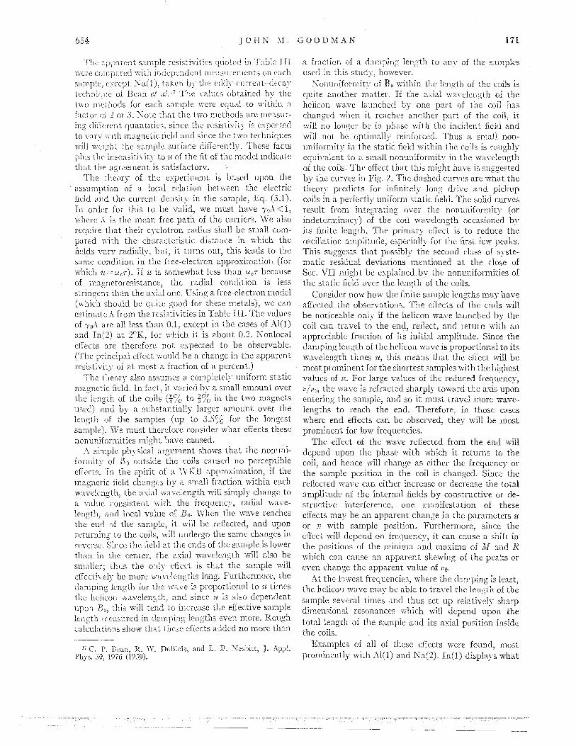
a fraction of a damping length to any of the samplesused in this study, however .Nonuniformity of B o within the length of the coils is

quite another matter . If the axial wavelength of thehelicon wave launched by one part of the coil haschanged when it reaches another part of the coil, itwill no longer be in phase with the incident field andwill not be optimally reinforced. Thus a, small non-uniformity in the static field within the coils is roughlyequivalent to a small nonuniformity in the wavelengthof the coils . The effect that this might have is suggestedby the curves in Fig . 2. The dashed curves are what thetheory predicts for infinitely long drive and pickupcoils in a perfectly uniform: static field . The solid curvesresult from integrating over the nonuniformity (orindeterminacy) of the coil wavelength occasioned byits finite length . The primary effect is to reduce theoscillation amplitude, especially for the first few peaks .This suggests that possibly the second class of syste-matic residual deviations mentioned at the close ofSec. VII might be explained by the nonuniformities ofthe static field over the length of the coils .

Consider now how the finite sample lengths may haveaffected the observations . The effects of the ends willbe noticeable only if the helicon wave launched by thecoil can travel to the end, reflect, and return with anappreciable fraction of its initial amplitude . Since thedamping length of the helicon wave is proportional to itswavelength times u, this means that the effect will bemost prominent for the shortest samples with the highestvalues of u . For large values of the reduced frequency,v/vo, the wave is refracted sharply toward the axis uponentering the sample, and so it must travel more wave-lengths to reach the end . Therefore, in those caseswhere end effects can be observed, they will be mostprominent for low frequencies .

The effect of the wave reflected from the end willdepend upon the phase with which it returns to thecoil, and hence will change as either the frequency orthe sample position in the coil is changed . Since thereflected wave can either increase or decrease the totalamplitude of the internal fields by constructive or de-structive interference, one manifestation of theseeffects may be an apparent change in the parameters uor x with sample position . Furthermore, since theeffect will depend on frequency, it can cause a shift inthe positions of the minima and maxima of 1111 and Rwhich can cause an . apparent skewing of the peaks oreven change the apparent value of so .

At the lowest frequencies, where the damping is least,the helicon wave may be able to travel the length of thesample several times and thus set up relatively sharpdimensional resonances which will depend upon thetotal length of the sample and its axial position insidethe coils .

Examples of all of these effects were found, mostprominently with Al(1) and Na(2) . In(1) displays what

171 HALL COEFFICIENTS OF Al,

, Na, AND K

6 55

may be similar distortions, while Na(1) and Na(3), theonly other short samples, were relatively free of them .These observations are consistent with the remarksabove, since Al(1) was the shortest sample and had oneof the highest values of u, and Na(2) had a similarlyhigh u. Although In(1) and Na(1) were about the samelength as Na(2), the value of u for In(l) was less thanthat for Na(2), and u for Na(1) was lower still . Na(3)was the only short sample with the smaller diameter .The smaller diameter greatly reduced the values of Mand R; distortions in them were apparently reducedeven more .

In all cases in which changes in the axial position ofthe sample caused observable variations in Yr and R,they were periodic and had a period equal to one-halfof the wavelength of the coils, in agreement with thearguments presented above .The maximum variation in the apparent scale fre-

quency was about ±1% for Na(2), about one-half asgreat for Al(l), and inappreciable for all of the othersamples .

One consequence of these explanations of the last twocategories of systematic residuals is that one cannotexpect the "best" values of u to be very reliable . Thevariation in B o over the length of the coils will lead tochoosing too low a value of u, while the possible sharpdimensional resonances and the over-all change in theamplitudes of M and R will lead to choosing too high avalue.

The only class of systematic deviations between thetheory and the observations remaining to be explainedis the sloping baseline . This, it appears, may have beencaused by applying incorrect "corrections" to theoriginal data. As was explained in Sec . IV, data weretaken on the variation of M and R with field and fre-quency for the empty coil . These variations were causedby stray capacitance in the bridge circuit and by eddycurrents in the magnet . The observed variations weretreated as corrections and were simply subtracted fromthe original data before any analysis was attempted .Certainly this is appropriate for that part of the effectcaused by stray capacitance in the bridge circuit, but thecase is not so clear for that portion caused by eddycurrents . The wave fields external to the coils whichcause the eddy currents will be modified by the presenceof a sample, and so this part of the "corrections" shouldbe modified in some nonobvious way . Changing thecorrections used by a modest fraction could in all casesremove the observed sloping baseline . It appears thatthis is the most likely explanation of this effect .

If these explanations can be accepted, one can saythat all of the observations are quantitatively explainedby the model with suitable parameter values, makingreasonable allowance for those aspects of the experimentthat did not quite conform to the assumptions of thetheory. All of the parameter values obtained in thefitting of the theory to the observations except v o have

been discussed and found to be within the experimentaluncertainties of their expectedd values .

The ratios in Table IV are, in each case, the ratio ofthe experimentally best scale frequency to the a prioriv o . The experimental value was determined by examin-ation of graphs such as Figs . 7 and 3. The scale fre-quency was chosen for best agreement with the observedperiodicity in 111 and R . The value of the standard errorachieved was used as a guide but not as the determiningcriterion, since its indication could be biased by thesystematic residuals described at the close of Sec . VII .The a priori scale frequencies were calculated from thevalues of (Ne) -'i in Table II, the value of B o, and thevalue of 'yo in Eq. (4.1), using Eq . (3 .2) . The uncer-tainties given in Table IV indicate only the accuracywith which the Pest experimental scale frequency couldbe determined . Uncertainties in the values of B„ andyo could account for any systematic deviation of allof the entries of up to 3%, but would have no influenceon the relative values . Similarly, the uncertainty in(Ne)-1 quoted in Table II may explain some of thedeviation of all of the ratios for one material fromunity, but again would not affect the spread in valuesfor that material .

The first conclusion that one can draw from the datain Table IV is that for each material the ratios are con-sistent. This conclusion justifies calculating a value forthe experimental flail coefficient of each of the materialsfrom a weighted mean of these ratios. These experi-mental Hall coefficients are listed in Table II . The un-certainties quoted there include an allowance for theuncertainties in Bo, -y o, and y, as well as the uncer-tainties in the weighted means of the ratios in Table IV .

With the exception of sodium, the experimental Hallcoefficients of all of the materials are very close to thetheoretical values, indeed, closer than the quoted un-certainties would lead one to expect . This makes therelatively large deviations from unity of the ratios inTable IV for Na(1), Na(3), and na,(4) and the defi-nitely smaller deviations for Na(5) seem likely to besignificant .

One possible clue to understanding this anomaly isthe fact that of the materials studied, only sodiumundergoes a martensitic phase transformation at lowtemperatures. Barrett' 2 claimed that the densities inthe two phases were equal to within his experimentalaccuracy, and so one would not expect the transforma-tion to alter the Hall coefficient perceptibly . But sinceit is known that the phase change alters the intrinsicresistivity of sodium," perhaps this point should bestudied in greater detail .

It must be pointed out that since the uncertaintiesin the experimental Hall coefficients R1, quoted inTable II are riot much larger than those quoted for(l'e) i, no great improvement in the test of their

18J. S . Dugdale and B . Gugan, Proc. Roy. Soc . (London)A254, 184 (1960) .

equality can be expected simply from improvements inthe experiments reported here . if one does desire tomeasure IJ.all coefficients to higher accuracy by , thistechnique, one should arrange to use very much longersamples and a much more uniform static magnetic field(att least over the region of the coils) . It would also bedesirable to make a precise determination of the coilradii at helium temperature by some direct technique,since their values (together with the coil wavelength)are needed for the most precise determination of R 11.In order to use improved Hall measurements either asa test of the theory of metals or to search for magneticbreakdown in materials with presumably closed Fermisurfaces, one must have comparably accurate data onthe number density of the atoms in the sample . Thismeans that one should be prepared, especially forsodium, to take both Hall and x-ray measurements onthe same sample without warming it in between .

IX. SUMMARY

The theory developed in this paper, followingLegendy's prescription for dealing with helicon-wave-boundary-value problems, quantitatively describes theobservations on the inductance and resistance of aspecial coil system surrounding a cylindrical metalsample parallel to a large static magnetic field . Inparticular, the large power dissipation which dependsonly weakly on the sample material's resistivity andwhich was a key prediction of Legendy's has beenobserved, and all of the predicted properties have beenverified quantitatively. This validates his approach and,in particular, his suggested boundary condition thecontinuity of all components of the wave magneticfield at the sample surface-without which the largepower loss would not have occurred .

The Hall coefficients of aluminum, indium, sodium,and potassium have been measured and shown to beequal to their theoretical high-field values to within anexperimental accuracy of about 1/2%, although the datasuggest that there may be a small discrepancy for

sodium. The theoretical values were calculated byassuming one electron per sodium or potassium atomand one hole per atom of indium or aluminum, althoughthe signs of the Hall coefficients were not checked inthis experiment .

ACKNOWLEDGMENTS

The work described in this paper benefited greatlyfrom the generous and expert assistance of manypersons, of whom only a few can be mentioned here .

This investigation has built directly upon the theoreticalwork of Charles Legendy, who also contributed tosome of the early experimental work . Dr. Raymond

Bowers and Dr . Bruce Maxfield were constant sourcesof encouragement and helpful advice, as were all of

Similarly, we must describe the Fourier components ofthe source of the fields, the primary-coil current density .It is useful to write this current density as a product ofthe current A coswt and the "winding density" of thecoil n,(r) . The winding densities of the two coils are

where the resistivity p and Hall coefficient R11 areassumed to be scalar quantities and independent ofposition within the sample. This relation is what Eq .(3.1) becomes when it is linearized by neglect of thewave field b . In combining Eq. (Al) with Maxwell'sequations, we shall neglect displacement currents .

It is convenient to consider Fourier components ofthe wave fields of the form b(r) exp(i(vi+n p--yz)} .The cylindrical symmetry permits consideration ofonly the n=0 terns . The amplitude b,,,, (r) is defined by

the members of our research group . Frank Gombasprovided the necessary expert machining, Sidney Tall-man gave much skillful technical assistance of manykinds, and James Garland assisted with the measure-ments. Dr. Watt W. Webb made available his high-uniformity superconducting solenoid . Dr. Brian K .Jones is to be thanked for several helpful discussions .

APPENDIX : DERIVATION OFTHEORETICAL MODEL

In this section, the exact expressions for the expectedvalues of the mutual inductance It and mutual resis-tance R are derived . The geometry assumed is indicatedin Fig . 1. Starting from a primary-coil drive currentA cost., the magnetic field everywhere is calculated .Then the secondary-coil voltage is calculated from thetune rate of change c the flux linking it . Finally, usingEq. (2 .1), the results are expressed in terms of 37 and R .

We shall write vector quantities in any one of threeforms interchangeably : bold face type, e .g ., B ; a scalartimes a unit vector, e .g ., Bo ^z ; or in component formenclosed in parentheses, e .g., (BT,B,,B,) . Whenevercomponents are used, they will be referred to a cylin-drical coordinate system with the z axis along the staticmagnetic field at the center of the sample and coilsystem .

The total magnetic field (r,1.) can be written as thesum of the static field Boz and the wave field b(r,t) .Inside the metal the electric field E(r,t) and the currentdensity j(r,t) are assumed to be related by

656

JOHN M . GOODMAN

171

where .I (x) is the Vessel function of the first kind oforder n, and and 1~ (x) are the modified Besselfunctions of the first and second kinds .i 9

and Ko'zr ,

Thesedefinitions were reversed in t cr . 4 .

where bz(r,t) is the z component of the total wave field .Since the radius of the secondary coil P is greater thanthat of the primary d, it is convenient to change thelower limit on the r integration from zero to infinity,This is permissible because the flux lines of the wavefield are closed . Using this form, the integration is onlyover region I, and so only C 1 land hence ,~ t) need beevaluated .

For smite values of u (i .e ., p ~z 0), the function F, andhence the f> „ can be evaluated only numerically .

The flux linking the secondary coil is

The form of the fields in region III has been given byLegendy. 4 The magnetic-field amplitudes are given by

There are three regions to consider when calculatingthe wave fields : Region I is the vacuum outside the coil(r> d), region II is the vacuum inside the coil (d> r> a),and region III is the interior of the sample (0<r<a) .Since we are neglecting displacement currents, thesolutions in regions I and II are magnetostatic fieldsand must vanish as r >co . The other boundary con-ditions on the Fourier-component amplitudes are

where g='y/yo and 0<s<' . The coil has wavelength Xand consists of 20 sections, each sX long and containingN turns. The nominal coil wave number is y o and equals27r/A . The quantity -X 2(y) is plotted in Fig . 4(b) .

We may now write the primary-coil current density as

A change in the sign of a-, at most changes the sign ofthe corresponding coefficient C4 or C 5 .

The solutions for the five coefficients are as follows :

where &(x) is the Dirac & function . The linear windingdensity (in turns/meter) A() is the same for both coilsand is plotted in Fig . 4(a) . Its Fourier transform X(,) isdefined by

The quantities s a_ and a, are defined in terms of thesample properties by

I_7I.

HALL COEFFICIENTS OF At, In, Na, AND K

d.5

653

D Al A N,

IM

it can readily be show that 11 and Q are real functions .Combining this wi', h Eqs. (A2) . (A4), (A-j), (A9), and(AII) and ni,-Ikin; use of the fact that is an oddfunction,

get the follown.g, forniulas for -If and R :

where f,5 and fA , defined by (AIO), (A12) ; (A13),and (A15), L~C functions of the frequency , (- 12v)amd the parameter arguments gx, gy , u , and fvIneither of the linmit5 a 0 (and hence a -> 0) or Pf. --+ 0,fS tends to unity and tends to zero . Thus Eq . (A.17)evaluated with 3=1 gives the theoretical of theno sample inductance Ff 0 .

Writing inserting q . Sat) 3A using 11; (3.l), w have,Analy,