softcon: simulation and control of soft-bodied animals

SoftCon: Simulation and Control of Soft-Bodied Animals withBiomimetic Actuators

SEHEE MIN, Seoul National UniversityJUNGDAMWON, Seoul National UniversitySEUNGHWAN LEE, Seoul National UniversityJUNGNAM PARK, Seoul National UniversityJEHEE LEE, Seoul National University

Fig. 1. The octopus swims by actuating muscles embedded in the soft tissues.

We present a novel and general framework for the design and control ofunderwater soft-bodied animals. The whole body of an animal consistingof soft tissues is modeled by tetrahedral and triangular FEM meshes. Thecontraction of muscles embedded in the soft tissues actuates the body andlimbs to move. We present a novel muscle excitation model that mimics theanatomy of muscular hydrostats and their muscle excitation patterns. Ourdeep reinforcement learning algorithm equipped with the muscle excita-tion model successfully learned the control policy of soft-bodied animals,which can be physically simulated in real-time, controlled interactively, andresilient to external perturbations. We demonstrate the effectiveness of ourapproach with various simulated animals including octopuses, lampreys,starfishes, stingrays and cuttlefishes. They learn diverse behaviors suchas swimming, grasping, and escaping from a bottle. We also implementeda simple user interface system that allows the user to easily create theircreatures.

CCS Concepts: • Computing methodologies→ Animation; Physical sim-ulation; Reinforcement learning; Volumetric models.

Additional Key Words and Phrases: character animation, deformable charac-ter, soft-bodied animal, finite elementmethod, physics-based control, optimalcontrol, reinforcement learning

Authors’ addresses: Sehee Min, Department of Computer Science and Engineering,Seoul National University, [email protected]; Jungdam Won, Department of Com-puter Science and Engineering, Seoul National University, [email protected]; Seungh-wan Lee, Department of Computer Science and Engineering, Seoul National University,[email protected]; Jungnam Park, Department of Computer Science and Engi-neering, Seoul National University, [email protected]; Jehee Lee, Departmentof Computer Science and Engineering, Seoul National University, [email protected].

© 2019 Association for Computing Machinery.This is the author’s version of the work. It is posted here for your personal use. Not forredistribution. The definitive Version of Record was published in ACM Transactions onGraphics, https://doi.org/10.1145/3355089.3356497.

ACM Reference Format:Sehee Min, Jungdam Won, Seunghwan Lee, Jungnam Park, and Jehee Lee.2019. SoftCon: Simulation andControl of Soft-BodiedAnimalswith BiomimeticActuators. ACM Trans. Graph. 38, 6, Article 208 (November 2019), 12 pages.https://doi.org/10.1145/3355089.3356497

1 INTRODUCTIONSoft-bodied animals are common types of animals on Earth. Mostsoft-bodied animals on the ground are small (e.g., worms) becausethey do not have internal supporting structures that help them re-sist gravity, whereas soft-bodied animals under the water can growbigger (e.g., giant squids). Soft-bodied animals lack hard parts, suchas skeletons and shells, and their bodies are mainly composed offleshes and muscles. There have been a series of studies in biol-ogy as to how soft-bodied animals, such as octopuses and squids,move their bodies and perform all the functions that are usuallyperformed by skeletons in vertebrates [Yekutieli et al. 2003]. Soft-bodied manipulators, such as octopus arms, elephant trunks, andvertebrate tongues, are called muscular hydrostats. Compared toarticulated arms, muscular hydrostats are hyper-redundant manipu-lators having a large number of degrees of freedom. For example,the octopus arm has long muscle fibers along the entire length ofthe arm, and every single segment can be activated independentlyto have a continuum of controllable muscle fibers.

The passive simulation of deformable objects has long been an ac-tive research topic in computer graphics and employed in film mak-ing, in game development, and even in material science for simulat-ing various material and relevant physical phenomena [Smith et al.2018]. However, there have been only a few studies on active simula-tion of deformable soft-bodied animals and their control. There areseveral technical challenges in creating interactively controllablesoft-bodied creatures. The challenges include the physics-based

ACM Trans. Graph., Vol. 38, No. 6, Article 208. Publication date: November 2019.

208:2 • Min et. al

modeling and simulation of soft tissues, muscles, and their contrac-tion dynamics, the robust control of highly redundant dynamicssystems, and mimicking the biological motion of live creatures.In this paper, we present a novel and general framework for the

design and control of soft-bodied animals. We are particularly in-terested in underwater animals with a variety of body shapes andactuation structures. The soft tissues and muscles are modeled bytetrahedral Finite Element Method (FEM) meshes. Nerve cords de-liver excitation signals to cause muscle contraction. We developeda new muscle excitation model, which we call Adaptive PropagationMuscle Excitation Model (AP-MEM). Our model is biomimetic in thesense that it mimics the way muscle excitation signals propagatealong muscular hydrostats. The new muscle excitation model isa key component that allows us to reproduce swimming patternsthat resemble those of real creatures. We incorporated the muscleexcitation model into a Deep Reinforcement Learning (DRL) algo-rithm to construct the controllers of soft-bodied animals, which canbe physically simulated in real-time, controlled interactively, andresilient to an external perturbation such as collisions.We will demonstrate various simulated animals including lam-

preys, starfishes, octopuses, stingrays, and cuttlefishes. The simu-lated animals learned to swim and perform goal-driven (task-based)maneuvers. We also developed a simple user interface system thatallows the user to easily create their creatures.

2 RELATED WORKPhysically Simulated Characters. The research on physically sim-

ulated characters has pursued improving physical realism, respon-siveness to the user’s control, and robustness against external per-turbation. Although human-like bipeds have been at the center ofinterests for decades [Coros et al. 2010; da Silva et al. 2008; Hodginset al. 1995; Laszlo et al. 1996; Lee et al. 2018, 2014; Liu et al. 2016;Sok et al. 2007; Wang et al. 2012; Ye and Liu 2010; Yin et al. 2007],quadruped [Coros et al. 2011], multi-legged [Fang et al. 2013], swim-ming [Grzeszczuk et al. 1998; Pan and Manocha 2018; Tan et al. 2011;Tu and Terzopoulos 1994], flying [Ju et al. 2013; Pan and Manocha2018; Wu and Popović 2003], and even imaginary creatures [Coroset al. 2012; Tan et al. 2012] have also been studied and demonstrated.Recently, DRL has gained great attention in physics-based charactercontrol due to its powerful capability of learning controllers [Liuand Hodgins 2018; Peng et al. 2018a, 2016, 2017, 2018b; Won et al.2017, 2018; Yu et al. 2018]. It has been reported that DRL is adeptat dealing with high-dimensional state and action spaces withoutselecting hand-crafted features. Since the dynamic states of soft-bodied animals and their continuum muscle fibers are inherentlyhigh-dimensional, DRL suits well for learning the control policiesof soft-bodied animals.

Passive Simulation of Deformable Objects. The passive simulationof deformable objects (e.g., clothes, hairs, rubbers, or muscles) haslong been an important research topic in computer graphics. Solv-ing the equation of motion based on implicit integration has beenregarded as a de facto method that achieves the stability and effi-ciency in deformable object simulation. Baraff and Witkin [1998]presented a fast simulation technique for mass-spring cloth modelsby solving the implicit formulation of the dynamics system, where

the potential energy induced by springs is approximated by Tay-lor series expansion. Muller et al. [2007] reproduced the physicalphenomena of various objects only in the domain of their positions,which is called position-based dynamics. Martin et al. [2011] showedthat solving the equation of motion by implicit integration can berewritten as a non-convex optimization of the potential energy,which leads to an example-based simulation by constructing poten-tial energies from examples. Bouaziz et al. [2014] proposed projectivedynamics, which introduces auxiliary projection variables to solvethe non-convex optimization formulation more efficiently. It hasbeen reported that projective dynamics substantially improves thestability and efficiency of deformable object simulation. Recently,Brandt and his colleagues [2018] developed a model reduction tech-nique for projective dynamics, which enables real-time simulationof large-scale deformable meshes. We adopted projective dynamicsas a basic simulation method for our soft-bodied animals.

Active Deformable Character Control. Althoughmost of the physics-based characters have been skeleton-driven in computer animation,deformable characters have also been studied based on optimalcontrol theory. Coping with high-dimensionality of deformableobjects is a key technical challenge and several approaches havebeen explored to circumvent the dimensionality issue. A straightfor-ward approach is to embed a skeleton into soft deformable tissuesin such a way that the character is directly driven by the skele-ton [Kim and Pollard 2011; Liu et al. 2013]. Alternatively, modelreduction techniques have been studied to reduce the dimension-ality and computational complexity of the dynamics model explic-itly [Barbič et al. 2009; Barbič and Popović 2008; Fan et al. 2014;Pan and Manocha 2018; Schulz et al. 2014]. The two-dimensionaldeformable object simulation and contractile elements were usedto animate plushies [Bern et al. 2017]. Coros et al. [2012] used thechange of rest shapes to control soft deformable characters, whichwas done by cage-based or example-based adaption. Ijiri et al. [2009]animated jellyfishes using procedural deformation. Propagation ofsignal is considered a source of character control as in our work.The difference comes from how the contraction of the soft-body isdefined. They designed a linear transformation of the local orienta-tion field for the soft-body contraction. Linear force actuators playa role in our method. Tan et al. [2012] formulated the muscle-drivencontrol of soft deformable bodies into Quadratic Programming (QP)with complementary constraints. They embedded line muscle seg-ments into soft tissues to move the body. Our simulated animals alsouse muscles as base actuators. The key difference is that our novelmuscle excitation model imitates soft-bodied animals in nature. Fur-thermore, the use of DRL makes substantial improvements overQP-based trajectory optimization in such a way that our animalsare simulated in real-time and controlled interactively.

Muscles in Soft-bodied Animals. Muscles are the only source ofactuation for the animals in nature. The contraction dynamics ofmuscles produces different actuation patterns from artificial actua-tors such as motors. The skeletal animation driven by muscles arewell-understood in computer graphics [Geijtenbeek et al. 2013; Leeet al. 2018, 2014; Wang et al. 2012]. Skeletal muscles in vertebrae areattached to bones and the functional role of each individual muscleis clearly defined by the attachment sites and its route between


SoftCon: Simulation and Control of Soft-Bodied Animals with Biomimetic Actuators • 208:3

them. Muscles of soft-bodied animals in nature are quite differ-ent. For example, the octopus arm is densely packed with musclefibers arranged in three different groups (longitudinal, transverse,and oblique) and the axial nerve cord runs along the center of thearm [Laschi et al. 2012]. The central motor signal originating fromthe brain runs down the nerve cord to activate muscle fibers sequen-tially from central to peripheral. Unlike vertebrates, for which allmotor signals originate from the brain and spinal nerves, octopusarms can move even after the arms are cut off from the body. Thisobservation implies that motor signals may originate in the nervecords along the arm. The harmony of motor signals propagatedfrom central and originated from peripheral produces distinctivewriggling movements of soft-bodied animals.

3 ANIMAL DESIGNWe assume the soft flesh is hyperelastic and use the Finite ElementMethod (FEM) to simulate the soft flesh and muscle fibers. Assumingn discrete vertices on themesh, its dynamic states can be representedby the positions of all vertices q ∈ R3n , and their velocities v ∈ R3n .A discrete-time dynamics system with implicit Euler integrationupdates positions and velocities as follows:

qt+1 = qt + hvt+1 (1)vt+1 = vt + hM−1(fint(qt+1) + fext) (2)

whereh is the time-step size,M ∈ R3n×3n is a massmatrix, fint(qt+1)= −∇E(qt+1) = −∇

∑i ViΨi (qt+1) is an internal force computed

from the summation of all element-wise elastic strain energy densi-tiesV and corresponding volumes Ψ, and fext is an external forcesuch as hydrodynamic and buoyant force. With implicit Euler in-tegration, both internal force and external force may depend onvelocities vt+1 at the next time step as well as positions qt+1. Inour case, the hydrodynamics force is supposed to be a function ofnodal velocities. We use a mixed implicit-explicit method to sim-plify the formulation such that both internal and external forces arefunctions of time t and t + 1 . The drawback of this simplification isthe potential instability of the dynamics system that requires theuse of smaller time steps. Our formulation of the hydrodynamicscircumvents the instability issue to a certain degree since drag forcemodeling viscous damping of water prevents excessively large hy-drodynamics force. Even with larger time steps, the use of constantsystem matrices derived from Projective Dynamics [Bouaziz et al.2014] achieves better computational performance than the standardFEM simulation with implicit Euler integration.

Projective Dynamics. Webriefly overview the key idea of projectivedynamics. Putting the equation (1) into equation (2) results in asystem of linear equation:[

M − h2∂f∂q

]vt+1 = Mvt + h(fint(qt ) + fext) (3)

with Taylor expansion of fint(qt+1) ≃ fint(qt ) + ∂f∂q (qt+1 − qt ) and

the Hessian ∂f∂q of E evaluated at q = qt . Once vt+1 is computed

by solving the linear system, the positions qt+1 can be computedfrom equation (1). Typical remediation of Taylor approximationalternates iteratively between solving the linear system and lineariz-ing the forces during the time step [t , t + 1], requiring the inverse

of the non-constant matrix and evaluating the Hessian at everyiteration. Alternatively, we adopt projective dynamics which pro-vides an efficient and robust solver for the equivalent problem. Thesolver divides the problem into parallelizable local solvers followedby a global quadratic problem. Let Ci be Constraint Manifold onwhich the elastic energy density function Ψi vanishes. The localminimization problem is formulated as

Ψi (q) = minpi ∈Ci

k

2∥Aiq − pi ∥2 (4)

where k is stiffness, Ai is a metric for the constraint, and pi is theprojection on manifold Ci of the current measure Aiq. The form ofCi and Ai depends on the choice of the energy model, which will bedescribed in Section 3.1. Depending on the shape of the constraintmanifold, the local problem can be non-linear and computationallyexpensive to find the projection pi . Fortunately, once projectionsare all determined at local steps, the global step can be very efficientbecause the system matrix of equation (3) is constant. Rearrangingthe equation (3) results in:

(M + h2L)qt+1 = M(qt + hvt + h2M−1fext) + Jz (5)

where L =∑i AT

i Ai , J =∑i AT

i Si , z =∑i STi pi , and Si are selector

matrices, such that pi = Si z. We factorize the matrix using theCholesky decomposition in a pre-processing step.

Hydrodynamics. We use a simplified model of hydrodynamics tosimulate the interaction between the character and the water. Thesimplified model computes drag and thrust forces on the surface ofthe mesh. The drag force approximates viscous damping of waterand acts in the direction of the relative velocity to the water. Thethrust force is a source of locomotion and acts in the opposite ofthe surface normal [Tu and Terzopoulos 1994].

fdrag = 12ρACd (Φ)∥vrel∥2d,

fthrust = − 12ρACt (Φ)∥vrel∥2n, (6)

where A is the area of the surface triangle, ρ is the density of fluid,which is approximately 1000kд/m3 for water, vrel = vwater − 1

3 (v0 +v1 + v2) is the surface velocity relative to the fluid (See figure 2).We omit the index of the surface for simplification. d = vrel

∥vrel ∥and

n are the direction of the surface velocity and the surface normal,respectively.Cd (Φ) andCt (Φ) are coefficients, which depend on theangle of attack Φ = π

2 − cos−1(n · vrel). The coefficient plot of thedrag force is symmetric, while the coefficient plot of the thrust forceis asymmetric. We lump all the drag and thrust forces on the surfaceinto a single vector fext = fhydro.

3.1 Muscular Hydrostat AnatomyThe core of the FEM simulation is designing material property. Sim-ulating muscular hydrostats requires appropriate material modelsaccording to their functional roles. The background elasticity is afundamental component that preserves the original shape as closeas possible. This elasticity is passive and independent of muscleexcitation. On top of background elasticity, the contraction andrelaxation of muscle fibers generate internal force.


208:4 • Min et. al

Fig. 2. Simplified Hydrodynamics. (Left) The drag and thrust forces. (Right) The triangles on the curved surface of the swimming stingray are colored by theangle of attack.

Background Elasticity. We choose a corotational elastic strainenergy model for background elasticity.

Ψpassive(F) =kp

2∥F − R∥2 (7)

where F = UΣV⊤ is the deformation gradient of the element, andR = UV⊤ is rotational part of the deformation gradient. In theformulation of projective dynamics, Ai maps the nodal position q tothe deformation gradient F, and pi ∈ SO(3) is the projection of thedeformation gradient onto the rigid transformation of the rest shape.The element-wise volume preservation energy model projects thedeformation gradient to the manifold

{D ∈ R3×3 | det(D) = 1

}.

Ψvolume(F) =kv2∥F − D∥2 (8)

where D = UΣ∗V⊤, and det(Σ∗) = 1. We find D using constrainedquadratic programming.We refer to the work of Bouaziz et al. [2014]for the details on the relevant algebra.

Muscle fibers and cords. The anatomy of the soft-bodied arm com-prises several muscle groups with numerous muscle fibers. Physio-logically, muscles contract and relax along the direction of musclefibers. We approximate a continuum of aligned muscle fibers byFEM mesh elements (either tetrahedrons or triangles) and a nervecord. The muscle excitation signal u travels through the nerve cord,which is discretized into a sequence of segments ui , and activatesnearby FEM elements within a user-specified radius. (See Figure 3)The activated element contracts along the direction of the nearestcord segment. The level of activation of element e is inversely pro-portional to the distance to the cord l , which can be formulated ase = uiexp(−σl). The contraction of an FEM element generates inter-nal force fmuscle(e) = −∇Emuscle, where Emuscle is a muscle energymodel, which depends on the type of muscle fibers. We considertwo types, contractile and bending. The muscle excitation model willbe discussed in the next section.

Contractile fibers. The contractile muscle generates anisotropicmuscle force fmuscle(e) = −fmuscle(e)m where m is the muscle fiberdirection. To generate such an anisotropic muscle force fmuscle(e),we adopt a strain energy model Emuscle = VmuscleΨmuscle [Lee et al.2018].

Ψmuscle(F, e) =km2

∥(1 − r )Fm∥2 (9)

Fig. 3. The nerve cord delivers muscle excitation signal u through musclefibers approximated by FEM elements. The activated elements are shownin red.

where km is muscle stiffness, e ∈ [0, 1] is the level of activation,r = (1 − e)/l is the projection of the cord segment. The energymodel results in linear force fmuscle(e) = −k(l − (1 − e)) with amuscle stretch factor l = ∥Fm∥. From the viewpoint of projectivedynamics, r is the projection of the contraction axis given activatione . The global solver balances background elasticity and contractilemuscle forces by solving a quadratic optimization problem.

Bending Fibers. Some of the underwater soft-bodied animals havethin body parts such as fins. The whole body of some underwateranimals is too thin to model with tetrahedral meshes. Simulatingsuch thin structures with tetrahedral meshes could suffer from aninstability issue stemming from the material-space singularity. In-stead, we rather utilize a thin-shell model that is actuated by bendingmuscles. In nature, all muscles produce force by contraction. Weconsider an imaginary type of muscles that produce force by bend-ing. Bending muscles take a signed excitation signal and the signindicates the direction of bending. Simulating two-dimensional thin-shells in three-dimensional space requires an energy term on thebending phenomenon. We follow the one-ring bending energy pro-posed by [Nealen et al. 2006], which uses isotropic deformationrepresented by the Laplace-Beltrami operator for each edge.

Ψbending(q0, q1, q2, q3, e) =kb2∥Xc − RX̃(e)c∥2 (10)



where q0 and q1 are vertices constituting an edge and q2 and q3are its adjacent vertices. X = (q0, q1, q2, q3) ∈ R3×4 is the currentposition matrix, X̃(e) is the rest position matrix deformed by acti-vation e ∈ [−1, 1], and c is a set of cotangent weights for the edge.R ∈ SO(3) is a projection such that rotating X̃(e)c by R best matchesto X(q)c. We detail on how activation e updates the rest shape inthe Appendix.

3.2 Muscle Excitation ModelWe can consider several different models for muscle excitation. Thesimplest model assumes that all excitation signals on the segmentsare independent. We call it Independent Muscle Excitation Model(I-MEM). Although I-MEM allows for maximal flexibility in move-ments and provides the largest degrees of freedom in control, thehigh-dimensionality of control is a big obstacle for learning motorskills. The direct opposite model to I-MEM assumes that all segmentson the entire length of the nerve cord share the same excitationsignal. We call it Shared Muscle Excitation Model (S-MEM). Thoughthis model coordinates muscle movements in a structured manner,the model is too simple to reproduce complex behaviors. An alter-native to these two extremes is a Central Pattern Generator model(CPG-MEM), which produces cyclic excitation signals from the cen-tral nervous system and propagates the signal to peripherals. Thismodel has been popular in computer graphics and robotics becauseit produces wiggling patterns that look biological [Si et al. 2014; Tianand Lu 2015]. In this model, the central nervous system takes fullcontrol over the movements and it modulates the central patterns tochange the direction and speed in a strongly-structure manner. Wepresent a new biomimetic muscle excitation model, which we callAdaptive Propagation Muscle Excitation Model (AP-MEM), inspiredby signal delivery in muscular hydrostats.

Our model is based on two key observations that can be found inthe biology literature. It has been observed from octopuses that ner-vous signals are produced not only at the brain but also at any partof the limb, as evidenced by amputated octopus arms. The centralnervous signals originated from the brain are actively modulated inthe peripheral [Levy and Hochner 2017; Richter et al. 2015]. Centralnerve signals act as high-level commands from the brain, and thesignals are modulated and adjusted to perform skilled control andmanipulation. It has also been noted that the speed of neural signaltransmission varies in the movement of organisms [Hochner 2012].The careful modulation of signal propagation speed is as importantas signal amplitude modulation. Our AP-MEM is a simple modelthat satisfies these observations. The AP-MEM is also equipped witha central pattern generator that produces central excitation signals,which are adapted dynamically while propagating to peripherals.

Central Pattern Generator. The various forms of cyclic patternshave been studied and exploited in the composition of center ner-vous signals. We choose the simple triangular wave function asinitial central pattern which is good enough to control all the ani-mals in our examples (see Figure 4). The triangular wave functionwith range θ2 and period t ∈ [0,θ1] is

TW (t |θ1,θ2) =θ22

[ 4θ1

(t −

θ14

−θ12

⌊ 2tθ1

⌋ )(−1)

⌊2tθ1

⌋+ 1

], (11)

Fig. 4. Triangular central nerve signals at the top propagate through nervecords when propagation parameters (α, β, κ) are constant.

where ⌊·⌋ is the floor function. If the triangular signal occurs repeat-edly at the interval θ3 ≥ θ1, the central pattern is defined by

µ(t |θ1,θ2,θ3) =

{TW (t ;θ1,θ2), if t ∈ [0,θ1]0, if t ∈ (θ1,θ3].

(12)

The presence of delay (θ3 − θ1) between excitation signals pro-duces a mixture of movement and holding as shown in energeticthrusts in octopus swimming and highly curved S-shapes of ribboneels.

Adaptive Propagation. The propagation operator delivers excita-tion signals, ui , along with nerve cord segments where i = 0, 1, · · ·indexes segments from proximal to distal. While propagating, thesignal ui is modulated spatially by parameters α and β , and tempo-rally by parameter κ when the central signal µ is given to proximalto the muscle cord.

ui (t + 1) =

{µ(t), if i = 0αui−1(t) + βui (t), otherwise,

(13)

The attenuation factor β determines how much the current levelof excitation will remain at the next time. The delivery factor αdetermines how much excitation will be propagated to the nextsegment. We repeat this step κ times at every control time step tomodulate the speed of the propagation process. The propagationoperator at time t is defined by

u(t + 1) = Pκu(t) =

0 0 0 . . . 0 µα β 0 . . . 0 00 α β . . . 0 0.......... . .

......

0 0 0 . . . α β0 0 0 . . . 0 1

κ

u1(t)u2(t)u3(t)...

uN (t)1

(14)

where P is a propagation matrix, and N is the number of the seg-ments. If the parameters α , β and κ are constant over time, our


208:6 • Min et. al

Fig. 5. Dynamics sdyn, task stask, and excitation sext states. (Left) Thepositions of selected vertices are colored in yellow and the blue arrows aretheir velocities. (Middle) The green and red arrows are the target velocity andaverage velocity of the character, respectively. (Right) The current excitationpattern is colored in pink.

model generates stationary CPG-MEM signals, whereas it modu-lates the central patterns µ(t) to control the full-body movements ifthe parameters change. Learning a CPG-MEM controller is computa-tionally demanding because the action originating at the beginningof the nerve cord can be evaluated at the end of the propagation. Theoccurrence of an action and its evaluation are distant spatially andtemporally. Our AP-MEM takes a different approach to modulatingthe propagation parameters to add flexibility and controllability inthe middle of a long muscle. We found that our AP-MEM bettersuits for policy learning in the next section.

4 CONTROLLER LEARNINGIn reinforcement learning (RL), an agent (a soft-bodied animal inour study) in state s takes action a, and its state changes to s′ withtransition probability P(s, a, s′) ∈ [0, 1]. RL assumes the Markovproperty, meaning that the transition probability depends only onthe current state. The agent receives a scalar-valued reward r =R(s, a, s′) in the transition proportional to the desirability of thetransition. The initial state s0 of the agent is chosen from initialstate probability ρ(s0). The state changes sequentially by takingactions until it meets a termination condition (e.g., time limit andfailure detection of the given task). The sum of discounted rewardscollected during this process is called a return G(s0) = r0 + γr1 +γ 2r2 + γ 3r3 + · · · , where γ ∈ [0, 1) is a discount factor that makesthe sum finite. The goal of reinforcement learning is to find a policy(a.k.a. controller) that maximizes the expected value of the returngiven the initial state distribution.The state s = (sdyn, stask, sexc) is composed of the dynamical

state, task-specific state, and the excitation state (See Figure 5). Thedynamical state sdyn = (x, Ûx) includes vertex positions x and theirvelocities Ûx of the FEM mesh. We found that it is not necessary toinclude all vertices in the state, but we randomly select k vertices(n ≫ k) near the nerve cords. The positions and velocities arerepresented in a local, moving coordinate system attached to theanimal’s body. The task state stask gives the information of user-provided goals where we use the target velocity represented inthe local coordinate system for underwater locomotion. sexc is thecurrent excitation pattern u(t). The user provides with central nervesignals µ0(t) parameterized by (θ1,θ2,θ3), and the initial values ofpropagation parameters (α0, β0,κ0) for each individual nerve cord j .The action is the modulation of the central pattern and propagation

parameters. The actual parameters at muscle j are

µ = µ0(t) + ∆µ, α = α0 + ∆α , β = β0 + ∆β , κ = κ0 + ∆κ, (15)

when action (∆µ,∆α ,∆β ,∆κ) is applied.The reward for the underwater navigation task encourages the

agent to move along the target velocity.

R = w1exp(− σ1∥vd −v ∥

)+w2exp

(− σ2∥dd − d∥2

)+w3exp

(− σ3∥θup∥

)+ rtask.

(16)

where vd = ∥vd∥ ∈ R and dd =vdvd

∈ S2, respectively, are thelength, v is the average body velocity during 1 s. and the directionof the target velocity vd ∈ R3 and θup ∈ R is the angle betweenthe up vector and the global upward direction. rtask depends on thechoice of task objectives.Our policy and value functions are deep networks with three

fully connected layers with 128 units for each layer. The internallayers use tanh units for non-linear activation and the last layeruses linear activation units. We adopt Proximal Policy Optimization(PPO) to directly minimize expected returns through stochasticgradient descent [Schulman et al. 2017].

5 EXPERIMENTAL RESULTOur implementation of the FEM simulation largely follows the tuto-rial provided by Sifakis and Barbic [2012] and the work of Bouazizet al. [2014]. For FEM mesh generation, we used TetWild [Hu et al.2018] for 3D tetrahedralization and Delaunay triangulation for thinplates. We typically generate meshes with 400 to 1000 vertices asa trade-off between computational costs and motor functionality(See Table 1). Each nerve cord is divided into 50 segments, whichprovide a lot of control freedom. The degrees of simulation freedomproportional to the number of vertices is much larger than its con-trol freedom. Muscle routings are specified by Bézier splines. Thesegments of nerve cords are assigned to tetrahedra by computingtriangle-spline intersections.

Since the whole body of our animal model is soft, the local coor-dinate system attached to the body can be noisy or wiggly underthe influence of muscle activation. We pick C ≥ 4 vertices to attachthe coordinate system as far away as possible from muscles (e.g., inthe head). The local coordinate system (Rlocal, blocal) is determinedby solving a minimization problem.

min(R,b)∈SO (3)×R3

∥X − (RX̃ + b)∥2 (17)

where X, X̃ ∈ R3×C are matrices horizontally stacking the verticesof deformed and material space positions, respectively, while activat-ing muscles by central patterns. This minimization problem can besolved analytically using singular value decomposition. Increasingthe Young’s modulus around the coordinate system is also helpfulin stabilizing the coordinate system.

Our learning algorithm is episodic. It learns a control policy frommany simulation episodes. The initial state s0 of each simulationepisode is picked randomly from the pool of states in previous



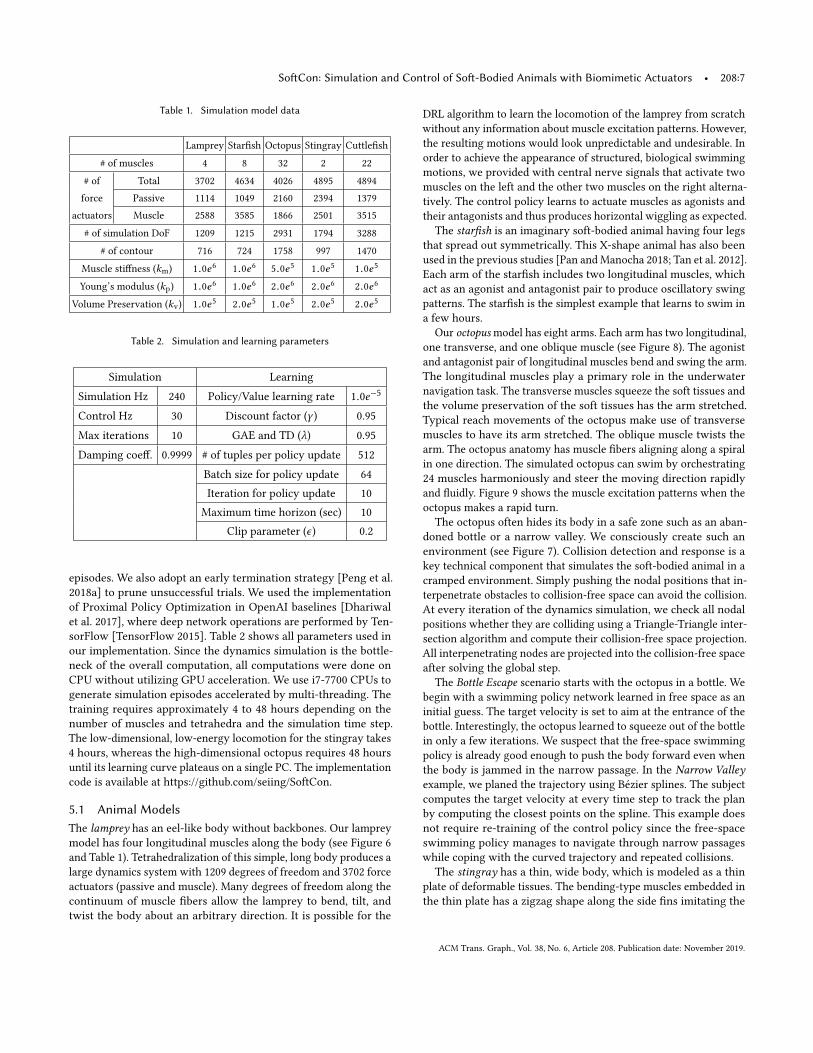
Table 1. Simulation model data

Lamprey Starfish Octopus Stingray Cuttlefish

# of muscles 4 8 32 2 22

# of Total 3702 4634 4026 4895 4894force Passive 1114 1049 2160 2394 1379

actuators Muscle 2588 3585 1866 2501 3515

# of simulation DoF 1209 1215 2931 1794 3288

# of contour 716 724 1758 997 1470

Muscle stiffness (km) 1.0e6 1.0e6 5.0e5 1.0e5 1.0e5

Young’s modulus (kp) 1.0e6 1.0e6 2.0e6 2.0e6 2.0e6

Volume Preservation (kv) 1.0e5 2.0e5 1.0e5 2.0e5 2.0e5

Table 2. Simulation and learning parameters

Simulation Learning

Simulation Hz 240 Policy/Value learning rate 1.0e−5

Control Hz 30 Discount factor (γ ) 0.95

Max iterations 10 GAE and TD (λ) 0.95

Damping coeff. 0.9999 # of tuples per policy update 512

Batch size for policy update 64Iteration for policy update 10

Maximum time horizon (sec) 10Clip parameter (ϵ) 0.2

episodes. We also adopt an early termination strategy [Peng et al.2018a] to prune unsuccessful trials. We used the implementationof Proximal Policy Optimization in OpenAI baselines [Dhariwalet al. 2017], where deep network operations are performed by Ten-sorFlow [TensorFlow 2015]. Table 2 shows all parameters used inour implementation. Since the dynamics simulation is the bottle-neck of the overall computation, all computations were done onCPU without utilizing GPU acceleration. We use i7-7700 CPUs togenerate simulation episodes accelerated by multi-threading. Thetraining requires approximately 4 to 48 hours depending on thenumber of muscles and tetrahedra and the simulation time step.The low-dimensional, low-energy locomotion for the stingray takes4 hours, whereas the high-dimensional octopus requires 48 hoursuntil its learning curve plateaus on a single PC. The implementationcode is available at https://github.com/seiing/SoftCon.

5.1 Animal ModelsThe lamprey has an eel-like body without backbones. Our lampreymodel has four longitudinal muscles along the body (see Figure 6and Table 1). Tetrahedralization of this simple, long body produces alarge dynamics system with 1209 degrees of freedom and 3702 forceactuators (passive and muscle). Many degrees of freedom along thecontinuum of muscle fibers allow the lamprey to bend, tilt, andtwist the body about an arbitrary direction. It is possible for the

DRL algorithm to learn the locomotion of the lamprey from scratchwithout any information about muscle excitation patterns. However,the resulting motions would look unpredictable and undesirable. Inorder to achieve the appearance of structured, biological swimmingmotions, we provided with central nerve signals that activate twomuscles on the left and the other two muscles on the right alterna-tively. The control policy learns to actuate muscles as agonists andtheir antagonists and thus produces horizontal wiggling as expected.

The starfish is an imaginary soft-bodied animal having four legsthat spread out symmetrically. This X-shape animal has also beenused in the previous studies [Pan andManocha 2018; Tan et al. 2012].Each arm of the starfish includes two longitudinal muscles, whichact as an agonist and antagonist pair to produce oscillatory swingpatterns. The starfish is the simplest example that learns to swim ina few hours.

Our octopusmodel has eight arms. Each arm has two longitudinal,one transverse, and one oblique muscle (see Figure 8). The agonistand antagonist pair of longitudinal muscles bend and swing the arm.The longitudinal muscles play a primary role in the underwaternavigation task. The transverse muscles squeeze the soft tissues andthe volume preservation of the soft tissues has the arm stretched.Typical reach movements of the octopus make use of transversemuscles to have its arm stretched. The oblique muscle twists thearm. The octopus anatomy has muscle fibers aligning along a spiralin one direction. The simulated octopus can swim by orchestrating24 muscles harmoniously and steer the moving direction rapidlyand fluidly. Figure 9 shows the muscle excitation patterns when theoctopus makes a rapid turn.The octopus often hides its body in a safe zone such as an aban-

doned bottle or a narrow valley. We consciously create such anenvironment (see Figure 7). Collision detection and response is akey technical component that simulates the soft-bodied animal in acramped environment. Simply pushing the nodal positions that in-terpenetrate obstacles to collision-free space can avoid the collision.At every iteration of the dynamics simulation, we check all nodalpositions whether they are colliding using a Triangle-Triangle inter-section algorithm and compute their collision-free space projection.All interpenetrating nodes are projected into the collision-free spaceafter solving the global step.

The Bottle Escape scenario starts with the octopus in a bottle. Webegin with a swimming policy network learned in free space as aninitial guess. The target velocity is set to aim at the entrance of thebottle. Interestingly, the octopus learned to squeeze out of the bottlein only a few iterations. We suspect that the free-space swimmingpolicy is already good enough to push the body forward even whenthe body is jammed in the narrow passage. In the Narrow Valleyexample, we planed the trajectory using Bézier splines. The subjectcomputes the target velocity at every time step to track the planby computing the closest points on the spline. This example doesnot require re-training of the control policy since the free-spaceswimming policy manages to navigate through narrow passageswhile coping with the curved trajectory and repeated collisions.

The stingray has a thin, wide body, which is modeled as a thinplate of deformable tissues. The bending-type muscles embedded inthe thin plate has a zigzag shape along the side fins imitating the


208:8 • Min et. al

Fig. 6. The FEM meshes and nerve cords of assorted soft-bodied animals. (From left to right) Lamprey, starfish, octopus, stingray and cuttlefish.

Fig. 7. The animals in cramped environments. (Left to Right) The octopus escaping the bottle, the octopus swimming through a narrow valley, and the ribboneels passing through obstacles.



Fig. 8. Octopus arms. The contraction of longitudinal, transverse andoblique muscles respectively bend, lengthen and twist the arm.

Fig. 9. The octopus turning. The longitudinal muscle inside the arm shownin green plays a role in making forward thrusts, while another longitudinalmuscle outside the arm shown in pink plays an opposite role in recoveringthe arm position for the next thrust and making backward thrusts to brake.The octopus makes strong thrusts with the arms outside of turning andbrakes with the arms inside to change its moving direction rapidly.

anatomy of stingrays [Park et al. 2016]. Propagating muscle excita-tion signals through the zigzag muscles produce wavy, flutteringmovements of soft fins. We also created a variety of imaginary, thin-shell animals actuated by various muscles and their embeddings.

The Cuttlefish has a volumetric body with ten short arms and thinfins on both sides of the body. It has two longitudinal contractilemuscles in each arm and a bending muscle in each fin. It can moveforward slowly by fluttering the fins. The arms can make additionalthrusts to move faster.

5.2 Comparison of Muscle Excitation ModelsWe compared the effectiveness of our AP-MEM with alternativemodels including I-MEM, S-MEM andCPG-MEM (See figure 10). Thefree-space swimming policies for the lamprey, the starfish and theoctopus are learned with different MEMs and we compared their av-erage returns and learning time. The I-MEM policies achieved highaverage returns for simple animals (the lamprey and the starfish),

AP-MEM I-MEM S-MEM CPG-MEM

Lamprey 798.98 3655.67 937.25 29.39(time) 19 350 45 47.85Starfish 1684.5 1809.34 146.43 40.22(time) 6 202 22 47.85

Octopus 1503.55 8.56 15.05 N/A(time) 47 156 57 N/A

Fig. 10. Comparison of MEMs. The average return of the free-space swim-ming task and the learning time (hours) are compared.

implying that the I-MEM policies perform well in respect to achiev-ing a task-driven goal. However, the I-MEM policies produce noisy,unstructured movements that do not appear biological. The averagereturn is probably good at measuring the performance of a policy,but certainly poor at evaluating the quality of movements. Learn-ing an I-MEM policy is slow because of its excessive degrees offreedom in control. The CPG-MEM policies produce more struc-tured, better-looking movements than the I-MEM policies. Evenwith fewer degrees of freedom, learning a CPG-MEM policy forthe octopus is much slower than learning an I-MEM policy. The


208:10 • Min et. al

CPG-MEM policy for the octopus is not robust even after two weeksof learning in our experiments. The computational cost for policylearning is not proportional to the degrees of freedom, the numberof FEM elements, and the number of muscle actuators. There arequalitative factors, such as the structural complexity of the bodyand muscles, that affect more than the numbers. Our AP-MEM poli-cies out-perform all alternatives by a large margin in regards toboth computational efficiency and the quality of movements. Theadvantages of AP-MEM is more prominent when the model is morecomplex.

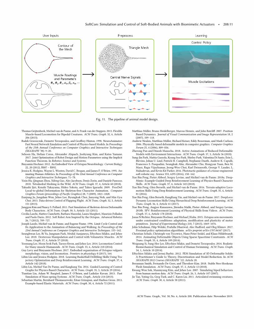
5.3 Interactive User InterfaceWe implemented a user interface system that allows the user todesign his/her own creatures easily (see Figure 11). Our user inter-face system currently supports the creation of an animal with itsthin-plate body. The interactive design of volumetric bodies is asubject for future research.The user interface system has two stages: modeling stage and

simulation stage. In the modeling stage, the user can draw the con-tour of the animal and the routes of muscles. The system generatesa triangle FEM mesh via Delaunay triangulization of the contourand embeds the nerve cords into the triangle mesh by computingthe intersection between nerve cords and triangles. In the simu-lation stage, the user specifies the initial values of central nervesignals (θ1,θ2,θ3) and propagation parameters (α0, β0,κ0) for eachmuscle, while visualizing the body deformation in simulation. Atthis stage, we disable hydrodynamic forces to focus on visualizingthe effect of central nerve signals and their propagation. Once theparameter setting is finished, the new animal model goes throughthe learning phase to learn its control policy under the influence ofhydrodynamics.

6 DISCUSSIONWe presented a framework for modeling, simulation, and controlof soft-bodied animals with biomimetic actuators. The key to thesuccess of our approach is our muscle excitation model that makes agood balance between simplicity vs. generalization capability, struc-ture vs. flexibility, and low control dimensionality vs. high modelingdimensionality. The DRL algorithm equipped with our AP-MEM cancope with the complexity of deformable soft bodies, a continuum ofmuscle fibers, and impressive numbers of DoFs and discretized mus-cle actuators. The increased dimensionality and model complexityhave been successfully translated into smooth, flexible movementsthat appear biological. We envision the framework in which accu-rate biomechanical models may be applied to truly accurate motionsfor animals alive, extinct, or imaginary.

The interactive performance of our system is largely attributed toprojective dynamics and deep reinforcement learning. The runtimesimulation on a typical desktop PC is 3 to 5 times slower than real-time if self-collision is not considered in the simulation. Collisiondetection and response are notorious computational bottlenecks ofdeformable body simulation. Although our method is much fasterthan previous systems for soft-bodied animal simulation, there isroom for performance improvements. One possibility is the im-plicit handling of hydrodynamic forces, which will lead to a full

implicit integration method that allows for larger time steps andunconditional stability.Even though successful applications of AP-MEMs have been

demonstrated so far, our framework also has numerous limitations.Underwater soft-bodied animals in nature have an alternative mech-anism to move, which we are currently unable to reproduce with thesimplified hydrodynamics model. For example, the octopus drawswater into its body cavity and spurts the water out to generate thrust.A more sophisticated hydrodynamics model, which can simulatethe incompressibility of fluids, is crucial to reproduce such behavior.Our animal models lack a lot of important anatomical features. Theoctopus has membranes between legs to push the water off and usessuckers for grabbing and holding prey. We have not implementedsuch features in our simulation model yet.The design of body shapes and the embedding of nerve cords

have significant impacts on the motor ability of the learned controlpolicy. We designed our animal models based on similar creatures innature and we often found that small tweaking of the body shapesand muscle embedding substantially affect the level of motor abil-ity and the type of motor skills the control policy can achieve. Anintriguing direction for future research is to learn the most effi-cient body shape, muscle embedding, and motion for an animalsimultaneously [Geijtenbeek et al. 2013; Ha et al. 2017].

ACKNOWLEDGMENTSThis research was supported by the MSIT(Ministry of Science andICT), Korea, under the SW Starlab support program(IITP-2017-0-00878) supervised by the IITP(Institute for Information & communi-cations Technology Promotion).

REFERENCESDavid Baraff and Andrew Witkin. 1998. Large Steps in Cloth Simulation. In Proceedings

of the 25th Annual Conference on Computer Graphics and Interactive Techniques(SIGGRAPH ’98). 43–54.

Jernej Barbič, Marco da Silva, and Jovan Popović. 2009. Deformable Object AnimationUsing Reduced Optimal Control. ACM Trans. Graph. 28, 3, Article 53 (2009).

Jernej Barbič and Jovan Popović. 2008. Real-time Control of Physically Based Simula-tions Using Gentle Forces. ACM Trans. Graph. 27, 5, Article 163 (2008).

James M. Bern, Kai-Hung Chang, and Stelian Coros. 2017. Interactive Design of Ani-mated Plushies. ACM Trans. Graph. 36, 4, Article 80 (2017).

Sofien Bouaziz, Sebastian Martin, Tiantian Liu, Ladislav Kavan, and Mark Pauly. 2014.Projective Dynamics: Fusing Constraint Projections for Fast Simulation. ACM Trans.Graph. 32, 6, Article 154 (2014).

Christopher Brandt, Elmar Eisemann, and Klaus Hildebrandt. 2018. Hyper-reducedProjective Dynamics. ACM Trans. Graph. 37, 4, Article 80 (2018).

Stelian Coros, Philippe Beaudoin, and Michiel van de Panne. 2010. Generalized BipedWalking Control. ACM Trans. Graph. 29, 4, Article 130 (2010).

Stelian Coros, Andrej Karpathy, Ben Jones, Lionel Reveret, and Michiel van de Panne.2011. Locomotion Skills for Simulated Quadrupeds. ACM Trans. Graph. 30, 4, Article59 (2011).

Stelian Coros, Sebastian Martin, Bernhard Thomaszewski, Christian Schumacher,Robert Sumner, and Markus Gross. 2012. Deformable Objects Alive! ACM Trans.Graph. 31, 4, Article 69 (2012).

Marco da Silva, Yeuhi Abe, and Jovan Popović. 2008. Interactive Simulation of StylizedHuman Locomotion. ACM Trans. Graph. 27, 3, Article 82 (2008).

Prafulla Dhariwal, Christopher Hesse, Oleg Klimov, Alex Nichol, Matthias Plappert,Alec Radford, John Schulman, Szymon Sidor, Yuhuai Wu, and Peter Zhokhov. 2017.OpenAI Baselines. https://github.com/openai/baselines. (2017).

Ye Fan, Joshua Litven, and Dinesh K. Pai. 2014. Active Volumetric MusculoskeletalSystems. ACM Trans. Graph. 33, 4, Article 152 (2014).

Jingyi Fang, Chenfanfu Jiang, and Demetri Terzopoulos. 2013. Modeling and AnimatingMyriapoda: A Real-time Kinematic/Dynamic Approach. In Proceedings of the 12thACM SIGGRAPH/Eurographics Symposium on Computer Animation (SCA ’13). 203–212.



Fig. 11. The pipeline of animal model design.

Thomas Geijtenbeek, Michiel van de Panne, and A. Frank van der Stappen. 2013. FlexibleMuscle-based Locomotion for Bipedal Creatures. ACM Trans. Graph. 32, 6, Article206 (2013).

Radek Grzeszczuk, Demetri Terzopoulos, and Geoffrey Hinton. 1998. NeuroAnimator:Fast Neural Network Emulation and Control of Physics-based Models. In Proceedingsof the 25th Annual Conference on Computer Graphics and Interactive Techniques(SIGGRAPH ’98). 9–20.

Sehoon Ha, Stelian Coros, Alexander Alspach, Joohyung Kim, and Katsu Yamane.2017. Joint Optimization of Robot Design and Motion Parameters using the ImplicitFunction Theorem. In Robotics: Science and Systems.

Binyamin Hochner. 2012. An Embodied View of Octopus Neurobiology. Current Biology22, 20 (2012), R887 – R892.

Jessica K. Hodgins, Wayne L. Wooten, David C. Brogan, and James F. O’Brien. 1995. An-imating Human Athletics. In Proceedings of the 22nd Annual Conference on ComputerGraphics and Interactive Techniques. 71–78.

Yixin Hu, Qingnan Zhou, Xifeng Gao, Alec Jacobson, Denis Zorin, and Daniele Panozzo.2018. Tetrahedral Meshing in the Wild. ACM Trans. Graph. 37, 4, Article 60 (2018).

Takashi Ijiri, Kenshi Takayama, Hideo Yokota, and Takeo Igarashi. 2009. ProcDef:Local-to-global Deformation for Skeleton-free Character Animation. ComputerGraphics Forum (proceedings of Pacific Graphics) 28, 7 (2009), 1821–1828.

Eunjung Ju, Jungdam Won, Jehee Lee, Byungkuk Choi, Junyong Noh, and Min GyuChoi. 2013. Data-driven Control of Flapping Flight. ACM Trans. Graph. 32, 5, Article151 (2013).

Junggon Kim and Nancy S. Pollard. 2011. Fast Simulation of Skeleton-driven DeformableBody Characters. ACM Trans. Graph. 30, 5, Article 121 (2011).

Cecilia Laschi, Matteo Cianchetti, Barbara Mazzolai, Laura Margheri, Maurizio Follador,and Paolo Dario. 2012. Soft Robot Arm Inspired by the Octopus. Advanced Robotics26, 7 (2012), 709–727.

Joseph Laszlo, Michiel van de Panne, and Eugene Fiume. 1996. Limit Cycle Control andIts Application to the Animation of Balancing and Walking. In Proceedings of the23rd Annual Conference on Computer Graphics and Interactive Techniques. 155–162.

Seunghwan Lee, Ri Yu, Jungnam Park, Mridul Aanjaneya, Eftychios Sifakis, and JeheeLee. 2018. Dexterous Manipulation and Control with Volumetric Muscles. ACMTrans. Graph. 37, 4, Article 57 (2018).

Yoonsang Lee, Moon Seok Park, Taesoo Kwon, and Jehee Lee. 2014. Locomotion Controlfor Many-muscle Humanoids. ACM Trans. Graph. 33, 6, Article 218 (2014).

Guy Levy and Binyamin Hochner. 2017. Embodied organization of Octopus vulgarismorphology, vision, and locomotion. Frontiers in physiology 8 (2017), 164.

Libin Liu and Jessica Hodgins. 2018. Learning Basketball Dribbling Skills Using Tra-jectory Optimization and Deep Reinforcement Learning. ACM Trans. Graph. 37, 4,Article 142 (2018).

Libin Liu, Michiel Van De Panne, and Kangkang Yin. 2016. Guided Learning of ControlGraphs for Physics-Based Characters. ACM Trans. Graph. 35, 3, Article 29 (2016).

Tiantian Liu, Adam W. Bargteil, James F. O’Brien, and Ladislav Kavan. 2013. FastSimulation of Mass-spring Systems. ACM Trans. Graph., Article 214 (2013).

Sebastian Martin, Bernhard Thomaszewski, Eitan Grinspun, and Markus Gross. 2011.Example-based Elastic Materials. ACM Trans. Graph. 30, 4, Article 72 (2011).

Matthias Müller, Bruno Heidelberger, Marcus Hennix, and John Ratcliff. 2007. PositionBased Dynamics. Journal of Visual Communication and Image Representation 18, 2(2007), 109–118.

Andrew Nealen, Matthias Müller, Richard Keiser, Eddy Boxerman, and Mark Carlson.2006. Physically based deformable models in computer graphics. Computer GraphicsForum 25, 4 (2006), 809–836.

Zherong Pan and Dinesh Manocha. 2018. Active Animations of Reduced DeformableModels with Environment Interactions. ACM Trans. Graph. 37, 3, Article 36 (2018).

Sung-Jin Park, Mattia Gazzola, Kyung Soo Park, Shirley Park, Valentina Di Santo, Erin L.Blevins, Johan U. Lind, Patrick H. Campbell, Stephanie Dauth, Andrew K. Capulli,Francesco S. Pasqualini, Seungkuk Ahn, Alexander Cho, Hongyan Yuan, Ben M.Maoz, Ragu Vijaykumar, Jeong-Woo Choi, Karl Deisseroth, George V. Lauder, L.Mahadevan, and Kevin Kit Parker. 2016. Phototactic guidance of a tissue-engineeredsoft-robotic ray. Science 353, 6295 (2016), 158–162.

Xue Bin Peng, Pieter Abbeel, Sergey Levine, and Michiel van de Panne. 2018a. Deep-Mimic: Example-Guided Deep Reinforcement Learning of Physics-Based CharacterSkills. ACM Trans. Graph. 37, 4, Article 143 (2018).

Xue Bin Peng, Glen Berseth, and Michiel van de Panne. 2016. Terrain-adaptive Loco-motion Skills Using Deep Reinforcement Learning. ACM Trans. Graph. 35, 4, Article81 (2016).

Xue Bin Peng, Glen Berseth, KangKang Yin, and Michiel van de Panne. 2017. DeepLoco:Dynamic Locomotion Skills Using Hierarchical Deep Reinforcement Learning. ACMTrans. Graph. 36, 4, Article 41 (2017).

Xue Bin Peng, Angjoo Kanazawa, Jitendra Malik, Pieter Abbeel, and Sergey Levine.2018b. SFV: Reinforcement Learning of Physical Skills from Videos. ACM Trans.Graph. 37, 6, Article 178 (2018).

Jonas N Richter, Binyamin Hochner, and Michael J Kuba. 2015. Octopus armmovementsunder constrained conditions: adaptation, modification and plasticity of motorprimitives. Journal of Experimental Biology 218, 7 (2015), 1069–1076.

John Schulman, Filip Wolski, Prafulla Dhariwal, Alec Radford, and Oleg Klimov. 2017.Proximal policy optimization algorithms. arXiv preprint arXiv:1707.06347 (2017).

Christian Schulz, Christoph von Tycowicz, Hans-Peter Seidel, and Klaus Hildebrandt.2014. Animating Deformable Objects Using Sparse Spacetime Constraints. ACMTrans. Graph. 33, 4, Article 109 (2014).

Weiguang Si, Sung-Hee Lee, Eftychios Sifakis, and Demetri Terzopoulos. 2014. RealisticBiomechanical Simulation and Control of Human Swimming. ACM Trans. Graph.34, 1, Article 10 (2014).

Eftychios Sifakis and Jernej Barbic. 2012. FEM Simulation of 3D Deformable Solids:A Practitioner’s Guide to Theory, Discretization and Model Reduction. In ACMSIGGRAPH 2012 Courses (SIGGRAPH ’12). Article 20.

Breannan Smith, Fernando De Goes, and Theodore Kim. 2018. Stable Neo-HookeanFlesh Simulation. ACM Trans. Graph. 37, 2, Article 12 (2018).

Kwang Won Sok, Manmyung Kim, and Jehee Lee. 2007. Simulating biped behaviorsfrom human motion data. ACM Trans. Graph. 26, 3, Article 107 (2007).

Jie Tan, Yuting Gu, Greg Turk, and C. Karen Liu. 2011. Articulated swimming creatures.ACM Trans. Graph. 30, 4, Article 58 (2011).


208:12 • Min et. al

Jie Tan, Greg Turk, and C. Karen Liu. 2012. Soft Body Locomotion. ACM Trans. Graph.28, 3, Article 26 (2012).

TensorFlow. 2015. TensorFlow: Large-Scale Machine Learning on HeterogeneousSystems. (2015). http://tensorflow.org/ Software available from tensorflow.org.

Juan Tian and Qiang Lu. 2015. Simulation of Octopus Arm Based on Coupled CPGs. J.Robot. 2015, Article 4 (2015).

Xiaoyuan Tu and Demetri Terzopoulos. 1994. Artificial Fishes: Physics, Locomotion,Perception, Behavior. In Proceedings of the 21st Annual Conference on ComputerGraphics and Interactive Techniques (SIGGRAPH ’94). 43–50.

Jack M. Wang, Samuel R. Hamner, Scott L. Delp, and Vladlen Koltun. 2012. OptimizingLocomotion Controllers Using Biologically-based Actuators and Objectives. ACMTrans. Graph. 31, 4, Article 25 (2012).

Jungdam Won, Jongho Park, Kwanyu Kim, and Jehee Lee. 2017. How to Train YourDragon: Example-guided Control of Flapping Flight. ACM Trans. Graph. 36, 6,Article 198 (2017).

Jungdam Won, Jungnam Park, and Jehee Lee. 2018. Aerobatics Control of FlyingCreatures via Self-regulated Learning. ACM Trans. Graph. 37, 6, Article 181 (2018).

Jia-chi Wu and Zoran Popović. 2003. Realistic modeling of bird flight animations. ACMTrans. Graph. 22, 3 (2003), 888–895.

Yuting Ye and C. Karen Liu. 2010. Optimal Feedback Control for Character AnimationUsing an Abstract Model. ACM Trans. Graph. 29, 4, Article 74 (2010).

Yoram Yekutieli, German Sumbre, Tamar Flash, and Binyamin Hochner. 2003. How tomove with no rigid skeleton? The octopus has the answers. 49 (2003), 250–4.

KangKang Yin, Kevin Loken, and Michiel van de Panne. 2007. SIMBICON: Simple BipedLocomotion Control. ACM Trans. Graph. 26, 3, Article 105 (2007).

Wenhao Yu, Greg Turk, and C. Karen Liu. 2018. Learning Symmetric and Low-energyLocomotion. ACM Trans. Graph. 37, 4, Article 144 (2018).

Appendix A BENDING FIBERSThe bending muscle bends the thin surface according to muscleactivation e , which changes the rest shape X̃(e) in the equation (10).Given an edge q0q1 and its adjacent vertices q2 and q3, the dihedralangle θ̃ of the rest shape is

θ̃ = cos−1(n2 · n3) (18)

where n2 =(q2−q1)×(q1−q0)∥(q2−q1)×(q1−q0) ∥

and n3 =(q1−q3)×(q1−q0)∥(q1−q3)×(q1−q0) ∥

are thenormal vectors of △q0q1q2 and △q0q3q1, respectively. The newactivated shape can be computed by rotating △q0q3q1 about axisq0q1 by angle (e cosϕ). The coordinate of q∗3 in the new rest shapeis

q∗3(e) = q0 + q∥ + R(ω̂, e cosϕ)q⊥, (19)where

q∥ =(q3 − q0) · (q1 − q0)(q1 − q0) · (q1 − q0)

(q1 − q0),

q⊥ = (q3 − q0) − q∥ ,

ω̂ =(q1 − q0)∥q1 − q0∥

.

(20)

ϕ is angle between the fiber direction and the edge and R(ω̂, e cosϕ)is a rotation matrix. We would like to note that the change of therest shape does not affect the projection metric Ai in the equa-tion (4) since the cotangent weights c remain intact. Given thenew rest shape, the projection pi ∈ SO(3) = UV⊤ can be com-puted through the singular value decomposition of one-rank matrix(Xc)(X̃(e)c)⊤ = UΣV⊤.


softcon: simulation and control of soft-bodied animals

Documents