software architecture for autonomous vehicles - ulisboa · resumo este trabalho exp˜oe uma...
TRANSCRIPT

Software Architecture for Autonomous Vehicles
Andre Batista de Oliveira
Dissertacao para obtencao do Grau de Mestre em
Engenharia Electrotecnica e de Computadores
Juri
Presidente: Prof. Jose Bioucas Dias (DEEC/IST)
Arguente: Prof. Luis Correia (DI/FC/UL)
Orientador: Prof. Carlos Silvestre (DEEC/IST)
Outubro de 2009

Tux, the Linux penguin mascot, was drawn by Larry Ewing.
Linux is a registered trademark of Linus Torvalds.
ii

AbstractThis work details a complete software architecture for autonomous vehicles, from the development of a
high-level multiple-vehicle graphical console, the implementation of the vehicles’ low-level critical software,
the integration of the necessary software to create the vehicles’ operating system, the configuration and
building of the vehicles’ operating system kernel, to the implementation of device drivers at the kernel-
level, specifically a complete Controller Area Network subsystem for the Linux kernel featuring a socket
interface, protocols stack and several device drivers.
This software architecture is fully implemented in practice for the Delfim and DelfimX autonomous
catamarans developed at the Dynamical Systems and Ocean Robotics laboratory of the Institute for
Systems and Robotics at Instituto Superior Tecnico. The DelfimX implementation is discussed and
real profiling data of the vehicle’s software performance at sea is presented, showing actuation response
times under 100 microseconds for 99% of the time and 1 millisecond worst case with 10 parts-per-million
accuracy, using a standard Linux kernel.
Keywords: software, autonomous, Linux, DelfimX, CAN.
iii
ResumoEste trabalho expoe uma arquitecture de software para veıculos autonomos completa, desde o de-
senvolvimento de alto nıvel de uma consola grafica para multiplos veıculos, a implementacao do software
crıtico de baixo nıvel dos veıculos, a integracao do software necessario para criacao do sistema operativo
dos veıculos, a configuracao e compilacao do kernel do sistema operativo dos veıculos, ate a implementacao
de drivers ao nıvel do kernel, mais especificamente um subsistema Controller Area Network completo para
o kernel Linux com interface de sockets, pilha de protocolos e varios drivers.
Esta arquitectura de software e implementada na pratica para os catamaras autonomos Delfim e
DelfimX desenvolvidos no laboratorio Dynamical Systems and Ocean Robotics do Instituto de Sistemas
e Robotica no Instituto Superior Tecnico. A implementacao do DelfimX e discutida e sao apresentados
dados reais do desempenho do software do veıculo no mar, que mostra tempos de resposta da actuacao
abaixo dos 100 microsegundos em 99% do tempo e 1 milisegundo no pior caso com precisao de 10 partes
por milhao, usando um kernel Linux normal.
Palavras chave: software, autonomo, Linux, DelfimX, CAN.
iv

Contents
1. Introduction 1
1.1 Motivation . . . . . . . . . . . . . . . . . . . . . . . . . . . . . . . . . . . . . . . . . . . . . . . . . . . . . . . . . . . . . . . . . . . . . . . . . . . . . 1
1.2 State of the art . . . . . . . . . . . . . . . . . . . . . . . . . . . . . . . . . . . . . . . . . . . . . . . . . . . . . . . . . . . . . . . . . . . . . . . . 2
1.3 Contributions . . . . . . . . . . . . . . . . . . . . . . . . . . . . . . . . . . . . . . . . . . . . . . . . . . . . . . . . . . . . . . . . . . . . . . . . . . 2
1.4 Text organisation . . . . . . . . . . . . . . . . . . . . . . . . . . . . . . . . . . . . . . . . . . . . . . . . . . . . . . . . . . . . . . . . . . . . . . 3
1.5 CD contents . . . . . . . . . . . . . . . . . . . . . . . . . . . . . . . . . . . . . . . . . . . . . . . . . . . . . . . . . . . . . . . . . . . . . . . . . . . 3
2. Architecture 5
2.1 Software . . . . . . . . . . . . . . . . . . . . . . . . . . . . . . . . . . . . . . . . . . . . . . . . . . . . . . . . . . . . . . . . . . . . . . . . . . . . . . . 5
2.2 Requirements . . . . . . . . . . . . . . . . . . . . . . . . . . . . . . . . . . . . . . . . . . . . . . . . . . . . . . . . . . . . . . . . . . . . . . . . . . 6
2.3 Boot process . . . . . . . . . . . . . . . . . . . . . . . . . . . . . . . . . . . . . . . . . . . . . . . . . . . . . . . . . . . . . . . . . . . . . . . . . . . 6
2.4 Kernel . . . . . . . . . . . . . . . . . . . . . . . . . . . . . . . . . . . . . . . . . . . . . . . . . . . . . . . . . . . . . . . . . . . . . . . . . . . . . . . . . 7
2.5 Root file system . . . . . . . . . . . . . . . . . . . . . . . . . . . . . . . . . . . . . . . . . . . . . . . . . . . . . . . . . . . . . . . . . . . . . . . 8
2.6 Essential network services . . . . . . . . . . . . . . . . . . . . . . . . . . . . . . . . . . . . . . . . . . . . . . . . . . . . . . . . . . . . . . 9
2.7 Architecture . . . . . . . . . . . . . . . . . . . . . . . . . . . . . . . . . . . . . . . . . . . . . . . . . . . . . . . . . . . . . . . . . . . . . . . . . . 10
2.8 Sensors . . . . . . . . . . . . . . . . . . . . . . . . . . . . . . . . . . . . . . . . . . . . . . . . . . . . . . . . . . . . . . . . . . . . . . . . . . . . . . . 14
2.9 Actuators . . . . . . . . . . . . . . . . . . . . . . . . . . . . . . . . . . . . . . . . . . . . . . . . . . . . . . . . . . . . . . . . . . . . . . . . . . . . 15
2.10 Data logging . . . . . . . . . . . . . . . . . . . . . . . . . . . . . . . . . . . . . . . . . . . . . . . . . . . . . . . . . . . . . . . . . . . . . . . . . . 16
2.11 Communications . . . . . . . . . . . . . . . . . . . . . . . . . . . . . . . . . . . . . . . . . . . . . . . . . . . . . . . . . . . . . . . . . . . . . . 19
2.12 Profiling . . . . . . . . . . . . . . . . . . . . . . . . . . . . . . . . . . . . . . . . . . . . . . . . . . . . . . . . . . . . . . . . . . . . . . . . . . . . . . 20
2.13 Simulation . . . . . . . . . . . . . . . . . . . . . . . . . . . . . . . . . . . . . . . . . . . . . . . . . . . . . . . . . . . . . . . . . . . . . . . . . . . . 21
3. DelfimX 25
3.1 Requirements . . . . . . . . . . . . . . . . . . . . . . . . . . . . . . . . . . . . . . . . . . . . . . . . . . . . . . . . . . . . . . . . . . . . . . . . . 26
3.2 Kernel . . . . . . . . . . . . . . . . . . . . . . . . . . . . . . . . . . . . . . . . . . . . . . . . . . . . . . . . . . . . . . . . . . . . . . . . . . . . . . . . 27
3.3 File system . . . . . . . . . . . . . . . . . . . . . . . . . . . . . . . . . . . . . . . . . . . . . . . . . . . . . . . . . . . . . . . . . . . . . . . . . . . 29
3.4 Implementation . . . . . . . . . . . . . . . . . . . . . . . . . . . . . . . . . . . . . . . . . . . . . . . . . . . . . . . . . . . . . . . . . . . . . . . 30
3.5 Profiling . . . . . . . . . . . . . . . . . . . . . . . . . . . . . . . . . . . . . . . . . . . . . . . . . . . . . . . . . . . . . . . . . . . . . . . . . . . . . . 34
3.6 Simulators . . . . . . . . . . . . . . . . . . . . . . . . . . . . . . . . . . . . . . . . . . . . . . . . . . . . . . . . . . . . . . . . . . . . . . . . . . . . 36
4. Console 41
4.1 Requirements . . . . . . . . . . . . . . . . . . . . . . . . . . . . . . . . . . . . . . . . . . . . . . . . . . . . . . . . . . . . . . . . . . . . . . . . . 41
4.2 Hardware . . . . . . . . . . . . . . . . . . . . . . . . . . . . . . . . . . . . . . . . . . . . . . . . . . . . . . . . . . . . . . . . . . . . . . . . . . . . . 42
4.3 Software . . . . . . . . . . . . . . . . . . . . . . . . . . . . . . . . . . . . . . . . . . . . . . . . . . . . . . . . . . . . . . . . . . . . . . . . . . . . . . 43
4.4 Future work . . . . . . . . . . . . . . . . . . . . . . . . . . . . . . . . . . . . . . . . . . . . . . . . . . . . . . . . . . . . . . . . . . . . . . . . . . 47
v

5. Linux CAN 49
5.1 Controller Area Network . . . . . . . . . . . . . . . . . . . . . . . . . . . . . . . . . . . . . . . . . . . . . . . . . . . . . . . . . . . . . . 50
5.2 CAN socket API . . . . . . . . . . . . . . . . . . . . . . . . . . . . . . . . . . . . . . . . . . . . . . . . . . . . . . . . . . . . . . . . . . . . . . 50
5.3 Linux CAN implementation . . . . . . . . . . . . . . . . . . . . . . . . . . . . . . . . . . . . . . . . . . . . . . . . . . . . . . . . . . . 56
5.4 Performance evaluation . . . . . . . . . . . . . . . . . . . . . . . . . . . . . . . . . . . . . . . . . . . . . . . . . . . . . . . . . . . . . . . 71
6. Conclusions 73
7. Bibliography 75
vi

Figures2-1 The role of software in an autonomous vehicle . . . . . . . . . . . . . . . . . . . . . . . . . . . . . . . . . . . . . . . . . . . . . . 5
2-2 The software blocks of an autonomous vehicle . . . . . . . . . . . . . . . . . . . . . . . . . . . . . . . . . . . . . . . . . . . . . 10
2-3 Typical software architecture: multiple threads, shared memory, locks . . . . . . . . . . . . . . . . . . . . . 11
2-4 Proposed software architecture: single process, inputs, outputs . . . . . . . . . . . . . . . . . . . . . . . . . . . . 12
2-5 SDL graphical representation of proposed architecture . . . . . . . . . . . . . . . . . . . . . . . . . . . . . . . . . . . . . 13
2-6 C implementation of proposed architecture . . . . . . . . . . . . . . . . . . . . . . . . . . . . . . . . . . . . . . . . . . . . . . . . 14
2-7 Adding sensors with special requirements . . . . . . . . . . . . . . . . . . . . . . . . . . . . . . . . . . . . . . . . . . . . . . . . . 15
2-8 Latency histograms of various data logging techniques . . . . . . . . . . . . . . . . . . . . . . . . . . . . . . . . . . . . . 17
2-9 IPTOS LOWDELAY performance on low-bandwidth links . . . . . . . . . . . . . . . . . . . . . . . . . . . . . . . . 20
2-10 Software simulation of autonomous vehicles . . . . . . . . . . . . . . . . . . . . . . . . . . . . . . . . . . . . . . . . . . . . . . . 21
2-11 SDL of simulator with built-in vehicle model . . . . . . . . . . . . . . . . . . . . . . . . . . . . . . . . . . . . . . . . . . . . . . 22
2-12 SDL of simulator using an external vehicle model . . . . . . . . . . . . . . . . . . . . . . . . . . . . . . . . . . . . . . . . . 23
3-1 Delfim and DelfimX autonomous catamarans . . . . . . . . . . . . . . . . . . . . . . . . . . . . . . . . . . . . . . . . . . . . . . 25
3-2 DelfimX software requirements . . . . . . . . . . . . . . . . . . . . . . . . . . . . . . . . . . . . . . . . . . . . . . . . . . . . . . . . . . . . 26
3-3 DelfimX PC/104 computer . . . . . . . . . . . . . . . . . . . . . . . . . . . . . . . . . . . . . . . . . . . . . . . . . . . . . . . . . . . . . . . 27
3-4 DelfimX programs . . . . . . . . . . . . . . . . . . . . . . . . . . . . . . . . . . . . . . . . . . . . . . . . . . . . . . . . . . . . . . . . . . . . . . . . 29
3-5 DelfimX source code files . . . . . . . . . . . . . . . . . . . . . . . . . . . . . . . . . . . . . . . . . . . . . . . . . . . . . . . . . . . . . . . . . 30
3-6 DelfimX single process, inputs and outputs . . . . . . . . . . . . . . . . . . . . . . . . . . . . . . . . . . . . . . . . . . . . . . . . 31
3-7 SDL of DelfimX main function . . . . . . . . . . . . . . . . . . . . . . . . . . . . . . . . . . . . . . . . . . . . . . . . . . . . . . . . . . . . 32
3-8 C implementation of the DelfimX main . . . . . . . . . . . . . . . . . . . . . . . . . . . . . . . . . . . . . . . . . . . . . . . . . . . 33
3-9 Profiling the DelfimX critical execution path . . . . . . . . . . . . . . . . . . . . . . . . . . . . . . . . . . . . . . . . . . . . . . 34
3-10 DelfimX critical path execution times . . . . . . . . . . . . . . . . . . . . . . . . . . . . . . . . . . . . . . . . . . . . . . . . . . . . . 35
3-11 DelfimX critical blocks average execution times . . . . . . . . . . . . . . . . . . . . . . . . . . . . . . . . . . . . . . . . . . . 36
3-12 DelfimX software simulation . . . . . . . . . . . . . . . . . . . . . . . . . . . . . . . . . . . . . . . . . . . . . . . . . . . . . . . . . . . . . . 37
3-13 Source code files of DelfimX simulator with built-in model . . . . . . . . . . . . . . . . . . . . . . . . . . . . . . . . 38
3-14 SDL of DelfimX simulator with built-in model . . . . . . . . . . . . . . . . . . . . . . . . . . . . . . . . . . . . . . . . . . . . 38
3-15 Source code files of DelfimX simulator with external model . . . . . . . . . . . . . . . . . . . . . . . . . . . . . . . . 39
3-16 SDL of DelfimX simulator with external model . . . . . . . . . . . . . . . . . . . . . . . . . . . . . . . . . . . . . . . . . . . . 40
4-1 Console hardware: laptop, radio, antenna . . . . . . . . . . . . . . . . . . . . . . . . . . . . . . . . . . . . . . . . . . . . . . . . . 42
4-2 Console screenshot . . . . . . . . . . . . . . . . . . . . . . . . . . . . . . . . . . . . . . . . . . . . . . . . . . . . . . . . . . . . . . . . . . . . . . . 43
4-3 Console DelfimX pop-up menu screenshot . . . . . . . . . . . . . . . . . . . . . . . . . . . . . . . . . . . . . . . . . . . . . . . . . 44
4-4 Console main window UML class diagram . . . . . . . . . . . . . . . . . . . . . . . . . . . . . . . . . . . . . . . . . . . . . . . . . 45
4-5 Console graphics scene UML class diagram . . . . . . . . . . . . . . . . . . . . . . . . . . . . . . . . . . . . . . . . . . . . . . . . 45
4-6 Console graphics items UML class diagram . . . . . . . . . . . . . . . . . . . . . . . . . . . . . . . . . . . . . . . . . . . . . . . 46
5-1 CAN data frame . . . . . . . . . . . . . . . . . . . . . . . . . . . . . . . . . . . . . . . . . . . . . . . . . . . . . . . . . . . . . . . . . . . . . . . . . 51
5-2 CAN remote frame . . . . . . . . . . . . . . . . . . . . . . . . . . . . . . . . . . . . . . . . . . . . . . . . . . . . . . . . . . . . . . . . . . . . . . . 51
5-3 Arbitration field in standard format CAN frames . . . . . . . . . . . . . . . . . . . . . . . . . . . . . . . . . . . . . . . . . . 51
5-4 Arbitration field in extended format CAN frames . . . . . . . . . . . . . . . . . . . . . . . . . . . . . . . . . . . . . . . . . 52
5-5 32 bit software representation of the CAN arbitration field . . . . . . . . . . . . . . . . . . . . . . . . . . . . . . . . 52
5-6 Linux CAN subsystem . . . . . . . . . . . . . . . . . . . . . . . . . . . . . . . . . . . . . . . . . . . . . . . . . . . . . . . . . . . . . . . . . . . . 56
vii

AbbreviationsBIOS Basic Input Output System
BSD Berkeley Software Distribution
CAN Controller Area Network
DARPA Defense Advanced Research Projects Agency
DSOR Dynamical Systems and Ocean Robotics laboratory
FHR Filesystem Hierarchy Standard
FTP File Transfer Protocol
GNU GNU is Not Unix
GPS Global Positioning System
I2C Inter Integrated Circuit
IEEE Institute of Electrical and Electronics Engineers
IDE Integrated Drive Electronics
IP Internet Protocol
ISA Industry Standard Architecture
ISR Institute for Systems and Robotics
MMC Multi Media Card
PCI Peripheral Component Interconnect
POSIX Portable Operating System Interface for Unix
PWM Pulse Width Modulation
RCU Read Copy Update
RSxxx Recommended Standard xxx
RSH Remote Shell
SD Secure Digital
SDL Specification and Description Language
SLIP Serial Line Internet Protocol
SMP Symmetric Multi Processing
SPI Serial Peripheral Interface
SPURV Special Purpose Underwater Research Vehicle
TCP Transmission Control Protocol
UDP User Datagram Protocol
USB Universal Serial Bus
viii

1Introduction
This work presents a software architecture for autonomous vehicles. It discusses the details in
the development of the software components that make a vehicle autonomous. From top to bottom:
developing the high-level graphical user interface console application, implementing the critical vehicle
software, putting together the operating system user applications, building the operating system kernel,
implementing kernel drivers, optimising the boot process, the hardware platform. It provides solutions
to these problems, forming a general software architecture that can be used for different autonomous
vehicles straightaway. The algorithms are left out of the discussion to focus on the architecture. The
software for the DelfimX autonomous catamaran is herein also fully implemented, following the proposed
software architecture, and real-world profiling data demonstrates its postulated potential.
1.1 Motivation
Through recent history, humankind has been designing autonomous vehicles to perform tasks that
are too monotonous, meticulous, dangerous, or simply not possible for a human to execute, and do them
without the need of constant human supervision. From the deep seas, with the SPURV submarine as
early as 1957, to the outer space, with the Mars rover Opportunity in 2004, not to mention today’s
household autonomous vacuum cleaners.
Initially, autonomous vehicles were mostly hardware-based. Dedicated hardware was designed specif-
ically for one vehicle and its task at hand. This made the development process slow and expensive, and
the final product was always restricted to its initial goals, not being easily upgradable or extendable to
perform even so slight different tasks.
With the advent of software, autonomous vehicles became increasingly powerful. In the 2007 DARPA
Urban Challenge, fully autonomous cars drove successfully in a city traffic environment together with
human-driven cars. Most participants there used exactly the same off-the-shelf hardware, both sensors
(GPS receivers, laser range finders, video cameras) and actuators (steering, breaking, gear shifting, these
were even installed by the same contractor company for most vehicles). So, what actually made the
difference between those that finished first in the competition, and those that crashed along the way, was
the software. The software is nowadays the brain of any autonomous vehicle.
When building an autonomous vehicle, a significant part of the investment therefore goes to the soft-
ware development process. To make it the most profitable, a proper software architecture for autonomous
vehicles is greatly desired. One which already solves the major problems faced when implementing or
integrating the software for an autonomous vehicle and avoids constantly reimplementing the wheel in
several different ways.
1

1.2 State of the art
The art of software programming is very underestimated by the scientific community. As a con-
sequence, when designing an autonomous vehicle, the software implementation phase is often neglected
until the last minute. When that happens, ad hoc solutions with all kinds of mistakes inevitably take
place: poor choice of operating system, development environments that are not suitable for autonomous
vehicles, naive implementations that resort to objects, threads, synchronisation, remote method calls,
state machines, and other complications that are best avoidable in the first place, to the utmost absurd
of running complete software simulation environments onboard real vehicles!
Commercial autonomous vehicles, on the other hand, pay due attention to software, use formal
workgroup development methodologies that allow multiple people to work on the same software in parallel,
and spend a great deal of effort on implementing the obligatory software test suites and simulation
environments, before actually implementing the vehicle software, as should be for any critical software.
However, their software is mostly proprietary, which is incompatible with a sustainable evolution of
civilisation.
Much work has been done on individual software units for autonomous vehicles, like inertial mea-
surement units, navigation units, control units, or specific algorithms, such as obstacle avoidance, target
tracking, environment mapping, but not on how to actually integrate all this software into a working
autonomous vehicle. This is the purpose of a true software architecture for autonomous vehicles.
1.3 Contributions
This work presents a complete software architecture for autonomous vehicles with solutions to the
most important problems faced throughout all the development process: a discussion of the software
requirements for an autonomous vehicle, and its accompanying console, and proceedings on how to meet
them in the most simple and efficient way, a boot method that allows safe running of the whole system
from memory only and permits easy remote updates, the building of an operating system kernel for an
autonomous vehicle, creating the file system populated with the minimum necessary utility programs
for running and remotely accessing the autonomous vehicle, a methodology for implementing the critical
software of an autonomous vehicle, a thorough study of all data logging methods typically needed for
an autonomous vehicle, profiling methods, and development of software simulators where the hardware
components and physics of the vehicles are modeled by software to allow testing all the other, pure
software, components of the vehicles in a safe environment.
A major contribution is the methodology for implementing the critical software of an autonomous
vehicle, by far the hardest task in the development process, because of its often strict requirements. Here,
a foolproof method is presented to implement the critical software of an autonomous vehicle that provides
superior execution performance, while being extremely simple and flexible at the same time.
Then, the whole software for the DelfimX autonomous catamaran is implemented, using the proposed
software architecture, and real profiling data of the vehicle’s software performance at sea is analysed.
The concept of a software-based multi-vehicle console is introduced and it is implemented for the
simultaneous monitoring and control of the Delfim and DelfimX autonomous catamarans.
Finally, a complete Controller Area Network (CAN) subsystem for the Linux kernel is developed,
including the interface with BSD sockets, the CAN protocol, additional protocols and services typically
used in autonomous vehicles, and several drivers for PCI, ISA and PC/104 CAN interface cards featuring
the two most popular CAN standalone controllers Intel 82527 and Philips SJA1000.
2

1.4 Text organisation
This is Chapter 1, the introduction. Chapter 2 details the software architecture for autonomous
vehicles and Chapter 3 the implementation of the DelfimX autonomous catamaran. The software-based
multi-vehicle console is described in Chapter 4. Chapter 5 is the implementation of the CAN subsystem
for the Linux kernel. Last, Chapter 6 states the conclusions for this work and invitates for future work.
1.5 CD contents
The accompanying CD contains all the software and source code developed as part of this work and
mentioned throughout this document:
delfimx/config - DelfimX Linux kernel configuration file
delfimx/initcpio.gz - DelfimX root file system
delfimx/src.tgz - DelfimX critical program source code
console.tgz - Multi-vehicle console source code
linux-2.6.30-rc7-can.patch.gz - Linux CAN subsystem source code
3

4

2Architecture
Developing an autonomous vehicle’s software can be a colossal task. It is not just writing code that
implements a particular algorithm that makes the vehicle do this or that. It is building, integrating,
writing, simulating, testing all the necessary software components that make the vehicle a workable
platform in the first place. There are so many aspects to consider, most people would not even know
where to start. And because different autonomous vehicles usually have different design goals, there is
no step-by-step manual that says how everything should be done properly.
This chapter discusses the multitude of problems faced when developing the whole software for an
autonomous vehicles, from top to bottom, and provides solutions which, all together, form a complete
software architecture for autonomous vehicles that is straightforward to apply in practice.
2.1 Software
The present role of software in the industry is central. More and more electronic devices run some
kind of software inside. The trend when designing a new product is to use the least hardware possible
and implement most everything in software. This reduces the costs, the time to market, and increases
the value and ease of use of the product by making it easily upgradable, or even completely modifiable,
with a simple software update.
Autonomous vehicles are no exception. The heart and brain of an autonomous vehicle is its software.
Figure 2-1 depicts the central role of the software of an autonomous vehicle and its supporting hardware
components that are needed to interface with the environment.
ActuatorsSensors Software
Data Logging
Communications
AutonomousVehicle
Figure 2-1 The role of software in an autonomous vehicle.
This simple diagram is valid for near all autonomous vehicles. Hardware sensors are needed to
perceive the environment (these are inputs to the software) and hardware actuators are needed to perform
5

in the environment (these are outputs of the software). Optionally, communications hardware can be used
to interact with the vehicle in real-time (these are both inputs and outputs for the software). In practice,
some form of communication link is usually always present in any autonomous vehicle. Optionally as
well, but very common and sometimes even fundamental, is hardware to store onboard log data of the
vehicles’ activities and findings (these are outputs of the software).
2.2 Requirements
Autonomous vehicles are designed with some high-level purpose in mind, being it exploring the deep
seas, the outer space, transporting people safely, or saving humanity from ourselves. Such statements
can not, yet, be directly translated into source code. Therefore, the first step in the development process
is to establish the operational requirements of the autonomous vehicles. For the software, the primordial
requirements to consider are interface support and platform independency.
Hardware sensors and actuators exist with a huge variety of interfaces: ethernet, USB, RS232, RS422,
RS485, I2C, SPI, CAN, PWM, analog... The same happens with communications hardware: ethernet,
WiFi, Bluetooth, RS232 radios... And also for the interfaces to data logging hardware: IDE, USB,
CompactFlash, MMC, SD... The choice of hardware and software platform should support all presently,
and eventually, required interfaces by the vehicle.
Furthermore, the software platform should be independent of the hardware platform. It should be
possible to exchange computer hardware and still use the same existing software without having to write
any more code.
These requirements are met by opting for a modern, free, operating system kernel, like Linux or
FreeBSD, which has drivers for all the above interfaces and runs on multiple platforms such as x86,
ARM, Blackfin, MicroBlaze, AVR32, instead of opting for a specific microcontroller hardware platform
and non-portable software environment with limited interface support.
Each autonomous vehicle then has its long list of specific requirements, but as long as the interfaces
are already supported and the software is portable, meeting those requirements simply involves writing
high-level code, not drivers or Assembly.
2.3 Boot process
The steps executed by a computer from when it is first powered on until it actually starts executing
the operating system is called booting. It is a complex platform-specific process that is usually neglected
and unoptimized, as it was designed for desktop computers, not for autonomous vehicles. The traditional
boot process, in very simple terms, consists of the following steps:
1. BIOS runs the operating system boot loader in the master boot record of boot device,
2. Boot loader executes the operating system from disk.
There are several shortcomings in this approach, as discussed ahead, so for an autonomous vehicle, it
is proposed the following boot process instead, supported by modern operating system kernels like Linux:
1. BIOS runs a boot loader in the master boot record of boot device,
2. Boot loader loads kernel image (≈ 1MByte) to memory,
3. Boot loader loads file system image (≈ 300kByte) to memory,
4. Boot loader executes kernel from memory,
5. Kernel mounts root file system in memory.
6

Although at first this may appear to be much more complicated, it brings many advantages for
autonomous vehicles over the traditional approach:
Safety and robustness: the kernel and file system execute in memory. Disk operations are inher-
ently unsafe, in particular a power failure while performing a write operation may damage sectors or
even render the device unusable, thereby bricking the autonomous vehicle. There are several attempts
that try to mitigate this problem: journaling file systems, uninterruptible power supplies (UPS)... The
simplest solution, however, is to not run the operating system from disk in the first place, but instead
run everything from memory. In the proposed approach, the boot device is only accessed once, read-only
(no writes are performed), at boot time, for a split second, to load the kernel and file system image files
to memory.
Updates: updating the whole autonomous vehicle software is simply a matter of uploading any one
of the two kernel or file system image files, which is easily carried out remotely using a network link.
Maintenance: maintaining the only two kernel and file system image files can be done offline, whithout
even accessing the vehicle, which is much easier than maintaining a full hierarchy of files and having to
do it in the vehicle.
Development: since the vehicle’s system is running from memory, new software can be conveniently
tested onboard and online without destroying the original system of the vehicle. In the event the new
software brakes badly, it is always possible to reboot into the original system, which is kept safe in the
(unmounted) boot device. This proves invaluable during development and field tests.
2.4 Kernel
The kernel is the central component of an operating system and is responsible for managing the
system’s physiscal resources shared by the user programs (applications). It provides the fundamental
hardware abstraction layer necessary to meet the requirement of platform independency set above.
Autonomous vehicles are often associated with real-time kernels. A real-time kernel is one whose
scheduler favours minimal latency in handling prioritized events, instead of overal throughput perfor-
mance, in order to meet deadline requirements individually. But is a real-time kernel really necessary?
For most autonomous vehicles, the answer is no, as shall be shown quantitatively in the next chapter.
Modern general purpose kernels typically provide platform portability, device support, performance, se-
curity, stability, POSIX compliancy, configurability and, most important, ease of use, unmatched by any
real-time kernel, and are usually a much better option for autonomous vehicles.
There are several free general purpose kernels available to choose from: Linux, FreeBSD, NetBSD,
OpenBSD, DragonFly, OpenSolaris, Minix. These are all Unix-type operating system kernels. It is often
said that “the Unix operating system design is awful, yet no one has ever come up with a better one”.
They all rank equally high on platform portability, device support, performance, etc... so any one of these
kernels can be used in an autonomous vehicle. The choice is moot. There will be no holy wars here.
Having said this, the kernel chosen for the discussion that follows is Linux, for the simple reason
of the author’s 10+ years experience with it, and near zero experience with any other. But the ideas
presented apply to most of them anyway.
As shall be shown in Chapter 3 (DelfimX), the Linux kernel, out-of-the-box, is perfectly adequate
for an autonomous vehicle. Nevertheless, Linux can be configured and compiled with options that make
it behave more like a real-time kernel, if one wishes so.
In multitasking kernels, each process has a scheduling priority, a niceness value typically ranging
from -20 (most favourable scheduling) to 19 (least favourable scheduling), the default being 0. Processes
with lower priority are preempted (put out of execution) by the kernel when a higher priority process
7

requests processing time. This simple scheme alone is usually all that is necessary for an autonomous
vehicle: one assigns higher priorities to more interactive processes, like sensors and actuators, and lower
priorities to the other processes, like data logging and communications.
Preemption happens anytime the processor is executing in user context. Linux 2.6, released in
2003, introduced the possibility of also preempting the kernel code itself. This feature is a must for
symmetric multiprocessing (SMP) machines, but for single processor machines it can also improve latency
response, at the expense of decreased throughput performance, higher code complexity, and more power
consumption, of course (there is no such thing as a free lunch). One can now configure Linux with
CONFIG PREEMPT NONE, the default no kernel preemption for maximum throughput and recommended
for servers, CONFIG PREEMPT VOLUNTARY, that allows kernel code preemption at explicit points to reduce
the maximum latency of rescheduling and recommended for desktops, and CONFIG PREEMPT, that makes
all kernel code preemptible for minimum latency and recommended for low-latency desktops. For an
autonomous vehicle, one might be tempted to select the third option, but the first one is usually the
better choice, as can be seen in Chapter 3, DelfimX.
The kernel scheduler is executed on interrupts of a hardware timer. This timer serves as the time
base for the whole kernel and its frequency determines the system’s time resolution. Higher values
mean higher time resolution and faster response to events, since the scheduler is run more often, but
also mean more timer interrupts that the processor must handle per second, thus reducing throughput
performance. In Linux, the timer interrupt frequency is configurable by the CONFIG HZ option. The
possible values are 100Hz, for maximum throughput and recommended for servers, 1000Hz, for faster
event response and recommended for desktops, and 250Hz or 300Hz, which are somewhere in-between.
Again, for an autonomous vehicle, one might be tempted to select 1000Hz, but one should start with
100Hz first and gradually increase it if really necessary.
Eexcessive timer interrupts also cause higher power consumption and generate more heat, which are
a concern for autonomous vehicles. The Linux CONFIG NO HZ option enables a tickless system that only
triggers timer interrupts when actually needed, both when the system is busy and when the system is
idle, to save power.
In Linux, support for mounting the root file system from an image file loaded to memory by a boot
loader, described in the previous section, is enabled by the CONFIG INITRAMFS option. The initramfs is
a gzip-compressed, cpio-formatted file that is unpacked by Linux at the end of its initialisation process
and mounted as root file system. Following that, Linux enters user space.
2.5 Root file system
The root file system contains all the files and programs run in user space by the kernel. For an
autonomous vehicle, it should be as small as possible and contain only the programs that are absolutely
required. Not because storage space or memory space is scarse, these days. On the contrary. The reason
is, once again, simplicity.
Everything an autonomous vehicle needs is a dozen standard utility programs for configuring the
system, a couple of daemon programs for providing essential network services, and the few vehicle-specific
programs for executing the vehicle-specific tasks. All this easily fits under 500kB. Still, people insist on
installing several megabytes, even gigabytes, of useless programs in the file system of their autonomous
vehicles. Then it is no wonder if things do not work as smoothly as they could. Editors, compilers,
libraries, debuggers, graphic environments, and the like, simply do not belong in the file system of an
autonomous vehicle. Development is to be done at the desk, on a personal computer. There, one can
install whatever bloated integrated development environment (IDE) one prefers. Not on the vehicle.
8

After the kernel mounts the root file system, it executes the first user process, aptly numbered
process id 1 (PID 1). Historically, it is init, a complex program that starts a complex runlevel-based
set of scripts with a complex order and dependency-resolving scheme that eventually end up starting the
desired programs, plus a few undesired ones, hopefully in the right order. This is a recipe for disaster.
Since process id 1 can be any program, for an autonomous vehicle it better be just a simple script that
does exactly what is wanted, no more, no less, and is easy to maintain. As an example, the /init script
of the DelfimX autonomous vehicle is only 24 lines long.
In all, there will be a total of 20 to 30 program binaries on the root file system. So few binaries
do not justify the use of dynamic shared libraries. The GNU C library libc.so shared object alone is
about 1.5MB. Instead, all program binaries statically compiled with dietlibc use less than one third of
that. But for an autonomous vehicle, using static binaries instead of dynamic binaries does not only take
up less space. The main advantage is that it becomes easier to maintain, by completely eliminating the
infamous “shared library dependency hell”. Least, the execution of static binaries is also slightly faster.
The files are placed on the root file system according to the Filesystem Hierarchy Standard (FHR):
/bin program binaries
/boot mount point for the boot partition with kernel, initcpio and the boot loader files
/dev device files
/etc configuration files
/lib kernel firmware files (no libraries because all programs are statically-compiled)
/log mount point for the writable partition where to store the data log files
/proc mount point for the kernel proc file system
/sbin system binaries
/sys mount point for the kernel sys file system
The file system type of the boot partition is not important, since the root file system runs in memory
anyway. Therefore, the Minix file system type would be a good choice, for its simplicity. However, to
reduce the number of file system modules required for inclusion in the kernel, it is a good idea to choose
the same type for both boot and log partitions, and for the latter, ext2 is usually a better choice, as
discussed in Section 2.10.
2.6 Essential network services
The File Transfer Protocol (FTP), originally proposed in 1971 in RFC114, is still the simplest and
most used method of transfering files over the network today. The autonomous vehicle runs an ftpd
server, listening on the well-known TCP/IP port 21, making the vehicle’s entire root file system accesible
remotely. Clients can then connect, using any operating system, and download log files, upload kernel
or root file system image files for update, or program binaries for testing, or traverse the /proc and /sys
virtual file systems examining the system statistics. Because the root file system is mounted in memory,
as described in Section 2.3, it is impossible to accidentaly cause permanent damages with FTP.
Remote shell (RSH), first released in 1983 in 4.2BSD and later described in RFC1258, is a proto-
col that allows the execution of programs on another computer over the network. The local stdin is
redirected to the remote computer, and the remote program’s stdout and stderr are redirected to the
local computer, enabling full interactivity with the remote program. The autonomous vehicle runs an
rshd server, listening on the well-known TCP/IP port 514. Clients can then simply connect and execute
programs on the real vehicle, remotely, but see their outputs on local computers, in real-time! This makes
for a very convenient and accurate test platform.
9

2.7 Architecture
After having set up a rock-solid platform ready for test and production of an autonomous vehicle, it
is now time to delve into developing its vital software, that actually makes the vehicle autonomous. The
software block in Figure 2-1 for a particular vehicle is first functionally divided in sub-blocks, as shown
in Figure 2-2.
Control
Console
Log
SensorN(Camera)
Sensor1(GPS)
Sensor2(Attitude)
Actuator1(Throttle)
Actuator2(Rudder)
ActuatorM(Brake)
Figure 2-2 Software blocks by function.
Each sub-block is responsible for performing a single, well-specified, task. This is the most elementary
rule of software development. Of course it is easiest said than done, but when properly accomplished, it
allows each sub-block to be implemented and tested independently of, and in parallel with, other sub-
blocks, it confines each problem to a single sub-block so that other sub-blocks need not even know about
the problem, and allows reuse of the code of a sub-block in other applications, or vehicles in this case.
On the short run it reduces development costs, and on the long run it hugely reduces maintenance costs.
Depending on the specific vehicle and its applications, any number of sub-blocks are necessary and
they need to somehow interface with each other. On purpose, Figure 2-2 contains a common mistake of
drawning arrows indicating the conceptual data flows among sub-blocks. In this simple example, with
only three actuators and three sensors, the diagram is already rather complex. In reality, there will
usually be more actuators and a lot more sensors. The spaghetti would simply grow exponentially out of
control. It should be clear, then, that this is not the right approach to the problem at hand.
Surprisingly, this is how most people implement the software for an autonomous vehicle. Therefore,
this discussion will first go on, pursuing this path, just to demonstrate its many deficiencies, and then
go back and present what the author believes to be a much better solution to the problem of developing
critical software for an autonomous vehicle.
The next step in the typical approach would be to directly translate into source code the diagram in
Figure 2-2. Each sub-block would end up being implemented as a separate thread and they would interface
each other through a shared memory region protected by a synchronization primitive, as illustrated in
Figure 2-3. This is the most widespread approach found in practice.
10

Sensor1
Thread
Sensor2
SensorN
Thread
Thread
Console
Actuator2
ActuatorM
Actuator1
Thread
Thread
Thread
Thread
(lock)MemoryShared
Control
Thread
Log
Thread
Figure 2-3 Typical architecture: multiple threads, shared memory, big lock.
One controversial issue is the use of threads. For a system to run the fastest, it usually needs to be
implemented as a single program running as a single process. For a system to be the safest, it usually
needs to be implemented as separate programs running as separate processes. Threads, on the other hand,
are neither the fastest nor safest. There is a common misconception that dividing a program into multiple
threads will somehow make it run faster. But the reality is that, without multiple processors, running
multiple threads will only make a system slower, due to the overhead of scheduling, context-switches
and synchronization between threads that the operating system must perform to safely time-share the
processor between the multiple threads. For high-throughput network servers, this has become known
as the C10K problem, and it has been shown that single-threaded implementations with nonblocking
input/output multiplexing greatly outperform multi-threaded implementations when handling thousands
of concurrent clients.
Another common misconception is that programming using threads is easiest. The most frequent
cause of errors in software is, by far, the incorrect handling of concurrency. When using threads, one
has to deal with it himself, correctly, or else there will be race conditions and deadlocks. While in
theory concurrency should be very well understood by every programmer these days, in practice most
people implement it wrong. And trying to debug concurrency problems in multiple running threads is a
nightmare, to say the least.
Another aspect is that if threads are used in the critical software of an autonomous vehicle, one also
needs to code the different thread priorities himself, or else the software will behave indeterministically.
So, no, programming using threads is usually not easier at all. Of course, there are situations where
threads could be a good solution, but those would be very exceptional cases.
There is yet another problem with the implementation depicted in Figure 2-3: data contention. All
threads are contending for the same data. It will happen that low priority threads will occasionaly prevent
high priority threads from accessing the data. And, for the majority of time, all threads would be blocked
on the shared memory synchronization primitive, waiting for other threads to do whatever they do and
eventually signal new data on the shared memory. But then, all blocked threads would suddenly wake
up at once, in a burst, when actually only one or two were supposed to act upon the specific data that
was updated. All others threads have just wasted processing time, and worst, prevented higher priority
11

threads from accessing the data. One could argue that for only a few dozen threads this would not be
very noticeable, but it is unnecessary, because there are simple ways to implement it properly.
A typical cover-up improvement is to implement separate shared memories, with their own locks,
associated to each producer thread. This way, there is fewer data contention for each data that could
prevent a high priority thread from executing, say, a time-critical function. But this is not good enough.
One still need locks, and the general rule is that if a critial execution path contains locks, it is doomed to
perform badly. It just feels that, when pursuing this typical software architecture approach, supported
by many, one does not seem to ever get out of the swamp.
Without further ado, it is time to go back to the start and present what the author believes to be a
much better solution to the problem of implementing the critical software of an autonomous vehicle. The
propposed approach is to look at the software block of Figure 2-1 simply as a single process with inputs
and outputs, as depicted in Figure 2-4.
Process
VehicleAutonomous
Figure 2-4 Proposed architecture: single process, inputs, outputs.
This is admittedly trivial. The egg of Columbus is that, now, one implements Figure 2-4 directly.
One does not go around and create complex architectures with multiple threads, shared memories, syn-
chronization primitives and what not, to implement something so simple. It is just a single process with
inputs and outputs, as the Specification and Description Language (SDL) graphical representation in
Figure 2-5 shows.
The analogy with Figure 2-4 can be seen immediately. In SDL, the inputs are the boxes whose left
sides are bent inwards and the outputs are the boxes whose right sides are bent outwards. An important
property of SDL is that it is a formally complete language and therefore can be translated directly
into source code. Figure 2-6 shows the implementation of the main part of the critical software of an
autonomous vehicle in C language. The step from graphical SDL in Figure 2-5 to actual source code in
Figure 2-6 is remarkably straightforward.
It may seem hard to believe that implementing the critical software for an autonomous vehicle can be
this simple. As a real working example, Chapter 3 shows the main function of the DelfimX autonomous
catamaran, where it can be seen that it is almost exactly like Figure 2-6.
Of course, the implementation can be in any programming language. There will be no holy wars
about which programming language is the best, here either. It is mostly a personal choice. But common
sense says that at least the sensors and actuators’ code should be implemented in the form of libraries,
so that it can be reused more easily in different applications, platforms or environments. Since C is still,
as a fact, the most portable programming language today, it is strongly advised to, at least consider,
writing the libraries in C. One final recommendation, for when writing the entire critical software in C, is
to use dietlibc right from the start; it will provide precious suggestions about the code, as warnings, for
instance that one should not use the *printf functions, or the FILE* functions, etc... in the production
versions of the vehicles’ software, so just one does not have to rewrite all the programs from scratch when
it is time to put them to real use in an autonomous vehicle.
12

ConsoleHandle
Sensor1Handle
SensorNHandle
SensorNSensor1Console
0
Control
Actuator1
ActuatorM
Console
Log
0
Init
Start
Figure 2-5 SDL graphical representation of proposed architecture.
13

int main()
{
struct pollfd pfd[N];
init(&pfd);
for (;;) {
poll(pfd, N, -1);
if (pfd[0].revents)
console();
if (pfd[1].revents)
sensor1();
if (pfd[2].revents)
sensorN();
control();
actuator1();
actuatorM();
console();
log();
}
}
Figure 2-6 C implementation of proposed architecture.
2.8 Sensors
The implementation of the software to interface the various sensors of an autonomous vehicle is
greatly device-specific. Fortunately, the Unix philosophy that “everything is a file” makes things very
easy. Whatever the sensors’ physical interfaces, USB, RS232, ethernet, CAN, they are all equally handled
in user-space software with read and write system calls. It is simply reading and writing bytes.
The only typical requirement is that, if the sensor is to take part in the critical control path, reading
the sensor’s data must be fast to execute. Therefore, the sensors’ read functions should be invoked directly
from the main loop, as shown in Figure 2-6. This gives the fastest possible response time. However, the
sensor’s read functions should not take too long to complete, or else another sensor’s data reading may be
delayed. Ideally, the sensors’ read functions should return immediately. In reality, this is usually the case,
as the time it takes to read bytes from the kernel is in the order of tens of microseconds, even on low-end
processors, for common sensors like GPS, attitude, tachometer. Chapter 3 provides real numbers.
Video cameras, infra-red cameras, sound radars (sonars), laser radars (ladars) are now commonly
seen on many autonomous vehicles. These sensors, and most three-dimensional localization sensors in
general, usually deliver data at such high rates that reading and processing the data directly from the
main loop could increase the latency jitter of the reading of other critical sensors’ data in a way that
could exceed the specifications. It happens that the objective of installing such high rate sensors on an
autonomous vehicle is, to the greater extent, for offline processing only. They are not critical sensors,
therefore they should not be on the critical path anyway. So, a solution for handling these often called
payload sensors is to do it in a separate program, running as a separate process, most likely with low
priority, completely independent from the vehicle’s critical program, and that simply controls the sensor,
14

stores its data for offline processing and optionally transmits it to a console, perhaps at a reduced rate,
for real-time monitoring. This is illustrated in Figure 2-7.
HeavyProcessingSensor1
HeavyProcessingSensorN
PayloadSensor1
Process
PayloadSensorM
Process Process ProcessProcess
VehicleAutonomous
Software
Hardware
Hardware
Console ConsoleActuators
Sensors / Console Sensors / ConsoleSensors / Console
Figure 2-7 Adding sensors with special requirements.
Today’s computers and ever clever algorithms now make it possible to process such high data rate
sensors online and use its results in the critical control path of an autonomous vehicle. For example, using
ladars for avoiding obstacles, using video cameras to follow targets. Such heavy processing algorithms
are most likely too slow to be invoked directly from the main loop of the vehicle’s critical program. Yet
they can not be put in a completely independent program, because they must somehow give the results
to the critical program. For these cases, the solution, also shown in Figure 2-7, is to implement the
high data rate sensor reading and the heavy processing algorithms as a separate program, running as a
separate process, also with low priority, but higher than the payload sensors’ priority, and send only the
end results to the critical program via some inter-process communication method, preferably a PF UNIX
socket, for its simplicity and speed. This way, the critical program merely sees the end results of the high
data rate heavy processing sensor as one more input, which then only takes those few microseconds to
read.
2.9 Actuators
The critial control path of an autonomous vehicle ends at the actuators. Then it makes sense that the
software for controlling the actuators be implemented inside the vehicle’s critical program and invoked
directly from its main loop, as exemplified in Figure 2-6. This guarantees the minimum possible latency
between the control computation and actuation.
Just like with sensors, in user-space software, sending a command to an actuator is simply a matter
of invoking the write system call to send a few bytes to the kernel. From the critical program’s main
loop point of view, this only takes a few microseconds to execute. The kernel then handles those bytes to
the actuator’s appropriate interface driver, USB, RS232, ethernet, CAN, PWM, to physically transmit
the commands. Assuming the drivers are correctly implemented, this happens concurrently with, and
transparently to, the continuing execution of the critical program’s main loop.
Unlike sensors, actuators do not require heavy processing. All that is usually necessary is to convert
the command bytes to a format understood by the actuator, which should take nanoseconds to execute.
15

2.10 Data logging
There is a funny thing about data logging. On the one hand, it is the single most important
characteristic of an autonomous vehicle. In fact, it is the reason that most autonomous vehicles exist: to
log data. But on the other hand, it is neglected in favour of the vehicle’s control. In short, data logging
is extremely important but should not interfere with the critical control path of the vehicle. Then, how
are these apparently conflicting requirements implemented?
Writing files is slow, typically one thousand times slower than memory writes and one million times
slower than CPU register writes. So it is a potentially blocking operation, which means waiting for a file
write to complete while the autonomous vehicle comes crashing down. No one wants that.
Unix-type operating systems provide several methods for doing data logging. Depending on the
specific application, some are better than others, and some are just wrong. It is therefore important to
have a good quantitative understanding of each method to be able to make correct decisions for each
application. Figure 2-8 shows the execution times histograms for the most common techniques of doing
data logging. Is is the result of 100000 writes each, to a Compact-Flash card, on an IDE bus, with a
500MHz processor, on an otherwise idle system.
Starting from the worst: invoking the write system call on a file descriptor opened with the O SYNC
flag. There is a common misbelief that this is the correct way of doing data logging. But what the
O SYNC flag really does is instruct the kernel not to perform any optimization that would make writing
the data to disk faster, like write caching and block writes, and instead force the data to be written to
disk immediately and block the calling process until the whole operation is complete. This is necessary for
synchronizing multiple writers and readers on the same file. In fact, it is what O SYNC was designed for,
not for data logging, as it performs horribly, as shown in Figure 2-8. It can take up to 100 milliseconds
to execute a single write. It would prevent doing much anything else with the autonomous vehicle.
Furthermore, it would wear out the storage device and drain the power supply batteries much quicker.
Bottom line: using O SYNC for data logging is just wrong. Moving on to proper data logging methods.
With today’s high data rate sensors, it becomes a necessity to store their data in compressed format.
Not only for the space otherwise required to store the raw data, as that is pretty cheap nowadays, but
especially for the time it would take to transfer the raw data over the expensive low-bandwidth wireless
connections available on autonomous vehicles. With typical compression ratios of 3 for binary data like
inertial measurement units, to 10 or more for text data like GPS data, it would take 1 hour to transfer
the raw data log file, comparing to only 5 minutes for the same data but in compressed format. The
next histogram in Figure 2-8 is for logging data using zlib’s deflate, the most used and possibly the
fastest patent-free compression algorithm, and then writting it using the write system call, without
O SYNC of course. The numbers are mostly below 100 microseconds, but range from 6 microseconds to
2 milliseconds, as this is how compression algorithms works: most of the log entries are merely copied to
an internal buffer, which takes very little to execute, unless some set block size is reached and the data
is actually compressed, which then takes more time to execute. This method of logging is appropriate
for high data rate sensors and is usually performed in a separate low priority process. Considering that
2 milliseconds is the worst cast scenario, one can log compressed data at up to 500Hz, or possibly more.
The following method in Figure 2-8 is stdio’s fwrite. This is the most portable method, but performs
poorly. At each fwrite call, the data is first copied to an internal buffer. Only when the internal buffer
reaches a set block size, fwrite calls write to actually deliver the data to the kernel, which then stores it
in yet another internal buffer for handling by the device driver. There is triple-buffering happening here
that can easily be avoided.
16

write() with OSYNC
100000100001000100105
105
104
103
102
101
100
zlib deflate()
100000100001000100105
105
104
103
102
101
100
fwrite() to file
100000100001000100105
105
104
103
102
101
100
write() to UDP socket
100000100001000100105
105
104
103
102
101
100
write() to file
100000100001000100105
105
104
103
102
101
100
write() to UNIX socket
100000100001000100105
105
104
103
102
101
100
write() to pipe
100000100001000100105
105
104
103
102
101
100
Figure 2-8 Latency histograms of various data logging techniques (microseconds).
Sending log data to a UDP/IP socket can be used if it is required to do remote logging to another
computer. In practice, it is seldom necessary because this software arquitecture includes local logging
capabilities. Moreover, each system should be responsible for its own data logging and not depend on
other systems. It should be noted that to send data to another process on the same computer, there are
better alternatives, discussed ahead, that don’t have the overhead of the IP layer.
The way to actually write bytes of data into a file is to invoke the write system call on a open file. It
17
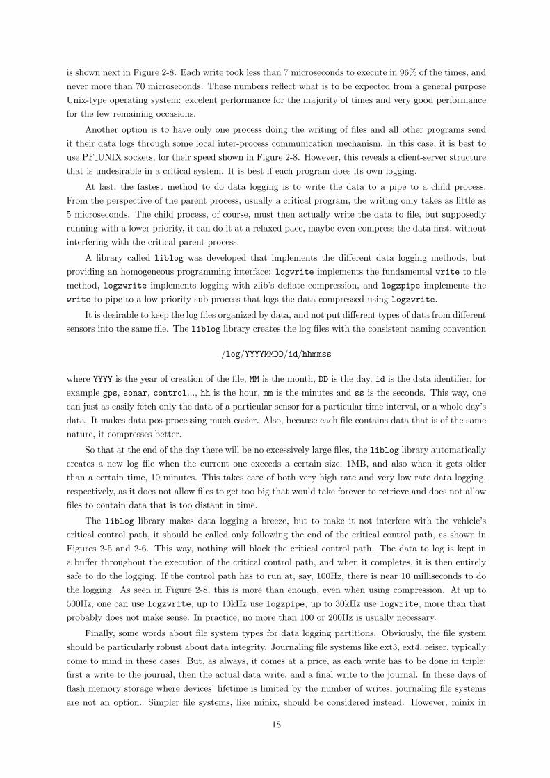
is shown next in Figure 2-8. Each write took less than 7 microseconds to execute in 96% of the times, and
never more than 70 microseconds. These numbers reflect what is to be expected from a general purpose
Unix-type operating system: excelent performance for the majority of times and very good performance
for the few remaining occasions.
Another option is to have only one process doing the writing of files and all other programs send
it their data logs through some local inter-process communication mechanism. In this case, it is best to
use PF UNIX sockets, for their speed shown in Figure 2-8. However, this reveals a client-server structure
that is undesirable in a critical system. It is best if each program does its own logging.
At last, the fastest method to do data logging is to write the data to a pipe to a child process.
From the perspective of the parent process, usually a critical program, the writing only takes as little as
5 microseconds. The child process, of course, must then actually write the data to file, but supposedly
running with a lower priority, it can do it at a relaxed pace, maybe even compress the data first, without
interfering with the critical parent process.
A library called liblog was developed that implements the different data logging methods, but
providing an homogeneous programming interface: logwrite implements the fundamental write to file
method, logzwrite implements logging with zlib’s deflate compression, and logzpipe implements the
write to pipe to a low-priority sub-process that logs the data compressed using logzwrite.
It is desirable to keep the log files organized by data, and not put different types of data from different
sensors into the same file. The liblog library creates the log files with the consistent naming convention
/log/YYYYMMDD/id/hhmmss
where YYYY is the year of creation of the file, MM is the month, DD is the day, id is the data identifier, for
example gps, sonar, control..., hh is the hour, mm is the minutes and ss is the seconds. This way, one
can just as easily fetch only the data of a particular sensor for a particular time interval, or a whole day’s
data. It makes data pos-processing much easier. Also, because each file contains data that is of the same
nature, it compresses better.
So that at the end of the day there will be no excessively large files, the liblog library automatically
creates a new log file when the current one exceeds a certain size, 1MB, and also when it gets older
than a certain time, 10 minutes. This takes care of both very high rate and very low rate data logging,
respectively, as it does not allow files to get too big that would take forever to retrieve and does not allow
files to contain data that is too distant in time.
The liblog library makes data logging a breeze, but to make it not interfere with the vehicle’s
critical control path, it should be called only following the end of the critical control path, as shown in
Figures 2-5 and 2-6. This way, nothing will block the critical control path. The data to log is kept in
a buffer throughout the execution of the critical control path, and when it completes, it is then entirely
safe to do the logging. If the control path has to run at, say, 100Hz, there is near 10 milliseconds to do
the logging. As seen in Figure 2-8, this is more than enough, even when using compression. At up to
500Hz, one can use logzwrite, up to 10kHz use logzpipe, up to 30kHz use logwrite, more than that
probably does not make sense. In practice, no more than 100 or 200Hz is usually necessary.
Finally, some words about file system types for data logging partitions. Obviously, the file system
should be particularly robust about data integrity. Journaling file systems like ext3, ext4, reiser, typically
come to mind in these cases. But, as always, it comes at a price, as each write has to be done in triple:
first a write to the journal, then the actual data write, and a final write to the journal. In these days of
flash memory storage where devices’ lifetime is limited by the number of writes, journaling file systems
are not an option. Simpler file systems, like minix, should be considered instead. However, minix in
18

particular has limitations on file attributes, path name lengths, and automated file system checks and
repairs. Therefore, a good middle-term option is the trustworthy ext2, a full-fledged file system with
good automated checks and repairs, but that does not use a journal.
2.11 Communications
Technically, communications are not allowed on an autonomous vehicle. An autonomous vehicle
should be... autonomous. But in practice, communications are commonly used on autonomous vehicles,
for a number of reasons: to monitor the vehicles’ status, telemetry, to visualize the sensors’ data in
real-time, to modify the missions on the fly, to remotely stop the vehicle in case of emergency, to upload
new versions of programs, to retrieve data log files.
The physical link is generally restricted to wireless, from the ubiquitous IEEE 802.11, to specialized
long-range radios, to dedicated satellite links, up to underwater acoustic modems, in decreasing order of
data rate, from low to lowest. But they are all slow. In fact, wireless communications are usually the
slowest component in the whole software architecture of an autonomous vehicle, so it must be handled
with special care not to block anything in the critical control path.
Just like with data logging, communications should be performed only after the execution of the
critical control path, as shown in Figures 2-5 and 2-6, so that they do not interfere. Whether the
communications are done before or after the data logging depends on the vehicle and its application, and
what is considered more important for the specific mission.
However, while this takes care of communications for the critical program, this measure alone does
not take into account the other programs that may share the same communication channel. It is very easy
to saturate such low-bandwidth wireless connections. When it happens, bulky high data rate programs
will consume most of the bandwith, causing huge delays for bursty low data rate programs. To avoid
this, it is necessary to perform traffic control on the output interface to prioritize the transmission of
critical data over non-critical rata.
Linux has advanced traffic control capabilities, like shaping, scheduling, classifying, policing, marking,
dropping. It is however rather complex to set up properly. Fortunately, there is a much simpler solution
that usually suffices. Most applications use the Internet Protocol (IP). The IP header has a field called
Type Of Service (TOS) that hosts and routers use to differentiate the frames and assign them the
appropriate output priorities. Applications that transmit time-critical data need only set the IP TOS
flag to low delay, IPTOS LOWDELAY, using the setsockopt system call, and the kernel will make sure those
packets will be transmitted first, no matter what.
Figure 2-9 shows a typical situation in autonomous vehicles. A monitoring program transmits a small
packet to the autonomous vehicle, to which it replies with another small packet. This repeats forever at a
low rate. Figure 2-9 shows the round-trip time (RTT) of such two packets, about 100 bytes each, repeated
at 1Hz, through a 100kbit/s radio link. When the link is idle, the RTT is about 40 milliseconds. At time
t = 15s, another programs starts downloading a 1MB data log file from the autonomous vehicle, through
the same link. The link immediately becomes saturated on the downlink direction. Without special care,
the RTT of the small packets reach the 300 milliseconds, which may be unacceptable for critical data.
When the IPTOS LOWDELAY flag is used, the RTT of the small packets never exceed 100 milliseconds. The
IPTOS LOWDELAY flag is a simple and effective method, still widely misknown, to implement time critical
communications with minimum latency guarantees for autonomous vehicles.
19

OffOnIdle
IPTOS LOWDELAY
Time (sec)
RT
T(m
sec)
1501251007550250
350
300
250
200
150
100
50
0
Figure 2-9 IPTOS LOWDELAY performance on low-bandwidth links.
2.12 Profiling
Profiling is a technique for measuring the performance of a program as it executes in the real envi-
ronment. In the age of multi-core, superscalar, deeply pipelined processors and multi-tasking operating
systems, static code analysis of programs becomes meaningless, and is rightly so used for source code
verification only. Therefore, profiling is really the only true way to assert that an autonomous vehicle
meets its specifications.
Yet, most people usually don’t profile their programs, mainly because they have built such complex
software architectures, using concurrent threads, synchronizations, intricate inter-process communica-
tions, that it becomes extremelly difficult to gather any information that could ever be successfully
analysed.
The proposed software architecture, on the other hand, makes it very easy to carry through the
essential profiling of the critical programs of autonomous vehicles. Starting from Figure 2-5, the first step
is to collect timestamps of the program execution at the points of interest. Typically, a timestamp is
collected at the entry point of a function and another timestamp at the exit point, in order to profile that
function’s behaviour. But it is just as easy to profile the whole program altogether, by simply collecting
timestamps at all the transitions.
The timestamps are most easily collected using the gettimeofday system call. It should be noted
that, even though gettimeofday has a resolution of microseconds, some operating systems only provide
millisecond resolution. Linux, compiled with the CONFIG HIGH RES TIMERS option, provides nanosecond
resolution.
At the end of each critical path run, the profiling data is logged together with all the other data.
This way, the impact of profiling on the critical program’s execution is negligible: less than 1 microsecond
per gettimeofday system call.
20

2.13 Simulation
Testing autonomous vehicles in the real world is usually very expensive, in all terms of money, time
and effort. Furthermore, a test gone bad with an autonomous vehicle can cause serious damages, people
including. Therefore, developing a software simulator for an autonomous vehicle is not an indulgence, it
is a true necessity.
The objective of a software simulator for an autonomous vehicle is to be able to run as much as
possible of the exact same code that is going to run on the real vehicle, but without requiring physical
access to the vehicle hardware. This allows conclusive testing of new algorithms for the vehicle with the
touch of a button, as many times as needed, in a safe, practical, accessible, comfortable environment, like
on any desktop or laptop computer. Figure 2-10 depicts software simulation of autonomous vehicles.
Software Simulator
Vehicle
Software
ConsoleSoftware Model Software
External
Communications Actuators
Sensors
Sensors Actuators
SoftwareVehicle
Software Simulator
ConsoleSoftware
Communications
Software
Hardware
Console Computer
Software
Hardware
Sensors Actuators
Vehicle Computer
Communications
Figure 2-10 Software simulation of autonomous vehicles.
On top is the real software and hardware of the autonomous vehicle. The goal is to replace the
hardware components with software and to be able to run both the vehicle computer’s software and the
console computer’s software in a single standard computer with no special hardware requirements. This
is shown in the middle of the figure and involves simulating the hardware sensors and actuators’ data
as well as the physical behaviour of the vehicle, which is admittedly not an easy task, but totally worth
doing. On the bottom is shown a different approach, where the simulation of the interaction with the
sensors and actuators is still performed on the same program as the real code is run, but the physical
behaviour of the vehicle is simulated in a separate program, which communicates with the main simulator
using some inter-process communication mechanism, typically an IP socket.
Figure 2-11 shows the SDL graphical representation for the implementation of a software simulator
of an autonomous vehicle with a built-in model of the physical behaviour of the vehicle.
21

ConsoleHandle
Console
Console
0
Init
Start
0
Control
Timer
StateUpdate
Figure 2-11 SDL of simulator with built-in vehicle model.
The sensors’ input elements and actuators’ output elements from Figure 2-10 are replaced by a timer
input element set to fire at the same frequency as the critical control path of the real vehicle. When
consumed, the timer input updates the state of the vehicle model, simulating an advance in the simulated
world, based on the currently applied actuation. The control procedure, as well as the console handling
procedure, is left exactly the same as those implemented for the real vehicle, so they are effectively being
tested at all times.
The software simulator for an autonomous vehicle using an external vehicle model is shown in
Figure 2-12. In this case, the state of the vehicle is kept and updated in the external model program,
which is sent at the same frequency as the real vehicle’s control path execution to the simulator, consuming
the State input. The exact same control procedure as the real vehicle is then executed, and the calculated
actuation is sent back to the external model program. The console handling is still exactly the same as
in the real vehicle. This simulator with external model can be usefull when using specialized modelling
software, like Octave.
A software simulator of an autonomous vehicle, whether with a built-in vehicle model, or using an
external program to model the vehicle, is of maximum importance, and should be one of the very first
things to implement during the development of the software for an autonomous vehicle.
22

ConsoleHandle
Console
Console
0
Init
Start
0
Control
State
Actuation
Figure 2-12 SDL of simulator using an external vehicle model.
23

24

3DELFIMx
DelfimX is an autonomous catamaran developed at the Dynamical Systems and Ocean Robotics
(DSOR) laboratory of the Institute for Systems and Robotics (ISR) in Instituto Superior Tecnico (IST),
Lisbon, Portugal. It was first put to sea in 2007, featuring a complex software and hardware architecture
inherited from its predecessor Delfim, a smaller autonomous catamaram developed by the same laboratory
in the 90’s. It initially suffered from recurrent problems in part caused by its complex architecture, so it
was later decided that it was best to re-develop the software from scratch using a better approach.
This chapter describes how the software architecture for autonomous vehicles presented in the pre-
vious chapter was successfully implemented for DelfimX. The end result is that DelfimX is currently
operating smoothly, with the added benefit that it was possible to eliminate much hardware that has
now been made unnecessary by the new software. Given the accomplishment, the software of the original
Delfim autonomous catamaran was then also re-implemented using this same software architecture.
Figure 3-1 Delfim (left) and DelfimX (right) autonomous catamarans.
25

3.1 Requirements
The software of the DelfimX autonomous catamaran meets the requirements depicted in Figure 3-2.
Communications
Data logging
SOFTWARE
Radio
Ethernet RS232 Ethernet
WiFiPeripheralsOnboard
IDE
MemoryCard
Sensors
GPS
Navigation
StarboardPropeller
PortPropeller
StarboardBatteries
PortBatteries
ComputerBatteries
CAN CAN
Actuators
StarboardPropeller
PortPropeller
Figure 3-2 DelfimX software requirements.
Shown are the critical sensors only, and for DelfimX these were all designed to have Controller Area
Network (CAN) interfaces, but any number of additional sensors with the most different interfaces should
be supported as well. A usual interface for marine sensors is RS232/422/485.
The main actuators were also designed to have CAN interfaces, but other interfaces should be
supported as well for auxiliar actuators. Usual interfaces for electrical motors and servomechanisms are
RS232 or direct PWM drive.
The primary communication link for DelfimX is a long range radio that has an RS232 interface. At
the software level, it was decided to use the Serial Line Internet Protocol (SLIP) encapsulation for data
multiplexing. Other communication links should also be supported for payload usage, typically WiFi for
close range, higher throughput, remote applications and ethernet for onboard guest applications.
Data logging is to be performed on a flash memory device. Shown is a card with an IDE interface,
but other popular media and interfaces should be supported as well, like the unbelievably small micro-SD
cards and the ubiquitous USB mass storage flash memory devices.
The computer system is a PC/104, for it is easily expandable with stackable peripheral boards to
accomodate such vast diversity of interfaces. The specifications of the DelfimX PC/104 motherboard are:
- AMD Geode LX800 500MHz CPU
- 512MB DDR RAM
- CompactFlash
- Ethernet
- RS232/422/485
The specifications of the expansion PC/104 boards are:
- TS-CAN1 CAN interface board with Philips SJA1000 CAN controller
26

Figure 3-3 DelfimX PC/104 computer.
Plus DC-DC converter board, the total stack size is about 1dm3, which can still be considered
small, by today’s standards, and its average power consumption is 7W during normal operation, which is
passable, considering the 500MHz CPU and 512MB RAM overkill. 50MHz and 8MB, repectively, would
be enough for DelfimX, as shown ahead.
The operational requirements for the DelfimX software is that it must handle navigation data at a
5Hz rate, and for each sample, execute the control algorithm and send the calculated actuation to the
propellers; this defines the critical execution path, and must complete within the 200ms sample interval
time. Data logging is performed after each critical execution path, at the same 5Hz rate, but it is not
considered time-critical, it is only data-critical. At 1Hz, commands are received from a ground console,
which expects the DelfimX software to send back the vehicle state within the next second. All other
sensors send their status at a rate of 1Hz or lower, and the DelfimX software need only check that all
sensors are good, and if not, warn the ground console and stop the vehicle.
Given the computer hardware platform and the operational requirements, the development of the
DelfimX software can start, following the architecture presented in Chapter 2, and noticing how Figure 3-2
matches Figure 2-1 exactly.
3.2 Kernel
The DelfimX operating system kernel is Linux, version 2.6.30, the latest from the stable branch at
the time of writing. Linux supports all the interfaces specified in the requirements, including CAN, out
of the box. Except that most CAN devices used in DelfimX were developed at the DSOR lab and use
special CAN protocols. For these, the CAN implementation developed in Chapter 5 was added to the
Linux kernel to form the final DelfimX Linux kernel. Apart from this CAN patch, the DelfimX kernel is
a plain Linux kernel. The following is a discussion of the most relevant configuration options used when
compiling the DelfimX Linux kernel, as in Section 2.4, but for the particular case of DelfimX.
27

CONFIG PREEMPT NONE, CONFIG HZ 100, CONFIG NO HZ: these options configure the scheduler for max-
imum throughput performance and minimum power consuption, but also for worst rescheduling latency.
This latency was measured for DelfimX during real operation to be 60 microseconds on average and
less than 3 milliseconds on worst case, as detailed in Section 3.5. These values are well within the
DelfimX specified requirements. No real-time kernels are necessary, just a plain Linux kernel with the
most conservative settings.
CONFIG HIGH RES TIMERS: this option enables high resolution timer support, so that one can times-
tamp events with nanosecond resolution. Without this option, the kernel time resolution would be the
same as the scheduler, only 10 milliseconds.
CONFIG INITRAMFS SOURCE, CONFIG BLK DEV INITRD, CONFIG RD GZIP: these options add support for
mounting the root file system, described in the next section, from an initial RAM file system file, loaded
by the boot loader, in cpio format and compressed with gzip. The CONFIG INITRAMFS SOURCE option
alone would allow for embedding the root file system into the kernel image file, which would be more
efficient, however, for an autonomous vehicle, having the kernel and the root file system in two separate
files makes it easier to maintain, as it is rarely needed to update the kernel, while the file system is often
updated, and this way it is not necessary to recompile the whole kernel image every time it is necessary
to update some user program.
CONFIG SLIP, CONFIG SLIP COMPRESSED: these options enable the Serial Line Internet Protocol for
the DelfimX radio communications, using the Van Jacobsen TCP/IP header compression, for faster
transfers. With normal SLIP, the average FTP download data rate with the DelfimX radio is about
6kB/s, whereas with VJ compression it is more than 7kB/s, about 20% speed increase. The effect on
interactive programs, like RSH remote program execution, or CAN monitoring programs, however, is
much more striking, with speed increases of 200% being common.
These are the most critical, or out of the ordinary, configuration options. There are over 300 more
configuration options for the DelfimX Linux kernel. It is not possible to go through them all in here.
They deal mainly with choosing the appropriate drivers for the specific computer hardware platform,
and are standard procedure: CPU model, IDE controller, ethernet controller, serial ports, USB host and
devices, network stack, file systems, etc...
What remains left to discuss are the configuration options not part of the plain Linux kernel, but
that were added by the CAN implementation, detailed in Chapter 5, and that are used in DelfimX.
CONFIG CAN: this option allows the selection of all the Controller Area Network related options.
CONFIG PF CAN: this option adds the CAN protocol family PF CAN demultiplexer to the kernel’s
socket() system call handler.
CONFIG CANPROTO CAN: this option adds the implementation of the CAN 2.0B specification.
CONFIG DSOR: this option allows the selection of the DSOR lab special CAN modules.
CONFIG CANPROTO DSOR: this option adds the implementation of the DSOR higher-layer segmented
messages CAN protocols.
CONFIG DSOR NODE ID=0x00: this option sets the node identifier of the DSOR higher-layer segmented
messages UDP over CAN protocol that DelfimX should impersonate as. 0x00 was the now defunct
gateway microcontroller.
CONFIG DSOR RTIME: this option adds a redundant time service to the DelfimX CAN. The GPS node
transmits a time CAN frame at 1Hz, without which most other nodes will block. This redundant time
service takes over the transmission of the time CAN frame when the GPS node fails to.
CONFIG DSOR VEHICLE=0xc0: this option sets the 8-bit DSOR vehicle identifier (bits 4-7) used for
the identifier of the time CAN frame. 0xc0 is the identifier of the DelfimX.
28
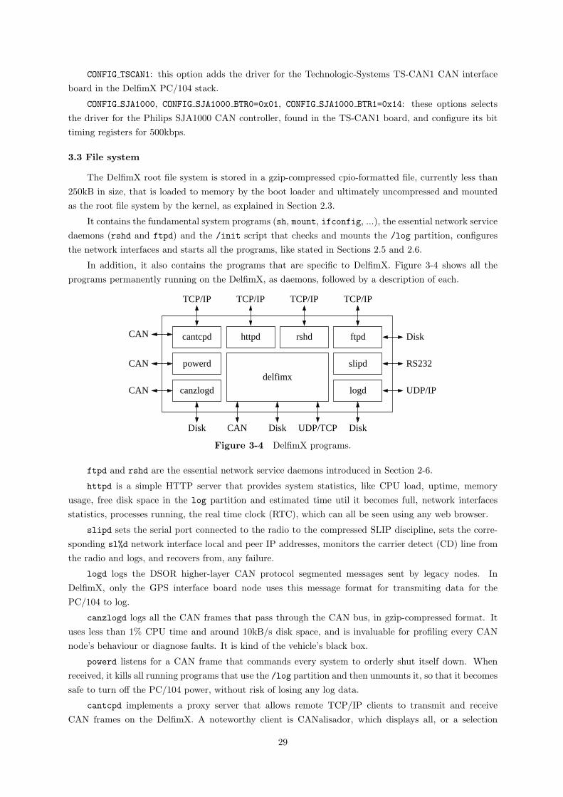
CONFIG TSCAN1: this option adds the driver for the Technologic-Systems TS-CAN1 CAN interface
board in the DelfimX PC/104 stack.
CONFIG SJA1000, CONFIG SJA1000 BTR0=0x01, CONFIG SJA1000 BTR1=0x14: these options selects
the driver for the Philips SJA1000 CAN controller, found in the TS-CAN1 board, and configure its bit
timing registers for 500kbps.
3.3 File system
The DelfimX root file system is stored in a gzip-compressed cpio-formatted file, currently less than
250kB in size, that is loaded to memory by the boot loader and ultimately uncompressed and mounted
as the root file system by the kernel, as explained in Section 2.3.
It contains the fundamental system programs (sh, mount, ifconfig, ...), the essential network service
daemons (rshd and ftpd) and the /init script that checks and mounts the /log partition, configures
the network interfaces and starts all the programs, like stated in Sections 2.5 and 2.6.
In addition, it also contains the programs that are specific to DelfimX. Figure 3-4 shows all the
programs permanently running on the DelfimX, as daemons, followed by a description of each.
canzlogd
cantcpd httpd rshd ftpd
powerd slipd
logd
delfimx
TCP/IP TCP/IP TCP/IP TCP/IP
CAN
CAN
CAN
RS232
UDP/IP
Disk
Disk DiskCAN Disk UDP/TCP
Figure 3-4 DelfimX programs.
ftpd and rshd are the essential network service daemons introduced in Section 2-6.
httpd is a simple HTTP server that provides system statistics, like CPU load, uptime, memory
usage, free disk space in the log partition and estimated time util it becomes full, network interfaces
statistics, processes running, the real time clock (RTC), which can all be seen using any web browser.
slipd sets the serial port connected to the radio to the compressed SLIP discipline, sets the corre-
sponding sl%d network interface local and peer IP addresses, monitors the carrier detect (CD) line from
the radio and logs, and recovers from, any failure.
logd logs the DSOR higher-layer CAN protocol segmented messages sent by legacy nodes. In
DelfimX, only the GPS interface board node uses this message format for transmiting data for the
PC/104 to log.
canzlogd logs all the CAN frames that pass through the CAN bus, in gzip-compressed format. It
uses less than 1% CPU time and around 10kB/s disk space, and is invaluable for profiling every CAN
node’s behaviour or diagnose faults. It is kind of the vehicle’s black box.
powerd listens for a CAN frame that commands every system to orderly shut itself down. When
received, it kills all running programs that use the /log partition and then unmounts it, so that it becomes
safe to turn off the PC/104 power, without risk of losing any log data.
cantcpd implements a proxy server that allows remote TCP/IP clients to transmit and receive
CAN frames on the DelfimX. A noteworthy client is CANalisador, which displays all, or a selection
29

of, the DelfimX CAN traffic in real-time, remotely, during vehicle operation. Another useful client is
avrcanisp, which allows remote in-system-programming of the DelfimX AVR CAN microcontrollers.
Finally, delfimx is the vital program, the brains, of DelfimX. It is responsible for much of the
vehicle’s operational requirements and its implementation is dissected in the next section. The delfimx
process is run with niceness 0 (normal priority), while all other processes are run with nicer values (lower
priorities).
Except for the sh Bourne shell and the e2fsck ext2 file system checker, all programs in DelfimX
were written from scratch by the author of this thesis.
3.4 Implementation
The implementation of the DelfimX’s critical program delfimx follows the rationale presented in
Section 2.7 that it should be a single process. Then, starting from the operational requirements and
from Figure 3-1, the next step of the software development is to assign each requirement, device, or
functionality to a separate block, or module, or, in this case, a separate C source file that implements
just that requirement, device or functionality, and that alone. Figure 3-5 shows all the C source files that
make up the delfimx program.
sysstat.c
navcan.c
Sensors
main.c
control/*.c
prop.c
Actuators
grex.c
Communications
console.c
log.c
Data logging
Figure 3-5 DelfimX source code files.
navcan.c implements the reading of the navigation data from a CAN socket and updating the
DelfimX state with the data read.
sysstat.c implements the reading of all the other sensors’ data, as they all come from the same
DSOR-specified CAN frame called sysstat (system status), from a CAN socket. Actually, they are two
CAN sockets, one to receive segmented sysstat CAN messages, from the GPS, and one to receive the
extended sysstat CAN frames, from all the other sensors, but both CAN sockets are read using the
exact same function and further equally handled.
prop.c implements sending the propulsion actuation commands to the starboard and port propellers,
through a CAN socket. The CAN frames’ data is the same for both propellers, only the CAN identifiers
change, thus both are implemented on the same source file.
log.c implements the writing (appending) of the current DelfimX state to a log file, using the liblog
library from Section 2.10, creating new log files when the current one grows too large or too old.
30

console.c implements the reading of the commands sent by the console and the transmission of the
current DelfimX state back to the console, through an UDP/IP socket, be it from the radio or ethernet.
grex.c implements the communication with an onboard guest computer called GREX, an european
project where DelfimX is currently involved. The delfimx program acts as a TCP/IP server that the
GREX computer connects to. From then on, delfimx proxies the navigation data to the GREX computer
and, when DelfimX is in GREX mode, the GREX computer sends heading reference commands for
delfimx to follow.
The control/ directory contains the C source files for all the different control modes of DelfimX,
one file for each. The control/control.c file is the DelfimX control multiplexer that executes the
appropriate control function in one of the other control/*.c files, depending on the current DelfimX
control mode. The currently implemented controllers are: heading (control/heading.c), go to way-
point1 (control/goto1.c), play mission (control/play.c), GREX (control/grex.c) and path follow-
ing (control/pathfol.c). The path following controller was implemented by Rita Cunha, Ph.D.
Finally, main.c implements the delfimx main() function, which glues together all the code in all
the other C files. This is a critical part of the code, and has the potential to become very complex if not
properly implemented. However, when the architecture of Section 2.7 is followed, it turns out to be very
simple to implement efficiently, as shown in Figure 3-6.
Navigation
SysStat
Console
GREX
delfimx
Process
Log
Console
GREX
Propulsion
Figure 3-6 DelfimX single process, inputs and outputs.
The delfimx main() is implemented simply as a function of its inputs and outputs. Its SDL graphical
representation is shown in Figure 3-7. It should meet all the operational requirements set for DelfimX in
Section 3.1. Checking them one by one:
The critical part is the reception of navigation data, processing it, executing the control algorithm,
and sending the actuation commands to the propulsion. This is clearly described in the SDL graphic
representation in Figure 3-7 by the consumption of the navigation signal, execution of the navigation
procedure, execution of the control procedure, and sending of the propulsion signal (leftmost branch of
the figure). Following is the non-critical sending of the GREX signal, not included in the original DelfimX
requirements but added a posteriori, and the log signal, which corresponds to the requirement of data
logging the DelfimX state at the navigation’s rate.
The consumption of the SysStat signal and execution of the SysStat procedure (the next branch in
the figure) describes the requirement of receiving every sensors’ data and checking it.
The DelfimX requires that a console sends it commands, which it acts upon, and then sends back its
status to the console. This is described by the consumption of a console signal, execution of the console
command procedure, sending of the propulsion signal, and finally sending a console status signal back
to the console (the branch in the middle of the figure). It may not be obvious why the sending of a
propulsion signal is in here. The reason is that one of the possible commands sent by the console is a
direct manual command for the propellers, in which case it should be executed here, independently of
the navigation branch.
31

0
Init
Start
SysStatHandle
SysStat
Navigation
Navigation
Control
Log
Handle
GREX
Console
Console
Propulsion
GREXHandle
GREX Watchdog
Stop
Propulsion
Propulsion
HandleConsole
0
Figure 3-7 SDL of DelfimX main function.
The consumption of the GREX signal and execution of the GREX procedure (the next branch in the
figure) was added a posteriori. It describes the reception of commands from the onboard guest GREX
computer, and acting upon them when the DelfimX is in GREX mode.
Finally, as a safety measure, the consumption of a watchdog timer signal executes a procedure that
stops the DelfimX and sends the stop propulsion signal (the rightmost branch in the figure). This happens
if either the navigation or the console fail to send any data to the delfimx program for more than some
specified time, in which case it stops DelfimX and does not let it go adrift.
It should be noted that this SDL process has one single state. There are no intermediate states that
could otherwise block the process execution and make it miss a deadline. Furthermore, in SDL, the signals
are consumed, processed, sent, and here it transitions back to the initial state, atomically. But computers
take a non-zero time to execute this code, though it is in the order of microseconds, occasionally a few
milliseconds, maximum, as shown in the next section, which is orders of magnitude below the DelfimX
critial path’s 200ms deadline limit. This assures that the delfimx program will always meet the DelfimX
timing requirements, unless of course something is implemented wrong.
Moving on to the real code, implementing code starting from an SDL graphic representation is
straightforward, as seen in Section 2.7 Figure 2-6. The following is the real implementation of the
32

delfimx program main() function, as specified in the SDL of Figure 3-7, and it is the implementation
currently running on DelfimX.
int main()
{
struct delfimx delfimx;
struct pollfd pfd[N];
init(&delfimx, &pfd);
for (;;) {
poll(pfd, N, TIMEOUT);
if (pfd[0].revents) {
navigation(pfd[0].fd, &delfimx);
control(&delfimx);
propulsion(&delfimx);
grex send(&delfimx);
log(&delfimx);
}
if (pfd[1].revents)
sysstat(pfd[1].fd, &delfimx);
if (pfd[2].revents)
sysstat(pfd[2].fd, &delfimx);
if (pfd[3].revents) {
console read(pfd[3].fd, &delfimx);
propulsion(&delfimx);
console write(pfd[3].fd, &delfimx);
}
if (grex poll(pfd+4, pfd+5))
grex recv(&delfimx);
if (watchdog()) {
stop(&delfimx);
propulsion(&delfimx);
}
}
}
Figure 3-8 C implementation of the main of DelfimX.
That’s it! It feels rather disappointing, but it really can be this simple to implement the critical
software architecture for an autonomous vehicle. Of course, it takes hard work to arrive at such simplicity.
Most inexperienced programmers would develop overly complex implementations that would hardly ever
function properly. But if the software architecture for autonomous vehicles presented in the previous
chapter is followed, it is difficult to go astray.
33

3.5 Profiling
The moment of truth! Although it is pretty certain that the delfimx program just developed
meets all the time critical requirements, because it was carefully implemented following the architecture
presented in Chapter 2, it is always mandatory to profile a program’s execution in the real world, as it
is the only honest way of proving it. As discussed in Section 2.12, a simple way to profile the critical
execution path of the delfimx program is to insert a few gettimeofday system calls to timestamp the
beginning and end of the events of interest. For delfimx, this simply becomes:
int main()
{
...
for (;;) {
poll(pfd, N, TIMEOUT);
if (pfd[0].revents) {
gettimeofday(&delfimx.profile.t1);
navigation(pfd[0].fd, &delfimx);
gettimeofday(&delfimx.profile.t2);
control(&delfimx);
gettimeofday(&delfimx.profile.t3);
propulsion(&delfimx);
gettimeofday(&delfimx.profile.t4);
log(&delfimx);
gettimeofday(&delfimx.profile.t5);
}
...
}
}
Figure 3-9 Profiling the delfimx critical execution path.
It becomes that the navigation function takes (t2 − t1)µs to execute, control takes (t3 − t2),
propulsion takes (t4 − t3), and log takes (t5 − t4), for each run of the critical path code.
What is missing now is t0. The execution of the critical path is triggered by the reception of a
sequence of CAN frames sent by the navigation microcontroller node. Therefore, the best estimate for t0
is the time instant that the PC/104’s CAN controller generates the hardware interrupt that signals the
reception of the last CAN frame in the sequence. The CAN controller drivers implemented in Chapter 5
stamp all CAN frames’ reception times in the interrupt service routine, so that user programs can use
them to accurately reference every CAN frame in time. In DelfimX, the canzlogd program, presented in
Section 3.3, logs all CAN frames’ data, along with their reception timestamps. t0 is thus obtained from
the canzlogd log files, as the timestamp of the last CAN frame received in the sequence of navigation
CAN frames. So, finally, the entire operating system latency, from the time the CAN frame reception
hardware interrupt is handled until the time the navigation function in the delfimx process actually
starts executing, is exactly (t1 − t0)µs. This interval is referred to as poll in the following plots, for
simplicity, but it is not merely the time the poll function takes to execute, it has all the meaning just
mentioned.
Furthermore, the total latency of the DelfimX critical execution path, defined as the time the naviga-
tion microcontroller sends its last CAN frame until the time the delfimx program computes and transmits
34

the propulsion actuation command CAN frames, is (t4− t0)µs. This value is plotted in Figure 3-10, as an
histogram, for 150645 consecutive runs of the delfimx critical path during real operation at sea. Since
the navigation sends data at 5Hz, that ammounts to a very significative 150645/5/3600 ≈ 8.4 hours of
continuous operation on a real environment.
Critical path (poll+navread+control+prop) latency
Latency (msec)
Sam
ple
s
10.1 2.70.50.20.05
105
104
103
102
101
100
Figure 3-10 DelfimX critical path execution times.
In more than 99.3% of the times, the full critical path takes 100µs or less to execute (it should be
noted that the axis scales are logarithmic). This totally confirms the initial conviction that the DelfimX
requirements are no challenge whatsoever for this software architecture, proposed in Chapter 2. One
could easily handle a vehicle with requirements one thousand times more demanding, literally.
There are a few outliers, of course, as expected from any general purpose operating system. However,
only in less than 0.7% of the times it took more than 1µs, yet less than 1ms, to finish. And only in
1 out of 150645 runs (that is less than 10ppm, parts-per-million) it exceeded 1ms. It took 2.674ms,
to be precise. That is still miles away from the 200ms limit set in the DelfimX requirements. Even if
the specified limit had been 1ms, which would be overkill even for the most demanding vehicles, like
helicopters, this program still provided a better than 10ppm accuracy. It is therefore highly unreasonable
to invoke the need for any real-time kernel.
For comparison, Figure 3-11 shows the execution times of the various stages of the delfimx program’s
critical execution path, plus the log function for completeness, averaged over all those 8+ hours of
execution.
The stage that takes the longest is poll: reading the last CAN frame from the CAN controllers
registers in the interrupt service routine, assembling the full CAN segmented message in a software
interrupt, delivering it to the appropriate socket buffer in kernel space, and switching context to the
delfimx user process waiting for input on the socket. Even all this, it is only about 57µs.
The navigation stage basically takes the time of the read system call that reads the complete CAN
segmented message from the CANsocket: about 6µs.
The control stage does not invoke any system call and is thus the fastest. Its execution time depends
only on the complexity of the algorithm and how well it is implemented. In delfimx, all control algorithms
35

are very simple, and take a mere 2µs to execute, even though they call transcendental trigonometric
floating-point instructions that take hundreds of clock cycles to execute on dedicated hardware.
Critical path stages average execution time
use
c
logpropcontrolnavreadpoll
60
50
40
30
20
10
0
Figure 3-11 DelfimX critical blocks average execution times.
The propulsion stage consists of four write system calls to the kernel CAN socket layer, to send
the four actuation command CAN frames (one to the starboard propeller microcontroller, one to the
starboard propeller batteries microcontroller, one to the port propeller microcontroller, and one to the
port propeller batteries microcontroller). It all takes about 24µs.
The critical path ends here, but it is still needed to log this iteration’s data, although at a relaxed
pace, if one wishes so. The log stage involves, for most of the times, a single write system call to write the
log data to the appropriate kernel block driver that will eventually write the data to the CompactFlash
card. Occasionally, it also involves calling the close and open system calls to close the current log file,
when it exceeds a certain size or age, and create a new one. On average, the log stage takes 19µs.
In sum, the profiling of the delfimx program in real world operation demonstrates that it fulfills all
DelfimX operational timing requirements with great ease.
3.6 Simulator
DelfimX is a big boat. It requires heavy logistics, many people, hundreds of Euros to put it in the
water for only a few hours tests. It is inconceivable having to go through all this just to run a piece of
software. Therefore, a couple of DelfimX simulators have also been developed that have proven to be
extremely useful.
Like discussed in Section 2.13, the objective of the DelfimX simulators is to be able to run as much
as possible of the exact same code that is going to run on DelfimX, but in a safe, practical, accessible,
comfortable environment, like on any desktop or laptop computer, enabling the programmer to quickly
experiment new code and thoroughly test it, which avoids going to the water with untested software,
wasting everyone’s time, and essentially making a foul out of him. Figure 3-12 is an overview for the
software simulation of DelfimX.
36

Software
Hardware
DelfimX Computer
Software
Hardware
Console Computer
Software
Hardware
GREX Computer
Sensors ActuatorsCommunications
DelfimX
Communications
SoftwareDelfimX
Software Simulator
GREXSoftware
ConsoleSoftware
Communications Communications
SoftwareDelfimX
Software Simulator
Sensors Actuators
GREXSoftware
ConsoleSoftware
Communications Communications
ActuatorsSensors
Model SoftwareExternal
Figure 3-12 DelfimX software simulation.
On top is the real software and hardware of DelfimX. The complete operational setup is made up of
three main computers, each with its own specific hardware: hardware for communications between the
console computer and the DelfimX computer, hardware for communications between the GREX computer
and the DelfimX computer, and, most importantly, hardware for interfacing the DelfimX sensors and
actuators. The goal is to replace all this hardware by software.
In the middle of the figure is the DelfimX simulator with a built-in model. The communications
between the three computers are replaced with local software connections, making it possible to run the
complete DelfimX operational setup on a single computer at any desk. The built-in model simulates the
physical behaviour of the vehicle, the sensors’ data and the actuators’ response.
On the bottom is the DelfimX simulator with an external model. In this case, the simulator replaces
the sensors and actuators’ interfaces with a local software connection to a separate program, which then
simulates the physical behaviour of the vehicle, the sensors’ data and the actuators’ response.
37

3.6.1 Simulator with built-in model
The source code structure of the DelfimX simulator with built-in model is shown in Figure 3-13.
model.c
control/*.c
grex.c
Communications
console.c
Figure 3-13 DelfimX simulator with built-in model.
Comparing with Figure 3-5, the source code structure of the real DelfimX software, the sensors,
actuators and log source code was replaced by the model.c file. All the other files are the same as in the
real DelfimX. This means that this simulator runs the exact same console communication code, GREX
communication code and DelfimX control algorithms code as the real DelfimX. Figure 3-14 is the SDL
graphic representation of the implementation of model.c.
0
Init
Start
Console
GREXHandle
GREX
HandleConsole
Console
State
Timer
Control
GREX
Update
0
Figure 3-14 SDL of DelfimX simulator with built-in model.
The sensors’ input elements and actuators’ output elements from the SDL of the real DelfimX
main.c function, in Figure 3-7, are replaced by a timer input element, firing at the same 5Hz frequency
38

as the real navigation system. When consumed, the timer input executes the update state procedure
that simulates a 200ms advance in the internal state of the DelfimX, based on the currently applied
actuation. This simulation includes the DelfimX physical dynamics (linear and angular positions and
velocities), conversion to sensors and actuators’ units (GPS coordinates, propellers’ RPM), and external
forces (wind or water current). The details of the model’s implementation are not delved in this thesis.
That alone is usually the subject of whole PhD thesis. It suffices that the model that was implemented
for the DelfimX simulator is a good working approximation of the behaviour of the real DelfimX at sea,
and all in just a few simple C functions of half a dozen lines each, so it is trivial for anyone to further
extended the model to simulate more parameters, if it really becomes necessary.
3.6.2 Simulator with external model
The DelfimX simulator with built-in model is utmost practical: it is a single program and it is
implemented in C. Still, there was popular demand for a DelfimX simulator that implemented everything
but the vehicle model, and allowed the model to be implemented in a separate program, in whatever
language one prefers. Figure 3-15 shows the source code structure of the DelfimX simulator with external
model.
extmodel.c
control/*.c
Sensors
grex.c
Communications
console.c
Actuators
ExternalModel
External
SoftwareModel
Software
Figure 3-15 DelfimX simulator with external model.
Just like the simulator with built-in model, the sensors, actuators and log code from the real DelfimX
in Figure 3-5 was replaced. This time, by code in the extmodel.c file, which instead receives the vehicle
state data from an external program through an UDP/IP socket and replies with the corresponding
actuation data. The console communications, GREX communications, and all control algorithms are still
exactly the same as the real DelfimX code. Figure 3-16 shows the SDL graphic representation of the
extmodel.c implementation.
Although not as practical as the simulator with built-in model, this DelfimX simulator with external
model can be usefull for integrating the real DelfimX code with specialized modelling software.
39

0
Init
Start
Console
GREXHandle
GREX
HandleConsole
Console
State
Control
Actuation
GREX
0
Figure 3-16 SDL of DelfimX simulator with external model.
40

4Console
The user interface to an autonomous vehicle is historically called the console, and the consensus that
an autonomous vehicle is only as useful as its user interface shows just how important the console is. It
provides to a human operator the power to easily program complex missions, offline, and then remotely
monitor the vehicle during real operation, interact with the onboard sensors and actuators, change mission
parameters, or even the entire mission, on the fly, to adapt to the different facing scenarios.
This chapter discusses the development of a multi-vechile console, and its current use for the Delfim
and DelfimX autonomous catamarans.
4.1 Requirements
As usual, the obligatory first step in the development of a console, or any other product in general, is
to establish its requirements. The keyword is, once again, simplicity. It should be simple, and even fun,
to use the console. Failing this basic requirement, nothing else matters, the console is worthless. Keeping
this in mind, the full list of requirements (sorted by relevance, most important first) for a console for
autonomous vehicles is:
1. the entire console is lightweight, trouble-free to transport, quick to deploy and easy to use;
2. monitor and control multiple vehicles simultaneously;
3. support diverse communication links (ethernet, RS232 radio, WiFi, ...);
4. a display to show, primarily and at all times, the whole mission, and secondarily, the minimum
indispensable vehicles telemetry data (the focus is on the whole mission, not on individual vehicles);
5. optimise display real estate (no title bars, no menu bars, no tool bars, no superfluous vehicle telemetry
data);
6. offline or on-the-fly loading, saving and full editing of missions using any pointing device with a
single button (to be compatible with touchscreens);
7. otherwise fully controllable using keys only (no pointing devices required to operate vehicles);
8. platform-independent (run on Linux, MacOSX and other Unix-like desktop operating systems, em-
bedded and mobile operating systems such as Symbian, or even Windows operating systems);
9. low cost.
41

4.2 Hardware
The console is part hardware, part software. The hardware part should be kept to an absolute
minimum, use off-the-shelf components in every way possible, and simply let the software do the real
work. This immediately makes the console portable and inexpensive, but most importantly, it greatly
reduces the development times, and costs consequently, since changing a line of code takes seconds,
literally, whereas changing hardware could take days, weeks, months. This is basically why they invented
software, half a century ago.
For the console hardware, all that is really needed is a laptop. It has a display, a keyboard, a
pointing device, several communication interfaces (ethernet, WiFi, bluetooth, USB), everything in the
requirements, and it is accessible at any computer store.
Although a laptop is usually all that is necessary for the console of most autonomous vehicles, special
applications may require additional hardware for the console, for instance a long range communication
link, a vehicle-specific human interface controller (joysticks, pedals), an external giant touchscreen. These
can all be easily connected to one of the console laptop’s many interfaces, typically the ubiquitous USB.
Figure 4-1 shows a picture of the console for both Delfim and DelfimX autonomous catamarans.
It is just a small laptop, a 60-mile range radio, connected through USB, and its antenna. The radio
communicates to both catamarans in a point-to-multipoint mode, allowing the console to monitor and
control both catamarans, and more, simultaneously, for cooperative multi-vehicle missions.
Figure 4-1 Console hardware: laptop, radio, antenna.
42

4.3 Software
What really makes the console happen is the software part. Unlike with the software running on
the vehicles, which was meticulously assembled piece by piece in Chapters 2 and 3, from compiling the
kernel, putting together the whole root file system, implementing all the required programs, with full
control over the whole process, for the console software it is not usually required such superlative control.
Therefore, one should rely as much as possible on already existing software. This greatly simplifies the
development of the console software. For example, it allows the developed console software to run on
nearly every portable computer on the market today, meeting the platform-independence requirement set
above, with near zero additional development costs. Figure 5-2 is a screenshot of the console application,
monitoring the Delfim and DelfimX autonomous catamarans.
Figure 4-2 Console screenshot.
The console application resembles very much an ordinary graphical application present in everyone’s
desktop computer. Indeed, its main requirement is to be user-friendly. But all the other requirements
for a console of autonomous vehicles is also met: the central area of the application shows the mission
(the map, the waypoints, the vechiles’ past, present and future locations, obstacles) and on the left side
is the vehicles’ minimum indispensible telemetry data, in particular the propellers’ speed graphs (the
propellers are the components that usually fail the most); there are no title bars, menu bars, or tool bars
that only consume precious screen space; all actions, including loading, saving and full mission editing,
are performed simpply by clicking on the map or desired objects and selecting the appropriate items in
the popup-menus, as shown in Figure 4-3, which is particularly convenient for touchscreens.
43

Figure 4-3 DelfimX pop-up menu screenshot.
The vehicles are fully controllable using the keyboard only, with just a small number and easy to
memorise single-key shortcuts, which are also shown in the popup-menus for reference, as in Figure 4-3.
This makes the console very simple, fast and foolproof to operate even in the most adverse conditions,
like in small boats on open sea. The full list of keys for controlling the Delfim and DelfimX autonomous
catamarans is:
Tab Change keyboard focus to the next vehicle
I Idle mode (thrusters are powered off)
M Manual mode (thrusters are manually set at the console)
H Heading mode (autonomously follow a specified heading)
G Go to waypoint1 mode (go to waypoint1 in heading mode and stop there)
P Path following mode (follow the path connecting the waypoints)
Y Play mission mode (go to each succeding waypoint in heading mode)
X GREX mode (do what the onboard GREX computer says)
R Reset peripheral microcontrollers
0 Set speed to 0%
1 Set speed to 10%
2 Set speed to 20%
...
8 Set speed to 80%
9 (does nothing, for safety, as it is right next to the 0 key)
Up Increase common speed by 1%
Down Decrease common speed by 1%
Right Increase differential speed (turn to starboard side)
Left Decrease differential speed (turn to port side)
Alt Key modifier to select only the starboard thruster, instead of both
Ctrl Key modifier to select only the port thruster, instead of both
44

The console application is built upon Qt and is accordingly implemented in C++. Qt is a cross-
platform application and user interface framework, or simply a library, that makes it easy to write portable
graphical applications which can be deployed across different desktop, mobile and embedded operating
systems without rewriting source code. The task of the application programmer, in this case, is to write
as little code as possible by using as much of Qt’s already written, and tested, code.
The implementation of the console application is object-oriented. Figure 4-4 shows the UML class
diagram of the main, or higher-layer, classes of the console application.
Delfim ViewQDockWidget
QAction Window
QApplication QMainWindow QUdpSocket
Socket
Figure 4-4 Console main window UML class diagram.
The Qt’s QApplication class starts the application creating the console’s single window, an object
of class Window, a subclass of Qt’s QMainWindow. Each keyboard shortcut and popup menu item
action is a QAction object. A single Socket object, a subclass of QUdpSocket that enables the IP-
TOS LOWDELAY flag discussed in Section 2.11, is used to communicate with all vehicles. Each vehicle
has a QDockWidget to display its telemetry data, and it can be docked anywhere on the Window, usually
on the left side, as shown in Figure 4-2. The Window can have any number of vehicle objects. In this
case two Delfim objects, one for the (white) Delfim catamaran, and another for the (yellow) DelfimX
catamaran. The whole mission scene is displayed on the Window by a View object.
The View class makes use of Qt’s Graphics View framework, which implements the viewing, managing
and interaction of a large number of graphical items on a common scene. Figure 4-5 shows the UML
class diagram of the console application’s Graphics View derived classes to view and interact with the
missions, vehicles, and other objects.
Delfim ObstacleWaypoint
DelfimX
View Scene
QGraphicsView QGraphicsScene QGraphicsItem
Figure 4-5 Console graphics scene UML class diagram.
45

The View class is a subclass of Qt’s QGraphicsView class. It displays the full contents of the scene
over a geo-referenced image background, with zooming in, out, and warping to any vehicle with the
touch of a key (Tab). The Scene class, a subclass of Qt’s QGraphicsScene, implements the mission scene
displayed by the View class, and manages all the objects in the scene, which are instances of Qt’s QGraph-
icsItem. The Delfim class, Waypoint class and Obstacle class are thus subclasses of QGraphicsItem.
The QGraphicsItem is the superclass of all graphic items in Qt’s Graphic View framework. Figure 4-6
shows the UML class diagram of the graphic item classes in the console application.
QGraphicsItem
QGraphicsSimpleTextItem
QGraphicsShapeItem
QGraphicsPixmapItem
QGraphicsLine QGraphicsLineItem (Course) Item (Reference)
DelfimTrack Waypoint
QDockWidget Tachometer
QWidget
Figure 4-6 Console graphics items UML class diagram.
The Delfim class is a subclass of QGraphicsPixmapItem. It displays a pixmap image file, an icon
of the vehicle, which is continuously rotated or otherwise transformed to reflect the current, real state
of the vehicle, in this case its yaw. Associated with each vehicle object is: its Track, a subclass of
QAbstractGraphicsShapeItem that displays the vehicle’s past positions as a line; its course, an instance
of QGraphicsLineItem that displays the vehicle’s current course, which is different and usually more
significant than its yaw; its reference, an instance of QGraphicsLineItem that displays where the vehicle’s
autonomous control is going; and any number of Waypoints, subclasses of QGraphicsSimpleTextItem that
display the various waypoints that make up the vehicle’s mission, shown as ordered numbers. Included in
the Delfim’s QDockWidget is a Tachometer that displays a continuous scrolling graph of the vehicle’s port
and starboard thrusters revolutions per minute (rpm). It provides an immediate visual indication of the
vehicle’s well being and sane autonomous control behaviour, and has proven invaluable in the field. Both
QDockWidget and Tachometer are subclasses of QWidget, the base class of Qt’s User Interface framework,
elegantly showing the symbiosis between Qt’s Graphics View and Qt’s User Interface frameworks.
46

4.4 Future work
The possibilities for the console are endless. Above all, the work developed in this chapter introduces
the concept of a software-based console for autonomous vehicles and provides an effective implementa-
tion that can be easily extended to support additional requirements and specific missions and/or vehicles.
Future work might involve, for instance, adding QDockWidgets with live video feeds from onboard cam-
eras on the vehicles, overlaying ladar or sonar live data over the background geo-referenced image map
of the QGraphicsView, implementing a 3D grphics view of the mission scene, for aerial vehicles, using
OpenGL and QGLWidget, playing sound warnings of malfunctions in addition to visual warnings, speech
recognition of the human operator’s commands... Imagination has no limits.
47

48

5Linux CAN
The development of software for autonomous vehicles often include implementing new device drivers,
at the kernel level, for specialised hardware present in the vehicles. An example is the Controller Area
Network (CAN), a communications bus commonly used in autonomous vehicles to interconnect the various
sensors and actuators, but which currently lacks streamlined driver support in modern operating system
kernels.
This chapter presents, first, a new Portable Operating System Interface (POSIX) -compliant Appli-
cation Programming Interface (API), based on the Berkeley socket paradigm, for use in real-time CAN
applications such as autonomous vehicles, and second, a complete implementation of a CAN subsystem
for the Linux kernel, including network device drivers for PCI, ISA and PC/104 cards featuring the Intel
82527 and the Philips SJA1000, the two most popular stand-alone CAN controllers on the market, and
a CAN loopback device driver for all round development tests, the full CAN protocol stack handler for a
whole CAN protocol family of sockets, the data link layer protocol of the CAN specification version 2.0,
both parts A and B, a higher-layer CAN protocol that includes network and transport layers developed
and extensively used at the Dynamical Systems and Ocean Robotics (DSOR) laboratory of the Institute
for Systems and Robotics (ISR), and a few critical CAN services typically needed in autonomous vehicles.
49

5.1 Controller Area Network
Controller Area Network (CAN) is a communication bus especially fit for real-time networked sys-
tems. It was originally developed for use in cars, as a vehicle bus, but it is now also being used for many
other control applications in industrial environments. The specification of CAN defines the data link
layer and the physical layer of the Open Systems Interconnection (OSI) reference model, but allows the
application to choose the electrical properties that are most adequate for the transmission medium.
CAN is a Carrier Sense Multiple Access (CSMA) bus, meaning that there may be several nodes on
the bus, listening, and any one can start transmitting when the bus is idle. Collisions are resolved by
Arbitration on Message Priority (CSMA/AMP): each frame has a static priority, defined by its identifier,
and if two or more nodes start transmitting at the same time, those with lower priority frames immediately
abort, while the highest priority frame continues its transmission. Thus, neither information nor time is
lost. This and a maximum frame data field of 8 bytes provide the necessary guarantees of latency times
required by real-time networked systems.
The identifier of a frame, besides setting the frame’s priority, indicates the meaning of the frame, and
not its source or destination. Receiving nodes use the identifiers to filter which frames are meaningful to
them, and which are not. This feature can be used to create multicast groups, where multiple nodes act
upon simultaneous reception of a frame, for distributed or redundant real-time systems.
CAN implements several safety measures that are important in critical systems. Each node performs
error detection on all frames, error signalling of corrupted frames, re-transmission of faulty frames, and
self-checking of permanent defects that would compromise the bus. All these properties make CAN very
robust and, therefore, widely used in autonomous vehicles.
5.2 CAN Socket API
There is currently no standard Application Programming Interface (API) for CAN. Device manufac-
turers sometimes provide drivers for each device they sell, and different drivers usually present different
APIs, which is almost always the case for different manufacturers. This makes it impossible to develop
CAN applications that are device-independent. There are open projects developing drivers, with a com-
mon API, that support multiple CAN devices. But often, the API is operating system specific, which
means that CAN applications developed with that API would be non-portable. Still other projects im-
plement drivers that use a standard API, typically the open, read, write, ioctl functions. But in this
case, higher-layer CAN protocols are implemented in user-space, usually in the form of libraries, with yet
another unfamiliar API, which also incurs severe performance penalty caused by the constant user-space-
to-kernel-space-and-back memory copies and context switches during frame fragmentation/reassembly in
an eventual implementation of transport-layer messages with more than 8 bytes.
The Berkeley socket paradigm is a mechanism for inter-process communication across computer
networks. Originally developed over two decades ago, it has become the de facto standard, being currently
implemented on just about every computer on the Internet. Its popularity is due to the great simplicity
and versatility of the design.
The socket API is defined in the Portable Operating System Interface (POSIX) specification, which
also makes it portable throughout all POSIX-compliant operating systems, providing source code com-
patibility. POSIX, incorporated in the Single Unix Specification version 3 (SUSv3), is a collection of
standards that defines the API to the operating system, including real-time services and extensions, to
promote software portability across the many POSIX-compliant operating systems.
The socket mechanism is usually implemented at the operating system kernel level, for efficiency.
Embedded devices without operating system can use a smaller footprint implementation instead, and
50

still benefit from the ease-of-use and portability of application development with sockets.
Since sockets are completely protocol-independent, they can be used for any network and protocol,
such as CAN. This section describes how CAN applications could use the socket API, embracing it as
the standard software interface for CAN, being easy-to-use, flexible, efficient and portable. It is written
in the form of a specification proposal, or better yet, a CAN extension to the POSIX specification, that
explains the underlying rationale, making it useful for CAN application developers as a reference manual.
5.2.1 Socket
The CAN application entry-point to the operating system’s socket layer is created with the function:
#include <sys/socket.h>
int socket(int domain, int type, int protocol)
The symbolic constant PF_CAN, to be defined in <sys/socket.h> with an implementation-defined
value, is passed as the domain argument, to specify the creation of a socket in the CAN communications
domain. The type argument is SOCK_RAW, meaning that the application will be interacting directly with
the CAN data link layer. The protocol argument is CANPROTO_CAN, to indicate the protocol in the CAN
specification version 2.0. If successfull, the return value is a non-negative integer: the socket descriptor.
Otherwise, −1 is returned and errno set appropriately.
5.2.2 Socket address
The CAN serial communication link is an implementation-dependent bus channel that carries bits,
where a dominant bit prevails over a recessive bit when transmitted simultaneously. Oblivious to the
actual implementation at the physical layer, applications use the logic value 0 to represent dominant bits
and 1 for recessive bits, as in a wired-AND bus.
Information on the bus is sent in frames, as sequences of bits with fixed format and limited length.
At the data link layer, there are data frames, remote frames, overload frames, error frames and interframe
spacings. Only data frames and remote frames emerge up to the application layer. A transmitter sends
a data frame to broadcast up to 8 bytes of data to the receivers. Remote frames are used to request that
some other node transmits the corresponding data frame.
SOF Arbitration Control Data CRC Ack EOF
Figure 5-1 Data frame
SOF Arbitration Control CRC Ack EOF
Figure 5-2 Remote frame
The fields of interest to the application are the arbitration field, the data length code (DLC) in the
control field, and the data field. The arbitration field imposes a prioritized access to the medium, when
two or more nodes start transmiting at the same time, since any node may initiate transmission when
the bus is idle. An identifier indicates the meaning of the frame and its priority. Standard format frames
have an 11 bit identifier (the 7 most significant bits must not be all recessive). Extended format frames
have an additional 18 bit extended identifier.
11 bit identifier RTR
Figure 5-3 Arbitration field in standard format frames
51

11 bit base identifier SRR IDE 18 bit extended identifier RTR
Figure 5-4 Arbitration field in extended format frames
Inside the socket abstraction, the arbitration field of CAN frames is represented by a 32 bit quantity
of type uint32 t in the following format:
11 bit identifier 18 bit extended identifier IDE bit RTR bit 1 unused bit
Figure 5-5 32 bit software representation of the arbitration field
The 11 bit identifier is used in both standard and extended format frames. The 18 bit extended
identifier is only for extended format frames and must be dominant (0) for standard format frames. The
identifier extension (IDE) bit, defined by the constant CAN IDE, is recessive in extended format frames
and dominant in standard format frames (strictly, in this case, it would belong to the control field). The
remote transmission request (RTR) bit, defined by the constant CAN RTR is recessive in remote frames and
dominant in data frames. The substitute remote request (SRR) bit is of no concern to the application
(it is meaningful only in extended format frames, where it is always recessive).
The rationale for this format is that CAN applications using extended format frames usually prefer
handling the 29 bit identifier as a whole, instead of the interlaced 11+18 bit indentifier format at the data
link layer. Setting and retrieving the identifier in/from the software representation of the arbitration field,
as a whole, is much more efficient if the identifier bits are stored in 29 consecutive bits. For standard
format frames, the 18 bit extended identifier bits are unused, and must be set to 0. That way, this
representation of the arbitration field is consistent with the real frame priority at the data link layer. The
32 bit software representation of the arbitration field is stored in host byte order. As this information
is only an internal representation and does not reach the network, it is more efficient that it remains in
host byte order.
Finally, the sockaddr can structure is defined in the <can.h> header as follows:
struct sockaddr_can {
sa_family_t family; /* address family (AF_CAN) */
uint32_t arb; /* arbitration field */
uint32_t mask; /* arbitration field mask */
unsigned int ifindex; /* interface index */
}
This is the structure used in the bind, connect, recvfrom, and sendto functions of the socket
paradigm. The arb member is the arbitration field of the frame. The mask member is used for frame
filtering of received frames. The ifindex member is the index number of the CAN interface the frame
arrived on/is leaving by. It can be set with the if nametoindex function. CAN interfaces shall have the
names "can0", "can1", etc... Setting ifindex to 0 is interpreted as “all CAN interfaces”. This scheme
provides much flexibility, alowing to send/receive frames from a specific CAN interface, as well as from
all CAN interfaces in the system at once.
52

5.2.3 Frame transmission
A transmitter sends a data frame to broadcast up to 8 bytes of data to the receivers. Remote frames
are used to request that some other node transmits the corresponding data frame.
#include <sys/socket.h>
ssize_t sendto(int socket, const void *data, size_t dlc, int flags,
const struct sockaddr *addr, socklen_t addrlen);
The data argument points to the data bytes, up to 8, to transmit in the data field of the data
frame, and dlc is the corresponding data length code, the number of bytes in the data field. If dlc
is zero, data is ignored. The flags argument specifies the socket options. Normally, the kernel puts
the frame in the interfaces’ transmit queue, and returns immediately, before the frame is physically
transmitted, and if the transmit queue is full, the process will block until space is available. Specifying
the MSG DONTWAIT option flag makes the system call fail with error EAGAIN when the transmit queue
is full. The addr argument is a pointer to a sockaddr can structure, cast to struct sockaddr *,
whose sizeof(struct sockaddr can) is passed in the addrlen argument. The arb member of the
sockaddr can structure specifies the arbitration field of the frame and the ifindex member specifies the
interface to transmit the frame (the mask member is ignored). If successfull, sendto returns the dlc of
the transmitted frame. Otherwise, returns -1 and sets errno appropriately.
The more general sendmsg function can also be used to send a frame. This function works just like
sendto, except that the complete frame is passed in the message argument.
#include <sys/socket.h>
ssize_t sendmsg(int socket, const struct msghdr *message, int flags);
In some cases, an application may need to send frames with a fixed identifier, updating only the
data field. The connect function sets the arbitration field for every subsequent frame transmitted by
that socket.
#include <sys/socket.h>
int connect(int socket, const struct sockaddr *addr, socklen_t addrlen);
Thereafter, the send or write functions may be used to send frames, requiring only the specification
of the data field and data length code.
#include <sys/socket.h>
ssize_t send(int socket, const void *data, size_t dlc, int flags);
#include <unistd.h>
ssize_t write(int socket, const void *data, size_t dlc);
Either functions return −1 and set errno to EDESTADDRREQ if the arbitration field wasn’t previously
set with the connect function.
53

5.2.4 Frame acceptance filter
All nodes on the network can see every transmitted frame. The application needs to instruct the
socket abstraction about which frames it is actually interested in receiving. Only frames that pass the
specified acceptance filter are delivered to the socket. The acceptance filter is set with the bind function.
#include <sys/socket.h>
int bind(int socket, const struct sockaddr *addr, socklen_t addrlen);
The addr argument, a pointer to a sockaddr can structure, is the acceptance filter. The mask
member specifies which bits of the arb member “must match” the arbitration field of the incoming frame
in order to be accepted, and which bits are “don’t care”, as in “accept a recessive or dominant bit”. Unset
bits in mask are “must match” and set bits are “don’t care”. This method effectively covers all possible
frames. For instance, to receive both standard and extended format frames from a single socket, one
would set addr.mask &= CAN IDE, which tells the kernel to don’t care whether the IDE bit is recessive
(extended format frames) or dominant (standard format frames), as long as the standard frame matches
the remaining bits of the addr.arb and addr.mask pattern, which also includes the RTR bit.
The bind function does not explicitly configure the hardware filter present in most CAN controllers.
That is handled at the lower socket layers, but always transparently to the application.
5.2.5 Frame reception
A frame that passes the acceptance filter is queued for delivery to the application. The recvfrom
function copies a received frame to user space.
#include <sys/socket.h>
ssize_t recvfrom(int socket, void *restrict buffer, size_t length,
int flags, struct sockaddr *restrict address,
socklen_t *restrict address_len);
The buffer argument points to a memory location where to store the data field. The length
argument specifies the number of bytes this memory location can accomodate, the maximum expected
data length code of the frame. The data field bytes of the received frame that do not fit in are forever
lost. The address argument is a pointer to a sockaddr can structure. The arbitration field is stored
in the arb member, and the index number of the CAN interface that received the frame is stored in
the ifindex member. When this information is not needed, either because the acceptance filter only
matches a uniquely identifiable frame and thus the arbitration field is known a priori , or because the
set of accepted frames are to be acted upon based only on the data field, the address argument can be
NULL. In this case, the recv or read functions may be used instead. The more general recvmsg function
can also be used, in which case the complete frame is stored into the message argument.
#include <sys/socket.h>
ssize_t recv(int socket, void *buffer, size_t length, int flags);
#include <unistd.h>
ssize_t read(int socket, void *buffer, size_t length);
#include <sys/socket.h>
ssize_t recvmsg(int socket, struct msghdr *message, int flags);
When successful, these functions return the number of bytes in the data field that were copied to
user space. This usually corresponds to the data length code of the received frame, unless the length
argument is smaller than that. On error, -1 is returned and errno set appropriately.
54
5.2.6 DSOR higher-layer CAN protocol API
The CAN specification merely defines the two lower layers of the Open Systems Interconnection (OSI)
reference model, which is enough for the most simple applications. For more complex CAN systems, it
may become necessary to define additional rules, such as identifier allocation or node configuration, or to
do network layer routing of frames to interconnect CAN busses, or to implement transport layer reliable
transfer of messages larger than the maximum 8 bytes of a frame. Higher-layer CAN protocols exist
to simplify the design and use of CAN systems, by specifying some of these additional services and
functions. Regrettably, they do not usually specify a software interface, which invariably leads to ad
hoc implementations. Instead, the Berkeley socket paradigm API can be used to hide the details of the
protocols and lower layer implementations from the application. This section presents a new socket API
specification for the higher-layer CAN protocol developed at the Dynamical Systems and Ocean Robotics
(DSOR) laboratory of the Institute for Systems and Robotics (ISR). The protocol covers the network
layer, for routing frames through interconnected CAN busses or to/from IP networks, and the transport
layer, for reliable transfer of larger than 8 bytes messages through fragmentation.
A particular higher-layer CAN protocol is selected within the CAN protocol family of sockets with
the protocol argument of the socket function:
#include <sys/socket.h>
int socket(int domain, int type, int protocol)
The DSOR higher-layer CAN protocol has protocol set to CANPROTO DSOR, where domain is the
PF_CAN CAN protocol family. The higher-layer protocol provides services for reliable delivery of messages
larger than 8 bytes. The type is therefore SOCK_DGRAM. This creates a socket that is handled by the
kernel according to the DSOR higher-layer CAN protocol.
The DSOR higher-layer CAN protocol uses three slightly different frame formats at the data link
layer, although the application is made mostly unaware of that. The differences are only visible in the
sockaddr structure that each one uses in the socket API. For transfering messages with more than 8
bytes through frame segmentation, the DSOR higher-layer CAN protocol uses:
struct sockaddr_cansegm {
sa_family_t family; /* address family (AF_CAN) */
uint8_t priority; /* 8 bit frame priority */
uint8_t node; /* 7 bit source/destination node */
uint32_t id; /* 32 bit identifier */
}
The priority field sets the priority of the message on the CAN bus. It corresponds to the 8 most
significant bits of the frame identifier, but the application does not have to know this. The node field
indicates the message’s source/destination node. It is used to establish the peer-to-peer pseudo connection
at the data link layer. The id field is the identifier of the message. It is a 32 bit field, not to be confused
with the 29 bit frame identifier.
The second service provided by the DSOR higher-layer CAN protocol is the notion of ports and uses:
struct sockaddr_canport {
sa_family_t family; /* address family (AF_CAN) */
uint16_t port; /* port */
uint8_t priority; /* 8 bit frame priority */
}
55

The priority field sets the priority of the message on the CAN bus, as above. The port field defines
both the 7-bit node id and a software port number, used to multiplex messages on each node.
The DSOR higher-layer CAN protocol provides a third service, which is the routing of UDP/IP
datagrams through CAN. Yet, this service is completely transparent to the applicationis, which obliviously
use the well-known PF INET socket domain API, with the familiar sockaddr sin socket address structure.
The socket API for transmitting messages, receiving messages and naming sockets in the DSOR
higher-layer CAN protocol is the socket system calls sendto, send, write, recvfrom, recv, read, connect
and bind functions. For the DSOR higher-layer CAN protocol, the behaviour of these functions is the
same as for the CAN data link layer protocol described in the previous section, much like for a UDP/IP
socket, which is consistent with the Berkeley socket paradigm’s protocol-independency property.
5.3 Linux CAN implementation
GNU/Linux is one of the most faithful implementations of a POSIX-compliant operating system,
GNU referring to the libraries and user programs of the GNU project, Linux being the kernel. This section
provides a complete implementation of a CAN subsystem for the Linux 2.6 kernel, more precisely 2.6.30,
the latest stable release at the time of writing, and includes the handler for the whole CAN protocol
family of sockets, the CAN data link layer protocol in the CAN specification version 2.0, both parts A
and B, the higher-layer CAN protocols and services in use at the Dynamical Systems and Ocean Robotics
(DSOR) laboratory of the Institute for Systems and Robotics (ISR), and several drivers for PCI, ISA and
PC/104 CAN interface cards and for the two most popular stand-alone CAN controllers on the market,
the Intel 82527, a so-called “Full CAN” controller, and the Philips SJA1000, a so-called “Extended Basic
CAN” controller, as depicted in Figure 5-6, all seamlessly integrated into the Linux network subsystem.
Network device abstraction layer
pcan−pci tscan1
sja1000 i82527 canloop
dsor−udpip
dsor−protocol dsor−rtime
pf−can pf−inetKernel
Hardware
Socket system calls layer
Applications
can
sja1000−isa i82527−isa
dsor−time
dsor−socket
Figure 5-6 Linux CAN subsystem.
56

5.3.1 CAN protocol family
The CAN protocol family PF CAN handler module pf can is the user space entry-point into the kernel
space CAN subsystem. It registers the PF CAN protocol family within the Linux network subsystem and
handles the creation of sockets in the PF CAN domain by multiplexing it to the appropriate CAN protocol
module.
The functions of the Berkeley socket paradigm (socket, bind, connect, sendto, recvfrom, etc...)
are handled in the Linux kernel by the sys socketcall function in net/socket.c. When user programs
invoke socket to create a socket, sys socketcall calls sys socket, which in turn calls socket create
to actually create the socket, followed by sock map fd to assign it a file descriptor number. The
socket create function allocates a socket and, based on the protocol family argument of the socket
system call, delegates its initialization to the appropriate protocol family handler.
The pf can module is the handler for the CAN protocol family of sockets. It registers PF CAN within
the kernel to handle the creation of sockets in the CAN protocol family. Now, when user-space programs
invoke socket with first argument PF CAN, the pf can module handles it in the pf can create function.
The CAN protocol family incorporates all protocols based on CAN. A specific protocol is selected
with the protocol argument of the socket system call, which is usually associated to a particular socket
type, the second argument of the socket system call. Therefore, the CAN protocol family hierarchy is
as follows:
• family PF CAN
• protocol CANPROTO CAN (CAN protocol specification 2.0)
type SOCK RAW
• protocol CANPROTO AAA (some higher-layer protocol)
type SOCK RAW
type SOCK DGRAM
type SOCK STREAM
type SOCK SEQPACKET
type ...
• protocol CANPROTO BBB (some other higher-layer protocol)
type SOCK RAW
type SOCK DGRAM
type SOCK STREAM
type SOCK SEQPACKET
type ...
A CAN protocol registers itself in the CAN protocol family by calling the pf can register proto
function, advertising the protocol it is willing to handle. To create a CAN socket, the pf can create
function of the CAN protocol family handler, based on the protocol argument of the socket system
call, defers the socket initialization to the appropriate CAN protocol handler, which becomes the effective
owner of the socket.
Since version 2.0, the Linux kernel supports symmetric multiprocessing (SMP) systems, back then
using a single spinlock which protected the entire kernel code from concurrent execution altogether. That
way, the only source of concurrency in the kernel was just the usual handling of hardware interrupts,
which kept things simple for programmers, but meant poor performance because only one processor
57

could be running kernel code at a time. To address this issue, the kernel has now hundreds of locks, each
protecting a small, specific, critical region. This means that multiple processores can be running kernel
code simultaneously, and programmers must deal with it correctly to avoid race conditions. Furthermore,
since version 2.6, Linux is preemptible, allowing a process running kernel code to lose the processor for
a higher priority process, which can also be running kernel code, so concurrency is an issue even on
uniprocessor systems. The pf can module manages the family of CAN protocols, which is implemented
as an array of pointers:
static struct can_proto *pf_can[CANPROTO_MAX];
This resource is shared by processes registering, unregistering, and creating sockets for CAN proto-
cols. Conceptually, registering a protocol would look like:
if (pf_can[protocol])
return -EEXIST;
pf_can[protocol] = proto;
return 0;
and unregistering a protocol simply:
pf_can[protocol] = NULL;
and creating a socket:
proto = pf_can[protocol];
if (proto)
return proto->create(sock, protocol);
return -EPROTONOSUPPORT;
As it turns out, when compiled with preemption support or SMP support, this code is obviously
prone to race conditions, which must be eliminated. There are several aspects to consider when imple-
menting the locking strategies. The first is the context of execution. A module registers and unregisters
protocols when it is loaded or unloaded, in process context, and creating a socket is also run in pro-
cess context, when the socket system call is invoked. Therefore, this code is never run in interrupt or
other assynchronous contexts, and thus is allowed to sleep. An also important aspect is that a CAN
protocol module registers its protocol by passing a pointer to the pf can module. The pf can module
must not follow this pointer without first holding a reference to the protocol module, to make sure it is
not unloaded meanwhile. Another aspect is the distinction between processes modifying the protected
resource (writers) and processes merely accessing the resource (readers). Registration and unregistration
are writers, and must be granted exclusive access. Creating a socket, on the other hand, only needs to
read the pf can table, and it should be possible to have multiple processes creating sockets concurrently.
Finally, the overhead of the locking strategy ought to be considered as well. Since this code may sleep, a
reader/writer semaphore could be used to protect accesses to the pf can table. However, a reader/writer
spinlock would be more efficient, even expanding to nothing on uniprocessor systems without preemption
enabled. But spinlocks can not be used in code that may sleep, and the proto->create function needs
to allocate memory with the sk alloc function, which may sleep. A solution is to lock the table just
for grabbing a reference to the protocol module, with the try module get function. The proto->create
function can then be executed without the risk of its module being unloaded in the meantime, and can
sleep because no spinlock is held. This is a faily common locking technique found in many different parts
of the Linux kernel, although spinlocks are being replaced by the Read-Copy-Update (RCU) algorithm,
a higher performace, lock-less, mechanism.
58

RCU works by not locking read accesses at all, which is the reason for its efficiency, and is thus
appropriate for situations where reads are frequent and writes are rare. It merely disables preemption
while in the critical region, which must be atomic. To modify the shared resource, writers read and make
a copy of the data, modify the copy, and update the resource to point to the copy. This way, the shared
resource is always consistent to the readers. Before freeing the old data, writers wait until all readers
finish using the old data, which happens when every processor has scheduled at least once, since the
critical region is atomic and runs with preemption disabled. The pf can module uses the RCU algorithm
to protect the shared pf can table of CAN protocol pointers. A spinlock is still needed, but only for
mutual exclusion of writers. The resulting implementation of the critical regions is:
Protocol registration:
err = -EEXIST;
spin_lock(&pf_can_lock);
if (!pf_can[protocol]) {
rcu_assign_pointer(pf_can[protocol], proto);
err = 0;
}
spin_unlock(&pf_can_lock);
return err;
Protocol unregistration:
spin_lock(&pf_can_lock);
rcu_assign_pointer(pf_can[protocol], NULL);
spin_unlock(&pf_can_lock);
synchronize_rcu();
Socket creation:
rcu_read_lock();
proto = rcu_dereference(pf_can[protocol]);
if (proto && try_module_get(proto->owner)) {
rcu_read_unlock();
err = proto->create(sock, protocol);
module_put(proto->owner);
return err;
}
rcu_read_unlock();
return -EPROTONOSUPPORT;
As a final remark, it should be noted that, when Linux is compiled without module support, then
the try module get macro expands to 1 and module put expands to nothing, and when compiled for a
uniprocessor system, without preemption support, the RCU code also expands to nothing, so the readers’
critical region output by the C preprocessor becomes:
proto = pf_can[protocol];
if (proto)
return proto->create(sock, protocol);
return -EPROTONOSUPPORT;
which is the exact same code presented initially, without any unnecessary locking overhead.
59

5.3.2 CAN protocol
The CAN specification version 2.0 defines the data link and physical layers of the Open Systems
Interconnection (OSI) reference model. When there is no higher-layer protocol to provide the services
of the network or transport layers, the application layer interfaces directly with the data link layer,
which is mostly implemented in hardware by the CAN controllers. Thus, applications practically have
to communicate with the CAN hardware directly, ideally using an API that deals with the hardware
differences transparently. The ‘can’ module in net/can/can.c implements a thin layer between the
Linux socket infrastructure and the class of CAN Linux network devices, that provides frame buffering
and hardware abstraction.
At initialization, the can module registers the CANPROTO CAN protocol in the CAN protocol family
module pf can. When an application invokes the socket system call with PF CAN as the family argument,
and CANPROTO CAN as protocol argument, the Linux socket implementation ends up calling the can mod-
ule’s can sock create function. This function is responsible for allocating the protocol-specific socket
structure struct sock, and assigning the protocol’s operations, in the form of pointers to functions, one
for each of the socket system calls that are executed when the respective socket system call is invoked by
user programs.
For transmitting a CAN frame, the socket paradigm provides the send, sendto system calls, as well
as the POSIX write system call. When an application invokes any of these functions on a CANPROTO CAN
socket, Linux ends up calling the can module’s can sendmsg function. This function starts by copying
the CAN frame data from user space to kernel space, into a newly allocated skb, which is then queued to
the appropriate CAN device for transmission by the dev queue xmit function. The differences between
the sendto, send and write system calls are that sendto specifies the frame arbitration field explicitly,
in a struct sockaddr can, whereas send and write must be preceeded by a call to connect, which
implicitly assigns the arbitration field to frames without an explicit one set. The can sendmsg function
knows which of the system calls was used by checking the msg->msg name argument. If it is not NULL,
it was a sendto, and the frame is to be transmitted with the specified arbitration field, otherwise it
will use the arbitration field set earlier with the connect socket call. Not surprisingly, different CAN
controllers have different internal formats for storing frames. To make these differences transparent to the
application, for each frame to be sent, the can sendmsg function allocates an skb with the length of the
data field plus the device-specific header length, indicated in dev->hard header len, for the identifier
and other frame information, and immediately reserves this header length, which will be filled by the
hard header CAN device driver method, after can sendmsg has copied the data field to the skb.
For a socket to start receiving CAN frames, user programs invoke the bind system call, which is
handled by the can bind function, to set the frame acceptance filter of the socket. The filter consists
of an identifier and identifier mask pair to select the frames that are to be received by this socket, or
otherwise be ignored. The can bind function copies the filter values to the socket, and adds it to the
list of bound sockets, can bind list. Additionally, the can add filter is called to also advertise the
new filter to the CAN device drivers, so they can dynamically update their device’s hardware accep-
tance filters. When a CAN device driver delivers an skb to the network system, it ends up invoking
the can module’s can packet type func function, in NET RX SOFTIRQ context. This function begins by
invoking the driver’s hard header parse to extract the frame’s identifier out of the device-specific hard-
ware format, and then walking through the can bind list, queueing a clone of the skb to the receive
queue of every socket whose acceptance filter matches with the identifier of the received skb, with the
sock queue rcv skb function, which also awakes any processes awaiting for frames. Now in process con-
text, the canisr recvmsg function, executed when a user process invokes one of the recvfrom, recv or
read system calls, dequeues the received skb from the socket’s receive queue, with the skb recv datagram
60

function, and copies the skb data from kernel space to user space with the skb copy datagram iovec
function. Since the can bind list is accessed from both software interrupt context and process context
concurrently, possibly by multiple processes, it uses a spinlock to provide mutual exclusion for writers
executing the functions can add bind node and can del bind node, and the RCU algorithm to protect
readers executing in can packet type func from writers.
5.3.3 DSOR higher-layer CAN protocols and services
The DSOR higher-layer CAN protocols and services provide the network and transport layers of
the OSI reference model, over the standard CAN protocol, implementing the transfer of longer than 8
byte messages through fragmentation and reassembly of frames, and three different levels of network
addressing: source and destination node, source and destination node and port, and partial UDP/IP
addressing.
The candsor module is built from the following source files, each implementing a specific part of the
protocol:
- net/can/dsor/protocol.c - implementation of the underlying Idle RQ protocol, common to all
three types of messages, performing fragmentation and reassembly of messages, and their reliable
transmission and reception.
- net/can/dsor/socket.c - implementation of the socket interface with user space for the two non-
UDP/IP message types.
- net/can/dsor/udpip.c - implementation of the UDP/IP message type, creating a virtual network
device that routes UDP datagrams through CAN using the ISR higher layer protocol, and delivers
received CAN messages to the IP stack.
The base of the DSOR higher-layer CAN protocol is Idle RQ, or Stop-and-wait, a simple protocol
to reliably transmit sequences of frames. It uses three types of frames: header frames, sent first for
each message, indicating the total message length, the message type, and additional data specific to each
message type; body frames, which are the message fragments; and ack frames, sent by the receiver to
acknowledge the reception of a header or body frame.
The net/can/dsor/protocol.c code runs almost entirely in software interrupt context, starting
when the network subsystem delivers a CAN frame to the ISR protocol by calling the function can-
isr packet type func in NET RX SOFTIRQ context. The frame types are distinguised by their identifiers,
and handled accordingly. Header frames are handled by the canisr receive header function. The
length of the frame indicates whether it is from a segmented message, segmented message with port
number, or an UDP/IP message. The header data is checked against all bound sockets, depending on the
message type, to see if the message is to be received by this host. If not, the frame is ignored. Otherwise,
an skb is allocated with the length specified in the header to store the body frames’ data, and queued into
the canisr receive head list of messages collecting body frames, which is protected from concurrent
accesses by a spinlock. A timer is set to free the skb, in case the transmitter forgets to send the rest of
the message. Finally, an ack frame is sent to the transmitter by the canisr send ack function. Body
frames are handled by the canisr receive body function. It walks through the canisr receive head
list of messages waiting for body frames to find which skb does this body frame belong to. If found, the
body frame’s data is copied to the skb and, If it is the last body frame of the message, the skb is unlinked
from the canisr receive header list, then the canisr deliver function delivers it to the appropriate
higher-layer function, according to the message type. Ack frames are handled by the canisr receive ack
function, as part of the transmission process. The canisr queue xmit function is called, from process
context, to queue an skb message for transmission. The skb is put on the canisr transmit head list of
61

messages waiting for acks and the header frame is sent by the canisr send header function. The relia-
bility of the transfer is assured by activating a timer to retransmit a frame if no ack is received within
CANISR TRANSMIT TIMEOUT jiffies, until CANISR RETRANSMIT MAXCOUNT, after which the message’s skb is
dropped (it is unlinked and freed). When an ack frame is received, the canisr receive ack function
walks through the canisr transmit head list searching for the message that the ack belongs to. If found,
the next body frame is sent with the canisr send body function, unless the ack refers to the last body
frame of the message, in which case the skb is unlinked and freed, and the transmission is complete.
The net/can/dsor/socket.c code runs mostly in process context, as a consequence of user programs
invoking one of the socket system calls. The canisr sendmsg handles the send, sendto and write system
calls, requesting the transmission of messages using the ISR higher layer CAN protocol. It allocates an
skb with the length of the whole message, copies the message from user space to kernel space, into the
skb, and queues it for transmission by calling the canisr queue xmit function, which has the above
mentioned behaviour. To start receiving frames, user processes first invoke the bind system call to assign
a node id, message id, or port number to a socket. The canisr bind function performs the bind by
first setting these values and then adding the socket to the canisr bind list. This list is accessed
from both software interrupt context, when receiving messages, and process context, when adding or
releasing binds, so it must be protected from race conditions with a spinlock, and use the bh variants
of the spinlock functions in both canisr add bind node and canisr del bind node functions. The
bind process ends with a call to canisr add filter, which determines the socket’s proper filter and
adds it to the CAN device drivers, allowing them to automatically update their hardware’s acceptance
filters. When a header frame is received, the canisr receive header function needs to know whether
to accept the message, or ignore it. So it calls canisr receive header socket, which walks through
the canisr bind list searching for sockets whose bind matches that message. If found, the message
is received by the protocol.c code, as previously described. After the message is fully assembled, it is
delivered to the canisr deliver socket function, which queues the skb to the respective socket’s receive
queue. In process context, the canisr recvmsg function, on behalf of a recv, recvfrom or read system
call, dequeues the message’s skb from the socket and copies it from kernel space to user space, ending
the reception proceedings.
The net/can/dsor/udpip.c source file creates a virtual net device named "canip%d" that simply
forwards frames from the IP stack to the net/can/isr/protocol.c, and vice versa. It is set up in the
canisr udpip setup function with type ARPHRD VOID and flags IFF POINTOPOINT and IFF NOARP, as it
does not have a hardware address and does not do ARP either. The canip interface is assigned an IP
address and route as if it were a real device, an ethernet device for instance, using the ip program, from
the iproute2 tools, or the obsolescent ifconfig program. When the IP network subsystem determines
that an IP packet is to be routed through the canip device, it invokes its hard start xmit method, the
canisr xmit function, which first discards all skbs that are not UDP datagrams in IPv4 frames, then
parses the IP and UDP headers to extract the destination address and port necessary for building the
ISR higher layer CAN protocol header, and finally queues the skb for transmission via CAN, calling
the canisr queue xmit function. When net/can/dsor/protocol.c receives and assembles a complete
UDP/IP message, it delivers it to the canisr deliver udpip function, which pushes the UDP and IP
headers to the skb, and calls netif receive skb to deliver it to the IP stack. The ISR higher layer
CAN protocol UDP/IP header only contains the message length, the destination port and destination
address. Proper UDP and IP headers have to be built, or the IP stack considers it an invalid frame and
immediately drops it. The source port and checksum fields of the UDP header are optional, and can be
left zeroed. The source address field of the IP header, however, is mandatory, though it is not included
in the ISR higher layer CAN protocol header. The private address 192.168.1.1 was chosen arbitrarily.
62

The TTL and ID field values were also made up, for the same reasons. Finally, the IP header checksum
is calculated, and the UDP/IP datagram is now in conditions to be delivered to the IP stack, by the
netif receive skb function.
Finally, some DSOR microcontroller systems rely on a CAN frame being sent every second with the
current time. This service is implemented in the Linux CAN subsystem in net/can/dsor/time.c and
uses an high resultion timer hrtimer to schedule the transmission of a frame at the start of each second
of the Linux time. A similar service is also implemented in net/can/dsor/rtime.c, which is a reduntant
time service. It is used in situations where some other system is transmiting the CAN frame with the
current time. In case that system fails, this Linux implementation takes over its place automatically.
5.3.4 CAN device drivers
The Linux network device driver class is at the data link layer of the Open Systems Interconnection
(OSI) reference model. It is protocol-independent and, thus, appropriate for all network interfaces alike,
regardless of their types: Ethernet, Wi-Fi, FDDI, etc...
The first steps in the life of a network device driver are allocating a net device structure with the
alloc netdev function, filling in its fields with appropriate values, and registering it with the kernel.
The mandatory fields for a CAN device driver are:
- name set to "can%d" (at registration, the kernel will replace %d with the lowest available non-negative
integer to make up a unique name for the device, like "can0");
- type set to ARPHRD CAN, a unique identifier to distinguish CAN interfaces from other types of network
interfaces;
- flags set to IFF NOARP, to indicate that CAN devices do not use Address Resolution Protocol
(ARP).
Other fields are device-dependent, and must be set accordingly by each driver. Notably, the field
hard header len is used to overcome the different devices’ internal storage layouts, as explained ahead.
The device’s method fields, pointers to functions invoked by the Linux network subsystem whenever the
device is required to act, are discussed throughout the chapter. Having finished configuring the struct
net device, the CAN driver ultimately calls register netdev to register it with the network subsytem.
A frame is represented in the Linux network subsystem as a struct sk buff socket buffer (skb), a
protocol-independent container. Higher-layer protocols wishing to transmit a frame build an skb, queue it
to the driver, and the kernel eventually calls the device’s hard start xmit method to actually transmit it.
CAN devices usually structure a frame as a data field and some kind of descriptor which, unfortunately,
is device-specific and, thus, must remain unknown to the higher-layer protocols. To accomplish this,
when a higher-layer protocol allocates an skb, it should immediately reserve, with the skb reserve
function, a sufficient amount of space for the device’s frame descriptor. This amount is obtained from the
device’s hard header len field. Only then the protocol puts the data field into the skb with the skb put
function. Just before queueing the frame for transmission, the protocol calls the device’s hard header
method for the driver to push the descriptor into the skb, with the skb push function. In the CAN
realm, there is no concept of destination/source addresses. Instead, the Identifier, IDE and RTR bits are
passed in the daddr argument, saddr is ignored, and len is the DLC. This is usually all the information
stored in descriptors. At this point, the skb is just the way the device wants it, ready for transmission,
and the higher-layer protocol may queue it with the dev queue xmit function. The driver must call
netif start queue, usually in the open method invoked when the interface is brought up (bus on), for
the network subsystem to start giving frames to the driver. It then invokes the device’s hard start xmit
method to actually write a frame to hardware. Because the skb was previously prepared by hard header,
63

the hard start xmit function can be made quite small and fast, which is always nice, specially because
it is invoked by the network subsystem in software interrupt context.
CAN devices usually signal the reception of a frame by raising an interrupt, which triggers the driver’s
interrupt service routine. This is the top half interrupt handler and, because it is executed with interrupts
disabled, should take as little time as possible to finish, as to not degrade the overall system latency.
Therefore, a CAN device driver’s top half should just allocate an skb with the dev alloc skb function,
read in the frame from hardware, call netif rx, and that’s it. This function schedules further frame
processing to be executed in the network subsystem bottom half interrupt handler, then with interrupts
enabled. Before calling netif rx, though, skb->protocol must be set to
constant htons(ETH P CAN)
so the frame can be correctly demultiplexed by the network subsystem as a CAN frame, skb->data must
point to the data field bytes and skb->len must match the DLC. The skb->mac.raw can be used for
frame information that is stored in a device-dependent format, like the arbitration fields usually are. The
network subsystem then delivers the incoming frames to the higher-layer CAN protocols and, if they
would like to know the frame’s arbitration field values, they can invoke the hard header parse device
method to extract the Identifier, IDE and RTR bits out of the device-specific skb area and copy them
into the buffer at haddr.
The concept of CAN frame filtering is to select, among all frames being broadcasted on the bus,
which are relevant for that particular node, and which are not. Most CAN devices implement frame
filtering in hardware, thus not generating interrupts for every frame seen on the bus, but only for those
that should be acted upon. Therefore, it is important to set the hardware acceptance filters optimally,
as conservative as possible, according to the application. Yet, CAN devices offer device-specific hardware
filtering schemes and possibilities, and these differences must be made transparent to the higher layers.
In addition, the configuration of the filters should be automatic, not requiring any user intervention,
whenever possible. To fulfill these three goals, CAN device drivers implement an algorithm to determine
the optimal hardware acceptance filters dynamically, for a given list of identifier/mask filters, in the
set multicast list device method. This function is invoked whenever a higher layer adds, or removes,
an identifier/mask filter to dev->mc list, so the driver can reconfigure the device’s hardware filter to
accept all frames that match the disjunction of the filters in the list. The dmi addr field in struct
dev mc list is protocol-independent. In CAN, it specifies one identifier/mask filter, and is of type:
struct can mc addr {
uint32 t arb; /* arbitration field */
uint32 t mask; /* 0 bits = must match; 1 bits = don’t care */
}
There may be situations where the disjunction of filters results in a global filter that is not optimal,
due to restrictions on the hardware implementation, or a device has unique features which are hard to
account for automatically. In such cases, the driver may implement an interface-specific ioctl command,
in the do ioctl device method, to manually set a static hardware acceptance filter.
5.3.5 CAN loopback device driver
The CAN loopback device is a virtual device that reflects back into the Linux network subsystem
every frame it sends to this device. It is invaluable as a development tool: CAN applications can be run
and tested locally, in any system, with no expensive CAN hardware required; provides frame tracing at
the point where kernel talks to hardware, if it were a real CAN device; and can be used to simulate lost
frames.
64

When the module parameter verbose is set to 1, default is 0, the CAN loopback device driver prints
the header and data of each frame that passes through the device. The module parameter droprate
specifies the frame loss percentage. If greater than 0, the default, each frame has a droprate% probability
of being dropped. Instead of delivering a frame to the network subsystem, the CAN loopback device can
just drop it, to simulate the loss of the frame.
The CAN loopback device is, to the Linux network subsystem, just like any other regular CAN
device. It receives, from the network subsystem, the CAN frames that are supposed to be transmitted
to a CAN bus, and delivers to the network subsystem the CAN frames that are supposed to have been
received from a CAN bus. Except that the CAN loopback device is not on a CAN bus, and simply
delivers to the network subsystem the frames that it receives from the network subsystem.
CAN device drivers must usually allocate and initialize their struct net device dynamically, using
the alloc netdev function, to support multiple devices, or devices that can be hot-plugged. As the CAN
loopback device driver implements a single static device, its structu net device is statically allocated,
pre-initialized, and registered with the network subsystem at module load time. The open and stop
methods only need to start and stop the driver’s frame transmit queue, calling netif start queue and
netif stop queue, respectively, to let the network subsystem know when to deliver frames to the driver.
The loopback is performed in the hard start xmit method. When the network subsystem wants to
transmit a frame through the CAN loopback device, it invokes this method. If the driver is in verbose
mode, it starts by printing the frame’s information and data to the kernel log. The driver then simply
delivers the frame back into the network subsystem with the netif rx function. If frame loss is enabled,
the driver determines a random probability and, if it is greater than the droprate parameter, drops the
frame instead, with the function dev kfree skb. To be able to pass the frame back up without losing the
frame arbitration fields, the CAN loopback device driver’s hard header method pushes this information
into the skb, so that the hard header parse method can find it and parse it later, when invoked by the
network subsystem.
5.3.6 Philips SJA1000 driver
The Philips SJA1000 is a popular stand-alone CAN controller found in many CAN interface cards
with different interfaces to the CPU: ISA, PCI, USB, parallel-port. For this reason, the CAN driver for the
SJA1000 drivers/net/can/sja1000.c is implemented as an abstract driver: it implements everything
but the low-level hardware access functions. A driver for a particular interface type then only needs to
subclass this SJA1000 driver and implement the necessary low-level hardware access functions.
The SJA1000 has a 64-byte reception buffer that can accomodate a minimum of four 8-byte extended
format frames, up to a maximum of twenty one 0-byte standard format frames, in a first-in first-out
fashion, and can perform frame filtering in hardware. It is often called an “Extended Basic CAN” device,
because it extends the features of its predecessor, the PCA82C200 stand-alone CAN controller, a so-called
“Basic CAN” device. The Extended Basic CAN type of devices is the most suitable for the Linux network
device driver model.
The drivers/net/can/sja1000.c CAN driver for the Philips SJA1000 is a typical interrupt-driven
network device driver. When the device receives a frame, it raises an interrupt; the driver then reads
the frame from the hardware receive buffer and delivers it to the network subsystem. When the network
subsystem has frames to transmit, it handles one to the driver, which then writes it to the hardware
transmit buffer; when the device finishes transmitting the frame, it raises an interrupt, and the driver
asks the network subsystem for more frames to transmit.
65

To make it possible to use this driver for CAN cards with different interfaces to the CPU, the low-
level access to the SJA1000 is made through a hardware abstraction layer, using pointers to functions,
which are implemented by a concrete driver according to the interface type:
u8 (*read) (struct net_device *dev, u8 reg);
void (*write) (struct net_device *dev, u8 val, u8 reg);
void (*readn) (struct net_device *dev, u8 *to, u8 reg, u8 n);
void (*writen) (struct net_device *dev, u8 *from, u8 reg, u8 n);
The read function reads the value of the SJA1000 register at address reg and the write function
writes the value val to the SJA1000 register at address reg. The readn and writen functions read/write
the values of the n consecutive registers of the SJA1000 starting at address reg. The later functions are
mostly used for reading/writing a whole frame from/to the SJA1000, which is more efficient than accessing
one register at a time, n times in a loop, and offers the possibility for interface-specific optimizations.
This indirect hardware access method defines what is often called a hardware abstraction layer. A driver
that uses this SJA1000 driver must implement these functions for its specific interface type and initialize
the sja1000 priv structure accordingly.
The net device structure of the SJA1000 driver is set up in the sja1000 setup function with the
default values. Drivers that subclass the SJA1000 driver should call this function during initialization
first, and then override the necessary fields.
The open method puts the SJA1000 in PeliCAN operating mode (CAN bus on) and starts the
driver’s transmission queue. From then on, the network subsystem invokes the device’s hard start xmit
method whenever there is a frame to transmit. The concrete driver that implements the low-level access
functions is responsible for registering the device’s interrupt handler before calling the open method of
the SJA1000 abstract driver.
The stop method reverses the actions of the open method. It stops the transmit queue and puts
the SJA1000 is reset mode. The concrete driver can then unregister the device’s interrupt handler. The
transmit and receive buffers of the SJA1000 store frames as a sequence of consecutive bytes.
The hard header method pushes the frame information into the skb in the format of the transmit
buffer. When the skb is passed to the hard start xmit method to be transmitted, it is already in the
format of the SJA1000 hardware transmit buffer, and all that has to be done is write it to the SJA1000 as
it is. Likewise, retreaving a frame from the SJA1000 receive buffer is only a matter of reading the frame
bytes in a row into an skb and delivering the skb to the network subsystem with the netif rx function.
The hard header parse is called later, in software interrupt context, by the network subsystem, to parse
the arbitration fields in the leading bytes of the skb, which are the frame information bytes.
The transmit buffer of the SJA1000 can only store one frame. The hard start xmit method stops
the driver’s transmit queue while the device is transmitting the frame to the CAN bus, and restarts it in
the handler of the interrupt indicating successfull transmission.
The configuration of the SJA1000 is also device-specific, and depends on the external clock frequency,
CAN transceiver used, and application needs. The driver exposes the necessary configuration registers
via ioctl commands, which allows an user-space application, sja1000config, to set the values according
to the specific CAN interface card and desired CAN bus rate.
The SJA1000 features a frame acceptance filter that allows the device to only store and raise an
interrupt for received frames that are meaningfull to the CAN network subsystem. The driver reconfigures
the hardware filter dynamically whenever the CAN subsystem updates the driver’s list of meaninfull
frames.
66

5.3.7 Philips SJA1000 ISA driver
The drivers/net/can/sja1000 isa.c driver supports the generality of ISA cards featuring a mem-
ory mapped Philips SJA1000 CAN controller. It is a subclass of the SJA1000 driver, which implements
all the functionalities of the controller, extending it with the implementation of the low-level hardware
access functions to the SJA1000. The read, write, readn and writen functions of the hardware ab-
straction layer of the abstract SJA1000 driver are implemented using the generic memory-mapped access
functions readb, writeb, memcpy fromio and memcpy toio, respectively.
At initialization, the ISA driver requests the input/output memory of the device, probes for the
interrupt number, and overrides the open and close methods of the SJA1000 driver with wrapper
functions that register and unregister the sja1000 interrupt handler of the SJA1000 driver.
ISA is a legacy interface that does not automatically detect the resources used by the SJA1000,
namely its input/output memory address and interrupt line. The driver has to additionally implement
probe methods to “guess” the resources of the SJA1000, or have the user specify them. The iomem module
parameter specifies the input/output memory base address of the Philips SJA1000, and the irq module
parameter its interrupt number.
Even though the ISA interface can not determine on its own the interrupt number associated to
a device, an algorithm can be implemented in software to automatically detected the interrupt number
of the SJA1000. The kernel assists in probing the interrupt number with the functions probe irq-
on and probe irq off. The Philips SJA1000 ISA driver starts by calling the probe irq on function,
which enables all unassigned interrupts. The driver then instructs the SJA1000 to generate a harmless
interrupt: it puts the SJA1000 in sleep mode and afterward in normal mode, which raises a wake-up
interrupt. Finally, the driver calls the probe irq off function to retrieve the number of the interrupt
raised.
The implementation of the Philips SJA1000 ISA driver ends up being very simple, because most of
the work is implemented in the SJA1000 driver.
5.3.8 Peak PCAN-PCI driver
The Peak PCAN-PCI is a CAN interface card with a Philips SJA1000 CAN controller interfaced to
the PCI bus through an Infineon PSB4600 controller.
The drivers/net/can/pcan pci.c driver uses the SJA1000 abstract driver to do most of the work,
only having to implement the low-level hardware access functions to the SJA1000 through the PSB4600,
using the generic readb and writeb memory-mapped access functions. The addresses of the SJA1000
registers are 32-bit aligned in the PSB4600, so the register offset has to be calculated appropriately. Care
is taken to flush PCI writes by issuing a PCI read immediately after, when necessary, since the PCI
architecture is free to delay and reorder PCI writes.
The PCI architecture automatically configures PCI devices and advertises their resources, so there is
no need to perform any probing. The resources of the SJA1000 and PSB4600 are read directly from the
card’s PCI configuration. The driver requests the input/output memory regions, registers the interrupt
at open time, and the SJA1000 driver takes care of all the rest.
An interrupt is raised by the PSB4600 when the SJA1000 raises its own. The interrupt handler
pcan pci interrupt first handles the SJA1000 interrupt, by calling the sja1000 interrupt function in
the SJA1000 driver, and then acknowledges the PSB4600 interrupt. By using the SJA1000 driver, the
implementation of the Peak PCAN-PCI driver becomes straightforward.
67

5.3.9 TS-CAN1 driver
The TS-CAN1 is a PC/104 board featuring a Philips SJA1000 CAN controller that interfaces with
the XT bus through a Xilinx PLD (programmable logic device). Unusually, the SJA1000 register space
is not memory mapped, which makes the TS-CAN1 unsupported by the sja1000isa generic ISA driver.
Instead, the PLD exposes the SJA1000 registers to the CPU using I/O port commands, so the TS-CAN1
board needs its own driver.
The drivers/net/can/tscan1.c driver relies on the SJA1000 abstract driver, once again, to perform
most of the work, only adding the necessary implementation for probing and configuring the PLD and
SJA1000, and the low-level hardware access functions to the SJA1000 through the PLD.
Like most ISA devices, the TS-CAN1 board is configured manually using jumpers. Yet, the PLD is
ingeniously designed so that a proper driver implementation can automatically probe and configure the
board without any additional user intervention.
The tscan1 module init module initilization function starts by probing the four possible addresses
where TS-CAN1 boards can be at. The first two registers of the PLD have fixed values, and are used
to positively identify TS-CAN1 boards. For each one detected, the tscan1 probe function reads the
PLD register with the state of the jumpers, set manually by the user. Jumpers JP4 and JP5 specify the
interrupt number, and jumpers JP1 and JP2 specify the PLD base address, which was already detected.
All that is left is to configure the SJA1000 base address to one of the possible eight locations. While
this value could be passed by the user as a module parameter, the driver chooses one automatically
instead, based on the JP1, JP2 and JP3 jumper settings, for a completely user intervention-free software
configuration process. For each configured board, the tscan1 probe function allocates and registers a
net device on the Linux network subsystem, and thus the driver can handle up to four TS-CAN1 boards
simultaneously.
The 128-byte register space of the SJA1000 is accessed through the PLD in four 32-byte I/O port
pages, where a register in the PLD selects the desired page to access. Since the main registers of the
SJA1000, the ones used by the SJA1000 abstract driver, are all located in the first 32 bytes of register
space, the TS-CAN1 driver only needs to select the (first) page once, at module initialization time. The
low-level hardware access functions to the SJA1000 are thus implemented with a single inb or outb I/O
port function to read or write an SJA1000 register through the PLD, respectively. The string functions
insb and outsb that read and write strings of registers (one whole frame, for instance) are not supported
by the PLD, and this functionality has to be implemented with a loop of inb or outb instead.
5.3.10 Intel 82527 driver
The Intel 82527 is a so-called “Full CAN” stand-alone CAN controller: it has multiple message
objects which can be configured independently for reception or transmission of standard format frames
or extended format frames, with individual acceptance filters and a global mask.
Many CAN interface cards feature the Intel 82527 as the CAN controller, being one of the most
popular on the market, though with different interfaces to the CPU: ISA, PCI, USB, SPI,... To support
multiple interface types, the Intel 82527 driver is implemented as an abstract driver, like the SJA1000
driver above. When implementing a driver for a card with a specific interface to the CPU, it suffices to
write the low-level hardware access functions, and subclass the Intel 82527 driver to do the rest of the
work.
68

The Intel 82527 driver is driven by the interrupts generated from each of the message objects. When
a message object stores a received frame, it raises an interrupt, the driver reads the frame into an skb and
delivers it to the network subsystem. When the network subsystem wishes to transmit a frame, the driver
writes it to one of the available message objects and waits for the transmission-acknowledged interrupt.
The 15 message objects in the Intel 82527 provide some degree of flexibily in choosing their allocation
scheme based on the particular application in use. But the application layer should not have to deal with
such device-specific features. Instead, the Intel 82527 driver allocates the message objects and sets the
identifiers automatically, transparently to the application. One is hardwired for reception only, either
standard format frames or extended format frames, and the other fourteen can be configured for receving
or transmitting.
The reception of a frame is signaled with a receive interrupt. The driver just reads the whole frame
into an skb, in the format stored on the message object, and delivers it to the network subsystem. The
later eventually calls hard header parse to parse this frame’s infomation into the arbitration field format
that is known by the higher layers of the netsork subsystem.
There are global masks, one for standard format frames, another for extended format frames, for
frame filtering the frames that each message object wishes to receive. But these global masks also
affect the message frames set for transmission, which may cause a message object to never receive the
transmission complete interrupt, and keep re-transmitting indefinitely. To avoid this, only one message
object is ever set to transmit. All others are set to receive.
The message object 15 has a double buffer, which reduces the chance of frame overwrites in case
another frame is received while the last one is still being retrieved. So, it makes sense that this be the
primary message object for reception, and is set for extended format frames. And only one more message
object, any one, is needed to receive standard format frames. The twelve other message objects remain
available for automatic data frame responses to remote frames.
5.3.11 Intel 82527 ISA driver
The Intel 82527 ISA driver supports most generic ISA cards featuring a memory-mapped Intel 82527
CAN controller, like the following, which were used for testing this driver:
- STZP PC-I 03 ISA card
- RTD ECAN527 (single i82527) PC/104 board
- RTD ECAN527D (dual i82527) PC/104 board
The Intel 82527 ISA driver only implements the low-level hardware access functions to the Intel
82527 controller found on many ISA CAN interface cards, and depends on the Intel 82527 driver to really
control the device. The low-level hardware access to the memory-mapped Intel 82527 is made using the
readb, writeb, memcpy fromio and memcpy toio kernel functions to implement the hardware abstraction
layer of the Intel 82527 ISA driver.
Since the ISA interface does not support detection of the device’s resources, the user needs to supply
the module parameters iomem and irq to specify the input/output memory base address of the Intel
82527 and its interrupt number, respectively.
At module loading time, the driver requests the IO memory address. The driver’s open method
registers the interrupt handler and calls on the Intel 82527 abstract driver to put the device bus on and
take control. The stop method reverses the actions performed by open: the Intel 82527 abstract driver
is told to put the CAN controller in reset mode, and the interrupt handler is unregistered. All other
functions are implemented in the Intel 82527 driver.
69

5.3.12 Install
The CAN subsystem is integrated into the Linux source tree using a single patch file, making it very
easy to build a Linux kernel with built-in CAN support and conveniently use the Kconfig interactive kernel
configuration programs. The Kbuild Makefiles in the CAN subsystem’s net/can/ and drivers/net/can/
directories specify, respectively, the CAN protocol family and device driver files to be built. Example:
# drivers/net/can/Kbuild
obj-$(CONFIG_I82527) += i82527.o i82527_isa.o
obj-$(CONFIG_SJA1000) += sja1000.o sja1000_isa.o
obj-$(CONFIG_PCAN_PCI) += sja1000.o pcan_pci.o
obj-$(CONFIG_CANLOOP) += canloop.o
The obj-m variable contains the list of ‘.o’ object files to be built as modules, out of the homonymous
‘.c’ source files, whereas obj-y contains the list of objects to be built-in. Each CONFIG_* variable then
evaluates to ‘m’ if the feature it represents should be a module, ‘y’ if it should be built-in, or neither
if it should not be compiled at all. For instance, CONFIG_SJA1000 defines support for ISA cards with
Philips SJA1000 CAN controllers. If set to ‘m’, the files sja1000.c, which implements the controller
driver, and sja1000_isa.c, which implements the low-level ISA access to the controller, will be compiled
into the objects sja1000.o and sja1000.o to ultimately produce the kernel modules sja1000.ko and
sja1000_isa.ko. When the CAN subsystem is integrated into the Linux source, the CONFIG_* variables
are read from the .config file generated automatically by the kernel configuration process.
The Linux kernel source with integrated CAN support is configurable and built like a mainline
kernel, only with new options from the CAN subsystem, specified in the Kconfig files in net/can/ and
drivers/net/can/ for the CAN protocol family and CAN device drivers, respectively. Example:
# drivers/net/can/Kconfig
menu "Controller Area Network devices"
config I82527
tristate "Intel 82527 based ISA cards"
requires ISA
config SJA1000
tristate "Philips SJA1000 based ISA cards"
requires ISA
config PCAN_PCI
tristate "Peak PCAN PCI"
requires PCI
config CANLOOP
tristate "CAN loopback"
endmenu
The Kconfig infrastructure will use the information in the Kconfig files to present the specified
configuration options to the user when one of the configuration programs is invoked:
$ make config # line-oriented text
$ make menuconfig # ncurses menus
$ make xconfig # qt gui
$ make gconfig # gtk gui
For the drivers/net/can/Kconfig file, ‘make config’ displays the following:
70

*
* Controller Area Network devices
*
Intel 82527 based ISA cards (I82527) [N/m/y/?] (NEW) y
Philips SJA1000 based ISA cards (SJA1000) [N/m/y/?] (NEW) y
Peak PCAN PCI (PCAN_PCI) [N/m/y/?] (NEW) y
CAN loopback (CANLOOP) [N/m/y/?] (NEW) y
After asking the questions in the Kconfig files, the configuration programs generate the .config
file with the values selected for the CONFIG_* variables, which is then used by the Kbuild process when
make is invoked to finally build the arch/$(ARCH)/boot/bzImage kernel image, with modular or built-
in CAN support, and any eventual modules, which may be installed with ‘make install’ and ‘make
modules_install’, respectively.
5.4 Performance evaluation
Knowing that it is extremely difficult to accurately measure each of the activities that are going
on simultaneously on a full-fledged multitasking operating system kernel like Linux, it is nevertheless
important to somehow quantify the performance of the Linux CAN subsystem in order to evaluate its
usefulness.
The objective is to measure the time spent by the Linux CAN subsystem in all interrupt, software
interrupt and process contexts under worst case conditions, which happen when receiving extended format
frames with maximum data length, back to back, at full bus rate, for the reason that in real-time
computing, where CAN is most used, it is the worst case execution times that are relevant.
To minimize the interference of concurrent kernel activity on the results, a dedicated evaluation
system is put together consisting of an AEWIN PM-6100 PC/104 CPU module bearing an AMD Geode
LX800 500MHz processor, with a TS-CAN1 PC/104 board featuring a Philips SJA1000 CAN controller,
running the Linux CAN subsystem and a single user process to read the received frames. Except for the
timer interrupt, the system is otherwise idle. On the other end of the CAN bus is a desktop PC, also
running the Linux CAN subsystem, that transmits bursts of frames.
The reception of a frame by the Linux CAN subsystem starts with the CAN controller raising an
interrupt, which is handled by its driver, in this case the sja1000. The time the driver spends executing
in interrupt context is best seen with an oscilloscope, as it corresponds to the time the interrupt line
is held high. For 8 data byte extended format frames, that time is less than 30µs. It accounts for the
latency of the Linux generic interrupt handling code and the execution of the driver’s interrupt handler,
which allocates an skb from the skb pool and reads the frame from hardware into the skb (the most time
consuming task on the reception path). Following that, the CAN controller lowers the interrupt line.
The driver then delivers the skb to the network subsystem, for subsequent processing in the context
of NET RX SOFTIRQ. The skb is now stamped with the current time provided by the do gettimeofday
function, which has µs precision. This stamp serves as a time reference for measuring the next stages.
Now in software interrupt context, the network subsystem delivers the skb to the CAN protocol handler,
the can module, to find the socket bound to this skb, enqueue it, and signal the user process it has a
frame to read. At this moment, the current time is compared to the skb timestamp. The difference is
the time skbs spend in software interrupt context, being less than 10µs.
Ultimately in process context, the can module dequeues the skb from the socket’s receive queue and
copies it from kernel space to user space, which takes less than 8µs.
71

At 1Mbps maximum bus rate, extended format frames with the maximum data length (8 bytes) are
transmitted in 130µs, including the 2-bit minimum interframe spacing. Since the Linux CAN subsystem
only needs less than 48µs to deliver a frame to user space, user programs still have plenty of time left to
have their ways with each received frame, with no frame being lost.
72

6Conclusions
This work addressed the full process of developing the software for an autonomous vehicle. Step by
step, each problem was introduced, discussed and simple solutions were given. Simplicity was, in fact, the
key word throughout this work, because a complex software architecture is a wrong software architecture.
The software architecture for autonomous vehicles herein developed included, from high to low,
the implementation of a software-based console for monitoring and controlling multiple autonomous
vehicles simulatenously, proper selection of network protocols for communicating with the vehicles, the
implementation of the vehicles’ critical software, managing multiple sensors with different rates, data
logging, profiling, software simulation of autonomous vehicles, integrating all the necessary software for
creating the file system of an autonomous vehicle, choosing, configuring and building an operating system
kernel optimized for autonomous vehicles, the boot process, and a complete implementation of Controller
Area Network, commonly used in autonomous vehicles, for the Linux kernel, including the kernel socket
interfaces, the network protocols and device drivers.
This software architecture was then put to the test in the DelfimX autonomous catamaran. Real pro-
filing data was gathered from the DelfimX’s sea tests, which demonstrated extremelly good performance
results. The DelfimX has since endured several other missions at sea, and this software architecture
has proven very efficient and reliable during operation. Most importantly, it has proven to be very easy
to implement, maintain, test, upgrade, during the whole development process. Given this success, the
Delfim autonomous catamaran, the predecessor of DelfimX, also had its software re-implemented using
this software architecture.
From the software programmer perspective, this work covered all specialties: high-level object-
oriented programming of graphical user interface applications, programming size-optimized network
servers, low-level programming of time-critical user applications, profiling, software integration, kernel
building and kernel-level programming of device drivers and network protocols.
As for future work, this software architecture for autonomous vehicles is completed. Whoever ap-
preciates it can use it straightaway. As for all the software implemented in this work, everything is fully
working. Like with any other software, one can always find something new to add. One should resist
such temptation. “Perfection is attained not when there is no longer anything to add, but when there is
no longer anything to take away.” — Antoine de Saint-Exupery, Terre des hommes, 1939.
73

74
7Bibliography
Andre Oliveira, “Integracao de redes de tempo real em sistemas operativos POSIX”,
Trabalho final de curso, Instituto Superior Tecnico, 2007
Dan Kegel, “The C10K problem”, 2006
http://www.kegel.com/c10k.html
Felix von Leitner, et al, “Diet libc”, 2001
http://www.fefe.de/dietlibc/
Freestandards.org, “Filesystem Hierarchy Standard 2.3”, 2004
http://www.pathname.com/fhs/
Intel Corporation, “Intel 82527 datasheet”, 2004
http://download.intel.com/design/auto/can/datashts/27225007.PDF
Jonathan Corbet, Alessandro Rubini, Greg Kroah-Hartman, “Linux Device Drivers, third edition”, 2005
http://lwn.net/Kernel/LDD3/
Linus Torvalds, et al, “Linux source code”, 1991 –
http://kernel.org/
Nokia Corporation, “Qt reference documentation”, 2009
http://doc.trolltech.com/
Philips, “SJA1000 stand-alone CAN controller product specification”, 2000
http://www.nxp.com/acrobat/datasheets/SJA1000 3.pdf
Robert Bosch, “CAN specification, version 2.0”, 1991
http://www.semiconductors.bosch.de/pdf/can2spec.pdf
SDL Forum Society, “Specification and Description Language 88 tutorial”, 2007
http://www.sdl-forum.org/sdl88tutorial/index.html
The Open Group, IEEE, “Single UNIX specification, version 3 / IEEE Std 1003.1 / POSIX.1”, 2004
http://www.unix.org/version3/
75