software-defined mobility management and base …
TRANSCRIPT
SOFTWARE-DEFINED MOBILITY MANAGEMENT AND BASE STATION
CONTROL FOR GREEN CELLULAR NETWORKS
A DISSERTATIONIN
Telecommunications and Computer Networkingand
Electrical and Computer Engineering
Presented to the Faculty of the University
of Missouri - Kansas City in Partial Fulfillment of
the Requirements for the Degree
DOCTOR OF PHILOSOPHY
bySUNAE SHIN
M.S., South Dakota State University, Brookings, SD, USA, 2007B.E., Kyung Hee University, Seoul, South Korea, 2005
Kansas City, Missouri2015

Copyright c© 2015
SUNAE SHIN
ALL RIGHTS RESERVED
SOFTWARE-DEFINED MOBILITY MANAGEMENT AND BASE STATION
CONTROL FOR GREEN CELLULAR NETWORKS
Sunae Shin, Candidate for the Doctor of Philosophy Degree
University of Missouri–Kansas City, 2015
ABSTRACT
Mobile communication systems have revolutionized in orderto fulfill exponen-
tially increasing data traffic volume due to the introduction of new devices such as smart-
phones and tablets and success of social networking services. Evolving cellular networks
include emerging technologies such as Software-Defined Network (SDN) and Network
Function Virtualization (NFV). SDN is an emerging network architecture that allows dy-
namic and flexible network operations with centralized controller. NFV addresses the
problem of a large and increasing number of hardware appliances and focuses on opti-
mizing the network services themselves. With SDN and NFV, cellular networks are able
to provide more flexible and agile management that can betteralign and support the mo-
bile users.
In this dissertation, we address location management and handover to reduce data
traffic toward the core network and to reduce energy consumption. Location management
iii
is a key control task in cellular network operations. We propose and develop an efficient
group location management scheme as a virtualized network function for group cellular
applications. The performance improvement is mainly achieved by the virtualized and
separate group management architecture and an efficient dynamic group profiling algo-
rithm. We conduct theoretical analyses of our scheme for signaling costs and performance
gains under diverse traffic conditions. Furthermore, we carry out extensive evaluations us-
ing both real traces and synthetic human mobility data, and we validate the efficiency of
the proposed scheme in both location updates and paging.
Moreover, in order to tackle the issues of mounting deployments and large energy
consumption of base stations, it is integral to devise schemes to improve energy efficiency
in cellular networks. We propose a virtualized network function of cell management on an
SDN architecture. We develop a cell management algorithm onthe architecture that can
effectively control the sleep and awake modes of base stations and perform handover
operations in a cellular network. It provides significant benefits over current cellular
networks that suffer from inflexible management and complexcontrol. Our extensive
trace-driven evaluation results show that the proposed control architecture and the cell
management algorithm achieve significant energy savings, and incur less control message
exchanges, more cells in a sleep mode for longer durations, and less cell status changes
than existing energy saving approaches for cellular networks.
iv
APPROVAL PAGE
The faculty listed below, appointed by the Dean of the Schoolof Graduate Studies, have
examined a dissertation titled “Software-Defined MobilityManagement and Base Station
Control for Green Cellular Networks ,” presented by Sunae Shin, candidate for the Doctor
of Philosophy degree, and hereby certify that in their opinion it is worthy of acceptance.
Supervisory Committee
Baek-Young Choi, Ph.D., Committee ChairDepartment of Computer Science Electrical Engineering
Cory Beard, Ph.D.Department of Computer Science Electrical Engineering
Ghulam Chaudhry, Ph.D.Department of Computer Science Electrical Engineering
Masud Chowdhury, Ph.D.Department of Computer Science Electrical Engineering
Sejun Song, Ph.D.Department of Computer Science Electrical Engineering
v
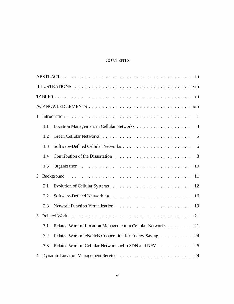
CONTENTS
ABSTRACT . . . . . . . . . . . . . . . . . . . . . . . . . . . . . . . . . . . . . . iii
ILLUSTRATIONS . . . . . . . . . . . . . . . . . . . . . . . . . . . . . . . . . . viii
TABLES . . . . . . . . . . . . . . . . . . . . . . . . . . . . . . . . . . . . . . . . xii
ACKNOWLEDGEMENTS . . . . . . . . . . . . . . . . . . . . . . . . . . . . . . xiii
1 Introduction . . . . . . . . . . . . . . . . . . . . . . . . . . . . . . . . . . . . 1
1.1 Location Management in Cellular Networks . . . . . . . . . . . .. . . . 3
1.2 Green Cellular Networks . . . . . . . . . . . . . . . . . . . . . . . . . . 5
1.3 Software-Defined Cellular Networks . . . . . . . . . . . . . . . . .. . . 6
1.4 Contribution of the Dissertation . . . . . . . . . . . . . . . . . . .. . . 8
1.5 Organization . . . . . . . . . . . . . . . . . . . . . . . . . . . . . . . . . 10
2 Background . . . . . . . . . . . . . . . . . . . . . . . . . . . . . . . . . . . . 11
2.1 Evolution of Cellular Systems . . . . . . . . . . . . . . . . . . . . . .. 12
2.2 Software-Defined Networking . . . . . . . . . . . . . . . . . . . . . . .16
2.3 Network Function Virtualization . . . . . . . . . . . . . . . . . . .. . . 19
3 Related Work . . . . . . . . . . . . . . . . . . . . . . . . . . . . . . . . . . . 21
3.1 Related Work of Location Management in Cellular Networks . . . . . . . 21
3.2 Related Work of eNodeB Cooperation for Energy Saving . . .. . . . . . 24
3.3 Related Work of Cellular Networks with SDN and NFV . . . . . .. . . . 26
4 Dynamic Location Management Service . . . . . . . . . . . . . . . . . .. . . 29
vi

4.1 Virtualized Network Function for Group Location Management . . . . . 29
4.2 Dynamic Profiling Algorithm . . . . . . . . . . . . . . . . . . . . . . . .31
4.3 Group Location Management Procedure . . . . . . . . . . . . . . . .. . 35
4.4 Benefits of Group Location Management . . . . . . . . . . . . . . . .. . 39
4.5 Analysis for Signaling Traffic Overhead Analysis . . . . . .. . . . . . . 44
4.6 Analysis for Average Delay . . . . . . . . . . . . . . . . . . . . . . . . .47
4.7 Evaluations with both Real Data and Data from Mobility Model . . . . . 53
4.8 Summary . . . . . . . . . . . . . . . . . . . . . . . . . . . . . . . . . . 62
5 eNodeB Control with SDN and NVF for Energy Saving . . . . . . . . .. . . . 66
5.1 Siesta Architecture . . . . . . . . . . . . . . . . . . . . . . . . . . . . . 66
5.2 Energy Control with Siesta . . . . . . . . . . . . . . . . . . . . . . . . .69
5.3 Energy-aware Cell Management Algorithm in Siesta . . . . .. . . . . . 73
5.4 Siesta Cell Management . . . . . . . . . . . . . . . . . . . . . . . . . . 79
5.5 Evaluations with LTE Simulator . . . . . . . . . . . . . . . . . . . . .. 86
5.6 Evaluations with Trace-Driven Simulation Results . . . .. . . . . . . . . 90
5.7 Summary . . . . . . . . . . . . . . . . . . . . . . . . . . . . . . . . . . 98
6 Summary . . . . . . . . . . . . . . . . . . . . . . . . . . . . . . . . . . . . . . 100
7 Future Work . . . . . . . . . . . . . . . . . . . . . . . . . . . . . . . . . . . . 103
REFERENCE LIST . . . . . . . . . . . . . . . . . . . . . . . . . . . . . . . . . . 106
VITA . . . . . . . . . . . . . . . . . . . . . . . . . . . . . . . . . . . . . . . . . 116
vii
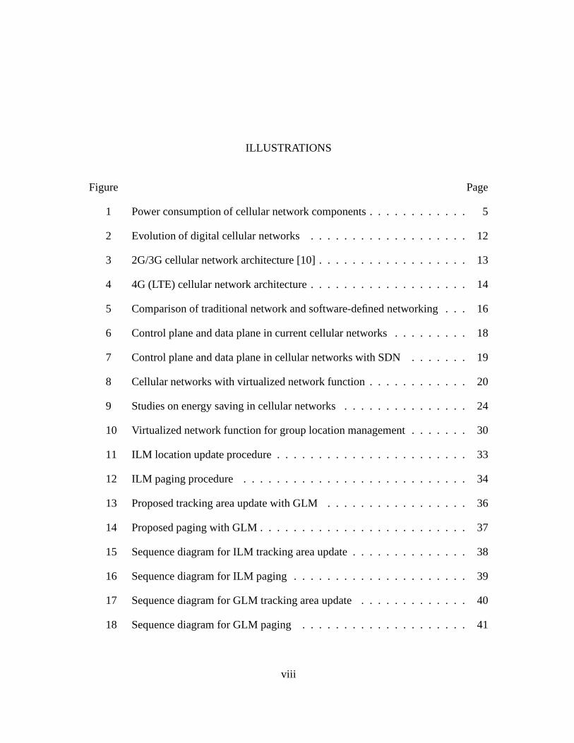
ILLUSTRATIONS
Figure Page
1 Power consumption of cellular network components . . . . . . .. . . . . 5
2 Evolution of digital cellular networks . . . . . . . . . . . . . . . .. . . 12
3 2G/3G cellular network architecture [10] . . . . . . . . . . . . . .. . . . 13
4 4G (LTE) cellular network architecture . . . . . . . . . . . . . . . .. . . 14
5 Comparison of traditional network and software-defined networking . . . 16
6 Control plane and data plane in current cellular networks .. . . . . . . . 18
7 Control plane and data plane in cellular networks with SDN .. . . . . . 19
8 Cellular networks with virtualized network function . . . .. . . . . . . . 20
9 Studies on energy saving in cellular networks . . . . . . . . . . .. . . . 24
10 Virtualized network function for group location management . . . . . . . 30
11 ILM location update procedure . . . . . . . . . . . . . . . . . . . . . . .33
12 ILM paging procedure . . . . . . . . . . . . . . . . . . . . . . . . . . . 34
13 Proposed tracking area update with GLM . . . . . . . . . . . . . . . .. 36
14 Proposed paging with GLM . . . . . . . . . . . . . . . . . . . . . . . . . 37
15 Sequence diagram for ILM tracking area update . . . . . . . . . .. . . . 38
16 Sequence diagram for ILM paging . . . . . . . . . . . . . . . . . . . . . 39
17 Sequence diagram for GLM tracking area update . . . . . . . . . .. . . 40
18 Sequence diagram for GLM paging . . . . . . . . . . . . . . . . . . . . 41
viii

19 Comparison of Total Cost Consumed by ILM and GLM with Varied TA
Overlap Ratio and Increased Residency Time∆ . . . . . . . . . . . . . . 46
20 State transition diagram for paging requests queue in a MME using ILM . 48
21 State transition diagram for paging requests queue in an MME using GLM 50
22 Number of requests in the queue with varied number of groupmembers . 51
23 Number of requests in the queue with varied average call rate . . . . . . 52
24 Data analysis for real trace . . . . . . . . . . . . . . . . . . . . . . . . .54
25 Data analysis for SLAW data . . . . . . . . . . . . . . . . . . . . . . . . 54
26 Comparison of number of tracking area updates (α = 0.9,θ = 0.3,h = 0.75) 55
27 Comparison of the sizes of paging area (α = 0.9,θ = 0.3,h = 0.75) . . . . 55
28 Impact of the GLM parameters on number of tracking area updates (Real
trace) . . . . . . . . . . . . . . . . . . . . . . . . . . . . . . . . . . . . 56
29 Impact of the GLM parameters on the size of paging area (Real trace) . . 56
30 Impact of the GLM parameters on the number of tracking areaupdates
(SLAW data) . . . . . . . . . . . . . . . . . . . . . . . . . . . . . . . . 57
31 Impact of the GLM parameters on the size of paging area (SLAW data) . 58
32 Impact of data characteristic using varied hurst parameters (α = 0.9,θ =
0.5, SLAW data) . . . . . . . . . . . . . . . . . . . . . . . . . . . . . . 59
33 Worst and best cases of paging: Right before and after dynamic profiling . 59
34 Total cost with varied threshold . . . . . . . . . . . . . . . . . . . . .. . 61
35 Total Cost with varied Hurst parameter values (h) . . . . . . . . . . . . . 62
ix
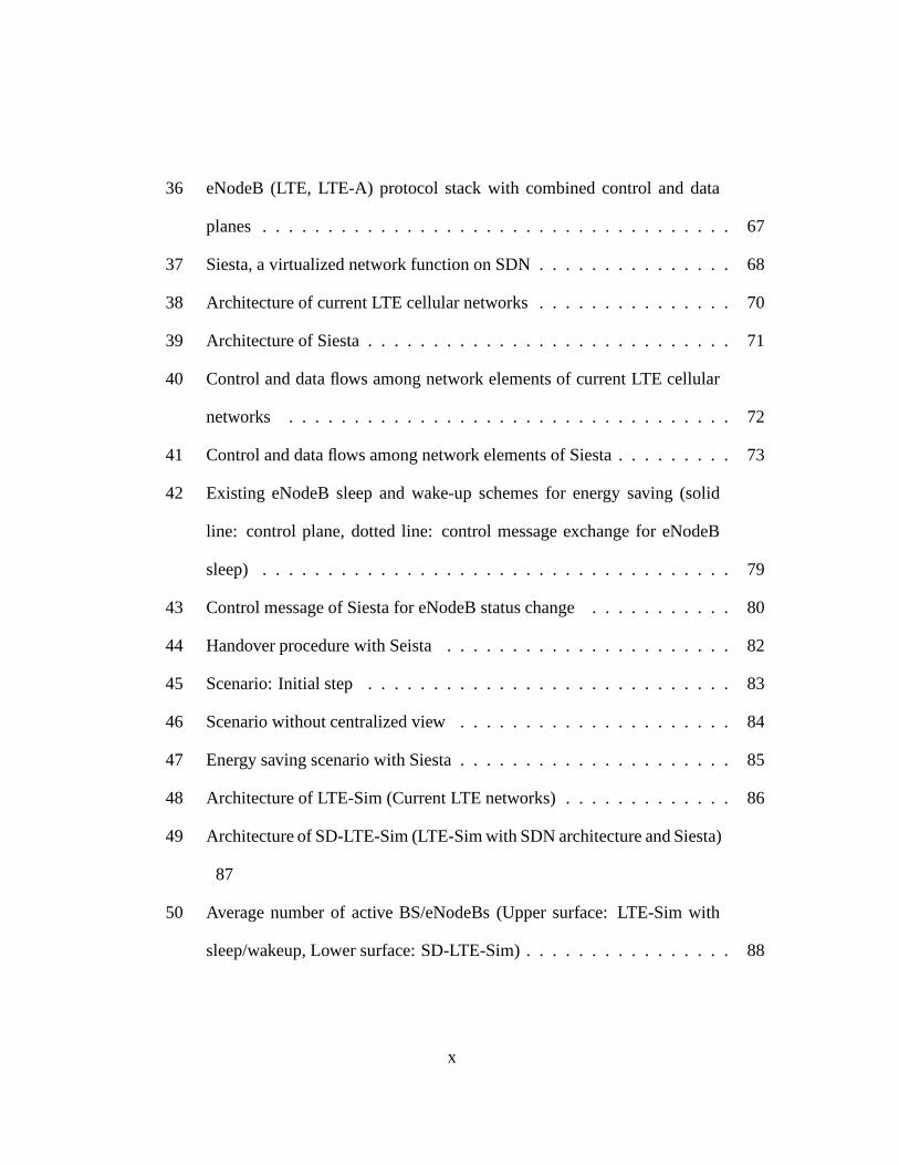
36 eNodeB (LTE, LTE-A) protocol stack with combined controland data
planes . . . . . . . . . . . . . . . . . . . . . . . . . . . . . . . . . . . . 67
37 Siesta, a virtualized network function on SDN . . . . . . . . . .. . . . . 68
38 Architecture of current LTE cellular networks . . . . . . . . .. . . . . . 70
39 Architecture of Siesta . . . . . . . . . . . . . . . . . . . . . . . . . . . . 71
40 Control and data flows among network elements of current LTE cellular
networks . . . . . . . . . . . . . . . . . . . . . . . . . . . . . . . . . . 72
41 Control and data flows among network elements of Siesta . . .. . . . . . 73
42 Existing eNodeB sleep and wake-up schemes for energy saving (solid
line: control plane, dotted line: control message exchangefor eNodeB
sleep) . . . . . . . . . . . . . . . . . . . . . . . . . . . . . . . . . . . . 79
43 Control message of Siesta for eNodeB status change . . . . . .. . . . . 80
44 Handover procedure with Seista . . . . . . . . . . . . . . . . . . . . . .82
45 Scenario: Initial step . . . . . . . . . . . . . . . . . . . . . . . . . . . . 83
46 Scenario without centralized view . . . . . . . . . . . . . . . . . . .. . 84
47 Energy saving scenario with Siesta . . . . . . . . . . . . . . . . . . .. . 85
48 Architecture of LTE-Sim (Current LTE networks) . . . . . . . .. . . . . 86
49 Architecture of SD-LTE-Sim (LTE-Sim with SDN architecture and Siesta)
87
50 Average number of active BS/eNodeBs (Upper surface: LTE-Sim with
sleep/wakeup, Lower surface: SD-LTE-Sim) . . . . . . . . . . . . . .. . 88
x
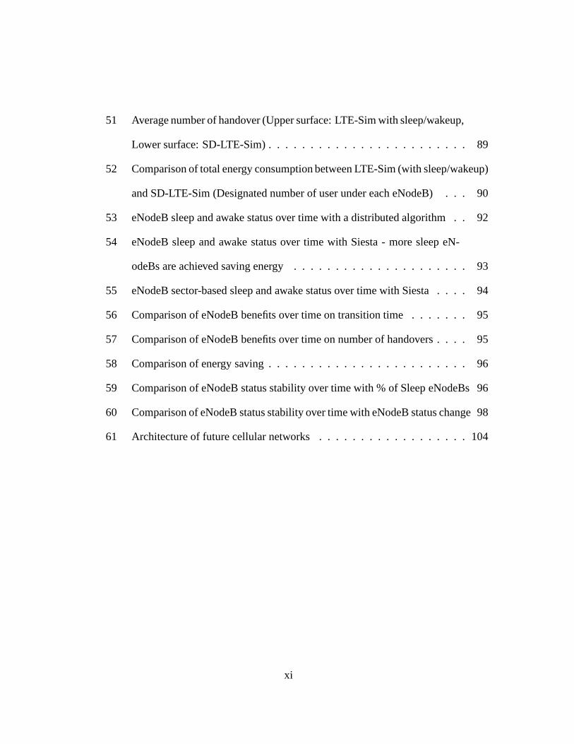
51 Average number of handover (Upper surface: LTE-Sim with sleep/wakeup,
Lower surface: SD-LTE-Sim) . . . . . . . . . . . . . . . . . . . . . . . . 89
52 Comparison of total energy consumption between LTE-Sim (with sleep/wakeup)
and SD-LTE-Sim (Designated number of user under each eNodeB) . . . 90
53 eNodeB sleep and awake status over time with a distributedalgorithm . . 92
54 eNodeB sleep and awake status over time with Siesta - more sleep eN-
odeBs are achieved saving energy . . . . . . . . . . . . . . . . . . . . . 93
55 eNodeB sector-based sleep and awake status over time withSiesta . . . . 94
56 Comparison of eNodeB benefits over time on transition time. . . . . . . 95
57 Comparison of eNodeB benefits over time on number of handovers . . . . 95
58 Comparison of energy saving . . . . . . . . . . . . . . . . . . . . . . . . 96
59 Comparison of eNodeB status stability over time with % of Sleep eNodeBs 96
60 Comparison of eNodeB status stability over time with eNodeB status change 98
61 Architecture of future cellular networks . . . . . . . . . . . . .. . . . . 104
xi
TABLES
Tables Page
1 Explanation of notations for group location management . .. . . . . . . 31
2 Comparison of clustering algorithms . . . . . . . . . . . . . . . . . .. . 32
3 Explanation of additional notations used in analysis . . . .. . . . . . . . 64
4 Data sets used . . . . . . . . . . . . . . . . . . . . . . . . . . . . . . . . 65
5 Impact of threshold on average paging success rate . . . . . . .. . . . . 65
6 Explanation of Notations used in Cell Management Algorithm . . . . . . 74
7 Simulator Setting . . . . . . . . . . . . . . . . . . . . . . . . . . . . . . 87
8 Data sets used (Real traces) . . . . . . . . . . . . . . . . . . . . . . . . . 91
9 Coefficient of variation of the number of sleep eNodeBs . . . .. . . . . . 97
xii

ACKNOWLEDGEMENTS
First of all, I would like to express my deepest gratitude to my advisors Dr. Baek-
Young Choi and Dr. Sejun Song for all their excellent guidance, advice, patience, and
providing me with an excellent atmosphere for doing research. Their great advice and
guidance during my Ph.D. studies contributed to my growth inresearch skills of read-
ing papers critically, discovering ideas, building up projects, and ultimately leading and
managing projects throughout all phases of research.
I would like to thank all of my committee members, Dr. Cory Beard, Dr. Ghu-
lam Chaudhry, and Dr. Masud Chowdhury for all their help and sincere advices when
I approached them with questions. Their comments have helped to clarify and improve
this work. I also would like to thank all the lab mates Daehee Kim, Kaustubh Dhondge,
Xinjie Guan, and Helen Gebre-Amlak for their support and suggestions.
Moreover, I sincerely would like to thank my parents DaehyunShin and Young-
boon Song and my husband’s parents Youngwoo Park and Kyungsook Jang. Also, my
brother Wooshik Shin and brother-in-law Youngjoo Cho. Theywere always supporting
me and encouraging me with their best wishes.
Lastly, but most importantly, I’m grateful to my husband Hyungbae Park and my
two adorable daughters, Katie Park and Claire Park, have always been my happiness and
driving force during my doctoral research. Their love has been and will always be my
momentum to move forward.
CHAPTER 1
INTRODUCTION
Cellular network systems is evolving and provide attractive data and communica-
tion services to fulfill a number of requirements and challenges. The data traffic of cellular
networks is significantly increasing with introduction of new devices such as smartphones
and tablets. In addition, the success of social networking services and associated appli-
cations the data traffic volumes in the networks have exploded during the last few years.
In Ericsson’s report, the data traffic is grown 55 percent between 2014 and 2015. In ad-
dition, the total number of mobile subscription is now around 7.3 billion by adding 87
million new subscriptions. Note that actual number of subscribers is around 4.9 billion,
since many have several subscriptions [30]. Additionally,the global number of base sta-
tions predicted to reach up to 4 million by the end of 2015 to cover increased data traffic.
Therefore, the core network will face congestion due to the increased mobile traffic and
the number of base stations as a solution [52].
With increased data traffic and number of subscription, energy efficiency of cel-
lular networks has received remarkable attention recently. A current estimation indicates
that the Information and Communication Technology (ICT) infrastructure causes 3% of
the world wide electricity consumption and 2% of global CO2 emissions [3].
In order to keep up with the traffic growth, the networks need to optimize the cur-
rent resources and also add new devices/technologies. However, current networks contain
1

complex and inflexible devices. Furthermore, mobile users expect a high quality and
continuous improvement on services. To ensure quality of users’ experience, cellular op-
erators find promising concepts and evolving to make the networks more agile, efficient
and flexible. This can be achieved through virtualized network functions in LTE (Long
Term Evolution) systems [18, 34], and Network Function Virtualization (NFV) architec-
tures are being proposed [11, 57]. NFV addresses the problems of a large and increasing
number of hardware appliances for individual network functions. By virtualizing net-
work functions to commercial off-the-shelf servers, it canreduce capital and operating
expenditures. Additionally, using Software-Defined Network (SDN) principle, redesign
of the Radio Access Network (RAN) and improvement of cellular core networks can be
addressed to obtain network flexibility and manageability.
In this research, we study on location management scheme forgroup applications
to reduce traffic load to the cellular core network. Locationmanagement is one of the
main operation in cellular networks that keeps track of users’ movement to deliver calls
and data. For the group of users who uses the same application, it is possible to reduce
the number of location update with clustering the users based on their geographic loca-
tion. By reducing the number of location update, we can alleviate a well-known bottle
neck problem on the traffic load to the core network. The grouplocation management
scheme is handled as a virtualized network function in cellular network and improves
group application service. Moreover, another virtualizednetwork function for energy ef-
ficient eNodeB control is discussed. By decoupling the functionality of power control of
2

eNodeB, we observe significant improvement on energy consumption in a cellular net-
work. Centralizing the algorithm of cell management, it also greatly simplifies control
over the sleep and awake modes of eNodeB by enabling an agile handover operations.
1.1 Location Management in Cellular Networks
The types of services of cellular networks are also being expanded beyond regular
one-to-one calls. As a major example, Push to Talk over Cellular (PoC) is a service
option for a cellular phone network that allows subscribersto make a call to a group of
users with a single button. PoC service works as a walkie-talkie with an unlimited range.
The connections should be made instantly, with little delay, with all the users in a group.
Currently, only limited versions of the services are available by a few providers [2, 4, 6]
and only for small scale enterprise users. The Open Mobile Alliance [5] is defining PoC
as part of the IP Multimedia Subsystem [81]. Group applications over cellular networks,
such as group audio or video conferencing and stream media broadcasting to a group, are
limited in scale at the moment but will be prevalent in the near future.
The core issue of practical and large scale group call services is the performance.
Here,address an important performance issue for efficient group location management.
Location management is an essential task in cellular mobilenetworks that keeps track
of the movements of individual users and updates a location record in the Home Sub-
scriber Server (HSS). Location management schemes includetwo types of basic opera-
tions, namely i) tracking area update - a report made from a Mobile Node (MN) to the
Mobile Management Entity (MME) when an individual user moves from a Tracking Area
3

(TA) to another TA (Location Area or LA in 3G term); and ii) paging - a message made
by the MME to all cells in a TA to find a callee.
Many location management schemes have been proposed for regular one-to-one
calls. In this paper, we call these approaches Individual Location Management (ILM)
schemes. Such examples include [8, 17, 58, 63, 78] in which there is an attempt to make
the location update decision based on a user’s temporal and spatial movement patterns.
However, the ILM approaches pose a substantial overhead of location management when
they are used for a large number of group members and thus, become infeasible for prac-
tical use.
On the other hand, there are severalcluster-basedlocation management schemes
recommended as well, such as [19,38,45,51] where multiple users’ location updates can
be aggregated when they are clustered within a region.1 However, they are still inherently
designed forone-to-onecalls and can’t be directly applied toone-to-manygroup appli-
cations. This is because, for true PoC services, we can’t mandate that all the MNs of
a group application should belong to a single location area and should exhibit the same
mobility pattern all the time, even though some similarity of group members’ mobility
may be temporarily present. For instance, a part of the groupusers may be located in
different cities. Therefore, a proper location managementscheme forgroup applications
is an imminent need, especially to handle many groups with a large number of members
in a scalable manner.1The authors typically used the word ’group-based’ in those articles. However, we use the word ’cluster-
based’ to refer them, in order to distinguish from the ’group’, a type of applications in this paper.
4
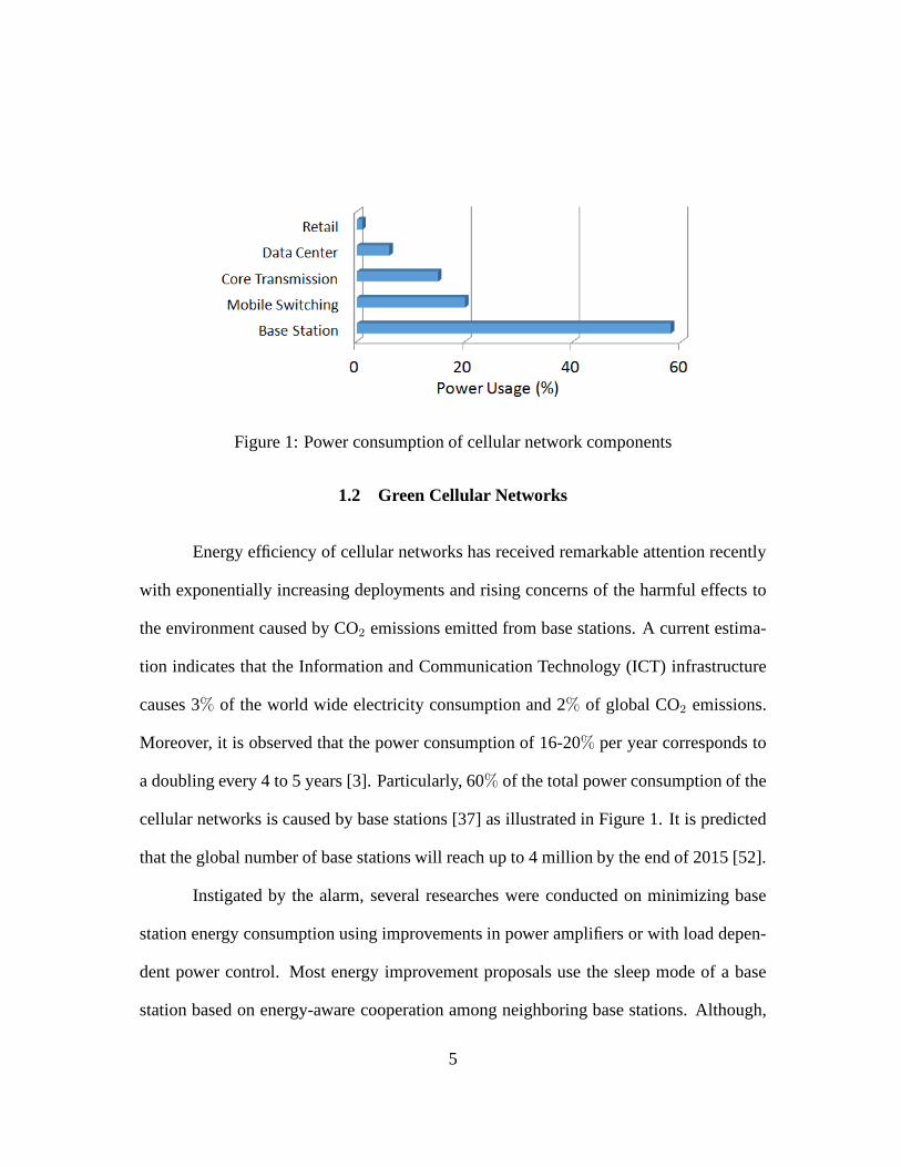
Figure 1: Power consumption of cellular network components
1.2 Green Cellular Networks
Energy efficiency of cellular networks has received remarkable attention recently
with exponentially increasing deployments and rising concerns of the harmful effects to
the environment caused by CO2 emissions emitted from base stations. A current estima-
tion indicates that the Information and Communication Technology (ICT) infrastructure
causes 3% of the world wide electricity consumption and 2% of global CO2 emissions.
Moreover, it is observed that the power consumption of 16-20% per year corresponds to
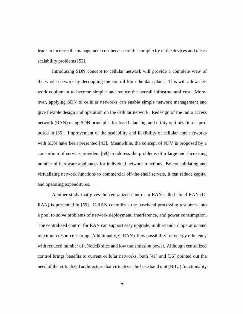
a doubling every 4 to 5 years [3]. Particularly, 60% of the total power consumption of the
cellular networks is caused by base stations [37] as illustrated in Figure 1. It is predicted
that the global number of base stations will reach up to 4 million by the end of 2015 [52].
Instigated by the alarm, several researches were conductedon minimizing base
station energy consumption using improvements in power amplifiers or with load depen-
dent power control. Most energy improvement proposals use the sleep mode of a base
station based on energy-aware cooperation among neighboring base stations. Although,
5
sleep mode can save energy consumption significantly, note that it may cause problems
such as an activation time issue and a ping-pong effect [29].Performance degradation
is experienced during the activation time, and the ping-pong effect that is unnecessary
for on/off oscillations can increase the energy consumption with frequent wake-up pro-
cesses and handover control messages while decreasing the users’ QoS. The problems
intrinsically stem from the sleep mode decision that was made based on myopic informa-
tion of immediate neighboring base stations. The radio access network of LTE or LTE-
Advanced, E-UTRAN (evolved UMTS Terrestrial Radio Access), consists of eNodeBs
that support flexible bandwidth deployments. The eNodeB is acomplex base station (BS)
that communicates with other eNodeBs and core network elements as well. eNodeBs are
responsible for all radio related functions and handover decisions. However, there is no
global, centralized control in the current E-UTRAN.
1.3 Software-Defined Cellular Networks
SDN is an emerging network architecture that allows dynamicand flexible net-
work operations by decoupling the network control plane from the data plane [27]. The
migration of control plan to the logically centralized controller simplifies the network
management and enables new services.
Recently, there has been significant interest in integrating the SDN principles in
current cellular architectures such as 3G Universal MobileTelecommunications System
(UMTS)and 4G LTE [66]. Current cellular network architecture has centralized data flow
and all traffic passes through specialized equipment (e.g.,Packet gateway in LTE). This
6
leads to increase the management cost because of the complexity of the devices and raises
scalability problems [52].
Introducing SDN concept to cellular network will provide a complete view of
the whole network by decoupling the control from the data plane. This will allow net-
work equipment to become simpler and reduce the overall infrastructural cost. More-
over, applying SDN to cellular networks can enable simple network management and
give flexible design and operation on the cellular network. Redesign of the radio access
network (RAN) using SDN principles for load balancing and utility optimization is pro-
posed in [35]. Improvement of the scalability and flexibility of cellular core networks
with SDN have been presented [43]. Meanwhile, the concept ofNFV is proposed by a
consortium of service providers [69] to address the problems of a large and increasing
number of hardware appliances for individual network functions. By consolidating and
virtualizing network functions to commercial off-the-shelf servers, it can reduce capital
and operating expenditures.
Another study that gives the centralized control to RAN called cloud RAN (C-
RAN) is presented in [55]. C-RAN centralizes the baseband processing resources into
a pool to solve problems of network deployment, interference, and power consumption.
The centralized control for RAN can support easy upgrade, multi-standard operation and
maximum resource sharing. Additionally, C-RAN offers possibility for energy efficiency
with reduced number of eNodeB sites and low transmission power. Although centralized
control brings benefits to current cellular networks, both [41] and [36] pointed out the
need of the virtualized architecture that virtualizes the base band unit (BBU) functionality
7
and services in a centralized BBU pool.
1.4 Contribution of the Dissertation
In this dissertation, we focus on two aspects of cellular networks such as location
management and energy saving on SDN and NFV architecture. the main contributions of
this dissertation are as follows.
• We develop an efficient location management scheme forgroup applicationsin cel-
lular networks. We propose a location management architecture that uses a so called
Group Location Management (GLM) and dynamic group profilingof the members’
geographic information. The group location management service can be augmented
as a virtualized network function [69] either for a 3G or 4G cellular network archi-
tecture. The presence of GLM succinctly simplifies the grouplocation management
task and enables cellular network providers to handle a large number of members
and groups. The group profiling algorithm dynamically updates its group members’
location information with clusters of cells or location areas that can be of arbitrary
shapes and sizes. We have validated the efficiency of the proposed scheme with
theoretical analysis as well as extensive experiments. As for the experiments, we
have used both real traces of human movements and synthetic human mobility data.
Note that our scheme is complementary and beneficial to the traditional one-to-one
call location management, but it is also interoperable withit.
• We propose an architecture of a virtualized network function of cell management
8

on a software-defined cellular network, called Siesta (Software-defined energy effi-
cient base station control) for green cellular networks. With the proposed architec-
ture and network-wide information, we then employ a cell management algorithm
that can effectively select a minimal set of eNodeBs that canserve all users without
incurring a ping-pong effect. The ping pong effect is one of the well known prob-
lems in cellular networks that causes unnecessary frequenthandovers. It increases
control messages to the core network and decreases users’ QoS. It also increases the
energy consumption with frequent on-and-off status changes of eNodeBs. Siesta ar-
chitecture reduces the communication overhead among cellular network elements.
Siesta first reduces the control message between network elements due to the move-
ment of the control plane from eNodeB to a Siesta NFV module. Furthermore, the
message exchange necessary for the handover procedure is also decreased com-
pared to the current LTE handover procedure. Through extensive evaluations using
human mobility traces, we show that Siesta cell management scheme achieves sub-
stantial energy savings in a network over an existing state-of-the-art approach. We
also demonstrate the stability of the eNodeB status from various perspectives. Ad-
ditionally, we observed decrease number of eNodeB on and offand handover. Also,
we observe the reduced energy consumption with longer sleepduration.
9
1.5 Organization
The rest of this dissertation is organized as follows. In Chapter 2, we give an
overview on the issues of evolution of cellular networks, SDN, and NFV. Chapter 3 re-
view related work dealing with the location management and energy saving with eNodeB
cooperation. Also, the previous studies on cellular networks with SDN and NFV are dis-
cussed. In Chapters 4 and 5, we identify problems of cellularnetworks in regards to
location management and energy efficiency and propose thoseas a virtualized network
function. Finally, Chapter 6 summarizes and concludes thisdissertation and discusses
future research goals.
10
CHAPTER 2
BACKGROUND
Cellular network systems have revolutionized communication among people and
provide services to make people connected over mobile networks. The First Generation
(1G) refers to analog cellular technologies and has fulfilled the basic mobile voice. The
Second Generation (2G) denoted initial digital systems andhas introduced capacity and
coverage. Currently, Third Generation (3G) and Fourth Generation (4G) technologies is
evolving to fulfill challenges and expectations comes from significantly increased number
of subscribers and a large amount of data over cellular networks [9].
Evolving cellular networks include emerging technologiessuch as SDN and NFV.
SDN an emerging network architecture that allows dynamic and flexible network oper-
ations by decoupling the control plane from the data plane [27]. Introducing SDN to
cellular networks can enable simple network management andgive flexible design and
operation on the cellular networks. Meanwhile, the conceptof NFV is proposed by a
consortium of service providers [69] to address the problems of a large and increasing
number of hardware appliances for individual network functions. By consolidating and
virtualizing network functions to commercial off-the-shelf servers, it can reduce capital
and operating expenditures.
This chapter provides a high level overview of the evolutionof cellular networks
communication. In addition, we also include the objective and efficiency of SDN and
11
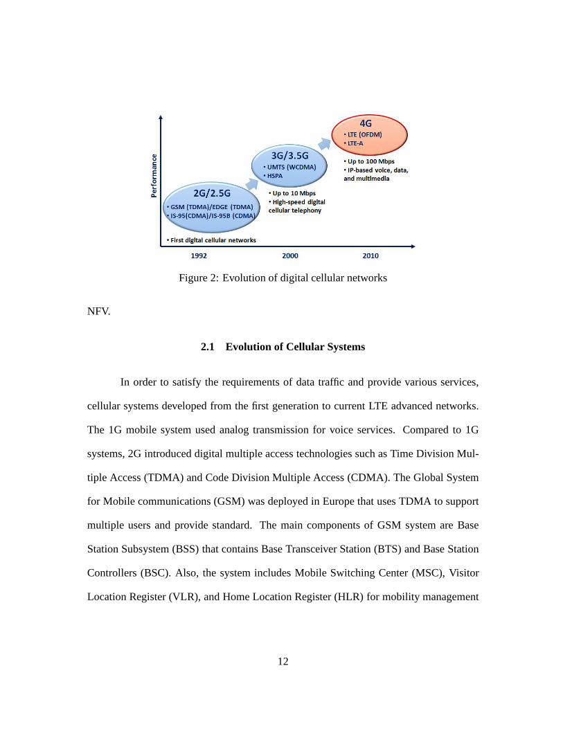
Figure 2: Evolution of digital cellular networks
NFV.
2.1 Evolution of Cellular Systems
In order to satisfy the requirements of data traffic and provide various services,
cellular systems developed from the first generation to current LTE advanced networks.
The 1G mobile system used analog transmission for voice services. Compared to 1G
systems, 2G introduced digital multiple access technologies such as Time Division Mul-
tiple Access (TDMA) and Code Division Multiple Access (CDMA). The Global System
for Mobile communications (GSM) was deployed in Europe thatuses TDMA to support
multiple users and provide standard. The main components ofGSM system are Base
Station Subsystem (BSS) that contains Base Transceiver Station (BTS) and Base Station
Controllers (BSC). Also, the system includes Mobile Switching Center (MSC), Visitor
Location Register (VLR), and Home Location Register (HLR) for mobility management
12

Figure 3: 2G/3G cellular network architecture [10]
of users. As data transfer increased, elements such as Servicing GPRS (SGSN) and Gate-
way GPRS (GGSN) were added. These elements handled the packet data and called
Packet Switched (PS) core network. In the United States, IS-95 that uses CDMA was
deployed.
The 3G was introduced since the need of providing services independent of the
technology platform and whose network design standards aresame globally. The Inter-
national Telecommunication Union (ITU) defined the demandsfor 3G networks with the
IMT-2000 standard and an organization called 3G partnership Project (3GPP) has con-
tinued the work by defining a mobile system. In Europe the system was called UMTS
and WCDMA was used. The main elements were Base Station (BS, or NodeB), Radio
Network Controller (RNC), and SGSN/GGSN. 3G includes wide-area wireless voice tele-
phony and video calls in a mobile environment. Additionally, High Speed Packet Access
(HSPA) data transmission which able to speed up to 14.4 Mbps on the downlink and 5.8
Mbps on the uplink. The summary of evolution of digital cellular networks is presented
in Figure 2 and the architecture of 2G and 3G are shown in Figure 3 [10].
13
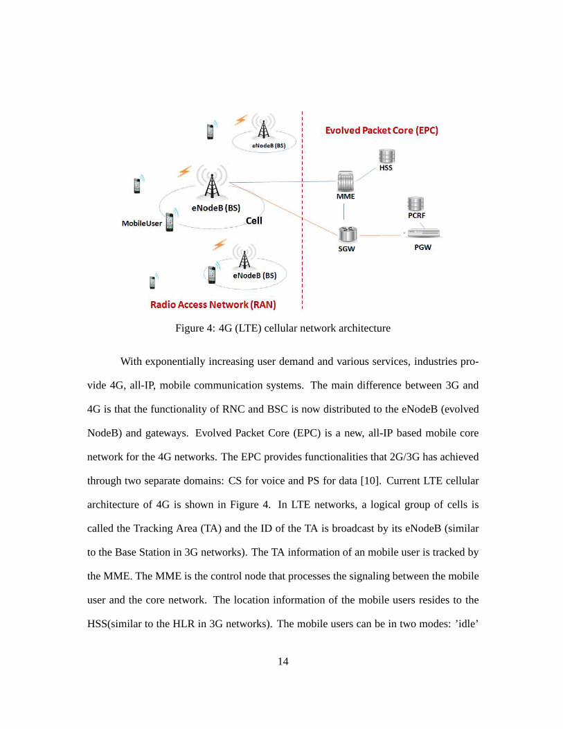
Figure 4: 4G (LTE) cellular network architecture
With exponentially increasing user demand and various services, industries pro-
vide 4G, all-IP, mobile communication systems. The main difference between 3G and
4G is that the functionality of RNC and BSC is now distributedto the eNodeB (evolved
NodeB) and gateways. Evolved Packet Core (EPC) is a new, all-IP based mobile core
network for the 4G networks. The EPC provides functionalities that 2G/3G has achieved
through two separate domains: CS for voice and PS for data [10]. Current LTE cellular
architecture of 4G is shown in Figure 4. In LTE networks, a logical group of cells is
called the Tracking Area (TA) and the ID of the TA is broadcastby its eNodeB (similar
to the Base Station in 3G networks). The TA information of an mobile user is tracked by
the MME. The MME is the control node that processes the signaling between the mobile
user and the core network. The location information of the mobile users resides to the
HSS(similar to the HLR in 3G networks). The mobile users can be in two modes: ’idle’
14

and ’connected.’ The idle mode means that the mobile user does not have a dedicated
connection to the network, but the mobile user listens to thebroadcast channel. A con-
nected mode means that a mobile user has a dedicated connection to the network and has
voice or data transmission.
Although current cellular networks are providing high quality services for their
subscribers, it is challenging to satisfy all the requirements. The limitations of current
networks are listed as below [52].
• Complex network management: Most of the backhaul devices has lack of common
control interfaces. Configuration and policy enforcement requires a proper amount
of effort.
• Inflexibility: Due to the manually intensive service activation and delivery, imple-
mentation of new service takes weeks or months. Also, introducing new services
takes several months or years since the standardization process is a long lasting
process.
• Complex and expensive network devices: The devices in the core network such
as Packet data network Gateway (PGW) are responsible for many significant data
plane functions.
• Higher cost: The operators do not have flexibility to handle the devices from dif-
ferent vendors. This increases the Capital expenditure (CAPEX) and the manual
configuration increases the Operational expenditure (OPEX).
15
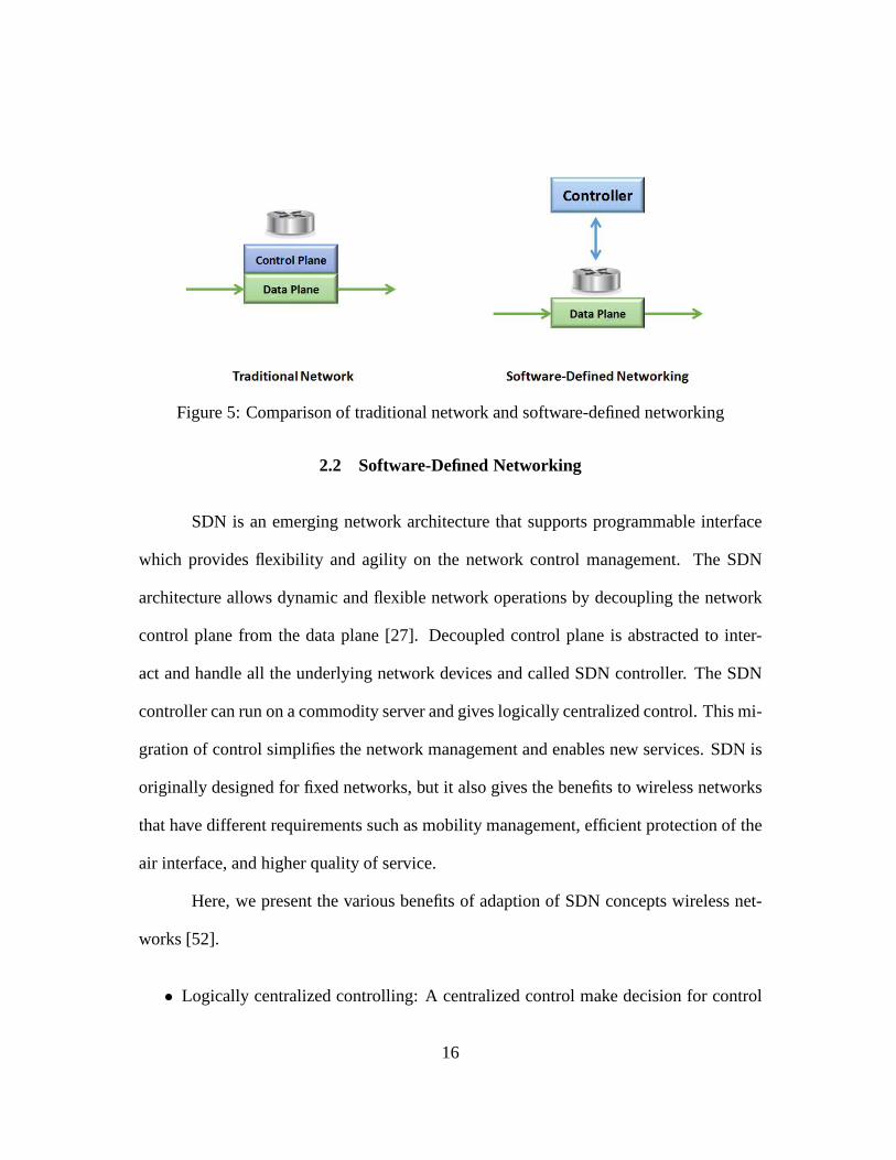
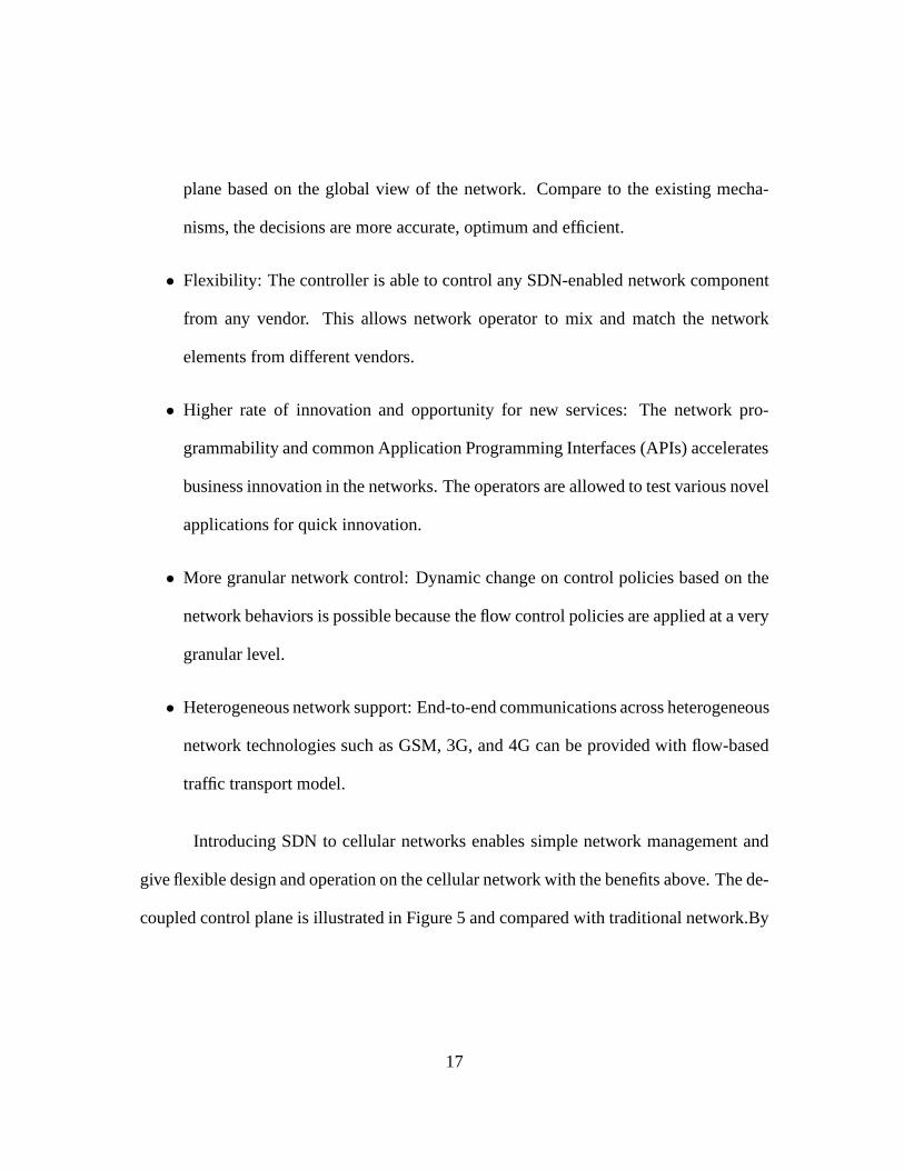
Figure 5: Comparison of traditional network and software-defined networking
2.2 Software-Defined Networking
SDN is an emerging network architecture that supports programmable interface
which provides flexibility and agility on the network control management. The SDN
architecture allows dynamic and flexible network operations by decoupling the network
control plane from the data plane [27]. Decoupled control plane is abstracted to inter-
act and handle all the underlying network devices and calledSDN controller. The SDN
controller can run on a commodity server and gives logicallycentralized control. This mi-
gration of control simplifies the network management and enables new services. SDN is
originally designed for fixed networks, but it also gives thebenefits to wireless networks
that have different requirements such as mobility management, efficient protection of the
air interface, and higher quality of service.
Here, we present the various benefits of adaption of SDN concepts wireless net-
works [52].
• Logically centralized controlling: A centralized controlmake decision for control
16
plane based on the global view of the network. Compare to the existing mecha-
nisms, the decisions are more accurate, optimum and efficient.
• Flexibility: The controller is able to control any SDN-enabled network component
from any vendor. This allows network operator to mix and match the network
elements from different vendors.
• Higher rate of innovation and opportunity for new services:The network pro-
grammability and common Application Programming Interfaces (APIs) accelerates
business innovation in the networks. The operators are allowed to test various novel
applications for quick innovation.
• More granular network control: Dynamic change on control policies based on the
network behaviors is possible because the flow control policies are applied at a very
granular level.
• Heterogeneous network support: End-to-end communications across heterogeneous
network technologies such as GSM, 3G, and 4G can be provided with flow-based
traffic transport model.
Introducing SDN to cellular networks enables simple network management and
give flexible design and operation on the cellular network with the benefits above. The de-
coupled control plane is illustrated in Figure 5 and compared with traditional network.By
17
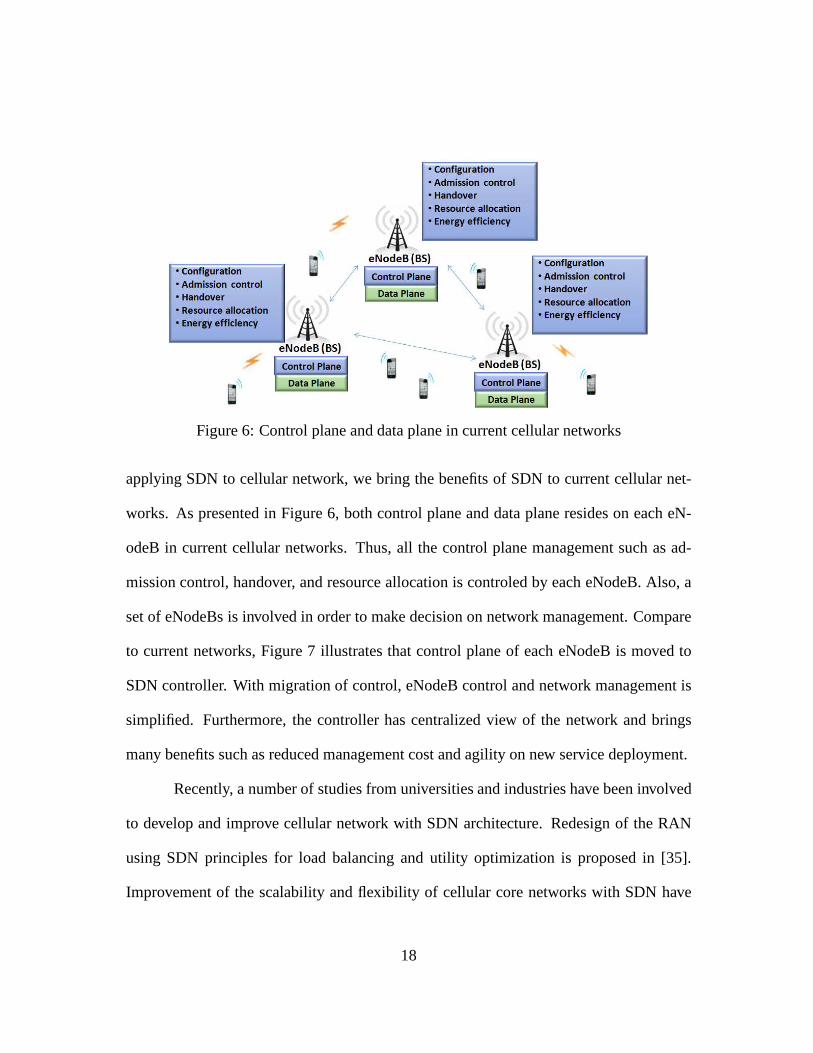
Figure 6: Control plane and data plane in current cellular networks
applying SDN to cellular network, we bring the benefits of SDNto current cellular net-
works. As presented in Figure 6, both control plane and data plane resides on each eN-
odeB in current cellular networks. Thus, all the control plane management such as ad-
mission control, handover, and resource allocation is controled by each eNodeB. Also, a
set of eNodeBs is involved in order to make decision on network management. Compare
to current networks, Figure 7 illustrates that control plane of each eNodeB is moved to
SDN controller. With migration of control, eNodeB control and network management is
simplified. Furthermore, the controller has centralized view of the network and brings
many benefits such as reduced management cost and agility on new service deployment.
Recently, a number of studies from universities and industries have been involved
to develop and improve cellular network with SDN architecture. Redesign of the RAN
using SDN principles for load balancing and utility optimization is proposed in [35].
Improvement of the scalability and flexibility of cellular core networks with SDN have
18

Figure 7: Control plane and data plane in cellular networks with SDN
been presented [43].
2.3 Network Function Virtualization
Meanwhile, the concept of NFV is proposed by a consortium of service providers [69]
to address the problems of a large and increasing number of hardware appliances for indi-
vidual network functions. NFV aims to leverage standard IT virtualization technology to
consolidate many network equipment types onto industry standard high-volume servers,
switches, and storage [32]. By consolidating and virtualizing network functions to com-
mercial off-the-shelf servers, it can reduce capital and operating expenditures. The control
functions in eNodeB that can be virtualized are showned in Figure 8.
Although NFV can be implemented without a SDN being required, the two ap-
proaches can be combined and has potential of greater results. While NFV concentrates
19
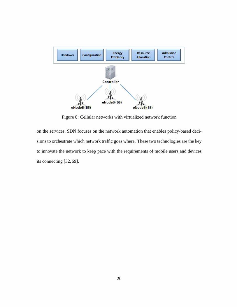
Figure 8: Cellular networks with virtualized network function
on the services, SDN focuses on the network automation that enables policy-based deci-
sions to orchestrate which network traffic goes where. Thesetwo technologies are the key
to innovate the network to keep pace with the requirements ofmobile users and devices
its connecting [32,69].
20
CHAPTER 3
RELATED WORK
Before we discuss our proposed methods, this chapter presents previous works on
individual location management and cluster-based location management. Additionally,
we discuss BS sleep/wakeup schemes and evolving cellular network with SDN and NFV.
Based on the previous works, we point out the problems and insufficient part for the future
cellular networks.
3.1 Related Work of Location Management in Cellular Networks
Location management is necessary in cellular networks in order to keep track
of idle mobile users within the network and forward calls. There are two main tasks in
location management, namely the tracking area update and paging. A tracking area update
is an operation by which a mobile user reports its new location, and paging is initiated by
an eNodeB when an incoming call arrives to find the callee’s location. Once a mobile
user moves to a new TA, a mobile user needs to perform a tracking area update to keep
its location updated in the MME. When the network needs to forward an incoming call
or data to an idle mode mobile user, the MME sends a paging message to all cells in the
mobile users’ last registered TA.
A TA is a group of cells that may be static or dynamic. The number of cells in a TA
21

impacts the signaling traffic of the tracking area updates and paging. The higher computa-
tion and separate data storage for each mobile can be caused by dynamic TAs. However,
it can adapt to the mobility and call pattern of the mobile users resulting in reduced sig-
naling traffic. The static TA has been used in most of the current location management
systems, such as GSM, UMTS, and CDMA2000. In LTE, a mobile node maintains a list
of tracking areas that geographically center around the initial location [50]. Since it is
still only for one-to-one calls, it is not readily made efficient for group communications
as it is. On the other hand, LTE provides a flexible architecture for virtualized network
functions.
Many location management schemes have been proposed for regular one-to-one
calls (thus, using an individual based approach) such as [8,17, 58, 63, 78] that attempt to
make the tracking area update decision based on a user’s temporal and spatial movement
patterns. Defining a TA or LA has been studied extensively to improve the performance
of location management. In [22], a method for selecting the optimal set of cells for each
static TA is proposed. Compared to a static TA, techniques for a dynamic TA are proposed
to dynamically adjust the size and shape of the TA for each individual MN. The TA varies
based on the MNs’ movement patterns and reduces the locationmanagement signaling
traffic overhead. The improved performance of dynamically overlapped TAs is shown
in [24,76,77].
A few techniques using algorithms of the neural network are suggested to add in-
telligence in location management systems. In [71], a profile-based scheme is improved
22
to reduce the location update cost by combining back-propagation algorithms that imple-
ment the learning process. The location prediction methodsare proposed in [61] based on
the users’ movement history and the current state of the user.
Although these approaches would provide improved locationmanagement for
one-to-one calls, they do not exploit the redundancy of the mobility pattern that may
exist in group call applications. Furthermore, they do not address the significant burden
on a server and the control traffic overhead in the HLR or HSS for group calls that lead to
performance degradation.
Cluster-basedlocation management schemes have been proposed in [19, 38, 45,
51]. There are several extra-steps necessary for such cluster-based management ap-
proaches, including cluster establishment, cluster maintenance, and cluster leader selec-
tion. Since only the cluster leader performs a location update on behalf of other cluster
members, this reduces the cost of tracking area updates. Note that cluster-based location
management approaches can only apply to a cluster of users who share a similar mobility
pattern and cannot be directly used for location managementfor group applications. The
mobility pattern of the mobile nodes may not be the same (nor similar) for all mobile
nodes belonging to a group application.
Despite its crucial need, there has been little work to address the issue ofgroup
applicationsin cellular networks. To the best of our knowledge, our work is the first to
study location management for group applications that aimsto reduce the costs of both
tracking area updates and paging. We introduce the concept of a GLM that employs group
23

Figure 9: Studies on energy saving in cellular networks
profile-based location management. GLM architecture is different from group-based pro-
filing architecture, as it is capable of handling profiles of alarge group distributed in a
large area, whereas a group-based scheme can only deal with aprofile within one TA.
3.2 Related Work of eNodeB Cooperation for Energy Saving
The concern on large energy consumption in cellular networks has triggered many
research efforts to reduce eNodeB energy usage. The controlof power in eNodeB is one
of the main methods for energy saving. Limiting power transmission that can reduce both
the amount of interference and energy consumption is discussed in [44]. However, it is
challenging because decreasing the eNodeB transmission power implies a limited impact
on the quality of service. In [72], dynamic power control during a period of low load such
as nighttime is suggested while ensuring full coverage at all times.
24

Another dominant energy saving technique for eNodeB is energy-aware cooper-
ation in eNodeBs. Significant fluctuations of traffic load in cellular networks in space
and time due to users’ behavior is considered for eNodeB cooperation. Limited cell size
adjustment called ”cell-breathing” is suggested in [20]. The mobile user is handed off to
the neighboring cells by reducing a cell size through power control if the cell is under
heavy load or interference. Similarly, a more flexible concept called ”Cell zooming” is
presented in [59]. Cells adjust their size according to the network or traffic situation in
order to balance traffic load and reduce the energy consumption as well. Cell zooming
also allows the eNodeB sleep mode for energy saving, while the neighboring cells can
zoom out and help serve the mobile users cooperatively. For the cell zooming process,
both centralized and distributed algorithms have been developed. More on the eNodeB
sleep mode that is based on traffic load is presented in [40,56,67]. The traffic forecasting
technique for the sleep mode control is based on the daily traffic that was studied in [70].
The quality of service (QoS), which is a significant issue in cellular networks, has been
considered with control of the eNodeB sleep mode. In [29], the eNodeB activation and
deactivation policy maximizes multiple object functions of the QoS and energy consump-
tion, and in [21] each eNodeB estimates the distance of its mobile users and switches off
if there is no degradation of the QoS.
Moreover, concept of Self-Organizing Networks (SON) have been introduced in
3GPP standard that enables network management such as optimization and reconfigura-
tion to heal itself in order to reduce costs and improve network performance and flexi-
bility [13]. The concept of SON can be applied to achieve a large number of objectives.
25

In [68], different use case for SON are discusses such as loadbalancing, cell outage
management, and management of relays and repeaters. The power efficiency and the
performance of SON techniques are investigated in [53,54].
Recently, heterogeneous network deployment based on smaller cells such as mi-
cro, pico, and femto cells has emerged as a promising technique that can possibly reduce
the energy consumption in cellular networks. In [26], the simulation shows that joint de-
ployment of macro and pico cells can reduce the total energy consumption by up to 60%
compared to a network with macro cells only. Additionally, micro eNodeB deployment
and switching on-and-off schemes of macro and micro eNodeBsare presented in [73].
Most previous studies are based on the predictable traffic variation in space and
time such as higher traffic during the daytime and a lower traffic situation at night-
time [40,56,67,70]. Our work is unique in that we exploit information beyond immediate
neighboring cells which is a global view of the network for better decision on energy
saving. To the best of our knowledge, our work is the first to propose an NFV for a cel-
lular network operation. Using SDN architecture, we could employ a cell management
algorithm that yields the best energy efficiency as well as cell stability.
3.3 Related Work of Cellular Networks with SDN and NFV
Current cellular networks supports a number of subscriberswho has frequent mo-
bility and realtime control and services. In addition, various types of services and larger
amount of data over cellular network presents challenges incellular networks. These fea-
tures bring emerging network architecture, SDN and NFV, to evolving cellular network
26
to achieve challenges [12,48].
SDN allows migration of control-related functions to SDN controller and sim-
plifies the network management. Redesign of the RAN using SDNprinciples for load
balancing and utility optimization is proposed in [35]. Improvement of the scalability and
flexibility of cellular core networks with SDN have been presented [43]. NFV is known
as complementary approach to SDN that focuses on optimizingthe network services. The
architecture of virtualized evolved packet core (vEPC) that takes full advantage of NFV
and SDN is presented in [12]. vEPC provides flexibility in network configuration and
management and also accelerates the delivery of new services. Additionally, the concept
of virtualized radio access network (vRAN) that supports centralized radio base station
is introduced in [36]. In thier vRAN architecture, multi-site/multi-standard baseband unit
(MSS-BBU) is introduced for the flexible future cloud-basedRAN structure. The archi-
tecture includes multiple remote radio heads (RRHs) and oneset of MSS-BBUs and a
cluster of RRHs represent a new multi-standard cloud base station. Integration of SDN
and NFV on RAN is suggested in [28]. They pointed out the proposed architecture provies
benefits such as efficient operation, lower power consumption, agile traffic management
and high reliability.
Centralized control to RAN by decoupling BBU and RRH called cloud RAN (C-
RAN) is also presented in [55]. C-RAN centralizes the baseband processing resources
into a pool to solve problems of network deployment, interference, and power consump-
tion. The centralized control for RAN can support easy upgrade, multi-standard operation
27

and maximum resource sharing. Additionally, C-RAN offers possibility for energy effi-
ciency with reduced number of eNodeB sites and low transmission power.
28
CHAPTER 4
DYNAMIC LOCATION MANAGEMENT SERVICE
In this chapter, we describe the proposed group location management scheme. We
first introduce the concept and role of the virtualized network function for group location
management (GLM). GLM manages the information of the group,group members, and
the corresponding tracking areas with cluster profiles. Then, we discuss a dynamic profile-
based TA generation algorithm. Finally, we demonstrate howthe location management
scheme works with the GLM and the dynamic profiles.
4.1 Virtualized Network Function for Group Location Management
In order to accelerate the performance of group applications and alleviate sig-
naling traffic to/from the MME, we introduce a virtualized network function for group
applications as described in Figure 10. GLM is one of the virtualized network functions
(VNFs) that supports group applications.
Group members are the users of the same group applications and therefore, a mes-
sage to a group should be sent to all the members. They are likely, but not necessarily,
to share common activity areas and mobility patterns. Furthermore, each group is pe-
riodically profiled into clusters according to their geographic similarity by our dynamic
profiling algorithm to economize location management costs. Note that the meaning of
’groups’ used here is different from the one used in [19,38,45,51], where groups indicate
29
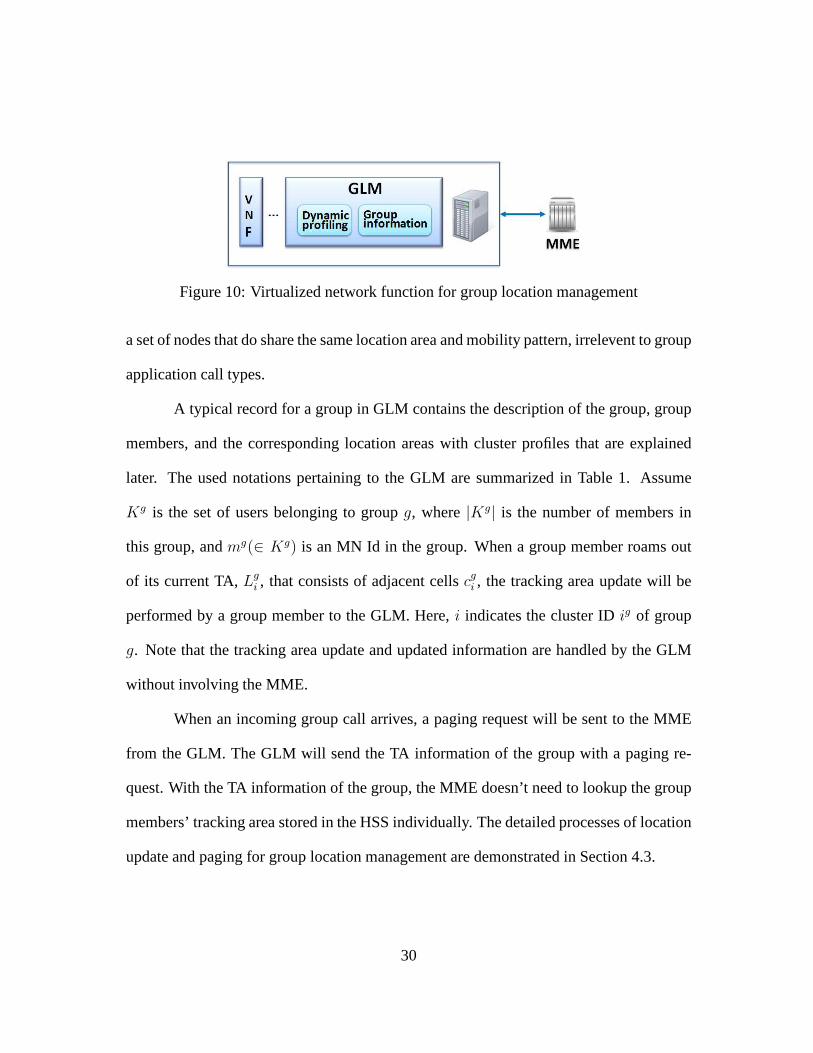
Figure 10: Virtualized network function for group locationmanagement
a set of nodes that do share the same location area and mobility pattern, irrelevent to group
application call types.
A typical record for a group in GLM contains the description of the group, group
members, and the corresponding location areas with clusterprofiles that are explained
later. The used notations pertaining to the GLM are summarized in Table 1. Assume
Kg is the set of users belonging to groupg, where|Kg| is the number of members in
this group, andmg(∈ Kg) is an MN Id in the group. When a group member roams out
of its current TA,Lgi , that consists of adjacent cellscgi , the tracking area update will be
performed by a group member to the GLM. Here,i indicates the cluster IDig of group
g. Note that the tracking area update and updated informationare handled by the GLM
without involving the MME.
When an incoming group call arrives, a paging request will besent to the MME
from the GLM. The GLM will send the TA information of the groupwith a paging re-
quest. With the TA information of the group, the MME doesn’t need to lookup the group
members’ tracking area stored in the HSS individually. The detailed processes of location
update and paging for group location management are demonstrated in Section 4.3.
30
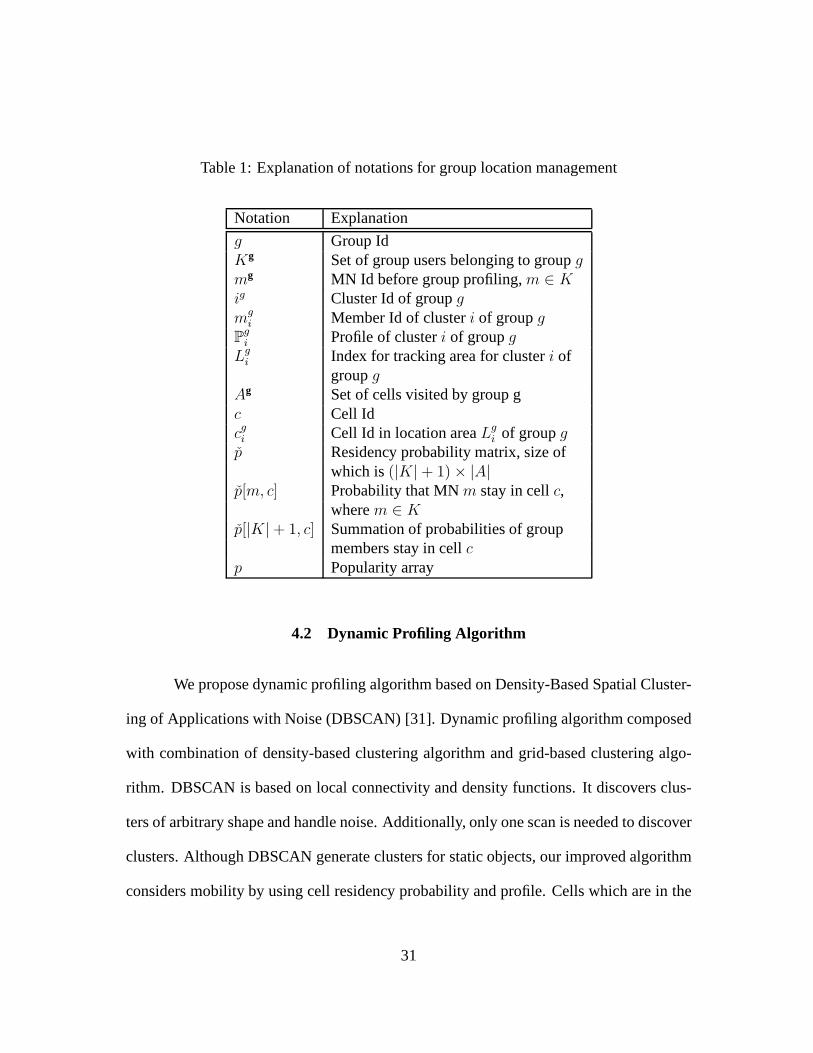
Table 1: Explanation of notations for group location management
Notation Explanation
g Group IdKg Set of group users belonging to groupgmg MN Id before group profiling,m ∈ Kig Cluster Id of groupgmg
i Member Id of clusteri of groupgPgi Profile of clusteri of groupg
Lgi Index for tracking area for clusteri of
groupgAg Set of cells visited by group gc Cell Idcgi Cell Id in location areaLg
i of groupgp̌ Residency probability matrix, size of
which is(|K|+ 1)× |A|p̌[m, c] Probability that MNm stay in cellc,
wherem ∈ Kp̌[|K|+ 1, c] Summation of probabilities of group
members stay in cellcp Popularity array
4.2 Dynamic Profiling Algorithm
We propose dynamic profiling algorithm based on Density-Based Spatial Cluster-
ing of Applications with Noise (DBSCAN) [31]. Dynamic profiling algorithm composed
with combination of density-based clustering algorithm and grid-based clustering algo-
rithm. DBSCAN is based on local connectivity and density functions. It discovers clus-
ters of arbitrary shape and handle noise. Additionally, only one scan is needed to discover
clusters. Although DBSCAN generate clusters for static objects, our improved algorithm
considers mobility by using cell residency probability andprofile. Cells which are in the
31

Table 2: Comparison of clustering algorithms
Density-based clusteringalgorithm (DBSCAN)
Grid-based clustering al-gorithm (STING)
Profile-based cluster algo-rithm (dynamic profilingalgorithm)
One scan Once for each grid One scanArbitrary shape and size Arbitrary shape and size Arbitrary shape and sizeHandle noise Not sensitive to noise Consider noise as a groupNo consideration on mo-bility
No consideration on mo-bility
Consider mobility
Maximum radius of theneighborhood and Mini-mum number of points ofthat point
count, mean, s, min, max,and type of distribution(normal, uniform, etc.)
Cell-based residency prob-ability, weight on profile,and threshold
same LA should be adjacent and minimum number of group members is 1. Furthermore,
we periodically regenerate cluster for mobile users. Table2 shows comparison of exist-
ing clustering algorithms with our suggested algorithm dynamic profiling algorithm. A
conspicuous point of dynamic profiling algorithm is consideration of mobility on users.
In addition, dynamic profiling algorithm can detect a group which has only one member
since noise is also considered as a separate group.
To build clusters, we use member’s movement pattern such as cell residency prob-
ability. Aggregated cells based on the cell residency probability create cluster. The area
which contains members of the same cluster is considered as aone TA. Cell residency
probability is used as an input of dynamic profiling algorithm. In previous group man-
agement schemes, assumption is presented that group is initially defined. In our case,
however, group is not defined. Group members do not know each other or number of
members. In addition, the range and the shape of clusters arevariable. Members have
32
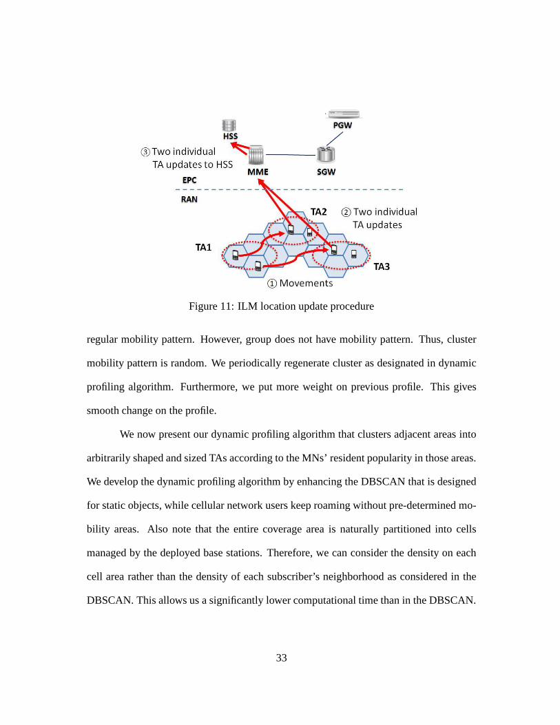
Figure 11: ILM location update procedure
regular mobility pattern. However, group does not have mobility pattern. Thus, cluster
mobility pattern is random. We periodically regenerate cluster as designated in dynamic
profiling algorithm. Furthermore, we put more weight on previous profile. This gives
smooth change on the profile.
We now present our dynamic profiling algorithm that clustersadjacent areas into
arbitrarily shaped and sized TAs according to the MNs’ resident popularity in those areas.
We develop the dynamic profiling algorithm by enhancing the DBSCAN that is designed
for static objects, while cellular network users keep roaming without pre-determined mo-
bility areas. Also note that the entire coverage area is naturally partitioned into cells
managed by the deployed base stations. Therefore, we can consider the density on each
cell area rather than the density of each subscriber’s neighborhood as considered in the
DBSCAN. This allows us a significantly lower computational time than in the DBSCAN.
33
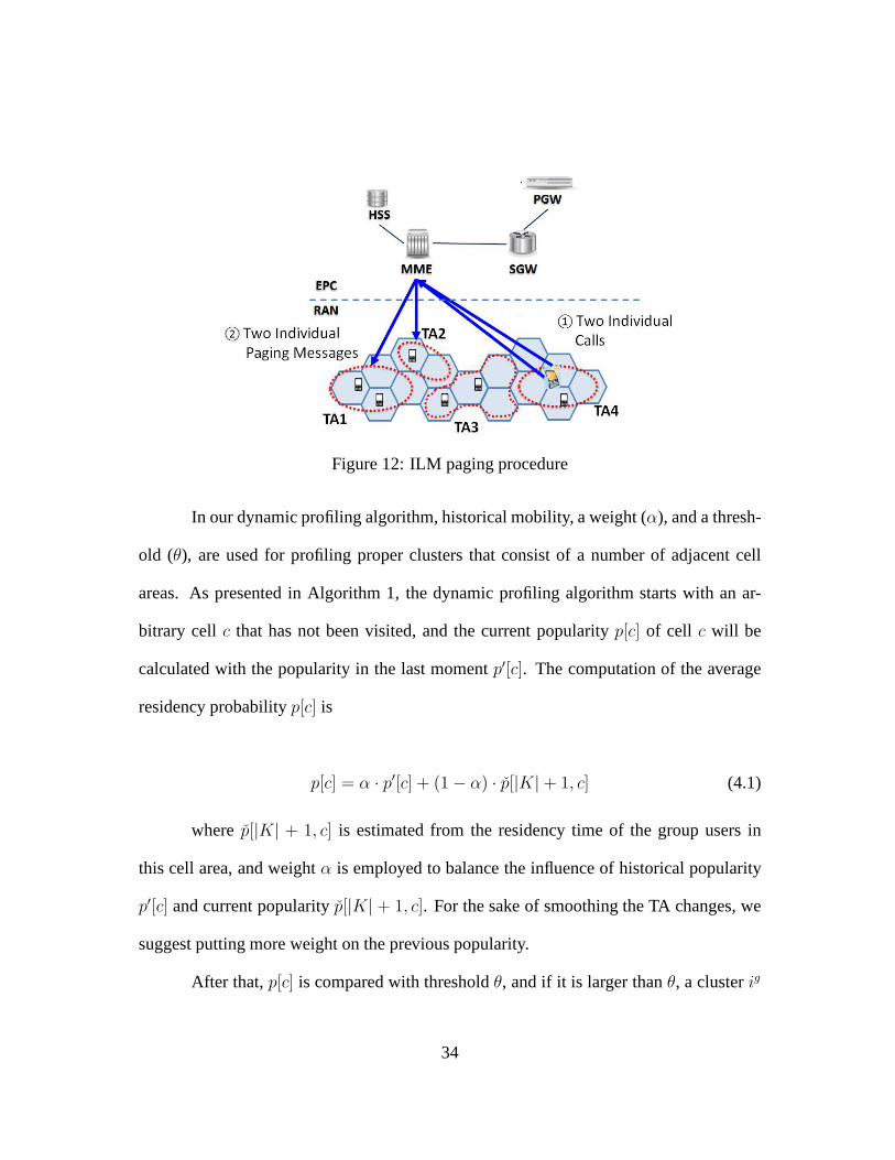
Figure 12: ILM paging procedure
In our dynamic profiling algorithm, historical mobility, a weight (α), and a thresh-
old (θ), are used for profiling proper clusters that consist of a number of adjacent cell
areas. As presented in Algorithm 1, the dynamic profiling algorithm starts with an ar-
bitrary cell c that has not been visited, and the current popularityp[c] of cell c will be
calculated with the popularity in the last momentp′[c]. The computation of the average
residency probabilityp[c] is
p[c] = α · p′[c] + (1− α) · p̌[|K|+ 1, c] (4.1)
where p̌[|K| + 1, c] is estimated from the residency time of the group users in
this cell area, and weightα is employed to balance the influence of historical popularity
p′[c] and current popularity̌p[|K| + 1, c]. For the sake of smoothing the TA changes, we
suggest putting more weight on the previous popularity.
After that,p[c] is compared with thresholdθ, and if it is larger thanθ, a clusterig
34
is formed and all users roaming in this TA belong toig. Furthermore, adjacent neighbors
are queried. If spatial adjacent clusters exist, they will be combined to reduce tracking
area update costs.
The dynamic profiling algorithm requires a little computational time and memory
space. It costsO(|Kg|) time to browse the residency probability for each user, where
|Kg| is the number of users in groupg, thenO(|Ag|) time for traveling every cell area to
cluster the entire coverage area, where|Ag| is the number of cell areas visited by groupg.
Finally, it takesO(1) time to all the neighbors of each cell area, and it maintains amatrix
to record all neighbors for each cell in advance. Consequently, the total time complexity
of the dynamic profiling algorithm isO(max{|Kg|, |Ag|}), where|Kg| is the number of
group members ing and|Ag| is the number of cell areas visited byg. Compared to the
time complexity of the DBSCAN, which isO(|Ag|log|Ag|) using anR∗ tree orO(|Ag|2)
without indexing [31], our algorithm has a smaller time complexity.
On the other hand, the dynamic profiling algorithm occupiesΘ(|Ag|) space for the
neighborhood for each cell area andΘ(|Kg|) space to track each subscriber’s residency
probability. Therefore, the total space complexity of the proposed dynamic profiling al-
gorithm isΘ(max{|Kg|, |Ag|}).
4.3 Group Location Management Procedure
With the assistance of GLM and the dynamic profiling algorithm, the group loca-
tion management can efficiently perform cellular localization with minor changes in cur-
rent cellular networks. The location management of one-to-one calls may not be changed
35
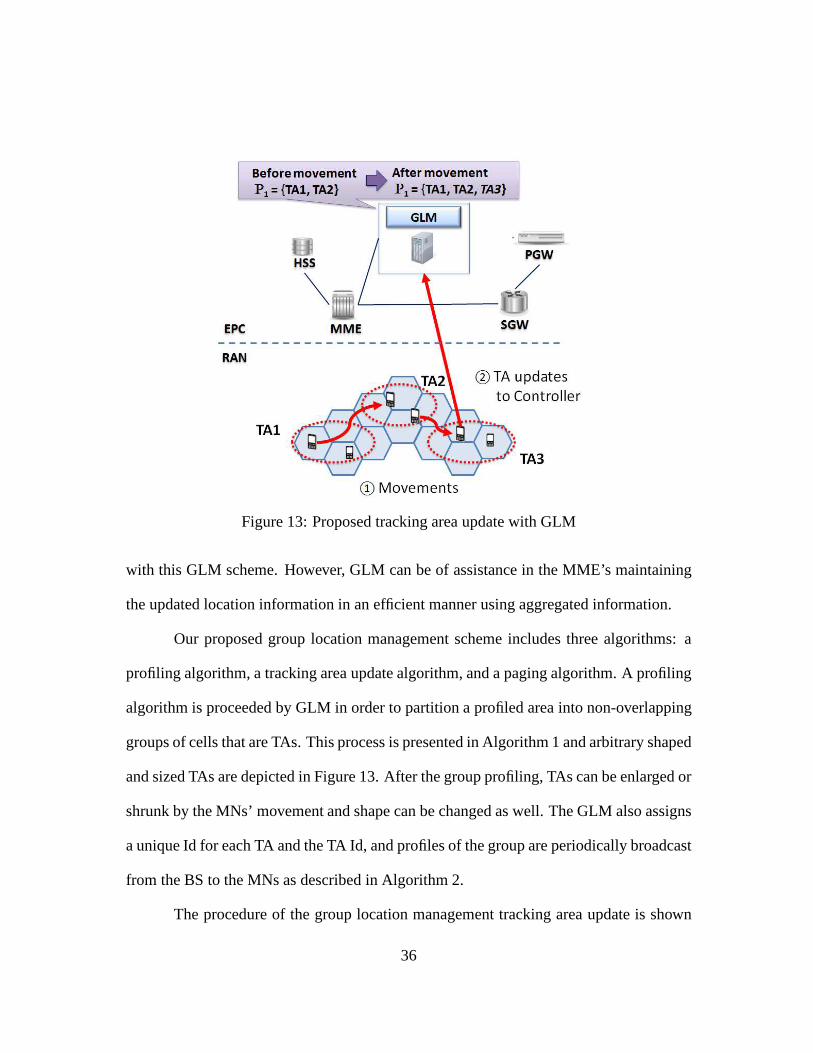
Figure 13: Proposed tracking area update with GLM
with this GLM scheme. However, GLM can be of assistance in theMME’s maintaining
the updated location information in an efficient manner using aggregated information.
Our proposed group location management scheme includes three algorithms: a
profiling algorithm, a tracking area update algorithm, and apaging algorithm. A profiling
algorithm is proceeded by GLM in order to partition a profiledarea into non-overlapping
groups of cells that are TAs. This process is presented in Algorithm 1 and arbitrary shaped
and sized TAs are depicted in Figure 13. After the group profiling, TAs can be enlarged or
shrunk by the MNs’ movement and shape can be changed as well. The GLM also assigns
a unique Id for each TA and the TA Id, and profiles of the group are periodically broadcast
from the BS to the MNs as described in Algorithm 2.
The procedure of the group location management tracking area update is shown
36
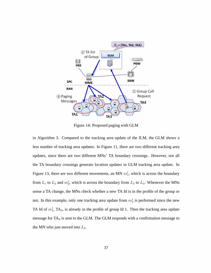
Figure 14: Proposed paging with GLM
in Algorithm 3. Compared to the tracking area update of the ILM, the GLM shows a
less number of tracking area updates. In Figure 11, there aretwo different tracking area
updates, since there are two different MNs’ TA boundary crossings. However, not all
the TA boundary crossings generate location updates in GLM tracking area update. In
Figure 13, there are two different movements, an MNm11, which is across the boundary
from L1 to L2 andm12, which is across the boundary fromL2 to L3. Whenever the MNs
sense a TA change, the MNs check whether a new TA Id is in the profile of the group or
not. In this example, only one tracking area update fromm12 is performed since the new
TA Id of m11, TA2, is already in the profile of group Id 1. Then the tracking areaupdate
message for TA3 is sent to the GLM. The GLM responds with a confirmation message to
the MN who just moved intoL3.
37
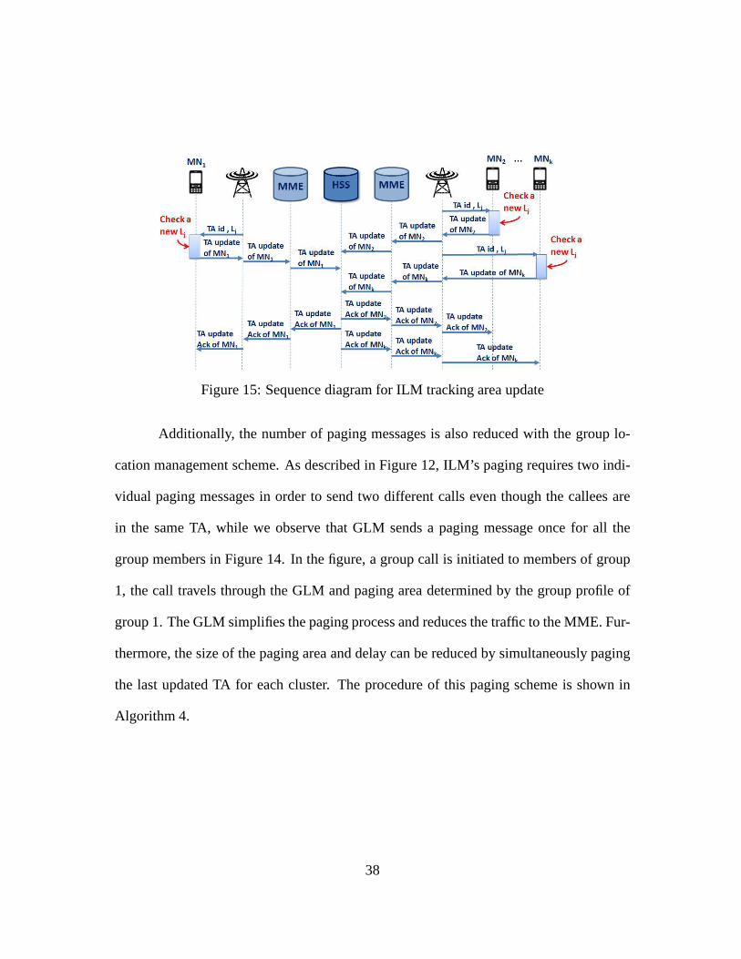
Figure 15: Sequence diagram for ILM tracking area update
Additionally, the number of paging messages is also reducedwith the group lo-
cation management scheme. As described in Figure 12, ILM’s paging requires two indi-
vidual paging messages in order to send two different calls even though the callees are
in the same TA, while we observe that GLM sends a paging message once for all the
group members in Figure 14. In the figure, a group call is initiated to members of group
1, the call travels through the GLM and paging area determined by the group profile of
group 1. The GLM simplifies the paging process and reduces thetraffic to the MME. Fur-
thermore, the size of the paging area and delay can be reducedby simultaneously paging
the last updated TA for each cluster. The procedure of this paging scheme is shown in
Algorithm 4.
38

Figure 16: Sequence diagram for ILM paging
4.4 Benefits of Group Location Management
The benefits of our proposed group location management scheme are two fold.
First, movements outside of a tracking area are reported to the GLM instead of the MME,
which diminishes the overhead of control traffic to/from theMME and the database
lookup operation [46, 64]. This alleviates the performanceproblem of the HLRs and
VLRs in the GSM, UMTS, and CDMA2000 cellular networks [23], and MMEs in the
LTE [50]. Second, the centralized information on the GLM makes it possible to perform
dynamic profiling of a group rather than individuals, and this leads to fewer tracking area
updates and paging costs, as analyzed in Section 4.5.
In order to elucidate how the interactions and order of processes are different
between ILM and GLM, we describe both ILM and GLM with sequence diagrams. While
ILM simply checks the new TA Id with the previous TA Id to make the decision for a
39
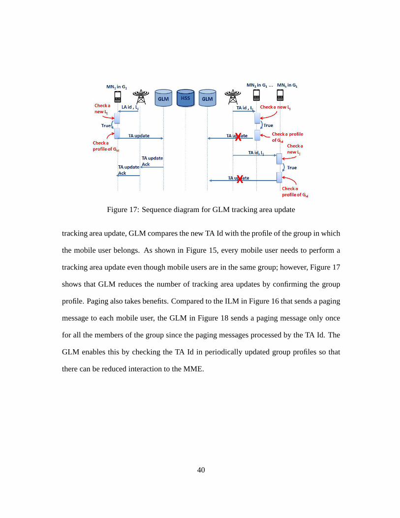
Figure 17: Sequence diagram for GLM tracking area update
tracking area update, GLM compares the new TA Id with the profile of the group in which
the mobile user belongs. As shown in Figure 15, every mobile user needs to perform a
tracking area update even though mobile users are in the samegroup; however, Figure 17
shows that GLM reduces the number of tracking area updates byconfirming the group
profile. Paging also takes benefits. Compared to the ILM in Figure 16 that sends a paging
message to each mobile user, the GLM in Figure 18 sends a paging message only once
for all the members of the group since the paging messages processed by the TA Id. The
GLM enables this by checking the TA Id in periodically updated group profiles so that
there can be reduced interaction to the MME.
40
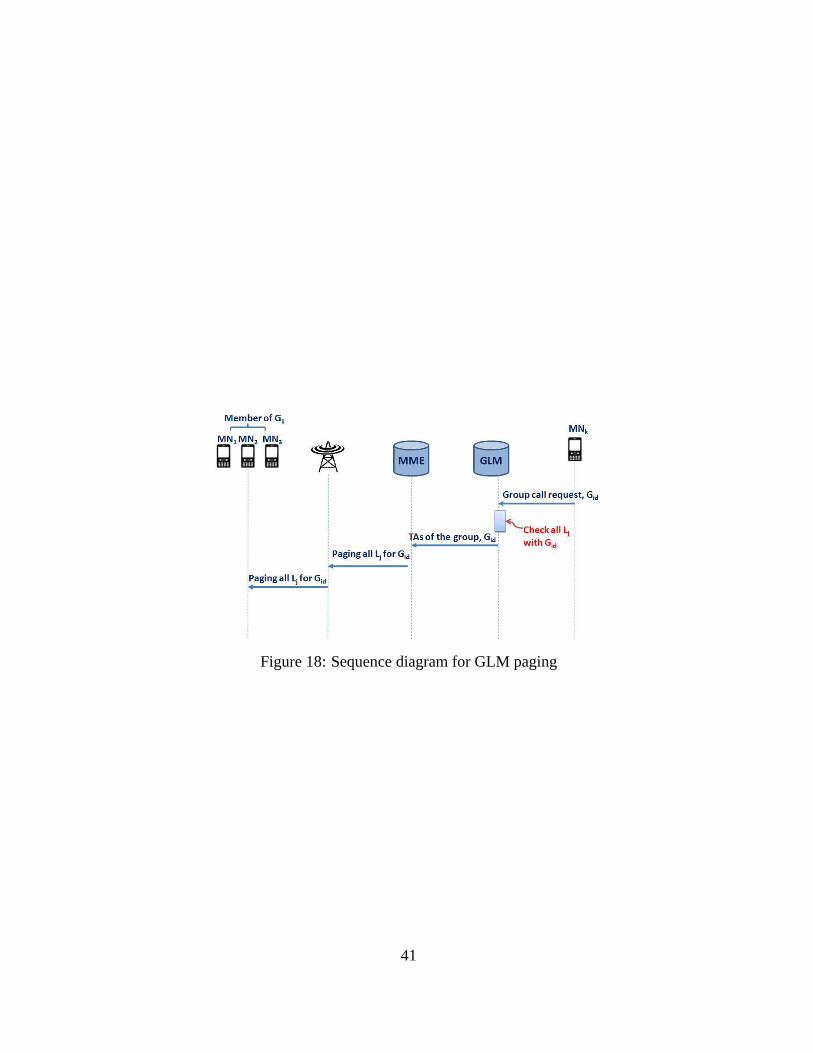
Figure 18: Sequence diagram for GLM paging
41

Algorithm 1 Dynamic profiling algorithm
input Residency probability matrix̌p, popularityarrayp, α, threshold θoutput cell areas in each cluster; group user Ids ineach clusterfor every usermg ∈ Kg
Cumulatep̌[m, c] for cell areac in p̌[(|K|+ 1), c];end forfor each cell areac that has not been visited
markc as visited;calculatep[c] = α× p[c] + (1− α)× p̌[(|K|+ 1), c];if p[c] > θ
construct a new clusterig;put all spacial adjacent cells in a new setnamedNeighborfor each cell areab in Neighbor andp[b] > θ;
if b hasn’t been marked as visitedmarkb that it belongs to clusterig;mark users inb as members ofig;markb asvisited;
elseexpand clusterig with the clusterwhich cell areab belongs to
end ifelse for
end ifend for
42
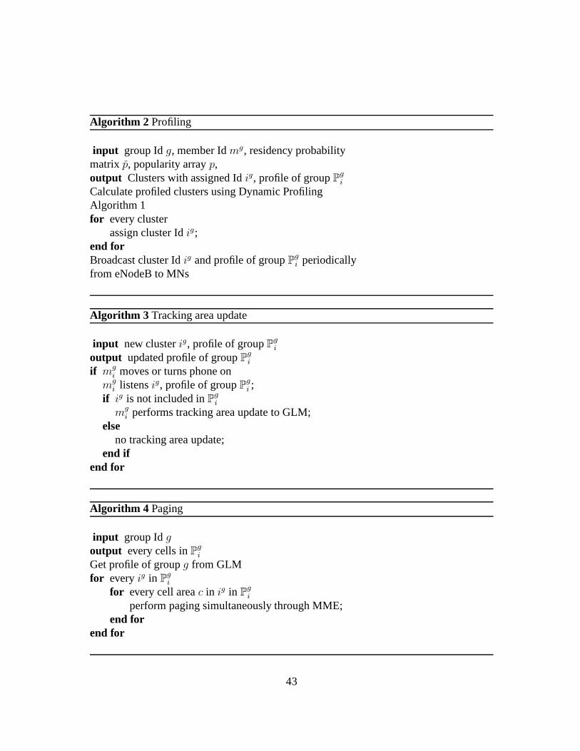
Algorithm 2 Profiling
input group Idg, member Idmg, residency probabilitymatrix p̌, popularity arrayp,output Clusters with assigned Idig, profile of groupPg
i
Calculate profiled clusters using Dynamic ProfilingAlgorithm 1for every cluster
assign cluster Idig;end forBroadcast cluster Idig and profile of groupPg
i periodicallyfrom eNodeB to MNs
Algorithm 3 Tracking area update
input new clusterig, profile of groupPgi
output updated profile of groupPgi
if mgi moves or turns phone on
mgi listensig, profile of groupPg
i ;if ig is not included inPg
i
mgi performs tracking area update to GLM;
elseno tracking area update;
end ifend for
Algorithm 4 Paging
input group Idgoutput every cells inPg
i
Get profile of groupg from GLMfor everyig in P
gi
for every cell areac in ig in Pgi
perform paging simultaneously through MME;end for
end for
43

4.5 Analysis for Signaling Traffic Overhead Analysis
In this section, we illustrate the possible savings of our GLM in signaling traf-
fic overhead and average paging delay by comparing them with atypical ILM through
theoretical analysis. Notations used in this section are summarized in Table 3.
We first show the benefit of our scheme in traffic overhead by analytically compar-
ing the total cost of our GLM with that of a typical ILM. Here, the total cost of a location
management scheme is defined as the signaling traffic overhead that is the summation of
the tracking area update and paging costs. In addition, as widely accepted in previous
research, the tracking area update cost is in proportion to the number of the TA boundary
crossings, while the paging cost is in proportion to the sizeof the TAs.
Suppose the tracking area update cost for each TA boundary crossing isCLU and
the unit cost for paging a single cell TA isCP . Moreover, assume that for an individual
mobile userm, its TA residency timetm, that is the time interval between two bound-
ary crossings, follows Gamma distribution, with density functionftm(·), mean1/λm, and
varianceVm; and the time interval between two group callstg follows exponential distri-
bution with mean1/λg [49]. Let us denotePrm(x) as the probability ofx tracking area
updates for group memberm between two group calls, then we have the expectation for
the total number of tracking area updates/boundary crossings per call arrival using ILM
as
E(x) =∑
m∈K
∑
x∈(0,∞)
x · Prm(x) (4.2)
44

where
Prm(x) =
1− λm
λg[1− f ∗
tm(λg)], x = 0
λm
λg[1− f ∗
tm(λg)]
2[f ∗tm(λg)]
x−1, x > 0(4.3)
f ∗tm(·) is the Laplace-Stieltjes Transform of Gamma random variabletm with mean
1/λm and varianceVm [49], and it can be expressed as:
f ∗tm(s) = (
λmγ
s+ λmγ)γ , where γ =
1
Vmλ2m
(4.4)
Therefore, from Equations (4.2) and (4.3), the expected number of tracking area
updates between two group calls for ILM tracking area updates is
E(K) =∑
m∈K
λm
λg
(4.5)
Meanwhile, the paging cost for ILM is
∑
m∈K
Sm · CP (4.6)
whereSm is the size of the TA that the mobile userm is located in. Therefore, the total
cost per call arrival for ILM is
∑
m∈K
λm
λg
· CLU +∑
m∈K
Sm · CP (4.7)
On the other hand, consider the simplest GLM that the TAs for agroup are deter-
mined by simply combining adjacent TAs for each group member. Therefore, the size of
the group TAs is
⋃
m∈K
Sm (4.8)
45
00.2
0.40.6
0.81
00.2
0.40.6
0.81
0.4
0.6
0.8
1
LA Overlap RatioInc. Residency Time (∆)
Rat
io o
f GLM
Cos
t to
ILM
Cos
t
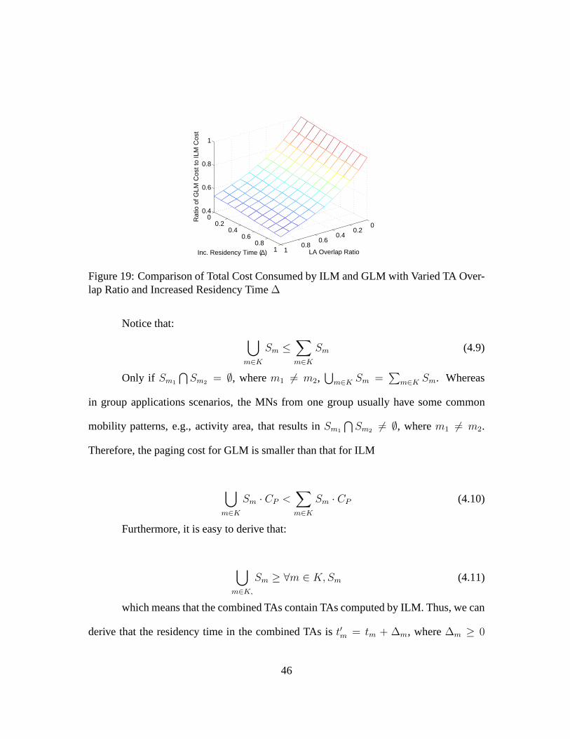
Figure 19: Comparison of Total Cost Consumed by ILM and GLM with Varied TA Over-lap Ratio and Increased Residency Time∆
Notice that:⋃
m∈K
Sm ≤∑
m∈K
Sm (4.9)
Only if Sm1
⋂
Sm2= ∅, wherem1 6= m2,
⋃
m∈K Sm =∑
m∈K Sm. Whereas
in group applications scenarios, the MNs from one group usually have some common
mobility patterns, e.g., activity area, that results inSm1
⋂
Sm26= ∅, wherem1 6= m2.
Therefore, the paging cost for GLM is smaller than that for ILM
⋃
m∈K
Sm · CP <∑
m∈K
Sm · CP (4.10)
Furthermore, it is easy to derive that:
⋃
m∈K,
Sm ≥ ∀m ∈ K,Sm (4.11)
which means that the combined TAs contain TAs computed by ILM. Thus, we can
derive that the residency time in the combined TAs ist′m = tm + ∆m, where∆m ≥ 0
46
is the residency time form in adjacent cellcijl , wherecijl ∈ L′j , andcijl 6∈ Lj . Then the
average residency rate form is
λ′m ≤ λm (4.12)
For the sake of simplicity, assume the residency time for a mobile userm in com-
bined TAs follows Gamma distribution with mean1/λ′m and varianceV ′
m. Then the ex-
pected number of boundary crossings is
E ′(x) =∑
m∈K
∑
x∈(0,∞)
x · Pr′m(x) =∑
m∈K
λ′m
λg
(4.13)
where
Pr′m(x) =
1− λ′
m
λg[1− f ∗
t′m(λg)], x = 0
λ′
m
λg[1− f ∗
t′m(λg)]
2[f ∗t′m(λg)]
x−1, x > 0(4.14)
As λ′m ≤ λm,
E ′(x) ≤ E(x) (4.15)
Assumingλg = 20 min, λm = 5 min, and the ratio ofCLU to CP is 3, the total
cost is compared in Figure 19. As shown in Figure 19, GLM can save up to53% of the
total cost by reducing the expected number of boundary crossings and the paging cost and
an outperform ILM in signaling traffic overhead.
4.6 Analysis for Average Delay
Another benefit of our proposed GLM is that it can reduce the average delay when
group calls come. Intuitively, each group member is paged one by one in consecutive
47
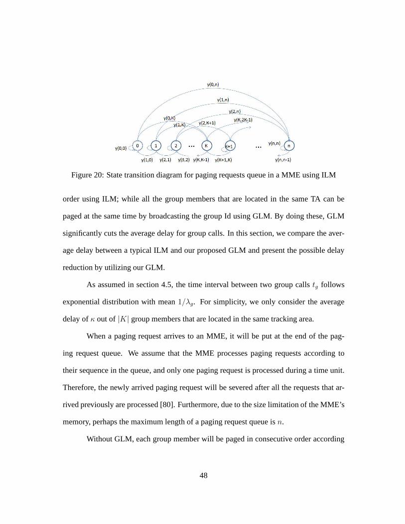
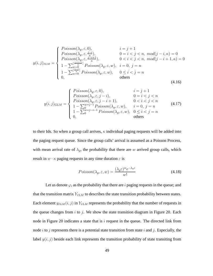
Figure 20: State transition diagram for paging requests queue in a MME using ILM
order using ILM; while all the group members that are locatedin the same TA can be
paged at the same time by broadcasting the group Id using GLM.By doing these, GLM
significantly cuts the average delay for group calls. In thissection, we compare the aver-
age delay between a typical ILM and our proposed GLM and present the possible delay
reduction by utilizing our GLM.
As assumed in section 4.5, the time interval between two group callstg follows
exponential distribution with mean1/λg. For simplicity, we only consider the average
delay ofκ out of |K| group members that are located in the same tracking area.
When a paging request arrives to an MME, it will be put at the end of the pag-
ing request queue. We assume that the MME processes paging requests according to
their sequence in the queue, and only one paging request is processed during a time unit.
Therefore, the newly arrived paging request will be severedafter all the requests that ar-
rived previously are processed [80]. Furthermore, due to the size limitation of the MME’s
memory, perhaps the maximum length of a paging request queueis n.
Without GLM, each group member will be paged in consecutive order according
48
y(i, j)ILM =
Poisson(λg, ε, 0), i = j + 1Poisson(λg, ε,
j−i
κ), 0 = i < j < n, mod(j − i, κ) = 0
Poisson(λg, ε,j−i+1
κ), 0 < i < j < n, mod(j − i+ 1, κ) = 0
1−∑⌈ j−i−1
κ⌉
w=0 Poisson(λg, ε, w), i = 0, j = n
1−∑⌈ j−i
κ⌉
w=0 Poisson(λg, ε, w), 0 ≤ i < j = n0, others
(4.16)
y(i, j)GLM =
Poisson(λg, ε, 0), i = j + 1Poisson(λg, ε, j − i), 0 = i < j < nPoisson(λg, ε, j − i+ 1), 0 < i < j < n
1−∑w=j−i
0 Poisson(λg, ε, w), i = 0, j = n
1−∑w=j−i−1
0 Poisson(λg, ε, w), 0 ≤ i < j = n0, others
(4.17)
to their Ids. So when a group call arrives,κ individual paging requests will be added into
the paging request queue. Since the group calls’ arrival is assumed as a Poisson Process,
with mean arrival rate ofλg, the probability that there arew arrived group calls, which
result inw · κ paging requests in any time durationε is
Poisson(λg, ε, w) =(λgε)
we−λgε
w!(4.18)
Let us denoteϕi as the probability that there arei paging requests in the queue; and
that the transition matrixYILM to describes the state transition probability between states.
Each elementyILM(i, j) in YILM represents the probability that the number of requests in
the queue changes fromi to j. We show the state transition diagram in Figure 20. Each
node in Figure 20 indicates a state that isi request in the queue. The directed link from
nodei to j represents there is a potential state transition from statei andj. Especially, the
labely(i, j) beside each link represents the transition probability of state transiting from
49
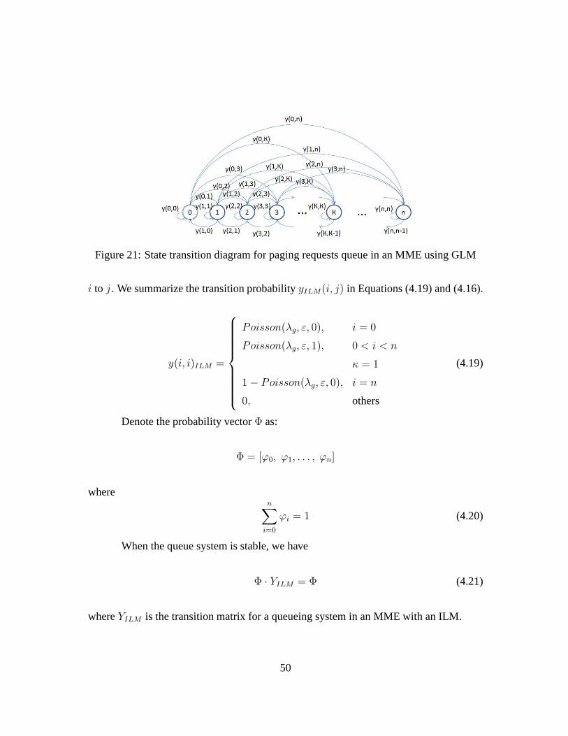
Figure 21: State transition diagram for paging requests queue in an MME using GLM
i to j. We summarize the transition probabilityyILM(i, j) in Equations (4.19) and (4.16).
y(i, i)ILM =
Poisson(λg, ε, 0), i = 0
Poisson(λg, ε, 1), 0 < i < n
κ = 1
1− Poisson(λg, ε, 0), i = n
0, others
(4.19)
Denote the probability vectorΦ as:
Φ = [ϕ0, ϕ1, . . . , ϕn]
wheren
∑
i=0
ϕi = 1 (4.20)
When the queue system is stable, we have
Φ · YILM = Φ (4.21)
whereYILM is the transition matrix for a queueing system in an MME with an ILM.
50
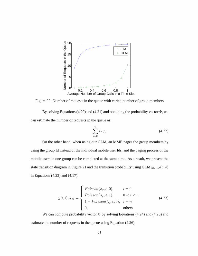
0.2 0.4 0.6 0.8 10
5
10
15
20
Average Number of Group Calls in a Time Slot
Num
ber
of R
eque
sts
in th
e Q
ueue
ILMGLM
Figure 22: Number of requests in the queue with varied numberof group members
By solving Equations (4.20) and (4.21) and obtaining the probability vectorΦ, we
can estimate the number of requests in the queue as:
n∑
i=0
i · ϕi (4.22)
On the other hand, when using our GLM, an MME pages the group members by
using the group Id instead of the individual mobile user Ids,and the paging process of the
mobile users in one group can be completed at the same time. Asa result, we present the
state transition diagram in Figure 21 and the transition probability using GLMyGLM(a, b)
in Equations (4.23) and (4.17).
y(i, i)GLM =
Poisson(λg, ε, 0), i = 0
Poisson(λg, ε, 1), 0 < i < n
1− Poisson(λg, ε, 0), i = n
0, others
(4.23)
We can compute probability vectorΦ by solving Equations (4.24) and (4.25) and
estimate the number of requests in the queue using Equation (4.26).
51
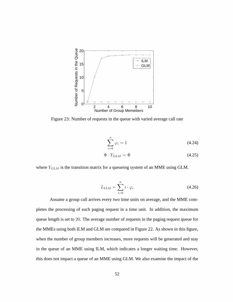
2 4 6 8 100
5
10
15
20
Number of Group Memebers
Num
ber
of R
eque
sts
in th
e Q
ueue
ILMGLM
Figure 23: Number of requests in the queue with varied average call rate
n∑
i=0
ϕi = 1 (4.24)
Φ · YGLM = Φ (4.25)
whereYGLM is the transition matrix for a queueing system of an MME usingGLM.
LILM =
n∑
i=0
i · ϕi (4.26)
Assume a group call arrives every two time units on average, and the MME com-
pletes the processing of each paging request in a time unit. In addition, the maximum
queue length is set to20. The average number of requests in the paging request queue for
the MMEs using both ILM and GLM are compared in Figure 22. As shown in this figure,
when the number of group members increases, more requests will be generated and stay
in the queue of an MME using ILM, which indicates a longer waiting time. However,
this does not impact a queue of an MME using GLM. We also examine the impact of the
52
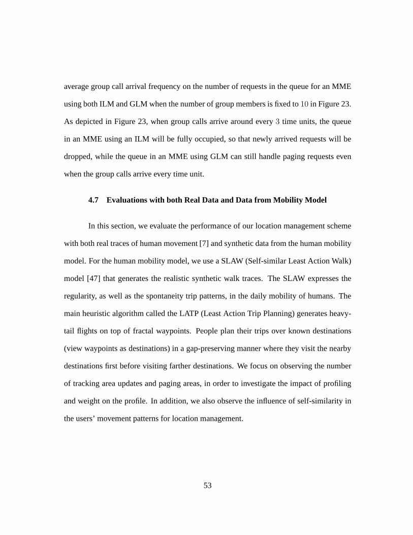
average group call arrival frequency on the number of requests in the queue for an MME
using both ILM and GLM when the number of group members is fixedto 10 in Figure 23.
As depicted in Figure 23, when group calls arrive around every 3 time units, the queue
in an MME using an ILM will be fully occupied, so that newly arrived requests will be
dropped, while the queue in an MME using GLM can still handle paging requests even
when the group calls arrive every time unit.
4.7 Evaluations with both Real Data and Data from Mobility Model
In this section, we evaluate the performance of our locationmanagement scheme
with both real traces of human movement [7] and synthetic data from the human mobility
model. For the human mobility model, we use a SLAW (Self-similar Least Action Walk)
model [47] that generates the realistic synthetic walk traces. The SLAW expresses the
regularity, as well as the spontaneity trip patterns, in thedaily mobility of humans. The
main heuristic algorithm called the LATP (Least Action TripPlanning) generates heavy-
tail flights on top of fractal waypoints. People plan their trips over known destinations
(view waypoints as destinations) in a gap-preserving manner where they visit the nearby
destinations first before visiting farther destinations. We focus on observing the number
of tracking area updates and paging areas, in order to investigate the impact of profiling
and weight on the profile. In addition, we also observe the influence of self-similarity in
the users’ movement patterns for location management.
53

0 10 20 30 400
20
40
60
80
100
Number of Visited Cells
Per
cent
s of
the
Use
rs
0 10 20 30 400
100
200
300
400
Number of Users
Fre
quen
cy o
f Cel
l Cha
nge
(a) Number of cells visited by users in a day (b) Frequency of cell change in a day
Figure 24: Data analysis for real trace
0 10 20 30 400
20
40
60
80
100
Number of Cells
Per
cent
s of
the
user
s
0 20 40 60 80 1000
100
200
300
400
Number of Users
Fre
quen
cy o
f Cel
l Cha
nge
(a) Number of cells visited by users in a day (b) Frequency of cell change in a day
Figure 25: Data analysis for SLAW data
4.7.1 Data sets
The users move around in a 15000 by 15000 meter area that can berepresentative
of a large campus or city. The entire topology consists of 500cells. Detailed settings for
both data are shown in Table 4.
For the SLAW data, we set 5000 waypoints where the users selected several points
54
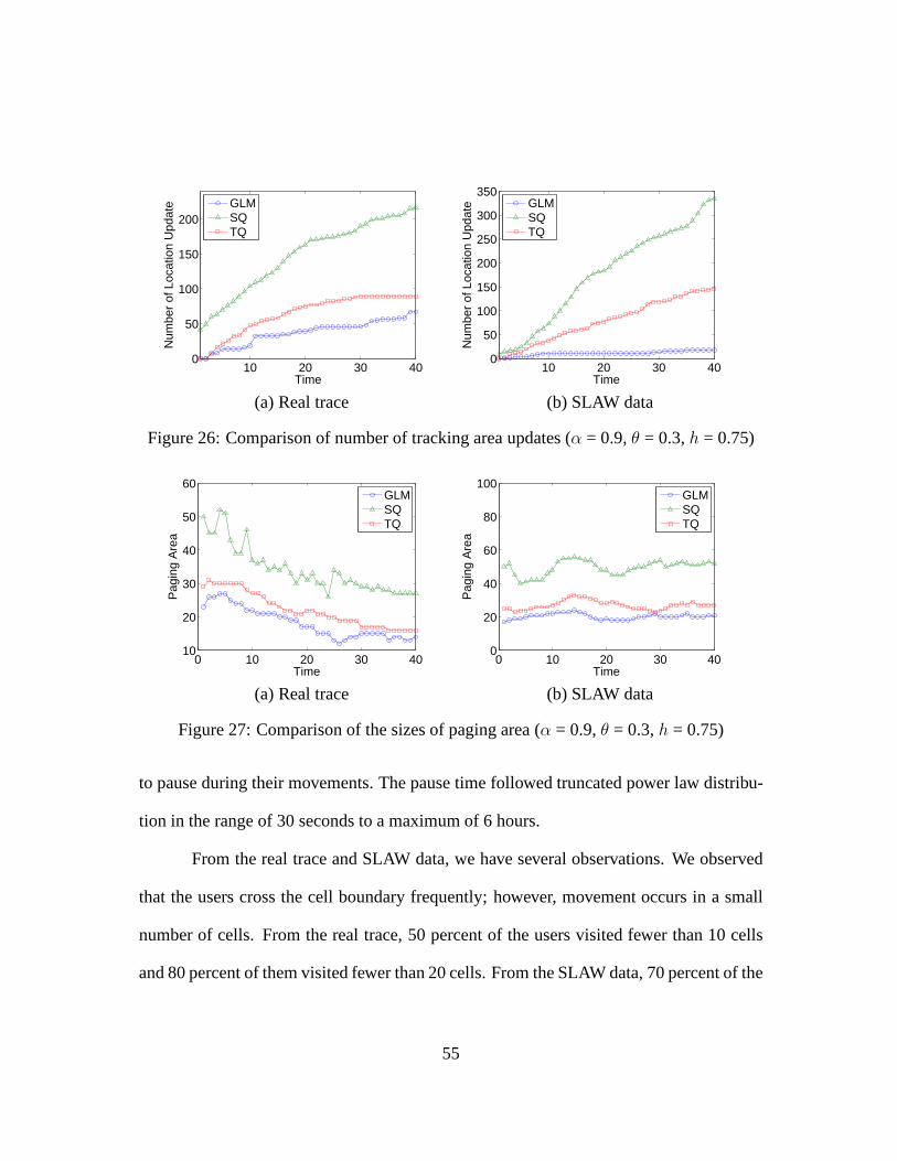
10 20 30 400
50
100
150
200
Time
Num
ber
of L
ocat
ion
Upd
ate
GLMSQTQ
10 20 30 400
50
100
150
200
250
300
350
Time
Num
ber
of L
ocat
ion
Upd
ate
GLMSQTQ
(a) Real trace (b) SLAW data
Figure 26: Comparison of number of tracking area updates (α = 0.9,θ = 0.3,h = 0.75)
0 10 20 30 4010
20
30
40
50
60
Time
Pag
ing
Are
a
GLMSQTQ
0 10 20 30 400
20
40
60
80
100
Time
Pag
ing
Are
a
GLMSQTQ
(a) Real trace (b) SLAW data
Figure 27: Comparison of the sizes of paging area (α = 0.9,θ = 0.3,h = 0.75)
to pause during their movements. The pause time followed truncated power law distribu-
tion in the range of 30 seconds to a maximum of 6 hours.
From the real trace and SLAW data, we have several observations. We observed
that the users cross the cell boundary frequently; however,movement occurs in a small
number of cells. From the real trace, 50 percent of the users visited fewer than 10 cells
and 80 percent of them visited fewer than 20 cells. From the SLAW data, 70 percent of the
55
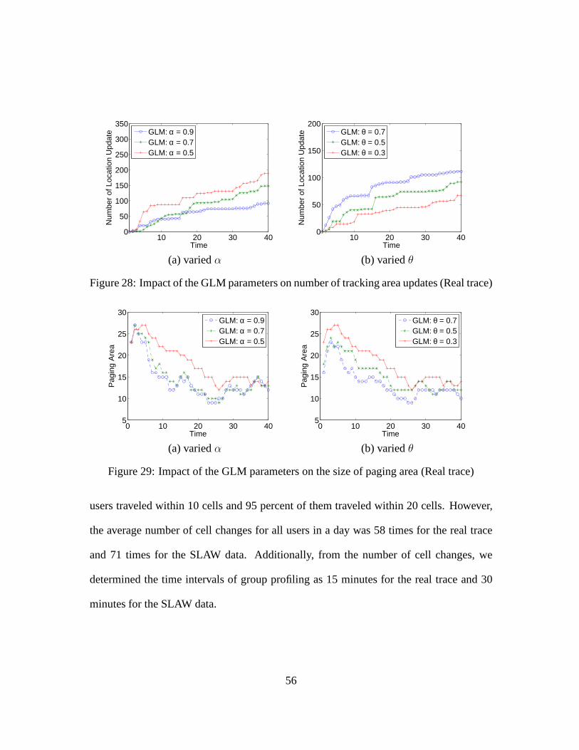
10 20 30 400
50
100
150
200
250
300
350
Time
Num
ber
of L
ocat
ion
Upd
ate
GLM: α = 0.9GLM: α = 0.7GLM: α = 0.5
10 20 30 400
50
100
150
200
Time
Num
ber
of L
ocat
ion
Upd
ate
GLM: θ = 0.7GLM: θ = 0.5GLM: θ = 0.3
(a) variedα (b) variedθ
Figure 28: Impact of the GLM parameters on number of trackingarea updates (Real trace)
0 10 20 30 405
10
15
20
25
30
Time
Pag
ing
Are
a
GLM: α = 0.9GLM: α = 0.7GLM: α = 0.5
0 10 20 30 405
10
15
20
25
30
Time
Pag
ing
Are
a
GLM: θ = 0.7GLM: θ = 0.5GLM: θ = 0.3
(a) variedα (b) variedθ
Figure 29: Impact of the GLM parameters on the size of paging area (Real trace)
users traveled within 10 cells and 95 percent of them traveled within 20 cells. However,
the average number of cell changes for all users in a day was 58times for the real trace
and 71 times for the SLAW data. Additionally, from the numberof cell changes, we
determined the time intervals of group profiling as 15 minutes for the real trace and 30
minutes for the SLAW data.
56
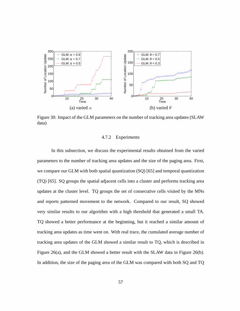
10 20 30 400
50
100
150
200
250
300
Time
Num
ber
of L
ocat
ion
Upd
ate
GLM: α = 0.9GLM: α = 0.7GLM: α = 0.5
10 20 30 400
50
100
150
200
Time
Num
ber
of L
ocat
ion
Upd
ate
GLM: θ = 0.7GLM: θ = 0.5GLM: θ = 0.3
(a) variedα (b) variedθ
Figure 30: Impact of the GLM parameters on the number of tracking area updates (SLAWdata)
4.7.2 Experiments
In this subsection, we discuss the experimental results obtained from the varied
parameters to the number of tracking area updates and the size of the paging area. First,
we compare our GLM with both spatial quantization (SQ) [65] and temporal quantization
(TQ) [65]. SQ groups the spatial adjacent cells into a cluster and performs tracking area
updates at the cluster level. TQ groups the set of consecutive cells visited by the MNs
and reports patterned movement to the network. Compared to our result, SQ showed
very similar results to our algorithm with a high threshold that generated a small TA.
TQ showed a better performance at the beginning, but it reached a similar amount of
tracking area updates as time went on. With real trace, the cumulated average number of
tracking area updates of the GLM showed a similar result to TQ, which is described in
Figure 26(a), and the GLM showed a better result with the SLAWdata in Figure 26(b).
In addition, the size of the paging area of the GLM was compared with both SQ and TQ
57
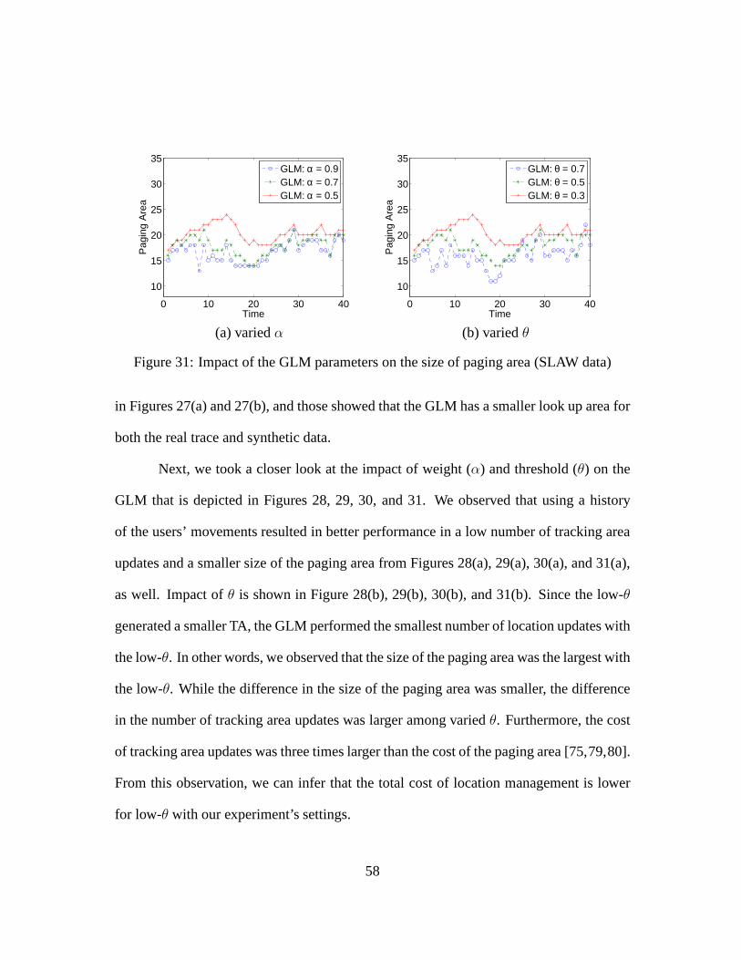
0 10 20 30 40
10
15
20
25
30
35
Time
Pag
ing
Are
a
GLM: α = 0.9GLM: α = 0.7GLM: α = 0.5
0 10 20 30 40
10
15
20
25
30
35
Time
Pag
ing
Are
a
GLM: θ = 0.7GLM: θ = 0.5GLM: θ = 0.3
(a) variedα (b) variedθ
Figure 31: Impact of the GLM parameters on the size of paging area (SLAW data)
in Figures 27(a) and 27(b), and those showed that the GLM has asmaller look up area for
both the real trace and synthetic data.
Next, we took a closer look at the impact of weight (α) and threshold (θ) on the
GLM that is depicted in Figures 28, 29, 30, and 31. We observedthat using a history
of the users’ movements resulted in better performance in a low number of tracking area
updates and a smaller size of the paging area from Figures 28(a), 29(a), 30(a), and 31(a),
as well. Impact ofθ is shown in Figure 28(b), 29(b), 30(b), and 31(b). Since the low-θ
generated a smaller TA, the GLM performed the smallest number of location updates with
the low-θ. In other words, we observed that the size of the paging area was the largest with
the low-θ. While the difference in the size of the paging area was smaller, the difference
in the number of tracking area updates was larger among varied θ. Furthermore, the cost
of tracking area updates was three times larger than the costof the paging area [75,79,80].
From this observation, we can infer that the total cost of location management is lower
for low-θ with our experiment’s settings.
58
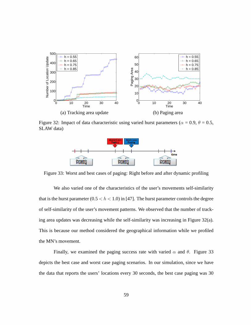
0 10 20 30 400
100
200
300
400
500
Time
Num
ber
of L
ocat
ion
Upd
ate
h = 0.55h = 0.65h = 0.75h = 0.85
0 10 20 30 400
10
20
30
40
50
60
Time
Pag
ing
Are
a
h = 0.55h = 0.65h = 0.75h = 0.85
(a) Tracking area update (b) Paging area
Figure 32: Impact of data characteristic using varied hurstparameters (α = 0.9,θ = 0.5,SLAW data)
Figure 33: Worst and best cases of paging: Right before and after dynamic profiling
We also varied one of the characteristics of the user’s movements self-similarity
that is the hurst parameter (0.5< h< 1.0) in [47]. The hurst parameter controls the degree
of self-similarity of the user’s movement patterns. We observed that the number of track-
ing area updates was decreasing while the self-similarity was increasing in Figure 32(a).
This is because our method considered the geographical information while we profiled
the MN’s movement.
Finally, we examined the paging success rate with variedα and θ. Figure 33
depicts the best case and worst case paging scenarios. In oursimulation, since we have
the data that reports the users’ locations every 30 seconds,the best case paging was 30
59
seconds later than the cluster regeneration and the worst case paging was 30 seconds
before the cluster regeneration. Table 5 shows the average paging success rate for each
threshold. We observedθ between 0.3 and 0.5 showed a high success rate. Also, we
observed that the paging success rate was higher while we used higherα in order to give
more incentive on the history of the users’ movement patterns.
4.7.3 Cost evaluation for location management
In this section, we evaluate the location management cost that consists of two
components: the tracking area update cost and paging cost. Also, we observe the effect
of the hurst parameter that can vary the self-similarity of the mobile users’ movement
pattern on the cost of location management.
In order to study the location management cost and understand factors that can
impact the cost, we used the average number of tracking area updates and the size of
the paging area that we obtained in section 4.7.2. From the result of section 4.7.2, we
already know that both the tracking area update cost and paging cost can be effected by
the size of the TAs and the self-similarity of the mobile user’s movement. The mobile
user’s movement can be classified as below.
• M cellm : average number of movements of userm across cell boundary
• MTAm : average number of movements of userm across the TA boundary
• MPm: average number of movements of userm across the TA boundary within a
group profile
60
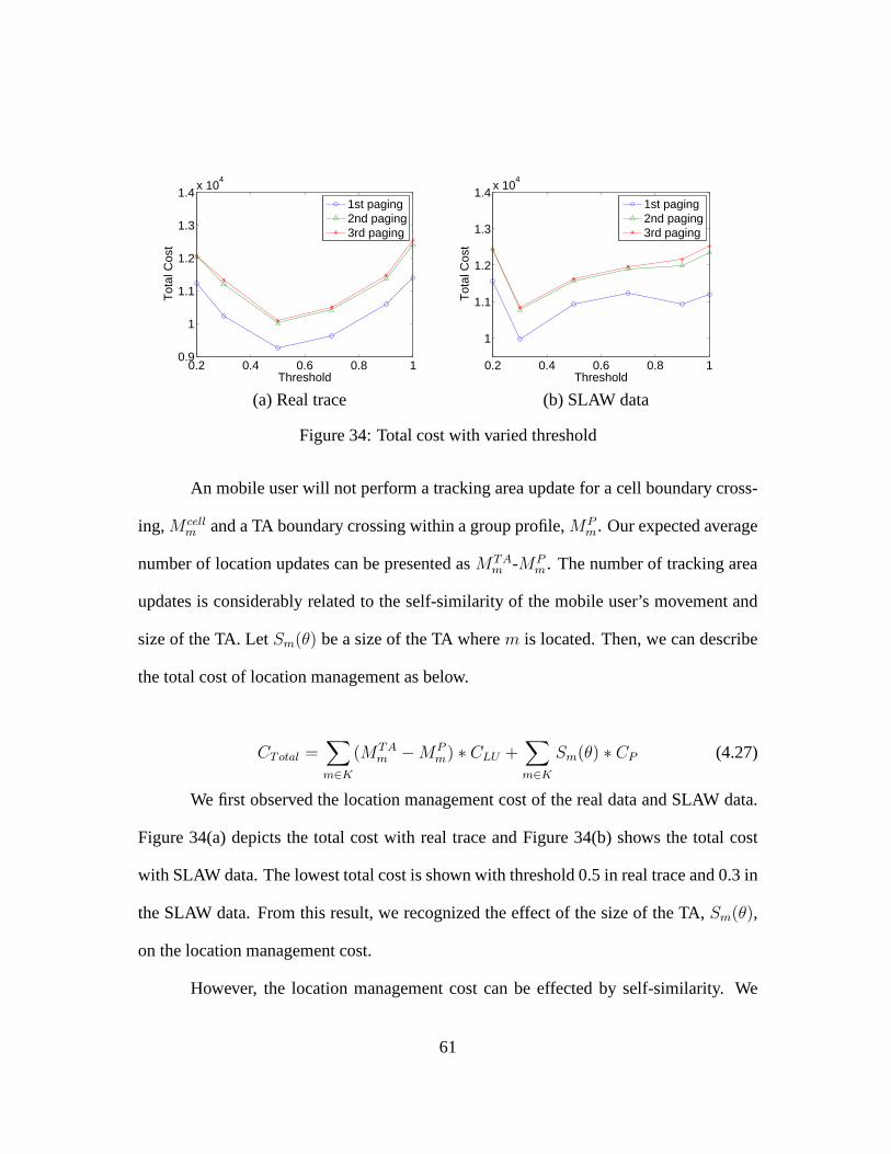
0.2 0.4 0.6 0.8 10.9
1
1.1
1.2
1.3
1.4x 10
4
Threshold
Tot
al C
ost
1st paging2nd paging3rd paging
0.2 0.4 0.6 0.8 1
1
1.1
1.2
1.3
1.4x 10
4
Threshold
Tot
al C
ost
1st paging2nd paging3rd paging
(a) Real trace (b) SLAW data
Figure 34: Total cost with varied threshold
An mobile user will not perform a tracking area update for a cell boundary cross-
ing,M cellm and a TA boundary crossing within a group profile,MP
m. Our expected average
number of location updates can be presented asMTAm -MP
m. The number of tracking area
updates is considerably related to the self-similarity of the mobile user’s movement and
size of the TA. LetSm(θ) be a size of the TA wherem is located. Then, we can describe
the total cost of location management as below.
CTotal =∑
m∈K
(MTAm −MP
m) ∗ CLU +∑
m∈K
Sm(θ) ∗ CP (4.27)
We first observed the location management cost of the real data and SLAW data.
Figure 34(a) depicts the total cost with real trace and Figure 34(b) shows the total cost
with SLAW data. The lowest total cost is shown with threshold0.5 in real trace and 0.3 in
the SLAW data. From this result, we recognized the effect of the size of the TA,Sm(θ),
on the location management cost.
However, the location management cost can be effected by self-similarity. We
61
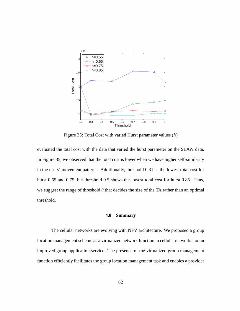
0.2 0.3 0.4 0.5 0.6 0.7 0.8 0.9 1
1
1.5
2
2.5
3
x 104
Threshold
Tot
al C
ost
h=0.55h=0.65h=0.75h=0.85
Figure 35: Total Cost with varied Hurst parameter values (h)
evaluated the total cost with the data that varied the hurst parameter on the SLAW data.
In Figure 35, we observed that the total cost is lower when we have higher self-similarity
in the users’ movement patterns. Additionally, threshold 0.3 has the lowest total cost for
hurst 0.65 and 0.75, but threshold 0.5 shows the lowest totalcost for hurst 0.85. Thus,
we suggest the range of thresholdθ that decides the size of the TA rather than an optimal
threshold.
4.8 Summary
The cellular networks are evolving with NFV architecture. We proposed a group
location management scheme as a virtualized network function in cellular networks for an
improved group application service. The presence of the virtualized group management
function efficiently facilitates the group location management task and enables a provider
62
to handle a large number of members and groups that otherwisewould be impossible
in practice.The group profiling algorithm dynamically updates its group members’ loca-
tions information with clusters of cells or tracking areas that can be of arbitrary shapes.
We validated the efficiency of the proposed scheme with theoretical analyses as well as
experiments. The theoretical analyses showed the total signaling traffic cost and signif-
icant reduction of average delay. As for the experiments, weused both real traces of
human movements and synthetic human mobility data for the tracking area update and
paging costs. Moreover, we investigated the impact of the parameter that describes the
self-similarity of the human walk and suggested the range ofthe threshold that decides
the size of the TA. To the best of our knowledge, our work is thefirst to address the issue
of location management for group applications.
There are related challenges that need to be addressed in thefuture. The benefit
of the proposed architecture can be further substantiated with the development and eval-
uation of a group call signaling protocol that we plan to address in the near future. Also,
there is no human group mobility model at the moment, and it would be useful for eval-
uations of schemes for group applications. That will also enable us to perform a detailed
theoretical analysis of the proposed group location management scheme.
63
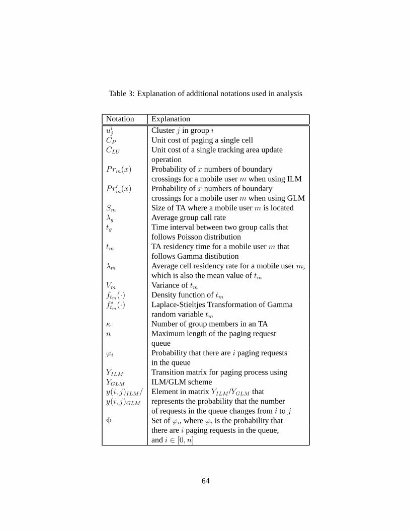
Table 3: Explanation of additional notations used in analysis
Notation Explanation
uij Clusterj in groupi
CP Unit cost of paging a single cellCLU Unit cost of a single tracking area update
operationPrm(x) Probability ofx numbers of boundary
crossings for a mobile userm when using ILMPr′m(x) Probability ofx numbers of boundary
crossings for a mobile userm when using GLMSm Size of TA where a mobile userm is locatedλg Average group call ratetg Time interval between two group calls that
follows Poisson distributiontm TA residency time for a mobile userm that
follows Gamma distibutionλm Average cell residency rate for a mobile userm,
which is also the mean value oftmVm Variance oftmftm(·) Density function oftmf ∗tm(·) Laplace-Stieltjes Transformation of Gamma
random variabletmκ Number of group members in an TAn Maximum length of the paging request
queueϕi Probability that there arei paging requests
in the queueYILM Transition matrix for paging process usingYGLM ILM/GLM schemey(i, j)ILM/ Element in matrixYILM /YGLM thaty(i, j)GLM represents the probability that the number
of requests in the queue changes fromi to jΦ Set ofϕi, whereϕi is the probability that
there arei paging requests in the queue,andi ∈ [0, n]
64

Table 4: Data sets used
Parameters Real Trace [7] SLAW Data [47]
Number of users 39 100Duration 10 hours 24 hours
Interval of data 30 seconds 60 secondsSubgroup every 15 minutes every 30 minutes
Regeneration
Table 5: Impact of threshold on average paging success rate
Real Trace SLAW DataThreshold Best Worst Best Worst
0.3 0.8910 0.8821 0.9166 0.91410.4 0.9038 0.8962 0.9244 0.92310.5 0.8949 0.8840 0.9167 0.91410.7 0.8853 0.8763 0.8654 0.85580.8 0.8821 0.8705 0.8545 0.84290.9 0.8833 0.8712 0.8494 0.8397
65
CHAPTER 5
ENODEB CONTROL WITH SDN AND NVF FOR ENERGY SAVING
Limitations of cellular networks arise from vendor-specific configuration inter-
faces and communications through complex control plane protocols [43]. As shown in
Figure 36, a Radio Resource Control (RRC) such as mobility management, paging con-
trol, and security management are currently included in each eNodeB operation [42].
An emerging network architecture, SDN, simplifies network management and en-
ables researchers to innovate networking and communication by decoupling the control
plane from the data plane. By introducing the concept of SDN into cellular networks,
the control plane of eNodeB moves to a separated controller to enable global control and
efficient management in cellular networks. We suggest decoupling the network function
that focuses on optimizing energy consumption of eNodeB.
In this section, we present our proposed architecture, Siesta, in cellular networks
and cell management algorithms for energy efficient software-defined eNodeB control.
5.1 Siesta Architecture
We note that our proposed architecture is based on LTE or LTE-Advanced. The
eNodeB in LTE and LTE-Advanced is responsible for radio resource allocation, handover,
and paging control. [43] discusses the lack of central control of eNodeBs results in ineffi-
cient radio resource control.
66

Figure 36: eNodeB (LTE, LTE-A) protocol stack with combinedcontrol and data planes
We suggest to virtualize the network function of the eNodeB power control with
placing Siesta above the network controller. The Siesta module handles the eNodeB
power control decisions such as sleep and wake-up modes, andassists user mobility and
handover process. The detailed functionality of the Siestain Figure 37 is as follows:
a) eNodeB power control: The eNodeB power mode is defined by the Siesta through a
cell operation algorithm. For power mode decisions, the history of previous power con-
sumption and network elements information is considered. The energy-aware cell man-
agement algorithm gives a decision on the eNodeB status and user coverage. The detailed
algorithm is presented in Section 5.4.
b) Mobility management: Depending on the eNodeB status decision, some of the users
67
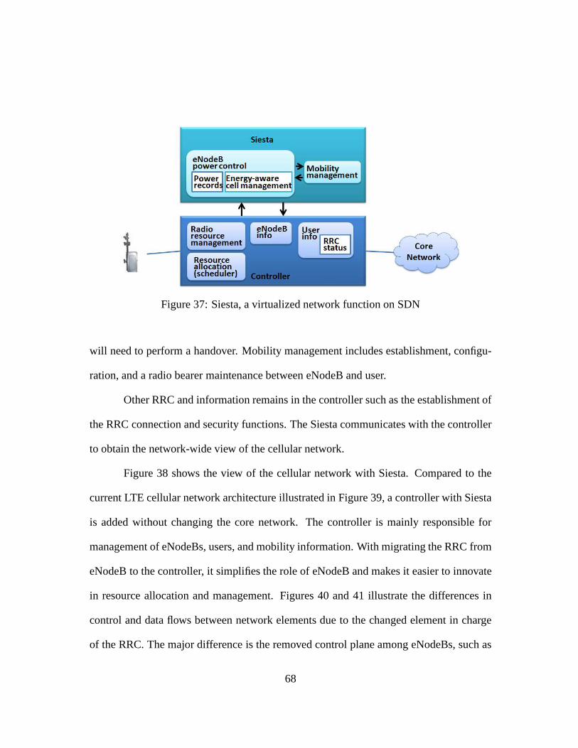
Figure 37: Siesta, a virtualized network function on SDN
will need to perform a handover. Mobility management includes establishment, configu-
ration, and a radio bearer maintenance between eNodeB and user.
Other RRC and information remains in the controller such as the establishment of
the RRC connection and security functions. The Siesta communicates with the controller
to obtain the network-wide view of the cellular network.
Figure 38 shows the view of the cellular network with Siesta.Compared to the
current LTE cellular network architecture illustrated in Figure 39, a controller with Siesta
is added without changing the core network. The controller is mainly responsible for
management of eNodeBs, users, and mobility information. With migrating the RRC from
eNodeB to the controller, it simplifies the role of eNodeB andmakes it easier to innovate
in resource allocation and management. Figures 40 and 41 illustrate the differences in
control and data flows between network elements due to the changed element in charge
of the RRC. The major difference is the removed control planeamong eNodeBs, such as
68

an inter-handover and paging, since the eNodeBs are now mainly responsible for the data
plane. Information handled by Siesta through the controller is as follows:
• Set of eNodeBs with idi: {ei|i = 1, ..., k}
• Traffic load ofei: T icurr,current traffic,T i
min, minimum threshold ofei, T imax, maxi-
mum threshold ofei.
• Users’ spatial information: idi of current serving eNodeB and neighbor eNodeBs
for each user.
• Total energy consumption of a network in durationτ : P (τ)
The necessary global information includes the traffic load and coverage range in-
formation of each eNodeB and spatial information of the users. The information of current
and possible serving eNodeB will be used to identify user coverage for different eNodeB
status. With network-wide information and virtualized control, the network with Siesta
can simplify the management of eNodeBs.
5.2 Energy Control with Siesta
The operation of eNodeB can be divided into several mode: sleep mode, when no
user is served and eNodeB is in sleep; active mode, when the eNodeB serves the users;
increased mode when the eNodeB supports more users for theirneighbor eNodeBs. Let
us denote the power consumption of eNodeBs byPsl, Pac, andPin respectively. We use
the following power consumption model for the different modes of eNodeB. The active
mode power model is simplified from [14]. The power level of eNodeBi is determined
by
69
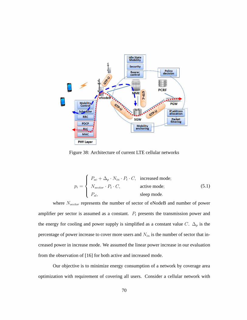
Figure 38: Architecture of current LTE cellular networks
pi =
Pac +∆p ·Nin · Pt · C, increased mode;
Nsector · Pt · C, active mode;
Psl, sleep mode.
(5.1)
whereNsector represents the number of sector of eNodeB and number of power
amplifier per sector is assumed as a constant.Pt presents the transmission power and
the energy for cooling and power supply is simplified as a constant valueC. ∆p is the
percentage of power increase to cover more users andNin is the number of sector that in-
creased power in increase mode. We assumed the linear power increase in our evaluation
from the observation of [16] for both active and increased mode.
Our objective is to minimize energy consumption of a networkby coverage area
optimization with requirement of covering all users. Consider a cellular network with
70
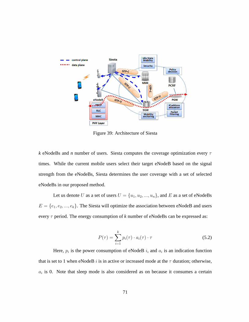
Figure 39: Architecture of Siesta
k eNodeBs andn number of users. Siesta computes the coverage optimizationeveryτ
times. While the current mobile users select their target eNodeB based on the signal
strength from the eNodeBs, Siesta determines the user coverage with a set of selected
eNodeBs in our proposed method.
Let us denoteU as a set of usersU = {u1, u2, ..., un}, andE as a set of eNodeBs
E = {e1, e2, ..., ek}. The Siesta will optimize the association between eNodeB and users
everyτ period. The energy consumption ofk number of eNodeBs can be expressed as:
P (τ) =k
∑
i=1
pi(τ) · ai(τ) · τ (5.2)
Here,pi is the power consumption of eNodeBi, andai is an indication function
that is set to 1 when eNodeBi is in active or increased mode at theτ duration; otherwise,
ai is 0. Note that sleep mode is also considered as on because it consumes a certain
71
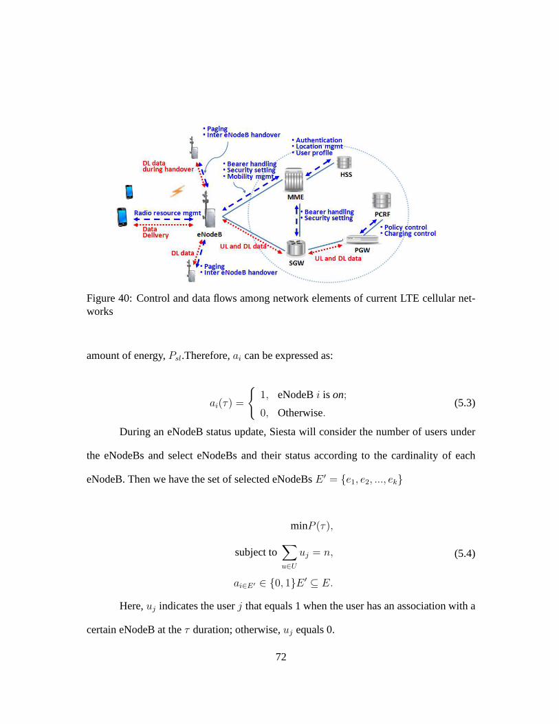
Figure 40: Control and data flows among network elements of current LTE cellular net-works
amount of energy,Psl.Therefore,ai can be expressed as:
ai(τ) =
{
1, eNodeBi is on;
0, Otherwise.(5.3)
During an eNodeB status update, Siesta will consider the number of users under
the eNodeBs and select eNodeBs and their status according tothe cardinality of each
eNodeB. Then we have the set of selected eNodeBsE ′ = {e1, e2, ..., ek}
minP (τ),
subject to∑
u∈U
uj = n,
ai∈E′ ∈ {0, 1}E ′ ⊆ E.
(5.4)
Here,uj indicates the userj that equals 1 when the user has an association with a
certain eNodeB at theτ duration; otherwise,uj equals 0.
72
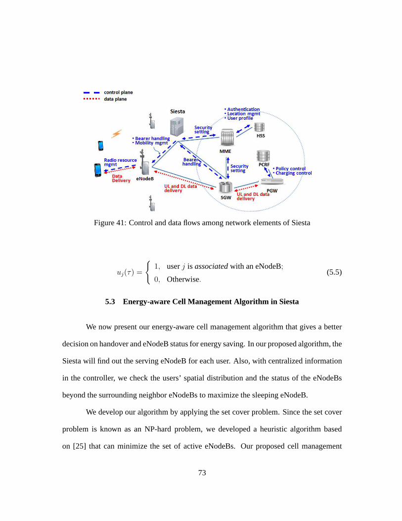
Figure 41: Control and data flows among network elements of Siesta
uj(τ) =
{
1, userj is associatedwith an eNodeB;
0, Otherwise.(5.5)
5.3 Energy-aware Cell Management Algorithm in Siesta
We now present our energy-aware cell management algorithm that gives a better
decision on handover and eNodeB status for energy saving. Inour proposed algorithm, the
Siesta will find out the serving eNodeB for each user. Also, with centralized information
in the controller, we check the users’ spatial distributionand the status of the eNodeBs
beyond the surrounding neighbor eNodeBs to maximize the sleeping eNodeB.
We develop our algorithm by applying the set cover problem. Since the set cover
problem is known as an NP-hard problem, we developed a heuristic algorithm based
on [25] that can minimize the set of active eNodeBs. Our proposed cell management
73
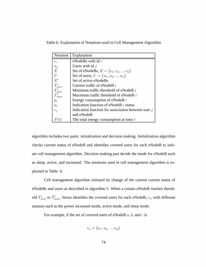
Table 6: Explanation of Notations used in Cell Management Algorithm
Notation Explanation
ei eNodeBs with idiuj Users with idjE Set of eNodeBs,E = {e1, e2, ..., ek}U Set of users,U = {u1, u2, ..., un}E ′ Set of active eNodeBsT icurr Current traffic of eNodeBi
T imin Minimum traffic threshold of eNodeBi
T imax Maximum traffic threshold of eNodeBi
pi Energy consumption of eNodeBiai Indication function of eNodeBi statuscj Indication function for association between userj
and eNodeBP (t) The total energy consumption at timet
algorithm includes two parts: initialization and decisionmaking. Initialization algorithm
checks current status of eNodeB and identifies covered usersfor each eNodeB to initi-
ate cell management algorithm. Decision making part decidethe mode for eNodeB such
as sleep, active, and increased. The notations used in cell management algorithm is ex-
plained in Table 6.
Cell management algorithm initiated by change of the current current status of
eNodeBs and users as described in algorithm 5. When a certaineNodeB reaches thresh-
old T imin or T i
max, Siesta identifies the covered users for each eNodeB,ei, with different
statuses such as the power increased mode, active mode, and sleep mode.
For example, if the set of covered users of eNodeBa, b, andc is
ea = {u1, u2, ..., uq}
74
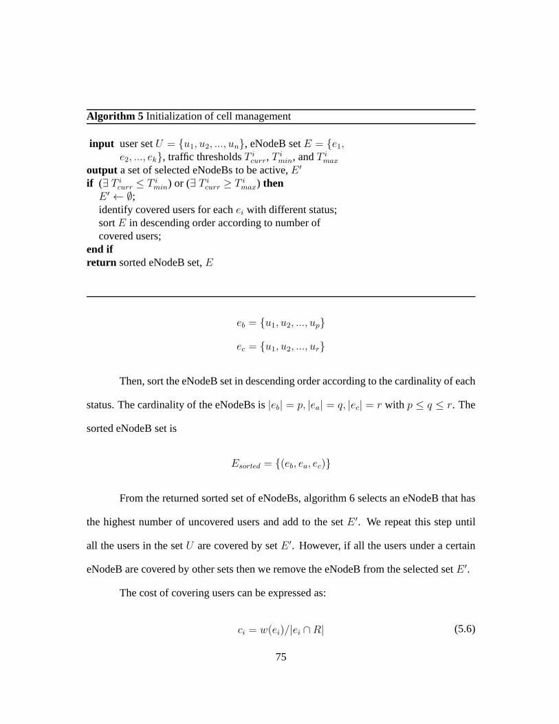
Algorithm 5 Initialization of cell management
input user setU = {u1, u2, ..., un}, eNodeB setE = {e1,e2, ..., ek}, traffic thresholdsT i
curr, Timin, andT i
max
output a set of selected eNodeBs to be active,E ′
if (∃ T icurr ≤ T i
min) or (∃ T icurr ≥ T i
max) thenE ′ ← ∅;identify covered users for eachei with different status;sortE in descending order according to number ofcovered users;
end ifreturn sorted eNodeB set,E
eb = {u1, u2, ..., up}
ec = {u1, u2, ..., ur}
Then, sort the eNodeB set in descending order according to the cardinality of each
status. The cardinality of the eNodeBs is|eb| = p, |ea| = q, |ec| = r with p ≤ q ≤ r. The
sorted eNodeB set is
Esorted = {(eb, ea, ec)}
From the returned sorted set of eNodeBs, algorithm 6 selectsan eNodeB that has
the highest number of uncovered users and add to the setE ′. We repeat this step until
all the users in the setU are covered by setE ′. However, if all the users under a certain
eNodeB are covered by other sets then we remove the eNodeB from the selected setE ′.
The cost of covering users can be expressed as:
ci = w(ei)/|ei ∩ R| (5.6)
75
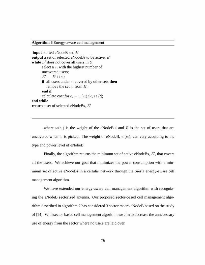
Algorithm 6 Energy-aware cell management
input sorted eNodeB set,Eoutput a set of selected eNodeBs to be active,E ′
while E ′ does not cover all users inUselect aei with the highest number ofuncovered users;E ′ ← E ′ ∪ ei;if all users underei covered by other setsthen
remove the setei fromE ′;end ifcalculate cost forci = w(ei)/|ei ∩ R|;
end whilereturn a set of selected eNodeBs,E ′
wherew(ei) is the weight of the eNodeBi andR is the set of users that are
uncovered whenei is picked. The weight of eNodeB,w(ei), can vary according to the
type and power level of eNobeB.
Finally, the algorithm returns the minimum set of active eNodeBs,E ′, that covers
all the users. We achieve our goal that minimizes the power consumption with a min-
imum set of active eNodeBs in a cellular network through the Siesta energy-aware cell
management algorithm.
We have extended our energy-aware cell management algorithm with recogniz-
ing the eNodeB sectorized antenna. Our proposed sector-based cell management algo-
rithm described in algorithm 7 has considered 3 sector macroeNodeB based on the study
of [14]. With sector-based cell management algorithm we aimto decrease the unnecessary
use of energy from the sector where no users are laid over.
76
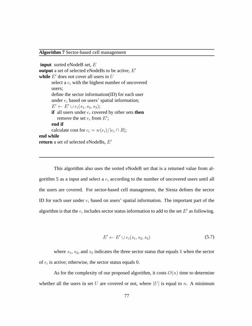
Algorithm 7 Sector-based cell management
input sorted eNodeB set,Eoutput a set of selected eNodeBs to be active,E ′
while E ′ does not cover all users inUselect aei with the highest number of uncoveredusers;define the sector information(ID) for each userunderei based on users’ spatial information;E ′ ← E ′ ∪ ei(s1, s2, s3);if all users underei covered by other setsthen
remove the setei fromE ′;end ifcalculate cost forci = w(ei)/|ei ∩ R|;
end whilereturn a set of selected eNodeBs,E ′
This algorithm also uses the sorted eNodeB set that is a returned value from al-
gorithm 5 as a input and select aei according to the number of uncovered users until all
the users are covered. For sector-based cell management, the Siesta defines the sector
ID for each user underei based on users’ spatial information. The important part of the
algorithm is that theei includes sector status information to add to the setE ′ as following.
E ′ ← E ′ ∪ ei(s1, s2, s3) (5.7)
wheres1, s2, ands3 indicates the three sector status that equals 1 when the sector
of ei is active; otherwise, the sector status equals 0.
As for the complexity of our proposed algorithm, it costsO(n) time to determine
whether all the users in setU are covered or not, where|U | is equal ton. A minimum
77

subsetE ′ can be found inO(log k), where there isk number of eNodeBs in setE. Con-
sequently, the total time complexity of our algorithm isO(n log k).
78

5.4 Siesta Cell Management
(a) SLAKE [60] (b) Cell zooming [59]
(c) Relax [33] (d) Siesta
Figure 42: Existing eNodeB sleep and wake-up schemes for energy saving (solid line:control plane, dotted line: control message exchange for eNodeB sleep)
A global view of cellular networks provides benefits not onlyin power saving but
also in a control procedure. First, we describe the advantage in the control message ex-
change for RAN. Then, the reduced control message for the core network during the han-
dover procedure are compare to the current LTE cellular networks is illustrated. Finally,
we present the energy saving scenario that increases the number of sleeping eNodeBs
with the view beyond the neighbor eNodeBs.
79

0 2 4 6 80
5
10
15
20
25
30
35
Number of neighbor eNodeB
Num
ber
of m
essa
ges
(dur
ing
T on+
Tof
f)
Cell zooming−DCell zooming−CRelaxSiesta
(a)Control message exchange (b)Comparison of message exchange
Figure 43: Control message of Siesta for eNodeB status change
5.4.1 Control Message Comparison
We first explain the control message exchanges of prior eNodeB sleep and wake-
up algorithms. Then we compare the number of message exchange with Siesta during the
transition of eNodeB status.
Description of previous studies: A distributed algorithmSLAKE[60] that communicates
with the only neighbors for eNodeB’s switch on-and-off and zooming is illustrated in
Figure 42(a). In this algorithm, each eNodeB has an RRC procedure so that the decision
for the sleep and wake-up mode is made by eNodeB itself after contact with its neighbor
nodes. Similarly, distributed schemes are proposed in [40,67]. Although these methods
suggest different algorithms, the eNodeB still needs to contact all neighbors for a deci-
sion. A centralized algorithmCell Zooming[59] that introduces a new component and
corresponding functionalities is described in Figure 42(b). For central control there is a
80
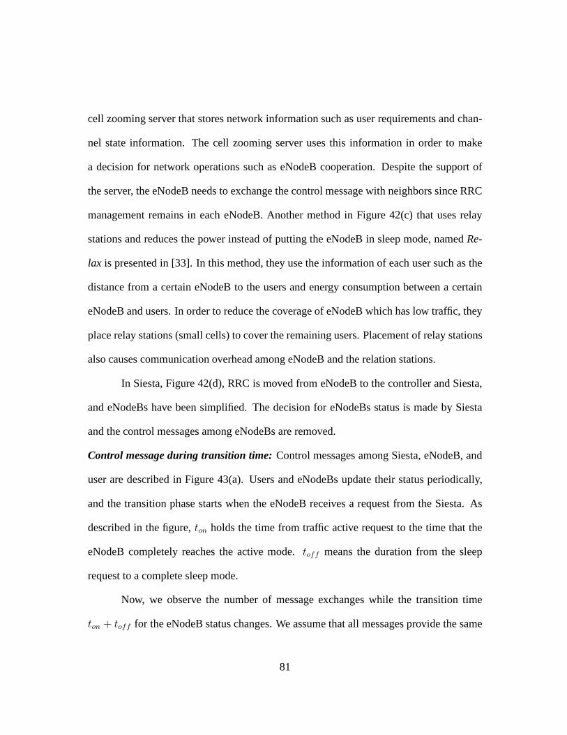
cell zooming server that stores network information such asuser requirements and chan-
nel state information. The cell zooming server uses this information in order to make
a decision for network operations such as eNodeB cooperation. Despite the support of
the server, the eNodeB needs to exchange the control messagewith neighbors since RRC
management remains in each eNodeB. Another method in Figure42(c) that uses relay
stations and reduces the power instead of putting the eNodeBin sleep mode, namedRe-
lax is presented in [33]. In this method, they use the information of each user such as the
distance from a certain eNodeB to the users and energy consumption between a certain
eNodeB and users. In order to reduce the coverage of eNodeB which has low traffic, they
place relay stations (small cells) to cover the remaining users. Placement of relay stations
also causes communication overhead among eNodeB and the relation stations.
In Siesta, Figure 42(d), RRC is moved from eNodeB to the controller and Siesta,
and eNodeBs have been simplified. The decision for eNodeBs status is made by Siesta
and the control messages among eNodeBs are removed.
Control message during transition time: Control messages among Siesta, eNodeB, and
user are described in Figure 43(a). Users and eNodeBs updatetheir status periodically,
and the transition phase starts when the eNodeB receives a request from the Siesta. As
described in the figure,ton holds the time from traffic active request to the time that the
eNodeB completely reaches the active mode.toff means the duration from the sleep
request to a complete sleep mode.
Now, we observe the number of message exchanges while the transition time
ton + toff for the eNodeB status changes. We assume that all messages provide the same
81
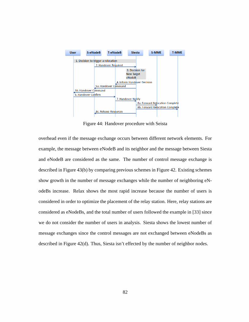
Figure 44: Handover procedure with Seista
overhead even if the message exchange occurs between different network elements. For
example, the message between eNodeB and its neighbor and themessage between Siesta
and eNodeB are considered as the same. The number of control message exchange is
described in Figure 43(b) by comparing previous schemes in Figure 42. Existing schemes
show growth in the number of message exchanges while the number of neighboring eN-
odeBs increase. Relax shows the most rapid increase becausethe number of users is
considered in order to optimize the placement of the relay station. Here, relay stations are
considered as eNodeBs, and the total number of users followed the example in [33] since
we do not consider the number of users in analysis. Siesta shows the lowest number of
message exchanges since the control messages are not exchanged between eNodeBs as
described in Figure 42(d). Thus, Siesta isn’t effected by the number of neighbor nodes.
82

Figure 45: Scenario: Initial step
5.4.2 Handover Procedure with Siesta
The benefit of Siesta is also revealed in the handover procedure. Figure 44 il-
lustrates the handover procedure in Siesta through the controller. Whenever the eNodeB
encounters the threshold, Siesta decides whether the eNodeB changes the status or not.
Suppose the decision is made to change the source-eNodeB (S-eNodeB) status. When
Siesta sends the status change request to S-eNodeB, the users covered by S-eNodeB will
receive the information. Then, the handover procedure starts.
The procedure can be described in three phases:
Phase1: Inform decision to access network S-eNodeB sends the request message for a
handover to Siesta. Siesta determines the new target eNodeBfor each user and informs
the handover decision to the target-eNodeB (T-eNodeB).
Phase2: Handover between S-eNodeB and T-eNodeB The handover command transfer
to the user through the S-eNodeB and the user will response tothe T-eNodeB with a
83

Figure 46: Scenario without centralized view
confirmation message. The T-eNodeB notifies handover to Siesta.
Phase3: Report handover completion to the core network elements Siesta will forward
the relocation complete message to both source MME and target MME while allowing
the resource release from the S-eNodeB.
Compare to the traditional LTE handover procedure [74], thetotal number of mes-
sage exchange is reduced and the message to MME is significantly decreased.
5.4.3 Energy Saving Scenario
The global view of Siesta enables selecting the minimum set of active eNodeBs.
Figure 47 illustrates the scenario that information beyondthe neighbors empowers a re-
duction in the total energy consumption.
Supposee1, e2, e3, ande4 has low traffic with a nighttime traffic decrease. The
e5 also has low traffic ande6 ande7 have high traffic ande6 cannot support more users.
84
Figure 47: Energy saving scenario with Siesta
The e8, e9, ande10 have medium traffic. Note that the users are described asUE in
Figure 46(a), and the users will be supported by the eNodeB which provides higher signal
strength.
Let’s assumee1 reaches a minimum threshold with lowest traffic and the traffic
of e2, e3, ande4 is close to the minimum threshold as described in Figure 46(a). Then
as illustrated in Figure 47(b) Siesta will calculate power consumptionP1 with the ex-
pected cell operation algorithm to reselect eNodeBs.P1 includes the sleep mode energy
consumption ofe1 and the increased mode ofe2, e3, ande7. In terms of handover,UE1
andUE2 are covered bye7, UE3 andUE4 are covered bye2, andUE5 is covered bye3.
However, Siesta considers beyond the neighbors’ status as illustrated in Figure 47. Siesta
knows thate2, e3, ande4 are close to the minimum threshold with low traffic ande8, e9,
ande10 can support the users frome2, e3, ande4, as well. If all of users undere2, e3, and
e4 can be covered by other eNodeBs, Siesta calculates power consumptionP2 for e2, e3,
85

Figure 48: Architecture of LTE-Sim (Current LTE networks)
ande4 sleep. Finally, Siesta compares the power consumptionP1 andP2, then makes the
decision to sleepe2, e3, ande4 sinceP2 is smaller thanP1 as shown in Figure 47(c).
Here, if Siesta does not consider the neighbors’ status ofe1 thene1 will go to sleep
and other neighbors need to stay in active mode with increased traffic to take care of the
users frome1. However, with a global view of the network, some eNodeBs stay in active
mode if they have a possibility to make more eNodeBs sleep. Moreover,e5 gains a greater
possibility for the sleep mode by increasing the power ofe1.
5.5 Evaluations with LTE Simulator
We have conducted evaluations to assess the performance of Siesta cell operation
algorithm using a simulator called LTE-Sim [62] as well as trace-driven simulation. With
LTE-sim, we have compared Siesta with current LTE network. Also, performance of
Siesta is compared with a existing distributed algorithm [60] that is a representative sleep
86
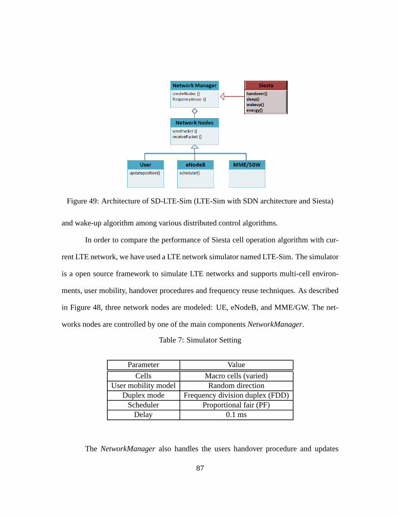
Figure 49: Architecture of SD-LTE-Sim (LTE-Sim with SDN architecture and Siesta)
and wake-up algorithm among various distributed control algorithms.
In order to compare the performance of Siesta cell operationalgorithm with cur-
rent LTE network, we have used a LTE network simulator named LTE-Sim. The simulator
is a open source framework to simulate LTE networks and supports multi-cell environ-
ments, user mobility, handover procedures and frequency reuse techniques. As described
in Figure 48, three network nodes are modeled: UE, eNodeB, and MME/GW. The net-
works nodes are controlled by one of the main componentsNetworkManager.
Table 7: Simulator Setting
Parameter Value
Cells Macro cells (varied)User mobility model Random direction
Duplex mode Frequency division duplex (FDD)Scheduler Proportional fair (PF)
Delay 0.1 ms
The NetworkManageralso handles the users handover procedure and updates
87
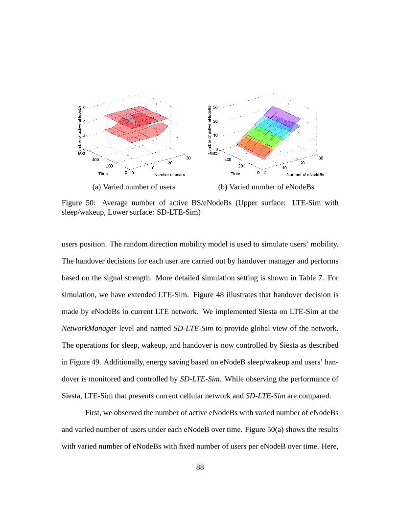
(a) Varied number of users (b) Varied number of eNodeBs
Figure 50: Average number of active BS/eNodeBs (Upper surface: LTE-Sim withsleep/wakeup, Lower surface: SD-LTE-Sim)
users position. The random direction mobility model is usedto simulate users’ mobility.
The handover decisions for each user are carried out by handover manager and performs
based on the signal strength. More detailed simulation setting is shown in Table 7. For
simulation, we have extended LTE-Sim. Figure 48 illustrates that handover decision is
made by eNodeBs in current LTE network. We implemented Siesta on LTE-Sim at the
NetworkManagerlevel and namedSD-LTE-Simto provide global view of the network.
The operations for sleep, wakeup, and handover is now controlled by Siesta as described
in Figure 49. Additionally, energy saving based on eNodeB sleep/wakeup and users’ han-
dover is monitored and controlled bySD-LTE-Sim. While observing the performance of
Siesta, LTE-Sim that presents current cellular network andSD-LTE-Simare compared.
First, we observed the number of active eNodeBs with varied number of eNodeBs
and varied number of users under each eNodeB over time. Figure 50(a) shows the results
with varied number of eNodeBs with fixed number of users per eNodeB over time. Here,
88
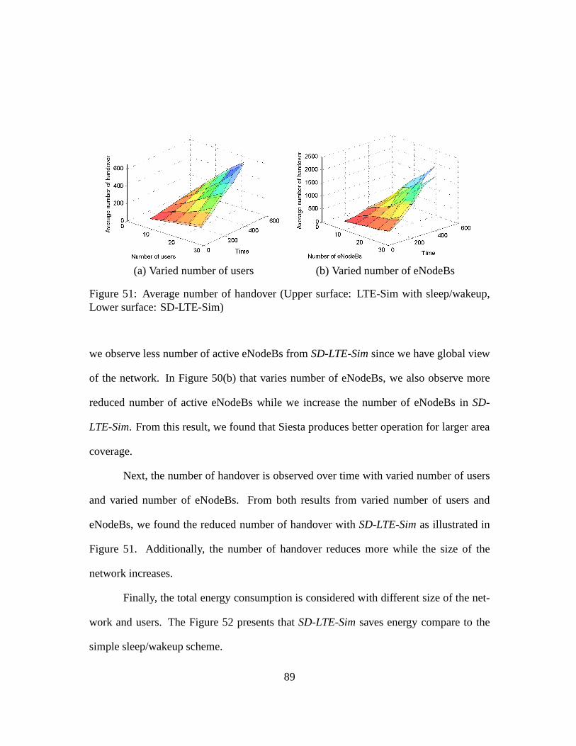
(a) Varied number of users (b) Varied number of eNodeBs
Figure 51: Average number of handover (Upper surface: LTE-Sim with sleep/wakeup,Lower surface: SD-LTE-Sim)
we observe less number of active eNodeBs fromSD-LTE-Simsince we have global view
of the network. In Figure 50(b) that varies number of eNodeBs, we also observe more
reduced number of active eNodeBs while we increase the number of eNodeBs inSD-
LTE-Sim. From this result, we found that Siesta produces better operation for larger area
coverage.
Next, the number of handover is observed over time with varied number of users
and varied number of eNodeBs. From both results from varied number of users and
eNodeBs, we found the reduced number of handover withSD-LTE-Simas illustrated in
Figure 51. Additionally, the number of handover reduces more while the size of the
network increases.
Finally, the total energy consumption is considered with different size of the net-
work and users. The Figure 52 presents thatSD-LTE-Simsaves energy compare to the
simple sleep/wakeup scheme.
89
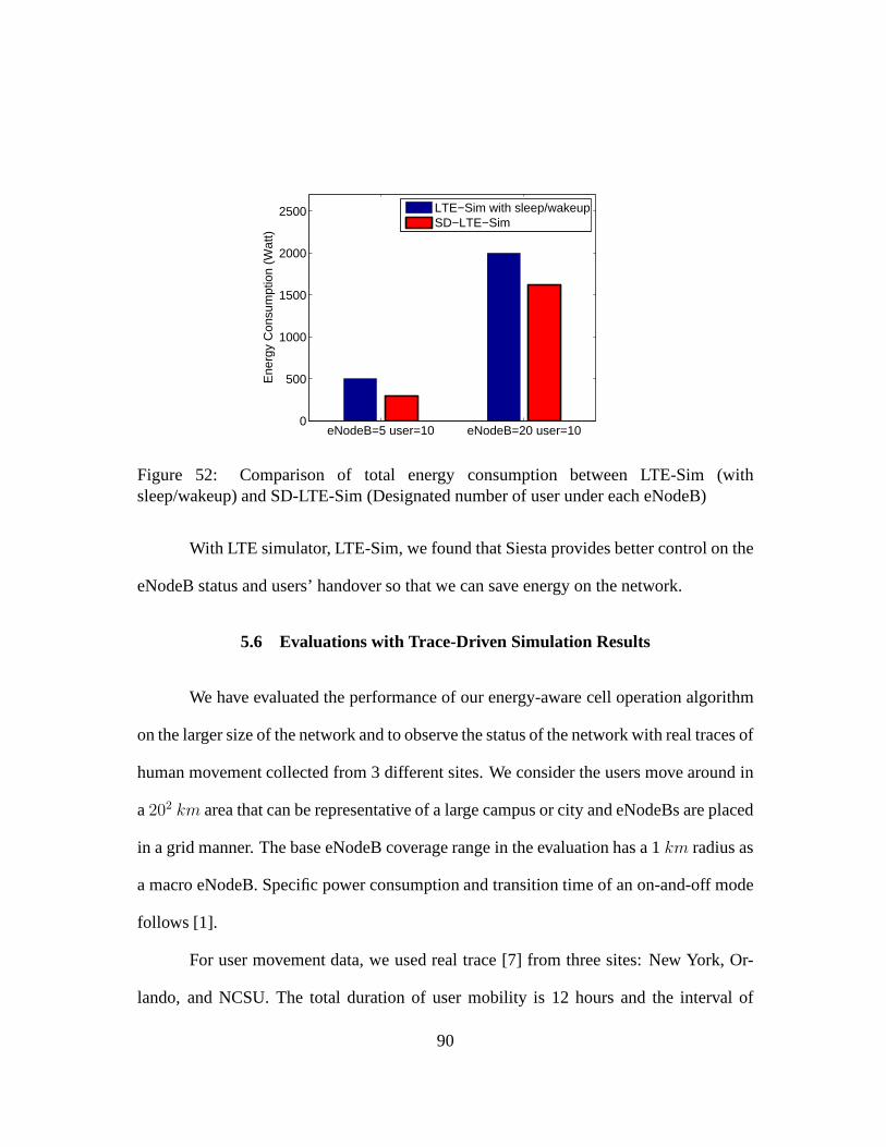
eNodeB=5 user=10 eNodeB=20 user=100
500
1000
1500
2000
2500
Ene
rgy
Con
sum
ptio
n (W
att)
LTE−Sim with sleep/wakeupSD−LTE−Sim
Figure 52: Comparison of total energy consumption between LTE-Sim (withsleep/wakeup) and SD-LTE-Sim (Designated number of user under each eNodeB)
With LTE simulator, LTE-Sim, we found that Siesta provides better control on the
eNodeB status and users’ handover so that we can save energy on the network.
5.6 Evaluations with Trace-Driven Simulation Results
We have evaluated the performance of our energy-aware cell operation algorithm
on the larger size of the network and to observe the status of the network with real traces of
human movement collected from 3 different sites. We consider the users move around in
a202 km area that can be representative of a large campus or city and eNodeBs are placed
in a grid manner. The base eNodeB coverage range in the evaluation has a 1km radius as
a macro eNodeB. Specific power consumption and transition time of an on-and-off mode
follows [1].
For user movement data, we used real trace [7] from three sites: New York, Or-
lando, and NCSU. The total duration of user mobility is 12 hours and the interval of
90
Table 8: Data sets used (Real traces)
Trace Site New York Orlando NCSU
Number of users 39 41 35Total visited cells 72 cells 30 cells 45 cells
location information is 30 seconds. The number of users is 39in New York, 41 in Or-
lando, and 35 in NCSU. The total number of visited cells for each site is 72 cells in New
York, 30 cells in Orlando, and 45 cells in NCSU. Since the number of users of the traces
is relatively small, we assume all cells are initially active with the same level of static
users in each cell. The number of users and the total number ofvisited cells for each site
are described in Table 8. Since the number of users of the traces is relatively small, we
assume all cells are initially active with the same level of static users in each cell. Then,
user mobility is introduced from the human mobility traces creating dynamics of each
cell.
We have conducted evaluations of our energy-aware cell operation algorithm and
have compared its performance with a distributed algorithmthat is a representative sleep
and wake-up algorithm among various distributed control algorithms. In this algorithm,
every active eNodeB makes its own decision independently.
We first observe the effectiveness of Siesta in terms of cell energy saving. We
monitored the eNodeB sleep and awake status over time and compared the difference
between a distributed algorithm and Siesta. Here, we present the results for the New
York trace only due to space limitations. However, other traces exhibit similar patterns.
In Figures 53 and 54, a yellow cell means that its cell range isincreased, a green cell
91

−1 −0.5 0 0.5 1 1.5
x 104
−1
−0.5
0
0.5
1
1.5
2x 10
4
y−co
ordi
nate
x−coordinate
(a) Beginning
−1 −0.5 0 0.5 1 1.5
x 104
−1
−0.5
0
0.5
1
1.5
2x 10
4
y−co
ordi
nate
x−coordinate
(b) After 1 hour
−1 −0.5 0 0.5 1 1.5
x 104
−1
−0.5
0
0.5
1
1.5
2x 10
4
y−co
ordi
nate
x−coordinate
(c) After 2 hours
−1 −0.5 0 0.5 1 1.5
x 104
−1
−0.5
0
0.5
1
1.5
2x 10
4
y−co
ordi
nate
x−coordinate
(d) After 3 hours
Figure 53: eNodeB sleep and awake status over time with a distributed algorithm
indicates that the eNodeB is active, and a blue cell denotes that the eNodeB is in sleep
mode. In the comparison between Figure 53 and Figure 54, it isclearly observed that
Siesta enables more eNodeBs to be in a sleep mode and less to beactive while covering all
the same users. By intelligently increasing a few eNodeBs’ cell coverage, the neighboring
cells find a greater possibility to sleep. The results with sector-based algorithm is shown
in Figure 55
We now directly measure and compare the energy efficiency with respect to the
achieved sleep time, the time spent in state transitions, and the total energy consumption
92

−1 −0.5 0 0.5 1 1.5
x 104
−1
−0.5
0
0.5
1
1.5
2x 10
4
y−co
ordi
nate
x−coordinate
(a) Beginning
−1 −0.5 0 0.5 1 1.5
x 104
−1
−0.5
0
0.5
1
1.5
2x 10
4
y−co
ordi
nate
x−coordinate
(b) After 1 hour
−1 −0.5 0 0.5 1 1.5
x 104
−1
−0.5
0
0.5
1
1.5
2x 10
4
y−co
ordi
nate
x−coordinate
(c) After 2 hours
−1 −0.5 0 0.5 1 1.5
x 104
−1
−0.5
0
0.5
1
1.5
2x 10
4
y−co
ordi
nate
x−coordinate
(d) After 3 hours
Figure 54: eNodeB sleep and awake status over time with Siesta - more sleep eNodeBsare achieved saving energy
of the network. We compared the sleep durations in each hour of data where the sleep
duration for most of the eNodeBs with Siesta is longer than the distributed cell-zooming
algorithm. The longer sleep instances also lead to less eNodeB mode transitions and lower
energy consumption.
Figure 56 shows the cumulative state transition time where the value for each
transition time between modes is set as 17µs following [1], and the transition includes all
changes to reach the new state such as active to sleep or active to increase. The cumulative
transition time exposes the longer sleep instances withoutfrequent status changes that
93
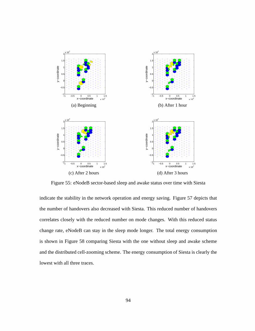
−1 −0.5 0 0.5 1 1.5
x 104
−1
−0.5
0
0.5
1
1.5
2x 10
4
y−co
ordi
nate
x−coordinate
(a) Beginning
−1 −0.5 0 0.5 1 1.5
x 104
−1
−0.5
0
0.5
1
1.5
2x 10
4
y−co
ordi
nate
x−coordinate
(b) After 1 hour
−1 −0.5 0 0.5 1 1.5
x 104
−1
−0.5
0
0.5
1
1.5
2x 10
4
y−co
ordi
nate
x−coordinate
(c) After 2 hours
−1 −0.5 0 0.5 1 1.5
x 104
−1
−0.5
0
0.5
1
1.5
2x 10
4
y−co
ordi
nate
x−coordinate
(d) After 3 hours
Figure 55: eNodeB sector-based sleep and awake status over time with Siesta
indicate the stability in the network operation and energy saving. Figure 57 depicts that
the number of handovers also decreased with Siesta. This reduced number of handovers
correlates closely with the reduced number on mode changes.With this reduced status
change rate, eNodeB can stay in the sleep mode longer. The total energy consumption
is shown in Figure 58 comparing Siesta with the one without sleep and awake scheme
and the distributed cell-zooming scheme. The energy consumption of Siesta is clearly the
lowest with all three traces.
94
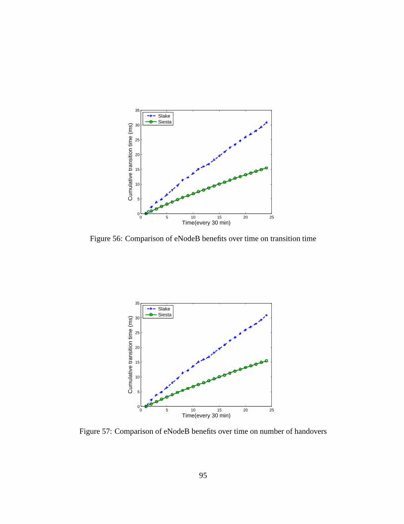
0 5 10 15 20 250
5
10
15
20
25
30
35
Time(every 30 min)
Cum
ulat
ive
tran
sitio
n tim
e (m
s)
SlakeSiesta
Figure 56: Comparison of eNodeB benefits over time on transition time
0 5 10 15 20 250
5
10
15
20
25
30
35
Time(every 30 min)
Cum
ulat
ive
tran
sitio
n tim
e (m
s)
SlakeSiesta
Figure 57: Comparison of eNodeB benefits over time on number of handovers
95
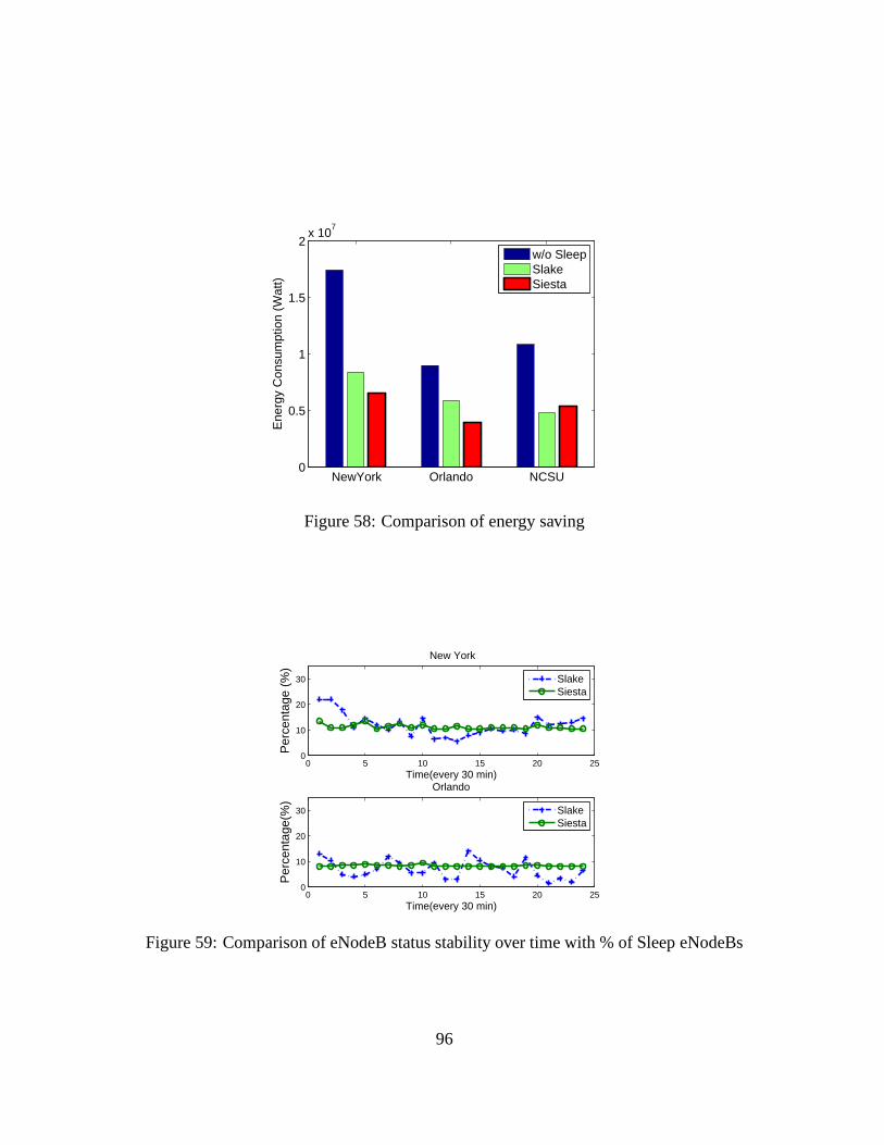
NewYork Orlando NCSU0
0.5
1
1.5
2x 10
7
Ene
rgy
Con
sum
ptio
n (W
att)
w/o SleepSlakeSiesta
Figure 58: Comparison of energy saving
0 5 10 15 20 250
10
20
30
Time(every 30 min)
Per
cent
age
(%)
New York
SlakeSiesta
0 5 10 15 20 250
10
20
30
Time(every 30 min)
Per
cent
age(
%)
Orlando
SlakeSiesta
Figure 59: Comparison of eNodeB status stability over time with % of Sleep eNodeBs
96
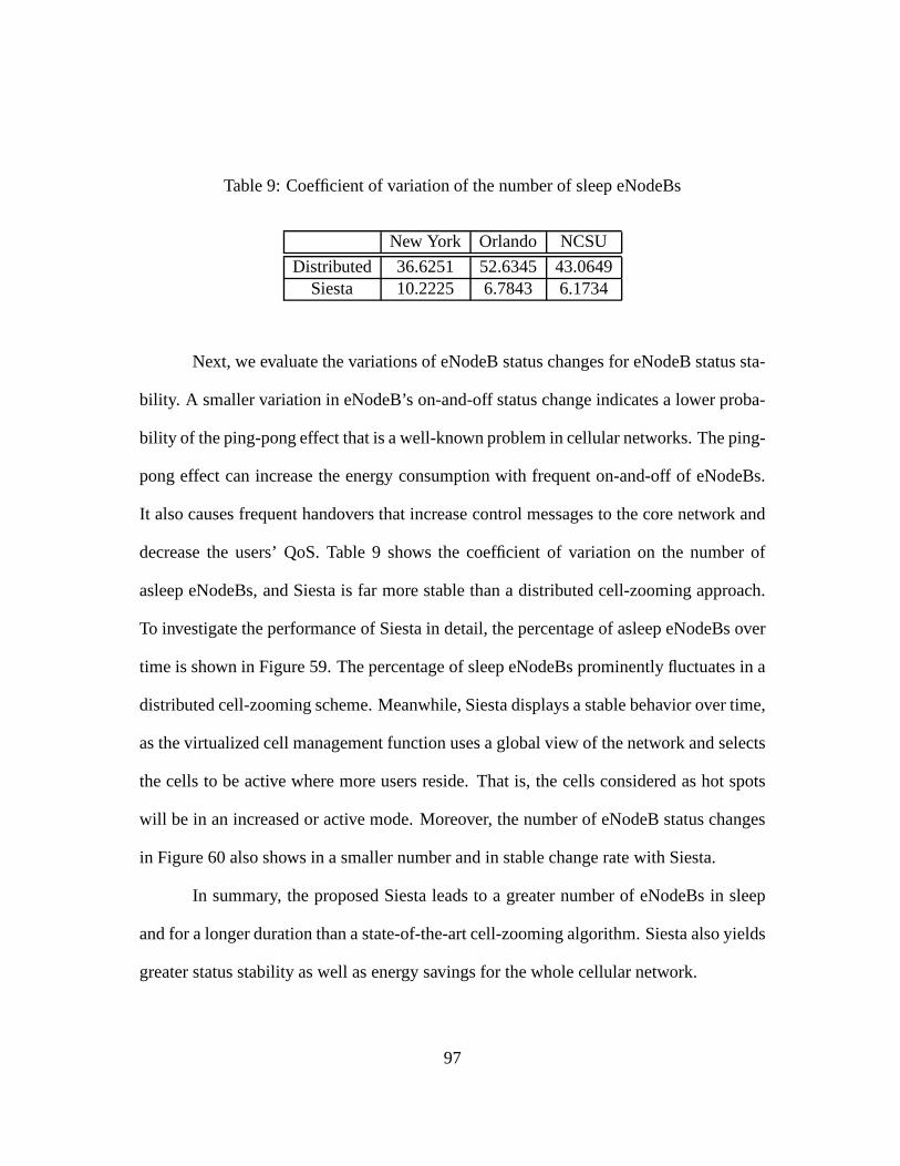
Table 9: Coefficient of variation of the number of sleep eNodeBs
New York Orlando NCSU
Distributed 36.6251 52.6345 43.0649Siesta 10.2225 6.7843 6.1734
Next, we evaluate the variations of eNodeB status changes for eNodeB status sta-
bility. A smaller variation in eNodeB’s on-and-off status change indicates a lower proba-
bility of the ping-pong effect that is a well-known problem in cellular networks. The ping-
pong effect can increase the energy consumption with frequent on-and-off of eNodeBs.
It also causes frequent handovers that increase control messages to the core network and
decrease the users’ QoS. Table 9 shows the coefficient of variation on the number of
asleep eNodeBs, and Siesta is far more stable than a distributed cell-zooming approach.
To investigate the performance of Siesta in detail, the percentage of asleep eNodeBs over
time is shown in Figure 59. The percentage of sleep eNodeBs prominently fluctuates in a
distributed cell-zooming scheme. Meanwhile, Siesta displays a stable behavior over time,
as the virtualized cell management function uses a global view of the network and selects
the cells to be active where more users reside. That is, the cells considered as hot spots
will be in an increased or active mode. Moreover, the number of eNodeB status changes
in Figure 60 also shows in a smaller number and in stable change rate with Siesta.
In summary, the proposed Siesta leads to a greater number of eNodeBs in sleep
and for a longer duration than a state-of-the-art cell-zooming algorithm. Siesta also yields
greater status stability as well as energy savings for the whole cellular network.
97
0 5 10 15 20 250
20
40
60
80
Time(every 30 min)
Num
ber
New York
SlakeSiesta
0 5 10 15 20 250
20
40
60
80
Time(every 30 min)
Num
ber
Orlando
SlakeSiesta
Figure 60: Comparison of eNodeB status stability over time with eNodeB status change
5.7 Summary
We have proposed Siesta (Software-defined energy efficient base station control)
that is a novel NFV of the cell management communicate with SDN controler. Siesta
provides significant benefits over the current cellular networks that suffer from inflexible
management and complex control. Through the eNodeB power control architecture and
the proposed algorithm, Siesta greatly improves energy efficiency in a cellular network
yielding the higher number of eNodeBs in a sleep mode as well as the longer sleep dura-
tions compared with other existing energy efficient techniques. The cell management ar-
chitecture and procedure also greatly simplify the controlover the sleep and awake modes
of eNodeBs and enable an agile handover operations. Siesta exhibits desirable operational
features of stability such as less control message exchanges, less eNodeB status changes,
and less handovers. We have validated the results through both LTE cellular network
simulator that improved with SDN architecture and extensive trace-driven evaluations for
98

observation on the larger network.
99

CHAPTER 6
SUMMARY
The ubiquity of mobile telephony is rapidly expanding, especially with the pop-
ularity of smartphones in recent years. As data traffic and the number of subscribers
increase, there are a number of different challenges and requirements the mobile network
need to e able to handle. Moreover, the expectation on quality and services brings more
challenges to cellular operators and make cellular networks keep evolving. The agility,
flexibility, and manageability of the network can be achieved with SDN and NFV in
cellular networks. This dissertation specifically focusedon functionality of location man-
agement and energy efficiency in cellular systems that can bevirtualized. Furthermore,
SDN gives a centralized view of the network and brings betterresults.
First of all, we proposed a group location management schemeas a virtualized
network function in cellular networks for an improved groupapplication service. The
presence of the virtualized group management function efficiently facilitates the group
location management task and enables a provider to handle a large number of members
and groups that otherwise would be impossible in practice. The group profiling algorithm
dynamically updates its group members’ locations information with clusters of cells or
tracking areas that can be of arbitrary shapes. We validatedthe efficiency of the proposed
scheme with theoretical analyses as well as experiments. The theoretical analyses showed
100
the total signaling traffic cost and significant reduction ofaverage delay. As for the ex-
periments, we used both real traces of human movements and synthetic human mobility
data for the tracking area update and paging costs. Moreover, we investigated the impact
of the parameter that describes the self-similarity of the human walk and suggested the
range of the threshold that decides the size of the TA. To the best of our knowledge, our
work is the first to address the issue of location management for group applications.
For the location management, there are related challenges that need to be ad-
dressed in the future. The benefit of the proposed architecture can be further substantiated
with the development and evaluation of a group call signaling protocol that we plan to ad-
dress in the near future. Also, there is no human group mobility model at the moment, and
it would be useful for evaluations of schemes for group applications. That will also enable
us to perform a detailed theoretical analysis of the proposed group location management
scheme.
Secondly, we have proposed Siesta (Software-defined energyefficient base sta-
tion control) that is a novel network function virtualization (NFV) of the cell manage-
ment. Siesta provides significant benefits over the current cellular networks that suffer
from inflexible management and complex control. Through theeNodeB power control
architecture and the proposed algorithm, Siesta greatly improves energy efficiency in a
cellular network yielding the higher number of eNodeBs in a sleep mode as well as the
longer sleep durations compared with other existing energyefficient techniques. The cell
management architecture and procedure also greatly simplify the control over the sleep
and awake modes of eNodeBs and enable an agile handover operations. Siesta exhibits
101
desirable operational features of stability such as less control message exchanges, less eN-
odeB status changes, and less handovers. We have validated the results through extensive
trace-driven evaluations.
102
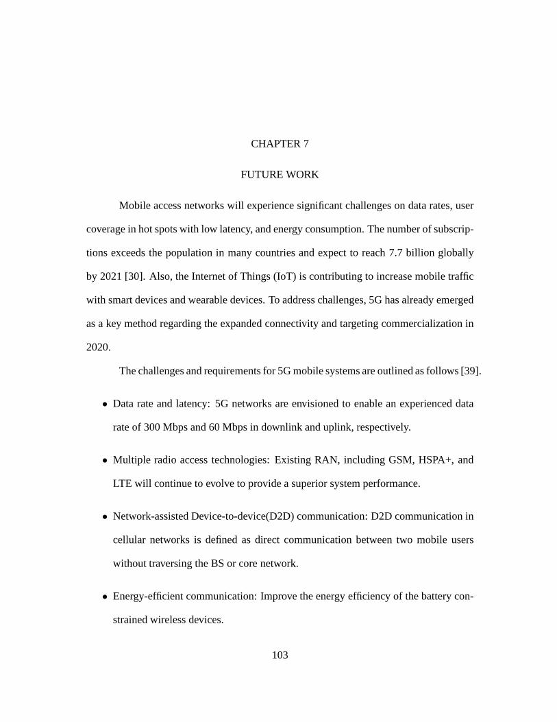
CHAPTER 7
FUTURE WORK
Mobile access networks will experience significant challenges on data rates, user
coverage in hot spots with low latency, and energy consumption. The number of subscrip-
tions exceeds the population in many countries and expect toreach 7.7 billion globally
by 2021 [30]. Also, the Internet of Things (IoT) is contributing to increase mobile traffic
with smart devices and wearable devices. To address challenges, 5G has already emerged
as a key method regarding the expanded connectivity and targeting commercialization in
2020.
The challenges and requirements for 5G mobile systems are outlined as follows [39].
• Data rate and latency: 5G networks are envisioned to enable an experienced data
rate of 300 Mbps and 60 Mbps in downlink and uplink, respectively.
• Multiple radio access technologies: Existing RAN, including GSM, HSPA+, and
LTE will continue to evolve to provide a superior system performance.
• Network-assisted Device-to-device(D2D) communication:D2D communication in
cellular networks is defined as direct communication between two mobile users
without traversing the BS or core network.
• Energy-efficient communication: Improve the energy efficiency of the battery con-
strained wireless devices.
103
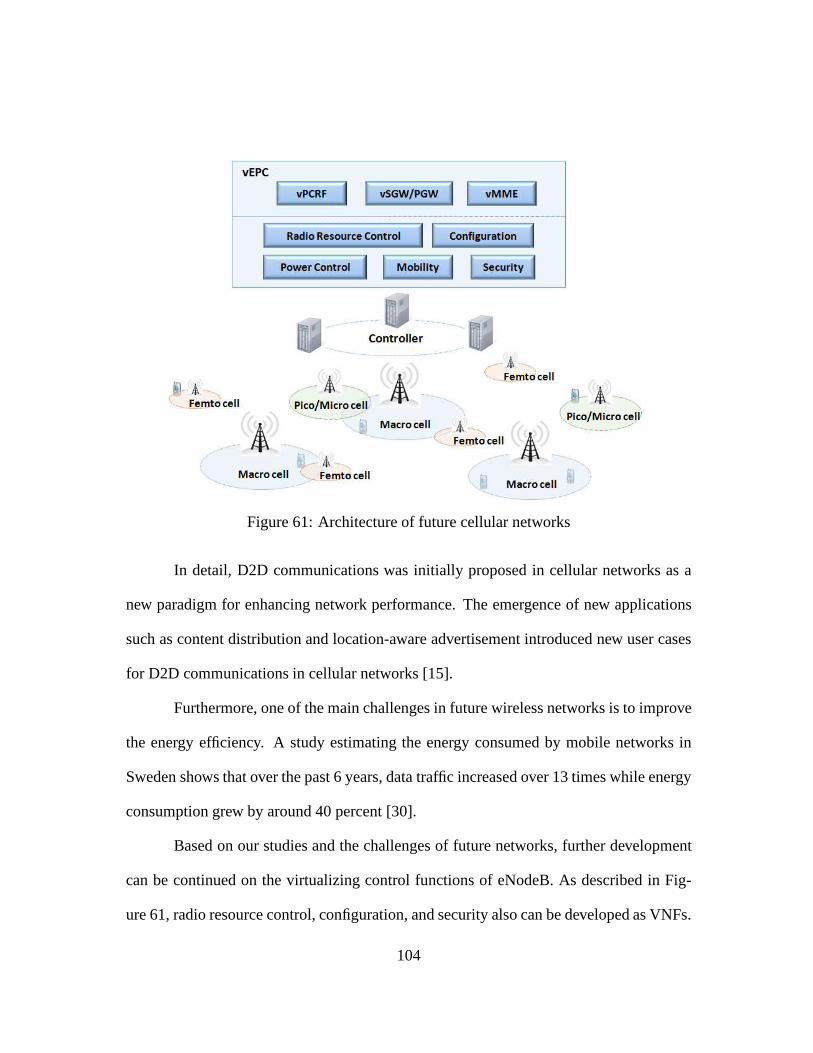
Figure 61: Architecture of future cellular networks
In detail, D2D communications was initially proposed in cellular networks as a
new paradigm for enhancing network performance. The emergence of new applications
such as content distribution and location-aware advertisement introduced new user cases
for D2D communications in cellular networks [15].
Furthermore, one of the main challenges in future wireless networks is to improve
the energy efficiency. A study estimating the energy consumed by mobile networks in
Sweden shows that over the past 6 years, data traffic increased over 13 times while energy
consumption grew by around 40 percent [30].
Based on our studies and the challenges of future networks, further development
can be continued on the virtualizing control functions of eNodeB. As described in Fig-
ure 61, radio resource control, configuration, and securityalso can be developed as VNFs.
104

This can simplify the role of eNodeBs in the network and provide flexibility on manage-
ment. In addition, we also can extend and improve our work with user-centric concept
for heterogeneous deployment on RAN. For example, the eNodeB control can be done
based on users’ needs. Our current work shows that eNodeBs are active and perform
sleep and wakeup based on current traffic. However, eNodeB can be turned on whenever
users’ needs exist with user-centric concept. VNF of power control can handle various
size of eNodeBs such as macro cell, pico/micro cell and femtocell with global view of
the network and offer energy saving and better QoS to users.
105
REFERENCE LIST
[1] Agilent Technologies. http://www.chem.agilent.com.
[2] AT&T Enhanced Push to Talk. http://www.corp.att.com/.
[3] GreenTouch Consortium. http://http://www.greentouch.org.
[4] Nextel Direct Connect . http://www.sprint.com/.
[5] Open Mobile Alliance. http://www.openmobilealliance.org/.
[6] Verizon Wireless – Push to Talk. http://www.verisonwireless.com/.
[7] A Community Resource for Archiving Wireless Data At Dartmouth (CRAWDAD).
http://crawdad.cs.dartmouth.edu/data.php.
[8] Adly, N., and El-Nahas, A. A Profile-Based Hierarchical Location Management
Scheme for Future PCS. InProc. 11th Int. Workshop Database and Expert Systems
Applications (DEXA)(2000), pp. 204 – 208.
[9] Akyildiz, I. F., Gutierrez-Estevez, D. M., and Reyes, E.C. The Evolution to 4G
Cellular Systems: LTE-Advanced.Phys. Commun. 3, 4 (December 2010), 217–244.
[10] Alcatel-Lucent. Introduction to Evolved Packet core.Tech. rep., March 2009.
[11] Alcatel-Lucent. The Journey to Packet Core Virtualization: Evolving the Packet
core to an NFV/SDN Architecture. Tech. rep., 2014.
106
[12] Alcatel-Lucent. The Journey to Packet Core Virtualization: Evolving the Packet
Core to an NFV/SDN Architecture. Tech. rep., February 2014.
[13] Americas, G. The benefits of SON in LTE: Self-optimizingand self-organizing
networks. Tech. rep., December 2009.
[14] Arnold, O., Richter, F., Fettweis, G., and Blume, O. Power Consumption Modeling
of Different Base Station Types in Heterogeneous Cellular Networks. In Future
Network and Mobile Summit(June 2010), pp. 1–8.
[15] Asadi, A., Wang, Q., and Mancuso, V. A Survey on Device-to-Device Communica-
tion in Cellular Networks.Communications Surveys Tutorials, IEEE 16, 4 (2014),
1801–1819.
[16] Auer, G., and et al. D2.3 v2 : Energy efficiency analysis of the reference systems, ar-
eas of improvement and target breakdown. Tech. rep., INFSO-ICT-247733 EARTH
(Energy Aware Radio and NeTwork TecHnologies), 2012.
[17] Bar-Noy, A., Kessler, I., and Sidi, M. Mobile Users: to Update or Not to Update?
In IEEE Proc. 13th Networking for Global Communications (INFOCOM) (1994).
[18] Basta, A., Kellerer, W., Hoffmann, M., Hoffmann, K., and Schmidt, E.-D. A Virtual
SDN-Enabled LTE EPC Architecture: A Case Study for S-/P-Gateways Functions.
In Future Networks and Services (SDN4FNS), IEEE SDN for(2013).
107
[19] Benzaid, C., and Badache, N. A Causal Multicast Protocol for Dynamic Groups
in Cellular Networks. In Proc. Euro American Conf. Telematics and Information
Systems (EATIS)(2008).
[20] Bhaumik, S., Narlikar, G., Chattopadhyay, S., and Kanugovi, S. Breathe to stay
cool: adjusting cell sizes to reduce energy consumption. InProceedings of the
first ACM SIGCOMM workshop on Green networking(2010), Green Networking,
pp. 41–46.
[21] Bousia, A, A. A., Alonso, L., and Verikoukis, C. Green Distance-aware Base Station
Sleeping Algorithm in LTE-Advanced. InCommunications (ICC),IEEE Interna-
tional Conference on(June 2012), pp. 1347–1351.
[22] Cayirci, E., and Akyildiz, I. Optimal Location Area Design to Minimize Registration
Signaling Traffic in Wireless Systems.IEEE Trans. Mobile Computing(2003).
[23] Chen, J.-L., and Wang, K.-C. Reliable WiMAX Multicast Applications. In Proc.
IEEE 8th Int. Conf. Computer and Information Technology Workshops(2008),
pp. 182 – 187.
[24] Chiang, K.-H., and Shenoy, N. Performance of an Overlapped Macro-cell Based
Location Area Scheme. InIEEE Int. Conf. Communications (ICC)(2003).
[25] Chvatal, V. A Greedy Heuristic for the Set-Covering Problem. Mathematics of
Operations Research 4, 3 (1979), 233–235.
108
[26] Claussen, H., Ho, L. T. W., and Pivit, F. Effects of jointmacrocell and residential
picocell deployment on the network energy efficiency. InPersonal, Indoor and
Mobile Radio Communications (PIMRC) IEEE 19th International Symposium on
(September 2008), pp. 1–6.
[27] Committee, O. M. E. Software-defined Networking: The New Norm for Networks,
April 2012.
[28] Communication, F. N. The Benefits of Cloud-RAN Architecture in Mobile Network
Expansion. Tech. rep., 2014.
[29] Elayoubi, S.-E., Saker, L., and Chahed, T. Optimal control for base station sleep
mode in energy efficient radio access networks. InINFOCOM, Proceedings IEEE
(April 2011), pp. 106–110.
[30] Ericsson. Ericsson Mobility Report on the Pulse of the Networked Society. Tech.
rep., November 2015.
[31] Ester, M., Kriegel, H., Sander, J., and Xu, X. A Density-Based Algorithm for Dis-
covering Clusters in Large Spatial Databases with Noise. InProc. 2nd Int. Conf.
Knowledge Discovery and Data mining(1996), pp. 226 – 231.
[32] (ETSI), E. T. S. I. Network Function Virtualization - AnIntroduction, Benefits,
Enablers, Challenges and Call for Action. Tech. rep., October 2012.
109
[33] Gao, C., Zhang, W., Tang, J., Wang, C., Zou, S., and Su, S.Relax, but Do Not Sleep:
A new perspective on Green Wireless Networking. InINFOCOM, Proceedings
IEEE (April 2014), pp. 907–915.
[34] Gomez, K., Rasheed, T., Reynaud, L., and Goratti, L. FME: A Flexible Manage-
ment Entity for virtualizing LTE Evolved Packet Core. InNetwork Operations and
Management Symposium (NOMS),IEEE(2014).
[35] Gudipati, A., Perry, D., Li, L. E., and Katti, S. SoftRAN: Software Defined Radio
Access Network. InProceedings of the Second ACM SIGCOMM Workshop on Hot
Topics in Software Defined Networking (HotSDN)(2013), pp. 25–30.
[36] Haberland, B., Derakhshan, F., Grob-Lipski, H., Klotsche, R., Rehm, W., Schefczik,
P., and Soellner, M. Radio Base Stations in the Cloud.Bell Labs Technical Journal
18, 1 (June 2013), 129–152.
[37] Han, C., Harrold, T., Armour, S., Krikidis, I., Videv, S., Grant, P., Haas, H., Thomp-
son, J., Ku, I., Wang, C.-X., Le, T. A., Nakhai, M., Zhang, J.,and Hanzo, L. Green
radio: radio techniques to enable energy-efficient wireless networks.Communica-
tions Magazine, IEEE 49, 6 (June 2011), 46–54.
[38] Han, I., and Cho, D.-H. Group Location Management for Transportation Systems in
Wireless Cellular Systems. InIEEE 54th Vehicular Technology Conf. (VTC)(2001),
vol. 4, pp. 2726 – 2730.
110
[39] Hossain, E., Rasti, M., Tabassum, H., and Abdelnasser,A. Evolution toward
5G multi-tier cellular wireless networks: An interferencemanagement perspective.
Wireless Communications, IEEE 21, 3 (June 2014), 118–127.
[40] Hossain, M., Munasinghe, K., and Jamalipour, A. A protocooperation-based sleep-
wake architecture for next generation green cellular access networks. In Signal
Processing and Communication Systems (ICSPCS), 4th International Conference
on (December 2010), pp. 1–8.
[41] I, C.-L., Huang, J., Duan, R., Cui, C., Jiang, J., and Li,L. Recent Progress on
C-RAN Centralization and Cloudification.Access, IEEE 2(2014), 1030–1039.
[42] Inc., T. I. LTE in a Nutshell: Protocol Architectur. Tech. rep., 2010.
[43] Jin, X., Li, L. E., Vanbever, L., and Rexford, J. SoftCell: Scalable and Flexible Cel-
lular Core Network Architecture. InProceedings of the Ninth ACM Conference on
Emerging Networking Experiments and Technologies (CoNEXT) (2013), pp. 163–
174.
[44] Kelif, J. M., Coupechoux, M., and Marache, F. Limiting Power Transmission of
Green Cellular Networks: Impact on Coverage and Capacity. In ICC (2010), pp. 1–
6.
[45] Lam, G. H. K., Leong, H. V., and Chan, S. C. F. Reducing Group Management
Overhead in Group-Based Location Management. InProc. 15th Int. Workshop
Database and Expert Systems Applications(2004), pp. 640 – 644.
111

[46] Lee, D. C., jin Kim, H., Lee, J., and Lin, Y. B. Performance Analysis of the Dis-
tributed Location Management Scheme in Large Mobile Networks. Journal of In-
formation Processing Systems 1, 1 (2005), 55 – 61.
[47] Lee, K., Hong, S., Kim, S. J., Rhee, I., and Chong, S. SLAW: A New Mobility
Model for Human Walks. InProc IEEE INFOCOM(2009), pp. 855 – 863.
[48] Li Erran Li, Z. M. M., and Rexford, J. Toward software-defined cellular networks.
In Proc. European Workshop on Software Defined Networking (EWSDN) (October
2012).
[49] Lin, Y. Reducing Location Update Cost in a PCS Network.IEEE/ACM Trans.
Networking 5, 1 (1997), 25 – 33.
[50] Liou, R.-H., Lin, Y.-B., and Tsai, S.-C. An Investigation on LTE Mobility Manage-
ment. Mobile Computing, IEEE Transactions on(2013).
[51] Liu, J., Sacchetti, D., Sailhan, F., and Issarny, V. Group Management for Mobile Ad
Hoc Networks: Design, Implementation and Experiment. InProc. 6th Int. Conf.
Mobile Data Management (MDM)(2005).
[52] Liyanage, M., Gurdrei, A., and Yilanttila, M.Software Defined Mobile Networks -
beyond LTE Network Architecture. No. ISBN 978-1-118-90028-4. Wiley, 2015.
[53] Marsan, M. A., Chiaraviglio, L., Ciullo, D., and Meo, M.OptimalEnergy Savings in
Cellular Access Networks. InIEEE International Conference on Communications
Workshops(June 2009).
112
[54] Marsan, M. A., and Meo, M. Energy Efficient Wireless Internet Access with Coop-
erative Cellular Networks. InComputer Networks(2010).
[55] Mobile, C. C-RAN The Road Towards Green RAN. Tech. rep.,October 2011.
[56] Morosi, S., Del Re, E., and Piunti, P. Traffic based energy saving strategies for green
cellular networks. InEuropean Wireless, 18th European Wireless Conference(April
2012), pp. 1–6.
[57] Networks, F. Network Functions Virtualization - Everything Old Is New Again.
Tech. rep., 2013.
[58] Ng, C. K., and Chan, H. W. Enhanced Distance-Based Location Management of
Mobile Communication Systems Using a Cell Coordinates Approach. IEEE Trans.
Mobile Computing 4, 1.
[59] Niu, Z., Wu, Y., Gong, J., and Yang, Z. Cell zooming for cost-efficient green cellular
networks.Communications Magazine, IEEE 48, 11 (November 2010), 74–79.
[60] Oh, E., Son, K., and Krishnamachari, B. Dynamic Base Station Switching-On/Off
Strategies for Green Cellular Networks.Wireless Communications, IEEE Transac-
tions on 12, 5 (May 2013), 2126–2136.
[61] Parija, S., Nanda, S., Sahu, P., and Singh, S. Novel Intelligent Soft Computing
Techniques for Location Prediction in Mobility Management. In Engineering and
Systems (SCES), Students Conference on(2013).
113
[62] Piro, G., Grieco, L., Boggia, G., Capozzi, F., and Camarda, P. Simulating LTE Cel-
lular Systems: An Open-Source Framework.Vehicular Technology, IEEE Transac-
tions on 60, 2 (February 2011), 498–513.
[63] Pollini, G., and I, C.-L. A Profile-Based Location Strategy and its Performance.
IEEE Journal on Selected Areas in Communications(1997).
[64] Ratnam, K., Matta, I., and Rangarajan, S. A Fully Distributed Location Management
Scheme for Large PCS Networks, 1999.
[65] Roy, A., Misra, A., and Das, S. K. Location Update versusPaging Trade-Off in Cel-
lular Networks: An Approach Based on Vector Quantization.IEEE Trans. Mobile
Computing 6, 12.
[66] Said, S. B. H., Guillouard, K., and Bonnin, J. On the benefit of context-awareness
for security mechanisms in LTE/EPS networks. In24th IEEE Annual Interna-
tional Symposium on Personal, Indoor, and Mobile Radio Communications, PIMRC,
September, 2013(2013).
[67] Saker, L., Elayoubi, S.-E., and Chahed, T. Minimizing Energy Consumption via
Sleep Mode in Green Base Station. InWireless Communications and Networking
Conference (WCNC), IEEE(April 2010), pp. 1–6.
[68] Schmelz, L. C., Berg, J. V. D., Litjens, R., ICT, T., Zetterberg, K., and Amirijoo, M.
Self-organisation in Wireless Networks Use Cases and theirInterrelation. In 22nd
Wireless World Research Forum (WWRF)(May 2009).
114

[69] SDN, and Congress, O. W. Network Functions Virtualisation (NFV) - An Introduc-
tion, Benefits, Enablers, Challenges and Call for Action. Tech. rep.
[70] Simone Morosi, P. P., and Re, E. D. Sleep Mode Managementin Cellular Networks:
A Traffic Based Technique Enabling Energy Saving.Transactions on Emerging
Telecommunications Technologies 24, 3 (2013), 331–341.
[71] Singh, J., and Karnan, M. Using a Novel Intelligent Location Management Strategy
in Cellular Networks. In Signal Acquisition and Processing ICSAP ’10. Interna-
tional Conference on(2010).
[72] Son, K., and Krishnamachari, B. SpeedBalance: Speed-scaling-aware optimal load
balancing for green cellular networks. InINFOCOM, Proceedings IEEE(March
2012), pp. 2816–2820.
[73] Son, K., Oh, E., and Krishnamachari, B. Energy-aware hierarchical cell configu-
ration: From deployment to operation. InComputer Communications Workshops
(INFOCOM WKSHPS),IEEE Conference on(April 2011), pp. 289–294.
[74] Stefania Sesia, Issam Toufik, M. B.LTE - The UMTS Long Term Evolution: From
Theory to Practice. No. ISBN 978-0-470-74288-4. Wiley, 2009.
[75] Tcha, D.-W., Choi, T.-J., and Myung, Y.-S. Location-Area Partitioning in a Cellular
Radio Network. The Journal of the Operational Research Society 48, 11 (1997),
1076 – 1081.
115
[76] Varsamopoulos, G., and Gupta, S. Dynamically AdaptingRegistration Areas to User
Mobility and Call Patterns for Efficient Location Management in PCS Networks.
IEEE/ACM Trans. Networking(2004).
[77] Varsamopoulos, G., and Gupta, S. Optimal Offline and Online Registration Tech-
niques for Location Management with Overlapping Registration Areas.IEEE Trans.
Mobile Computing(2005).
[78] Verkama, M. A Simple Implementation of Distance-BasedLocation Updates. In
IEEE 6th Int. Conf. Universal Personal Communications Record (1997).
[79] Wu, X., Mukherjee, B., and Bhargava, B. A Low-Cost, Low-Delay Location Up-
date/Paging Scheme in Hierarchical Cellular Networks. InProceedings of the 3rd
ACM International Workshop on Data Engineering for Wireless and Mobile Access
(2003), pp. 46 – 50.
[80] Wu, X., Mukherjee, B., and Bhargava, B. A Crossing-TierLocation Update/Paging
Scheme in Hierarchical Cellular Networks.IEEE Trans. Wireless Communications
(2006).
[81] Wuthnow, M., Stafford, M., and Shih, J.IMS: A New Model for Blending Applica-
tions. No. ISBN 1-4200-9285-5. Taylor and Francis, 2009.
VITA
Sunae Shin was born in Seoul, South Korea, on October 11, 1981. Ms. Shin
entered the Kyung Hee University in South Korea in March 2001and graduated in July
2005 with a Bachelor of Engineering degree in Computer Engineering. After graduation,
Ms. Shin came to the USA to study and gained a Master of Sciencedegree in Computer
Science from South Dakota State University at Brookings in South Dakota in December
2007. Her thesis topic was an enhanced retrieval tool for EJBcomponents for components
based software development.
After her Master degree, Ms. Shin joined interdisciplinaryPh.D. curriculum at
the University of Missouri-Kansas City in 2008. Her coordinating discipline is Telecom-
munications and Computer Networking and her co-disciplineis Electrical and Computer
Engineering. Her main research interest and dissertation topic is base station control and
mobility management with software-defined networking for green cellular networks. Ms.
Shin also performed several distinct projects in various areas such as data transfer protocol
using network testbeds, energy efficiency in wireless sensor networks, and smartphone-
based collision avoidance system. Along with research, shehave acquired teaching expe-
riences. She taught Discrete mathematics I and Problem solving & programming lab at
University of Missouri - Kansas City.
During her Ph.D. study, Ms. Shin received the first poster award from the Grace
Hopper Celebration (GHC) regional conference - Missouri, Iowa, Nebraska, and Kansas
Women in Computing (MINKWIC) conference in 2011. She also awarded scholarship of
117
Graduate Assistance Fund (GAF) through UMKC women′s council in 2013 and several
travel grants from GENI Engineering Conference (GEC) in 2013 and Central Area Net-
working and Security workshop (CANSec) in 2014. Additionally, she received Outstand-
ing Ph.D. student award from Telecommunication and Computer Networking discipline
in 2014. She also gained research grant from University of Missouri - Kansas City, School
of Graduate Studies Research award program in 2015.
118