software performance estimation in mpsoc design

HAL Id: tel-00195230https://tel.archives-ouvertes.fr/tel-00195230

Submitted on 10 Dec 2007

HAL is a multi-disciplinary open accessarchive for the deposit and dissemination of sci-entific research documents, whether they are pub-lished or not. The documents may come fromteaching and research institutions in France orabroad, or from public or private research centers.

L’archive ouverte pluridisciplinaire HAL, estdestinée au dépôt et à la diffusion de documentsscientifiques de niveau recherche, publiés ou non,émanant des établissements d’enseignement et derecherche français ou étrangers, des laboratoirespublics ou privés.

Software performance estimation in MPSoC designMarcio Oyamada

To cite this version:Marcio Oyamada. Software performance estimation in MPSoC design. Micro and nanotechnolo-gies/Microelectronics. Institut National Polytechnique de Grenoble - INPG, 2007. English. <tel-00195230>

https://tel.archives-ouvertes.fr/tel-00195230

https://hal.archives-ouvertes.fr

INSTITUT NATIONAL POLYTECHNIQUE DE GRENOBLE N° attribué par la bibliothèque |__|__|__|__|__|__|__|__|__|__|

T H E S E E N C O T U T E L L E I N T E R N A T I O N A L E

pour obtenir le grade de

DOCTEUR DE L’INP Grenoble et

da Universidade Federal do Rio Grande do Sul

Spécialité : Micro Électronique

préparée au laboratoire TIMA

dans le cadre de l’Ecole Doctorale « d’Electronique, Automatique et Traitement du

Signal »

et au laboratoire LSE

dans le cadre du «Programa de Pós-Graduação em Computação »

présentée et soutenue publiquement

par

Marcio Seiji OYAMADA

le 05 décembre 2007

Estimation de performance du logiciel en systèmes multiprocesseur monopuces

Directeur de thèse : Ahmed Amine JERRAYA Directeur de thèse : Flavio Rech WAGNER

JURY

Mme. Florence MARANINCHI , Président M. Luigi CARRO , Rapporteur M. Guido Costa Souza de ARAUJO , Rapporteur M. Ian O’CONNOR , Rapporteur M. Ahmed Amine JERRAYA , Directeur de thèse M. Flavio Rech WAGNER , Directeur de thèse

3

For my family

5

ACKNOWLEDGMENTS

I would like to thank, first and foremost, my advisors Mr. Flavio RECH WAGNER from Universidade Federal do Rio Grande do Sul and Mr. Ahmed Amine JERRAYA from TIMA Laboratory, for their support and encouraging discussions during the thesis development.

I would also like to thank Dr. Florence MARANINCHI, Dr. Ian O’CONNOR and Dr Guido ARAUJO for agreeing to be on my thesis committee and for their comments. Special thanks go to Dr. Luigi CARRO for his encouraging discussions and inspiring ideas.

I would like to acknowledge the students and other staff members in the TIMA laboratory, especially the SLS members: Aimen, Wassin, Iuliana, YoungChul, Lobna, Sang Il, Katalin, Marius, Sonya, Amin, Benaoumeur, Xi and Hao. Special thanks to my “RU copains”: Ivan, Arif, Arnaud and Patrice. I would like to thank Wander, Adriano, Joao and Lazzari for their support in France.

Gostaria de agradecer aos professores, funcionários e alunos do Instituto de Informática. Especialmente para os meus amigos nas horas alegres e também difíceis: Julius, Caco, Fernando, Emerson, Gervini, Leomar, Felipe, Edgard, Mateus, Dalton, Lisane, e os paranaenses Wronski, Jeysson, Luiz e Moratelli.

Agradeço pelo apoio incondicional dos meus pais Hiroshi e Tomie, irmãs Suely e Lucia e irmão Marcelo, além dos meus sobrinhos (trio de diabinhos): Bruno, Thais e Erick. Agradeço também a minha esposa Giovanna, companheira em todos os momentos.

I acknowledge the work of UNIOESTE for the financial support and CAPES for the scholarship during my work in France.

7

TABLE DES MATIÈRES

1 ESTIMATION DE PERFORMANCE EN SYSTEMES MULTIPROCESSEURS MONOPUCES ............................................................ 8

1.1 L’intégration de l’estimation de performance dans le flot ROSES ............. 10 1.2 Estimation de performance basée sur des réseaux neuronaux..................... 11 1.3 L’analyse intégrée de performance des systèmes MPSoC............................ 14

2 ÉTUDE DE CAS DE L’ENCODEUR MPEG4 ........................................... 16

2.1 Flot d’estimation et analyse de performance ................................................. 17 2.2 Estimation au niveau de la spécification......................................................... 18 2.3 Analyse de performance avec un prototype virtuel....................................... 20

3 CONCLUSIONS........................................................................................ 27

3.1 Limitations des méthodes proposées et les perspectives ............................... 28

8

1 ESTIMATION DE PERFORMANCE EN SYSTEMES MULTIPROCESSEURS MONOPUCES

L’augmentation de la capacité d’intégration de transistors permet l’intégration des

processeurs, composants matériel, mémoires, interface digitale e analogique sur une

puce. Actuellement, on constate de plus en plus l’utilisation de plusieurs processeurs

dans une seule puce, appelé MPSoC (multiprocessor system-on-chip). En comparaison

avec des implémentations purement matérielles les processeurs donnent la flexibilité et

hétérogénéité nécessaires dans les systèmes embarqués.

La conception d’un système embarqué est imposée à des contraintes strictes. Le flot

de conception d’un MPSoC demande des outils pour vérifier si les conditions sont

suffisantes. La performance est normalement la principale contrainte pour guider

l’exploitation de l’espace des solutions. Néanmoins, les autres aspects doivent être

évalués dans les étapes initiales du projet, par exemple la puissance et l’énergie.

L’exploration d’un énorme espace d’alternatives est appuyée par des outils

d’estimation.

L’estimation de performance est un processus continu et peut être utilisée aux

différents niveaux d’abstraction comme montre la Figure 1.1. Pendant la spécification

du système, l’estimation de performance aide dans le partitionnement du système en

composants matériels et logiciels, la sélection du processeur, et le mapping des tâches

sur les processeurs.

L’architecture virtuelle est un modèle où le logiciel n’est pas compilé pour le

processeur cible et la communication est faite par des canaux au niveau transactionnel.

Comme l’interconnexion n’est pas encore définie, à ce niveau on exploite les différentes

possibilités d’implémentation des canaux TLM (transaction level model) et de la

structure de communication.

9

Au niveau du bus fonctionnel (bus functional model – BFM) les interfaces

matérielles et logicielles sont déjà raffinés et le logiciel est compilé pour le processeur

cible. A ce niveau, une analyse détaillée de la performance du matériel et du logiciel

sont possibles.

Architecture Virtuelle

Niveau bus fonctionnel

Intégration SoC

Niveau RTL

Outils d’estimation de performance

Raffinage des interfaces logiciel/matériel

Spécification du système

Exploration de l’architecture

Sélection du processeur

Partitionnement des interfaces logiciel/matériel

Mapping de la memóire

Estimation de retards

Domaine de ce travail

Figure 1.1- Estimation de performance et les niveaux d’abstraction dans la conception

d’un MPSoC

En raison de l’augmentation de la partie logicielle et du nombre des processeurs

dans les systèmes embarqués, des outils pour l’estimation de performance sont

nécessaires. Les outils d’estimation de performance sont divisées en deux groupes:

basées sur la simulation et modèles abstraits (MEYEROWITZ, 2004). Les méthodes

basées sur la simulation utilisent un simulateur précis au niveau du cycle pour estimer le

temps d’exécution. De l’autre coté, des modèles abstraits ou analytiques utilisent des

fonctions de coût pour calculer le temps d’exécution du logiciel. Les méthodes au

niveau intermédiaire sont basées sur l’annotation du code avec les coûts d’exécution.

Comme l’application exécute sur le poste de travail, la simulation est plus rapide.

Cette thèse propose des méthodes pour l’estimation de performance, qui sont

nécessaires en raison du grand espace de solutions qui ne peut pas être exploré

manuellement ou vérifié juste quand un prototype matériel est disponible. Un modèle

10

analytique est proposé pour estimer la performance basé sur des réseaux neuronaux au

niveau de la spécification. Des outils ont été développés pour l’analyse de performance

au niveau du bus fonctionnel, en utilisant les prototypes virtuels pour valider d’une

manière intégrée les composants matériels et logiciels. Le prototype virtuel est un

modèle de simulation qui permet une analyse de performance intégrée des composants

matériels et logiciels.

1.1 L’intégration de l’estimation de performance dans le flot ROSES

Cette thèse propose une méthodologie pour l’analyse et l’estimation de performance

dans les systèmes multiprocesseurs monopuces (MPSoC). Le flot de conception ROSES

développé au sein du groupe SLS est utilisé pour guider le flot d’estimation de

performance. L’environnement ROSES permet la génération automatique des interfaces

logicielles et matérielles dans un système MPSoC. Le flot de conception ROSES utilise

comme point de départ pour la génération des interfaces une architecture virtuelle

composée par des composants fonctionnels reliés par de canaux de communication au

niveau transactionnel. Dans l’architecture virtuelle, les composants fonctionnels

décrivent les composants matériels et logiciels du système. Les composants logiciels

sont composés par des tâches, qui communiquent par des canaux logiques.

Dans la cadre de cette thèse, des réseaux neuronaux sont utilisés pour guider la

sélection du processeur pour chaque composant logiciel. Les réseaux neuronaux

apportent une solution efficace pour modéliser le comportement non-linéaire du logiciel

exécutant dans les processeurs avec des caractéristiques comme le pipeline, mémoires

cache et prédiction de branchement. Dans les expériences, on a utilisé différents

processeurs, comme le PowerPC750, l’ADSP, l’ARM946 et un processeur Java.

Après la sélection du processeur, l’environnement ROSES est utilisé pour raffiner

les interfaces matérielles et logicielles et générer un modèle au niveau du bus

fonctionnel (bus functional model - BFM). Dans ce travail, on propose l’utilisation de

prototypes virtuels pour créer des modèles globaux de simulation. La génération

automatique du prototype virtuel à partir d’un modèle de bus fonctionnel généré par

ROSES permet l’analyse de performance et la validation du système.

11

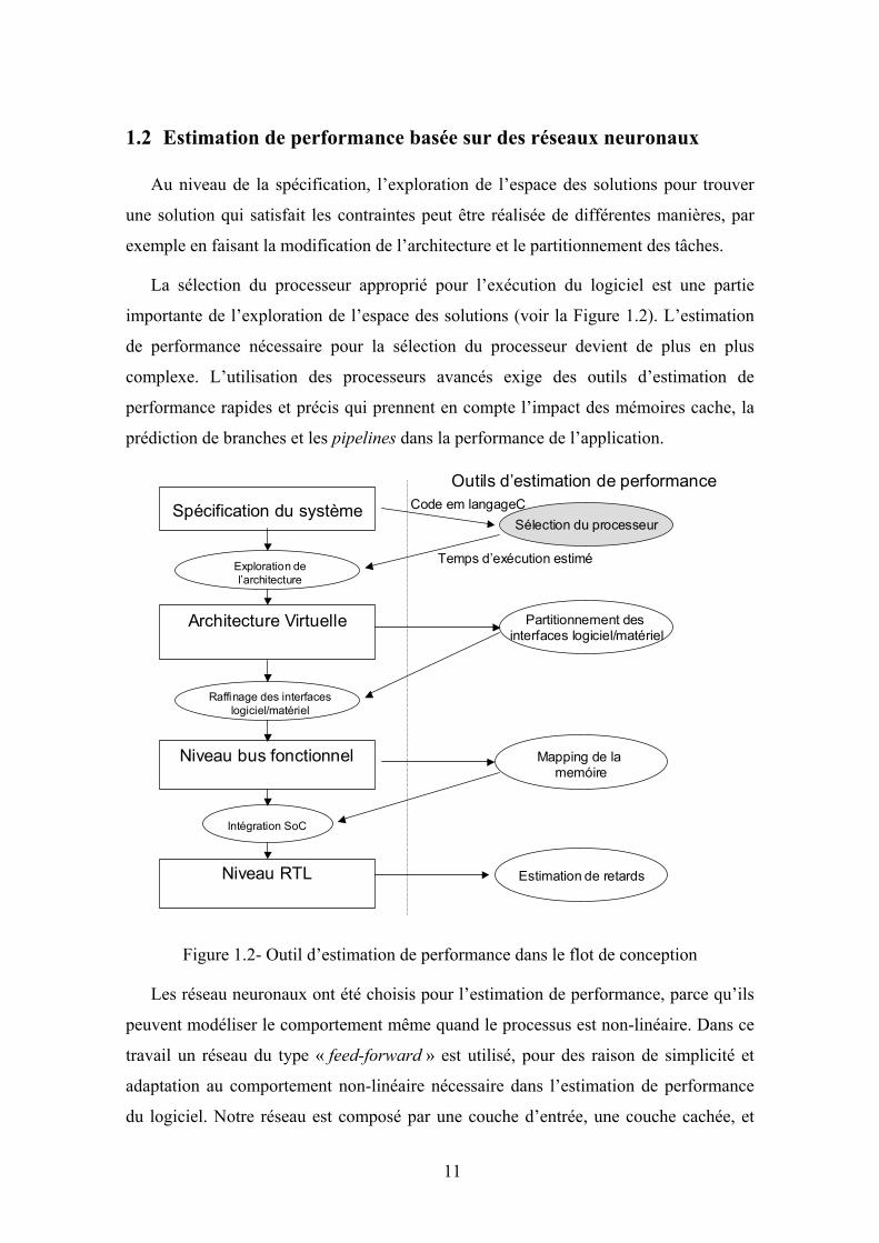
1.2 Estimation de performance basée sur des réseaux neuronaux

Au niveau de la spécification, l’exploration de l’espace des solutions pour trouver

une solution qui satisfait les contraintes peut être réalisée de différentes manières, par

exemple en faisant la modification de l’architecture et le partitionnement des tâches.

La sélection du processeur approprié pour l’exécution du logiciel est une partie

importante de l’exploration de l’espace des solutions (voir la Figure 1.2). L’estimation

de performance nécessaire pour la sélection du processeur devient de plus en plus

complexe. L’utilisation des processeurs avancés exige des outils d’estimation de

performance rapides et précis qui prennent en compte l’impact des mémoires cache, la

prédiction de branches et les pipelines dans la performance de l’application.



Intégration SoC

Niveau RTL









Code em langageC

Temps d’exécution estimé

Figure 1.2- Outil d’estimation de performance dans le flot de conception

Les réseau neuronaux ont été choisis pour l’estimation de performance, parce qu’ils

peuvent modéliser le comportement même quand le processus est non-linéaire. Dans ce

travail un réseau du type « feed-forward » est utilisé, pour des raison de simplicité et

adaptation au comportement non-linéaire nécessaire dans l’estimation de performance

du logiciel. Notre réseau est composé par une couche d’entrée, une couche cachée, et

12

une couche de sortie. Chaque couche peut avoir différents nombres de neurones, et

chaqu’une avoir une fonction de transfert différente.

Notre méthode d’estimation suit deux étapes : entraînement et utilisation. Dans

l’étape d’entraînement, un ensemble de benchmarks sont présentés au réseau neuronal.

Dans cette étape, les entrées sont le nombre d’instructions exécutées classifiées par type

(par exemple branches, arithmétiques et accès à la mémoire), et la sortie attendue est le

nombre de cycles consommés par l’exécution de l’application. Un simulateur précis au

niveau cycle est nécessaire pour obtenir le nombre d’instructions exécutées et les cycles

consommés par l’application. Pour chaque processeur, on a choisi un petit nombre de

classes d’instructions qui représentent le comportement temporel de tous les types

d’instructions.

La Figure 1.3 montre la phase d’entraînement en détail. Dans l’étape 1, un

simulateur précis au niveau cycle est utilisé et les instructions exécutées sont classifiées

par type (étape 2). Dans les étapes 3 et 4 un processus d’apprentissage, basé sur

l’algorithme « back-propagation », permet de changer les poids, de façon à adapter le

réseau pour sortir la valeur désirée. La phase d’entraînement est réalisée en utilisant le

logiciel Matlab.

Classification des instructions

Type Nombre des exécutions

LD/ST n1

INT n2

FLOAT n3

BRANCH n4

Comparer lecycle estiméavec la valeurréelle etchanger lespoids

Profilage d’un ensemble debenchmarks avec unsimulateur précis auniveau cycle

1 2

3

4

Figure 1.3- Étapes d’entraînement du estimateur

Après la phase d’entraînement, l’estimateur de performance est prêt pour être utilisé

dans les projets postérieurs. La Figure 1.4 présente les principales étapes de la phase

d’utilisation. Pour estimer la performance, il est nécessaire de compiler l’application

13

pour le processeur cible, et d’obtenir les instructions exécutées en utilisant un

simulateur fonctionnel. Les instructions classifiées sont présentées comme entrée au

réseau, de sorte qu’il peut estimer le nombre des cycles consommés par l’application.

Cycles estimés

Type Nombre des exécutions

LD/ST n1

INT n2

FLOAT n3

BRANCH n4

Classification des instructions

Comptage dynamique d’instructions

mov R2, R1 load R1, [R3] add R5, R4, R3 .. .. .. .. .. .. store R1, [R3] .. ..

Figure 1.4- La phase d’utilisation de l’estimateur

La Figure 1.5 montre le réseau neuronal utilisé pour estimer la performance dans le

processeur PowerPC750. La couche d’entrée est composée par des neurones avec des

fonctions de transfert linéaires et la couche cachée utilise 5 neurones avec des fonctions

de transfert non-linéaires (tansig). La couche de sortie utilise aussi une fonction de

transfert linéaire. On a utilisé ces neurones en raison de la non-linéarité nécessaire pour

le processus d’estimation. Dans les expériences avec des autres configurations, celle-ci

a donné de meilleurs résultats.

Figure 1.5- Le réseau neuronal pour le processeur PowerPC750 et les fonctions de

transfert

Pour chaque architecture un estimateur différent est créé. Pour cette raison, la

méthode proposée est adaptée pour l’exploration de l’espace de solutions de la partie

logicielle, par exemple quand on veut évaluer les alternatives algorithmiques et de

partionnement des tâches entre les processeurs, parce que des modifications

architecturales demandent un nouveau entraînement.

14

1.3 L’analyse intégrée de performance des systèmes MPSoC

Après le raffinement des interfaces matérielles et logicielles un modèle au niveau du

bus fonctionnel est généré par l’environnent ROSES. Dans le modèle de bus

fonctionnel, les composants matériels sont décrits par les modèles SystemC et les

composants logiciels par tâches compilés pour l’architecture cible. La communication et

synchronisation de la partie logicielle est implémentée par un système d’exploitation

dédié.

Pour analyser la performance d’un système au niveau BFM (voir la Figure 1.6), on

propose l’intégration de deux outils dans le flot ROSES. Le premier est l’environnement

FlexPerf développé chez STMicroelectronics pour l’analyse de performance de logiciel

embarqué. Le deuxième outil est l’environnement MaxSim, utilisé dans le

développement des prototypes virtuels.



Intégration SoC

Niveau RTL









Modèle de simulation

Temps d’exécution en utilisant le prototype virtuel

Figure 1.6- Estimation de performance pour le projet de MPSoC

L’environnement FlexPerf (PAOLI; GALIX; SANTANA, 2004) permet l’analyse

de performance en utilisant une librairie de classes pour l’instrumentation et la

génération des événements de performance. FlexPerf fournit un flot pour générer des

15

modèles de simulation des processeurs qui supportent l’analyse de performance de

logiciel embarqué. L’intégration avec l’environnement ROSES a permis de générer des

modèles de simulation multiprocesseurs en SystemC, avec le support de FlexPerf pour

analyser la performance.

L’environnement MaxSim (ARM, 2007) a été intégré dans le flot ROSES pour

générer un prototype virtuel. La génération du prototype virtuel est réalisée de façon

automatique à partir du modèle de bus fonctionnel utilisé dans l’environnement ROSES.

16

2 ÉTUDE DE CAS DE L’ENCODEUR MPEG4

Dans cette section l’estimation de performance d’un encodeur MPEG4 sera

présentée en utilisant les outils d’estimation développés dans cette thèse. L’architecture

MPEG4 proposé par Bonaciu et al. (2006), est une implémentation parallèle développée

pour fournir la flexibilité et le support à des différents profils.

VLC

Fn

CodedImage

VLC Task (SW)

DCT Quant

IDCT

IntraPrediction

ImageReconstruct

MotionEstimation

Fn-1

Encoder Task (SW)

MotionComp.

InputCombiner

Rate control

DMA

DeQuant

Figure 2.1- L’architecture de l’encodeur MPEG4 (Bonaciu et al., 2006)

L’encodeur MPEG4 est composé de cinq composants, comme montre la Figure

2.1 :

- Input: ce composant est responsable pour recevoir l’image d’entrée et

l’envoyer à la tâche Encodeur ;

- Encoder task : cette tâche exécute la partie principale de l’encodage

MPEG4 ;

- VLC task: cette tâche réalise la compression de l’image en utilisant

l’algorithme d’Huffman ;

- Combiner: ce composant prépare le résultat final de la compression de

l’image;

17

- DMA (Direct memory access): ce composant matériel est responsable pour

réaliser tous les transferts parmi les composants de l’architecture MPEG4.

La Figure 2.1 montre l’encodeur MPEG4 avec deux processeurs. Le premier

exécute la tâche d’encodage et le deuxième est responsable pour exécuter la tâche VLC.

Le composant DMA fait les transferts parmi les composants de l’architecture. Le flot

d’exécution de l’encodeur commence par le chargement de l’image dans le processeur

Encoder par le composant Input. Après l’encodage, les données sont transférées au

processeur VLC. Après la compression par la tâche VLC, les donnés compressées sont

envoyées vers l’unité de stockage par le composant Combiner.

2.1 Flot d’estimation et analyse de performance

Dans l’analyse de l’encodeur MPEG4, le flot de conception montré dans la

Figure 2.2 sera réalisé. A partir de la spécification du système décrit en langage C,

l’estimation de performance sera réalisée en utilisant l’estimateur basé sur des réseaux

neuronaux. Dans l’étude de cas seulement les composants logiciels Encoder et VLC

seront utilisés dans l’analyse de performance.

La première étape d’estimation est utilisée pour guider la sélection du processeur

qui sera responsable pour l’exécution des composants logiciels. Dans cette étape, deux

processeurs sont évalués : ARM946 et PowerPC750. L’objectif de cette étape est

d’évaluer rapidement la performance telle que le processeur plus efficace soit utilisé.

La sélection du processeur affecte les étapes subséquentes dans le flot de

conception, car les interfaces matérielles et logicielles sont assemblées pour une

architecture spécifique. Le raffinement des interfaces matérielles et logicielles est

réalisé par l’environnement ROSES, où le modèle de bus fonctionnel est généré. Dans

ce travail l’architecture virtuelle ne sera pas utilisée pour l’estimation de performance.

D’autres travaux au sein du groupe TIMA, comme ceux proposés par Aimen

Bouchhima (2005), utilisent l’architecture virtuelle pour faire l’estimation de

performance en utilisant un modèle abstrait de processeur.

Pour analyser la performance au niveau du bus fonctionnel, le prototype virtuel

est généré automatiquement à partir de la description de ROSES. Pour la génération du

prototype virtuel, on considère que les composants matériels sont décrits en SystemC au

18

niveau du cycle. Le logiciel est organisé en tâches et exécute sur un système

d’exploitation spécifique pour l’application. Le prototype virtuel est généré dans

l’environnement MaxSim.

Architecture virtuelle(TLM)

CPU et matériel abstraits


ROSESRaffinage des

Interfaces

VM1 VM2

VM3 HW

Appl.

Adaptateur

CPU Matériel

Réseau d’interconnexion

CPU

Adaptateur Adaptateur

Appl.

Système d’exploitation


Explorationde l’architecture

f1f2

f3f4 Sélection du

processeur pour les composants logiciels en utilisant réseau neuronal

Prototype virtuel: Analyse de performance intégrée matériel et logiciel

(a)

(b)

(c)

Système d’exploitation

Figure 2.2 - Flot de conception et estimation de performance en systèmes MPSoC

2.2 Estimation au niveau de la spécification

Dans la première étape, on utilise l’estimateur haut niveau pour évaluer la

performance des composants logiciels. Dans cette étude de cas, les tâches Encoder et

VLC sont évaluées. Malgré la simplification de l’architecture avec deux processeurs, la

sélection du processeur est un aspect important dans l’exploration de l’espace des

solutions.

Dans les expériences, deux processeurs sont utilisés: ARM946 et PowerPC750.

Ceux-ci ont certaines caractéristiques comme pipeline et mémoire cache qui rendent

difficile l’estimation de leurs performances.

Le réseau neuronal nécessite un entraînement pour calibrer l’estimateur. Un

ensemble de 41 benchmarks est utilisé pour entraîner et tester la précision de

l’estimateur. La Figure 2.3 montre le réseau neuronal utilisé pour estimer la

19

performance du processeur ARM946, où les entrées sont le nombre d’instructions

exécutées par l’application (classifiées par type).

InputLayer

HiddenLayer

OutputLayer

Forward Branches

Backward Branches

Load/Store

Multiple Load/Store

ALU

Cycles

Figure 2.3- L’estimateur pour le processeur ARM946

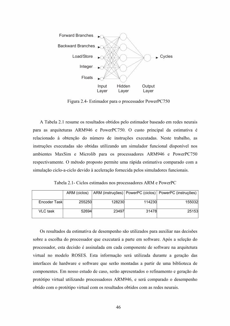
Pour chaque processeur, un ensemble de types d’instructions est choisi de telle

façon qu’il représente la performance de l’application. Dans le cas du processeur

PowerPC750, les instructions sont classifiées comme : branchement arrière,

branchement avant, load/store, opérations entières et opération flottantes, comme

montre la Figure 2.4.

Pour l’entraînement du réseau neuronal, un simulateur précis au niveau du cycle

est nécessaire pour obtenir les instructions exécutées et les cycles consommés. Pour le

processeur ARM946, le simulateur fournit dans l’environnement MaxSim (ARM, 2007)

est utilisé, et pour le processeur PowerPC 750 on utilise le simulateur Microlib (2007).

InputLayer

HiddenLayer

OutputLayer

Forward Branches

Backward Branches

Load/Store

Integer

Floats

Cycles

Figure 2.4- L’estimateur pour le processeur PowerPC750

Le Tableau 2.1 résume les résultats de l’estimation obtenus par l’estimateur basé

sur des réseaux neuronaux, pour les architectures PowerPC750 et ARM946. Le coût de

20

l’estimation est principalement du à l’obtention du nombre d’instructions exécutées.

Dans ce travail, les instructions exécutées sont obtenues en utilisant les simulateurs

fonctionnels disponibles dans l’environnement MaxSim et Microlib pour le processeur

ARM946 et PowerPC750 respectivement. La méthode proposée permet une estimation

rapide en raison de l’accélération fournie par des simulateurs fonctionnels.

Tableau 2.1- Cycles estimés dans les processeurs ARM946 et PowerPC750

ARM (cycles) ARM (instructions) PowerPC (cycles) PowerPC (instructions)

Encoder Task 255250 128230 114230 155032

VLC task 52694 23497 31478 25153

Les résultats de l’estimation sont utilisés pour aider les décisions sur la sélection

du processeur qui exécutera la partie logiciel. Après la sélection du processeur, cette

décision est signalée a chaque composant logiciel de l’architecture virtuelle dans le

modèle ROSES. Cette information sera utilisée pendant la génération des interfaces

matérielles et logicielles qui sont assemblées à partir d’une librairie de composants.

Dans notre étude de cas, on va démontrer la génération du prototype virtuel pour le

processeur ARM946, et comparer la performance obtenue avec le prototype virtuel avec

les résultats de l’estimation basée sur des réseaux neuronaux.

2.3 Analyse de performance avec un prototype virtuel

Après la génération des interfaces matérielles et logicielles on utilise un

prototype virtuel pour valider et analyser la performance du système au niveau du bus

fonctionnel. L’environnement MaxSim (ARM, 2007) est utilisé pour générer le

prototype virtuel, permettant l’évaluation de performance. Les composants matériels

sont considérés comme blocs IP (intellectual property) en SystemC. Les interfaces

matérielles générées par ROSES sont déjà disponibles comme les blocs SystemC. Les

composants SystemC sont encapsulés dans les composants Maxsim, puisque les

composants sont disponibles pour la simulation. Les composants logiciels avec le

système d’exploitation sont compilés pour l’architecture cible et chargés dans la

mémoire pendant l’initialisation de la simulation.

21

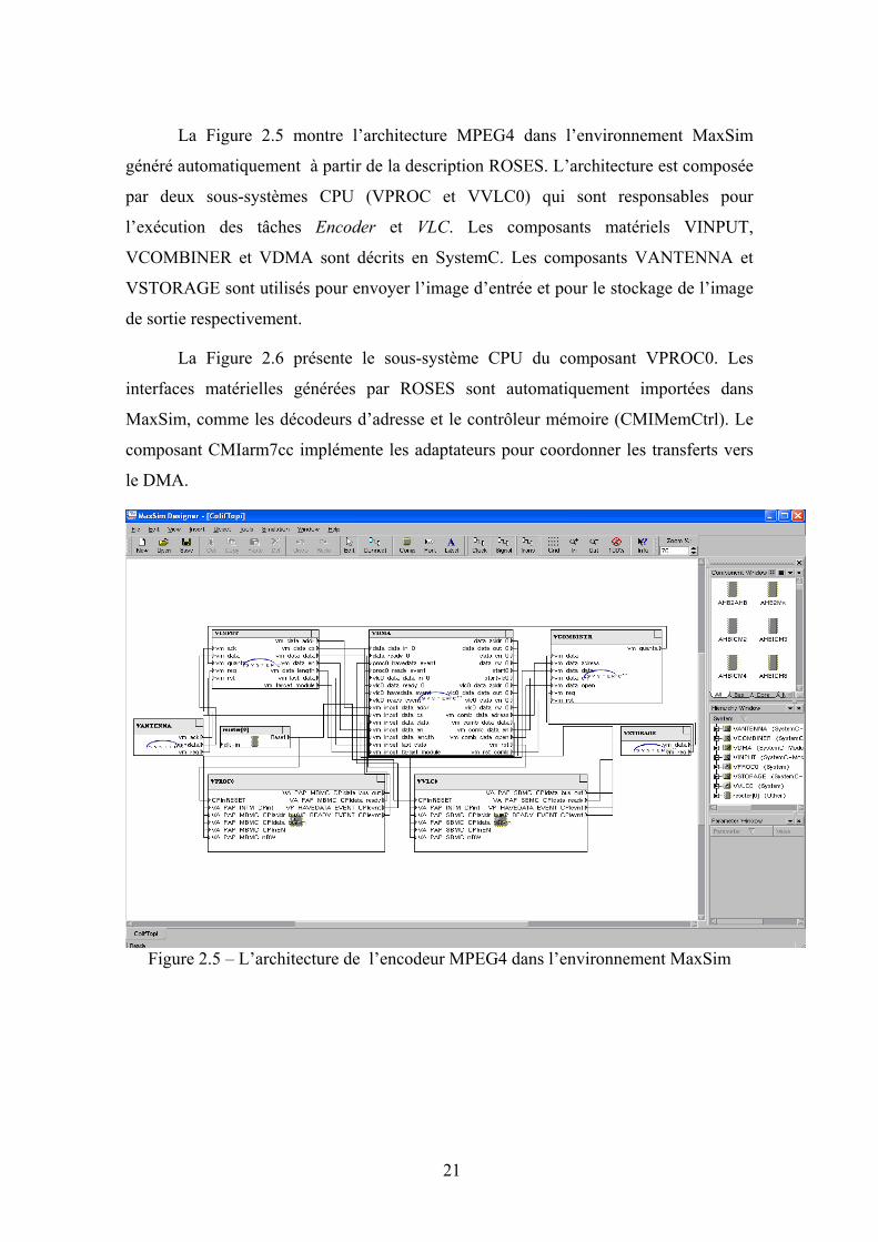
La Figure 2.5 montre l’architecture MPEG4 dans l’environnement MaxSim

généré automatiquement à partir de la description ROSES. L’architecture est composée

par deux sous-systèmes CPU (VPROC et VVLC0) qui sont responsables pour

l’exécution des tâches Encoder et VLC. Les composants matériels VINPUT,

VCOMBINER et VDMA sont décrits en SystemC. Les composants VANTENNA et

VSTORAGE sont utilisés pour envoyer l’image d’entrée et pour le stockage de l’image

de sortie respectivement.

La Figure 2.6 présente le sous-système CPU du composant VPROC0. Les

interfaces matérielles générées par ROSES sont automatiquement importées dans

MaxSim, comme les décodeurs d’adresse et le contrôleur mémoire (CMIMemCtrl). Le

composant CMIarm7cc implémente les adaptateurs pour coordonner les transferts vers

le DMA.

Figure 2.5 – L’architecture de l’encodeur MPEG4 dans l’environnement MaxSim

22

SystemC modules generated by ASAG

Figure 2.6– Sous-système CPU du composant VPROC0

Pour simuler la CPU, un modèle de bus fonctionnel a été implémenté en utilisant

des processeurs, des mémoires et le bus disponibles dans la librairie MaxSim. La Figure

2.7 présente le modèle de bus fonctionnel basé sur un processeur ARM9. Le processeur

est connecté à la mémoire en utilisant des interfaces TLM. L’intégration avec le reste du

système est réalisée par un adaptateur (mem_adapter) qui permet la communication des

interfaces TLM avec des interfaces au niveau des portes.

Figure 2.7- Modèle de simulation du processeur

23

Figure 2.8- Écran de simulation de l’environnement MaxSim

MaxSim Explorer est utilisé pour simuler le système. La Figure 2.8 montre

l’écran de simulation. Pendant l’initialisation de la simulation, les fichiers avec les

binaires de l’application et le système d’exploitation sont présentés.

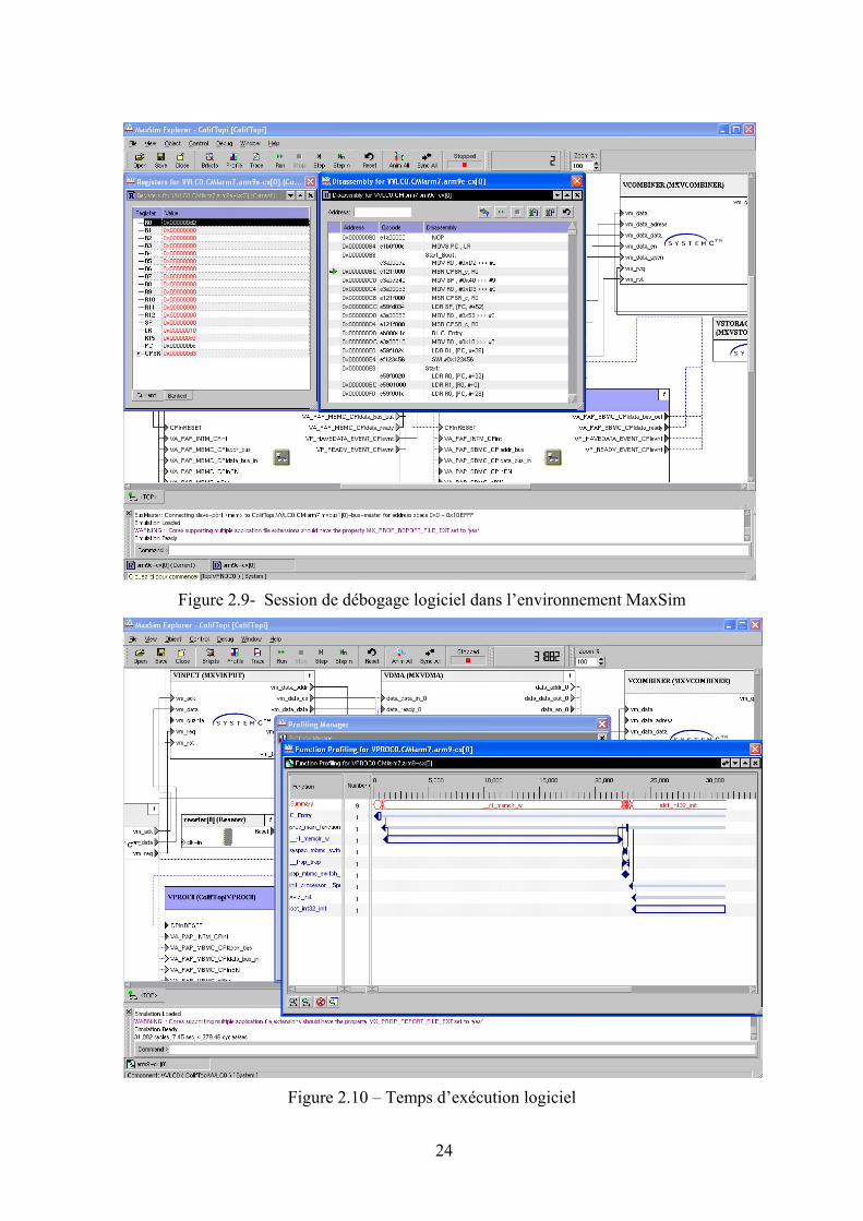
L’environnement MaxSim fournit un support pour la validation globale, en

utilisant des points d’arrêt sur de code logiciel, registres, positions de mémoire et

connections. La Figure 2.9 présente l’écran avec le code assembleur du processeur

VVLC0. L’environnement supporte le déboguage pour tous les processeurs, facilitant la

validation des applications qui exécutent en architectures MPSoC.

La Figure 2.10 montre le temps d’exécution du logiciel divisé par fonctions dans

le processeur VPROC0. Ce type d’analyse permet la détection de points d’optimisations

et quelles sont les fonctions qui prennent plus de temps dans l’exécution de

l’application.

24

Figure 2.9- Session de débogage logiciel dans l’environnement MaxSim

Figure 2.10 – Temps d’exécution logiciel

25

Le Tableau 2.2 présente les résultats de l’estimation de performance avec réseau

neuronal comparés avec ceux obtenus par le prototype virtuel. Pour le processeur

PowerPC750, un simulateur SystemC précis au niveau du cycle a été utilisé. Bien que

cette simplification limite l’analyse de performance, le simulateur permet de vérifier la

précision de l’estimateur basé sur des réseaux neuronaux. Pour le processeur ARM946,

l’erreur d’estimation a été de 4.26% pour la tâche Encoder et de -8.29% pour la tâche

VLC. Pour le processeur PowerPC750 une erreur de 21% est obtenue pour la tâche

Encodeur. L’erreur pour le processeur PowerPC750 est légèrement plus grande en

raison de la complexité du processeur.

On compare notre méthode avec l’estimation basée sur la régression linéaire

proposée par Giusto et al. (2001). Dans le cas du processeur ARM946, la régression

linéaire donne des erreurs d’estimation de 60.25% et 58.66% pour les tâches Encoder et

VLC respectivement, ce qui démontre la flexibilité et la prédiction non linéaire de

l’estimateur basé sur des réseaux neuronaux.

Tableau 2.2- Comparaison de précision de l’estimateur de performance et le prototype

virtuel

ARM946 PowerPC750

Estimé Cycle précis Erreur Estimé Cycle précis Erreur

Encoder

Task 255250 266630 4.26% 114230 151960 24.8%

VLC Task 52694 48659 -8.29% 31478 31064 1.33%

Le Tableau 2.3 présente les temps nécessaires (en secondes) pour l’estimation et

l’exécution du prototype virtuel. L’estimation basée sur des réseaux neuronaux permet

une accélération considérable par rapport à la simulation en utilisant le prototype

virtuel. Les réseaux neuronaux permettent une estimation rapide qui est important en

raison de l’augmentation de la partie logicielle dans les systèmes embarqués. De l’autre

coté, le prototype virtuel fournit une solution globale d’analyse intégrée des composants

matériels et logiciel qui permet la confirmation des valeurs estimées au haut niveau

d’abstraction.

26

Tableau 2.3 – Temps de simulation avec le prototype virtuel et l’estimateur des réseaux

neuronaux

ARM946 PowerPC750

Cycle

précis(s)

Estimation

(s)

Accélération Cycle

précis (s)

Estimation

(s)

Accélération

Encoder Task 5.5 0.3 22.0 4.3 0.3 14.3

VLC Task 3.0 0.2 14.3 1.4 0.2 6.5

27

3 CONCLUSIONS

Dans cette thèse, on propose une méthodologie intégrée pour la conception et

l’estimation de performance dans les systèmes multiprocesseurs monopuces (MPSoC),

où le support pour l’estimation de performance est fournit pendant le flot de conception.

L’environnement ROSES développé au sein du groupe TIMA est utilisé comme flot de

conception et intégré avec les outils de performance proposés dans cette thèse.

Au niveau de la spécification, on propose l’utilisation des estimateurs

analytiques pour guider la sélection du processeur qui permettent une estimation rapide

et précise. Les réseaux neuronaux sont utilisés comme estimateurs en raison de la

flexibilité et l’adaptation non linéaire nécessaires pour l’estimation aux processeurs

d’architectures complexes. Les résultats de l’utilisation des réseaux neuronaux comme

estimateurs ont été présentés dans un article (OYAMADA et al., 2004) à la conférence

SBCCI.

On propose l’utilisation de méthodes basées sur la simulation pour analyser la

performance au niveau de bus fonctionnel. Dans ce travail, deux outils de performance

sont intégrés dans le flot de conception ROSES.

Dans le premier, l’environnement FlexPerf développé pour l’analyse de

performance des logiciels embarqués a été intégré dans le flot ROSES. Le simulateur de

processeur avec le support à l’analyse de performance disponible dans l’environnement

FlexPerf est intégré dans le modèle de simulation en SystemC généré par ROSES. Cette

intégration a apportée le support à l’instrumentation et l’analyse de performance fournit

par l’environnement FlexPerf.

Le deuxième outil intégré dans le flot ROSES est l’environnement de prototype

virtuel MaxSim. Pour créer le prototype virtuel, un outil a été implémenté qui génère

automatiquement dans MaxSim un prototype virtuel a partir du modèle de bus

fonctionnel. Pour l’exécution de la partie logicielle les simulateurs précis au niveau

28

cycle disponibles dans MaxSim sont utilisés. Le prototype virtuel fournit un modèle de

validation global qui permet le débogage des applications dans l’architecture MPSoC.

Pour valider les outils d’estimation de performance développés dans cette thèse

une étude de cas d’un encodeur multiprocesseur MPEG4 a été démontrée. Cette plate-

forme impose quelques défis pour l’analyse de performance comme les multiples

processeurs et des composants de propriété intellectuel. L’étude de cas a permis

d’évaluer l’estimation de performance haut niveau et de comparer la précision avec le

prototype virtuel. Ce travail a été publié dans la conférence ASPDAC (OYAMADA et

al. 2007).

3.1 Limitations des méthodes proposées et les perspectives

À partir des résultats obtenus dans le développement de l’étude de cas, quelques

limitations peuvent être identifiées :

a) La précision du réseau neuronal est dépendante de la qualité des entrées utilisées

dans l’étape d’entraînement. Dans ce travail, l’ensemble d’entraînement a été

sélectionné pour favoriser la généralisation, en utilisant des applications de

différentes tailles et domaines.

b) Pour l’entraînement de l’estimateur, un simulateur précis au niveau du cycle est

nécessaire. Pour l’étape d’utilisation, afin d’obtenir les instructions exécutées un

simulateur fonctionnel est utilisé. L’accélération de la méthode proposée est

dépendante de la vitesse du simulateur fonctionnel;

c) Le prototype virtuel utilise la simulation qui a un coût élevé pour l’exécution de

grandes architectures avec nombreux processeurs. Dans ce cas, le prototype

virtuel peut être utilisé pour analyser l’initialisation ou seulement des parties

spécifiques du code.

Malgré les contributions obtenues dans ce travail, quelques perspectives potentielles

sont identifiées :

a) L’étude de l’application des réseaux neuronaux pour l’estimation de energie ;

b) L’utilisation de paramètres architecturaux dans le réseau neuronal, comme

proposé par Ipek (2006) ;

29

c) L’utilisation d’un outil de profilage générique et la traduction pour le processeur

cible, pour remplacer le simulateur fonctionnel utilisé dans l’étape d’estimation

du réseau neuronal ;

d) L’intégration de la méthode d’estimation proposée dans ce travail avec autres

langages de spécification comme UML et Simulink;

e) La génération du prototype virtuel avec canaux au niveau transactionnel (TLM),

pour fournir une simulation plus rapide.

30

BIBLIOGRAPHIE

ARM – MaxCore. Disponible à <http://www.arm.com >, 2007.

BONACIU, M.; BOUCHHIMA, A.; YOUSSEF, W.; CHEN, X.; CESARIO, W.;

JERRAYA, A.A. High-Level Architecture Exploration for MPEG4 Encoder with

Custom Parameters. In: ASIAN AND SOUTH PACIFIC DESIGN AUTOMATION

CONFERENCE, ASP-DAC, 11th, 2006, Yokohama, Japan. Proceedings... New York:

ACM Press, 2006. p.372-377.

BOUCHHIMA, A.; BACIVAROV, I.; YOUSSEF, W.; BONACIU, M.; JERRAYA,

A.A. Using Abstract CPU Subsystem Simulation Model for High Level HW/SW

Architecture Exploration. In: ASIAN AND SOUTH PACIFIC DESIGN

AUTOMATION CONFERENCE, ASP-DAC, 10th, 2005, Shanghai, Chine.

Proceedings... New York: ACM Press, 2005. p.18-25.

GIUSTO, P.; MARTIN, G.; HARCOURT, E. Reliable Estimation of Execution

Time of Embedded Software. In: DESIGN AUTOMATION AND TEST IN EUROPE,

DATE, 2001, Munich, Germany. Proceedings…IEEE Computer Society Press, 2001.

p. 580-585.

IPEK; E. MACKKE; S. SUPINSKI; B. SCHULZ; M. CARUANA; R. Efficiently

Exploring Architecture Design Spaces via Predictive Modeling. In: INTERNATIONAL

CONFERENCE ON ARCHITECTURAL SUPPORT FOR PROGRAMMING

LANGUAGES AND OPERATING SYSTEMS, ASPLOS, 2006, San Jose, USA.

Proceedings… ACM Press, 2006. p. 195-206.

MEYEROWITZ, T.; KISHINEVSKY, M.; KAM, T.; LAVAGNO, L.;

SANGIOVANNI-VINCENTELLI, A. Modeling Microarchitectural Performance using

31

Metropolis: Performance Estimation and Back-Annotation. Technical Report. July,

2004. http://www.eecs.berkeley.edu/~tcm/projects.html.

MicroLib –PPC 750. Disponible à <http://microlib.org>, 2007.

OYAMADA, M.S.; CESARIO, W.; BONACIU, M.; WAGNER, F.R.; JERRAYA,

A. Software Performance Estimation in MPSoC Design. In: ASIAN AND SOUTH

PACIFIC DESIGN AUTOMATION CONFERENCE. ASP-DAC, 12th, 2007,

Yokohama, Japan. Proceedings… IEEE Press, 2007. p. 38- 43.

OYAMADA, M.S.; ZSCHONARCK, F.; WAGNER, F.R. Accurate Software

Performance Estimation Using Domain Classification and Neural Networks. In:

SYMPOSIUM ON INTEGRATED CIRCUITS AND SYSTEMS DESIGN. SBCCI,

17th, 2004, Porto de Galinhas, Brazil. Proceedings... ACM Press, 2004. p. 175-180.

PAOLI, S.; GALIX, E.; SANTANA, M. FlexPerf: A performance evaluation framework for embedded software and architectures. ST Journal of Research. v. 1, n. 2, p. 17- 31, September 2004.

33

ANNEXE A ESTIMATIVA DE DESEMPENHO DE SOFTWARE EMBARCADO EM SISTEMAS MULTIPROCESSADOS INTEGRADOS EM CHIP

Marcio Seiji OYAMADA Laboratoire TIMA – INPG

LSE Lab - UFRGS

34

1 ESTIMATIVA DE DESEMPENHO DO PROJETO DE MULTIPROCESSADORES INTEGRADOS EM CHIP

O aumento na capacidade de integração de transistors permite o desenvolvimento

de soluções compostas por vários processadores, componentes de aplicação específica e

interfaces digitais e analógicas em um único chip. Atualmente, constata-se o aumento de

soluções com vários processadores em um único chip, denominadas MPSoC (sistemas

multiprocessados em único chip- multiprocessor system-on-chip). Em comparação com

soluções puramente em hardware, a utilização de processadores fornece a flexibilidade e

heterogeneidade necessária em sistemas embarcados.

O projeto de um sistema embarcado é guiado por requisitos de projetos restritos. O

fluxo de projeto de um MPSoC necessita de ferramentas para verificar se os requisitos

estão sendo satisfeitos. O desempenho é normalmente o principal critério adotado para

guiar a exploração da arquitetura. No entanto, outros aspectos precisam ser avaliados

nos estágios iniciais do projeto, tais como potência consumida, energia e área.

A estimativa de desempenho é um processo contínuo e pode ser aplicada em

diferentes níveis de abstração como apresentado na Figura 1.1. Durante a especificação

do sistema, a estimativa de desempenho auxilia no particionamento das funcionalidades

em componentes de hardware e software, a seleção do processador, e a atribuição de

tarefas entre os processadores.

A arquitetura virtual é um modelo onde o software ainda não foi mapeado para o

processador alvo e a comunicação é realizada utilizando transações. Como a

interconexão ainda não está definida, neste nível é possível explorar as diferentes

possibilidades de mapeamento dos canais no nível de transações (TLM - transaction

level model), na estrutura de comunicação.

No nível funcional do barramento (BFM- bus functional model) as interfaces de

hardware e software já estão refinadas e o software é compilado para o processador

35

alvo. Neste nível, o detalhamento das interfaces e do sistema operacional possibilita

uma análise precisa do desempenho do hardware e software.

Virtual ArchitectureModel at TLM Level

BFM Level

SoC Integration

RTL Level

Performance Estimation Tools

HW/SW interface refinement

System Specification

Architecture exploration

Processor Selection

HW/SW InterfacePartitioning

Memory mapping

Delay estimation

Scope of this work

Figura 1.1- Ferramentas de estimativa de desempenho nos diferentes níveis de

apresentação

Devido ao aumento na utilização de processadores nos projetos de MPSoC, e como

conseqüência o crescimento da parte em software, ferramentas para estimativa de

desempenho em software precisam ser desenvolvidas. Ferramentas de estimativa de

desempenho podem ser divididas em três grupos: simulação, modelos abstratos e

anotação do código (MEYEROWITZ, 2004). Métodos baseados em simulação utilizam

simuladores com precisão de ciclos para estimar o tempo de execução. Modelos

abstratos ou analíticos utilizam funções de custo para calcular o tempo de execução do

software. Métodos no nível intermediário são baseados na anotação do código com

custo de execução. Desta forma, a aplicação executa nativamente, sendo vantajoso em

relação à simulação ciclo-a-ciclo devido a rapidez na obtenção dos ciclos consumidos

pela aplicação.

36

Devido ao aumento do número de processadores e também as possíveis variações na

interconexão entre os mesmos, a análise isolada do desempenho do software torna-se

altamente imprecisa. Desta forma, um modelo de estimativa de desempenho integrado

de hardware e software é necessário.

Este trabalho propõe métodos para a estimativa de desempenho, que são necessários

devido ao grande espaço de projeto que não pode ser explorado manualmente ou

verificado somente quanto um protótipo de hardware esteja disponível. Considerando o

aumento da complexidade dos processadores utilizados em sistemas embarcados, é

necessário que as ferramentas de estimativa de desempenho possam estimar o

desempenho neste tipo de arquitetura. Neste trabalho, um modelo analítico de

estimativa de desempenho baseado em redes neurais é proposto. Por outro lado,

ferramentas de estimativa de desempenho que considerem de forma integrada os

componentes de hardware e software do sistema é necessário. Este trabalho apresenta a

utilização de protótipos virtuais como forma de avaliar o desempenho do sistema no

nível BFM, que provêem um modelo global de simulação, permitindo a avaliação

conjunta do desempenho dos componentes de hardware e software.

1.1 Integração de estimativa de desempenho no projeto de MPSoC

Esta tese propõe uma metodologia para a análise e estimativa de desempenho em

sistemas multiprocessados integrados em única pastilha (MPSoC- multiprocessor

system-on-chip). Neste trabalho o ambiente ROSES é utilizado para guiar o fluxo de

estimativa de desempenho. O ambiente ROSES utiliza um paradigma baseado em

componentes para refinar as interfaces de hardware e software em um MPSoC,

utilizando como entrada uma arquitetura virtual composta de módulos de hardware e

software interconectada por canais TLM. Os componentes de hardware são

considerados como caixa-preta, onde somente a interface é conhecida. Os componentes

em software são modelados como um conjunto de tarefas, que são mapeadas para os

processadores na arquitetura.

Neste trabalho, um método para estimar rapidamente o desempenho do software

baseado em redes neurais é proposto para guiar a seleção de processadores. Redes

neurais se mostraram uma solução adequada para modelar o comportamento não linear

do software executando em um processador com recursos avançados tais como pipeline,

37

caches, predição de desvios entre outros. Experimentos realizados com diferentes

arquiteturas tais como PowerPC 750, DSP, ARM, e um processador Java, mostraram a

flexibilidade de redes neurais para utilização na estimativa de estimativa de desempenho

do software.

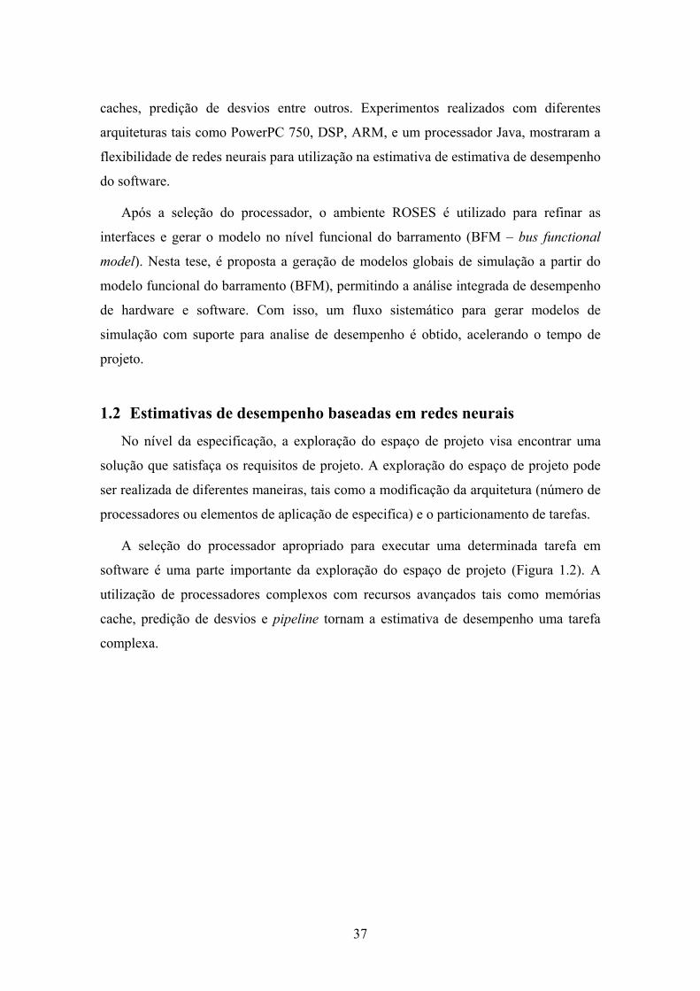
Após a seleção do processador, o ambiente ROSES é utilizado para refinar as

interfaces e gerar o modelo no nível funcional do barramento (BFM – bus functional

model). Nesta tese, é proposta a geração de modelos globais de simulação a partir do

modelo funcional do barramento (BFM), permitindo a análise integrada de desempenho

de hardware e software. Com isso, um fluxo sistemático para gerar modelos de

simulação com suporte para analise de desempenho é obtido, acelerando o tempo de

projeto.

1.2 Estimativas de desempenho baseadas em redes neurais

No nível da especificação, a exploração do espaço de projeto visa encontrar uma

solução que satisfaça os requisitos de projeto. A exploração do espaço de projeto pode

ser realizada de diferentes maneiras, tais como a modificação da arquitetura (número de

processadores ou elementos de aplicação de especifica) e o particionamento de tarefas.

A seleção do processador apropriado para executar uma determinada tarefa em

software é uma parte importante da exploração do espaço de projeto (Figura 1.2). A

utilização de processadores complexos com recursos avançados tais como memórias

cache, predição de desvios e pipeline tornam a estimativa de desempenho uma tarefa

complexa.

38


BFM Level

SoC Integration

RTL Level





Processor Selection


OS overhead,Memory mapping

Delay estimation

C code

Estimated software execution time

Simulation model

SW execution time in a cycle accurate

Simulation model

Communication requirements between the components

Synthetizable RTL model

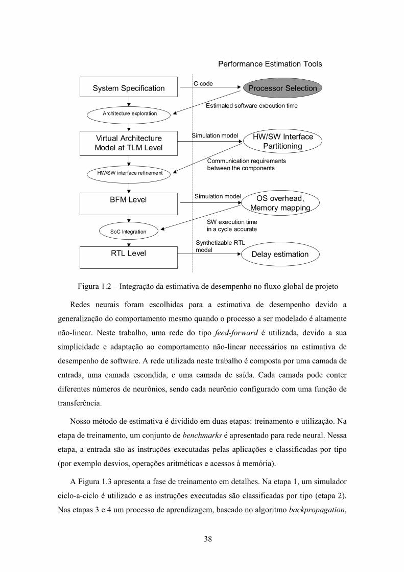
Figura 1.2 – Integração da estimativa de desempenho no fluxo global de projeto

Redes neurais foram escolhidas para a estimativa de desempenho devido a

generalização do comportamento mesmo quando o processo a ser modelado é altamente

não-linear. Neste trabalho, uma rede do tipo feed-forward é utilizada, devido a sua

simplicidade e adaptação ao comportamento não-linear necessários na estimativa de

desempenho de software. A rede utilizada neste trabalho é composta por uma camada de

entrada, uma camada escondida, e uma camada de saída. Cada camada pode conter

diferentes números de neurônios, sendo cada neurônio configurado com uma função de

transferência.

Nosso método de estimativa é dividido em duas etapas: treinamento e utilização. Na

etapa de treinamento, um conjunto de benchmarks é apresentado para rede neural. Nessa

etapa, a entrada são as instruções executadas pelas aplicações e classificadas por tipo

(por exemplo desvios, operações aritméticas e acessos à memória).

A Figura 1.3 apresenta a fase de treinamento em detalhes. Na etapa 1, um simulador

ciclo-a-ciclo é utilizado e as instruções executadas são classificadas por tipo (etapa 2).

Nas etapas 3 e 4 um processo de aprendizagem, baseado no algoritmo backpropagation,

39

altera os pesos dos neurônios, adaptando a rede neural para responder com o valor

desejado. A fase de treinamento é realizada utilizando o software Matlab.

Instruction classification

Type Number of occurrences

LD/ST n1

INT n2

FLOAT n3

BRANCH n4

Compare number of estimated cycles with number of real cycles and adjust the weights

Profile ofbenchmark setand extractionof executedinstructions andcycles

1 2

3

4

Figura 1.3- Treinamento da rede neural

Após a fase de treinamento o estimador de desempenho está pronto para ser

utilizado nos projetos subseqüentes. A Figura 1.4 apresenta as principais etapas da fase

da utilização. Para estimar o desempenho, é necessário compilar a aplicação para o

processador alvo, e obter as instruções executadas utilizando um simulador funcional.

As instruções classificadas são apresentadas como entrada à rede neural para que a

mesma possa estimar o número de ciclos consumidos pela aplicação.


LD/ST n1

INT n2

FLOAT n3

BRANCH n4


Estimated cycles

Dynamic instruction count


Figura 1.4- Fase de utilização da rede neural

A Figura 1.5 apresenta a rede neural utilizada para estimar os ciclos no processador

PowerPC750. A camada de entrada é composta por neurônios com funções de

transferência lineares e a camada escondida é composta por neurônios com funções de

transferência não lineares (tansig). A camada de saída utiliza também uma função de

40

transferência linear. A escolha desses tipos de funções de transferência foi devido ao

comportamento não linear a ser modelado. Os testes com outras configurações, esta

arquitetura resultou nos melhores resultados.

InputLayer

HiddenLayer

OutputLayer

Forward Branches

Backward Branches

Load/Store

Integer

Floats

Cycles

(a) Rede neural (b) Função de transferência

tansig

(c) Função de transferência

linear

Figura 1.5- Rede neural para o processador PowerPC 750 (a), e as funções de

transferência tansig(b) e linear (c)

Para cada arquitetura um estimador diferente é criado. Devido a essa restrição, o

método proposto é eficiente para a exploração do espaço de projeto da parte de

software, com o objetivo para avaliar as alternativas de implementação de algoritmos e

o particionamento de tarefas entre processadores de um conjunto pré-definido de

arquiteturas, visto que modificações arquiteturais necessitam de um novo treinamento.

1.3 Análise de desempenho integrada de hardware e software utilizando modelos de simulação

Após o refinamento das interfaces de hardware e software um modelo no nível

funcional do barramento (BFM) é gerado pelo ambiente ROSES. No modelo BFM, os

componentes em hardware são modelados em SystemC e os componentes de software

são tarefas compiladas para o processador alvo. A comunicação e sincronização das

tarefas em software são realizadas através de um sistema operacional customizado para

a aplicação. Para analisar o desempenho do sistema no nível BFM (Figura 1.6), é

proposto a integração de duas ferramentas no fluxo de projeto ROSES: FlexPerf e

MaxSim.

41


BFM Level

SoC Integration

RTL Level





Processor Selection



Delay estimation

C code


Simulation model

SW execution time in a cycle accurate

Simulation model



Figura 1.6- Integração de protótipos virtuais no ambiente ROSES

O framework FlexPerf (PAOLI; GALIX; SANTANA, 2004), permite a análise de

desempenho através de uma biblioteca que suporta a instrumentação e geração de

eventos em um simulador. O framework provê um conjunto pré-implementado de

módulos de análise de desempenho, possibilitando a extensão e customização das

mesmas. O framework FlexPerf tem fluxo bem definido para gerar modelos de

simulação de processadores utilizando a linguagem LISA, com todo o suporte

necessário para a análise de desempenho do software embarcado. Desta forma, a

integração com o ROSES permitiu a geração de modelos de simulação de uma

arquitetura MPSoC, com suporte para a análise de desempenho. A ferramenta CosimX

foi alterada para gerar modelos SystemC utilizando processadores disponibilizados pelo

FlexPerf. Desta forma, uma arquitetura MPSoC pode ser simulada e o devido suporte

para análise desempenho é fornecida. Neste trabalho, uma arquitetura multiprocessada

de um codificador MPEG4 foi gerada e análise de desempenho do hardware e software

realizada.

42

Uma outra forma de disponibilizar a análise de desempenho no nível funcional do

barramento é a utilização de protótipos virtuais. Neste trabalho, a ferramenta MaxSim

(ARM, 2005) foi integrada ao ambiente ROSES, de forma que um protótipo virtual

possa ser gerado automaticamente a partir de uma descrição da arquitetura. O ambiente

MaxSim provê uma biblioteca de processadores, memórias, barramentos e periféricos.

Alguns desses componentes, tais como processadores e barramentos possuem recursos

para análise de desempenho. O ambiente MaxSim suporta também a integração de

componentes descritos em SystemC, facilitando assim a utilização de componentes pré-

existentes na biblioteca de componentes ROSES.

2 ESTUDO DE CASO: CODIFICADOR MPEG4

Nesta seção a estimativa de desempenho de uma arquitetura multiprocessada de um

codificador MPEG4 será apresentada utilizando as ferramentas de estimativa de

desempenho desenvolvidas nesta tese. A arquitetura MPEG4 proposta por Bonaciu et al.

(2006) é uma implementação paralela desenvolvida para fornecer a flexibilidade suporte

a diferentes esquemas (profile) de codificação.

VLC

Fn

CodedImage

VLC Task (SW)

DCT Quant

IDCT

IntraPrediction

ImageReconstruct

MotionEstimation

Fn-1

Encoder Task (SW)

MotionComp.

InputCombiner

Rate control

DMA

DeQuant

Figura 2.1- Arquitetura do codificador MPEG4(Bonaciu et al., 2006)

A arquitetura do codificador MPEG4 é composta por cinco componentes

principais, como mostra a Figura 2.1 :

43

- Input: este componente é responsável por receber a imagem de entrada e

enviar para a tarefa Encoder;

- Encoder task: esta tarefa executa a parte principal da codificação MPEG4 ;

- VLC task: esta tarefa realiza a compressão da imagem utilizando o algoritmo

de Huffman;

- Combiner: este componente prepara o resultado final da compressão da

imagem;

- DMA (Direct memory access): este componente de hardware é responsável

por realizar todas as transferências entre os componentes da arquitetura

MPEG4.

A Figura 2.1 apresenta a arquitetura do codificador MPEG4 com dois

processadores. O primeiro processador executa a tarefa Encoder, enquanto que o

segundo processador é responsável por executar a tarefa VLC. O fluxo de execução do

codificador inicia-se pela carga da imagem no processador Encoder pelo componente

Input. Após a execução, os dados são transferidos para o processador VLC. Após a

compressão da imagem realizada pela tarefa VLC, a imagem comprimida é enviada para

a unidade de armazenamento pelo componente Combiner.

2.1 Fluxo de estimativa e análise de desempenho

Na análise do codificador MPEG4, o fluxo de projeto apresentado na Figura 2.2 será

seguido. A partir da especificação do sistema descrito em linguagem C, a estimativa de

desempenho será realizada utilizando o estimador baseado em redes neurais. No estudo

de caso, somente os componentes de software Encoder e VLC serão utilizados na

análise de desempenho.

A primeira etapa da estimativa será utilizada para guiar a seleção do processador

que será responsável pela execução dos componentes em software. Nesta etapa, dois

processadores serão avaliados: ARM946 e PowerPC750. O objetivo desta etapa é

avaliar rapidamente o desempenho e qual o processador mais adequado para ser

utilizado.

A seleção do processador afeta as etapas subseqüentes do fluxo de projeto, pois as

interfaces de hardware e software são geradas para uma arquitetura específica. O

44

refinamento das interfaces de hardware e software é realizado pelo ambiente ROSES,

onde o modelo funcional do barramento é gerado. Neste trabalho a arquitetura virtual

não será utilizada para propósitos de estimativa de desempenho. Outros trabalhos

desenvolvidos no grupo TIMA, como os propostos por Aimen Bouchhima

(BOUCHHIMA, 2005) utilizam a arquitetura virtual para realizar a estimativa de

desempenho utilizando um modelo abstrato do processador.

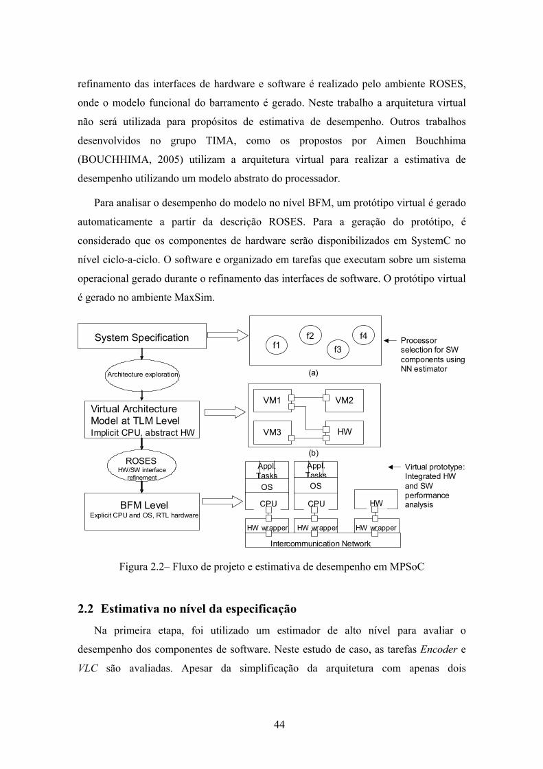
Para analisar o desempenho do modelo no nível BFM, um protótipo virtual é gerado

automaticamente a partir da descrição ROSES. Para a geração do protótipo, é

considerado que os componentes de hardware serão disponibilizados em SystemC no

nível ciclo-a-ciclo. O software e organizado em tarefas que executam sobre um sistema

operacional gerado durante o refinamento das interfaces de software. O protótipo virtual

é gerado no ambiente MaxSim.

Virtual ArchitectureModel at TLM LevelImplicit CPU, abstract HW

BFM LevelExplicit CPU and OS, RTL hardware

ROSESHW/SW interface

refinement

VM1 VM2

VM3 HW

Appl.Tasks

OS

HW wrapper

CPU HW

Intercommunication Network

CPU

HW wrapper HW wrapper

Appl.Tasks

OS



f1f2

f3f4 Processor

selection for SW components using NN estimator

Virtual prototype:Integrated HW and SW performance analysis

(a)

(b)

Figura 2.2– Fluxo de projeto e estimativa de desempenho em MPSoC

2.2 Estimativa no nível da especificação

Na primeira etapa, foi utilizado um estimador de alto nível para avaliar o

desempenho dos componentes de software. Neste estudo de caso, as tarefas Encoder e

VLC são avaliadas. Apesar da simplificação da arquitetura com apenas dois

45

processadores, a seleção do processador é um aspecto importante na exploração do

espaço de projeto.

Nos experimentos, dois processadores são utilizados: ARM946 e PowerPC750.

Estes processadores têm certas características como pipeline e memória cache que

tornam a estimativa de desempenho difícil.

A rede neural necessita de um conjunto de treinamento para calibrar o estimador.

Um conjunto de 41 benchmarks é utilizado para treinar e testar a precisão do estimador.

A Figura 2.3 apresenta a rede neural utilizada para estimar o desempenho do

processador ARM, onde as entradas são o número de instruções executadas pela

aplicação (classificadas por tipo).

InputLayer

HiddenLayer

OutputLayer

Forward Branches

Backward Branches

Load/Store

Multiple Load/Store

ALU

Cycles

Figura 2.3- Estimador para o processador ARM946

Para cada processador, um conjunto diferente de tipos de instrução é escolhido de tal

forma que estes representem da melhor forma o desempenho da aplicação. No caso do

processador PowerPC750, as instruções são classificadas como: desvio para um

endereço à frente, desvio para trás, load/store, operações em inteiros e operações de

ponto flutuante (Figura 2.4).

Para o treinamento da rede neural, um simulador ciclo-a-ciclo é necessário para

obter as instruções executadas e os ciclos consumidos. Para o processador ARM, o

simulador fornecido no ambiente MaxSim (ARM, 2007) é utilizado, e para o

processador PowerPC750 é utilizado o simulador Microlib (MICROLIB, 2007).

46

InputLayer

HiddenLayer

OutputLayer

Forward Branches

Backward Branches

Load/Store

Integer

Floats

Cycles

Figura 2.4- Estimador para o processador PowerPC750

A Tabela 2.1 resume os resultados obtidos pelo estimador baseado em redes neurais

para as arquiteturas ARM946 e PowerPC750. O custo principal da estimativa é

relacionado à obtenção do número de instruções executadas. Neste trabalho, as

instruções executadas são obtidas utilizando um simulador funcional disponível nos

ambientes MaxSim e Microlib para os processadores ARM946 e PowerPC750

respectivamente. O método proposto permite uma rápida estimativa comparado com a

simulação ciclo-a-ciclo devido à aceleração fornecida pelos simuladores funcionais.

Tabela 2.1- Ciclos estimados nos processadores ARM e PowerPC

ARM (ciclos) ARM (instruções) PowerPC (ciclos) PowerPC (instruções)

Encoder Task 255250 128230 114230 155032

VLC task 52694 23497 31478 25153

Os resultados da estimativa de desempenho são utilizados para auxiliar nas decisões

sobre a escolha do processador que executará a parte em software. Após a seleção do

processador, esta decisão é assinalada em cada componente de software na arquitetura

virtual no modelo ROSES. Esta informação será utilizada durante a geração das

interfaces de hardware e software que serão montadas a partir de uma biblioteca de

componentes. Em nosso estudo de caso, serão apresentados o refinamento e geração do

protótipo virtual utilizando processadores ARM946, e será comparado o desempenho

obtido com o protótipo virtual com os resultados obtidos com as redes neurais.

47

2.3 Estimativa de desempenho utilizando protótipos virtuais

Após a geração das interfaces de hardware e software é utilizado um protótipo

virtual para validar e analisar o desempenho do sistema no nível funcional do

barramento (BFM). O ambiente MaxSim(ARM, 2007) é utilizado para gerar o protótipo

virtual, permitindo a avaliação do desempenho. Os componentes em hardware são

considerados como blocos de propriedade intelectual (IP), disponibilizados em

SystemC. As interfaces em hardware geradas pelo ambiente ROSES durante o

refinamento também são disponíveis em SystemC. Os componentes SystemC são

encapsulados em componentes MaxSim, para que os componentes sejam disponíveis

para simulação. Os componentes de software juntamente com o sistema operacional são

compilados para a arquitetura alvo e carregados no simulador do processador durante a

inicialização da simulação.

A Figura 2.5 apresenta o protótipo virtual do codificador MPEG4 no ambiente

MaxSim. O protótipo virtual foi gerado automaticamente a partir da descrição ROSES.

A arquitetura é composta por dois subsistemas contendo processadores (VPROC0 e

VVLC0) que são responsáveis pela execução das tarefas Encoder e VLC. Os

componentes em hardware VINPUT, VCOMBINER e VDMA são descritos em

SystemC. Os componentes de simulação VANTENNA e VSTORAGE são utilizados

para enviar a imagem de entrada e para armazenar a imagem de saída.

A Figura 2.6 apresenta em detalhes o subsistema VPROC0. As interfaces de

hardware geradas pelo ambiente ROSES são automaticamente importadas no ambiente

MaxSim, como os decodificadores de endereço e o controlador de memória

(CMIMemCtrl). O componente CMIarm7cc implementa os adaptadores utilizados para

coordenar as transferências através do DMA.

48

Figura 2.5 – Protótipo virtual do codificador MPEG4 importada no ambiente MaxSim


Figura 2.6– Subsistema do componente VPROC0

49

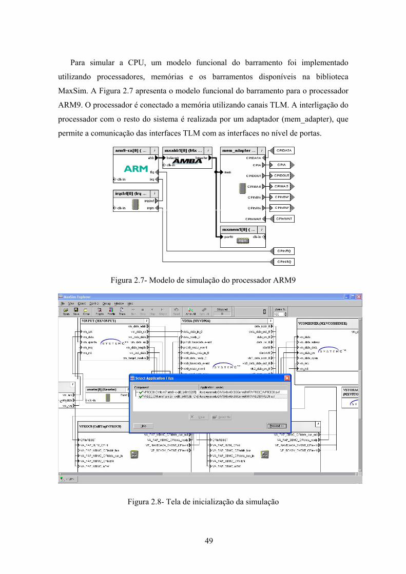
Para simular a CPU, um modelo funcional do barramento foi implementado

utilizando processadores, memórias e os barramentos disponíveis na biblioteca

MaxSim. A Figura 2.7 apresenta o modelo funcional do barramento para o processador

ARM9. O processador é conectado a memória utilizando canais TLM. A interligação do

processador com o resto do sistema é realizada por um adaptador (mem_adapter), que

permite a comunicação das interfaces TLM com as interfaces no nível de portas.

Figura 2.7- Modelo de simulação do processador ARM9

Figura 2.8- Tela de inicialização da simulação

50

O ambiente MaxSim Explorer é utilizado para simular o sistema. A Figura 2.8

apresenta a tela de inicialização da simulação. Durante a inicialização, os arquivos

contendo os binários da aplicação e do sistema operacional são carregados na memória.

O ambiente MaxSim fornece um suporte para a validação global, utilizando pontos

de parada (breakpoints) no código da aplicação, registradores, posições da memória e

conexões. A Figura 2.9 apresenta a tela com o código assembler da tarefa VLC. O

ambiente suporta o debug de todos os processadores simultaneamente, facilitando a

validação de aplicações concorrentes executando em arquiteturas MPSoC.

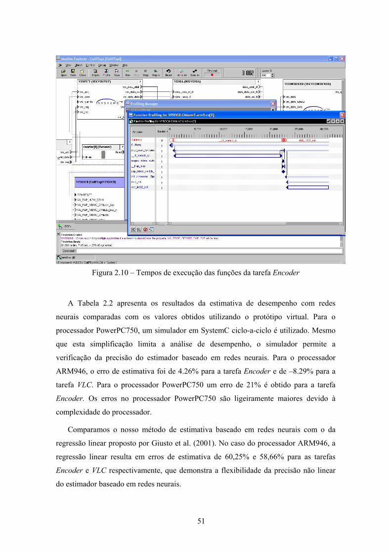
A Figura 2.10 apresenta os tempos de execução do software dividido por funções no

processador VPROC0 (tarefa Encoder). Este tipo de análise permite a detecção de

pontos de otimização e quais são as funções que gastam mais ciclos durante a execução

da aplicação.

Figura 2.9- Sessão de debug do código fonte da tarefa VLC

51

Figura 2.10 – Tempos de execução das funções da tarefa Encoder

A Tabela 2.2 apresenta os resultados da estimativa de desempenho com redes

neurais comparadas com os valores obtidos utilizando o protótipo virtual. Para o

processador PowerPC750, um simulador em SystemC ciclo-a-ciclo é utilizado. Mesmo

que esta simplificação limita a análise de desempenho, o simulador permite a

verificação da precisão do estimador baseado em redes neurais. Para o processador

ARM946, o erro de estimativa foi de 4.26% para a tarefa Encoder e de –8.29% para a

tarefa VLC. Para o processador PowerPC750 um erro de 21% é obtido para a tarefa

Encoder. Os erros no processador PowerPC750 são ligeiramente maiores devido à

complexidade do processador.

Comparamos o nosso método de estimativa baseado em redes neurais com o da

regressão linear proposto por Giusto et al. (2001). No caso do processador ARM946, a

regressão linear resulta em erros de estimativa de 60,25% e 58,66% para as tarefas

Encoder e VLC respectivamente, que demonstra a flexibilidade da precisão não linear

do estimador baseado em redes neurais.

52

Tabela 2.2- Comparação entre a estimativa baseado em redes neurais e o protótipo

virtual

ARM946 PowerPC750

Estimado Ciclo-a-ciclo Erro Estimado Ciclo-a-ciclo Erro

Encoder

Task 255250 266630 4.26% 114230 151960 24.8%

VLC Task 52694 48659 -8.29% 31478 31064 1.33%

A Tabela 2.3 apresenta os tempos necessários (em segundos) para a estimativa e a

execução do protótipo virtual. A estimativa baseada em redes neurais permite uma

aceleração considerável comparado com a simulação utilizando protótipos virtuais. As

redes neurais permitem uma rápida estimativa de desempenho. Tal característica é

importante devido ao aumento da parte em software nos sistemas embarcados. Por outro

lado, o protótipo virtual fornece uma solução global de análise integrada dos

componentes de hardware e software que permite a confirmação dos valores obtidos na

estimativa de alto nível.

Tabela 2.3 – Tempos de simulação do protótipo virtual comparados com a estimativa

baseada em redes neurais

ARM946 PowerPC750

Ciclo-a-

ciclo(s)

Estimativa

(s)

Aceleração Ciclo-a-

ciclo (s)

Estimativa

(s)

Aceleração

Encoder Task 5.5 0.3 22.0 4.3 0.3 14.3

VLC Task 3.0 0.2 14.3 1.4 0.2 6.5

53

3 CONCLUSÃO

Nesta tese, é proposta uma metodologia integrada para a concepção e estimativa de

desempenho em sistemas multiprocessados em único chip (MPSoC), onde o suporte

para a estimativa de desempenho é fornecido durante o fluxo de projeto. O ambiente

ROSES desenvolvido no grupo TIMA é utilizado como fluxo de projeto e foi integrado

com as ferramentas de estimativa de desempenho desenvolvidas nesta tese.

No nível da especificação, é proposta a utilização de estimadores analíticos para

guiar a seleção do processador, permitindo uma estimativa rápida e precisa. As redes

neurais são utilizadas como estimadores devido à flexibilidade e adaptação não-linear

necessária para a estimativa de desempenho em processadores complexos. Os resultados

da utilização das redes neurais como estimadores foram apresentados em um artigo

(OYAMADA et al., 2004), na conferência SBCCI.

Métodos baseados em simulação são utilizados para analisar o desempenho do

sistema no nível funcional do barramento (BFM). Neste trabalho, duas ferramentas

(FlexPerf e MaxSim) são integradas no fluxo de projeto ROSES.

A primeira ferramenta chamada FlexPerf, foi desenvolvida para a análise de

desempenho do software embarcado. Esta ferramenta foi integrada ao fluxo de projeto

ROSES possibilitando a análise de desempenho de arquiteturas geradas pelo ROSES.

Na integração, os modelos de simulação de processador com suporte à análise de

desempenho fornecidos pelo FlexPerf foram integrados ao modelo de simulação

SystemC gerado pelo ambiente ROSES. Esta integração adicionou ao ROSES todo o

suporte a instrumentação e análise de desempenho fornecidas pelo ambiente FlexPerf.

A segunda ferramenta integrada ao ambiente ROSES foi a ferramenta para

modelagem e simulação de protótipos virtuais MaxSim. Para criar um protótipo virtual,

54

uma ferramenta foi implementada para que o modelo ROSES no nível BFM seja gerado

automaticamente no ambiente MaxSim. Para a execução da parte em software os

simuladores ciclo-a-ciclo disponíveis no MaxSim são utilizados. O protótipo virtual

fornece um modelo de validação global, permitindo o debug de aplicações concorrentes

executando em arquiteturas MPSoC.

Para validar as ferramentas de estimativa de desempenho desenvolvidas nesta tese

um estudo de caso de um codificador MPEG4 baseado em uma arquitetura

multiprocessada foi demonstrado. Esta plataforma apresenta alguns desafios para a

análise de desempenho tais como a existência de múltiplos processadores e de

componentes de propriedade intelectual. O estudo de caso permitiu a avaliação da

estimativa de desempenho em alto nível e a comparação com os resultados obtidos na

simulação ciclo-a-ciclo utilizando o protótipo virtual. Este trabalho foi apresentado na

conferência ASPDAC (OYAMADA et al., 2007).

3.1 Limitação dos métodos propostos e trabalhos futuros

A partir dos resultados obtidos no desenvolvimento dos estudos de caso, algumas

limitações podem ser identificadas:

a) A precisão da rede neural é dependente da qualidade das entradas

utilizadas durante a fase de treinamento. Neste trabalho, um conjunto

de treinamento foi selecionado para favorecer a generalização,

utilizando aplicações de diferentes tamanhos e domínios;

b) Para o treinamento um estimador ciclo-a-ciclo é necessário. Para a

etapa de utilização, a fim de obter as instruções executadas um

simulador funcional é utilizado. A aceleração do método proposto

neste trabalho é dependente da aceleração fornecida pelo simulador

funcional em relação ao simulador ciclo-a-ciclo;

c) O protótipo virtual utiliza a simulação que tem um custo elevado para

a execução de grandes arquiteturas com vários processadores. Neste

caso, o protótipo virtual poderá ser utilizado para analisar somente

partes específicas do software como a inicialização ou o tratamento de

interrupções.

55

Apesar das contribuições obtidas neste trabalho, algumas perspectivas potenciais

podem ser identificadas:

a) O estudo da aplicação de redes neurais para a estimativa da energia

consumida pelo software;

b) A utilização dos parâmetros arquiteturais na rede neural, como

proposto por Ipek et al. (2006);

c) A utilização de uma ferramenta de profile genérica e a posterior

tradução para o processador alvo, com o objetivo de substituir o

simulador funcional utilizado na etapa de utilização da rede neural;

d) A integração dos métodos de estimativa propostos neste trabalho com

outras linguagens de alto nível como UML e Simulink;

e) A geração do protótipo virtual utilizando canais TLM, fornecendo

assim uma simulação mais rápida.

57

ANNEXE B SOFTWARE PERFORMANCE ESTIMATION IN MPSoC DESIGN

Marcio Seiji OYAMADA Laboratoire TIMA – INPG

LSE Lab - UFRGS

59

CONTENTS

LIST OF ABBREVIATIONS AND ACRONYMS .............................................. 61

LIST OF FIGURES........................................................................................... 63

LIST OF TABLES ............................................................................................ 67

ABSTRACT...................................................................................................... 69

RESUMO.................................................. ERRO! INDICADOR NÃO DEFINIDO.

1 INTRODUCTION....................................................................................... 71

1.1 Performance Estimation in MPSoC Design ................................................... 72 1.2 Need for Improvement ..................................................................................... 74 1.3 Integration in MPSoC Design Flow ................................................................ 74

2 MPSOC DESIGN ...................................................................................... 78

2.1 Design Methodologies....................................................................................... 79 2.1.1 Abstraction Levels.......................................................................................... 79 2.1.2 Platform-based Design ................................................................................... 80 2.1.3 Component-based Design............................................................................... 80 2.2 MPSoC Architectures ...................................................................................... 81 2.2.1 Processor......................................................................................................... 81 2.2.2 Memory .......................................................................................................... 83 2.2.3 Interconnection ............................................................................................... 84 2.2.4 SoC Platforms................................................................................................. 85 2.3 Software Design ................................................................................................ 87 2.3.1 Programming Models ..................................................................................... 88 2.4 ROSES MPSoC Design Environment ............................................................ 91 2.4.1 HW/SW Interface Abstraction ....................................................................... 92 2.4.2 HW Wrapper Generation - ASAG.................................................................. 94 2.4.3 SW Wrapper Generation – ASOG ................................................................. 94 2.4.4 Simulation Model Generation – CosimX ....................................................... 95 2.5 Performance Estimation .................................................................................. 96 2.5.1 Software Performance Estimation.................................................................. 97 2.5.2 Integrated Hardware and Software Performance Estimation ....................... 101 2.6 Integrated MPSoC design and software performance estimation ............. 109 2.6.1 Discussion..................................................................................................... 112

3 ANALYTIC SOFTWARE PERFORMANCE ESTIMATION..................... 114

60

3.1 Neural Network Performance Estimation.................................................... 115 3.2 Experimental Set ............................................................................................ 119 3.3 Generic Estimator .......................................................................................... 120 3.3.1 PowerPC Generic Estimator......................................................................... 120 3.3.2 FemtoJava- a Java Microcontroller .............................................................. 123 3.3.3 Athlon XP Generic Estimator....................................................................... 124 3.4 Automatic Domain Classification ................................................................. 125 3.4.1 PowerPC 750 Domain-specific Estimator.................................................... 126 3.4.2 Athlon XP Domain-specific Estimator......................................................... 127 3.5 Conclusions ..................................................................................................... 128

4 PERFORMANCE ESTIMATION AND ANALYSIS USING AN INTEGRATED HARDWARE AND SOFTWARE SIMULATION MODEL....... 130

4.1 FlexPerf ........................................................................................................... 133 4.1.1 System Architecture View............................................................................ 135 4.1.2 Application View.......................................................................................... 135 4.1.3 Analysis View .............................................................................................. 135 4.1.4 Simulator Instrumentation ............................................................................ 136 4.2 ROSES and FlexPerf Integration.................................................................. 137 4.2.1 Case Study- FIFO Analysis in a Monoprocessor System............................. 139 4.2.2 Case Study- MPEG4 Encoder Multiprocessor System ................................ 140 4.3 MaxSim ESL Design....................................................................................... 143 4.4 ROSES Integration......................................................................................... 145 4.5 Conclusions ..................................................................................................... 146

5 CASE STUDY ......................................................................................... 148

5.1 Performance Estimation and Analysis Flow................................................ 149 5.2 High-level Estimation..................................................................................... 150 5.3 Virtual Prototype Performance Analysis ..................................................... 152 5.3.1 MPEG4 Encoder Virtual Prototype.............................................................. 153

6 DISCUSSION AND FINAL REMARKS................................................... 160

6.1 Limitations of the Proposed Methods and Future Works .......................... 161

REFERENCES............................................................................................... 163

61

LIST OF ABBREVIATIONS AND ACRONYMS

ADL Architecture Description Language API Application Programming Interface ASIC Application-Specific Circuit BFM Bus-Functional Model CFG Control Flow Graph CISC Complex Instruction Set Computer CMOS Complementary metal-oxide semiconductor CPU Central Processing Unit CPI Cycles per instruction DMA Direct Memory Access DSP Digital Signal Processor FIFO First-In First-Out GPP General Purpose Processor GUI Graphical User Interface HAL Hardware Abstraction Layer HW Hardware I/O Input and Output IP Intellectual Property IPC Inter-Process Communication ISS Instruction Set Simulator MIMD Multiple Instruction Multiple Data MPEG Moving Picture Experts Group MPSoC Multiprocessor System-on-Chip OS Operating System PDA Personal Digital Assistant RISC Reduced Instruction Set Computer RTL Register-transfer Level RTOS Real-time Operating System SIMD Single Instruction Multiple Data SMP Symmetric Multiprocessing SoC System-on-chip SW Software TLM Transaction-Level Model UML Unified Modeling Language VLC Variable Length Coding VLIW Very Long Instruction Word WCET Worst-Case Execution Time XML Extended Markup Language

63

LIST OF FIGURES

Figure 1.1- Typical MPSoC solution.............................................................................. 71

Figure 1.2- Concurrent HW/SW codesign (JERRAYA, 2005)...................................... 72

Figure 1.3- Performance estimation tools and abstraction levels................................... 73

Figure 1.4- Performance estimation design flow ........................................................... 75

Figure 2.1- MPSoC abstraction levels............................................................................ 79

Figure 2.2- Market share of 32-bit embedded processors (IDC, 2007).......................... 81

Figure 2.3- Operational states in StrongARM processor (BENINI, 2000) .................... 82

Figure 2.4- Processor power-consumption (ZHANG; VAHID; LYSECKY, 2004)...... 83

Figure 2.5- Cache size and its influence on system power consumption (ZHANG; VAHID; LYSECKY, 2004) ................................................................................... 84

Figure 2.6- Communication topologies (a) point-to-point, (b) bus-based connection, and (c) network-on-chip ................................................................................................ 85

Figure 2.7- Nomadik architecture (NOMADIK, 2007).................................................. 85

Figure 2.8- Platform OMAP 1610 (OMAP, 2007)......................................................... 86

Figure 2.9- Phillips Nexperia PNX8550 (GOOSSENS et al., 2005) ............................. 87

Figure 2.10- Software application layers........................................................................ 88

Figure 2.11- OpenMP parallel program example........................................................... 89

Figure 2.12- Distributed objects components................................................................. 90

Figure 2.13- DSOC model for platform mapping (PAULIN et al., 2004) ..................... 91

Figure 2.14- ROSES design flow (CESARIO et al., 2002)............................................ 92

Figure 2.15- Virtual architecture (CESARIO et al., 2002)............................................. 93

Figure 2.16- Hardware wrapper architecture (CESARIO et al., 2002) .......................... 94

Figure 2.17- Application-specific OS generation flow (GAUTHIER et al., 2001)........ 95

Figure 2.18- Executable model generation in CosimX (SARMENTO et al., 2004)...... 96

Figure 2.19- Static WCET analysis ................................................................................ 98

Figure 2.20- MPARM system architecture example (BENINI et al., 2005) ................ 102

Figure 2.21- LISA simulation and SystemC integration levels (WIEFERINK et al., 2004)..................................................................................................................... 103

64

Figure 2.22- Adaptation between event models in SymTA/S (RITCHER et al., 2003).............................................................................................................................. 105

Figure 2.23- Lahiri’s method for communication architecture exploration (LAHIRI et al., 2001) ............................................................................................................... 107

Figure 2.24- Platune SoC base platform (GIVARGIS; VAHID, 2001)....................... 108

Figure 2.25- Integrated MPSoC design and performance estimation flow .................. 110

Figure 3.1- Performance estimation tool in a global design flow ................................ 115

Figure 3.2- Estimation tool development and utilization ............................................. 117

Figure 3.3- Steps in the training phase of the estimator ............................................... 117

Figure 3.4- Estimator utilization phase ........................................................................ 118

Figure 3.5- The neural network and the transfer functions used in its hidden layer and output layer ........................................................................................................... 118

Figure 3.6- Cycle and instruction count distribution.................................................... 120

Figure 3.7- NN for the PowerPC experiments ............................................................. 121

Figure 3.8- Prediction errors using 5 input parameters: backward branch, forward branch, load/store, integer, and floating-point...................................................... 122

Figure 3.9- Prediction errors for the FemtoJava microcontroller................................. 123

Figure 3.10- CFG weight method................................................................................. 125

Figure 3.11- Estimation process with automatic domain classification ...................... 126

Figure 3.12- Comparison between generic and domain-specific estimators for 3 different architectures (Athlon XP, PowerPC, and ADSP) .................................. 128

Figure 4.1- Performance estimation tools in MPSoC design ....................................... 130

Figure 4.2- SoC design flow......................................................................................... 131

Figure 4.3- Performance estimation using CPU abstract models (adapted from Bouchhima (2005))............................................................................................... 132

Figure 4.4- FlexPerf graphical user interface (PAOLI; SANTANA; GALIX, 2004).. 134

Figure 4.5- FlexPerf framework components............................................................... 134

Figure 4.6- Simulator instrumentation from LISA processor description.................... 136

Figure 4.7- FIFO channel instrumentation example..................................................... 137

Figure 4.8- ROSES and FlexPerf integration flow....................................................... 138

Figure 4.9- FIFO simulation model.............................................................................. 139

Figure 4.10- FIFO analysis results ............................................................................... 140

Figure 4.11- MPEG4 encoder architecture (BONACIU et al., 2006) .......................... 141

Figure 4.12- MPEG4 encoder top-level architecture.................................................... 141

Figure 4.13- CPU subsystem for the VPROC0 component ......................................... 142

Figure 4.14- DMA transfer analysis at BFM Level ..................................................... 143

65

Figure 4.15- MaxSim component interfaces (ARM, 2007) ......................................... 144

Figure 4.16- MaxSim model example .......................................................................... 144

Figure 4.17- MaxSim SystemC wrapper ...................................................................... 145

Figure 4.18- SystemC encapsulation in MaxSim components..................................... 145

Figure 4.19- MaxSim integration in the ROSES design flow ...................................... 146

Figure 5.1- MPEG4 encoder architecture (Bonaciu et al., 2006) ................................. 148

Figure 5.2- MPEG4 architecture with four Encoder tasks and two VLC tasks ............ 149

Figure 5.3- MPSoC performance estimation design flow ............................................ 150

Figure 5.4- NN performance estimation for the ARM9 processor............................... 151

Figure 5.5- NN performance estimation for the PowerPC750 processor..................... 151

Figure 5.6- Top-level model of the MPEG4 encoder................................................... 154

Figure 5.7- CPU subsystem for the VPROC0 component ........................................... 154

Figure 5.8- BFM model of the ARM9 processor in MaxSim ...................................... 155

Figure 5.9- MaxSim Explorer initial screen ................................................................. 155

Figure 5.10- Software debugging support in MaxSim ................................................. 156

Figure 5.11- Software timeline execution .................................................................... 157

Figure 5.12- Bus transfer analysis ................................................................................ 158

Figure 5.13- DMA transfer analysis ............................................................................. 158

67

LIST OF TABLES

Table 4.1- Comparison between the cycle-accurate simulation and the proposed estimation method ................................................................................................ 116

Table 4.2- Benchmarks used in experiments................................................................ 119

Table 4.3- Estimation results for the 41-benchmark set............................................... 121

Table 4.4- Estimation performance using the LOO (leave-one-out) training technique.............................................................................................................................. 123

Table 4.5- Estimation speed-up for the FemtoJava processor ..................................... 124

Table 4.6- Results with a generic estimator for the Athlon XP.................................... 124

Table 4.7- Estimation results using domain-specific estimators .................................. 127

Table 4.8- Estimation results using domain-specific estimators for an AthlonXP processor............................................................................................................... 127

Table 6.1- Estimation and instruction count for the ARM and PowerPC processors .. 152

Table 6.2- High-level performance estimation (in cycles) compared to the cycle-accurate virtual prototype ..................................................................................... 159

Table 6.3- Estimation and cycle-accurate virtual prototype simulation times ............. 159

69

ABSTRACT

Nowadays, embedded system complexity requires new design methodologies. System-level methodologies are proposed to cope with this complexity, starting the design above the register-transfer level. Performance estimation tools are an important piece of system-level design methodologies, since they are used to aid design space exploration at an early design stage. The goal of this thesis is to define an integrated methodology for software performance estimation. Currently, embedded software usage is increasing, becoming multiprocessor system-on-chip a common solution to cope with flexibility, performance, and power requirements. The development of accurate software performance estimators is not trivial, due to the increased complexity of embedded processors. To drive processor selection at specification level, a novel analytic software performance estimator based on neural networks is proposed. The neural network enables a fast estimation at an early design stage. To target the software performance analysis at bus functional level, where mapping of the hardware and software components is already established, we use a global simulation model supporting performance profiling. The proposed software performance estimation methodology is linked to a hardware and software interface refinement environment named ROSES. The proposed methodology is evaluated through a case study of a multiprocessor MPEG4 encoder.

Keywords: Performance estimation, MPSoC design, design space exploration

1 INTRODUCTION

Increases in chip integration capacity and transistor number have allowed the development of solutions called System-on-Chip (SoC). An SoC solution integrates processors, application specific HW components, digital interfaces and, occasionally, analog interfaces.

The convergence of various products, such as cellular phones with music players and PDAs with digital video capabilities makes these products more and more heterogeneous and requires high performance.

Nowadays embedded systems are characterized by real-time requirements, power and energy constraints, as well as cost and time-to-market pressure. Multimedia functionalities impose real-time constraints in order to correctly execute behavior. Mobile devices powered by batteries require low-power and low-energy capabilities. On the one hand, time-to-market pressure calls for fast design but, on the other hand, such products are cost sensitive, thus requiring an optimized design.

Flexibility is another important requirement. The design must be flexible enough to allow for new functionalities without needing to redesign. Microprocessors play an important role in providing the flexibility and heterogeneity needed in new embedded systems. Nowadays, SoC solutions with one or more processors are becoming more and more common. These solutions, called multiprocessor-on-chip (MPSoC), require new tools and programming models to cope with their complexity (JERRAYA, 2005).

Figure 1.1 shows a typical MPSoC architecture composed of two processors and application-specific HW components. An intercommunication network connects the MPSoC components. A wrapper may be necessary to adapt the components’ interface to the intercommunication network. Usually, the application software is divided in tasks and a real-time operating system provides execution and communication support through an application programming interface (API).

Appl.Tasks

OS

HW wrapper

CPU HW


CPU


Appl.Tasks

OS

Figure 1.1- Typical MPSoC solution

72

MPSoC designs have to consider HW and SW components in an integrated way. Currently, the hardware and software integration is done after a hardware prototype is available. As a consequence, integration problems will be detected in a late design stage resulting in unacceptable delays.

System-level design methodologies enable concurrent hardware and software design as presented in Figure 1.2. The key idea is to use a specification that models the hardware and software in a unified representation. The architecture exploration step uses the specification to partition the functionalities among hardware and software components. Architecture exploration results in a virtual architecture composed of functional hardware and software modules. Usually, transaction-level channels interconnect the components providing abstract HW/SW interfaces. From this virtual architecture, the traditional hardware and software development flow is followed with the refinement of the abstract hardware and software interfaces. Abstract interface refinement comprises mapping the communication API to a real-time operating system and building HW adapters. Subsequently, the design flow resumes with the physical hardware design and the software design.

System specification

Embedded software design

HW-SW codesign- CPU subsystem design- HW dependent SW design- SW dependent HW design

Back-end and hardware prototypes

Hardware modules design


Abstract HW-SW interface model- API for SW modules- abstract interfaces for HW modules- QoS specification

SW module specification

HW module specification

Embedded system

System specification

Embedded software design

HW-SW codesign- CPU subsystem design- HW dependent SW design- SW dependent HW design

Back-end and hardware prototypes

Hardware modules design


Abstract HW-SW interface model- API for SW modules- abstract interfaces for HW modules- QoS specification

SW module specification

HW module specification

Embedded system

Figure 1.2- Concurrent HW/SW codesign (JERRAYA, 2005)

1.1 Performance Estimation in MPSoC Design

In order to obtain an optimized design, the MPSoC design flow needs estimation tools to drive architecture exploration and to verify if the design fulfills requirements. Performance is

73

normally the main criterion adopted to guide architecture exploration. However, other aspects, such as power, energy and area, need to be considered as early as possible in the design flow.

Fast design space exploration strategies need to be developed in order to explore design alternatives at system-level. This requires high-level performance estimation tools integrated with exploration strategies in order to help the designer rank design alternatives.

Performance estimation is a continuous process and can be applied at different abstraction levels throughout the design flow, as shown in Figure 1.3. At specification level, this includes HW/SW partitioning, processor selection, and assignment of tasks to processors. The interconnection structure can be explored at the virtual architecture level. At the bus-functional level, the architecture is almost defined and includes the HW/SW interfaces as well as the software compiled for the target architecture. At this level, cycle-accurate models allows for precise evaluation of system performance.


BFM Level

SoC Integration

RTL Level





Processor Selection


Memory mapping

Delay estimation

Scope of this work

Figure 1.3- Performance estimation tools and abstraction levels

Due to the growing number of processors in MPSoC designs and, consequently, the increasing relevance of the software portion, high-level software performance estimation tools are needed. Monoprocessor software estimation tools can be divided in three groups: simulations, abstract models and hybrid methods (MEYEROWITZ, 2004). Simulation-based methods use cycle-accurate simulators to estimate software execution time, whereas analytic methods use abstract models and cost functions. Hybrid methods use code annotation (at instruction or basic block level) with execution cost. The application runs natively, thus avoiding the long simulation time of cycle-accurate simulators.

For the MPSoC architecture, an integrated estimation method must consider the hardware and software components and the contribution of each individual component in the whole system performance. It requires integrated hardware and software estimation tools, which can

74

be classified as simulation, trace-based, or analytical-based methods. Simulation-based methods use instruction set simulators for the software part and hardware simulation models in order to obtain a system-level simulation model. Trace-based methods record access to system resources (for example, computation and communication elements) produced by a generic system simulation. An architecture is evaluated by mapping the trace onto the architecture resources. This idea is well known and applied in cache performance evaluation, where a trace of memory access is mapped and performance is evaluated for a given cache architecture and policy. Analytical methods are proposed to provide fast performance estimation and avoid exhaustive simulation, which is prohibitive. Usually, the system is modeled as a set of properties (for example, event rate and instruction usage), and abstract models calculate system performance based on these properties. Analytical methods are less accurate than simulation or trace-based methods, but they can quickly identify interesting solutions, which will later be subjected to a more detailed analysis.

1.2 Need for Improvement

This work deals with software performance estimation. Performance estimation tools are needed due to the large design space that cannot be manually explored or verified when only a hardware prototype is available. Advanced processor architectures and complex applications make simulation prohibitive for high-level performance estimation. Analytical methods have been proposed using databook or linear models that fail to precisely estimate the performance in advanced architectures. This work proposes a neural network-based software performance estimator. The estimator generates a fast estimation from descriptions in C code and is developed to be applied in high-level architecture exploration.

An integrated hardware and software estimation tool is necessary, also, due to complex interaction and synchronization scenarios. Virtual prototypes can deal with this problem providing a single model to evaluate hardware and software performance after architecture exploration. In a virtual prototype, software is executed using a simulation model of the target processor and the hardware using functional models. This permits the generation of a global simulation model, where the hardware and software are simulated in a synchronized way. In this work, a virtual prototype environment is integrated to an MPSoC design environment, providing automatic generation model, which facilitates the design evaluation of complex MPSoCs.

1.3 Integration in MPSoC Design Flow

The main objective of this thesis is to provide a methodology for software performance estimation integrated in an MPSoC design flow. In this work, the ROSES design environment is used as a design flow to guide performance estimation. ROSES uses a component-based approach to refine the hardware and software interfaces in an MPSoC design. As input, it uses a virtual architecture composed of hardware and software modules interconnected by transaction-level model (TLM) channels. ROSES assumes that external tools are utilized to make the partitioning between hardware and software components at the functional level. Hardware components are considered black-box components. Software components are divided in tasks. To drive hardware and software interface refinement, each software module is mapped to a given processor.

In this work, we propose a new high-level software estimation method based on neural networks (NN) to guide processor selection, as shown in Figure 1.4(a). In our experiments,

75

neural networks provided suitable accuracy and flexibility for software performance estimation, even in complex architectures. These experiments were carried out using five different architectures: PowerPC 750, AthlonXP, ARM946, ADSP, and a Java processor called FemtoJava.




refinement

VM1 VM2

VM3 HW

Appl.Tasks

OS

HW wrapper

CPU HW


CPU


Appl.Tasks

OS



f1f2

f3f4 Processor



(a)

(b)

(c)

Figure 1.4- Performance estimation design flow

ROSES (CESARIO et al., 2002) refines the virtual architecture and generates a bus functional model (BFM), as shown in Figure 1.4(c). This bus functional model is composed of processors that execute the software and by hardware wrappers necessary to interconnect the hardware components. Software tasks execute under an application-specific operating system that implements the application programming interface (API) used in communication and synchronization between hardware and software components.

The virtual architecture differs from the BFM model in terms of the components interface and the software. In the virtual architecture the interfaces are modeled as transaction-level channels, whereas in the BFM model the interfaces are refined to pin-level interfaces. The ROSES environment provides a tool called CosimX, which generates a SystemC simulation model for the virtual architecture and the BFM model. In the virtual architecture, software is compiled for the host machine, and only the functional behavior and communication is validated. On the other hand, in the BFM model, the software is compiled for the target architecture and validated using a processor simulator. At this level, the whole architecture, including the operating system and hardware wrappers generated during the interfaces refinement step are validated.

In this work, we propose the generation of global simulation models using the BFM model to allow an integrated hardware and software performance analysis. This way, an automatic method to generate simulation models with performance analysis support is proposed, reducing design time and making performance analysis easier. These global simulation models, called virtual prototypes, are generated using two tools: FlexPerf(PAOLI; SANTANA; GALIX, 2004) and MaxSim(ARM, 2007).

76

The SystemC simulation model at BFM level, generated by CosimX, uses an instruction-accurate simulator for the software execution and SystemC modules for the hardware components. However, in this model the instruction-accurate simulator (software part) synchronizes with the hardware modules only when a communication occurs between them. The performance estimation capabilities provided by the SystemC model are limited and include the tracing of signals and the debug of the assembler code. The integration of a virtual prototype to the ROSES environment extends the performance analysis capabilities for the BFM model. The virtual prototype generated in this work provides a global model with the software and hardware components synchronized cycle-by-cycle. The virtual prototype enables performance analysis resources like software execution timeline and communication tracing. Moreover, the virtual prototype provides the debug of concurrent software executing in MPSoC architectures, allowing breakpoints at signals, assembler code, and registers.

The FlexPerf framework has a well-defined flow to generate a processor simulator using the LISA language, with all the necessary instrumentation support for performance analysis of embedded software. This method was used to integrate this stand-alone processor simulator in a global MPSoC simulation. A SystemC simulation model is generated to support the instrumentation using the FlexPerf framework. In this work, a multiprocessor MPEG4 encoder platform was implemented, allowing an integrated performance analysis of software and hardware components.

We also evaluate a virtual prototype environment called MaxSim. MaxSim provides a rich library of processors, memories, buses, and peripherals. Some components provide built-in performance analysis capabilities, such as cache performance and bus utilization. MaxSim supports custom SystemC modules, thus making integration with the ROSES environment easier. This integration is accomplished by automatically generating a MaxSim design from the ROSES architecture description. The same MPEG4 encoder platform used in the FlexPerf evaluation was simulated in the MaxSim evaluation. We mainly explored MaxSim’s performance analysis support functionality in the context of processor performance evaluation. The MaxSim profile interface was used to implement a custom performance analysis. In the case study (exposed in Chapter 6), an analysis of transfers handled by a DMA (direct memory access) IP component was implemented.

Usually, MPSoC simulation environments provide fixed capabilities for performance analysis. The FlexPerf framework provides a more flexible approach, integrating custom performance analysis. Although the instrumentation is developed manually, the possibility of extending and reusing analysis modules does save time. Integration with ROSES enables consistent performance analysis and design, which is not normally supported by other simulation tools. Further, the integration between an analytical estimation method at the specification level and a simulation-based approach at the virtual architecture and BFM levels provides a good compromise between estimation speed and accuracy.

For the virtual architecture level (Figure 1.4(b)), performance estimation is covered by other works developed in the TIMA laboratory. Bouchimma et al. (2005) propose an estimation method based on an abstract CPU model, in order to estimate software performance. The abstract CPU model executes the software natively but also represents resources like IO access and conflicts, providing a rapid, global validation. The virtual architecture model will not be directly used in this work.

This thesis is organized as follows. Chapter 2 presents general concepts relating to MPSoCs. Chapter 3 describes our proposed integrated MPSoC design and performance analysis flow. Chapter 4 presents a software performance estimator based on neural networks. Chapter 5 exposes two MPSoC integrated hardware and software estimation solutions based

77

on simulation. Chapter 6 describes a case study of the MPEG4 encoder architecture using the estimation tools developed in this work. Chapter 7 presents final remarks and conclusions.

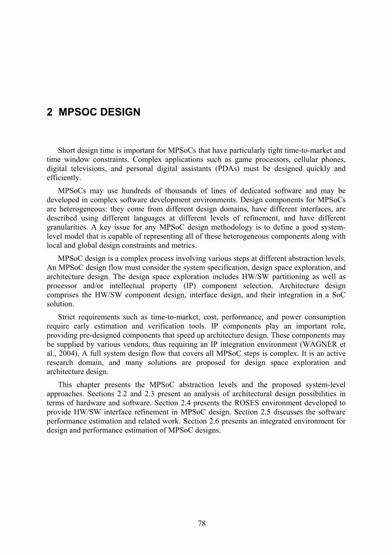
78

2 MPSOC DESIGN

Short design time is important for MPSoCs that have particularly tight time-to-market and time window constraints. Complex applications such as game processors, cellular phones, digital televisions, and personal digital assistants (PDAs) must be designed quickly and efficiently.

MPSoCs may use hundreds of thousands of lines of dedicated software and may be developed in complex software development environments. Design components for MPSoCs are heterogeneous: they come from different design domains, have different interfaces, are described using different languages at different levels of refinement, and have different granularities. A key issue for any MPSoC design methodology is to define a good system-level model that is capable of representing all of these heterogeneous components along with local and global design constraints and metrics.

MPSoC design is a complex process involving various steps at different abstraction levels. An MPSoC design flow must consider the system specification, design space exploration, and architecture design. The design space exploration includes HW/SW partitioning as well as processor and/or intellectual property (IP) component selection. Architecture design comprises the HW/SW component design, interface design, and their integration in a SoC solution.

Strict requirements such as time-to-market, cost, performance, and power consumption require early estimation and verification tools. IP components play an important role, providing pre-designed components that speed up architecture design. These components may be supplied by various vendors, thus requiring an IP integration environment (WAGNER et al., 2004). A full system design flow that covers all MPSoC steps is complex. It is an active research domain, and many solutions are proposed for design space exploration and architecture design.

This chapter presents the MPSoC abstraction levels and the proposed system-level approaches. Sections 2.2 and 2.3 present an analysis of architectural design possibilities in terms of hardware and software. Section 2.4 presents the ROSES environment developed to provide HW/SW interface refinement in MPSoC design. Section 2.5 discusses the software performance estimation and related work. Section 2.6 presents an integrated environment for design and performance estimation of MPSoC designs.

79

2.1 Design Methodologies

2.1.1 Abstraction Levels Abstract descriptions provide a suitable way to manage design complexity, hiding

implementation details that the designer may want to leave out at some point. In consequence, the description is short, making its understanding easier.

The design flow must define different abstraction levels and refinement steps that lead to a final solution (EDWARDS et al., 1997). Ideally, the designer would have the benefit of automatic refinement from higher abstraction levels to system implementation. As mentioned, MPSoC design is quite complex and the available tools do not cover all design steps.

Figure 2.1 shows abstraction levels usually applied to MPSoC design. The system specification describes the behavior of the system under development. Software engineers see the system specification as a document that describes the required functionalities, using abstract representations. For instance, using the UML notation, a system may be represented by class and use cases diagrams. Usually, in electronic design, an executable specification is used to represent system functionalities. Some languages have been proposed for electronic system specification, such as SystemC (2005) and SpecC (2007). These languages are extensions of existing imperative languages (for example, C++) and support hardware-oriented descriptions. However, the research community is now focusing on the use of more abstract specification languages such as UML and Simulink.




refinement

SoC Integration

RTL LevelExplicit SW memory mapping

VM1 VM2

VM3 HW

Appl.Tasks

OS

HW wrapper

CPU HW


CPUBFM


Appl.Tasks

OS

HW

Physical Network

CPU

MEM0MEM1

CPU

MEM0MEM1



f1f2

f3f4

HW wrapper

Figure 2.1- MPSoC abstraction levels

80

Architecture exploration uses the specification to define the golden architecture that covers application requirements in terms of performance, power consumption, energy consumption, and area, among others. From the architecture exploration step, a virtual architecture that represents the system in terms of software and hardware components is obtained. Transaction-level channels abstract the HW/SW interfaces, making possible the development of the software using –an application-programming interface (API). Functional HW components are used at this level, providing high simulation speed.

The virtual architecture is refined to a bus-functional level model, where the HW and SW interfaces are nearing final implementation. In the software interface refinement, an operating system, which includes a hardware abstraction layer (HAL) and low-level drivers, provides the API used by the application software. Communication protocols may require hardware components such as co-processors and channel adapters, which are responsible for adapting the internal component bus to the interconnection network.

The BFM level hides certain details of the final MPSoC RT-level. For example, ISS (instruction set simulators) at BFM-level do not use memory mapping and do not consider low-level initialization code, such that for caches and fast memory configuration. The SoC integration step includes such considerations and the resulting RTL model is used in the physical design (PETKOV et al., 2006).

2.1.2 Platform-based Design Platform-based design (KEUTZER et al., 2000) uses architecture templates to obtain a

solution called a derivative, by tailoring the platform for a given application. Architecture templates are domain-specific hardware platforms composed of processors, memories, hardware blocks, and communication structures. Occasionally, these components have some degree of configurability, such as processor caches and memory sizes.

Software is becoming the most important part of MPSoC platforms. An application-programming interface (API) provides the means to abstract the communication between components. An operating system (OS) implements services such as task scheduling and inter-process communication. It also improves the reusability of software IP components because it builds an abstraction layer that makes application software portable to different hardware platforms.

Platform-based design provides gains in terms of design time and cost. Application mapping to platform components must be efficient and handled by system-level design tools.

2.1.3 Component-based Design In component-based design the architectural template is implemented by assembling

hardware and software IP components available in a library or provided by third-party companies. Components should comply with a given protocol, thus making their integration into the platform possible. The reuse of pre-tested components reduces design time and facilitates the verification of the solution in terms of expected system functionality and requirements.

Component-based design requires a well-defined process involving IP creation, qualification, and classification (WAGNER et al., 2004) on the IP provider side. On the client side, IP integration includes the search process, validation, and final integration with the

81

platform. The integration step is highly influenced by the IP distribution form. IP components may be distributed in hard form, when all gates and interconnects are placed and routed; soft form, with only an RTL representation; or, firm form, with an RTL description together with physical floorplanning or placement. Using hard IP components has the advantage of yielding more predictable estimations of performance, power, and area. However, they are less flexible and therefore less reusable than adaptable components.

IP integration imposes problems due to the heterogeneous and hard IP components. The bus-based approach uses standard interconnection, to which the IP interface must comply, following a plug-and-play integration. AMBA and CoreConnect are examples of standard buses available in the market. When the source code is available, the IP component may be changed and adapted for the target platform. Another solution is to construct a wrapper around the component that adapts it to the bus or the interconnection network. Software IP components are standardized by the API and target OS. OSEK (for automotive systems) and ITRON (for consumer electronics) are examples of domain-specific APIs.

2.2 MPSoC Architectures

MPSoC design opens many possible solutions in terms of processor architectures, IP components, and interconnection structure. The next sections present the trade-offs, in terms of hardware and software, which come into play when designing MPSoC architectures.

2.2.1 Processor Figure 2.2 shows the market share for each type of embedded 32-bit processor. In contrast

to personal computer processors, the market, here, is shared among different architectures and manufacturers. These different architectures provide various options in terms of performance, power consumption, area, and cost.

ARM57%

68K3%

PowerPC6%

x863%

SuperH2%

Proprietary16%

Other1%

MIPS12%

Figure 2.2- Market share of 32-bit embedded processors (IDC, 2007)

Processor microarchitecture design has an important impact on MPSoC quality. Microarchitecture optimization for a given application includes pipeline configuration, branch prediction, and prefetch, among others. Processor data size is another design parameter, since embedded applications require a minimal size. Processor cores are available in different versions of 8, 16, and 32 bits. Currently, most embedded software remains unchanged after

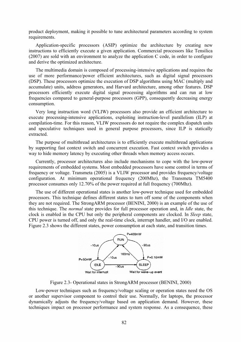
82

product deployment, making it possible to tune architectural parameters according to system requirements.

Application-specific processors (ASIP) optimize the architecture by creating new instructions to efficiently execute a given application. Commercial processors like Tensilica (2007) are sold with an environment to analyze the application C code, in order to configure and derive the optimized architecture.

The multimedia domain is composed of processing-intensive applications and requires the use of more performance/power efficient architectures, such as digital signal processors (DSP). These processors optimize the execution of DSP algorithms using MAC (multiply and accumulate) units, address generators, and Harvard architecture, among other features. DSP processors efficiently execute digital signal processing algorithms and can run at low frequencies compared to general-purpose processors (GPP), consequently decreasing energy consumption.

Very long instruction word (VLIW) processors also provide an efficient architecture to execute processing-intensive applications, exploiting instruction-level parallelism (ILP) at compilation-time. For this reason, VLIW processors do not require the complex dispatch units and speculative techniques used in general purpose processors, since ILP is statically extracted.

The purpose of multithread architectures is to efficiently execute multithread applications by supporting fast context switch and concurrent execution. Fast context switch provides a way to hide memory latency by executing other threads when memory access occurs.

Currently, processor architectures also include mechanisms to cope with the low-power requirements of embedded systems. Most embedded processors have some control in terms of frequency or voltage. Transmeta (2005) is a VLIW processor and provides frequency/voltage configuration. At minimum operational frequency (200Mhz), the Transmeta TM5400 processor consumes only 12.70% of the power required at full frequency (700Mhz).

The use of different operational states is another low-power technique used for embedded processors. This technique defines different states to turn off some of the components when they are not required. The StrongARM processor (BENINI, 2000) is an example of the use of this technique. The normal state provides for full processor operation and, in Idle state, the clock is enabled in the CPU but only the peripheral components are clocked. In Sleep state, CPU power is turned off, and only the real-time clock, interrupt handler, and I/O are enabled. Figure 2.3 shows the different states, power consumption at each state, and transition times.

Figure 2.3- Operational states in StrongARM processor (BENINI, 2000)

Low-power techniques such as frequency/voltage scaling or operation states need the OS or another supervisor component to control their use. Normally, for laptops, the processor dynamically adjusts the frequency/voltage based on application demand. However, these techniques impact on processor performance and system response. As a consequence, these

83

techniques require an integrated application and OS design in order to not disturb the real-time behavior that is commonly required for embedded applications.

2.2.2 Memory Memory design has an important impact on processor performance and power

consumption. For embedded processors, cache design is important because its influence on system power consumption represents about 50% of core power consumption (see Figure 2.4).

> 50%

Figure 2.4- Processor power-consumption (ZHANG; VAHID; LYSECKY, 2004)

Figure 2.5 presents work done by Zhang et al. (2004) showing the influence of cache size on global energy consumption. It can be seen that global energy is directly related to cache size. Initially, when cache size increases, global energy decreases because of fewer memory accesses. However, after a given point, the sheer influence of cache size dominates global energy consumption, despite a small number of memory accesses. The same scenario occurs for processor performance (HENNESSY, 2002). After a given point, an increase in cache size will not result in an increase in performance, because the application reaches a temporal and locality limit.

84

0

1

2

3

4

5

1KB

2KB

4KB

8KB

16K

B

32K

B

64K

B

128K

B

256K

B

512K

B

1MB

Cache Size

Ener

gy(J

)

Cache Memory Total

Figure 2.5- Cache size and its influence on system power consumption (ZHANG; VAHID;

LYSECKY, 2004)

Other techniques are available to decrease power consumption and execution time in memory hierarchies. Scratchpad or fast memories are small memories inside the processor core used to decrease access time and power consumption. The main difference with cache is that their contents are directly loaded by the application, making the programmer responsible for choosing which data and instructions are important in regards to fast memory. This technique makes execution time more predicable in comparison to caches, which can be polluted by other tasks. Jain et al. (2001) propose a technique to lock the cache lines, avoiding undesirable line substitution. In both techniques, knowledge of application behavior is necessary to optimize scratchpad and cache use.

2.2.3 Interconnection SoC interconnection design complexity is increasing due to the number of components

and sophisticated communication schemes. Ad-hoc solutions cannot deal with concerns regarding flexibility and design time, which can only be addressed by long-term solutions that can cope with future MPSoC requirements.

Point-to-point connections, shown in Figure 2.6(a), enable designs customized in terms of performance and predictability. However, design time and low reuse make point-to-point interconnections impracticable in future MPSoC designs.

Current MPSoC designs adopt bus-based (see Figure 2.6(b)) solutions (AMBA, 2007; CoreConnect, 2007). Due to scalability problems many variations, such as hierarchical buses and time-sliced arbitration, are proposed.

The network-on-chip (NoC) approach represents a long-term solution for MPSoC design. A NoC, as shown in Figure 2.6(c), provides the scalability and reuse necessary to future MPSoC designs. Predictability and real-time requirements call for NoC solutions with quality-of-service (QoS) capabilities. Currently, NoCs are a subject of intense research. However few real designs exist, due to high latency and area overhead when compared to other interconnection solutions.

85

uP M uPuP M

IP

E/S uP

uP

M

M(a) (b) (c)

uP M uPuP M

IP

E/S uP

uP

M

M(a) (b) (c)

Figure 2.6- Communication topologies (a) point-to-point, (b) bus-based connection, and (c) network-on-chip

To improve reusability, communication interconnection is provided in the form of IP components (AMBA, 2007; Sonics Backplane, 2007) that must be configured for a given application (for example, number of masters in a bus, switch buffer size in a NoC). This requires tools to explore the communication structure and to link application QoS requirements to the real implementation.

2.2.4 SoC Platforms The design of a new architecture involves non-recurring engineering (NRE) costs that are

not negligible in the overall cost of manufacturing and designing a SoC (MAGARSHACK, 2003). Due to these costs, developing a new architecture from scratch for each new product becomes unacceptable. Consequently, platforms are proposed to cover an application domain, and then tailored to a specific product.

Figure 2.7 shows the Nomadik (2007) platform targeted to mobile phones and multimedia PDAs. Nomadik is a multimedia platform composed of an ARM processor and audio and video accelerators (DSP processors). Many I/O interfaces, such as an LCD controller, USB, infrared, TV output, and flash card, are available. The memory organization is composed of embedded SRAM, secured RAM/ROM, and controllers for external Flash and DDR memories. The interconnection structure uses buses and bridges to decouple the main bus and to distribute communication. A DMA controller is available to manage the data transfers.

Figure 2.7- Nomadik architecture (NOMADIK, 2007)

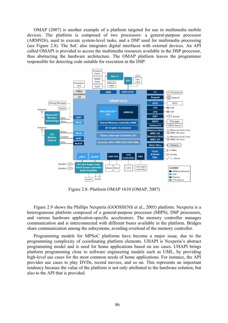
86

OMAP (2007) is another example of a platform targeted for use in multimedia mobile devices. The platform is composed of two processors: a general-purpose processor (ARM926), used to execute system-level tasks, and a DSP used for multimedia processing (see Figure 2.8). The SoC also integrates digital interfaces with external devices. An API called OMAPI is provided to access the multimedia resources available in the DSP processor, thus abstracting the hardware architecture. The OMAP platform leaves the programmer responsible for detecting code suitable for execution in the DSP.

Figure 2.8- Platform OMAP 1610 (OMAP, 2007)

Figure 2.9 shows the Phillips Nexperia (GOOSSENS et al., 2005) platform. Nexperia is a heterogeneous platform composed of a general-purpose processor (MIPS), DSP processors, and various hardware application-specific accelerators. The memory controller manages communication and is interconnected with different buses available in the platform. Bridges share communication among the subsystems, avoiding overload of the memory controller.

Programming models for MPSoC platforms have become a major issue, due to the programming complexity of coordinating platform elements. UHAPI is Nexperia’s abstract programming model and is used for home applications based on use cases. UHAPI brings platform programming close to software engineering models such as UML, by providing high-level use cases for the most common needs of home applications. For instance, the API provides use cases to play DVDs, record movies, and so on. This represents an important tendency because the value of the platform is not only attributed to the hardware solution, but also to the API that is provided.

87

Figure 2.9- Phillips Nexperia PNX8550 (GOOSSENS et al., 2005)

2.3 Software Design

Software development is becoming more and more time-consuming and will thus come to occupy most of the time spent to develop embedded systems. The heterogeneous nature of embedded systems makes traditional parallel approaches inadequate for the development of embedded software. Further, distributed programming models have the objective of providing portability and average performance, and do not fit well with embedded system requirements. The following sections describe parallel and distributed programming models used in embedded software development.

A programming model is a bridge between HW and SW. It abstracts the hardware for the software developer, using an API. An MPSoC requires programming models that provide the flexibility and heterogeneity of distributed systems, but also requires the intense processing of parallel applications and real-time constraints.

Some applications provide explicit parallelism and enable automatic parallelism extraction. Fine-grained parallelism can be explored by vector and VLIW architectures, where ILP is statically extracted without speculation of data or control. Tasks or threads employ coarse-grained parallelism. These loosely coupled threads require less synchronization and

88

communication. For example, encoders and decoders provide parallelism that can be extracted at fine and coarse grain.

The set of applications that can be automatically parallelized is limited. The research community claims that new programming paradigms are necessary to specify an application in a parallel manner. The heterogeneous nature of embedded systems, which entails a considerable amount of synchronization and communication, makes parallelization a difficult task.

Application software layers improve software development by spreading complexity over the different layers, as presented in Figure 2.10. In this layered approach, a middleware provides the services used by the application. This middleware is implemented on top of an operating system that provides basic services such as scheduling and synchronization. The hardware abstraction layer implements the low-level code to access the interconnect and other system components.

Applications Player, Game, Agenda

Middleware Corba, MPI, libraries

OS Scheduling, synchronization

HAL Drivers

Figure 2.10- Software application layers

Software development for MPSoCs imposes the same problems as those addressed in the domains of parallel and distributed systems. These include:

• Heterogeneity: different architectures have different ways of representing data (for instance, big and small endian architectures). The middleware and operating system need to deal with these low-level details.

• Scalability and flexibility: support for new functionalities; this avoids centralized solutions that can become the system bottleneck.

• Security: mobility and wireless communication capabilities are common in new products that require security features for data and communication.

• Fault tolerance: critical embedded applications must include fault tolerance techniques in their design.

• Concurrency: figuring out the details of data access and synchronization is a difficult and error-prone task that should not be left for the programmer. An adequate programming model addresses the problem of concurrency modeling.

• Transparency: transparency is desirable for system resource access, leaving component addressing for lower levels.

2.3.1 Programming Models Usually, the imperative programming model is extended to support parallelism and

concurrency. Threads divide the applications into concurrently computing entities. Shared

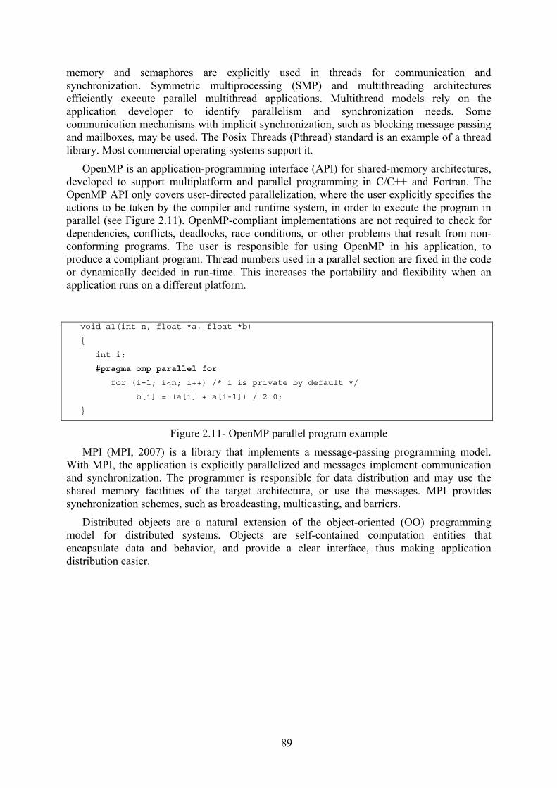
89

memory and semaphores are explicitly used in threads for communication and synchronization. Symmetric multiprocessing (SMP) and multithreading architectures efficiently execute parallel multithread applications. Multithread models rely on the application developer to identify parallelism and synchronization needs. Some communication mechanisms with implicit synchronization, such as blocking message passing and mailboxes, may be used. The Posix Threads (Pthread) standard is an example of a thread library. Most commercial operating systems support it.

OpenMP is an application-programming interface (API) for shared-memory architectures, developed to support multiplatform and parallel programming in C/C++ and Fortran. The OpenMP API only covers user-directed parallelization, where the user explicitly specifies the actions to be taken by the compiler and runtime system, in order to execute the program in parallel (see Figure 2.11). OpenMP-compliant implementations are not required to check for dependencies, conflicts, deadlocks, race conditions, or other problems that result from non-conforming programs. The user is responsible for using OpenMP in his application, to produce a compliant program. Thread numbers used in a parallel section are fixed in the code or dynamically decided in run-time. This increases the portability and flexibility when an application runs on a different platform.

void a1(int n, float *a, float *b)

{

int i;

#pragma omp parallel for

for (i=1; i<n; i++) /* i is private by default */

b[i] = (a[i] + a[i-1]) / 2.0;

}

Figure 2.11- OpenMP parallel program example MPI (MPI, 2007) is a library that implements a message-passing programming model.

With MPI, the application is explicitly parallelized and messages implement communication and synchronization. The programmer is responsible for data distribution and may use the shared memory facilities of the target architecture, or use the messages. MPI provides synchronization schemes, such as broadcasting, multicasting, and barriers.

Distributed objects are a natural extension of the object-oriented (OO) programming model for distributed systems. Objects are self-contained computation entities that encapsulate data and behavior, and provide a clear interface, thus making application distribution easier.

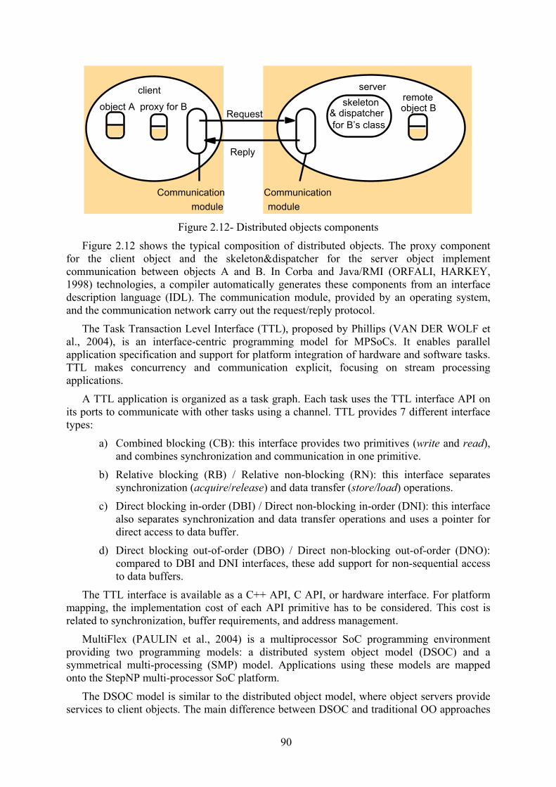
90

object A object BskeletonRequest

proxy for B

Reply

CommunicationCommunicationmodulemodule

for B’s class& dispatcher

remoteclient server

Figure 2.12- Distributed objects components

Figure 2.12 shows the typical composition of distributed objects. The proxy component for the client object and the skeleton&dispatcher for the server object implement communication between objects A and B. In Corba and Java/RMI (ORFALI, HARKEY, 1998) technologies, a compiler automatically generates these components from an interface description language (IDL). The communication module, provided by an operating system, and the communication network carry out the request/reply protocol.

The Task Transaction Level Interface (TTL), proposed by Phillips (VAN DER WOLF et al., 2004), is an interface-centric programming model for MPSoCs. It enables parallel application specification and support for platform integration of hardware and software tasks. TTL makes concurrency and communication explicit, focusing on stream processing applications.

A TTL application is organized as a task graph. Each task uses the TTL interface API on its ports to communicate with other tasks using a channel. TTL provides 7 different interface types:

a) Combined blocking (CB): this interface provides two primitives (write and read), and combines synchronization and communication in one primitive.

b) Relative blocking (RB) / Relative non-blocking (RN): this interface separates synchronization (acquire/release) and data transfer (store/load) operations.

c) Direct blocking in-order (DBI) / Direct non-blocking in-order (DNI): this interface also separates synchronization and data transfer operations and uses a pointer for direct access to data buffer.

d) Direct blocking out-of-order (DBO) / Direct non-blocking out-of-order (DNO): compared to DBI and DNI interfaces, these add support for non-sequential access to data buffers.

The TTL interface is available as a C++ API, C API, or hardware interface. For platform mapping, the implementation cost of each API primitive has to be considered. This cost is related to synchronization, buffer requirements, and address management.

MultiFlex (PAULIN et al., 2004) is a multiprocessor SoC programming environment providing two programming models: a distributed system object model (DSOC) and a symmetrical multi-processing (SMP) model. Applications using these models are mapped onto the StepNP multi-processor SoC platform.

The DSOC model is similar to the distributed object model, where object servers provide services to client objects. The main difference between DSOC and traditional OO approaches

91

such as Java/RMI and Corba is that hardware accelerators provide the support for message passing, resulting in low overhead. There are two hardware accelerators: a message passing engine (MPE) and an object request broker (ORB). The MPE is used to translate messages into a portable representation and to transmit the request through the NoC, as shown in Figure 2.13. Scheduling requests to servers, the ORB component coordinates object communication. ORB supplies the load balancing over system resources, thus providing parallel execution and scalability. An interface description language called SIDL (SystemC interface description language) is used to generate software drivers to access the MPE for software components. For the HW components, a tool generates the data conversion hardware and links it to the NoC interface.

Figure 2.13- DSOC model for platform mapping (PAULIN et al., 2004)

The SMP model is based on the POSIX Threads model. It supports concurrent execution using shared memory. Monitors and signals are provided for communication and synchronization. The SMP model combines a lightweight software layer and a hardware concurrency engine (CE). The CE controls the monitors and signal implementation as well as the hardware context switch, thus yielding low cost implementation.

The DSOC/SMP model proposes the hardware implementation of key components of a distributed and parallel programming model, resulting in low overhead. This enables the systematic mapping of the DSOC/SMP application to the StepNP platform. On the other hand, this hardware support decreases software portability, and mapping to another platform will necessitate a new hardware and software interface design.

2.4 ROSES MPSoC Design Environment

ROSES is a component-based environment for system-level design. It provides HW/SW interface abstraction, thus decreasing the complexity of MPSoC design.

92

The ROSES design flow starts with a virtual architecture model that corresponds to the “golden” architecture obtained from the architecture exploration step. This virtual architecture model allows automatic generation of communication coprocessors/controllers (wrappers), device drivers, operating systems, and application programming interfaces.

The virtual architecture model is a set of virtual modules interconnected using point-to-point virtual channels and/or a communication interconnect IP. The goal is to produce a synthesizable RTL model of the MPSoC platform that is composed of processor cores, IP cores, the communication interconnect, and HW/SW wrappers. Virtual component interfaces are used to automatically generate application-specific hardware and software wrappers (see Figure 2.14). Software written for the virtual architecture specification can run without modification on the implemented platform because the generated custom operating system provides the same APIs.

Figure 2.14- ROSES design flow (CESARIO et al., 2002)

The ROSES environment uses an extensible and multi-level design representation called COLIF. This design meta-model based on XML allows description of hierarchical components and abstract HW/SW interfaces at different design levels. All of the tools in the ROSES design flow use the COLIF meta-model.

2.4.1 HW/SW Interface Abstraction The virtual architecture represents a system as an abstract netlist of virtual components

(see Figure 2.15). A virtual component consists of an internal component (or module) and its wrapper. The internal component contains a set of software tasks or represents a hardware function. The wrapper adapts accesses from the internal component to the external channels connected to the virtual component. The internal component and external channel(s) can be different in terms of communication protocol, abstraction level, and specification language. The wrapper is a set of virtual ports that contain internal and external ports. The internal and external wrappers’ ports abstract the HW/SW interfaces that will be refined to generate the final implementation system.

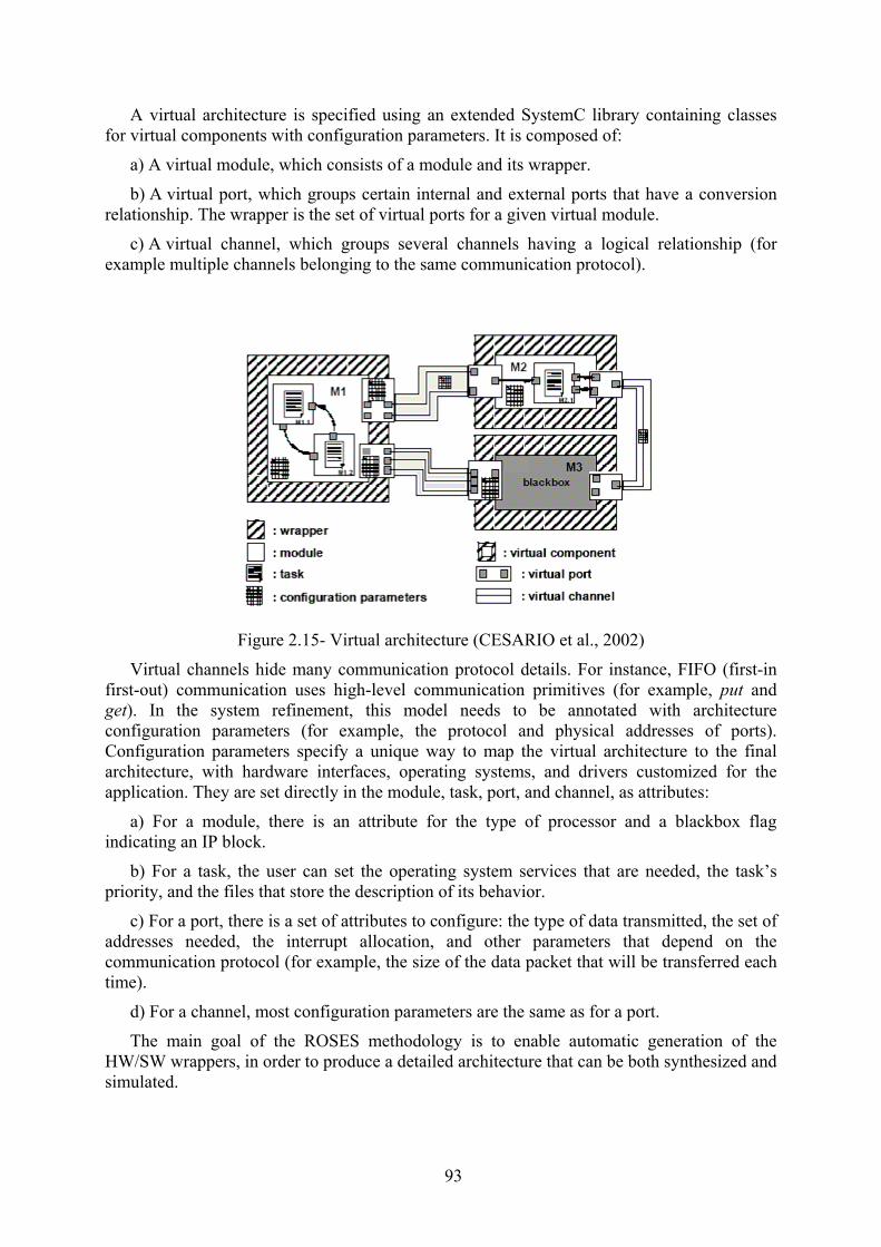
93

A virtual architecture is specified using an extended SystemC library containing classes for virtual components with configuration parameters. It is composed of:

a) A virtual module, which consists of a module and its wrapper.

b) A virtual port, which groups certain internal and external ports that have a conversion relationship. The wrapper is the set of virtual ports for a given virtual module.

c) A virtual channel, which groups several channels having a logical relationship (for example multiple channels belonging to the same communication protocol).

Figure 2.15- Virtual architecture (CESARIO et al., 2002)

Virtual channels hide many communication protocol details. For instance, FIFO (first-in first-out) communication uses high-level communication primitives (for example, put and get). In the system refinement, this model needs to be annotated with architecture configuration parameters (for example, the protocol and physical addresses of ports). Configuration parameters specify a unique way to map the virtual architecture to the final architecture, with hardware interfaces, operating systems, and drivers customized for the application. They are set directly in the module, task, port, and channel, as attributes:

a) For a module, there is an attribute for the type of processor and a blackbox flag indicating an IP block.

b) For a task, the user can set the operating system services that are needed, the task’s priority, and the files that store the description of its behavior.

c) For a port, there is a set of attributes to configure: the type of data transmitted, the set of addresses needed, the interrupt allocation, and other parameters that depend on the communication protocol (for example, the size of the data packet that will be transferred each time).

d) For a channel, most configuration parameters are the same as for a port.

The main goal of the ROSES methodology is to enable automatic generation of the HW/SW wrappers, in order to produce a detailed architecture that can be both synthesized and simulated.

94

2.4.2 HW Wrapper Generation - ASAG Hardware wrapper generation assembles the hardware interface from a library of

components, using the virtual architecture specification. Architecture configuration parameters are used to instantiate library components; they are the result of decisions made during system architecture exploration. The library contains generalized descriptions of hardware components in a macro language and is composed of two parts: the processor library and the protocol library. The former contains local template architectures for processors with four types of elements: processor cores, local buses, local IP components (for example local memory, address decoder, and coprocessors), and processor adapters. The latter consists of a list of channel adapters. Each channel adapter has simulation and synthesis models that are parameterized (by channel parameters such as direction, storage size, and data type), much like the elements in the processor library.

Figure 2.16- Hardware wrapper architecture (CESARIO et al., 2002)

Hardware wrappers are implemented as communication co-processors, as shown in Figure 2.16. The processor adapter interconnects the processor bus with the channel adapters. This solution enables the separation between communication and computation, releasing the processor to execute in parallel with the communication.

2.4.3 SW Wrapper Generation – ASOG

The software wrapper generator produces an application-specific operating system tailored to the software module(s) that run(s) on each target processor (GAUTHIER et al., 2001). It uses an operating system library organized in three parts: APIs, communication/system services, and device drivers. Each part contains elements that will be used in a given software layer of the generated OS.

The API implements the interface between the application and the OS services. The system services implement basic services such as scheduling, synchronization, and memory management. Device drivers contain the low level code used to access the system components (for example, memories and hardware IP components).

The library is organized as services that have dependencies between them. For instance, communication services are dependent on the I/O services. The virtual architecture describes the services required by the application, and these dependencies are used to keep the size of the generated OS at a minimum. The generation flow is shown in Figure 2.17.

95

Figure 2.17- Application-specific OS generation flow (GAUTHIER et al., 2001)

Most of the library components are written in C language, which makes porting to different architectures easier. Assembler code is used only in very specific codes, such as the boot code, context switch, and device drivers, which represent a small part of the whole library.

2.4.4 Simulation Model Generation – CosimX The CosimX tool provides heterogeneous multi-level simulation generation

(NICOLESCU et al., 2002; SARMENTO et al., 2004). For the interfaces, at different levels, it generates a simulation with wrappers (from a library) to adapt the protocol, as presented in Figure 2.18.

CosimX produces an executable model that is used to validate the internal model. This executable model is composed of a SystemC simulator that acts as a master for other simulators. A variety of simulators can participate in this co-simulation: SystemC, VHDL, Verilog, and instruction-set simulators. Co-simulation wrappers have the same structure as hardware wrappers, with simulation adapters instead of processor adapters, and simulation models of channel adapters. In the co-simulation wrapper library, there are simulation adapters for the different simulators supported. There are also channel adapters that implement all supported communication protocols in different languages.

96

In terms of functionality, the co-simulation wrapper transforms channel access(es) via internal port(s) into channel access(es) via external port(s) using the following functional chain: channel interface, channel resolution, data conversion, and module communication behavior.

Figure 2.18- Executable model generation in CosimX (SARMENTO et al., 2004)

Internal ports use the communication API (for example, put and get in FIFO channels) to exchange the data. At virtual architecture level, the channel interface provides the implementation of these channel functions. Data conversion is required, since different abstraction levels can use different data types to represent the same data.

At BFM-level, an operating system and hardware wrappers implement the communication API. In this case, the co-simulation wrappers implement the ISS integration in the co-simulation environment. The co-simulation bus used for synchronization and data exchanges is implemented using inter-process communication (IPC).

2.5 Performance Estimation

The development of performance estimation and analysis tools is an active research area. Software performance estimation methods are used mainly for worst-case execution analysis (WCET), architecture exploration, and micro-architecture tuning. In MPSoC design, performance estimation becomes complex and requires system-level methods allowing an integrated analysis of different processors, hardware components, and interconnection.

In Section 2.5.1, we will present methods for estimation of software performance in a given architecture. These tools are proposed to provide fast estimation in the context of design space exploration. Section 2.5.2 discusses related work in the area of integrated hardware and software performance estimation. These works aim to provide global estimation that considers multiprocessor and communication issues.

97

2.5.1 Software Performance Estimation This section presents estimation techniques for software running in a given processor.

Simulation techniques offer accurate software performance estimation with high costs and considerable modeling efforts. Analytic models estimate software performance using abstract models. Although they are fast, the main challenge with analytic models is to derive an accurate model for advanced processor architectures. Complementary to simulation and analytic-based methods, worst-case execution analysis (WCET) techniques aim to automatically discover the worst execution path, which is important for real-time analysis.

2.5.1.1 WCET Estimation

Real-time system and scheduling analysis (PUSCHNER; BURNS, 2000) stimulates the development of worst-case execution time (WCET) solutions. Given a set of tasks T, described as a tuple {D, P, E} that represents the deadline, period, and execution time, respectively, the schedulability test determines if a schedule policy satisfies the temporal requirements. In this case, WCET tools give the task execution time (E).

The application real-time analysis is validated in two phases. Initially, the WCET of each task is calculated, and, subsequently, the schedulability test determines the real-time properties. WCET may be obtained using cycle-accurate simulators of the target processor. For simple tasks, this technique is straightforward, but in complex applications, finding the inputs that will result in the worst-case execution time is difficult and error-prone.

In worst-case execution time (WCET) calculation, it is necessary to find out the sequence of basic blocks that is responsible for the worst case. The static extraction of the execution flow allows the WCET calculation, even for applications where the execution behavior is dependent on the input data.

Li and Malik (LI; MALIK, 1995) propose a static analysis method using a technique called implicit path enumeration, which determines the execution number of each basic block in the worst-case. These limits are calculated by linear equations obtained from structural and functional analysis. Structural restrictions are generated from a control flow graph (CFG) analysis. Functional restrictions are given by the user and describe the information that cannot be obtained from the CFG, such as loop limits and false paths. A linear programming method maximizes these equations and calculates the WCET.

Figure 2.19 describes a C code example and shows its control flow graph. Equations 2.2 to 2.5 represent structural and functional restrictions. Equation 2.2 represents a functional restriction that describes the maximum value of the while loop (in the example, the loop limit is 100). Using the associated cost of each basic block equation (ci), a linear programming technique is employed to maximize equation 2.1, using the functional and structural restrictions described by linear equations.

Cycles= ∑=

n

iii dc

0* (2.1)

d2 <= 100 (2.2)

x2= d1+ d7 (2.3)

x3= d2= d3+ d4 (2.4)

x6=d5+d6= d7+d9 (2.5)

98

The WCET calculation may be extremely pessimistic in cases where the functional restrictions were imprecisely defined. The programmer must know the application and provide precise functional restrictions. Moreover, the method can be pessimistic in an additional way, since it considers that the execution cost of a basic block (ci) is fixed.

S int counting(vector v, int n, int value) {

int i, j; i=0; j= 0; while (i < n) {

if ( v[i ] == value) {

j++; } else {

j -- ; }

i++; } return j;

}

i=0; j= 0;

while (i < n)

if ( v[j]==value)

j++ j --

i++

return j

E

d1

d2

d3 d4

d5 d6

d7

d9

d8

X1

X2

X3

X4 X5

X6

X7

Figure 2.19- Static WCET analysis

Wolf and Ernst (WOLF; ERNST, 2000) present a method to reduce the linear (in) equations – thus reducing complexity – by trying to extract a single feasible path. A single feasible path can be extracted when the program execution is input-independent. Even though this is not the case for all programs, some subparts (such as kernels in digital signal processing algorithms) can be classified as a single path. Moreover, Wolf and Ernst’s work does not use the worst-case, but instead uses intervals that are calculated considering that a basic block execution cost varies. Intervals give more accurate results because they use an accurate basic block execution cost.

Static analysis can supply other information that is also relevant for performance estimation in the presence of complex architectural features. In (LI; MALIK; WOLFE, 1995) and (HERGENHAN; ROSENSTIEL, 2000), the number of misses in the instruction cache is obtained by applying linear equations. Li et al. (2003) describe a method that models the impact of speculative execution based on the number of misses in the instruction cache. The number of misses of the branch predictor may also be statically obtained, as presented in (COLIN; PUAT, 2000). These predictions increase the precision of the execution time calculation of each basic block, since this calculation only uses local information. In this phase, cycle-accurate simulators may be used (LI; MALIK, 1995; WOLF, 2000), alternatively, but at a higher cost. Employing more abstract processor models reduces complexity and facilitates retargeting of the estimation method for different processors (ENGBLOM et al., 2001; SCHNEIDER; FERDINAND, 1999; LIM et al, 1998).

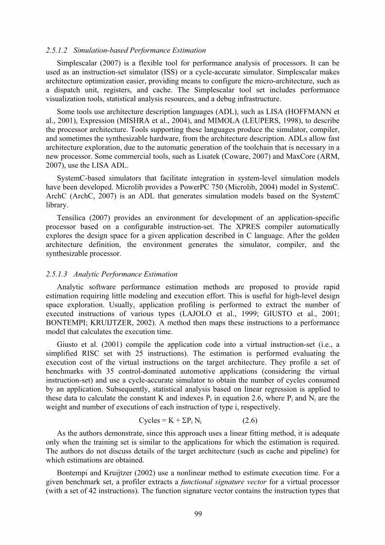
99

2.5.1.2 Simulation-based Performance Estimation

Simplescalar (2007) is a flexible tool for performance analysis of processors. It can be used as an instruction-set simulator (ISS) or a cycle-accurate simulator. Simplescalar makes architecture optimization easier, providing means to configure the micro-architecture, such as a dispatch unit, registers, and cache. The Simplescalar tool set includes performance visualization tools, statistical analysis resources, and a debug infrastructure.

Some tools use architecture description languages (ADL), such as LISA (HOFFMANN et al., 2001), Expression (MISHRA et al., 2004), and MIMOLA (LEUPERS, 1998), to describe the processor architecture. Tools supporting these languages produce the simulator, compiler, and sometimes the synthesizable hardware, from the architecture description. ADLs allow fast architecture exploration, due to the automatic generation of the toolchain that is necessary in a new processor. Some commercial tools, such as Lisatek (Coware, 2007) and MaxCore (ARM, 2007), use the LISA ADL.

SystemC-based simulators that facilitate integration in system-level simulation models have been developed. Microlib provides a PowerPC 750 (Microlib, 2004) model in SystemC. ArchC (ArchC, 2007) is an ADL that generates simulation models based on the SystemC library.

Tensilica (2007) provides an environment for development of an application-specific processor based on a configurable instruction-set. The XPRES compiler automatically explores the design space for a given application described in C language. After the golden architecture definition, the environment generates the simulator, compiler, and the synthesizable processor.

2.5.1.3 Analytic Performance Estimation

Analytic software performance estimation methods are proposed to provide rapid estimation requiring little modeling and execution effort. This is useful for high-level design space exploration. Usually, application profiling is performed to extract the number of executed instructions of various types (LAJOLO et al., 1999; GIUSTO et al., 2001; BONTEMPI; KRUIJTZER, 2002). A method then maps these instructions to a performance model that calculates the execution time.

Giusto et al. (2001) compile the application code into a virtual instruction-set (i.e., a simplified RISC set with 25 instructions). The estimation is performed evaluating the execution cost of the virtual instructions on the target architecture. They profile a set of benchmarks with 35 control-dominated automotive applications (considering the virtual instruction-set) and use a cycle-accurate simulator to obtain the number of cycles consumed by an application. Subsequently, statistical analysis based on linear regression is applied to these data to calculate the constant K and indexes Pi in equation 2.6, where Pi and Ni are the weight and number of executions of each instruction of type i, respectively.

Cycles = K + ΣPi Ni (2.6)

As the authors demonstrate, since this approach uses a linear fitting method, it is adequate only when the training set is similar to the applications for which the estimation is required. The authors do not discuss details of the target architecture (such as cache and pipeline) for which estimations are obtained.

Bontempi and Kruijtzer (2002) use a nonlinear method to estimate execution time. For a given benchmark set, a profiler extracts a functional signature vector for a virtual processor (with a set of 42 instructions). The function signature vector contains the instruction types that

100

appear in the code and the number of times each instruction type is executed. This functional signature is theoretically independent of the target architecture, so it can be reused for estimation with different processors. The authors, however, do not discuss the impact of using this functional signature to estimate performance for a processor of an architectural type that is different from the virtual processor upon which the profiler is based. Their estimation method is also based on the architectural signature of the target processor. They propose two parameters that define this signature: the number of memory wait cycles and the ratio between the CPU clock and bus clock. They present estimation results for a MIPS R3000.

Bontempi and Kruijtzer use a training-and-test approach. In the test phase, they apply a modeling technique called lazy learning to choose an estimation function that is based on a criterion of neighborhood between the application and the training set. This function, which may be locally linear, only uses points of the training set that are near of the application estimation function. The inputs for this phase are the functional and architectural signatures, and the number of clock cycles needed to execute each application in the benchmark set. The number of clock cycles is obtained from a cycle-accurate simulation in the target processor. The authors propose a training method based on splitting the benchmarks into two disjoint sets for training and testing. They report a mean error of 8.8% in the estimations, for a set of 6 benchmarks, each one executed with 15 different input data sets. However, they do not mention the size of the training and test sets.

Bammi et al. (2000) compare an annotation technique that uses a virtual instruction-set with another annotation technique applied at object-code level. The former translates the C code to a virtual instruction (VI) set. Each instruction in VI has a cost associated to the target architecture that is obtained either by simulation or by a statistical method, as presented in Giusto’s work. The second method (that is, the one at object-code level) uses compiled simulation, where the assembler code is translated to a simulation code using delay annotation that will be executed in the host machine. The authors report that the object-based approach provides more accurate results because it can capture compiler optimizations. They report results using a MIPS R3000 processor for a producer/consumer application. The virtual instruction method results in errors between -0.29% to -80% compared to cycle-accurate simulation. The object-code method gives errors between -0.29% and -10.5%.

Ipek et al. (2006) propose a neural network estimator used to explore application performance, when executing under different architecture configurations. The neural network inputs are the architectural parameters and the output is the cycles per instruction (CPI). The authors evaluate different memory hierarchy and processor.

For memory hierarchy, the following parameters were evaluated: L1 DCache Size, L1 DCache Block Size, L1 DCache Associativity, L1 Write Policy, L2 Cache Size, L2 Cache Block Size, L2 Cache Associativity, L2 Bus Width, and Front Side Bus Frequency. These different parameters require 20736 simulations per benchmark. The processor architecture was evaluated with respect to the following parameters: Fetch/Issue/Commit Width, Frequency, Branch Predictor, Branch Target Buffer, ALU/FPU unit number, Reorder Buffer Size, Register File, and LD/ST Queue. The combination of these parameters yields 20736 different configurations; and consequently, that many cycle-accurate simulations are needed to explore the design space.

In a case study with SPEC 2000 benchmarks, the authors obtained a mean error ranging from 2% to 4%, using just 4% of the total design space for the training set. Also, the training time was around 2 minutes, using a cluster with 10 nodes. In addition, the authors evaluated the technique in a multiprocessor architecture (CMP, in this case). The parameters evaluated were Core configuration (In-order, out-of-order), Issue width, Number of cores,

101

SMT contexts per core, Off-chip bandwidth, Frequency, L2 Cache Size, L2 Cache Block Size, and L2 Cache Associativity. For the case study, applications from the SPEC OMP and parallel NAS benchmarks were employed. With 1% of the total design space used for the training set, estimation errors of up to 6.4% were obtained.

2.5.2 Integrated Hardware and Software Performance Estimation Aside from processor-level tools, new integrated hardware and software tools and methods

are necessary to estimate performance of whole systems, including hardware components, software components, and their interfaces.

2.5.2.1 Simulation-based Performance Estimation

Virtual prototypes are simulation models that enable the integrated validation of hardware and software components. They integrate an instruction-set simulator with hardware simulation models such as memory, bus, peripheral, and IP components. Environments for modeling and simulation of virtual prototypes based on SystemC, such as MaxSim (ARM, 2007), Coware ConvergenSC (Coware, 2007), and Synopsys System Studio (Synopsys, 2007), provide a rich set of components that can be extended by user-defined SystemC modules. Some tools support the RTL synthesis for these library components, providing an automatic path to the silicon. For instance, Synopsys CoreAssembler generates the RTL interconnection structure from virtual prototypes described in MaxSim (GRUN et al., 2005).

Other virtual prototype simulators, such as SIMICS (2007), use functional models for the processor, buses, and hardware components. Functional models provide reasonable speed to execute real workloads. Some works have proposed the integration of functional system simulators and cycle-accurate processor simulators such as Simplescalar (MAUER; HILL; WOOD, 2002). Chen et al. (2003) also integrated power estimators, providing integrated performance/power estimation.

Fummi et al. (2004) present two methods for the integration of instruction-set simulators (ISS) in SystemC models. The authors use the GNU debbuger (gdb) as instruction set simulator together with SystemC simulation. The first method uses a breakpoint in SW to stop the execution and to synchronize with the SystemC kernel. The second uses the adapted OS drivers that stop software execution and communicate with SystemC when an I/O operation is made. In both cases, changes are necessary in the SystemC simulation kernel to support synchronization and data transfer.

MPARM (BENINI et al., 2005) is an environment for MPSoC design exploration using SystemC. It is a complete platform solution for MPSoC simulation composed of processor models (ARM), bus models (AMBA), memory models, hardware support for SMP (hardware semaphores), and a software development toolset including a C compiler and an operating system (UCLinux). Hardware components, such as memories and the AMBA bus model, are all written in SystemC. The AMBA bus model allows multiple masters and slaves and can be configured in terms of arbitration policy. A cycle-accurate instruction-set ARM simulator developed in C++ is encapsulated in a SystemC wrapper and integrated into the platform. The wrapper realizes the interface and synchronization between the instruction-set simulator and SystemC simulation framework. This integration allows plugging the ISS into a system simulation activated by a common system clock, thus providing a consistent and synchronized hardware and software multiprocessor simulation. Figure 2.20 shows an architecture example

102

composed of two ARM processors, the AMBA bus, two memory modules, and hardware semaphores.

Figure 2.20- MPARM system architecture example (BENINI et al., 2005)

In MPARM, the software tool chain was extended to support multiprocessor execution. This includes special memory mapping for processor initialization, given that following initialization, each processor has to branch to its own initialization routine. The multiprocessor shared-memory architecture supports atomic memory operations (test&set instructions) implemented by hardware semaphores. These hardware semaphores affect operating system implementation; in the MPARM environment, a Linux-based OS (UCLinux) was adapted to support the multiprocessing architecture.

MPARM provides support for performance analysis. The performance statistics include cache miss/hit rate, as well as bus contention and average transfer waiting time. These statistics are used to explore the bus arbitration policy in the AMBA bus.

Meyr et al. (WIEFERINK et al., 2004) propose a link between simulation models generated with LISA and SystemC system-level simulation. The goal is to explore the processor and communication jointly, using a system-level approach. The integrated co-verification environment provides a way to analyze software performance, for example CPU load and RTOS overhead. Furthermore, shared resources (e.g., memory and buses) directly affect SW performance, and isolated analysis of a single processor hides potential problems and bottlenecks.

The processor simulator is modeled at instruction-accurate or cycle-accurate level. Instruction-accurate models execute the full instruction-set but ignore pipeline effects. In contrast, a cycle-accurate model fully simulates the pipeline stages and the stalls due to memory accesses. The processor generated from LISA is encapsulated in a SystemC wrapper and connected with the rest of the system using TLM or RTL interfaces.

TLM channels provide high-speed simulation. Such channels may be modeled as functional or bus cycle-accurate (BCA). Functional TLM interfaces use read and write operations to access the SoC bus. Blocking interfaces can be used to simulate access latency.

103

Bus cycle-accurate (BCA) interfaces provide cycle level detail including bus requests, data transfer, and device latencies.

The authors propose different combinations of processors and bus model abstraction levels (see Figure 2.21):

a) Processor stand-alone simulator;

b) Instruction-accurate processor and functional communication;

c) Cycle-accurate processor model and functional communication;

d) Cycle-accurate processor model and BCA communication;

e) Cycle-accurate processor model and RTL pin-level communication;

f) RTL processor and RTL pin-level communication.

Figure 2.21- LISA simulation and SystemC integration levels (WIEFERINK et al., 2004)

The stand-alone simulator (level 1) disregards communication and conflicts in shared resources, considering only the isolated software execution. Clearly this method is inaccurate for MPSoC designs. Level 2 already considers the system-level simulation, and the software uses the instruction-accurate simulators with functional interfaces with the rest of the system. These interfaces model the operations without considering timing concerns. In the next level, the instruction-accurate simulator is replaced by a cycle-accurate one (level 3), which precisely models the pipeline, branch predictors, and other effects. In level 4, communication is modeled as cycle-accurate using transaction channels called BCA (bus cycle-accurate). In the next level, the interfaces are refined using a full pin interface (level 5). The last step uses synthesizable component models using hardware description language simulators.

Posadas et al. (2004) propose a performance estimation method (using SystemC) that is based on a performance-annotated library. The authors use code segments instead of basic blocks. A code segment is a set of basic blocks without wait statements or channel accesses. As such, the SystemC process does not interact with the simulation kernel.

To consider the execution delay, the authors propose a method based on redefinition of C++ classes that contribute to the execution time with the performance annotation. The

104

redefined class executes the behavior normally and additionally calculates the execution delay (for instance, in the Integer class, the operator + realizes the sum and computes the delay of this operation). At the end of the segment, when the execution reaches a wait statement or a channel access, the accumulated delay is used as the execution time. For the hardware, the same method is used, but it can consider the concurrent segment execution. Channels also use annotation to compute operating system overhead.

The authors consider that the platform vendor should provide performance values annotated in each object. Errors below 4.5% in the SW and 8.2% in the HW were obtained, experimentally, using a voice decoder for GSM applications composed of 4 processes mapped into a RISC processor and a hardware accelerator. The authors report a simulation speed gain of 142 times compared to ISS simulation.

2.5.2.2 Analytical-based Performance Estimation

Analytical and formal methods are proposed to find a way around long simulation time and to avoid building an executable model. Such tools are proposed to verify system performance and certain properties, such as the maximum throughput, maximum delays, and buffer utilization, among others. Usually, analytical methods are used in design space exploration where absolute precision is not required, and where one only seeks to obtain a good idea of the performance (in relative terms) of alternative architectures.

Chakraborty et al. (2003) present a framework to analyze system properties modeled as event streams, based on real-time calculus. This framework has been applied to the design exploration of network processor architectures (THIELE et al., 2002), determining the cost/performance trade-off of different configurations of HW and SW components.

Ritcher et al. (2003) propose a formal approach used to verify the schedulability properties of heterogeneous multiprocessors systems. The key idea is to use the current formalisms for individual components and extend them in a compositional model for global MPSoC analysis. The individual analysis methods include well-known scheduling analysis techniques such as RMS (rate monotonic scheduling), EDF (earliest deadline first), and TDMA (time-division multiple accesses). These analysis techniques model the task or communication activation as event streams. The authors describe that the main problem in the compositional model is that the output event models are usually not supported as input models. To solve this problem, a set of event model interfaces (EMIF) and event adaptation functions (EAF) is used to automatically adapt the output event stream to match up with an established input event model.

Figure 2.22 presents two adaptations of an output event model to an input event model. In the example, C2 and C3 are accesses, through the interconnection, to an HW IP component and a DSP processor. In the DSP component, the well-established formalism uses the simple periodic model as input, which represents the processing execution when a given data quantity is available. Therefore, the output model from the interconnection is represented as a periodic event stream with jitter. To match both models, the interface (EMIF and EAF) adapts the periodic bursts using buffers and activates the DSP processor when the data quantity is sufficient. In this case, the formal model provides the execution bounds and helps optimize the buffer requirements.

105

Figure 2.22- Adaptation between event models in SymTA/S (RITCHER et al., 2003)

Russell and Jacome (2003) present a method based on abstract performance models and application scenarios. An application scenario is a defined path in the control flow graph that expresses the most important application characteristics. The scenario is statically extracted from user input constraints. The input constraints are propagated to prune the nodes in the infeasible paths. From initial constraints, other constraints are derived and propagated in an iterative process. The iterative process may require user interaction to define manual constraints resulting in a unique CFG (control flow graph) path called ‘scenario’. A trace is generated using this scenario and the performance is evaluated using an abstract cost function for each component. Cost functions are determined from component properties, architecture features, and values supplied by the designer. For instance, the processor cost function calculates the cycles needed to execute a given instruction. To calculate memory access costs, the values are derived from the interconnection topology in combination with databook values (for example, access time). The structural architecture adds the influence of components that are traversed during an operation. For example, in a memory access, buses and memory controllers are used, and their influence is accounted for in the performance estimation. The authors present a case study of a network interface. The work analyzes two different memory organizations using the Intel i960 as target architecture. An estimation error of up to 20% is reported.

2.5.2.3 Hybrid and Trace-based Performance Estimation

In order to find a way around long simulation time, hybrid trace-based methods combining simulation and profiling are proposed. The profiling information obtained from a generic architecture is used to estimate the application performance without necessity of rerunning the simulation for each different configuration.

The SPADE environment (LIEVERSE et al., 2001) proposes a trace-based performance estimation method with a clear separation between functionality and architecture. The application is modeled as Kahn networks. A Kahn model is composed of parallel processes that communicate via unbounded FIFO channels. The application-programming interface (API) is composed of three functions: read, write, and execute. During the Kahn model execution a trace is generated, taking into account communication workload (read and write operations) and computation workload (execute operations). The architecture is assembled

106

using blocks that model different resources such as processing, communication, and memory resources. A processing resource is composed of a trace-driven execution unit, which interprets trace entries and I/O interfaces that are connected to a specific communication resource.

In the SPADE environment, following application and architecture definition, the mapping is realized. Each process is mapped onto a processing resource. The Kahn channels are mapped to a combination of communication and memory resources. The simulation is then performed and the application trace is applied to the architecture model. The performance data collected during simulation include the utilization and stall cycles that are due to I/O operations. For communication resources, the performance data include the amount of data sent over the bus, the utilization, and the wait cycles. The application trace may be reused for different architectures, enabling fast design exploration of different design points.

Mohanty and Prasanna (2002) propose a high-level performance estimator called HiPerE to guide performance evaluation and mapping in SoC architectures. The input for the HiPerE simulator is an architecture and application described in GenM (Generic model). A GenM models the SoC architecture capabilities that will be used to optimize the application mapping. The SoC architecture consists of three components: a processor, reconfigurable logic, and memory. The GenM describes the different architecture configurations, such as voltage operations of the processor, power states for the memory, and reconfiguration cost for the reconfigurable logic. In GenM, an application is described as a task graph. For each task, a set of performance parameters is given by the designer, for instance, the amount of input and output data to/from memory, and the time and energy for executing the task at a given voltage. The initial estimations can be obtained by analytic methods. The authors show an example describing performance and energy as a function of operational frequency. This general function is derived just by using fewer benchmark runs, as proposed in (GIVARGIS; VAHID, 2002).

To improve the accuracy of these initial estimations, the authors propose linking GenM with a simulation-based framework in order to estimate the performance of an individual task with more accuracy. This framework, called MILAN, takes the task description (in C) and generates the scripts as well as the configuration files necessary to launch the simulator and to obtain the performance and power estimation. The simulators used to obtain these data were SimpleScalar and Wattch (in this case, for the MIPS 3000 architecture).

Using a symbolic simulator, HiPerE can verify the performance (latency in completing the task graph execution) and the energy for a given mapping. This fast symbolic simulation enables system optimization in terms of power consumption or performance.

Lahiri et al. (2001) present a trace-based method to explore a communication architecture consisting of a network of shared and/or dedicated communication channels and hierarchical channels connected by bridges.

The method comprises two steps, as shown in Figure 2.23. In the first step, HW/SW partitioning and processor selection is performed. Communication is modeled at an abstract level by the exchange of events or tokens. The HW/SW co-simulation generates timing inaccurate system execution traces that take into account the communication architecture. The execution trace is represented by a CAG (communication analysis graph) that captures computations, communications, and synchronization.

In the second phase, the designer specifies the communication architecture and the proposed tool carries out the system performance analysis. The communication architecture is modeled as a set of parameterized shared buses (with parameters such as width, speed, and

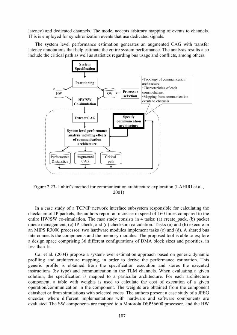
107

latency) and dedicated channels. The model accepts arbitrary mapping of events to channels. This is employed for synchronization events that use dedicated signals.

The system level performance estimation generates an augmented CAG with transfer latency annotations that help estimate the entire system performance. The analysis results also include the critical path as well as statistics regarding bus usage and conflicts, among others.

SystemSpecification

Partitioning

HW SWHW/SW

Co-simulation

Extract CAG

Processorselection

System level performance analysis inclufing effects

of communication architecture

Performance& statistics

AugmentedCAG

Critical path

Specify communication

architecture

•Topology of communication architecture•Characteristics of each comm.channel•Mapping from communication events to channels

Figure 2.23- Lahiri’s method for communication architecture exploration (LAHIRI et al., 2001)

In a case study of a TCP/IP network interface subsystem responsible for calculating the checksum of IP packets, the authors report an increase in speed of 160 times compared to the entire HW/SW co-simulation. The case study consists in 4 tasks: (a) create_pack, (b) packet queue management, (c) IP_check, and (d) checksum calculation. Tasks (a) and (b) execute in an MIPS R3000 processor; two hardware modules implement tasks (c) and (d). A shared bus interconnects the components and the memory modules. The proposed tool is able to explore a design space comprising 36 different configurations of DMA block sizes and priorities, in less than 1s.

Cai et al. (2004) propose a system-level estimation approach based on generic dynamic profiling and architecture mapping, in order to derive the performance estimation. This generic profile is obtained from the specification execution and stores the executed instructions (by type) and communication in the TLM channels. When evaluating a given solution, the specification is mapped to a particular architecture. For each architecture component, a table with weights is used to calculate the cost of execution of a given operation/communication in the component. The weights are obtained from the component datasheet or from simulations with selected codes. The authors present a case study of a JPEG encoder, where different implementations with hardware and software components are evaluated. The SW components are mapped to a Motorola DSP56600 processor, and the HW

108

component cost is obtained from the manually implemented RTL models. The estimation from the dynamic profiling gives a maximum error of 12.5% compared to the cycle-accurate simulation.

The Platune environment (GIVARGIS; VAHID, 2001) is a platform tuning framework used to select appropriate architectural parameter values, for a given application mapped onto the parameterized SoC platform, in order to meet performance and power objectives. Platune is composed of the following components:

• Tightly integrated simulation models for each of its SoC components (for example, processors, memories, interconnect buses, and peripherals). These simulation models capture dynamic information essential for computing power and performance metrics.

• Power models for each of its SoC components. Every power model must be parameterized according to the parameterization of the respective SoC component.

Figure 2.24- Platune SoC base platform (GIVARGIS; VAHID, 2001)

Figure 2.24 describes the base SoC platform. The MIPS processor can be set to run at 32 different voltage levels and thus at 32 different frequencies. Data and instruction cache configuration includes cache size, line-size settings, and set-associativity. The four interconnect buses (CPU-instruction-cache, CPU-data-cache, cache-memory, and peripheral bus) are, in turn, composed of a data bus and an address bus. Each one of the buses can be set to one of four different widths (4, 8, 16, or 32 wires) and one of three different encodings (binary, bus-invert, or gray). The UART peripheral’s transmitter and receiver buffer sizes can be set to one of four values (2, 4, 8, or 16 bytes). The DCT CODEC peripheral’s pixel resolution can be set to one of two widths (16 or 24 bits). The authors report a total of 26 parameters and a configuration space of 104 configurations.

Platune uses a cycle-accurate simulation to obtain the initial estimation and some platform variations are estimated using analytical methods. Equation 2.7 characterizes the general CMOS power model from which Platune derives all power models. The term C is the average capacitance of the switching element. The term A (a number between 0 and 1.0) is a measure of the switching activity of the element. The terms F and V are, respectively, the clock frequency and supply voltage applied to the switching element. The switching activity is

109

registered during the simulation, whereas different configurations for frequency/voltage operations can be calculated without simulation.

P= ½ C.A.F.V2 (2.7)

The processor simulator collects the consumed cycles and detailed statistics on internal activity. This collected data is used to compute power and performance metrics. The processor power model uses an instruction-based approach (Equation 2.8). The power consumption is calculated considering all executed instructions (Ei

instruction is the average energy consumption of the ith instruction) and register file accesses (Ei

reg-file is the average energy consumption of the ith access to the register file). The value of Ei

instruction is obtained from a gate-level simulation and is assumed to be constant and normalized for a supply voltage of 1 Volt. Ei

reg-file is assumed to be constant for any read or write access and is derived from gate-level simulation. The term T is the simulated time (in seconds), and V is the voltage operation. Equation 2.8 is used to calculate processor power consumption with different voltages and frequencies.

Pcpu= (∑(EiinstructionxV2)+ ∑(Ei

reg-filexV2))/T (2.8)

A parameterized simulator is used to simulate cache memories based on the stream of memory references generated by the processor simulator. Equation 2.9 describes the power consumption model for cache access. For instance, Estorage depends on cache line size, associativity, and total size. With this model, different cache configurations could also be evaluated without simulation.

Pcache= ∑( Estorage + Eword-line + Ebit-line + Edecode)/T (2.9)

The design exploration result is represented as a Pareto-optimal set comprising the trade-off between power consumption (in Watts) and performance (i.e., execution time in seconds).

Kempf et al. (2006) propose a framework for early software development and verification in MPSoC design. In this framework the software is modeled as C tasks and the communication as TLM channels. In order to estimate software performance, the authors use an annotation method where a micro-profiler is utilized to instrument the software code. This micro-profiler instruments the software code by inserting the cost (cycle count) in each C statement. This cost is used to simulate execution time, and is consumed before each communication and synchronization. The cost of each instruction is configured by the designer who uses a datasheet or his own knowledge. The micro-profiler also instruments the intra-task memory access, forwarding the memory accesses to the TLM ports. The authors use an architecture composed of the MIPS 32 microprocessor connected with an AMBA bus. The results, for the Blowfish encryption algorithm and G.731, a speech compression standard, are errors of about 8% for the cycle count and up to 20% for memory accesses. The authors report an increase in speed of 9 times for the estimation time compared to the cycle-accurate simulation.

2.6 Integrated MPSoC design and software performance estimation

In this section, an integrated methodology for design and performance estimation of MPSoCs is presented. This methodology is proposed to support software performance estimation, using an analytic method for processor selection at functional level and a simulation-based method at bus functional model (BFM) level. Other tools necessary for

110

MPSoC architecture exploration, such as HW/SW partitioning or communication design, can be easily integrated to the methodology we propose.


BFM Level

SoC Integration

RTL Level





Processor Selection



Delay estimation

Scope of thiswork

C code


Simulation model

SW execution time in a cycle accuratesimulator

Simulation model

Requirements for communicationbetween the components

Synthesizable RTL model

(a)

(b)

(c)

Figure 2.25- Integrated MPSoC design and performance estimation flow

Figure 2.25 shows the overall proposed design flow. After the partitioning of the system functionalities between hardware and software components, each software component needs to be mapped to a given processor. A neural network (NN) estimator supports the processor selection. An NN provides a fast estimation method, necessary for high-level exploration. Moreover, the neural network non-linear prediction provides the adaptability necessary to estimate software performance in complex architectures. The neural network solution is based on a training approach, where a set of benchmarks is necessary to calibrate the NN, requiring a cycle-accurate processor model to obtain initial values. The variability of benchmarks used to train the neural network is the key problem for the achievement of precise estimations. In this work, benchmarks with different characteristics are used to obtain the heterogeneity necessary for the NN training. For NN utilization, the executed instructions need to be counted and classified. In our approach, this instruction count is dynamically obtained using an instruction-accurate simulator, which is faster than a cycle-accurate one.

After the architecture exploration, a “golden” virtual architecture model is obtained. This virtual architecture is composed of abstract hardware and software modules that communicate via transaction-level channels. The ROSES environment (see Section 2.4) uses this virtual architecture as input and refines the hardware and software interfaces, creating the necessary wrappers to connect these components.

The CosimX tool provided in ROSES generates a simulation model of the virtual architecture, in SystemC. CosimX also adds simulation wrappers needed when two components have interfaces at different levels (for instance, a TLM channel connected to a

111

component with an RT-level interface). In the SystemC simulation model generated from the virtual architecture, software components execute in the host machine and hardware components are modeled as functional components. This model is used to validate functional behavior, but the performance cannot be evaluated precisely because software is executed in the host machine.

After the refinement of hardware and software interfaces, a bus-functional (BFM) architecture model is derived. The hardware components are handled as black-boxes provided as cycle-accurate models. The software interfaces include all device drivers required to implement the communication API (application-programming interface), as well as a dedicated operating system for each processor. The hardware interfaces include the communication wrappers necessary to adapt the communication and protocol components (such as FIFO). These components are assembled based on the protocols and processors selected in the architecture exploration step. For estimation purposes, a virtual prototype is generated from the BFM model using instruction-set simulators as processor models and SystemC modules for hardware components.

CosimX generates a simulation model for the BFM model using the inter-process communication (IPC) mechanism to connect the instruction-set simulator (ISS) with the SystemC simulator. The ISS and SystemC simulations are only synchronized when communication (e.g., data transfer, interrupt) occurs. Since the hardware and software simulators are not synchronized cycle-by-cycle, it is not possible to use this approach to determine the exact moment when an interrupt arrives at the processor, which would be required to obtain the response time for the interrupt request.

In this work, we propose the utilization of two tools (FlexPerf and MaxSim) to generate a global and synchronized simulation model. These global simulation models are called virtual prototypes. In a virtual prototype, software executes in a processor model and hardware is modeled as SystemC components, and they are synchronized cycle-by-cycle. Additionally, the simulation model generated in both environments provides support for integrated performance analysis of hardware and software components. The performance analysis resources include the software timeline execution, bus access statistics, and cache performance. The debugging capabilities are extended with the support for breakpoints in the assembler code, registers, and signals. These functionalities are not available in the previous SystemC model generated by CosimX and were integrated to the ROSES environment.

Currently, FlexPerf has a well-established methodology to describe a processor model in the LISA language. Additionally, it supports performance event generation and provides modules for performance analysis. Using FlexPerf’s capabilities and the expertise to generate an instrumented processor simulator, we extended the environment to support performance analysis in MPSoC architectures. This integration is accomplished using the CosimX tool available in ROSES. The integration is realized by means of a SystemC wrapper that encapsulates the processor simulator and implements the FlexPerf interface for performance event generation. This integration adds hardware and software performance analysis capabilities to SystemC simulations. The instrumentation is manual; on the other hand, the gain in using FlexPerf is flexibility and modularity. FlexPerf enables extended analysis and the reuse of existing analysis modules. This work is similar to (WIEFERINK et al., 2004; BENINI et al., 2005), where a global synchronized MPSoC simulation model is presented. These environments provide certain performance analysis capabilities related to processor and communication performance. However, it is not clear how one could customize these analysis features. In this work, the FlexPerf framework provides an infrastructure that facilitates the development of custom performance analysis and enables reuse of such custom analyses for future designs.

112

A second tool, called MaxSim (ARM, 2007), was employed to generate and simulate a virtual prototype. MaxSim provides a rich set of components (e.g., processors, buses, and memory) in a library used for the assembly of a virtual prototype. These library components have many built-in profiling and performance analysis capabilities. For instance, in processor models a set of performance analysis functionalities, such as a software timeline and cache performance measurement, is available. Moreover, processor models provide an interface to connect software debuggers, enabling synchronized multiprocessor debugging.

MaxSim is based on SystemC, but its components use proprietary MaxSim interfaces to signals and transaction-level channels. A tool called Colif2MaxSim, which was developed in the context of this thesis, generates the virtual prototype, in MaxSim, from the ROSES design. Colif2MaxSim takes the ROSES design described in COLIF (CESARIO et al., 2001) – that is, a design meta-model used by all ROSES tools – and generates the design in MaxSim format. Furthermore, adapters are generated to convert the SystemC standard interface to a MaxSim interface. The virtual prototype provides all MaxSim simulation and debugging resources, such as a graphical interface, synchronized breakpoints in signals and software code, and multiprocessor debugging. For performance estimation, all of the performance analysis capabilities built into MaxSim components are used (for instance, software timeline execution, cache performance measurement, and bus usage statistics). For custom components, MaxSim provides a profiling interface to generate the performance events.

The performance analysis functionalities at BFM level enable the designer to jointly verify the SW and HW. The designer may validate design decisions such as those determining scheduling policies, drivers, and buffer sizes. Using a virtual prototype, the designer can also verify the impact of different cache sizes and memory hierarchies on final performance. For code optimization, the execution time of each function makes it possible to detect optimization points in the software code.

Usually, in virtual prototype environments, the design starts with virtual prototype modeling (ARM, 2007; Coware, 2007; Synopsys, 2007), and, consequently such environments do not provide a link to more abstract levels. ROSES integration enables system design at more abstract levels, supporting the automatic generation of the virtual prototype. Other environments propose simulation models for multiprocessor platforms (BENINI et al., 2005; MAUER et al., 2002), but without a direct link to a design environment, as proposed in this work.

The simulation-based methods used in the virtual architecture and BFM level have an inherent high-cost compared to analytical approaches. Because some design decisions were made in early design stages, less time was spent on simulation in this step. Furthermore, simulation provides a more detailed behavior analysis, including breakpoints and step-by-step execution, which makes multiprocessor design easier.

2.6.1 Discussion Our proposed approach for high-level software performance estimation is similar to

Giusto’s work (GIUSTO et al., 2001). However, instead of using a linear approach, we adopt a non-linear neural network solution. Linear methods provide satisfactory results when the target architecture is simple and has no advanced features. The neural network adaptation provides a way to estimate software execution time for a range of architectures. The non-linear approach is also adopted in Bontempi (BONTEMPI; KRUIJTZER, 2002), but instead of using a virtual instruction-set, we use the target one. This allows better instruction classification, but requires a compiler for the target processor.

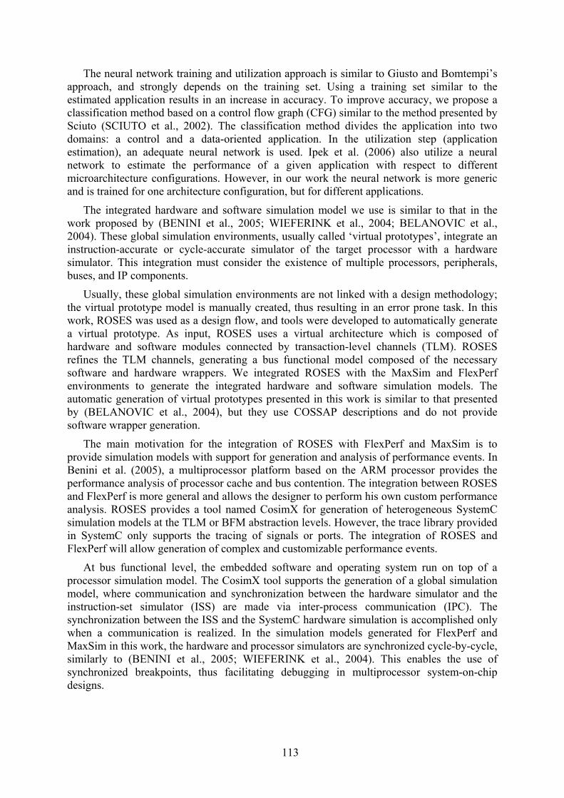
113

The neural network training and utilization approach is similar to Giusto and Bomtempi’s approach, and strongly depends on the training set. Using a training set similar to the estimated application results in an increase in accuracy. To improve accuracy, we propose a classification method based on a control flow graph (CFG) similar to the method presented by Sciuto (SCIUTO et al., 2002). The classification method divides the application into two domains: a control and a data-oriented application. In the utilization step (application estimation), an adequate neural network is used. Ipek et al. (2006) also utilize a neural network to estimate the performance of a given application with respect to different microarchitecture configurations. However, in our work the neural network is more generic and is trained for one architecture configuration, but for different applications.

The integrated hardware and software simulation model we use is similar to that in the work proposed by (BENINI et al., 2005; WIEFERINK et al., 2004; BELANOVIC et al., 2004). These global simulation environments, usually called ‘virtual prototypes’, integrate an instruction-accurate or cycle-accurate simulator of the target processor with a hardware simulator. This integration must consider the existence of multiple processors, peripherals, buses, and IP components.

Usually, these global simulation environments are not linked with a design methodology; the virtual prototype model is manually created, thus resulting in an error prone task. In this work, ROSES was used as a design flow, and tools were developed to automatically generate a virtual prototype. As input, ROSES uses a virtual architecture which is composed of hardware and software modules connected by transaction-level channels (TLM). ROSES refines the TLM channels, generating a bus functional model composed of the necessary software and hardware wrappers. We integrated ROSES with the MaxSim and FlexPerf environments to generate the integrated hardware and software simulation models. The automatic generation of virtual prototypes presented in this work is similar to that presented by (BELANOVIC et al., 2004), but they use COSSAP descriptions and do not provide software wrapper generation.

The main motivation for the integration of ROSES with FlexPerf and MaxSim is to provide simulation models with support for generation and analysis of performance events. In Benini et al. (2005), a multiprocessor platform based on the ARM processor provides the performance analysis of processor cache and bus contention. The integration between ROSES and FlexPerf is more general and allows the designer to perform his own custom performance analysis. ROSES provides a tool named CosimX for generation of heterogeneous SystemC simulation models at the TLM or BFM abstraction levels. However, the trace library provided in SystemC only supports the tracing of signals or ports. The integration of ROSES and FlexPerf will allow generation of complex and customizable performance events.

At bus functional level, the embedded software and operating system run on top of a processor simulation model. The CosimX tool supports the generation of a global simulation model, where communication and synchronization between the hardware simulator and the instruction-set simulator (ISS) are made via inter-process communication (IPC). The synchronization between the ISS and the SystemC hardware simulation is accomplished only when a communication is realized. In the simulation models generated for FlexPerf and MaxSim in this work, the hardware and processor simulators are synchronized cycle-by-cycle, similarly to (BENINI et al., 2005; WIEFERINK et al., 2004). This enables the use of synchronized breakpoints, thus facilitating debugging in multiprocessor system-on-chip designs.

114

3 ANALYTIC SOFTWARE PERFORMANCE ESTIMATION

Currently, SoC designs include one or more processors resulting in an increase of embedded software. The presence of various architectures with different trade-offs concerning factors such as performance and power consumption allows a large design space exploration. Estimation tools for software components are necessary, at a high abstraction level, to determine which is the best processor, in terms of cost, performance, and power, to execute a given application. Analytical methods are proposed to overcome the high cost of obtaining the application execution time using emulation or cycle-accurate simulation.

Performance estimation may be applied in two contexts: worst-case execution time (WCET) evaluation and design space exploration. In WCET evaluation (ENGBLOM; ERMEDAHL; STAPPERT, 2001), one of the main requirements is to guarantee that there will be no underestimation of the execution time of a given application task, since this could cause deleterious effects when using the estimation in the schedulability analysis.

The goal of software performance estimation for design space exploration is to obtain an approximation of the software execution time for a given architecture (GIUSTO et. al, 2001; BONTEMPI; KRUIJTZER, 2002). In this case, as in WCET calculation, precision is also required, although both underestimations and overestimations may be tolerated. In this case, techniques use application profiling, which extracts instructions executed by the application. An analytical or statistical model thus maps the executed instructions to the number of cycles, resulting in low estimation costs.

High-level performance estimation is an interesting alternative, since it may combine low costs for obtaining the performance data with acceptable precision. This allows fast evaluation of different architectural alternatives in the early phases of the design cycle. The main problem in developing an estimation tool is obtaining an accurate performance model that considers advanced architectural features such as pipelines, caches, and branch predictors.

At the functional level, different HW/SW partitions and assignments have to be explored. Software estimation enables rapid processor selection and helps HW/SW partitioning by estimating the SW partition cost. This first estimation is useful in the architecture exploration step (see Figure 3.1).

115


BFM Level

SoC Integration

RTL Level





Processor Selection


Memory mapping

Delay estimation

Scope of this work

Figure 3.1- Performance estimation tool in a global design flow

This chapter is divided as follows. Section 3.1 presents the neural network based performance estimation. Section 3.2 presents the experimental set, and Section 3.3 exposes the experiments and results. Section 3.4 presents a method to classify the application in domains resulting in more accurate results. Finally, Section 3.5 concludes this chapter.

3.1 Neural Network Performance Estimation

In the design of embedded systems, design space exploration can be performed to figure out a solution that satisfies the application requirements, for instance by changing architectural choices and task partitioning. Subsequently, the synthesis process generates the final solution composed of software (operating system, application tasks, drivers), hardware (processors, dedicated IP hardware), and the communication structure. An estimation process can be continuously applied to verify the proposed solution with regard to system requirements.

In embedded software estimation, the use of advanced processors requires accurate and fast estimation tools that consider the performance impact of advanced features, such as caches, branch prediction, and pipelines.

The exact number of cycles required by an application may be obtained using emulation or cycle-accurate simulation. These techniques, however, have an inherent high cost either for the development of the simulation or emulation setting. Table 3.1 presents the simulation and estimation times for 2 different processors, using our proposed method. An x86-based machine (Athlon XP 1500) was used to execute the simulation and estimation tools. A speed-up between 5 and 357 times was achieved compared to cycle-accurate simulation. The estimation time corresponds to the dynamic instruction count and the neural network utilization. The dynamic instruction count uses instruction-accurate simulators to obtain the executed instructions, and its cost is proportional to the application size. An instruction-

116

accurate simulator is faster than a cycle-accurate simulator, since it does not simulate the pipeline and microarchitecture details. Neural network utilization takes only 0.026 seconds with the advantage that its cost is always constant and independent of the application size.

Table 3.1- Comparison between the cycle-accurate simulation and the proposed estimation method

PowerPC FemtoJava

Benchmark Cycle-accurate

(sec)

Estimation

(sec)

Speed-up Cycle-accurate

(sec)

Estimation

(sec)

Speed-up

Quicksort 0.183 0.036 5 5.600 0.266 21

Matrix multiply 25.485 0.134 190 1929.030 5.396 357

Matrix sum 14.904 0.093 160 1300.290 4.676 278

Neural networks have been chosen for performance estimation, since they can generalize their behavior even when the process to be modeled is highly non-linear. In this work, a feed-forward error back-propagation network was used (FREEMAN, 1992), due to its simplicity and adaptation to the non-linear behavior of software performance estimation. Our network is composed of an input layer, a hidden layer, and an output layer. Each layer may have a different number of neurons, and each neuron has a transfer function.

In our case, the input layer has the same number of neurons as instruction types. For the hidden layer, we try to use as few hidden-layer units as possible, because each unit adds a load to the CPU during training and utilization. In our tests, we started the training using in the hidden layer the same number of neurons as in the input layer. Tests showed that the increase of the number of neurons accelerates the training time, but this results in a loss of generalization capability or even does not increase the accuracy.

Figure 3.2 presents the two main steps of our estimation method: training and utilization. In the training phase, a set of samples is presented to the network. In this phase, the inputs are the number of executed instructions for each instruction type (like branches, integer arithmetic, floating point, memory, etc.), while the expected result is the number of cycles consumed by the embedded application. A cycle-accurate simulator is required to extract the number of executed instructions and the cycles consumed by application execution. For each different processor, we have selected a small number of instruction classes that are sufficiently representative of the timing behavior of all instruction types. For better precision, we have also extracted the number of backward and forward branches. All these numbers that relate to instruction count and architectural features could also be obtained statically, by methods already introduced in previous works (ENGBLOM et al., 2001; LI; MALIK, 1995; COLIN; PUAT, 2000).

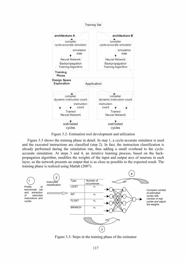
117

TrainingPhase

Design SpaceExploration

simulationdata

instructioncount

compilercycle-accurate simulator

BackpropagationTraining Algorithm

Neural Network

architecture A

TrainedNeural Network

estimatedcycles

compilerdynamic instruction count

simulationdata

instructioncount

compilercycle-accurate simulator

BackpropagationTraining Algorithm

Neural Network

architecture B

TrainedNeural Network

estimatedcycles

compilerdynamic instruction count

Application

Training Set

Figure 3.2- Estimation tool development and utilization

Figure 3.3 shows the training phase in detail. In step 1, a cycle-accurate simulator is used and the executed instructions are classified (step 2). In fact, the instruction classification is already performed during the simulation run, thus adding a small overhead to the cycle-accurate simulation. At steps 3 and 4, an iterative learning process, based on the back-propagation algorithm, modifies the weights of the input and output arcs of neurons in each layer, so the network presents an output that is as close as possible to the expected result. The training phase is realized using Matlab (2007).



LD/ST n1

INT n2

FLOAT n3

BRANCH n4

Compare number of estimated cycles with number of real cycles and adjust the weights

Profile ofbenchmark setand extractionof executedinstructions andcycles

1 2

3

4

Figure 3.3- Steps in the training phase of the estimator

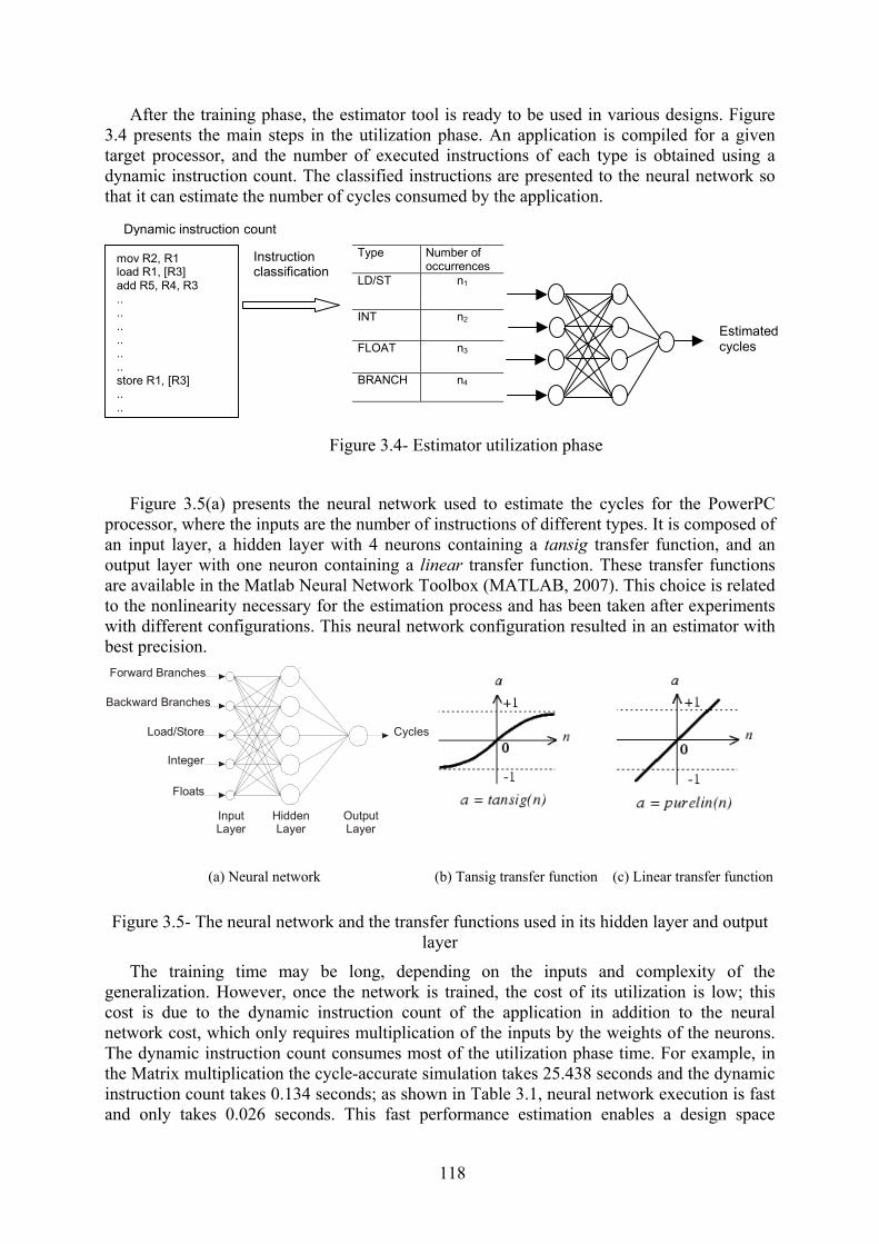
118

After the training phase, the estimator tool is ready to be used in various designs. Figure 3.4 presents the main steps in the utilization phase. An application is compiled for a given target processor, and the number of executed instructions of each type is obtained using a dynamic instruction count. The classified instructions are presented to the neural network so that it can estimate the number of cycles consumed by the application.


LD/ST n1

INT n2

FLOAT n3

BRANCH n4


Estimated cycles

Dynamic instruction count


Figure 3.4- Estimator utilization phase

Figure 3.5(a) presents the neural network used to estimate the cycles for the PowerPC processor, where the inputs are the number of instructions of different types. It is composed of an input layer, a hidden layer with 4 neurons containing a tansig transfer function, and an output layer with one neuron containing a linear transfer function. These transfer functions are available in the Matlab Neural Network Toolbox (MATLAB, 2007). This choice is related to the nonlinearity necessary for the estimation process and has been taken after experiments with different configurations. This neural network configuration resulted in an estimator with best precision.

InputLayer

HiddenLayer

OutputLayer

Forward Branches

Backward Branches

Load/Store

Integer

Floats

Cycles

(a) Neural network (b) Tansig transfer function (c) Linear transfer function

Figure 3.5- The neural network and the transfer functions used in its hidden layer and output layer

The training time may be long, depending on the inputs and complexity of the generalization. However, once the network is trained, the cost of its utilization is low; this cost is due to the dynamic instruction count of the application in addition to the neural network cost, which only requires multiplication of the inputs by the weights of the neurons. The dynamic instruction count consumes most of the utilization phase time. For example, in the Matrix multiplication the cycle-accurate simulation takes 25.438 seconds and the dynamic instruction count takes 0.134 seconds; as shown in Table 3.1, neural network execution is fast and only takes 0.026 seconds. This fast performance estimation enables a design space

119

exploration that would be difficult to accomplish if a cycle-accurate simulator were used, due to the time that it takes to evaluate each new software design. Also, the instruction count can be statically obtained using the methods described in (LI; MALIK, 1995; WOLF; ERNST, 2000).

For each target processor, a different estimator is created. This performance estimation method is adapted for design space exploration in the software domain, for instance by considering various algorithmic alternatives and various ways of partitioning tasks among processors, since architectural modifications in the processors would require a new training process, and thus a long turnaround time.

3.2 Experimental Set

A set of 32 benchmarks (STAPPERT, 2004), listed in Table 3.2, was used for training and testing. Some benchmarks were executed with different input data resulting in a total of 40 samples. This set contained both control-dominated and data-dominated applications. The training process was performed with a mix of applications, and satisfactory estimations were obtained for applications from both domains, thus proving the robustness of the estimator.

Table 3.2- Benchmarks used in experiments Sort and Search

Quicksort, bubble sort, selection sort, sequential search, binary search

Numerical Matrix multiplication, matrix inversion, matrix sum, matrix count, root computation, square root computation, LU decomposition, statistics (mean, variance, standard deviation), Fibonacci calculation, complex number arithmetic operations

Data Processing

FFT, FIR, data compress, DES cryptography, ADPCM (Adaptive Differential Pulse Code Modulation), DCT (Discrete Cosine Transform), CRC (Cyclic Redundancy Check), LMS (least-mean square) algorithm

Synthetic 6 synthetic algorithms

Statecharts Code automatically generated from Statechart descriptions

Figure 3.6 presents the cycle and instruction counts of the benchmarks, considering the PowerPC 750 as the target processor. Benchmarks in the x-axis are ordered by increasing cycle counts. The y-axis is represented in logarithmic scale, which is appropriate for the wide range of applications used to train and test the estimator. The instruction count thus varies from 228 for short code (e.g., device drivers or operating system functions) to 14x106 for huge applications.

120

1,00E+00

1,00E+01

1,00E+02

1,00E+03

1,00E+04

1,00E+05

1,00E+06

1,00E+07

1,00E+08

1 3 5 7 9 11 13 15 17 19 21 23 25 27 29 31 33 35 37 39 41Benchmark

Size

Cycles CountInstruction Count

Figure 3.6- Cycle and instruction count distribution

3.3 Generic Estimator

This section presents the results of the neural network (NN) application with three different architectures: PowerPC, FemtoJava, and Athlon.

3.3.1 PowerPC Generic Estimator The PowerPC 750 processor was used to evaluate the proposed estimation method. It is a

RISC superscalar processor that may complete up to 2 instructions per cycle and contains 6 functional units: a floating-point unit, a branch unit, a system register unit, a load/store unit, and two integer units. A cycle-accurate PowerPC simulator (MICROLIB, 2007) was used to profile each benchmark and to obtain the exact number of cycles consumed by each application. Additionally, the simulator also delivers the number of misses in the data and instruction caches as well as the number of misses in the branch prediction.

In the first phase, a generic estimator was trained using benchmarks 1 to 10 and 30 to 39. They represent a mix of data-dominated and control-dominated applications that have very different sizes, as seen in Figure 3.6. The remaining 21 benchmarks were used to test estimation precision. Benchmarks 40 and 41 are executions of a Crane application with different execution times for the main loop of the control algorithm (MOSER; NEBEL, 1999).

In order to build a first neural network estimator, instructions have been classified into four classes: branches, integer, floating point, and load/store. Table 3.3 presents the results obtained from the experiments and the mean estimation error, standard deviation, maximum underestimation, and maximum overestimation errors. For the neural network, using only four instruction classes, the maximum overestimation is 41.01%, and the maximum underestimation is 20.69%. In the experiments using four instruction classes and considering the training set only, the mean error obtained was 4.81% and the standard deviation was 7.07%. Considering the test set only, we obtained a mean error of 13.30% and a standard deviation of 11.83%. The largest estimation error was obtained with benchmark expint

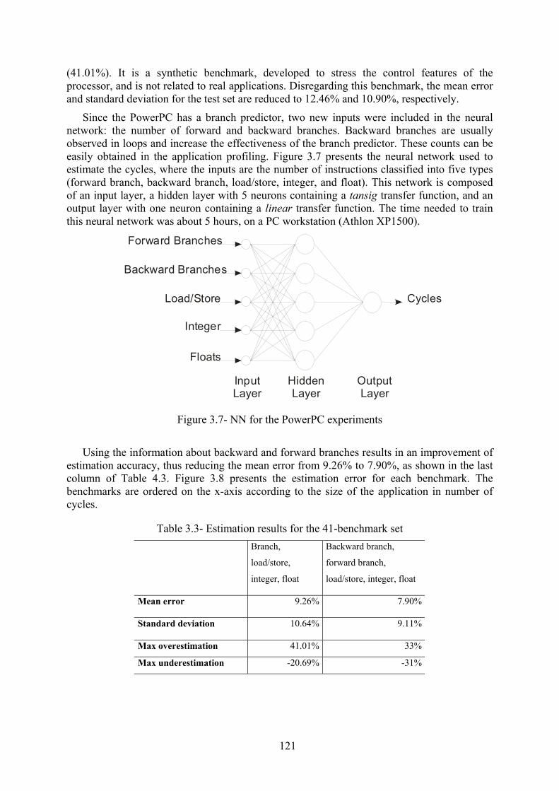
121

(41.01%). It is a synthetic benchmark, developed to stress the control features of the processor, and is not related to real applications. Disregarding this benchmark, the mean error and standard deviation for the test set are reduced to 12.46% and 10.90%, respectively.

Since the PowerPC has a branch predictor, two new inputs were included in the neural network: the number of forward and backward branches. Backward branches are usually observed in loops and increase the effectiveness of the branch predictor. These counts can be easily obtained in the application profiling. Figure 3.7 presents the neural network used to estimate the cycles, where the inputs are the number of instructions classified into five types (forward branch, backward branch, load/store, integer, and float). This network is composed of an input layer, a hidden layer with 5 neurons containing a tansig transfer function, and an output layer with one neuron containing a linear transfer function. The time needed to train this neural network was about 5 hours, on a PC workstation (Athlon XP1500).

InputLayer

HiddenLayer

OutputLayer

Forward Branches

Backward Branches

Load/Store

Integer

Floats

Cycles

Figure 3.7- NN for the PowerPC experiments

Using the information about backward and forward branches results in an improvement of estimation accuracy, thus reducing the mean error from 9.26% to 7.90%, as shown in the last column of Table 4.3. Figure 3.8 presents the estimation error for each benchmark. The benchmarks are ordered on the x-axis according to the size of the application in number of cycles.

Table 3.3- Estimation results for the 41-benchmark set Branch,

load/store,

integer, float

Backward branch,

forward branch,

load/store, integer, float

Mean error 9.26% 7.90%

Standard deviation 10.64% 9.11%

Max overestimation 41.01% 33%

Max underestimation -20.69% -31%

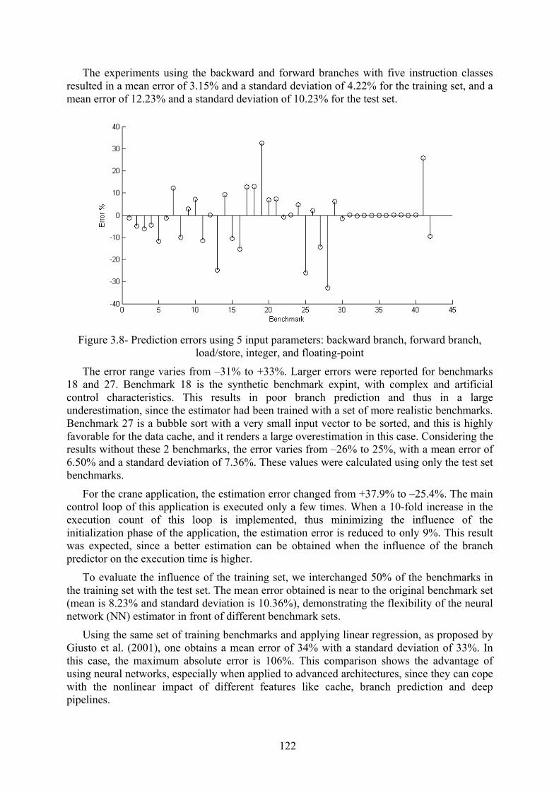
122

The experiments using the backward and forward branches with five instruction classes resulted in a mean error of 3.15% and a standard deviation of 4.22% for the training set, and a mean error of 12.23% and a standard deviation of 10.23% for the test set.

Figure 3.8- Prediction errors using 5 input parameters: backward branch, forward branch,

load/store, integer, and floating-point

The error range varies from –31% to +33%. Larger errors were reported for benchmarks 18 and 27. Benchmark 18 is the synthetic benchmark expint, with complex and artificial control characteristics. This results in poor branch prediction and thus in a large underestimation, since the estimator had been trained with a set of more realistic benchmarks. Benchmark 27 is a bubble sort with a very small input vector to be sorted, and this is highly favorable for the data cache, and it renders a large overestimation in this case. Considering the results without these 2 benchmarks, the error varies from –26% to 25%, with a mean error of 6.50% and a standard deviation of 7.36%. These values were calculated using only the test set benchmarks.

For the crane application, the estimation error changed from +37.9% to –25.4%. The main control loop of this application is executed only a few times. When a 10-fold increase in the execution count of this loop is implemented, thus minimizing the influence of the initialization phase of the application, the estimation error is reduced to only 9%. This result was expected, since a better estimation can be obtained when the influence of the branch predictor on the execution time is higher.

To evaluate the influence of the training set, we interchanged 50% of the benchmarks in the training set with the test set. The mean error obtained is near to the original benchmark set (mean is 8.23% and standard deviation is 10.36%), demonstrating the flexibility of the neural network (NN) estimator in front of different benchmark sets.

Using the same set of training benchmarks and applying linear regression, as proposed by Giusto et al. (2001), one obtains a mean error of 34% with a standard deviation of 33%. In this case, the maximum absolute error is 106%. This comparison shows the advantage of using neural networks, especially when applied to advanced architectures, since they can cope with the nonlinear impact of different features like cache, branch prediction and deep pipelines.

123

We also applied the training method based on the LOO (leave-one-out) technique used by Bontempi et al. (2002), to evaluate the estimator for a same application under different workloads. In this technique, N-1 runs of the same application with different input data are used for training, and one sample is left to evaluate the estimation accuracy, thus creating an application-specific estimator. Table 4 presents the results obtained for the Quicksort and Matrix Multiply algorithms running with 15 different data inputs. The results show that the neural network can highly adapt to estimate the performance of one application in front of new data, resulting in very small prediction errors.

Table 3.4- Estimation performance using the LOO (leave-one-out) training technique Benchmark Mean error

(%) Std deviation

(%) Max error

(%)

Qsort 0.08 0.16 7.18

Matrix multiply 0.12 0.19 7.63

3.3.2 FemtoJava- a Java Microcontroller FemtoJava (ITO; CARRO; JACOBI, 2001) is a stack microcontroller with a Harvard

architecture and Java bytecode execution capability. It has a very simple architecture without a pipeline, branch prediction, or cache. These characteristics make the performance estimation easier, since each instruction type always consumes the same number of cycles. A cycle-accurate simulator (BECK et al., 2003) was used to provide information about the executed instructions and cycle count. For the neural network training, the instructions were divided into four classes; each one requires a constant number of cycles.

In the utilization phase, where a dynamic instruction count is needed, a Java Virtual Machine with trace capabilities (Java, 2007) was used. It allows the execution of the Java application in the host machine, in order to obtain the number of executed instructions of the various classes.

Figure 3.9 presents the errors obtained using a training set with 5 selected benchmarks (1, 2, 11, 12, and 13). We tested different sets of benchmarks and obtained the same error ranges. As expected, errors below 0.001% were achieved due to the simple architecture of the target processor.

Figure 3.9- Prediction errors for the FemtoJava microcontroller

124

In the experiments, the best results were obtained when linear transfer functions were used in each neuron. This result shows that simple architectures can be described precisely with linear functions, but our method can easily cope with this situation because of the flexibility of the neural network. Applying the linear regression approach, as proposed by Giusto et al. (2001), also gives error ranges below 0.1%.

Table 5 presents the estimation time compared to the cycle-accurate simulation time. The estimation time includes both the dynamic instruction count and the classification.

Table 3.5- Estimation speed-up for the FemtoJava processor Benchmark Cycle-accurate

simulation (sec) Estimation (sec) Speed-up

Quicksort 5.60 0.266 21

Matrix multiply 1929.03 5.396 357

Matrix sum 1300.29 4.676 278

3.3.3 Athlon XP Generic Estimator In the practical experiments using the Athlon processor, we used only 27 of the

benchmarks in the entire set of samples, due to the long simulation time and problems with the profile tool. In the first phase, a generic estimator was trained using 16 benchmarks. The remaining 11 benchmarks were used to test the estimation precision. In order to build a first neural network estimator, instructions were classified into five classes: branches, integer, floating point, system, and move. The neural network used in these experiments is composed of an input layer and a hidden layer (each with 5 neurons) as well as an output layer (with one neuron). The input layer uses a purelin transfer function, while the hidden layer uses a tansig transfer function. The output layer also uses a purelin transfer function. The time needed to train this neural network was about one hour, on a PC workstation (Athlon XP1500).

Table 3.6 shows the results of the experiments in terms of mean estimation error, standard deviation, maximum underestimation, and maximum overestimation errors. The mean error for the training set itself was near 0, as expected, while a mean error of 32.33% and a standard deviation of 22.60% were obtained for the estimation of benchmarks from the test set.

Table 3.6- Results with a generic estimator for the Athlon XP Test and training set Test set only

Mean error 13.17% 32.33%

Standard deviation 21.41% 22.60%

Max overestimation 51.15% 51.15%

Max underestimation

-65.46% -65.56%

These less accurate results (compared to PowerPC and FemtoJava) are due to the irregular instruction set and deep pipeline. Using the same set of training benchmarks and applying linear regression, as proposed in (GIUSTO et al., 2001), one obtains a mean error of 49% with a standard deviation of 42%, and a maximum absolute error of 179%.

The high estimation errors obtained with the Athon XP processor suggests the utilization of more inputs or different instruction classification in the neural network. For instance, a mov instruction may consume very different execution cycles, depending on the addressing mode

125

used in the operators (immediate, direct, and indirect). In this case, a sub-classification of mov instructions can result in a more accurate estimation.

3.4 Automatic Domain Classification

In order to improve accuracy, topological information is used to classify the applications and apply domain-specific estimators. We noted that the quality of the prediction was tightly linked to the training set. Indeed, when training set was mostly formed of dataflow benchmarks, the prediction error for a control-dominated application was large. When considering how to further improve the prediction process, the key issue was how to select the correct training set for a certain domain in an automatic way.

The use of static metrics to characterize the application in a given domain was suggested in other works. Sciuto et al. (2002) propose a static method to characterize the application using data-oriented metrics, structural metrics, DSP-oriented metrics, and ASIC-like oriented metrics. The goal is to define the application affinity degree for a given processing element (e.g., a general purpose processor, a DSP processor, or an ASIC implementation) using these metrics.

In our work we used a method based on the application control flow graph (CFG). This topological information is used to classify the applications and to improve the accuracy of estimations.

The classification uses a CFG weight calculation method, based on the number of arcs connecting a given basic block. If a basic block has 2 output arcs, these arcs are assigned a weight of 2, reflecting the cost, in processor performance, of a control statement. The CFG weight is calculated by equation 4.1 and illustrated in Figure 3.10.

__

_nodesnum

arcsweightedweightCFG ∑= (4.1)

In this way, control-dominated applications will have a higher weight value than dataflow applications. The proposed classification method is fast and can be statically implemented without manual intervention.

22

1

1

1

1

1

CFG_weight = = 1.8 5

9

1

22

1 1

1

CFG_weight = = 2 4

8

Figure 3.10- CFG weight method

126

The key idea is that the processor features (e.g., cache, branch prediction) react differently depending on the application domain (control or dataflow), influencing the overall performance. Consequently, the selection and utilization of the most suitable neural network can be implemented without user knowledge. An adapted version of the GNU compiler gcc (GCC Compiler, 2007) was used to dump a file with information concerning the control flow graph (CFG).

3.4.1 PowerPC 750 Domain-specific Estimator The CFG weight criterion has been used to classify the original benchmark set into two

domains, as shown in the Figure 3.11. In domain CF, we have placed applications with high CFG weight and, consequently, with strong control-flow characteristics. Domain DF is composed of applications with low CFG weight, hence presenting dataflow characteristics. A threshold of 1.95 was used to classify the benchmarks; this threshold was defined based on the previous analysis of the benchmark set. The resulting domains are coherent with a classification performed manually, based on the designer’s knowledge. From the original benchmark set, domain CF is composed of 20 applications, and domain DF of 21 applications. From domain CF, we only kept 16 benchmarks, and removed 4 benchmarks (with floating-point instructions) that represent a small set and could be detrimental to neural network generalization. To overcome this restriction, more benchmarks with floating-point instructions should be used, thus improving neural network precision. The domain DF is composed of 10 benchmarks with floating-point instructions, enough for the neural network training.

Training Set

Classification

Domain DF Domain CF

CompilerCycle-accurate simulator

Architecture A

Neural networkBackpropagation training


Architecture B



Architecture A



Architecture B


Application

Classification

Domain DF Domain CF

CompilerDynamic Instruction Count

Architecture A

Trained Neural network


Architecture B



Architecture A



Architecture B


Estimatedcycles

Estimatedcycles

Estimatedcycles

Estimatedcycles

TrainingPhase


or

Training Set

Classification

Domain DF Domain CF


Architecture A



Architecture A



Architecture B



Architecture B



Architecture A



Architecture A



Architecture B



Architecture B


Application

Classification

Domain DF Domain CF


Architecture A



Architecture A



Architecture B



Architecture B



Architecture A



Architecture A



Architecture B



Architecture B


Estimatedcycles

Estimatedcycles

Estimatedcycles

Estimatedcycles

TrainingPhase


or

Figure 3.11- Estimation process with automatic domain classification

Table 3.7 shows the results obtained with the domain-specific estimators. As one can see, their use results in good performance prediction compared to generic estimators. In the DF (dataflow) domain, the mean error decreases from 7.90% in the generic estimator to 6.41% in

127

the domain-specific estimator. The error range is also smaller for the domain-specific estimator; it varies from –32.41% to 25.87%.

In the CF (control flow) domain, the mean error is close to that obtained with the generic estimator. We notice that the benchmark with the largest error (49%) is expint. This is a synthetic benchmark specifically developed to stress control flow features, and it is not related to real applications. If we do not consider the expint, the error range varies from –17.81% to 24.96%, resulting in a mean error of 4.63% and a standard deviation of 3.56% for the test set.

We also analyzed performance prediction using a cross-test. That is, we utilized the CF domain estimator with the DF domain benchmarks, and vice versa. As one can observe in Table 3.7, the use of domain-specific estimators, for applications from an unrelated domain, results in much poorer estimation. This shows the validity of our classification method.

Table 3.7- Estimation results using domain-specific estimators CF domain DF domain Cross-test

(CF vs. DF)

Cross-test

(DF vs. CF)

Mean 7.62% 6.41% 17.65% 55.12%

Std deviation 12.46% 9.45% 12.39% 38.25%

Max overestimation 24.96% 25.87% 42.34% 163.78%

Max underestimation -49.37% -32.41% -28.49% -95.70%

3.4.2 Athlon XP Domain-specific Estimator The CFG weight criterion has been used to classify the original benchmark set, composed

of 27 applications, into two domains. In the original benchmark set, the CF (control-flow) domain is composed of 15 applications and the DF (dataflow) domain is made up of 12 applications. From the former, we kept 14 benchmarks and removed one benchmark with floating point instructions.

Table 3.8 shows the results obtained with the domain-specific estimators. In domain CF, the mean error decreases to 9.9% and the error range varies from 6.44% to -53.82%.

In domain DF (dataflow), the mean error decreases from 13.17%, in the generic estimator, to 6.26%, in the domain-specific estimator. This estimator also yielded a decrease in the error range, which varies here from –29.69% to 26.47%.

Table 3.8- Estimation results using domain-specific estimators for an AthlonXP processor Domain CF Domain DF

Mean 9.9% 6.26%

Std deviation 17.34% 10.86%

Max overestimation 6.44% 26.47%

Max underestimation

-53.82% -29.69%

128

The prediction results for domain CF in the Athlon XP are not as good as those obtained for the PowerPC processor. Indeed, the architecture of the Athlon processor is more complex, resulting in an increase of the prediction error.

Figure 3.12 summarizes the results for the generic estimator and domain-specific estimators, for the PowerPC, Athlon XP, and ADSP processors. They represent three distinct architectures. The first has a RISC architecture, while the second has a CISC architecture composed of nine functional units and other advanced features. The ADSP 218x is a digital signal processor from Analog Devices (ANALOG, 2007). The 218x family shares the same architectural base that is optimized for digital signal processing. It has three functional units (ALU, MAC, and shifter unit) that can operate in parallel. The ADSP is a CISC processor, but the execution cycles of each instruction does not vary much as the Athlon XP, thus increasing the performance estimation accuracy.

In all cases, applying the automatic classification method and generating domain-specific estimators yields gains in estimation precision.

0

2

4

6

8

10

12

14

Athlon PowerPC ADSP

Processors

Mea

n er

ror (

%)

GenericDomain CFDomain DF

Figure 3.12- Comparison between generic and domain-specific estimators for 3 different architectures (Athlon XP, PowerPC, and ADSP)

In general, we obtained the smallest errors in the DF domain, where we have applications with dataflow characteristics. In this type of application, the different processor components achieve the maximum performance (high hit rates in the cache and branch prediction), resulting in a more “predictable” system. On the other hand, the same reductions in error range cannot be obtained for the CF domain, which is composed of control flow applications. Clearly, for the Athlon XP, the error ranges suggest that other parameters are needed to obtain acceptable results with a neural network estimator.

3.5 Conclusions

This work aims at showing the applicability of neural networks use to improve embedded software performance estimation. Our results are more accurate than those previously

129

obtained with linear methods, even when using a more complex architecture. Bontempi and Kruijtzer (BONTEMPI; KRUIJTZER, 2002) report a mean error of 8.8% in the estimations using non-linear estimation methods, for a set of 6 benchmarks, each one executed with 15 different input data sets. They do not report, however, the size of the training and of the test sets. In our case, with a benchmark set composed of 41 benchmarks, we obtained a mean error of 7.90%. Although the direct comparison of the two works cannot be made due to different benchmarks and architectures used in the experiments, the NN estimator obtained similar results even using a more heterogeneous benchmark set.

Ipek (IPEK et al., 2006) also show another application of neural networks for software performance estimation. Differently from our work, they use the neural network to estimate application performance under different architecture configurations (e.g. cache size, cache line size, bus width, etc). The neural network inputs are the architectural parameters and the output is the number of cycles per instruction (CPI).

The rapid and precise performance estimation enables selection of the processor in the architecture exploration phase. Even though the training time is long, neural network utilization is fast. The method requires getting an instruction count, which can be obtained using profiling or static methods. In this work, the dynamic instruction count was used. Results obtained attest that the dynamic instruction count is much faster than cycle-accurate simulation.

In our experiments, 41 benchmarks and real applications from different domains (such as filters, matrix manipulations, sorting algorithms, and an embedded crane control) were used. The PowerPC 750 processor with advanced features (cache, superscalar pipelines, and branch prediction) was used to evaluate predictor precision, and a mean error of 7.90% was obtained.

The control flow graph (CFG) information has been used to classify applications and create domain-specific estimators, increasing estimation accuracy. An adapted version of the GNU-gcc compiler was developed to statically provide the topological information, allowing classification without user intervention. This new method results in a decrease of mean and maximum errors.

130

4 PERFORMANCE ESTIMATION AND ANALYSIS USING AN INTEGRATED HARDWARE AND SOFTWARE SIMULATION MODEL

Multiprocessor System-on-Chip (MPSoC) designs require estimation tools to jointly evaluate hardware and software performance. In a recent study with embedded software designers about development challenges and issues, Krauzer (2007) reports that 31% of designs failed to meet performance expectations, missing performance targets by 50% or more. The first cause indicated by designers was a limited vision of the global system. The second was the limited availability of tracing support. Early design estimation tools are necessary to detect problems as soon as possible in order to avoid or correct design failures.

Traditionally, the mapping between the architecture and application is made in a late stage of the design flow, when a hardware prototype is available. For this reason, a design flow based on the existence of an RTL model can yield unacceptable delays.

The rising complexity of software and architectures makes the implementation of precise performance tools harder. Electronic System-Level (ESL) methodologies have been developed to handle increasing design complexity. The key idea is to start design at an abstract level – that is, higher than RTL – to concurrently develop hardware and software. This chapter proposes the use of virtual prototypes for performance analysis at BFM level (Figure 4.1), providing a simulation model of the architecture before the RTL design.


BFM Level

SoC Integration

RTL Level





Processor Selection



Delay estimation

Scope of thischapter

C code


Simulation model

SW execution time in a cycle accurate simulator

Simulation model(Virtual prototype)



(a)

(b)

(c)

Figure 4.1- Performance estimation tools in MPSoC design

131

Platform-based design (KEUTZER et al., 2000) proposes the use of a fixed platform in order to decrease complexity in the mapping step. With a fixed platform, a set of predefined estimations may be available, making the estimation process more precise.

Component-based design (CESARIO et al., 2002) proposes that system development proceed from a set of predefined HW and SW components. This is a flexible solution, since the architectural solution can be composed of components from several IP vendors. Component-based design must include an environment to integrate these different components and, consequently, to perform interface design.

Performance estimation may be applied at different abstraction levels in the design. The first step is the system specification – where the application is described in a functional way – that does not explicitly describe the hardware and software components. SystemC (2007) and SpecC (2007) are examples of specification languages proposed to deal with the problem of concurrently describing HW and SW.

Estimation performance tools at specification level help the designer determine the partitioning between hardware and software. The increasing importance of the software part and the multiplicity of available options in terms of processor architectures call for tools to help the designer select the most suitable processor.

After the HW/SW partitioning, the “golden” virtual architecture model is created, as shown in Figure 4.2(b). This model is composed of functional components, using transaction-level channels to model the communication. It validates the software and the communication API for system components. The estimation tools can provide information for HW/SW interface design, determining how the TLM channels will be implemented in the architecture.




refinement

SoC Integration

RTL LevelExplicit SW memory mapping

VM1 VM2

VM3 HW

Appl.Tasks

OS

HW wrapper

CPU HW


CPUBFM


Appl.Tasks

OS

HW

Physical Network

CPU

MEM0MEM1

CPU

MEM0MEM1



f1f2

f3f4

HW wrapper

(a)

(b)

(c)

(d)

Figure 4.2- SoC design flow

132

In order to deal with virtual architecture level performance estimation, certain solutions have been developed by the TIMA group. Bouchhima (2005) provides an abstract CPU model that runs the software natively and integrates the hardware components using TLM channels.

The abstract CPU model provides a hardware abstraction layer (Figure 4.3), in such a way that the API calls can be included in the SW code. The CPU abstract model is made up of three main components: the Execution Unit, the Access Unit, and the Data Unit. One or more processing units (PU) form the Execution Unit and are modeled as SystemC threads (SC_THREADS). The Access Unit provides address resolution and synchronization with the memory. The Data Unit models the peripheral access and interrupts. In order to generate interrupts for the software processes (SystemC modules), the Data Unit uses the notify call available in SystemC.

Application SW

HAL API

Nativecompilation

Native binary(library)HAL API

HAL API

Abstract CPUsubsystem

model

HW services

Rest of systemmodel

TLM channel

linking

CPU subsystem

Figure 4.3- Performance estimation using CPU abstract models (adapted from Bouchhima (2005))

The abstract CPU model does not execute the real operating system code, but simulates task serialization (scheduling) and address resolution. This is possible thanks to the Access Unit, which controls memory access conflicts and simulates communication delays.

Software performance is modeled using the traditional annotation method in the code. For each basic block, a delay statement is placed with the number of cycles spent in the execution. The abstract CPU model provides an MPSoC simulation model, where the software is implemented using the target API. Because of the interface with the rest of the system, other hardware components may be used and simulated in an integrated way.

The TLM channels from the virtual architecture have to be refined to obtain the bus functional model (BFM), as shown in Figure 4.2(c). An operating system implements the software communication API. Hardware wrappers adapt the interface between the processor and intellectual property (IP) components in the interconnection structure.

The BFM model is quite different from the RTL model, therefore a SoC integration step is necessary. SoC integration generates software mapping customized for a given memory organization. In each step of the MPSoC design, performance estimation tools verify if the design conforms to the system requirements and, at the same time, provide the information needed for the next design steps, as shown in Figure 4.1.

133

This chapter presents two simulation-based MPSoC performance estimation tools (FlexPerf and MaxSim) for performance analysis at BFM level. These tools are integrated in an MPSoC design tool called ROSES, providing a global performance estimation solution. In order to validate the BFM architecture, the ROSES environment already generates a SystemC simulation model. However, this simulation model does not allow a synchronized cycle-by-cycle execution of hardware and software components. Also, this model provides limited performance analysis resources, present in the SystemC library, such as signal tracing. The main motivation for integrating the FlexPerf and MaxSim environments to ROSES is to provide an extensible performance analysis environment, enabling the performance analysis of MPSoC architectures.

The outline of this chapter is as follows. Section 4.1 describes the FlexPerf environment. Its integration in the ROSES environment is presented in Section 4.2. Section 4.3 presents the MaxSim electronic virtual prototype simulation environment, and Section 4.4 describes its integration with ROSES. Finally, Section 4.5 concludes the chapter.

4.1 FlexPerf

FlexPerf (PAOLI; SANTANA; GALIX, 2004) is a framework for system performance analysis based on the analysis of performance events. FlexPerf is composed of two parts: the instrumentation part, integrated in the simulator, and the profiling part. The designer has access to a pool of off-the-shelf profiling analysis algorithms that can be extended with custom analysis modules. The simulator instrumentation is explicit, so precision depends on the simulator and the instrumentation level.

FlexPerf is organized in three layers of oriented-object software. The first layer is the framework, a collection of objects used to describe all of the SoC resources. This layer is based on a root library “FWlib” and provides mechanisms facilitating object persistency and manipulation, such as object serialization/de-serialization.

The second layer, the analysis layer, is a collection of profiling algorithms. Algorithms depend on the framework, but they do not have any dependency from a given simulator. Consequently, if a simulator is instrumented to generate events using the framework format, a pool of profiling algorithms is available to be used.

The third layer is the configuration layer. It contains all configuration resources for customization of the framework, including a graphical user interface (GUI). In the graphical user interface, shown in Figure 4.4, the information manipulated by FlexPerf is hierarchically classified in three levels corresponding to the system architecture view, the application view, and the analysis view. The GUI supports multiple system instances corresponding to different systems, or different versions, simultaneously. The application view also supports multiple instances of an application description. A session corresponds to a given simulation instance of a system using a specific application and input data set. Performance analyses are realized on the data collected during the simulation session.

The extensibility and modularity of the framework allows the customization of performance analysis resources to user requirements. It includes the creation of new objects, needed for system description, by inheritance of existing ones.

134

Figure 4.4- FlexPerf graphical user interface (PAOLI; SANTANA; GALIX, 2004)

Figure 4.5 presents the four main FlexPerf components: the ProcDesc agent responsible for reading the system architecture view; the ApplDesc agent, which generates the application view; the instrumented simulator; and the data analysis agent modules. These four components, called FlexPerf agents, are integrated in the FlexPerf GUI, but can be used as stand-alone applications.

Whole Description

(CPU + APPLI)

<parser>ProcDesc:Generates the CPUdescription

<disassembler>ApplDesc:Generates the Application description

EventDesc:Event generationsupport

1- ProcessorDescription (xml)

2 - ApplicationInput: (elf prog)

application

Data analysis

Event generation

FlexPerf

InstrumentedSimulator

Instrumentation plug-ins

Whole Description

(CPU + APPLI)

<parser>ProcDesc:Generates the CPUdescription

<disassembler>ApplDesc:Generates the Application description

EventDesc:Event generationsupport

1- ProcessorDescription (xml)

2 - ApplicationInput: (elf prog)

application

Data analysis

Event generation

FlexPerf

InstrumentedSimulator

Instrumentation plug-ins

Figure 4.5- FlexPerf framework components

135

4.1.1 System Architecture View The system architecture view describes all traceable resources of the system. FlexPerf

already contains classes to describe processor pipelines, registers, and memories. For instance, an identifier, a name, and a size, define a register view. As another example, an identifier, a name, a width, a depth, and a minimum-addressable-unit, define a memory component. These classes can be extended to describe user-defined components.

The simulator uses the system description as a database in the performance event generation. In the system description, each element has a unique identifier and signals in which component the event took place.

The system description is stored in an XML format and can be read or generated at run-time using an API included in the FlexPerf framework. The FlexPerf GUI launches the processor description agent that generates or reads the system description from an XML file.

4.1.2 Application View The application view represents the software executing on the processor. A collection of

objects supports the representation of program source files, variables, function and program blocks, as well as program instructions.

A FlexPerf agent is responsible for reading the application in ELF (Executable and Linkable Format) and for generating the application view within the FlexPerf GUI. The application information is extracted using the debug-related data structure provided in ELF format. The software analysis module uses this application information to produce structured application views such as the function call tree.

4.1.3 Analysis View The analysis agent implements the performance analysis algorithms based on the

information generated from the simulation execution. In FlexPerf, a set of analysis agents for processor performance analysis is available and can be extended by the user. FlexPerf provides a set of off-the-shelf analysis algorithms falling into the following categories (PAOLI; SANTANA, GALIX; 2004):

• Hardware resource oriented analyses: access counters (register and memory components); sequence of accesses (read/write) and derived analysis such as data-life duration and event to event latency; instruction sequence extraction.

• Processor instruction oriented analyses: instruction-set usage; NOP rate; branch analysis providing the number of taken, untaken, taken forward, and taken backward branches; parallelism degree (number of instructions executed in parallel).

• Processor micro-oriented analyses: a pipe usage viewer, which provides a time-chart with the pipe behavior; the bubble rate related to unoccupied pipe stages; instructions per cycle.

• Application-oriented analyses: the memory data life duration, memory usage, code coverage, sequence of application events, and function call tree.

The results of these analyses are represented in the FlexPerf GUI visual elements such as pie charts, bar charts, tree charts, and array types. Third party viewers are used to display time-chart results.

136

4.1.4 Simulator Instrumentation FlexPerf has a well-established flow to generate a processor instrumented model described

in LISA (see Figure 4.6). The LISA language (HOFFMANN et al., 2001) is used to describe processor architectures. The language syntax allows a high level of flexibility in the description of the instruction-set of various processors such as SIMD, MIMD, and VLIW-type architectures.

The LISA processor model is instrumented to generate the appropriate events for performance analysis. The complexity of instrumentation depends on model complexity and on the required analysis. For processor models, instrumentation includes the events describing pipe updates, register accesses, and memory accesses. Performance events use a base class called EventRoot. This class contains the base attributes to describe an event and also implements the methods to serialize and deserialize the objects used in event generation and analysis. The EventRoot class can be extended to produce particular information necessary for performance analysis.

The MaxCore tool (ARM, 2007) is employed to generate the software development tool-set, using the LISA description. The software suite includes a cycle-accurate simulation model, a source-level debugger, and a disassembler. MaxCore also generates packages used in the retargeting of third party C compilers.

After simulator generation, the simulator is encapsulated in a FlexPerf agent. The FlexPerf agent implements the base methods to start the simulation and initializes the streams used to send the events to analysis modules.

Simulator and compilergeneration

Processor description in LISA (instrumented)

Simulator(standalone/C++ object)

Compilation

FlexPerf Agent

Simulation Performance Analysis

C Compiler

FlexPerf Integration

Executableapplication

Application

Simulator and compilergeneration

Processor description in LISA (instrumented)

Simulator(standalone/C++ object)

Compilation

FlexPerf Agent

Simulation Performance Analysis

C Compiler

FlexPerf Integration

Executableapplication

Application

Figure 4.6- Simulator instrumentation from LISA processor description

Figure 4.7 presents an example of instrumentation of a SystemC FIFO hardware channel. For each access to the FIFO component, a performance event is generated. The unique identifier represents the component where the event is occurring. This identifier is obtained from the system architecture description. The other parameters are used by analysis agents to generate performance analysis results.

137

void fifo_out::empile_depile(){ .... else { if (CPIMCLK.read()==0 ){ if ((CPIen_n_data==0) && (FIFO_FULL==0)) { tmptail = ((tail+1) % FIFO_depth); fifo[ tail ] = CPIdata_bus.read(); tail = tmptail; #ifdef FW_PROFILER //Component type, Id, cycle, OpType

EventDesc->recordFifoAccess(fw_Component_type, ProcDesc->fifo_outID, sc_simulation_time(), FIFO_IN);

#endif if ((tmptail == head) && (data_defifo==0)) FIFO_FULL = 1; else FIFO_EMPTY = 0; } else status_check(); if ((data_defifo==1) && (FIFO_EMPTY==0)){ .. ..

Figure 4.7- FIFO channel instrumentation example

4.2 ROSES and FlexPerf Integration

The CosimX tool integrates ROSES and FlexPerf, as shown in Figure 4.8. CosimX is a tool for generating heterogeneous simulation models that can be composed of components and interfaces at different abstraction levels. CosimX takes the architecture description from the ROSES design meta-model representation called Colif (CESARIO et al., 2001) and generates the SystemC simulation model. CosimX considers that SystemC models of the hardware interfaces are available in a library of components.

The main motivation for ROSES and FlexPerf integration is the capability to generate more detailed performance events and analysis than are offered by the standard SystemC trace library. The FlexPerf analysis modules are developed for processor-level performance analysis, and their flexibility allows extending the analysis to other system components such as communication resources and peripheral components.

As presented in Figure 4.8, the integration is realized at bus functional level (BFM). At virtual architecture level, the software runs natively and a processor simulation model is not necessary. The SystemC model generated from CosimX adds the FlexPerf interface, enabling support of SystemC module instrumentation and performance event generation.

The bus functional model is generated using ROSES tools for hardware and software interface refinement. At this level, software is compiled to the target processor and runs under an operating system. The SystemC simulation model generated by CosimX uses the instrumented processor simulator generated from a LISA description (see Figure 4.6), resulting in a cycle-accurate model. This integration adds all the software performance analysis capabilities available in FlexPerf to the SystemC simulation. The integration is realized in two parts:

a) A SystemC wrapper is manually implemented, encapsulating the simulator generated from the LISA language.

138

b) The SystemC model generated by CosimX implements the FlexPerf agent interface, making performance event generation possible.

MaxCore produces the processor simulator either as a stand-alone simulator or a library object. This second alternative enables integration of the simulator to any C++ application. The SystemC wrapper uses this library object to encapsulate the simulator and externalizes the BFM signals to SoC simulation.

CosimX supports the generation of simulation models at BFM level using an instruction-set simulator (ISS) connected to SystemC via inter-process communication (IPC). The synchronization between SystemC and the ISS is realized when a communication is made (without a global system clock). The SystemC wrapper implemented in this work fires the processor simulator at each system clock cycle. As a consequence of this, a global synchronized simulation model is obtained.

SystemCsimulation


CosimX +FlexPerf


BFM Level

SoC Integration

RTL Level

ROSESHW/SW interface refinement



Architecture meta-model in Colif

SystemC simulation model

FlexPerf Performance Analysis

FlexPerf performanceevents

Figure 4.8- ROSES and FlexPerf integration flow

The system architecture agent has been changed to automatically generate the FlexPerf system architecture view from the Colif model. This agent is executed when the SystemC simulation is launched. The application view agent is unchanged, since it uses the standard ELF format produced in the compilation step.

Two case studies were conducted to demonstrate the ROSES and FlexPerf integration. The first case study involves a monoprocessor application with FIFO interfaces. Here, FlexPerf integration was only realized at BFM level to validate the extension we proposed for hardware and software integrated analysis. In the second study, a multiprocessor implementation of an MPEG4 encoder was used, and the simulation instrumentation at virtual architecture and bus function model level was realized.

In both cases, at BFM level, software runs in the XiRISC (CAMPI et al., 2001) processor, requiring its inclusion in the ROSES flow. Thus, the XiRISC processor was included in the

139

ASAG (see Section 2.4.2) library, enabling HW interface generation. The operating system generated by ASOG (see Section 2.4.3) was ported and included in the ASOG library, enabling automatic refinement of SW interfaces.

4.2.1 Case Study- FIFO Analysis in a Monoprocessor System This experiment used only one processor. The processor adapter and FIFO (first-in first-

out) interfaces, generated by the ASAG tool, implement the communication co-processor. Figure 4.9 presents the simulation model and the instrumented components.

XiRisc CPU(instrumented)

Processor Adapter

FIFO IN(instrumented)

FIFO OUT(instrumented)

ConsumerProducer

FlexPerf

Data Analysisevents

Figure 4.9- FIFO simulation model

The processor adapter is responsible for controlling the communication interfaces and communication with the processor. Two SystemC models emulating peripheral components (Producer and Consumer) were implemented and used in the simulation.

The purpose of this case study was to demonstrate the integrated performance analysis of hardware and software components. The software is composed of two processes producing and consuming data to/from the interface.

Three analysis modules implement FIFO performance analysis using events generated during the simulation. Each module implements the following analyses concerning FIFO performance:

a) FIFO utilization (which provides the utilization percentage of the FIFO throughout system execution),

b) FIFO operation number and state, and

c) interrupt handler activation interval.

For instance, in Figure 4.10 the buffer utilization module analysis shows the percentage of execution time during which the FIFO buffer stores a given quantity of elements. In this case, the analysis illustrates that the maximum number of elements in the FIFO_OUT buffer was 25 for 0.77% of the execution time. This analysis helps the designer evaluate if the hardware interfaces are well configured for the system application. The analysis also shows the number

140

of INPUT and OUTPUT operations and indicates when the FIFO was in EMPTY or FULL state.

Figure 4.10- FIFO analysis results

In order to accomplish the FIFO performance analysis, the agent module only requires the FIFO identifier number. For systems with many FIFO interfaces, the same performance analysis module can be reused to automatically analyze different instances of the FIFO component.

4.2.2 Case Study- MPEG4 Encoder Multiprocessor System

The second case study features an MPEG4 encoder. We used a flexible architecture presented in (BONACIU et al., 2006), which implements the encoder in two parts. The first is responsible for the motion estimation and DCT encoder, and the second implements the Huffman compression code (VLC). The architecture is flexible and allows the encoder and VLC task parallelization, as shown in Figure 4.11. The architecture includes three hardware components: an Input, a Combiner, and a direct memory access (DMA) component. The Input component divides a frame among the different Encoder processes. The Combiner is responsible for merging the results from the different VLC processes. The last hardware component, the DMA, is responsible for managing transfers among the components.

141

VLC

Fn

CodedImage

VLC Task (SW)

DCT Quant

IDCT

IntraPrediction

ImageReconstruct

MotionEstimation

Fn-1

Encoder Task (SW)

MotionComp.

InputCombiner

Rate control

DMA

DeQuant

Figure 4.11- MPEG4 encoder architecture (BONACIU et al., 2006)

In this case study, we used two processors: one to execute the Encoder task (VPROC0) and another one to execute the VLC (VVLC0) task. Figure 4.12 presents the architecture top-level. VINPUT, VSTORAGE, and VDMA are hardware components. VANTENNA and VSTORAGE blocks are simulation components added to provide the video input and output.

Figure 4.12- MPEG4 encoder top-level architecture

The ROSES hardware interface refinement generates the CPU subsystem for each software component, based on an architecture template. The software interface refinement generates the application-specific operating system, based on the communication API. Figure 4.13 presents the CPU subsystem of the VPROC0 component. The XiRISC processor executes the software. The memory control component (CMIMemCtrl) implements a double-bank memory, enabling parallel processing and transfer of the next frame to the memory.

The processing flow is as follows: VINPUT loads the image frame into memory and signals the VDMA that this has been done. The processor VPROC0 changes the bank memory, and VINPUT continues to load the next frame into memory. For each macroblock processed by VPROC0, it sends the data to the VVLC0 process. After frame encoding, the

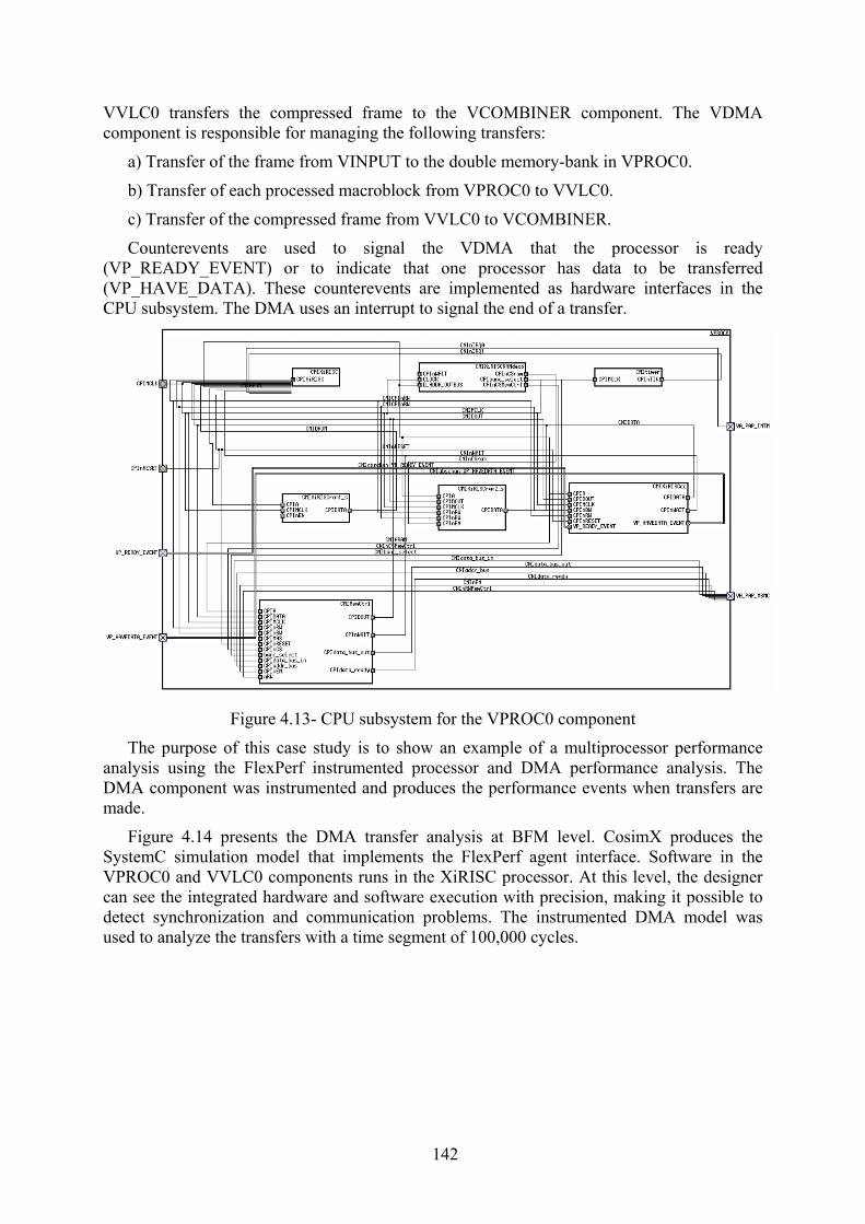
142

VVLC0 transfers the compressed frame to the VCOMBINER component. The VDMA component is responsible for managing the following transfers:

a) Transfer of the frame from VINPUT to the double memory-bank in VPROC0.

b) Transfer of each processed macroblock from VPROC0 to VVLC0.

c) Transfer of the compressed frame from VVLC0 to VCOMBINER.

Counterevents are used to signal the VDMA that the processor is ready (VP_READY_EVENT) or to indicate that one processor has data to be transferred (VP_HAVE_DATA). These counterevents are implemented as hardware interfaces in the CPU subsystem. The DMA uses an interrupt to signal the end of a transfer.

Figure 4.13- CPU subsystem for the VPROC0 component

The purpose of this case study is to show an example of a multiprocessor performance analysis using the FlexPerf instrumented processor and DMA performance analysis. The DMA component was instrumented and produces the performance events when transfers are made.

Figure 4.14 presents the DMA transfer analysis at BFM level. CosimX produces the SystemC simulation model that implements the FlexPerf agent interface. Software in the VPROC0 and VVLC0 components runs in the XiRISC processor. At this level, the designer can see the integrated hardware and software execution with precision, making it possible to detect synchronization and communication problems. The instrumented DMA model was used to analyze the transfers with a time segment of 100,000 cycles.

143

Figure 4.14- DMA transfer analysis at BFM Level

The number of transfers for each time segment indicates low utilization of the DMA. At every 100.000 cycles, the maximum number of transfers managed by the DMA is below 4200. Considering that each transfer takes one cycle, this gives a maximum activity of 4% of the execution time.

4.3 MaxSim ESL Design

MaxSim (ARM, 2007) is an environment for virtual prototype modeling and simulation based on SystemC. The designer can build a virtual prototype, assembling the system by drawing from a component library. This component library is composed of processors, buses, memories, and peripheral controllers, among others. The library can be extended with custom components described by the designer.

The computational model of the MaxSim components is based on a cycle-based engine. For this kind of component, the behavior is evaluated only in the clock edges. Two methods describe the component behavior: communicate and update. In the communicate method, all communications between the components are performed, whereas in the update method the completed communications are committed in the shared resources. This modeling approach leads to high simulation speeds, enabling rapid validation of the architecture.

In MaxSim, an interface called MxSI is used to interconnect the components. MaxSim also provides two other interfaces (Figure 4.15). The MxDI interface allows a debugger connection to the component and is mainly used in processor components. The MxPI interface is used to generate performance events, enabling component profiling.

144

Figure 4.15- MaxSim component interfaces (ARM, 2007)

MaxSim components use two kinds of ports: signal and transaction. The signal-based connection uses the same semantic as RTL models. In a transaction-based connection, operations are described by two methods: read and write. Read and write operations are composed of three parameters: address, value, and control. These methods always return a flag that signals the access state (committed or resource not available). This is useful for modeling conflicts or operations that take more than one cycle, such as a memory access. Also, the control parameter encapsulates other information specific to the communication protocol. A component may use these two kinds of interfaces. As an example, Figure 4.16 shows the ARM9 processor interface, composed of signal-level interfaces (fiq, irq, reset) and transaction-level interfaces (ahb, dtcm, itcm), used to connect the processor with memory modules.

TLM Interfaces: Address map defined in the portsTLM Interfaces: Address map defined in the ports

Figure 4.16- MaxSim model example

The interconnection among the components uses explicit structures like bus components (see Figure 4.16). This enables the mapping of memory modules and IO components, defining the address space for software development. MaxSim also supports event-based SystemC modules. This can be accomplished by instantiating the SystemC component inside a MaxSim component. An interface adapter (shown in Figure 4.17) between the SystemC ports and MaxSim ports is necessary.

145

MaxSim Component

SystemC component

MxSI InterfaceSystemCInterface

Interfaceadapter

Interface adapter

Figure 4.17- MaxSim SystemC wrapper

For basic SystemC signal-level ports sc_in and sc_out, we have implemented generic adapters, thus facilitating the integration of SystemC component into MaxSim. These adapters are responsible for converting the SystemC signal-level interface into the MaxSim MxSI interface, as shown in Figure 4.18. MaxSim exchanges values as integers and the adapter makes the type conversion when necessary. This is useful to integrate RTL models, available in SystemC, into MaxSim simulations.

MaxSim ComponentSystemC module

sc_signal

interfaceadapter

outp->driveSignal(X)

MaxSim Component

MxSignalSlave MxSignalMaster

driveSignal()

Adapts the driveSignal() to the

SystemCsignal

sc_in

sc_out

Adapts a write from SystemC portto a driveSignal() in the MxSignalMaster port

driveSignal()

Figure 4.18- SystemC encapsulation in MaxSim components

4.4 ROSES Integration

As shown in Figure 4.19, the ROSES and MaxSim integration is accomplished at BFM level, following the refinement of hardware and software interfaces. A MaxSim simulation model is generated from the COLIF design meta-model. A MaxSim component encapsulates a SystemC component using the interface adapters. The MaxSim component is automatically generated. To do so, the following information is required:

• port name,

• port type, and

• port direction.

The Colif model provides these port characteristics, automating the generation of the MaxSim components and its inclusion in MaxLib.

146

MaxSimsimulation


Colif2MaxSim


BFM Level

SoC Integration

RTL Level

ROSESHW/SW interface refinement



Architecture meta-model in Colif

MaxSim Virtual Prototype

MaxSim Performance Analysis

Performanceevents

Figure 4.19- MaxSim integration in the ROSES design flow

The hierarchical COLIF model is preserved in MaxSim. Hierarchical components are described in MaxSim using a text format. They contain the subsystem components and their interconnections. This kind of component is also automatically generated from the COLIF model.

MaxSim and ROSES integration enables the automatic virtual prototype generation. The virtual prototype generated from the ROSES architecture description provides all performance analysis resources available in MaxSim environment, such as software debuggers, software execution timeline, and communication analysis. These analyses performance resources are not available in the previous SystemC model generated by CosimX tool, provided by ROSES.

In Chapter 6, a case study of an MPEG4 encoder is elaborated in order to evaluate a high performance estimation tool based on neural networks and the integration of MaxSim and ROSES. The case study will illustrate the resources of the MaxSim virtual prototype that are used to analyze the performance of MPSoC designs.

4.5 Conclusions

This chapter presented two different paths for system performance analysis at bus functional model level. First, a processor-centric approach (FlexPerf) was extended and integrated to ROSES, allowing integrated hardware and software performance analysis. Second, a virtual prototype modeling and simulation tool was integrated to the ROSES environment.

The FlexPerf environment was extended to allow integrated hardware and software performance analysis. We generated a SystemC model, where wrappers are used to encapsulate the instrumented processor simulator generated from the LISA language. This provides an MPSoC global simulation model allowing a synchronized simulation of the hardware and software components. The instrumentation support provided by FlexPerf adds

147

more complex analysis resources than are available in SystemC, where the profile only supports the tracing of ports and signals.

ROSES and FlexPerf integration was evaluated in two case studies: one involving a simple FIFO interface and the other one an MPEG4 encoder. The analysis modules were extended to provide FIFO and DMA performance analysis. FlexPerf’s flexibility and modularity were exploited to extend existing analysis capabilities and to develop new ones.

On the other hand, a virtual prototype tool such as MaxSim seem promising. The support for SystemC custom modules is an important feature, since the MPSoC design always involves IP components that will not be available in the standard library. The SystemC support was used to integrate MaxSim to the ROSES design, with the automatic generation of the MaxSim simulation model from the COLIF design meta-model. The automatic virtual prototype generation enables the designer to spend time on performance analysis instead of on simulation model implementation.

In the prior simulation model generated by CosimX, the ISS was connected with the SystemC simulation using inter-process communication (IPC), and the synchronization was made only at each communication. The integration of FlexPerf and MaxSim to the ROSES environment enabled the generation of a global simulation where the software part (processor simulator) is synchronized cycle-by-cycle with the hardware modules (SystemC).

The simulation model generated in this work is similar to that in (BENINI et al., 2005; WIEFERINK et al., 2004), where a SystemC wrapper encapsulates a processor simulator and is then integrated with the rest of the SystemC simulation. These environments provide certain fixed processors and bus performance analysis resources, but there is no clear way to customize them. In this work, the FlexPerf framework allows instrumentation and performance analysis of SystemC simulation models to be accomplished in an easy and flexible way. Moreover, framework modularity enables reuse of developed analyses for future designs. FlexPerf’s off-the-shelf resources for instrumentation and performance analysis of stand-alone processors were extended to support SystemC MPSoC simulation models, providing a systematic path to integrated performance analysis. ROSES and MaxSim integration also allows the construction of a global simulation model with performance analysis capabilities. The graphical interface provides a comprehensive MPSoC simulation and validation tool allowing synchronized breakpoints in software code, connections, and hardware registers.

Virtual prototype environments, such as ConvergenSC (Coware, 2007), Synopsys System Studio (Synopsys, 2007), and MaxSim (ARM, 2007) propose that architecture design starts from the virtual prototype. In the ROSES environment, design starts at the virtual architecture level and the automatic generation of the virtual prototype accelerates design and decreases error. Furthermore, such environments do not support the generation of software wrappers, as provided in the ROSES environment.

The proposed method makes explicit instrumentation necessary, and, consequently, access to the component code is also required. Considering that the ROSES environment uses a component-based approach, the components in the library could be instrumented beforehand. This idea could be extended to SystemC channels, which can be pre-instrumented to automatically generate performance events.

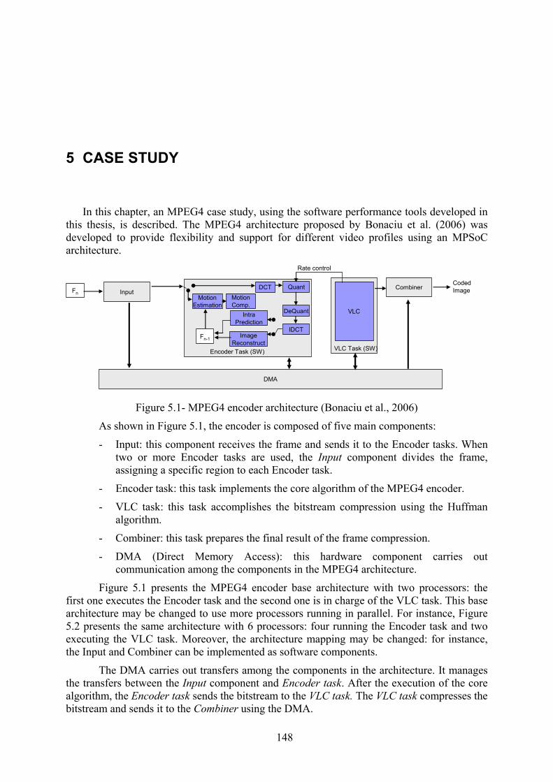
148

5 CASE STUDY

In this chapter, an MPEG4 case study, using the software performance tools developed in this thesis, is described. The MPEG4 architecture proposed by Bonaciu et al. (2006) was developed to provide flexibility and support for different video profiles using an MPSoC architecture.

VLC

Fn

CodedImage

VLC Task (SW)

DCT Quant

IDCT

IntraPrediction

ImageReconstruct

MotionEstimation

Fn-1

Encoder Task (SW)

MotionComp.

InputCombiner

Rate control

DMA

DeQuant

Figure 5.1- MPEG4 encoder architecture (Bonaciu et al., 2006)

As shown in Figure 5.1, the encoder is composed of five main components:

- Input: this component receives the frame and sends it to the Encoder tasks. When two or more Encoder tasks are used, the Input component divides the frame, assigning a specific region to each Encoder task.

- Encoder task: this task implements the core algorithm of the MPEG4 encoder.

- VLC task: this task accomplishes the bitstream compression using the Huffman algorithm.

- Combiner: this task prepares the final result of the frame compression.

- DMA (Direct Memory Access): this hardware component carries out communication among the components in the MPEG4 architecture.

Figure 5.1 presents the MPEG4 encoder base architecture with two processors: the first one executes the Encoder task and the second one is in charge of the VLC task. This base architecture may be changed to use more processors running in parallel. For instance, Figure 5.2 presents the same architecture with 6 processors: four running the Encoder task and two executing the VLC task. Moreover, the architecture mapping may be changed: for instance, the Input and Combiner can be implemented as software components.

The DMA carries out transfers among the components in the architecture. It manages the transfers between the Input component and Encoder task. After the execution of the core algorithm, the Encoder task sends the bitstream to the VLC task. The VLC task compresses the bitstream and sends it to the Combiner using the DMA.

149

While one frame is being processed, the next frame is loaded into the Encoder processor by the Input component. This concurrent access to the memory in the Encoder processor is accomplished using a double-bank memory.

VLC

Fn

CodedImage

Rate control

VLC Task (SW)

DCT Quant

DeQuant

IDCT

IntraPrediction

ImageReconstruct

MotionEstimation

Fn-1

Encoder Task (SW)

MotionComp.

DCT Quant

IDCT

IntraPrediction

ImageReconstruct

MotionEstimation

Fn-1

Encoder Task (SW)

MotionComp.

Input

Combiner

Rate control

DMA

DeQuant

DCT Quant

DeQuant

IDCT

IntraPrediction

ImageReconstruct

MotionEstimation

Fn-1

Encoder Task (SW)

MotionComp.

DCT Quant

DeQuant

IDCT

IntraPrediction

ImageReconstruct

MotionEstimation

Fn-1

Encoder Task (SW)

MotionComp.

DCT Quant

DeQuant

IDCT

IntraPrediction

ImageReconstruct

MotionEstimation

Fn-1

Encoder Task (SW)

MotionComp.

DCT Quant

DeQuant

IDCT

IntraPrediction

ImageReconstruct

MotionEstimation

Fn-1

Encoder Task (SW)

MotionComp.

VLC

VLC Task (SW)

Figure 5.2- MPEG4 architecture with four Encoder tasks and two VLC tasks

In this chapter, we will evaluate the proposed estimation methods, using the MPEG4 encoder architecture shown in Figure 5.1, with one processor executing the Encoder task and another one executing the VLC task. The Input, Combiner, and DMA components are implemented in hardware. The main purposes of this case study is to estimate the performance requirements of the Encoder and VLC tasks and to explore the processors that could be used to execute these tasks.

5.1 Performance Estimation and Analysis Flow

In the MPEG4 encoder analysis, the design flow shown in Figure 5.3 will be followed. From the system specification in C, software performance will be estimated using a high-level estimator. In our case study, the Encoder and VLC software components are the targets for software performance analysis.

150

This first estimation step is carried out to guide processor selection for the software components. The neural network estimator developed in this work is utilized for fast estimation of software performance to select a suitable processor.

Design space exploration results in a virtual architecture with explicit hardware and software mapping. In this work, the virtual architecture will not be used for performance estimation and analysis purposes. In other works by the SLS group, this model is employed to obtain the performance estimation, using an abstract CPU model (BOUCHHIMA et al., 2005).

Following processor selection, the virtual architecture is used in the ROSES environment to refine the hardware and software interfaces. Interface refinement depends on the target architecture selected in the exploration step, because certain parts of operating systems and hardware adapters are architecture-specific components. After the HW and SW refinement, a bus functional model (BFM) is generated.

In order to analyze the performance of the BFM model, a virtual prototype is automatically generated using the ROSES architecture description. For generation of the virtual prototype, we consider that the HW components are available as SystemC cycle-accurate models. The software is organized in tasks and runs on an operating system tailored to the application. The virtual prototype will be generated in the MaxSim environment described in Section 5.4.




refinement

VM1 VM2

VM3 HW

Appl.Tasks

OS

HW wrapper

CPU HW


CPU


Appl.Tasks

OS



f1f2

f3f4 Processor



(a)

(b)

Figure 5.3- MPSoC performance estimation design flow

5.2 High-level Estimation

In the first step, we use neural networks to estimate software performance. In the case study, the Encoder and VLC tasks are evaluated. Despite the simplification of the architecture, with only two processors, processor selection and high-level performance estimation still are important aspects of architecture exploration.

In the experiments, two processors are evaluated: the ARM946 and the PowerPC750. Both processors have advanced features commonly found in actual embedded processors,

151

such as pipelines and caches. These features have a non-linear impact on software execution time making performance estimation difficult.

In order to estimate the performance of the Encoder and VLC tasks, these are implemented without the system calls used for communication and synchronization.

The neural network estimator employed for the high-level estimation uses a training approach. This means that a training set is needed to calibrate the estimator. In order to train the ARM946 and PowerPC750 estimators, a set of 41 benchmarks was used to test their accuracy.

Figure 5.4 presents the neural network used to estimate the application cycle count for the ARM946 processor, where the inputs are the number of instructions of different types. This neural network is composed of an input layer, a hidden layer with 5 neurons containing a tansig transfer function, and an output layer with one neuron containing a linear transfer function. These transfer functions are available in the Matlab Neural Network Toolbox (Matlab, 2007). We have selected a small number of instruction classes that are sufficiently representative of the timing behavior of all instruction types (forward branch, backward branch, load/store, multiple load/store, and ALU).

InputLayer

HiddenLayer

OutputLayer

Forward Branches

Backward Branches

Load/Store

Multiple Load/Store

ALU

Cycles

Figure 5.4- NN performance estimation for the ARM9 processor

For each processor, a set of instruction types is chosen to best represent the application performance. In the case of the PowerPC750, the instruction types are forward branch, backward branch, load/store, integer, and float (see Figure 5.5).

For neural network training, a cycle-accurate simulator is required to extract the number of executed instructions and the total number of cycles consumed. For the ARM946 processor, a cycle-accurate simulator provided in the MaxSim environment was used to profile the benchmark set (ARM, 2007). For the PowerPC750, a cycle-accurate simulator from Microlib (2007) was used.

InputLayer

HiddenLayer

OutputLayer

Forward Branches

Backward Branches

Load/Store

Integer

Floats

Cycles

Figure 5.5- NN performance estimation for the PowerPC750 processor

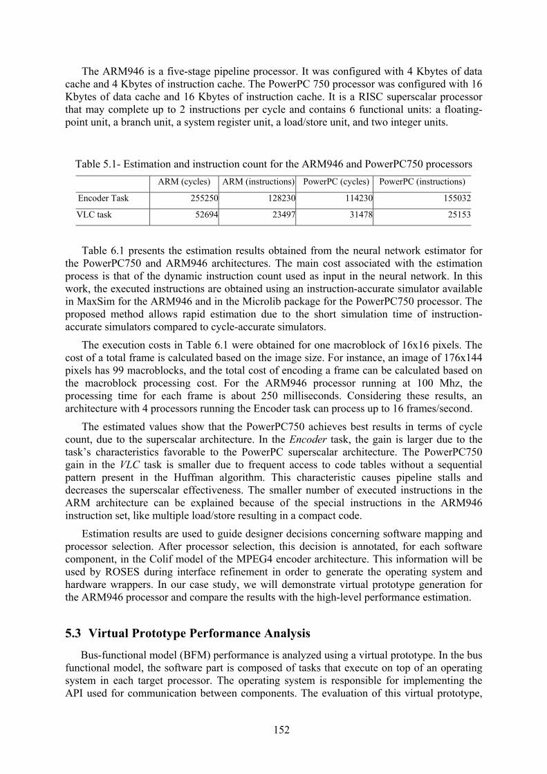
152

The ARM946 is a five-stage pipeline processor. It was configured with 4 Kbytes of data cache and 4 Kbytes of instruction cache. The PowerPC 750 processor was configured with 16 Kbytes of data cache and 16 Kbytes of instruction cache. It is a RISC superscalar processor that may complete up to 2 instructions per cycle and contains 6 functional units: a floating-point unit, a branch unit, a system register unit, a load/store unit, and two integer units.

Table 5.1- Estimation and instruction count for the ARM946 and PowerPC750 processors ARM (cycles) ARM (instructions) PowerPC (cycles) PowerPC (instructions)

Encoder Task 255250 128230 114230 155032

VLC task 52694 23497 31478 25153

Table 6.1 presents the estimation results obtained from the neural network estimator for the PowerPC750 and ARM946 architectures. The main cost associated with the estimation process is that of the dynamic instruction count used as input in the neural network. In this work, the executed instructions are obtained using an instruction-accurate simulator available in MaxSim for the ARM946 and in the Microlib package for the PowerPC750 processor. The proposed method allows rapid estimation due to the short simulation time of instruction-accurate simulators compared to cycle-accurate simulators.

The execution costs in Table 6.1 were obtained for one macroblock of 16x16 pixels. The cost of a total frame is calculated based on the image size. For instance, an image of 176x144 pixels has 99 macroblocks, and the total cost of encoding a frame can be calculated based on the macroblock processing cost. For the ARM946 processor running at 100 Mhz, the processing time for each frame is about 250 milliseconds. Considering these results, an architecture with 4 processors running the Encoder task can process up to 16 frames/second.

The estimated values show that the PowerPC750 achieves best results in terms of cycle count, due to the superscalar architecture. In the Encoder task, the gain is larger due to the task’s characteristics favorable to the PowerPC superscalar architecture. The PowerPC750 gain in the VLC task is smaller due to frequent access to code tables without a sequential pattern present in the Huffman algorithm. This characteristic causes pipeline stalls and decreases the superscalar effectiveness. The smaller number of executed instructions in the ARM architecture can be explained because of the special instructions in the ARM946 instruction set, like multiple load/store resulting in a compact code.

Estimation results are used to guide designer decisions concerning software mapping and processor selection. After processor selection, this decision is annotated, for each software component, in the Colif model of the MPEG4 encoder architecture. This information will be used by ROSES during interface refinement in order to generate the operating system and hardware wrappers. In our case study, we will demonstrate virtual prototype generation for the ARM946 processor and compare the results with the high-level performance estimation.

5.3 Virtual Prototype Performance Analysis

Bus-functional model (BFM) performance is analyzed using a virtual prototype. In the bus functional model, the software part is composed of tasks that execute on top of an operating system in each target processor. The operating system is responsible for implementing the API used for communication between components. The evaluation of this virtual prototype,

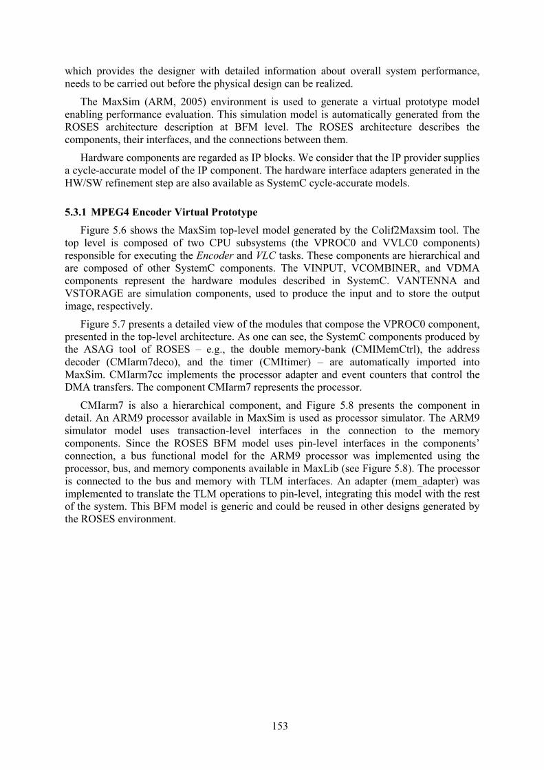
153

which provides the designer with detailed information about overall system performance, needs to be carried out before the physical design can be realized.

The MaxSim (ARM, 2005) environment is used to generate a virtual prototype model enabling performance evaluation. This simulation model is automatically generated from the ROSES architecture description at BFM level. The ROSES architecture describes the components, their interfaces, and the connections between them.

Hardware components are regarded as IP blocks. We consider that the IP provider supplies a cycle-accurate model of the IP component. The hardware interface adapters generated in the HW/SW refinement step are also available as SystemC cycle-accurate models.

5.3.1 MPEG4 Encoder Virtual Prototype Figure 5.6 shows the MaxSim top-level model generated by the Colif2Maxsim tool. The

top level is composed of two CPU subsystems (the VPROC0 and VVLC0 components) responsible for executing the Encoder and VLC tasks. These components are hierarchical and are composed of other SystemC components. The VINPUT, VCOMBINER, and VDMA components represent the hardware modules described in SystemC. VANTENNA and VSTORAGE are simulation components, used to produce the input and to store the output image, respectively.

Figure 5.7 presents a detailed view of the modules that compose the VPROC0 component, presented in the top-level architecture. As one can see, the SystemC components produced by the ASAG tool of ROSES – e.g., the double memory-bank (CMIMemCtrl), the address decoder (CMIarm7deco), and the timer (CMItimer) – are automatically imported into MaxSim. CMIarm7cc implements the processor adapter and event counters that control the DMA transfers. The component CMIarm7 represents the processor.

CMIarm7 is also a hierarchical component, and Figure 5.8 presents the component in detail. An ARM9 processor available in MaxSim is used as processor simulator. The ARM9 simulator model uses transaction-level interfaces in the connection to the memory components. Since the ROSES BFM model uses pin-level interfaces in the components’ connection, a bus functional model for the ARM9 processor was implemented using the processor, bus, and memory components available in MaxLib (see Figure 5.8). The processor is connected to the bus and memory with TLM interfaces. An adapter (mem_adapter) was implemented to translate the TLM operations to pin-level, integrating this model with the rest of the system. This BFM model is generic and could be reused in other designs generated by the ROSES environment.

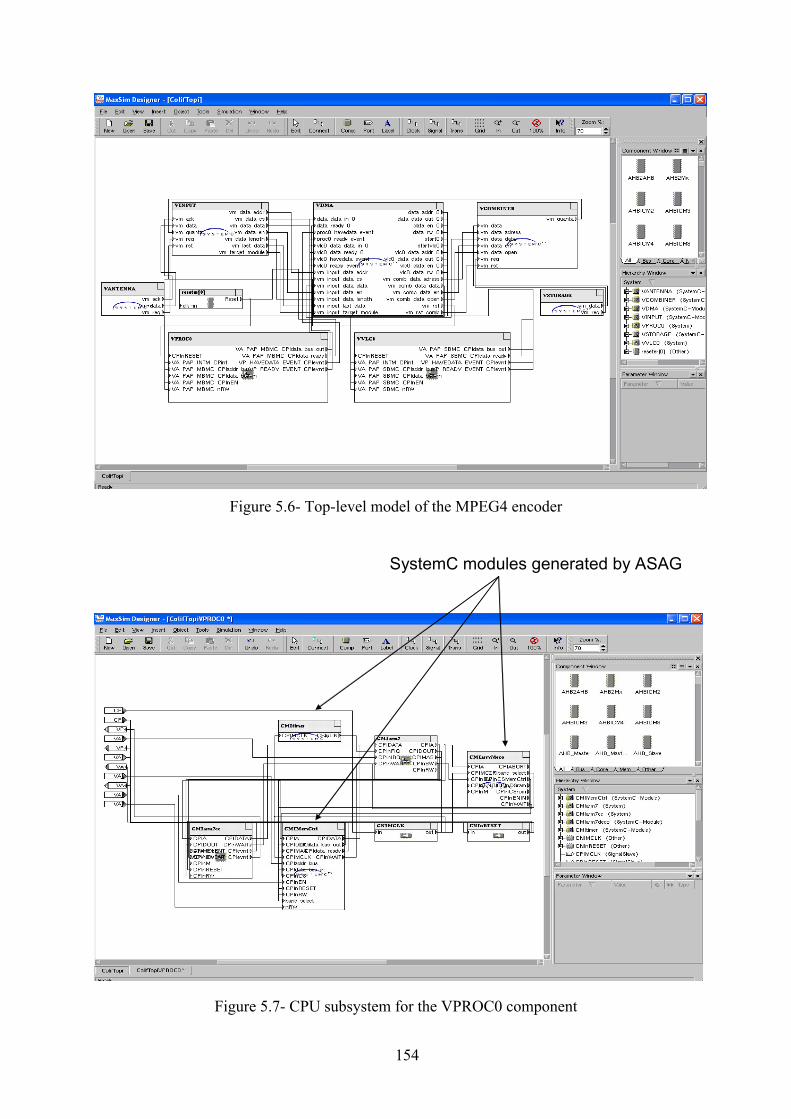
154

Figure 5.6- Top-level model of the MPEG4 encoder


Figure 5.7- CPU subsystem for the VPROC0 component

155

Figure 5.8- BFM model of the ARM9 processor in MaxSim

Figure 5.9 shows the simulation’s initial screen. The MPEG4 encoder implemented in this case study uses two processors, and the binary code containing the application and OS is provided in the simulation initialization.

MaxSim provides global validation support, enabling the use of breakpoints in software code, registers, memory position, and connections. Figure 5.10 presents the software debugging capabilities with the assembler code for the VVLC0 processor. Software debugging is available for all processor components. The global simulation provides a suitable tool for debugging concurrent applications executing in different processors.

Figure 5.9- MaxSim Explorer initial screen

156

Figure 5.10- Software debugging support in MaxSim

Figure 5.11 presents the timeline for software execution in the VPROC0 component. This analysis view enables the designer to find optimization points and analyze the cost of each function within the overall software execution.

Performance analysis resources, such as assembler code debugging, register view, and software execution timeline, come already built-in in library components. Furthermore, for the processor at cycle-accurate level, the model also provides cache performance analysis.

Figure 5.12 shows the communication analysis feature available for bus components. By conducting this analysis, one can verify communication performance, detecting bottlenecks between the processor and memory. This analysis shows the number of accumulated operations in the bus, classified by type (e.g., read, write, request and grant), for each time segment. In the example illustrated by Figure 5.12, the segment size is 10 cycles.

157

Figure 5.11- Software timeline execution

In MaxSim, user components can be instrumented to produce performance events. This resource is provided by the MxPI interface available in the MaxSim components. This interface produces a stream where events are written. Visualization is always accomplished through XY graphics.

Figure 5.13 shows the DMA transfer analysis. The graph plots the number of transfers handled by the DMA, as a function of time. This chart also uses the notion of time segment and, in this example, a size of 100,000 cycles was used. Here, black bars represent transfers between VINPUT and VPROC0, whereas white bars represent transfers between VPROC0 and VVLC0.

158

Figure 5.12- Bus transfer analysis

Figure 5.13- DMA transfer analysis

The comparison of the performance estimation from the neural network to that obtained with the virtual prototype is shown in Table 5.2. For the PowerPC750 processor, a SystemC cycle-accurate simulation model was used, but without the operating system and hardware interfaces. Although this simplification limits the system performance analysis, the cycle-accurate model enables the verification of the NN estimator accuracy. For the ARM946 processor, the estimation error was 4.26% for the Encoder task and -8.29% for the VLC task. For the PowerPC750 processor, an error of 24.8% in the Encoder task was obtained. This was expected, however, given that the PowerPC750 processor is more complex, making estimation more difficult.

If we apply linear regression for performance estimation, as proposed by Giusto et al. (2001), the estimation errors obtained for the ARM946 architecture were 60.25% and 58.66%, for the Encoder and VLC tasks, respectively. For the PowerPC750 processor, we observed

159

that linear regression also revealed higher estimation errors (87% for the Encoder task and 44.42% for the VLC task). This demonstrates the neural network’s flexibility and capability for non-linear prediction.

Table 5.2- High-level performance estimation (in cycles) compared to the cycle-accurate virtual prototype

ARM946 PowerPC750 Estimated Cycle-accurate Error Estimated Cycle-accurate Error Encoder Task 255250 266630 4.26% 114230 151960 24.8%

VLC Task 52694 48659 -8.29% 31478 31064 1.33%

Table 5.3 presents estimation and virtual prototype execution times for macroblock processing. As indicated, a speed-up between 6.5 and 22 times was achieved with the neural network with regard to the virtual prototype. Considering the increasing size of embedded software code, neural network estimation enables rapid evaluation of various solutions without high simulation costs. In turn, the virtual prototype enables global analysis of hardware and software components. This allows detailed system performance analysis and confirmation of numbers estimated at higher abstraction levels.

Table 5.3- Estimation and cycle-accurate virtual prototype simulation times ARM946 PowerPC750

Cycle-accurate

(s) Estimation (s) Speedup Cycle-accurate

(s) Estimation (s) Speedup

Encoder Task 5.5 0.3 22.0 4.3 0.3 14.3VLC Task 3.0 0.2 14.3 1.4 0.2 6.5

160

6 DISCUSSION AND FINAL REMARKS

Early performance estimation and analysis tools have recently attracted the attention of the research community due to the complexity and heterogeneity of current and future embedded systems. Fast and accurate performance estimation tools are needed to help with design architecture exploration.

In this work, we presented an integrated methodology for design and performance estimation of multiprocessor systems-on-chip (MPSoC), where performance estimation support is provided throughout the design flow to help guide design decisions. The ROSES environment, from the TIMA laboratory, was used as a design flow. ROSES is a component-based hardware and software interface refinement tool and was integrated to the performance analysis tools.

At specification level, this work proposed utilization of analytic estimators to drive processor selection. Analytical models are used in earlier design stages, providing fast and precise performance estimation. In this thesis, neural networks (NN) were used as estimators. NN characteristics such as flexibility and nonlinear adaptation were explored, yielding acceptable results for different architectures. A paper describing preliminary results was presented in the SBCCI conference (OYAMADA; ZSCHONARCK; WAGNER, 2004).

We proposed the utilization of simulation-based methods at bus-functional model level, providing global simulation models that make performance analysis easier. In this work two different performance tools were integrated to the ROSES environment. The first one is FlexPerf, an environment developed for software embedded performance analysis of monoprocessor systems. The second is the MaxSim virtual prototype environment.

ROSES and FlexPerf integration enabled SystemC simulation model generation with support for instrumentation and performance event generation. The ROSES environment includes CosimX, a tool that generates SystemC models at virtual architecture and bus-functional model (BFM) level. CosimX was modified to generate SystemC models implementing the FlexPerf interface. At BFM level, we used the FlexPerf instrumented processor models to enable instrumentation and performance analysis with more complex capabilities than those provided by the SystemC trace library. CosimX uses these processor models, encapsulated in a SystemC wrapper, and generates a global simulation model, where software and hardware simulators run in a synchronized way. Using the FlexPerf instrumented processor model, we automatically make available a set of developed software performance analysis functionalities.

The MaxSim virtual prototype modeling and simulation environment was also integrated to the ROSES design flow. Using the architecture design at BFM level, ROSES integration enabled the automatic generation of virtual prototypes using cycle-accurate instruction-set simulators for the software simulation and SystemC functional models for the hardware components. Virtual prototype environments have captured the attention of CAD developers,

161

because they provide a global simulation model allowing the debugging of concurrent software running in multiple processors. This detailed simulation model enables the analysis of low-level code such as operating systems and drivers. The virtual prototype extends the SystemC simulation model performance analysis resources, allowing the software execution time analysis, bus usage statistics, and custom hardware performance analysis. Moreover, the virtual prototype environments provide an extensible library of components and processors, making the virtual prototype generation easier.

In order to evaluate the performance estimation tools proposed in this thesis, a case study involving a multiprocessor MPEG4 encoder was developed. The MPEG4 encoder platform imposes certain challenges to system performance analysis, such as the presence of multiple processors and IP components. This case study allowed us to compare the precision of high-level performance estimation to that of a cycle-accurate virtual prototype. This work was presented at the ASPDAC conference (OYAMADA et al., 2007).

The utilization of an analytic estimator at specification level and a simulation-based one for the refined designs provided an optimal trade-off between precision and speed, which is necessary throughout MPSoC design.

6.1 Limitations of the Proposed Methods and Future Works

From the results of the case study presented in Chapter 6, we have identified that the methods proposed here for software performance estimation have certain limitations:

a) Neural network accuracy is dependent on the quality of the input used for training. In this work, the training set was selected in such a way that benchmarks from different domains and sizes are used, thus promoting NN generalization.

b) In order to build a neural network estimator for a given processor, a cycle-accurate simulator is necessary in the training phase.

c) The reduction of the neural network estimation time compared to the cycle-accurate simulation depends on the dynamic instruction count.

d) Virtual prototypes are based on simulation methods, which have an inherent high cost. Although the virtual prototype provides detailed system performance analysis, this method will not scale well for MPSoCs with many processors. In such a case, the virtual prototype will be useful for analysis of initialization code or small application parts.

Although this thesis has made valuable contributions, future works should endeavor to address the following topics and open issues:

f) The application of neural networks to estimate power consumption.

g) The use of architectural parameters in the neural network input, as proposed by Ipek (2006).

h) The replacement of instruction-accurate simulators by a generic profiler and further translation to the target instruction set in the utilization phase of the neural network estimator.

i) The integration of our estimation methods with other specification languages like UML and Simulink.

162

j) The generation of virtual prototypes using TLM channels, thus reducing simulation time.

163

References

AMBA. Available at <http://www.arm.com/products/solutions/AMBAHomePage.html > Accessed in: June 2007.

ANALOG DEVICES, ADSP Processor. <http://www.analog.com> Accessed in: June 2007.

ArchC – Architecture Description Language. Available at <http://www.archc.org > Accessed in: June 2007.

ARM – MaxCore. Avaliable at <http://www.arm.com > Accessed in: June 2007.

BAMMI, J.; HARCOURT, E.; KRUIJTZER, W.; LAVAGNO, L.; LAZARESCU, M. Software performance estimation strategies in a system-level design tool. In: INTERNATIONAL WORKSHOP ON HARDWARE/SOFTWARE CODESIGN, CODES, 8th, 2000, San Diego, USA. Proceedings... ACM Press, 2000, p. 82-87.

BECK, A.C.; MATTOS, J.C.B.; WAGNER, F.R.; CARRO, L. Caco-ps: A General Purpose Cycle-Accurate Configurable Processor Simulator. In: SYMPOSIUM ON INTEGRATED CIRCUITS AND SYSTEMS DESIGN. SBCCI, 16th, 2003, São Paulo, Brazil. Proceedings... Los Alamitos: IEEE Computer Society Press, 2003. p. 349-354.

BELANOVIC, P.; HOLZER, M.; KNERR, B.; RUPP, M.; G. SAUZON. “Automatic Generation of Virtual Prototypes”. In: IEEE International Workshop on Rapid System Prototyping, RSP, 15th, Geneve, Switzerland, 2004. Proceedings… Washington, IEEE Computer Society, 2004. p. 114-118.

BENINI, L.; BERTOZZI, A.; MENICHELLI, F.; OLIVIERI, M. MPARM: Exploring the Multi-Processor SoC Design Space with SystemC. Journal of VLSI Signal Processing, v. 41, n. 2, p. 169–182, June 2005.

BENINI, L.; BOGLIOLO, A.; DE MICHELI, G. A Survey of Design Techniques for System-Level Dynamic Power Management. IEEE Transactions on Very Large Scale Integration (VLSI) Systems, v.8, n. 3, p. 299-316, June 2000.

BONACIU, M.; BOUCHHIMA, A.; YOUSSEF, W.; CHEN, X.; CESARIO, W.; JERRAYA, A.A. High-Level Architecture Exploration for MPEG4 Encoder with Custom Parameters. In: ASIAN AND SOUTH PACIFIC DESIGN AUTOMATION CONFERENCE, ASP-DAC, 11th, 2006, Yokohama, Japan. Proceedings... New York: ACM Press, 2006. p.372-377.

164

BONTEMPI, G.; KRUIJTZER, W. A Data Analysis Method for Software Performance Prediction. In: DESIGN AUTOMATION AND TEST IN EUROPE, DATE, 2002, Paris, France. Proceedings... IEEE Computer Society Press, 2002. p 971-976.

BOUCHHIMA, A.; BACIVAROV, I.; YOUSSEF, W.; BONACIU, M.; JERRAYA, A.A. Using Abstract CPU Subsystem Simulation Model for High Level HW/SW Architecture Exploration. In: ASIAN AND SOUTH PACIFIC DESIGN AUTOMATION CONFERENCE, ASP-DAC, 10th, 2005, Shanghai, Chine. Proceedings... New York: ACM Press, 2005. p.18-25.

CAI, L.; GERSTLAUER, A; GAJSKI, D. Retargetable Profiling for Rapid, Early SystemLevel Design Space Exploration. In: DESIGN AUTOMATION CONFERENCE, DAC, 41th, 2004, San Diego, USA. Proceedings... IEEE Computer Society Press, 2004. p 281-286.

CAMPI, F.; CANEGALLO, R.; GUERRIERI, R. IP-reusable 32-bit VLIW Risc Core.In: EUROPEAN SOLID-STATE CONFERENCE, ESSCIRC, 21th, 2001, Villach, Austria. Proceedings…IEEE Computer Society Press, 2001. p. 445-448.

CESARIO, W.; LYONNARD, D.; NICOLESCU, G.; PAVIOT, Y.; YOO, S.; GAUTHIER, L.; DIAZ-NAVA, M.; JERRAYA, A.A. Multiprocessor SoC Platforms: A Component-Based Design Approach. IEEE Design & Test of Computers,v. 19, n. 6, p. 52-63, Nov-Dec 2002

CESARIO, W.; NICOLESCU, G.; GAUTHIER, L.; LYONNARD, D.; JERRAYA, A. A. Colif: A Design Representation for Application-Specific Multiprocessor SOCs. IEEE Design & Test of Computers, v. 18 n. 5, p. 8-20, Sept/Oct 2001.

CHAKRABORTY, S.; KUENZLI, S.; THIELE. L. A General framework for analyzing system properties. In: DESIGN AUTOMATION AND TEST IN EUROPE, DATE, 2003, Munich, Germany. Proceedings…IEEE Computer Society Press, 2003. p. 190-195.

CHEN, J.; DUBOIS, M.; STENSTROM, P. Integrating Complete-System and User-Level Performance/Power Simulators: the SimWatcch Approach. In: INTERNATIONAL SYMPOSIUM ON PERFORMANCE ANALYSIS OF SYSTEMS AND SOFTWARE, 2003, Austin, USA. Proceedings… IEEE Computer Society Press, 2003. p. 1-10.

COLIN, A.; PUAT. I. Worst-Case Execution Time Analysis for a Processor With Branch Prediction. Journal of Real-Time Systems, v.18, n:2/3, p. 249-274, April 2000.

CoreConnect. Available at <http://http://www-03.ibm.com/chips/ products/coreconnect> Accessed in: June 2007.

Coware –LisaTek. Available at <http://www.coware.com/products/processordesigner> Accessed in: June 2007.

EDWARDS, S.; LAVAGNO, L.; LEE, E.A.; SANGIOVANNI-VINCENTELLI, A. Embedded Systems Design: Formal Models, Validation, and Synthesis. Proceedings of the IEEE, v. 85, n. 3, p. 366-390, March 1997.

165

ENGBLOM, J.; EMERDAHL, A.; STAPPERT, F. A Worst-Case Execution-Time Analysis Tool Prototype For Embedded Real-Time Systems. In: WORKSHOP ON REAL-TIME TOOLS, RTTOOLS, 2001, Aalborg, Denmark. Proceedings… 2001.

FREEMAN, J.; SKAPURA, D. Neural networks: Algorithms, Applications and Programming Techniques. Boston: Addison-Wesley Publisher, 1992.

FUMMI, F.; MARTINI, S.; PARBELLINI, G.; PONCINO, M. Native ISS-SystemC Integration for the Co-simulation of Multi-processor SoC. In: DESIGN AUTOMATION AND TEST IN EUROPE, DATE, 2004, Paris, France. Proceedings... IEEE Computer Society Press, 2004. p 564-569.

GAUTHIER, L.; YOO, S.; JERRAYA, A. A. Automatic Generation and Targeting of Application Specific Operating Systems and Embedded Systems Software. In: DESIGN AUTOMATION AND TEST IN EUROPE, DATE, 2001, Munich, Germany. Proceedings…IEEE Computer Society Press, 2001. p. 679-685.

GCC Compiler. Available at <http://www.gnu.org > Accessed in: June 2007.

GIUSTO, P.; MARTIN, G.; HARCOURT, E. Reliable Estimation of Execution Time of Embedded Software. In: DESIGN AUTOMATION AND TEST IN EUROPE, DATE, 2001, Munich, Germany. Proceedings…IEEE Computer Society Press, 2001. p. 580-585.

GIVARGIS, T.; VAHID, F. Platune: A Tuning Framework for System-on-a-Chip Platforms. IEEE Transactions on Computer-aided Design of Integrated Circuits and Systems, vol. 21, no. 11, p.1317-1327, November 2002.

GIVARGIS, T.; VAHID, F.; HENKEL, J. Evaluating Power Consumption of Parameterized Cache and Bus Architectures in System-on-a-Chip Designs. IEEE Transactions on Very Large Scale Integration (VLSI) Systems, v. 9, n. 4, p. 500-508, August 2001.

GOOSSENS, K.; GONZALEZ PESTANA, S.; DIELISSEN, J. GANGWAL, O.P.; VAN MEERBERGEN, J.; RADULESCU, A.; RIJPKEMA, E.; WIELAGE, P. Service-Based Design of Systems on Chip and Networks on Chip. In: VAN DER STOK, P. (Editor), Dynamic and Robust Streaming In And Between Connected Consumer-Electronics Devices. Springer, 2005. p. 37-60.

GRUN, P.; SHIN, C.; BAXTER, C.; LENNARD, C.; NOLL, M.; MADL. G. Integrating a Multi-Vendor ESL-to-Silicon Design Flow Using Spirit. In: IP Based SoC Design, IP/SoC, 14th, 2005, Grenoble, France. Available at http://www.us.design-reuse.com/articles /article12331.html > Accessed 1 February 2006.

HENNESSY, J.; PATTERSON, D. Computer Architecture: A Quantitative Approach. 3th Edition, San Francisco: Morgan Kauffman, 2002.

HERGENHAN, A.; ROSENSTIEL, W. Static timing analysis of embedded software on advanced processor architectures. In: DESIGN, AUTOMATION AND TEST IN EUROPE DATE , 2000, Paris, March 2000. Proceedings. . . IEEE Press, 2000. p.552–559.

HOFFMANN, A.; SCHLIEBUSCH, O.; NOHL, A.; BRAUN, G.; WAHLEN, O.; MEYR, H. A Methodology for the Design of Application Specific Instruction Set Processors (ASIP)

166

Using the Machine Description Language LISA. In: INTERNATIONAL CONFERENCE ON COMPUTER AIDED DESIGN, ICCAD, 2001, San Jose, USA. Proceedings... ACM Press, 2001. p. 625-630.

IDC – Embedded processors market. Available at <http://www.idc.com > Accessed in: June 2007.

IPEK; E. MACKKE; S. SUPINSKI; B. SCHULZ; M. CARUANA; R. Efficiently Exploring Architecture Design Spaces via Predictive Modeling. In: INTERNATIONAL CONFERENCE ON ARCHITECTURAL SUPPORT FOR PROGRAMMING LANGUAGES AND OPERATING SYSTEMS, ASPLOS, 2006, San Jose, USA. Proceedings… ACM Press, 2006. p. 195-206.

ITO, S.; CARRO, L.; JACOBI, R. Making Java work for microcontroller applications. IEEE Design and Test of Computers, v. 18, n. 5, p. 100-110, September/October 2001.

JAIN, P.; DEVADAS, S.; ENGELS, D.; RUDOLPH, L. Software-assisted cache replacement mechanisms for embedded systems. In: INTERNATIONAL CONFERENCE ON COMPUTER AIDED DESIGN, ICCAD, 2001, San Jose, USA. Proceedings... ACM Press, 2001. p. 119-126.

JAVA Virtual Machine –version 1.1.4. Available at: <http://java.sun.com> Accessed in: May, 2007.

JERRAYA, A.A. Long Term Trends for Embedded System Design. In: INTERNATIONAL CONFERENCE MIXED DESIGN OF INTEGRATED CIRCUITS AND SYSTEMS, MIXDES, 12th, 2005, Krakow, Poland. Proceedings…2005.

KEMPF, T.; KARURI, K.; WALLENTOWITZ, S.; ACHEID, G.; LEUPERS, R.; MEYR, H. A SW Performance Estimation Framework for Early System-Level-Design Using Fine-Grained Instrumentation, In: DESIGN AUTOMATION AND TEST IN EUROPEAN, DATE, 2006, Munich, Germany. Proceedings… European Design and Automation Association, 2006, p. 468-473.

KEUTZER, K.; MALIK, S.; NEWTON, R.; RABAEY, J.; SANGIOVANNI-VINCENTELLI, A. System Level Design: Orthogonalization of Concerns and Platform-Based Design. IEEE Transactions on Computer-Aided Design of Circuits and Systems, Vol. 19, No. 12, p. 1523-1543, December 2000.

KRAUZER, J. Embedded Software Development Issues and Challenges. Available at <http://www.embeddedforecast.com > Accessed in: June 2007.

LAHIRI, K.; RAGHUNATHAN, A.; DEY, S. System-Level Performance Analysis for designing on-chip communication architectures. IEEE Transactions on Computer-Aided Design of Integrated Circuits and Systems. Vol20, no. 6, p. 768-783, June 2001.

LAJOLO, M.; LAZARESCU, M.; SANGIOVANNI-VINCENTELLI, A. A Compilation Based Software Estimation Scheme for Hardware/Software Co-simulation. In: SYMPOSIUM ON HARDWARE/SOFTWARE CODESIGN, CODES, 7th, 1999, Rome, Italy. Proceedings… ACM Press, 1999. p. 85-89.

167

LEUPERS, R. HDL-based Modeling of Embedded Processor Behavior for Retargetable Compilation. In: INTERNATIONAL SYMPOSIUM ON SYSTEM SYNTHESIS, ISSS, 1998, Hsinchu, Taiwan. Proceedings…IEEE Computer Society Press, 1998. p. 51-54.

LI, X.; MITRA, T.; ROYCHOUDHURY, A. Accurate Timing Analysis by Modeling Caches, Speculation and their Interaction. In: DESIGN AUTOMATION CONFERENCE, DAC, 40th, 2003, Anaheim, USA. Proceedings… ACM Press, 2003. p. 466-471.

LI, Y.-T. S.; MALIK, S.; WOLFE, A. Performance Estimation of Embedded Software with Instruction Cache Modeling. In: INTERNATIONAL CONFERENCE ON COMPUTER-AIDED DESIGN, ICCAD, 1995, San Jose, USA. Proceedings… IEEE Computer Society Press. p. 380-387.

LI, Y.-T.S.; MALIK, S. Performance Analysis of Embedded Software Using Implicit Path Enumeration. In: DESIGN AUTOMATION CONFERENCE, DAC, 32th, 1995, San Francisco, USA. Proceedings…ACM Press, 1995. p. 456-461

LIEVERSE, P.; VAN DER WOLF, P.; VISSERS, K.; DEPRETTERE, E. A Methodology for Architecture Exploration of Heterogeneous Signal Processing Systems. The Journal of VLSI Signal Processing. v. 29, n. 3, p. 197-207, November 2001.

LIM, S.; HAN, J.J.; KIM, J.; MIN, S. A Worst Case Timing Analysis Technique for Multiple-Issue Machines. In: REAL-TIME SYSTEMS SYMPOSIUM, 19th, 1998, Madrid, Spain. Proceedings… IEEE Computer Society Press, 1998. p. 334-345.

MAGARSHACK, P.; PAULIN, P. System-on-Chip Beyond the Nanometer Wall. In: DESIGN AUTOMATION CONFERENCE, DAC, 40th, 2003, Anaheim, USA. Proceedings… ACM Press, 2003. p. 419-424.

Matlab Neural Network Toolbox. Available at: <http://www.mathworks.com > Accessed in: June 2007.

MAUER, C.; HILL, M.; WOOD, D. Full-System Timing-First Simulation. In: SIGMETRICS CONFERENCE ON MEASUREMENT AND MODELING OF COMPUTER SYSTEMS, 2002, Marina del Rey, USA. Proceedings… ACM Press, 2002.p 108-116.

MEYEROWITZ, T.; KISHINEVSKY, M.; KAM, T.; LAVAGNO, L.; SANGIOVANNI-VINCENTELLI, A. Modeling Microarchitectural Performance using Metropolis: Performance Estimation and Back-Annotation. Technical Report. July, 2004. http://www.eecs.berkeley.edu/~tcm/projects.html.

MicroLib –PPC 750. Available at <http://microlib.org> Accessed in: June 2007.

MISHRA, P.; MAMIDIPAKA, M.; DUTT, N. Processor-Memory Coexploration Using an Architecture Description Language. ACM Transactions on Embedded Computing Systems, v. 3, n. 1, p. 140–162, February 2004.

MOHANTY, S.; PRASANNA, V. Rapid System-Level Performance Evaluation and Optimization for Application Mapping onto SOC Architectures. In: IEEE International ASIC/SOC Conference, 15th , 2002, Rochester, USA. Proceedings… IEEE Press, 2002. p. 160-167.

168

MOSER, E.; NEBEL, W. Case study – System model of crane and embedded control. In: DESIGN AUTOMATION AND TEST IN EUROPE, DATE, 1999, Munich, Germany. Proceedings…IEEE Computer Society Press, 1999. p. 721-724.

MPI – Message passing Interface. Available at <http://www-unix.mcs.anl.gov/mpi> Accessed in: June 2007.

NICOLESCU, G.; YOO, S.; BOUCHHIMA, A.; JERRAYA, A.A. Validation in a Component-Based Design Flow for Multicore SoCs. In: INTERNATIONAL SYMPOSIUM ON SYSTEM SYNTHESIS, ISSS, 15th, 2002, Kyoto, Japan. Proceedings… IEEE Computer Society Press, 2002. p. 162-167.

Nomadik Architecture. Available at <http://www.st.com/nomadik> Accessed in: June 2007.

OMAP Architecture. Available at <http://www.ti.com/omap> Accessed in: June 2007.

ORFALI, R.; HARKEY, D. Client/Server Programming with Java and CORBA. New Jersey: John Wiley, 1998.

OYAMADA, M.S.; CESARIO, W.; BONACIU, M.; WAGNER, F.R.; JERRAYA, A. Software Performance Estimation in MPSoC Design. In: ASIAN AND SOUTH PACIFIC DESIGN AUTOMATION CONFERENCE. ASP-DAC, 12th, 2007, Yokohama, Japan. Proceedings… IEEE Press, 2007. p. 38- 43.

OYAMADA, M.S.; ZSCHONARCK, F.; WAGNER, F.R. Accurate Software Performance Estimation Using Domain Classification and Neural Networks. In: SYMPOSIUM ON INTEGRATED CIRCUITS AND SYSTEMS DESIGN. SBCCI, 17th, 2004, Porto de Galinhas, Brazil. Proceedings... ACM Press, 2004. p. 175-180.

PAOLI, S.; GALIX, E.; SANTANA, M. FlexPerf: A performance evaluation framework for embedded software and architectures. ST Journal of Research. v. 1, n. 2, p. 17- 31, September 2004.

PAULIN, P.; PILKINGTON, C.; LANGEVIN, M.; BENSOUDANE, E.; NICOLESCU, G. Parallel programming models for a multi-processor SoC platform applied to high-speed traffic management. In: International Conference on Hardware/Software Codesign and System Synthesis, CODES+ISSS, 2004, Stockholm, Sweden. Proceedings… ACM Press, 2004. p. 48-53.

PETKOV, I.; OYAMADA, M. S. ; AMBLARD, P. ; JERRAYA, A. ; HRISTOV, M. . Hardware prototyping of ARM based system on chip. In: INTERNATIONAL SCIENTIFIC AND APPLIED SCIENCE CONFERENCE, 2005, Sozopol, Bulgary. ELECTRONICS, 2005. v. 4. p. 41-45.

POSADAS, H.; HERRERA, F.; SANCHEZ, P.; VILLAR, E.; BLASCO, F. System-Level Performance Analysis in SystemC. In: DESIGN AUTOMATION AND TEST IN EUROPE, DATE, 2004, Paris, France. Proceedings... IEEE Computer Society Press, 2004. p 378-383.

PUSCHNER, P.; BURNS, A. A Review of Worst-Case Execution-Time Analysis (editorial). Real-Time Systems, v.18, n.2/3, p.115–128, 2000.

169

RICHTER, K.; JERSAK, M.; ERNST, R. A Formal Approach to MPSoC Performance Verification. IEEE Computer, v. 36, n. 4, p. 60-67, April 2003.

RUSSELL, J.; JACOME, M. Architecture-Level Performance Evaluation of Component-Based Embedded Systems. In: DESIGN AUTOMATION CONFERENCE, DAC, 40th, 2003, Anaheim, USA. Proceedings… ACM Press, 2003. p. 396-401.

SARMENTO, A.; CESARIO, W.; JERRAYA, A.A. Automatic Building of Executable Models from Abstract SoC Architecture. In IEEE International Workshop on Rapid System Prototyping, RSP, 15th, 2004, Geneva , Switzerland. Proceedings… IEEE Computer Society Press, 2004. p. 88-95.

SCHNEIDER, J.; FERDINAND, C.. Pipeline Behavior Prediction for Superscalar Processors by Abstract Interpretation. In: WORKSHOP ON LANGUAGES, COMPILERS AND TOOLS FOR EMBEDDED SYSTEMS, 1999, Atlanta, USA. Proceedings…ACM Press, 1999. p. 35-44.

SCIUTO, D.; SALICE, F.; POMANTE, L.; FORNACIARI, W. Metrics for design space exploration of heterogeneous multiprocessor embedded system. In: INTERNATIONAL WORKSHOP ON HARDWARE/SOFTWARE CODESIGN, CODES, 10th, 2002, San Diego, USA. Proceedings... ACM Press, 2002, p. 55-60.

SIMICS. Available at <http://www.simics.com> Accessed in: June 2007.

Simplescalar. Available at <http://www.simplescalar.com> Accessed in: June 2007.

Sonics SiliconBackplane III. Available at <http://www.sonicsinc.com> Accessed in: June 2007.

SpecC. Available at <http://www.cecs.uci.edu/~SpecC/> Accessed in: June 2007.

STAPPERT, F. WCET-Benchmarks. Available at: <http://c-lab.de/home/en/ download.html /#wcet> Accessed in: June 2004.

Synopsys System Studio. Available at <http://www.synopsys.com> Accessed in: June 2007.

SystemC. Available at <http://www.systemc.org> Accessed in: June 2007.

Tensilica XPRES Compiler. Available at <http://www.tensilica.com> Accessed in: June 2007.

THIELE, L.; CHAKRABORTY, S.; GRIES, M.; KUNZLI, S. A Framework for evaluating design tradeoffs in packet processing architectures. In: Design Automation Conference, DAC, 38th, 2002, New Orleans, USA. Proceedings... IEEE Computer Society Press, 2002. p 880-885.

Transmeta Processor. <http://www.transmeta.com > Accessed in: July 2005.

VAN DER WOLF, P.; KOCK, E.D.; HENRIKSSON, T.; KRUIJTZER, W.; ESSINK, G. Design and programming of Embedded Multiprocessors: an Interface-Centric Approach. In:

170

International Conference on Hardware/Software Codesign and System Synthesis, CODES+ISSS, 2004, Stockholm, Sweden. Proceedings… ACM Press, 2004. p. 206-217.

WAGNER, F.R.; CESARIO, W.O.; CARRO, L.; JERRAYA, A.A. Strategies for the Integration of Hardware and Software IP Components in Embedded Systems-on-Chip. Integration - the VLSI Journal. v. 37, n. 4, p. 223-252, September 2004.

WIEFERINK, A.; KOGEL, T.; LEUPERS, R.; ASCHEID, G.; MEYR, H.; BRAUN, G.; NOHL, A. A System Level Processor/Communication co-exploration methodology for multi-processor system-on-chip platforms. In: DESIGN AUTOMATION AND TEST IN EUROPE, DATE, 2004, Paris, France. Proceedings... IEEE Computer Society Press, 2004. p. 1256-1263.

WOLF, F.; ERNST, R. Intervals in software execution cost analysis. In: INTERNATIONAL SYMPOSIUM ON SYSTEM SYNTHESIS, ISSS, 13th, 2000, Madrid, Spain. Proceedings… IEEE Computer Society Press, 2000. p. 130-136.

ZHANG, C.; VAHID, F.; LYSECKY, R.L. A Self-Tuning Cache Architecture for Embedded Systems. In: DESIGN AUTOMATION AND TEST IN EUROPE, DATE, 2004, Paris, France. Proceedings... IEEE Computer Society Press, 2004. p. 142-147.

171

TITLE: Performance estimation in MPSoC design

ABSTRACT

Nowadays, embedded system complexity requires new design methodologies. System-

level methodologies are proposed to cope with this complexity, starting the design above the

register-transfer level. Performance estimation tools are an important piece of system-level

design methodologies, since they are used to aid design space exploration at an early design

stage. The goal of this thesis is to define an integrated methodology for software performance

estimation. Currently, embedded software usage is increasing, becoming multiprocessor

system-on-chip a common solution to cope with flexibility, performance, and power

requirements. The development of accurate software performance estimators is not trivial, due

to the increased complexity of embedded processors. To drive processor selection at

specification level, a novel analytic software performance estimator based on neural networks

is proposed. The neural network enables a fast estimation at an early design stage. To target

the software performance analysis at bus functional level, where mapping of the hardware and

software components is already established, we use a global simulation model supporting

performance profiling. The proposed software performance estimation methodology is linked

to a hardware and software interface refinement environment named ROSES. The proposed

methodology is evaluated through a case study of a multiprocessor MPEG4 encoder.

Keywords: Performance estimation, MPSoC design, design space exploration

172

TITRE: Estimation de performance du logiciel en systèmes multiprocesseur monopuces

RESUME :

Actuellement, la complexité des systèmes embarqués nécessite des nouvelles

méthodologies de développement. Des méthodologies au niveau système sont proposées pour

traiter la complexité, utilisant comme point de départ des descriptions de plus haut niveau qui

au niveau transfert de registre (register transfer level - RTL). Les outils d’estimation de

performance sont une importante partie des méthodologies au niveau système, parce qu’ils

aident dans les décisions de projet dans les étapes initiales. Cette thèse propose des méthodes

d’estimation de performance intégrées dans le flot de conception ROSES. En raison de

l’augmentation du nombre des processeurs intégrés dans une puce, on nécessite de plus en

plus des outils pour l’estimation de performance du logiciel. Pour guider la sélection du

processeur au niveau de la spécification, on propose l’utilisation des réseaux neuronaux pour

estimer rapidement la performance du logiciel. Après le raffinage des interfaces matériels et

logiciels, on utilise des prototypes virtuels pour analyser la performance de l’architecture au

niveau de bus fonctionnel. Le prototype virtuel est généré automatiquement a partir de la

description ROSES, en permettent l’analyse de performance intégré des composants logiciel

et matériel. La méthodologie proposée dans ce travail a été évalué par une étude de cas d’un

encodeur MPEG4.

Mots-clés : Estimation de performance, Conception de systèmes multiprocesseurs monopuces,

exploration de l’espace de solutions

INTITULE E ADRESSE DU LABORATOIRE

Laboratoire TIMA, 46 avenue Félix Viallet, 38031 Grenoble CEDEX, France. ISBN 978-2-84813-112-2 ISBNE 978-2-84813-112-2

software performance estimation in mpsoc design

Documents