software testing and analysis - summarydslab.konkuk.ac.kr/class/2012/12sm/lecture note/software...
TRANSCRIPT
Software Testing and AnalysisProcess, Principles, and Techniques
Summary
JUNBEOM YOO
Dependable Software LaboratoryKONKUK University
http://dslab.konkuk.ac.kr
Ver. 1.0 (2012.11)
※ This lecture note is based on materials from Mauro Pezzè and Michal Young, 2007. ※ Anyone can use this material freely without any notification.
Part I. Fundamentals of Test and Analysis
Verification and Validation
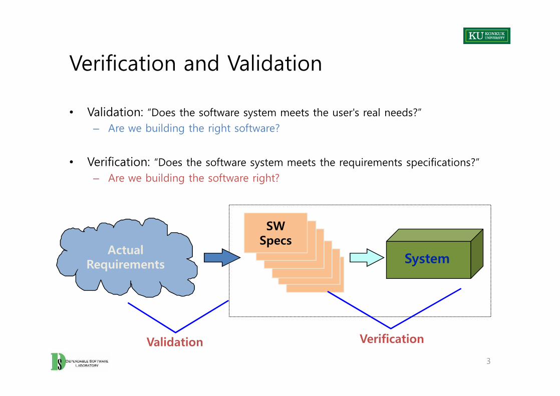
• Validation: “Does the software system meets the user's real needs?”– Are we building the right software?
• Verification: “Does the software system meets the requirements specifications?”– Are we building the software right?
ActualRequirements
SWSpecs
System
Validation Verification
3
V&V Depends on the Specification
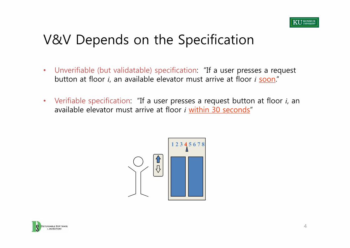
• Unverifiable (but validatable) specification: “If a user presses a request button at floor i, an available elevator must arrive at floor i soon.“
• Verifiable specification: “If a user presses a request button at floor i, an available elevator must arrive at floor i within 30 seconds“
• Unverifiable (but validatable) specification: “If a user presses a request button at floor i, an available elevator must arrive at floor i soon.“
• Verifiable specification: “If a user presses a request button at floor i, an available elevator must arrive at floor i within 30 seconds“
4
1 2 3 4 5 6 7 8
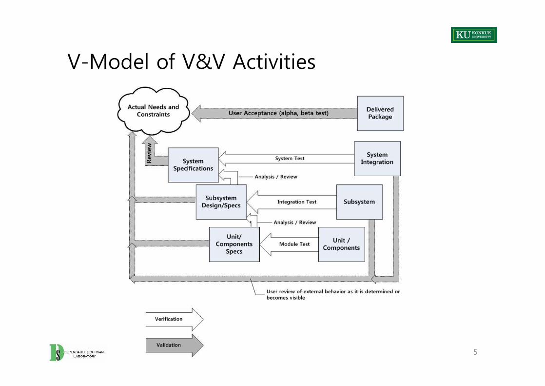
V-Model of V&V Activities
5
Undeciability of Correctness Properties
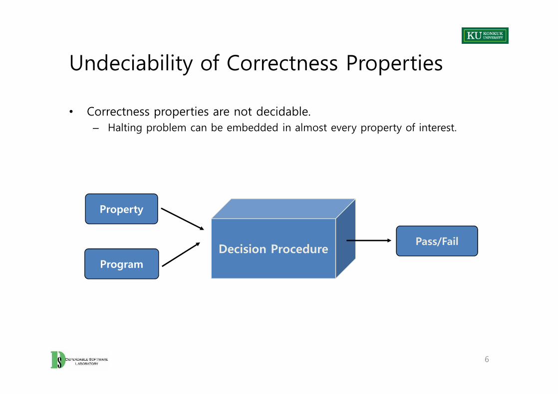
• Correctness properties are not decidable.– Halting problem can be embedded in almost every property of interest.
6
Decision Procedure
Property
Program
Pass/Fail
Verification Trade-off Dimensions
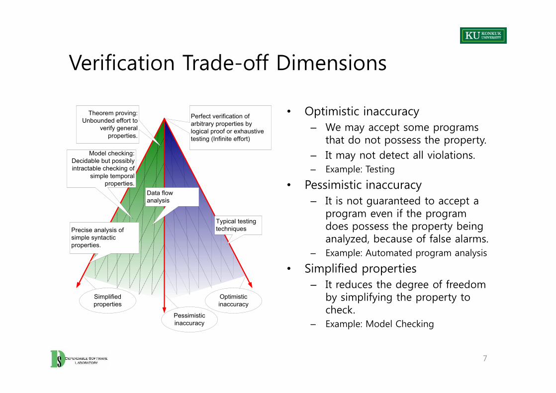
• Optimistic inaccuracy– We may accept some programs
that do not possess the property.– It may not detect all violations. – Example: Testing
• Pessimistic inaccuracy– It is not guaranteed to accept a
program even if the program does possess the property being analyzed, because of false alarms.
– Example: Automated program analysis
• Simplified properties– It reduces the degree of freedom
by simplifying the property to check.
– Example: Model Checking
Perfect verification ofarbitrary properties bylogical proof or exhaustivetesting (Infinite effort)
Model checking:Decidable but possiblyintractable checking of
simple temporalproperties.
Theorem proving:Unbounded effort to
verify generalproperties.
Data flow
• Optimistic inaccuracy– We may accept some programs
that do not possess the property.– It may not detect all violations. – Example: Testing
• Pessimistic inaccuracy– It is not guaranteed to accept a
program even if the program does possess the property being analyzed, because of false alarms.
– Example: Automated program analysis
• Simplified properties– It reduces the degree of freedom
by simplifying the property to check.
– Example: Model Checking
7
Precise analysis ofsimple syntacticproperties.
Typical testingtechniques
analysis
Optimisticinaccuracy
Pessimisticinaccuracy
Simplifiedproperties
Software Quality and Process
• Qualities cannot be added after development– Quality results from a set of inter-dependent activities.– Analysis and testing are crucial but far from sufficient.
• Testing is not a phase, but a lifestyle– Testing and analysis activities occur from early in requirements engineering
through delivery and subsequent evolution. – Quality depends on every part of the software process.
• An essential feature of software processes is that software test and analysis is thoroughly integrated and not an afterthought
8
Quality Process
• Quality process– A set of activities and responsibilities
• Focused on ensuring adequate dependability • Concerned with project schedule or with product usability
• Quality process provides a framework for – Selecting and arranging A&T activities – Considering interactions and trade-offs with other important goals
9
Planning and Monitoring
• Quality process – A&T planning– Balances several activities across the whole development process– Selects and arranges them to be as cost-effective as possible– Improves early visibility
• A&T planning is integral to the quality process.– Quality goals can be achieved only through careful planning.
10
Quality Goals
• Goal must be further refined into a clear and reasonable set of objectives.
• Product quality: goals of software quality engineering• Process quality: means to achieve the goals
• Product qualities– Internal qualities: invisible to clients
• maintainability, flexibility, reparability, changeability– External qualities: directly visible to clients
• Usefulness:– usability, performance, security, portability, interoperability
• Dependability:– correctness, reliability, safety, robustness
11
Dependability Properties
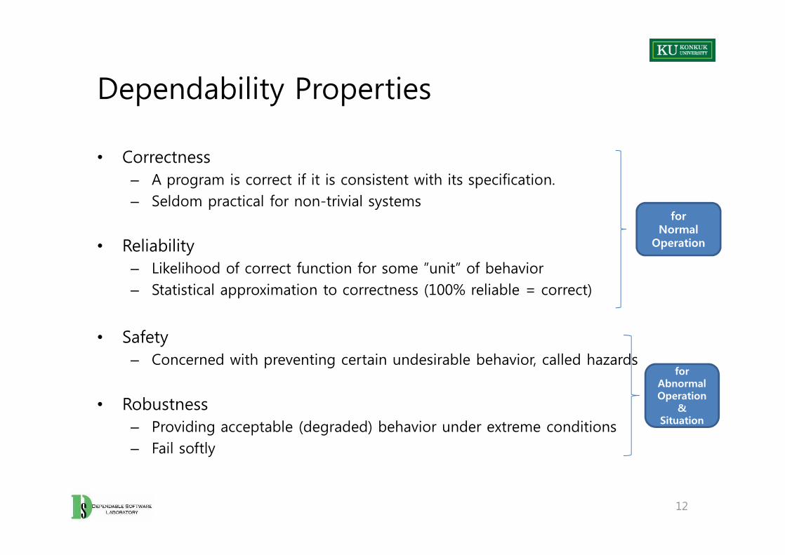
• Correctness– A program is correct if it is consistent with its specification.– Seldom practical for non-trivial systems
• Reliability– Likelihood of correct function for some ”unit” of behavior– Statistical approximation to correctness (100% reliable = correct)
• Safety– Concerned with preventing certain undesirable behavior, called hazards
• Robustness– Providing acceptable (degraded) behavior under extreme conditions– Fail softly
for Normal
Operation
• Correctness– A program is correct if it is consistent with its specification.– Seldom practical for non-trivial systems
• Reliability– Likelihood of correct function for some ”unit” of behavior– Statistical approximation to correctness (100% reliable = correct)
• Safety– Concerned with preventing certain undesirable behavior, called hazards
• Robustness– Providing acceptable (degraded) behavior under extreme conditions– Fail softly
12
for Abnormal Operation
&Situation
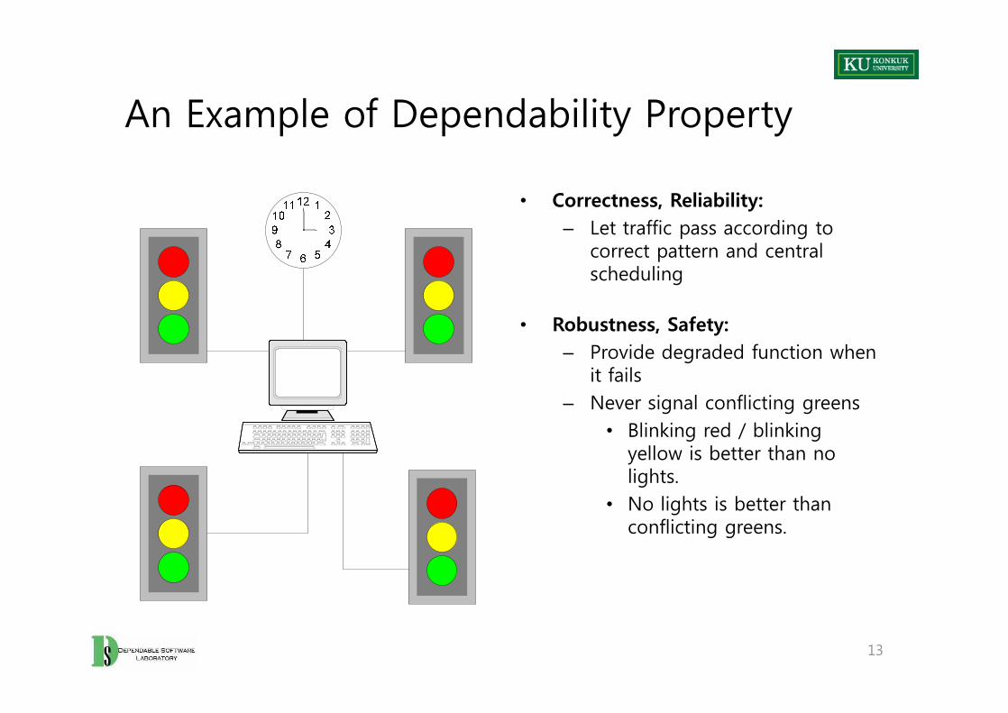
An Example of Dependability Property
• Correctness, Reliability: – Let traffic pass according to
correct pattern and central scheduling
• Robustness, Safety: – Provide degraded function when
it fails– Never signal conflicting greens
• Blinking red / blinking yellow is better than no lights.
• No lights is better than conflicting greens.
13

14
Part II. Basic Techniques
Model
• A model is– A representation that is simpler than the artifact it represents,– But preserves some important attributes of the actual artifact
• Our concern is with models of program execution.
16
Intraprocedural Control Flow Graph
• Called “Control Flow Graph” or “CGF”– A directed graph (N, E)
• Nodes – Regions of source code (basic blocks)– Basic block = maximal program region with a single entry and single exit
point– Statements are often grouped in single regions to get a compact model.– Sometime single statements are broken into more than one node to model
control flow within the statement.
• Directed edges – Possibility that program execution proceeds from the end of one region
directly to the beginning of another
17
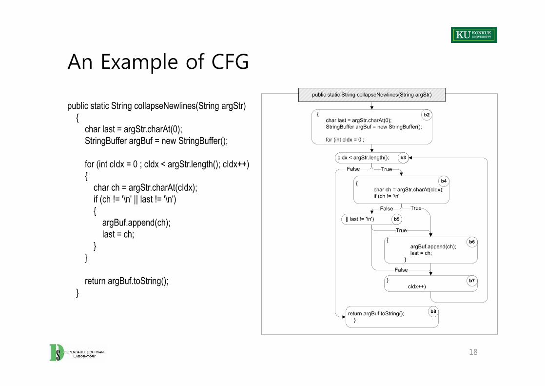
An Example of CFG
public static String collapseNewlines(String argStr){
char last = argStr.charAt(0);StringBuffer argBuf = new StringBuffer();
for (int cIdx = 0 ; cIdx < argStr.length(); cIdx++){
char ch = argStr.charAt(cIdx);if (ch != '\n' || last != '\n'){
argBuf.append(ch);last = ch;
}}
return argBuf.toString();}
{char last = argStr.charAt(0);StringBuffer argBuf = new StringBuffer();
for (int cIdx = 0 ;
{char ch = argStr.charAt(cIdx);
cIdx < argStr.length();
True
public static String collapseNewlines(String argStr)
False
b2
b4
b3
public static String collapseNewlines(String argStr){
char last = argStr.charAt(0);StringBuffer argBuf = new StringBuffer();
for (int cIdx = 0 ; cIdx < argStr.length(); cIdx++){
char ch = argStr.charAt(cIdx);if (ch != '\n' || last != '\n'){
argBuf.append(ch);last = ch;
}}
return argBuf.toString();}
18
if (ch != '\n'
True
{argBuf.append(ch);last = ch;
}
True
}cIdx++)
return argBuf.toString();}
False
False
|| last != '\n') b5
b6
b7
b8
Call Graphs
• “Interprocedural Control Flow Graph”– A directed graph (N, E)
• Nodes– Represent procedures, methods, functions, etc.
• Edges– Represent ‘call’ relation
• Call graph presents many more design issues and trade-off than CFG.– Overestimation of call relation– Context sensitive/insensitive
• “Interprocedural Control Flow Graph”– A directed graph (N, E)
• Nodes– Represent procedures, methods, functions, etc.
• Edges– Represent ‘call’ relation
• Call graph presents many more design issues and trade-off than CFG.– Overestimation of call relation– Context sensitive/insensitive
19
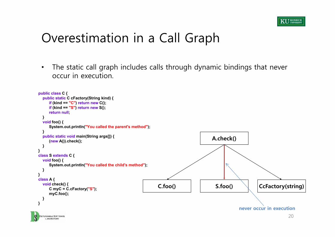
Overestimation in a Call Graph
• The static call graph includes calls through dynamic bindings that never occur in execution.
public class C {public static C cFactory(String kind) {
if (kind == "C") return new C(); if (kind == "S") return new S(); return null;
}void foo() {
System.out.println("You called the parent's method"); }public static void main(String args[]) {
(new A()).check(); }
}class S extends C {
void foo() {System.out.println("You called the child's method");
}}class A {
void check() { C myC = C.cFactory("S"); myC.foo();
}}
• The static call graph includes calls through dynamic bindings that never occur in execution.
20
public class C {public static C cFactory(String kind) {
if (kind == "C") return new C(); if (kind == "S") return new S(); return null;
}void foo() {
System.out.println("You called the parent's method"); }public static void main(String args[]) {
(new A()).check(); }
}class S extends C {
void foo() {System.out.println("You called the child's method");
}}class A {
void check() { C myC = C.cFactory("S"); myC.foo();
}}
A.check()
C.foo() S.foo() CcFactory(string)
never occur in execution
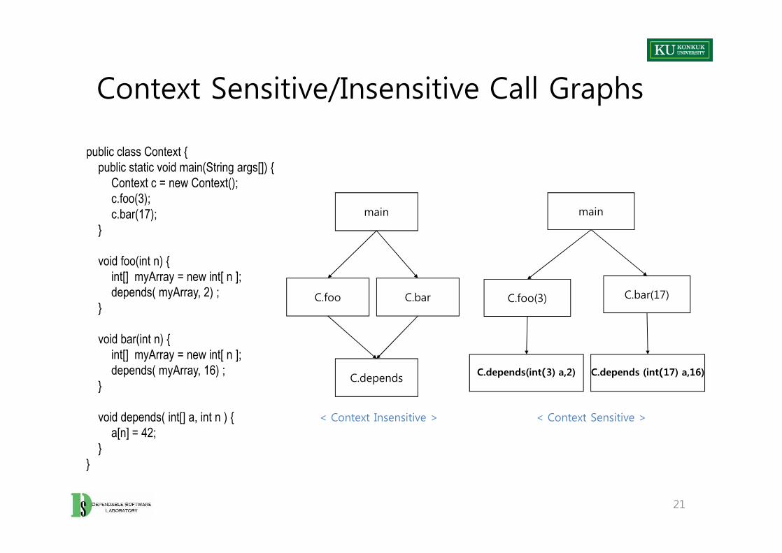
Context Sensitive/Insensitive Call Graphs
public class Context {public static void main(String args[]) {
Context c = new Context(); c.foo(3); c.bar(17);
}
void foo(int n) {int[] myArray = new int[ n ]; depends( myArray, 2) ;
}
void bar(int n) {int[] myArray = new int[ n ]; depends( myArray, 16) ;
}
void depends( int[] a, int n ) {a[n] = 42;
}}
main main
21
public class Context {public static void main(String args[]) {
Context c = new Context(); c.foo(3); c.bar(17);
}
void foo(int n) {int[] myArray = new int[ n ]; depends( myArray, 2) ;
}
void bar(int n) {int[] myArray = new int[ n ]; depends( myArray, 16) ;
}
void depends( int[] a, int n ) {a[n] = 42;
}}
C.foo C.bar
C.depends
C.foo(3) C.bar(17)
C.depends(int(3) a,2) C.depends (int(17) a,16)
< Context Insensitive > < Context Sensitive >
Finite State Machines
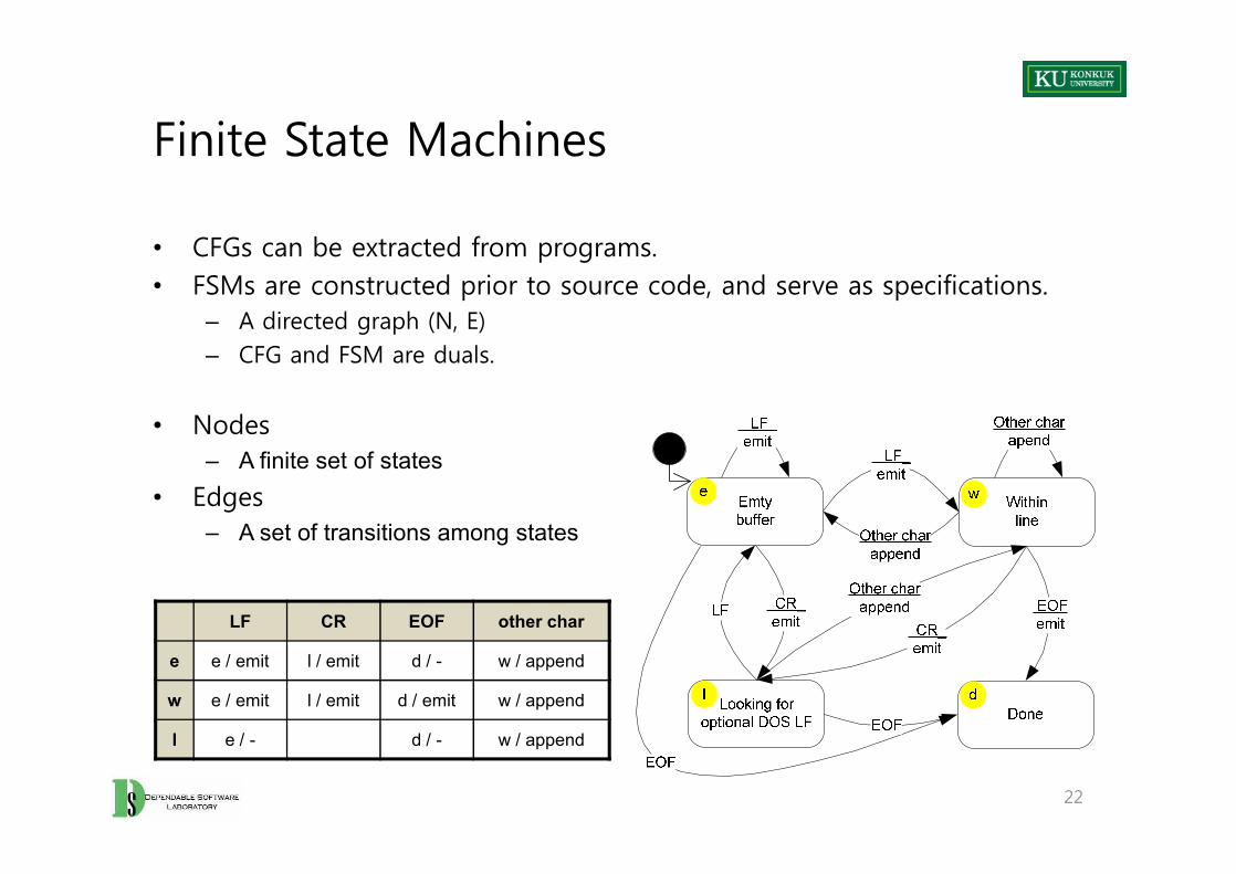
• CFGs can be extracted from programs.• FSMs are constructed prior to source code, and serve as specifications.
– A directed graph (N, E)– CFG and FSM are duals.
• Nodes– A finite set of states
• Edges– A set of transitions among states
• CFGs can be extracted from programs.• FSMs are constructed prior to source code, and serve as specifications.
– A directed graph (N, E)– CFG and FSM are duals.
• Nodes– A finite set of states
• Edges– A set of transitions among states
22
LF CR EOF other char
e e / emit l / emit d / - w / append
w e / emit l / emit d / emit w / append
l e / - d / - w / append
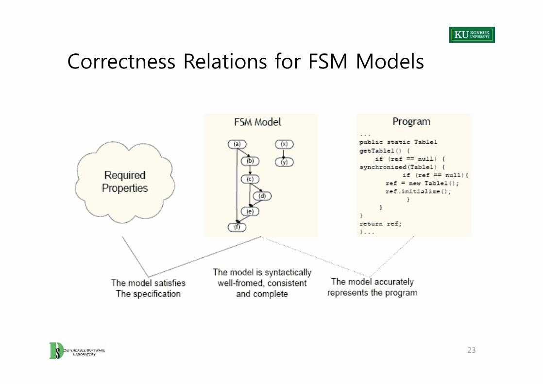
Correctness Relations for FSM Models
23
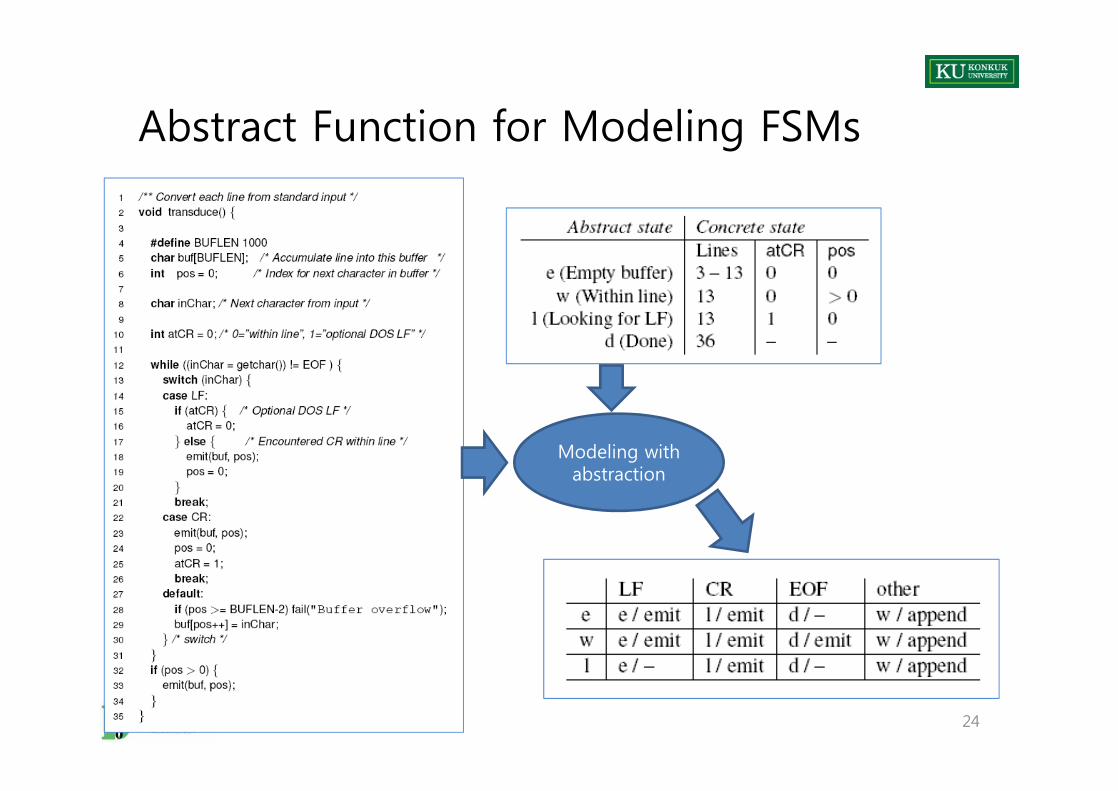
Abstract Function for Modeling FSMs
24
Modeling with abstraction
Why Data Flow Models Need?
• Models from Chapter 5 emphasized control flow only.– Control flow graph, call graph, finite state machine
• We also need to reason about data dependence.– To reason about transmission of information through program variables– “Where does this value of x come from?”– “What would be affected by changing this? “– ...
• Many program analyses and test design techniques use data flow information and dependences
– Often in combination with control flow
25
Definition-Use Pairs
• A def-use (du) pair associates a point in a program where a value is produced with a point where it is used
• Definition: where a variable gets a value– Variable declaration– Variable initialization– Assignment– Values received by a parameter
• Use: extraction of a value from a variable– Expressions– Conditional statements– Parameter passing– Returns
26
Def-Use Pairs
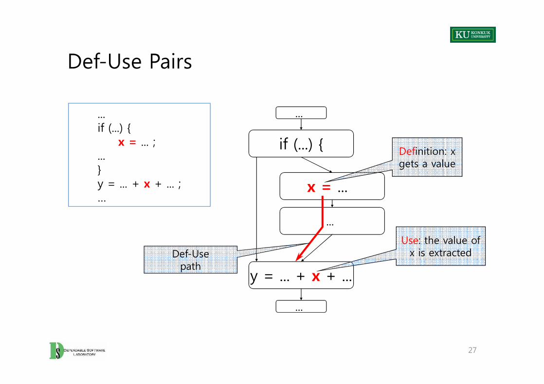
...if (...) {
x = ... ; ... }y = ... + x + ... ;…
x = ...
if (...) {
...
Definition: x gets a value
27
...if (...) {
x = ... ; ... }y = ... + x + ... ;…
x = ...
...
y = ... + x + ...
...
Use: the value of x is extractedDef-Use
path
Definition-Clear & Killing
• A definition-clear path is a path along the CFG from a definition to a use of the same variable without another definition of the variable between.
• If, instead, another definition is present on the path, then the latter definition kills the former
• A def-use pair is formed if and only if there is a definition-clear path between the definition and the use
28
Definition-Clear & Killing
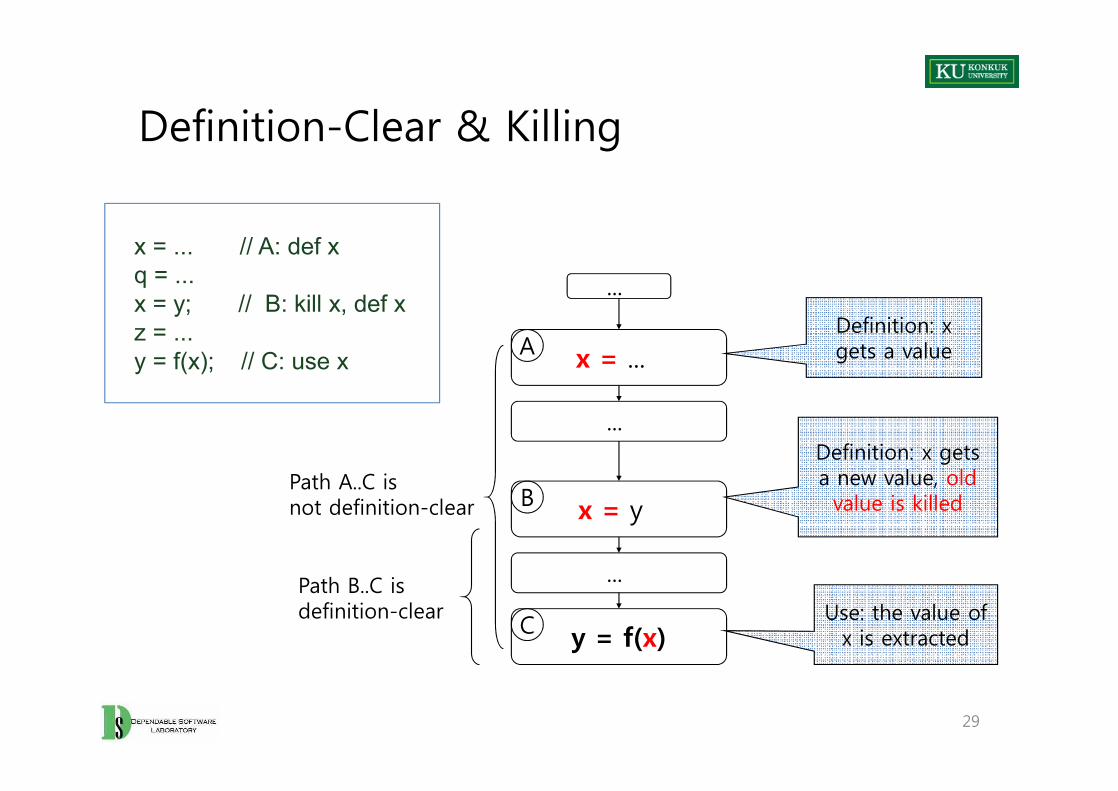
x = ... // A: def xq = ... x = y; // B: kill x, def xz = ... y = f(x); // C: use x x = ...
...
Definition: x gets a valueA
29
...
Use: the value of x is extracted
x = y
Definition: x gets a new value, old value is killed
...
y = f(x)
B
C
Path B..C is definition-clear
Path A..C is not definition-clear
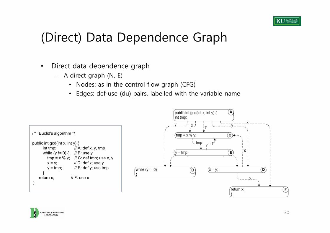
(Direct) Data Dependence Graph
• Direct data dependence graph– A direct graph (N, E)
• Nodes: as in the control flow graph (CFG)• Edges: def-use (du) pairs, labelled with the variable name
30
x
/** Euclid's algorithm */
public int gcd(int x, int y) {int tmp; // A: def x, y, tmp while (y != 0) { // B: use y
tmp = x % y; // C: def tmp; use x, yx = y; // D: def x; use yy = tmp; // E: def y; use tmp
}return x; // F: use x
}
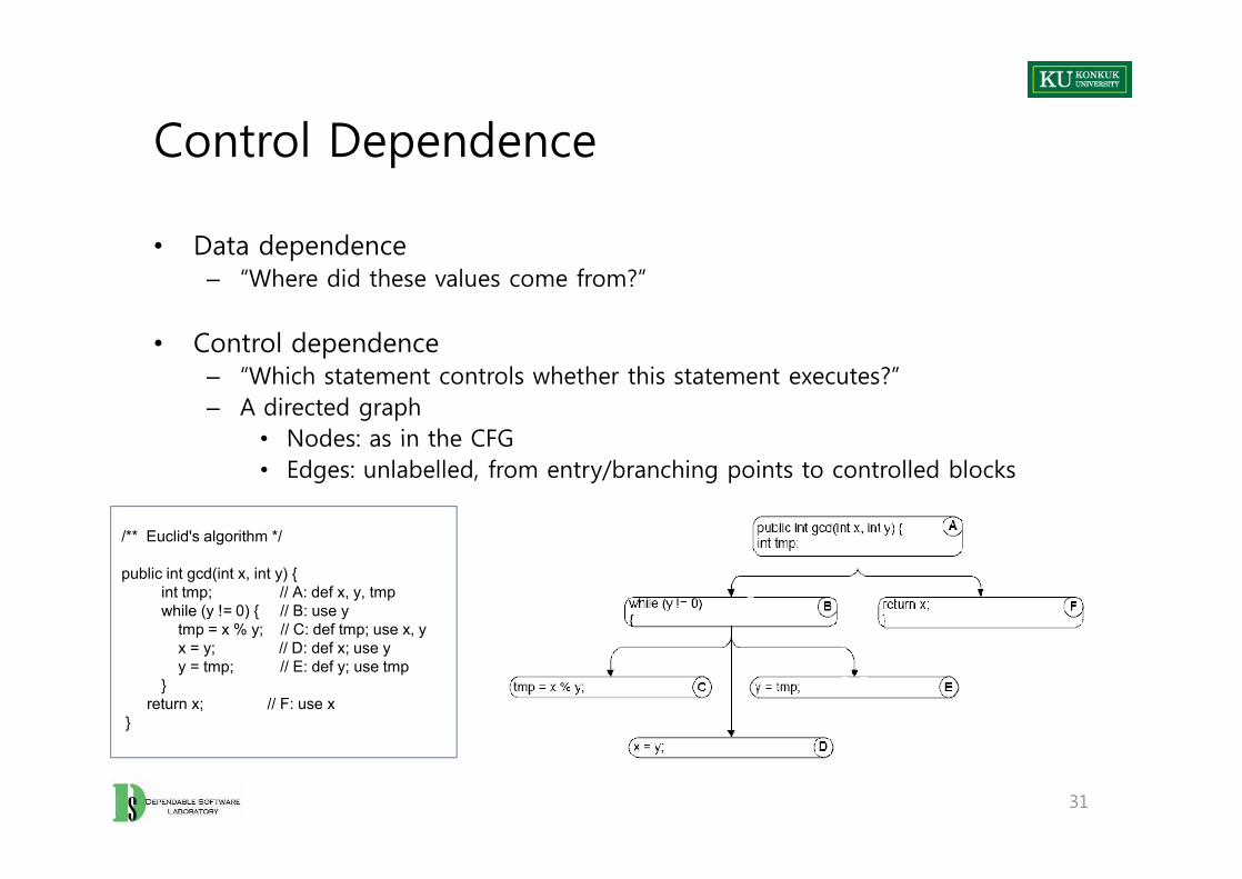
Control Dependence
• Data dependence– “Where did these values come from?”
• Control dependence – “Which statement controls whether this statement executes?”– A directed graph
• Nodes: as in the CFG• Edges: unlabelled, from entry/branching points to controlled blocks
• Data dependence– “Where did these values come from?”
• Control dependence – “Which statement controls whether this statement executes?”– A directed graph
• Nodes: as in the CFG• Edges: unlabelled, from entry/branching points to controlled blocks
31
/** Euclid's algorithm */
public int gcd(int x, int y) {int tmp; // A: def x, y, tmp while (y != 0) { // B: use y
tmp = x % y; // C: def tmp; use x, yx = y; // D: def x; use yy = tmp; // E: def y; use tmp
}return x; // F: use x
}
Dominator
• Pre-dominators in a rooted, directed graph can be used to make this intuitive notion of “controlling decision” precise.
• Node M dominates node N, if every path from the root to N passes through M.
– A node will typically have many dominators, but except for the root, there is a unique immediate dominator of node N which is closest to N on any path from the root, and which is in turn dominated by all the other dominators of N.
– Because each node (except the root) has a unique immediate dominator, the immediate dominator relation forms a tree.
• Post-dominators are calculated in the reverse of the control flow graph, using a special “exit” node as the root.
32
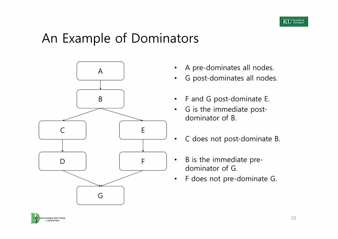
An Example of Dominators
• A pre-dominates all nodes.• G post-dominates all nodes.
• F and G post-dominate E.• G is the immediate post-
dominator of B.
• C does not post-dominate B.
• B is the immediate pre-dominator of G.
• F does not pre-dominate G.
A
B
• A pre-dominates all nodes.• G post-dominates all nodes.
• F and G post-dominate E.• G is the immediate post-
dominator of B.
• C does not post-dominate B.
• B is the immediate pre-dominator of G.
• F does not pre-dominate G.
33
C
D
E
F
G
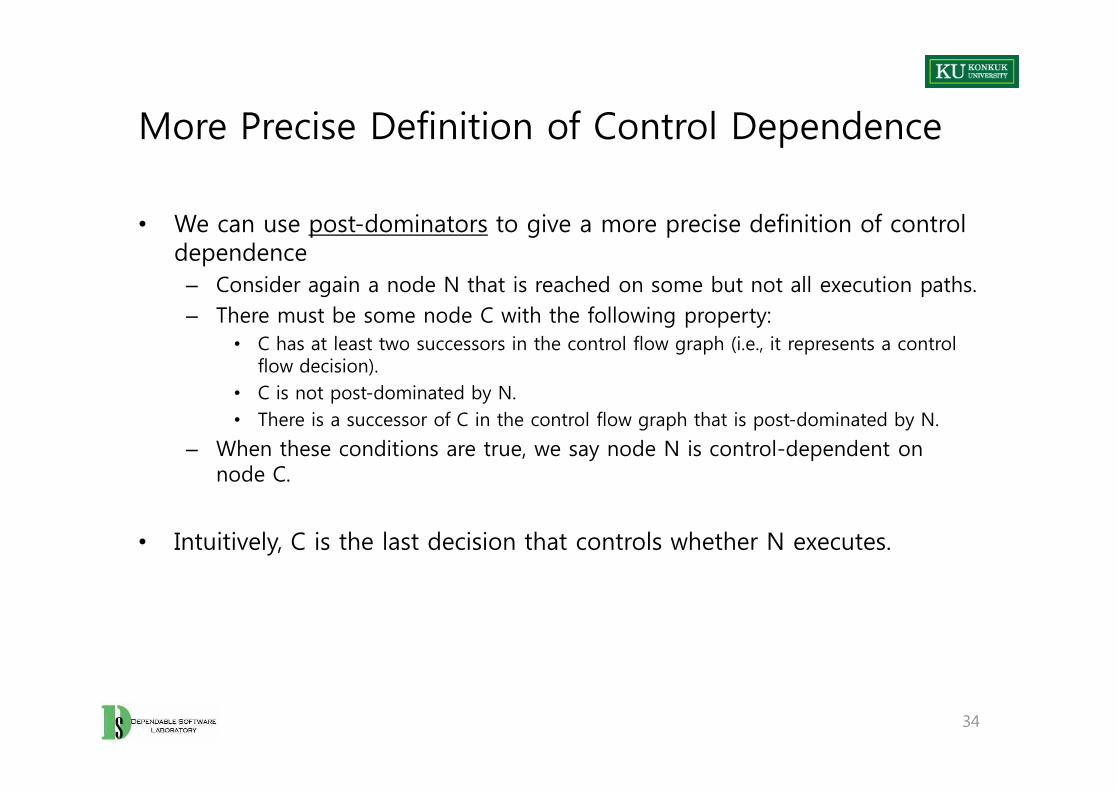
More Precise Definition of Control Dependence
• We can use post-dominators to give a more precise definition of control dependence
– Consider again a node N that is reached on some but not all execution paths.– There must be some node C with the following property:
• C has at least two successors in the control flow graph (i.e., it represents a control flow decision).
• C is not post-dominated by N.• There is a successor of C in the control flow graph that is post-dominated by N.
– When these conditions are true, we say node N is control-dependent on node C.
• Intuitively, C is the last decision that controls whether N executes.
34
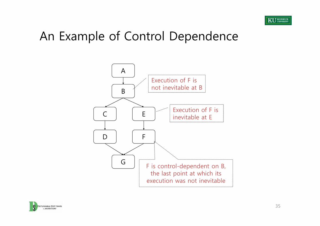
An Example of Control Dependence
A
B
C E
Execution of F is not inevitable at B
Execution of F is inevitable at E
35
C
D
E
F
GF is control-dependent on B,
the last point at which itsexecution was not inevitable
Execution of F is inevitable at E
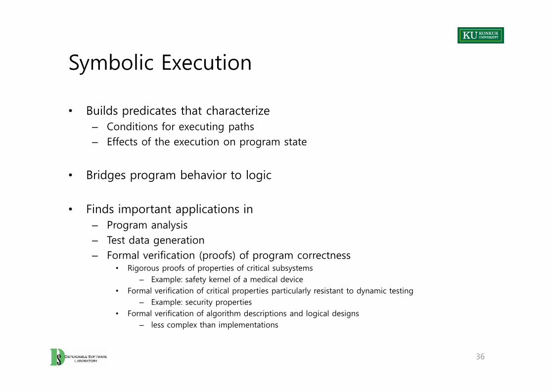
Symbolic Execution
• Builds predicates that characterize – Conditions for executing paths – Effects of the execution on program state
• Bridges program behavior to logic
• Finds important applications in – Program analysis– Test data generation– Formal verification (proofs) of program correctness
• Rigorous proofs of properties of critical subsystems– Example: safety kernel of a medical device
• Formal verification of critical properties particularly resistant to dynamic testing – Example: security properties
• Formal verification of algorithm descriptions and logical designs– less complex than implementations
36
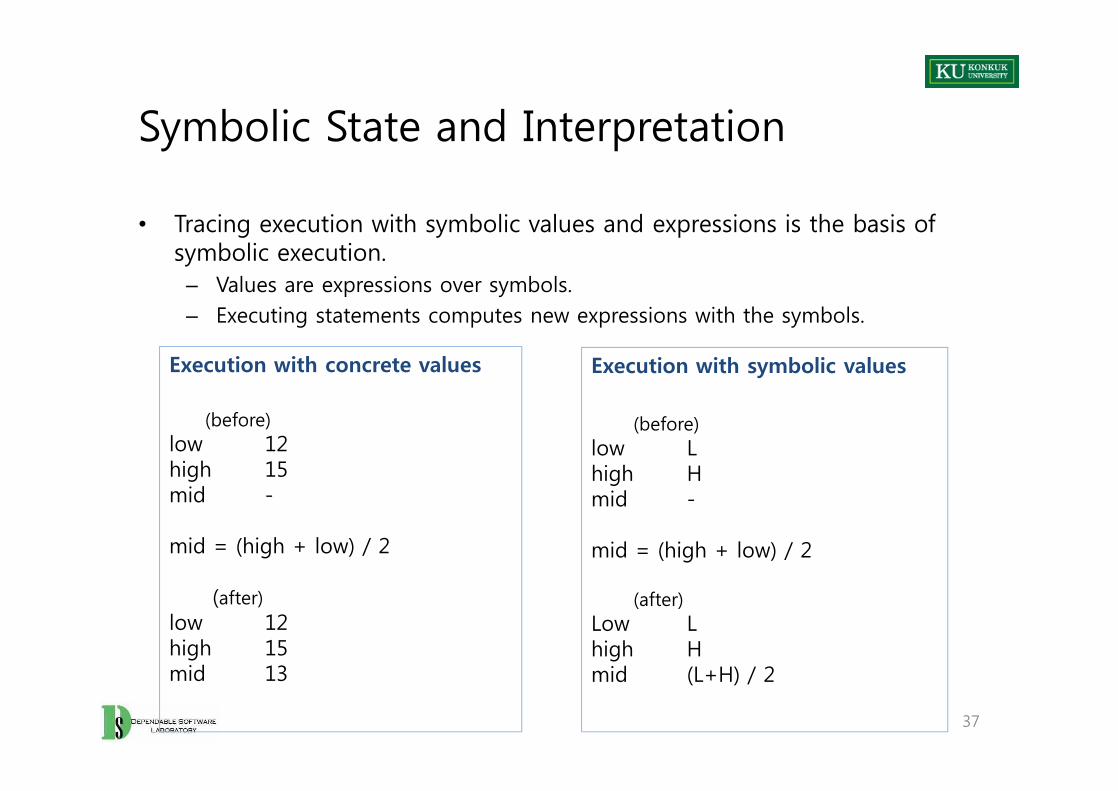
Symbolic State and Interpretation
• Tracing execution with symbolic values and expressions is the basis of symbolic execution.
– Values are expressions over symbols.– Executing statements computes new expressions with the symbols.
Execution with concrete values
(before)low 12high 15mid -
mid = (high + low) / 2
(after)low 12high 15mid 13
Execution with symbolic values
(before)low Lhigh Hmid -
mid = (high + low) / 2
(after)Low Lhigh Hmid (L+H) / 2
37
Execution with concrete values
(before)low 12high 15mid -
mid = (high + low) / 2
(after)low 12high 15mid 13
Execution with symbolic values
(before)low Lhigh Hmid -
mid = (high + low) / 2
(after)Low Lhigh Hmid (L+H) / 2
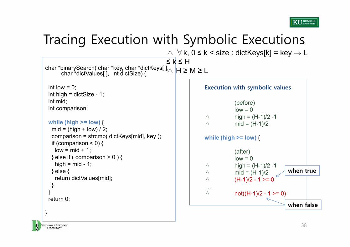
Tracing Execution with Symbolic Executions
char *binarySearch( char *key, char *dictKeys[ ], char *dictValues[ ], int dictSize) {
int low = 0; int high = dictSize - 1; int mid; int comparison;
while (high >= low) {mid = (high + low) / 2; comparison = strcmp( dictKeys[mid], key );if (comparison < 0) {low = mid + 1;
} else if ( comparison > 0 ) {high = mid - 1;
} else {return dictValues[mid];
}}return 0;
}
Execution with symbolic values
(before)low = 0
∧ high = (H-1)/2 -1∧ mid = (H-1)/2
while (high >= low) {
(after)low = 0
∧ high = (H-1)/2 -1∧ mid = (H-1)/2∧ (H-1)/2 - 1 >= 0... ∧ not((H-1)/2 - 1 >= 0)
∧∀k, 0 ≤ k < size : dictKeys[k] = key → L ≤ k ≤ H∧ H ≥ M ≥ L
38
char *binarySearch( char *key, char *dictKeys[ ], char *dictValues[ ], int dictSize) {
int low = 0; int high = dictSize - 1; int mid; int comparison;
while (high >= low) {mid = (high + low) / 2; comparison = strcmp( dictKeys[mid], key );if (comparison < 0) {low = mid + 1;
} else if ( comparison > 0 ) {high = mid - 1;
} else {return dictValues[mid];
}}return 0;
}
Execution with symbolic values
(before)low = 0
∧ high = (H-1)/2 -1∧ mid = (H-1)/2
while (high >= low) {
(after)low = 0
∧ high = (H-1)/2 -1∧ mid = (H-1)/2∧ (H-1)/2 - 1 >= 0... ∧ not((H-1)/2 - 1 >= 0)
when true
when false
Summary Information
• Symbolic representation of paths may become extremely complex.
• We can simplify the representation by replacing a complex condition Pwith a weaker condition W such that
P => W– W describes the path with less precision– W is a summary of P
• Symbolic representation of paths may become extremely complex.
• We can simplify the representation by replacing a complex condition Pwith a weaker condition W such that
P => W– W describes the path with less precision– W is a summary of P
39
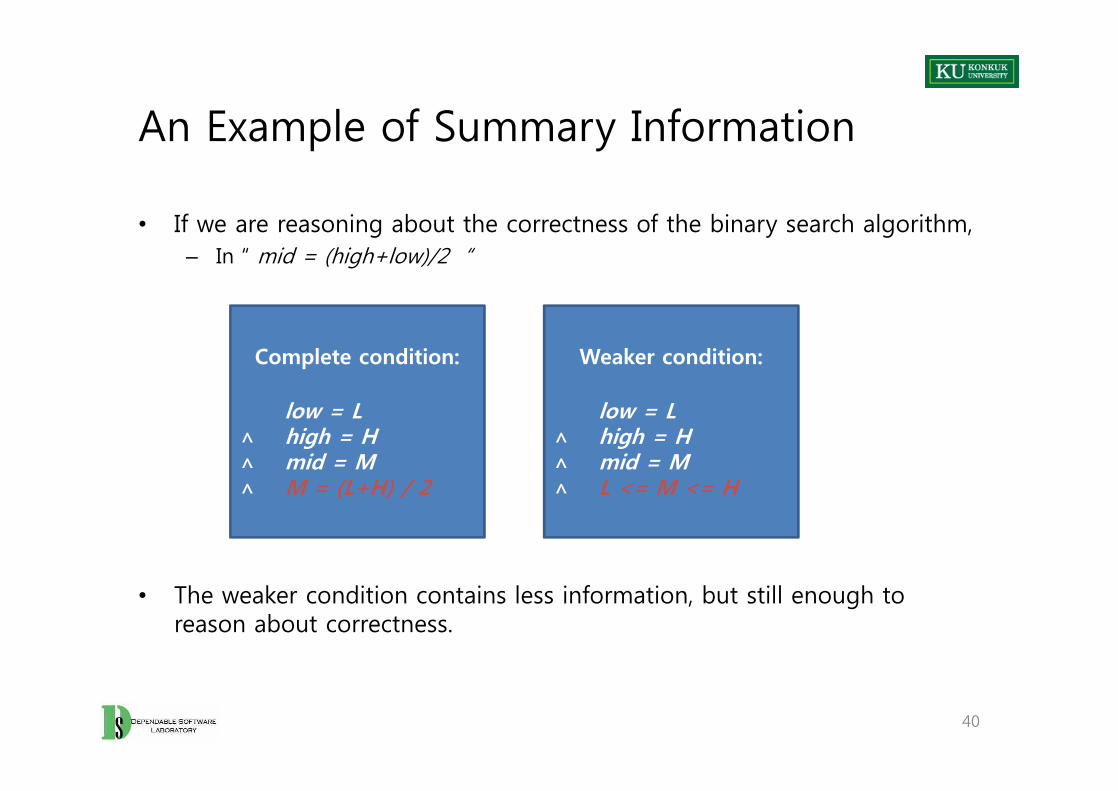
An Example of Summary Information
• If we are reasoning about the correctness of the binary search algorithm, – In “ mid = (high+low)/2 “
• The weaker condition contains less information, but still enough to reason about correctness.
Weaker condition:
low = L∧ high = H∧ mid = M∧ L <= M <= H
Complete condition:
low = L∧ high = H∧ mid = M∧ M = (L+H) / 2
• If we are reasoning about the correctness of the binary search algorithm, – In “ mid = (high+low)/2 “
• The weaker condition contains less information, but still enough to reason about correctness.
40
Weaker condition:
low = L∧ high = H∧ mid = M∧ L <= M <= H
Complete condition:
low = L∧ high = H∧ mid = M∧ M = (L+H) / 2
Compositional Reasoning
• Follow the hierarchical structure of a program– at a small scale (within a single procedure) – at larger scales (across multiple procedures)
• Hoare triple: [pre] block [post]
• If the program is in a state satisfying the precondition pre at entry to the block, then after execution of the block, it will be in a state satisfying the postcondition post
41
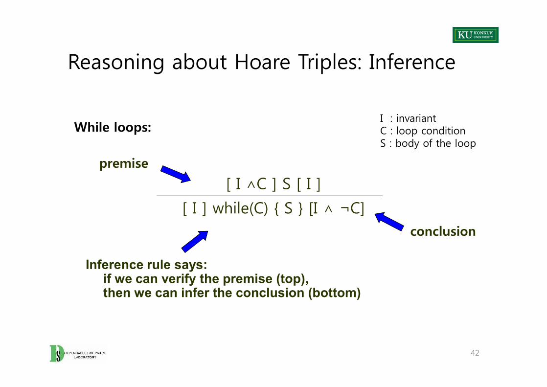
Reasoning about Hoare Triples: Inference
[ I ∧C ] S [ I ]
[ I ] while(C) { S } [I ∧ ¬C]
premise
While loops:I : invariantC : loop conditionS : body of the loop
42
[ I ∧C ] S [ I ]
[ I ] while(C) { S } [I ∧ ¬C]
Inference rule says:if we can verify the premise (top), then we can infer the conclusion (bottom)
conclusion
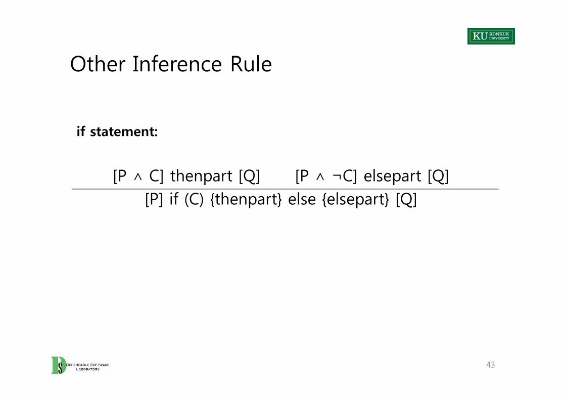
Other Inference Rule
if statement:
[P ∧ C] thenpart [Q] [P ∧ ¬C] elsepart [Q][P] if (C) {thenpart} else {elsepart} [Q]
43
[P ∧ C] thenpart [Q] [P ∧ ¬C] elsepart [Q][P] if (C) {thenpart} else {elsepart} [Q]
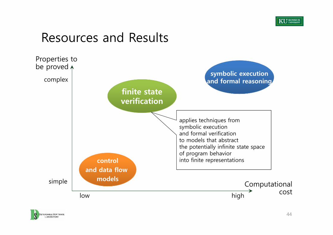
Resources and Results
Properties to be proved
complexsymbolic execution
and formal reasoningsymbolic execution
and formal reasoning
finite stateverificationfinite stateverification
applies techniques fromsymbolic executionand formal verificationto models that abstractthe potentially infinite state spaceof program behaviorinto finite representations
44
Computational costhighlow
simple
controland data flow
models
controland data flow
models
applies techniques fromsymbolic executionand formal verificationto models that abstractthe potentially infinite state spaceof program behaviorinto finite representations
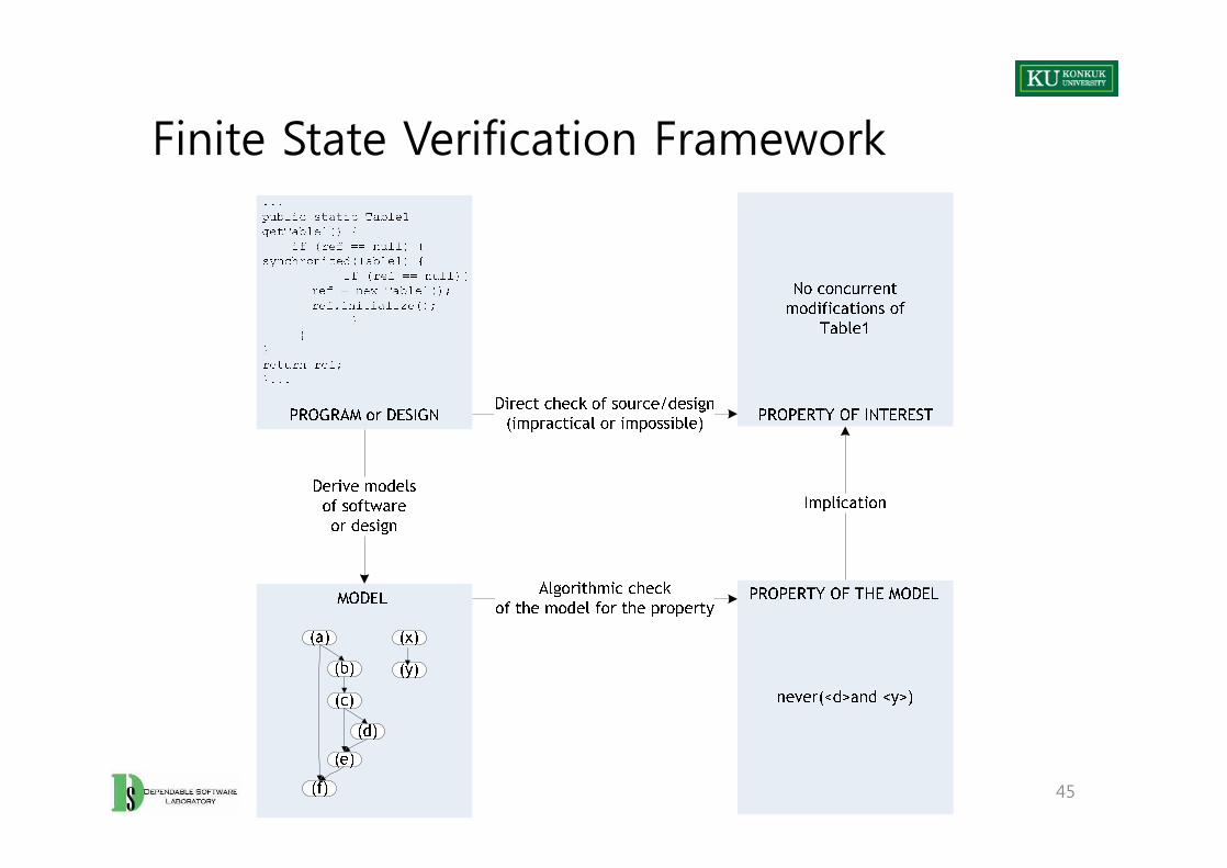
Finite State Verification Framework
45
The State Space Explosion Problem
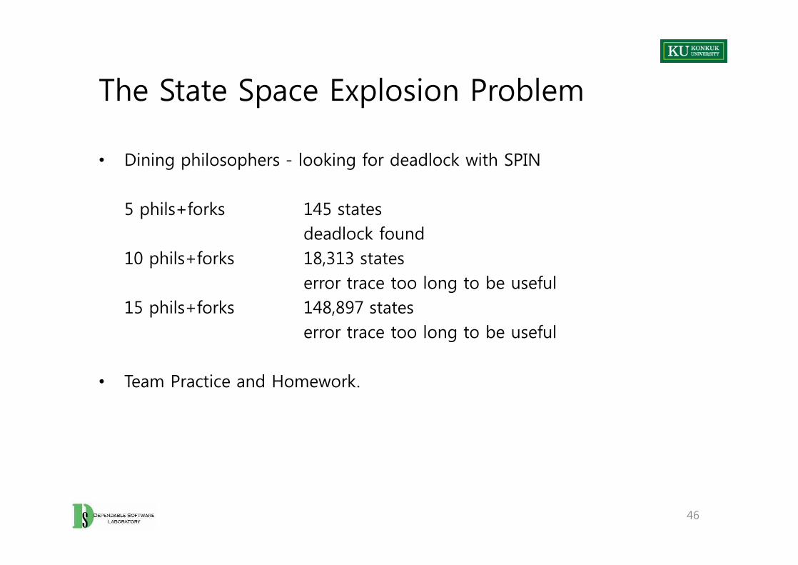
• Dining philosophers - looking for deadlock with SPIN
5 phils+forks 145 statesdeadlock found
10 phils+forks 18,313 stateserror trace too long to be useful
15 phils+forks 148,897 stateserror trace too long to be useful
• Team Practice and Homework.
• Dining philosophers - looking for deadlock with SPIN
5 phils+forks 145 statesdeadlock found
10 phils+forks 18,313 stateserror trace too long to be useful
15 phils+forks 148,897 stateserror trace too long to be useful
• Team Practice and Homework.
46
The Model Correspondence Problem
• Verifying correspondence between model and program– Extract the model from the source code with verified procedures
• Blindly mirroring all details à state space explosion • Omitting crucial detail à “false alarm” reports
– Produce the source code automatically from the model• Most applicable within well-understood domains
– Conformance testing• Combination of FSV and testing is a good tradeoff
47
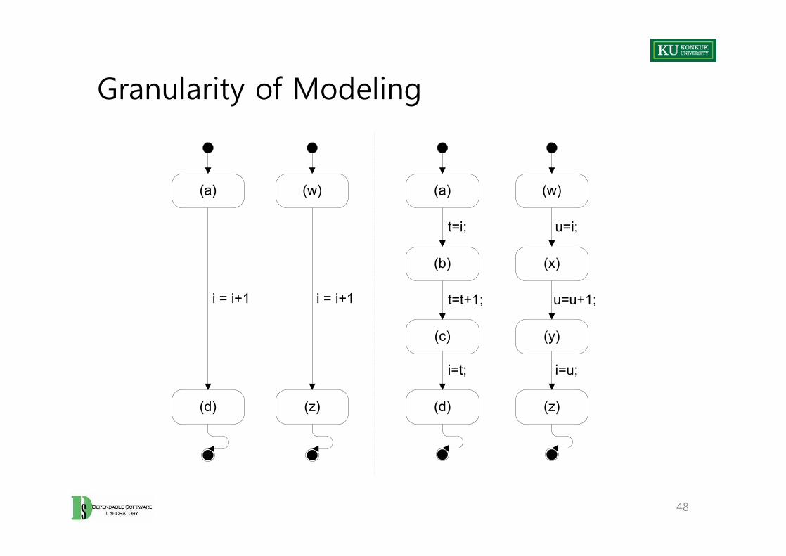
Granularity of Modeling
(a) (a)
(b)
t=i;
(w)
(x)
u=i;
(w)
48
(d)
i = i+1
E E
(c)
t=t+1;
(d)
i=t;
E
(y)
u=u+1;
(z)
i=u;
(z)
i = i+1
E
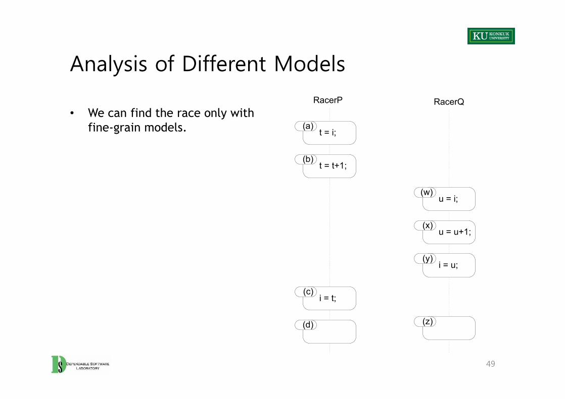
Analysis of Different Models
• We can find the race only with fine-grain models.
RacerP RacerQ
t = i;(a)
t = t+1;(b)
u = i;(w)
49
i = t;(c)
(d)
u = i;
u = u+1;(x)
i = u;(y)
(z)

Intentional Models
• Enumerating all reachable states is a limiting factor of finite state verification.
• We can reduce the space by using intentional (symbolic) representations.– describe sets of reachable states without enumerating each one individually
• Example (set of Integers)– Enumeration {2, 4, 6, 8, 10, 12, 14, 16, 18}– Intentional representation: {x∈N | x mod 2 =0 and 0<x<20} ← “characteristic function”
• Intentional models do not necessarily grow with the size of the set they represent
50
OBDD: A Useful Intentional Model
• OBDD (Ordered Binary Decision Diagram)– A compact representation of Boolean functions
• Characteristic function for transition relations– Transitions = pairs of states– Function from pairs of states to Booleans is true, if there is a transition
between the pair.– Built iteratively by breadth-first expansion of the state space:
• Create a representation of the whole set of states reachable in k+1 steps from the set of states reachable in k steps
• OBDD stabilizes when all the transitions that can occur in the next step are already represented in the OBDD.
51
From OBDD to Symbolic Checking
• Intentional representation itself is not enough.• We must have an algorithm for determining whether it satisfies the
property we are checking.
• Example: A set of communicating state machines using OBDD– To represent the transition relation of a set of communicating state machines– To model a class of temporal logic specification formulas
• Combine OBDD representations of model and specification to produce a representation of just the set of transitions leading to a violation of the specification
– If the set is empty, the property has been verified.
52
Representing Transition Relations as Boolean Functions
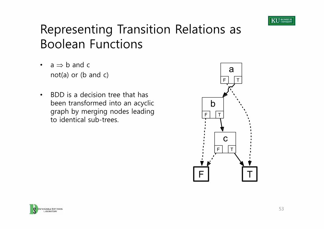
• a Þ b and cnot(a) or (b and c)
• BDD is a decision tree that has been transformed into an acyclic graph by merging nodes leading to identical sub-trees.
aF T
F T
bF T
cF T
• a Þ b and cnot(a) or (b and c)
• BDD is a decision tree that has been transformed into an acyclic graph by merging nodes leading to identical sub-trees.
53
aF T
F T
bF T
cF T
Representing Transition Relations as Boolean Functions : Steps
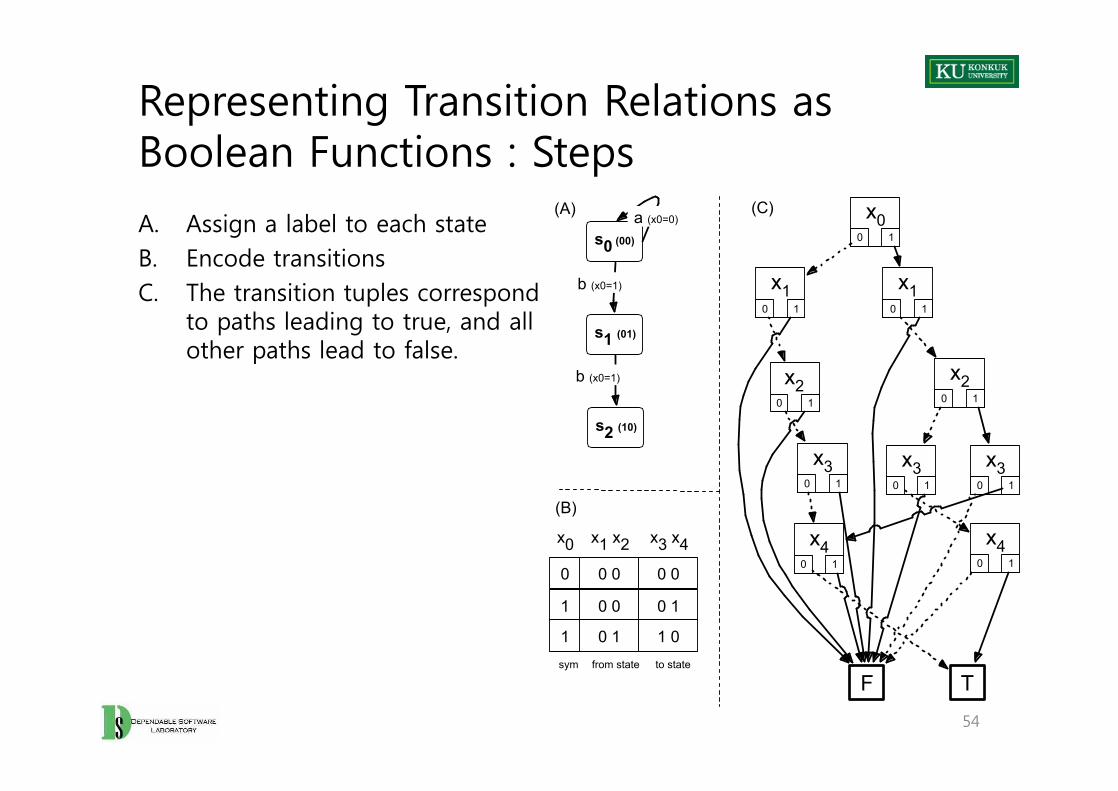
A. Assign a label to each stateB. Encode transitions C. The transition tuples correspond
to paths leading to true, and all other paths lead to false.
s0 (00)
s1 (01)
b (x0=1)
a (x0=0)
0 0 0 0 0
0 0 0 1 1
x1 x2 x3 x4 x0
x00 1
x10 1
F T
x10 1
x20 1
x30 1
x40 1
x20 1
x30 1
x40 1
sym from state to state
(A)
(B)
(C)
s2 (10)
b (x0=1)
0 1 1 0 1
x30 1
A. Assign a label to each stateB. Encode transitions C. The transition tuples correspond
to paths leading to true, and all other paths lead to false.
54
s0 (00)
s1 (01)
b (x0=1)
a (x0=0)
0 0 0 0 0
0 0 0 1 1
x1 x2 x3 x4 x0
x00 1
x10 1
F T
x10 1
x20 1
x30 1
x40 1
x20 1
x30 1
x40 1
sym from state to state
(A)
(B)
(C)
s2 (10)
b (x0=1)
0 1 1 0 1
x30 1
Intentional vs. Explicit Representations
• Worst case:– Given a large set S of states,– a representation capable of distinguishing each subset of S cannot be more
compact on average than the representation that simply lists elements of the chosen subset.
• Intentional representations work well when they exploit structure and regularity of the state space.
55
Model Refinement
• Construction of finite state models – Should balance precision and efficiency
• Often the first model is unsatisfactory – Report potential failures that are obviously impossible– Exhaust resources before producing any result
• Minor differences in the model can have large effects on tractability of the verification procedure.
• Finite state verification as iterative process is required.
56
Iteration Process
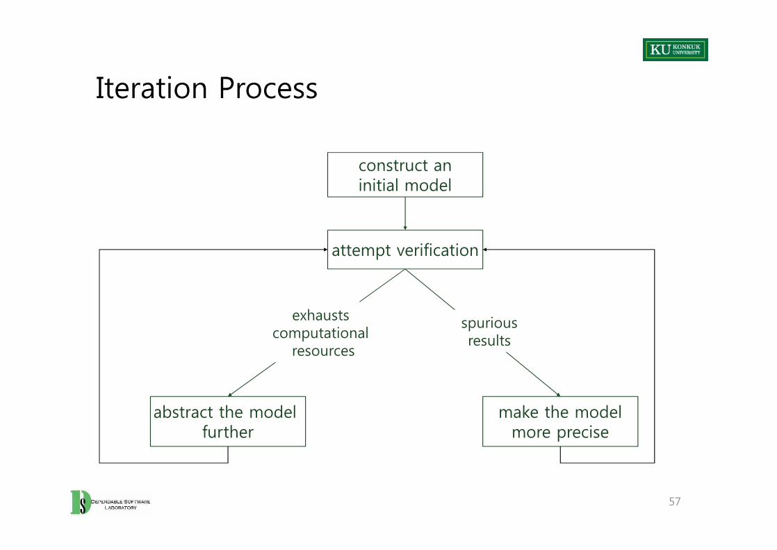
construct aninitial model
attempt verification
57
abstract the model further
exhausts computational
resources
make the modelmore precise
spuriousresults
Refinement 1: Adding Details to the Model
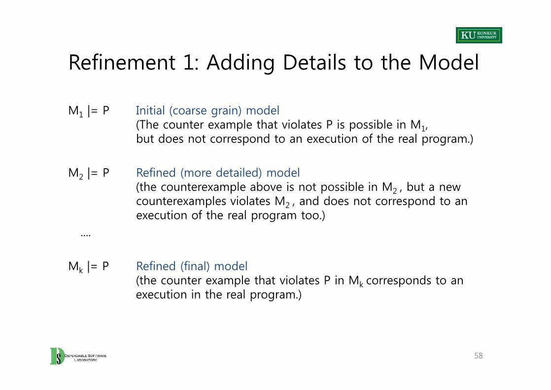
M1 |= P Initial (coarse grain) model(The counter example that violates P is possible in M1, but does not correspond to an execution of the real program.)
M2 |= P Refined (more detailed) model(the counterexample above is not possible in M2 , but a newcounterexamples violates M2 , and does not correspond to anexecution of the real program too.)
....
Mk |= P Refined (final) model(the counter example that violates P in Mk corresponds to anexecution in the real program.)
58
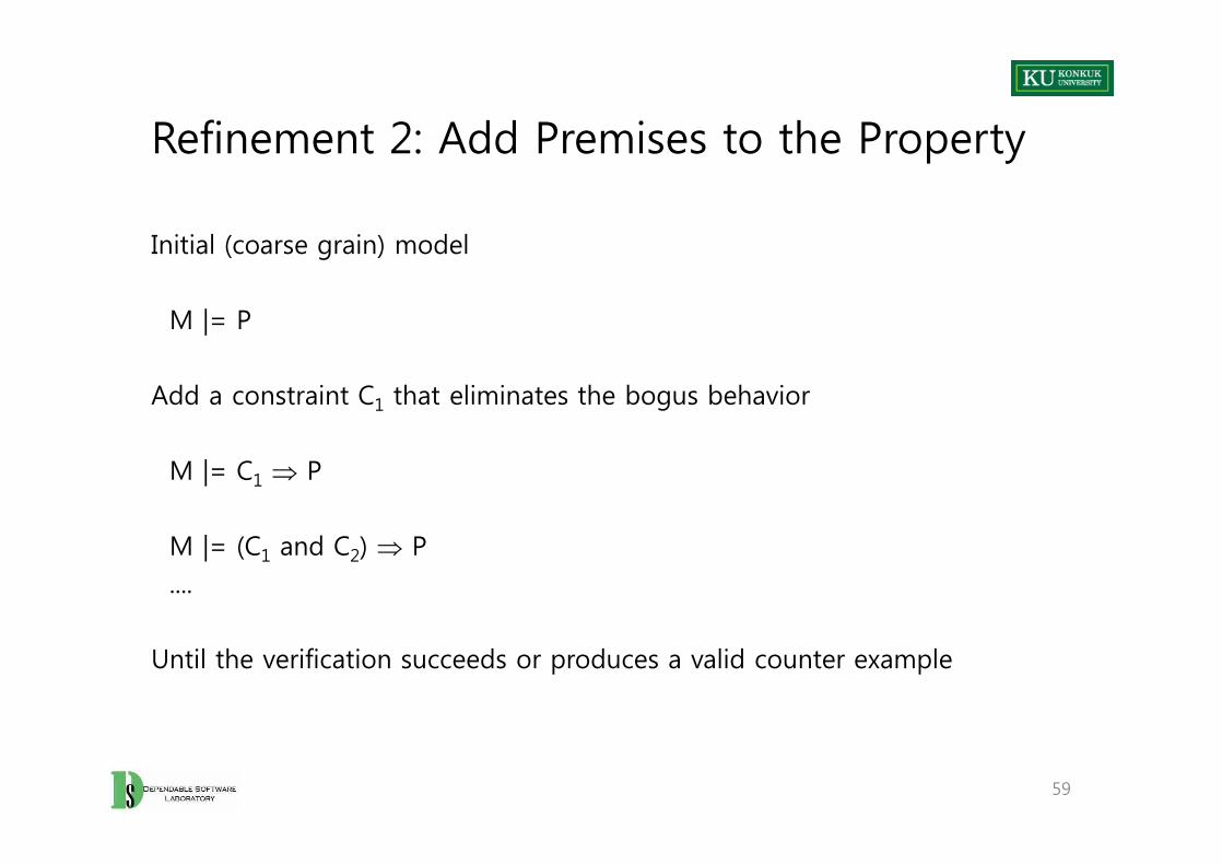
Refinement 2: Add Premises to the Property
Initial (coarse grain) model
M |= P
Add a constraint C1 that eliminates the bogus behavior
M |= C1 Þ P
M |= (C1 and C2) Þ P....
Until the verification succeeds or produces a valid counter example
Initial (coarse grain) model
M |= P
Add a constraint C1 that eliminates the bogus behavior
M |= C1 Þ P
M |= (C1 and C2) Þ P....
Until the verification succeeds or produces a valid counter example
59

60

Part III. Problems and Methods
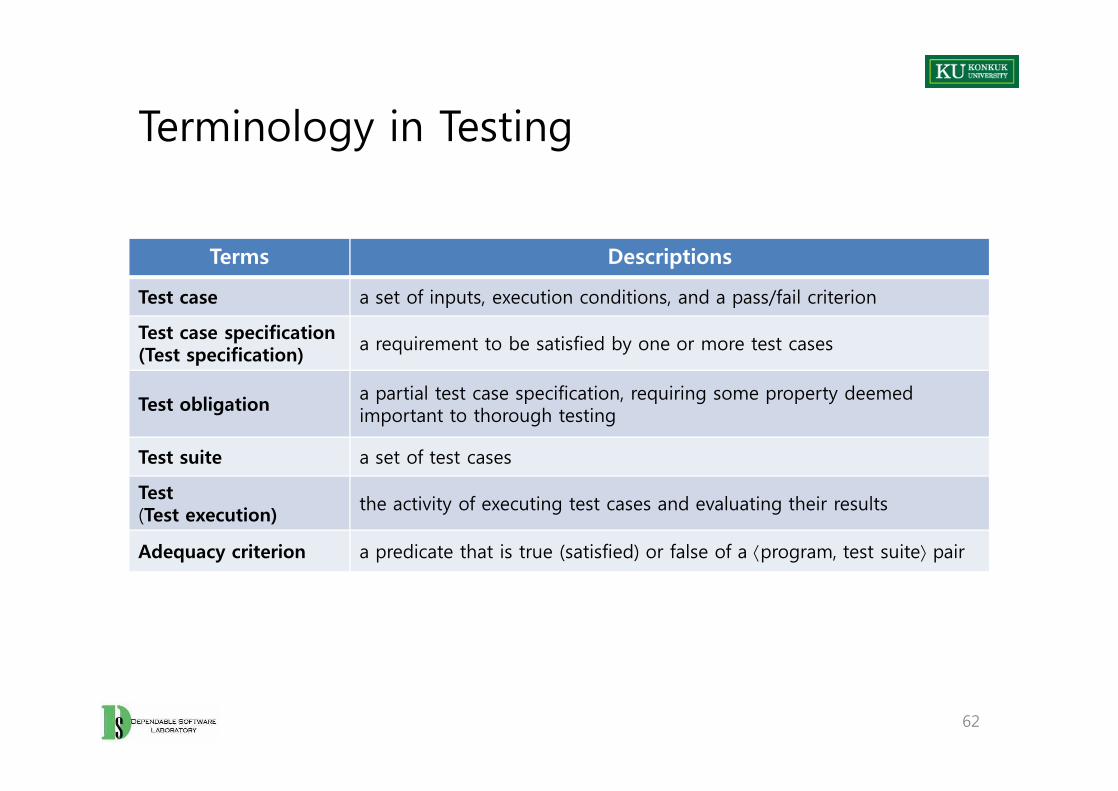
Terminology in Testing
Terms Descriptions
Test case a set of inputs, execution conditions, and a pass/fail criterion
Test case specification (Test specification) a requirement to be satisfied by one or more test cases
Test obligation a partial test case specification, requiring some property deemed important to thorough testing
62
Test obligation a partial test case specification, requiring some property deemed important to thorough testing
Test suite a set of test cases
Test (Test execution) the activity of executing test cases and evaluating their results
Adequacy criterion a predicate that is true (satisfied) or false of a áprogram, test suiteñ pair
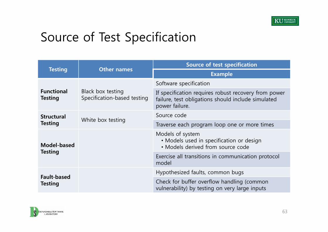
Source of Test Specification
Testing Other namesSource of test specification
Example
Functional Testing
Black box testingSpecification-based testing
Software specification
If specification requires robust recovery from power failure, test obligations should include simulated power failure.
Structural Testing White box testing
Source codeStructural Testing White box testing
Source code
Traverse each program loop one or more times
Model-based Testing
Models of system• Models used in specification or design• Models derived from source code
Exercise all transitions in communication protocol model
Fault-based Testing
Hypothesized faults, common bugs
Check for buffer overflow handling (common vulnerability) by testing on very large inputs
63
Adequacy Criteria
• Adequacy criterion = Set of test obligations
• A test suite satisfies an adequacy criterion, iff– All the tests succeed (pass), and– Every test obligation in the criterion is satisfied by at least one of the test
cases in the test suite.
– Example: • “The statement coverage adequacy criterion is satisfied by test suite S for
program P, if each executable statement in P is executed by at least one test case in S, and the outcome of each test execution was pass.”
64
Coverage
• Measuring coverage (% of satisfied test obligations) can be a useful indicator of – Progress toward a thorough test suite (thoroughness of test suite)
– Trouble spots requiring more attention in testing
• But, coverage is only a proxy for thoroughness or adequacy.– It’s easy to improve coverage without improving a test suite (much easier
than designing good test cases)– The only measure that really matters is (cost-) effectiveness.
65
Comparing Criteria
• Can we distinguish stronger from weaker adequacy criteria?
• Analytical approach– Describe conditions under which one adequacy criterion is provably stronger
than another– Just a piece of the overall “effectiveness” question– Stronger = gives stronger guarantees
→ Subsumes relation
• Can we distinguish stronger from weaker adequacy criteria?
• Analytical approach– Describe conditions under which one adequacy criterion is provably stronger
than another– Just a piece of the overall “effectiveness” question– Stronger = gives stronger guarantees
→ Subsumes relation
66
Subsumes Relation
• Test adequacy criterion A subsumes test adequacy criterion B iff, for every program P, every test suite satisfying A with respect to P also satisfies B with respect to P.
– E.g. Exercising all program branches (branch coverage) subsumes exercising all program statements.
• A common analytical comparison of closely related criteria– Useful for working from easier to harder levels of coverage, but not a direct
indication of quality
67
68
Functional Testing
• Functional testing– Deriving test cases from program specifications – ‘Functional’ refers to the source of information used in test case design, not
to what is tested.
• Also known as:– Specification-based testing (from specifications)– Black-box testing (no view of source code)
• Functional specification = description of intended program behavior– Formal or informal
69
Systematic testing vs. Random testing
• Random (uniform) testing– Pick possible inputs uniformly– Avoids designer’s bias– But, treats all inputs as equally valuable
• Systematic (non-uniform) testing– Try to select inputs that are especially valuable– Usually by choosing representatives of classes that are apt to fail often or not
at all
• Functional testing is a systematic (partition-based) testing strategy.
70
Purpose of Testing
• Our goal is to find needles and remove them from hay. → Look systematically (non-uniformly) for needles !!!– We need to use everything we know about needles.
• E.g. Are they heavier than hay? Do they sift to the bottom?
• To estimate the proportion of needles to hay → Sample randomly !!!– Reliability estimation requires unbiased samples for valid statistics. – But that’s not our goal.
71
Systematic Partition Testing
Failure (valuable test case)
No failure
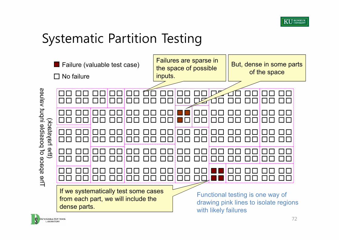
Failures are sparse in the space of possible inputs.
But, dense in some parts of the space
The space of possible input values
(the haystack)
72
If we systematically test some cases from each part, we will include the dense parts.
Functional testing is one way of drawing pink lines to isolate regions with likely failures
The space of possible input values
(the haystack)
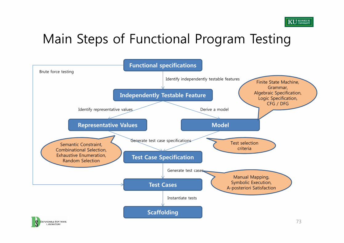
Main Steps of Functional Program Testing
Functional specifications
Independently Testable Feature
Representative Values Model
Identify independently testable features
Derive a modelIdentify representative values
Finite State Machine,Grammar,
Algebraic Specification,Logic Specification,
CFG / DFG
Brute force testing
73
Representative Values Model
Test Case Specification
Test Cases
Scaffolding
Generate test case specifications
Generate test cases
Instantiate tests
Test selection criteria
Manual Mapping,Symbolic Execution,
A-posteriori Satisfaction
Semantic Constraint,Combinational Selection,Exhaustive Enumeration,
Random Selection
Key Ideas in Combinatorial Approaches
1. Category-partition testing– Separate (manual) identification of values that characterize the input space
from (automatic) generation of combinations for test cases
2. Pairwise testing – Systematically test interactions among attributes of the program input space
with a relatively small number of test cases
3. Catalog-based testing– Aggregate and synthesize the experience of test designers in a particular
organization or application domain, to aid in identifying attribute values
74
1. Category-Partition Testing
1. Decompose the specification into independently testable features– for each feature, identify parameters and environment elements– for each parameter and environment element, identify elementary
characteristics (→ categories)
2. Identify representative values– for each characteristic(category), identify classes of values
• normal values• boundary values• special values• error values
3. Generate test case specifications
75
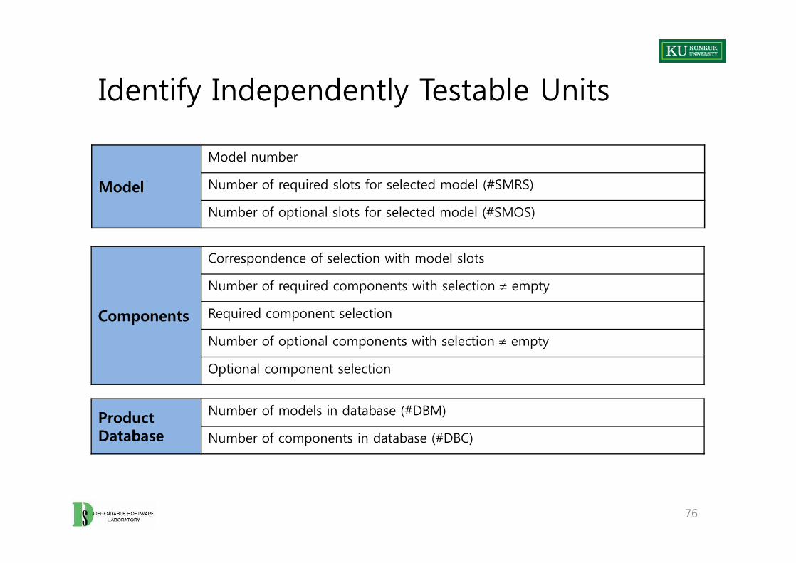
Identify Independently Testable Units
Model
Model number
Number of required slots for selected model (#SMRS)
Number of optional slots for selected model (#SMOS)
Correspondence of selection with model slots
Number of required components with selection ¹ empty
76
Components
Number of required components with selection ¹ empty
Required component selection
Number of optional components with selection ¹ empty
Optional component selection
Product Database
Number of models in database (#DBM)
Number of components in database (#DBC)
Step 2: Identify Representative Values
• Identify representative classes of values for each of the categories
• Representative values may be identified by applying – Boundary value testing
• Select extreme values within a class • Select values outside but as close as possible to the class• Select interior (non-extreme) values of the class
– Erroneous condition testing• Select values outside the normal domain of the program
77
Representative Values: Model
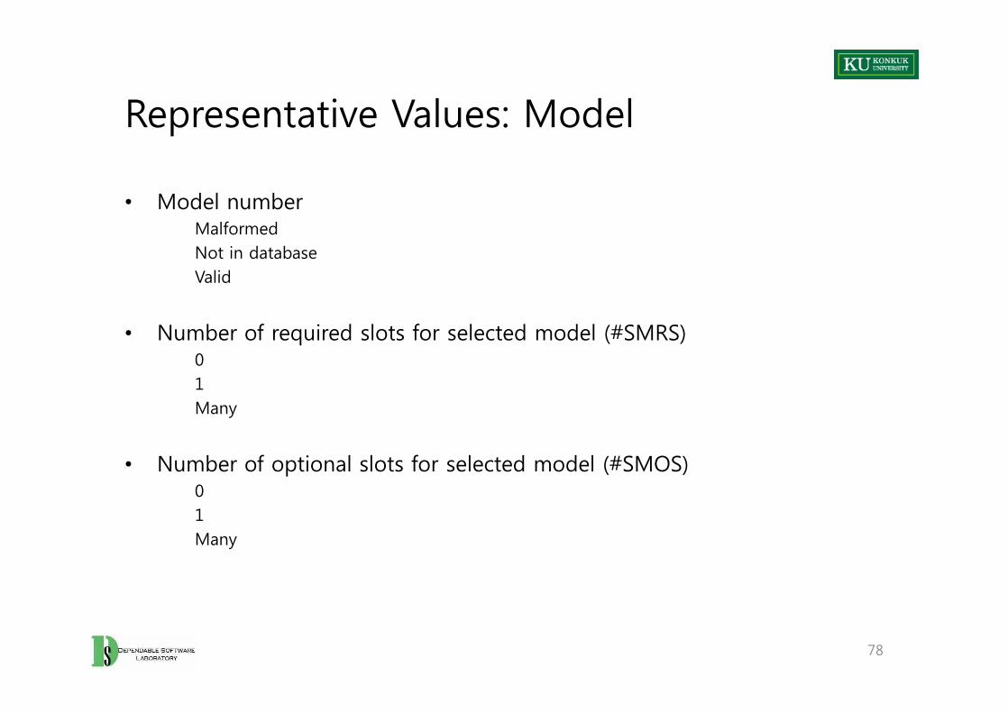
• Model numberMalformedNot in databaseValid
• Number of required slots for selected model (#SMRS)01Many
• Number of optional slots for selected model (#SMOS)01Many
• Model numberMalformedNot in databaseValid
• Number of required slots for selected model (#SMRS)01Many
• Number of optional slots for selected model (#SMOS)01Many
78
Step 3: Generate Test Case Specifications
• A combination of values for each category corresponds to a test case specification.
– In the example, we have 314,928 test cases.– Most of which are impossible.– Example: zero slots and at least one incompatible slot
• Need to introduce constraints in order to– Rule out impossible combinations, and– Reduce the size of the test suite, if too large
– Example:• Error constraints• Property constraints• Single constraints
79
Error Constraints
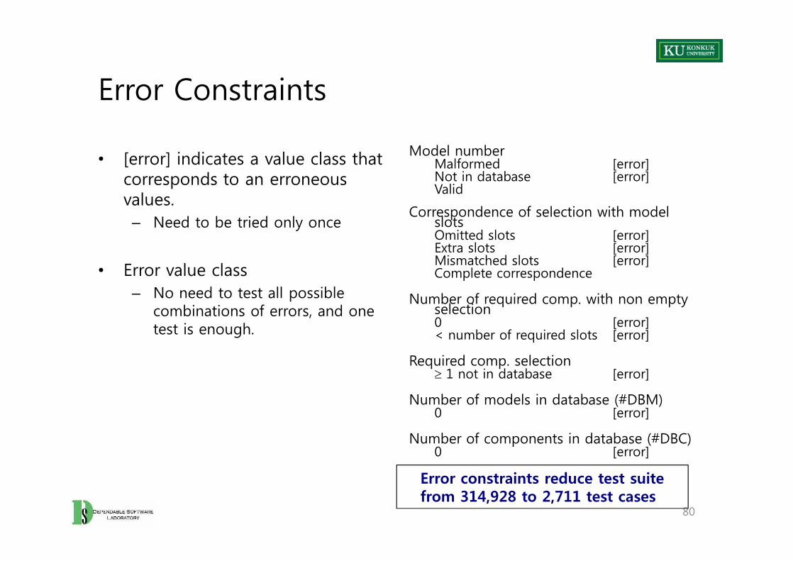
• [error] indicates a value class that corresponds to an erroneous values.
– Need to be tried only once
• Error value class– No need to test all possible
combinations of errors, and one test is enough.
Model numberMalformed [error]Not in database [error]Valid
Correspondence of selection with model slotsOmitted slots [error]Extra slots [error]Mismatched slots [error]Complete correspondence
Number of required comp. with non empty selection0 [error]< number of required slots [error]
Required comp. selection³ 1 not in database [error]
Number of models in database (#DBM)0 [error]
Number of components in database (#DBC)0 [error]
80
Error constraints reduce test suite from 314,928 to 2,711 test cases
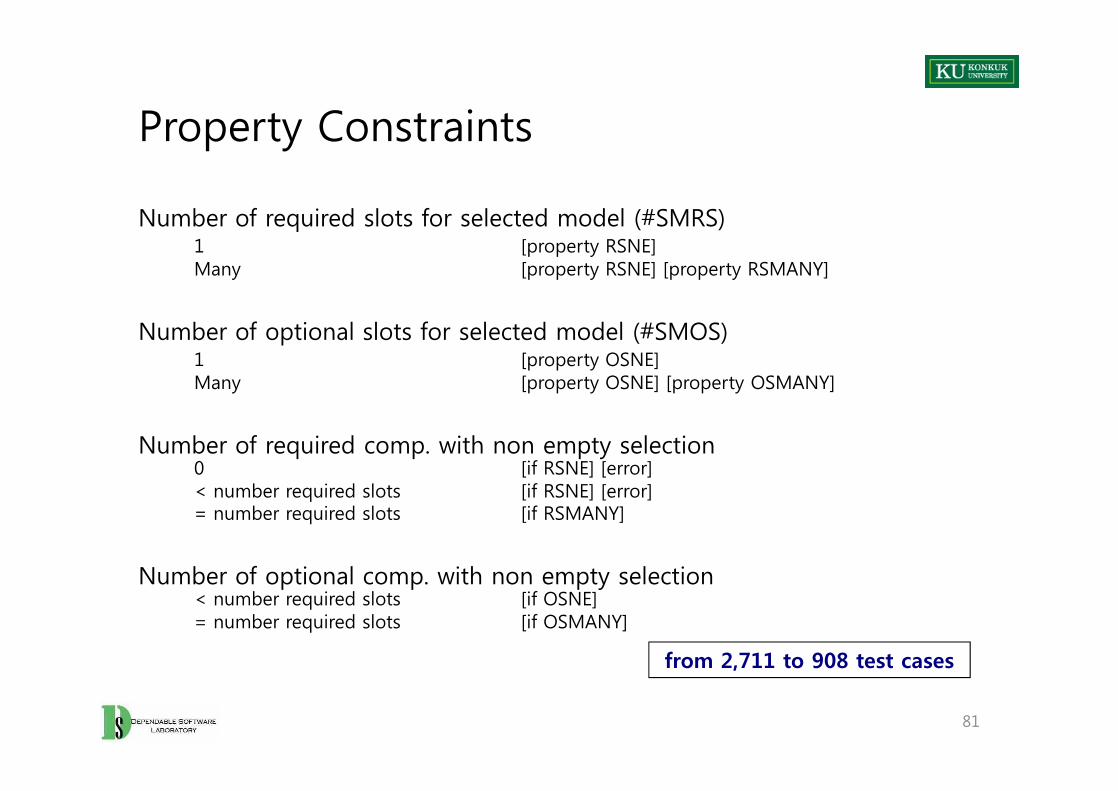
Property Constraints
Number of required slots for selected model (#SMRS)1 [property RSNE]Many [property RSNE] [property RSMANY]
Number of optional slots for selected model (#SMOS)1 [property OSNE]Many [property OSNE] [property OSMANY]
Number of required comp. with non empty selection0 [if RSNE] [error]< number required slots [if RSNE] [error]= number required slots [if RSMANY]
Number of optional comp. with non empty selection< number required slots [if OSNE]= number required slots [if OSMANY]
81
from 2,711 to 908 test cases
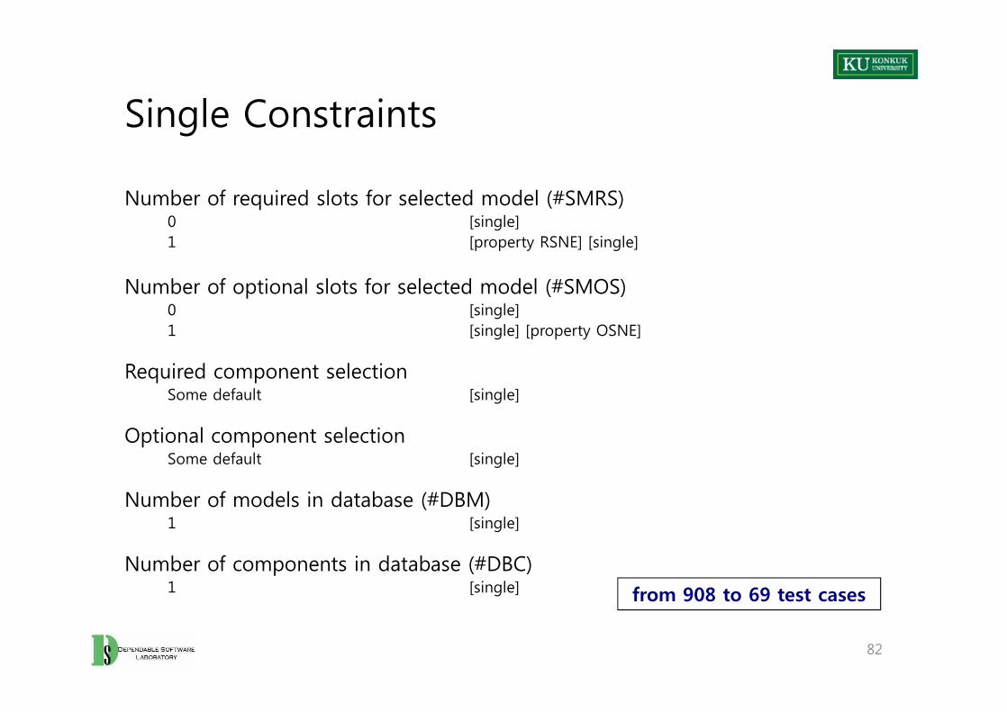
Single Constraints
Number of required slots for selected model (#SMRS)0 [single]1 [property RSNE] [single]
Number of optional slots for selected model (#SMOS)0 [single]1 [single] [property OSNE]
Required component selectionSome default [single]
Optional component selectionSome default [single]
Number of models in database (#DBM)1 [single]
Number of components in database (#DBC)1 [single]
82
from 908 to 69 test cases
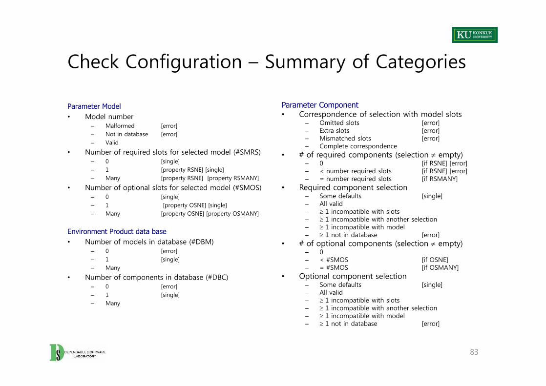
Check Configuration – Summary of Categories
Parameter Model• Model number
– Malformed [error]– Not in database [error]– Valid
• Number of required slots for selected model (#SMRS)– 0 [single]– 1 [property RSNE] [single] – Many [property RSNE] [property RSMANY]
• Number of optional slots for selected model (#SMOS)– 0 [single]– 1 [property OSNE] [single] – Many [property OSNE] [property OSMANY]
Environment Product data base• Number of models in database (#DBM)
– 0 [error]– 1 [single]– Many
• Number of components in database (#DBC)– 0 [error]– 1 [single]– Many
Parameter Component• Correspondence of selection with model slots
– Omitted slots [error]– Extra slots [error]– Mismatched slots [error]– Complete correspondence
• # of required components (selection ¹ empty)– 0 [if RSNE] [error]– < number required slots [if RSNE] [error]– = number required slots [if RSMANY]
• Required component selection– Some defaults [single]– All valid– ³ 1 incompatible with slots– ³ 1 incompatible with another selection– ³ 1 incompatible with model– ³ 1 not in database [error]
• # of optional components (selection ¹ empty)– 0– < #SMOS [if OSNE]– = #SMOS [if OSMANY]
• Optional component selection– Some defaults [single]– All valid– ³ 1 incompatible with slots– ³ 1 incompatible with another selection– ³ 1 incompatible with model– ³ 1 not in database [error]
83
2. Pairwise Combination Testing
• Category partition works well when intuitive constraints reduce the number of combinations to a small amount of test cases.
– Without many constraints, the number of combinations may be unmanageable.
• Pairwise combination– Instead of exhaustive combinations– Generate combinations that efficiently cover all pairs (triples,…) of classes– Rationale:
• Most failures are triggered by single values or combinations of a few values.• Covering pairs (triples,…) reduces the number of test cases, but reveals most faults.
84
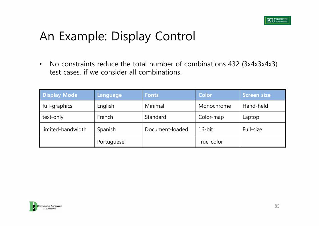
An Example: Display Control
• No constraints reduce the total number of combinations 432 (3x4x3x4x3) test cases, if we consider all combinations.
Display Mode Language Fonts Color Screen size
full-graphics English Minimal Monochrome Hand-held
text-only French Standard Color-map Laptop
85
text-only French Standard Color-map Laptop
limited-bandwidth Spanish Document-loaded 16-bit Full-size
Portuguese True-color
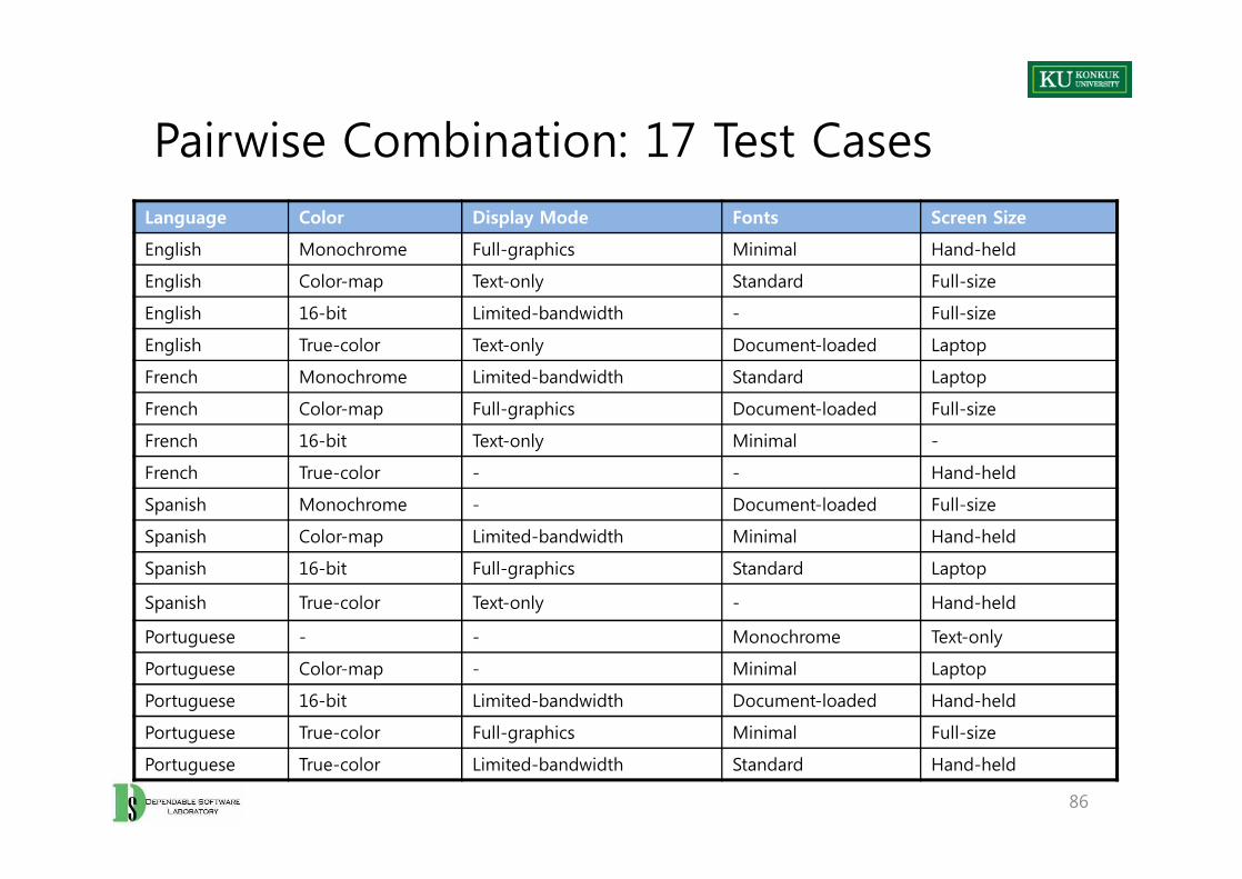
Pairwise Combination: 17 Test CasesLanguage Color Display Mode Fonts Screen Size
English Monochrome Full-graphics Minimal Hand-held
English Color-map Text-only Standard Full-size
English 16-bit Limited-bandwidth - Full-size
English True-color Text-only Document-loaded Laptop
French Monochrome Limited-bandwidth Standard Laptop
French Color-map Full-graphics Document-loaded Full-size
French 16-bit Text-only Minimal -
86
French 16-bit Text-only Minimal -
French True-color - - Hand-held
Spanish Monochrome - Document-loaded Full-size
Spanish Color-map Limited-bandwidth Minimal Hand-held
Spanish 16-bit Full-graphics Standard Laptop
Spanish True-color Text-only - Hand-held
Portuguese - - Monochrome Text-only
Portuguese Color-map - Minimal Laptop
Portuguese 16-bit Limited-bandwidth Document-loaded Hand-held
Portuguese True-color Full-graphics Minimal Full-size
Portuguese True-color Limited-bandwidth Standard Hand-held
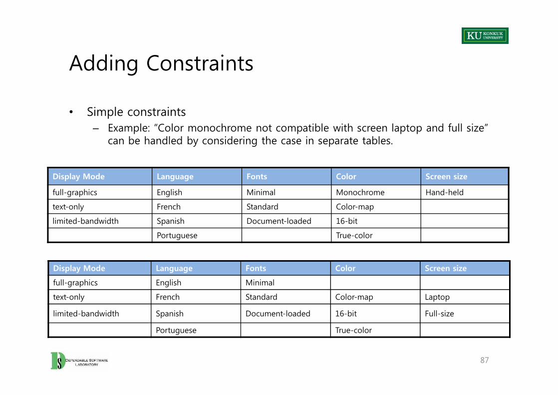
Adding Constraints
• Simple constraints– Example: “Color monochrome not compatible with screen laptop and full size”
can be handled by considering the case in separate tables.
Display Mode Language Fonts Color Screen size
full-graphics English Minimal Monochrome Hand-held
87
text-only French Standard Color-map
limited-bandwidth Spanish Document-loaded 16-bit
Portuguese True-color
Display Mode Language Fonts Color Screen size
full-graphics English Minimal
text-only French Standard Color-map Laptop
limited-bandwidth Spanish Document-loaded 16-bit Full-size
Portuguese True-color
Structural Testing
• Judging test suite thoroughness based on the structure of the programitself
– Also known as • White-box testing• Glass-box testing • Code-based testing
– Distinguish from functional (requirements-based, “black-box”) testing
• Structural testing is still testing product functionality against its specification.
– Only the measure of thoroughness has changed.
88
Rationale of Structural Testing
• One way of answering the question “What is missing in our test suite?”– If a part of a program is not executed by any test case in the suite, faults in
that part cannot be exposed.– But what’s the ‘part’?
• Typically, a control flow element or combination• Statements (or CFG nodes), Branches (or CFG edges)• Fragments and combinations: Conditions, paths
• Structural testing complements functional testing.– Another way to recognize cases that are treated differently
• Recalling fundamental rationale– Prefer test cases that are treated differently over cases treated the same
89
No Guarantee
• Executing all control flow elements does not guarantee finding all faults.– Execution of a faulty statement may not always result in a failure.
• The state may not be corrupted when the statement is executed with some data values.
• Corrupt state may not propagate through execution to eventually lead to failure.
• What is the value of structural coverage?– Increases confidence in thoroughness of testing
90
Structural Testing Complements Functional Testing
• Control flow-based testing includes cases that may not be identified from specifications alone.
– Typical case: Implementation of a single item of the specification by multiple parts of the program
– E.g. Hash table collision (invisible in interface specification)
• Test suites that satisfy control flow adequacy criteria could fail in revealing faults that can be caught with functional criteria.
– Typical case: Missing path faults
91
Structural Testing, in Practice
• Create functional test suite first, then measure structural coverage to identify and see what is missing.
• Interpret unexecuted elements– May be due to natural differences between specification and implementation– May reveal flaws of the software or its development process
• Inadequacy of specifications that do not include cases present in the implementation
• Coding practice that radically diverges from the specification• Inadequate functional test suites
• Attractive because structural testing is automated– Coverage measurements are convenient progress indicators.– Sometimes used as a criterion of completion of testing
• Use with caution: does not ensure effective test suites
92
An Example Program: ‘cgi_decode’ and CFG
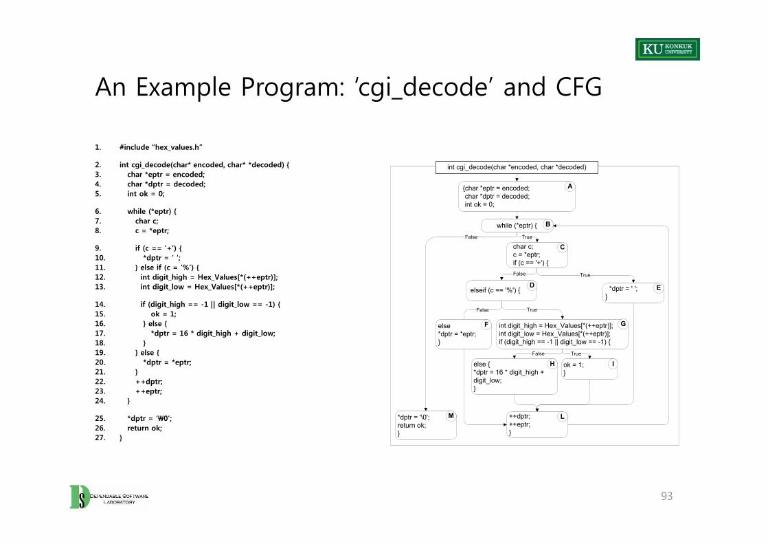
1. #include “hex_values.h”
2. int cgi_decode(char* encoded, char* *decoded) {3. char *eptr = encoded;4. char *dptr = decoded;5. int ok = 0;
6. while (*eptr) {7. char c;8. c = *eptr;
9. if (c == ‘+’) {10. *dptr = ‘ ‘;11. } else if (c = ‘%’) {12. int digit_high = Hex_Values[*(++eptr)];13. int digit_low = Hex_Values[*(++eptr)];
14. if (digit_high == -1 || digit_low == -1) {15. ok = 1;16. } else {17. *dptr = 16 * digit_high + digit_low;18. }19. } else {20. *dptr = *eptr;21. }22. ++dptr;23. ++eptr;24. }
25. *dptr = ‘\0’;26. return ok;27. }
{char *eptr = encoded;char *dptr = decoded;int ok = 0;
char c;c = *eptr;if (c == '+') {
while (*eptr) {TrueFalse
int cgi_decode(char *encoded, char *decoded)
A
C
B
1. #include “hex_values.h”
2. int cgi_decode(char* encoded, char* *decoded) {3. char *eptr = encoded;4. char *dptr = decoded;5. int ok = 0;
6. while (*eptr) {7. char c;8. c = *eptr;
9. if (c == ‘+’) {10. *dptr = ‘ ‘;11. } else if (c = ‘%’) {12. int digit_high = Hex_Values[*(++eptr)];13. int digit_low = Hex_Values[*(++eptr)];
14. if (digit_high == -1 || digit_low == -1) {15. ok = 1;16. } else {17. *dptr = 16 * digit_high + digit_low;18. }19. } else {20. *dptr = *eptr;21. }22. ++dptr;23. ++eptr;24. }
25. *dptr = ‘\0’;26. return ok;27. }
93
*dptr = ' ';}
*dptr = '\0';return ok;}
True
int digit_high = Hex_Values[*(++eptr)];int digit_low = Hex_Values[*(++eptr)];if (digit_high == -1 || digit_low == -1) {
True
ok = 1;}
True
else {*dptr = 16 * digit_high + digit_low;}
False
++dptr;++eptr;}
False
False
elseif (c == '%') {
else*dptr = *eptr;}
D E
F G
H I
LM
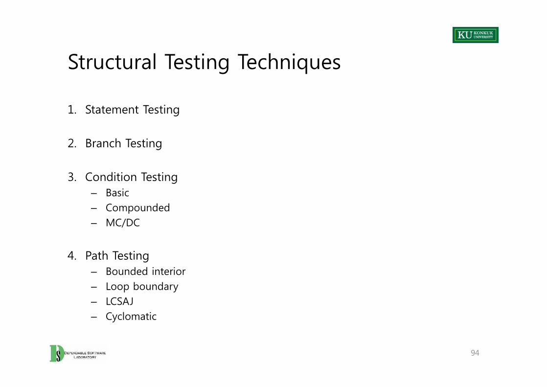
Structural Testing Techniques
1. Statement Testing
2. Branch Testing
3. Condition Testing– Basic– Compounded– MC/DC
4. Path Testing– Bounded interior– Loop boundary– LCSAJ– Cyclomatic
1. Statement Testing
2. Branch Testing
3. Condition Testing– Basic– Compounded– MC/DC
4. Path Testing– Bounded interior– Loop boundary– LCSAJ– Cyclomatic
94
1. Statement Testing
• Adequacy criterion: – Each statement (or node in the CFG) must be executed at least once.
• Coverage:number of executed statements
number of statements
• Rationale: – A fault in a statement can only be revealed by executing the faulty statement.
• Nodes in a CFG often represent basic blocks of multiple statements.– Some standards refer to ‘basic block coverage’ or ‘node coverage’.– Difference in granularity, but not in concept
95
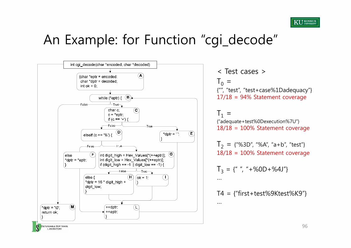
An Example: for Function “cgi_decode”
< Test cases >T0 = {“”, “test”, “test+case%1Dadequacy”}17/18 = 94% Statement coverage
T1 = {“adequate+test%0Dexecution%7U”}18/18 = 100% Statement coverage
T2 = {“%3D”, “%A”, “a+b”, “test”}18/18 = 100% Statement coverage
T3 = {“ ”, “+%0D+%4J”}…
T4 = {“first+test%9Ktest%K9”}…
96
< Test cases >T0 = {“”, “test”, “test+case%1Dadequacy”}17/18 = 94% Statement coverage
T1 = {“adequate+test%0Dexecution%7U”}18/18 = 100% Statement coverage
T2 = {“%3D”, “%A”, “a+b”, “test”}18/18 = 100% Statement coverage
T3 = {“ ”, “+%0D+%4J”}…
T4 = {“first+test%9Ktest%K9”}…
Coverage is not a Matter of Size
• Coverage does not depend on the number of test cases.– T0 , T1 : T1 >coverage T0 T1 <cardinality T0
– T1 , T2 : T2 =coverage T1 T2 >cardinality T1
• Minimizing test suite size is not the goal.– Small test cases make failure diagnosis easier.– But, a failing test case in T2 gives more information for fault localization than
a failing test case in T1
97
Complete Statement Coverage
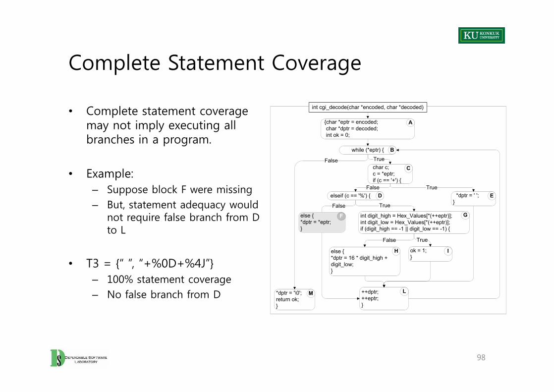
• Complete statement coverage may not imply executing all branches in a program.
• Example: – Suppose block F were missing– But, statement adequacy would
not require false branch from D to L
• T3 = {“ ”, “+%0D+%4J”}– 100% statement coverage– No false branch from D
{char *eptr = encoded;char *dptr = decoded;int ok = 0;
char c;c = *eptr;if (c == '+') {
*dptr = ' ';
while (*eptr) {
TrueFalse
TrueFalse elseif (c == '%') {
int cgi_decode(char *encoded, char *decoded)
A
C
B
D E
• Complete statement coverage may not imply executing all branches in a program.
• Example: – Suppose block F were missing– But, statement adequacy would
not require false branch from D to L
• T3 = {“ ”, “+%0D+%4J”}– 100% statement coverage– No false branch from D
98
dptr = ' ';}
*dptr = '\0';return ok;}
int digit_high = Hex_Values[*(++eptr)];int digit_low = Hex_Values[*(++eptr)];if (digit_high == -1 || digit_low == -1) {
True
ok = 1;}
True
else {*dptr = 16 * digit_high + digit_low;}
False
++dptr;++eptr;}
False
elseif (c == % ) {
else {*dptr = *eptr;}
D E
F G
H I
LM
2. Branch Testing
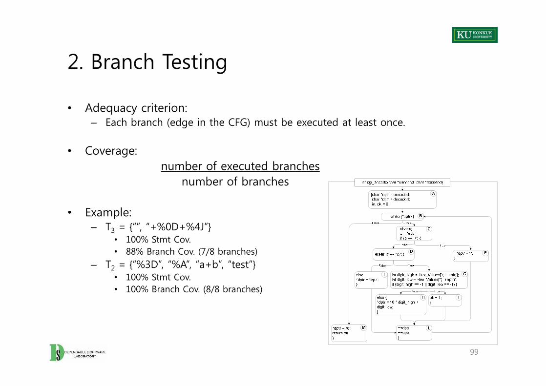
• Adequacy criterion: – Each branch (edge in the CFG) must be executed at least once.
• Coverage:number of executed branches
number of branches
• Example:– T3 = {“”, “+%0D+%4J”}
• 100% Stmt Cov.• 88% Branch Cov. (7/8 branches)
– T2 = {“%3D”, “%A”, “a+b”, “test”}• 100% Stmt Cov. • 100% Branch Cov. (8/8 branches)
99
Statements vs. Branches
• Traversing all edges causes all nodes to be visited.– Therefore, test suites that satisfy the branch adequacy also satisfy the
statement adequacy criterion for the same program.– Branch adequacy subsumes statement adequacy.
• The converse is not true (see T3)– A statement-adequate test suite may not be branch-adequate.
100
All Branches Coverage
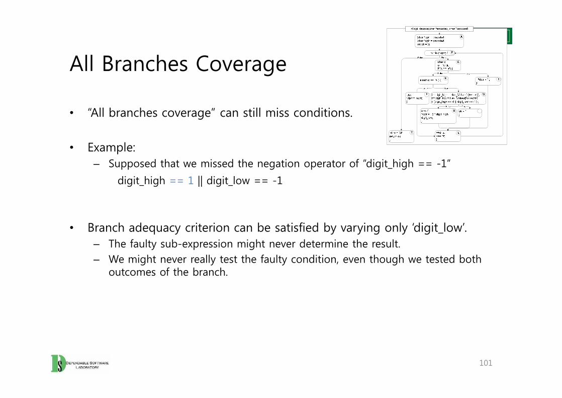
• “All branches coverage” can still miss conditions.
• Example: – Supposed that we missed the negation operator of “digit_high == -1”
digit_high == 1 || digit_low == -1
• Branch adequacy criterion can be satisfied by varying only ‘digit_low’.– The faulty sub-expression might never determine the result.– We might never really test the faulty condition, even though we tested both
outcomes of the branch.
101
3. Condition Testing
• Branch coverage exposes faults in how a computation has been decomposed into cases.
– Intuitively attractive: checking the programmer’s case analysis– But, only roughly: grouping cases with the same outcome
• Condition coverage considers case analysis in more detail.– Consider ‘individual conditions’ in a compound Boolean expression
• E.g. both parts of ‘”igit_high == 1 || digit_low == -1”
• Adequacy criterion: – Each basic condition must be executed at least once.
• Basic condition testing coverage:number of truth values taken by all basic conditions
2 * number of basic conditions
102
Basic Conditions vs. Branches
• Basic condition adequacy criterion can be satisfied without satisfying branch coverage.
• T4 = {“first+test%9Ktest%K9”}– Satisfies basic condition adequacy– But, does not satisfy branch condition adequacy
• Branch and basic condition are not comparable. – Neither implies the other.
• Basic condition adequacy criterion can be satisfied without satisfying branch coverage.
• T4 = {“first+test%9Ktest%K9”}– Satisfies basic condition adequacy– But, does not satisfy branch condition adequacy
• Branch and basic condition are not comparable. – Neither implies the other.
103
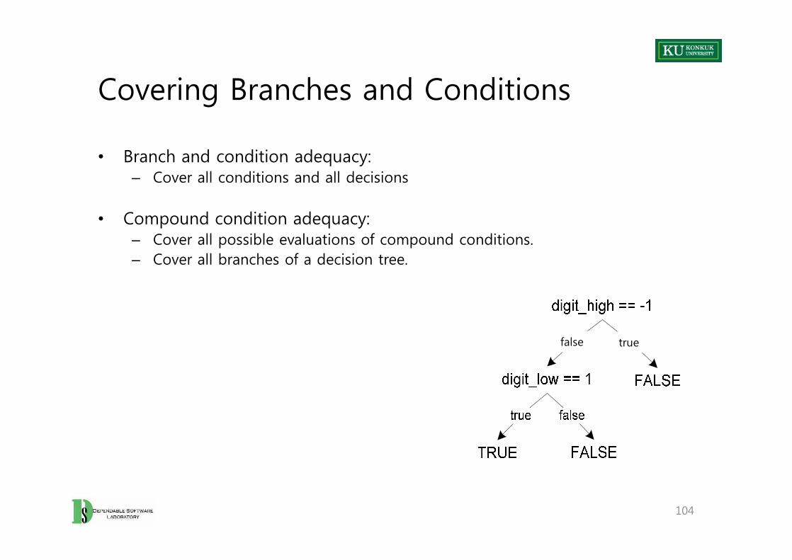
Covering Branches and Conditions
• Branch and condition adequacy: – Cover all conditions and all decisions
• Compound condition adequacy:– Cover all possible evaluations of compound conditions.– Cover all branches of a decision tree.
• Branch and condition adequacy: – Cover all conditions and all decisions
• Compound condition adequacy:– Cover all possible evaluations of compound conditions.– Cover all branches of a decision tree.
104
truefalse
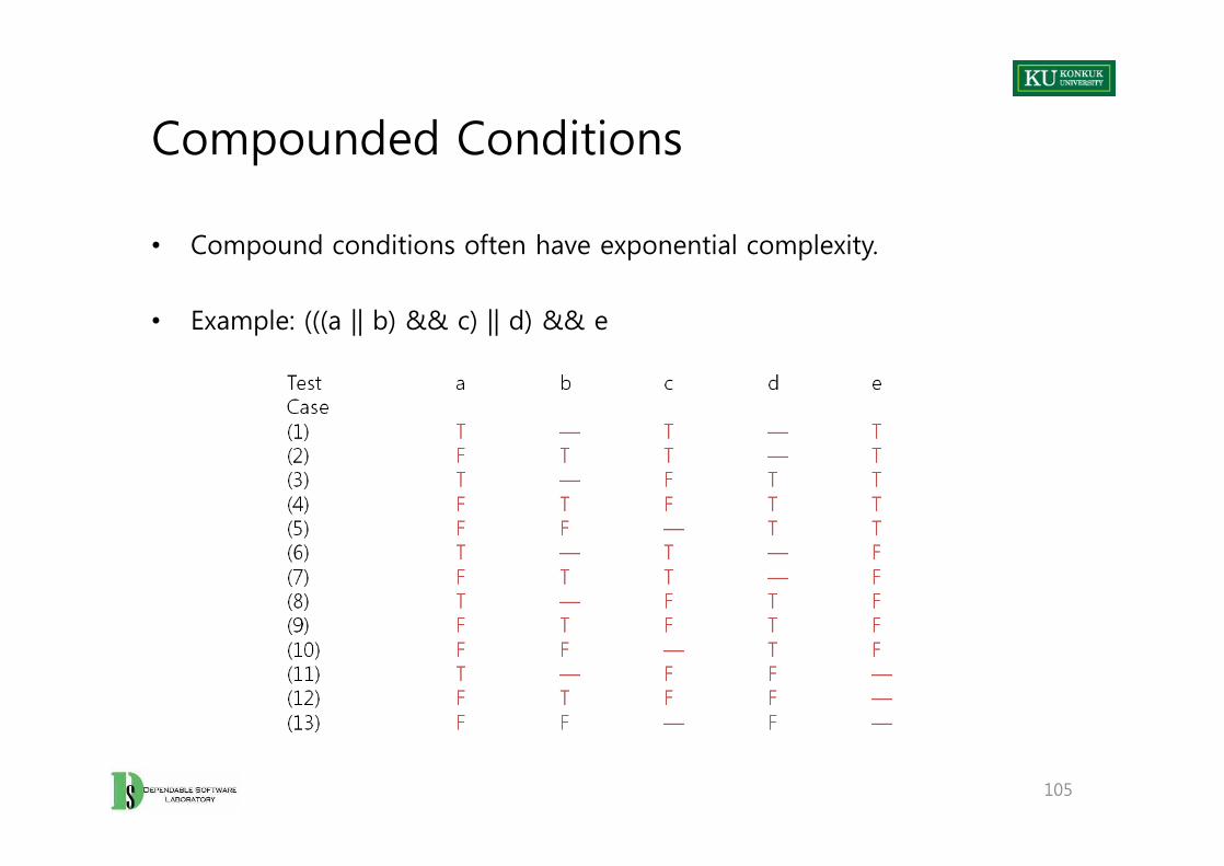
Compounded Conditions
• Compound conditions often have exponential complexity.
• Example: (((a || b) && c) || d) && e
105

Modified Condition/Decision (MC/DC)
• Motivation– Effectively test important combinations of conditions, without exponential
blowup in test suite size – “Important” combinations means:
• Each basic condition shown to independently affect the outcome of each decision
• Requires– For each basic condition C, two test cases,– Values of all ‘evaluated’ conditions except C are the same.– Compound condition as a whole evaluates to ‘true’ for one and ‘false’ for the
other.
106
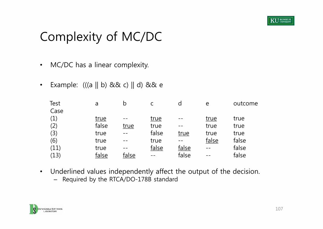
Complexity of MC/DC
• MC/DC has a linear complexity.
• Example: (((a || b) && c) || d) && e
Test a b c d e outcomeCase(1) true -- true -- true true(2) false true true -- true true(3) true -- false true true true(6) true -- true -- false false(11) true -- false false -- false(13) false false -- false -- false
• Underlined values independently affect the output of the decision.– Required by the RTCA/DO-178B standard
107
Comments on MC/DC
• MC/DC is – Basic condition coverage (C)– Branch coverage (DC)– Plus one additional condition (M)
• Every condition must independently affect the decision’s output.
• It is subsumed by compound conditions and subsumes all other criteria discussed so far.
– Stronger than statement and branch coverage
• A good balance of thoroughness and test size – Widely used
108
4. Path Testing
• There are many more paths than branches.– Decision and condition adequacy criteria consider individual decisions only.
• Path testing focuses combinations of decisions along paths.
• Adequacy criterion: – Each path must be executed at least once.
• Coverage:number of executed paths
number of paths
109
Path Coverage Criteria in Practice
• The number of paths in a program with loops is unbounded. – Usually impossible to satisfy
• For a feasible criterion, – Should partition infinite set of paths into a finite number of classes
• Useful criteria can be obtained by limiting – Number of traversals of loops– Length of the paths to be traversed– Dependencies among selected paths
110
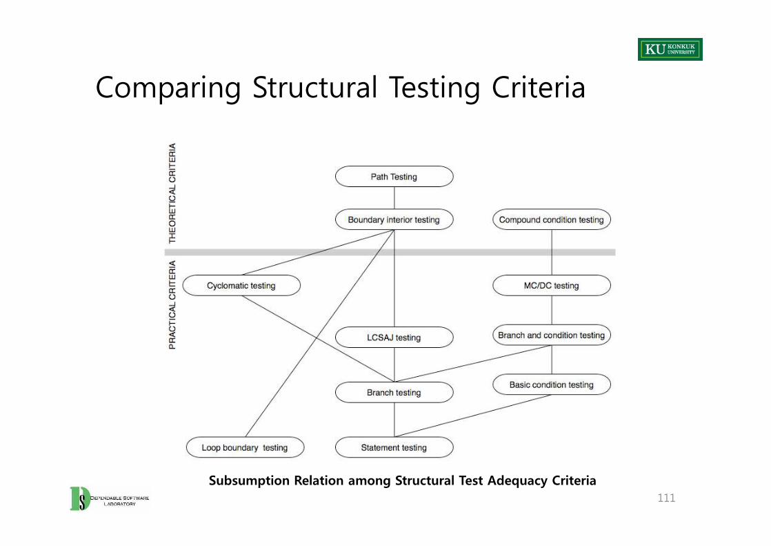
Comparing Structural Testing Criteria
111
Subsumption Relation among Structural Test Adequacy Criteria
Motivation
• Middle ground in structural testing– Node and edge coverage don’t test interactions.– Path-based criteria require impractical number of test cases.
• Only a few paths uncover additional faults, anyway.
– Need to distinguish “important” paths
• Intuition: Statements interact through data flow.– Value computed in one statement, is used in another.– Bad value computation can be revealed only when it is used.
112
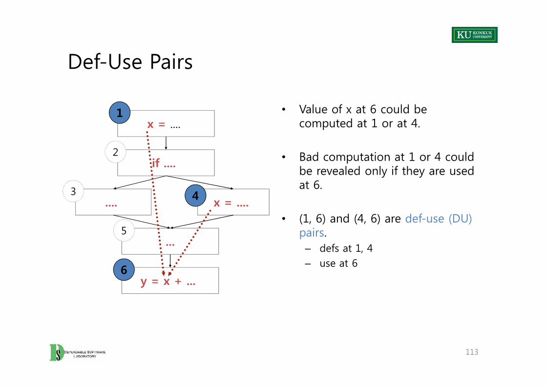
Def-Use Pairs
• Value of x at 6 could be computed at 1 or at 4.
• Bad computation at 1 or 4 could be revealed only if they are used at 6.
• (1, 6) and (4, 6) are def-use (DU) pairs.
– defs at 1, 4– use at 6
x = ....
if ....
x = .... .... 4
1
2
3
• Value of x at 6 could be computed at 1 or at 4.
• Bad computation at 1 or 4 could be revealed only if they are used at 6.
• (1, 6) and (4, 6) are def-use (DU) pairs.
– defs at 1, 4– use at 6
113
x = ....
...
....
y = x + ...
4
6
3
5
Terminology
• DU pair– A pair of definition and use for some variable, such that at least one DU path
exists from the definition to the use.– “x = ...” is a definition of x– “= ... x ...” is a use of x
• DU path – A definition-clear path on the CFG starting from a definition to a use of a
same variable– Definition clear: Value is not replaced on path.– Note: Loops could create infinite DU paths between a def and a use.
114
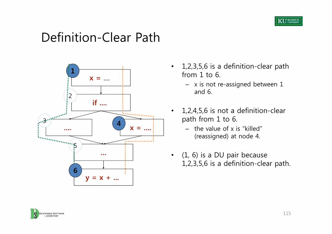
Definition-Clear Path
• 1,2,3,5,6 is a definition-clear path from 1 to 6.
– x is not re-assigned between 1 and 6.
• 1,2,4,5,6 is not a definition-clear path from 1 to 6.
– the value of x is “killed” (reassigned) at node 4.
• (1, 6) is a DU pair because 1,2,3,5,6 is a definition-clear path.
x = ....
if ....
4
1
2
3
• 1,2,3,5,6 is a definition-clear path from 1 to 6.
– x is not re-assigned between 1 and 6.
• 1,2,4,5,6 is not a definition-clear path from 1 to 6.
– the value of x is “killed” (reassigned) at node 4.
• (1, 6) is a DU pair because 1,2,3,5,6 is a definition-clear path.
115
x = ....
...
....
y = x + ...
4
6
3
5
Adequacy Criteria
• All DU pairs – Each DU pair is exercised by at least one test case.
• All DU paths – Each simple (non looping) DU path is exercised by at least one test case.
• All definitions– For each definition, there is at least one test case which exercises a DU pair
containing it.– Because, every computed value is used somewhere.
• Corresponding coverage fractions can be defined similarly.
116
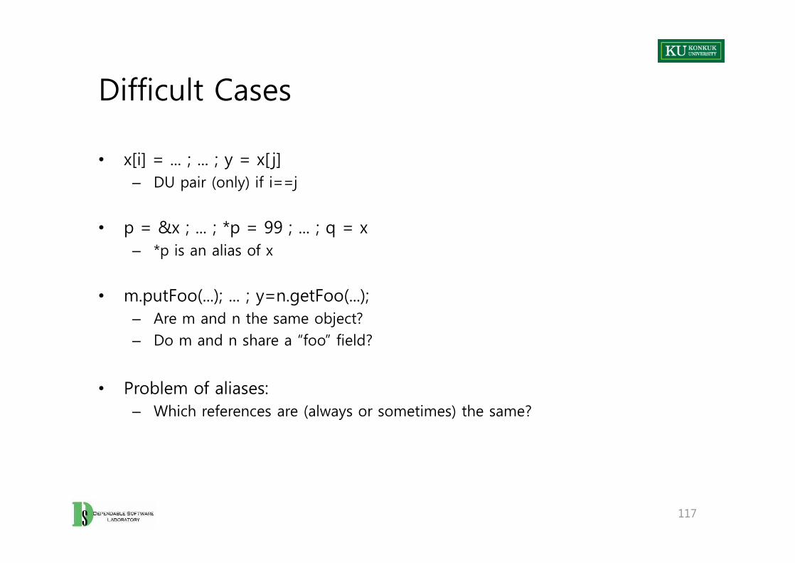
Difficult Cases
• x[i] = ... ; ... ; y = x[ j]– DU pair (only) if i==j
• p = &x ; ... ; *p = 99 ; ... ; q = x– *p is an alias of x
• m.putFoo(...); ... ; y=n.getFoo(...); – Are m and n the same object?– Do m and n share a “foo” field?
• Problem of aliases: – Which references are (always or sometimes) the same?
• x[i] = ... ; ... ; y = x[ j]– DU pair (only) if i==j
• p = &x ; ... ; *p = 99 ; ... ; q = x– *p is an alias of x
• m.putFoo(...); ... ; y=n.getFoo(...); – Are m and n the same object?– Do m and n share a “foo” field?
• Problem of aliases: – Which references are (always or sometimes) the same?
117
Data Flow Coverage in Practice
• The path-oriented nature of data flow analysis makes the infeasibility problem especially relevant.
– Combinations of elements matter.– Impossible to (infallibly) distinguish feasible from infeasible paths. – More paths = More work to check manually
• In practice, reasonable coverage is (often, not always) achievable.– Number of paths is exponential in worst case, but often linear.– All DU paths is more often impractical.
118
Overview
• Models used in specification or design have structure.– Useful information for selecting representative classes of behavior – Behaviors that are treated differently with respect to the model should be
tried by a thorough test suite.– In combinatorial testing, it is difficult to capture that structure clearly and
correctly in constraints.
• We can devise test cases to check actual behavior against behavior specified by the model.
– “Coverage” similar to structural testing, but applied to specification and design models
119
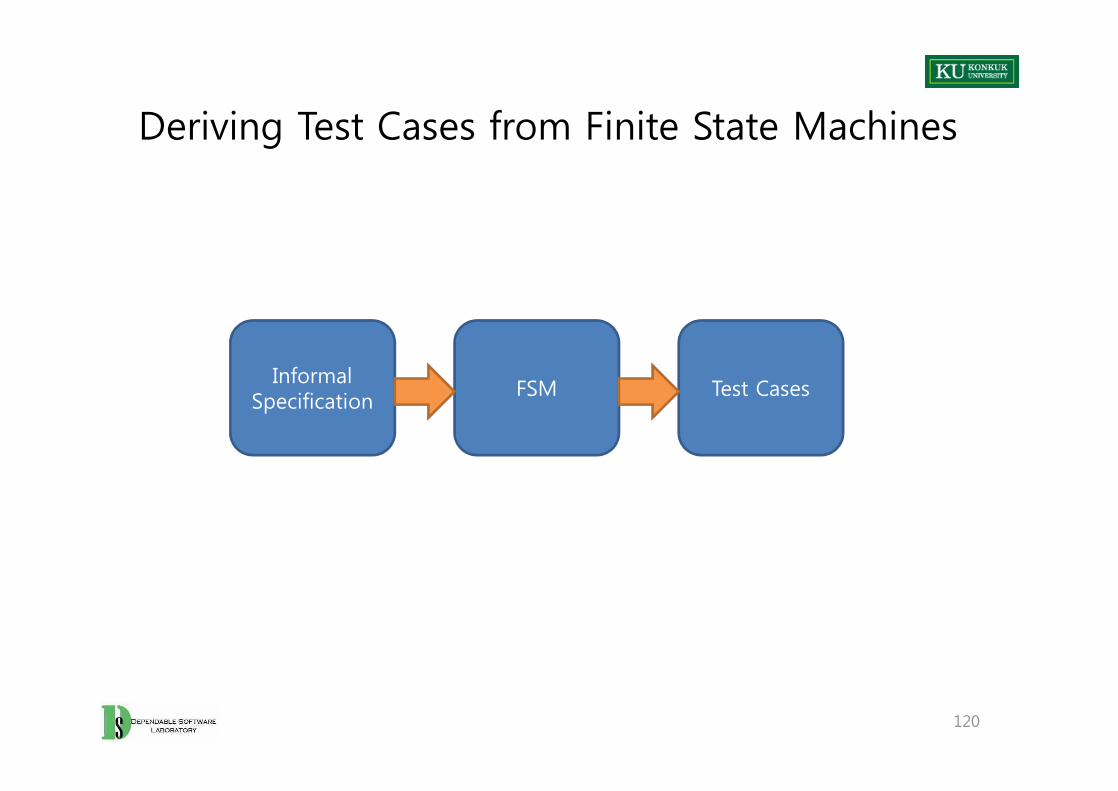
Deriving Test Cases from Finite State Machines
Informal Specification
FSM Test Cases
120
Informal Specification
FSM Test Cases

Informal Specification: Feature “Maintenance” of the Chipmunk Web Site
Maintenance: The Maintenance function records the history of items undergoing maintenance.
If the product is covered by warranty or maintenance contract, maintenance can be requested either by calling the maintenance toll free number, or through the web site, or by bringing the item to a designated maintenance station.If the maintenance is requested by phone or web site and the customer is a US or EU resident, the item is picked up at the customer site, otherwise, the customer shall ship the item with an express courier.If the maintenance contract number provided by the customer is not valid, the item follows the procedure for items not covered by warranty.If the product is not covered by warranty or maintenance contract, maintenance can be requested only by bringing the item to a maintenance station. The maintenance station informs the customer of the estimated costs for repair. Maintenance starts only when the customer accepts the estimate. If the customer does not accept the estimate, the product is returned to the customer.Small problems can be repaired directly at the maintenance station. If the maintenance station cannot solve the problem, the product is sent to the maintenance regional headquarters (if in US or EU) or to the maintenance main headquarters (otherwise).If the maintenance regional headquarters cannot solve the problem, the product is sent to the maintenance main headquarters.Maintenance is suspended if some components are not available.Once repaired, the product is returned to the customer.
121
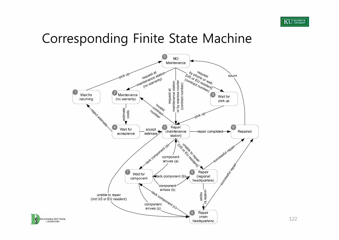
Corresponding Finite State Machine
estim
ate
cost
s
request at
maintenance station
(no warranty)
request by phone or web
[US or EU resident]
(contract number)
pick up
requ
est a
t m
aint
enan
ce s
tatio
nor
by
expr
ess
cour
ier
(con
tract
num
ber)
reject estimate
pick up
invalidcontractnumber
122
estim
atereject estimate
successf
ul repair
unable to repair
(US or EU resident)
succ
essfu
l rep
air
unable to repair
lack co
mponent (a)
lack component (c)
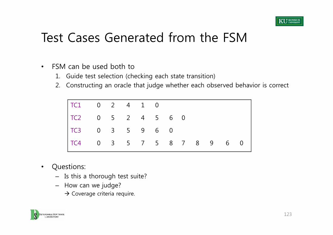
Test Cases Generated from the FSM
• FSM can be used both to1. Guide test selection (checking each state transition)2. Constructing an oracle that judge whether each observed behavior is correct
• Questions:– Is this a thorough test suite? – How can we judge?
à Coverage criteria require.
TC1 0 2 4 1 0
TC2 0 5 2 4 5 6 0
• FSM can be used both to1. Guide test selection (checking each state transition)2. Constructing an oracle that judge whether each observed behavior is correct
• Questions:– Is this a thorough test suite? – How can we judge?
à Coverage criteria require.
123
TC2 0 5 2 4 5 6 0
TC3 0 3 5 9 6 0
TC4 0 3 5 7 5 8 7 8 9 6 0

Transition Coverage Criteria
• State coverage– Every state in the model should be visited by at least one test case.
• Transition coverage– Every transition between states should be traversed by at least one test case. – Most commonly used criterion– A transition can be thought of as a (precondition, postcondition) pair
• State coverage– Every state in the model should be visited by at least one test case.
• Transition coverage– Every transition between states should be traversed by at least one test case. – Most commonly used criterion– A transition can be thought of as a (precondition, postcondition) pair
124
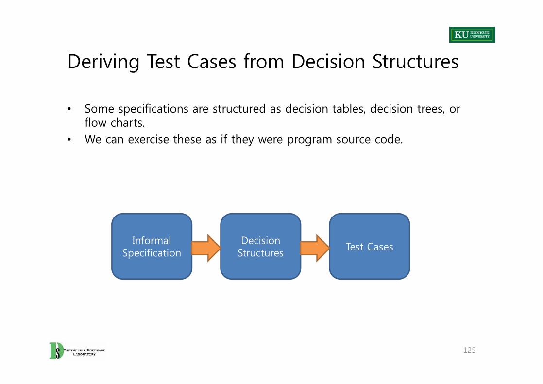
Deriving Test Cases from Decision Structures
• Some specifications are structured as decision tables, decision trees, or flow charts.
• We can exercise these as if they were program source code.
125
Informal Specification
Decision Structures
Test Cases
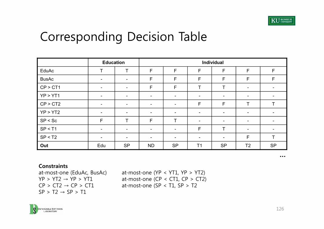
Corresponding Decision Table
Education Individual
EduAc T T F F F F F F
BusAc - - F F F F F F
CP > CT1 - - F F T T - -
YP > YT1 - - - - - - - -
CP > CT2 - - - - F F T T
YP > YT2 - - - - - - - -YP > YT2 - - - - - - - -
SP < Sc F T F T - - - -
SP < T1 - - - - F T - -
SP < T2 - - - - - - F T
Out Edu SP ND SP T1 SP T2 SP
126
…
Constraintsat-most-one (EduAc, BusAc) at-most-one (YP < YT1, YP > YT2) YP > YT2 → YP > YT1 at-most-one (CP < CT1, CP > CT2)CP > CT2 → CP > CT1 at-most-one (SP < T1, SP > T2SP > T2 → SP > T1
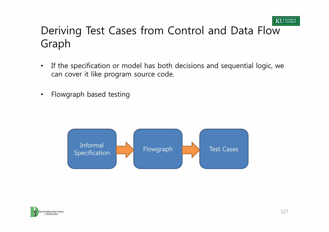
Deriving Test Cases from Control and Data Flow Graph
• If the specification or model has both decisions and sequential logic, we can cover it like program source code.
• Flowgraph based testing
127
Informal Specification
Flowgraph Test Cases
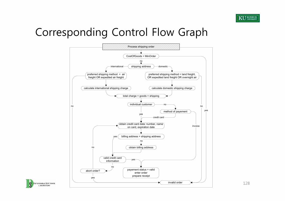
Corresponding Control Flow Graph
preferred shipping method = land freight,OR expedited land freight OR overnight air
Process shipping order
CostOfGoods < MinOrder
shipping address
no
domestic
preferred shipping method = airfreight OR expedited air freight
international
calculate domestic shipping chargecalculate international shipping charge
total charge = goods + shipping
128
yes
individual customer no
yes
obtain credit card data: number, nameon card, expiration date
method of payement
credit card
invoice
billing address = shipping address
obtain billing address
no
yes
valid credit cardinformation
no
yes
payement status = validenter order
prepare receipt
invalid order
nono
abort order?no
yes
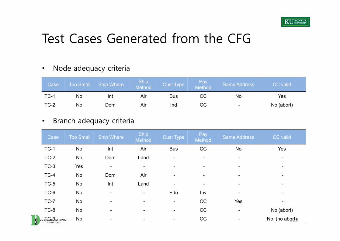
Test Cases Generated from the CFG
• Node adequacy criteria
• Branch adequacy criteria
Case Too Small Ship Where Ship Method Cust Type Pay
Method Same Address CC valid
TC-1 No Int Air Bus CC No Yes
TC-2 No Dom Air Ind CC - No (abort)
• Node adequacy criteria
• Branch adequacy criteria
129
Case Too Small Ship Where Ship Method Cust Type Pay
Method Same Address CC valid
TC-1 No Int Air Bus CC No Yes
TC-2 No Dom Land - - - -
TC-3 Yes - - - - - -
TC-4 No Dom Air - - - -
TC-5 No Int Land - - - -
TC-6 No - - Edu Inv - -
TC-7 No - - - CC Yes -
TC-8 No - - - CC - No (abort)
TC-9 No - - - CC - No (no abort)

Estimating Test Suite Quality
• Supposed that I have a program with bugs.
• Add 100 new bugs– Assume they are exactly like real bugs in every way– I make 100 copies of my program, each with one of my 100 new bugs.
• Run my test suite on the programs with seeded bugs– And the tests revealed 20 of the bugs. – The other 80 program copies do not fail.
• What can I infer about my test suite’s quality?
130
Basic Assumptions
• We want to judge effectiveness of a test suite in finding real faults, – by measuring how well it finds seeded fake faults.
• Valid to the extent that the seeded bugs are representative of real bugs– Not necessarily identical– But, the differences should not affect the selection
• We want to judge effectiveness of a test suite in finding real faults, – by measuring how well it finds seeded fake faults.
• Valid to the extent that the seeded bugs are representative of real bugs– Not necessarily identical– But, the differences should not affect the selection
131
Mutation Testing
• A mutant is a copy of a program with a mutation.
• A mutation is a syntactic change (a seeded bug).– Example: change (i < 0) to (i <= 0)
• Run test suite on all the mutant programs• A mutant is killed, if it fails on at least one test case. (The bug is found.)
• If many mutants are killed, infer that the test suite is also effective at finding real bugs.
132
Assumptions on Mutation Testing
• Competent programmer hypothesis– Programs are nearly correct.
• Real faults are small variations from the correct program.• Therefore, mutants are reasonable models of real buggy programs.
• Coupling effect hypothesis– Tests that find simple faults also find more complex faults.– Even if mutants are not perfect representatives of real faults, a test suite that
kills mutants is good at finding real faults too.
133
Mutant Operators
• Syntactic changes from legal program to illegal program– Specific to each programming language
• Examples: – crp: constant for constant replacement
• E.g. from (x < 5) to (x < 12)• Select from constants found somewhere in program text
– ror: relational operator replacement• E.g. from (x <= 5) to (x < 5)
– vie: variable initialization elimination• E.g. change int x =5; to int x;
134
Fault-based Adequacy Criteria
• Mutation analysis consists of the following steps:1. Select mutation operators2. Generate mutants3. Distinguish mutants
• Live mutants– Mutants not killed by a test suite
• Given a set of mutants SM and a test suite T, the fraction of nonequivalence mutants killed by T measures the adequacy of T with respect to SM.
135

Automating Test Execution
• Designing test cases and test suites is creative.– Demanding intellectual activity– Requiring human judgment
• Executing test cases should be automatic.– Design once, execute many times
• Test automation separates the creative human process from the mechanical process of test execution.
• Designing test cases and test suites is creative.– Demanding intellectual activity– Requiring human judgment
• Executing test cases should be automatic.– Design once, execute many times
• Test automation separates the creative human process from the mechanical process of test execution.
136
From Test Case Specifications to Test Cases
• Test design often yields test case specifications, rather than concrete data.– E.g. “a large positive number”, not 420,023– E.g. “a sorted sequence, length > 2”, not “Alpha, Beta, Chi, Omega”
• Other details for execution may be omitted.
• Test Generation creates concrete, executable test cases from test case specifications.
• A Tool chain for test case generation & execution– A combinatorial test case generation to create test data
• Optional: Constraint-based data generator to “concretize” individual values, e.g., from “positive integer” to 42
– ‘DDSteps’ to convert from spreadsheet data to ‘JUnit’ test cases– ‘JUnit’ to execute concrete test cases
137
Scaffolding
• Code produced to support development activities– Not part of the “product” as seen by the end user– May be temporary (like scaffolding in construction of buildings)
• Scaffolding includes – Test harnesses– Drivers– Stubs
• Code produced to support development activities– Not part of the “product” as seen by the end user– May be temporary (like scaffolding in construction of buildings)
• Scaffolding includes – Test harnesses– Drivers– Stubs
138
Scaffolding
• Test driver– A “main” program for running a test
• May be produced before a “real” main program• Provide more control than the “real” main program
– To drive program under test through test cases
• Test stub– Substitute for called functions/methods/objects
• Test harness– Substitutes for other parts of the deployed environment– E.g. Software simulation of a hardware device
139
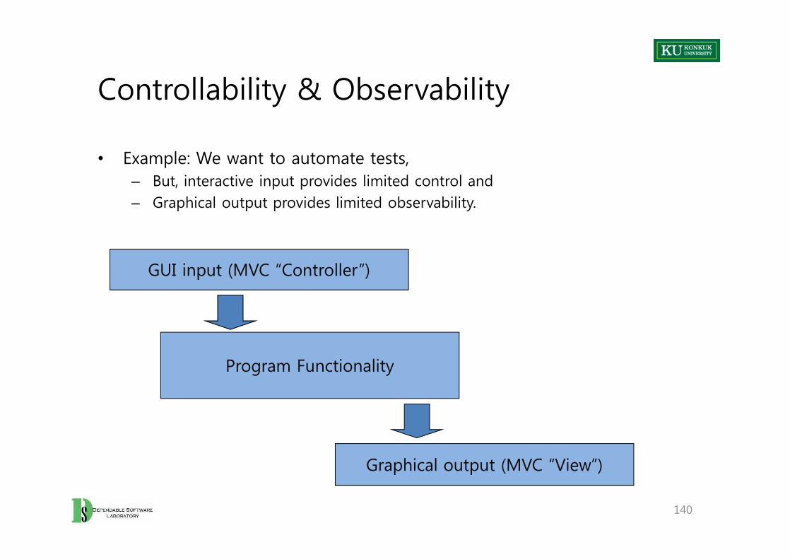
Controllability & Observability
• Example: We want to automate tests, – But, interactive input provides limited control and– Graphical output provides limited observability.
GUI input (MVC “Controller”)
140
GUI input (MVC “Controller”)
Program Functionality
Graphical output (MVC “View”)
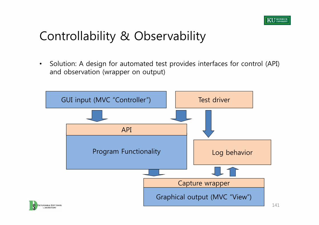
Controllability & Observability
• Solution: A design for automated test provides interfaces for control (API) and observation (wrapper on output)
GUI input (MVC “Controller”) Test driver
141
Program Functionality
Graphical output (MVC “View”)
API
Capture wrapper
Log behavior
Generic vs. Specific Scaffolding
• How general should scaffolding be?– We could build a driver and stubs for each test case.– Or at least factor out some common code of the driver and test management
(e.g. JUnit)– Or further factor out some common support code, to drive a large number of
test cases from data (as in DDSteps)– Or further generate the data automatically from a more abstract model (e.g.
network traffic model)
• It’s a question of costs and re-use, just as for other kinds of software.
142
Test Oracles
• No use running 10,000 test cases automatically, if the results must be checked by hand.
• It’s a problem of ‘range of specific to general’, again– E.g. JUnit: Specific oracle (“assert”) coded by hand in each test case
• Typical approach– Comparison-based oracle with predicted output value– But, not the only approach
143
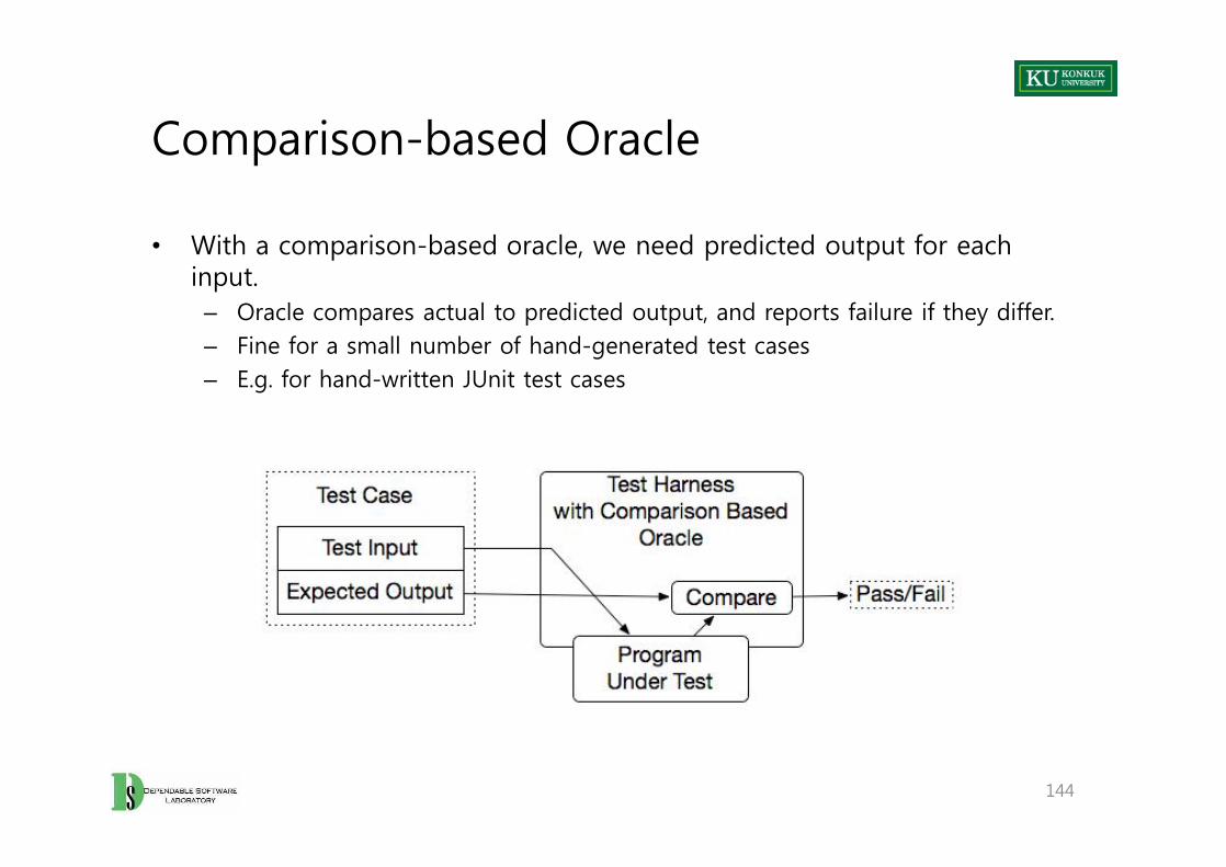
Comparison-based Oracle
• With a comparison-based oracle, we need predicted output for each input.
– Oracle compares actual to predicted output, and reports failure if they differ.– Fine for a small number of hand-generated test cases– E.g. for hand-written JUnit test cases
• With a comparison-based oracle, we need predicted output for each input.
– Oracle compares actual to predicted output, and reports failure if they differ.– Fine for a small number of hand-generated test cases– E.g. for hand-written JUnit test cases
144
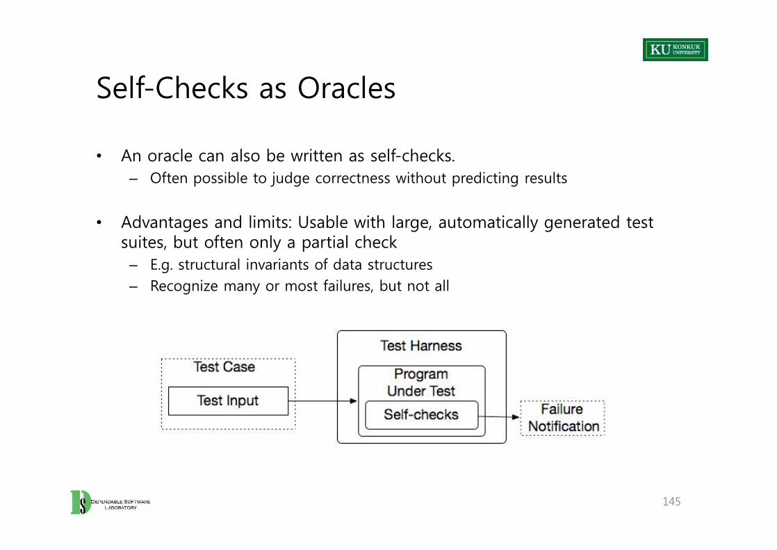
Self-Checks as Oracles
• An oracle can also be written as self-checks.– Often possible to judge correctness without predicting results
• Advantages and limits: Usable with large, automatically generated test suites, but often only a partial check
– E.g. structural invariants of data structures– Recognize many or most failures, but not all
145
Overview
• Automated program analysis techniques complement test and inspection in two ways:
– Can exhaustively check some important properties• Which conventional testing is particularly ill-suited
– Can extract and summarize information for test and inspection design• Replacing or augmenting human efforts
• Automated analysis– Replace human inspection for some class of faults– Support inspection by
• Automating extracting and summarizing information• Navigating through relevant information
146
Static vs. Dynamic Analysis
• Static analysis– Examine program source code
• Examine the complete execution space• But, may lead to false alarms
• Dynamic analysis– Examine program execution traces
• No infeasible path problem• But, cannot examine the execution space exhaustively
• Example:– Concurrency faults– Memory faults
• Static analysis– Examine program source code
• Examine the complete execution space• But, may lead to false alarms
• Dynamic analysis– Examine program execution traces
• No infeasible path problem• But, cannot examine the execution space exhaustively
• Example:– Concurrency faults– Memory faults
147
Extracting Behavior Model from Execution
• Behavior analysis can– Gather information from executing several test cases– And synthesize a model that characterizes those execution,– To the extent that they are the representative of other executions as well.
• Using behavioral models for– Testing : validate tests thoroughness
– Program analysis : understand program behavior
– Regression testing : compare versions or configurations
– Testing of component-based software : compare components in different contexts
– Debugging : Identify anomalous behaviors and understand causes
148