Soil Dynamics and Earthquake Engineering 31 (2011) 1452–1464

Contents lists available at ScienceDirect

Soil Dynamics and Earthquake Engineering

0267-72

doi:10.1

n Corr

E-m

journal homepage: www.elsevier.com/locate/soildyn

An analytical method for strength verification of buried steel pipelines atnormal fault crossings

D.K. Karamitros, G.D. Bouckovalas n, G.P. Kouretzis, V. Gkesouli

Department of Geotechnical Engineering, School of Civil Engineering, National Technical University of Athens, Heroon Polytechniou 9, 15780 Zografou, Greece

a r t i c l e i n f o

Article history:

Received 8 September 2010

Received in revised form

5 May 2011

Accepted 9 May 2011Available online 23 June 2011

61/$ - see front matter & 2011 Elsevier Ltd. A

016/j.soildyn.2011.05.012

esponding author. Tel.: þ30 2107723780; fa

ail address: gbouck@central.ntua.gr (G.D. Bou

a b s t r a c t

The complex problem of strength verification of a buried steel pipeline crossing the trace of a normal

active fault is treated analytically, and a refined methodology for the calculation of the axial and

bending pipeline strains is presented. In essence, the proposed methodology extends the analytical

methodology originally proposed by Karamitros et al. [1] for the simpler case of strike-slip fault

crossings. The modifications introduced to the original methodology are first identified, following a

thorough examination of typical results from advanced 3D nonlinear numerical analyses, and

consequently expressed via an easy to apply solution algorithm. A set of similar numerical analyses,

performed for a wide variety of fault plane inclinations and intersection angles between the pipeline

axis and the fault trace, is used to check the accuracy of the analytical predictions. Fairly good

agreement is testified for pipeline strains up to 1.50–2.00%. It is further shown that, although the

methodology proposed herein applies strictly to the case of right intersection angles, it may be readily

extended to oblique intersections, when properly combined with existing analytical solutions for

strike-slip fault crossings (e.g. [1]).

& 2011 Elsevier Ltd. All rights reserved.

1. Introduction

Buried pipelines are vulnerable to a variety of earthquake-induced hazards, such as permanent ground displacements due tofault rupture or sloping ground failure, or transient grounddisplacements caused by the passage of seismic waves. Althoughless frequent, permanent ground displacements pose a higherthreat to pipelines, as they may impose large axial and bendingstrains and they may lead to rupture, either due to tension or dueto buckling [2]. This is especially true for step-like deformationsresulting from surface faulting, as indicated by a number of casestudies of damage to pipeline systems during strong earthquakes(e.g. [3–6]). Taking further into account the critical role of lifelinesystems to human life support and energy distribution, as well asthe irrecoverable ecological disaster that may result from theleakage of environmentally hazardous materials (e.g. natural gas,fuel or liquid waste), it becomes obvious that the seismic strengthverification of buried steel pipelines at active fault crossings isamong the top design priorities.

A rigorous solution of the problem should involve an advancednumerical analysis which can account consistently for the non-linear stress–strain response of the pipeline steel, the longitudinal

ll rights reserved.

x: þ30 2107723428.

ckovalas).

and transverse soil resistance, typically idealized as a series ofelastic–perfectly-plastic distributed (Winkler) springs, as well assecond order effects induced by large displacements [7]. Suchanalyses are definitely possible with currently available commer-cial computer codes. However, they are rather demanding withregard to computational effort and expertise, so that their use inpractice is justified only for the final design of large diameter,thin-walled pipes and large ground displacements. For morecommon applications, as well as for preliminary pipeline strengthverification purposes, it is desirable to use simplified analyticalmethodologies which will allow reasonably accurate predictionsof pipeline stresses and strains, at a fraction of the computationaleffort required for a rigorous numerical analysis.

Aiming at such a simplified methodology, the mechanismsgoverning the pipeline response at normal fault crossings are firstexplored with the aid of results from 3D elastoplastic finiteelement analyses, for the case of a pipeline with axis perpendi-cular to the fault trace. We consider this experience of firstpriority for two reasons. The first reason is to compare with theassumptions of existing analytical methods (e.g. [1,8–10]) andevaluate their capacity to provide a rational solution to thisproblem. The second, and probably most important reason is toidentify the basic features of the pipeline response and focus uponthem in order to get the required accuracy while avoidingunnecessary complexities which would make an analytical solu-tion impossible or unfriendly to non-specialists.

D.K. Karamitros et al. / Soil Dynamics and Earthquake Engineering 31 (2011) 1452–1464 1453

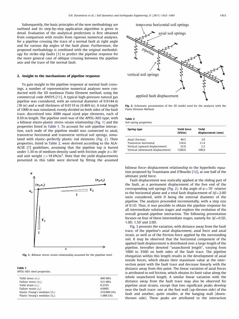
Subsequently, the basic principles of the new methodology areoutlined and its step-by-step application algorithm is given indetail. Evaluation of the analytical predictions is first obtainedfrom comparison with results from rigorous numerical analyses,for a pipeline crossing the trace of a normal fault at right angleand for various dip angles of the fault plane. Furthermore, theproposed methodology is combined with the original methodol-ogy for strike-slip faults [1] to predict the pipeline response forthe more general case of oblique crossing between the pipelineaxis and the trace of the normal fault.

Fig. 2. Schematic presentation of the 3D model used for the analyses with the

Finite Element Method.

Table 2Soil spring properties.

Spring type Yield force(kN/m)

Yielddisplacement (mm)

Axial (friction) 40.5 3.0

Transverse horizontal 318.6 11.4

Vertical (upward displacement) 52.0 2.2

Vertical (downward displacement) 1360.0 100.0

2. Insight to the mechanisms of pipeline response

To gain insight to the pipeline response at normal fault cross-ings, a number of representative numerical analyses were con-ducted with the 3D nonlinear Finite Element method, using thecommercial code ANSYS [11]. A typical high-pressure natural gaspipeline was considered, with an external diameter of 0.9144 m(36 in) and a wall thickness of 0.0119 m (0.469 in). A total lengthof 1000 m was simulated, evenly divided on both sides of the faulttrace, discretized into 2000 equal sized pipe elements, each of0.50 m length. The pipeline steel was of the API5L-X65 type, witha bilinear elasto-plastic stress–strain relationship (Fig. 1) and theproperties listed in Table 1. To account for soil–pipeline interac-tion, each node of the pipeline model was connected to axial,transverse horizontal and transverse vertical soil springs, simu-lated with elastic–perfectly plastic rod elements (Fig. 2). Theirproperties, listed in Table 2, were derived according to the ALA-ACSE [7] guidelines, assuming that the pipeline top is buriedunder 1.30 m of medium-density sand with friction angle f¼361and unit weight g¼18 kN/m3. Note that the yield displacementspresented in this table were derived by fitting the assumed

Fig. 1. Bilinear stress–strain relationship assumed for the pipeline steel.

Table 1API5L-X65 steel properties.

Yield stress (s1) 490 MPa

Failure stress (s2) 531 MPa

Yield strain (e1) 0.233%

Failure strain (e2) 4.000%

Elastic Young’s modulus (E1) 210.000 GPa

Plastic Young’s modulus (E2) 1.088 GPa

bilinear force–displacement relationship to the hyperbolic equa-tion proposed by Trautmann and O’Rourke [12], at one half of theultimate yield force.

Fault displacement was statically applied at the sliding part ofthe fault, as a permanent displacement of the free end of thecorresponding soil-springs (Fig. 2). A dip angle of c¼701 relativeto the horizontal plane and a total fault displacement of Df¼2.0D

were considered, with D being the external diameter of thepipeline. The analysis proceeded incrementally, with a step sizeof 0.1D. Thus, it was possible to obtain the pipeline response forall intermediate solution stages and explore the evolution of theoverall ground–pipeline interaction. The following presentationfocuses on four of these intermediate stages, namely for Df¼0.5D,1.0D, 1.5D and 2.0D.

Fig. 3 presents the variation, with distance away from the faulttrace, of the pipeline’s axial displacement, axial force and axialstrain, as well as of the friction force applied by the surroundingsoil. It may be observed that the horizontal component of theapplied fault displacement is distributed over a large length of thepipeline, hereafter denoted ‘‘unanchored length’’, varying from100D to 350D on both sides of the fault trace. The pipelineelongation within this length results in the development of axialtensile forces, which obtain their maximum value at the inter-section point with the fault trace and decrease linearly with thedistance away from this point. The linear variation of axial forcesis attributed to soil friction, which obtains its limit value along thewhole unanchored length. A similar linear variation with thedistance away from the fault trace may also be observed forpipeline axial strains, except that two significant peaks developnear the fault trace: one at the foot wall (up-thrown side) of thefault and another, quite smaller, at the hanging wall (down-thrown side). These peaks are attributed to the interaction

Fig. 3. Variation of axial displacement, axial force, soil friction forces, as well as

axial strain with the distance away from the fault trace.

D.K. Karamitros et al. / Soil Dynamics and Earthquake Engineering 31 (2011) 1452–14641454

between axial and bending strains, as it will be explained in moredetail in subsequent paragraphs.

The variation of vertical displacements, shear forces, bendingmoments and bending strains, as well as the developing springforces for upward and downward pipeline displacement relativeto the surrounding soil, are presented in Fig. 4. Focusing upon themost intensely deformed, central part of the pipeline, the follow-ing three characteristic points are identified:

Fig. 4. Variation of vertical displacements, shear forces, bending moments,

bending strains and soil resistance forces for upward and downward pipeline

� displacement, with the distance from the fault trace.

Points A and C, on the foot wall and on the hanging wall of thefault, respectively, which are the closest points to the faulttrace where the relative vertical pipeline–ground displace-ment becomes zero.

� Point B which corresponds to the intersection point of the

pipeline axis with the fault trace.

The length of pipeline segment ABC, hereafter denoted ‘‘curvedlength’’, ranges from 35D to 45D, i.e. it is considerably smallerthan the pipeline’s unanchored length. Furthermore, it is notevenly divided on both sides of the fault, with segment BC over

the hanging wall being 3–4 times longer than segment AB overthe foot wall. This is attributed to the different values of soilresistance for upward and downward pipeline displacementrelative to the surrounding soil. More specifically, at the foot wallof the fault (segment AB), soil resistance forces do not reach thecorresponding yield value and increase steadily with applied faultmovements. On the contrary, at the hanging wall of the fault(segment BC), soil resistance forces reach the yield limit at the

D.K. Karamitros et al. / Soil Dynamics and Earthquake Engineering 31 (2011) 1452–1464 1455

early stages of pipeline deformation, practically over the entirelength of this segment. Since upward resistance forces are con-siderably smaller than their downward counter-parts, this seg-ment accommodates most of the vertical component of theapplied fault movement, and is therefore longer than segment AB.

Coming next to shear forces and bending moments developingin the case of small ground displacement (Df¼0.5D), it may beobserved that their distribution along the pipeline axis is typicalof an elastic beam behavior. More specifically, the response ofsegment ABC is, qualitatively at least, similar to that of an elasticbeam, with a triangularly distributed upward load over segmentAB (with peak at B), a uniformly distributed downward load oversegment BC, as well as a downward applied displacement at pointC which is equal to the vertical component of the applied faultdisplacement.

Nevertheless, this simplified model does not accurately repre-sent the actual pipeline response at larger ground displacements,where the axial tension applied on the pipeline exerts significanteffects on bending stiffness and curvature. In this case, plasticstrains accumulate at segment AB, where the maximum bendingmoment occurs. Thus, even though bending strains in this seg-ment significantly increase with increasing fault displacements,the corresponding bending moments decrease. This seeminglycontradictory response is attributed to the following reasons:

�

Figfrom

As the yielding portion of the pipeline cross-section increases,under the combined action of tension and bending, thepipeline’s bending stiffness is reduced [9]. Taking further intoaccount that the pipeline response is displacement and notload controlled, it is realized that this reduction in bendingstiffness is eventually accompanied by a bending momentreduction.

�

Fig. 6. Pipeline deformed shape at normal fault crossings, after Kennedy et al. [9].

The applied axial tension, combined with the pipeline’s step-like deformation mode, has significant geometrical second-order effects on pipeline curvature, resulting also in an overalldecrease of the developing bending moments.

Fig. 5 shows the variation with distance away from the faulttrace of the axial (ea), as well as the minimum (emin) andmaximum (emax) longitudinal pipeline strains, obtained for thecase of large ground displacements (Df¼2.0D). Observe that theaxial strain (ea) does not exhibit a smooth variation, as in the caseof small ground displacements (e.g. Df¼0.5D in Fig. 3), butdevelops a distinct local peak at the point of maximum bendingstrain (eb¼emax�ea¼ea�emin), over the foot wall of the fault. Thisinteraction between axial and bending strains at large grounddisplacements is also a result of the elastoplastic response of thepipeline section. Namely, as maximum strains exceed the yieldlimit of the pipeline steel, axial strains need to increase locally,so that the integral of associated longitudinal stresses over the

. 5. Longitudinal strain distribution over the pipeline cross section (a), and variation o

the fault trace, for a fault displacement of Df¼2.0D (b).

cross-section remains equal to the continuously increasingapplied axial force.

Note that all above observations are in qualitative agreementwith experimental measurements [13] of strain and soil reactionforces developing at HDPE pipelines due to normal faultdisplacement.

3. Evaluation of existing analytical methodologies

The best known methodology for pipeline strength verificationat fault crossings is probably that proposed by Kennedy et al. [9],and consequently adopted by the ASCE [14] guidelines for theseismic design of pipelines, for both strike-slip and normal faults.Kennedy et al. extended the pioneering work of Newmark andHall [8], by taking into account soil–pipeline interaction in thetransverse, as well as in the longitudinal directions. Their meth-odology is based on the assumption that the whole pipelinesection has undergone yielding in the high-curvature zone (ABCin Fig. 4), so that the pipeline’s bending stiffness may be ignored.Nevertheless, it has been previously shown that this assumptionis not true for the displacement range considered herein. In fact,significant bending moments develop along the curved pipelinelength, which persist with increasing fault displacements. It istherefore reasonable to expect that the zero bending stiffnessassumption would result in significant over-estimation of thedeveloping bending strains. Note that Karamitros et al. [1], whileevaluating the performance of the Kennedy et al. [9] methodologyfor strike-slip faults, has shown that the analytically predictedstrains are accurate only for very large fault displacements (i.e.larger than 1.5D), while they may become even one order ofmagnitude larger than the actual ones for the smaller faultdisplacements most commonly considered in practice.

In addition to the above limitation, Kennedy et al. [9] considera plastic hinge at the intersection of the pipeline axis with thefault trace, as shown in Fig. 6, so that relative transverse pipe–soildisplacement only occurs at the hanging wall of the fault. Hence,bending strains developing on the part of the pipeline that lies atthe foot wall of the fault are effectively ignored. This assumption

f minimum, maximum and average (axial) longitudinal strains with distance away

D.K. Karamitros et al. / Soil Dynamics and Earthquake Engineering 31 (2011) 1452–14641456

comes to bold contradiction with the results of the previouslypresented numerical analyses, which clearly indicate that themaximum bending strains occur at the foot wall and not at thehanging wall of the fault.

A more refined analytical methodology was introduced byWang and Yeh [10] for strike-slip fault crossings. They partitionedthe pipeline into four (4) distinct segments: two (2) on both sidesof the fault trace, within the high-curvature zone, and anothertwo (2) on both sides of this zone. The latter are analyzed asbeams-on-elastic-foundation, while the former are assumed todeform as circular arcs, with a radius of curvature calculated fromthe equations of equilibrium and the demand for continuitybetween adjacent segments.

This segmentation allows the pipeline’s bending stiffness to betaken into account, thus overcoming the basic limitation of themethodology of Kennedy et al. [9]. Nevertheless, Wang and Yehoverlook the unfavorable contribution of axial forces on thepipeline’s bending stiffness, thus underestimating bendingstrains. In fact, bending strains are accurately predicted only forvery small fault displacements (i.e. up to 0.3D), where no plasticstrains develop on the pipeline’s cross-section, while for mediumand large fault displacements, they are systematically under-predicted [1].

A number of the afore-mentioned setbacks of the Kennedyet al. [9] and the Wang and Yeh [10] methods have beenefficiently eliminated by Karamitros et al. [1] for the case ofpipeline crossings with strike-slip faults. More specifically:

�

They adopt the pipeline segmentation proposed by Wang andYeh (1977) with one basic difference: the segments thatcorrespond to the high-curvature zone are not treated ascircular arcs, but they are also analyzed as elastic beams, sothat the effect of the varying bending stiffness of the pipelinemay be accurately taken into account. � Material nonlinearity is introduced to the solution algorithm

by assuming a bilinear stress–strain relationship for the pipe-line steel, combined with an iterative equivalent-linear elasticsolution scheme.

� Second-order effects, induced by the combination of large

displacements and axial tension, are indirectly accounted for,through a simplified equation that combines the bendingstrains resulting from the elastic beam analysis, with thebending strains calculated assuming that the pipeline has zerobending stiffness.

� The interaction between axial and bending strains is quanti-

fied by determining the elasto-plastic distribution of strainsand stresses over the pipeline cross-section.

Despite its merits, this methodology is strictly applicable tostrike-slip faults, since it assumes a symmetric pipeline deforma-tion about the intersection point of the pipeline axis with the faulttrace. As it has been shown in the previous section (e.g. Fig. 4),this assumption is grossly inaccurate for normal faults and mayconsiderably underestimate pipeline strains within the highcurvature zone.

The structural model proposed by Karamitros et al. [1] forstrike-slip fault crossings was recently extended to normal faultcrossings by Trifonov and Cherniy [15]. More specifically, theyremoved the symmetry condition about the intersection point,allowing for different types of fault kinematics to be analyzed. Inaddition, the contribution of transverse displacements has beentaken into account for the accurate estimation of the pipeline’saxial elongation. Finally, the two segments in the high-curvaturezone are analyzed as beams under combined bending and tension,so that the axial force is directly included to the governingdifferential equations and the geometrically induced second order

effects are consistently taken into account. The above modifica-tions to the original Karamitros et al. [1] methodology havedefinitely extended its field of application, to strike-slip as wellas to normal fault crossings, but at a significant cost of simplicity.This is because the direct approach adopted by Trifonov andCherniy [15] for simulating second order effects has led to acomplex system of equations which can only be solved withinvolved computationally minimization techniques.

4. Outline of proposed methodology

The proposed methodology aims also to extend the originalmethodology of Karamitros et al. [1] to normal fault crossings,while maintaining the simplicity of the original solution algo-rithm. Hence, an analytical solution is initially established for thespecial case of right (901) intersection angle between the pipelineaxis and the fault trace. It is then shown that the more generalcase of oblique intersection between the pipeline axis and thefault trace can be decomposed into two essentially uncoupledproblems: one of strike-slip fault crossing and the other of normalfault crossing with a 901 intersection angle.

The normal fault considered herein is taken as an inclinedplane, with null thickness of the rupture zone, so that theintersection of the pipeline axis with the fault trace on the groundsurface is reduced to a single point. The fault displacement isdefined in a Cartesian coordinate system, where the X-axis iscollinear with the un-deformed longitudinal axis of the pipelineand the Z-axis is vertical. Subsequently, the fault displacementmay be analyzed into a horizontal and a vertical component, Dx

and Dz, respectively, interrelated through the angle c, formed bythe horizontal axis and the fault plane (Fig. 7).

Since there is no symmetry around the fault–pipeline inter-section point B, the pipeline is partitioned into three segments, asshown in Fig. 7. Partitioning is mainly based on the characteristicpoints A and C, defined in a previous section as the closest pointsto the fault trace where vertical pipeline displacements relative tothe surrounding soil become equal to zero.

Computation of the combined axial and bending pipelinestrains is consequently accomplished in the following six steps.

Step 1: Pipeline segments A0A and CC0 (from �N to A and fromC to þN, respectively) are analyzed as beams-on-elastic founda-tion (Fig. 8), in order to obtain the relation between the shearforce, the bending moment and the rotation of points A and C.

Assuming that pipeline deflections along segments A0A and CC0

remain small for the whole range of applied fault displacements,their response is considered elastic and the differential equationfor the associated elastic lines is written as

E1Iw0000 þkw¼ 0 ð1Þ

Starting with segment CC0 (Fig. 8b) and imposing w¼0 for x¼0and x-N yields:

w¼ C e�lx sinlx ð2aÞ

with

l¼

ffiffiffiffiffiffiffiffiffiffik

4E1I

4

sð2bÞ

In the above equations, x is the distance from point A along thepipeline axis, w is the pipeline’s vertical displacement, E1 is theelastic Young’s modulus of the pipeline steel and k is the verticalsoil spring constant. The value of k is different for upward anddownward pipeline displacement (e.g. [7]). Still, to reduce thenumber of variables, it is possible to use an average value forthe entire segment CC0, regardless of the direction of pipeline

Fig. 8. Structural model for pipeline segments (a) A0A and (b) CC0 .

Fig. 7. Partitioning of the pipeline into three segments.

Fig. 9. Applied convention for positive internal forces (M and V) and displace-

ments (w and j).

D.K. Karamitros et al. / Soil Dynamics and Earthquake Engineering 31 (2011) 1452–1464 1457

displacement, with only minor effect on the overall pipelineresponse.

Differentiation of Eq. (2) yields the following relationsbetween the shear force VC ¼�E1Iw0C , the bending momentMC ¼�E1IwC and the rotation fC ¼w0C at point C. The conventionfor positive internal forces (M and V) and displacements (w and j)used in these relations is shown in Fig. 9. Note that in Fig. 8,internal forces and displacements are shown with their actual andnot the conventional directions, so that the loading and deforma-tion patterns of the pipeline may be more clearly visualized

MC ¼ ð2lE1IÞfC ð3Þ

VC ¼�lMC ð4Þ

Since k is practically the same for both segments, a similarprocedure may be followed for segment A0A (Fig. 8a). More

specifically, the condition of w¼0 is imposed for x¼0 and x-

�N, yielding:

w¼ C elx sinlx ð5Þ

Thus, the following relations may be derived between theshear force VA ¼�E1Iw0A, the bending moment MA ¼�E1IwA andthe rotation fA ¼w0A at point C:

MA ¼�ð2lE1IÞfA ð6Þ

VA ¼ lMA ð7Þ

Step 2: The relations obtained in Step 1 are applied asboundary conditions to central segment ABC in order to computethe associated maximum bending moment.

Pipeline segment ABC (Fig. 10) is analyzed as an elastic beamof total length L and bending stiffness EI. The length L is equal tothe sum of lengths LAB and LBC of pipeline segments AB and BC,lying on the hanging and foot walls of the fault, respectively.Points A and C are supported by rotational springs, whoseconstant is calculated from Eqs. (3) and (6) as Cr ¼ 2lE1I.

Consistent with the results of the numerical analyses inSection 2, a vertical displacement is applied at point C, equal tothe vertical component of the fault displacement Dz. Furthermore,a uniformly distributed load qBC is applied to pipeline segment BC,equal to the limit value of the resistance force, for upwardpipeline displacement relative to the surrounding soil. Asexplained in Section 2, soil reaction forces developing at segmentAB do not exceed the corresponding yield limit, for the entirerange of examined fault displacements. Thus, the actual appliedload along this segment is proportional to the downward dis-placement of the pipeline, being equal to zero at point A and

Fig. 10. Analysis model for pipeline segment ABC.

Fig. 11. Deformation mode of pipeline segment ABC assumed for the estimation of DzB (a) and force diagram for an infinitesimal arc of the curved pipeline length (b).

D.K. Karamitros et al. / Soil Dynamics and Earthquake Engineering 31 (2011) 1452–14641458

obtaining its maximum value at point B. Nevertheless, for thesake of simplicity, a uniformly distributed load qAB will be alsoapplied to segment AB (Fig. 10), equal to one half of unit soilresistance forces developing at point B, i.e.:

qAB ¼kdownDzB

2ð8Þ

where kdown is the stiffness of the respective soil springs. Compu-tation of the vertical displacement DzB follows an approximateprocedure which radically simplifies the resulting equations.Namely, segments AB and BC are simulated as circular arcssubjected to an axial tensile force Fa, as well as to the uniformlydistributed loads qAB and qBC (Fig. 11a). As described in Section 2,the axial force developing at the pipeline obtains its maximumvalue at the intersection point with the fault trace, and decreaseslinearly with the distance from this point. However, this decreaseis due to the applied soil friction and occurs within the ‘‘unan-chored length’’ of the pipeline, which is one order of magnitudelarger than the ‘‘curved length’’. Therefore, in this Step, the axialforce is assumed to remain constant along the lengths AB and BC.Taking the above into account, the respective radii of curvatureRAB and RBC may be readily calculated considering equilibrium of

an infinitesimal arc of these segments (Fig. 11b), as

RAB ¼Fa

qABð9aÞ

RBC ¼Fa

qBCð9bÞ

Note that the above assumption is equivalent with neglectingthe bending stiffness of segment ABC, as if it behaved as a cable.This is similar to what Kennedy et al. [9] have assumed in theirpioneering work, resulting in the prediction of excessive pipelinestrains. Nevertheless, this danger does not exist here as the zerobending stiffness assumption is only considered for the simplifiedcalculation of DzB, while it is reinstated in the remainingcomputations.

For the simplified mode of deformation of Fig. 11, DzB may becomputed in advance, in terms of known problem variables, as

DzB ¼�qBCþ

ffiffiffiffiffiffiffiffiffiffiffiffiffiffiffiffiffiffiffiffiffiffiffiffiffiffiffiffiffiffiffiffiffiffiffiffiffiffiffiffiffiffiqBCðqBCþ2kdownDzÞ

pkdown

ð10Þ

Given the displacement DzB, segment ABC may be analyzedaccording to the elastic-beam theory. More specifically, bendingmoments MA and MC, developing at points A and C, respectively,

D.K. Karamitros et al. / Soil Dynamics and Earthquake Engineering 31 (2011) 1452–1464 1459

may be computed from Eqs. (11a) and (11b). As in Step 1, thismathematical derivation follows the convention for positiveinternal forces and displacements presented in Fig. 9. Therefore,MA is expected to be negative, while MC is expected to be positive,so as to comply with the deformation pattern illustrated in Fig. 10

MA ¼ 4EI

LfAþ2

EI

LfC�6

EI

L2Dz

þqABL2

AB

126�8

LAB

Lþ3

L2AB

L2

� ��

qBCL3BC

12L4�3

LBC

L

� �ð11aÞ

MC ¼�2EI

LfA�4

EI

LfCþ6

EI

L2Dzþ

qABL3AB

12L4�3

LAB

L

� �

�qBCL2

BC

126�8

LBC

Lþ3

L2BC

L2

� �ð11bÞ

Combining the above with Eqs. (3) and (6), yields the followingrelations for the computation of bending moments MA and MC:

MA ¼ð2þðCrL=2EIÞÞMf ¼ 0

A þMf ¼ 0C

4þð6EI=CrLÞþðCrL=2EIÞð12aÞ

MC ¼Mf ¼ 0

A þð2þðCrL=2EIÞÞMf ¼ 0C

4þð6EI=CrLÞþðCrL=2EIÞð12bÞ

where

Mf ¼ 0A ¼�6

EI

L2Dzþ

qABL2AB

126�8

LAB

Lþ3

L2AB

L2

� ��

qBCL3BC

12L4�3

LBC

L

� �ð13aÞ

Mf ¼ 0C ¼ 6

EI

L2Dzþ

qABL3AB

12L4�3

LAB

L

� ��

qBCL2BC

126�8

LBC

Lþ3

L2BC

L2

� �ð13bÞ

Given the bending moments at points A and C, the correspond-ing shear forces may be computed by considering momentequilibrium about points C and A, respectively:

VA ¼1

L�MAþMC�qABLAB L�

LAB

2

� �þ

qBCL2BC

2

� �ð14aÞ

VC ¼1

L�MAþMCþ

qABL2AB

2�qBCLBC L�

LBC

2

� �� �ð14bÞ

Note that, in the above equations, the curved lengths LAB andLBC are not a priori known, and must be estimated iteratively,taking into account the boundary conditions for pipeline segmentABC that were obtained from the analysis of segments A0A and CC0

(Eqs. (4) and (7)). More specifically, initial values of LAB¼5–10D

and LBC¼20–25 D are first assumed, reaction forces at points Aand C are consequently computed using Eqs. (12) and (14), andthe curved lengths LAB and LBC are updated as follows:

L0AB ¼ aqBCLBCþVC�lMA

qABþð1�aÞLAB ð15aÞ

L0BC ¼ aqABLABþVAþlMC

qBCþð1�aÞLAB ð15bÞ

To ensure convergence of the above iterative procedure, thecoefficient a in Eqs. (15a) and (15b) should be chosen between0.20 and 0.50. Note that lengths LAB and LBC calculated from theabove equations are appropriate for the estimation of the max-imum bending moment and strain, as discussed in Step 4, butthey are grossly approximate for the computation of the actualcurved length of the pipeline, which also depends on geometri-cally induced second order effects.

As explained in Section 2, the maximum bending momentMmax develops in segment AB, on the foot wall (up-thrown side)of the fault. Given the reaction forces at points A and C, this

bending moment may be computed as

Mmax ¼MAþVAxmaxþqABx2

max

2ð16aÞ

where

xmax ¼�VA

qABð16bÞ

Step 3: Axial strains developing along the pipeline are inte-grated to compute the pipeline elongation, which is consequentlyidentified as the Dx component of the applied fault displacement,in order to derive the maximum axial force.

The maximum axial force, which develops at the intersectionof the pipeline with the fault trace, may be calculated, based onthe demand for compatibility between the geometrically requiredand the available pipeline elongation. The geometrically requiredelongation DLreq is defined as the elongation imposed to thepipeline due to the fault displacement. In cases where the normalfault plane is inclined (co901), and the pipeline poses adequatebending resistance, the vertical component Dz of the faultdisplacement may be considered to have a negligible effect onpipeline elongation compared to the horizontal component Dx, sothat

DLreq �Dx ð17Þ

On the other hand, the available elongation DLav may bedefined as the integral of axial strains developing along thepipeline’s unanchored length Lanch, on each side of the fault trace,where slippage occurs between the pipeline and the surroundingsoil, i.e.:

DLav ¼ 2

Z Lanch

0eðLÞdL ð18Þ

where L denotes the distance from the fault trace.Taking into account that the soil friction forces which develop

along the pipeline’s unanchored length Lanch are equal to the limitvalue tu, the axial pipeline stresses and the unanchored pipelinelength may be computed as

sðLÞ ¼ sa�tu

AsL ð19Þ

Lanch ¼Fa

tu¼saAs

tuð20Þ

where Fa and sa are the axial force and stress developing at theintersection of the pipeline axis with the fault trace, while As isthe area of the pipeline cross-section.

Assuming further a bilinear stress–strain relationship for thepipeline steel (Fig. 1), Eq. (19) may be used to derive thedistribution of axial strains along the pipeline’s unanchoredlength and consequently calculate the available elongation DLav.Namely, in case that the maximum tensile stress sa is smallerthan the pipeline’s yield stress s1, pipeline strains remain elastic(Fig. 12a) and would be expressed as

eðLÞ ¼ sðLÞE1

ð21Þ

The available elongation may be analytically computed as

DLav ¼ 2

Z Lanch

0

sa�ðtu=AsÞL

E1dL¼

sa2As

E1tuð22Þ

while for DLreq ¼Dx, the maximum tensile stress becomes

sa ¼

ffiffiffiffiffiffiffiffiffiffiffiffiffiffiffiffiE1tuDx

As

sð23Þ

Fig. 12. Linear (sa (point B)os1) (a) and non-linear (sa (point B)4s1) (b) stress and strain variation along the pipeline’s unanchored length.

D.K. Karamitros et al. / Soil Dynamics and Earthquake Engineering 31 (2011) 1452–14641460

If the required elongation is larger than that corresponding tosa¼s1, i.e. when

Dx4DLav,el ¼s2

1As

E1tuð24Þ

plastic strains develop on the pipeline (Fig. 12b) and the corre-sponding available elongation becomes

DLav ¼ 2

Z L1

0e1þ

sðLÞ�s1

E2

� �dLþ

Z Lanch

L1

sðLÞE1

dL

� �ð25aÞ

where

L1 ¼ðsa�s1ÞAs

tuð25bÞ

The maximum developing tensile stress consequently becomes

sa ¼s1ðE1�E2Þþ

ffiffiffiffiffiffiffiffiffiffiffiffiffiffiffiffiffiffiffiffiffiffiffiffiffiffiffiffiffiffiffiffiffiffiffiffiffiffiffiffiffiffiffiffiffiffiffiffiffiffiffiffiffiffiffiffiffiffiffiffiffiffiffiffiffiffiffiffiffis1

2ðE22�E1E2ÞþE1

2E2Dxðtu=AsÞ

qE1

ð26Þ

In either case (Fig. 12a or b), the corresponding axial force isequal to

Fa ¼ saAs ð27Þ

Step 4: Maximum bending strains are computed, taking intoaccount second-order effects induced by the tensile force Fa.

Bending strains developing at the point of the maximumbending moment Mmax may be calculated according to the elasticbeam theory as

eIb ¼

MmaxD

2EIð28Þ

where D is the pipeline diameter. According to Eq. (28), ebI

increases with increasing applied fault displacements. This isnot only due to the anticipated decrease of the equivalent Young’smodulus E when the pipeline steel undergoes yielding, but alsodue to the increase of the maximum bending moment Mmax,calculated according to Eq. (16). However, the numerical analysespresented in Section 2 indicate that the increase of bendingmoments is limited by geometrical second-order effects, arisingfrom the combination of the vertical component of the faultdisplacement and the developing axial tension that was

calculated in Step 3. As a result, Eq. (28) is expected to over-predict bending strains for large applied fault displacements.

In order to take into account the afore-mentioned second-order effects, an upper limit to these strains may be calculated byassuming that the whole pipeline cross-section has undergoneyielding, so that the pipeline’s bending stiffness becomes negli-gible. In this case, the pipeline would essentially behave like acable, and its deformation mode would consist of two circulararcs, as described in Fig. 11. Thus, the resulting bending strainswould become

eIIb ¼

D=2

RAB¼

qABD

2Fað29Þ

According to Eq. (29), bending strains eIIb are inversely propor-

tional to the developing axial force Fa, thus tending to becomeinfinite for small fault displacements.

Summarizing the above, Eq. (28) takes into account thepipeline’s bending stiffness, neglecting second-order effects, andconsequently it is only valid for small fault displacements, whileit overestimates bending strains for larger applied fault displace-ments. On the contrary, Eq. (29) accounts for second-order effects,without taking the pipeline’s bending stiffness into consideration,and consequently it overestimates bending strains for small faultdisplacements while it provides accurate results for large faultdisplacements, when the whole pipeline cross-section has under-gone yielding. Thus, to combine the two, Eq. (30) is introducedwhich asymptotically tends to eI

b when fault displacements tendto zero while it tends to eII

b when fault displacements become verylarge:

1

eb¼

1

eIb

þ1

eIIb

ð30Þ

Step 5: The maximum pipeline strain is computed from stressequilibrium over the pipeline cross section, taking also intoaccount the bilinear elasto-plastic stress–strain relationship forthe pipeline steel.

The numerical results of Section 2 indicate that axial strainsmay increase locally at the point of maximum bending strains, asthe pipeline section starts yielding under the combined action oftension and bending. To quantify this effect, it is first necessary to

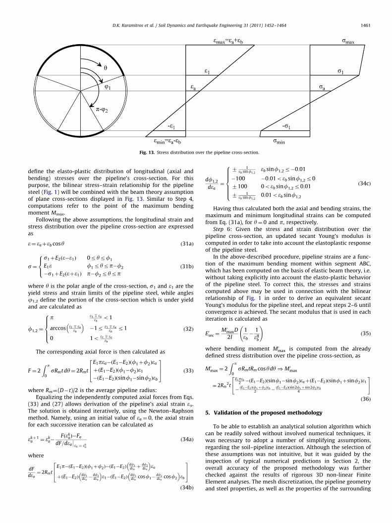
Fig. 13. Stress distribution over the pipeline cross-section.

D.K. Karamitros et al. / Soil Dynamics and Earthquake Engineering 31 (2011) 1452–1464 1461

define the elasto-plastic distribution of longitudinal (axial andbending) stresses over the pipeline’s cross-section. For thispurpose, the bilinear stress–strain relationship for the pipelinesteel (Fig. 1) will be combined with the beam theory assumptionof plane cross-sections displayed in Fig. 13. Similar to Step 4,computations refer to the point of the maximum bendingmoment Mmax.

Following the above assumptions, the longitudinal strain andstress distribution over the pipeline cross-section are expressedas

e¼ eaþeb cosy ð31aÞ

s¼s1þE2ðe�e1Þ 0ryrf1

E1e f1ryrp�f2

�s1þE2ðeþe1Þ p�f2ryrp

8><>: ð31bÞ

where y is the polar angle of the cross-section, s1 and e1 are theyield stress and strain limits of the pipeline steel, while anglesj1,2 define the portion of the cross-section which is under yieldand are calculated as

f1,2 ¼

p e1 8 ea

ebo1

arccos e1 8 ea

eb

� ��1r e1 8 ea

ebr1

0 1o e1 8 ea

eb

8>>><>>>:

ð32Þ

The corresponding axial force is then calculated as

F ¼ 2

Z p

0sRmt dy¼ 2Rmt

E1pea�ðE1�E2Þðf1þf2Þea

þðE1�E2Þðf1�f2Þe1

�ðE1�E2Þðsinf1�sinf2Þeb

264

375 ð33Þ

where Rm¼(D�t)/2 is the average pipeline radius:Equalizing the independently computed axial forces from Eqs.

(33) and (27) allows derivation of the pipeline’s axial strain ea.The solution is obtained iteratively, using the Newton–Raphsonmethod. Namely, using an initial value of ea ¼ 0, the axial strainfor each successive iteration can be calculated as

ekþ1a ¼ ek

a�Fðek

a�Fa

dF=dea9ea ¼ eka

ð34aÞ

where

dF

dea¼ 2Rmt

E1p�ðE1�E2Þðf1þf2Þ�ðE1�E2Þdf1

deaþ

df2

dea

� �ea

þðE1�E2Þdf1

dea�

df2

dea

� �e1�ðE1�E2Þ

df1

deacosf1�

df2

deacosf2

� �eb

264

375ð34bÞ

df1,2

dea¼

7 1eb sinf1,2

eb sinf1,2r�0:01

�100 �0:01oeb sinf1,2r0

7100 0oeb sinf1,2r0:01

7 1eb sinf1,2

0:01oeb sinf1,2

8>>>>><>>>>>:

ð34cÞ

Having thus calculated both the axial and bending strains, themaximum and minimum longitudinal strains can be computedfrom Eq. (31a), for y¼ 0 and p, respectively.

Step 6: Given the stress and strain distribution over thepipeline cross-section, an updated secant Young’s modulus iscomputed in order to take into account the elastoplastic responseof the pipeline steel.

In the above-described procedure, pipeline strains are a func-tion of the maximum bending moment within segment ABC,which has been computed on the basis of elastic beam theory, i.e.without taking explicitly into account the elasto-plastic behaviorof the pipeline steel. To correct this, the stresses and strainscomputed above may be used in connection with the bilinearrelationship of Fig. 1 in order to derive an equivalent secantYoung’s modulus for the pipeline steel, and repeat steps 2–6 untilconvergence is achieved. The secant modulus that is used in eachiteration is calculated as

E0sec ¼M0maxD

2I

1

eb�

1

eIIb

!ð35Þ

where bending moment M0max is computed from the alreadydefined stress distribution over the pipeline cross-section, as

M0max ¼ 2

Z p

0sRmtRm cosydy) M0max

¼ 2Rm2t

E1peb2 �ðE1�E2Þðsinf1�sinf2ÞeaþðE1�E2Þðsinf1þsinf2Þe1

�ðE1�E2Þðf1þf2Þeb

2 �ðE1�E2Þðsin 2f1þ sin 2f2Þeb

4

24

35

ð36Þ

5. Validation of the proposed methodology

To be able to establish an analytical solution algorithm whichcan be readily solved without involved numerical techniques, itwas necessary to adopt a number of simplifying assumptions,regarding the soil–pipeline interaction. Although the selection ofthese assumptions was not intuitive, but it was guided by theinspection of typical numerical predictions in Section 2, theoverall accuracy of the proposed methodology was furtherchecked against the results of rigorous 3D non-linear FiniteElement analyses. The mesh discretization, the pipeline geometryand steel properties, as well as the properties of the surrounding

Fig. 14. Evaluation of analytical predictions with the proposed methodology against results from 3D nonlinear Finite Element analyses.

D.K. Karamitros et al. / Soil Dynamics and Earthquake Engineering 31 (2011) 1452–14641462

soil were kept the same as in Section 2, while three different faultplane angles were considered, c¼ 551, 701 and 851. In each case, atotal fault displacement of Df ¼ 2:0D was applied incrementally,with a step size of 0.1D.

The numerical results are compared to the corresponding analy-tical predictions in Fig. 14. The comparison is made in terms of thevariation, with the normalized fault displacement Df=D, of the peakvalues of axial strain ea, bending strain amplitude eb and total strainsemax¼eaþeb and emin¼ea�eb. A fairly good agreement may betestified, for all components of pipeline strain, for the first twocases of fault plane inclinations (c¼ 551 and 701). For the third caseof a nearly vertical fault plane (c¼ 851), which is rather unusual inpractice, the agreement is equally good for fault displacements up to1.5D (maximum total strain emaxE1%). For larger fault displace-ments, the proposed methodology underestimates both the axialstrain ea and the bending strain amplitude eb. This is mainly a resultof neglecting the effect of the vertical component Dz of the faultdisplacement on the overall pipeline elongation. This simplifyingassumption is realistic for small pipeline strains and inclined faultplanes, but becomes grossly unrealistic as yielding extends over amajor portion of the pipeline cross section, creating essentially a

plastic hinge at the intersection with the fault trace, while the faultplane tends also to become vertical.

6. Application to oblique fault crossings

The methodology proposed in the previous sections has beendeveloped for normal fault crossings, where the pipeline axis isperpendicular to the fault trace. However, it is quite common inpractice to encounter oblique crossings, where the pipelineaxis crosses the fault trace at an angle ba901 (Fig. 15), andthe pipeline displacements develop in the vertical but also in thehorizontal plane through the pipeline axis. In that case, theCartesian coordinate system which was used in the previoussolution scheme has to be redefined. Namely, the X-axis remainscollinear with the un-deformed longitudinal axis of the pipeline,the Z-axis is vertical, while a Y-axis is added in the horizontalplane. The fault displacement Df may be consequently analyzedinto three components, interrelated through angles c and b,defined in Fig. 15:

Dx¼Df coscsinb ð37aÞ

D.K. Karamitros et al. / Soil Dynamics and Earthquake Engineering 31 (2011) 1452–1464 1463

Dy¼Df cosccosb ð37bÞ

Dz¼Df sinc ð37cÞ

Fig. 15. Definition of axes x, y and z and fault displacements Dx, Dy and Dz, for

oblique fault crossings.

Fig. 16. Evaluation of analytical predictions for oblique fault crossi

This general 3D case may be approximately decomposed intotwo simpler 2D cases with known analytical solutions: a strike-slip fault crossing with c¼ 01 and bo901, which can be analyzedwith the methodology of Karamitros et al. [1], and a normal faultcrossing with b¼ 901 and c401, which will be analyzed with themethodology proposed herein.

In order to check the accuracy of this approach, 3D nonlinearFinite Element analyses were performed for three different casesof oblique fault crossing, with b¼c¼ 301, 451 and 601. In the firstcase, the transverse horizontal component of the applied faultdisplacement clearly prevails over the vertical component, whilein the last case the roles are reversed. The numerical algorithm, aswell as the pipeline characteristics and the soil properties, werethe same as the ones presented in Sections 2 and 5 before.

The corresponding numerical results are summarized inFig. 16, with the same format as in Fig. 14. The only differenceis that now the numerical predictions are compared to two sets ofanalytical predictions:

�

ng a

one for strike-slip fault crossing with Dx¼Df coscsinb andDy¼Df cosccosb, obtained with the methodology of Karami-tros et al. [1], and

gainst results from 3D nonlinear Finite Element analyses.

D.K. Karamitros et al. / Soil Dynamics and Earthquake Engineering 31 (2011) 1452–14641464

�

another for normal fault crossing with Dx¼Df coscsinb andDz¼Df sinc, obtained with the methodology presented inthis paper.

It may be observed that, regardless of the prevailing pattern offault displacements (strike-slip or normal fault), the numericalpredictions are in fairly good agreement with the maximum, inabsolute values, of the strains calculated using the strike-slip faultcrossing and the normal fault crossing analytical methodologies.Thus, in the first case, where the transverse horizontal componentof the applied fault displacement is clearly predominant, thenumerical results are fairly well reproduced by the methodologyof Karamitros et al. [1]. On the other hand, in the second and thirdcases, where the vertical component increases relative to thehorizontal, the numerical results gradually approach the analy-tical predictions with the methodology proposed herein.

The reason which justifies the proposed decoupling of perma-nent fault displacements, in this highly nonlinear problem of soil–structure interaction, is that maximum bending moments andlongitudinal strains, resulting from pipeline deformations in ahorizontal and in a vertical plane, are not superimposed, sincethey develop:

�

at different points along the pipeline axis, due to the differentvalues of soil resistance against transverse horizontal andtransverse vertical displacements, and. � at different points on the pipeline cross-section, with 901

central angle difference.

7. Conclusions

The analytical methodology for the stress–strain analysis ofburied steel pipelines crossing active strike-slip faults, proposedby Karamitros et al. [1], is herein extended to the case of normalfaults. Comparison of the analytical predictions with the results ofbenchmark numerical analyses, performed over a wide range offault displacements, fault plane inclinations and intersectionangles, showed fairly good overall agreement, with minor devia-tions which did not generally exceed about 10–20%.

It should be noted that, in its present form, the proposed method-ology applies under the following conditions and limitations:

(a)

The pipeline crosses normal or oblique faults that result inelongation of the pipeline, with tension and bending being theprevailing modes of deformation.

(b)

The pipeline axis is practically straight, while slippage of thepipeline relatively to the surrounding soil is not restrainedalong the pipeline’s unanchored length (e.g. due to bends,anchor plates, etc.).

(c)

The effects of local buckling and section deformation [16] arenot addressed, and consequently the proposed methodologyshould not be extended beyond the strain limits explicitlydefined by design codes (e.g. [7,17]), in order to mitigate suchphenomena in practice.

(d)

Large deviations between analytical and rigorous numericalpredictions were witnessed for nearly vertical fault planes

and relatively large fault displacements (e.g. above 1:25D)where a large part of the pipeline section has undergone yield.

Although the practical significance of the above disclaimerscannot be undervalued, it should be acknowledged that theproposed methodology provides accurate analytical predictionsfor a wide range of pipeline–fault-soil conditions encountered inpractice, while it remains relatively simple and stable and can beeasily programmed for quick application. Still, for the conveni-ence of interested users, the software for spread sheet applicationof the proposed methodology is available at the web site of thesecond author (www.georgebouckovalas.com).

Acknowledgements

The study presented in this paper has been supported by the‘‘EPEAEK II – Pythagoras’’ Grant, co-funded by the European SocialFund and the Hellenic Ministry of Education. This contribution isgratefully acknowledged.

References

[1] Karamitros D, Bouckovalas G, Kouretzis G. Stress analysis of buried steelpipelines at strike-slip fault crossings. Soil Dynamics and Earthquake Engi-neering 2007;27:200–11.

[2] O’Rourke MJ, Liu X. Response of buried pipelines subject to earthquakeeffects. Monograph Series, Multidisciplinary Center for Earthquake Engineer-ing Research (MCEER); 1999.

[3] O’Rourke TD, Lane PA. Liquefaction hazards and their effects on buriedpipelines. Technical report NCEER-89-0007, National Center for EarthquakeEngineering Research, Buffalo, NY, USA, 1989.

[4] O’Rourke TD, Palmer MC. Earthquake performance of gas transmissionpipelines. Earthquake Spectra 1996;20(3):493–527.

[5] EERI. The Izmit (Kocaeli), Turkey earthquake of August 17. EERI SpecialEarthquake Report, 1999.

[6] Uzarski J, Arnold C. Chi-Chi, Taiwan, earthquake of September 21, 1999,reconnaissance report. Earthquake Spectra, The Professional Journal of theEERI 2001;17(Suppl. A).

[7] American Lifelines Alliance. Guidelines for the design of buried steel pipe,July 2001 (with addenda through February 2005), ASCE, 2005.

[8] Newmark NM, Hall WJ. Pipeline design to resist large fault displacement. In:Proceedings of the U.S. national conference on earthquake engineering, AnnArbor, University of Michigan, 1975. p. 416–25.

[9] Kennedy RP, Chow AM, Williamson RA. Fault movement effects on buried oilpipeline. ASCE Transportation Engineering Journal 1977;103(5):617–33.

[10] Wang LRL, Yeh YA. A refined seismic analysis and design of buried pipelinefor fault movement. Earthquake Engineering & Structural Dynamics1985;13(1):75–96.

[11] ANSYS Inc. ANSYS release 12.0 documentation, 2009.[12] Trautmann CH, O’Rourke TD. Behavior of pipe in dry sand under lateral and

uplift loading. Geotechnical Engineering Report 83-6, Cornell University,Ithaca, New York, 1983.

[13] Ha D, Abdoun TH, O’Rourke MJ, Symans MD, O’Rourke TD, Palmer MC, et al.Buried high-density polyethylene pipelines subjected to normal and strike-slip faulting—a centrifuge investigation. Canadian Geotechnical Journal2008;45(12):1733–42.

[14] ASCE Technical Council on Lifeline Earthquake Engineering. Differentialground movement effects on buried pipelines. Guidelines for the SeismicDesign of Oil and Gas Pipeline Systems; 1984.

[15] Trifonov OV, Cherniy VP. A semi-analytical approach to a nonlinear stress–strain analysis of buried steel pipelines crossing active faults. Soil Dynamicsand Earthquake Engineering 2010;30(11):1298–308.

[16] Takada S, Hassani N, Fukuda K. A new proposal for simplified design of buriedsteel pipes crossing active faults. Earthquake Engineering and StructuralDynamics 2001;30(8):1243–57.

[17] Comite Europeen de Normalisation. Eurocode 8: Design of structures forearthquake resistance, Part 4: Silos, tanks and pipelines, CEN EN 1998-4,Brussels, Belgium, 2006.