soil moisture sensitivity to nrl-blend high-resolution precipitation products: analysis of...

32 IEEE JOURNAL OF SELECTED TOPICS IN APPLIED EARTH OBSERVATIONS AND REMOTE SENSING, VOL. 3, NO. 1, MARCH 2010

Soil Moisture Sensitivity to NRL-BlendHigh-Resolution Precipitation Products: Analysisof Simulations With Two Land Surface Models

F. Joseph Turk, Member, IEEE, Georgy V. Mostovoy, and Valentine G. Anantharaj

Abstract—We examine the Naval Research Laboratory (NRL)blended satellite (NRL-Blend) High-Resolution PrecipitationProduct (HRPP) as a proxy for a Global Precipitation Mission(GPM)-era HRPP by using the NRL-Blend for precipitationforcing in land surface models (LSM). We use the existing (late2008) constellation of low Earth orbiting (LEO) microwave-basedsatellite platforms as a baseline to examine the impact of omittingseveral satellite and sensor types from future GPM-era HRPPs. Aresponse of 1-m soil water content (SWC) to different precipitationforcing represented by six NRL-Blend satellite/sensor omissionscenarios was investigated using simulations over the centralUnited States with the Noah and Mosaic land surface models(LSM). The LSMs were integrated over a domain encompassingthe Arkansas-Red River basin, using the North American LandData Assimilation System (NLDAS) atmospheric forcing (exceptfor precipitation). Both spatial and temporal statistical propertiesof the SWC response were examined. Both LSMs predicted arather consistent geographical response of the 1-m SWC to dif-ferent precipitation inputs, having positive/negative SWC monthlymean anomalies in western/eastern parts of the domain. Thebiggest impact was due to the omission of either the crosstrackmicrowave sounders, or the morning local time crossing satellites.On the other hand, omission of afternoon local time crossing satel-lites in the NRL-Blend resulted in the smallest impact upon thesoil moisture simulated both with the Noah and Mosaic models.Although the relative magnitude of these SWC changes is small,these results suggest the importance of the crosstrack microwavesounders for future GPM constellations.

Index Terms—Global Precipitation Mission (GPM), Hydrology,microwave radiometry, modeling, precipitation, remote sensing,satellites.

I. HIGH-RESOLUTION PRECIPITATION PRODUCTS (HRPP)

H IGH-resolution precipitation products (HRPP) com-bine a multitude of spaceborne remotely-estimated

and ground-based datasets in order to generate a fine spatial

Manuscript received March 18, 2009; revised September 07, 2009. First pub-lished November 10, 2009; current version published February 24, 2010. Thiswork was supported by the NASA Applied Sciences Program under contractNNS06AA98B. F. J. Turk’s contribution to this work was performed at the JetPropulsion Laboratory, California Institute of Technology, under contract withthe National Aeronautics and Space Administration.

F. J. Turk is with the Jet Propulsion Laboratory, Pasadena, CA 91109-8099USA (e-mail: [email protected]).

G. V. Mostovoy and V. Anantharaj are with the GeoSystems ResearchInstitute, Mississippi State University, Starkville, MS 39762 USA (e-mail:[email protected]; [email protected]).

Color versions of one or more of the figures in this paper are available onlineat http://ieeexplore.ieee.org.

Digital Object Identifier 10.1109/JSTARS.2009.2034024

and/or temporal-resolution precipitation product. These HRPPsare relevant to a variety of applications relating to Earth’shydrological cycle. Passive microwave sensors onboard lowEarth orbiting (LEO) and geostationary Earth orbiting (GEO)environmental satellite systems provide the basic buildingblocks of HRPPs, augmented in some cases by surface radarand raingauge information and analyses from numericalweather prediction (NWP) models. Examples of commonlyused HRPPs are the Tropical Rainfall Measuring Mission(TRMM) Multisatellite Precipitation Analysis (TMPA) [1], thePrecipitation Estimation from Remotely Sensed Informationusing Artificial Neural Networks (PERSIANN) datasets [2],the Climate Prediction Center morphing technique (CMORPH)[3], and the NRL-Blend [4], among others. Typically, theseHRPPs combine multiple satellite datasets (and some add inadditional raingauge and other nonsatellite data) and produceestimates of three-hourly accumulated precipitation between

60 degrees latitude, updated every three hours, at a griddedspatial resolution of 0.25-degrees. From these three-hourlyaccumulations, longer time scale accumulations can be gener-ated. Some of these HRPPs are designed to be operated strictlyin near realtime (e.g, NRL-Blend), while others create nearrealtime as well as a higher quality, postprocessed nonrealtimedatasets.

II. NRL-BLEND HRPP TECHNIQUE

In this section, we outline the design and implementation ofthe NRL blended satellite precipitation technique (referred toas NRL-Blend), which is based upon a real time, underlyingcollection of time and space-matching pixels from all opera-tional geostationary (GEO) visible/infrared (VIS/IR) imagersand passive microwave (PMW) imagers onboard low Earthorbiting (LEO) satellites. It operates in an autonomous, oper-ational mode with a steadily arriving stream of near real-timedata from the operational GEO and LEO satellites [4]. Asof January 2009, the current operational GEO satellites areGOES-11, GOES-12, Meteosat-7, Meteosat-9 (MSG-2), andGMS-6 (MTSAT-1R). The current LEO constellation usedin tabulated in Table I, along with the associated rainfall ratealgorithm used for each sensor. The local time of ascendingnode (LTAN) of most of these satellites (Aqua is maintainedclosely at 1330) is allowed to drift, so the times are provided forthe beginning of 2009. All of these satellites orbit sun-synchro-nously with the exception of TRMM (TRMM’s local observingtime repeats approximately every 28 days at the equator).Note that NOAA-15/17, Metop, all DMSP, and Coriolis are in

1939-1404/$26.00 © 2010 IEEE

TURK et al.: SOIL MOISTURE SENSITIVITY TO NRL-BLEND HIGH-RESOLUTION PRECIPITATION PRODUCTS 33

TABLE ILOW EARTH ORBITING (LEO) ENVIRONMENTAL SATELLITES AND THE ASSOCIATED PASSIVE AND ACTIVE MICROWAVE SENSORS

USED IN THE NRL-BLEND, AS OF EARLY 2009

orbit patterns which crossover in mostly morning (AM) andevening (within a few hours of the solar terminator), whereasNOAA-16/18 and Aqua are in orbits which crossover in earlyafternoon (PM) and early morning (NOAA-16 is an operationalbackup which has drifted from its initial PM 1400 LTAN tonear 1720 as of 2009). AMSU-B and MHS are crosstrackscanning sounders which can be used also for precipitation es-timation, PR is an across-track scanning radar, whereas SSMI,SSMIS, WindSat and AMSR-E all scan conically. Althoughthe NRL-Blend is operated with all of these LEO datasets tominimize overall revisit time, as an option any of these LEOdatasets can be omitted such as to study, for example, how theloss of a particular satellite in a particular orbit will affect theoverall performance of the NRL-Blend. This option will proveuseful when the land surface hydrology modeling is examinedin Section IV.

The operation of the NRL-Blend is essentially described bythree procedures [4]: a) background collocation of time/spaceintersecting pixels from all operational geostationary (GEO)visible/infrared (VIS/IR) imagers and passive microwave(PMW) imagers, b) use of these collocated data for adjustmentof VIS/IR data into instantaneous rainrates, and c) updates of3, 6, 12, and 24-hour interval accumulations updates at eachthree-hourly synoptic time (00, 03, 21 UTC). For the TRMMPR, the near surface rain data in the TRMM-2A25 dataset isused, which is the highest resolution rainfall product available(4 km) from all of the algorithms listed in Table I. Althoughthe computations are done on a 0.1 latitude-longitude gridbetween 60 degrees latitude, the archived products are aver-aged to a global 0.25 grid (480 lines 1440 samples). TheNRL-Blend was operated intermittently beginning in 2002, butofficial data collection of the global precipitation accumulationproducts began in January 2004.

III. GROUND VALIDATION

Much of the verification of the NRL-Blend and other HRPPshas taken place with ground-based raingauge networks as

part of the verification activities of the International Precip-itation Working Group (IPWG). Turk et al. [5] validated theNRL-Blend at various space and time scales using a denseraingauge network. Ebert et al. [6] presented a summary of theover-land validation of 12 HRPPs and four numerical weatherprediction (NWP) models (including the Navy OperationalGlobal Atmospheric Prediction System, NOGAPS) done ona daily time scale and at a 25-km spatial resolution, using theAustralian Bureau of Meteorology daily raingauge analysis[7]. The results demonstrated that the NRL-Blend (and otherHRPPs) precipitation occurrence and amount were more accu-rate than NOGAPS (and other NWP models) during summermonths and lower latitudes. Conversely, NOGAPS (and otherNWP models) exhibited superior performance compared tothe NRL-Blend (and other HRPPs) during winter months andmid-latitudes. Since models transport the moisture with thedynamical state of the atmosphere, the models generally doa better job of following the movement of precipitation asso-ciated with mid-latitude frontal systems. Sapiano and Arkin[8] analyzed the performance of several three-hourly HRPPaccumulations over the central United States, and with anocean buoy network in the tropical Pacific Ocean. The resultsshowed that the NRL-Blend did resolve the diurnal cycle ofprecipitation, but with a high bias over land. The Programfor the Evaluation of High-Resolution Precipitation Products(PEHRPP), sponsored by the IPWG, provides a forum forfuture validation activities [9].

A. Satellite/Sensor Omission Experiments

In this section, a unique series of satellite-denial experimentsare presented which are aimed towards understanding how theperformance of an adjustment-type HRPP (the NRL-Blend) isaffected by the types of satellite sensors employed in the un-derlying LEO satellite constellation. The Global PrecipitationMission (GPM) is an upcoming joint Earth observation missionbetween the National Aeronautics and Space Agency (NASA)and the Japanese Aerospace Exploration Agency (JAXA) [13],


[14]. It builds upon the heritage of the Tropical Rainfall Mea-suring Mission (TRMM) with an advanced core spacecraft aug-mented by a constellation satellite and other international satel-lite systems with precipitation-sensing capabilities. However,with changes to satellite missions and sensor capabilities, it isunlikely that the satellites forming the GPM constellation con-figuration will be known until close to the launch of the corespacecraft, and will change during the lifetime of the GPM.Therefore, it is instructive to study how the retention or lossof a particular satellite platform and/or sensor type will affectthe performance of the GPM precipitation products and otherapplications that utilize GPM products. Therefore, we examinehow the performance of the NRL-Blend is impacted when oneor more satellite systems are omitted, using the existing (late2008) PMW satellite constellation to examine the impact of sev-eral proxy GPM satellite constellation configurations.

In order to examine the these impacts, the NRL-Blend wasconfigured for ten parallel runs, each run employing differentcombinations of satellites and sensor types, beginning in June2007. Each of these runs employed a different set of satellitesrelative to the “All Satellites” configuration. The “All Satellites”baseline run, as the name suggests, utilized all 12 available lowEarth-orbiting satellites for a total of 13 sensors, described inTable I (NOAA-19 had not yet been implemented). The otherparallel runs of the NRL-Blend were configured to specificallystudy the impact of omitting either the local morning (AM) orafternoon (PM) crossing satellites, and the impact of omittingthe crosstrack microwave sounding sensors. The reasoning be-hind the latter is that owing to changes to satellite programs andsensors could lead to the omission of the preferred conically-scanning microwave imagers, leading to a increased role forthe crosstrack microwave sounders (designed mainly for tem-perature and humidity profiling and not precipitation sensing)than originally envisioned in GPM. Microwave sounding sen-sors such as AMSU, MHS, and the future Advanced TechnologyMicrowave Sounder (ATMS) are typically placed in AM or PMsun-synchronous orbits to satisfy observational requirements forNWP data assimilation applications. Several recent studies andalgorithms have demonstrated that the AMSU channel suite,with its suite of sounding and window channels, is capable ofimproved detection of precipitation at high latitudes [11]. It is,therefore, instructive to determine how the performance of theNRL-Blend (the concept could be extended to any HRPP) is im-pacted by the loss of satellite systems with microwave soundingsensors.

B. Ground Validation

We use the optimal interpolation (OI) daily 0.5 griddedgauge analysis provided by the National Oceanic and Atmo-spheric Administration (NOAA) Climate Prediction Center(CPC) [10] for ground validation. The focus areas are overthe continental United States during two three-month periods,June–August 2007 (JJA) and December 2007–February 2008(DJF). For ease of interpretation with [6], the panels in Fig. 1use the identical box-and-whiskers type presentation, using thesame 1 mm day threshold for rain detection. The panels fromtop to bottom are bias, equitable threat score (ETS), probabilityof detection (POD) and false alarm rate (FAR). The left figure

only considers data west of 100 W longitude (generally higherelevation terrain, colder surface backgrounds), and the rightfigure is for data east of 100 W longitude. The colors refer todifferent runs of the NRL-Blend each with a different set ofsatellites. For example, “No AM XT” refers to the NRL-Blendprecipitation estimates when all morning (time of ascendingnode near 1800 local) satellites with crosstrack sounderswere omitted from the “All Satellites” configuration of theNRL-Blend. “No PM XT” refers to the NRL-Blend precipita-tion estimates when all afternoon (time of ascending node near1330 local) satellites with crosstrack sounders were omitted.Only one NWP model (NOGAPS) is shown (gray color). Byintercomparing the bias, ETS, POD and FAR side-by-side, onecan notice where one satellite combination performed better orworse than another and relative to the NOGAPS model, duringsummer and winter seasons, and at lower and higher elevations.

In general, there is overall performance degradation for allruns of the NRL-Blend over the western United States (U.S.)compared to the eastern US. This is consistent with studies thathave shown the poor performance of PMW scattering-basedtechniques when used over high elevation and complex terrain[12]. At first inspection, there is not much difference amongstthe various satellite omission runs for the NRL-Blend, but closerinspection (green box) illustrates largest performance impact isthe omission of the morning overpass crosstrack sounders (“NoAM XT” and “No AM” configurations). On the one hand, thisis encouraging, since many potential constellation members forGPM are operational platforms with NWP as a primary mission(e.g., MetOp, NPP, and NPOESS), and the MHS and ATMS mi-crowave sounders on these satellites are key instruments. Onthe other hand, developing merged PMW precipitation datasetsfrom mixtures of cross- and conically scanning sensors is a chal-lenging task, since the variable fields of view (FOV) and inci-dence angles needs to be considered. In the next section, we ex-amine if land surface models exhibit similar results when theyare forced with precipitation from these NRL-Blend datasets.

IV. SENSITIVITY OF LAND SURFACE STATES

The science objectives of GPM also include hydrometeoro-logical prediction capabilities for flood hazard and fresh waterresource modeling and prediction, as well as quantifying the im-provements in the estimation and partitioning of land surfaceparameters of runoff/infiltration/storage and latent/sensible heatfluxes. Hence, it is helpful to quantify and understand the sen-sitivities of some of the commonly used land surface models(LSM) to uncertainties in the satellite-derived precipitation es-timates. We use the suite of NRL-Blend data from the satelliteomission experiments as GPM proxy data to force the LSMs,and then estimate the sensitivities of the different models to dif-ferences in the precipitation forcing data.

A. Configuration of Land Surface Models

Impact and validation efforts also include the use of LSMsand other types of hydrological observations (other than rain-gauge as was done above) to examine the impact of these GPMproxy data upon streamflow, discharge, soil moisture and other


runoff measurements. By employing the Noah [15] and the Mo-saic [16] LSMs, incorporated with the NASA Land Informa-tion System (LIS) [17] to simulate land surface and hydrolog-ical states, the performance impact of different GPM constel-lations can be examined. A similar methodology was used byGottschalk et al. [18] to study the impact of different precip-itation products on soil states simulated by the Mosaic LSMover the continental United States. Precipitation is consideredas an important factor in controlling spatial and temporal pat-terns of the soil moisture, especially in arid and semi-arid re-gions [19]. The analysis domain selected for this study coversthe south-central United States where there is a large numberof well-instrumented watersheds in the Arkansas and Red Riverbasins [20]. In Fig. 2(a), we show the geographical distributionof accumulated precipitation from the NRL-Blend “All Satel-lites” configuration during 1 April to 31 August 2008, and inFig. 2(b) during August 2008 only.

The Noah LSM (version 2.7.1) was used for retrospective soilmoisture simulations with four standard soil layers having thick-ness (from top to bottom) of 10, 30, 60, and 100 cm. Also, theMosaic model had a standard configuration with three soil layershaving the following thickness: 2 cm, 158 cm, and 200 cm. Bothmodels were configured at a latitude-longitude gridover this longitude latitude experimental domain. Inboth LSMs, soil moisture is predicted from a numerical solu-tion of the diffusion-type equation [21]. Water movement in thesoil depends on hydraulic properties (saturated conductivity andmatrix potential, porosity and others) of the soil substrate.

Soil temperature prediction is based on the heat diffusionequation, which is numerically solved for four soil layers in theNoah model, but a simpler approach based on the force-restoremethod is adopted in the Mosaic model to predict the soil tem-perature only in two layers (surface and deep) [22]. Note thatthe surface temperature , which is equal to the canopy tem-perature, is estimated from the prognostic energy balance equa-tion in the Mosaic model. Conversely in the Noah model, isevaluated diagnostically from an equation of the surface energybudget, linearized in . Therefore, the Mosaic LSM impliessome heat storage (the term is nonzero) within the thinsurface layer having a finite thickness, which includes both thesoil substrate and the canopy air. Due this reason in part, the Mo-saic model has a relatively thinner top soil layer of only 2 cm.But in the Noah model the term is assumed to be zero,and this fact suggests a zero thickness of the surface layer and,therefore, no heat storage within it. Additional details regardingthe differences in the surface layer description have been pre-sented by Smirnova et al. [23].

Surface static fields (vegetation fraction, leaf and stem areaindices, soil porosity and texture, sand/clay/silt fraction, eleva-tion, slope, and others), which are necessary for the land statesimulations with the LSMs, are bilinearly interpolated or aggre-gated from their native grids (most of these fields are availableat 0.01 grid spacing) to the latitude-longitude gridusing routines available from the NASA LIS. In order to pro-duce realistic soil moisture fields, both LSMs were integratedfor a 2.5 year period (1 January 2005 to 1 June 2007) usingthe North American Land Data Assimilation System (NLDAS)forcing fields including precipitation [24]. Initially, a constant

30% volumetric moisture content was assigned at all model gridpoints. The 2.5 year spin-up time was used to produce realisticspatial variations of soil moisture fields within the integrationdomain. Then, the Noah and Mosaic LSMs were additionally in-tegrated for 14 months (until 31 August 2008) using six differentNRL-Blend precipitation products and the NLDAS atmosphericfields (except for precipitation). Hourly soil moisture values out-putted from both LSMs were averaged to produce daily meanvalues, and these daily values of soil moisture were used as abasis for the analysis described in the next section.

B. Sensitivity Analysis of Monthly Averages

A top 1-m soil water content (SWC) was used as an inte-gral soil moisture measure to compare simulation capabilitiesbetween Noah and Mosaic LSMs in reproducing a response ofthe soil moisture to variations in precipitation. Usually, the totalSWC within a column is measured in length units (mm or cm)and can be considered as the amount of water stored in the con-trol volume represented, in our case, by the 1-m soil columnhaving the unit cross-section area. Due to this definition, theSWC is also known as the water storage [25], [26]. Either thewater storage (or the column SWC) and its temporal change/range at monthly and seasonal scales are broadly adopted forthe LSM intercomparison. Previous studies have shown that thelocal maximum water holding capacity of the soil substrate (de-fined as the SWC difference between saturation and wiltingpoints, which depend on the soil texture) has a little impactupon the observed and simulated water storage range [25], [26].Rather, they have suggested that the monthly/seasonal waterstorage changes are controlled by the description of the model’sevaporation and runoff.

In order to better understand the seasonal variations of theimpact of the various NRL-Blend precipitation products on thesimulated SWC, we focused on a monthly analysis of SWCdifference relative to the “All Satellites” configuration duringMarch–August 2008. Before performing an intercomparison be-tween SWC fields produced by the six NRL-Blend precipita-tion products, monthly mean SWC fields simulated using the“All Satellites” precipitation product (“All Satellites” clima-tology) will be described. Fig. 3(a) illustrates the geographicaldistribution of top 1-m SWC simulated with Noah and MosaicLSMs, and averaged for August 2008. Although there is a gen-eral agreement in geographical patterns of 1-m SWC simulatedby the two LSMs (the corresponding correlation between theNoah and Mosaic SWC fields is as high as 0.67), the SWCvalues produced by the Mosaic model are substantially underes-timated in comparison to those simulated by the Noah LSM. Themean top 1-m SWC difference (bias) between Noah and Mosaic(Noah minus Mosaic value) simulations is 8.3 cm for August2008. This rather large SWC bias demonstrated by the Mosaicmodel might be attributed to more efficient surface evaporationand drainage through the lower boundary of the soil column,accounting for the slope of the model grid cell, as comparedto that in the Noah LSM. Comparisons between observed andsimulated top 2-m SWC performed over the state of Illinois alsoindicated a low SWC bias predicted by the Mosaic model, es-pecially for SWC 50 cm, and almost zero bias for the NoahLSM [26]. Fig. 3(b) shows the April–August SWC (top 1-m


Fig. 1. (a) Seasonal performance of the NRL-Blend HRPP over the continental United States during two three-month periods, June–August 2007 (JJA) andDecember 2007–Februa4ry 2008 (DJF), using different satellite combinations and a threshold of 1 mm day . From the top, bias, equitable threat score (ETS),probability of detection (POD), and false alarm rate (FAR) from ten versions of the NRL-Blend and the NOGAPS NWP model. Each version is denoted by a color,which refers to a different set of satellites that was omitted from the NRL-Blend, relative to the “All Satellites” baseline product. “No XT” refers to no crosstracksounders, “No AM XT” refers to no morning nodal crossing crosstrack sounders, “No TMI+PR+Aqua” refers to no TRMM TMI and PR and no AMSR-E fromAqua. “NOGAPS” is the 24-hour forecast from the Navy global NWP model. (a) For areas west of 100 W longitude. (b) Same as (a), but for areas east of 100 Wlongitude.

Fig. 2. (a) Geographical distribution of accumulated precipitation (cm) from the NRL-Blend “All Satellites” configuration during 1 April to 31 August 2008.(b) Same as above, but during August 2008 only.

water storage) change simulated by the Noah and Mosaic LSMs.Despite differences in the model physics, both LSMs producehighly-correlated spatial patterns of the water storage change.These patterns include areas of drying (positive values of SWCchange) in the NW and SE parts of the domain, and a distinct

zone of moistening (negative values) stretching from the SW tothe NE corner of the domain.

C. Water Storage Sensitivity

A simple definition of the soil water budget will be used toestimate the soil moisture sensitivity to precipitation variations.


Fig. 3. (a) Geographical distribution of the top 1-m soil water content (averaged for August 2008) and (b) its change from 1 April to 31 August 2008, simulatedwith the Noah (upper frame) and Mosaic (lower frame) land surface models, using the “All Satellites” NRL-Blend precipitation product. Positive values shownby brown color in right frames stand for soil drying and negative (green/blue) for soil moistening. The thick line outlines the boundary of the Arkansas-Red Riverbasin.

At every grid point of LSMs, SWC temporal changes are relatedto precipitation , surface runoff , and evaporation ratesthrough the water budget equation as follows:

(1)

where is the top 1-m soil water content SWC. Note that bothand rates are nonlinear functions of . Usingto denote the soil water content (storage) change during the

time period and symbol to specify variationsin , , , and variables, (1) can be numerically integratedand rewritten as

(2)

where the symbol stands for infiltration rate which is equal to, and is the total number of days within a given

time period. Generally, represents variation or any kind ofuncertainty (e.g, precipitation measurements errors, deviationsfrom ensemble mean, etc.) and in the present study standsfor the precipitation difference between a particular NRL-blendsatellite omission product and the “All Satellites” configuration.Both differential (1) and integral (2) forms of the water budgetequation were amply used in analytical and empirical studiesof precipitation variations on the structure of soil moisture timeseries [27]–[29].

Equation (2) states that changes (during a given pe-riod) are due to accumulated changes in and . Denotingoperation of summation with the tilde symbol, (2) can bewritten as

(3)

where the partial derivatives and represent theslope of linear regression between variables and and

between and , respectively. These derivatives determine asensitivity of the dependent variable to variations of indepen-dent variables and . Because the infiltration change is adirect response to variation in daily precipitation amount ascompared to the evaporation term , which respond to in-directly (through evaporation from soil and vegetation canopy),we will focus on the relationship. According to ouranalysis, a magnitude of accumulated changes in evaporationis about one order less than corresponding changes in . Theslope of the linear regression between and is a measurefor the magnitude of response caused by variations in (orequivalently in ). Indeed, nonzero and positive is equiva-lent to the soil water storage change due to the unit variation in

. For example, means that changes by 0.3 cm,provided that cm.

D. Local Response of Soil Moisture

The sensitivity described in a previous section reflectsa domain-aggregated response of the soil water storage toaccumulated variations of infiltration caused by differentNRL-Blend satellite omission scenarios. Another approach(a local approach) will be adopted in this section to explorethe temporal autocorrelation of the SWC response modulatedby daily series of variations. This approach is based onthe theory of linear systems [30] and involves examination ofa local SWC daily series (at individual model grid cells). Ifwe assume that surface runoff and evaporation terms in (1)depend linearly on , then (1) will describe a linear systemhaving the precipitation rate as an input and the soil watercontent as an output (response). Due to the linear nature of-operation, the same equation will be valid for (input) and

(output) variables. Using simple parameterizations forand ( and , where and are constants),the output can be estimated from a convolution integralof as follows [28]:


(4)

Using this representation for , it is rather easy to obtaina following relation between covariance functions andof the input and output signals, respectively [31]

(5)The structure of the convolution integral (5) with an exponen-

tial kernel and assuming that , except for (represents uncorrelated sequence of impulses), suggests a sim-ilar, exponentially-decaying structure for the correlation func-tion of

(6)

where is the integral timescale of the correlation. Thetimescale is a convenient measure of the correlation persis-tency between individual SM deviations observed within se-ries. At the same time, the integral correlation scale in (6)can be considered as a characteristic decaying or damping timeof soil moisture differences/anomalies caused by precipita-tion variations .

A similar approach (also based on the theory of linear sys-tems) was proposed by Manabe and Delworth [32] to evaluate acharacteristic timescale of the soil moisture response to precip-itation input when considered as an uncorrelated time sequence(white noise). They used monthly-mean global soil moisturetime series simulated with an atmospheric general circulationmodel integrated for 50 years and having a rather simple landsurface parameterization scheme (a bucket-type) with a con-stant water-holding capacity. A field capacity of 15 cmwas used. Results reported by [32] indicate a rather consistentincrease of damping timescale from 1–2 months in wetequatorial and sub-equatorial regions to several months in bo-real areas due to a corresponding reduction in a potential evap-oration rate from the equator to poles. Using a zero-di-mension model of the based on (1) and a highly sim-plified representation of , Delworth andManabe [33] demonstrated that over relatively dry regions with

, that reduction of the SM decaying timescale iscontrolled (for a given ) by the corresponding augmentationof the rate. Subsequently, Entin et al. [34] shown that 1-m

correlation timescale estimates based on SM observa-tions at different geographical regions were in good agreementwith model-based predictions [32].

Because of simplifications (including a constant value of ,which ignores nonlinearity between and SM, lack of soil tex-ture dependence for and , the white noise assumptionfor precipitation series, and others) involved in derivation of(4) and (6), caution should be taken in performing linear sys-tems analysis of SM series, especially empirical [33]. For ex-ample, (5) suggests that the exponentially-decaying structure of

the correlation function represented by (6) will be cor-rupted if there is a significant autocorrelation in the series

. Despite these limitations, the linear systems ap-proach is broadly adopted by the hydrometeorological commu-nity and has proven to be a valuable tool for analytical modelingand interpretation of SM-precipitation interactions [27]–[29].

More recently, Lohman and Wood [35] also used the linearsystem theory but to evaluate typical timescales of evapotran-spiration response simulated by 16 LSMs, including Noah andMosaic, over the Arkansas-Red River basin at a 1-degree lat-itude-longitude grid. They considered evapotranspiration as aconvolution integral of precipitation, having a two-parameterkernel (unit-response function) represented by a superpositionof a delta- and an exponentially-decaying function. An itera-tive deconvolution scheme was used to retrieve the decayingtimescale for simulated time series of evapotranspiration. Theirresults showed that most LSMs, including Noah and Mosaic,demonstrated longer evapotranspiration timescales in the morehumid eastern part of the basin as compared with drier westernareas.

V. MODEL RESULTS

The impact of satellite/sensor omission scenarios on SWCwas evaluated by considering the sensitivity and statistics (suchas bias and correlation timescale) of the top 1-m SWC response.

A. Sensitivity Results for Monthly Average Soil Water Content(SWC)

The impact of precipitation in a LSM is dependent upon manyphysical factors, such as soil type, vegetation, etc. and a soilmoisture analysis at a given time is likely to be the cumula-tive result of precipitation amount and variability from weeks ormonths prior. To accommodate this, the six panels of Fig. 4 showthe geographical distribution (August 2008 average values) ofthe top 1-m SWC difference relative to the “All Satellites” con-figuration for the six different proxy constellations (noted at thetop of each panel). Results for both Noah (upper frame) and Mo-saic (lower frame) LSMs are depicted in Fig. 4. This monthlymean SWC difference can be considered as a typical bias in thesoil moisture produced by the omission of the specified satel-lites and sensors. We note that the biggest impact (largest abso-lute values of the top 1-m SWC biases) is due to the omissionof either the crosstrack microwave sounders [Fig. 4(a)], or themorning local time crossing (AM) satellites [Fig. 4(d)] from theNRL-Blend. On the other hand, omission of afternoon crossing(PM) satellites in the NRL-Blend resulted in the smallest im-pact upon the soil moisture simulated both with the Noah andMosaic models [Fig. 4(f)]. Although the relative magnitude ofthese SWC changes is small (generally, they are in the 5 cmrange), and the analysis domain represents a limitedlatitude-longitude region, these results are consistent with theraingauge-only validation presented earlier in Fig. 1.

In Fig. 4, note that all the scenarios except the “NoTMI+PR+Aqua” omission case provide a spatially coherentresponse in the SWC difference relative to the “All Satellites”configuration. Indeed, a positive SWC difference prevails inthe western half of the domain (west of 100 W longitude) and


Fig. 4. (a)–(f) Geographical distribution of top 1-m soil water content (SWC) difference relative to the “All Satellites” configuration for six different GPM proxyconstellations noted at the top of each frame (upper part of each frame corresponds to Noah and lower to Mosaic model simulations). SWC represents August 2008averaged values.

negative over the eastern half (east of 100 W longitude). Thesemarked features of the spatial SWC response simulated withthe two LSMs might be associated with east-west gradientsof hydrometeorological variables [20]. Generally, over thisbasin, annual precipitation and runoff decrease and potential

evaporation increases from east to west, resulting in wetterareas east of 100 W and drier to the west. Also, the accuracyof satellite precipitation estimates are generally lower overhigh elevation terrain concentrated west of 100 W longi-tude. It is important to note a rather high similarity in spatial


Fig. 5. Scatterplots between the change in soil water storage �� for 1 July–31 August 2008 period and accumulated infiltration difference �� over the sameperiod. Both variables (�� and � ��) are estimated as the difference between “No XT” and “All Satellites” simulations and stratified according to six soil typesdominated within model cells. Solid and dashed lines represent least-square approximations of regression between �� and � �� simulated with Noah and Mosaicmodels, respectively. Correlation coefficients are depicted in lower right corners (upper row value for Noah and lower row for Mosaic model).

patterns of SWC differences simulated with two LSMs withquite different structure and physics. Indeed, correlations ofSWC difference between the Noah and Mosaic LSMs are highfor all different satellite omission scenarios. Correspondingcorrelation coefficients range between 0.7–0.8 during summermonths and 0.6–0.7 in spring with a little variation among thesix satellite omission cases. Observed high coherence in the top1-m spatial response (estimated as a difference relative to somebaseline case) simulated with different LSMs may suggestthat precipitation is a more important factor in controlling thespatial distribution of the SWC relative response in comparisonto the model physics.

The above analysis of the top 1-m SWC deviations forone month was also extended to all months of the entirespring-summer 2008. Symbolic boxplots showing medianand upper/lower quartiles of the distribution for the top 1-mSWC deviations (relative to the “All Satellites” scenario) wereplotted for two regions west/east of 100 W longitude (forsake of brevity, figures are not shown). They indicate a clearseasonal tendency of the SWC differences distribution having arelatively low range between upper and lower quartiles duringspring and early summer months and a substantially broader

range by the end of summer. The largest range of SWC de-viations from the “All Satellites” configuration was observedwhen the crosstrack microwave sounders were excluded.

These results demonstrate the importance of the crosstrackmicrowave sounders and the morning local time crossingsatellites. However, we note that these results are unique tothe NRL-Blend dataset used in this study, and the results maydiffer when used with other types of HRPP techniques. Also,precipitation often has a predominant time-of-day cycle, and,therefore, the local time of the observation is important. Inthese experiments, effects from the removal of the morning(AM) satellites may have less to do with the specific localtime-of-day observation than they do with the fact that the bulkof the current (2008) satellites (DMSP, Coriolis and severalNOAA) have early morning crossing times.

B. Sensitivity of Water Storage

To better understand an impact of the different omissionscenarios on the SM, the sensitivity of the soil water storagewas investigated. Equations (2) and (3) were applied forJuly–August 2008 soil moisture daily series dayssimulated with Noah and Mosaic LSMs, and the least-square


Fig. 6. (a) Slope �� of linear regression and (b) correlation coefficient between change of soil water storage �� for 1 July–31 August 2008 period and theaccumulated infiltration difference �� over the same period. For ease of comparison, 0.3 was subtracted from depicted �� values. The USDA texture classesinclude sand (1), silt loam (4), silt (5), sandy clay loam (7), sandy clay (10), and silty clay (11).

procedure was used to estimate the slope between the soilwater storage and infiltration changes for differentNRL-Blend satellite omission experiments. Recall that theslope describes the sensitivity of the dependent variableto changes of the independent input. Fig. 5 shows examplesof scattterplots and linear regression lines between these twovariables generated from the “No XT” simulations and stratified

according to six different soil types prevailing within the modelgrid cells. Additionally, Fig. 6(a) provides a comparison be-tween values retrieved from Noah and Mosaic simulationsfor all six SOE scenarios. Note that, the larger slope of theregression line, the stronger the impact of upon . Thisimplies that the larger corresponds to the larger impact ofa particular sensor/satellite omission on the relative accuracy


Fig. 7. (a) Daily soil water content and precipitation differences for the grid cell near 32.45 N and 103.35 W, and having sand texture. The analysis periodextends between May–August 2008. Upper (lower) frame is for the “No XT” (“No TMI+PR+Aqua”) satellite/sensor omission scenario. (b) Same as (a), exceptfor the grid cell near 36.05 N and 101.95 W with sandy clay texture.

of soil water storage simulations. Fig. 6(a) clearly shows thatthe manifestation of this impact depends upon the soil textureand the satellite omission scenario. Generally, both LSMs,especially Noah, have the largest values of within modelcells represented by the sand soil texture.

We further investigated the impact of different omission sce-narios on the soil water storage response by computing a corre-lation between and variables. The correlation coefficient

describes strength of a linear relationship between two vari-ables (e.g., and ). The squared -value equals the variancefraction of , which can be explained by changes of the secondvariable . Therefore, the higher the correlation coefficient (orequivalently, the variance fraction of explained by vari-ations), the larger the impact of the omission on the simulatedsoil water storage. Fig. 6(b) shows the -values stratified by thesoil texture for all six omissions scenarios. On average, Mosaic


Fig. 8. (a) Autocorrelations for time series of soil water content and precipitation differences shown in Fig. 7 for the grid cell near 32.45 N and 103.35 W.Upper (lower) frame is for the “No XT” (“No TMI+PR+Aqua”) satellite/sensor omission scenario. The estimated integral timescale �� is printed on each plot,expressed as numbers in days (upper row value for Noah and lower row for Mosaic model). Dashed curves represent �� . (b) Same as (a), except for thegrid cell near 36.05 N and 101.95 W.

simulations results in rather higher values of , normally ex-ceeding 0.8 for all omission scenarios and soil texture classes, asdepicted in Fig. 6(b). Conversely, the Noah LSM produces lower

-values, which are typically below than 0.8. The major impacton the two-month water storage changes results from omissionof crosstrack and afternoon crossing (PM) satellites, as it fol-lows from a comparison of -values shown in Fig. 6(b). At the

same time, the omission of morning crossing (AM) satelliteshas the smallest domain-aggregated impact on as comparedto omission of other sensors/satellites.

C. Correlation Timescale of Soil Moisture Response

This section exemplifies an impact of sensor/satellite omis-sions on a temporal structure of local SM anomalies


Fig. 9. (a) Geographical distribution of the integral timescale �� estimated from simulations with Noah (upper) and Mosaic (lower) models for May–August2008 period for the “No XT” satellite/sensor omission scenario. (b) Same as (a), except for the “No TMI+PR+Aqua” scenarios.

caused by precipitation deviations . Fig. 7 shows examplesof and time series simulated with Noah and MosaicLSMs for “No XT” and “No TMI+PR+Aqua” satellite omis-sion scenarios during May–August 2008. Note that majorpeaks of series shown in Fig. 7 have a period of about 15days or more, reflecting a large-scale atmospheric variability(e.g., cold front passages, or planetary- and large-scale wavesfavorable for precipitation initiation). These spikes correspond

to major precipitation events. Generally, one can expect largerprecipitation deviations when the “All Satellites” precip-itation amounts are also large. Soil moisture anomaliesfollow closely and respond rather quickly (within 1–2 days)to variations in . Fig. 8 (complementary to Fig. 7) depictsautocorrelation functions corresponding to and timeseries shown in Fig. 7. The exponentially decaying structurefor the autocorrelation function of the time series is


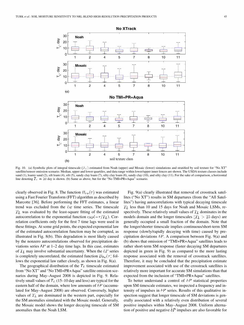
Fig. 10. (a) Symbolic plots of integral timescale �� estimated from Noah (upper) and Mosaic (lower) simulations and stratified by soil texture for “No XT”satellite/sensor omission scenario. Median, upper and lower quartiles, and data range within lower/upper inner fences are shown. The USDA texture classes includesand (1), loamy sand (2), silt loam (4), silt (5), sandy clay loam (7), silty clay loam (8), sandy clay (10), and silty clay (11). For the sake of comparison, a horizontalline denoting � � �� day is shown. (b) Same as above, but for the “No TMI+PR+Aqua” scenario.

clearly observed in Fig. 8. The function was estimatedusing a Fast Fourier Transform (FFT) algorithm as described byMarcotte [36]. Before performing the FFT estimates, a lineartrend was excluded from the time series. The timescale

was evaluated by the least-square fitting of the estimatedautocorrelation to the exponential function . Cor-relation coefficients only for the first 7 time lags were used inthese fittings. At some grid points, the expected exponential lawof the estimated autocorrelation function may be corrupted, asillustrated in Fig. 8(b). This degradation is most likely causedby the nonzero autocorrelations observed for precipitation de-viations series at 1–2 day time lags. In this case, estimatesof may involve substantial uncertainty. When the seriesis completely uncorrelated, the estimated function fol-lows the exponential law rather closely, as shown in Fig. 8(a).

The geographical distribution of the timescale estimatedfrom “No XT” and “No TMI+PR+Aqua” satellite omission sce-narios during May–August 2008 is depicted in Fig. 9. Rela-tively small values of (15–10 day and less) are typical for theeastern half of the domain, where low amounts of (accumu-lated for May–August 2008) are observed. Conversely, highervalues of are dominated in the western part, especially forthe SM anomalies simulated with the Mosaic model. Generally,the Mosaic model shows the longer decaying timescale of SManomalies than the Noah LSM.

Fig. 9(a) clearly illustrated that removal of crosstrack satel-lites (“No XT”) results in SM departures (from the “All Satel-lites”) having autocorrelations with typical decaying timescale

less than 10 and 15 days for Noah and Mosaic LSMs, re-spectively. These relatively small values of dominates in themodels domain and the longer timescales days aregenerally occupied a small fraction of the domain. Note thatthe longer/shorter timescale implies continuous/short-term SMresponse (slowly/rapidly decaying with time) caused by pre-cipitation deviations . A comparison between Fig. 9(a) and(b) shows that omission of “TMI+PR+Aqua” satellites leads torather short-term SM response (faster decaying SM departuresdepicted in green in Fig. 9) as compared to the more lastingresponse associated with the removal of crosstrack satellites.Therefore, it may be concluded that the precipitation estimateimprovement associated with use of the crosstrack satellites isrelatively more important for accurate SM simulations than thatexpected from the inclusion of “TMI+PR+Aqua” satellites.

To better understand a control of statistical propertiesupon SM timescale estimates, we inspected a frequency and in-tensity of impulses in series. Results of this qualitative in-spection suggest that longer timescale of SM deviations is gen-erally associated with a relatively even distribution of severalpositive impulses within May–August 2008. Uniform alterna-tion of positive and negative impulses are also favorable for


Fig. 11. Same symbolic boxplot arrangement as in Fig. 10, but stratified by precipitation difference amount (rounded into 5-cm bins) relative to the “All Satellites”configuration.

establishing longer decaying scales of SM deviations caused byprecipitation variations. The origin of extremely low values,which are mainly concentrated around the NE corner of the do-main in Fig. 9, are related to the series having one dominantimpulse. This major impulse (usually its magnitude exceeds 5cm day ) may cause a relatively narrow peak in the SM devi-ations series, leading to a substantial lowering of the autocorre-lation timescale .

Finally, we assessed a possible dependence of on soil tex-ture and vegetation. These environmental parameters may affect

as it can be expected from the potential evaporation controlof the SWC damping time-scale. Symbolic distributions of ,stratified by the soil texture and estimated from Noah (top) andMosaic (bottom) simulations are depicted in Fig. 10(a) for the“No XT”, and in Fig. 10(b) for the “No TMI+PR+Aqua” satel-lite omission scenarios. Although the rate of surface evapora-tion is determined by the soil texture (sandy soils dry faster thanclay), values of the timescale exhibit no systematic depen-dence on soil texture, as shown in Fig. 10. Distribution ofstratified by the vegetation type and fraction also exhibited noapparent dependence on values of these parameters. The lack ofthe relationship between the environmental parameters andcan be explained by the impact of correlations in the series.These nonzero correlations at the first two lags may result indegradation of estimates. Because a number of substantial

impulses in the series is controlled by occurrence of ratherstrong precipitation events during May–August 2008, accumu-lated amount of represent an indirect measure of intensityof these impulses. Therefore, it is reasonable to assume that theSWC damping timescale should respond to variations of the ac-cumulated . Indeed, distributions of simulated with theNoah LSM and stratified by the accumulated amount (roundedinto 5-cm bins) demonstrate systematic lowering of with theincrease of accumulated amount, as shown in Fig. 11.

Overall, these results implies that the precipitation differ-ences represented by various NRL-Blend satellite omissionscenarios (time series of ) are more important in controllingthe local temporal structure of soil water anomalies (expressedby the characteristic decaying timescale ), as compared tosoil texture properties (which define rates of surface runoff andevaporation). In other words, for LSM and precipitation forcingsettings adopted in the present study, the component of theSWC response related to precipitation variability overrides thatassociated with evapotranspiration controlled by soil textureand vegetation types and fraction.

VI. CONCLUSION

We have examined the impact of omitting certain types ofsatellites and sensors upon the performance of the NRL-Blendhigh-resolution precipitation product (HRPP). Each separate


run of the NRL-Blend omitted one or more sensors relative tothe “All Satellites” configuration. These omission experimentswere designed to examine possible types of satellite constel-lation configurations that may exist during the GPM era. Aspecific purpose was to examine the utility of the crosstrackpassive microwave (PMW) sounders in HRPP techniques. Asecond purpose was to examine the local time of observa-tion by the sun-synchronous satellite platforms (many GPMconstellation satellites will orbit in sun-synchronous orbits)affects the performance of the satellite precipitation products.The impact was examined with two methods. The first was byexamining traditional performance metrics (bias, correlation,etc.) amongst the various NRL-Blend products, where thevalidation data consisted of a dense raingauge analysis over thecentral United States, and where the validation was separatedalong the 100 W longitude line (which roughly separatesdrier, high elevation regions west of this boundary from lower,moist regions to the east). The overall performance of theNRL-Blend degrades over higher elevation areas, where PMWtechniques are known have problems. A slight but noticeabledegradation in the performance of the NRL-Blend was notedfor the case when all crosstrack sounders were removed or themorning local time crossing satellites were removed (change toequitable threat score of about 0.1 and a similar degradation inprobability of detection).

The second method consisted of examining the response ofland surface models (LSM) when the LSMs were forced withthese same HRPP precipitation datasets. Both the Noah and theMosaic LSMs, incorporated with the NASA Land InformationSystem, were used to simulate land surface and hydrologicalstates when these same NRL-Blend precipitation datasets wereused in lieu of the LIS-provided precipitation. The LSM anal-ysis examined seasonal changes in modeled soil moisture. Thebiggest impact (largest absolute values of the top 1-m SWC bi-ases) was due to the omission of either the crosstrack microwavesounders, or the morning crossing (AM) satellites. On the otherhand, omission of afternoon (PM) satellites in the NRL-Blendresulted in the smallest impact upon the soil moisture simu-lated both with the Noah and Mosaic models. Although the rel-ative magnitude of these SWC changes is small (in the 5 cmrange), these results are consistent with the raingauge-only vali-dation conclusions, suggesting the importance of the crosstrackmicrowave sounders in future GPM constellations. Since manycurrent and future GPM constellation members are operationalplatforms with NWP as a primary mission (e.g., MetOp, NPPand NPOESS), with the MHS and ATMS microwave sounderson these satellites are key instruments, there is a high likeli-hood of maintaining a robust set of high-frequency microwavesounders for the near future. On the other hand, developingmerged PMW precipitation datasets from mixtures of cross- andconically scanning sensors is a challenging task, owing to thevariable FOV and incidence angles.

Sensitivity of the 1-m SWC two-month change (duringJuly–August 2008) to variations of precipitation forcing wasalso evaluated. The largest sensitivity of SWC changes wasobserved over the LSM grid cells with sand soil texture. Atypical decaying timescale of 1-m SWC anomalies caused bycorresponding variations of precipitation forcing was evalu-

ated using linear systems theory. The timescale estimated forMay–Aug. 2008 from Noah simulations exhibited systematiclowering with an increase of the absolute value of precipitationdifference relative to the “All Satellites” scenario. These resultssuggest that precipitation differences/anomalies introduced byusing various NRL-Blend scenarios are more important in con-trolling the local temporal structure and spatial distribution of1-m SWC anomalies as compared to soil texture and vegetationtype and fraction. We propose that this control is modulatedby nonzero autocorrelations at first two lags, observed in theprecipitation difference series.

Looking ahead, GPM is currently planned to be active duringthe future NASA Soil Moisture Active Passive (SMAP) mission,and there exists a natural synergy between these two missionsthat may benefit various applications. The utilization of frequentGPM precipitation estimates over long time intervals precedingSMAP overpasses may be useful in explaining temporal vari-ations in soil moisture. SMAP data may benefit GPM with its10-km scale retrieval of soil moisture, which greatly influencesthe variable land surface emissivity, thereby leading to improve-ments to over-land precipitation retrievals.

REFERENCES

[1] G. J. Huffman, R. F. Adler, M. Morrissey, D. T. Bolvin, S. Curtis, R.Joyce, B. McGavock, and J. Susskind, “Global precipitation at one-de-gree daily resolution from multi-satellite observations,” J. Hydrome-teor., vol. 2, pp. 36–50, 2001.

[2] Y. Hong, K. L. Hsu, X. Gao, and S. Sorooshian, “Precipitation esti-mation from remotely sensed Imagery using artificial neural network-cloud classification system (PERSIANN-CCS),” J. Appl. Meteor., vol.43, pp. 1834–1853, 2004.

[3] R. J. Joyce, J. E. Janowiak, P. A. Arkin, and P. Xie, “CMORPH: Amethod that produces global precipitation estimates from passive mi-crowave and infrared data at high spatial and temporal resolution,” J.Hydrometeor., vol. 5, pp. 487–503, 2004.

[4] F. J. Turk and S. Miller, “Toward improving estimates of remotely-sensed precipitation with MODIS/AMSR-E blended data techniques,”IEEE Trans. Geosci. Remote Sens., vol. 43, pp. 1059–1069, 2005.

[5] F. J. Turk, B.-J. Sohn, H.-J. Oh, E. Ebert, V. Levizzani, and E. A. Smith,“Validating a rapid-update satellite precipitation analysis across tele-scoping space and time scales,” Meteor. Atmos. Phys., 2009, DOI:10.1007/s00703-009-0037-4.

[6] E. Ebert, C. Kidd, and J. Janowiak, “Comparison of near real-time pre-cipitation estimates from satellite observations and numerical models,”Bull. Amer. Meteor. Soc., vol. 88, pp. 47–64, 2007.

[7] G. Weymouth, G. A. Mills, D. Jones, E. E. Ebert, and M. J. Manton,“A continental-scale daily rainfall analysis system,” Austral. Meteor.Mag., vol. 48, pp. 169–179, 1999.

[8] M. R. P. Sapiano and P. A. Arkin, “An inter-comparison and validationof high resolution satellite precipitation estimates with three-hourlygauge data,” J. Hydrometeor., vol. 10, pp. 149–166, 2009.

[9] F. J. Turk, P. Arkin, E. Ebert, and M. Sapiano, “Evaluating high res-olution precipitation products,” Bull. Amer. Meteor. Soc., vol. 89, pp.1911–1916, 2008.

[10] M. Chen, W. Shi, P. Xie, V. B. S. Silva, V. Kousky, R. Higgins, and J.Janowiak, “Assessing objective techniques for gauge-based analyses ofglobal daily precipitation,” J. Geophys. Res., vol. 113, pp. 1–13, 2008,D04110.

[11] C. Surussavadee and D. H. Staelin, “Rain and snowfall retrievals athigh latitudes using millimeter wavelengths,” in Proc. IGARSS, Boston,MA, Jul. 6–11, 2008.

[12] R. Bennartz and P. Bauer, “Sensitivity of microwave radiances at85–183 GHz to precipitating ice particles,” Radio Sci., vol. 38, no. 4,p. 8075, 2003, DOI:10.1029/2002RS002626.

[13] GPM, 2008a, GPM Science Serving Society, Global PrecipitationMeasurement, NASA Goddard Spaceflight Center [Online]. Available:http://www.gpm.gsfc.nasa.gov/features/servingsociety.html

[14] GPM, 2008b, GPM Science Objectives, Global Precipitation Measure-ment, NASA Goddard Spaceflight Center [Online]. Available: http://www.gpm.gsfc.nasa.gov/science.html


[15] M. B. Ek, K. E. Mitchell, Y. Lin, E. Rogers, P. Grunmann, V. Koren,G. Gayno, and J. D. Tarpley, “Implementation of Noah land surfacemodel advances in the National Centers for Environmental Predictionoperational mesoscale Eta model,” J. Geophys. Res, vol. 108, p. 8851,2003, DOI:10.1029/2002JD003296.

[16] R. D. Koster and M. J. Suarez, “Modeling the land surface boundaryin climate models as a composite of independent vegetation stands,” J.Geophys. Res., vol. 108, pp. 2697–2715, 1992.

[17] S. V. Kumar, C. D. Peters-Lidard, J. L. Eastman, and W.-K. Tao,“An integrated high-resolution hydrometeorological modeling testbedusing LIS and WRF,” Environ. Model. Softw., vol. 23, pp. 169–181,2008.

[18] J. Gottschalck, J. Meng, M. Rodell, and P. Houser, “Analysis of mul-tiple precipitation products and preliminary assessment of their impacton Global Land Data Assimilation System land surface states,” J. Hy-drometeor., vol. 6, pp. 573–598, 2005.

[19] R. B. Grayson, A. W. Western, J. P. Walker, D. D. Kandel, J. F.Costelloe, and D. J. Wilson, “Controls on patterns of soil oisture inarid and semi-arid systems,” in Ecohydrology of Arid and Semi-AridEcosystems, P. D’Ordorico and A. Porporato, Eds. Amsterdam, TheNetherlands: Springer, 2006, ch. 7.

[20] Q. Duan and J. C. Schaake, Jr., “Total water storage in theArkansas-Red River basin,” J. Geophys. Res, vol. 108, p. 8853,2003, DOI:10.1029/2002JD003152.

[21] F. Chen and Coauthors, “Modeling of land surface evaporation by fourschemes and comparison with FIFE observations,” J. Geophys. Res,vol. 101, pp. 7251–7268, 1996.

[22] J. W. Deardorff, “Efficient prediction of ground surface temperatureand moisture, with inclusion of a layer of vegetation,” J. Geophys. Res,vol. 83, pp. 1889–1903, 1978.

[23] T. G. Smirnova, J. M. Brown, and S. G. Benjamin, “Performanceof different soil model configurations in simulating ground surfacetemperature and surface fluxes,” Monthly Weather Rev., vol. 125, pp.1870–1884, 1997.

[24] B. A. Cosgrove and Coauthors, “Real-time and retrospective forcing inthe North American Land data Assimilation System (NLDAS) project,”J. Geophys. Res, vol. 108, p. 8842, 2003, DOI:10.1029/2002JD003118.

[25] K. E. Mitchell and Coauthors, “The multi-institution North Amer-ican land Data Assimilation System (NLDAS): Utilizing mul-tiple GCIP products and partners in a continental distributed hy-drological modeling system,” J. Geophys. Res., vol. 109, 2004,DOI:10.1029/2003JD003823, D07S90.

[26] J. C. Schaake and Coauthors, “An intercomparison of soil mois-ture fields in the North American Land data Assimilation System(NLDAS),” J. Geophys. Res, vol. 109, 2004, DOI:10.1029/2002JD003309, D01S90.

[27] D. Entekhabi and I. Rodríguez-Iturbe, “Analytical framework for thecharacterization of the space-time variability of soil moisture,” Adv.Wat. Resour., vol. 17, pp. 35–45, 1994.

[28] V. Isham, D. R. Cox, I. Rodríguez-Iturbe, A. Porporato, and S. Man-freda, “Representation of space-time variability of soil moisture,” Proc.R. Soc. A, vol. 461, pp. 4035–4055, 2005.

[29] C. Yoo, S.-J. Kim, and J. B. Valdes, “Sensitivity of soil moisture fieldevolution to rainfall forcing,” Hydrol. Process., vol. 19, pp. 1855–1869,2005.

[30] R. K. Otnes and L. Enochson, Applied Time Series Analysis. NewYork: Wiley, 1978.

[31] J. S. Bendat and A. G. Piersol, Random data: Analysis and Measure-ment Procedures. New York: Wiley, 1986.

[32] S. Manabe and T. Delworth, “The temporal variability of soil wetnessand its impact on climate,” Climatic Change, vol. 16, pp. 185–192,1990.

[33] T. Delworth and S. Manabe, “The influence of potential evaporationon the variabilities of simulated soil wetness and climate,” J. Climate,vol. 1, pp. 523–547, 1988.

[34] J. K. Entin, A. Robock, K. Y. Vinnikov, S. E. Hollinger, S. Liu,and A. Namkai, “Temporal and spatial scales of observed soil mois-ture variations in the extratropics,” J. Geophys. Res., vol. 105, pp.11,865–11,877, 2000.

[35] D. Lohmann and E. F. Wood, “Timescales of land surface evapotran-spiration response in the PILPS phase 2(c),” Global and PlanetaryChange, vol. 38, pp. 81–91, 2003.

[36] D. Marcotte, “Fast variogram computation with FFT,” Comput.Geosci., vol. 22, pp. 1175–1186, 1996.

F. Joseph Turk (M’82) received the B.S. and M.S.degrees in electrical engineering from MichiganTechnological University in 1982 and 1984, respec-tively, and the Ph.D. degree in electrical engineering(specialization in microwave remote sensing) fromColorado State University in 1992.

From 1995–2008, he was affiliated with the NavalResearch Laboratory, Monterey, CA. He is currentlywith the Radar Science Group, Jet Propulsion Lab-oratory, Pasadena, CA. His research interests are inmicrowave radar and radiative transfer modeling of

clouds, precipitation and land surfaces; aircraft-based and multisatellite analysisof precipitation and cloud properties and inversion techniques; and validation ofsatellite-based precipitation datasets.

Georgy V. Mostovoy received the B.S. degree in me-teorology and climatology and the Ph.D. degree ingeography (specialization in atmospheric sciences)from Moscow State University, Moscow, Russia, in1976 and 1984, respectively.

He is currently an Assistant Research Professor inthe Geosystems Research Institute, Mississippi StateUniversity, Starkville, MS. His research interestsare numerical modeling of land surface processesand cumulus clouds and their parameterizationin weather prediction models, mesoscale weather

forecasting and validation, and air pollution modeling.

Valentine G. Anantharaj received the B.Sc. degree(physics) in 1979 from Madurai Kamaraj University,India, and the M.S. degee (meteorology) in 1990from the South Dakota School of Mines and Tech-nology. He is currently pursuing the Ph.D. degreein computation engineering at Mississippi StateUniversity, Starkville, MS.

His research interests are centered on integratingsatellite remote sensing into numerical models, tran-sitioning research results into operations, and data ac-cess and distribution which included development of

the Master Environmental Library, sponsored by the Defense Modeling andSimulations Office. He was recognized with the 2008 Research Award from theOffice of the Vice President for Research at MSU. During 2003–2005, he wasone of the recipients of the NASA EIGS Graduate Fellowship award.

soil moisture sensitivity to nrl-blend high-resolution precipitation products: analysis of...

Documents