A national laboratory of the U.S. Department of EnergyOffice of Energy Efficiency & Renewable Energy

National Renewable Energy Laboratory Innovation for Our Energy Future

Solar Advisor Model User Guide for Version 2.0 Paul Gilman Nate Blair, Mark Mehos, Craig Christensen, and Steve Janzou National Renewable Energy Laboratory

Chris Cameron Sandia National Laboratories

Technical Report NREL/TP-670-43704 August 2008

NREL is operated by Midwest Research Institute ● Battelle Contract No. DE-AC36-99-GO10337

Solar Advisor Model User Guide for Version 2.0 Paul Gilman Nate Blair, Mark Mehos, Craig Christensen, and Steve Janzou National Renewable Energy Laboratory

Chris Cameron Sandia National Laboratories

Prepared under Task No. PVB7.6201

Technical Report NREL/TP-670-43704 August 2008

National Renewable Energy Laboratory1617 Cole Boulevard, Golden, Colorado 80401-3393 303-275-3000 • www.nrel.gov

Operated for the U.S. Department of Energy Office of Energy Efficiency and Renewable Energy by Midwest Research Institute • Battelle

Contract No. DE-AC36-99-GO10337

NOTICE

This report was prepared as an account of work sponsored by an agency of the United States government. Neither the United States government nor any agency thereof, nor any of their employees, makes any warranty, express or implied, or assumes any legal liability or responsibility for the accuracy, completeness, or usefulness of any information, apparatus, product, or process disclosed, or represents that its use would not infringe privately owned rights. Reference herein to any specific commercial product, process, or service by trade name, trademark, manufacturer, or otherwise does not necessarily constitute or imply its endorsement, recommendation, or favoring by the United States government or any agency thereof. The views and opinions of authors expressed herein do not necessarily state or reflect those of the United States government or any agency thereof.

Available electronically at http://www.osti.gov/bridge

Available for a processing fee to U.S. Department of Energy and its contractors, in paper, from:

U.S. Department of Energy Office of Scientific and Technical Information P.O. Box 62 Oak Ridge, TN 37831-0062 phone: 865.576.8401 fax: 865.576.5728 email: mailto:reports@adonis.osti.gov

Available for sale to the public, in paper, from: U.S. Department of Commerce National Technical Information Service 5285 Port Royal Road Springfield, VA 22161 phone: 800.553.6847 fax: 703.605.6900 email: orders@ntis.fedworld.gov online ordering: http://www.ntis.gov/ordering.htm

Printed on paper containing at least 50% wastepaper, including 20% postconsumer waste

Executive Summary The Solar Advisor Model provides a consistent framework for analyzing and comparing power system costs and performance across the range of solar technologies and markets, from photovoltaic systems for residential and commercial markets to concentrating solar power and large photovoltaic systems for utility markets.

This manual describes Version 2.0 of the software, which can model photovoltaic and concentrating solar power technologies for electric applications for several markets. The current version of the Solar Advisor Model does not model solar heating and lighting technologies. The current version number is displayed in the software under Help, About.

Solar Advisor Model Disclaimer © 2008 National Renewable Energy Laboratory

The Solar Advisor Model is provided by the National Renewable Energy Laboratory ("NREL"), which is operated by the Midwest Research Institute ("MRI") for the Department Of Energy ("DOE"). Access to and use of the Solar Advisor Model shall impose the following obligations on the user. The user is granted the right, without any fee or cost, to use the Solar Advisor Model for any purpose whatsoever, except commercial purposes or sales, but not to modify, alter, enhance or distribute. Further, the user agrees to credit DOE/NREL/MRI in any publications that result from the use of the Solar Advisor Model. The names DOE/NREL/MRI, however, may not be used in any advertising or publicity to endorse or promote any products or commercial entity unless specific written permission is obtained from DOE/NREL/MRI. The user also understands that DOE/NREL/MRI is not obligated to provide the user with any support, consulting, training or assistance of any kind whatsoever with regard to the use of the Solar Advisor Model or to provide the user with any updates, bug-fixes, revisions or new versions. The Solar Advisor Model is provided by DOE/NREL/MRI "as is" and any express or implied warranties, including but not limited to, the implied warranties of merchantability and fitness for a particular purpose are hereby disclaimed. In no event shall DOE/NREL/MRI be liable for any special, indirect or consequential damages or any damages whatsoever, including but not limited to claims associated with the loss of data or profits, which may result from an action in contract, negligence or other tortious claim that arises out of or in connection with the access, use or performance of the Solar Advisor Model.

Microsoft and Excel are registered trademarks of the Microsoft Corporation.

i

Table of Contents Executive Summary ..................................................................................................................................... i Solar Advisor Model Disclaimer ................................................................................................................. i Table of contents ........................................................................................................................................ ii List of Tables ............................................................................................................................................... v Before you Begin ........................................................................................................................................ 1

About the Solar Advisor Model .................................................................................................1 Contacting user support .............................................................................................................2

Getting Started ............................................................................................................................................ 2 Installing and starting the software ............................................................................................2 What to do if you encounter a bug .............................................................................................3 Reviewing an existing analysis ..................................................................................................4 Creating a new analysis .............................................................................................................4 Working with files and cases .....................................................................................................5

Solar Advisor file formats ....................................................................................................6 User Interface Overview ............................................................................................................................. 6

Main window .............................................................................................................................6 Text box background colors.......................................................................................................7 Run Analysis and results buttons ...............................................................................................9

Results ......................................................................................................................................................... 9 Metrics table.............................................................................................................................10 Graphs ......................................................................................................................................14

Adding and removing sliders .............................................................................................17 Customizing graphs ...........................................................................................................18

Spreadsheets .............................................................................................................................20 Time series graphs in DView ...................................................................................................22

Waterfall graphs (CSP only) ..............................................................................................24 Exporting Data and Graphs...................................................................................................................... 25

Exporting graph and table data ................................................................................................26 Exporting graph images ...........................................................................................................27

Input Pages ................................................................................................................................................ 28 Program ....................................................................................................................................28 Environment .............................................................................................................................29 Climate .....................................................................................................................................30

Typical Meteorological Year (TMY2) ...............................................................................30 EnergyPlus Weather (EPW) data .......................................................................................31

Utility Rates .............................................................................................................................32 Financials .................................................................................................................................32 Incentives .................................................................................................................................35 Loads ........................................................................................................................................37 System: Photovoltaic ...............................................................................................................37

Configuration .....................................................................................................................38 Array ..................................................................................................................................38 Module: PV ........................................................................................................................40 Module: CPV .....................................................................................................................42 Inverter ...............................................................................................................................43

ii

Storage and BOS ................................................................................................................44 System: Concentrating Solar Power ........................................................................................44

Configuration .....................................................................................................................45 Solar Field ..........................................................................................................................45 SCA / HCE .........................................................................................................................48 Power Block .......................................................................................................................51 Storage ...............................................................................................................................54 Parasitics ............................................................................................................................58

System: Generic .......................................................................................................................58 Costs .........................................................................................................................................60

Capital costs .......................................................................................................................60 Operation and maintenance costs.......................................................................................61 Entering year-by-year O&M costs .....................................................................................62

Working with Parametric Variables ......................................................................................................... 63 Example 1: Independent parametric ........................................................................................65 Example 2: Independent parametric with linkage ...................................................................70 Example 4: Combination parametric with linkage ..................................................................79 Example 5: Review the CSP parametric analysis ....................................................................85

Working with External Workbooks and UDVs........................................................................................ 87 Overview ..................................................................................................................................88 A. Review the external workbook ...........................................................................................89 B. Define the Captured From variable .....................................................................................90 C. Create a UDV ......................................................................................................................91 D. Define the Sent To variables ...............................................................................................92 Managing UDVs, Sent To and Captured From Variables .......................................................94

Appendix 1: Levelized cost of energy (LCOE) ....................................................................................... 95 Residential and commercial LCOE .........................................................................................96 Utility LCOE ............................................................................................................................96 Real and nominal LCOE ..........................................................................................................97

Appendix 2: Cash Flow ............................................................................................................................. 98 After tax net equity cash and cost flows ..................................................................................98 State and federal taxes .............................................................................................................99 Total operating expenses........................................................................................................101 Total debt payment ................................................................................................................101 Project income (revenue and offset payments) ......................................................................102

Appendix 3: Equations for Calculated Values ..................................................................................... 102 Financials ...............................................................................................................................103 Loan Amount .........................................................................................................................103 Weighted Average Cost of Capital ........................................................................................103 PV Array ................................................................................................................................104 PV Derate ...............................................................................................................................106 PV Module .............................................................................................................................107 PV Inverter .............................................................................................................................107 CSP Solar Field ......................................................................................................................108

Solar Field Area, Solar Multiple, and Exact Area ...........................................................108 Exact Number of SCAs ....................................................................................................109 Solar Field Piping Heat Losses ........................................................................................109

iii

CSP SCA / HCE.....................................................................................................................110 HCE Optical Efficiency ...................................................................................................110 HCE Heat Losses .............................................................................................................111

CSP Power Block ...................................................................................................................112 Design Turbine Thermal Input.........................................................................................112

CSP Storage ...........................................................................................................................112 Maximum Energy Storage ...............................................................................................112 Heat Exchanger Duty .......................................................................................................113 Maximum Power To and From Storage...........................................................................113

CSP Parasitics ........................................................................................................................114 Effective tax rate ....................................................................................................................115

References ............................................................................................................................................... 116 Weather data ..........................................................................................................................116 Project economics financing ..................................................................................................116 Performance models...............................................................................................................116 CSP technology ......................................................................................................................116 TRNSYS and Excelergy ........................................................................................................117 Useful web sites .....................................................................................................................117

Index ......................................................................................................................................................... 118

iv

v

List of Tables Table 1. Current status of Photovoltaic modeling in the Solar Advisor Model .................................... 1 Table 2. Current status of Concentrating Solar Power modeling in the Solar Advisor Model ........... 2 Table 3. Description of text box background colors. .............................................................................. 9 Table 4. Variables that appear in the Metrics table for different financing types............................... 11 Table 5. Standard Graph Descriptions and Samples. ........................................................................... 16 Table 6. Graph Axis options..................................................................................................................... 20 Table 7. DView graph formats. ................................................................................................................. 23 Table 8. Hourly data variable names and explanations for CSP systems. ......................................... 23 Table 9. Hourly data variable names and explanations for PV systems. ............................................ 23 Table 10. Waterfall variable names in DView. Primary variables are shown in bold font. ................ 25 Table 11. Program options. ...................................................................................................................... 29 Table 12. Financing options for different project types. ....................................................................... 33 Table 13. Finacials page variables. ......................................................................................................... 34 Table 14. Summary of incentives and tax credits. ................................................................................. 36 Table 15. Heat transfer fluids. .................................................................................................................. 47 Table 16. Default collector types. ............................................................................................................ 49 Table 17. Default receiver types. ............................................................................................................. 50 Table 18. Receiver conditions.................................................................................................................. 50 Table 19. Power cycle reference systems. ............................................................................................. 52 Table 20. Reference system parameters. ............................................................................................... 53 Table 21. Suggested Tank Heat Losses values for different thermal storage capacities. ................ 55 Table 22. O&M cost options. .................................................................................................................... 61

Before you Begin

About the Solar Advisor Model The Solar Advisor Model provides a consistent framework for analyzing and comparing power system costs and performance across the range of solar technologies and markets, from photovoltaic systems for residential and commercial markets to concentrating solar power and large photovoltaic systems for utility markets.

Installation requirements:

• The installation file: SAM_install.exe.

• A computer running Windows Vista, XP or 2000 with at least 500 MB of free disk space.

• Microsoft® Excel if you plan to use the spreadsheet linking feature. Solar Advisor combines an hourly simulation model with performance, cost, and finance models to calculate energy output, energy costs, and cash flows. The software can also account for the effect of incentives on cash flows. Solar Advisor includes both built-in cost and performance models, and a spreadsheet interface for exchanging data with external models developed in Microsoft Excel. Most of Solar Advisor's inputs can be used as parametric variables for sensitivity studies to investigate impacts of variations in performance, cost, and financial parameters on model results.

This manual describes the current version of the software, which can model photovoltaic and concentrating solar power technologies for electric applications for several markets. The current version of the Solar Advisor Model does not model solar heating and lighting technologies. The current version number is displayed in the software under Help, About.

Solar Advisor models photovoltaic flat-plate and concentrating grid-connected systems.

Table 1. Current status of Photovoltaic modeling in the Solar Advisor Model

Technology Module Inverter Storage Balance of

System Flat-plate photovoltaic

• Single-point efficiency

• Sandia PV Array Performance Model

• CEC Performance Model

• Single-point efficiency

• Sandia Performance Model for Grid-Connected PV Inverters

• Under development

• Under development

Concentrating photovoltaic (CPV)

• Single-point efficiency

• Single-point efficiency

• Sandia Performance Model for Grid-Connected PV Inverters

• Under development

• Under development

Solar Advisor also models concentrating solar power (CSP) systems. The current version only models trough systems, future versions will model other types of CSP systems.

1

Table 2. Current status of Concentrating Solar Power modeling in the Solar Advisor Model

Technology Solar Field Collector and

Receiver PowerBlock Storage Parasitics

Concentrating Solar Power (CSP)

• Layout as multiple of design point or specified area

• List of heat transfer fluid options

• Library of collector types

• Library of receiver types and condition

• Library of power cycle types

• Thermocline • Two-tank

Storage

• Library of parameter sets for parasitic losses

The single-point efficiency models are simple representations of system components based on a size value in rated watts or kilowatts and an efficiency value. The PV single-point efficiency model also includes a simple representation of module temperature effects. The commercial models represent particular commercially available inverters and PV modules using a set of parameters based on field measurements. System components that are in development are not available in the current version of Solar Advisor.

The Department of Energy's Solar Energy Technologies Program (SETP) initially developed Solar Advisor for analysis to support the implementation of the SETP Systems Driven Approach. The model also has applications for the solar industry for planning research and development programs, and developing project cost and performance estimates. Solar Advisor is being used as part of the Solar America Initiative application and monitoring process.

Solar Advisor models system performance using the TRNSYS software developed at the University of Wisconsin combined with customized components. TRNSYS is a validated, time-series simulation program that can simulate the performance of photovoltaic, concentrating solar power, water heating systems, and other renewable energy systems using hourly resource data. TRNSYS is integrated into Solar Advisor so there is no need to install TRNSYS software or be familiar with its use to run Solar Advisor.

Contacting user support If you have any questions about Solar Advisor, please send an email to Solar_Advisor_Support@nrel.gov.

You can also find more information about the model on the Solar Advisor website.at https://www.nrel.gov/analysis/sam/.

Getting Started Installing and starting the software The following procedure describes how to install the software, open a sample file, and create a second copy of the file for reviewing inputs.

Solar Advisor comes with a set of four sample files:

• Standard PV Systems.sam

• Standard CSP Systems.sam

2

• Parametrics Example.sam

• Workbook Example.sam The sample files are located in the Samples folder. There is a backup copy of each sample file in the Backup folder. Both the Samples and Backup folders are located in the same folder as the Solar Advisor program files, which is C:\SAM unless you specify a different folder in the installation process.

Note. Solar Advisor must be installed on a local drive. The software will not work properly if it is installed on a network drive or if any of the files it uses are on a network drive.

To install Solar Advisor and start the software: 1. Download or copy the installation file, SAM_install.exe, to a convenient folder on your

computer. You can download the file at http://www.nrel.gov/analysis/sam.

2. Run the installation file and follow the installation wizard instructions.

3. On the Windows taskbar, click the Start button.

4. Click All Programs, and click to start the software. There are several ways to start the software. For example, depending on your Windows setup, you can click the shortcut on your desktop, or the command in the Start menu.

5. When you start Solar Advisor for the first time, the software prompts you to select a sample file. Each time you start the software, you must open an existing file.

To uninstall Solar Advisor: • Run the Windows Add/Remove Program tool and delete the Solar Advisor folder, which is

C:\SAM by default.

What to do if you encounter a bug Solar Advisor is under development and may occasionally fail. If you encounter a bug while using the software, Solar Advisor displays an error message giving you several options.

It is unlikely that you will encounter a bug as you work through this guide, but if you do, in the error message window, click continue application. If the message persists, click restart application to restart the software. If you cannot restart the software, contact User Support.

3

Tip. If you encounter a bug during your work, in the error message window, click send bug report. The Solar Advisor support team will receive a copy of the bug report and contact you to help resolve the problem. You can also contact the Solar Advisor support team directly by sending an email to Solar_Advisor_Support@nrel.gov.

Reviewing an existing analysis Solar Advisor allows you to review an existing analysis performed by someone else, or to create a new analysis.

Summary of steps to review an existing analysis: 1. Open the file containing the analysis.

2. Save a copy of the file to review.

3. Review graphs and tables on the Results Summary page.

4. Review input variables of interest in the input pages.

When you review an existing analysis, you can start by looking at the graphs and tables on the Results page, and then look at the assumptions on the input pages. The input pages contain variables and options that define the parameters of the analysis. The pages are grouped into three categories: Program, Environment, and System. The Program inputs define the power system type and market in which the project will operate. The Environment inputs describe the project's location, utility rates, incentives, and financing. The System inputs describe the physical characteristics of the power system.

Note. If you change the value of any input variable, the Run Analysis button appears in the navigation menu and you can no longer view the results of the previous model run. If that happens, close the file you are reviewing, and open the original file to restore the original results. The current version of Solar Advisor does not have an undo function.

Creating a new analysis You must always start an analysis with an existing file, which can either be one of the sample files packaged with the software or a file prepared in an earlier analysis. Solar Advisor does not allow you to start with a new or empty file. This approach makes it possible to start with a quick first cut of an analysis using default input values to get preliminary results, and then to refine the analysis by revising input variables as you develop a better understanding of the importance of different variables.

Summary of steps to create a new analysis: 1. Open an existing file, either a sample file or one from a previous analysis.

2. Review the input pages and modify any variables as appropriate.

3. Run the model and view results. In this step, you may need to create custom graphs to display your results in a meaningful way.

4. Refine inputs and repeat Steps 1-3 until the results are satisfactory.

4

Tip. If Solar Advisor takes more than a few seconds to display a case or graph, you can speed things up by changing the startup mode setting. To change the setting, click Settings on the File menu, and on the General tab of the Settings window, select Slow startup (fast viewing of graphs and cases).

Some advanced analyses may require sensitivity studies. For sensitivity studies, you can define one or more parametric variables or create separate cases. See Sensitivity analysis: Working with parametric variables for a description of how to set up parametric variables or use cases for a sensitivity analysis.

Other advanced analyses may require more detailed inputs than Solar Advisor provides, or the use of output from external spreadsheet models as input to Solar Advisor. For these analyses, you can link Solar Advisor to one or more external spreadsheets. Solar Advisor can use values from named ranges in Excel workbooks as input variables. Working with external workbooks and UDVs describes how to use Solar Advisor's linked spreadsheet and optional user defined variables to add detail to your analysis.

Advanced analysis options: • Define parametric variables for sensitivity studies.

• Link to external spreadsheets for detailed analysis.

Working with files and cases A Solar Advisor file contains one or more cases. A case is a complete set of input data and results that represents the cost and performance of a single system design using a particular technology in a given market. Solar Advisor displays different cases on tabs in the same way that spreadsheets are displayed in an Excel workbook. By creating more than one case in a file, you can easily compare the assumptions and results of different analysis scenarios. For example, you could use cases to compare the cost and performance of a residential photovoltaic system in several locations by defining a separate case for each location.

There are three commands that you can use to manage cases:

• Duplicate: Creates a copy of the active case, with a duplicate set of input parameters and results.

• Delete: Deletes the active case.

• Rename: Allows you to edit the name that appears on the case tab.

To view the case commands: • Click the Case menu, or, right-click a case tab.

5

Solar Advisor file formats Solar Advisor saves files in three formats: SAM, ZIP, and SCIF:

• SAM is the standard format and saves all input variables, results, weather data for each case in the file. Typical SAM files sizes range from 5 to 10 MB.

• ZIP is a compressed archive that contains the SAM file and any workbooks linked to the file. ZIP files range in size from 500 KB to 1.5 MB.

• SCIF is a compressed archive that contains only input variables for one or more cases. SCIF files range in size from tens to hundreds of kilobytes.

Solar Advisor can open files in two formats: SAM and SCIF. To open a ZIP file, use a file compression utility program.

You can import one or more cases from a SCIF file into an open SAM file by using the Import Case(s) command on the File menu.

User Interface Overview The Solar Advisor user interface organizes model input variables into pages of related variables. The navigation menu along the left side of the main window provides access to the input pages, using buttons which are presented from top to bottom in the following order:

• The Program input pages define the technology and market.

• Environment input pages contain variables that are independent of the system technology and describe the solar resource, as well as economic and financial parameters and incentives.

• Variables on the System pages describe the technology, equipment used in the system and their costs.

The buttons at the bottom of the navigation menu run the model and display results.

Main window The main window consists of a navigation menu and data page. Navigation buttons in the navigation menu select the data page to display. Data pages display results and input data. Tabs along the top of the window provide access to each case in the file. The menu bar provides access to command menus.

6

Text box background colors The background color of text boxes provides information about the data in the box. On the View menu, click View Input Type Legend to display a legend of background colors.

7

8

Table 3. Description of text box background colors.

Background color Description of variable type

White User Specified: Data that you can edit by typing in the box. Brown Parametric: The variable is a parametric variable and has more than one value. The

value in the box with the brown background is the base value of the parametric variable. Right-click the box to view all values. See Sensitivity analysis: Working with parametric variables.

Yellow CapturedFrom: The value is linked to a cell in a spreadsheet. Right-click the box to access the spreadsheet. See Working with external workbooks and UDVs.

Blue Calculated: Values that Solar Advisor calculates based on the values of other input variables. For example, in the Module page, the Power box appears with a blue background because Solar Advisor calculates the module power using values for the module size and efficiency.

Blue type font

Referenced: This value from a different input page appears as part of the text on the current page.

Green Schedule: A variable that has a different value for each year in the analysis period. For example, seven-year inverter replacement costs could be specified by defining the operation and maintenance Fixed (per year) cost variable on a schedule, with an annual payment every seven years. See Costs.

Run Analysis and results buttons Note. If you are accustomed to using Version 1.3 of Solar Advisor: The buttons described in this section replace the Results button that was at the top of the navigation menu in previous versions of the software. This new approach makes it more obvious how to view results in different formats.

The Results area of the navigation menu changes state depending on the status of input variables. Whenever you change an input value, the results area displays the red Run Analysis button, and you can no longer view results from the previous model run.

When you click the Run Analysis button, Solar Advisor calculates results, and the Results area displays three buttons: Summary, Spreadsheet, and Time Series.

For a description of the different results formats, see Results.

Results This chapter describes the Metrics table and graphs on the Results Summary page, project and case summary spreadsheets, and the time series graphs displayed in the DView data viewer.

9

To view results: • Click the Summary button to view the Results Summary page.

• Click Spreadsheet to open an Excel workbook.

• Click Time Series Graphs to open DView.

When you change the value of any input variable, Solar Advisor disables the results buttons and displays the red Run Analysis button, and you can no longer view the results of the previous model run. The current version of Solar Advisor does not have an Undo function. If you are reviewing an analysis and want to avoid accidentally modifying the file, save a copy of the file before viewing the results. (Click Save As on the File menu to save a copy of a file.)

Tip. If Solar Advisor takes more than a few seconds to display a case or graph, you can speed up the display speed by changing the startup mode setting. To change the setting, click Settings on the File menu, and on the General tab of the Settings window, select Slow startup (fast viewing of graphs and cases). The change will take effect after you restart the software.

Metrics table The variables that appear in the Metrics table depend on the system being modeled. For example, the table below on the left is for a residential system and displays fewer variables than the table on the right, which is for a utility system with IPP financing. You can right-click the Metrics table to copy its contents and paste it into a document. You can also view the same data on the Metrics Table tab of the results spreadsheet.

The Base column in the Metrics table displays results calculated from values of input variables as they appear on the input pages. The Slider column displays results calculated from the values of input variables shown on sliders: Moving a slider changes values in the Slider column (and graph), but not in the Base column. See Adding and removing sliders for more information about sliders.

10

Note. If the project or case includes parametric variables, the results in the Metrics table are for the base values of the parametric analysis. (The word "Base" in the Metrics table refers to the default slider values, not to the base value of a parametric analysis.) The Metrics table does not display the results of parametric analyses. See Working with Parametric Variables for information about parametric analyses.

The variables that appear in the Metrics table and on the Metrics Table tab in the results spreadsheet depend on the type of financing defined on the Financials page. The variables followed by an asterisk (*) in the table below are input variables from the Financials page that are included in the Metrics table for reference.

Table 4. Variables that appear in the Metrics table for different financing types.

Type of Financing Variables in Metrics Table Residential Cash Residential Mortgage Residential Loan

LCOE Net Present Value (NPV) Simple Payback kWh / kW - Year 1 Capacity Factor Annual Output - Year 1

Commercial Cash Commercial Loan

LCOE Tax Adjusted Utility Rate Net Present Value Simple Payback kWh / kW - Year Capacity Factor Annual Output - Year 1

Utility IPP Commercial Third Party System Ownership

LCOE Actual IRR Actual Min DSCR First Year PPA PPA Escalation Rate* Debt Fraction* Min Cash Flow kWh / kW - Year Capacity Factor Annual Output - Year 1

Utility IOU LCOE kWh / kW - Year 1 Capacity Factor Annual Output - Year 1

LCOE The levelized cost of energy for projects financed by cash, mortgage, or loan is the cost per unit of energy, that, when multiplied by the total energy produced and discounted to a base analysis year, is equivalent to the present value of the total life-cycle cost of the project.

For utility projects with independent power producer financing, or commercial projects with third party ownership financing, the LCOE is the cost per unit of energy, that, when multiplied by the total energy produced over the project life and discounted to the base analysis year, is equivalent to the present value of the project required revenues over the project life given a set of financing constraints defined on the Financials page.

11

For a detailed description of LCOE, see Levelized Cost of Energy (LCOE).

Note. The LCOE for the systems in the sample files includes the effects of incentives. To see what the LCOE would be with no incentives, set the sliders for all incentives to zero, and read the LCOE value in the Slider column of the Metrics table.

Net Present Value (NPV) The net present value is the present value of the after tax net equity cash flow discounted to year one using the discount rate on the Financials page plus the after tax net equity cash flow in year zero.

Simple Payback The simple payback is the time in years starting in year one of the project that it takes for the cumulative cash flow to switch from negative to positive.

The payback cash flows for each year are shown on the Cashflow tab of the results spreadsheets:

Payback Cash Flow = After Tax Cash Flow + Debt Interest Payment x (1 - Effective Tax Rate) + Debt Repayment

The cumulative cash flow for each year is:

Cumulative Cash Flow = Payback Cash Flow + Cumulative Cash Flow (of previous year)

kWh / kW - Year 1 The kilowatt-hour per kilowatt-year metric is the annual output in year one divided by the system capacity. For photovoltaic systems, the system capacity is the Array Power on the Array page. For concentrating solar power systems, the system capacity is the Rated Turbine Net Capacity on the Power Block page.

Capacity Factor The Capacity Factor is the first year annual output divided by the system capacity divided by 8,760 hours per year. The system capacity for photovoltaic systems is Array Power on the Array page, and for concentrating solar power systems is the Rated Turbine Net Capacity on the Power Block page.

Annual Output - Year 1 The annual output in year one is the number of kilowatt-hours or megawatt-hours produced by the system in its first year of operation. Note that output in subsequent years may be lower than the first year depending on the value of the degradation rate on the Array page for photovoltaic systems and on the Power Block page for concentrating solar power systems.

12

Note. You can see system's annual output on the Output graph on the results summary page, and on the cash flow tab in the results spreadsheet.

Tax Adjusted Utility Rate The tax adjusted utility rate is the Utility Rate on the Utility Rates page less state and federal taxes:

TaxAdjustedUtilityRate = UtilityRate - (UtilityRate x EffectiveTaxRate).

The effective tax rate is a single rate that includes both the state tax rate and federal tax rate.

Actual IRR, Actual Min DSCR, and First Year PPA For utility systems with IPP financing and commercial systems with third party ownership financing, the internal rate of return (Actual IRR), minimum debt service coverage ratio (Actual Min DSCR), and first year electricity sales price (First Year PPA) must meet the constraints defined on the Financials page.

Note. The revenue stream, cash flow, and loan payment streams shown in the equations below are on the Cashflow tab of the results spreadsheet.

The internal rate of return is the discount rate, IRR, that corresponds to a project net present value, NPV, of zero:

0)1( 0

1

=++

−= ∑

=

shFlowAfterTaxCaIRR

shFlowAfterTaxCavenueRequiredReNPVN

nn

nn

The debt service coverage ratio in each analysis year (DSCRn) is the ratio of operating income to expenses in that year:

nn

nnn aymentPrincipalPymentInterestPa

ostOperatingCvenueRequiredReDSCR

+−

=

In Solar Advisor, the project's debt service coverage ratio is the lowest value of the DSCR that occurs in the life of the project:

nNnDSCRDSCR

],1[min∈

=

Solar Advisor calculates the first year sales price, FirstYearPPA, by using an iterative search algorithm to find the first year sales price that, when inflated using the user-defined escalation rate, meets the minimum required IRR and the minimum required DSCR constraints, and results in a positive cash flow for each year if that is a requirement:

Find FirstYearPPA such that

Actual IRR ≥ Minimum Required IRR, and

13

Actual Min DSCR ≥ Minimum Required DSCR, and Cash Flow in Year n > 0 (when the cash flow requirement is positive)

The minimum required IRR and DSCR are user input variables on the Financials page. The positive cash flow requirement is set by a check box on the Financials page.

Utility projects with IOU financing must meet a single constraint on the internal rate of return. Solar Advisor calculates an annual revenue requirement that meets the IRR constraint.

Find FirstYearRevenueRequirement such that Actual IRR ≥ Minimum Required IRR

Min Cash Flow The minimum cash flow is the lowest positive value in the after tax net equity cash flow, which is displayed in the both Cashflow standard graph on the Results Summary page and on the Cashflow tab of the results spreadsheet.

Graphs The Graphs list on the Results Summary page includes a set of standard, pre-defined graphs that allow you to quickly view results in typical formats. Standard graphs are indicated in the Graphs list with an asterisk before the name. You can modify these graphs or create custom graphs if the standard graphs do not meet your needs.

To view standard graphs: 1. In the Graphs list, select the standard graph you want to view. Note the asterisks in the graph

names indicating that these are standard, pre-determined graphs.

2. Solar Advisor displays the graph. Note the table below the graph that displays the graph

values.

14

Tips for viewing graphs: • Adjust sliders to see the effect of changing input variables on the graph. Click Reset to return

a slider to its default position.

• Add and remove sliders using the Slider button. (See Adding and removing graph sliders.)

• Clear Autoscale before moving a slider to make graph changes more visible.

• If a graph goes off scale when you move a slider, a red arrow will appear at the top or bottom of the graph scale. Click the red arrow to automatically rescale the graph.

• To change the graph size, resize the Solar Advisor window.

• If the legend takes up too much space in a graph, clear the Legend check box to hide the legend.

• Refer to the table under the graph for exact values displayed in the graph.

• To export the data in the table to an Excel spreadsheet, click Send To Excel.

• Click Show Notes to display an editable text box to make notes about a graph. Solar Advisor associates a text box with each graph in the Graphs list.

15

Table 5. Standard Graph Descriptions and Samples.

Annual Output Total annual output versus project year. Shows the total energy produced by the system for each year of the project life.

Cashflow After-tax cash flow for each year of the project life. Red indicates negative cash flow, green indicates positive cash flow.

LCOE Real and nominal levelized cost of energy on a single graph.

Cost stacked bar

Cost of energy bar graph showing relative contribution of each project cost. The operation and maintenance (O&M) contribution is the value of all O&M cash flows discounted to year 1. The values of remaining costs are from the capital costs shown on Costs page.

Monthly Output Monthly average values of system output for each month of the year.

Monthly Energy Flow (CSP only)

Monthly average incident radiation and output at various points in the concentrating solar power system: solar field output, power block input, power block output, net electricity (after parasitic losses), net electricity (after availability factor).

16

Adding and removing sliders

A slider is a user interface element that allows you to dynamically change the value of some independent variables in graphs and see the effects on the graph. You can use sliders to see how changes in an input value impact any result that is displayed in a standard or custom graph. Solar Advisor allows many input variables and all parametric variables to be used as sliders.

Note. Moving a slider only changes the graph. It does not change the stored inputs or results.

The graphs on the results summary page of each sample file appear with a set of sliders. You can add or remove sliders by using the Sliders button. The following procedure describes how to display sliders for the Cost stacked bar chart. You can use a similar procedure to display sliders for any standard or custom graph.

To add and remove sliders for a graph: 1. Click the results summary button to display the Results Summary page.

2. Select a graph to view in the Graphs list.

3. Click Sliders to open the Slider Selection window. Solar Advisor displays a list of Available

variables and of Selected variables. The Selected variables are ones that currently appear as sliders on the Results Summary page. Available sliders are ones that are available for you to add to the list of Selected sliders.

17

4. In the Available box, select one or more variable names. Hold down the Control or Shift key

while clicking to select more than one slider.

5. Click to add the highlighted sliders to the Selected box.

You can remove sliders by selecting slider names in the Selected box and clicking . To remove all sliders, click .

6. Click OK to close the Slider Selection window. All of the variables in the Selected list appear as sliders on the Results Summary page.

Customizing graphs The Results Summary page displays two types of graphs: Standard graphs appear by default when you run an analysis and are indicated by an asterisk in the Graphs list, custom graphs are graphs that you create based on a copy of a standard graph. You cannot modify or delete standard graphs.

18

Note. When the current graph is a standard graph (indicated by a an asterisk in the graph name), only the Add button is active. When the current graph is a custom graph, the Edit, Add, and Delete buttons are active.

To create a custom graph: 1. On the Results Summary page, click Add to display the Graph Info window with a copy of

the properties of the current graph. You can save a few steps by selecting a standard graph similar to the one you want to create.

2. Solar Advisor assigns a name to the new custom graph using the name of the current graph

followed by a number indicating the number of copies that exist of the original graph.

3. Type a new name in the Name box if you want to change the graph name.

4. Select a type of graph from the Graph Type list.

5. Select variables to display on each axis of the graph. The available axes depend on the graph type. Refer to the table below for a description of graph variables.

6. Click OK to close the Graph Info window and display the graph on the Results Summary page. Solar Advisor may require a few seconds to display the graph.

To modify a custom graph: 1. On the Results Summary page, select the custom graph that you want to modify in the

Graphs list. Note that custom graph names are not preceded by an asterisk.

2. Click Edit to display the Graph Info window with a copy of the properties of the custom graph.

3. Solar Advisor assigns a name to the new custom graph using the name of the current graph

followed by a number indicating the number of copies that exist of the original graph.

19

4. Type a new name in the Name box if you want to change the graph name.

5. Select a type of graph from the Graph Type list.

6. Select variables to display on each axis of the graph. The available axes depend on the graph type. Refer to the table below for a description of graph variables.

7. Click OK to close the Graph Info window and display the graph on the Results Summary page. Solar Advisor may require a few seconds to display the graph.

Table 6. Graph Axis options.

Axis Name Description Graph TypesX Values Horizontal axis of two-dimensional graphs and contour graphs.

On three-dimensional surface plots, appears as horizontal axis perpendicular to the y-axis.

all

YValues Vertical axis of two-dimensional graphs and contour graphs. On three-dimensional surface plots, appears as horizontal axis perpendicular to the x-axis.

all

Y2 Values Second vertical axis on two-dimensional graphs. Scale displayed on right side of graph.

bar, line, stacked bar

ZValues Vertical axis of three-dimensional surface plots. Colored lines on contour plot.

surface, contour

Parameter1 Parametric variable to display on x-axis. Variable names only appear when one or more parametric variable is defined.

bar, line

Parameter2 Second parametric variable to display on x-axis. Variable names only appear in list when two or more parametric variables are defined.

bar, line

To delete a graph: 1. On the Results Summary page, select the name of the graph you want to delete in the Graphs

list.

2. Click Delete. You can only delete custom graphs from the Graphs list.

Spreadsheets Solar Advisor displays inputs and results in two different Excel workbooks:

• The case summary contains six spreadsheets containing inputs and results for a single case.

• The project summary contains a set of six spreadsheets for each case in the file.

20

Note. If the project or case includes parametric variables, the results in the workbook are for the base values of the parametric analysis. The results spreadsheets do not display the results of parametric analyses.

To open the case summary: • Click Spreadsheet in the navigation menu. If the Run Analysis button appears instead of the

results buttons, click Run Analysis to generate results. You can also open the spreadsheets on the Results menu by pointing to Case Summary, and clicking Spreadsheet.

To open the project summary: • In the Results menu, Click Project Summary.

For each case or project summary that you open, Solar Advisor creates an Excel workbook with the name of the current file and stores it in a temporary folder, which is C:\SAM\temporary by default. When you close Solar Advisor, it deletes any workbooks in the temporary folder. If you want to save the workbook, use Save As in Excel to save it to a folder other than the temporary folder.

In the project summary, the spreadsheets for each case are labeled by a number indicating the position of the case tab in the Solar Advisor main window: Case1, Case2, etc.

The six tabs for each case are Cashflow, Metrics Table, Inputs, Hourly Data, Monthly Data, and Annual Data:

• In the cash flow spreadsheet, the values in the After Tax Net Equity Cash flow row are equivalent to the values shown in the Cashflow standard graph on the Results Summary page. See Cash Flow for a description of the cash flow variables and calculations.

• The data on the Metrics Table tab are also shown on the Metrics table on the Results Summary page.

• The Inputs tab displays a list of input variable names, values, and units.

• The Hourly Data tab contains sets of 8,760 values that Solar Advisor uses to simulate the system's performance.

• The Monthly Data and Annual Data tabs contain monthly and annual averages of the hourly data.

21

Time series graphs in DView Solar Advisor displays hourly data for the current case in a built-in data viewer called DView. In DView, you can view graphs of hourly results as well as monthly and annual averages of the hourly data. DView allows you to export the data to a tab-delimited text file, and to copy graph images for use in presentations and reports.

Note. If the analysis includes parametric variables, the results in DView are for the base values of the parametric analysis. DView does not display the results of parametric analyses.

To display the graphs of time series data in DView: 1. Click Time Series Graphs. If the Run Analysis button appears instead of the results buttons,

click Run Analysis to generate results. You can also open DView on the Results menu by pointing to Case Summary, and clicking Time Series Graph.

2. In DView, click the tab for the graph format you want to view. See the table below for a

description of the different formats.

3. Select the variable or variables to view. Depending on the graph format, a list of available

variables appears either in a drop-down box or as a list of check boxes.

Tips for using DView: • For check box lists, checking a box in the leftmost column splits the graph into two and

displays the checked variable in the upper graph. Checking a box in the rightmost column displays the graph in the lower graph, or in a single graph when no boxes are checked in the leftmost column.

• Right-click a graph to export an image of the graph or a table of the data in the graph.

• Change properties of a graph, such as the graph title and labels, line colors and style, and axis bounds by right-clicking a graph and choosing Properties.

22

Table 7. DView graph formats.

Tab Name Graph Format DescriptionDMap 8,760 point data map showing entire year of hourly data in a single graph Hourly Time series line graph, use scroll bars and zoom buttons to view entire data set Daily Daily average line graph Monthly Monthly average line graph Boxplot Monthly average with daily and monthly minima and maxima Profile Average daily profiles by month PDF Probability distribution function CDF Cumulative distribution function DC Duration curve

Table 8. Hourly data variable names and explanations for CSP systems.

Variable name Units Description E_dump MW solar electric generation in excess of power plant maximum output E_gross MW gross total electric generation E_min MW solar electric generation below minimum power plant output E_net MW net electric energy production (gross parasitics) E_parasit MW total parasitics for entire system Epar_OffLine MW total offline parasitic losses Epar_OnLine MW total online parasitic losses Q_abs W/m2 absorbed energy Q_dni MW solar radiation incident on the collector Q_dump MW the amount of energy dumped (in excess of turbine and storage) Q_from_ts MW energy from thermal storage Q_gas MW gas thermal energy Input Q_hftFpHtr MW QhtfFpHtrHTF freeze protection from auxiliary heater Q_htfFPTES MW HTF freeze protection from thermal energy storage Q_nip W/m2 measured beam radiation Q_SF(MW) MW output power Q_to_PB MW energy to the power block Q_to_ts MW energy to thermal storage Q_ts_Full MW energy dumped because the thermal storage is full Q_tur_SU MW the energy needed to startup the turbine QSF_Abs MW absorbed energy for the solar field QSF_HCE_HL MW receiver heat losses for the solar field QSF_nipCosTh MW measured beam radiation cosine theta QSF_Pipe_HL MW piping heat losses for the solar field QTS_HL MW energy losses from thermal storage TIME none hour of the year TOUPeriod none time of use periods (1 through 6)

Table 9. Hourly data variable names and explanations for PV systems.

Variable Name Units Description ACPower kW AC power at inverter output, not derated AmbTemp °C ambient temperature CellTemp °C cell temperature DCPower kW DC power at array output, not derated GlobHozRad kW/m

2 global horizontal radiation

23

IncBeamRad kW/m2

incident beam radiation

IncDiffRad kW/m2

incident diffuse radiation

IncTotRad kW/m2

incident total radiation

InvEff none inverter efficiency by hour InvPartLoad none inverter part load efficiency by hour TIME hour of the year Windspd m/s wind speed

Waterfall graphs (CSP only) A waterfall graph displays groups of related variables for comparison. For concentrating solar power systems, DView displays a set of variables designed for creating water fall graphs on the Hourly, Daily, and Monthly tabs.

To create a waterfall graph: 1. Open a file containing results for a concentrating solar power (CSP) system, for example, the

sample file Standard CSP Systems.sam.

2. In the results area of the navigation menu, click Time Series Graphs. If necessary, click Run Analysis first.

3. In the DView window, click either the Hourly, Daily, or Monthly tab.

4. Clear the TIME check box and any other check boxes that might be checked.

5. Click the down arrow below the list of check boxes to scroll to the bottom of the list of variables.

There are four groups of related variables that are suitable for waterfall graphs. Each of the four groups has a primary variable: Sol_Rad_Inc_on_Coll(Qdni),

24

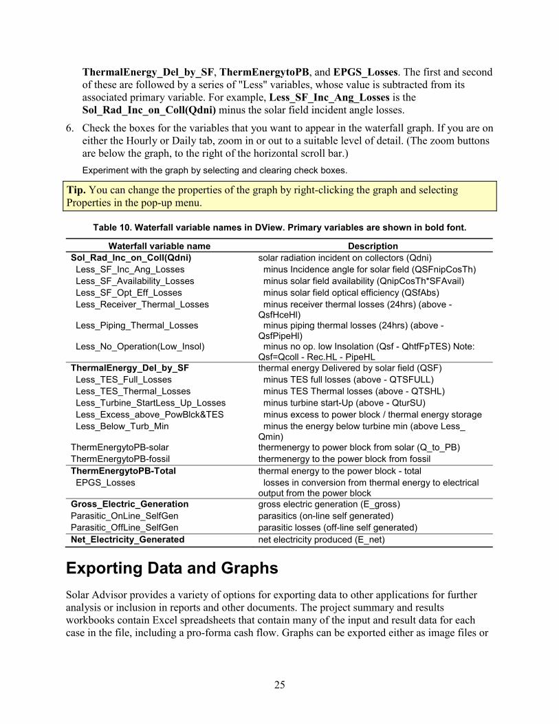
ThermalEnergy_Del_by_SF, ThermEnergytoPB, and EPGS_Losses. The first and seconof these are followed by a series of "Less" variables, whose value is subtassociated primary variable. For example, Less_SF_Inc_Ang_Losses is the Sol_Rad_Inc_on_Coll(Qdni) minus the solar field incident angle losses.

Check the boxes for the variables that you want to appear in the waterfall graeither the Hourly or Daily tab, zoom in or out to a suitable level of detail. (

d racted from its

6. ph. If you are on The zoom buttons

are below the graph, to the right of the horizontal scroll bar.) Experiment with the graph by selecting and clearing check boxes.

Tip the graph and selecting . You can change the properties of the graph by right-clickingProperties in the pop-up menu.

Table 10. Waterfall variable names in DView. Primary variables are shown in bold font.

Waterfall variable name Description Sol_Rad_Inc_on_Coll(Qdni) solar radiation incident on collectors (Qdni) Less_S minus Incidence angl d (QSFnipCosTh)

Avail)

s

Note:

F_Inc_Ang_Losses e for solar fiel Less_SF_Availability_Losses minus solar field availability (QnipCosTh*SF Less_SF_Opt_Eff_Losses minus solar field optical efficiency (QSfAbs) Less_Receiver_Thermal_Losse minus receiver thermal losses (24hrs) (above -

QsfHceHl) Less_Piping_Thermal_Losses minus piping thermal losses (24hrs) (above -

QsfPipeHl) Less_No_Operation(Low_Insol) minus no op. low Insolation (Qsf - QhtfFpTES)

Qsf=Qcoll - Rec.HL - PipeHL ThermalEnergy_Del_by_SF thermal energy Delivered by solar field (QSF) Less_TES_Full_Losses minus TES full losses (above - QTSFULL) Less_TES_Thermal_Losses minus TES Thermal losses (above - QTSHL) Less_Turbine_StartLess_Up_Losses

&TES torage e Less_

minus turbine start-Up (above - QturSU) Less_Excess_above_PowBlck minus excess to power block / thermal energy s Less_Below_Turb_Min minus the energy below turbine min (abov

Qmin) ThermEnergytoPB-solar ThermEnergytoPB-fossil

thermenergy to power block from solar (Q_to_PB) thermenergy to the power block from fossil

ThermEnergytoPB-Total thermal energy to the power block - total EPGS_Losses losses in conversion from thermal energy to electrical

n output from the power block

Gross_Electric_Generatio gross electric generation (E_gross) Parasitic_OnLine_SelfGen

d)

parasitics (on-line self generated) Parasitic_OffLine_SelfGen parasitic losses (off-line self generateNet_Electricity_Generated net electricity produced (E_net)

E nd Grap data to other applications for further

analysis or inclusion in reports and other documents. The project summary and results

e files or

xporting Data a hs Solar Advisor provides a variety of options for exporting

workbooks contain Excel spreadsheets that contain many of the input and result data for each case in the file, including a pro-forma cash flow. Graphs can be exported either as imag

25

tables of data. Solar Advisor also displays results of hourly performance calculations in graphs, or allows them to be exported as Excel spreadsheets.

Exporting graph and table data ented in graphs and shown in tables on the

d

data to a comma-separated file:

raph data in Excel.

Solar Advisor allows you to export the data represResults Summary page. You can export the data to a comma separated text file recognized by Excel and other software. You can also export the data in text or .xml format using the advanceproperties feature.

To export graph 1. Display the graph on the Results Summary page.

2. Click Send to Excel. Solar Advisor displays the g

3. Solar Advisor creates a comma-separated file in t der containing the Solar Advisor file he fol

and names it after the graph. For example, it creates the file Cost stacked bar.csv when you export the Cost stacked bar graph.

Note. el for a graph, Solar Advisor creates a new Excel file in Each time you click Send to Excthe Solar Advisor temporary folder (C:\SAM\Temporary by default). If a csv file already exists with the graph name, Solar Advisor appends (n) to the filename, incrementing n for each version of the file with the same graph name. When you close Solar Advisor, it deletes all files in the temporary folder. If you want to save the workbook, save it to a location other than the temporary folder.

To export table data: e Results Summary page.

tcut menu.

1. Display the table on th

2. Right-click the graph and click Copy on the shor

26

3. Open a text file, word-processing document or spreadsheet and paste the table data.

Advanced - To export graph data to a text, xml, or html file: 1. Display the graph on the Results Summary page.

2. Right-click the graph and click Advanced Properties on the shortcut menu.

3. In the chart editing window, click Export in the navigation tree.

4. On the Data tab, make the appropriate selections and click Copy, Save, or Send.

Exporting graph images Solar Advisor displays graphs on the Results Summary page and in DView windows. You can export images of these graphs for use in documents and reports.

To export a graph image: 1. Display the graph on the Results Summary page or in a DView window. (To open the DView

window, click Time Series Graph in the navigation menu, or click View Data on the Climate page.)

2. Right-click the graph and click Copy on the shortcut menu. In DView, choose Copy Bitmap or Copy Metafile.

27

3. Solar Advisor exports graph images as bitmaps.

4. DView allows you to export graph images as bitmaps or metafiles, and to save them as portable network graphic or metafile files. Use the metafile format when you want to scale the image of the graph after exporting it.

5. Open a word processing document or spreadsheet and paste the image by right-clicking and choosing Paste, or by pressing ctrl-V.

Input Pages This chapter describes the thirteen input pages. The navigation menu provides access to the input pages, which are categorized into three groups: Program, Environment, and System.

For a description of the calculated values (variables with blue backgrounds) on the input pages, see Equations for Calculated Values in the Appendix.

Program

28

The Program page displays options that determine the set of input variables that Solar Advisor makes available for the case. The Technology options determine the set of options that appear on the System pages, for either a photovoltaic system, concentrating solar power system, or generic system. For each Technology option, a different set of Market options is available. The Market options determine what set of financing variables appear on the Financials page.

Table 11. Program options.

Technology Available Market Options Available Financing Types

(on Financials page) Photovoltaics Central Generation • Independent Power Producer

(IPP) • Investor-owned Utility (IOU)

Commercial Buildings • Cash • Loan • Third-party Ownership

Residential Buildings • Cash • Mortgage • Loan

Concentrating Solar Power Central Generation • Independent Power Producer (IPP)

• Investor-owned Utility (IOU) Distributed Generation • Cash

• Loan • Third-party Ownership

Solar Heating and Lighting None None Generic Central Generation • Independent Power Producer

(IPP) • Investor-owned Utility (IOU)

Commercial Buildings • Cash • Loan • Third-party Ownership

Residential Buildings • Cash • Mortgage • Loan

Note. Only the Photovoltaics, Concentrating Solar Power, and Generic technology options are implemented in the current version of the software. Future versions will include Solar Heating and Lighting. Future options are disabled because they are not fully implemented in the current version of the software.

Environment The five Environment options include variables and options that describe the characteristics of the system that can be considered to be outside of the technical description or specification of the system itself. The environment options include climate, incentives, and financial parameters.

29

Climate

The Climate box in the navigation menu shows the location name for the solar resource data that Solar Advisor will use for simulation, in this case, TMY2 data for Phoenix, Arizona.

• Click the Location arrow to view a list of all available TMY2 locations.

Solar Advisor can use weather data files in two formats: Typical Meteorological Year format (TMY2) and EnergyPlus Weather format (EPW). Weather files for the United States in the new TMY3 format are available in EPW format.

Solar Advisor weather files must meet the following criteria:

• A text file in TMY2 or EPW format.

• Filename extension tm2 or epw.

• Located the Solar Advisor weather data folder, which by default is C:\SAM\Data\WeatherFiles.

Note. For more information about the weather formats, see the following websites: NREL TMY2 (typical meteorological year) format, EnergyPlus Weather file (EPW) format. See the References section for internet addresses.

Typical Meteorological Year (TMY2) The Solar Advisor Model software includes a set of TMY2 files for 239 U.S. locations. To use TMY2 data for one of these locations, select the location name in the Location list on the Climate page.

If the location you are modeling is not in the list, you can:

• Add locations to the list by adding files in TMY2 format to the SAM weather data folder.

30

• Purchase the Meteonorm database and software package, which contains climatological data for over 7,700 global weather stations and can convert the data into TMY2 format. Meteonorm can also import data in various formats and convert it to TMY2.

EnergyPlus Weather (EPW) data You can download weather data in EPW format for locations around the world at no cost from the EnergyPlus weather data website at http://apps1.eere.energy.gov/buildings/energyplus/cfm/weather_data.cfm

Note: To download TMY3 weather files in EPW format for U.S. locations, visit the EnergyPlus weather data website United States page.

To use EPW weather data: 1. Go to the EnergyPlus weather data website and navigate to the region and location you want

to model.

2. Download the EPW file for the location you are modeling. If there is not an EPW file for the location, download the ZIP file and extract the EPW file.

3. Place the EPW file in Solar Advisor's weather data folder.

The EPW file should now be visible in the Locations list on the Climate page.

Tips for downloading EPW data: • For some regions, you can download an EPW file directly for a location. For example, for

Bangladesh, you can download the data for Dhaka by right-clicking the blue square next to the word EPW for Dhaka. Be sure to save the file with the epw extension.

• For other regions, you must first download a zip file containing the EPW file and extract the

EPW file. For example, for Malaysia, you can download the data for Kuala Lumpur by right-clicking the red square next to the word ZIP for Kuala Lumpur. After downloading the zip file, you can extract the EPW file to the SAM weather files folder.

31

Utility Rates

The utility rate is the price per kilowatt hour paid to the project for electricity generated by the system. Payments and revenue from electricity sales appear in the project cash flow, but do not affect levelized cost of energy calculations. For residential and commercial projects, electricity sales are assumed to be on a net-metering basis.

The current version of Solar Advisor models a flat rate for photovoltaic and concentrating solar power systems, i.e., the same rate applies regardless of the time of day or year. It also assumes net-metering, where electricity is purchased and sold by the project at the same rate. Later versions of the software will model time-of-use rates for photovoltaic and concentrating solar power systems.

Note. The Utility Rates page for concentrating solar power (CSP) systems displays a diagram of time-of-use periods for two California utilities. The current version of Solar Advisor uses this information to determine how to dispatch storage in a CSP system, but not to determine the time dependent value of electricity. See CSP Storage for more information about storage and time-of-use periods for CSP systems.

Financials

The Financials page displays the variables that Solar Advisor uses to calculate project cash flows and other related financial metrics. Type of Financing determines which groups of variables appear on the Financials page. For example, Residential - Mortgage financing does not include the Depreciation group of variables, which is only available for the Commercial and Utility financing types. The options available in the Type of Financing list depend on the Market option on the Program page.

Note. For more details on financing options, please refer to Project economics and financing in the References section and to the financials spreadsheets on the Solar Advisor website's download page at https://www.nrel.gov/analysis/sam/download.html.

For utility projects, Solar Advisor models two types financing: independent power producer (IPP) and investor-owned utility (IOU). All utility projects are funded through a combination of debt and equity that earn revenues from electricity sales.

32

Table 12. Financing options for different project types.

Project Type Financing Options Description Residential Cash The owner pays cash in the amount of the total

installed cost in year zero of the project cash flow. Mortgage The owner pays cash for the equity portion of the total

installed cost in year zero of the cash flow, and makes an interest and principal payment in subsequent years. Interest payments are tax deductible.

Loan The owner pays cash for the equity portion of the total installed cost in year zero of the cash flow, and makes an interest and principal payment in subsequent years. Interest payments are not tax deductible.

Commercial Cash The owner pays cash in the amount of the total installed cost in year zero of the project cash flow.

Loan The owner pays cash for the equity portion of the total installed cost in year zero of the cash flow, and makes an interest and principal payment in subsequent years. Interest payments are not tax deductible.

Third Party Ownership The project earns revenues through electricity sales to cover project costs. The owner pays cash for the equity portion of the total installed cost in year zero of the cash flow, and makes an interest and principal payment in subsequent years. Depreciation, interest payments and sales tax (in year one) are tax deductible. Solar Advisor calculates a first year power purchase price that meets internal rate of return, minimum debt service coverage ratio and positive cash flow requirements.

Utility Independent Power Producer (IPP)

The project earns revenues through electricity sales to cover project costs. The owner pays cash for the equity portion of the total installed cost in year zero of the cash flow, and makes an interest and principal payment in subsequent years. Depreciation, interest payments and sales tax (in year one) are tax deductible. Solar Advisor calculates a first year power purchase price that meets internal rate of return, minimum debt service coverage ratio and positive cash flow requirements.

Investor-owned Utility (IOU) The project earns revenues through electricity sales to cover project costs. The owner pays cash for the equity portion of the total installed cost in year zero of the cash flow, and makes an interest and principal payment in subsequent years. Solar Advisor calculates a first year power purchase price that meets an internal rate of return requirement.

Note: To model a utility project with cash financing when sufficient cash is available to fund the project with no debt, choose Commercial under Buildings (grid-tied) as the market option on the Program page, and then choose Commercial - Cash for Type of Financing on the Financials page. Financing constraints do not apply to projects with cash financing.

33

Table 13. Financials page variables.

Variable Name Applicable

Market Description

Analysis Period All Number of years covered by the analysis. Typically equivalent to the project or investment life.

Inflation Rate All Annual rate of change of prices, typically based on a price index. Solar Advisor uses the inflation rate to calculate costs in the cash flows for years after year one.

Real Discount Rate All

A measure of the time value of money expressed as an annual rate. Solar Advisor uses the real discount rate to calculate the present value (value in year one) of cash flows over the analysis period and to calculate annualized costs.

[Loan] Amount All

The amount of money borrowed to cover installation expenses. Solar Advisor calculates the loan amount based on the Loan (Debt) Fraction and the Total Installed Costs on the Costs page. See Equations for Calculated Values, Financials for a description of the loan amount calculation.

Loan (Debt) Fraction All

Percentage of the total installed cost that can be borrowed. For analysis of utility IPP projects with a goal of minimizing LCOE, the loan fraction and PPA escalation rate should be adjusted so that the minimum constraining assumptions are met.

[Loan] Term All Number of years required to repay a loan. Can be more or less than the analysis period.

[Loan] Rate All Loan interest rate.

Federal Tax, State tax

Com- mercial and

Utility

Federal and state income tax rate. Applies to annual income from incentives for all projects, and to revenues from electricity sales for utility projects.

Property Tax Com-

mercial and Utility

Annual tax paid on project property, expressed as a percentage of total installed costs. Solar Advisor treats property tax as a tax-deductible operating expense for each year. In each year, the property tax expense is the property tax rate multiplied by the annualized installation cost.

Sales Tax All

A one-time tax paid in year one on equipment purchases during installation, expressed as a percentage of the taxable portion of installed costs. Solar Advisor treats sales tax as a deductible expense. The taxable portion of installed costs is defined on the Costs page.

Insurance Com-

mercial and Utility

An annual operating expense expressed as a percentage of total installed costs.

MACRS Mid-Quarter Convention

Com- mercial and

Utility

Modified Accelerated Cost Recovery System depreciation schedule offered by the Federal government and some states. This tax deduction, expressed as a percentage of the total installed cost, applies to the first years of the project life as follows: 35%, 26%, 15.6%, 11.01%, 11.01%, and 1.38%.

MACRS Half-Year Convention

Com- mercial and

Utility

Modified Accelerated Cost Recovery System depreciation schedule offered by the Federal government and some states. This tax deduction, expressed as a percentage of the total installed cost, applies to the first years of the project life as follows: 20%, 32%, 19.2%, 11.52%, 11.52%, and 5.76%.

Straight Line depreciation

Com- mercial and

Utility

A depreciation schedule offered by the Federal government and some states. This tax deduction is 20% of the of total installed cost and applies to the first five years of the project life.

PPA Escalation Rate Utility

Solar Advisor calculates an electricity sales price for each year in the project life using the PPA (Power Purchase Agreement) Escalation Rate and First Year PPA Price. For analysis of utility IPP projects with a goal of minimizing LCOE, the loan fraction and PPA escalation rate should be

34

Variable Name Applicable

Market Description adjusted so that the minimum constraining assumptions are met.

Minimum Required IRR Utility

The lowest value of the internal rate of returned required for the project to be financially feasible. The internal rate of return is the discount rate that results in a project net present value of zero.

Minimum Required DSCR

Utility The lowest value of the debt-service coverage ratio required for the project to be financially feasible. The debt-service coverage ratio is the ratio of operating income to expenses in a given year.

Positive Cashflow Utility A requirement that the annual project cash flow be positive throughout

the project life.

Incentives

The Incentives page provides a variety of options for entering most of the incentives and tax credits available to residential, commercial, and utility projects in the United States. Note that some incentive-related inputs such as state and federal depreciation and taxes are on the Financials page.

Solar Advisor only models incentives that are checked on the Incentives page. For example, the screenshot below shows a project that benefits from a 30% Federal investment tax credit with a $2,000 maximum, and a $3/W capacity based incentive provided by the utility with a $50,000 maximum. In this case, Solar Advisor will not model the state investment tax credit (25% with $1,000 maximum) because it is not checked.

35

Table 14. Summary of incentives and tax credits.

Incentive Name Type Incentive Calculation Applies in year

Investment tax credit, ITC Investment-based incentive, IBI

Investment, as percent of capital investment

Total Installed Costs ($) × Incentive Percent (%)

1

Investment tax credit, ITC Investment-based incentive, IBI

Investment, as fixed amount Amount ($) 1

Capacity-based incentive, CBI

Investment, as function of system size

Incentive Rate ($/W) × Array Size (kW), or Incentive Rate ($/W) × Rated Net Capacity (MWe)

1

Production-based incentive, PBI

Production, as function of system output

Incentive Rate ($/kWh) × Annual Output in Year n (kWh) × [1 + Escalation (%)]Year n (Annual Output is a calculated value on Results Summary page)

All, or Year 1

thru term

Note. For a description of incentives available to solar and other renewable energy projects in the United States, see the Database of State Incentives for Renewables and Efficiency at http://www.dsireusa.org.

Solar Advisor models two types of incentives: tax credits and incentive payments to the project. Tax credits can be provided by a state or federal government. Incentives are payments that can be provided by a state or federal government, utility, or other entity.

36

Incentive payments and tax credits can be either investment-based or production-based. An investment-based incentive or tax credit is a one-time payment to the project made in year one of the project cash flow that is either a fixed amount, percentage of total installed costs, or a function of system size. A production-based incentive or tax credit is an annual payment based on the amount of energy produced by the system in each year.

Incentive payments may or may not be taxable by either the Federal or state government. Solar Advisor allows you to control which incentives, if any, are taxable. To show or hide the tax details for each incentive, click Show Tax Details.

Solar Advisor applies the federal tax rate from the Financials page to any investment-, capacity-, or production-based incentives with Taxable Federal checked on the Incentives page. Similarly, it applies the state tax rate for incentives with Taxable State checked. Solar Advisor multiplies the applicable tax rate by the investment amount and adds it to each year's cash flow.

Investment tax credits and all incentive payments may or may not contribute to depreciable costs. When Basis is checked for a particular incentive, Solar Advisor subtracts the incentive amount from the depreciation basis in each applicable year of the project life.

See Cash Flow for information about how incentives affect the project cash flow.

Loads The current version of Solar Advisor does not model loads for distributed generation or off-grid markets.

System: Photovoltaic Photovoltaic systems convert global solar radiation to electricity. Solar advisor models grid-connected photovoltaic systems that consist of a photovoltaic array and inverter. The array can be made up of flat-plate or concentrating photovoltaic modules, and can be fixed, or employ single or dual axis tracking. The current version of Solar Advisor does not model battery or other types of storage, or loads for off-grid systems.

This chapter describes the system input pages that are available when the Program Technology on the Program page is Photovoltaics:

• Configuration

• Array

• Module

• Inverter

• Storage

• BOS (balance of system) The sample file, Standard PV Systems.sam, contains five cases based on photovoltaic technologies. The cases are for residential and commercial systems, and for utility systems with two types of financing. The fifth case is for a utility system using concentrating photovoltaic technology. The sample files are located in the Samples folder, which is in C:\SAM by default.

37

For a description of the Concentrating Solar Power System options see System: Concentrating Solar Power.

Configuration

The Configuration page displays options for a photovoltaic system and that determine whether the system is based on flat-plate or concentrating photovoltaic (CPV) technology, how the system is mounted, whether the system uses inverters or whether the inverters are integrated in the photovoltaic module, and whether the system includes batteries or another form of storage. Only options that are available in the current version of the software are active.

Flat plate systems use global radiation data (beam + diffuse) from the weather file, and concentrating systems use only the beam component of the radiation data.

Array

The Array page displays variables and options that describe the array layout, loss and degradation factors, and tracking and orientation of the collector.

In Layout, note that Total Modules, Array Power, and Inverter Power have blue backgrounds, indicating that Solar Advisor calculates the total number of modules, rated array power and rated inverter power values based on the values of other input variables. See Equations for Calculated Values, PV Array Layout for the equations behind these variables.

Inverters is the total number of inverters in the system. It appears here instead of on the Inverter page to make it easier to see whether the inverter capacity is adequate to meet the array's peak rated power.

Solar Advisor applies the Total pre-inverter derate factor to the output of the array, and applies the Total post-inverter derate factor to the inverter model output. You can choose to enter the derate factors in Simple mode or Detailed mode. In Detailed mode, you enter the components of the total derating factor, and Solar Advisor calculates the total value. See Equations for Calculated Values, PV Array Derate for calculation details.

The System Degradation represents an annual reduction in system output due to equipment aging. It applies to each year's derated inverter output in year two and subsequent years. When you enter the degradation rate as a single value, the degradation for each year is compounded. You can also define the system degradation using an annual schedule, which allows you to manually assign a different degradation rate to each year. One application of this approach is modeling the effect of replacing equipment within the system lifetime: You can set the system degradation to zero for the year equipment is replaced. To define an annual schedule, right-click the system degradation variable and choose Annual Schedule in the Input Type window. Note

38

that for system degradation rates entered on an annual schedule, degradation rates are not compounded annually: Solar Advisor multiplies each year's degradation rate by the first year annual output.

The graphs below show the effect of different combinations of a system derate factor of 5% and system degradation factor of 1% on the annual output of a residential, grid-connected PV system.

The Tracking options cause the software to simulate the effects of a fixed array with no tracking, an array mounted on a single-axis tracking device to follow the sun's daily east to west movement through the sky, or an array mounted with dual-axis tracking to follow both the sun's daily movement and its seasonal movement north and south.

39

The Orientation variables determine the tilt (north-south orientation) and azimuth (east-west orientation) of the array when Tracking is set to Fixed. A Tilt value of zero degrees is horizontal, and positive 90 degrees is vertical. An Azimuth value of zero is facing the equator. In the northern hemisphere, positive 90 degrees is facing due west, and negative 90 degrees is facing due east. The ground reflectance accounts for radiation incident on the array that is reflected from the ground. The Ground Reflectance variable is expressed a fraction of the global solar radiation at a given time. The typical range for ground reflectance is between 0.2 for grassy ground and 0.7 for predominantly snowy ground. Solar Advisor uses the Ground Reflectance value except for hours during which the weather data indicate that there is snow on the ground, when it uses the Ground Refl. with Snow value.

Module: PV

The Module page displays the characteristics of the performance model for flat-plate photovoltaic modules when the System setting on the Configuration page is Flat Plate.

• To select a performance model, in the Module/Array Performance Model list, click a model name.

There are three flat-plate PV performance models available in the current version of Solar Advisor:

• The Sandia PV Array Performance Model is based on empirical field measurements of module performance.

• The single-point efficiency model is a simple representation of module performance based on a single efficiency value and module area with temperature correction.

• California Energy Commission (CEC) Performance Model is based on a 5-parameter representation of a module equivalent electrical circuit and standard rating conditions supplied by module manufacturers or based on tests by an independent laboratory, such as Arizona State University Photolvoltaic Testing Laboratory.

The Sandia and CEC photovoltaic models each include a library of commercially-available modules that you can select from a list. When you select a module, Solar Advisor automatically populates the parameter variables with values for that module. To model modules that are not in either library, you can use the single-point efficiency model to define a custom module.

40

Note. The modules available in the library of commercially available modules for the Sandia and CEC performance models is determined by the modules in the databases maintained by Sandia National Laboratories and the California Energy Commission. If you download and install the CEC's CECPV model, you can read documentation of the CEC performance model that is packaged with the software. You can also download documentation of the Sandia PV performance model from the Sandia National Laboratories website. See the References section for complete citations and Internet addresses. You can also learn more about the models by exploring the module databases, which are located in the Data folder of the Solar Advisor folder (C:\SAM by default). The Sandia model database is stored in the KingDatabase folder, and the CEC model database is stored in the Modules folder. If you have questions about any of the performance models used in Solar Advisor, contact the software development team by sending an email to Solar_Advisor_Support@nrel.gov.

Sandia PV Array Performance Model • To use the Sandia model, on the Module page's Module/Array Performance Model list, click

Sandia PV Array Performance Model and select a module in the Database of Available Module Coefficients list.

The Sandia model is an empirically based model that consists of a set of curve-fit equations based on field I-V curve measurements for each module in the library. Because it is based on actual field measurements, the model has a high level of accuracy in module output predictions, but because of the time and effort required to make the field measurements, the module library in the Sandia model is less current than the CEC model library.

The first several items in the Sandia database are arrays instead of single modules. The arrays are indicated by the word "Array" in the name, which also includes the number of modules and the module type.

California Energy Commission (CEC) performance model • To use the CEC model, on the Module page's Module/Array Performance Model list, click

CEC Performance Model and select a module in the Database of Available Module Coefficients list.

The CEC performance model uses the 5-parameter model developed by the University of Wisconsin's Solar Energy Laboratory, which uses standard rating conditions data from manufacturer's module specifications and a set of semi-empirical correlation equations to predict the module's I-V curve, and thus the modules power output.

41

Single-point efficiency model for flat-plate modules • To use the single-point efficiency model, on the Module page's Module/Array Performance

Model list, click Single Point Efficiency.

The single-point efficiency model calculates module output by multiplying the total global solar radiation incident on the photovoltaic panel at a specific orientation by the module's efficiency value and making a small adjustment based on the ambient temperature.

Power is displayed for reference only and is not used in calculations. It is equivalent to the module's rated DC power, or nameplate power, and is calculated based on the equation Power (W) = Area (m2) × Efficiency × 1,000 W/m2, where 1,000 W/m2 is the incident radiation at which the module produces the nameplate power under standard test conditions.

The single-point efficiency model adjusts for temperature effects using the temperature coefficient and module construction (front and back materials) from the Module page, and ambient temperature and wind speed values from the TMY2 database. The value of Temperature Coefficient (Pmax) should be the rated maximum-power temperature coefficient from the module's technical specifications. Module Structure should describe the module's construction.

Module: CPV

The Module page displays the characteristics of the performance model for concentrating photovoltaic (CPV) modules when the System setting on the Configuration page is Concentrating.

The current version of Solar Advisor models CPV modules using a single-point efficiency model. The single-point efficiency model calculates module output by multiplying direct normal component of the solar radiation incident on the panel at a specific orientation by the module's efficiency value.

Power is displayed for reference only and is not used in calculations. It is equivalent to the module's rated DC power, or nameplate power, and is calculated based on the equation Power (W) = Area (m2) × Efficiency × 1,000 W/m2, where 1000W/m2 is the incident radiation at which the module produces the nameplate power under standard test conditions.

42

Note. The Sandia PV Array Performance model includes one CPV module, Entech 22X Concentrator(c-Si). To use the Entech module, choose Flat Plate on the Configuration page, and then on the Module page, choose Sandia PV Array Performance Model and select the Entech module from the Database of Available Module Coefficients list. The Entech module is a special case in the Sandia module database, and its coefficients have been selected to allow it to be modeled using global radiation data.

Inverter

The Inverter page displays the characteristics of the of the Inverter model. The current version of Solar Advisor includes two inverter performance models, the Sandia Performance Model for Grid-Connected PV Inverters model and the single-point efficiency model. The Sandia model allows you to choose an inverter from a list of commercially-available inverters. For inverters that are not in the list, the single-point efficiency model allows you to model custom inverters.

Sandia Performance Model for Grid-Connected PV Inverters • To use the Sandia model, on the Inverter page's Inverter Performance Mode list, click Sandia

Performance Model for Grid-Connected PV Inverters.

• Ιf your inverter is not in the list, use the single-point efficiency inverter model.

The Sandia Performance Model for Grid-Connected PV Inverters is based on laboratory measurements for a range of inverter types. The model uses a set of equations to calculate an AC power output based on a DC power input value generated by the PV module model. The inverter characteristics are described by the parameters on the Inverter page. Solar Advisor converts the model's performance curve into an equivalent part-load efficiency curve that it uses to calculate the inverter's hourly AC output.

43

Note for advanced users. The inverters available in the library of commercially available inverters is determined by the database maintained by Sandia National Laboratories. You can also download documentation of the inverter model from the Sandia National Laboratory website. See the References section for complete citations and Internet addresses. You can also learn more about the Sandia inverter performance model by exploring the files in the Inverter folder, which is located in the Data folder of the Solar Advisor folder (C:\SAM by default). If you have questions about any of the performance models used in Solar Advisor, contact the software development team by sending an email to Solar_Advisor_Support@nrel.gov.

Single Point Efficiency • To use the single-point efficiency inverter performance model, on the Inverter page's

Inverter Performance Model list, click Single Point Efficiency.

During simulation using the single-point efficiency model, Solar Advisor multiplies the photovoltaic array's DC power output by the inverter efficiency to calculate the inverter's AC power output for each hour. The inverter output cannot exceed Power, the rated inverter power. The inverter output is equivalent to the system output. See Equations for Calculated Values, PV Inverter for details.

Storage and BOS The Storage and BOS (balance of system) options for photovoltaic systems are under development and are not available in the current version of Solar Advisor.

System: Concentrating Solar Power Concentrating solar power (CSP) systems collect direct normal solar radiation and convert it to thermal energy that runs a power block to generate electricity. CSP systems are based on three types of collector technologies: parabolic troughs, linear Fresnel concentrators, dishes, and central receivers. The current version of Solar Advisor only models trough systems.

The components of a parabolic trough CSP system are the solar field, power block, and in some cases thermal energy storage system. The solar field collects heat from the sun and consists of parabolic, trough-shaped solar collector assemblies (SCAs) that focus direct normal solar radiation onto tubular heat collection elements (HCEs) or receivers. Each collector assembly consists of mirrors and a structure that supports the mirrors and heat collection elements, allows it to track the sun, and can withstand wind-induced forces. Each heat collection element consists of a metal tube with a solar radiation absorbing surface in a vacuum inside a coated glass tube.

A heat transfer fluid (HTF) transports heat from the solar field to the power block and other components of the system. Most CSP systems power blocks are based on conventional power cycle technology, using turbines to convert thermal energy from the solar field to electric energy. Some CSP systems include fossil-fuel backup systems. CSP systems that include thermal energy storage systems (TES) can generate electricity during periods of no or low solar radiation.

The concentrating solar power model in the current version of Solar Advisor is based on NREL's Excelergy software.

44

This chapter describes the system input pages that are available when the Program Technology on the Program page is Concentrating Solar Power:

• Configuration

• Solar Field

• SCA / HCE (solar collector assembly / heat collection element)

• Power Block

• Storage

• Parasitics

• Costs The sample file, Standard CSP Systems.sam, contains three cases based on concentrating solar power trough technologies. The first case represents a 100 MW baseline system with a medium temperature heat-transfer fluid and an indirect 2-tank thermal energy storage system. The second case represents a similar 100 MW system with dry cooling. The third case is a an example of a parametric study on system storage input variables and is described in Example 5: Review the CSP parametric analysis. The sample files are located in the Samples folder, which is in C:\SAM by default.

For a description of the photovoltaic options see System: Photovoltaic.

Configuration The current version of Solar Advisor allows for a single Configuration option for a CSP systems: parabolic trough systems consisting of a field of solar collector assemblies and a power block system with or without thermal energy storage. Future versions of the software will also dish Stirling, linear Fresnel, and central receiver (power tower).

Solar Field The Solar Field page displays variables and options that describe the size and properties of the solar field, properties of the heat transfer fluid, reference design specifications of the solar field, and collector orientation.

Layout and Solar Multiple Solar Advisor allows you to specify the solar field size either explicitly as an area expressed in square meters, or as a multiple of the solar field area design point. The solar field area design point, equivalent to a Solar Multiple value of one, is the solar field size required to provide sufficient thermal energy under reference ambient conditions to operate the power block at full load under standard design conditions.

45

Note. Direct Normal Radiation is a reference value that is different from the solar radiation data that Solar Advisor uses for system output calculations. The reference Direct Normal Radiation value is used to calculate the solar field area. Hourly data from the weather file shown on the Climate page determine the solar resource at the site. The Direct Normal Radiation value does depend on the system location. For example, 950 W/m2 is an appropriate value for the Mohave Desert and 800 W/m2 for southern Spain.

When Solar Advisor calculates the solar field area based on a solar multiple that you define, it scales the field area based on the ratio of your solar multiple value to one. Similarly, when you enter a solar field area, Solar Advisor scales the solar multiple based on the ratio of your solar field area value to the solar field area design point.

The Solar Multiple variable makes it possible to perform a sensitivity analysis to explore cost reductions that might result from varying the size of the solar field and power block. The second case in Standard CSP system.sam, 100 MW Baseline - Parameterized Storage, illustrates this approach, comparing levelized cost of energy for systems with different solar multiple values with and without storage. For a description of the case, see Example 5: Review the CSP parametric analysis.

Note. For explanations of the solar multiple and solar field area calculations, see Equations for Calculated Values, CSP Solar Field.

To define the solar field area using Solar Multiple: • Choose Solar Multiple under Layout and enter a value.

Solar Advisor calculates the solar field area and displays it in Solar Field Area (calculated) under Solar Multiple (Design Point).

To define the solar field area using Solar Field Area: • Choose Solar Field Area under Layout and type a value.

Solar Advisor calculates the solar multiple based on the area of the solar field and displays it in Solar Multiple (calculated).

46

Heat Transfer Fluid

The solar field heat transfer fluid (HTF) absorbs heat as it circulates through the heat collection elements in the solar field and transports the heat to the power block where it is used to run a turbine. Several types of heat transfer fluid are used for trough systems, including hydrocarbon (mineral) oils, synthetic oils, silicone oils and nitrate salts.

When you choose a heat transfer fluid in the Solar Field HTF box, Solar Advisor populates the Minimum HTF Temperature box with that oil's minimum operating temperature value. Solar Advisor will not allow the system to operate at a temperature below the minimum HTF temperature. Electric heaters maintain the fluid temperature. Solar Advisor accounts for the electric power requirement for heating on the Parasitics page.

The remaining heat transfer fluid parameters describe characteristics of the solar field that affect the performance of the heat transfer fluid. If you are unsure of what values to use for these parameters, refer to the Solar Field page for the case in Standard CSP Systems.sam.

Note. Solar field outlet temperature and solar field area data for U.S. parabolic trough power plants are available on the Troughnet website at http://www.nrel.gov/csp/troughnet/power_plant_data.html.

Table 15. Heat transfer fluids.

Name Type

Min HTF Temp

ºC

Max Operating

Temp ºC Freeze Point Comments

Solar Salt Salt 260 600 220 Caloria mineral

hydrocarbon oil

-20 300 -40 used in first Luz trough plant, SEGS I

Hitec XL Nitrate salt 150 500 120 New generation

Therminol VP-1

mixture of biphenyl and diphenyl oxide

50 400 12 Standard for current generation oil HTF systems

47

Name Type

Min HTF Temp

ºC

Max Operating

Temp ºC Freeze Point Comments

Hitec Nitrate salt 175 500 140 For high-temperature systems

Dowtherm Q Synthetic oil -30 330 -50 New generation

Dowtherm RP Synthetic oil -20 350 -40 New generation

Orientation and Tracking

The Orientation variables determine the tilt (north-south orientation) and azimuth (east-west orientation) of the array. A Tilt value of zero degrees is horizontal and positive 90 degrees is vertical. An Azimuth value of zero is facing the equator, positive 90 degrees is facing due west, and negative 90 degrees is facing due east.

The Tracking options cause the software to simulate the effects of collectors mounted on single-axis tracking devices to follow the sun's daily east to west movement through the sky, or collectors on dual-axis tracking devices to follow both the sun's daily movement and its seasonal movement north and south. When you choose Two-axis tracking, Solar Advisor disables the Collector Tilt and Collector Azimuth boxes. For two-axis tracking, Solar Advisor calculates a tilt and azimuth value for each time step based on the sun's location during that time step.

SCA / HCE The SCA / HCE parameters describe the solar collector assembly (SCA) and heat collection element (HCE). Note that the SCA is often referred to as the collector. The HCE is often referred to as the receiver. The default values for the set of SCA and HCE parameters are typical for each Collector Type and Receiver Type and Condition option.

48

Note. See http://www.nrel.gov/csp/troughnet/solar_field.html for more information on solar collector assemblies and heat collection elements. Also see relevant articles in the list of publications on the Troughnet website.

Solar Collector Assembly (SCA)

The Solar Collector Assembly (SCA) parameters are for an individually tracking component of the solar field that includes mirrors, supporting structure, and a heat collection elements or receivers. The parabolic, trough-shaped SCA mirror focuses sunlight on a line. The SCA types available in Solar Advisor represent the range of collector types either installed in currently operating systems, or used in past system designs.

Note: The solar field in the 100 MW Baseline case in the Standard CSP Systems.sam file consists of approximately 1,000 solar collector assemblies.

Table 16. Default collector types.

Name Description Location EuroTrough ET150 Torque box, galvanized steel SEGS V, Kramer Junction, California Luz LS-2 Torque-tube, galvanized steel SEGS I - VII, Kramer Junction, California Luz LS-3 Bridge truss, galvanized steel SEGS VII - IX, Kramer Junction, California Solargenix SGX-1 Organic hubbing structure,

extruded aluminum Nevada Solar One, Boulder City, Nevada

49

Receiver/Heat Collection Element (HCE)

Note. For a description of the optical efficiency and receiver heat loss calculations, see Equations for Calculated Values, CSP SCA / HCE.

The Receiver/Heat Collection Element (HCE) parameters are for an HCE that consists of a metal pipe contained in a vacuum within glass tube. The HCE runs through the focal line of the trough-shaped parabolic collector. Seals and bellows ensure that a vacuum is maintained in each tube. Anti-reflective coatings on the glass tube maximize the amount of solar radiation that enters the tube. Solar-selective radiation absorbing coatings on the metal tube maximize the transfer of energy from the solar radiation to the pipe.

Table 17. Default receiver types.

Receiver Type DescriptionLuz Cermet Original HCE design. Low reliability of seals. Schott PTR70 Vacuum Newer design with improved reliability. Solel UVAC2 Newer design with improved reliability. Solel UVAC3 The newest HCE available as of May 2008.

The performance of the HCE is highly dependent on the quality of the vacuum in the glass tube. Solar Advisor models the HCE under five different receiver conditions. Each receiver condition has a set of default optical parameter values that is appropriate for each receiver type and condition.

Table 18. Receiver conditions.

Receiver Condition DescriptionBroken glass Glass tube is damaged, increasing heat transfer between tube and

atmosphere. Fluorescent Selective coating on metal tube is compromised, reducing absorption of solar

radiation Hydrogen Hydrogen from hydrocarbon-based heat transfer fluid (e.g., mineral oil) has

permeated through metal tube into the vacuum, increasing heat transfer between metal tube and glass.

Lost vacuum Glass-to-metal seal is compromised Vacuum HCE is not damaged and is operating as designed.

50

Power Block The Power Block parameters describe the equipment in the system that converts thermal energy from the solar field or thermal energy storage system into electricity. The power block is based on a steam turbine that runs on a conventional Rankine power cycle and may or may not include fossil fuel backup. Power block components include a turbine, heat exchangers to transfer heat from the solar field or thermal energy storage system to the turbine, and a cooling system to dissipate waste heat. Solar Advisor considers the thermal energy storage system to be a separate component, which is described on the Storage page.

Turbine Parameters

The turbine parameters determine the size of the steam turbine. Solar Advisor uses the Rated Turbine Net Capacity to calculate the plant capacity factor that appears in the results summary table on the Results Summary page. The Design Turbine Gross Output determines the solar field area under standard conditions, i.e., for a Solar Multiple of one. (The Solar Multiple variable is on the Solar Field page.) The gross turbine output is typically on the order of 110% of the turbine's rated net capacity. Power Plant Availability describes plant downtime due to forced and scheduled outages. Availabilities of 94% are typical for parabolic trough systems.

The Annual Degradation represents an annual reduction in system output due to aging of equipment that applies to year two and subsequent years. When you enter the degradation rate as a single value, the degradation for each year is compounded so that the degradation rate applies to the previous year's annual output. You can also define the system degradation using an annual schedule, which allows you to manually enter a different degradation rate for each year. One application of this approach is modeling the effect of replacing equipment within the system lifetime: You can set the system degradation to zero for the year equipment is replaced. To define an annual schedule, right-click the annual degradation variable and choose Annual Schedule in the Input Type window. Note that for degradation rates entered on an annual schedule, degradation rates are not compounded annually. Power blocks in parabolic trough systems are typically well-maintained and exhibit low degradation rates. Heat exchanger fouling is the main source of system degradation, which is typically in the range of 0-0.2% per year.

51

Power Cycle

Note. For a description of the calculation for Design Turbine Thermal Input, see Equations for Calculated Values, CSP Power Block.

The Power Cycle parameters describe the steam turbine component of the power block. Solar Advisor includes six reference turbines. The reference turbines include five conventional Rankine-cycle steam turbines in a range of sizes, and one organic Rankine-cycle turbine. Conventional Rankine-cycle turbines are similar to those used in coal, nuclear, or natural gas power plants. A heat exchanger transfers energy from the solar field's heat transfer fluid to generate steam that drives the turbine. The organic Rankine-cycle turbine operates on the same principle as the conventional turbine, but uses an organic fluid, typically butane or pentane, to run the turbine instead of water.

Table 19. Power cycle reference systems.

Reference System

Approximate Solar Field Size Range

m2

Approximate Operating

Temperature ºC

Suggested Modeling Application

APS Ormat 1 MWe 300C

10,000 300 Organic Rankine-cycle power block

Nexant 450C HTF - 450 High-temperature heat transfer fluid (molten salt)

Nexant 500C HTF - 500 High-temperature heat transfer fluid (molten salt)

SEGS 30 MWe Turbine 180,000 - 230,000 300 - 400 Typical applications SEGS 80 MWe Turbine 460,000 - 480,000 400 Typical applications Siemens 400C HTF 400 High-temperature heat

transfer fluid

The Turb. Part Load Therm to Elec power cycle parameters F0, F1, ..., F4 are coefficients for a set of equations used to model the turbine cycle's thermal to electric energy conversion

52

efficiencies. Solar Advisor automatically chooses the correct coefficients when you select a turbine in Ref System. You should not modify these parameters unless you are familiar with the underlying equations, which calculate the power block's electric output as a function of the power block's thermal input.

Note. The five Turb. Part Load Elec to Therm coefficients are used to calculate conversion efficiencies of storage and fossil backup equipment, whose parameters are defined on the Storage page.

Solar Advisor uses Cooling Tower Correction factors F0, F1, ..., F4 and Temperature Correction Mode to calculate a temperature correction factor for each hour in the simulation. The temperature correction factor is used in the turbine cycle thermal to electric conversion efficiency equations. Note that for dry cooling, ambient conditions have a more significant impact on the turbine cycle efficiency than for wet cooling. The current version of Solar Advisor does not model advanced parabolic trough power systems with hybrid wet-dry cooling. The temperature correction options are:

• Wetbulb basis uses wet bulb temperature data from the weather file

• Drybulb basis uses dry bulb temperature data from the weather file

• For no temperature correction, set all five Cooling Tower Correction parameters F0 ... F4 to zero

The variables Max Over Design Operation, Turbine Start-up Energy, and Minimum Load are expressed as a fraction of the design point. Solar Advisor calculates the value of each of these parameters by scaling the values relative to the turbine design capacities on the Power Block page and the solar field reference ambient conditions on the Solar Field page. For example, a Turbine Start-up Time of 0.5 hrs and Turbine Start-up Energy of 0.2 would require that the turbine run for 30 minutes at 20% load during startup. A Max Over Design Operation value of 1.15 allows the turbine to run at up to 15% over turbine design gross output.

When you choose a turbine from the reference system library, Solar Advisor changes the values of the Power Cycle variables. The following table of shows the power cycle parameters for the standard reference systems. Note that you can use any value for the Rated Turbine Net Capacity and Design Turbine Gross Output variables, Solar Advisor will use the reference system parameters with the rated and design turbine parameters.

Table 20. Reference system parameters.

Parameter Name SEGS 30 SEGS 80 APS ORC Nexant

450 Nexant

500 Siemens

400 Rated Turbine Net Capacity 30 80 1 100 100 50 Design Turbine Gross Output 35 89 1.160 110 110 55 Design Turbine Thermal Input 93.3 235.8 5.600 278.0 269.9 147.2 Design Turbine Gross Efficiency

0.3749 0.3774 0.2071 0.3957 0.4076 0.3736

Max Over Design Operation 1.15 1.15 1.15 1.15 1.15 1.15 Minimum Load 0.15 0.15 0.15 0.15 0.15 0.15 Turb. Part Load Therm to Elec F0

-0.0571910 -0.0377260 -0.1593790 -0.0240590 -0.0252994 -0.0298

Turb. Part Load Therm to Elec F1

1.0041000 1.0062000 0.9261810 1.0254800 1.0261900 0.7219

53

Turb. Part Load Therm to Elec F2

0.1255000 0.0763160 1.1349230 0.0000000 0.0000000 0.7158

Turb. Part Load Therm to Elec F3

-0.0724470 -0.0447750 -1.3605660 0.0000000 0.0000000 -0.5518

Turb. Part Load Therm to Elec F4

0.0000000 0.0000000 0.4588420 0.0000000 0.0000000 0.1430

Turb. Part Load Elec to Therm F0

0.0565200 0.0373700 0.1492050 0.0234837 0.0246620 0.044964

Turb. Part Load Elec to Therm F1

0.9822000 0.9882300 0.8521820 0.9751230 0.9744650 1.182900

Turb. Part Load Elec to Therm F2

-0.0982950 -0.0649910 -0.3247150 0.0000000 0.0000000 -0.563880

Turb. Part Load Elec to Therm F3

0.0595730 0.0393880 0.4486300 0.0000000 0.0000000 0.467190

Turb. Part Load Elec to Therm F4

0.0000000 0.0000000 -0.1256020 0.0000000 0.0000000 -0.130090

Storage A thermal energy storage system (TES) stores heat from the solar field in a liquid medium. Heat from the storage system can drive the power block turbine during periods of low or no sunlight. TES is beneficial in many places where the peak demand for power occurs after the sun has set. Adding TES to a parabolic trough system allows the collection of solar energy to be separated from the operation of the power block. For example, a system might be able to collect energy in the morning and use it to generate electricity late into the evening.

In direct systems, the heat transfer fluid itself serves as the storage medium. In indirect systems, a second medium stores the heat with heat transfer from the HTF to the storage medium accomplished through heat exchangers. The TES system consists of one or two tanks, pumps to circulate the liquids, and depending on the design, heat exchangers. Solar Advisor models two types of TES systems: thermocline and two-tank. A thermocline system stores both the hot and cold storage medium in one tank. The zone in the tank where hot and cold fluids meet is called a thermocline. The storage tank in a thermocline system contains low-cost filler materials such as sand and rock. A two-tank system consists of a hot tank to store heat from the solar field, and a cold tank to store the cooled storage medium after the power block has extracted its energy.

Note. For more information on thermal energy storage systems for parabolic trough systems, see http://www.nrel.gov/csp/troughnet/thermal_energy_storage.html.

Thermal Energy Storage (TES)

54

To model a thermocline (one tank) or two tank system, choose the appropriate option in Thermocline or Two-Tank TES and the enter the number of hours of storage the system must provide in Equiv. Full Load Hours of TES.

Tip. An increase in the hours of thermal storage requires a commensurate increase in the solar multiple in order to minimize the levelized cost of energy for the system. The 100 MW Baseline - Parameterized Storage case in Standard CSP Systems.sam illustrates this relationship. See Example 5: Review the CSP parametric analysis for a description of the case.

When the storage medium in Storage Fluid Number is different than the heat transfer fluid on the Solar Field page, Solar Advisor models an indirect system and assumes that the TES system includes a heat exchanger. The value of Heat Exchanger Duty determines the rate at which energy can be stored in the tank. To model a direct system that uses the heat transfer fluid as the storage medium, choose the same fluid for Storage Fluid Number on the Storage page and for Solar Field HTF on the Solar Field page. For direct systems, Heat Exchanger Duty on the Storage page is inactive because no heat exchanger is required.

The two Turbine - TES Adjustment values are typically close to or slightly less than one and depend on the turbine type shown in Ref System on the Power Block page. You can use the default values provided in the sample files.

The Maximum Power to Storage and Maximum Power From Storage variables are related to the Design Turbine Thermal Input variable on the Power Block page, which also appears on the Storage page. The value of these variables is often close to or equal to the design turbine thermal input value. Solar Advisor calculates these values based on the heat exchanger duty, the storage size and the turbine design.

Note. For a description of the maximum power to and from storage and maximum energy storage variables, see Equations for Calculated Values, CSP Storage.

When the Initial Thermal Storage value is zero, Solar Advisor assumes that the storage system starts (in the first hour of the annual simulation) cold. A non-zero number indicates that the system starts with a partially or fully charged storage tank.

Table 21. Suggested Tank Heat Losses values for different thermal storage capacities.

System Description Hours of Thermal Storage

0 3 6 9 12 15100 MW 2-Tank Indirect VP-1/Nitrate Salt

0 0.62 0.96 1.23 1.56 1.87

200 MW 2-Tank Indirect VP-1/Nitrate Salt

0 1.0 1.61 2.21 2.81 3.56

200 MW 2-Tank Direct Hitec Salt

0 0.34 0.64 0.93 1.24 1.52

200 MW Thermocline Hitec Salt

0 0.25 0.51 0.70 0.96 1.21

55

Solar Advisor can model thermocline (one tank) TES systems that include sand and quartzite as filler material in the tank. In such systems, quartzite (rock) typically serves as the primary material, and sand serves as the secondary material to fill gaps between the primary material. This design reduces the amount of high-cost liquid storage medium required by the system. Using primary rock or sand typically replaces 50% to 60% of the tank volume. Using rock as a primary material and sand as a secondary material can replace 75% of the tank volume. The Thermocline Temp Degradation value is typically 25% of the difference between the hot and cold storage medium temperatures. For example, if the temperature difference is 100ºC, the degradation value should be 25ºC. Alternatively, you can define Thermocline Temp Degradation as a parametric variable, and use Solar Advisor to find the optimal value for the value. For Thermocline Efficiency Adj for TES and Thermocline Output Adj for TES, you can use the default values provided in the sample files, typically one or slightly less than one.

Note. In the current version of Solar Advisor the filler material options for two-tank systems are inactive.

Thermal Storage Dispatch Controls

The thermal storage dispatch controls are coefficients for a set of equations that model the timing of releases of energy from the thermal energy storage system to the power block. When the system includes thermal energy storage, Solar Advisor can use a different dispatch strategy for up to six different time-of-use (TOU) periods. The TOU period schedule is defined on the Utility Rates page.

56

Solar Advisor decides whether or not to operate the power block based on how much energy is stored in the TES and the values of the Thermal Storage Dispatch Controls parameters. You can define when the power block operates for each of the six TOU periods. For each hour in the simulation, if the power block is not already operating, Solar Advisor looks at the amount of energy that is in thermal energy storage at the beginning of the hour and decides whether it should start the power block. For each TOU period, there are two targets for starting the power block: one for periods of sunshine, and one for period of no sunshine.

The Turbine Output Fraction for each TOU period determines at what load level the power block runs using energy from storage during that TOU period. The load level is a function of the Turbine Output Fraction, and Design Turbine Thermal Input and the five Turb Part Load Elec to Therm factors on the Power Block page.

For each TOU period, during periods of sunshine, the power block at the load level for that TOU period only when the available storage is equal to or greater than the product of the Storage Dispatch Fraction (with Solar) and Maximum Energy in Storage. Similarly, during periods of no sunshine, the power block only runs when the available storage is equal to or greater than the product of Storage Dispatch Fraction (without Solar) and Maximum Energy in Storage.

By setting the thermal storage dispatch controls parameters, you can simulate the effect of a clear day when the operator may need to start the plant earlier in the day to make sure that the storage is not filled to capacity and solar energy is dumped, or of a cloudy day when the operator may want to store energy for later use in a higher value TOU period.

For systems with fossil-fuel backup, Fossil Fill Fraction defines the solar output level at which the fossil backup will run during each hour of a specific TOU period. For example, a fossil fill

57

fraction of 1.0 would require that the fossil backup operate to fill in every hour during a specified TOU period to 100% of design output. In that case, during periods when solar is providing 100% output, no fossil energy would be used. When solar is providing less than 100% output, the fossil backup operates to fill in the remaining energy so that the system achieves 100% output. For a fossil fill fraction of 0.5, the system would use energy from the fossil backup only when solar output drops below 50%.

Parasitics The Parasitics page displays parameters describing losses due to parasitic electrical loads, such as drive motors, electronic circuits, and pump motors. Solar Advisor includes a set of default parasitic parameters for a range of solar trough power systems. Choose a Solar Field option that is the same or similar to the system you are modeling. Solar Advisor will automatically adjust the total parasitic load to match the size of the solar field you are modeling.

The Cooling Tower Operation Mode determines whether the cooling tower fan operates at 100% or 50% of its rated capacity. Most cooling towers switch between 50% and 100% operating mode. Use the Cooling Tower at 50% or 100% for a system with a single cooling tower. Use Cooling Tower parasitics a function of load when the system design includes multiple cooling towers run.

Note. See Equations for Calculated Values, CSP Parasitics for a description of the parasitic loss calculations.

System: Generic The generic system model is a basic representation of a conventional fossil-fuel power plant. The Generic technology option makes it possible to compare analyses of photovoltaic and concentrating power systems to a base case conventional fossil fuel plant in the residential, commercial and central generation markets.

Solar Advisor displays a different set of System categories on the navigation menu depending on the Program options. This section describes the System options when the Program Technology is Generic:

The parameters for the Generic system are for a simple model of a fossil fuel power plant. Unlike the photovoltaic and concentrating solar power models, the generic model is not based on an hourly simulation engine. The first year annual output of the generic plant is based on a simple equation using the four System variables: Nameplate Capacity, Capacity Factor, Availability, and Derate.

58

The First Year Annual Output is calculated using the following equation:

Equation Variable

Solar Advisor Variable Units Description

EFirstYearOutput First Year Annual Output kW The generic system's total output in the first year,

before annual degradation applies.

ENamePlate Nameplate Capacity % The rated capacity of the generic system.

FCapacityFactor Capacity Factor %

The expected net generated electricity over one year (8760 hours) divided by the electricity that could have been generated at continuous full rated power over the year. Base load plants typically operate at capacity factors of about 90%, with capacity factors of less than 100% due to curtailed output. Load following plants and peaking plants will have lower capacity factors.

FAvailability Availability %

The number of hours per year that the generic system is able to produce electricity divided by the number of hours in one year (8760 hours). Availability factors of less than 100% are typically due to plant down time for maintenance and repair.

FDerate Derate %

A derating factor applied to the generic system rated capacity to account for output reductions caused by inefficiencies in the system from wiring losses or other causes.

The Annual Degradation represents an annual reduction in system output due to equipment aging. that applies to year two and subsequent years. When you enter the degradation rate as a single value, the degradation for each year is compounded so that the degradation rate applies to the previous year's annual output. You can also define the system degradation using an annual schedule, which allows you to manually enter a different degradation rate for each year. One application of this approach is modeling the effect of replacing equipment within the system lifetime: You can set the system degradation to zero for the year equipment is replaced. To define an annual schedule, right-click the annual degradation variable and choose Annual Schedule in the Input Type window. Note that for degradation rates entered on an annual schedule, degradation rates are not compounded annually.

The heat rate determines the cost of fuel reported as Fuel O&M Expense in year one of the project cash flow on the Results Summary page. Solar Advisor uses the heat rate to calculate the first year fuel cost as follows:

Equation Variable

Solar Advisor Variable Units Description

CFirstYearFuel Fuel O&M Expense (reported for Year 1 in the project cash flow)

$/yr The total cost of fuel for year one of the project cash flow.

CCostOfFuel Cost of Fuel (from the Costs page)

$/MMBTU The rated capacity of the generic system.

59

FHeatRate Heat Rate MMBTU/MWh The generic system's efficiency,

or number of MMBTU of heat required to produce one MWh of electricity.

EFirstYearOutput First Year Annual Output kW The generic system's total

electricity output in the first year, before annual degradation.

Costs The Costs page provides access to all system costs. Project cost input data in Solar Advisor are divided into two main categories: capital and operation and maintenance (O&M) costs. Capital costs are further categorized into direct and indirect costs described below. Solar Advisor uses the variables on the Costs page and the financial and incentives parameters to calculate the project cash flow and other cost metrics reported on the Results Summary page.

The boxes with white backgrounds are values that you can edit. Boxes with blue backgrounds contain calculated values that Solar Advisor displays for your information. Solar Advisor automatically recalculates values in blue boxes when you change the value of related variables. Numbers in blue font are values taken from other input pages.

Note: The costs in the sample files are intended to illustrate Solar Advisor's use. The cost data are meant to be realistic, but not to represent actual costs for a specific project. Actual costs will vary depending on the market, technology and geographic location of a project. Because of price volatility in solar markets, the cost data in the sample files is likely to be out of date. For more information, see the Solar Advisor Model website at https://www.nrel.gov/analysis/sam/cost_data.html.

Capital costs The capital costs represent expenses associated with the purchase of equipment and services for the project. Note that financial parameters and tax rates appear on the Financials page.

A direct capital cost represents an expense for a specific piece of equipment or installation service:

• For concentrating solar power systems, direct capital costs are expressed as dollars per area of solar field ($/m2), dollars per power block rated capacity ($/MWe), or dollars per maximum thermal energy storage capacity ($/MWht) displayed on the Storage page. The solar field area and power block rated capacities are displayed on the navigation menu.

• For photovoltaic systems, direct module and inverter costs are expressed either as dollars per rated Watt of capacity or dollars per unit. The module cost per capacity is expressed in terms of the module's DC rated power, which is shown on both the Module page and Array page. The inverter cost per capacity is expressed in terms of the inverter's AC rated power, which is shown on the Inverter page. The storage cost variable is disabled because the current version of Solar Advisor does not model storage for photovoltaic systems. BOS, or balance-of-system costs are equipment costs that cannot be assigned to either the module or the inverter, and may include such costs as mounting racks, junction boxes, and wiring. Installation costs are the labor costs associated with installing the equipment.

60

• For central generation systems, the contingency cost is a percentage of the sum of direct costs to account for expected uncertainties in the direct cost estimates.

An indirect cost is typically one that cannot be identified with a specific piece of equipment or installation service, and may include all other costs that are built into the price of the system, such as profit, overhead, and shipping costs. Depending on the purpose of your analysis, you may decide to distribute profit among the direct cost categories or include them as a single value in an indirect category.

• For residential and commercial systems, the indirect costs are divided into two categories. Miscellaneous costs may include profit, and costs such as overhead (including marketing), design, permitting, or shipping. Solar Advisor calculates Sales Taxes by applying the sales tax rate from the Financials page to the percentage of the total direct costs that you specify.

• For central generation systems, indirect costs include three categories. Engineer, Procure, Construct costs may include costs associated with design and construction of the project. Project, Land, Miscellaneous costs may include real estate and other project costs. Solar Advisor calculates Sales Taxes by applying the sales tax rate from the Financials page to the percentage of the total direct costs that you specify.

Solar Advisor uses the total installed cost, which is the sum of direct and indirect costs, to calculate the cash flow, levelized cost of energy, and other output metrics. How you assign costs to each capital cost category does not affect the total installed cost, so you can choose to distribute costs as is most appropriate for your analysis.

Operation and maintenance costs Operation and Maintenance (O&M) costs represent expenditures on equipment and services that recur each year throughout the project's life after the system is installed. Solar Advisor allows you to enter O&M costs in three ways: Fixed (per year), fixed (per capacity), and variable (per production).

Table 22. O&M cost options.

O&M Cost Category Units DescriptionFixed (per year) $ Annual fixed first year cost. Fixed (per capacity) $/kW-yr Annual first year cost proportional to the system size in kW, where

the system size for concentrating solar power systems is Rated Turbine Net Capacity on the Power Block page, and for photovoltaic systems is Array Power (in kWdc) on the Array page. For CSP systems, fixed costs typically include all recurring costs except for water-related costs.

Variable (per production)

$/MW-h Annual first year cost proportional to the calculated system production for that year in MWh. For CSP systems, variable costs typically include cost of chemicals, water purchases, and chemical treatment of water.

Solar Advisor uses the first year O&M cost input variables to calculate O&M costs in year one of the project cash flow. The first year O&M cost, annual inflation rate on the Financials page, and Escalation Rates for each O&M cost category determine the O&M cost in subsequent years. You can use the escalation rate to represent an expected annual increase in O&M cost above the annual inflation rate.

61

Note. For information on water consumption and other operation and maintenance costs and requirements for concentrating solar power (CSP) systems, see the Troughnet website: http://www.nrel.gov/csp/troughnet/power_plant_systems.html. For information on operation and maintenance costs for photovoltaic systems, see the California Energy Commission's online Distributed Energy Resource guide http://www.energy.ca.gov/distgen/economics/operation.html.

Entering year-by-year O&M costs If your analysis assumes that O&M costs occur in specific years throughout the project life, you can enter annual O&M costs on a year-by-year basis, either by typing values by hand, or by importing them from an external spreadsheet. Solar Advisor adds these annual costs to the costs you specify using the first year O&M variables on the cost page. Note that for cash flow and other calculations, Solar Advisor will add other costs for that year to the O&M cost that you enter. Solar Advisor calculates the other costs based on first year costs and the inflation rate and any escalation rates.

To enter year-by-year operation and maintenance costs: 1. On the Costs page, right-click the First Year box for the O&M cost category for which you

want to specify year-by-year costs. Solar Advisor displays an Input Type window for the variable.

2. In the Input Type window, click Annual Schedule (nominal dollars).

3. For each year in which there is an O&M cost, type a value in nominal (or current) dollars for that year.

4. Click OK to return to the Costs page.

62

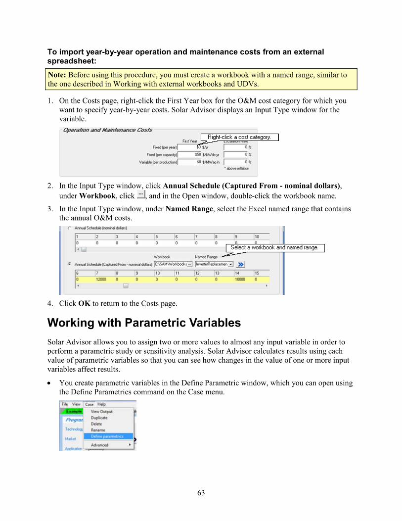
To import year-by-year operation and maintenance costs from an external spreadsheet:

Note: Before using this procedure, you must create a workbook with a named range, similar to the one described in Working with external workbooks and UDVs.

1. On the Costs page, right-click the First Year box for the O&M cost category for which you want to specify year-by-year costs. Solar Advisor displays an Input Type window for the variable.

2. In the Input Type window, click Annual Schedule (Captured From - nominal dollars),

under Workbook, click , and in the Open window, double-click the workbook name. 3. In the Input Type window, under Named Range, select the Excel named range that contains

the annual O&M costs.

4. Click OK to return to the Costs page.

Working with Parametric Variables Solar Advisor allows you to assign two or more values to almost any input variable in order to perform a parametric study or sensitivity analysis. Solar Advisor calculates results using each value of parametric variables so that you can see how changes in the value of one or more input variables affect results.

• You create parametric variables in the Define Parametric window, which you can open using the Define Parametrics command on the Case menu.

63

• The Define Parametrics window allows you to identify the input variables that you want to use in the parametric analysis, assign values to the variables, and to define relationships between the variables. You can use the window to create as simple or as complex an analysis as is appropriate for your needs.

There are three types of parametric variables in Solar Advisor. Independent Parametrics include parametric variables that are not associated with any other variables. In the example shown above, the Loan (Debt) Fraction and Federal ITC Percent variables are assigned to the independent parametrics group for an analysis that might investigate how changes in the debt-equity ratio and Federal tax credit impact the levelized cost of energy when those two variables are not related to each other. Assign parametric variables to the independent group when your analysis includes a single parametric variable, or two or more parametric variables that are not related to each other.

Combination Parametrics is a group of parametric variables that are related, but not dependent on each other. Assign parametric variables to a combination parametrics group when you want the parametric variables to appear on the same results graphs and tables. In the figure above, Azimuth and Tilt are in Combination Parametric1 to make it possible to plot a surface graph of system output versus array tilt and azimuth.

Linkages include parametric variables whose values are dependent on those of other parametric variables. One member of each linkage group must also be a member of either the independent parametrics group or of a combination parametrics group. In the figure above, Location is linked to Tilt, which is also a member of Combination Parametrics1. This variable assignment makes it possible to link array tilt values to particular locations (climates) to model a range of systems in different locations whose array tilt angle is equal to the location's latitude.

When you define the values of a parametric variable, you must define one of the values as the base value. Solar Advisor displays results based on this value in the output summary table on the Results Summary page, and resets sliders to this value when you click the slider's Reset button. Solar Advisor indicates the base value of a parametric variable with an asterisk and in bold font.

64

Overall steps for parametric analysis: 1. Define one or more parametric variables.

2. Run simulations.

3. Customize a graph or use sliders to view sensitivity analysis results.

This section walks you though five sensitivity analysis examples. You can step through the procedures to familiarize yourself with the mechanics of the Define Parametrics window and with the process of setting up custom graphs to view results from a parametric analysis.

The first four examples describe the cases in the sample file Parametrics Examples.sam and cover the mechanics of setting up the four types of parametric variable groupings: independent, independent with linkage, combination, and combination with linkage.

The fifth example is a description of a CSP parametric analysis in Standard CSP Systems.sam and illustrates the relationship in a concentrating solar power system between the solar multiple, hours of thermal energy storage, and the levelized cost of energy.

To familiarize yourself with parametric variables, you can either follow the instructions for the procedures in each example below to create your own file, or open the sample file and review the inputs as you read.

Example 1: Independent parametric This example illustrates the use of the independent parametric group. The independent group is useful for analysis that includes either a single parametric variable, or two or more parametric variables that are not related to each other.

Does the rule of thumb for optimal photovoltaic array orientation "due south at latitude tilt" apply to a residential photovoltaic system in Boulder, Colorado? To answer this question, we will define Tilt as an independent parametric variable and assign it a range of values. Solar Advisor will calculate the complete set of results for the system using each array tilt angle value. To answer the question, we will examine graphs of annual output and LCOE to find the optimal array orientation.

Note. The following procedure begins with the sample file Standard PV Systems.sam, and walks through the process of setting up an independent parametric group, running SAM, and then examining graphs of the results. The first case in the sample file Parametrics Examples.sam is a complete analysis based on this example.

Define Tilt as an independent parametric variable: 1. Open Standard PV Systems.sam. The file should be in the Solar Advisor Samples folder,

which is C:\SAM\Samples by default.

65

2. On the File menu, click Save As and choose a name for the file, such as Parametric Examples A.sam.

3. Rename the residential case: right-click the Residential Flat Plate System tab, click Rename on the shortcut menu, and type "Example 1 - Independent Parametric" in the Rename Case window.

4. Delete the remaining cases in the file: right-click each tab and click Delete on the shortcut

menu.

When you finish deleting the cases, the file should contain a single case. Deleting the other cases will make your file less cluttered as you add more cases.

5. On the Climate page, choose CO Boulder.tm2 in the Location list.

Notice that the View Results button turned red and changed to Run Analysis, indicating that you changed the value of an input variable.

6. On the Case menu, click Define parametrics to open the Define Parametric window.

7. In the Define Parametric window, under Independent Parametrics, click Add Variable.

8. In the Add Variable window, scroll to the Array section of the list and click Tilt to define it as a parametric variable.

66

The Add Variable window displays a list of all Solar Advisor variables that you can define as parametric variables. The variables are grouped into the same categories that appear on the main window's Navigation menu.

9. Click OK to return to the Define Parametric window.

10. In the Define Parametric window, under Independent Parametrics, Click Edit Values. The Tilt box should have a green background indicating that it is active.

11. In the Edit Variable window, under Specify Range, type the numbers 0 in Minimum, 10 in Increment, and 6 in # of Intervals.

12. Click Update Values.

Solar Advisor displays a list of the values that you have assigned to the parametric variable in the table under Enter Values. In this case, the minimum value of the tilt variable is 0, and there are seven values ranging from 0 to 60 degrees in increasing increments of 10 degrees.

67

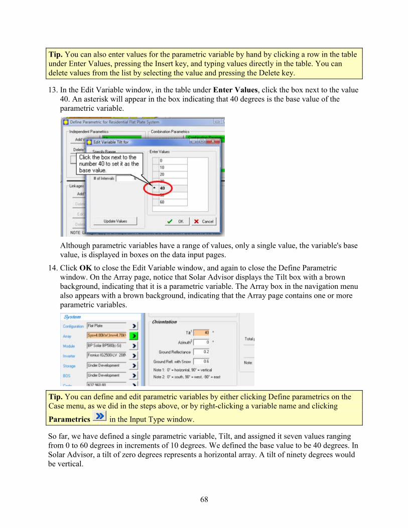
Tip. You can also enter values for the parametric variable by hand by clicking a row in the table under Enter Values, pressing the Insert key, and typing values directly in the table. You can delete values from the list by selecting the value and pressing the Delete key.

13. In the Edit Variable window, in the table under Enter Values, click the box next to the value 40. An asterisk will appear in the box indicating that 40 degrees is the base value of the parametric variable.

Although parametric variables have a range of values, only a single value, the variable's base value, is displayed in boxes on the data input pages.

14. Click OK to close the Edit Variable window, and again to close the Define Parametric window. On the Array page, notice that Solar Advisor displays the Tilt box with a brown background, indicating that it is a parametric variable. The Array box in the navigation menu also appears with a brown background, indicating that the Array page contains one or more parametric variables.

Tip. You can define and edit parametric variables by either clicking Define parametrics on the Case menu, as we did in the steps above, or by right-clicking a variable name and clicking

Parametrics in the Input Type window.

So far, we have defined a single parametric variable, Tilt, and assigned it seven values ranging from 0 to 60 degrees in increments of 10 degrees. We defined the base value to be 40 degrees. In Solar Advisor, a tilt of zero degrees represents a horizontal array. A tilt of ninety degrees would be vertical.

68

Run the simulation and view results 1. Click Run Analysis.

2. If the Inverter Size Issue window appears, click Run All. The message indicates that the inverter's rated capacity is slightly less than the array's rated capacity, which for the purposes of this exercise, is not a problem.

3. In the Information window, note that the number of TRNSYS simulations is equal to the number of values we assigned to tilt. Solar Advisor will perform a complete simulation for each tilt value.

4. Click Yes to start the simulations.

After running a simulation for each tilt value, Solar Advisor displays the Results Summary page. Note that the LCOE and other metrics that appear in the Base column of the Output summary table are calculated using the base value of each parametric variable. In this case, we set the base value of Tilt to 40 degrees, so the LCOE and other metrics reflect that value. The cash flow and other results in the project summary (Project summary on the View menu) also reflect the parametric variable's base value.

5. Because we defined Tilt as a parametric variable, Solar Advisor creates a set of new standard graphs in the Graphs list. The new graphs are Annual Output vs Tilt, LCOE vs Tilt, and Cost stacked bar vs Tilt.

6. In the Graphs list on the Results Summary page, click *LCOE vs Tilt.

7. Save the file.

The results of this parametric analysis show that given the assumptions for this project, an array tilt of 40 degrees (from the horizontal) results in the highest system annual output in kWh for tilt values of between 0 and 60 degrees. Thus, the optimal value of tilt is 40 degrees, which is what the rule of thumb suggests for Boulder, whose latitude is approximately 40 degrees north.

69

Note: You can also use sliders to examine the impact of Tilt on different results. For example, you could add a slider for the tilt variable to the Cashflow graph to explore how changes in the array tilt affect the cash flow. See Creating and using graph sliders for a description of sliders.

Example 2: Independent parametric with linkage This example illustrates the use of the linkage parametric group, which is useful for parametric analyses involving one or more variables whose value depends on that of other variables. This example also demonstrates how to define a non-numeric variable as a parametric variable.

What would the annual output of a residential photovoltaic system be in different locations, assuming that the array tilt angle for each location is equal to the location's latitude? To answer the question, we will compare the annual output of a system for three locations by linking the numeric variable Tilt, expressed in degrees, with the text variable, Location, expressed as a place name.

Note. If you did not follow the procedure in Example 1: Independent Parametric, you can start with the file Parametrics Examples.sam, which should be in the Solar Advisor folder (C:\SAM\Samples by default).

Link the independent parametric variable Tilt to Climate: 1. Open the file that you created in Example 1 (or the sample file Parametrics Examples.sam).

2. Create a copy of the Example 1 - Independent case: right-click the Residential Flat Plate System tab, click Duplicate on the shortcut menu.

3. Rename the new case to "Example 2 - Independent with Linkage" Right-click the case tab

and click Rename on the shortcut menu.

4. On the Case menu, click Define parametrics to open the Define Parametric window.

5. On the Array page, right-click the Tilt variable box.

6. In the Tilt Input Type window click Parametrics .

7. In the Define Parametric window, under Linkages, click Add Variable.

8. In the Add Variable window, click Tilt and Location. (Scroll up to the Climate section to find the Location variable.)

70

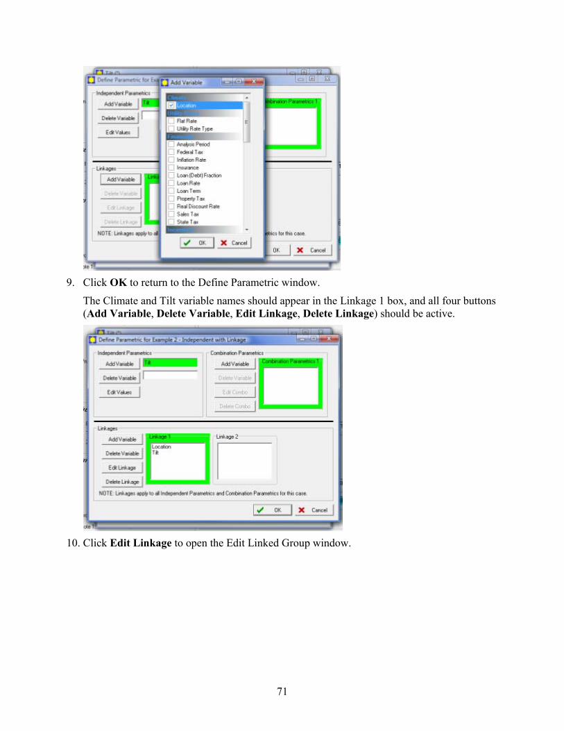
9. Click OK to return to the Define Parametric window.

The Climate and Tilt variable names should appear in the Linkage 1 box, and all four buttons (Add Variable, Delete Variable, Edit Linkage, Delete Linkage) should be active.

10. Click Edit Linkage to open the Edit Linked Group window.

71

Notice that the climate variable values appear in the Edit Linked Group window in drop-down boxes because they are non-numeric values. Solar Advisor has assigned CO Boulder.tm2 to each of the seven Module Tilt values that we created in Example 1 because we have not yet assigned values to the Climate variable.

For this example, we are going to use only three locations, Boulder, Seattle, and Newark.

11. Use the arrow in each of the first three rows of Location column, to select CO Boulder.tm2, WA Seattle.tm2, and NJ Newark.tm2.

12. Type a new value in the Tilt column for each location: CO Boulder 40, WA Seattle 48, and NJ Newark 41. Set CO Boulder as the base value.

13. Use the Delete key to delete the remaining rows. You may need to delete each cell in the table individually. If necessary, you can use the Insert key to add a row.

14. Click OK to close all of the parametric windows and return to the Array page.

72

So far, we have defined a linked parametric group, and assigned it two variables, Location and Tilt. The Location variable is also defined as an independent parametric variable. In the next procedure, we will run the simulation to create a set of results for each of the values.

Run the simulation and view results: 1. Click Run Analysis.

2. If the Inverter Size Issue window appears, click Run All. The message indicates that the inverter's rated capacity is slightly less than the array's rated capacity, which for the purposes of this exercise, is not a problem.

3. In the Information window, note that the number of TRNSYS simulations is equal to the number of linked parametric variables. Solar Advisor will perform a complete simulation for each of the three locations we specified.

4. Click Yes to start the simulations. When Solar Advisor finishes calculations, the Results Summary page appears.

5. In the Graphs list, click *Annual Output Vs Location.

6. Save the file.

The graph shows the annual output predicted for the three locations at tilt equals latitude.

Notes: You can also use sliders to examine results for the three locations. For example, you could add a slider for the Location variable to the Cashflow graph to explore the cash flow for each location. See Creating and using graph sliders for a description of sliders.

Example 3: Combination parametric This example illustrates the use of the combination parametric group, which is useful for parametric analyses involving related variables that you want to appear in a single graph, but whose values are not dependent on each other.

In Example 1: independent parametric, we found that for Boulder, Colorado, the array tilt suggested by the photovoltaic system design rule of thumb "due south at latitude tilt" is correct. Is the due south array azimuth suggestion also correct for Boulder? To find out, we will define a combination parametric group that contains the both the Tilt and Azimuth variables. Adding Tilt and Azimuth to a combination group will allow us to create a contour graph of system output

73

versus tilt and azimuth. We can then use the graph to find the values of both tilt and azimuth that result in the highest annual system output.

Define Tilt and Azimuth as combination parametric variables: 1. Open Standard PV Systems.sam. The file should be in the Solar Advisor Sample folder,

which is C:\SAM\Samples by default.

2. On the File menu, click Save As and choose a name for the file, such as Parametric Examples B.sam.

3. Rename the residential case: right-click the Residential Flat Plate System tab, click Rename on the shortcut menu, and type "Example 3 - Array Orientation" in the Rename Case window.

4. Delete the remaining cases to reduce clutter in your file by right-clicking each case's tab and

clicking Delete on the shortcut menu.

5. On the Climate page, change the location to CO Boulder.tm2.

6. On the Array page, right-click the variable box for Tilt.

7. In the Tilt Input Type window click Parametrics .

8. In the Define Parametric window, under Combination Parametrics, click Add Variable.

9. In the Add Variable window, scroll to the Array section and click both Azimuth and Tilt to define them as parametric variables.

74

10. Click OK to return to the Define Parametric window. Notice that the tilt and azimuth

variables appear in the Combination Parametrics1 box. Solar Advisor created a second box named Combination Parametrics2 to allow for additional parametric groups.

11. In the Define Parametric window, click Edit Combo to display the Edit Group window. The CombinationParametrics1 box should have a green background indicating that it is active.

12. In the Edit Group window, under Azimuth, click Edit Values to open the Edit Variable window. The window displays the current values of each variable.

13. In the Edit Variable window, under Specify Range, type -30 for Minimum, 10 for Increment and 6 for # of Intervals, and click Update Values. Solar Advisor displays a list of the values that you assigned to the parametric variable in the table under Enter Values. In this case, the minimum value of the azimuth is -30 degrees, with seven values ranging from -30 to +30 degrees in increasing increments of 10 degrees.

14. In the Edit Variable window, in the table under Enter Values, scroll to the row containing the value 0, and click the box next to the value. An asterisk will appear in the box indicating that 0, or due south, is the base value of the azimuth parametric variable.

75

15. Click OK to return to the Edit Group window.

16. In the Edit Group window, under Tilt, click Edit Values and specify a range with a minimum of 0, increment of 10 and number of intervals of 6.

17. Set 40 as the base case. Boulder's latitude is approximately 40 degrees North.

18. Click OK to return to the Edit Group Window. Solar Advisor displays the azimuth and tilt

variables and their values side by side so that you can quickly check their values.

76

Tip. In this example, using the same number of values for the two variables will help the appearance of the graph we will create later by ensuring that the tilt and azimuth axes have the same number of ticks. When deciding on a number of values to use for Combination Parametrics, keep in mind the graph's appearance.

19. Click OK to close the parametric variable windows and return to the Array page. On the Array page, notice that the tilt and azimuth variable boxes appear with brown backgrounds, indicating that they are parametric variables. The Array box in the navigation menu also appears with a brown background, indicating that the Array page contains one or more parametric variables.

Tip. You can define and edit parametric variables by either using the Define parametrics command on the Case menu, as we did in the steps above, or by right-clicking a variable name

and clicking Parametrics in the Input Type window.

20. Save the file.

Run the simulation and view results: 1. Click Run Analysis.

2. If the Inverter Size Issue window appears, click Run All. The message indicates that the inverter's rated capacity is slightly less than the array's rated capacity, which for the purposes of this exercise, is not a problem.

Solar Advisor displays an Information window telling you the number of TRNSYS simulations and approximate time the analysis will take, in this case 49 simulations. Because

77

we assigned seven values each to azimuth and tilt, the analysis requires 7 × 7 = 49 simulations Solar Advisor will perform a complete simulation for each combination of tilt and azimuth we specified.

3. Click Yes to start the simulations. When Solar Advisor finishes calculations, the Results Summary page appears.

4. When the results are complete, save the file.

After running the simulations, Solar Advisor displays the Results Summary page. Solar Advisor calculates values that appear in the results summary table using the base value of each parametric variable in the analysis. In this case, we set the base value of the array tilt variable to 40 degrees and of the array azimuth to 0 degrees, so the LCOE and other metrics in the table reflect a system with an array at latitude tilt pointing due south. The cash flow, time series data, and other results in the project summary (Project summary on the View menu) all reflect the parametric variable's base value.

In order to view the impact of array orientation on system output, we will create a contour graph of system output versus tilt and azimuth.

5. On the Results Summary page, click Add to open the Graph Info window.

6. In the Graph Info window, type "Array Orientation" in the Name box, select Contour in

Graph Type, Azimuth in X Values, Annual Output (kWh) in ZValues, and Tilt in YValues.

7. Click OK to create the graph.

8. Solar Advisor makes the calculations necessary to display the custom graph and then displays it on the main window. The custom graph name also appears in the list of graphs.

9. Check Legend under the graph to display a color key on the graph. You can right click the

graph to copy an image of the graph to the clipboard for use in other applications.

10. Save the file.

78

As you can see on the contour graph (and in the table under the graph), the orientation that results in the highest annual output is a tilt of 40 degrees and azimuth of -10 degrees. Note that the optimal azimuth is ten degrees east of south, not due south as the rule of thumb suggests. This may be due to late afternoon effects of sun setting over mountains and summer afternoon thunderstorms. The optimal tilt, on the other hand, is about 40 degrees north, approximately the latitude of Boulder, Colorado, and consistent with the rule of thumb.

Example 4: Combination parametric with linkage This example illustrates the use of both a combination parametric group and a linked group, which is useful when variables in a combination group that you want to appear in a single graph are also related to other variables.

What is the optimal array orientation for three different locations? In Example 3, we assigned the azimuth and tilt variables to a combination parametric group to plot system output versus tilt and azimuth on a contour graph. The graph showed that the optimal array tilt angle for the residential photovoltaic project in Boulder, Colorado was what we expected, 40 degrees north, close to Boulder's latitude. The optimal azimuth for Boulder, on the other hand, was about 10 degrees east of south, not the standard due south. Because the rule of thumb "array tilt equals latitude" was valid for Boulder, we assume in this exercise that it is also true for all three locations. In this example, we will use the same combination group of azimuth ant tilt, and link the tilt variable to location, which will allow us to plot a graph of array output for a range of azimuth variables for each of the three locations on a single graph.

When you perform a parametric analysis with more than one variable, the number of calculations can become very large. In Example 3, Solar Advisor performed 49 simulations for each combination of 7 azimuth values and 7 tilt values. If we were to repeat that analysis for three locations instead of one, the number of calculations increases to 147 (49 combinations times three locations). Some analyses with larger numbers of variables and parametric values simulation run times can become impractically long. Linking related parametric variables can help minimize run times by avoiding unnecessary simulations. In this example, by linking the

79

location variable to the latitude variable, Solar Advisor only simulates combinations of tilt and latitude values that make sense (assuming that we only want to simulate systems whose array tiangle equals the location's latitude). For example, linking tilt to location will ensure that Solar Advisor does not

lt

run a simulation using Seattle's radiation data and Boulder's 40 degree latitude

1. ple 3 - Combination case, right-click the tab

If y ile cs Examples.sam, which should be in the Solar Advisor folder (C:\SAM by

2. bination with Linkage." (Right-click the case's tab

3. ow should appear with the variables Azimuth and Tilt in the Combination Parametrics1 box.

for the array tilt.

Define Location and Tilt as linked parametric variables: Open the file that you created in Example 3 and create a copy of the Example 3 - Combination case. To create a copy of the Examand then click Duplicate on the shortcut menu.

ou did not follow the procedure in Example 3, you can start with the same case in the fParametridefault).

Rename the new case to "Example 4 - Comand click Rename on the shortcut menu.)

On the Case menu, click Define Parametrics. The Define Parametric wind

4. Under Combination Parametrics, select Tilt and click Delete Variable.

Under Combina5. tion Parametrics, click Add Variable and in the Add Variable window,

6. Parametric window. Azimuth and Location appear in the Combination Parametrics1 box.

click Location.

Click OK to return to the Define

80

7. Under Linkages, click Add Variable. 8. In the Add Variable Window, click Location and Tilt. (Scroll down to the Array section to

find the Tilt variable).

9. The Location and Tilt variable names should appear in the Linkage 1 box.

10. Click Edit Linkage to open the Edit Linked Group window.

Notice that the Location variable values appear in the Edit Linked Group window in drop-down boxes because they are non-numeric values. Solar Advisor has assigned CO Boulder.tm2 to each of the Module Tilt values that we created in Example 3 because we have not yet assigned values to the Location variable.

11. Assign the following values to the Location and Module Tilt variables: Boulder 40, Los Angeles 34, and Newark 41 and delete the remaining rows so that only three rows appear in the table. Set Boulder as the base value. Select location names from the drop-down lists, and use the Delete and Insert keys to delete and insert rows.

12. Click OK to return to the Define Parametric window, and again to return to the main

window.

Create a custom clustered bar graph to display the results: 1. On the Results Summary page, in Graphs, click *Annual Output vs Location. in the Add

to open the Graph Info window.

2. Click Add to open the Graph Info window.

81

3. In the Graph Info window, type "Array Orientation vs Location" in the Name box, in Graph Type click Bar, in X Values click Location, in YValues click Annual Output, and in Parameter1 click Azimuth.

4. Click OK to create the new graph.

Solar Advisor makes the calculations necessary to display the custom graph and then displays it on the main window.

5. The legend displays the Azimuth value for each bar color: the dark green bar is for -30

degrees, or 30 degrees east of south. The red bar is for 30 degrees west of south, and the light green bar is for zero degrees, or due south.

82

Tip. If the location labels do not appear on the graph, try resizing the main window to enlarge the graph. You can also clear the Legend check box below the graph to hide the legend and make more room for the graph.

The graph shows that the optimal array azimuth (in terms of total annual output) is different for each city. You can use the graph's advanced properties to change the y-axis scale to see the differences more clearly.

6. Double-click the graph to display the chart editing window.

7. In the navigation tree, under Axis, click Left Axis, and on the Scales tab, change the

minimum value from 0 to 5500.

83

Tip. You can change other properties of the graph in the chart editing window. For example, to display the legend below the graph, in the navigation tree, click Legend and on the Position tab, click Bottom.

8. Click OK to return to the chart editing window, and click Close to return to the Results Summary page.

9. Save the file.

From the clustered bar graphs, you can tell which array azimuth provides the maximum annual output for each location. For Boulder, which is located just east of the Rocky Mountain foothills, where mountains and thunder clouds to the west often shade the city in the late afternoon, the optimal array orientation is away from the mountains: -10 degrees, or 10 degrees east of south, represented by the yellow bar. For Los Angeles, located on the Pacific coast and exposed to frequent morning fog, orienting the array to maximize exposure to the afternoon sun maximizes system output: the optimal orientation is 10 degrees west of south, represented by the orange bar. For Newark, the optimal array orientation is zero degrees, or due south, represented by the light

84

green bar. The graphs also show that the difference in output for array orientations between ten degrees west of south and ten degrees east of south is relatively small.

Example 5: Review the CSP parametric analysis This section describes the fourth case in the file Standard CSP Systems.sam, 100 MW Baseline - Parameterized Storage. The case illustrates how the variations in the Solar Multiple variable and the number of hours of thermal energy storage affect the system's levelized cost of energy. For a description of the variables used for this analysis, see the Solar Field page and Storage page descriptions. If you are not familiar with Solar Advisor's parametric variables, you may want to read the Sensitivity analysis: Working with parametric variables. Examples 1 through 4 above describe the details of working with parametric variables, this example describes the analysis of the Concentrating Solar Power (CSP) system solar multiple and hours of thermal electric storage.

For a CSP trough system with no storage, the optimal levelized cost of energy typically occurs at a solar multiple of between 1.4 and 1.5. Because a trough system only operates at its design point (solar multiple of one) for a very few hours of the year, over-sizing a system (solar multiple greater than one) allows the system to operate closer to the design point for more hours of the year, which results in a reduction in the average levelized cost of energy. However, there is a trade-off between the increased cost of the larger system and the increased electric energy output that it produces: As the size increases beyond a certain point, the higher cost outweighs the benefit of the higher electricity output. This analysis investigates where that point occurs for systems with different amounts of storage capacity.

Note that an analysis for such a plant design should account for any energy that might be dumped during periods when the solar field produces more energy than the power block requires. Typically, as long as the amount of dumped energy is less than about 10-15% of the new energy resulting from the oversized system, you can reduce the LCOE by increasing solar field size.

To review the CSP parametric analysis on solar multiple and thermal energy storage: 1. Open the file Standard CSP Systems.sam.

2. Click the 100 MW Baseline - Parameterized Storage tab.

3. On the Case menu, click Define Parametrics to open the Define Parametrics window.

4. Under Combination Parametrics, click Edit Combo to open the Edit Group window.

Solar Advisor displays a list of values for each of the parametric variables. The Solar Multiple values range from 1 to 3.5 in increments of 0.25. The Equiv. Full Load Hours of TES values range from 0 to 12 in increments of 3.

85

5. Solar Advisor must simulate one system for each combination of values for the two

variables. In this case, 11 values × 5 values = 55 simulations.

Note that the base value of each variable appears in bold. Although parametric variables have a range of values, only a single value, the variable's base value, is displayed in boxes on the data pages.

6. Click Cancel to return to the Define Parametric window.

7. Under Linkages, click Edit Linkage to open the Edit Linked Group window.

8. The Equivalent Full Load Hours of TES and Tank Heat Loss variables are linked, so Solar

Advisor will only simulate systems using values of each of the two variables that are in the same row. For example, for 0 hours of storage, Solar Advisor will use 0 for the tank heat loss. For 3 hours of storage, the tank heat loss will be 0.62, etc.

9. Click Cancel to return to the Define Parametric window.

10. In the Define Parametric window, click Cancel to return to the main window.

86

11. On the Results Summary page, select the Parametric Storage Results graph if it is not already visible.

Solar Advisor displays a graph of the real levelized cost of energy versus the Solar Multiple. Each line in the graph represents a number of hours of thermal energy storage from the list we saw in the list of parametric values for the Equivalent Full Load Hours of TES variable (0, 3, 6, 9, and 12 hours of storage). Because the hours of storage variable is linked to the tank heat loss variable, each line also represents a tank heat loss value. We saw those values in the Edit Linked Group window: 0, 0.62, 0.96, 1.23, 1.56.

For the no storage case (the dark green line, zero hours of storage), the lowest levelized cost of energy occurs at a solar multiple of 1.5. The solar multiple represents the area of the solar field. An increase in the solar multiple results in a larger solar field (and thus higher area-dependent installation costs), but also in a higher electrical energy output. The interaction of these factors causes the levelized cost of energy to decrease as the solar multiple increases from 1, but at some point (1.5 in the no storage case), the cost increase overwhelms the benefit of the increased electric energy output, and the levelized cost of energy begins to increase with the solar multiple.

Working with External Workbooks and UDVs You can connect any input variable in Solar Advisor to a named cell a Microsoft Excel workbook. This feature allows you to use external spreadsheet-based cost and performance models to generate values for Solar Advisor input variables. Because Solar Advisor can both import values from workbooks and export values to them, you can use the result of a spreadsheet calculation as the value of one input variable that depends on the value of other input variables. UDVs are user-defined input variables that can also share values with external workbooks.

This chapter uses an example to describe how to prepare an Excel workbook to share data with Solar Advisor, set up input variables in Solar Advisor to send and receive values from Excel, and define user-defined variables. The chapter uses examples that require the samples file Standard

87

PV Systems.sam, and User Guide Workbook Example.xls, which are copied to the Solar Advisor folder when you install the software.

Overview A CapturedFrom variable is an input variable whose value Solar Advisor imports from a cell in an external workbook. A Captured From variable is indicated in the Solar Advisor user interface by a text box with a yellow background.

A SentTo variable is an input variable whose value Solar Advisor exports to a named cell in a workbook. You can view a list of Sent To variables in the current case by clicking SentTo variables on the View menu.

A UDV, or user-defined variable, is a variable that you can create to store values in Solar Advisor and to enhance analyses involving external spreadsheets. Solar Advisor allows you to create one or more user-defined variables on each input page. The software stores values of user-defined variables but does not use them in any internal calculations. You can connect user-defined variables, like other input variables, to external spreadsheets. For example, you could use a user-defined variable connected to an external spreadsheet to convert units of input variables. You could also use user-defined variables to pass values between an external spreadsheet-based cost or performance model and Solar Advisor.

Keep the following points in mind when working with external workbooks and user-defined variables:

• When Solar Advisor calculates results, it keeps a copy of the spreadsheet open in the background and actively exports and imports values during calculations. If a Solar Advisor calculation changes the value of a Sent To variable and Excel uses the value of that Sent To variable to calculate a Captured From variable's value, Solar Advisor will display results based on the correct value of the Captured From variable.

• Solar Advisor uses the folder Workbooks to store external spreadsheets. Before connecting Solar Advisor to an external spreadsheet, place a copy of the spreadsheet in the Workbooks folder. The folder is located in the Solar Advisor folder, which by default is C:\SAM.

• Sent To and Captured From variables can not be defined as parametric variables.

• User-defined variables (UDV) can also be defined as parametric variables.

• Solar Advisor can only work with Microsoft Excel Workbooks, not with spreadsheets created by other programs.

• Before using Excel to edit values or formulas in a workbook that is connected to Solar Advisor, close Solar Advisor.

One simple application for an external workbook is to convert units of an input variable. For example, Solar Advisor requires you to enter fixed operation and maintenance (O&M) costs on the Costs page as a function of system capacity in dollars per kilowatt per year, and variable O&M costs as a function of annual system production in dollars per kilowatt-hour. In the solar power literature, O&M cost estimates are sometimes given as a percentage of total installed costs per year. In the following procedures, we will use Excel to calculate a value for the fixed O&M

88

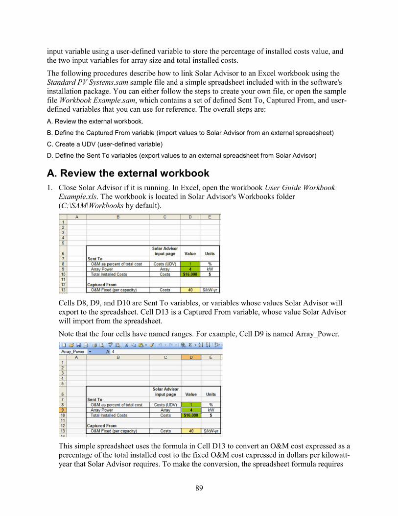
input variable using a user-defined variable to store the percentage of installed costs value, and the two input variables for array size and total installed costs.

The following procedures describe how to link Solar Advisor to an Excel workbook using the Standard PV Systems.sam sample file and a simple spreadsheet included with in the software's installation package. You can either follow the steps to create your own file, or open the sample file Workbook Example.sam, which contains a set of defined Sent To, Captured From, and user-defined variables that you can use for reference. The overall steps are: A. Review the external workbook.

B. Define the Captured From variable (import values to Solar Advisor from an external spreadsheet)

C. Create a UDV (user-defined variable)

D. Define the Sent To variables (export values to an external spreadsheet from Solar Advisor)

A. Review the external workbook 1. Close Solar Advisor if it is running. In Excel, open the workbook User Guide Workbook

Example.xls. The workbook is located in Solar Advisor's Workbooks folder (C:\SAM\Workbooks by default).

Cells D8, D9, and D10 are Sent To variables, or variables whose values Solar Advisor will export to the spreadsheet. Cell D13 is a Captured From variable, whose value Solar Advisor will import from the spreadsheet.

Note that the four cells have named ranges. For example, Cell D9 is named Array_Power.

This simple spreadsheet uses the formula in Cell D13 to convert an O&M cost expressed as a percentage of the total installed cost to the fixed O&M cost expressed in dollars per kilowatt-year that Solar Advisor requires. To make the conversion, the spreadsheet formula requires

89

the O&M as a percentage of total cost, which is not an input variable in Solar Advisor. In the next steps, we will create a user-defined variable to store that value. The other two values required by the formula, array power and total installed costs, are Solar Advisor input variables.

2. Close Microsoft Excel. If you made any changes to the workbook, do not save the changes.

B. Define the Captured From variable Use a Captured From variable to import values to Solar Advisor from an external spreadsheet.

1. Open Standard PV Systems.sam. The files is located in Solar Advisor's sample file folder (C:\SAM\Samples by default).

2. On the Residential case's Costs page, right-click the input box for the Fixed(per capacity) variable. (The value in the screenshots below may be different from the value on your screen.)

3. Solar Advisor displays the Input Type window.

90

4. In the Input Type window, click Captured From, under Workbook, click , and double-click the workbook name User Guide Workbook Example.xls.

5. In the Input Type window, click the Named Range arrow and select Fixed_per_Capacity. Note that all named ranges in the workbook appear in the Named Range list.

6. Solar Advisor displays the value from the workbook in the box with a yellow background.

If want to view the workbook, you can click the button next to named range. If you do so, do not change any values or formulas in the workbook while Solar Advisor is open. If you want to edit a connected workbook, close Solar Advisor, and then open the workbook in Excel.

7. Click OK to return to the main window. Solar Advisor displays the Captured From variable with a yellow background to indicate that it is connected to an external workbook.

C. Create a UDV 1. On the Residential case's Costs page, click Add UDV.

2. In UDV window, under User Defined Variable, for Label, type "OM per Installed Cost", and for Units, type "%". Use only letters, spaces, hyphens, or underscores for variable names. (Avoid using the ampersand character, &.)

3. Under Sent To, select the workbook User Guide Workbook Example.xls, and under Named Range select Percent_Installed_Costs.

91

4. Click OK to return to the Costs page. Solar Advisor displays the user-defined variable at the

bottom of the page.

Tip. To edit the properties of the UDV, right-click the variable.

D. Define the Sent To variables Define Sent To variables to export values to an external spreadsheet from Solar Advisor.

1. On the Residential case's Array page, right-click Array Power to open the Sent To window.

2. Under Sent To, select the workbook User Guide Workbook Example.xls, and select the Named Range Array_Power.

3. Click OK to return to the Array page.

92

4. Use the same procedure on the Costs page to define Total Installed Costs as a Sent To variable for the workbook's Installed_Costs named range.

Tip. You can send the value of a single Solar Advisor input variable to more than one cell in either a single workbook or different workbooks. To send the value to additional cells, add a row for each cell to the table in the Sent To window and select the workbook name and named range.

5. Click OK to return to the main window.

6. On the View menu, click SentTo variables and CapturedFrom variables to display lists of the variables that are connected to the workbook.

You can double click a variable name in either the SentTo or CapturedFrom window to open the page that contains the variable.

You have now defined a set of variables that interact with the Excel workbook. When you change a variable's value in Solar Advisor that affects one of the Sent To variable's values or change the value of the UDV and click the Run button, Solar Advisor recalculates the value of the O&M variable Fixed (per capacity) and displays it on the Costs page.

7. On the Costs page, type "2" for the UDV OM per Installed Cost. Solar Advisor uses the spreadsheet to recalculate the value of Fixed (per capacity). You may need to switch to a different page, for example the BOS page, and then switch back to the cost page to see the recalculated value.

93

Managing UDVs, Sent To and Captured From Variables • You can edit a UDV, Sent To or Captured From variable by right-clicking the variable's box.

• To delete a UDV, right-click the UDV's box to open the UDV window, and click Delete UDV in the bottom right corner of the window.

• To disable a Captured From variable and preserve the connection between Solar Advisor and

the external workbook, right-click the variable name on a Solar Advisor input page, and in the Input Type window, click User-Specified.

• To completely delete the connection between a Captured From variable and a workbook,

right-click the variable name on a Solar Advisor input page, and in the Input Type window, select the workbook name and press the Delete key. Be sure to select the entire workbook name and path.

94

• To delete the connection between a Sent To variable and a workbook, right-click the variable

name on a Solar Advisor input page, and in the Sent To window, select the row for the connection you want to delete and press the Delete key. Make sure both the complete workbook name and named range are highlighted.

Appendix 1: Levelized cost of energy (LCOE) Levelized cost of energy (LCOE) is an economic measure that is useful for comparing and ranking technology options because it is a cost that accounts for the purchase, financing, tax, and operation of a power system over its lifetime. Analysts can use the LCOE to evaluate different energy efficiency and renewable energy projects and to compare them to conventional fossil fuel projects.

Solar Advisor calculates the LCOE for residential, commercial, and utility projects. The residential and commercial projects are for systems connected to the grid on the customer's side of the meter. Utility projects are for systems connected on the utility side of the meter.

The LCOE accounts for project costs associated with generating electricity, but not for revenue earned from electricity sales. The LCOE is an attractive metric for comparing central and distributed generation projects. As a $/kWh value, the LCOE is comparable to the cost of conventional generation for utility-scale projects, and to the cost of electricity purchases for commercial and residential projects. The LCOE is also useful for comparing solar projects to other renewable and non-renewable projects because it accounts for both project capital requirements (typically higher for renewable and lower for non-renewable projects) and project

95

fuel and other operating costs (typically lower for renewable and higher for non-renewable projects).

The LCOE calculation depends on whether a project recovers costs through savings in electricity purchases, or through sales of electricity. Residential and commercial projects typically recover costs through electricity savings, while utility projects recover costs through electricity sales.

Residential and commercial LCOE The LCOE for residential or commercial projects (except commercial projects with third party ownership financing) is the cost per unit of energy, that, when multiplied by the total energy produced and discounted to a base analysis year, is equivalent to the present value of the total life-cycle cost of the project:

∑∑== +

=+

× N

nn

nN

nn

n

dC

dLCOEQ

01 )1()1(

Where Qn is the energy produced by the project in year n, N is the project life in years, Cn is the project net cash flow in year n, and d is the discount rate. Solar Advisor calculates Qn based on the solar radiation and other climate data, and the parameters of the software's system performance models. The summation in the left hand term begins at n = 1, which is the first year that the project produces energy. The right hand summation starts at n = 0 to include first costs in the calculation, i.e., C0 is equivalent to the project's capital costs.

Solving for LCOE gives:

∑

∑

=

=

+

+=

N

nn

n

N

nn

n

dQ

dC

LCOE

1

0

)1(

)1(

The numerator is the total life cycle cost, and the denominator is can be thought of as the total discounted annual energy output.

Utility LCOE For utility projects and commercial projects with third party ownership financing, the LCOE is the cost per unit of energy, that, when multiplied by the total energy produced over the project life and discounted to the base analysis year, is equivalent to the present value of the project required revenues over the project life given a set of financing constraints defined on the Financials page.

The required revenue is a target, and is different from the actual revenue earned by the project.

96

∑∑== +

=+

× N

nn

N

nn

n

ddLCOEQ

1

nrequired,

1 )1(R

)1(

Where Qn is the energy produced by the project in year n, calculated based on solar radiation and other climate data and the parameters of the software's system performance models. N is the project life in years, Rrequired,n is the required project revenue due to electricity sales in year n, and d is the discount rate. The summation in the left hand term begins at n = 1, which is the first year that the project produces energy. The right hand summation also starts at n = 1, the first year that the project earns revenue.

Solving for LCOE:

∑

∑

=

=

+

+=

N

nn

n

N

nn

dQ

dLCOE

1

1

nrequired,

)1(

)1(R

Real and nominal LCOE Solar Advisor calculates both the real LCOE and the nominal LCOE. The form of the discount rate in the denominator's total energy output term determines the form of the LCOE. For the real LCOE, the real discount rate appears in the total energy output term:

∑

∑∑

=

==

+

++= N

nn

real

n

N

nn

N

nn

n

dQ

ddC

1

1

nrequired,

0

)1(

)1(R

or )1(LCOE real

Similarly, for the nominal LCOE, the nominal discount rate appears in the total energy output term:

∑

∑∑

=

==

+

++=

N

nn

n

N

nn

N

nn

n

dQ

ddC

1 nominal

1

nrequired,

0

)1(

)1(R

or )1(LCOE nominal

The form of the discount rate in the cost or revenue term of the numerator does not affect its value, as long as the same form is used for the calculation of all cash flows or revenue streams. Solar Advisor uses nominal discount rates for the calculation of cash flows and revenue streams.

97

The real discount rate and nominal discount rate are related by Equation 7, where dnominal is the nominal discount rate, dreal is the real discount rate, and e is the inflation rate:

dnominal = (1 + dreal)(1 + e) - 1

Appendix 2: Cash Flow Solar Advisor reports the cash flow as a stream of annualized costs in two formats: the net annual cash flow in the Cashflow graph on the Results Summary page, and cash inflow and outflow details on the cash flow tab of the results spreadsheet. A positive cash flow for a given year indicates net earnings (inflow) in that year, and a negative net cash flow indicates net losses (outflow) for that year.

This section describes the cash flow spreadsheet. The primary cash flow streams in the spreadsheet are displayed in the following rows:

• After-tax net equity cash and cost flows

• State and federal taxes

• Total operating expenses

• Total debt payment

• Project income from revenues or offset payments

Note. You can learn more about the cash flow calculations by exploring the Excel formulas in the financial spreadsheets posted on the Solar Advisor website: https://www.nrel.gov/analysis/sam/download.html.

After tax net equity cash and cost flows

All capital costs are accounted for in year zero of the cash flow. The total capital cost is equal to the equity portion of the total capital investment and shown in the Equity Funds row of the spreadsheet. For cash projects, Equity Funds is equal to Total Installed Costs on the Costs page. For projects financed by a loan or mortgage, Equity Funds is Total Installed Costs on the Costs page minus Debt Funds. Debt Funds is Loan (Debt) Percent from the Financials page multiplied by the total installed costs.

Year one is the first year of operation. For residential and commercial systems, the cash flow for year one and subsequent years is given by:

98

After Tax Net Equity Cash Flow = After Tax Net Equity Cost Flow +

Residential: Offset Payments Commercial: Offset Payments - Offset Payments x Effective Tax Rate Utility: Operating Income

The effective tax rate is a single rate that includes both the state tax rate and federal tax rate.

The cost flow for all project types in year one and subsequent years is:

After Tax Net Equity Cost Flow = State Tax Savings (Liability) + Federal Tax Savings (Liability) + PBI Incentives - Total Operating Expenses - Total Debt Payment

Note. Utility projects with independent power producer (IPP) financing do not show the cost flow row in the spreadsheet. Utility projects with investor-owned utility (IOU) financing show a required revenue stream in the cash flow spreadsheet instead of the cost and cash flows.

State and federal taxes

All projects except investor-owned utility (IOU) projects pay state and federal taxes on the total taxable income for each year when the state and federal annual tax rates on the Financials page are non-zero. Federal and state tax cash flows are displayed in two separate sections of the cash flow spreadsheet, under the rows labeled Tax Effect on Equity (Federal) and Tax Effect on

99

Equity (State). The tax amount for each year appears in the Tax Savings (Liability) row under each section.

For both federal and state taxes, a positive value of Tax Savings (Liability) indicates a tax savings or cash inflow. A negative value indicates a tax liability or cash outflow. It is calculated as follows:

Tax Savings (Liability) [State or Federal] = Income Taxes [State or Federal] - Production Tax Credit - Investment Tax Credit

• The production tax credit (PTC), if it applies, is calculated for each year by multiplying the tax credit percentage shown on the Incentives page by the value shown in the Electric Output (kWh) row of the cash flow spreadsheet.

• When an investment tax credit (ITC) applies, it is subtracted only in year one of the project; it is not subtracted in year two and subsequent years. The ITC is either equal to the fixed amount on the Incentives page, or calculated by multiplying the ITC percentage on the Incentives page by the total installed costs on the Costs page.

A note about incentives. Some incentives have caps that limit their maximum value, while others have escalation rates that increase their value from year to year. Others have term limits that end payments after a given number of years. In some cases the incentive income is taxable at the federal or state level, and in other cases it is not. Finally, investment and capacity based incentives may or may not reduce the basis on which the investment tax credit (ITC) is calculated. All of these factors are defined on the Incentives page.

Federal and state income taxes are calculated as follows:

Income Taxes [State or Federal] = Total Taxable Income x Tax Rate [State or Federal]

• The total taxable income is the project income less deductible expenses. Deductible expenses include operating expenses, depreciation, interest payments, and sales tax payments. In year one, projects may pay sales tax on the total capital costs incurred in year zero. The sales tax rate is on the Financials page.

• For residential, commercial, and utility projects, income includes receipts from incentive payments. For utility projects, income also includes revenues from electricity sales.

• Cash inflow from state tax (state tax savings) is included in the federal taxable income. State tax outflow (liability) is deducted from the federal taxable income.

100

Total operating expenses

The total operating expenses include operation and maintenance costs, and insurance and property tax payments.

Total Operating Expenses = Fixed (Annual) O&M Expense + Fixed O&M Expense + Variable O&M Expense + Insurance + Property Taxes

The operation and maintenance (O&M) costs are defined on the Costs page, and escalated in each year after year one using both the escalation rate for each O&M category on the Costs page and the inflation rate value on the Financials page. The insurance and property tax rates are also both on the Financials page, and apply to the total installed cost value on the Costs page.

Total debt payment

For projects financed by a loan or mortgage, the total debt payment is the sum of interest and principal payments:

Total Debt Payment = Debt Interest Payment + Debt Payment

Payments are calculated annually. The annual interest payment is the product of Rate and Loan (Debt) Fraction on the Financials page and Total Installed Costs on the Costs page. Debt Payment is the principal payment, and is a function of the Rate, Term, and Loan (Debt) Fraction on the Financials page.

101

Project income (revenue and offset payments)

Residential and commercial projects may receive net-metering offset payments for electricity generated by the project. Commercial projects also pay federal and state income tax on the payments as shown in the explanation for after tax net equity cash flow above. The electricity purchase price is equal to Flat Rate on the Utility Rates page.

Offset Payments = Electric Output x Electricity Purchase Price

For utility projects, the operating income is determined in each year by the annual output and the electricity sales price. For residential and commercial projects, the sales price is equal to Flat Rate on the Utility Rates page. For utility projects, Solar Advisor calculates the year one sales price to meet the financing constraints on the Financials page, and calculates the sales price in year two and subsequent years based on the first year sales price and the PPA escalation rate on the Financials page.

Revenues = Electric Output x Electricity Sales Price

Operating Income = Revenues - Total Operating Expenses

Appendix 3: Equations for Calculated Values Solar Advisor displays some variables throughout the user interface with blue backgrounds, indicating that the values are calculated and cannot be edited. This chapter describes the calculations behind these variables. The calculations described in this chapter are different from the performance simulation calculations, which are described in a separate reference manual, available for download on the Solar Advisor website: https://www.nrel.gov/analysis/sam.

102

Financials The two calculated values on the Financials page are the loan amount and the weighted average cost of capital.

Loan Amount The loan amount is the amount borrowed by the project, and is a percentage of the total installed costs from the Costs page.

Weighted Average Cost of Capital

The weighted average cost of capital (WACC) is defined as the minimum return that the project must earn to cover financing costs.

The effective tax rate is a single value that accounts for both state and federal income taxes, calculated from the state tax rate and federal tax rate.

For residential and commercial projects, the return on equity is equal to the discount rate, which is an input on the Financials page:

For utility projects, the return on equity is the required internal rate of return, also an input on the Financials page:

103

Equation Variable Solar AdvisorLoanAmount Amount

CTotalInstalled Total Installed Costs on the Costs page

FDebtFraction Loan (Debt) Fraction

FLoanRate Rate DiscountRate Real Discount Rate RequiredIRR Required Internal Rate of Return (IRR)

PV Array Layout The calculated values on the array page for photovoltaic systems are based on values of variables on the Array page, and on variables on the Module page and Inverter page.

Total Modules Total modules is the number of modules in the array.

Array Power The array power is the maximum DC power output of the array.

Voltage ratings: Voc (string), Vmp (string), and Vnom (dc-inverter) The voltage ratings are displayed for reference to help you choose a number of inverters based on the size of each string of modules.

The open circuit voltage (Voc) and maximum power point voltage (Vmp) of each string of modules and depends on the module ratings and the number of modules per string. The voltage ratings do not apply to the single-point efficiency module performance model because the model does not include voltage ratings.

104

The inverter nominal DC voltage (Vnom) is for a single inverter, and does not apply to the single-point efficiency inverter performance model.

Inverter Power The inverter power is the total DC power rating of all inverters for reference when sizing the array.

105

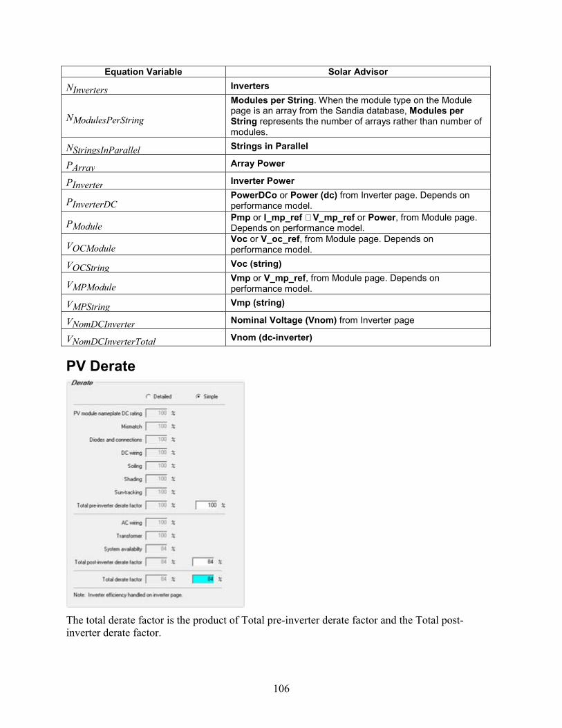
Equation Variable Solar Advisor

NInverters Inverters

NModulesPerString

Modules per String. When the module type on the Module page is an array from the Sandia database, Modules per String represents the number of arrays rather than number of modules.

NStringsInParallel Strings in Parallel

PArray Array Power

PInverter Inverter Power

PInverterDC PowerDCo or Power (dc) from Inverter page. Depends on performance model.

PModule Pmp or I_mp_ref V_mp_ref or Power, from Module page. Depends on performance model.

VOCModule Voc or V_oc_ref, from Module page. Depends on performance model.

VOCString Voc (string)

VMPModule Vmp or V_mp_ref, from Module page. Depends on performance model.

VMPString Vmp (string)

VNomDCInverter Nominal Voltage (Vnom) from Inverter page

VNomDCInverterTotal Vnom (dc-inverter)

PV Derate

The total derate factor is the product of Total pre-inverter derate factor and the Total post-inverter derate factor.

106

In Detailed mode, the Total pre-inverter derate factor is the product of all of the pre-inverter derate factors, and the Total post-inverter derate factor is the product of AC wiring, Transformer, and System availability derate factors.

PV Module The values that appear on the Module page for flat-plate photovoltaic modules depend on the performance model. For the Sandia PV Array Performance Model and the CEC Performance Model, the values with blue backgrounds are stored in database files in the SAM\Data\KingDatabase folder and SAM\Data\Modules folder, respectively.

For the Single Point Efficiency Model for both flat-plate and concentrating photovoltaic modules, Power is a calculated value described below.

Power On the Module page for photovoltaic systems using the single-point efficiency performance model, Power is the maximum DC output of the module.

The module's maximum power is the product of the module efficiency, irradiance at standard test conditions (1,000 W/m2), and the module area.

For flat-plate modules, Temperature Coefficient (Pmax) and Module Structure are used by the simulation engine to calculate the module's hourly output.

Equation Variable Solar Advisor

PModule Power

ηModule Efficiency

AModule Area

PV Inverter The values that appear on the Inverter page for photovoltaic systems modules depend on the performance model. For the Sandia Performance Model for Grid-Connected PV Inverters, the values with blue backgrounds are stored in database files in the SAM\Data\Inverter folder.

107

For the Single Point Efficiency Model Power (dc) is a calculated value described below.

Equation Variable Solar Advisor

PInverterAC Power (ac)

PInverterDC Power (dc)

ηInverter Efficiency

CSP Solar Field Solar Field Area, Solar Multiple, and Exact Area

When the Layout option is Solar Multiple, Solar Advisor calculates the solar field area based on the value you enter for the solar multiple:

When the Layout option is Solar Field Area, Solar Advisor calculates the solar multiple based on the value you enter for the solar field area:

The exact area is the solar field area for a solar multiple of one calculated as follows:

108

The values used for these equations are displayed under Solar Multiple Reference Conditions and Values From Other Pages, except for the five FET factors, which are on the Power Block page.

Note. Direct Normal Radiation does not represent weather conditions at the site, but is the reference radiation value used to calculate the solar field area when the solar multiple is one.

Equation Variable Solar Advisor

AExactArea Exact Area

ASolarField Solar Field Area

ASolarFieldCalculated Solar Field Area (calculated)

FET0...FET4 Turb. Part Load Elec to Therm from the Power Block page

FSolarMultiple Solar Multiple

FSolarMultipleCalculated Solar Multiple (calculated)

ηOpticalEfficiency Optical Efficiency from the SCA / HCE page

QDesignTurbineThermalInput Design Turbine Thermal Input from the Power Block page

QDirectNormalRadiation Direct Normal Radiation

QHCEThermalLosses HCE Thermal Losses from the SCA / HCE page

QSolarFieldPipingHeatLosses Solar Field Piping Heat Losses

Exact Number of SCAs

Equation Variable Solar Advisor

AApertureAreaPerSCA Aperture Area per SCA, equivalent to SCA Aperature Area on SCA / HCE page

AExactArea Exact Area

NExactNumberOfSCAs Exact Number of SCAs

Solar Field Piping Heat Losses The solar field piping heat losses are calculated using parameters of the heat transfer fluid and the reference ambient temperature:

109

Equation Variable Solar Advisor

FPHL1 ... FPHL3 Piping Heat Loss Temp Coeff 1 through 3

QSFPipeHLDesign Solar Field Piping Heat Losses @ Design T

QSolarFieldPipeHeatLosses Solar Field Piping Heat Losses

TAmbient Ambient Temperature

TSFinDesign Solar Field Inlet Temperature

TSFoutDesign SolarField Outlet Temperature

CSP SCA / HCE HCE Optical Efficiency

Solar Advisor displays a value for Optical Efficiency (HCE) for each of the four Receiver types. The value is calculated for each receiver type by multiplying the four Optical Parameters values together:

• Bellows Shadowing

• Envelope Transmissivity

• Absorber Absorption

• Unaccounted And then multiplying the result by the product of the six SCA factors:

• Tracking Error and Twist

• Geometric Accuracy

• Mirror Reflectivity

• Mirror Cleanliness Field (field avg)

• Dust on Envelope (field avg)

110

• Concentrator Factor The weighted optical efficiency, Optical Efficiency (Weighted), is the sum of the products of each receiver type's Optical Efficiency (HCE) and Percent of Field.

HCE Heat Losses

The heat loss for each HCE type depends on the value of the six heat loss coefficients and heat loss factor for each HCE type, and on the solar field heat transfer fluid temperature design parameters:

Where:

The total, or weighted HCE losses are expressed both in terms of the SCA aperture length:

And the SCA aperture area:

111

Equation Variable Solar Advisor

FA0 ... FA6 A0 Heat Loss Coefficient through A6 Heat Loss Coefficient

FHeatLossFactor Heat Loss Factor

QHCELosses Receiver Heat Losses (W/m)

QHCELossesWeightedW/m Thermal Losses (Weighted W/m)

QHCELossesWeightedW/m^2 Thermal Losses (Weighted W/m2)

TAmb Ambient Temperature from the Solar Field page

TSFin Solar Field Inlet Temperature from the Solar Field page

TSFout Solar Field Outlet Temperature from the Solar Field page

νWind Wind Velocity from the Solar Field page

CSP Power Block Design Turbine Thermal Input

Equation Variable Solar Advisor

ηDesignTurbineGross Design Turbine Gross Efficiency

QDesignTurbineGross Design Turbine Gross Output

QDesignTurbineThermalInput Design Turbine Thermal Input

CSP Storage Maximum Energy Storage

112

Heat Exchanger Duty

The heat exchanger duty depends on the value of the solar multiple. When the solar multiple is greater than one:

When the solar multiple is equal to or less than one:

Maximum Power To and From Storage

The maximum power to and from storage depends on whether the TES includes a heat exchanger. When the TES fluid is different from the solar field fluid, the TES includes a heat exchanger. When the fluids are the same, there is no heat exchanger.

For a TES with heat exchanger (TES fluid and solar field fluid are different):

For a TES with no heat exchanger (TES fluid and solar field fluid are the same):

113

Equation Variable Solar Advisor

FHeatExchangerDuty Heat Exchanger Duty

FSolarMultiple Solar Multiple from Solar Field page

FTESAdjustEfficiency Turbine TES Adj. - Efficiency

FTESAdjustOutput Turbine TES Adjustment - Gross Output

FTurbineMaximumOverDesign Max Over Design Operation from Power Block page

NHoursOfStorage Equiv. Full Load Hours of TES

PMaximumFromStorage Maximum Power From Storage

PMaximumToStorage Maximum Power To Storage

QDesignTurbineInput Design Turbine Thermal Input from Power Block page

QMaximumStorage Maximum Energy Storage

CSP Parasitics

For each source of parasitic losses, the design point parasitic loss value is the product of either Factor, PF, and Solar Field Area; or the product of Factor, PF, and Gross Turbine Output, except for the antifreeze pumping losses and night circulation pumping losses, which are a function of Factor and Solar Field HTF Pump:

114

Source of Parasitic Loss Equation Collector Drives and Electronics Factor x PF x Solar Field Area Solar Field HTF Pump Factor x PF x Solar Field Area Thermal Energy Storage Pumps Factor x PF x Gross Turbine Output Antifreeze Pumping Factor x Solar Field HTF Pump losses Night Circulation Pumping Factor x Solar Field HTF Pump losses Power Block Fixed Factor x Gross Turbine Output Balance of Plant Factor x PF x Gross Turbine Output Heater/Boiler Factor x PF x Gross Turbine Output Cooling Towers Factor x PF x Gross Turbine Output

Total Design Point Parasitics is the sum of the following losses (it does not include antifreeze pumping or night circulation pumping losses):

• Collector Drives and Electronics

• Solar Field HTF Pump

• Night Circulation Pumping

• Power Block Fixed

• Balance of Plant

• Heater/Boiler

• Cooling Towers

Effective tax rate The effective tax rate is a single number that includes both the federal income tax rate and state income tax rate. Solar Advisor uses the effective tax rate for several calculations requiring a total income tax value.

The effective tax rate calculation is:

EffectiveTaxRate = FederalTaxRate × (1- StateTaxRate) + StateTaxRate

The federal tax rate and state tax rate are input variables on the Financials page.

115

References Weather data Typical Meteorological Year (TMY2 and TMY3) data and documentation is available on the Solar Radiation Resource Information website. http://rredc.nrel.gov/solar/old_data/nsrdb

Information about EnergyPlus weather data is available on the EnergyPlus website. http://www.eere.energy.gov/buildings/energyplus/cfm/weather_data.cfm

Project economics financing Short et al, 1995. Manual for the Economic Evaluation of Energy Efficiency and Renewable Energy Technologies. National Renewable Energy Laboratory. NREL/TP-462-5173. http://www.nrel.gov/docs/legosti/old/5173.pdf

Wiser, 1997. "Renewable energy finance and project ownership", Energy Policy Vol 25 No 1 pp 15-27.

Wiser et al, 1997. Financing Investments in Renewable Energy: The Role of Policy Design and Restructuring. Ernest Orlando Lawrence Berkeley National Laboratory. http://eetd.lbl.gov/ea/EMS/reports/39826.pdf

Performance models King et al, 2004. Photovoltaic Array Performance Model. Sandia National Laboratories. SAND2004-3535. http://www.prod.sandia.gov/cgi-bin/techlib/access-control.pl/2004/043535.pdf

King et al, 2007. Performance Model for Grid-Connected Photovoltaic Inverters. Sandia National Laboratories. SAND2007-5036. http://www.prod.sandia.gov/cgi-bin/techlib/access-control.pl/2007/075036.pdf

California Energy Commission, New Solar Homes Partnership Calculator: CECPV Calculator. The CEC calculator uses the same module performance model as Solar Advisor's CEC performance model; documentation included with the CECPV Calculator explains details of the model. http://www.gosolarcalifornia.ca.gov/nshpcalculator

Arizona State Photovoltaic Testing Laboratory. http://www.poly.asu.edu/ptl

CSP technology NREL Troughnet Parabolic Trough Solar Power Network. http://www.nrel.gov/csp/troughnet

Moens et al, 2005. Advanced Heat Transfer and Thermal Storage Fluids, National Renewable Energy Laboratory. NREL/CP-510-37083. http://www.nrel.gov/docs/fy05osti/37083.pdf

116

Price et al, 2006. Field Survey of Parabolic Trough Receiver Thermal Performance, National Renewable Energy Laboratory NREL/CP-550-39459. http://www.nrel.gov/docs/fy06osti/39459.pdf

For more detailed information, see NREL, 2000. Survey of Thermal Storage for Parabolic Trough Power Plants. National Renewable Energy Laboratory. NREL/SR-550-27925. http://www.nrel.gov/csp/troughnet/pdfs/27925.pdf

TRNSYS and Excelergy Klein et al, 2004. TRNSYS 16, A Transient Simulation Program. Solar Energy Laboratory, University of Wisconsin, Madison, Wisconsin, WI. http://sel.me.wisc.edu/trnsys/

NREL has used Excelergy in analysis for the Department of Energy, Sargent and Lundy, and the Southwest Concentrating Solar Power 1000 MW Initiative. See http://www.nrel.gov/csp/modeling_analysis.html#systems

Useful web sites Sandia National Laboratories: Photovoltaic Systems Research & Development, http://photovoltaics.sandia.gov; Concentrating Solar Power and SunLab, http://energylan.sandia.gov/sunlab.

National Renewable Energy Laboratory: Energy Analysis, http://www.nrel.gov/analysis; National Center for Photovoltaics, http://www.nrel.gov/pv;Concentrating Solar Power Research, http://www.nrel.gov/csp.

Go Solar California: http://www.gosolarcalifornia.ca.gov.

U.S. Department of Energy Solar Energy Technologies Program: http://www1.eere.energy.gov/solar.

117

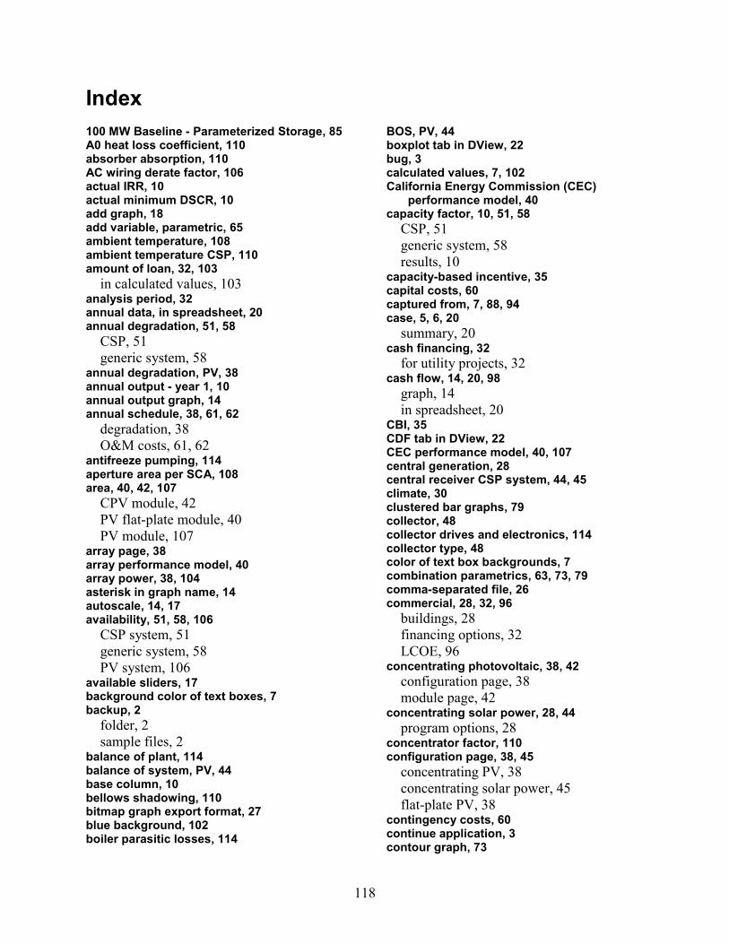
Index 100 MW Baseline - Parameterized Storage, 85 A0 heat loss coefficient, 110 absorber absorption, 110 AC wiring derate factor, 106 actual IRR, 10 actual minimum DSCR, 10 add graph, 18 add variable, parametric, 65 ambient temperature, 108 ambient temperature CSP, 110 amount of loan, 32, 103

in calculated values, 103 analysis period, 32 annual data, in spreadsheet, 20 annual degradation, 51, 58

CSP, 51 generic system, 58

annual degradation, PV, 38 annual output - year 1, 10 annual output graph, 14 annual schedule, 38, 61, 62

degradation, 38 O&M costs, 61, 62

antifreeze pumping, 114 aperture area per SCA, 108 area, 40, 42, 107

CPV module, 42 PV flat-plate module, 40 PV module, 107

array page, 38 array performance model, 40 array power, 38, 104 asterisk in graph name, 14 autoscale, 14, 17 availability, 51, 58, 106

CSP system, 51 generic system, 58 PV system, 106

available sliders, 17 background color of text boxes, 7 backup, 2

folder, 2 sample files, 2

balance of plant, 114 balance of system, PV, 44 base column, 10 bellows shadowing, 110 bitmap graph export format, 27 blue background, 102 boiler parasitic losses, 114

BOS, PV, 44 boxplot tab in DView, 22 bug, 3 calculated values, 7, 102 California Energy Commission (CEC)

performance model, 40 capacity factor, 10, 51, 58

CSP, 51 generic system, 58 results, 10

capacity-based incentive, 35 capital costs, 60 captured from, 7, 88, 94 case, 5, 6, 20

summary, 20 cash financing, 32

for utility projects, 32 cash flow, 14, 20, 98

graph, 14 in spreadsheet, 20

CBI, 35 CDF tab in DView, 22 CEC performance model, 40, 107 central generation, 28 central receiver CSP system, 44, 45 climate, 30 clustered bar graphs, 79 collector, 48 collector drives and electronics, 114 collector type, 48 color of text box backgrounds, 7 combination parametrics, 63, 73, 79 comma-separated file, 26 commercial, 28, 32, 96

buildings, 28 financing options, 32 LCOE, 96

concentrating photovoltaic, 38, 42 configuration page, 38 module page, 42

concentrating solar power, 28, 44 program options, 28

concentrator factor, 110 configuration page, 38, 45

concentrating PV, 38 concentrating solar power, 45 flat-plate PV, 38

contingency costs, 60 continue application, 3 contour graph, 73

118

conventional, 44, 58 fossil fuel plant, 58 power cycle in CSP, 44

converting data into TMY2 format, 30 cooling tower, 51, 58, 114

correction, 51 operation mode, 58 parasitic losses, 114

copy, 27 bitmap, 27 metafile,, 27

cost, 14, 60, 61 capital, 60 data, 60 O&M, 61 stacked bar graph, 14

CPV, 38, 42 configuration page, 38

CSP, 44 system components, 44

csv, 26 current, 104

PV maximum power point, 104 daily tab, DView, 22 database of available module coefficients, 40 DC tab in DView, 22 DC voltage, 104 debt fraction, 32 debt payment, in cash flow, 101 debt service coverage ration, 32 define parametric window, 63, 65 degradation, 38, 51, 58

CSP, 51 generic system, 58 PV, 38

delete, 5, 18 case, 5 graph, 18

Department of Energy, 1 depreciation, 32 derate, 38, 58, 106

generic system, 58 PV, 38 PV calculated values, 106

design point parasitic loss, 114 design turbine parameters, 51, 54, 108, 112

in solar field page equations, 108 in storage page equations, 112 on power block page, 51 on storage page, 54

detailed derate factors, 106

detailed PV derate mode, 38 direct capital costs, 60 direct CSP storage, 54 direct normal radiation, 45, 108

reference, 45 direct normal radiatioon, 42

for CPV model, 42 discount rate, 95, 103 dish Stirling CSP system, 44, 45 DMap tab, DView, 22 download software, 2 dry cooling, CSP, 51 dry cooling, CSP sample file, 44 drybulb basis, 51 DSCR, 32 duplicate case, 5 dust on envelope, 110 duty cycle of heat exchanger, 112 DView, 24, 27

exporting graph images, 27 waterfall graph, 24

DView data viewer, 22 edit combo, 73 edit graph, 18 edit linkage, 70 edit values, parametric, 65 effective tax rate, 103, 115 efficiency, 40, 42, 43, 107, 110, 112

CPV module, 42 CSP turbine, 112 flat-plate PV module, 40 inverter, 43, 107 optical HCE, 110 PV module, 107

electric losses, 114 CSP, 114

electricity sales and savings, 95 EnergyPlus weather data format, 30 engineer procure construct costs, 60 envelope transmissivity, 110 environment, 29 EPW weather data, 30 equivalent full load hours of TES, 54, 112 error message, 3 exact area, 108 exact number of SCAs, 108 Excel, 20, 88

inputs and results, 20 link to inputs, 88

Excelergy software, 44 exchanger duty, 112 export, 26, 27

data from graphs and tables, 26

119

graph image, 27 factor, 114 federal tax, 32, 103 field background color, 7 file formats, 5 file size, 5 financials, 32, 103

calculated values, 103 financing, 32 first year PPA, 10 five-parameter PV model, 40 fixed O&M costs, 61 flat rate, 32 flat-plate photovoltaic modules, 38, 40

configuration page, 38 module page, 40

fluid for CSP storage, 112 fossil fill fraction, 54 fossil fuel, 28, 44, 58

backup for CSP systems, 44 system type, 28 system type, 58

Fresnel, 45 fuel cost for generic system, 58 generic system type, 28, 58

in program options, 28 geometric accuracy of HCE, 110 graph, 14, 17, 18, 26, 27

autoscale, 14, 17 descriptions, 14 export data, 26 export image, 27 legend, 14 name, 18 scale, 17 size, 14 sliders, 17 type, 18

graph info window, 18 grassy ground reflectance, 38 gross design turbine parameters, 51, 112,

114 in parasitic loss calculations, 114 in power block page equations, 112 in storage page equations, 112

ground reflectance, 38 HCE, 44, 108, 110

heat loss, 110 optical efficiency, 110 thermal losses, 108

heat collection element, 44, 48

heat exchanger, 51, 112 fouling and annual degradation, 51

heat loss HCE, 110 heat transfer fluid, 44, 108, 110, 112

in CSP storage calculated values, 112 temperature, 108

heater parasitic losses, 114 heating and light, 1 help, 2 hourly data, 20, 22

in DView, 22 in spreadhseet, 20

HTF, 44, 112 in CSP storage calculated values, 112

html export graph data to, 26 IBI, 35 import case, 5 incentives, 35 independent parametric, 63, 65 independent power producer, 32 indirect capital costs, 60 indirect CSP storage, 54 inflation rate, 32 initial thermal storage, 54 inlet temperature, 110 inputs spreadsheet, 20 install software, 2 insurance, 32 internal rate of return, 32, 103 inverter, 38, 104, 106, 107

calculated values, 107 capacity, 38 derate calculated values, 106 nominal DC voltage, 104 power, 38, 104, 107

inverter page, 43 investment tax credit, 35 investment-based incentive, 35 investor-owned utility, 32 IOU, 32 IPP, 32 IRR, 32, 103 ITC, 35 kWh / kW - year 1, 10 land costs, 60 layout PV array, 38, 45, 108 LCOE, 10, 14, 95, 96, 97

commercial, 96 graph, 14 in metric summary table, 10 nominal, 97 real, 97

120

residential, 96 utility, 96

legend, 7, 14 graph, 14 text box background colors, 7

levelized cost of energy (see LCOE), 95 lifecycle cost, 95 linear Fresnel, 45 linkage parametric, 63, 70 load, 37 loan, 32, 103

in calculated values, 103 loan financing, 32 losses, 58, 106, 108, 110, 114

CSP calculated values, 110, 114 CSP parasitic, 58 CSP thermal, 108 PV, 106

MACRS depreciation, 32 main window, 6 maximum over design operation CSP, 51,

112 in storage calculated values, 112

maximum power point voltage PV, 104 maximum storage energy and power CSP,

54, 112 in storage calculations, 112

metafile graph export format, 27 Meteonorm weather data software, 30 metrics table, 10, 20

in spreadsheet, 20 on results summary page, 10

minimum cash flow, 10 minimum load, 51 minimum required DSCR, 32 minimum required IRR, 32 mirror in CSP system, 44, 110

parameters in calculated values, 110 miscellaneous costs, 60 module page, 40, 42

concentrating PV, 42 flat-plate PV, 40

module PV, 40, 104, 107 calculated values, 107 performance models, 40 ratings, 104 structure, 40, 107

module structure PV, 40, 107 monthly data, 14, 20, 22

in DView, 22 in spreadsheet, 20

in standard graphs, 14 mortgage financing, 32 name graph, 18 nameplate capacity for generic system, 58 net metering, 102 net present value, 10 new file, 4 night circulation pumping, 114 nominal LCOE, 97 nominal PV array voltages, 104 NPV, 10 number of inverters, 38, 104 number of modules per string, 104 O&M costs, 61 offset payments, 102 open circuit voltage, 104 operating expenses in cash flow, 101 operation and maintenance costs, 61, 62 optical parameters HCE, 108, 110

in calculated values, 108, 110 organic Rankine-cycle turbine, 51 orientation, 38, 45

CSP solar field, 45 PV array, 38

outlet temperature, 110 output metrics table, 10 panel PV (see module PV), 40 parabolic trough CSP system, 44 Parameter1 for graph, 18 Parameter2 for graph, 18 parametric variables, 7, 63

text box background color, 7 parasitic losses CSP, 58, 114

calculated values, 114 payments offset, 102 PBI, 35 PDF tab in DView, 22 percent of field CSP, 110 PF, 114 photovoltaic, 28, 37, 38, 40, 42

concentrating PV, 38, 42 flat-plate PV, 40 program options, 28 system overview, 37

piping heat loss temp coefficient, 108 positive cashflow requirement, 32 post-inverter derate factor, 106 power, 40, 42, 43, 104, 107

CPV module, 42 inverter, 43, 107 maximum power point PV, 104 PV array, 104 PV flat-plate module, 40

121

PV module, 107 power block CSP, 51, 112, 114

calculated values, 112 fixed parasic losses, 114

power cycle, 51 power plant availability CSP, 51 power tower CSP system, 44, 45 PPA escalation rate, 32 pre-inverter derate factor, 106 price for electricity sales, 32 production-based incentive, 35 profile tab in Dview, 22 program page, 28 project costs, 60 project summary, 20 property tax, 32 pump motor losses, 58 pumping losses, 114

CSP, 114 PV array, 38, 104, 106

calculated values, 104, 106 derate factor, 106

PV array performance model, 107 PV module (see module PV), 40 Rankine power cycle, 51 rate of loan, 32 rated turbine net capacity, 51 real discount rate, 32 real LCOE, 97 receiver, 44, 48, 110

heat loss, 110 type and condition, 48 types, 110

reference conditions CSP, 108 reference turbines, 51 referenced values, 7 remove software, 2 rename case, 5 required internal rate of return, 103 reset slider, 14, 17 residential, 28, 32, 96

buildings, 28 financing options, 32 LCOE, 96

resource data, 30 restart application, 3 results, 9, 10, 14

metrics table, 10 summary page, 14 viewing, 9

return on equity, 103 revenue, 95 run analysis button, 9

SAI (Solar America Initiative), 1 sales tax, 32, 60

as indirect cost, 60 rate, 32

SAM file format, 5 sample files, 2 Sandia, 40, 43

inverter performance model, 43 PV array performance model, 40

SCA, 44, 108, 110 aperture area, 108, 110 aperture length, 110 calculated values, 110

SCA / HCE, 48 scale graph, 14, 17 schedule variable type, 7 SCIF file format, 5 selected sliders, 17 send bug report, 3 send to excel, 14, 26 sensitivity analysis, 63 sent to, 88, 94 SETP, 1 settings, 4, 9 shadowing, 110

bellows CSP, 110 show notes, 14 simple payback, 10 simple PV derate mode, 38 single-point efficiency model, 1, 40, 42, 43,

104 concentraing PV, 42 inverter, 43 PV flat-plate, 40

slider, 10, 14, 17 column column in metrics table, 10 reset, 17 selection window, 17

slow startup, 4, 9 snowy ground reflectance, 38 Solar America Initiative, 1 solar collector assembly, 44, 48 Solar Energy Technologies Program, 1 solar field, 45

size, 45 solar field CSP, 108, 110, 112, 114

area calculated, 108 area in calculated values, 108 area in parasitic calculated values, 114 calculated values, 108 heat transfer fluid, 112

122

HTF pump in parasitic calculated values, 114

inlet temperature, 108 outlet temperature, 108 piping heat losses, 108 temperature, 110

solar field page, 45 solar heating and lighting, 1, 28 solar multiple, 45, 85, 108, 112 solar multiple calculated, 108 solar resource data, 30 specify range, 65 speed up the display speed, 9 spreadsheets, 20, 88

inputs and results, 20 linked to inputs, 88

Standard CSP Systems.sam, 44 Standard PV Systems.sam, 37 startup mode, 9 state tax, 32, 103

rate in calculated values, 103 Stirling engine, 45 storage, 44, 54, 112

CSP, 54 CSP calculated values, 112 PV, 44

storage dispatch fraction, 54 storage fluid number, 54 straight line depreciation, 32 strings, 104

modules in PV array, 104 strings in parallel, 104 support, 2 system availability, 106

PV, 106 system degradation, 38 Systems Driven Approach, 1 tabs, 5, 6, 22

for different cases, 5, 6 in DView, 22

tank heat losses, 54 tax, 32, 35, 99, 103, 115

credits, 35 effective tax rate, 115 in calculated values, 103 in cash flow, 99 property, 32

tax adjusted utility rate, 10 technical support, 2 temperature, 108, 110

ambient CSP, 110

CSP heat transfer fluid, 108 solar field, 110

temperature correction, 40, 51, 107 CSP mode, 51 PV coefficient, 40, 107

temporary folder, 20, 26 term of loan, 32 TES (see thermal energy storage system), 54 text box backgournd colors, 7 thermal energy storage system, 44, 54, 112,

114 fluid, 112 pumping parasitic losses, 114

thermal input of design turbine, 112 thermal loss CSP, 110 thermal storage dispatch controls, 54 thermocline, 54 third party ownership, 32 time of use, 32, 54

periods, 32, 54 rates, 32

time series graphs button, 22 TMY weather data, 30 total design point parasitics, 114 total installed costs, 103 total inverter derate factors, 38, 106

calculated values, 106 total lifecycle cost, 95 total modules, 38, 104 TOU (see time of use), 32 tracking, 38, 45

CSP solar field, 45 PV array, 38

tracking error and twist CSP, 110 transformer derate factor, 106 transmissivity HCE, 110 TRNSYS, 1 turbine, 51 turbine - TES Adjustment, 54 turbine output fraction, 54 turbine part load electric to thermal, 108 turbine part load thermal to electric, 51 turbine start-up, 51 turbine TES adjustments, 112 two tank storage CSP, 54 Typical Meteorological Year, 30 UDV, 88, 91, 94 UDV button, 6 unaccounted parameter of HCE, 110 undo, 9 uninstall software, 2 University of Wisconsin, 1 user assistance, 2 user defined variable, 91

123

124

user defined variables button, 6 user specified, 7 user support, 2 user-defined variable, 88, 94 utility, 32

cash financing for, 32 financing options, 32

utility LCOE, 96 utility rate, 32 variable background color, 7 variable names, 22, 24

in DView, 22 in waterfall graphs, 24

variable O&M costs, 61 version number, 1 view input type legend, 7 voltage, 104

Inverter, 104 PV array, 104

WACC, 103 waterfall graphs, 24 weather data format, 30 weighted average cost of capital, 103 weighted optical efficiency, 110 wetbulb basis, 51 wind velocity, 110 workbooks, 20, 88

inputs and results, 20 linked to inputs, 88

X Values for graphs, 18 xml export graph data to, 26 Y2 Values for graphs, 18 year-by-year, 38, 61, 62

degradation, 38 O&M costs, 61, 62

YValues for graphs, 18 ZIP file format, 5 ZValues for graphs, 18

F1146-E(12/2004)

REPORT DOCUMENTATION PAGE Form Approved OMB No. 0704-0188

The public reporting burden for this collection of information is estimated to average 1 hour per response, including the time for reviewing instructions, searching existing data sources, gathering and maintaining the data needed, and completing and reviewing the collection of information. Send comments regarding this burden estimate or any other aspect of this collection of information, including suggestions for reducing the burden, to Department of Defense, Executive Services and Communications Directorate (0704-0188). Respondents should be aware that notwithstanding any other provision of law, no person shall be subject to any penalty for failing to comply with a collection of information if it does not display a currently valid OMB control number. PLEASE DO NOT RETURN YOUR FORM TO THE ABOVE ORGANIZATION.1. REPORT DATE (DD-MM-YYYY)

August 2008 2. REPORT TYPE

Technical report 3. DATES COVERED (From - To)

4. TITLE AND SUBTITLE

Solar Advisor Model User Guide for Version 2.0 5a. CONTRACT NUMBER

DE-AC36-99-GO10337

5b. GRANT NUMBER

5c. PROGRAM ELEMENT NUMBER

6. AUTHOR(S) P. Gilman, N. Blair, M. Mehos, C. Christensen, C. Cameron, S. Janzou

5d. PROJECT NUMBER NREL/TP-670-43704

5e. TASK NUMBER PVB7.6201

5f. WORK UNIT NUMBER

7. PERFORMING ORGANIZATION NAME(S) AND ADDRESS(ES)National Renewable Energy Laboratory 1617 Cole Blvd. Golden, CO 80401-3393

8. PERFORMING ORGANIZATIONREPORT NUMBER NREL/TP-670-43704

9. SPONSORING/MONITORING AGENCY NAME(S) AND ADDRESS(ES)

10. SPONSOR/MONITOR'S ACRONYM(S)NREL

11. SPONSORING/MONITORINGAGENCY REPORT NUMBER

12. DISTRIBUTION AVAILABILITY STATEMENT National Technical Information Service U.S. Department of Commerce 5285 Port Royal Road Springfield, VA 22161

13. SUPPLEMENTARY NOTES

14. ABSTRACT (Maximum 200 Words) The Solar Advisor Model (SAM) provides a consistent framework for analyzing and comparing power system costs and performance across the range of solar technologies and markets, from photovoltaic systems for residential and commercial markets to concentrating solar power and large photovoltaic systems for utility markets. This manual describes Version 2.0 of the software, which can model photovoltaic and concentrating solar power technologies for electric applications for several markets. The current version of the Solar Advisor Model does not model solar heating and lighting technologies.

15. SUBJECT TERMS NREL; Solar Advisor Model; SAM; solar technologies; solar markets; photovoltaic systems; concentrating solar power; Paul Gilman; Nate Blair; Mark Mehos; Craig Christensen; Chris Cameron; Steve Janzou

16. SECURITY CLASSIFICATION OF: 17. LIMITATION OF ABSTRACT

UL

18. NUMBER OF PAGES

19a. NAME OF RESPONSIBLE PERSON a. REPORT

Unclassified b. ABSTRACT Unclassified

c. THIS PAGE Unclassified 19b. TELEPHONE NUMBER (Include area code)

Standard Form 298 (Rev. 8/98) Prescribed by ANSI Std. Z39.18