Solar Physics CourseLecture

Art PolandModeling MHD equations

And

Spectroscopy

Why

• What I am going to talk about should lead to our understanding of physical processes in outer solar atmosphere:– Heating– Energy transport– Solar wind acceleration– Magnetic field evolution

Overview• Modeling features in the solar atmosphere

involves solving the full MHD equations.

• The solution of these equations needs initial conditions and boundary conditions.

• To get realistic values, you need observations.

• In this lecture I will first talk about how to get the observations, and then how they are used in the solution of the equations.

What Features

• Closed loops

• Open magnetic field

What Quantities Do We Need?

• The equations tell us we need to observe– Temperature– Density– Velocity– Magnetic field

• To do time dependence we need each as a function of time.

Questions

• How can we measure these quantities at the Sun?

• Spectroscopic observations

• What causes an absorbtion line? How is one formed?

• Why are some lines in emission?

Atomic Structure

Comments

• Equations derived from observations in the lab. of atomic spectra.

• Quantum mechanics gives more precise description.

• What I am showing helps visualize the structure.

Level Splitting, Momentum

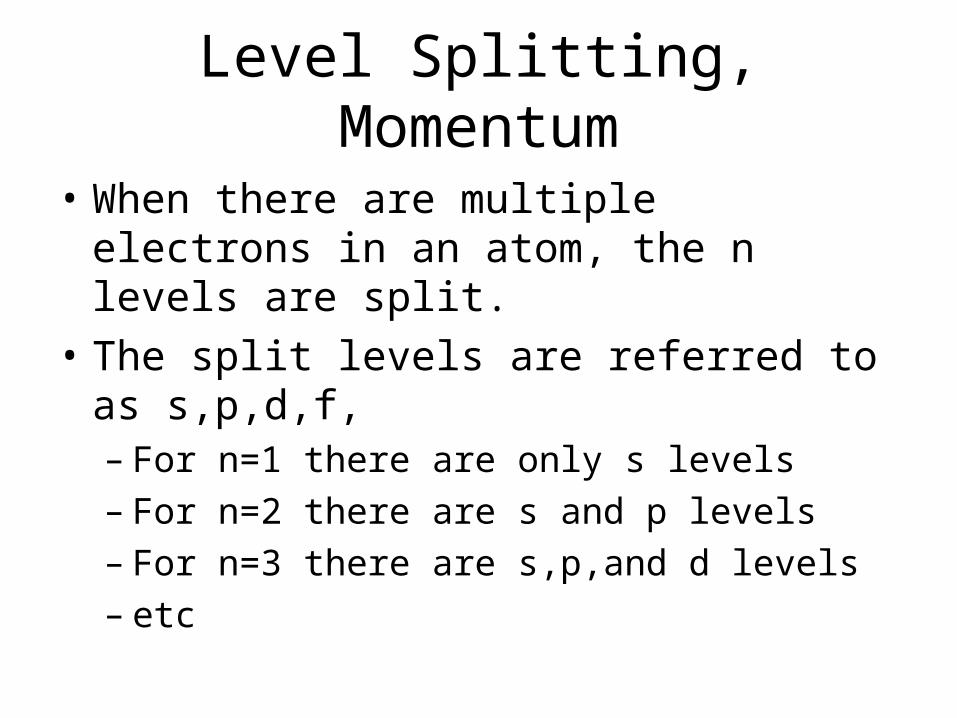
• When there are multiple electrons in an atom, the n levels are split.

• The split levels are referred to as s,p,d,f,– For n=1 there are only s levels– For n=2 there are s and p levels– For n=3 there are s,p,and d levels– etc

Spin• The other quantity is electron spin.

– He for example has 2 electrons, both can occupy the n=1 level because one has a spin of +1/2 and the other a spin of -1/2

– Transitions between spin level have a very low probability, and are referred to as forbidden transitions.

– When they are opposite to each other they are referred to as singlets

– When they are the same, triplets– Spin combined with momentum can also give

doublets.

Sample Energy Diagram

• Allowed transitions

• Forbidden transitions

• Magnetic fields can split sub-levels (ie 22s into 2 levels).

Summary

• Atomic structure - Spectral lines

• Electron transitions– N levels– Momentum s,p,d,f– Spin

• Momentum and spin splitting occurs in magnetic field – can use splitting to measure strength of field.

How to Use Spectra

• Velocity?– Doppler shift– Sometimes just an asymmetry in profile

• What else?

• Temperature – next topic

• Density – next topic

Gas State

• 1) The basic observed equation is P=NkT, N=ρ/uMH – a. This is important: if you know two, you know the third. – b. Can make observations that yield T, and ρ so you can get P.

• 2) Temperature and mean velocity – visualization again– a. Perfect box with perfect collisions: collision momentum with

wall is 2mvx – b. Number of collisions vx/2L L is size of box – c. Total of all momentum is ΣΜvx

2/L – d. Momentum is pressure so P=ML-3Σvx

2 – e. Define mean vx

2=n-1Σvx2

– f. vx2=vy

2=vz2=1/3v2

– g. P=n/3L3(Mv2)=1/3(NMv2) – h. So average energy ½ Mv2=3/2 kT This is important because it

relates energy, velocity, to temperature. (not bulk velocity)

Get The T• Velocity of atoms and electrons related to T was

just shown.• What do we need to get the temperature of the

gas? First assumption?– Assume a Maxwellian velocity distribution

• What must be assumed for this to be valid?– Collisions (not so good at very low

• f(v,T)= (M/2πkT)3/2v2e-(Mv2/2kT)

• Maxwellian tail of distribution

Line Profile Emission

– Where to measure for T?– Can get T from line width.

Boltzmann Distribution• a. Ni/N=gi/ue-ε/kT ε=hν

• b. Can use the ratio for 2 energy levels to get relative populations between two energy levels.

• c. Measure two lines from same atom to get T

• d. Ni/Nj=gi/gje-δε/kT

Saha Equation

• a. equation of ionization state:

• Ni/Nj(Ne)=(2πmkT)3/2/h3(2(ui(T)/uj(T))e-ε/kT

• b. Used to determine gas temperature

N

T

FeIII FeIV

How to Get Lines

deSI )τ()( ν

0

– I is the intensity you observe– S is emission/cm3

is optical depthis frequency– How do you get an absorption line from this?– How do you get an emission line?

Other issues

• Non-LTE

• A or f values– Line brightness– Collision prob.

• Plank function

• Differential emission measure

Log Ne2

Summary

• Spectra can give us:– T via line width, line ratios– Density via line ratios or diff. emission

measure– Velocity via line shift

MHD Equations

+H-C

– Force Balance or – Conservation of Momentum

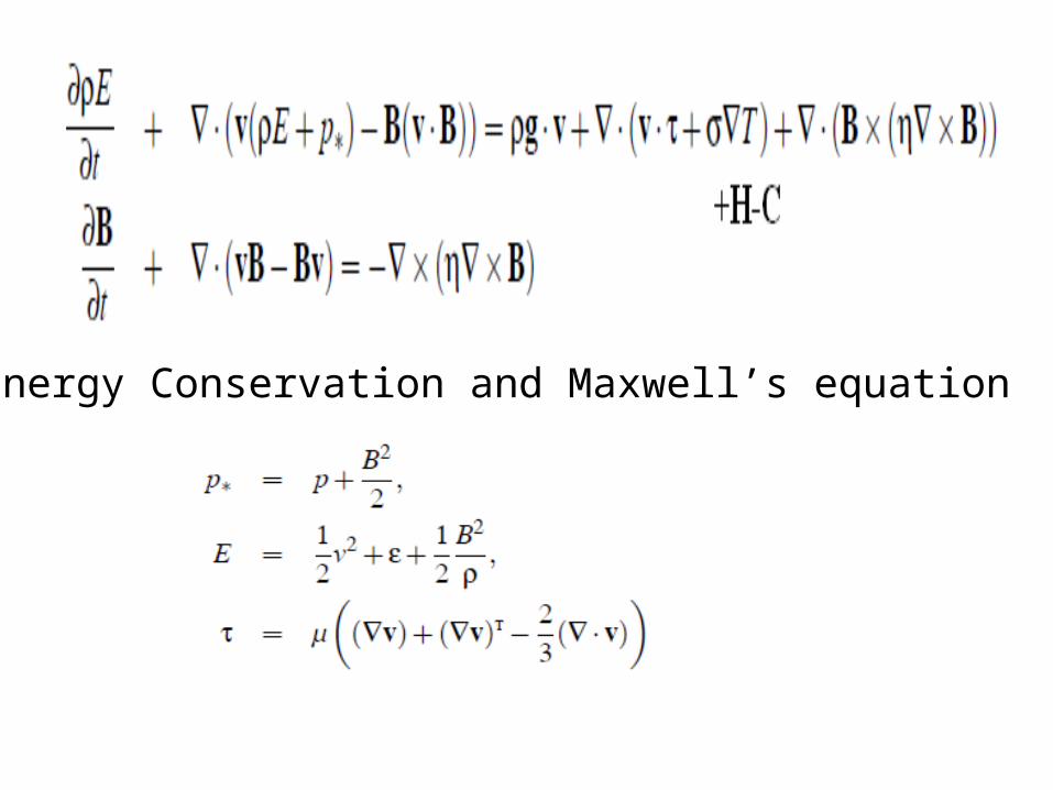
Energy Conservation and Maxwell’s equation

How to Solve

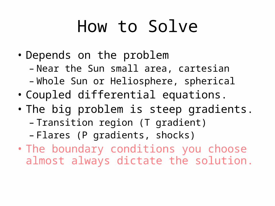
• Depends on the problem– Near the Sun small area, cartesian – Whole Sun or Heliosphere, spherical

• Coupled differential equations.• The big problem is steep gradients.

– Transition region (T gradient)– Flares (P gradients, shocks)

• The boundary conditions you choose almost always dictate the solution.

Results

• The output of these programs are table of numbers, T(x,y,z,t), P(x,y,z,t),etc.

• Need to visualize the results

• Need to make visualizations something that you can compare with observations.

Variable Grid MeshMajor Breakthrough

• Paramesh

• Steep T gradient in transition region.

• Almost no gradient in corona.

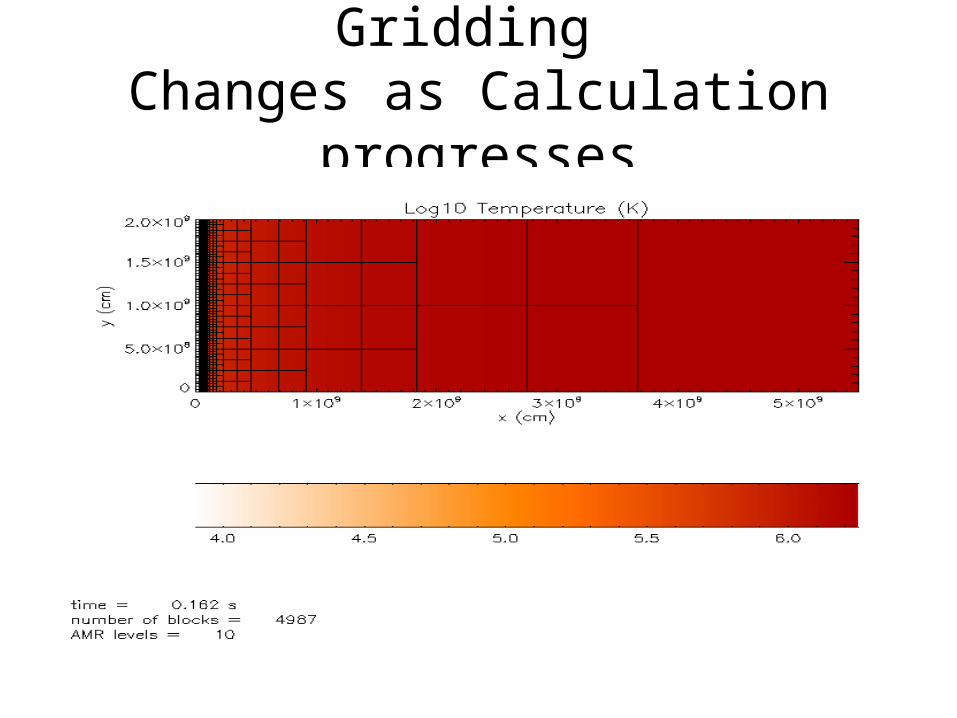
Gridding Changes as Calculation progresses

Other Issues

• Conduction– Isotropic– Anisotropic –along B field

• Radiative losses– Optically thin - collisions– Non-LTE T(collision) T(radiation)

• Heating– Constant– Alfven waves – a function of B

• Make each of these a replaceable module in your program.

Conduction• Conduction only along B field

– How the grid is oriented with respect to B

Excess heating low down

Numerical diffusion makes it wider.

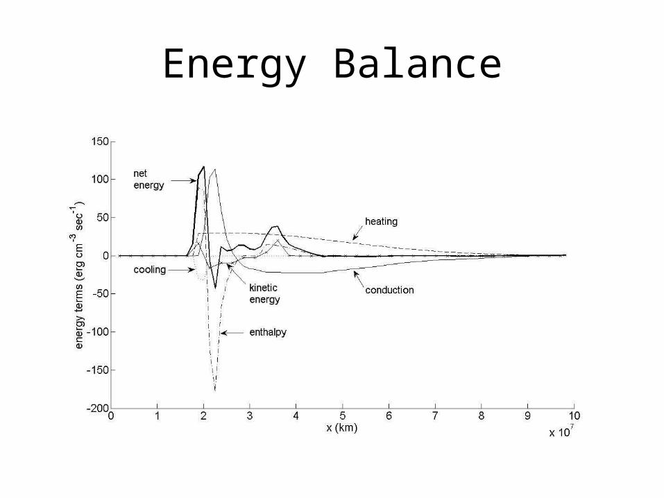
Energy Balance

Model Output

All profiles from same T different v

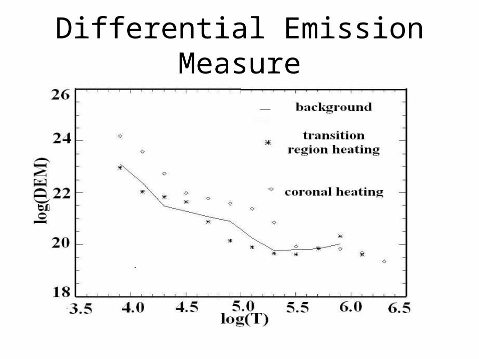
Differential Emission Measure