solar radiation modeling and simulation of multispectral satellite data

9

Solar Radiation Modeling and Simulation of Multispectral Satellite Data

Fouzia Houma1 and Nour El Islam Bachari2 1National School for Marine Sciences and Coastal Management

(ENSSMAL), Campus Dely Ibrahim Bois des Cars, Algiers Laboratory Marine and Coastal Ecosystems,

2Faculty of Biological Sciences, University of Science and Technology Houari Boumediene, USTHB, BP 32 El Alia, Bab Ezzouar Algiers

Laboratory analysis and application of radiation (LAAR) USTO, Oran Algeria

1. Introduction

All bodies emit and reflect the flow of energy in the form of electromagnetic radiation. The relative variation of the energy reflected or emitted as a function of wavelength, is the spectral signature of the object considered in a given state. The spectrum can be used to identify and determine its status. For a satellite, making measurements in a number of spectral bands, the spectral signature of an object will correspond to different levels of radioactivity recorded in each of them.

The principle of remote sensing is the detection of electromagnetic radiation that carries information from the soil-atmosphere either by reflection or by transmission from a radiometer on board the satellite. The signal received by the radiometer is the result of physical, biological and geometrical objects on the ground. For a better use of satellite measurements, we must answer the following questions: At what point on the earth's surface so far is it? What is the value of measuring that?

Answering these questions requires the definition: What exactly are the physical quantities measured by the measurement system? What disturbs the measurement system does what it is supposed to measure? Which model can you describe the disturbances? How does one characterize the quality of measurement?

To understand this complex phenomenon, we have developed an analytic model (SDDS) of radiatif transfer simulation in water coupled to an atmospheric model in order to simulate measure by satellite. This direct model permits to follow the solar radiance in his trajectory Sun-Atmosphere - Sea - Depth of sea- sensor. The goal of this simulation is to show for every satellite of observation (SPOT, Landsat MSS, Landsat TM) possibilities that can offer in domain of oceanography. (Bachari,1997)

An interaction model of the solar spectrum with the Earth-atmosphere system is developed to calculate the various components of solar radiation at ground and upper atmosphere. (Bachari, 1999; Houma and al.,2010)

www.intechopen.com

Atmospheric Model Applications 196

In this research, we are interested in applying the model to simulate the radiative transfer

through the atmosphere under realistic conditions for assessing the significance of the

effects of the atmosphere and conditions on shooting satellite images. The main objective of

this application is the analysis of satellite measurements, along with their variations

atmospheric parameters. The spectral signature of water is used here to simulate the action

of the satellites. (Gordon, 1974)

2. Modelling the interaction of the solar spectrum with the atmosphere

An analytical model for simulating radiative transfer in water coupled with an atmospheric

model can adequately simulate the signal of a body of water to the attitude of the satellite to

analyze the effects of atmospheric parameters and shallow water. This model determines the

scattered radiation by a body of water in the software simulation of satellite data SDDS

(Bachari, 1997), its main function is the calculation of the spectral radiance reflected from the

sea water level sensor.

The purpose of modeling is to understand how different components of the measurement

system combine to make a measurement. The form and content of a model depends on their

purpose. The model is constructed to describe and characterize the measurement system to

understand the phenomena which he is registered and to predict their behavior under the

effect of an external action or as a result of a partial modification of the system itself same.

The model developed is to break the middle-ground atmosphere into subsets in interaction

with the solar spectrum and the sensor onboard the satellite.

The source irradiates the object and the latter reflects the radiation in all directions, some of

this radiation is captured. The radiation received by a radiometer on board the satellite, is

composed of two main terms: brightness caused by the surface in the field of vision sensor

and a brightness that is not caused by the surface in the field of vision. The first term is

useful information, it is due to the direct and indirect solar radiation. The second term,

considered the noise is due to the light scattered by the atmosphere. (Gordon & Clark, 1981;

Becker & Rffy, 1990)

3. Spectral irradiance on the ground

The sun is the source of energy in passive remote sensing; solar radiation carries the information of the natural environment for its intrinsic properties (wavelength, polarization, phase shift). Knowledge of the spectral distribution of the radiation that reaches the high atmosphere is very important for various applications. (Chadin, 1988).The solar spectrum has been the subject of several measures on the ground, air and satellite

Assuming that the atmosphere is transparent, the solar spectrum E0λ(w.cm-2µm-1) reaching the soil does not undergo any change in its trajectory.

The spectral irradiance in the upper atmosphere depends on the latitude of the location

(latitude=ϕ), declination of the axis of rotation of the earth (δ) and time (h)

The solar spectrum on the ground is given by the following equation (Ratto, 1986 ):

Eλ = E0λ (1+f) cos (θz) (1)

www.intechopen.com

Solar Radiation Modeling and Simulation of Multispectral Satellite Data 197

E0λ : is the solar spectrum outside Earth's atmosphere, λ: wavelength of emission of radiation, 1: Astronomical Unit (1UA= 1.496x 108 km), f: is the correction factor of distance

sun-soil (this factor depends on the number of days and cos (θz) is the zenith angle).

In clear sky atmosphere, the concentration of gases and aerosols varies with the changing

weather conditions and geographical position. Gases and aerosols absorb and scatter solar

radiation on a selective basis throughout the optical path. Gases, principally ozone, carbon

dioxide and water vapor are the bodies responsible for absorption of the solar spectrum. Air

molecules and aerosols are the body responsible for the dissemination of solar radiation in

all directions. (Prieur & Morel, 1975). The effects of absorption and scattering functions are

presented by the transmittance according to Bouguer's law (Bouguer, 1953):

Tλ = Iλ/ I0λ (2)

Iλ is the spectral radiation output and I0λ is the radiation spectral λ input.

Diffusion occurs during the interaction between the incident radiation and particles or large

gas molecules in the atmosphere (water droplets, dust, smoke ...). Where the suspended

particles are negligible compared to the wavelength, the phenomenon that occurs is

Rayleigh scattering. (Fröhlich & Brusa, 1981)

The diffusion of a particle occurs independently of other particles. The radiation will be

distributed in all directions, the forward scattered radiation is equal to the radiation

scattered backward.

3.1 Model description of irradiance

This model is to calculate the solar spectral irradiance (irradiance) direct normal and

horizontal diffuse to the conditions of a cloudy sky not. This code calculates a range of 0.3

and 4.0 microns with a pitch of 10 nm. This code introduces a number of parameters such as

solar zenith angle, the angle of inclination, atmospheric turbulence, the amount of water

vapor precipitated amount of ozone, pressure and albedo (Guyot & Fagu ,1992).

Monochromatic distribution of a direct solar beam can be computed as a function of a

number of variables, including optical mass and a wide variety of atmospheric parameters-

for exemple, water-vapor content, ozone layer thickness, and turbidity parameters.

In the ultraviolet and visible region, it is essentially ozone absorption, Rayleigh scattering,

and aerosols that control attenuation of the direct beam. The transmittance by aerosols is

minimum at the short wavelengths and increases slowly as the wavelength increases. (Morel

& Gentili, 1993)

3.2 Direct spectral irradiance on the ground

The equation of the light arriving directly from the sun at ground level for a wavelength λ is

as follows:

d o r a w o uI H DT T T T Tλ λ λ λ λ λ λ= (3)

Where

www.intechopen.com


• Hoλ : represents the irradiance in the upper atmosphere of Earth-Sun distance an average wavelength λ.

• D is the correction factor for Earth-Sun distance.

• Trλ , Taλ , Twλ ,Toλ et Tuλ are respectively the functions of the transmittance of the atmosphere for a wavelength λ of molecular diffusion (Rayleigh), mitigation of aerosols, the absorption of water vapor, the absorption of ozone and gas absorption

The direct irradiation on a horizontal surface is obtained from the equation multiplied by cos (Z), or Z is the solar zenith angle:

d dI I cos(Z)λ λ= (4)

Spectral diffuse irradiance

a. The diffuse irradiance on a horizontal surface

The diffuse irradiance on a horizontal surface is based on three components:

• Component of Rayleigh scattering Irλ

• Release component aerosol Iaλ

• Component that takes into account multiple reflections of light between the ground and air

The total Isλ diffuse illumination is given by the sum.

s r a gI I I Iλ λ λ λ= + + (5)

The diffuse illumination on an inclined surface

The global spectral irradiance on an inclined surface is represented by:

[ ]{ }

[ ] ( )

T d s d o

d o

I (t) I cos( ) I I cos( ) / H Dcos(Z)

0.5 1 cos(t) 1 I / H D

λ λ λ λ λ

λ λ

= θ + θ

+ + − (6)

where

• θ is the angle of incidence of direct beam on an inclined surface

• t is the angle of the inclined surface

The angle of inclination to a horizontal surface is 0 ° and 90 ° to a vertical surface. The global irradiance on a horizontal surface is given by:

T d sI I cos(Z) Iλ λ λ= + (7)

Figures 1, 2, 3 shows the specter of global illumination DTOT, diffuse illumination DIF and direct illumination DIR.

The input parameters are:

- Optical thickness = 0.51. - Turbulence ALPHA = 1.14. - The amount of ozone O3 = 0.53 atm.cm.

www.intechopen.com


Fig. 1. Solar illumination for an area generally horizontal

Fig. 2. The solar irradiance for an area generally vertical

- Precipitable water W = 1.42 cm. - Incline angle for a surface generally vertical or horizontal : TILT = 0.0°; in the case of an

inclined surface we take the angle TILT = 60.0°; - Surface pressure 840 millibars. - The number of days in the year 96 (6 April 2009) - The number of wavelength 122 - The solar zenith angle Z = 53 °

Figure 4 shows that the maximum solar irradiance is with a solar zenith angle of 0 °, which explains when the sun is overhead (the sun is at noon) solar intensity is high and second illumination decreases with increasing solar zenith angle.

www.intechopen.com


Fig. 3. The solar irradiance for an area generally inclined

Fig. 4. Variation of solar irradiance depending on the angle of incidence.

Figure 5 shows a small optical thickness results in an intense light while a high optical thickness shows a low light, in other words, unlike the light varies with the optical thickness. (Kaufmann, and Sendra , 1992).

Figure 6 shows the variation of water vapor only affect the light weakly, but it is very important as if we compare it with the influence of the number of days in the year of the illumination.

www.intechopen.com


Fig. 5. Variation of solar Irradiance according to the optical thickness

Fig. 6. Variation of illumination depending on the water vapor precipitated.

4. Modeling the radiation reflected by the ground

In this work, we determine the physical quantity measured by the system of shooting (sensor) which is sunlight reflected by the soil-atmosphere averaged in some way in the spectral band considered the sensor. For this, we described the various factors affecting a satellite measurement.

www.intechopen.com


Thus, after characterization data on the spectrum of electromagnetic radiation, reflection, emission and atmospheric transmission is determined and developed by the optical properties of the elements of natural surfaces, radiation reflected by the surface water and radiation captured by satellites. (Houma and al.,2004)

The methods used in atmospheric modeling can be divided into direct method and indirect method. Generally, direct methods are represented by the development of a model of interaction of the solar spectrum with the various elements that are in the path of solar radiation the sun-ground and ground sensor. The radiance Lsat captured by the satellite is the sum of the three luminances:

1. The luminance of the system from the ground - atmosphere considering the ground as a black body

2. Lsol luminance reflected from the ground toward the sensor 3. Lv luminance reflected from nearby objects but observed in the direction of the ground

Lsat = La + Lsol +Lv (8)

Either a pixel image coordinate (x, y) and a spectral band b, the radiation that excites the

sensor λ K (x, y, b) (w.cm-2 µm-1 sr-1) according to Teillet (Teillet , 1986) is written as follows:

Kλ(x,y,b) = C(x,y) Rλ(x,y, b) + Hλ(b) + Δλ(x,y,b) (9)

C(x,y) is a multiplicative constant that describes the form factor that is the orientation of the

surface topography relative to the sun's position during the shooting; R(x, y, b) is the

radiation reflected by the ground is proportional to the average reflectance of the pixel (x, y)

in the spectral band b; Hλ (b) is the distribution of soil-atmosphere (noise) by considering the

earth as a black body and Δλ (x, y, b) represents a residual variable that creates the effect of

neighborhood.

R (x, y, b) is given by the following equation:

Rλ(x,y,b)=Sλ(b)Tλ(b)Gλ(b) ρλ(x,y) (10)

Sλ(b) : represents the gain factor of the system in the channel b (sensor sensitivity),

Tλ(b) is the atmospheric transmittance of the earth to the satellite in channel b,

Gλ(b) : is the global radiation and ρλ(x,y,b) : reflectance of the pixel (x, y) (assumed

Lambertian) in the channel b.

Using a database of spectral signatures and spectral extinction coefficients to model

parameters. A numerical code to track the signal in the solar sun-trip ground and ground

sensor.

The energy quantity Rλ(x,y,b) is transformed into a numbered account, which includes all information about the Earth-atmosphere system, the geometric conditions of shooting and optical properties of the sensor.

It is obvious that the atmospheric absorption and scattering vary across an image due to

three effects:

www.intechopen.com


• Change in weather conditions across an image.

• Change of observation relative to the position of the sun.

• Variation in the average radiation in the area surrounding the pixel observed at all times.

It is therefore necessary to analyze different types of information in order to quantify and qualify. (Becker,1978). To do this, we should dissect the process of taking an image, estimate its multiple components and determine at what level the various categories of information can be determined follow atmospheric correction models . (Bukata et al.,1995)

4.1 Simulation analysis of the reflectance of sea water

This model is followed by a detailed study of factors affecting the optical properties of sea water. To correctly interpret satellite data, we must solve the equation of radiative transfer soil-atmosphere. Solving the transfer equation is based on atmospheric models at several levels that require a considerable mass of meteorological data generally not available.

The first test is performed to explain the blue sky, was made by Lord Rayleigh that the assumptions of his theory are: the particles are small compared to the wavelength, the scattering particles and the medium does not contain free charges (not conductive), therefore, the dielectric constant of the particles is almost the same as that of the medium.

In vertical viewing, then the reflectance is lower than when the sun is at its zenith . The set of simulated data depends on the reflectance and the spectral amplitude of the radiation that reaches the ground is maximum at the zenith, so the measure is more affected by radiation than because of the dependence of reflectance of the zenith angle.

The zenith angle determines the illumination received by the target surface and is involved in all elements of calculating the various transmittances and radiation. Radiation received, for all channels, decreases if the solar zenith angle tends to a horizontal position; it is maximum when the sun is at its zenith . The zenith angle is involved in all elements of calculating the various transmittances and radiation, it depends on the latitude, the inclination of the sun and time.

The information spectral radiometers are determined by the wavelengths recorded by the sensor. The width of each spectral band radiometer defined spectral resolution. We consider that the observation is made in a plane perpendicular to the direction of the grooves.

Solar radiation travels through space as electromagnetic waves. In the case where the wave propagates in a medium refractive index and suddenly she meets any other medium characterized by a different index of refraction, part of the wave is then transmitted into the second medium and the other part is reflected in the first medium. The amplitude of the reflected wave depends on the nature of the medium, shape and lighting conditions.

Part of the global radiation reaching the ground is reflected to the sensor by the coefficient of reflectance. The major problem in determining the reflected radiation is the development of a model that generates all the soil properties affecting in a direct spectral signature (lighting condition, roughness, soil type,....) or indirect (color , salinity, humidity, etc.).

www.intechopen.com


4.2 Total radiation reaching the satellite

The luminance level of the satellite is the sum of the intrinsic brightness of the atmosphere and the luminance of the target which represents the sea water in our case. The radiation recorded at the satellite is given by the relation

B= (1/π) [( C(x,y)Tλ(b)Gλ(b)ρλ(x,y)(1-sρλ(x,y))+Hλ(b))Sλ(b)dλ/ Sλ(b) dλ (11)

(1/π) is a normalization factor, Tλ(θv) transmittance of direct radiation toward the sensor,

s : spherical albedo of the atmosphere et S(λ)sensitivity function optical sensor (Sturm, 1980).

The sensor has a spectral response δλ ,the recorded signal at the sensor is the luminance:

0 zatm a

0

I I cos L T d

∞λ λ λ

λ λ

ρ θ = + ρ δ λ π π (12)

The luminance level of the satellite is the sum of the intrinsic brightness of the atmosphere and the luminance of the target which represents the sea water in our case. (Deschamps et al., 1983)

The radiation reflected from the water surface to the satellite passes through the atmosphere

in a direct way with an angle θv and undergoes attenuation before being captured by the satellite.

( ) esatG I . 'λ λλ = τ (13)

eI λ : radiation reflected from the surface of the water; 'λτ : total spectral transmittance

The amount of energy that reaches the satellite sensor is the sum of that from the ground and scattered by the atmosphere. The radiation emitted by the sea water that reaches the sensor is:

( ) ( )e da drsol atmR I ' ' ' /λ λ λ λ− = τ + τ + τ π (14)

The radiation scattered by the atmosphere:

( )

o zaatm sat

I .cosR λ

λ−

ϑ= ρ

π (15)

Radiation reaching the satellite is composed of spectral global radiation reflected from the

sea water passing through the atmosphere R(sol-atm)) and part of the radiation scattered by the atmosphere R(atm-sat) . (Bricaud ,1988)

So the radiation that reaches the sensor is expressed:

( ) ( )sol atm atm satR R Rλ − −= + (16)

The signal of sea water recorded at the sensor is:

www.intechopen.com


2

1

e atm o za

I ' I .cosL d

λλ λ

λ λ λ

λ

τ ϑ = + ρ δ λ π π (17)

with : Lλ : Radiation calculated in sea water for the canal λ.

Δλ : Spectral band of the channel.

δλ : Sensitivity of the channel.

5. Simulation of satellite data for SDDS

Based on this physical model, we developed a simulation system of satellite data to correct the scattered radiation of atmospheric effects.

A library of spectral signatures is introduced, it covers the main ground objects that have a

reflectance in the bands of the electromagnetic spectrum. The combination of spectral

signatures and different radiances allows us to calculate the spectral radiance reflected from

the surfaces. The simulation results depend on the choice of input parameters. The software

allows to show the influence of the effects of various parameters and geometric

characteristics of the structures on the signal reaching the sensors onboard the satellite

SPOT, LANDSAT and IRS1C.

To highlight the effect of a given parameter on the satellite measurement, are assigned fixed

data for all variables in the case of a clear sky and for geometrically well defined.

The second part is from satellite SPOT, LANDSAT and IRS1C, applying the method of covariance matrix (a method that can provide a correction locally specific in the sense that it relates to the pixels of a given region of the image), one can estimate the atmospheric noise through a program to input data images from different channels and outputs the atmospheric noise of these channels.The physical quantity measured by the shooting system (sensor) is a solar radiation reflected by the soil-atmosphere averaged in some way in the spectral band considered the sensor. It depends on angle of illumination and shooting.

To determine the different radiation received at the satellite, the data input parameters are astronomical, geographical and atmospheric.

5.1 Atmospheric correction of remotely sensed data

Atmospheric correction is a major issue in visible or near-infrared remote sensing because the presence of the atmosphere always influences the radiation from the ground to the sensor.

As introduced before, the atmosphere has severe effects on the visible and near-infrared radiance.

First, it modifies the spectral and spatial distribution of the radiation incident on the surface.

Second, radiance being reflected is attenuated.

Third, atmospheric scattered radiance, called path radiance, is added to the transmitted radiance.

www.intechopen.com


The atmosphere transmittance is:

参飼 = 撮姉使岫−滋察伺史岫飼岻⁄ 岻 (18)

Where τ is the atmospheric optical thickness and θ can be sonar zenith angle or satellite

angle view.

The optical thickness is composed of:

酵碇 = 酵銚碇 + 酵眺碇 + 酵鳥碇 (19) 酵銚碇: Thickness selective absorption 酵眺碇: Thickness scattering by small particle (molecular) is named Rayleigh diffuse 酵鳥碇: Thickness scattering by medium particle is named Mie diffuse

For a given spectral interval, the solar irradiance reaching the earth's surface is

継直 = 完岫継聴劇沈Cos岫件岻 + 継鳥岻穴膏碇鉄碇迭 (20)

The scattering is dominated by aerosols while back scattering is mainly due to Rayleigh

scattering. A number of path radiance determination algorithms exists. For a nadir view as

Landsat MSS, TM and SPOT HRV are usually used. In this section, we only tried to

introduce some basic concepts of this complex topic. This is only a single-scattering

correction algorithm for nadir viewing condition. More sophisticated algorithms which

count multiple-scattering do exist. Some examples of these algorithms are LOWTRAN7, 5S

(Simulation of the Satellite Signal in the Solar Spectrum 5S) and 6S (Second Simulation -

aircraft, altitude of target).

There are FORTRAN codes available for these algorithms. The 5S and 6S are proposed by

Tanre (Tanre et al., 1990).

For small wavelengths the atmospheric contribution is very important, we wish to point out

that the impact angle is also important he was noticed by a degradation of the signal that

reaches the sensor signals for all contributors to the signal exciting the radiometer. The

simulation analysis shows the need to correct the satellite images of atmospheric effects in

order to identify objects on the ground. (Figure7)

The composition of the atmosphere disturbs the path of electromagnetic radiation between

the source on the one hand, between the earth and the satellite on the other. Atmospheric

effects resulting absorption and diffusion, performed jointly by the two major components:

gases and aerosols.

When a signal is recorded, it is the part of the spectral radiation scattered by air molecules

and aerosols to the outside of the system soil – atmosphere (Popp, 1994).

This signal Hλ(b) is called atmospheric noise :

Hλ(b)=E(λ)Tat-sat(λ) (21)

www.intechopen.com


Fig. 7. Contribution of the atmosphere on the multispectral channels SPOTXS.

Tat-sat(λ) is the spectral transmittance of the atmosphere, such that its optical path is calculated by replacing the zenith angle from the viewing angle.

To dissect the effects of the various elements contributing to satellite measurements, we developed a software simulation of satellite data (SDDS) using the visual language Basic.6. The tool is based on modeling of radiation and atmospheric effects. The monitoring of the solar spectrum as a double drive-ground and ground sun-sensor is implemented based on the concepts of codes 5S, 6S, to simulate different radiances reaching the sensor. For the operation of the system we used the extinction coefficients of the solar spectrum in the developed Lowtran.6 and a bank of spectral signatures extracted from the software ENVI.4.3 (2007).

6. Analysis of variation in luminance

The physical quantity measured in the system shooting (sensor) is a solar radiation reflected by the soil-atmosphere averaged in some way in the spectral band considered the sensor. It depends on the angle of illumination and shooting. (Bachari et al., 1997)

Fig. 8. Simulation of the scattered radiation as SDDS

www.intechopen.com


Fig. 9. Simulation of the spectral irradiance of water, ozone and gas as SDDS

Fig. 10. Simulation of the spectral irradiance on the ground as SDDS.

6.1 Effect of solar zenith angle

The zenith angle is involved in all aspects of calculation of the various transmittances and radiation, it depends on the latitude, the inclination of the sun and time.

cos(θz) = cos(δ).cos(latitude).cos(15(12-heure)) + sin(latitude)sin(δ) (22)

The zenith angle determines the illumination received by the ground and involved in all

aspects of calculation of the various transmittances and radiation. Radiation received, for all

satellite channels, decreases if the solar zenith angle tends to a horizontal position, and is

maximum when the sun is at its zenith (Figure 11). The following figure shows the contrast

angle (zenith-sun) radiances:

www.intechopen.com


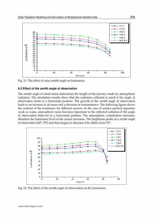
Fig. 11. The effect of solar zenith angle on luminance.

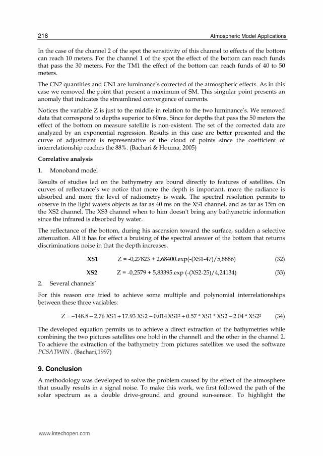
6.2 Effect of the zenith angle of observation

The zenith angle of observation determines the length of the journey made by atmospheric radiation. The simulation results show that the radiation collected is small if the angle of observation tends to a horizontal position. The growth of the zenith angle of observation leads to an increase in air mass and a decrease in transmittance. The following figure shows the contrast of the luminance for different sensors. In the case of surface spectral signature weak as water, atmospheric noise becomes important to the reflected radiation if the angle of observation believed to a horizontal position. The atmospheric contribution increases, therefore the luminance level of the sensor increases. The brightness peaks at a zenith angle

of observation [60°, 70°] and then begins to decrease if θV differs from 70°.

Fig. 12. The effect of the zenith angle of observation on the luminance.

www.intechopen.com


6.3 Effect of relative humidity

The presence of water vapor in the atmosphere depends on the location and altitude above the ground. Analysis of simulated data shows the insensitivity of the channels XS1, XS2, TM1, TM2, TM3, MSS4 to increase or decrease of water vapor in the atmosphere.The transition from a dry to a humid atmosphere causes a slight decrease in the extent to channel XS3 and TM4. Constructors radiometers onboard satellites SPOT and LANDSAT have avoided the windows of absorption of radiation by water vapor.

The following figure shows the change in apparent radiance between the two extreme amounts of water vapor. (Figure 13)

The apparent radiance level of the system SPOT, LANDSAT is practically independent of the wet state of the atmosphere because the spectral bands used do not contain the total absorption window of radiation by water vapor.

Fig. 13. The effect of relative humidity on the radiance.

6.4 Effect of diffusion parameter Fc

Mie scattering has a significant influence on the measured signal at the sensor described by the diffusion parameter Fc. The atmosphere absorbs in the field of short wavelength and becoming more transparent. The information is degraded in the channels depending on the diffusion parameter Fc. (Figure14). The following figure shows that for low surface reflectance as the case of water degradation in the channel becomes more comparable, especially for channels XS1 and MSS4.

7. Correction of satellite images

Each pixel of an image is a digital count from 0 to 255, which translates into a color using an editable pre-selected distribution in image processing. Generally the relationship between digital count and the luminance is linear:

1 0 a . CN a= +K(x,y) (23)

www.intechopen.com


Fig. 14. The effect of atmospheric turbidity parameter Fc on the radiance.

with factors a1 and a0 are calibration coefficients.

For the same conditions of image capture, simulation of the observed brightness is determined by the relationship between apparent brightness and simulated the account corresponding digital images processed.

For the three channels of the HRV sensor, radiometric conversion is given by the relations:

CNXS1 = 1.23 LXS1 + 0.22 (24)

CNXS2 = 1.24LXS2 - 0.08 (25)

CNXS3 = 1.32 LXS3 -0.59. (26)

Application to images

The same method was applied directly to the accounts of digital Landsat 2003 and Spot 2004. The images are processed using the software to process satellite images PCSATWIN developed by (Bachari et al, 1997)

Fig. 15. SPOT XS1 image before and after radiometric correction.

www.intechopen.com


Fig. 16. Landsat TM1 image before and after radiometric correction.

Calculation of the reflectance

The luminance is happening to global satellite is expressed by the relation:

L = a ρ+ b . (27)

With ρλ is the reflectance at the sea surface, E is the total illumination received by the surface. The average reflectance is connected to the luminance by the following equation:

a CN bρ = + (28)

The conversion factors obtained by modeling of radiation on SPOT satellite channels (XS1, XS2, XS3 and) and Landsat (TM1, TM2, TM3 and TM4) are given in the table below: (Bachari,2006)

Channel XS1 XS 2 XS 3 TM1 TM2 TM3 TM4

a 0. 0024 0,0025 0,0031 0,0017 0,0033 0,0026 0,0036

b − 0,05 −0,0433 −0,0217 − 0,099 − 0,0723 − 0,0416 − 0,0295

Table 1. Conversion factors accounts simulated digital reflectance.

Quality of radiometric corrections

According to the criterion Rouquet, we can estimate the quality of the correction by comparing the properties of the raw images and corrected. (Morel & Prieur, 1977) For a given image, the atmospheric effect is minimum if the contrast and the ratio of standard deviation is the average maximum, this quantitative criterion is also applied systematically for the selection of good quality data and is also a primary method of atmospheric correction, which tends to minimize atmospheric effects.

There is also a primary method of atmospheric correction, which tends to minimize atmospheric effects. The properties of the images are combined and corrected in the following table ( Bachari,1999)

For a simple analysis of the results expressed in Table 2, we note that the criterion used is justified for the corrected images. The application of atmospheric corrections is shown in the

www.intechopen.com


Fig. 17. The digital count –reflectance at ground level

Image CNmin CNmax CNmax- CNmin Ecart-type (σ) Moyenne (m) V=(σ/m)*100

XS1 Brute 38 254 216 18,23 65,10 28

XS1 Corrigée 29 255 226 24,99 38,76 64

XS2 Brute 25 235 210 21,04 55,26 38

XS2 Corrigée 11 255 244 32,80 58,58 56

XS3 Brute 17 213 206 26,40 57,85 46

XS3 Corrigée 14 255 241 37,28 67,39 55

Table 2. Statistical data of radiometric channels SPOT HRV.

graph defining the linear relationship between the reflectance calibration and account for two-channel digital SPOT XS1 and XS2 for images corrected and uncorrected images (Figure18).

0 5 0 1 0 0 1 5 0 2 0 0 2 5 0 3 0 0

0 , 0

0 , 2

0 , 4

0 , 6

0 , 8

1 , 0

1 , 2

1 , 4 x s 1 n c

x s 1 c o r

x s 2 n c

x s 2 c o r

Ré

fle

cta

nc

e

C o m p t e N u m é r i q u e

Fig. 18. Linear calibration reflectance before and after atmospheric correction.

www.intechopen.com


This simple method of correction amounts to replacing the linear calibration another linear relationship applied to both SPOT images, this new relationship calibration results to correct the measured reflectances.

Fig. 19. XS1 image of the Bay of Oran

Fig. 20. XS1 corrected image of the Bay of Oran

The statistical properties of the corrected images are presented in the following histograms:

Fig. 21. Histogram spread between raw images and images corrected SPOT.

180

190

200

210

220

230

240

250

1 2 3

XS BRUTE

www.intechopen.com


Corrected images and spectra of radiation have a greater spread and therefore a high contrast, this justifies the first condition of Rouquet.

Fig. 22. Coefficient of variation of the three images corrected for atmospheric effects.

Fig. 23. Radiometric correction in the SPOTXS1 channel of the bay of Algiers.

Fig. 24. Radiometric correction in the SPOTXS2 channel of the bay of Algiers.

0

10

20

30

40

50

60

70

1 2 3

XS BRUTE

www.intechopen.com


Fig. 25. Radiometric correction in the SPOT XS3 channel of the bay of Algiers.

In the histogram of the coefficient of variation we wish to point out that the first channel has a high coefficient corrected this can be explained as the effect of correction is more experienced in this channel than in the other two channels. In the third channel (NIR), Mie scattering and Rayleigh are less experienced.

Images are acquired by satellite sensors (HRV pour SPOT 2) (B1 (green: 0.50 – 0.59 microns), B2 (red: 0.61 – 0.68 microns), and B3 (near infrared: 0.78 – 0.89 microns).

8. Modelling of satellite measure under sea water

The knowledge of the topography of the seafloor is important for several applications. The principle of measure of bathymetry necessarily takes this model of reflectance joining the intensity of radiometric signal measured by the satellite to the depth as a basis; it can call on the physical method that requires the knowledge of all parameters governing this model (optic properties of water, coefficient of reflection of the bottom, transmittance of the atmosphere (Minghelli-Roman et al.,2007). The model provides of image mono channel where each pixel of the maritime domain is represented either by a radiometry in-situ but rather by a calculated depth. In general the use of hybrid multiple SPOT band regression algorithms are superior to the exclusive use of any single band. (Bachari & Houma 2008, Houma et al.,2010)

The spectral distribution of the submarine radiance varies in a complex way with the depth, in relation with the selective character of the attenuation.

The total signal received by a sensor operating at high altitude water above can be decomposed in a first time, in two terms:

t a eS S Sλ λλ= + (29)

with sS λ is an atmospheric component and eS λ is a water component

In a second time, it is possible to analyze the composing water measured near the surface:

e s d fS S S Sλ λ λ λ= + + (30)

www.intechopen.com


with sS λ a specular reflection at the surface, fS λ

is a reflectance of the bottom in shallow

waters, dS λ a component owed to the diffuse reflection by volume water.

( )

( )

e s s 0 a z vs s

s a z v

1 1S G G . 1 1 R exp( kz cos cos

G 1 R exp kz(cos cos )

λ λ λ

λ

= ρ + ρ ω − − − − ϑ + ϑ ρ ρ

+ − ρ − ϑ + ϑ

(31)

with ρλ a reflectance of the sea water, Ra, a reflectance of the bottom, k, is attenuation

coefficient, z, a depth, ω0 albedo of diffusion of water molecules, θz a zenith angle and θv a viewer angle of the sensor.

Fig. 26. A variation a luminance’s of a SPOT XS with a depth

Fig. 27. A variation a luminance’s of a LANDSAT TM with a depth.

0,00

10,00

20,00

30,00

40,00

50,00

60,00

70,00

0 5 10 15 20 25 30 35

Profondeur (m)

Lu

min

an

ce W

m

XS1

XS2

XS3

0

10

20

30

40

50

60

70

0 5 10 15 20 25 30 35

Profondeur (m)

LU

min

an

ce W

m

TM1

TM2

TM3

TM4

www.intechopen.com


In the case of the channel 2 of the spot the sensitivity of this channel to effects of the bottom can reach 10 meters. For the channel 1 of the spot the effect of the bottom can reach funds that pass the 30 meters. For the TM1 the effect of the bottom can reach funds of 40 to 50 meters.

The CN2 quantities and CN1 are luminance’s corrected of the atmospheric effects. As in this case we removed the point that present a maximum of SM. This singular point presents an anomaly that indicates the streamlined convergence of currents.

Notices the variable Z is just to the middle in relation to the two luminance’s. We removed data that correspond to depths superior to 60ms. Since for depths that pass the 50 meters the effect of the bottom on measure satellite is non-existent. The set of the corrected data are analyzed by an exponential regression. Results in this case are better presented and the curve of adjustment is representative of the cloud of points since the coefficient of interrelationship reaches the 88%. (Bachari & Houma, 2005)

Correlative analysis

1. Monoband model

Results of studies led on the bathymetry are bound directly to features of satellites. On curves of reflectance’s we notice that more the depth is important, more the radiance is absorbed and more the level of radiometry is weak. The spectral resolution permits to observe in the light waters objects as far as 40 ms on the XS1 channel, and as far as 15m on the XS2 channel. The XS3 channel when to him doesn't bring any bathymetric information since the infrared is absorbed by water.

The reflectance of the bottom, during his ascension toward the surface, sudden a selective attenuation. All it has for effect a bruising of the spectral answer of the bottom that returns discriminations noise in that the depth increases.

XS1 Z = -0,27823 + 2,68400.exp(-(XS1-47)/5,8886) (32)

XS2 Z = -0,2579 + 5,83395.exp (-(XS2-25)/4,24134) (33)

2. Several channels’

For this reason one tried to achieve some multiple and polynomial interrelationships between these three variables:

Z 148.8 2.76 XS1 17.93 XS2 0.014 XS1² 0.57 * XS1 * XS2 2.04 * XS2²= − − + − + − (34)

The developed equation permits us to achieve a direct extraction of the bathymetries while combining the two pictures satellites one hold in the channel1 and the other in the channel 2. To achieve the extraction of the bathymetry from pictures satellites we used the software PCSATWIN . (Bachari,1997)

9. Conclusion

A methodology was developed to solve the problem caused by the effect of the atmosphere that usually results in a signal noise. To make this work, we first followed the path of the solar spectrum as a double drive-ground and ground sun-sensor. To highlight the

www.intechopen.com


contribution of different elements making up the signal that reaches the sensor. Simulation software satellite data is developed.

The proposed radiometric correction method is simple because it is based on pixels that are known to support their radiometric images. The luminances are simulated using the software (SDDS) which allows us to establish rules between reported digital luminance and luminance reflectance. The techniques of normalization of images are to correct the atmospheric degradation, the effects of illumination and variations in the responses of the sensors in the multitemporal and multispectral imaging. Thus the methods developed in this section may be modified or combined as required by the user.

10. References

Bachari N.E.I., Belbachir A.H ., et Benbadji N.,1997 .Numerical Methods for Satellite Imagery Analysis, AMSE.,J Volume.38, N°1,2, pp 49-60.

Bachari N.E.I., et Houma F., 2005. Combination of data soils and data extracted of satellites images for the survey of the bay of Algiers, MS’05 Rouen, 6-8 Juillet 2005,France.

Bachari N.E.I., et Houma F., 2008.Contribution of satellites visible and infrared images for the follow-up of the inshore water quality; International Conference on “Monitoring & Modeling of Marine pollution” (INCOMP 2008); KISH 1-3 /12 2008

Bachari N.E.I.,1999. « Méthodologie d’analyse des données satellitaires en utilisant des données multi-sources » Thèse de Doctorat d’état en Physique; Rayonnement-Matière, 11 avril 1999, Oran USTO, Algérie.222p.

Becker F., 1978. Physiques fondamentales de la télédétection. Ecole d'été de physique spatiale C.N.E,S.

Becker F., et Rffy M., 1990. Modèles et modélisation en télédétection, Télédétection spatiale: Aspects physiques et modélisation., pp 37-162, Toulouse, Cepadues-édition, 1032 pages.

Bougeur P., 1953. Essai d'optique sur la graduation de la lumière Ann.Pys.8 Bukata R.P., Jérome J.H., Kondratyev C., and Poszdnyakov D.V., 1995. Optical properties and

remote sensing of inland and coastal waters. CRC Press, Boca Raton, Florida Chadin A.,1988. Les modèles d’interaction rayonnement-atmosphère et détemination de

paramètres météorologiques et climatologiques à partir d’observation satellitaires. Télélédétection spatiale : Aspects Physiques et Modélisation, Cepadues Editions, p 1031.

Deschamps P.Y., Herman M., and Tanré D., 1983. Modeling of the atmospheric effects and its application to the remote sensing of ocean color. Appl. Opt., 22: 3751-3758

Gordon H.R., et Clark D.K., 1981. Clear water radiances for atmospheric correction of Coastal Zone Color Scanner imagery », Appl. Opt., no 20, p. 4175-4180.

Guyot G., and Fagu X.,1992. Radiometric corrections for quantitative analysis of multispectral, multitemporal and multisystem satellite data, Int, J, Remo.Sens .

Houma F., Abdellaoui A., Bachari N.E.I., and Belkessa R., 2010.Contribution of Multispectral Satellite Imagery to the Bathymetric Analysis of Coastal sea bottom. Application to Algiers bay, Algeria. Journal Physical Chemical News, volume 53, P57-61.

Houma F., R. Belkessa, Khouider A. Bashar NIS, and Z. Derriche, 2004. Correlative Study of Physico-chemical parameters and satellite data to characterize IRS1C water

www.intechopen.com


pollution. Application to the Bay of Oran, Algeria. Water Science , volume 17 / 4, 429-446.

Kaufmann Y.J., and Sendra C., 1992. Algorithm for automatic corrections to visible and near-IR satellite imagery Int.J .Rem.Sens., 9, 1357-1381.

Minghelli-Roman A., Polidori L., Mathieu-Blanc S., Loubersac L, and François Cauneau ., 2007. Bathymetric Estimation Using MeRIS Images in Coastal Sea waters .IEEE Geoscience and Remote Sensing Letters, Vol. 4, No. 2, April 2007

Morel A. and Gentili B., 1993. Diffuse reflectance of oceanic waters; II: Bidirectional aspects. Applied Optics, vol. 32,p. 6864-6879.

Morel A., and Prieur L.,1977. Analysis of variations in ocean color. Limnology and Oceanography, vol. 22, no 4, p. 709-722.

Popp T., 1994. Atmospheric correction of satellite images in the solar spectral range, J. Research. Centre.

Prieur L., Morel A., 1975. Relations théoriques entre le facteur de réflexion diffuse de l’eau de mer, à diverses profondeurs, et les caractéristiques optiques. UGGI. XVIe Ass. Gle. Grenoble. Août 1975. Symposium Interdisciplinaire d’Optique Océanique.I.S.30, n°13 : 250-251.

Ratto C.F., 1986. Sun-earth astronomical relationships and the extraterrestrial solar radiation. Université di Genova.

Sturm B.,1980. “Optical properties of water applications of remote sensing to water quality determination”, dans G. Fraysse (dir), Remote Sensing Applications in Agriculture and Hydrology. Balkema, Rotterdam, p.471-495.

Tanre D., Deroo C., Duhaut P., Herman M., Morcette J.J., Perbos J., Dechamps P.Y.,1990. Technical note, Description of a computer code to simulate the satellite signal in the solar spectrum: The SSSSS, Int, J. Rem. Sens, 11, 659-668.

Teillet P.M., 1986. Image correction for radiometric effects in remote sensing. Int. J. Remote sensing, Vol. 7. No.12, pp 1637-1651.

www.intechopen.com

Atmospheric Model ApplicationsEdited by Dr. Ismail Yucel

ISBN 978-953-51-0488-9Hard cover, 296 pagesPublisher InTechPublished online 04, April, 2012Published in print edition April, 2012

InTech EuropeUniversity Campus STeP Ri Slavka Krautzeka 83/A 51000 Rijeka, Croatia Phone: +385 (51) 770 447 Fax: +385 (51) 686 166www.intechopen.com

InTech ChinaUnit 405, Office Block, Hotel Equatorial Shanghai No.65, Yan An Road (West), Shanghai, 200040, China

Phone: +86-21-62489820 Fax: +86-21-62489821

This book covers comprehensive text and reference work on atmospheric models for methods of numericalmodeling and important related areas of data assimilation and predictability. It incorporates various aspects ofenvironmental computer modeling including an historical overview of the subject, approximations to landsurface and atmospheric physics and dynamics, radiative transfer and applications in satellite remote sensing,and data assimilation. With individual chapters authored by eminent professionals in their respective topics,Advanced Topics in application of atmospheric models try to provide in-depth guidance on some of the keyapplied in atmospheric models for scientists and modelers.

How to referenceIn order to correctly reference this scholarly work, feel free to copy and paste the following:

Fouzia Houma and Nour El Islam Bachari (2012). Solar Radiation Modeling and Simulation of MultispectralSatellite Data, Atmospheric Model Applications, Dr. Ismail Yucel (Ed.), ISBN: 978-953-51-0488-9, InTech,Available from: http://www.intechopen.com/books/atmospheric-model-applications/solar-radiation-modeling-and-simulation-of-multispectral-satellite-data

© 2012 The Author(s). Licensee IntechOpen. This is an open access articledistributed under the terms of the Creative Commons Attribution 3.0License, which permits unrestricted use, distribution, and reproduction inany medium, provided the original work is properly cited.

http://creativecommons.org/licenses/by/3.0

solar radiation modeling and simulation of multispectral satellite data

Documents