1

Solar tracking for a parabolic dish used in a solar thermal Brayton cycle

W.G. le Roux

Study leaders: T. Bello-Ochende, J.P. Meyer

Department of Mechanical and Aeronautical Engineering, University of Pretoria

Abstract Solar thermal Brayton cycles utilise concentrated sun rays and can be used to power micro-turbine generators. For this study a 4.8 m diameter parabolic dish reflector with rim angle of 45° is required for an experimental setup to reflect sun rays onto a receiver which heats the working fluid. Two-axis tracking is required to align the parabolic dish with the sun. In this paper the method of tracking for the experimental setup is discussed. A pole and slider mechanism is used with an electronic sensor which allows the parabolic dish to follow the sun throughout a typical day. Proposed experimental results from the solar tracker show the power usage of the tracking motors throughout the day and the tracking error. The effect of the tracking error on the available solar heat rate for absorption by the receiver is investigated further with the use of SolTrace. Results from SolTrace show the maximum heat flux on the receiver as a function of tracking error. A conclusion is made on whether the tracking error for the pole and slider mechanism used in the experimental setup is acceptable or not, and on whether tube burnout can result from the tracking error. Keywords: solar, tracking, parabolic, dish, sensor Nomenclature A Area, m2 C Constant, W d Receiver aperture diameter, m D Diameter, m Gr Grashof number h Heat transfer coefficient, W/m2K k Thermal conductivity, W/mK L Length, m m& System mass flow rate, kg/s Nu Nusselt number Pr Prandtl number Q& Heat rate, W

*Q& Rate of intercepted heat at receiver cavity, W

lossQ& Rate of heat loss from the cavity receiver, W

netQ& Net rate of absorbed heat, W T Temperature, K U Radiation heat loss coefficient w Wind speed, m/s W& Power, W

Greek Letters β Receiver inclination angle σ Error µ Dynamic viscosity, kg/m·s Subscripts 0 Environment a Receiver aperture c Compressor cond Due to conduction conv Due to convection D Based on receiver diameter f fluid in At the inlet ins Insulation net Net output nrad Due to natural convection and

radiation nconv Due to natural convection optical Optical rec Receiver tube s Surface slope Slope specularity Specularity sph Spherical receiver t Turbine w Receiver inner wall

2

1. Introduction and background 1.1. The open and direct solar thermal Brayton cycl e South Africa, like Southern Africa, has much potential to generate large amounts of its power from solar technologies. Concentrated solar power systems use the concentrated power of the sun as a heat source to generate mechanical power. Mills (2004) reviewed various advanced solar thermal electricity technologies with an emphasis on new technology and new market approaches. According to Mills (2004) Brayton cycle micro-turbines appear to be moving quickly to displace Stirling engines in the two-axis tracking market because of much lower cost. The open Brayton cycle uses air as working fluid, which makes this cycle very attractive for use in the water-scarce Southern Africa. The small-scale solar thermal Brayton cycle with thermodynamically optimised components (Le Roux et al., 2011, Le Roux et al., 2012a, Le Roux et al., 2012b) could be used as a power source in the near future. The open and direct solar thermal Brayton cycle is shown in Fig. 1. The parabolic dish (concentrator) is used to reflect and concentrate the sun’s rays onto the receiver aperture so that the solar heat can be absorbed by the receiver. The heat is then transferred to the working fluid (air). The compressor increases the air pressure before the air is heated in the receiver. The compressed and heated air expands in the turbine which produces rotational power for the compressor and the load. The recuperator allows hot exhaust air to preheat the air before it enters the receiver. The rim angle of the parabolic dish determines where its focal point is. It is important that the surface profile of the dish is shaped correctly. An experimental setup for a small-scale open and direct solar thermal Brayton cycle is underway at the University of Pretoria. The aim of the work is to test experimentally the performance of the open and direct solar thermal Brayton cycle equipped with thermodynamically optimised receiver and recuperator and to compare the results with analytical work.

Compressor

Recuperator

Load

Air in 1

Air out

3

6

4

7

8

9 10

ctnet WWW &&& −=

Receiver

11

5

*Q&

2

Turbine

Figure 1. The open and direct solar thermal Brayton cycle.

1.2. Solar tracking A two-axis tracking system is required for the experimental setup of the open and direct solar thermal Brayton cycle to ensure that the sun’s rays stay focused on the receiver throughout a typical day. Many different types of solar trackers can be identified from the literature. Mousazadeh et al. (2009) reviewed different types of sun-tracking systems with their advantages and disadvantages. The most efficient and popular sun-tracking device is in the form of polar-axis and azimuth/elevation types. Mousazadeh et al. (2009) divides tracking systems into passive and active systems where the active systems are divided into micro-processor and electro-optical sensor based, auxiliary bifacial solar cell based, date and time based or a combination of sensor and date/time based (see Brooks, 2005). Date and time based trackers are dependent on geographical location of the solar dish. The passive solar trackers found in the literature are described by Clifford and Eastwood (2004), who developed a solar tracker using bi-metallic strips which reacts to solar radiation with thermal

3

expansion. According to Clifford and Eastwood (2004), two identical cylindrical tubes filled with a fluid under partial pressure can be used for a passive tracker. Active trackers are found mostly in the literature. Feuermann et al. (2002) describes the use of a tracker with an average accuracy of ± 0.05° with es sentially continuous tracking motion used in their solar fibre-optic mini-dish concentrator with 200 mm diameter. Chong and Wong (2009) describe an azimuth-elevation tracking system with a parabolic dish. According to Chong and Wong (2009), two most commonly used configurations in two-axis sun-tracking systems are azimuth-elevation and tilt-roll (or polar) tracking systems, where azimuth-elevation trackers are among the most popular sun-tracking systems employed in various solar energy applications. According to Chong and Wong (2009), the accuracy of the azimuth-elevation tracking system highly relies on how well the azimuth-axis is aligned to be parallel with the zenith-axis. Arbab et al. (2009), developed a computer tracking system of a solar dish with two degrees of freedom by using a camera to obtain the optimized picture of a bar shadow on a screen by solar dish displacements. Al-Soud et al. (2010) developed a parabolic solar cooker with a two-axis tracking system (azimuth-elevation), using a programmable logic controller. Naidoo and van Niekerk (2011), managed to build a tracking system for a solar parabolic trough with control software to rotate the trough to an optimal position with respect to the position of the sun. Two-axis tracking control using a micro-processor is described by Helwa et al. (2000). Al-Naima and Yaghobian (1990) describes a 2 m2 two-axis solar tracker controlled by a micro-processor. Pattanasethanon (2010) describes the use of a digital solar position sensor for solar tracking. A phototransistor configuration with screens and shades were employed as a detector of solar beam radiation. The height of the screen determined the sensitivity operation or period of tracking in this solar tracker. Another tracking system identified from the literature using photosensitive sensors is Hu and Yachi (2012). Nuwayhid et al. (2001) developed a simple solar tracking concentrator for a parabolic dish with diameter of 200 cm using sensors and motors. Argeseanu et al. (2009) describes the use of photoresistors in a tracking system. From the literature, typical solar tracking errors of 0.1° – 0.3° (Helwa et al., 2000), 0.2° (Brooks, 2005), 0.4° (Naidoo and van Niekerk, 2011), 0.6° – 0.7° (Chong and Wong, 2009), less than 1° (Al-Naima and Yaghobian, 1990), 1° ( Argeseanu et al., 2009) and ±1 - 2° commercially (Stafford et al., 2009) were identified. Stafford et al. (2009) found that error due to wind loading is also a measurable quantity. Yang et al. (2010) analysed defocusing phenomenon and the effect of tracking error for a parabolic trough solar thermal power system with the use of Monte Carlo Ray-Trace method. Maliage and Roos (2012) used SolTrace to compare the performance of a target aligned heliostat with experimental results. Helwa et al. (2000) and Mousazadeh et al. (2009) investigated the power usages of motors for different tracking systems. 1.3. Reflectance, slope error and specularity error The concentrator has to reflect the sun’s rays onto the receiver. For a solar concentrator, good reflectance and specular reflection of the entire terrestrial solar spectrum is important (Stine and Harrigan, 1985, Janecek and Moses, 2008 and BASF, 2007). According to Stine and Harrigan, aluminium is a good candidate. Harrison (2001) made a study of reflectors available for use in solar cookers. Harrison (2001) describes aluminium foil as a good option and it is recommended primarily because of its worldwide accessibility and cost. The reflectance of aluminium foil is listed differently by various sources, ranging from less than 79% to 86%. Polished aluminium is also identified as a good material with its 91% specular reflectance. According to Stine and Harrigan (1985), the specular reflectance of any material is a function of time, regardless of the reflector. Stine and Harrigan (1985) shows that rain is good for the reflective surfaces as it increases the reflectance. According to Grossman et al. (1991), a typical slope error for a stretched membrane dish is around 3 mrad. Stine and Harrigan (1985) mentions typical errors as slope error (2.5 mrad), tracking error (4 mrad), receiver alignment error (2 mrad), specularity error (0.25 mrad) and an error on the sun’s width (2.8 mrad). According to Stine and Harrigan (1985), a typical total effective error is 6.7 mrad. According to Gee et al. (2010), typical slope errors are 1.75, 3 and 5 mrad while specularity errors range between 0 and 3.84 mrad. According to SolarPaces (2011), a typically acceptable value for specularity error for a parabolic trough mirror material is about 3 mrad.

4

In this work, the accuracy of a tracking system to be used in an experimental setup is investigated. The effect of the tracking error, as well as optical errors, on the intercepted heat rate, average heat flux, peak heat flux and surface temperature of a modified cavity receiver, to be used in the experimental setup, is also investigated. 2. Methodology 2.1. Receiver modelling The receiver modelling is done according to Le Roux et al. (2012b). A section view of the modified cavity receiver suggested by Reddy and Sendhil Kumar (2009) is shown in Fig. 2. The receiver inner surface is made up of a closely wound tube with diameter, Drec, through which the working fluid travels. The receiver tube with length, Lrec, constructs the half spherical cavity receiver and its aperture. Note that the tube is concentrically wound. An area ratio of Aw / Aa = 8 is recommended by Reddy and Sendhil Kumar (2009), as it was found to be the ratio that gives the minimum heat loss rate from the cavity receiver. The diameter of the receiver is calculated as

( ) π3/2 awsph AAD += (1)

Due to the area ratio constraint, the receiver diameter is a function of the receiver aperture diameter,

dDsph 3= (2)

Figure 2. Modified cavity receiver.

The receiver aperture diameter is calculated using Eq. (3) since Aw = DrecLrec.

π2/recrec LDd = (3)

For Aw / Aa = 8, the Nusselt number, NuD = (hnconvDsph) / k, for natural convection heat loss rate based on receiver diameter for a 3-D receiver model is calculated as a function of the inclination angle of the receiver,

( ) ( ) ( ) 425.0317.00

968.0209.0 //cos1698.0 sphwDD DdTTGrNu −+= β (4)

For Aw / Aa = 8, the ratio of radiation heat loss to convection heat loss is a function of receiver inclination and varies between approximately 0.92 and 1.46 (Reddy and Sendhil Kumar, 2008). It is assumed that

nconvlossnradloss QUQ ,,&& = for the modified cavity receiver, where U is a function of the

inclination of the receiver and varies between 1.92 and 2.46. The rate of heat loss due to natural convection and radiation is therefore

5

( ) ( ) ( ) 425.0317.0

0968.0209.0

, //cos1698.0 sphwDnradloss DdTTUCGrQ −+= β& (5)

where ( )( )0/ TTDkAC wspha −= .

With an insulation diameter of D, the rate of heat loss due to conduction is

( ) ( )( )20, /2)2/(/ DhtDDktTTQ convinsscondloss ππ +−−=& (6)

where hconv is the external heat transfer coefficient on the insulation surface. The heat loss rate from the lower part of the receiver tube which is not insulated, due to the external forced convection of wind (Kaushika and Reddy, 2000) is

2/22.4 2805.0, dwQ convloss π=& (7)

The total heat loss rate from the cavity receiver is

convlosscondlossnradlossloss QQQQ ,,,&&&& ++= (8)

The rate of heat transfer to the working fluid is defined using the Dittus-Boelter equation as

( )fsrec

recnet TTD

mkLQ −

= 4.0

8.0

Pr4

023.0µπ

π && (9)

2.2. Effect of tracking error using Soltrace

Figure 3. Example of an analysis done in SolTrace.

SolTrace is a software tool developed at the National Renewable Energy Laboratory (NREL) to model concentrating solar power optical systems and analyse their performance. SolTrace is recommended by Bode and Gauché (2012) as a free and readily available plant performance code

6

for solar receiver research. The receiver cavity is approximated in SolTrace using 10 flat surfaces since SolTrace can only plot flux maps for surfaces and cylinders, but not spheres. Figure 3 shows an example of the use of SolTrace for this paper. In SolTrace, specularity errors in the range of 0 to 15 mrad are investigated and slope errors in the range of 0 to 15 mrad are considered, to determine the effect on the performance of the modified cavity receiver. According to SolTrace, this is an optical error range of 0 to 33.5 mrad since σoptical = (4σslope

2 + σspecularity2)1/2 (10)

A tracking error range of 0° to 3° is also consider ed. The dish surface is modelled as aluminium with reflectivity of 85%. It is assumed that two tube diameters can fit in between the aperture edge and receiver edge (see Fig. 2). A direct normal irradiance of 1000 W/m2 and a pillbox sunshape is assumed in the analysis. The optimised receiver using entropy generation minimisation (Le Roux et al., 2012b), has a tube diameter of 6.05 cm and a tube length of 11.35 m so that the aperture diameter is 0.331 m and the receiver outer diameter is 0.573 m. This receiver geometry was investigated in SolTrace. A second, larger, receiver with outer diameter of 1 m was also investigated. 2.3. Stine and Harrigan An algorithm by Stine and Harrigan (1985) to determine intercepted heat rate at a cavity receiver, is also used to compare with the results found by SolTrace. According to Stine and Harrigan (1985), at the focal point of a solar concentrator, the reflected rays do not form a point but an image of finite size centred about the focal point. This is due to the sun’s rays not being truly parallel and due to concentrator errors. The larger the receiver aperture diameter, the larger the rate of heat intercepted by the receiver, *Q& . Also, the larger the aperture diameter, the larger the

heat loss rate, lossQ& , in Eq. (8). The net rate of absorbed heat, netQ& , is the intercepted heat rate

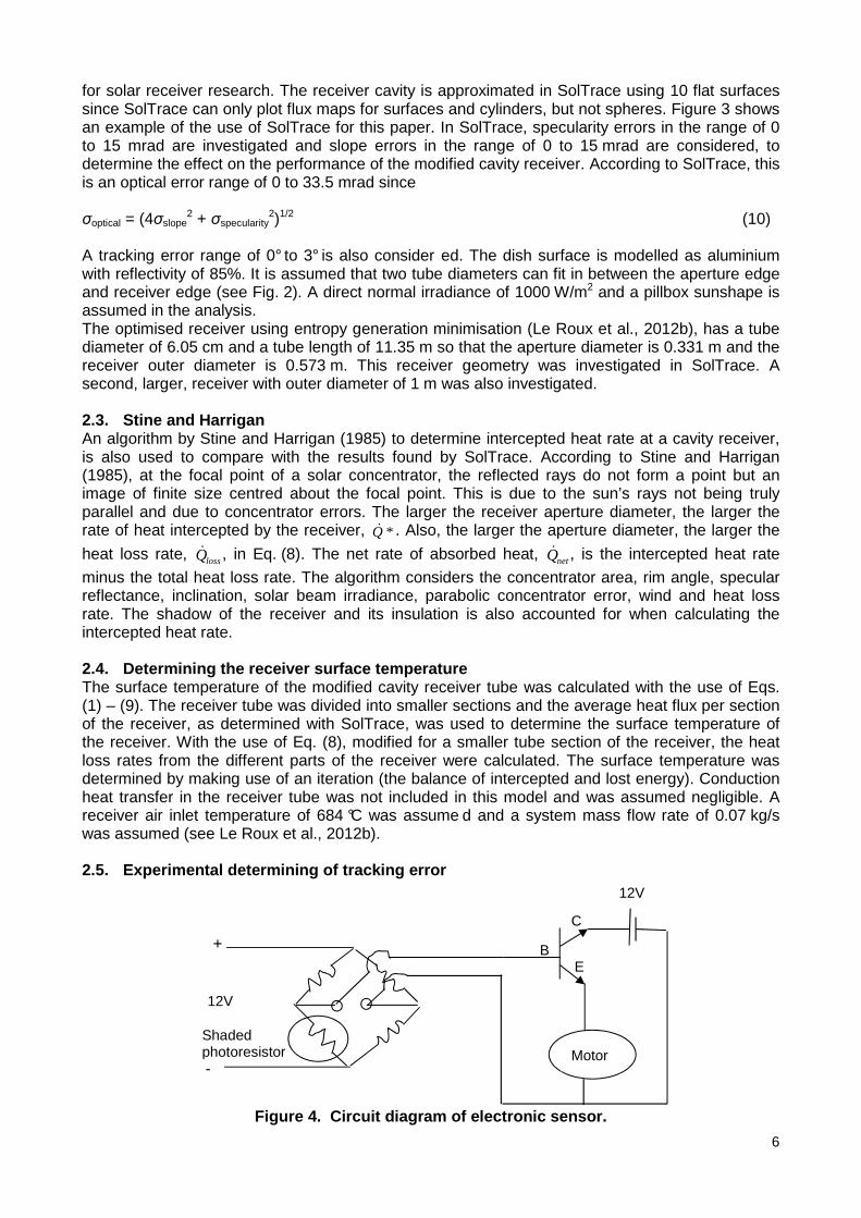
minus the total heat loss rate. The algorithm considers the concentrator area, rim angle, specular reflectance, inclination, solar beam irradiance, parabolic concentrator error, wind and heat loss rate. The shadow of the receiver and its insulation is also accounted for when calculating the intercepted heat rate. 2.4. Determining the receiver surface temperature The surface temperature of the modified cavity receiver tube was calculated with the use of Eqs. (1) – (9). The receiver tube was divided into smaller sections and the average heat flux per section of the receiver, as determined with SolTrace, was used to determine the surface temperature of the receiver. With the use of Eq. (8), modified for a smaller tube section of the receiver, the heat loss rates from the different parts of the receiver were calculated. The surface temperature was determined by making use of an iteration (the balance of intercepted and lost energy). Conduction heat transfer in the receiver tube was not included in this model and was assumed negligible. A receiver air inlet temperature of 684 °C was assume d and a system mass flow rate of 0.07 kg/s was assumed (see Le Roux et al., 2012b). 2.5. Experimental determining of tracking error

Figure 4. Circuit diagram of electronic sensor.

-

Shaded photoresistor

E

C

B

Motor

12V

+

12V

7

After considering a number of concentrator and tracking methods from the literature, with design requirements including easy maintenance, low cost, durability and light weight, a mounted pole with sliding fixed flexible concentrator, using polished aluminium segments and electronic tracking sensors was chosen. An electronic sensor was built and tested (Fig. 4). A Wheatstone bridge with four photo-resistors was used to sense where the sun was. Two resistors in the Wheatstone bridge were mounted behind a wall. The other two resistors were in direct sunlight. When the wall was not aligned with the sun, the voltage output of the Wheatstone bridge was large, because of the shade on the resistors. This signal was used to control a transistor to allow power to flow to the winch to change the position of the assembly and sensor’s position to face the sun. The advantages of this sensor are low cost and easy installation since it is self-developed. A 12 V winch was used as a motor to control the position of the assembly. Two of these trackers will be required. One sensor will track the azimuth of the sun and the other sensor the elevation. In this work, only one sensor and motor to position the assembly according to the azimuth of the sun, is tested. The setup is shown in Fig. 5.

Figure 5. Experimental setup (Circuit – left, rotat ing base – right).

Figure 6. Average flux of a 1 m diameter receiver.

0

5

10

15

20

25

30

0 5 10 15 20 25 30 35

Ave

rage

flux

(kW

/m^2

)

Position

0.0067

0.0201

0.0335

Optical error (rad)

Tracking error: 0°

0

5

10

15

20

25

30

0 5 10 15 20 25 30 35

Ave

rage

flux

(kW

/m^2

)

Position

0.0067

0.0335

0.0335

Optical error (rad)

Tracking error: 1°

0

5

10

15

20

25

30

0 5 10 15 20 25 30 35

Ave

rage

flux

(kW

/m^2

)

Position

0.0067

0.0201

0.0335

Optical error (rad)

Tracking error: 2°

0

5

10

15

20

25

30

0 5 10 15 20 25 30 35

Ave

rage

flux

(kW

/m^2

)

Position

0.0067

0.0201

0.0335

Optical error (rad) Tracking error: 3°

8

The tracking error was measured by comparing the shade line of a vertical ruler with the sensor’s centre line. This was done with the use of a protractor. The inclination and azimuth of the sun for the location of the experimental setup, for each day of the year is available from SunEarthTools (2012). 3. Results 3.1. SolTrace

Figure 7. Peak flux of a 1 m diameter receiver.

Figure 8. Average flux of a 0.57 m diameter receive r.

The average heat flux on the modified cavity receiver tube at different positions is shown in Fig. 6 for different tracking errors and optical errors. These results are for a receiver with outer diameter

0

10

20

30

40

50

60

70

80

90

100

0 1 2 3

Pe

ak f

lux

at t

he

bac

k (k

W/m

^2)

error

0.0067

0.021

0.0335

Optical error

0

50

100

150

200

250

300

350

400

450

0 1 2 3

Pe

ak f

lux

at t

he

bo

tto

m (

kW/m

^2)

error

0.0067

0.021

0.0335

Optical error

0

10

20

30

40

50

60

70

80

90

100

0 5 10 15 20 25 30 35

Ave

rage

flux

(kW

/m^2

)

Position

0.0067

0.0201

0.0335

Optical error (rad)

Tracking error: 0°

0

10

20

30

40

50

60

70

80

90

100

0 5 10 15 20 25 30 35

Ave

rage

flux

(kW

/m^2

)

Position

0.0067

0.0335

0.0335

Optical error (rad)

Tracking error: 1°

0

10

20

30

40

50

60

70

80

90

100

0 5 10 15 20 25 30 35

Ave

rage

flux

(kW

/m^2

)

Position

0.0067

0.0201

0.0335

Optical error (rad)

Tracking error: 2°

0

10

20

30

40

50

60

70

80

90

100

0 5 10 15 20 25 30 35

Ave

rage

flux

(kW

/m^2

)

Position

0.0067

0.0201

0.0335

Optical error (rad)Tracking error: 3°

9

of 1 m, and aperture diameter of 0.577 m. Position 1 - 7 is for the bottom, 9 – 20 for the bottom inner tubular wall, 21 – 28 for the upper inner tubular wall and 29 – 32 for the uppermost inner tubular wall of the receiver (see Fig. 2). Figure 6 shows that the average heat flux is mostly highest at the inner top part of the receiver, except when the tracking error and optical error is very large, which results in a large average flux at the receiver bottom. Note how increased optical error decreases the average flux at the inner top, while it increases the flux at the bottom, as the rays are spread out further away from the focal point. Figure 7 shows the peak fluxes at the back (inner top) and at the bottom of the receiver. The peak flux at the bottom is much higher, especially when the tracking error is large and optical error is small. The peak flux decreases slightly at the inner top part of the receiver as the optical error increases.

Figure 9. Peak flux of 0.57 m diameter receiver.

Figures 8 and 9 show similar results but for a 0.57 m diameter receiver with aperture diameter of 0.33 m. The results are mostly similar, except for a much higher flux at the bottom of the receiver. At large tracking errors, a small optical error further increases the flux at the bottom. The peak fluxes at the inner top and especially at the bottom are also much higher. Figure 10 compares the intercepted heat rates of the two receivers as a function of tracking error and optical error. The intercepted heat rate of the larger receiver is not much affected by the errors, while the smaller receiver’s intercepted heat rate decreases much more rapidly as the tracking error increases, especially if the optical error is also high. This is mostly because the rays miss the receiver as the error increases. This solar spillage should be avoided since it can damage the thermal insulation covering the receiver.

Figure 10. Intercepted heat rate for 1 m diameter r eceiver (left) and 0.57 m diameter receiver

(right).

0

50

100

150

200

250

0 1 2 3

Pe

ak

flu

x a

t th

e b

ack

(k

W/

m^

2)

error

0.0067

0.021

0.0335

Optical error

0

500

1000

1500

2000

2500

3000

0 1 2 3

Pe

ak

flu

x a

t th

e b

ott

om

(k

W/

m^

2)

error

0.0067

0.021

0.0335

Optical error

6

7

8

9

10

11

12

13

14

15

16

0 1 2 3

Inte

rce

pte

d h

eat

ra

te (

kW)

error

0.0067

0.021

0.0335

Optical error

6

7

8

9

10

11

12

13

14

15

16

0 1 2 3

Inte

rce

pte

d h

ea

t ra

te (

kW

)

error

0.0067

0.021

0.0335

Optical error

10

3.2. Validation The intercepted heat rates shown in Fig. 10 are compared with the results of the algorithm of Stine and Harrigan (1985) in Table 1 for the smaller receiver. It was found that the results compare well when the tracking error is small. When the tracking error is larger than 1°, the results do not compare well. This is due to the inclusion of the tracking error with optical errors, into a single total error in Stine and Harrigan’s algorithm (1985). Stine and Harrigan’s algorithm is based on the forming of an image of finite size centred about the focal point of the dish. Table 1. Intercepted heat rates calculated with Sol Trace and Stine and Harrigan. Optical error

0.0067 mrad 0.021 mrad 0.035 mrad

Tracking error

*Q& ,

SolTrace (W)

*Q& ,

Stine and Harrigan (W)

Similarity *Q& ,

SolTrace (W)

*Q& ,

Stine and Harrigan (W)

Similarity *Q& ,

SolTrace (W)

*Q& ,

Stine and Harrigan (W)

Similarity

0° 15028 14224 0.95 14794 14711 0.99 14270 16318 0.86

1° 15154 13117 0.87 14794 15073 0.95 13556 15472 0.86

2° 14892 17423 0.83 13606 16015 0.82 11443 13893 0.79

3° 11432 17669 0.45 9147 13721 0.5 7645 11327 0.52

Also note that SolTrace includes the error from the sun’s width when selecting a sun shape. According to SolTrace, specularity error is already in terms of the reflected vector and therefor the factor of 4 is included on only the σslope term in Eq. (10). Thus, SolTrace applies slope errors to the surface normal and specularity to the reflected ray. Stine and Harrigan (1985), however, define the error as

σoptical = (4σslope2 + σspecularity

2/4)1/2 (11)

It is concluded that the results of Stine and Harrigan’s algorithm (1985) compares reasonably well with the results of SolTrace when the tracking error is negligible. 3.3. Receiver surface temperature The surface temperature of the larger modified cavity receiver is shown in Fig. 11 for the different tracking errors and optical errors. The larger the optical error, the larger the receiver surface temperature at the bottom section and the smaller the surface temperature at the top section. The outlet temperatures of the air are also shown in Table 2. For the average flux assumption, the outlet temperature of the tube is 858 °C, which is close to the values shown in Table 2. The average flux assumption is a good assumption when the outlet temperature is calculated, but Fig. 11 shows that it is not a good assumption when the receiver surface temperature of the modified cavity receiver is to be determined. For the larger receiver, tube burnout at the bottom of the section should not be a problem, even at high tracking errors. The top section, however, is more vulnerable. Similar results are shown for the smaller receiver in Figure 12. It is noted that the surface temperatures are higher when the errors are small and that the temperature of the bottom section of the receiver can increase beyond the surface temperature of the top section when the tracking error is large. This temperature is then further increased when the optical error is small. For the small receiver, the tracking error shows which section would be confronted more with tube burnout. The outlet temperatures of the smaller receiver are shown in Table 3. It is noted that these temperatures are higher than those of the large receiver, except where the tracking error is too large.

11

Figure 11. Modified cavity receiver surface tempera ture (larger receiver).

Table 2. Larger receiver’s outlet temperatures. Tracking error

0° 1° 2° 3°

Optical error (mrad)

6.7 21 33.5 6.7 21 33.5 6.7 21 33.5 6.7 21 33.5

Outlet temperature (°C)

841 838 830 834 828 839 845 840 829 840 835 815

Table 3. Smaller receiver’s outlet temperatures. Tracking error

0° 1° 2° 3°

Optical error (mrad)

6.7 21 33.5 6.7 21 33.5 6.7 21 33.5 6.7 21 33.5

Outlet temperature (°C)

865 860 853 866 859 846 864 841 816 814 787 770

500

600

700

800

900

1000

1100

1200

1300

1 3 5 7 9 11 13 15 17 19 21 23 25 27 29 31

Te

mp

era

ture

(°C

)

Position

0.0067

0.021

0.0335

0.0067 (Average flux

assumption)

Tracking error: 0°Optical error (rad)

500

600

700

800

900

1000

1100

1200

1300

1 3 5 7 9 11 13 15 17 19 21 23 25 27 29 31

Te

mp

era

ture

(°C

)

Position

0.0067 0.021 0.0335

Tracking error: 3°

Optical error (rad)

500

600

700

800

900

1000

1100

1200

1300

1 3 5 7 9 11 13 15 17 19 21 23 25 27 29 31

Te

mp

era

ture

(°C

)

Position

0.0067 0.021 0.0335

Tracking error: 2°

Optical error (rad)

500

600

700

800

900

1000

1100

1200

1300

1 3 5 7 9 11 13 15 17 19 21 23 25 27 29 31

Te

mp

era

ture

(C

°)

Position

0.0067

0.021

0.0335

Tracking error: 1°

Optical error (rad)

12

It is concluded that it is useful to use SolTrace to determine the heat fluxes on the modified cavity receiver as a function of the errors to determine the surface temperatures. CFD can also be applied to determine these surface temperatures. It would be especially convenient when the peak fluxes, instead of the average flux over a certain section of the tube, are also included in calculating the surface temperatures. The assumption of constant heat flux over the whole tube length of the modified cavity receiver should be avoided when calculating the receiver surface temperature. Care should be taken when the material used for the receiver tube is selected.

Figure 12. Modified cavity receiver surface tempera ture (smaller receiver).

3.4. Experimental results Figure 13 shows the measured angle versus the real angle determined from SunEarthTools (2012) as a function of time while testing and adjusting the sensitivity of the sensor during a day. The purpose of this experiment was to determine whether it is possible to get a tracking accuracy within 2° error for the experimental setup. It was found t hat the error can be decreased by either increasing the height of the wall, increasing the input voltage of the sensor or increasing the distance between sensors. It was also found that it is important to have the azimuth-axis aligned to be parallel with the zenith-axis, as was noted by Chong and Wong (2009) in the literature. During the morning session the accuracy was within 5° - 6° (Fig. 13). It was decided to double the input voltage. During the afternoon session, the azimuth changed very quickly. It was found that the height of the shade bracket (see Fig. 5) had to be increased from 50 mm to 150 mm to keep track with the fast-moving azimuth around noon. Before starting the afternoon session, the input voltage was again doubled, which further increased the accuracy, so that the accuracy was within 2° during the afternoon session. The motor also mad e adjustments in much shorter time intervals during this session. The sensor could not be investigated further, due to time constraints. It is

500

600

700

800

900

1000

1100

1200

1300

1 3 5 7 9 11 13 15 17 19 21 23 25 27 29 31

Te

mp

era

ture

(°C

)

Position

0.0067 0.021 0.0335

Tracking error: 3°

Optical error (rad)

500

600

700

800

900

1000

1100

1200

1300

1 3 5 7 9 11 13 15 17 19 21 23 25 27 29 31

Te

mp

era

ture

(°C

)

Position

0.0067

0.021

0.0335

0.0067 (Average flux assumption)

Tracking error: 0°Optical error (rad)

500

600

700

800

900

1000

1100

1200

1300

1 3 5 7 9 11 13 15 17 19 21 23 25 27 29 31

Tem

pe

ratu

re (

°C)

Position

0.0067

0.021

0.0335

Tracking error: 1°

Optical error (rad)

500

600

700

800

900

1000

1100

1200

1300

1 3 5 7 9 11 13 15 17 19 21 23 25 27 29 31

Te

mp

era

ture

(°C

)

Position

0.0067 0.021 0.0335

Tracking error: 2°

Optical error (rad)

13

expected that the input voltage and shade bracket height will have to be further increased to ensure accuracy within 2° during the noon session a s well. The power consumption was calculated and the total power consumption for a typical day’s tracking is estimated at 12 Wh. After these experiments it was concluded that it would be possible to get the sensors to operate within 2° tracking accuracy. It is also important to note that this accuracy is much dependent on sensor alignment, base level alignment, momentum of the moving dish and also, according to Stine and Harrigan (1985), drive non-uniformity and receiver alignment. The tracking error in these experiments was mostly lagging errors. It is expected that the momentum of the dish, once installed, might decrease the error even further. This is to be investigated in future work.

Figure 13. Measured angle vs. real azimuth angle of the sun (tracking).

4. Conclusion Intercepted heat transfer rates, average heat fluxes, peak fluxes and surface temperatures of two modified cavity receivers were found for different tracking errors and optical errors of a parabolic dish assembly, using SolTrace. These results can be used to better understand the phenomenon of tube burnout and to have knowledge of the effects of typical errors. It was found that the results of Stine and Harrigan’s algorithm compared reasonably well with the results of SolTrace when the tracking error was small. It was found useful to apply SolTrace to determine the heat fluxes on the modified cavity receiver as a function of the errors. The assumption of constant heat flux over the entire length of the modified cavity receiver should be avoided when calculating the modified cavity receiver surface temperature. The constraint on the maximum allowable receiver surface temperature in the thermodynamic optimisation of the receiver geometry should be updated with this paper’s method of calculating the receiver surface temperature. A solar tracking sensor and tracking mechanism to be used in the experimental setup of a small-scale solar thermal Brayton cycle was tested and it was found to be possible to get the assembly to operate within 2° tracking accuracy. References Al-Naima, F.M., Yaghobian, N.A., 1990, Design and construction of a solar tracking system, Solar & Wind Technology, Vol. 7, No. 5, pp. 611-617.

-150

-100

-50

0

50

100

150

6 7 8 9 10 11 12 13 14 15 16 17 18

Time

Morning measurements

Noon measurements

Afternoon measurements

SunEarthTools

14

Al-Soud, M.S., Abdallah, E., Akayleh, A., Abdallah, S., Hrayshat, E.S., 2010, A parabolic solar cooker with automatic two-axes sun tracking system, Applied Energy 87 pp. 463–470. Arbab, H., Jazi, B., Rezagholizadeh, M., 2009, A computer tracking system of solar dish with two-axis degree freedoms based on picture processing of bar shadow. Renewable Energy 34, pp. 1114–1118. Argeseanu, A., Ritchie, E., Leban, K., 2009, A New Solar Position Sensor Using Low Cost Photosensors Matrix for Tracking Systems, WSEAS Transactions on Power Systems 6, Vol. 4, pp.189 – 198. BASF, The Chemical Company, 2007. Pigment for solar heat management in paints. Available at: www.basf.com/pigment. Bode, S.J., Gauché, P., Review of Optical Software for use in Concentrated Solar Power Systems. SASEC 2012, 21-23 May, Stellenbosch, South Africa Brooks, M.J., 2005, Performance of a parabolic trough solar collector, University of Stellenbosch, Dissertation. Chong, K.K., Wong, C.W., 2009, General formula for on-axis sun-tracking system and its application in improving tracking accuracy of solar collector. Solar Energy 83, pp. 298–305. Clifford, M.J., Eastwood, D., 2004. Design of a novel passive solar tracker. Solar Energy. 77, pp. 269–280. Feuermann, D., Gordon, J.M., Huleihil, M. 2002, Solar fibre-optic mini-dish concentrators: first experimental results and field experience. Solar Energy Vol. 72, No. 6, pp. 459–472. Gee, R., Brost, R., Zhu, G., Jorgensen, G., 2010, An improved method for characterizing reflector specularity for parabolic trough concentrators, SolarPaces 2010, 21-24, September 2010, Perpignon, France, Paper 0284. Grossman, J.W., Houser, R.M., Erdman, W.W., 1991, Prototype dish testing and analysis at Sandia national laboratories. SAN D91-1283C. Harrison, J., 2001. Investigation of Reflective Materials for the Solar Cooker. Florida Solar Energy Center. Available from: http://www.fsec.ucf.edu/en. Helwa, N.H., Bahgat, A.B.G., El Shafee, A.M.R, El Shenawy, E.T., 2000, Maximum Collectable Solar Energy by Different Solar Tracking Systems, Energy Sources, 22:1, 23-34. Hu, J., Yachi, T., 2012, An intelligent photosensitive tracker for concentrating PV system. International Conference on Measurement, Information and Control (MIC). Janecek, M., Moses, W.M., 2008. Optical Reflectance Measurements for Commonly Used Reflectors. Nuclear Science, IEEE. 55 (4), pp. 2432 – 2437. Kaushika, N.D. and Reddy, K.S., 2000, Performance of a low cost solar paraboloidal dish steam generating system. Energy Conversion and Management, 41, pp. 713-26. Le Roux, W.G., Bello-Ochende, T and Meyer, J.P., 2011, Operating conditions of an open and direct solar thermal Brayton cycle with optimised cavity receiver and recuperator, Energy 36: pp. 6027-6036.

15

Le Roux, W. G., Bello-Ochende, T. and Meyer, J.P., 2012a, Thermodynamic optimisation of an integrated design of a small-scale solar thermal Brayton cycle, International Journal of Energy Research, 36: pp. 1088–1104. Le Roux, W.G., Bello-Ochende, T. and Meyer, J.P., 2012b. Optimum performance of the small-scale open and direct solar thermal Brayton cycle at various environmental conditions and constraints. Energy. 46, pp. 42 – 50. Maliage, M., Roos, T.H., 2012, The flux distribution from a 1.25m2 target aligned Heliostat: comparison of ray tracing and experimental results. SASEC. Mills, D., 2004, Advances in solar thermal electricity technology, Solar Energy 76, pp. 19–31. Mousazadeh, H., Keyhani, A., Javadi, A., Mobli, H., Abrinia, K., Sharifi, A., 2009, A review of principle and sun-tracking methods for maximizing solar systems output. Renewable and Sustainable Energy Reviews 13, pp. 1800–1818. Naidoo, P., Van Niekerk, T.I., 2011, Optimising position control of a solar parabolic trough. S Afr J Sci., 107(3/4), 452. Nuwayhid, R.Y., Mrad, F., Abu-Said, R., 2001, The realization of a simple solar tracking concentrator for university research applications. Renewable Energy 24, pp. 207–222. Pattanasethanon, S., 2010. The Solar Tracking System by Using Digital Solar Position Sensor. American Journal of Engineering and Applied Sciences. 3(4), pp. 678-682. Reddy, K.S., Sendhil Kumar, N., 2008, Combined laminar natural convection and surface radiation heat transfer in a modified cavity receiver of solar parabolic dish. International Journal of Thermal Sciences, 47, pp. 1647–57. Reddy, K.S., Sendhil Kumar, N., 2009, An improved model for natural convection heat loss from modified cavity receiver of solar dish concentrator. Solar Energy, 83, pp.1884–92. SolarPaces, 2011, Measurement of solar weighted reflectance of mirror materials for concentrating solar power technology with commercially available instrumentation. Interim Version 1.1. Stafford, B., Davis, M., Chambers, J., Martínez, M., Sanchez, D., 2009, Tracker accuracy: Field experience, analysis, and correlation with meteorological conditions, IEEE. Stine, B.S., Harrigan, R.W., 1985, Solar Energy Fundamentals and Design. New York: John Wiley & Sons, Inc. SunEarthTools, 2012. SunEarthTools.com, Tools for consumers and designers of solar. Available at: http://www.sunearthtools.com/dp/tools/pos_sun [2012/10/20]. Yang, B., Zhao, J., Xu, T., Zhu, Q., 2010, Calculation of the Concentrated Flux Density Distribution in Parabolic Trough Solar Concentrators by Monte Carlo Ray-Trace Method, IEEE.