solitons, shockwaves and spikes: computational simulation ... · applied mathematical sciences,...
TRANSCRIPT

Applied Mathematical Sciences, Vol. 3, 2009, no. 59, 2933 - 2966
Solitons, Shockwaves and Spikes:
Computational Simulation of
Nonlinear Waves on Lattice
Srihari Y. Sritharan1
Brown University69 Brown St. Box 8107
Providence, RI 02912, USA
Abstract
In this paper, we systematically find computational solutions to a
class of differential equation systems which exhibit nonlinear wave be-havior. After discretizing the nonlinear partial differential equations,
we got nonlinear dynamical systems on a lattice. Using MATLAB, weutilized both an ODE and Algorithm solver method to get explicit solu-
tions with soliton and shockwave behavior. Using a 64 particle model,we plotted and animated our results in several forms, including a linear
lattice, a ring lattice (when appropriate) and phase plots. Furthermore,our use of an algorithm solver yielded three-dimensional plots of shock-wave evolution. Our calculations include the Fermi-Pasta-Ulam model,
the Toda Exponential Lattice, the Inviscid Burgers Equation and theHodgkin-Huxley Model. Using previously calculated lattices, we exper-
imented with controls and feedbacks, including the Sine-Gordon Equa-tion and the Gabov-Shefter Rosales integro-differential equation. We
concluded our research with Split Domain calculations and the intro-duction of a memory-less computation method.
Mathematics Subject Classification: 35Q51, 35Q53, 35L70, 35L65,35B37, 92C20
Keywords: soliton, shockwave, spikes, nonlinear waves, animation, com-putational neuroscience, Hodgkin-Huxley
1 Introduction
Nonlinear waves have long been an interest to scientists in a variety of disci-plines. A multitude of applications have been employed, ranging from fluid
1Srihari [email protected]

2934 S. Y. Sritharan
dynamics [9] and plasma physics [10] to even neuroscience [2, 5, 6] and biology[8]. It is with this same interest that we have chosen the topic of computa-tional waves. Waves are omnipresent, from tsunamis in the ocean, to gammawaves and sonic booms. In fact, there are currently several wave pulses propa-gating through the neurons in our brain due to the firing of action potentials.The methods and results of computational wave modeling may be adapted tofit the specifics of another field. In this paper, we will numerically solve avariety of nonlinear partial differential equations using two different numeri-cal methods in MATLAB. The first is a built-in ordinary differential equationsolver, and the second is a scheme utilizing a forward difference in time and abackward/centered difference in space. Our results include the calculations ofsolitons and shockwaves solutions, as well as spike solutions of the Hodgkin-Huxley equations from neuroscience. We will also employ controls on ourlattice and analyze the effects on wave propagation. We experiment with lin-ear and nonlinear wave propagation on a split domain lattice. We concludethe paper by devising a faster, memory-less computation method.
Calculations of the Fermi-Pasta-Ulam Model and Toda Lattice [11] com-pose Section 2. We start by introducing the Fermi-Pasta-Ulam nonlinear model[4] and simulating solitons on lattice including soliton collisions. The nonlinearterm has a variable exponent, and we solved our equation using both quadraticand cubic nonlinearities. The Toda Lattice is introduced with a brief deriva-tion. Due to its nonlinearity, we also witnessed soliton behavior in our resultsof this equation.
In Section 3, we show our calculations of the Inviscid Burgers equation.This equation produces shockwave solutions; since shocks are one of the maininterests of this paper, we utilized all of our known methods to further studythe evolution of shockwaves. We then plot the shockwave in phase space tofurther analyze its behavior.
Section 4 contains our experimentation of controls on our lattices. We firstexperimented with simple controls, such as setting a point’s position/velocityto zero. We created a control of our own which we named the ’gate control’.We moved on to feedback controls, starting with the Sine-Gordon equation[13]. We then used the Gabov-Shefter-Rosales feedback [1] and a generalizedintegral feedback, allowing for use of different kernels.
We calculated traveling spike solutions of the Hodgkin-Huxley equations[5] in Section 5. This is an application of mathematical waves to neuroscience,modeling the firing of a neuron as a voltage pulse traveling along an axon.
Split Domain problems are addressed in Section 6. In this section, we di-vided a 3000 point lattice into two parts, one governed by the Linear AdvectionEquation, and another governed by the second order wave equation (linear andnonlinear). We witnessed the behavior changes as a wave transitioned fromone region into the other.
Nonlinear waves on lattice 2935
We conclude our project in Section 7 by devising a Memory-Less compu-tation method. In this method, the code plots the current point in time whilesimultaneously solving for the next point in time. The array is then shifted,deleting the unnecessary entries of the matrix. Here, the impact of a simula-tion on the computer is greatly reduced, allowing for significantly faster andlarger simulations. The drawback, as the name suggests, is that this methodcannot remember any data before its current time step.
2 Fermi-Pasta-Ulam Nonlinear Model
In Studies of Nonlinear Waves by Fermi, Pasta and Ulam [4], they calculatedwhat are now known as ”solitons” [14] by solving a 64 point lattice governed bya nonlinear differential equation. Solitons are ”self-reinforcing solitary waves”that maintain their shape while traveling with a constant velocity. Considerthe second order wave equation with a general nonlinear term ζ(u):
∂2u
∂t2=
∂2u
∂x2+ ζ(u) (1)
When discretized in space with the centered difference, we get the following:
ui =ui+1 − 2ui + ui−1
h2+ ζi(ui) (2)
Note that in this paper, we will use the dot convention to represent totalderivatives:
u =du
dt
u =d2u
dt2
(3)
Fermi-Pasta-Ulam used the following equation in their calculations:
ζi(ui) = A[(ui+1 − ui)p − (ui − ui−1)
p]
ui =ui+1 − 2ui + ui−1
h2+ A[(ui+1 − ui)
p − (ui − ui−1)p]
(4)
Here, A and p are constants. We will use a 64 point lattice (n = 64) onwhich we will solve our equation. We will let the domain be (0, 1); since x = ih,the step size h = 1/64. We will next need to consider appropriate boundaryand initial conditions. We will use a Periodic Boundary Condition.

2936 S. Y. Sritharan
Remark 1: Periodic Boundary Conditions
Unless otherwise specified, all succeeding examples in this paper will use peri-odic boundary conditions. A periodic boundary means we set un+1 = u1 andu0 = un; in effect, this causes any wave that reaches either end of the n pointmodel to reappear on the other end.
If we consider Eq. 4 at the boundaries i = 1 and i = n, the ODE’s are nowthe following:
u1 =u2 − 2u1 + un
h2+ A[(u2 − u1)
p − (u1 − un)p]
un =u1 − 2un + un−1
h2+ A[(u1 − un)
p − (un − un−1)p]
(5)
Figure 1: Continuous Chain
Which thus sets up our n = 64 point model on a continuous chain. We nowdefine our initial conditions for the problem; let us first consider the quadraticcase (p = 2) with the following initial condition:
ui =
{
2 for i = 15, 16
0 otherwise
A = .3
(6)
If the nonlinear coefficient A is too high, the wave may blow up in finitetime. Finally, we may compile the above information into our ODE solver. Formost cases, we used the ode45 and ode113 commands in MATLAB to solveour systems. Exceptions to this will be noted specifically for each case. Ifusing the MATLAB ode45/ode113 solvers, the program can only handle firstorder derivatives, so we need to represent our second order time derivative asa system of first derivatives:
ui = vi
vi =ui+1 − 2ui + ui−1
h2+ A[(ui+1 − ui)
p − (ui − ui−1)p]
(7)
For computational simplicity, we will represent the above system in MAT-LAB by couching both u and v into one vector U:
U = (u1, . . . , un, v1, . . . , vn) (8)

Nonlinear waves on lattice 2937
After running the solver, we will get a following output: 1) a vector T,whose elements are the times for which u is solved:
T =
t1t2t3...
(9)
Y =
u1(t1) u2(t1) u3(t1) . . .u1(t2) u2(t2) . . .
u1(t3)...
...
(10)
We may plot our results in one of many ways. The first way is to plot uagainst time for all 64 particles. This produces the following graph:
Figure 2: Plot of ui vs. time
The amplitude of the particles has a near constant amplitude. This is oneobservation that may lead us to conclude that we are dealing with solitons. Aproperty of the soliton is that it keeps its shape and amplitude throughout itspropagation. Linear superposition of waves does not occur.
An animation is another useful way (and our main method) to plot ourresults; for this type of plot, time cannot be an axis, as the animation willrun in real-time. If we imagine a chain of particles, our axis for the animationmust be its horizontal position on the chain vs. its vertical displacement fromthe origin. We will therefore plot each particle with coordinates (i, ui). Sinceui is a function of time, we will fix our time, ’take a picture’ of the graph andsave it as a movie frame; by repeating this procedure for each point in time,we can compile the frames into an animation. Our output will be a movie thatruns the animation in real-time; however this is impossible to show on a piece

2938 S. Y. Sritharan
of paper. Instead we will create thumbnail indexes which show every severalframes as a picture, leaving the animation of the solution to the imaginationof the reader. Using the above concept, we will animate our solution, shownbelow as a thumbnail index:
Figure 3: Thumbnail
We see that the disturbance of points u15 and u16 results in two largewaves rather than several small ones. We can see later when they collide (3rd
thumbnail) that these two waves are indeed solitons. Another property of thesoliton is that it will collide violently with other solitons but emerge with itsshape and direction (generally) unaffected.
A very interesting case to observe is a sinusoidal initial condition (for all64 points):
ui(0) = sin(2πi
64) (11)
This time we will set our nonlinear coefficient a little higher: A=0.5.
Figure 4: Plot of ui vs. time
We can see that as time continues, the oscillations of the sine curve becomemore exotic.
Nonlinear waves on lattice 2939
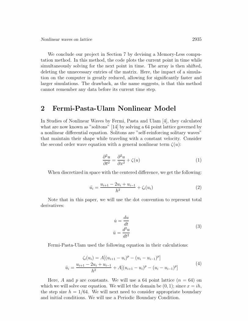
Figure 5: Thumbnail
This animation takes a very long time to exhibit its exotic behavior (com-pare the time axis length of Fig 4 to Fig 2). Therefore, in order to save space,we have shown every several hundredth frame in our thumbnail. As a result,the actual motion of the chain is difficult to follow; however, we can still ob-serve the interesting shapes of the wave. The animation begins with standingwave behavior, initially exhibiting no nonlinear activity. Soon, the standingwave begins to warp in a clockwise direction, with an almost twisting behav-ior. We can see in the thumbnails that as time continues, very interestingoscillations result, including secondary instabilities within the chain.
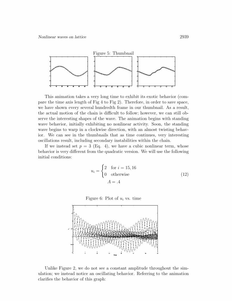
If we instead set p = 3 (Eq. 4), we have a cubic nonlinear term, whosebehavior is very different from the quadratic version. We will use the followinginitial conditions:
ui =
{
2 for i = 15, 16
0 otherwise
A = .4
(12)
Figure 6: Plot of ui vs. time
Unlike Figure 2, we do not see a constant amplitude throughout the sim-ulation; we instead notice an oscillating behavior. Referring to the animationclarifies the behavior of this graph:
2940 S. Y. Sritharan
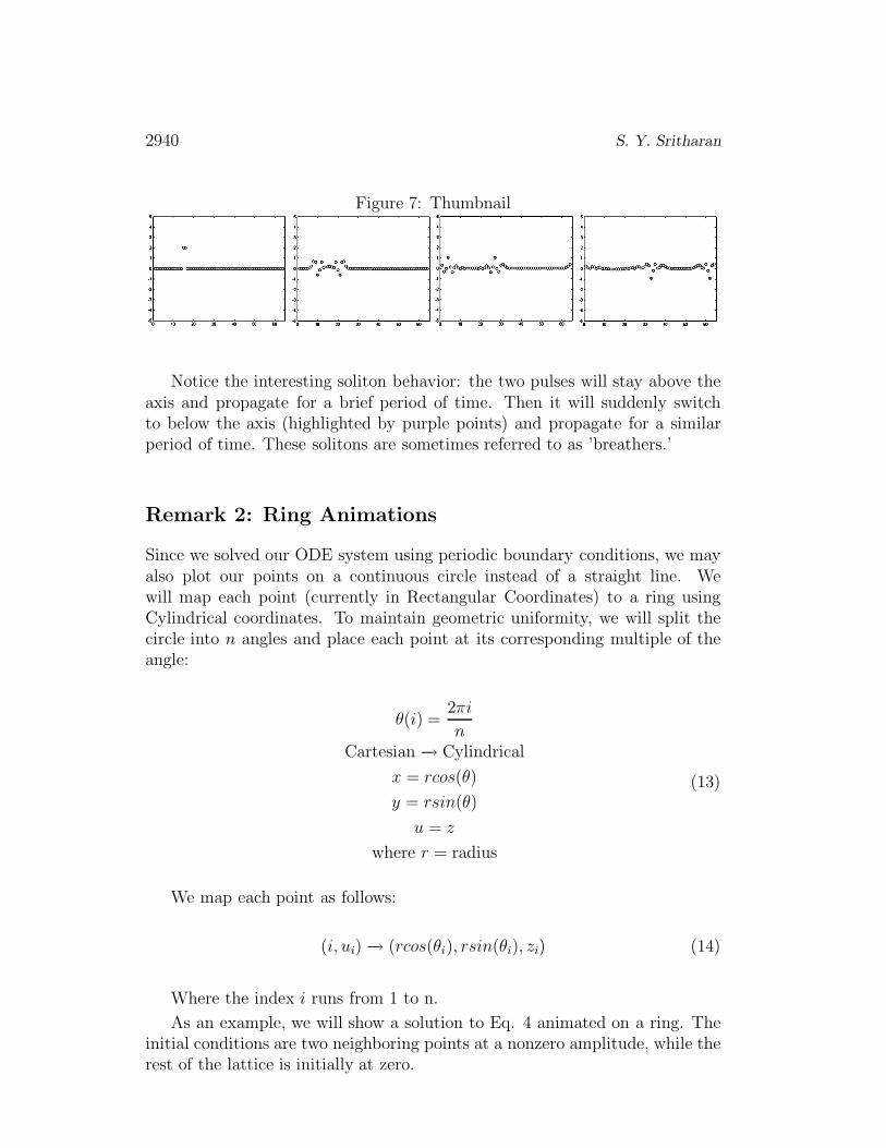
Figure 7: Thumbnail
Notice the interesting soliton behavior: the two pulses will stay above theaxis and propagate for a brief period of time. Then it will suddenly switchto below the axis (highlighted by purple points) and propagate for a similarperiod of time. These solitons are sometimes referred to as ’breathers.’
Remark 2: Ring Animations
Since we solved our ODE system using periodic boundary conditions, we mayalso plot our points on a continuous circle instead of a straight line. Wewill map each point (currently in Rectangular Coordinates) to a ring usingCylindrical coordinates. To maintain geometric uniformity, we will split thecircle into n angles and place each point at its corresponding multiple of theangle:
θ(i) =2πi
nCartesian −→ Cylindrical
x = rcos(θ)
y = rsin(θ)
u = z
where r = radius
(13)
We map each point as follows:
(i, ui) −→ (rcos(θi), rsin(θi), zi) (14)
Where the index i runs from 1 to n.
As an example, we will show a solution to Eq. 4 animated on a ring. Theinitial conditions are two neighboring points at a nonzero amplitude, while therest of the lattice is initially at zero.

Nonlinear waves on lattice 2941
Figure 8: Ring Animation of Solution to Eq.4
The waves pass the boundary at u1 , u64 without any hindrance and con-tinue to propagate along the chain. This graphically shows the observer thetopology of a periodic boundary condition.
2.1 Toda Exponential Lattice
This section solves what is known as an ”exponential lattice”: a system ofODE’s with exponential terms (instead of linear). The Toda lattice is a modelfor a 1-D nonlinear crystal modeled as a chain of particles. We will not givea detailed derivation [11], but instead will give a quick introduction. Theequation of motion for this type of system is given as follows:
md2yi
dt2= V ′(yi+1 − yi) − V ′(yi − yi−1) (15)
where yi is the displacement of each ith particle, and V is potential thatdefines the interaction between neighboring points. For example, for a linearlattice the potential V follows from Hooke’s Law:
V (yi) =k
2(yi)
2 (16)
The potential that Fermi-Pasta-Ulam used in their paper contains a non-linear polynomial term:
V (yi) =k
2(yi)
2 + ka
n(yi)
n n = 3 or 4 (17)
For the following exponential lattice, Toda prescribed the potential functionas:
V (yi) =a
be−byi + ayi + C1 (18)
Where a, b, and C1 are constants. Taking the derivative with respect to yi,we get:

2942 S. Y. Sritharan
V ′(yi) = −ae−byi + a (19)
We substitute this into our equation of motion:
md2yi
dt2= a
(
e−b(yi−yi−1) − e−b(yi+1−yi))
(20)
We define ’mutual displacement’ [11] as a new generalized coordinate asfollows:
ui = yi − yi−1 (21)
We subtract the term md2yi−1
dt2to write our equations of motion in terms of
ui :
(
md2yi
dt2− m
d2yi−1
dt2
)
= a(e−b(yi−yi−1) − e−b(yi+1−yi))
− a(e−b(yi−1−yi−2) − e−b(yi−yi−1)) (22)
Substituting Eq 21:
md2ui
dt2= a
(
2e−bui − e−bui−1 − e−bui+1)
(23)
We will set a = m and b = 1 to receive our final equation:
d2ui
dt2= 2e−ui − e−ui+1 − e−ui−1 (24)
Which we will refer to as the Toda Exponential Lattice.If we expand Eq. 24 into a Taylor Series, we get the following terms:
d2ui
dt2=
n∑
k=1
(−1)k−1
k!
(
uki+1 − 2uk
i + uki−1
)
(25)
We see that the first term of our Taylor Series (k = 1) is the discrete,linear second order wave equation (Consider Eq. 4 where A = 0). Therefore,the Toda Lattice is simply the linear wave equation plus many higher ordernonlinear terms. Similar to the Fermi-Pasta-Ulam nonlinear term, the nonlin-earities within the exponential terms can produce solitons. In fact, there areexplicit soliton solutions for the Toda Lattice; however it is beyond the rangeof this paper. For the Toda Lattice, we found computational errors with peri-odic boundary conditions; therefore, we have instead placed fixed boundaries.Consider the following initial condition:

Nonlinear waves on lattice 2943
u11(0) = u14(0) = u51(0) = u54(0) = 2
u12(0) = u13(0) = u52(0) = u53(0) = −2(26)
Figure 9: Thumbnail
Notice the soliton collision at points u32 and u33 (3rd thumbnail); similarto Fig 3, the solitons emerge generally unchanged. The Toda Lattice doesnot show significant nonlinear behavior for small disturbances, but for largerinitial conditions, a very characteristic soliton shape can be seen evolving.
3 Inviscid Burgers Equation
The Inviscid Burgers equation is a first order PDE but is very different fromthe previous equations in that it produces shock solutions.
∂u
∂t= −u ·
∂u
∂x(27)
We must take care in many ways as to how we discretize Eq. 27; otherwise, wemay have an unstable scheme. The use of any difference (backward, forward orcentered) will be unstable at zero. Therefore we must instead rewrite our PDEto allow a point to access a zero value. If we rewrite Eq. 27 as a Conservationof Mass Law, we eliminate the instability at zero.
∂u
∂t= −
∂
∂x
(
1
2u2
)
(28)
We will use both the ODE and the algorithm solver methods to furtherstudy the behavior of shockwaves.
3.1 ODE Solver and Examples
Using Eq. 28 as our PDE, we may now apply differences to create a new, morestable scheme [7]. To maintain stability, the scheme must employ backwardsdifferences for positive ui and forwards differences for negative ui.

2944 S. Y. Sritharan
ui =−1
2(u2
i − u2i−1) for ui ≥ 0
ui =−1
2(u2
i+1 − u2i ) for ui < 0
(29)
Consider the following block initial condition:
ui =
{
2 for 16 ≤ i ≤ 18
0 otherwise(30)
Before we display our results, we will explain how to analyze the anima-tions. Consider the Inviscid Burgers Equation as follows:
∂u
∂t+ u
∂u
∂x= 0 (31)
We will try to find a characteristic curve s in the x − t plane along which wecan integrate.
Figure 10: Characteristic
We then write the derivative of u with respect to s:
∂u
∂s=
∂u
∂t
dt
ds+
∂u
∂x
dx
ds(32)
Referring to the above figure, the slope of the curve s is dtdx
. Compare thisto Eq.31 and we find that:
∂u
∂s= 0
dt
ds= 1
dx
ds= u
(33)
Thus the slope of the characteristic is dtdx
= 1u. Considering the initial condi-
tion prescribed in Eq. 30, the slope from points 1 to 15 and 49 to 64 is infinity,and points 16 to 48 is 1
2.Therefore we can display the following slope field for
our initial condition:

Nonlinear waves on lattice 2945
Figure 11: Slope Field of Eq.29 and Eq.30
We see two types of interactions occurring between the two slopes. At theinteraction on the left, we see that the lines do not intersect when the slopeschange; this is known as an expansion fan. However for the interaction onthe right, we see that the lines intersect; this is known as a shock. We maytherefore generalize where an expansion fan or shock will occur:
if uleft > uright ; forms a shockif uleft < uright ; forms an expansion fan
Figure 12: Plot of ui vs. time

2946 S. Y. Sritharan
Figure 13: Thumbnail
We can see that the analysis of Fig. 11 holds for the evolution of the shock-wave in this figure. In the first thumbnail, the discontinuity on the left formedan expansion fan and the discontinuity on the right formed a shockwave.
In the case that we have multiple discontinuities in our initial condition(i.e. multiple shocks), the greater discontinuity will dominate. This meansthat as the shocks evolve, the lesser shocks will merge into the greater shock.As an example, let us consider the following initial condition:
ui =
0 if 1 ≤ i ≤ 16
1 if 17 ≤ i ≤ 32
2 if 33 ≤ i ≤ 48
3 if 49 ≤ i ≤ 64
(34)
Figure 14: Plot of ui vs. time
Nonlinear waves on lattice 2947
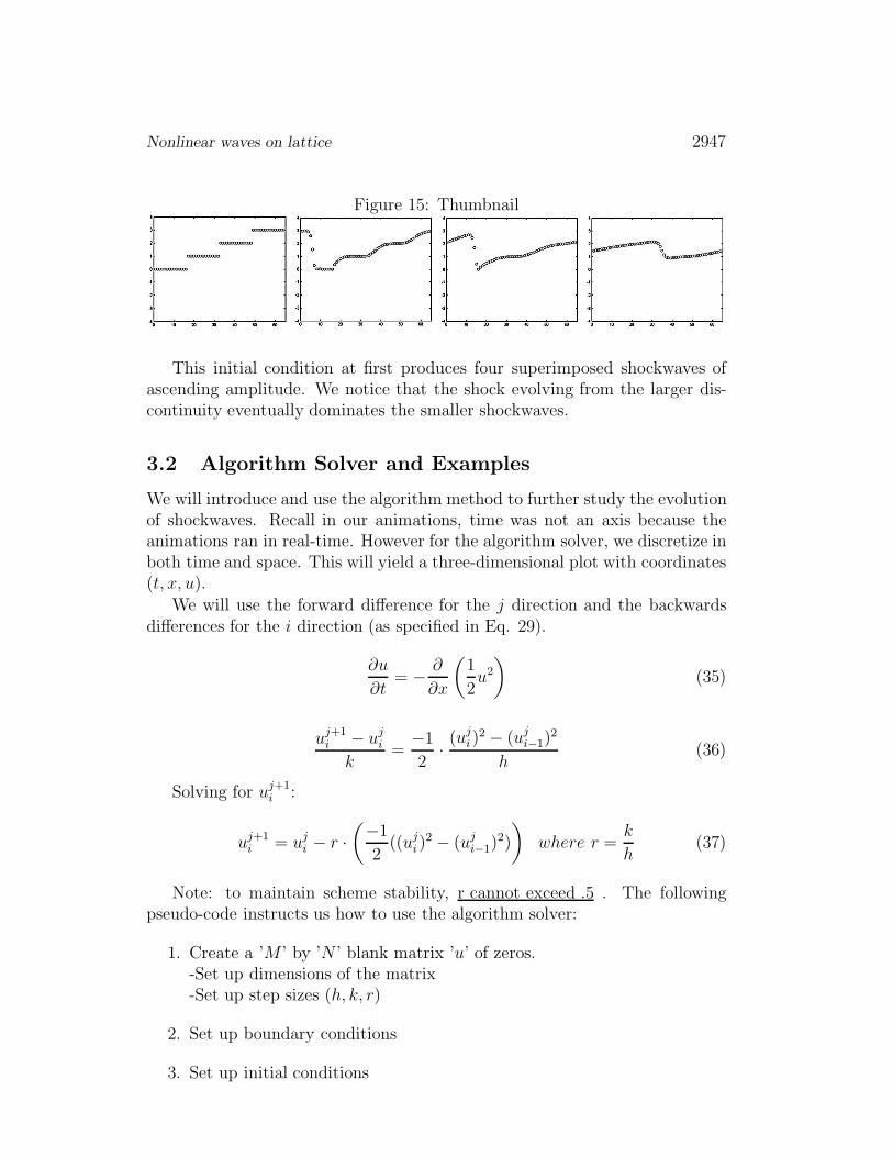
Figure 15: Thumbnail
This initial condition at first produces four superimposed shockwaves ofascending amplitude. We notice that the shock evolving from the larger dis-continuity eventually dominates the smaller shockwaves.
3.2 Algorithm Solver and Examples
We will introduce and use the algorithm method to further study the evolutionof shockwaves. Recall in our animations, time was not an axis because theanimations ran in real-time. However for the algorithm solver, we discretize inboth time and space. This will yield a three-dimensional plot with coordinates(t, x, u).
We will use the forward difference for the j direction and the backwardsdifferences for the i direction (as specified in Eq. 29).
∂u
∂t= −
∂
∂x
(
1
2u2
)
(35)
uj+1i − uj
i
k=
−1
2·(uj
i )2 − (uj
i−1)2
h(36)
Solving for uj+1i :
uj+1i = uj
i − r ·
(
−1
2((uj
i )2 − (uj
i−1)2)
)
where r =k
h(37)
Note: to maintain scheme stability, r cannot exceed .5 . The followingpseudo-code instructs us how to use the algorithm solver:
1. Create a ’M ’ by ’N ’ blank matrix ’u’ of zeros.-Set up dimensions of the matrix-Set up step sizes (h, k, r)
2. Set up boundary conditions
3. Set up initial conditions

2948 S. Y. Sritharan
4. Apply algorithm to u-Take care as to how the algorithm is applied: fix j, run i, then move tothe next step in j.
5. Plot u as a surface.
The following figure is a graphical representation of Eq. 37.
Figure 16: Algorithm Grid
This figure shows us that, using Eq. 37, knowledge of the blue points allowsus to solve for the value of the red point.
We will use a Dirichlet boundary, where the endpoints are equal to zerofor all time. By referring to Fig. 16, we can see that we will have problemson the left boundary (i.e. when uj
i is on the first column, uji−1 is accessing
a nonexistent point.). We will also run into problems at the top boundary;however this is a superficial issue. We would only need to access the topboundary if we needed values above the top row, and this is not the case.Therefore, we may simply run our code up to the second-to-top row. Sinceour wave travels to the right, we may adopt a similar solution to for the leftboundary and only run the code starting from the second column (i = 2). Wewill set our initial condition to be the following:
u1i =
{
2 if 10 ≤ i ≤ 20
0 otherwise(38)
Remembering that the point u11 is at the bottom left corner, we may run
a nested double ’for loop’ to find all the values of u. For our first plot, we willfirst make our step sizes relatively large (i.e. low resolution) and set N = 200and M = 64, where N is the number of rows and M is the number of columns.

Nonlinear waves on lattice 2949
Figure 17: Low Resolution Plot
Notice that the shock had propagated and hit the right boundary; however,there is a simple fix for this problem. A key strength of the algorithm method isthat increasing either the time or space interval does not necessarily increasethe coding complexity. All we need to do is increase the x direction of ourmatrix u, and the shock will take much longer to reach the boundary. For thenext figure, both the x and t dimensions have been increased, allowing for alonger evolution of the shock without boundary issues (N = 2000, M = 400).Also, the step size of both directions have been decreased to create an imagewith a much higher resolution.
Figure 18: High Resolution Plot
(Note: color scheme changes have no relevance with data.)
In this figure, we can see in much clearer detail how the discontinuityevolves into the sharp shockwave shape that we witnessed in our animations.

2950 S. Y. Sritharan
Figure 19: Greater Discontinuity Dominates
For this figure, our initial condition was three blocks of decreasing magni-tude. Similar to the results shown in Fig. 14, we can see that as time continues,the smaller shocks merge into the larger shock.
3.3 Phase Plot
Since our animations concern 64 particles following harmonic motion, it isrelevant to study the equilibrium points of the system. A phase plot is usedfor exactly this purpose, and is set up by plotting u against du
dt. Let us consider
a block attached to a spring with no damping. Given a displacement and aninitial velocity, the block will oscillate indefinitely. Below is a phase plot thissystem:
Figure 20: Simple Harmonic Motion Phase Plot
As we stated earlier, the system is oscillating indefinitely without approach-ing the equilibrium at the origin (denoted by a star.) If we now consider the

Nonlinear waves on lattice 2951
same system with moderate damping, the system will eventually approach itsequilibrium at (0, 0).
Figure 21: Damped Harmonic Motion
All phase plots spiral clockwise by convention. We define a phase diagramwith an inward traveling spiral (such as the above figure) as a stable equilib-rium; likewise, we will define outward spirals and saddle points as unstableequilibria. The figure below shows a phase plot of the first Inviscid Burgersexample:
Figure 22: Phase Plot of Fig.12
If we individually analyze the 64 distinct graphs for each point, we candeduce that the thick set of lines that range from (0.1, ε) to (2, ε) is the phasespace representation of the expansion, while the set of arcs below is the shock.The straight, diagonal lines that seem to be outliers represent the points at theinitial discontinuities that immediately jump to form the expansion fan/shock.As the shock passes, we see the phase lines converging upon a nontrivial equi-librium at (1, 0) i.e. at position u = 1 with zero velocity.

2952 S. Y. Sritharan
4 Controls
To conclude our project, we experimented with the effects of controls on ourlattices. Starting with simple controls, we applied a variety of controls to asecond order wave equation lattice. We later progressed to a study of feedbackcontrols; we explored the effects of the Sine-Gordon equation on the secondorder wave lattice as well as the Gabov-Shefter-Rosales feedback on the InviscidBurgers Equation.
4.1 Simple Controls
An easy control to apply is to directly affect the motion of a particle, eitherby giving a constant value or a defined function of time. The first control wewill apply is setting a particles position to zero. This is similar to a DirichletBoundary; all waves will hit the ’frozen’ point and bounce back, and no waveswill propagate past the frozen point. We will apply these simple controls to alinear second order wave equation lattice.
For our first example, we will set the following conditions:
Initial Condition: u32(0) = 1 others = 0
Control: u34(t) = 0 ∀t(39)
Figure 23: Thumbnail
As expected, we only see wave propagation on the left side, while the34th point blocks waves to the right. Notice that the 33rd point is at anequilibrium above the axis instead of at zero. This is a phenomenon seen withfixed boundaries.
If we now freeze two points instead of one, we can house the wave withinthe range of the two frozen points. We will keep our initial condition, but wewill change our control to the following:
u25(t) = 0 ∀t
u39(t) = 0 ∀t(40)

Nonlinear waves on lattice 2953
Figure 24: Thumbnail
Now, waves cannot pass point u25 or u39; in effect, we can interpret thiscase to be analogous to reducing the number of points in the lattice.
Instead of setting the position of a particle equal to zero for all time, wecan instead set its velocity equal to zero. We will set the following conditions:
Initial Condition: ui(0) = sin(2πi
64)
Control: u16(t) = u48(t) = 0 ∀t(41)
Figure 25: Thumbnail
Notice that, unlike Fig. 23 and Fig. 24, freezing the velocity of a pointdoes not create a behavior similar to a fixed boundary. Instead we notice thatwe have a rubber band effect; the neighboring points keep a sort of tensionbetween themselves and the controlled points. This is analogous to imposinga Neumann Boundary at the above said points.
We will next introduce a control that is more abstract than the previousexamples. We will first designate two points on the chain: one as a ’monitor’and another as a ’gate’. Using these points and a simple if-then condition,we may set up a sort of wave filter which we will call a ’gate control.’ Forexample, consider the following arguments:
if umonitor > C0
then ugate = 0;where C0 is a constant.

2954 S. Y. Sritharan
In the above arguments, we have established that if the value of the moni-tor point exceeds a given value, the gate point will ’shut’. In effect, this willblock any large waves from crossing the gate point. We will designate thefollowing points as an example:
umonitor = u29
ugate = u27
C0 = .25
(42)
In order to receive accurate results, we need to change our ODE solver toode23s. This solver has a much smaller time step and can deal with a logical if-
then statement in the differential equation. Using ode113/ode45 will producechoppy animations as the solver attempts to refine its time-step beyond itscapabilities.
Figure 26: Thumbnail
As another example, we will now use two gates:
umonitor1 = u29
umonitor2 = u35
ugate1 = u27
ugate2 = u37
C0 = .25
(43)
We see that waves above an amplitude of .25 are blocked on both sidesby the gates. To change the behavior of our gate, we can change the logicalargument to ’greater than’, ’(not) equal to’, etc. Also, using other operators,such as absolute value or mean value, can produce more interesting gates.
4.2 Feedback Controls
In this final section, we will briefly show two types of feedback of forces toobserve their effects on dynamics. We will first introduce the Sine-GordonEquation [13]:
∂2u
∂t2=
∂2u
∂x2+ sin(u) (44)

Nonlinear waves on lattice 2955
We see that the above equation can be regarded as Eq. 1 with ζ(u) equalto a sinusoidal feedback force. To see the effect of the feedback, we will usethe following initial condition:
for 20 ≤ i ≤ 44
ui(0) = sin(2πi− 20
24)
(45)
Figure 27: Thumbnail
Interestingly, the feedback force prevents lateral propagation of the wave.Throughout the animation, the feedback keeps it contained within the vicinityof its original location.
The Sine-Gordon equation yields very interesting results with a step as aninitial condition:
for 20 ≤ i ≤ 44
ui(0) = 1(46)
Figure 28: Thumbnail
Again, we see the feedback contains the wave within its initial region andexhibits behavior similar to a cosine standing wave. For our second feedback,we will first introduce the Gabov-Shefter-Rosales Equation [1]:
∂u
∂t= −
∂
∂x(1
2u2) +
∫ 2π
0
sin(x − y)u(y)dy (47)
Note that the above equation is the Inviscid Burgers equation with anintegral feedback. In order to discretize the above PDE, we must approximatethe integral using a sum; we will use the trapezoid rule:
where y is a dummy variable used for our integration.

2956 S. Y. Sritharan
∫ 2π
0
sin(x − y)u(y)dy =h
2[u1sin(h(i− 1)) + unsin(h(i− n))
+
n∑
j=2
2ujsin(h(i− j))] (48)
To make sure our integral limits are correct we must set up our step size asfollows:
h =2π
I(49)
where I is an integer.To prevent the wave from blowing up in finite time, we needed to set some
conditions. We will first multiply a constant in front of the integral:
A
∫ 2π
0
sin(x− y)u(y)dy = Ah
2[u1sin(h(i− 1)) + unsin(h(i− n))
+
n∑
j=2
2ujsin(h(i− j))] (50)
Recall that the direction of our difference must be switched if the valueof ui is negative. Therefore, to avoid this instability, we will shift the restingequilibrium of our points to two. We have set the following initial conditionsand constants:
ui =
{
4 if 20 ≤ i ≤ 44
2 otherwise
A = .15
h =2π
64
(51)
Figure 29: Thumbnail
Interestingly, after a long period of time, the wave will sustain a constantshape. Below is the figure at frame 1500:

Nonlinear waves on lattice 2957
Figure 30: Frame 1500
After an extended period of time, however, the shape will become unstableand collapse, producing another smaller shockwave. This wave dissipates tozero and no further behavior is seen.
We will generalize Eq. 47 so we can use many functions inside the feedbackintegral:
∂u
∂t= −
∂
∂x(1
2u2) +
∫ T
0
G(x − y)u(y)dy (52)
ui =−1
2(u2
i−u2i−1)+
h
2[u1G(h(i−1))+unG(h(i−n))+
n∑
j=2
2ujG(h(i − j))] (53)
We will call the function G our kernel. This time, we will try out two new,additional conditions: first, we will only apply the feedback to points 10 to 20,and second, we will use different kernels. Let us define the exponential kernelas follows:
G = −e−A·h(i−j)2 (54)
We will use the following initial and feedback conditions:
ui =
{
4 if 20 ≤ i ≤ 44
2 otherwise
A = .5
h = .1
(55)
2958 S. Y. Sritharan
Figure 31: Thumbnail
The feedback affects points 10 through 20 by depressing the amplitude ashighlighted in the second thumbnail. The shape is generally sustained through-out the propagation of the shockwave.
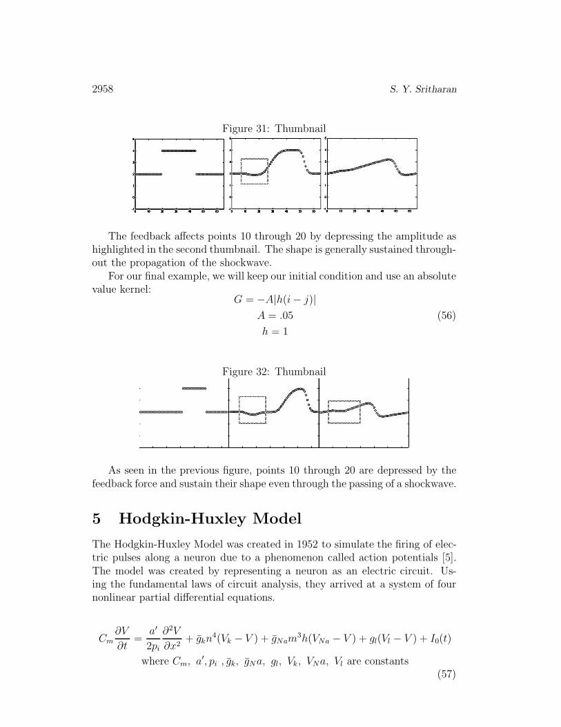
For our final example, we will keep our initial condition and use an absolutevalue kernel:
G = −A|h(i− j)|
A = .05
h = 1
(56)
Figure 32: Thumbnail
As seen in the previous figure, points 10 through 20 are depressed by thefeedback force and sustain their shape even through the passing of a shockwave.
5 Hodgkin-Huxley Model
The Hodgkin-Huxley Model was created in 1952 to simulate the firing of elec-tric pulses along a neuron due to a phenomenon called action potentials [5].The model was created by representing a neuron as an electric circuit. Us-ing the fundamental laws of circuit analysis, they arrived at a system of fournonlinear partial differential equations.
Cm
∂V
∂t=
a′
2pi
∂2V
∂x2+ gkn
4(Vk − V ) + gNam3h(VNa − V ) + gl(Vl − V ) + I0(t)
where Cm, a′, pi , gk, gNa, gl, Vk, VNa, Vl are constants(57)

Nonlinear waves on lattice 2959
∂n
∂t=
(
−.01(V + 50)
e−.1(V +50) − 1
)
(1 − n) −(
.125e.125(V +60))
n (58)
∂m
∂t= −.1
(
V + 35
e−.1(V +35) − 1
)
(1 − m) −(
4e−(V +60)
18
)
m (59)
∂h
∂t=
(
0.07e−.05(V +60))
(1 − h) −
(
1
1 + e−.1(V +30)
)
h (60)
The neuron is thought to operate using ion channels within the cellularmembrane. These channels are analogous to time and voltage dependent,nonlinear resistors in an electric circuit. So, each variable in the above fourequations represents an electric component of the circuit. The voltage is rep-resented by V , while n, m, and h are related to the behavior of the nonlinearresistors. The time dependent function I0(t) is called the injection current andis similar to a initial condition on the neuron. The neuron has voltage sensi-tive ion gates that open and close in respect to the voltage across the neuron.When a certain voltage threshold is exceeded, a voltage spike is formed withinthe membrane and travels along the axon. This process is called an actionpotential and is what the Hodgkin-Huxley model strives to simulate. Since allfour PDE’s need to be solved simultaneously, it will be unnecessarily complexif we use the ODE solver. Instead, we are going to use the algorithm solver(see section 3.2) for all four variables.
5.1 Plots
Most of the constants and conditions on this problem are experimentally de-termined; the initial conditions for V , n, m, and h are all zero. The injectioncurrent I0(t) is some nonzero value (with the correct units, usually 19.0) for asmall fixed period of time. Assuming that the wave travels from left to right,the left boundary is clamped/closed (Dirichlet Boundary) and the right bound-ary is either open (Absorbing Boundary) or closed (Dirichlet). For simplicity,we will close both ends of the axon. We are calculating on a 150 point lattice,iterating over 6000 points in time. As stated above, we will let I0 be 19.0 onthe first 30 points for 300 iterations in time. The final 50 spatial points arenot shown in the below graph because they show no significant activity in thissimulation.

2960 S. Y. Sritharan
Figure 33: Voltage Plot of Action Potential
We notice that at first, as the current is injected, the voltage in points 1 to30 steadily increases. Once a certain voltage is reached, the height drops andtransfers a wave traveling to the right. Since this wave arises from a nonlinearPDE, and the wave sustains its shape throughout its propagation, we couldconclude that this spike is a soliton. However, it can be shown that a wavecollision between two action potentials using the Hodgkin Huxley model causestotal cancellation of the waves. As we previously mentioned, a property of asoliton collision is that each soliton emerges generally unaffected. Therefore wecan conclude that this equation does not produce solitons, but simply travelingwaves with a constant shape.
Figure 34: Thumbnail of Action Potential
6 Split Domain Wave Calculations
We set up a n-point lattice with a split domain to observe the behavior ofwaves that transition between regions governed by different equations. Points1 to k (for k relatively small) is governed by the linear advection equationut = ux and points k + 1 to n are governed by the second order wave equationutt = uxx. Periodic boundaries were employed.
Nonlinear waves on lattice 2961
Figure 35: Diagram of Split Domain Lattice
The linear advection equation can be rewritten in the factored form:
∂u
∂t−
∂u
∂x= 0 (61)
(
∂
∂t−
∂
∂x
)
u = 0 (62)
Similarly, the second order wave equation can be rewritten as:
∂2u
∂t2−
∂2u
∂x2= 0 (63)
(
∂
∂t−
∂
∂x
) (
∂
∂t+
∂
∂x
)
u = 0 (64)
Since the(
∂∂t− ∂
∂x
)
operator is present in both equations, the interfaceshould allow waves to pass from one region to another.
6.1 Linear Case
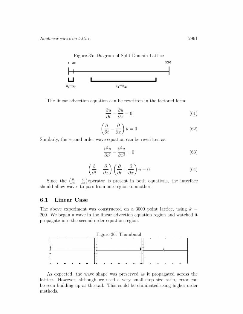
The above experiment was constructed on a 3000 point lattice, using k =200. We began a wave in the linear advection equation region and watched itpropagate into the second order equation region.
Figure 36: Thumbnail
As expected, the wave shape was preserved as it propagated across thelattice. However, although we used a very small step size ratio, error canbe seen building up at the tail. This could be eliminated using higher ordermethods.

2962 S. Y. Sritharan
6.2 Nonlinear Case
We repeated the above trial, this time using adding the quadratic Fermi-Pasta-Ulam nonlinear term to the second order wave equation, seen in Section 2.
d2ui
dt2=
ui+1 − 2ui + ui−1
h2+ A[(ui+1 − ui)
2 − (ui − ui−1)2] (65)
We used the same initial conditions, boundary conditions, and lattice sizesfrom the linear case above. However instead of preserving the wave, the non-linear region heavily distorted it, breaking it into many shock-like solitons.
Figure 37: A=0.005 (relatively small)
Unlike Fig. 3, the solitons formed here are not symmetric peaks, but sharpplateaus/shockwaves. As the wave continues to propagate, the shocks continueto split farther apart. The Inviscid Burgers equation has the property thatshocks of higher amplitudes travel with faster wave speeds. However, it wouldappear that the opposite is occurring here; the shock with the lowest amplitudeis traveling faster than any other part of the compounded wave. One canconfirm that these waves are solitons using a simple collision test; the waveformed above will travel through other solitons unchanged.
We do observe heavy error at the tail of the wave; the use of a high orderRunge-Kutta ODE solver in MATLAB slightly reduces the tail error, but thesplitting shockwave behavior is identical.
It is difficult to determine whether the shock behavior is due to error build-ing up or if this is the true solution to this case of the split domain problem.Since we do not have an analytical solution of the Fermi-Pasta-Ulam equation,we do not have anything to compare this to. We repeated this with a muchhigher nonlinear term coefficient to observe the effect.
Figure 38: A=0.017 (relatively large)

Nonlinear waves on lattice 2963
This time, the wave split into more shocks (four instead of two). The errorat the tail was even larger. The increased nonlinearity presented an interestingresult but did not help decipher the behavior any further.
7 Memory-Less Computation Method
When solving and animating a system of differential equations, a matrix isusually used to store the coordinates of each point for every point in time.After the matrix is completed, plotting methods are used to animate the data.However, accessing and saving such a large matrix over many iterations iscomputationally intensive, making big simulations impractical on a personalcomputer. Also, one must wait until the entire calculation is complete beforevisualizing the result.
To improve on this, we can instead plot the current time step while si-multaneously calculating the next time step, thus solving the system ”on-thefly”. If we use a matrix of the same size as prescribed in the original method,this would effectively increase the computational load. So to make this newmethod feasible, we must reduce the size of the matrix considerably.
Suppose that we are solving a second order wave equation problem on a npoint lattice over T points in time. Then, we would usually set up a [nX T ]matrix which we would solve by iterating over each point in time. But thesecond order wave equation only requires the knowledge of the previous andcurrent time step in order to solve the next step. Therefore, the maximumnumber of time steps ever concurrently accessed is three. We can take advan-tage of this to animate the result as it is being solved. We employ two initialconditions at two neighboring, distinct points in time, t0 and t1 . Let Zi = thesolution of the system at the point i.
1. We will create two matrices, u and v, of size [nX 3] and set the first andsecond columns of u to be the initial conditions of the problem. Thematrix v is currently all zeros.
u =
Z1(t1)(Initial Condition) Z1(t2)(Initial Condition) 0Z2(t1)(Initial Condition) Z2(t2)(Initial Condition) 0Z3(t1)(Initial Condition) Z3(t2)(Initial Condition) 0
. . . . . . . . .
(66)
2. With the knowledge of the first and second columns, we solve for thevalues of the third column of u using finite differences.

2964 S. Y. Sritharan
u =
Z1(t1)(IC) Z1(t2)(IC) Z1(t3)Z2(t1)(IC) Z2(t2)(IC) Z2(t3)Z3(t1)(IC) Z3(t2)(IC) Z3(t3)
. . . . . . . . .
and v =
0 0 00 0 00 0 0
. . . . . . . . .
(67)
3. Now we plot the third column of u and copy the values of u to v witha one column backward translation. Reset the values of u to zero. Nowwe solve v for its third column, which is the fourth step in time.
u =
0 0 00 0 00 0 0
. . . . . . . . .
and v =
Z1(t2)(IC) Z1(t3) Z1(t4)Z2(t2)(IC) Z2(t3) Z2(t4)Z3(t2)(IC) Z3(t3) Z3(t4)
. . . . . . . . .
(68)
4. We repeat step three for matrix v; plot the third column of v and copythe values of v to u with a one column translation, allowing us to solvefor the fifth time step. Reset the values of v to zero.
u =
Z1(t3) Z1(t4) Z1(t5)Z2(t3) Z2(t4) Z2(t5)Z3(t3) Z3(t4) Z3(t5). . . . . . . . .
and v =
0 0 00 0 00 0 0
. . . . . . . . .
(69)
5. Continue to solve by alternating u and v; since there is no matrix beingpermanently stored, we can iterate this loop and simulate indefinitely.
In summary, we are calculating the next time step as we simultaneouslyplot the current time step by alternating our solution matrix between two [n x3] matrices. This method could be easily adapted for higher spatial dimensionproblems.
There are many positive aspects of this ”on-the-fly” computing method.There is a greatly increased computation speed and capacity due to the de-creased virtual memory allocation. Due to the use of smaller matrices, thereis also a much faster visualization speed. Finally, we do not have to wait forthe entire simulation to complete before visualizing the result. We can there-fore stop a simulation that either blows up or does not produce the desiredresult without loss of time. There is, however, a drawback to this method:this simulation is memory-less and remembers no further than the last threetime steps. This means that we cannot numerically analyze the simulationas a whole, only visually observe the result; saving the animation would bedifficult and impractical. A way to fix this is to continually save the data in alarge matrix as the simulation is running; however, this would heavily reducecomputation speed.

Nonlinear waves on lattice 2965
Conclusion
In this project, we found results that display interesting features of nonlineardynamical systems. Many insights were gained into the behavior of solitonsand shockwaves, as well as into an application of nonlinear waves in neuro-science. Our experiments with control techniques brought forth intriguingoutcomes as well. We would like to further pursue other physiological applica-tions of this topic, such as nonlinear wave activity in the cardiovascular system.Furthermore, we wish to conduct more studies with higher order methods, es-pecially in the split domain calculations, to discover the reasons behind ourunusual results. Lastly, in the future we seek to perform calculations of theKdV and shallow water equations and simulations concerning breaking wavesin the ocean.ACKNOWLEDGEMENTS. The author thanks the University of Wyomingmathematics graduate students Saikat Mukherjee and Eric Quade for their helpin the nonlinear waves and neuroscience parts of this project, respectively.The author also thanks the following professors for the stimulating discussionsconcerning this project: Prof. Peter Lax (NYU), Prof. Roberto Camassa(UNC Chapel Hill), Prof. Long Lee (U of Wyoming), Prof. Frederico Furtado(U of Wyoming), and Prof. Frank Giraldo (Naval Postgraduate School).
References
[1] J. Boyd, A Legendre-pseudospectral method for computing travelingwaves with corners (slope discontinuities) in one space dimension with ap-plication to Whitham’s equation family, Journal of Theoretical Physics,
189 (2003), 98-110.
[2] P. Dayan, L. F. Abbott, Theoretical Neuroscience; Computing and Math-
ematical Modeling of Neural Systems, MIT Press, 2001.
[3] C. Farhat, I. Harari, U. Hetmaniuk, A discontinuous Galerkin methodwith Lagrange Multipliers for the solution of Helmholtz problems in themid-frequency regime, Computer Methods in Applied Mechanics and En-
gineering, 192 (2003), 1389-1419.
[4] E. Fermi, J. Pasta, S. Ulam, Studies of Nonlinear Problems, Collected
Papers of Enrico Fermi, Vol 2., The University of Chicago Press, 1955.
[5] A.L. Hodgkin, A. F. Huxley, A Quantitative description of membranecurrent and its application to conduction and excitation in nerve, Journal
of Physiology, 117 (1952), 500-544.

2966 S. Y. Sritharan
[6] C. Koch, Biophysics of Computation, Oxford University Press, New York,1999.
[7] R. LeVeque, Numerical Methods for Conservation Laws, Lectures inMathematics, ETH Zrich, 1994.
[8] P. S. Lomdahl, S. P. Layne, I .J. Bigio, Solitons in Biology, Los Alamos
Science, Spring (1984), 27-30.
[9] A. Newell, Reflections from Solitary Waves in Channels of DecreasingDepth, Journal of Fluid Mechanics, 153 (1985), 1-16.
[10] T. E. Sheridan, Evolution of Unstable Ion Acoustic Solitons, Plasma Sci-
ence, IEEE Transactions, 27 (Feb 1999), Issue 1, 140-141.
[11] M. Toda, Waves in Nonlinear Lattice, Supplement of the Progress of The-
oretical Physics, 45 (1970), 174-200.
[12] S. T. Thornton, J. B. Marion, Classical Dynamics: Of Particles and Sys-
tems, Thomson Brooks/Cole, 2004.
[13] E. W. Weisstein, ”Sine-Gordon Equation,” From MathWorld–A Wolfram Web Resource, http://mathworld.wolfram.com/Sine-GordonEquation.html
[14] N. J. Zabusky, M.D. Kruskal, Interaction of ”Solitons” in a CollisionlessPlasma and the Recurrence of Initial States, Physical Review Letters, Vol.
15, No. 6 (9 August 1965), 240-243.
Received: April, 2009