solution manual stats
TRANSCRIPT

7/12/2019 Solution Manual Stats
http://slidepdf.com/reader/full/solution-manual-stats 1/588
Mind-Expanding Exercises 2-168. Let E denote a read error and let S, O, B, P denote skewed, off-center, both, and proper alignments,
respectively.P(E) = P(E|S)P(S) + P(E|O)P(O) + P(E|B)P(B) + P(E|P)P(P)= 0.01(0.10) + 0.02(0.05) + 0.06(0.01) + 0.001(0.84) = 0.00344
2-169. Let n denote the number of washers selected.
a) The probability that non are thicker than, that is, all are less than the target is 0 4 , by independence.. n
n0 4. n
1 0.42 0.16
3 0.064Therefore, n = 3b) The requested probability is the complement of the probability requested in part a. Therefore, n = 3
2-29

7/12/2019 Solution Manual Stats
http://slidepdf.com/reader/full/solution-manual-stats 2/588
2-170. Let x denote the number of kits produced.Revenue at each demand
0 50 100 200
0 5≤ ≤ 0 x -5x 100x 100x 100x
Mean profit = 100x(0.95)-5x(0.05)-20x
50 100≤ ≤ x -5x 100(50)-5(x-50) 100x 100x
Mean profit = [100(50)-5(x-50)](0.4) + 100x(0.55)-5x(0.05)-20x
100 200≤ ≤ x -5x 100(50)-5(x-50) 100(100)-5(x-100) 100x
Mean profit = [100(50)-5(x-50)](0.4) + [100(100)-5(x-100)](0.3) + 100x(0.25) - 5x(0.05) - 20x
Mean Profit Maximum Profit
0 5≤ ≤ 0 x 74.75 x $ 3737.50 at x=50
50 100≤ ≤ x 32.75 x + 2100 $ 5375 at x=100
100 200≤ ≤ x 1.25 x + 5250 $ 5500 at x=200
Therefore, profit is maximized at 200 kits. However, the difference in profit over 100 kits is small.
2-171. Let E denote the probability that none of the bolts are identified as incorrectly torqued. The requestedprobability is P(E'). Let X denote the number of bolts in the sample that are incorrect. Then,P(E) = P(E|X=0)P(X=0) + P(E|X=1) P(X=1) + P(E|X=2) P(X=2) + P(E|X=3) P(X=3) + P(E|X=4)P(X=4)and P(X=0) = (15/20)(14/19)(13/18)(12/17) = 0.2817. The remaining probability for x can be determinedfrom the counting methods in Appendix B-1. Then,
( )( )( )
( )( )( )
( )( )( )
P X
P X
P X
( )
!
! !
!
! !
!
! !
! ! ! !
! ! ! !.
( )
!
! !
!
! !
!
! !
.
( )
!
! !
!
! !
!
! !
.
= = =
⎛
⎝ ⎜
⎞
⎠⎟
⎛
⎝ ⎜
⎞
⎠⎟
⎛
⎝ ⎜
⎞
⎠⎟
= =
= = =
⎛
⎝ ⎜
⎞
⎠⎟
⎛
⎝ ⎜
⎞
⎠⎟
⎛
⎝ ⎜
⎞
⎠⎟
=
= = =
⎛
⎝ ⎜
⎞
⎠⎟
⎛
⎝ ⎜
⎞
⎠⎟
⎛
⎝ ⎜
⎞
⎠⎟
=
1
5
4 1
15
3 12
20
4 16
5 15 4 16
4 3 12 200 4696
2
5
3 2
15
2 13
20
4 16
0 2167
3
5
3 2
15
1 14
20
4 16
0 0309
15
315
420
25
215
420
35
115
420
P(X=4) = (5/20)(4/19)(3/18)(2/17) = 0.0010 and P(E|X=0) = 1, P(E|X=1) = 0.05, P(E|X=2) =
, P(E|X=3) = , P(E|X=4) = . Then,0 05 0 00252. .= 0 05 125 103. .= × −4 0 05 6 25 104 6. .= × −
P E( ) ( . ) . ( . ) . ( . ) . ( . )
. ( . )
.
= + + + ×
+ ×
=
−
−
10 2817 005 04696 00025 02167 125 10 00309
6 25 10 0 0010
0 306
4
6
and P(E') = 0.6942-172.
P A B P A B P A B
P A P B P A B
P A P B P A P B
P A P BP A P B
( ' ' ) ([ ' ' ]' ) ( )
[ ( ) ( ) ( )]
( ) ( ) ( ) ( )
[ ( )][ ( )]( ' ) ( ' )
∩ = − ∩ = − ∪
= − + − ∩
= − − +
= − −
=
1 1
1
1
1 1
2-30

7/12/2019 Solution Manual Stats
http://slidepdf.com/reader/full/solution-manual-stats 3/588
2-173. The total sample size is ka + a + kb + b = (k + 1)a + (k +1)b.
P Ak a b
k a k bP B
ka a
k a k b
and
P A Bka
k a k b
ka
k a b
Then
P A P Bk a b ka a
k a k b
k a b k a
k a b
ka
k a bP A B
( )( )
( ) ( ), ( )
( ) ( )
( )( ) ( ) ( )( )
,
( ) ( )( )( )
[( ) ( ) ]
( )( )
( ) ( ) ( )( )( )
=+
+ + +=
+
+ + +
∩ =+ + +
=+ +
=+ +
+ + +=
+ +
+ +=
+ += ∩
1 1 1 1
1 1 1
1 1
1
1 12 2 2
2-31

7/12/2019 Solution Manual Stats
http://slidepdf.com/reader/full/solution-manual-stats 4/588
CHAPTER 2
Section 2-1
2-1. Let "a", "b" denote a part above, below the specification
{ }S aaa aab aba abb baa bab bba bbb= , , , , , , ,
2-2. Let "e" denote a bit in error
Let "o" denote a bit not in error ("o" denotes okay)
⎪⎪
⎭
⎪⎪
⎬
⎫
⎪⎪
⎩
⎪⎪
⎨
⎧
=
oooooeooeoooeeoo
oooeoeoeeooeeeoe
ooeooeeoeoeoeeeo
ooeeoeeeeoeeeeee
S
,,,
,,,,
,,,,
,,,,
2-3. Let "a" denote an acceptable power supply
Let "f" ,"m","c" denote a supply with a functional, minor, or cosmetic error, respectively.
{ }S a f m c= , , ,
2-4. = set of nonnegative integers{S = 0 12, , , .. .
}
2-5. If only the number of tracks with errors is of interest, then { }S = 0 12 24, , , .. .,
2-6. A vector with three components can describe the three digits of the ammeter. Each digit can be
0,1,2,...,9. Then S is a sample space of 1000 possible three digit integers, { }S = 000 001 999, ,...,
2-7. S is the sample space of 100 possible two digit integers.
2-8. Let an ordered pair of numbers, such as 43 denote the response on the first and second question. Then, S
consists of the 25 ordered pairs { }1112 55, , .. .,
2-9. in ppb.{ }091,...,2,1,0 E S =
2-10. in milliseconds{ ,...,2,1,0=S }
}
2-11. { }0.14,2.1,1.1,0.1 …=S
2-12. s = small, m = medium, l = large; S = {s, m, l, ss, sm, sl, ….}
2-13 in milliseconds.{ ,...,2,1,0=S
2-14.
automatictransmission transmission
standard
withoutwithair
without
airairair
with
whitered blue black whitered blue black whitered blue black whitered blue black
2-1

7/12/2019 Solution Manual Stats
http://slidepdf.com/reader/full/solution-manual-stats 5/588
2-15.
PRESS
CAVITY
1 2
1 2 3 4 5 6 7 8 1 2 3 4 5 6 7 8
2-16.
memory
disk storage
4 8 12
200 300 400 200 300 400 200 300 400 2-17. c = connect, b = busy, S = {c, bc, bbc, bbbc, bbbbc, …}
2-18. { }S s fs ffs fffS fffFS fffFFS fffFFFA= , , , , , ,
2-19 a)
b)
c)
2-2

7/12/2019 Solution Manual Stats
http://slidepdf.com/reader/full/solution-manual-stats 6/588
d)
e)
2.20 a)
2-3

7/12/2019 Solution Manual Stats
http://slidepdf.com/reader/full/solution-manual-stats 7/588
b)
c)
d)
e)
2-4

7/12/2019 Solution Manual Stats
http://slidepdf.com/reader/full/solution-manual-stats 8/588
2-21. a) S = nonnegative integers from 0 to the largest integer that can be displayed by the scale.
Let X represent weight.
A is the event that X > 11 B is the event that X ≤ 15 C is the event that 8 ≤ X <12
S = {0, 1, 2, 3, …}
b) S
c) 11 < X ≤ 15 or {12, 13, 14, 15}
d) X ≤ 11 or {0, 1, 2, …, 11}
e) Sf) A ∪ C would contain the values of X such that: X ≥ 8
Thus (A ∪ C)′ would contain the values of X such that: X < 8 or {0, 1, 2, …, 7}
g) ∅
h) B′ would contain the values of X such that X > 15. Therefore, B′ ∩ C would be the empty set. They
have no outcomes in common or ∅
i) B ∩ C is the event 8 ≤ X <12. Therefore, A ∪ (B ∩ C) is the event X ≥ 8 or {8, 9, 10, …}
2-22. a)
A B
C
b)
A B
C
c)
d)
A B
C
2-5

7/12/2019 Solution Manual Stats
http://slidepdf.com/reader/full/solution-manual-stats 9/588
e) If the events are mutually exclusive, then A∩B is equal to zero. Therefore, the process does not
produce product parts with X =50 cm and Y =10 cm. The process would not be successful.
2-23. Let "d" denoted a distorted bit and let "o" denote a bit that is not distorted.
a) S
dddd dodd oddd oodd
dddo dodo oddo oodo
ddod dood odod ooodddoo dooo odoo oooo
=
⎧
⎨
⎪⎪
⎩⎪⎪
⎫
⎬
⎪⎪
⎭⎪⎪
, , , ,
, , , ,
, , , ,
, , ,
b) No, for example { }A A dddd dddo ddod ddoo1 2∩ = , , ,
c)
⎪⎪
⎭
⎪⎬
⎫
⎪⎪
⎩
⎪⎨
⎧
=
doooddoo
dood ddod
dododddo
dodd dddd
A
,
,
,
,,
1
d)
⎪⎪
⎭
⎪⎬
⎫
⎪⎪
⎩
⎪⎨
⎧=
ooooodoo
oood odod
oodooddooodd oddd
A
,
,,
,,,,
1
e) }{4321 dddd A A A A =∩∩∩
f) { }ddoooodd ddod oddd dddododd dddd A A A A ,,,,,,)()( 4321 =∩∪∩
2-24
Let w denote the wavelength. The sample space is {w | w = 0, 1, 2, …}
(a) A={w | w = 675, 676, …, 700 nm}(b) B={ w | w = 450, 451, …, 500 nm}
(c) Φ=∩ B A
(d) =∪ B A {w | w = 450, 451, …, 500, 675, 676, …, 700 nm}
2-25
Let P denote being positive and let N denote being negative.
The sample space is {PPP, PPN, PNP, NPP, PNN, NPN, NNP, NNN}.
(a) A={ PPP }
(b) B={ NNN }
(c) Φ=∩ B A
(d) =∪ B A { PPP , NNN }
2-26.A ∩ B = 70, A′ = 14, A ∪ B = 95
2-27. a) B A ∩′ = 10, =10, B′ B A ∪ = 92
b)
2-6

7/12/2019 Solution Manual Stats
http://slidepdf.com/reader/full/solution-manual-stats 10/588
Surface 1
E
G
G
E
GEdge 1
E
E
E E
G
GG
E
EE
G
GG
E
EE
G
GG
E
Surface 2Edge 2
EE
G
GG
2-28. B A ∩′ = 55, B′ =23, B A ∪ = 85
2-29. a) A′ = {x | x ≥ 72.5}
b) B′ = {x | x ≤ 52.5}
c) A ∩ B = {x | 52.5 < x < 72.5}
d) A ∪ B = {x | x > 0}
2.30 a) {ab, ac, ad, bc, bd, cd, ba, ca, da, cb, db, dc}
b) {ab, ac, ad, ae, af, ag, bc, bd, be, bf, bg, cd, ce, cf, cg, ef, eg, fg, ba, ca, da, ea, fa, ga, cb, db,eb, fb, gb, dc, ec, fc, gc, fe, ge, gf }c) Let d = defective, g = good; S = {gg, gd, dg, dd }
d) Let d = defective, g = good; S = {gd, dg, gg}
2.31 Let g denote a good board, m a board with minor defects, and j a board with major defects.
a.) S = {gg, gm, gj, mg, mm, mj, jg, jm, jj}
b) S={gg,gm,gj,mg,mm,mj,jg,jm}
2-32.a.) The sample space contains all points in the positive X-Y plane.
b)
10
c)
B
20
d)
2-7

7/12/2019 Solution Manual Stats
http://slidepdf.com/reader/full/solution-manual-stats 11/588
10
20
A
B
e)
10
20
A
B
2-33 a)
b)
c)
2-8

7/12/2019 Solution Manual Stats
http://slidepdf.com/reader/full/solution-manual-stats 12/588
d)
2-34.212
= 4096
2-35. From the multiplication rule, the answer is 5 3 4 2 120× × × =
2-36. From the multiplication rule, 3 4 3 36× × =
2-37. From the multiplication rule, 3 4 3 4 144× × × =
2-38. From equation 2-1, the answer is 10! = 3,628,800
2-39. From the multiplication rule and equation 2-1, the answer is 5!5! = 14,400
2-40. From equation 2-3,7
3 435
!
! != sequences are possible
2-41. a) From equation 2-4, the number of samples of size five is ( ) 528,965,416!135!5
!140140
5 ==
b) There are 10 ways of selecting one nonconforming chip and there are ( ) 880,358,11!126!4
!130130
4 ==
ways of selecting four conforming chips. Therefore, the number of samples that contain exactly one
nonconforming chip is 10 ( ) 800,588,113130
4 =×
c) The number of samples that contain at least one nonconforming chip is the total number of samples
minus the number of samples that contain no nonconforming chips( )5140 ( )5
130 .
2-9

7/12/2019 Solution Manual Stats
http://slidepdf.com/reader/full/solution-manual-stats 13/588
That is ( - =)5140 ( )5
130 752,721,130!125!5
!130
!135!5
!140=−
2-42. a) If the chips are of different types, then every arrangement of 5 locations selected from the 12 results in a
different layout. Therefore, 040,95!7
!1212
5==P layouts are possible.
b) If the chips are of the same type, then every subset of 5 locations chosen from the 12 results in a different
layout. Therefore, ( )512 12
5 7792= =
!
! !layouts are possible.
2-43. a) 21!5!2
!7= sequences are possible.
b) 2520!2!1!1!1!1!1
!7= sequences are possible.
c) 6! = 720 sequences are possible.
2-44. a) Every arrangement of 7 locations selected from the 12 comprises a different design.
P712 12
53991680= =
!
!designs are possible.
b) Every subset of 7 locations selected from the 12 comprises a new design. 792!7!5
!12= designs are
possible.
c) First the three locations for the first component are selected in ( ) 220!9!3
!1212
3 == ways. Then, the four
locations for the second component are selected from the nine remaining locations in ( ) 126!5!4
!994 ==
ways. From the multiplication rule, the number of designs is 720,27126220 =×
2-45. a) From the multiplication rule, 103 1000= prefixes are possible
b) From the multiplication rule, are possible8 2 10 160× × =c) Every arrangement of three digits selected from the 10 digits results in a possible prefix.
P310 10
7720= =
!
!prefixes are possible.
2-46. a) From the multiplication rule, bytes are possible2 2568 =
b) From the multiplication rule, bytes are possible2 1287 =
2-47. a) The total number of samples possible is ( ) .626,10!20!4
!24244 == The number of samples in which
exactly one tank has high viscosity is ( )( ) 4896!15!3
!18
!5!1
!618
3
6
1 =×= . Therefore, the probability is
461.010626
4896=
2-10

7/12/2019 Solution Manual Stats
http://slidepdf.com/reader/full/solution-manual-stats 14/588
b) The number of samples that contain no tank with high viscosity is ( ) .3060!14!4
!1818
4 == Therefore, the
requested probability is 1 712.010626
3060=− .
c) The number of samples that meet the requirements is ( )( )( ) 2184!12!2
!14
!3!1
!4
!5!1
!614
2
4
1
6
1=××= .
Therefore, the probability is 206.010626
2184=
2-48. a) The total number of samples is ( )312 12
3 9220= =
!
! !. The number of samples that result in one
nonconforming part is ( )( ) .90!8!2
!10
!1!1
!210
2
2
1 =×= Therefore, the requested probability is
90/220 = 0.409.
b) The number of samples with no nonconforming part is ( ) .120!7!3
!1010
3 == The probability of at least one
nonconforming part is 1 455.0220
120=− .
2-49. a) The probability that both parts are defective is 0082.049
4
50
5=×
b) The total number of samples is ( )2
4950
!48!2
!5050
2
×== . The number of samples with two defective
parts is ( )2
45
!3!2
!55
2
×== . Therefore, the probability is 0082.0
4950
45
24950
245
=×
×=
×
×
.
2-11

7/12/2019 Solution Manual Stats
http://slidepdf.com/reader/full/solution-manual-stats 15/588
Section 2-3
2-66. a) P(A') = 1- P(A) = 0.7
b) P ( ) = P(A) + P(B) - P(A B∪ A B∩ ) = 0.3+0.2 - 0.1 = 0.4
c) P( ) + P( ) = P(B). Therefore, P(′ ∩A B A B∩ ′ ∩A B ) = 0.2 - 0.1 = 0.1
d) P(A) = P( ) + P( ). Therefore, P(A B∩ A B∩ ′ A B∩ ′ ) = 0.3 - 0.1 = 0.2
e) P(( )') = 1 - P( ) = 1 - 0.4 = 0.6A B∪ A B∪
f) P( ) = P(A') + P(B) - P(′ ∪A B ′ ∩A B ) = 0.7 + 0.2 - 0.1 = 0.8
2-67. a) P( ) = P(A) + P(B) + P(C), because the events are mutually exclusive. Therefore,
P( ) = 0.2+0.3+0.4 = 0.9
C B A ∪∪
C B A ∪∪
b) P ( ) = 0, becauseC B A ∩∩ A B C∩ ∩ = ∅
2-13

7/12/2019 Solution Manual Stats
http://slidepdf.com/reader/full/solution-manual-stats 16/588
c) P( B A ∩ ) = 0 , because =A B∩ ∅
d) P( ) = 0, becauseC B A ∩∪ )( C B A ∩∪ )( = ∅=∩∪∩ )()( C BC A
e) P( A B C ′ ′∩ ∩ ′ ) =1-[ P(A) + P(B) + P(C)] = 1-(0.2+0.3+0.4) = 0.1
2-68. (a) P(Caused by sports)= P(Caused by contact sports or by noncontact sports)
= P(Caused by contact sports) + P(Caused by noncontact sports)
=0.46+0.44
=0.9
(b) 1- P(Caused by sports)=0.1.
2-69.a) 70/100 = 0.70
b) (79+86-70)/100 = 0.95
c) No, P( ) ≠ 0A B∩
2-70. (a) P(High temperature and high conductivity)= 74/100 =0.74
(b)P(Low temperature or low conductivity)
= P(Low temperature) + P(Low conductivity) – P(Low temperature and low conductivity)
=(8+3)/100 + (15+3)/100 – 3/100
=0.26
(c)
No, they are not mutually exclusive. Because
P(Low temperature) + P(Low conductivity)
=(8+3)/100 + (15+3)/100
=0.29, which is not equal to P(Low temperature or low conductivity).
2-71. a) 350/370
b) 345 5 12370
362370
+ + =
c)345 5 8
370
358
370
+ +=
d) 345/370
2-72.a) 170/190 = 17/19
b) 7/190
2-73.a) P(unsatisfactory) = (5+10-2)/130 = 13/130
b) P(both criteria satisfactory) = 117/130 = 0.90, No
2-74. (a) 5/36
(b) 5/36
(c) 01929.0)()()( ==∩ BP AP B AP
(d) 2585.0)()()( =+=∪ BP AP B AP

7/12/2019 Solution Manual Stats
http://slidepdf.com/reader/full/solution-manual-stats 17/588
Section 2-4
2-75. a) P(A) = 86/100 b) P(B) = 79/100
2-14

7/12/2019 Solution Manual Stats
http://slidepdf.com/reader/full/solution-manual-stats 18/588
c) P( A B ) =79
70
100 / 79
100 / 70
)(
)( =∩ BP
B AP
d) P( B A ) =86
70
100 / 86
100 / 70
)(
)( =∩ AP
B AP
2-76. (a) 39.0
100
327)( =
+= AP
(b) 2.0100
713)( =
+= BP
(c) 35.0100 / 20
100 / 7
)(
)()|( ==
∩=
BP
B AP B AP
(d) 1795.0100 / 39
100 / 7
)(
)()|( ==
∩=
AP
B AP A BP
2-77. Let A denote the event that a leaf completes the color transformation and let B denote the event
that a leaf completes the textural transformation. The total number of experiments is 300.
(a) 903.0300 / )26243(
300 / 243
)(
)()|( =+=
∩
= AP
B AP
A BP
(b) 591.0300 / )2618(
300 / 26
)'(
)'()'|( =
+=
∩=
BP
B AP B AP
2-78.a) 0.82
b) 0.90
c) 8/9 = 0.889
d) 80/82 = 0.9756
e) 80/82 = 0.9756
f) 2/10 = 0.20
2-79. a) 12/100 b) 12/28 c) 34/122
2-80.
a) P(A) = 0.05 + 0.10 = 0.15
b) P(A|B) = 153.072.0
07.004.0
)(
)( =+=∩ BP
B AP
c) P(B) = 0.72
d) P(B|A) = 733.015.0
07.004.0
)(
)(=
+=
∩
AP
B AP
e) P(A ∩ B) = 0.04 +0.07 = 0.11
f) P(A ∪ B) = 0.15 + 0.72 – 0.11 = 0.76
2-81. Let A denote the event that autolysis is high and let B denote the event that putrefaction is high. The
total number of experiments is 100.
(a) 5625.0100 / )1814(
100 / 18
)(
)'()|'( =
+=
∩=
AP
B AP A BP
(b) 1918.0100 / )5914(
100 / 14
)(
)()|( =
+=
∩=
BP
B AP B AP
2-15

7/12/2019 Solution Manual Stats
http://slidepdf.com/reader/full/solution-manual-stats 19/588
(c) 333.0100 / )918(
100 / 9
)'(
)''()'|'( =
+=
∩=
BP
B AP B AP
2-82.a) P(gas leak) = (55 + 32)/107 = 0.813
b) P(electric failure|gas leak) = (55/107)/(87/102) = 0.632
c) P(gas leak| electric failure) = (55/107)/(72/107) = 0.764
2-83. a) 20/100
b) 19/99
c) (20/100)(19/99) = 0.038
d) If the chips are replaced, the probability would be (20/100) = 0.2
2-84. a) 4/499 = 0.0080
b) (5/500)(4/499) = 0.000080
c) (495/500)(494/499) = 0.98
d) 3/498 = 0.0060
e) 4/498 = 0.0080
f) 5
500
4
499
3
4984 82 10 7⎛
⎝ ⎜
⎞
⎠⎟
⎛
⎝ ⎜
⎞
⎠⎟
⎛
⎝ ⎜
⎞
⎠⎟ = −. x
2-85. a)P=(8-1)/(350-1)=0.020b)P=(8/350)× [(8-1)/(350-1)]=0.000458
c)P=(342/350) × [(342-1)/(350-1)]=0.9547
2-86. (a)736
1
(b))36(5
16
(c)5)36(5
15
2-87. No, if B , then P(A/B) =A⊂P A B
P B
P B
P B
( )
( )
( )
( )
∩= = 1
A
B
2-88.
AB
C

7/12/2019 Solution Manual Stats
http://slidepdf.com/reader/full/solution-manual-stats 20/588
Section 2-5
2-16

7/12/2019 Solution Manual Stats
http://slidepdf.com/reader/full/solution-manual-stats 21/588
2-89. a) P A B P AB P B( ) ( ) ( ) ( . )( . ) .∩ = = =0 4 0 5 0 20
b) P A B P A B P B( ) ( ) ( ) ( . )( . ) .′ ∩ = ′ = =0 6 0 5 0 30
2-90.
P A P A B P A B
P AB P B P AB P B
( ) ( ) ( )
( ) ( ) ( ) (( . )( . ) ( . )( . )
. . .
= ∩ + ∩ ′
= + ′ ′
= +
= + =
0 2 0 8 0 3 0 2
016 0 06 0 22
)
2-91. Let F denote the event that a connector fails.
Let W denote the event that a connector is wet.
P F P F W P W P F W P W( ) ( ) ( ) ( ) ( )
( . )( . ) ( . )( . ) .
= + ′ ′
= + =0 05 010 0 01 0 90 0 014
2-92. Let F denote the event that a roll contains a flaw.
Let C denote the event that a roll is cotton.
P F P F C P C P F C P C( ) ( ) ( ) ( ) ( )
( . )( . ) ( . )( . ) .
= + ′ ′
= + =0 02 0 70 0 03 0 30 0 023
2-93. Let R denote the event that a product exhibits surface roughness. Let N,A, and W denote the events that the
blades are new, average, and worn, respectively. Then,
P(R)= P(R|N)P(N) + P(R|A)P(A) + P(R|W)P(W)
= (0.01)(0.25) + (0.03) (0.60) + (0.05)(0.15)
= 0.028
2-94. Let A denote the event that a respondent is a college graduate and let B denote the event that a
voter votes for Bush.
P(B)=P(A)P(B|A)+ P(A’)P(B|A’)=0.38× 0.53+0.62× 0.5=0.5114
2-95.a) (0.88)(0.27) = 0.2376
b) (0.12)(0.13+0.52) = 0.0.078
2-96. a)P=0.13×0.73=0.0949
b)P=0.87× (0.27+0.17)=0.3828
2-97. Let A denote a event that the first part selected has excessive shrinkage.
Let B denote the event that the second part selected has excessive shrinkage.
a) P(B)= P(B A )P(A) + P(B A ')P(A')
= (4/24)(5/25) + (5/24)(20/25) = 0.20
b) Let C denote the event that the third part selected has excessive shrinkage.
20.0
25
20
24
19
23
5
25
20
24
5
23
4
25
5
24
20
23
4
25
5
24
4
23
3
)''()''()'()'(
)'()'()()()(
=
⎟ ⎠
⎞⎜⎝
⎛ ⎟ ⎠
⎞⎜⎝
⎛ +⎟
⎠
⎞⎜⎝
⎛ ⎟ ⎠
⎞⎜⎝
⎛ +⎟
⎠
⎞⎜⎝
⎛ ⎟ ⎠
⎞⎜⎝
⎛ +⎟
⎠
⎞⎜⎝
⎛ ⎟ ⎠
⎞⎜⎝
⎛ =
∩∩+∩∩+
∩∩+∩∩=
B AP B AC P B AP B AC P
B AP B AC P B AP B AC PC P
2-98. Let A and B denote the events that the first and second chips selected are defective, respectively.
2-17

7/12/2019 Solution Manual Stats
http://slidepdf.com/reader/full/solution-manual-stats 22/588
a) P(B) = P(B|A)P(A) + P(B|A')P(A') = (19/99)(20/100) + (20/99)(80/100) = 0.2
b) Let C denote the event that the third chip selected is defective.
00705.0
100
20
99
19
98
18
)()()()()()(
=
⎟ ⎠
⎞⎜⎝
⎛ ⎟
⎠
⎞⎜⎝
⎛ =
∩=∩∩=∩∩ AP A BP B AC P B AP B AC PC B AP
2-99.
Open surgery
success failuresample
sizesample
percentageconditional success
rate
large stone 192 71 263 0.751428571 0.73%
small stone 81 6 87 0.248571429 0.93%
overall summary 273 77 350 1 0.78
PN
success failuresample
sizesample
percentageconditional success
rate
large stone 55 25 80 0.228571429 69%
small stone 234 36 270 0.771428571 83%
overall summary 289 61 350 1 0.83
The reason is that the overall success rate is dependent on both the success rates conditioned on the two
groups and the probability of the groups. It is the weighted average of the group success rate weighted by
the group size; instead of the direct average.
P(overall success)=P(large stone)P(success| large stone)+ P(small stone)P(success| small stone).
For open surgery, the dominant group (large stone) has a smaller success rate while for PN, the dominant
group (small stone) has a larger success rate.

7/12/2019 Solution Manual Stats
http://slidepdf.com/reader/full/solution-manual-stats 23/588
Section 2-6
2-100. Because P( AB ) ≠ P(A), the events are not independent.
2-101. P(A') = 1 - P(A) = 0.7 and P( A B' ) = 1 - P( AB ) = 0.7
Therefore, A' and B are independent events.
2-102. If A and B are mutually exclusive, then P( A B∩ ) = 0 and P(A)P(B) = 0.04.
Therefore, A and B are not independent.
2-103. a) P(BA ) = 4/499 and
500 / 5)500 / 495)(499 / 5()500 / 5)(499 / 4()'()'()()()(=+=+= AP A BP AP A BP BP
Therefore, A and B are not independent.
b) A and B are independent.
2-104. P( ) = 70/100, P(A) = 86/100, P(B) = 77/100.A B∩Then, P( A ) ≠ P(A)P(B), so A and B areB∩ not independent.
2-105. a) P( A )= 22/100, P(A) = 30/100, P(B) = 77/100, Then P(B∩ A B∩ )≠ P(A)P(B), therefore, A and B are
not independent.
b) P(B|A) = P(A ∩ B)/P(A) = (22/100)/(30/100) = 0.733
2-18
7/12/2019 Solution Manual Stats
http://slidepdf.com/reader/full/solution-manual-stats 24/588
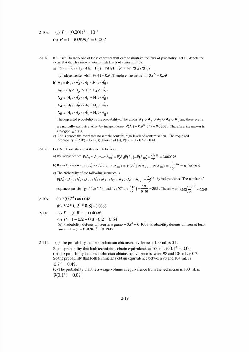
2-106. (a)62 10)001.0( −==P
(b) 002.0)999.0(1 2 =−=P
2-107. It is useful to work one of these exercises with care to illustrate the laws of probability. Let Hi denote the
event that the ith sample contains high levels of contamination.
a) P H H H H H P H P H P H P H P H( ) ( ) ( ) ( ) ( ) ( )' ' ' ' ' ' ' ' ' '1 2 3 4 5 1 2 3 4 5∩ ∩ ∩ ∩ =
by independence. Also, P H . Therefore, the answer isi( ) .' = 0 9 0 9 0 595. .=
b) A H H H H H1 1 2 3 4 5= ∩ ∩ ∩ ∩( )' ' ' '
A H H H H H2 1 2 3 4 5= ∩ ∩ ∩ ∩( )' ' ' '
A H H H H H3 1 2 3 4 5= ∩ ∩ ∩ ∩( )' ' ' '
A H H H H H4 1 2 3 4 5= ∩ ∩ ∩ ∩( )' ' ' '
A H H H H H5 1 2 3 4 5= ∩ ∩ ∩ ∩( )' ' ' '
The requested probability is the probability of the union and these eventsA A A A A1 2 3 4
∪ ∪ ∪ ∪5
are mutually exclusive. Also, by independence P A . Therefore, the answer isi( ) . ( . ) .= =0 9 01 0 06564
5(0.0656) = 0.328.
c) Let B denote the event that no sample contains high levels of contamination. The requested
probability is P(B') = 1 - P(B). From part (a), P(B') = 1 - 0.59 = 0.41.
2-108. Let A denote the event that the ith bit is a one.i
a) By independence P A A A P A P A P A( ... ) ( ) ( )... ( ) ( ) .1 2 10 1 2 10101
20 000976∩ ∩ ∩ = = =
b) By independence, P A A A P A P A P Ac( . . . ) ( ) ( ). . . ( ) ( ) .' ' ' ' '1 2 10 1 2 10
101
20 000976∩ ∩ ∩ = = =
c) The probability of the following sequence is
P A A A A A A A A A A( )' ' ' ' '1 2 3 4 5 6 7 8 9
10
101
2
∩ ∩ ∩ ∩ ∩ ∩ ∩ ∩ ∩ = ( ) , by independence. The number of
sequences consisting of five "1"'s, and five "0"'s is ( )510 10
5 5252= =
!
! !. The answer is252
1
20 246
10⎛
⎝ ⎜
⎞
⎠⎟ = .
2-109. (a) =0.0048)2.0(3 4
(b) =0.0768)8.0*2.0*4(3 3
2-110. (a) 4096.0)8.0( 4 ==P
(b) 64.02.08.02.01 =×−−=P
(c) Probability defeats all four in a game = 0.84
= 0.4096. Probability defeats all four at least
once = 1 – (1 – 0.4096)3
= 0.7942
2-111. (a) The probability that one technician obtains equivalence at 100 mL is 0.1.So the probability that both technicians obtain equivalence at 100 mL is .01.01.0 2 =(b) The probability that one technician obtains equivalence between 98 and 104 mL is 0.7.
So the probability that both technicians obtain equivalence between 98 and 104 mL is
.49.07.0 2 =(c) The probability that the average volume at equivalence from the technician is 100 mL is
.09.0)1.0(9 2 =
2-19

7/12/2019 Solution Manual Stats
http://slidepdf.com/reader/full/solution-manual-stats 25/588
2-112. (a)10
16
6
1010
10 −==P
(b) 020833.0)12
1(25.0 =×=P
2-113. Let A denote the event that a sample is produced in cavity one of the mold.
a) By independence, P A A A A A( ) ( )1 2 3 4 5
51
80 00003∩ ∩ ∩ ∩ = = .
b) Let Bi be the event that all five samples are produced in cavity i. Because the B's are mutually
exclusive, P B B B P B P B P B( ... ) ( ) ( ) ... ( )1 2 8 1 2 8∪ ∪ ∪ = + + +
From part a., P Bi( ) ( )=1
8
5 . Therefore, the answer is 81
80 000245( ) .=
c) By independence, P A A A A A( ) ( ) ( )'1 2 3 4 5
41
8
7
8∩ ∩ ∩ ∩ = . The number of sequences in
which four out of five samples are from cavity one is 5. Therefore, the answer is 51
8
7
80 001074( ) ( ) .= .
2-114. Let A denote the upper devices function. Let B denote the lower devices function.P(A) = (0.9)(0.8)(0.7) = 0.504
P(B) = (0.95)(0.95)(0.95) = 0.8574
P(A∩B) = (0.504)(0.8574) = 0.4321
Therefore, the probability that the circuit operates = P(A∪B) = P(A) +P(B) − P(A∩B) = 0.9293
2-115. [1-(0.1)(0.05)][1-(0.1)(0.05)][1-(0.2)(0.1)] = 0.9702

7/12/2019 Solution Manual Stats
http://slidepdf.com/reader/full/solution-manual-stats 26/588
Section 2-7
2-116. Because, P( A B ) P(B) = P( ) = P(A B∩ B A ) P(A),
28.05.0
)2.0(7.0
)(
)()()( ===
AP
BP B AP A BP
2-117.' '
( ) ( ) ( ) ( )( )
( ) ( ) ( ) ( ) ( )
0.4 0.80.89
0.4 0.8 0.2 0.2
P A B P B P A B P BP B A
P A P A B P B P A B P B= =
+
×= =
× + ×
2-118. Let F denote a fraudulent user and let T denote a user that originates calls from two or more
metropolitan areas in a day. Then,
003.0)9999(.01.0)0001.0(30.0
)0001.0(30.0
)'()'()()(
)()()( =
+
=
+
=
F PF T PF PF T P
F PF T PT F P
2-119. (a) P=(0.31)(0.978)+(0.27)(0.981)+(0.21)(0.965)+(0.13)(0.992)+(0.08)(0.959)
= 0.97638
(b) 207552.097638.0
)965.0)(21.0(==P
2-120. Let A denote the event that a respondent is a college graduate and let B denote the event that a
voter votes for Bush.
2-20

7/12/2019 Solution Manual Stats
http://slidepdf.com/reader/full/solution-manual-stats 27/588
%3821.39)5.0)(62.0()53.0)(38.0(
)53.0)(38.0(
)'|()'()|()(
)|()(
)(
)()|( =
+
=
+
=∩
=
A BP AP A BP AP
A BP AP
BP
B AP B AP
2-121. Let G denote a product that received a good review. Let H, M, and P denote products that were high,
moderate, and poor performers, respectively.
a)
P G P G H P H P G M P M P G P P P( ) ( ) ( ) ( ) ( ) ( ) ( )
. ( . ) . ( . ) . ( . )
.
= + +
= + +
=
0 95 0 40 0 60 0 35 0 10 0 25
0 615
b) Using the result from part a.,
P H GP G H P H
P G( )
( ) ( )
( )
. ( . )
..= = =
0 95 0 40
0 6150 618
c) P H GP G H P H
P G( ' )
( ' ) ( )
( ' )
. ( . )
..= =
−
=0 05 0 40
1 0 6150 052
2-122. a) P(D)=P(D|G)P(G)+P(D|G’)P(G’)=(.005)(.991)+(.99)(.009)=0.013865
b) P(G|D’)=P(G∩D’)/P(D’)=P(D’|G)P(G)/P(D’)=(.995)(.991)/(1-.013865)=0.9999
2-123.a) P(S) = 0.997(0.60) + 0.9995(0.27) + 0.897(0.13) = 0.9847
b) P(Ch|S) =(0.13)( 0.897)/0.9847 = 0.1184

7/12/2019 Solution Manual Stats
http://slidepdf.com/reader/full/solution-manual-stats 28/588
Section 2-8
2-124. Continuous: a, c, d, f, h, i; Discrete: b, e, and g

7/12/2019 Solution Manual Stats
http://slidepdf.com/reader/full/solution-manual-stats 29/588
Supplemental Exercises
2-125. Let B denote the event that a glass breaks.
Let L denote the event that large packaging is used.
P(B)= P(B|L)P(L) + P(B|L')P(L')
= 0.01(0.60) + 0.02(0.40) = 0.014
2-126. Let "d" denote a defective calculator and let "a" denote an acceptable calculator
a
a) { }aaadaaaad dad adaddaadd ddd S ,,,,,,,=
b) { } daadad ddaddd A ,,,=
c) { } adaadd ddaddd B ,,,=d) { }ddaddd B A ,=∩
e) { }aad dad adaadd ddaddd C B ,,,,,=∪
2-21

7/12/2019 Solution Manual Stats
http://slidepdf.com/reader/full/solution-manual-stats 30/588
2-127. Let A = excellent surface finish; B = excellent length
a) P(A) = 82/100 = 0.82
b) P(B) = 90/100 = 0.90
c) P(A') = 1 – 0.82 = 0.18
d) P(A∩B) = 80/100 = 0.80
e) P(A∪B) = 0.92f) P(A’∪B) = 0.98
2-128. a) (207+350+357-201-204-345+200)/370 = 0.9838
b) 366/370 = 0.989
c) (200+163)/370 = 363/370 = 0.981
d) (201+163)/370 = 364/370 = 0.984
2-129. If A,B,C are mutually exclusive, then P( ) = P(A) + P(B) + P(C) = 0.3 + 0.4 + 0.5 =A B C∪ ∪1.2, which greater than 1. Therefore, P(A), P(B),and P(C) cannot equal the given values.
2-130. a) 345/357 b) 5/13
2-131 (a) P(the first one selected is not ionized)=20/100=0.2
(b)P(the second is not ionized given the first one was ionized)
=20/99=0.202
(c)
P(both are ionized)
=P(the first one selected is ionized) × P(the second is ionized given the first one was ionized)
=(80/100)× (79/99)=0.638
(d)
If samples selected were replaced prior to the next selection,
P(the second is not ionized given the first one was ionized)
=20/100=0.2.
The event of the first selection and the event of the second selection are independent.
2-132. a) P(A) = 15/40
b) P(B A ) = 14/39
c) P( A ) = P(A) P(B/A) = (15/40) (14/39) = 0.135B∩
d) P( ) = 1 – P(A’ and B’) =A B∪ 25 241 0.615
40 39
⎛ ⎞⎛ ⎞− =⎜ ⎟⎜ ⎟
⎝ ⎠⎝ ⎠
A = first is local, B = second is local, C = third is local
e) P(A ∩ B ∩ C) = (15/40)(14/39)(13/38) = 0.046
f) P(A ∩ B ∩ C’) = (15/40)(14/39)(25/39) = 0.089
2-133. a) P(A) = 0.03
b) P(A') = 0.97
c) P(B|A) = 0.40
d) P(B|A') = 0.05
e) P( ) = P(A B∩ B A )P(A) = (0.40)(0.03) = 0.012
f) P( ') = P(A B∩ B A' )P(A) = (0.60)(0.03) = 0.018
g) P(B) = P(B A )P(A) + P(B A ')P(A') = (0.40)(0.03) + (0.05)(0.97) = 0.0605
2-134. Let U denote the event that the user has improperly followed installation instructions.
2-22

7/12/2019 Solution Manual Stats
http://slidepdf.com/reader/full/solution-manual-stats 31/588
Let C denote the event that the incoming call is a complaint.
Let P denote the event that the incoming call is a request to purchase more products.
Let R denote the event that the incoming call is a request for information.
a) P(U|C)P(C) = (0.75)(0.03) = 0.0225
b) P(P|R)P(R) = (0.50)(0.25) = 0.125
2-135. (a) 18143.0)002.01(1100
=−−=P
(b) 005976.0002.0)998.0( 21
3 == C P
(c) 86494.0])002.01[(1 10100 =−−=P
2-136. P( ) = 80/100, P(A) = 82/100, P(B) = 90/100.A B∩
Then, P( A ) ≠ P(A)P(B), so A and B areB∩ not independent.
2-137. Let Ai denote the event that the ith readback is successful. By independence,
P A A A P A P A P A( ) ( ) ( ) ( ) ( . ) .' ' ' ' ' '1 2 3 1 2 3
30 02 0 000008∩ ∩ = = = .
2-138.
backup main-storage
0.25 0.75
life > 5 yrslife > 5 yrs
life < 5 yrs life < 5 yrs
0.95(0.25)=0.2375 0.05(0.25)=0.0125 0.995(0.75)=0.74625 0.005(0.75)=0.00375
a) P(B) = 0.25
b) P( AB ) = 0.95
c) P( AB ') = 0.995
d) P( ) = P(A B∩ AB )P(B) = 0.95(0.25) = 0.2375
e) P( ') = P(A B∩ AB ')P(B') = 0.995(0.75) = 0.74625
f) P(A) = P( ) + P( ') = 0.95(0.25) + 0.995(0.75) = 0.98375A B∩ A B∩
g) 0.95(0.25) + 0.995(0.75) = 0.98375.
h)
769.0)75.0(005.0)25.0(05.0
)25.0(05.0
)'()''()()'(
)()'()'( =
+=
+=
BP B AP BP B AP
BP B AP A BP
2-139. (a) =∩ B A' 50
(b) B’=37(c) =∪ B A 93
2-140. a) 0.25
b) 0.75
2-141. Let Di denote the event that the primary failure mode is type i and let A denote the event that a board passes
the test.
2-23

7/12/2019 Solution Manual Stats
http://slidepdf.com/reader/full/solution-manual-stats 32/588
The sample space is S = { } .A A D A D A D A D A D, ' , ' , ' , ' , '1 2 3 4 5
2-142. a) 20/200 b) 135/200 c) 65/200
2-24
7/12/2019 Solution Manual Stats
http://slidepdf.com/reader/full/solution-manual-stats 33/588
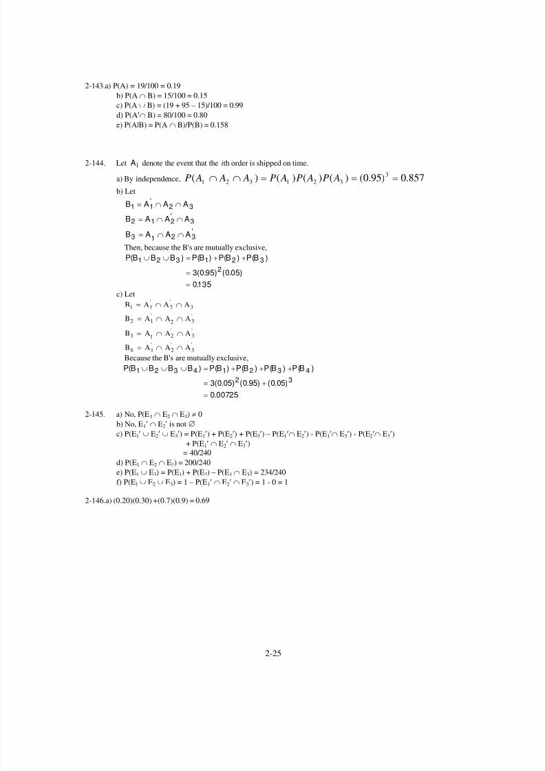
2-143.a) P(A) = 19/100 = 0.19
b) P(A ∩ B) = 15/100 = 0.15
c) P(A ∪ B) = (19 + 95 – 15)/100 = 0.99
d) P(A′∩ B) = 80/100 = 0.80
e) P(A|B) = P(A ∩ B)/P(B) = 0.158
2-144. Let A denote the event that the ith order is shipped on time.i
a) By independence, 857.0)95.0()()()()( 3
321321 ===∩∩ AP AP AP A A AP
b) Let
B A A A
B A A A
B A A A
1 1 2 3
2 1 2 3
3 1 2 3
= ∩ ∩
= ∩ ∩
= ∩ ∩
'
'
'
Then, because the B's are mutually exclusive,
P B B B P B P B P B( ) ( ) ( )
( . ) ( . )
.
1 2 3 1 2 3
23 0 95 0 05
0135
∪ ∪ = + +
=
=
( )
3= ∩ ∩
= ∩ ∩
= ∩ ∩
= ∩ ∩
' '
' '
' '
' ' '
( )
c) Let
B A A A
B A A A
B A A A
B A A A
1 1 2
2 1 2 3
3 1 2 3
4 1 2 3
Because the B's are mutually exclusive,
P B B B B P B P B P B P B( ) ( ) ( ) ( )
( . ) ( . ) ( . )
.
1 2 3 4 1 2 3 4
2 33 0 05 0 95 0 05
0 00725
∪ ∪ ∪ = + + +
= +
=
2-145. a) No, P(E1 ∩ E2 ∩ E3) ≠ 0
b) No, E1′ ∩ E2′ is not ∅
c) P(E1′ ∪ E2′ ∪ E3′) = P(E1′) + P(E2′) + P(E3′) – P(E1′∩ E2′) - P(E1′∩ E3′) - P(E2′∩ E3′)+ P(E1′ ∩ E2′ ∩ E3′)
= 40/240
d) P(E1 ∩ E2 ∩ E3) = 200/240
e) P(E1 ∪ E3) = P(E1) + P(E3) – P(E1 ∩ E3) = 234/240
f) P(E1 ∪ E2 ∪ E3) = 1 – P(E1′ ∩ E2′ ∩ E3′) = 1 - 0 = 1
2-146.a) (0.20)(0.30) +(0.7)(0.9) = 0.69
2-25

7/12/2019 Solution Manual Stats
http://slidepdf.com/reader/full/solution-manual-stats 34/588
2-147. Let Ai denote the event that the ith bolt selected is not torqued to the proper limit.
a) Then,
282.020
15
19
14
18
13
17
12
)()()()(
)()()(
1122133214
32132144321
=⎟ ⎠
⎞
⎜⎝
⎛
⎟ ⎠
⎞
⎜⎝
⎛
⎟ ⎠
⎞
⎜⎝
⎛
⎟ ⎠
⎞
⎜⎝
⎛
=
∩∩∩=
∩∩∩∩=∩∩∩
AP A AP A A AP A A A AP
A A AP A A A AP A A A AP
b) Let B denote the event that at least one of the selected bolts are not properly torqued. Thus, B' is the
event that all bolts are properly torqued. Then,
P(B) = 1 - P(B') = 115
20
14
19
13
18
12
170718−
⎛
⎝ ⎜
⎞
⎠⎟
⎛
⎝ ⎜
⎞
⎠⎟
⎛
⎝ ⎜
⎞
⎠⎟
⎛
⎝ ⎜
⎞
⎠⎟ = .
2-148. Let A,B denote the event that the first, second portion of the circuit operates. Then, P(A) =
(0.99)(0.99)+0.9-(0.99)(0.99)(0.9) = 0.998
P(B) = 0.9+0.9-(0.9)(0.9) = 0.99 and
P( ) = P(A) P(B) = (0.998) (0.99) = 0.988A B∩
2-149.A1 = by telephone, A2 = website; P(A1) = 0.92, P(A2) = 0.95;
By independence P(A1 ∪ A2) = P(A1) + P(A2) - P(A1 ∩ A2) = 0.92 + 0.95 - 0.92(0.95) = 0.996
2-150.P(Possess) = 0.95(0.99) +(0.05)(0.90) = 0.9855
2-151. Let D denote the event that a container is incorrectly filled and let H denote the event that a container is
filled under high-speed operation. Then,
a) P(D) = P(DH )P(H) + P(D H ')P(H') = 0.01(0.30) + 0.001(0.70) = 0.0037
b) 8108.00037.0
)30.0(01.0
)(
)()()( ===
DP
H P H DP D H P
2-152.a) P(E’ ∩ T’ ∩ D’) = (0.995)(0.99)(0.999) = 0.984
b) P(E ∪ D) = P(E) + P(D) – P(E ∩ D) = 0.005995
2-153.D = defective copy
a) P(D = 1) = 0778.0
73
2
74
72
75
73
73
72
74
2
75
73
73
72
74
73
75
2=
⎠
⎞⎜
⎝
⎛⎟
⎠
⎞⎜
⎝
⎛⎟
⎠
⎞⎜
⎝
⎛+
⎠
⎞⎜
⎝
⎛⎟
⎠
⎞⎜
⎝
⎛⎟
⎠
⎞⎜
⎝
⎛+
⎠
⎞⎜
⎝
⎛⎟
⎠
⎞⎜
⎝
⎛⎟
⎠
⎞⎜
⎝
⎛
b) P(D = 2) = 00108.073
1
74
2
75
73
73
1
74
73
75
2
73
73
74
1
75
2=⎟
⎠
⎞⎜⎝
⎛ ⎟
⎠
⎞⎜⎝
⎛ ⎟
⎠
⎞⎜⎝
⎛ +⎟
⎠
⎞⎜⎝
⎛ ⎟
⎠
⎞⎜⎝
⎛ ⎟
⎠
⎞⎜⎝
⎛ +⎟
⎠
⎞⎜⎝
⎛ ⎟
⎠
⎞⎜⎝
⎛ ⎟
⎠
⎞⎜⎝
⎛
c) Let A represent the event that the two items NOT inspected are not defective. Then,
P(A)=(73/75)(72/74)=0.947.
2-154. The tool fails if any component fails. Let F denote the event that the tool fails. Then, P(F') = 0 9 by
independence and P(F) = 1 - 0 9 = 0.0956
910.
910.
2-155. a) (0.3)(0.99)(0.985) + (0.7)(0.98)(0.997) = 0.9764
b) 3159.09764.01
)30.0(02485.0
)(
)1()1()1( =
−==
E P
routeProute E P E routeP
2-26

7/12/2019 Solution Manual Stats
http://slidepdf.com/reader/full/solution-manual-stats 35/588
2-156. a) By independence, 0 15 7 59 105 5. .= × −
b) Let A denote the events that the machine is idle at the time of your ith request. Using independence,i
the requested probability is
0022.0
)85.0)(15.0(5
)85.0(15.0)85.0(15.0)85.0(15.0)85.0(15.0)85.0(15.0
)(
4
44444
5432
'
1543
'
2154
'
3215
'
4321
'
54321
=
=++++=
A A A A Aor A A A A Aor A A A A Aor A A A A Aor A A A A AP
c) As in part b, the probability of 3 of the events is
0244.0
)85.0)(15.0(10
)
(
23
543
'
2
'
154
'
32
'
15
'
432
'
1
'
5432
'
154
'
3
'
21
5
'
43
'
21
'
543
'
215
'
4
'
321
'
54
'
321
'
5
'
4321
=
=
A A A A Aor A A A A Aor A A A A Aor A A A A Aor A A A A A
or A A A A Aor A A A A Aor A A A A Aor A A A A Aor A A A A AP
For the probability of at least 3, add answer parts a) and b) to the above to obtain the requested probability.
Therefore, the answer is 0.0000759 + 0.0022 + 0.0244 = 0.0267
2-157. Let A denote the event that the ith washer selected is thicker than target.i
a) 207.048
28
49
29
50
30=⎟
⎠
⎞⎜⎝
⎛ ⎟
⎠
⎞⎜⎝
⎛ ⎟
⎠
⎞⎜⎝
⎛
b) 30/48 = 0.625
c) The requested probability can be written in terms of whether or not the first and second washer selected
are thicker than the target. That is,
60.0
49
19
50
20
48
30
49
30
50
20
48
29
49
30
50
20
48
29
49
29
50
30
48
28
)()()()()()(
)()()()()()(
)()()()'(
)()()()(
)()(
'
1
'
1
'
2
'
2
'
13
'
1
'
122
'
13
11
'
2
'
213112213
'
2
'
1
'
2
'
132
'
1213
'
21
'
21321213
3
'
2
'
132
'
13
'
213213
=
⎟ ⎠
⎞⎜⎝
⎛ +⎟
⎠
⎞⎜⎝
⎛ +⎟
⎠
⎞⎜⎝
⎛ +⎟
⎠
⎞⎜⎝
⎛ =
++
+=
++
+=
=
AP A AP A A AP AP A AP A A AP
AP A AP A A AP AP A AP A A AP
A AP A A AP A AP A A AP
A AP A A AP A AP A A AP
A AorA A AorA A AorA A A AP AP
2-158. a) If n washers are selected, then the probability they are all less than the target is20
50
19
49
20 1
50 1⋅ ⋅
− +
− +...
n
n.
n probability all selected washers are less than target
1 20/50 = 0.42 (20/50)(19/49) = 0.155
3 (20/50)(19/49)(18/48) = 0.058
Therefore, the answer is n = 3
b) Then event E that one or more washers is thicker than target is the complement of the event that all are
less than target. Therefore, P(E) equals one minus the probability in part a. Therefore, n = 3.
2-27

7/12/2019 Solution Manual Stats
http://slidepdf.com/reader/full/solution-manual-stats 36/588
2-159.
547.0940
514)''()
881.0940
24668514)'()
262.0940
246)()
453.0940
24668112)()
==∩
=++=∪
==∩
=++
=∪
B APd
B APc
B APb
B APa
. e) P( AB ) =P A B
P B
( )
( )
/
/ .
∩= =
246 940
314 9400783
f) P(B A ) = P B A
P A
( )
( )
/
/ .
∩= =
246 940
358 9400 687
2-160. Let E denote a read error and let S,O,P denote skewed, off-center, and proper alignments, respectively.
Then,
a) P(E) = P(E|S) P(S) + P(E|O) P (O) + P(E|P) P(P)
= 0.01(0.10) + 0.02(0.05) + 0.001(0.85)= 0.00285
b) P(S|E) =P E S P S
P E
( ) ( )
( )
. ( . )
..= =
0 01 0 10
0 002850 351
2-161. Let A denote the event that the ith row operates. Then,
.i
P A P A P A P A( ) . , ( ) ( . )( . ) . , ( ) . , ( ) .1 2 3 40 98 0 99 0 99 0 9801 0 9801 0 98= = = = =
The probability the circuit does not operate is7'
4'3
'2
'1 1058.1)02.0)(0199.0)(0199.0)(02.0()()()()( −×== AP AP AP AP
2-162. a) (0.4)(0.1) + (0.3)(0.1) +(0.2)(0.2) + (0.4)(0.1) = 0.15
b) P(4 or more | provided info) = (0.4)(0.1)/0.15 = 0.267
2-163. (a) P=(0.93)(0.91)(0.97)(0.90)(0.98)(0.93)=0.67336
(b) P=(1-0.93)(1-0.91)(1-0.97)(1-0.90)(1-0.98)(1-0.93)=2.646×10⁻⁸
(c) P=1-(1-0.91)(1-0.97)(1-0.90)=0.99973
2-164. (a) P=(24/36)(23/35)(22/34)(21/33)(20/32)(19/31)=0.069
(b) P=1-0.069=0.931
2-165. (a) 367
(b) Number of permutations of six letters is 266. Number of ways to select one number = 10.
Number of positions among the six letters to place the one number = 7. Number of passwords =
266 × 10 × 7
(c) 265102
2-166. (a) 087.01000
20730255)( =
++++= AP
(b) 032.01000
725)( =
+=∩ B AP
(c) 20.01000
8001)( =−=∪ B AP
2-28

7/12/2019 Solution Manual Stats
http://slidepdf.com/reader/full/solution-manual-stats 37/588
(d) 113.01000
153563)'( =
++=∩ B AP
(e) 2207.01000 / )357156325(
032.0
)(
)()|( =
++++=
∩=
BP
B AP B AP
(f) 005.01000
5
==P
2-167. (a) Let A denote that a part conforms to specifications and let B denote for a part a simple
component.
For supplier 1,
P(A)=P(A|B)P(B)+ P(A|B’)P(B’)
= [(1000-2)/1000](1000/2000)+ [(1000-10)/1000](1000/2000)
= 0.994
For supplier 2,
P(A)= P(A|B)P(B)+ P(A|B’)P(B’)
= [(1600-4)/1600](1600/2000)+ [(400-6)/400](400/2000)
= 0.995
(b)
For supplier 1, P(A|B’)=0.99
For supplier 2, P(A|B’)=0.985
(c)
For supplier 1, P(A|B)=0.998
For supplier 2, P(A|B)=0.9975
(d) The unusual result is that for both a simple component and for a complex assembly, supplier 1
has a greater probability that a part conforms to specifications. However, for overall parts,
supplier 1 has a lower probability. The overall conforming probability is dependent on both the
conforming probability conditioned on the part type and the probability of each part type. Supplier
1 produces more of the compelx parts so that overall conformance from supplier 1 is lower.

7/12/2019 Solution Manual Stats
http://slidepdf.com/reader/full/solution-manual-stats 38/588
Mind Expanding Exercises
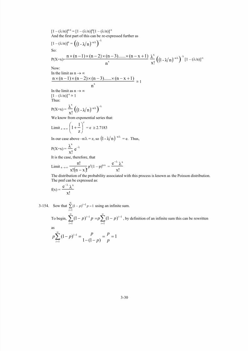
3-153. The binomial distribution
P(X=x) =( )!xn!x
!n
− px(1-p)n-x
If n is large, then the probability of the event could be expressed as λ/n, that is λ=np. Wecould re-write the probability mass function as:
P(X=x) =( )!xn!x
!n
−[λ/n]x[1 – (λ/n)]n-x
Where p = λ/n.
P(X=x)n
1)x(n3)......(n2)(n1)(nnx
+−×−×−×−×x!
λ x(1 – (λ/n))n-x
Now we can re-express:
3-29
7/12/2019 Solution Manual Stats
http://slidepdf.com/reader/full/solution-manual-stats 39/588
[1 – (λ/n)]n-x = [1 – (λ/n)]n[1 – (λ/n)]-x And the first part of this can be re-expressed further as
[1 – (λ/n)]n = ( )( )nλ -1n/λ
λ −
−
So:
P(X=x)= n
1)x(n3)......(n2)(n1)(nnx
+−×−×−×−×
x!
λ x
( )( )nλ -1n/λ
λ −
−
[1 – (λ/n)]-x
Now:
In the limit as n → ∞
n
1)x(n3)......(n2)(n1)(nnx
+−×−×−×−× ≅ 1
In the limit as n → ∞
[1 – (λ/n)]-x ≅ 1Thus:
P(X=x) =x!
λ x
( )( )nλ -1n/λ
λ −
−
We know from exponential series that:
Limit z → ∞ ⎟ ⎠
⎞⎜⎝
⎛ +
z
11
z
= e ≅ 2.7183
In our case above –n/λ = z, so ( )nλ -1n/λ −
= e. Thus,
P(X=x) =x!
λ x
eλ −
It is the case, therefore, that
Limit n → ∞ ( )!xn!x
!n
− px(1 – p)n-x =
!x
e xλ
λ−
The distribution of the probability associated with this process is known as the Poisson distribution.
The pmf can be expressed as:
f(x) =!x
e xλ
λ−
3-154. Sow that using an infinite sum.∑∞
=
− =−1
1 1)1(i
i p p
To begin, , by definition of an infinite sum this can be rewritten
as
∑∑∞
=
−∞
=
− −=−1
1
1
1 )1()1(i
i
i
i p p p p
1
)1(1
)1(
1
1 ==−−
=−∑∞
=
−
p
p
p
p p p
i
i
3-30

7/12/2019 Solution Manual Stats
http://slidepdf.com/reader/full/solution-manual-stats 40/588
3-155.
[ ]
1
1 1
2 2
2 2
2
( ) [( ( 1) ... ]( 1)
( 1) ( 1)
2 2( 1) ( 1)
( ) ( )( 1)
2 2( 1) ( 1)
( )
2
( 1)(( )
( )1
b a
i i
b bb
b a
i a i ai a
E X a a b b a
b b a ai i
b a b a
b a b a b a b a
b a b a
b a
b a b ai b a ii
V X b a
−
= =
+
= ==
= + + + + − +
⎡ ⎤ + −⎡ ⎤− −⎢ ⎥ ⎢ ⎥⎣ ⎦ ⎣ ⎦= =− + − +
⎡ ⎤− + + + − +⎡ ⎤⎢ ⎥ ⎢ ⎥⎣ ⎦ ⎣ ⎦= =
− + − +
+=
− + +− + +−
= =+ −
∑ ∑
∑ ∑∑2
2
2
)
4
1
( 1)(2 1) ( 1) (2 1) ( 1) ( 1) ( 1)( )( )6 6 2 4
1
( 1) 1
12
b a
b b b a a a b b a a b a b ab a
b a
b a
⎡ ⎤⎢ ⎥⎣ ⎦
+ −
+ + − − + − − − + +⎡ ⎤− − + +⎢ ⎥⎣ ⎦=
− +
− + −=
3-156. Let X denote the number of nonconforming products in the sample. Then, X is approximately binomial with
p = 0.01 and n is to be determined.
If , then90.0)1( ≥≥ X P 10.0)0( ≤= X P .
Now, P(X = 0) = ( ) nnn p p p )1()1(0
0 −=− . Consequently, , and( ) .1 0− ≤p n 10
11.229)1ln(
10.0ln =−
≤ p
n . Therefore, n = 230 is required
3-157. If the lot size is small, 10% of the lot might be insufficient to detect nonconforming product. For example, if
the lot size is 10, then a sample of size one has a probability of only 0.2 of detecting a nonconforming
product in a lot that is 20% nonconforming.
If the lot size is large, 10% of the lot might be a larger sample size than is practical or necessary. For
example, if the lot size is 5000, then a sample of 500 is required. Furthermore, the binomialapproximation to the hypergeometric distribution can be used to show the following. If 5% of the lot of size
5000 is nonconforming, then the probability of zero nonconforming product in the sample is approximately
. Using a sample of 100, the same probability is still only 0.0059. The sample of size 500 might7 10 12× −
be much larger than is needed.
3-31

7/12/2019 Solution Manual Stats
http://slidepdf.com/reader/full/solution-manual-stats 41/588
3-158. Let X denote the number of panels with flaws. Then, X is a binomial random variable with n =100 and p is
the probability of one or more flaws in a panel. That is, p = = 0.095.1.01 −− e
( ) ( ) ( )
( ) ( )
034.0
)1()1(
)1()1()1(
)4()3()2()1()0()4()5(
9641004
9731003
9821002
9911001
10001000
=
−+−+
−+−+−=
=+=+=+=+==≤=<
p p p p
p p p p p p
X P X P X P X P X P X P X P
3-159. Let X denote the number of rolls produced.
Revenue at each demand
0 1000 2000 3000
0 1000≤ ≤x 0.05x 0.3x 0.3x 0.3x
mean profit = 0.05x(0.3) + 0.3x(0.7) - 0.1x
1000 2000≤ ≤x 0.05x 0.3(1000) +0.05(x-1000)
0.3x 0.3x
mean profit = 0.05x(0.3) + [0.3(1000) + 0.05(x-1000)](0.2) + 0.3x(0.5) - 0.1x
2000 3000≤ ≤x 0.05x 0.3(1000) +
0.05(x-1000)
0.3(2000) +
0.05(x-2000)
0.3x
mean profit = 0.05x(0.3) + [0.3(1000)+0.05(x-1000)](0.2) + [0.3(2000) + 0.05(x-2000)](0.3) + 0.3x(0.2) - 0.1x
3000 ≤ x 0.05x 0.3(1000) +
0.05(x-1000)
0.3(2000) +
0.05(x-2000)
0.3(3000)+
0.05(x-3000)
mean profit = 0.05x(0.3) + [0.3(1000)+0.05(x-1000)](0.2) + [0.3(2000)+0.05(x-2000)]0.3 + [0.3(3000)+0.05(x-
3000)]0.2 - 0.1x
Profit Max. profit
0 1000≤ ≤x 0.125 x $ 125 at x = 1000
1000 2000≤ ≤x 0.075 x + 50 $ 200 at x = 2000
2000 3000≤ ≤x 200 $200 at x = 3000
3000 ≤ x -0.05 x + 350 $200 at x = 3000
The bakery can make anywhere from 2000 to 3000 and earn the same profit.
3-160.Let X denote the number of acceptable components. Then, X has a binomial distribution with p = 0.98 and
n is to be determined such that P X .( ) .≥ ≥100 0 95
n P X( )≥ 100
102 0.666
103 0.848
104 0.942
105 0.981
Therefore, 105 components are needed.
3-32

7/12/2019 Solution Manual Stats
http://slidepdf.com/reader/full/solution-manual-stats 42/588
CHAPTER 3
Section 3-1
3-1. The range of X is { } 1000,...,2,1,0
3-2. The range of X is { } 0 12 50, , ,...,
3-3. The range of X is { } 0 1 2 99999, , ,...,
3-4. The range of X is { } 0 1 2 3 4 5, , , , ,
3-5. The range of X is { . Because 490 parts are conforming, a nonconforming part must be
selected in 491 selections.
}
}
491,...,2,1
3-6. The range of X is { . Although the range actually obtained from lots typically might not
exceed 10%.
0 12 100, , ,...,
3-7. The range of X is conveniently modeled as all nonnegative integers. That is, the range of X is{ }0 12, , ,...
3-8. The range of X is conveniently modeled as all nonnegative integers. That is, the range of X is
{ }0 12, , ,...
3-9. The range of X is { } 15,...,2,1,0
3-10. The possible totals for two orders are 1/8 + 1/8 = 1/4, 1/8 + 1/4 = 3/8, 1/8 + 3/8 = 1/2, 1/4 + 1/4 = 1/2,
1/4 + 3/8 = 5/8, 3/8 + 3/8 = 6/8.
Therefore the range of X is1
4
3
8
1
2
5
8
6
8, , , ,
⎧⎨⎩
⎫⎬⎭
3-11. The range of X is }10000,,2,1,0{ …
3-12.The range of X is {100, 101, …, 150}
3-13.The range of X is {0,1,2,…, 40000)

7/12/2019 Solution Manual Stats
http://slidepdf.com/reader/full/solution-manual-stats 43/588
Section 3-2
3-14.
6/1)3(
6/1)2(
3/1)5.1()5.1(
3/16/16/1)0()0(
=
=
===
=+===
X
X
X
X
f
f
X P f
X P f
a) P( X = 1.5) = 1/3
b) P(0.5< X < 2.7) = P( X = 1.5) +P( X = 2) = 1/3 + 1/6 = 1/2
c) P( X > 3) = 0
d) (0 2) ( 0) ( 1.5) 1/ 3 1/ 3 2 / 3P X P X P X ≤ < = = + = = + =e) P( X = 0 or X = 2) = 1/3 + 1/6 = 1/2
3-15. All probabilities are greater than or equal to zero and sum to one.
3-1

7/12/2019 Solution Manual Stats
http://slidepdf.com/reader/full/solution-manual-stats 44/588
a) P(X ≤ 2)=1/8 + 2/8 + 2/8 + 2/8 + 1/8 = 1
b) P(X > - 2) = 2/8 + 2/8 + 2/8 + 1/8 = 7/8
c) P(-1 ≤ X ≤ 1) = 2/8 + 2/8 + 2/8 =6/8 = 3/4
d) P(X ≤ -1 or X=2) = 1/8 + 2/8 +1/8 = 4/8 =1/2
3-16. All probabilities are greater than or equal to zero and sum to one.
a) P(X≤ 1)=P(X=1)=0.5714 b) P(X>1)= 1-P(X=1)=1-0.5714=0.4286
c) P(2<X<6)=P(X=3)=0.1429
d) P(X≤1 or X>1)= P(X=1)+ P(X=2)+P(X=3)=1
3-17. Probabilities are nonnegative and sum to one.
a) P(X = 4) = 9/25
b) P(X ≤ 1) = 1/25 + 3/25 = 4/25
c) P(2 ≤ X < 4) = 5/25 + 7/25 = 12/25
d) P(X > −10) = 1
3-18. Probabilities are nonnegative and sum to one.
a) P(X = 2) = 3/4(1/4)2 = 3/64
b) P(X ≤ 2) = 3/4[1+1/4+(1/4)2] = 63/64
c) P(X > 2) = 1 − P(X ≤ 2) = 1/64d) P(X ≥ 1) = 1 − P(X ≤ 0) = 1 − (3/4) = 1/4
3-19. X = number of successful surgeries.
P(X=0)=0.1(0.33)=0.033
P(X=1)=0.9(0.33)+0.1(0.67)=0.364
P(X=2)=0.9(0.67)=0.603
3-20. P(X = 0) = 0.023
= 8 x 10⁻⁶
P(X = 1) = 3[0.98(0.02)(0.02)]=0.0012
P(X = 2) = 3[0.98(0.98)(0.02)]=0.0576
P(X = 3) = 0.983 = 0.9412
3-21. X = number of wafers that pass
P(X=0) = (0.2)3 = 0.008P(X=1) = 3(0.2)2(0.8) = 0.096
P(X=2) = 3(0.2)(0.8)2 = 0.384
P(X=3) = (0.8)3 = 0.512
3-22. X: the number of computers that vote for a left roll when a right roll is appropriate.
p=0.0001.
P(X=0)=(1-p)4=0.99994=0.9996
P(X=1)=4*(1-p)3 p=4*0.999930.0001=0.0003999
P(X=2)=C42(1-p)2 p2=5.999*10-8
P(X=3)=C43(1-p)1 p3=3.9996*10-12
P(X=4)=C40(1-p)0 p4=1*10-16
3-23. P(X = 50 million) = 0.5, P(X = 25 million) = 0.3, P(X = 10 million) = 0.2
3-24. P(X = 10 million) = 0.3, P(X = 5 million) = 0.6, P(X = 1 million) = 0.1
3-25. P(X = 15 million) = 0.6, P(X = 5 million) = 0.3, P(X = -0.5 million) = 0.1
3-26. X = number of components that meet specifications
P(X=0) = (0.05)(0.02) = 0.001
P(X=1) = (0.05)(0.98) + (0.95)(0.02) = 0.068
P(X=2) = (0.95)(0.98) = 0.931
3-2

7/12/2019 Solution Manual Stats
http://slidepdf.com/reader/full/solution-manual-stats 45/588
3-27. X = number of components that meet specifications
P(X=0) = (0.05)(0.02)(0.01) = 0.00001
P(X=1) = (0.95)(0.02)(0.01) + (0.05)(0.98)(0.01)+(0.05)(0.02)(0.99) = 0.00167
P(X=2) = (0.95)(0.98)(0.01) + (0.95)(0.02)(0.99) + (0.05)(0.98)(0.99) = 0.07663
P(X=3) = (0.95)(0.98)(0.99) = 0.92169

7/12/2019 Solution Manual Stats
http://slidepdf.com/reader/full/solution-manual-stats 46/588
Section 3-3
3-28. where
⎪⎪⎪
⎭
⎪⎪⎪
⎬
⎫
⎪⎪⎪
⎩
⎪⎪⎪
⎨
⎧
≤
<≤
<≤
<≤
<
=
x
x
x
x
x
xF
31
326/5
25.13/2
5.103/1
0,0
)(
6/1)3(
6/1)2(
3/1)5.1()5.1(
3/16/16/1)0()0(
=
=
===
=+===
X
X
X
X
f
f
X P f
X P f
3-29.
where
⎪⎪⎪⎪
⎭
⎪⎪⎪⎪
⎬
⎫
⎪⎪⎪⎪
⎩
⎪⎪⎪⎪
⎨
⎧
≤
<≤
<≤
<≤−
−<≤−−<
=
x
x
x
x
x
x
xF
21
218/7
108/5
018/3
128/1
2,0
)(
8/1)2(
8/2)1(
8/2)0(
8/2)1(
8/1)2(
=
=
=
=−
=−
X
X
X
X
X
f
f
f
f
f
a) P(X ≤ 1.25) = 7/8
b) P(X ≤ 2.2) = 1
c) P(-1.1 < X ≤ 1) = 7/8 − 1/8 = 3/4
d) P(X > 0) = 1 − P(X ≤ 0) = 1 − 5/8 = 3/8
3-30. where
⎪⎪⎪⎪
⎭
⎪⎪⎪⎪
⎬
⎫
⎪⎪⎪⎪
⎩
⎪⎪⎪⎪
⎨
⎧
≤
<≤
<≤
<≤
<≤
<
=
x
x
x
x
x
x
xF
41
4325/16
3225/9
2125/4
1025/1
0,0
)(
25/9)4(
25/7)3(
25/5)2(
25/3)1(
25/1)0(
=
=
=
=
=
X
X
X
X
X
f
f
f
f
f
a) P(X < 1.5) = 4/25
b) P(X ≤ 3) = 16/25
c) P(X > 2) = 1 − P(X ≤ 2) = 1 − 9/25 = 16/25
d) P(1 < X ≤ 2) = P(X ≤ 2) − P(X ≤ 1) = 9/25 − 4/25 = 5/25 = 1/5
3-31.
3-3

7/12/2019 Solution Manual Stats
http://slidepdf.com/reader/full/solution-manual-stats 47/588
⎪
⎪⎪
⎭
⎪⎪⎪
⎬
⎫
⎪
⎪⎪
⎩
⎪⎪⎪
⎨
⎧
≤
<≤
<≤
<≤
<
=
x
x
x
x
x
xF
3,1
32,488.0
21,104.0
10,008.0
0,0
)(
where
,512.0)8.0()3(
,384.0)8.0)(8.0)(2.0(3)2(
,096.0)8.0)(2.0)(2.0(3)1(
,008.02.0)0(
.
3
3
==
==
==
==
f
f
f
f
3-32.
0, 00.9996, 0 1
( ) 0.9999, 1 3
0.99999, 3 4
1, 4
x x
F x x
x
x
<⎧ ⎫⎪ ⎪≤ <⎪ ⎪⎪ ⎪
= ≤ <⎨ ⎬⎪ ⎪≤ <⎪ ⎪
≤⎪ ⎪⎩ ⎭
where
4
3
8
12
16
.
(0) 0.9999 0.9996,
(1) 4(0.9999 )(0.0001) 0.0003999,
(2) 5.999 *10 ,
(3) 3.9996*10 ,
(4) 1*10
f
f
f
f
f
−
−
−
= =
= =
=
=
=
3-33.
⎪⎪
⎭
⎪⎪
⎬
⎫
⎪⎪
⎩
⎪⎪
⎨
⎧
≤
<≤
<≤
<
=
x
x
x
x
xF
50,1
5025,5.0
2510,2.0
10,0
)(
where P(X = 50 million) = 0.5, P(X = 25 million) = 0.3, P(X = 10 million) = 0.2
3-4

7/12/2019 Solution Manual Stats
http://slidepdf.com/reader/full/solution-manual-stats 48/588
3-34.
⎪
⎪
⎭
⎪⎪
⎬
⎫
⎪
⎪
⎩
⎪⎪
⎨
⎧
≤
<≤
<≤
<
=
x
x
x
x
xF
10,1
105,7.0
51,1.0
1,0
)(
where P(X = 10 million) = 0.3, P(X = 5 million) = 0.6, P(X = 1 million) = 0.1
3-35. The sum of the probabilities is 1 and all probabilities are greater than or equal to zero;
pmf: f (1) = 0.5, f (3) = 0.5
a) P(X ≤ 3) = 1
b) P(X ≤ 2) = 0.5
c) P(1 ≤ X ≤ 2) = P(X=1) = 0.5
d) P(X>2) = 1 − P(X≤2) = 0.5
3-36. The sum of the probabilities is 1 and all probabilities are greater than or equal to zero;
pmf: f(1) = 0.7, f(4) = 0.2, f(7) = 0.1
a) P(X ≤ 4) = 0.9
b) P(X > 7) = 0
c) P(X ≤ 5) = 0.9
d) P(X>4) = 0.1
e) P(X≤2) = 0.7
3-37. The sum of the probabilities is 1 and all probabilities are greater than or equal to zero;
pmf: f(-10) = 0.25, f(30) = 0.5, f(50) = 0.25
a) P(X≤50) = 1
b) P(X≤40) = 0.75
c) P(40 ≤ X ≤ 60) = P(X=50)=0.25
d) P(X<0) = 0.25
e) P(0≤X<10) = 0
f) P(−10<X<10) = 0
3-5

7/12/2019 Solution Manual Stats
http://slidepdf.com/reader/full/solution-manual-stats 49/588
3-38. The sum of the probabilities is 1 and all probabilities are greater than or equal to zero;
pmf: f1/8) = 0.2, f(1/4) = 0.7, f(3/8) = 0.1
a) P(X≤1/18) = 0
b) P(X≤1/4) = 0.9
c) P(X≤5/16) = 0.9
d) P(X>1/4) = 0.1
e) P(X≤1/2) = 1

7/12/2019 Solution Manual Stats
http://slidepdf.com/reader/full/solution-manual-stats 50/588
Section 3-4
3-39. Mean and Variance
2)2.0(4)2.0(3)2.0(2)2.0(1)2.0(0
)4(4)3(3)2(2)1(1)0(0)(
=++++=
++++== f f f f f X E μ
22)2.0(16)2.0(9)2.0(4)2.0(1)2.0(0
)4(4)3(3)2(2)1(1)0(0)(
2
222222
=−++++=
−++++= μ f f f f f X V
3- 40. Mean and Variance for random variable in exercise 3-14
333.1)6/1(3)6/1(2)3/1(5.1)3/1(0
)3(3)2(2)5.1(5.1)0(0)(
=+++=
+++== f f f f X E μ
139.1333.1)6/1(9)6/1(4)3/1(25.2)3/1(0
)3(3)2(2)1(5.1)0(0)(
2
22222
=−+++=
−+++= μ f f f f X V
3-41. Determine E(X) and V(X) for random variable in exercise 3-15
.0)8/1(2)8/2(1)8/2(0)8/2(1)8/1(2
)2(2)1(1)0(0)1(1)2(2)(
=+++−−=
+++−−−−== f f f f f X E μ
5.10)8/1(4)8/2(1)8/2(0)8/2(1)8/1(4
)2(2)1(1)0(0)1(1)2(2)(
2
222222
=−++++=
−+++−−−−= μ f f f f f X V
3-42. Determine E(X) and V(X) for random variable in exercise 3-16
( ) 1 (1) 2 (2) 3 (3)
1(0.5714286) 2(0.2857143) 3(0.1428571)
1.571429
E X f f f μ = = + +
= + +
=
2 2 2( ) 1 (1) 2 (2) 3 (3)
1.428571
V X f f f 2
μ = + + + −
=
3-43. Mean and variance for exercise 3-17
8.2)36.0(4)28.0(3)2.0(2)12.0(1)04.0(0
)4(4)3(3)2(2)1(1)0(0)(
=++++=
++++== f f f f f X E μ
36.18.2)36.0(16)28.0(9)2.0(4)12.0(1)04.0(0
)4(4)3(3)2(2)1(1)0(0)(
2
222222
=−++++=
−++++= μ f f f f f X V
3-6

7/12/2019 Solution Manual Stats
http://slidepdf.com/reader/full/solution-manual-stats 51/588
3-44. Mean and variance for exercise 3-18
3
1
4
1
4
3
4
1
4
3)(
10
=⎟ ⎠
⎞⎜⎝
⎛ =⎟
⎠
⎞⎜⎝
⎛ = ∑∑
∞
=
∞
= x
x
x
x
x x X E
The result uses a formula for the sum of an infinite series. The formula can be derived from the fact that the
series to sum is the derivative of a
aaah x
x
−== ∑∞
= 1)(
1
with respect to a.
For the variance, another formula can be derived from the second derivative of h(a) with respect to a.
Calculate from this formula
9
5
4
1
4
3
4
1
4
3)(
1
2
0
22 =⎟ ⎠
⎞⎜⎝
⎛ =⎟
⎠
⎞⎜⎝
⎛ = ∑∑
∞
=
∞
= x
x
x
x
x x X E
Then [ ]9
4
9
1
9
5)()()(
22 =−=−= X E X E X V
3-45. Mean and variance for random variable in exercise 3-19
( ) 0 (0) 1 (1) 2 (2)0(0.033) 1(0.364) 2(0.603)
1.57
E X f f f μ = = + += + +
=
2 2 2
2
( ) 0 (0) 1 (1) 2 (2)
0(0.033) 1(0.364) 4(0.603) 1.57
0.3111
V X f f f 2
μ = + + −
= + + −
=
3-46. Mean and variance for exercise 3-20
6
( ) 0 (0) 1 (1) 2 (2) 3 (3)
0(8 10 ) 1(0.0012) 2(0.0576) 3(0.9412)
2.940008
E X f f f f μ
−
= = + + +
= × + + +
=
2 2 2 2( ) 0 (0) 1 (1) 2 (2) 3 (3)
0.05876096
V X f f f f 2μ = + + + −
=
3-47. Determine x where range is [0,1,2,3,x] and mean is 6.
24
2.08.4
2.02.16
)2.0()2.0(3)2.0(2)2.0(1)2.0(06
)()3(3)2(2)1(1)0(06)(
=
=
+=
++++=
++++===
x
x
x
x
x xf f f f f X E μ
3-7

7/12/2019 Solution Manual Stats
http://slidepdf.com/reader/full/solution-manual-stats 52/588
3-48. (a) F(0)=0.17
Nickel Charge: X CDF
0 0.17
2 0.17+0.35=0.52
3 0.17+0.35+0.33=0.854 0.17+0.35+0.33+0.15=1
(b)E(X) = 0*0.17+2*0.35+3*0.33+4*0.15=2.29
V(X) =
42
1
( )( )i i
i
f x x μ
=
−∑ = 1.5259
3-49. X = number of computers that vote for a left roll when a right roll is appropriate.
µ = E(X)=0*f(0)+1*f(1)+2*f(2)+3*f(3)+4*f(4)
= 0+0.0003999+2*5.999*10-8+3*3.9996*10-12+4*1*10-16= 0.0004
V(X)=
5
2
1
( )( )i i
i
f x x μ
=
−∑ = 0.00039996
3-50. µ=E(X)=350*0.06+450*0.1+550*0.47+650*0.37=565
V(X)= =6875∑=
−4
1
2))((i
i x x f μ
σ= )( X V =82.92
3-51. (a)
Transaction Frequency Selects: X f(X)
New order 43 23 0.43
Payment 44 4.2 0.44
Order status 4 11.4 0.04
Delivery 5 130 0.05
Stock level 4 0 0.04
total 100
µ =
E(X) = 23*0.43+4.2*0.44+11.4*0.04+130*0.05+0*0.04 =18.694
V(X) = = 735.964∑=
−5
1
2))((i
i x x f μ 1287.27)( == X V σ
(b)
Transaction Frequency All operation: X f(X) New order 43 23+11+12=46 0.43
Payment 44 4.2+3+1+0.6=8.8 0.44
Order status 4 11.4+0.6=12 0.04
Delivery 5 130+120+10=260 0.05
Stock level 4 0+1=1 0.04
total 100
µ = E(X) = 46*0.43+8.8*0.44+12*0.04+260*0.05+1*0.04=37.172
3-8

7/12/2019 Solution Manual Stats
http://slidepdf.com/reader/full/solution-manual-stats 53/588
V(X) = =2947.996∑=
−5
1
2))((i
i x x f μ 2955.54)( == X V σ

7/12/2019 Solution Manual Stats
http://slidepdf.com/reader/full/solution-manual-stats 54/588
Section 3-5
3-52. E(X) = (0+100)/2 = 50, V(X) = [(100-0+1)2-1]/12 = 850
3-53. E(X) = (3+1)/2 = 2, V(X) = [(3-1+1)2 -1]/12 = 0.667
3-54. X=(1/100)Y, Y = 15, 16, 17, 18, 19.
E(X) = (1/100) E(Y) = 17.02
1915
100
1=⎟
⎠
⎞⎜⎝
⎛ +mm
0002.0
12
1)11519(
100
1)(
22
=⎥
⎦
⎤⎢
⎣
⎡ −+−⎟
⎠
⎞⎜
⎝
⎛ = X V mm2
3-55. 33
14
3
13
3
12)( =⎟
⎠
⎞⎜⎝
⎛ +⎟
⎠
⎞⎜⎝
⎛ +⎟
⎠
⎞⎜⎝
⎛ = X E
in 100 codes the expected number of letters is 300
( ) ( ) ( ) ( )3
23
3
14
3
13
3
12)(
2222 =−⎟ ⎠
⎞⎜⎝
⎛ +⎟
⎠
⎞⎜⎝
⎛ +⎟
⎠
⎞⎜⎝
⎛ = X V
in 100 codes the variance is 6666.67
3-56. X = 590 + 0.1Y, Y = 0, 1, 2, ..., 9
E(X) = 45.5902
901.0590 =⎟ ⎠ ⎞⎜
⎝ ⎛ ++ mm
0825.012
1)109()1.0()(
22 =⎥
⎦
⎤⎢⎣
⎡ −+−= X V mm2
3-57. a = 675, b = 700
(a) µ = E(X) = (a+b)/2= 687.5
V(X) = [(b – a +1)2
– 1]/12= 56.25
(b) a = 75, b = 100
µ = E(X) = (a+b)/2 = 87.5
V(X) = [(b – a + 1)2 – 1]/12= 56.25
The range of values is the same, so the mean shifts by the difference in the two minimums (or
maximums) whereas the variance does not change.
3-58. X is a discrete random variable. X is discrete because it is the number of fields out of 28 that has an error.
However, X is not uniform because P(X=0) ≠ P(X=1).
3-59. The range of Y is 0, 5, 10, ..., 45, E(X) = (0+9)/2 = 4.5
E(Y) = 0(1/10)+5(1/10)+...+45(1/10)
= 5[0(0.1) +1(0.1)+ ... +9(0.1)]
= 5E(X)
= 5(4.5)
= 22.5
V(X) = 8.25, V(Y) = 52(8.25) = 206.25, σY = 14.36
3-9

7/12/2019 Solution Manual Stats
http://slidepdf.com/reader/full/solution-manual-stats 55/588
3-60. ,∑∑ === x x
X cE x xf c xcxf cX E )()()()(
∑∑ =−=−= x x
X cV x f xc x f ccxcX V )()()()()()( 222μ μ

7/12/2019 Solution Manual Stats
http://slidepdf.com/reader/full/solution-manual-stats 56/588
Section 3-7
3-81 . a) 5.05.0)5.01()1( 0 =−== X P
b) 0625.05.05.0)5.01()4( 43 ==−== X P
c) 0039.05.05.0)5.01()8( 87 ==−== X P
d) 5.0)5.01(5.0)5.01()2()1()2( 10 −+−==+==≤ X P X P X P
75.05.05.02 =+=
e.) 25.075.01)2(1)2( =−=≤−=> X P X P
3-82. E(X) = 2.5 = 1/p giving p = 0.4
a) 4.04.0)4.01()1( 0 =−== X P
b) 0864.04.0)4.01()4( 3 =−== X P
c) 05184.05.0)5.01()5( 4 =−== X P
d) )3()2()1()3( =+=+==≤ X P X P X P X P
7840.04.0)4.01(4.0)4.01(4.0)4.01( 210 =−+−+−=e) 2160.07840.01)3(1)3( =−=≤−=> X P X P
3-83. Let X denote the number of trials to obtain the first success.
a) E(X) = 1/0.2 = 5
b) Because of the lack of memory property, the expected value is still 5.
3-84. a) E(X) = 4/0.2 = 20
b) P(X=20) = 0436.02.0)80.0(3
19416 =⎟⎟
⎠
⎞⎜⎜⎝
⎛
3-15

7/12/2019 Solution Manual Stats
http://slidepdf.com/reader/full/solution-manual-stats 57/588
c) P(X=19) = 0459.02.0)80.0(3
18415 =⎟⎟
⎠
⎞⎜⎜⎝
⎛
d) P(X=21) = 0411.02.0)80.0(3
20417 =⎟⎟
⎠
⎞⎜⎜⎝
⎛
e) The most likely value for X should be near μX. By trying several cases, the most likely value is x = 19.
3-85. Let X denote the number of trials to obtain the first successful alignment. Then X is a geometric random
variable with p = 0.8
a) 0064.08.02.08.0)8.01()4( 33 ==−== X P
b) )4()3()2()1()4( =+=+=+==≤ X P X P X P X P X P
8.0)8.01(8.0)8.01(8.0)8.01(8.0)8.01( 3210 −+−+−+−=
9984.08.02.0)8.0(2.0)8.0(2.08.0 32 =+++=c) )]3()2()1([1)3(1)4( =+=+=−=≤−=≥ X P X P X P X P X P
]8.0)8.01(8.0)8.01(8.0)8.01[(1 210 −+−+−−=
008.0992.01)]8.0(2.0)8.0(2.08.0[1
2
=−=++−=
3-86. Let X denote the number of people who carry the gene. Then X is a negative binomial random variable with
r=2 and p = 0.1
a) )]3()2([1)4(1)4( =+=−=<−=≥ X P X P X P X P
972.0)018.001.0(11.0)1.01(1
21.0)1.01(
1
11 2120 =+−=⎥
⎦
⎤⎢⎣
⎡−⎟⎟
⎠
⎞⎜⎜⎝
⎛ +−⎟⎟
⎠
⎞⎜⎜⎝
⎛ −=
b) 201.0/2/)( === pr X E
3-87. Let X denote the number of calls needed to obtain a connection. Then, X is a geometric random variable
with p = 0.02.
a) 0167.002.098.002.0)02.01()10( 99 ==−== X Pb) )]5()4()3()2()1([1)4(1)5( =+=+=+=+=−=≤−=> X P X P X P X P X P X P X P
)]02.0(98.0)02.0(98.0)02.0(98.0)02.0(98.0)02.0(98.002.0[1 4332 +++++−=9039.00961.01 =−=
May also use the fact that P(X > 5) is the probability of no connections in 5 trials. That is,
9039.098.002.00
5)5( 50 =⎟⎟
⎠
⎞⎜⎜⎝
⎛ => X P
c) E(X) = 1/0.02 = 50
3-88. X: # of opponents until the player is defeated.
p=0.8, the probability of the opponent defeating the player.
(a) f(x) = (1 – p)x – 1 p = 0.8(x – 1)*0.2
(b) P(X>2) = 1 – P(X=1) – P(X=2) = 0.64
(c) µ = E(X) = 1/p = 5
(d) P(X≥4) = 1-P(X=1)-P(X=2)-P(X=3) = 0.512
(e) The probability that a player contests four or more opponents is obtained in part (d), which is
po = 0.512.
Let Y represent the number of game plays until a player contests four or more opponents.
Then, f(y) = (1-po)y-1 po.
3-16

7/12/2019 Solution Manual Stats
http://slidepdf.com/reader/full/solution-manual-stats 58/588
µY = E(Y) = 1/po = 1.95
3-89. p=0.13
(a) P(X=1) = (1-0.13)1-1*0.13=0.13.
(b) P(X=3)=(1-0.13)3-1*0.13 =0.098
(c) µ=E(X)= 1/p=7.69≈
8
3-90. X: # number of attempts before the hacker selects a user password.
(a) p=9900/366=0.0000045
µ=E(X) = 1/p= 219877
V(X)= (1-p)/p2 = 4.938*1010
σ= )( X V =222222
(b) p=100/363=0.00214
µ=E(X) = 1/p= 467
V(X)= (1-p)/p2 = 217892.39
σ= )( X V =466.78
Based on the answers to (a) and (b) above, it is clearly more secure to use a 6 character password.
3-91 . p = 0.005 , r = 8
a.)198 1091.3005.0)8( −=== x X P
b). 200005.0
1)( === X E μ days
c) Mean number of days until all 8 computers fail. Now we use p=3.91x10⁻¹⁹
18
911056.2
1091.3
1)( x
xY E ===
−μ days or 7.01 x10
15years
3-92. Let Y denote the number of samples needed to exceed 1 in Exercise 3-66. Then Y has a geometric
distribution with p = 0.0169.
a) P(Y = 10) = (1 − 0.0169)9(0.0169) = 0.0145
b) Y is a geometric random variable with p = 0.1897 from Exercise 3-66.
P(Y = 10) = (1 − 0.1897)9(0.1897) = 0.0286
c) E(Y) = 1/0.1897 = 5.27
3-93. Let X denote the number of transactions until all computers have failed. Then, X is negative binomial
random variable with p = 10-8 and r = 3.
a) E(X) = 3 x 10⁸
b) V(X) = [3(1−10-80]/(10-16) = 3.0 x 10¹⁶
3-94. (a) p6=0.6, p=0.918
(b) 0.6*p
2
=0.4, p=0.816
3-95 . Negative binomial random variable: f(x; p, r) = .r r x
p pr
x −−⎟⎟ ⎠
⎞⎜⎜⎝
⎛ −
−)1(
1
1
When r = 1, this reduces to f(x; p, r) = (1− p)x-1 p, which is the pdf of a geometric random variable.
Also, E(X) = r/p and V(X) = [r(1− p)]/p2
reduce to E(X) = 1/p and V(X) = (1− p)/p2, respectively.
3-17

7/12/2019 Solution Manual Stats
http://slidepdf.com/reader/full/solution-manual-stats 59/588
3-96. Let X denote a geometric random variable with parameter p. Let q = 1-p.
1 1
21 1
1 1( ) (1 )
x x
x x
E X x p p p xq p p p
∞ ∞− −
= =
⎛ ⎞= − = = =⎜ ⎟⎝ ⎠
∑ ∑
( )
2 2
2
2
2
2 2
2 1 21 1
1 1
2 1 1 11
1 1 1
2 1 2 1
1
2 1 1
1
2 3 1
2 1
1
(1 )
( ) ( ) (1 ) 2 (1 )
2
2 3 ...
(1 2 3 ...)
2
1 x x
p p
x x
x x x
p
x x x
x
p p x
x
p x
d dq p
d dq p
qd dq q p
V X x p p px x p
p x q xq q
p x q
p x q
p q q q
p q q q
p
∞ ∞− −
= =
∞ ∞ ∞− − −
= = =
∞−
=
∞−
=
−
= − − = − + −
= − +
= − +
= −
⎡ ⎤= + + + −⎣ ⎦
⎡ ⎤= + + + −⎣ ⎦
⎡ ⎤= − =⎣ ⎦
∑ ∑
∑ ∑ ∑
∑∑
[ ]
2
3 2 1
2 2 2
(1 ) (1 )
2(1 ) 1 (1 )
p pq q p q
p p p q
p p p
− −− + − −
− + − −= = =
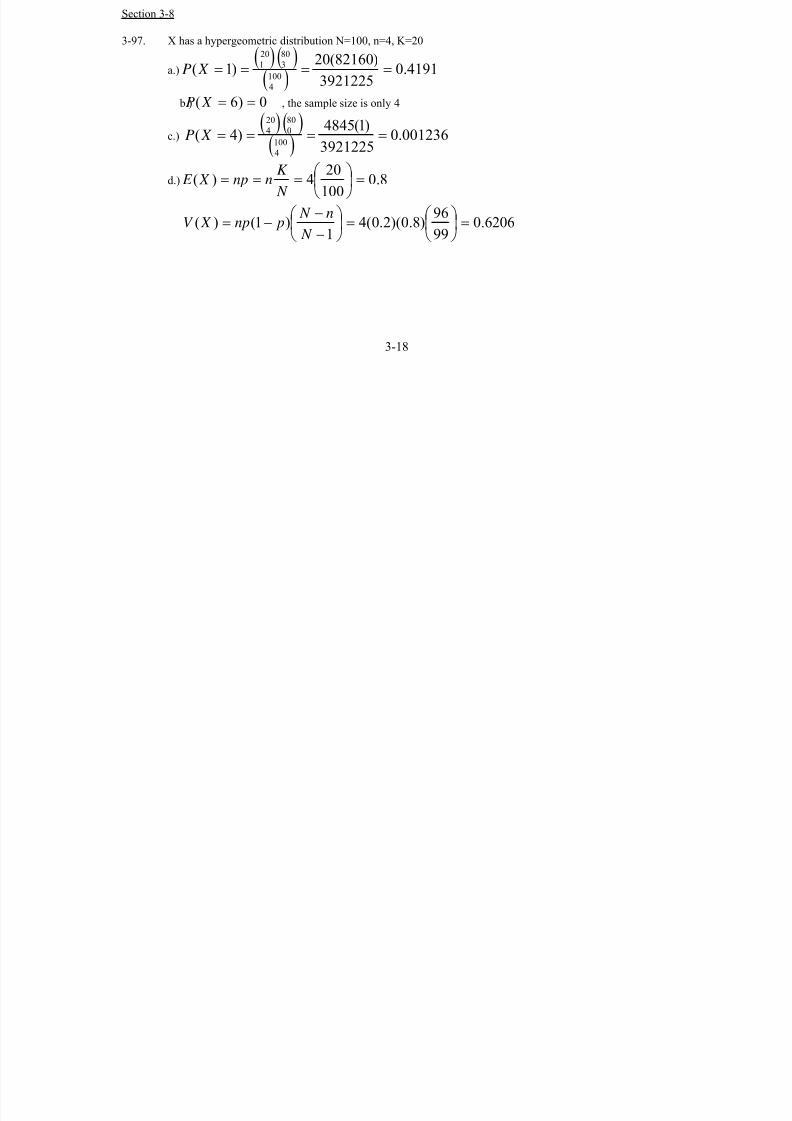
7/12/2019 Solution Manual Stats
http://slidepdf.com/reader/full/solution-manual-stats 60/588
Section 3-8
3-97. X has a hypergeometric distribution N=100, n=4, K=20
a.)( ) ( )( )
4191.03921225
)82160(20)1(
100
4
80
3
20
1 ==== X P
b.) , the sample size is only 40)6( == X P
c.)( ) ( )( )
001236.03921225
)1(4845)4(
100
4
80
0
20
4 ==== X P
d.) 8.0
100
204)( =⎟
⎠
⎞⎜
⎝
⎛ ===
N
K nnp X E
6206.099
96)8.0)(2.0(4
1)1()( =⎟
⎠
⎞⎜⎝
⎛ =⎟
⎠
⎞⎜⎝
⎛
−
−−=
N
n N pnp X V
3-18

7/12/2019 Solution Manual Stats
http://slidepdf.com/reader/full/solution-manual-stats 61/588
3-98. a)( ) ( )( )
4623.024/)17181920(
6/)1415164()1(
20
4
16
3
4
1 =×××
×××=== X P
b)( ) ( )( )
00021.024/)17181920(
1)4(
20
4
16
0
4
4 =×××
=== X P
c)
( )( )( )
( )( )( )
( )( )( )
9866.0
)2()1()0()2(
24
17181920
215166
61415164
2413141516
20
4
16
2
4
2
20
4
16
3
4
1
20
4
16
4
4
0
==
++=
=+=+==≤
⎟ ⎠
⎞⎜⎝
⎛ ×××
⎟ ⎠ ⎞⎜
⎝ ⎛ ××+×××+×××
X P X P X P X P
d) E(X) = 4(4/20) = 0.8
V(X) = 4(0.2)(0.8)(16/19) = 0.539
3-99. N=10, n=3 and K=4
0 1 2 3
0.0
0.1
0.2
0.3
0.4
0.5
x
P ( x )
3-100. (a) f(x) = /⎟⎟ ⎠
⎞⎜⎜⎝
⎛
−⎟⎟ ⎠
⎞⎜⎜⎝
⎛
x x 3
1224⎟⎟ ⎠
⎞⎜⎜⎝
⎛
3
36
(b) µ=E(X) = np= 3*24/36=2V(X)= np(1-p)(N-n)/(N-1) =2*(1-24/36)(36-3)/(36-1)=0.629
(c) P(X≤2) =1-P(X=3) =0.717
3-19

7/12/2019 Solution Manual Stats
http://slidepdf.com/reader/full/solution-manual-stats 62/588
3-101. Let X denote the number of men who carry the marker on the male chromosome for an increased risk for high
blood pressure. N=800, K=240 n=10
a) n=10
( )( )( )
( )( )1201.0)1(
!790!10!800
!551!9!560
!239!1!240
800
10
560
9
240
1 ==== X P
b) n=10
)]1()0([1)1(1)1( =+=−=≤−=> X P X P X P X P
( )( )( )
( )( )0276.0)0(
!790!10!800
!550!10!560
!240!0!240
800
10
560
10
240
0 ==== X P
8523.0]1201.00276.0[1)1(1)1( =+−=≤−=> X P X P
3-102. Let X denote the number of cards in the sample that are defective.
a)
( )( )( )
9644.00356.01)1(
0356.0)0(
)0(1)1(
!120!20!140
!100!20!120
140
20
120
20
20
0
=−=≥
=====−=≥
X P
X P
X P X P
b)
( )( )( )
5429.04571.01)1(
4571.0!140!115
!120!135)0(
)0(1)1(
!120!20!140
!115!20!135
140
20
135
20
5
0
=−=≥
=====
=−=≥
X P
X P
X P X P
3-103. N=300
(a) K=243, n=3, P(X=1)=0.087
(b) P(X≥1)=0.9934
(c) K=26+13=39
P(X=1)=0.297
(d) K=300-18=282
P(X≥1)=0.9998
3-104. Let X denote the count of the numbers in the state's sample that match those in the player's
sample. Then, X has a hypergeometric distribution with N = 40, n = 6, and K = 6.
a)( )( )( )
7
1
40
6
34
0
6
6 1061.2!34!6
!40)6( −
−
×=⎟ ⎠
⎞⎜⎝
⎛ === X P
b)( )( )( ) ( )
5
40
6
40
6
34
1
6
5 1031.5346
)5( −×=×
=== X P
c)( )( )( )
00219.0)4(40
6
34
2
6
4 === X P
d) Let Y denote the number of weeks needed to match all six numbers. Then, Y has a geometric distribution with p =
3-20

7/12/2019 Solution Manual Stats
http://slidepdf.com/reader/full/solution-manual-stats 63/588
380,838,3
1and E(Y) = 1/p = weeks. This is more than 738 centuries!380,838,3
3-105. Let X denote the number of blades in the sample that are dull.
a)
( ) ( )( )
7069.0)0(1)1(
2931.0!33!48
!43!38)0(
)0(1)1(
!43!5
!48
!33!5
!38
48
5
38
5
10
0
==−=≥
=====
=−=≥
X P X P
X P
X P X P
b) Let Y denote the number of days needed to replace the assembly.
P(Y = 3) = 0607.0)7069.0(2931.0 2 =
c) On the first day,( )
8005.0!41!48
!43!46)0(
!43!5!48
!41!5!46
48
5
46
5
2
0 ===== X P
On the second day,
( )( )( ) 4968.0!37!48
!43!42
)0(!43!5
!48
!37!5!42
485
42
5
6
0
===== X P
On the third day, P(X = 0) = 0.2931 from part a. Therefore,
P(Y = 3) = 0.8005(0.4968)(1-0.2931) = 0.2811.
3-106. a) For Exercise 3-97, the finite population correction is 96/99.
For Exercise 3-98, the finite population correction is 16/19.
Because the finite population correction for Exercise 3-97 is closer to one, the binomial approximation to
the distribution of X should be better in Exercise 3-97.
b) Assuming X has a binomial distribution with n = 4 and p = 0.2,
( )
( ) 0016.08.02.0)4(
4096.08.02.0)1(
044
4
314
1
===
===
X P
X P
The results from the binomial approximation are close to the probabilities obtained in Exercise
3-97.
c) Assume X has a binomial distribution with n = 4 and p = 0.2. Consequently, P(X = 1) and
P(X = 4) are the same as computed in part b. of this exercise. This binomial approximation is
not as close to the true answer as the results obtained in part b. of this exercise.
d) From Exercise 3-102, X is approximately binomial with n = 20 and p = 20/140 = 1/7.
( )( ) ( ) 9542.00458.01)0(1)1(20
760
7120
0 =−===−=≥ X P X P
finite population correction is 120/139=0.8633
From Exercise 3-92, X is approximately binomial with n = 20 and p = 5/140 =1/28
( )( ) ( ) 5168.04832.01)0(1)1(20
28270
28120
0 =−===−=≥ X P X P
finite population correction is 120/139=0.8633
3-21

7/12/2019 Solution Manual Stats
http://slidepdf.com/reader/full/solution-manual-stats 64/588
Section 3-9
3-107. a) P Xe
e( )!
.= = = =−
−04
000183
4 04
b) P X P X P X P X( ) ( ) ( ) (≤ = = + = )+ =2 0 1 2
= + +
=
−− −
e e e44 1 4 2
41
42
0 2381
! !
.
c) P Xe
( )!
.= = =−
44
401954
4 4
d) P Xe
( )!
.= = =−
84
80 0298
4 8
3-108 a) P X e( ) ..= = =−0 0 67030 4
b) P X ee e
( )( . )
!
( . )
!..
. .
≤ = + + =−− −
20 4
1
0 4
20 99210 4
0 4 0 4 2
c) P X
e
( )
( . )
! .
.
= = =
−
4
0 4
4 0 000715
0 4 4
d) P Xe
( )( . )
!.
.
= = = ×−
−80 4
8109 10
0 4 88
3-109. . Therefore, λ = −ln(0.05) = 2.996.P X e( ) .= = =−0 0λ 05
Consequently, E(X) = V(X) = 2.996.
3-110 a) Let X denote the number of calls in one hour. Then, X is a Poisson random variable with λ = 10.
P Xe
( )!
.= = =−
510
50 0378
10 5
.
b) P X ee e e
( )
! ! !
.≤ = + + + =−− − −
310
1
10
2
10
3
0 01031010 10 2 10 3
c) Let Y denote the number of calls in two hours. Then, Y is a Poisson random variable with
λ = 20. P Ye
( )!
.= = =−
1520
150 0516
20 15
d) Let W denote the number of calls in 30 minutes. Then W is a Poisson random variable with
λ = 5. P We
( )!
.= = =−
55
501755
5 5
3-111. λ =1, Poisson distribution. f(x) =e- λ λ x/x!
(a) P(X≥2)= 0.264
(b) In order that P(X≥1) = 1-P(X=0)=1-e- λ exceed 0.95, we need λ =3.
Therefore 3*16=48 cubic light years of space must be studied.
3-112. (a) λ =14.4, P(X=0)=6*10-7
(b) λ =14.4/5=2.88, P(X=0)=0.056
(c) λ =14.4*7*28.35/225=12.7
P(X≥1)=0.999997
(d) P(X≥28.8) =1-P(X ≤ 28) = 0.00046. Unusual.
3-113. (a) λ =0.61. P(X≥1)=0.4566
(b) λ =0.61*5=3.05, P(X=0)= 0.047.
3-22
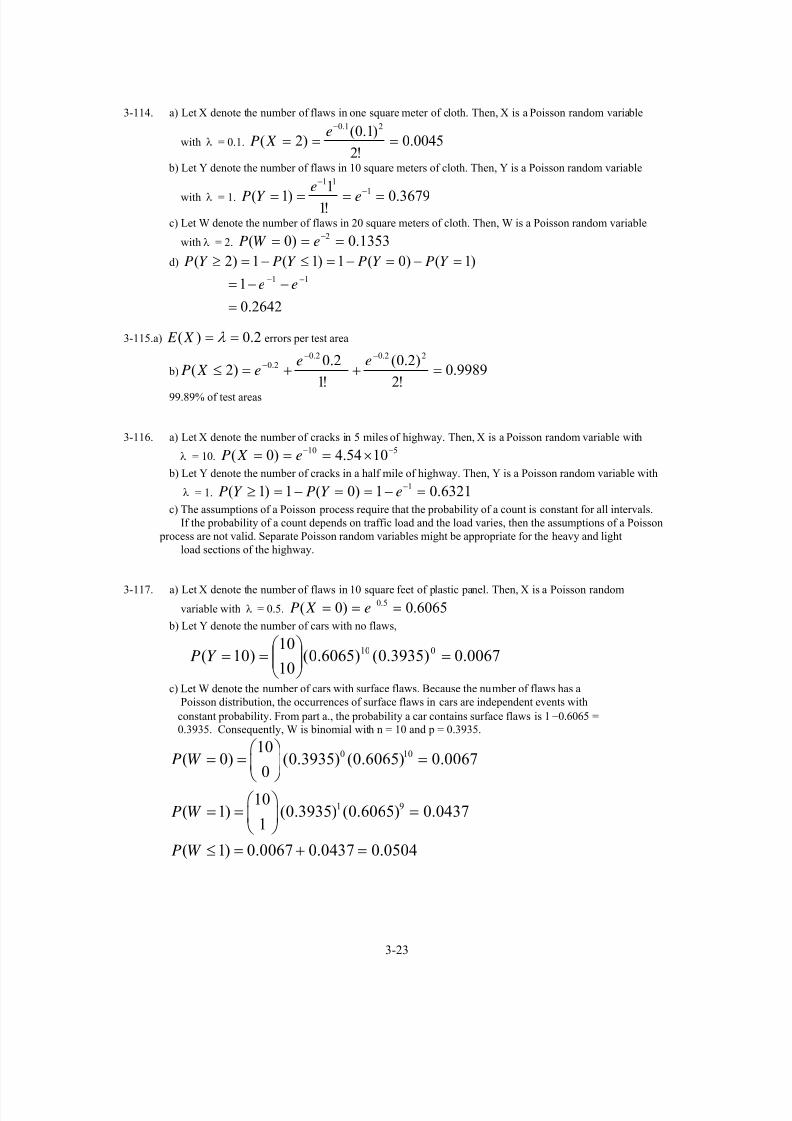
7/12/2019 Solution Manual Stats
http://slidepdf.com/reader/full/solution-manual-stats 65/588
3-114. a) Let X denote the number of flaws in one square meter of cloth. Then, X is a Poisson random variable
with = 0.1.λ 0045.0!2
)1.0()2(
21.0
===−
e X P
b) Let Y denote the number of flaws in 10 square meters of cloth. Then, Y is a Poisson random variable
with = 1.λ 3679.0!11)1( 1
11
==== −
−
eeY P
c) Let W denote the number of flaws in 20 square meters of cloth. Then, W is a Poisson random variable
with λ = 2. 1353.0)0( 2 === −eW P
d) )1()0(1)1(1)2( =−=−=≤−=≥ Y PY PY PY P
2642.0
1 11
=
−−= −−ee
3-115.a) 2.0)( == λ X E errors per test area
b) 9989.0
!2
)2.0(
!1
2.0)2(
22.02.02.0 =++=≤
−−− ee
e X P
99.89% of test areas
3-116. a) Let X denote the number of cracks in 5 miles of highway. Then, X is a Poisson random variable with
= 10.λ510 1054.4)0( −− ×=== e X P
b) Let Y denote the number of cracks in a half mile of highway. Then, Y is a Poisson random variable with
λ = 1. 6321.01)0(1)1( 1 =−==−=≥ −eY PY P
c) The assumptions of a Poisson process require that the probability of a count is constant for all intervals.
If the probability of a count depends on traffic load and the load varies, then the assumptions of a Poisson
process are not valid. Separate Poisson random variables might be appropriate for the heavy and light
load sections of the highway.
3-117. a) Let X denote the number of flaws in 10 square feet of plastic panel. Then, X is a Poisson random
variable with = 0.5.λ 6065.0)0( 5.0 === −e X P
b) Let Y denote the number of cars with no flaws,
0067.0)3935.0()6065.0(10
10)10( 010 =⎟⎟
⎠
⎞⎜⎜⎝
⎛ ==Y P
c) Let W denote the number of cars with surface flaws. Because the number of flaws has a
Poisson distribution, the occurrences of surface flaws in cars are independent events with
constant probability. From part a., the probability a car contains surface flaws is 1−0.6065 =
0.3935. Consequently, W is binomial with n = 10 and p = 0.3935.
0 10
1 9
10( 0) (0.3935) (0.6065) 0.0067
0
10( 1) (0.3935) (0.6065) 0.0437
1
( 1) 0.0067 0.0437 0.0504
P W
P W
P W
⎛ ⎞= = =⎜ ⎟
⎝ ⎠⎛ ⎞
= = =⎜ ⎟⎝ ⎠
≤ = + =
3-23

7/12/2019 Solution Manual Stats
http://slidepdf.com/reader/full/solution-manual-stats 66/588
3-118. a) Let X denote the failures in 8 hours. Then, X has a Poisson distribution with λ = 0.16.
8521.0)0( 16.0 === −e X P
b) Let Y denote the number of failure in 24 hours. Then, Y has a Poisson distribution with
λ = 0.48. 3812.01)0(1)1( 48 =−==−=≥ −eY PY P

7/12/2019 Solution Manual Stats
http://slidepdf.com/reader/full/solution-manual-stats 67/588
Supplemental Exercises
3-119.4
1
3
1
8
3
3
1
4
1
3
1
8
1)( =⎟
⎠
⎞⎜⎝
⎛ +⎟
⎠
⎞⎜⎝
⎛ +⎟
⎠
⎞⎜⎝
⎛ = X E ,
0104.04
1
3
1
8
3
3
1
4
1
3
1
8
1)(
2222
=⎟ ⎠
⎞⎜⎝
⎛ −⎟
⎠
⎞⎜⎝
⎛ ⎟ ⎠
⎞⎜⎝
⎛ +⎟
⎠
⎞⎜⎝
⎛ ⎟ ⎠
⎞⎜⎝
⎛ +⎟
⎠
⎞⎜⎝
⎛ ⎟ ⎠
⎞⎜⎝
⎛ = X V
3-120. a) 3681.0)999.0(001.01
1000)1( 9991 =⎟⎟
⎠
⎞⎜⎜⎝
⎛ == X P
( )
( ) ( )
999.0)999.0)(001.0(1000)(
1)001.0(1000)()d
9198.0
999.0001.02
1000999.0001.0
1
1000999.0001.0
0
1000)2()c
6319.0999.0001.00
10001)0(1)1() b
9982999110000
9990
==
==
=
⎟⎟ ⎠
⎞⎜⎜⎝
⎛ +⎟⎟
⎠
⎞⎜⎜⎝
⎛ +⎟⎟
⎠
⎞⎜⎜⎝
⎛ =≤
=⎟⎟ ⎠
⎞⎜⎜⎝
⎛ −==−=≥
X V
X E
X P
X P X P
3-121. a) n = 50, p = 5/50 = 0.1, since E(X) = 5 = np.
b) ( ) ( ) ( ) 112.09.01.02
509.01.01
509.01.00
50)2(
482
491
500
=⎟⎟ ⎠
⎞⎜⎜⎝
⎛ +⎟⎟ ⎠
⎞⎜⎜⎝
⎛ +⎟⎟ ⎠
⎞⎜⎜⎝
⎛ =≤ X P
c) ( ) ( ) 48050149 1051.49.01.050
509.01.0
49
50)49(
−×=⎟⎟ ⎠
⎞⎜⎜⎝
⎛ +⎟⎟
⎠
⎞⎜⎜⎝
⎛ =≥ X P
3-122. (a)Binomial distribution, p=0.01, n=12.
(b) P(X>1)=1-P(X≤1)= 1- - =0.0062120 )1(
0
12 p p −⎟⎟
⎠
⎞⎜⎜⎝
⎛ 141 )1(1
12 p p −⎟⎟
⎠
⎞⎜⎜⎝
⎛
(c) µ =E(X)= np =12*0.01 = 0.12
V(X)=np(1-p) = 0.1188 σ= )( X V = 0.3447
3-123. (a)12(0.5) 0.000244=
(b) = 0.22566 6
12 (0.5) (0.5)C 6
(c) 4189.0)5.0()5.0()5.0()5.0( 6612
6
7512
5 =+C C
3-124. (a) Binomial distribution, n=100, p=0.01.
(b) P(X≥1) = 0.634
(c) P(X≥2)= 0.264
3-24

7/12/2019 Solution Manual Stats
http://slidepdf.com/reader/full/solution-manual-stats 68/588
(d) µ=E(X)= np=100*0.01=1
V(X)=np(1-p) = 0.99
σ= )( X V =0.995
(e) Let pd= P(X≥2)= 0.264,
Y: # of messages requires two or more packets be resent.
Y is binomial distributed with n=10, pm=pd*(1/10)=0.0264
P(Y≥1) = 0.235
3-125 Let X denote the number of mornings needed to obtain a green light. Then X is a geometric random
variable with p = 0.20.
a) P(X = 4) = (1-0.2)30.2= 0.1024
b) By independence, (0.8)10
= 0.1074. (Also, P(X > 10) = 0.1074)
3-126 Let X denote the number of attempts needed to obtain a calibration that conforms to specifications. Then, X
is geometric with p = 0.6.
P(X ≤ 3) = P(X=1) + P(X=2) + P(X=3) = 0.6 + 0.4(0.6) + 0.42(0.6) = 0.936.
3-127. Let X denote the number of fills needed to detect three underweight packages. Then X is a negative
binomial random variable with p = 0.001 and r = 3.
a) E(X) = 3/0.001 = 3000
b) V(X) = [3(0.999)/0.0012] = 2997000. Therefore, σX = 1731.18
3-128. Geometric with p=0.1
(a) f(x)=(1-p)x-1 p=0.9(x-1)0.1
(b) P(X=5) = 0.94*0.1=0.0656
(c) µ=E(X)= 1/p=10
(d) P(X≤10)=0.651
3-129. (a) λ =6*0.5=3.P(X=0) = 0.0498
(b) P(X≥3)=0.5768
(c) P(X≤x) ≥0.9, x=5
(d) σ2= λ =6. Not appropriate.
3-130. Let X denote the number of totes in the sample that do not conform to purity requirements. Then, X has a
hypergeometric distribution with N = 15, n = 3, and K = 2.
3714.0!15!10
!12!131
3
15
3
13
0
2
1)0(1)1( =−=
⎟⎟ ⎠
⎞
⎜⎜⎝
⎛
⎟⎟ ⎠
⎞⎜⎜⎝
⎛ ⎟⎟ ⎠
⎞⎜⎜⎝
⎛
−==−=≥ X P X P
3-131. Let X denote the number of calls that are answered in 30 seconds or less. Then, X is a binomial random
variable with p = 0.75.
a) P(X = 9) = 1877.0)25.0()75.0(9
1019 =⎟⎟
⎠
⎞⎜⎜⎝
⎛
b) P(X ≥ 16) = P(X=16) +P(X=17) + P(X=18) + P(X=19) + P(X=20)
3-25

7/12/2019 Solution Manual Stats
http://slidepdf.com/reader/full/solution-manual-stats 69/588
4148.0)25.0()75.0(20
20)25.0()75.0(
19
20
)25.0()75.0(18
20)25.0()75.0(
17
20)25.0()75.0(
16
20
020119
218317416
=⎟⎟ ⎠
⎞⎜⎜⎝
⎛ +⎟⎟
⎠
⎞⎜⎜⎝
⎛ +
⎟⎟ ⎠
⎞⎜⎜⎝
⎛ +⎟⎟
⎠
⎞⎜⎜⎝
⎛ +⎟⎟
⎠
⎞⎜⎜⎝
⎛ =
c) E(X) = 20(0.75) = 15
3-132. Let Y denote the number of calls needed to obtain an answer in less than 30 seconds.
a) 0117.075.025.075.0)75.01()4( 33 ==−==Y P
b) E(Y) = 1/p = 1/0.75 = 4/3
3-133. Let W denote the number of calls needed to obtain two answers in less than 30 seconds. Then, W has a
negative binomial distribution with p = 0.75.
a) P(W=6) =5
10 25 0 75 0 01104 2⎛
⎝ ⎜
⎞
⎠⎟ =( . ) ( . ) .
b) E(W) = r/p = 2/0.75 = 8/3
3-134. a) Let X denote the number of messages sent in one hour. 1755.0
!5
5)5(
55
===−e
X P
b) Let Y denote the number of messages sent in 1.5 hours. Then, Y is a Poisson random variable with
λ =7.5. 0858.0!10
)5.7()10(
105.7
===−e
Y P
c) Let W denote the number of messages sent in one-half hour. Then, W is a Poisson random variable with
= 2.5.λ 2873.0)1()0()2( ==+==< W PW PW P
3-135X is a negative binomial with r=4 and p=0.0001
400000001.0/4/)( === pr X E requests
3-136. X ∼ Poisson(λ = 0.01), X ∼ Poisson(λ = 1)
9810.0!3)1(
!2)1(
!1)1()3(
3121111 =+++=≤−−−− eeeeY P
3-137. Let X denote the number of individuals that recover in one week. Assume the individuals are independent.
Then, X is a binomial random variable with n = 20 and p = 0.1. P(X ≥ 4) = 1 − P(X ≤ 3) = 1 − 0.8670 =
0.1330.
3-138. a.) P(X=1) = 0 , P(X=2) = 0.0025, P(X=3) = 0.01, P(X=4) = 0.03, P(X=5) = 0.065
P(X=6) = 0.13, P(X=7) = 0.18, P(X=8) = 0.2225, P(X=9) = 0.2, P(X=10) = 0.16
b.) P(X=1) = 0.0025, P(X=1.5) = 0.01, P(X=2) = 0.03, P(X=2.5) = 0.065, P(X=3) = 0.13
P(X=3.5) = 0.18, P(X=4) = 0.2225, P(X=4.5) = 0.2, P(X=5) = 0.16
3-139. Let X denote the number of assemblies needed to obtain 5 defectives. Then, X is a negative binomial
random variable with p = 0.01 and r=5.
a) E(X) = r/p = 500.
b) V(X) =(5* 0.99)/0.012 = 49500 and σX = 222.49
3-140. Here n assemblies are checked. Let X denote the number of defective assemblies. If P(X ≥ 1) ≥ 0.95, then
3-26

7/12/2019 Solution Manual Stats
http://slidepdf.com/reader/full/solution-manual-stats 70/588
P(X=0) ≤ 0.05. Now,
P(X=0) = and 0.99nn
n99)99.0()01.0(
0
0 =⎟⎟ ⎠
⎞⎜⎜⎝
⎛ n ≤ 0.05. Therefore,
07.298)95.0ln(
)05.0ln(
)05.0ln())99.0(ln(
=≥
≤
n
n
This would require n = 299.
3-141. Require f(1) + f(2) + f(3) + f(4) = 1. Therefore, c(1+2+3+4) = 1. Therefore, c = 0.1.
3-142. Let X denote the number of products that fail during the warranty period. Assume the units are
independent. Then, X is a binomial random variable with n = 500 and p = 0.02.
a) P(X = 0) = 4.1 x 10=⎟⎟ ⎠
⎞⎜⎜⎝
⎛ 5000 )98.0()02.0(0
500-5
b) E(X) = 500(0.02) = 10
c) P(X >2) = 1 − P(X ≤ 2) = 0.9995
3-143. 16.0)3.0)(3.0()7.0)(1.0()0( =+= X f
19.0)3.0)(4.0()7.0)(1.0()1( =+= X f
20.0)3.0)(2.0()7.0)(2.0()2( =+= X f
31.0)3.0)(1.0()7.0)(4.0()3( =+= X f
14.0)3.0)(0()7.0)(2.0()4( =+= X f
3-144. a) P(X ≤ 3) = 0.2 + 0.4 = 0.6
b) P(X > 2.5) = 0.4 + 0.3 + 0.1 = 0.8
c) P(2.7 < X < 5.1) = 0.4 + 0.3 = 0.7
d) E(X) = 2(0.2) + 3(0.4) + 5(0.3) + 8(0.1) = 3.9
e) V(X) = 22(0.2) + 32(0.4) + 52(0.3) + 82(0.1) − (3.9)2 = 3.09
3-145.
x 2 5.7 6.5 8.5
f(x) 0.2 0.3 0.3 0.2
3-146. Let X denote the number of bolts in the sample from supplier 1 and let Y denote the number of bolts in the
sample from supplier 2. Then, x is a hypergeometric random variable with N = 100, n = 4, and K = 30.
Also, Y is a hypergeometric random variable with N = 100, n = 4, and K = 70.
a) P(X=4 or Y=4) = P(X = 4) + P(Y = 4)
2408.0
4
1004
70
0
30
4
1000
70
4
30
=
⎟⎟ ⎠
⎞⎜⎜⎝
⎛
⎟⎟
⎠
⎞⎜⎜
⎝
⎛ ⎟⎟
⎠
⎞⎜⎜
⎝
⎛
+
⎟⎟ ⎠
⎞⎜⎜⎝
⎛
⎟⎟
⎠
⎞⎜⎜
⎝
⎛ ⎟⎟
⎠
⎞⎜⎜
⎝
⎛
=
3-27

7/12/2019 Solution Manual Stats
http://slidepdf.com/reader/full/solution-manual-stats 71/588
b) P[(X=3 and Y=1) or (Y=3 and X = 1)]= 4913.0
4
100
3
70
1
30
1
70
3
30
=
⎟⎟ ⎠
⎞⎜⎜⎝
⎛
⎟⎟ ⎠
⎞⎜⎜⎝
⎛ ⎟⎟ ⎠
⎞⎜⎜⎝
⎛ +⎟⎟
⎠
⎞⎜⎜⎝
⎛ ⎟⎟ ⎠
⎞⎜⎜⎝
⎛
=
3-147. Let X denote the number of errors in a sector. Then, X is a Poisson random variable with λ = 0.32768.
a) P(X>1) = 1 − P(X≤1) = 1 − e-0.32768
− e-0.32768
(0.32768) = 0.0433
b) Let Y denote the number of sectors until an error is found. Then, Y is a geometric random variable and
P = P(X ≥ 1) = 1 − P(X=0) = 1 − e-0.32768 = 0.2794
E(Y) = 1/p = 3.58
3-148. Let X denote the number of orders placed in a week in a city of 800,000 people. Then X is a Poisson
random variable with λ = 0.25(8) = 2.
a) P(X ≥ 3) = 1 − P(X ≤ 2) = 1 − [e-2 + e-2(2) + (e-222)/2!] = 1 − 0.6767 = 0.3233.
b) Let Y denote the number of orders in 2 weeks. Then, Y is a Poisson random variable with λ = 4, and
P(Y>2) =1- P(Y ≤ 2) = e-4
+ (e-4
41)/1!+ (e
-44
2)/2! =1 - [0.01832+0.07326+0.1465] = 0.7619.
3-149.a) hypergeometric random variable with N = 500, n = 5, and K = 125
2357.0115524.2
100164.6
5
500
5
375
0
125
)0( ==
⎟⎟ ⎠
⎞⎜⎜⎝
⎛
⎟⎟ ⎠
⎞⎜⎜⎝
⎛ ⎟⎟ ⎠
⎞⎜⎜⎝
⎛
= E
E f X
3971.0115525.2
)810855.8(125
5
500
4
375
1
125
)1( ==
⎟⎟
⎠
⎞⎜⎜
⎝
⎛
⎟⎟ ⎠
⎞⎜⎜⎝
⎛ ⎟⎟ ⎠
⎞⎜⎜⎝
⎛
= E
E f X
2647.0115524.2
)8718875(7750
5
500
3
375
2
125
)2( ==
⎟⎟ ⎠
⎞⎜⎜⎝
⎛
⎟⎟ ⎠
⎞⎜⎜⎝
⎛ ⎟⎟ ⎠
⎞⎜⎜⎝
⎛
= E
f X
0873.0115524.2
)70125(317750
5
500
2
375
3
125
)3( ==
⎟⎟ ⎠
⎞⎜⎜⎝
⎛
⎟⎟ ⎠
⎞⎜⎜⎝
⎛ ⎟⎟ ⎠
⎞⎜⎜⎝
⎛
= E
f X
01424.0115524.2
)375(9691375
5
500
1
375
4
125
)4( ==
⎟⎟ ⎠
⎞⎜⎜⎝
⎛
⎟⎟ ⎠
⎞⎜⎜⎝
⎛ ⎟⎟ ⎠
⎞⎜⎜⎝
⎛
= E
f X
3-28

7/12/2019 Solution Manual Stats
http://slidepdf.com/reader/full/solution-manual-stats 72/588
00092.0115524.2
83453.2
5
500
0
375
5
125
)5( ==
⎟⎟ ⎠
⎞⎜⎜⎝
⎛
⎟⎟ ⎠
⎞⎜⎜⎝
⎛ ⎟⎟ ⎠
⎞⎜⎜⎝
⎛
= E
E f X
b)
x 0 1 2 3 4 5 6 7 8 9 10
f(x) 0.0546 0.1866 0.2837 0.2528 0.1463 0.0574 0.0155 0.0028 0.0003 0.0000 0.0000
3-150. Let X denote the number of totes in the sample that exceed the moisture content. Then X is a binomial
random variable with n = 30. We are to determine p.
If P(X ≥ 1) = 0.9, then P(X = 0) = 0.1. Then , giving 30ln(1− p)=ln(0.1),
which results in p = 0.0739.
1.0)1()(0
30300 =−⎟⎟
⎠
⎞⎜⎜⎝
⎛ p p
3-151. Let t denote an interval of time in hours and let X denote the number of messages that arrive in time t.Then, X is a Poisson random variable with λ = 10t.
Then, P(X=0) = 0.9 and e-10t
= 0.9, resulting in t = 0.0105 hours = 37.8 seconds
3-152. a) Let X denote the number of flaws in 50 panels. Then, X is a Poisson random variable with
λ = 50(0.02) = 1. P(X = 0) = e-1
= 0.3679.
b) Let Y denote the number of flaws in one panel, then
P(Y ≥ 1) = 1 − P(Y=0) = 1 − e-0.02
= 0.0198. Let W denote the number of panels that need to be
inspected before a flaw is found. Then W is a geometric random variable with p = 0.0198 and
E(W) = 1/0.0198 = 50.51 panels.
c) 0198.01)0(1)1( 02.0 =−==−=≥ −eY PY P
Let V denote the number of panels with 1 or more flaws. Then V is a binomial random
variable with n=50 and p=0.0198
491500 )9802.0(0198.01
50)9802(.0198.00
50)2( ⎟⎟ ⎠ ⎞
⎜⎜⎝ ⎛ +⎟⎟
⎠ ⎞
⎜⎜⎝ ⎛ =≤V P
9234.0)9802.0(0198.02
50482 =⎟⎟
⎞⎜⎜⎛
+

7/12/2019 Solution Manual Stats
http://slidepdf.com/reader/full/solution-manual-stats 73/588
5-47
Mind-Expanding Exercises
5-94 By the independence,
)()...()(
)(...)()(
...)()...()(...),...,,(
2211
2211
21212211
2
2
1
1
21
21
p p
p p X
A
X
A
X
A
p p X X X
A A A
p p
A X P A X P A X P
dx x f dx x f dx x f
dxdxdx x f x f x f A X A X A X P
p
p
p
p
∈∈∈=
⎥⎥⎦
⎤
⎢⎢⎣
⎡
⎥⎥⎦
⎤
⎢⎢⎣
⎡
⎥⎥⎦
⎤
⎢⎢⎣
⎡=
=∈∈∈
∫∫∫
∫∫∫
5-95 ....)( 2211 p pcccY E μ μ μ +++=
Also,

7/12/2019 Solution Manual Stats
http://slidepdf.com/reader/full/solution-manual-stats 74/588
5-48
[ ]
[ ]p p X X X p p p
p X X X p p p p
dxdxdx x f x f x f xc xc
dxdx x f x f x f ccc xc xc xcY V
p
p
...)()...()()(...)(
...)()...()()...(...)(
2121
2
111
2121
2
22112211
21
21
μ μ
μ μ μ
−++−=
+++−+++=
∫∫
Now, the cross-term
[ ][ ] 0)()()()(
...)()...()())((
2222111121
212122112
1
21
21
=−−=
−−
∫∫∫
dx x f xdx x f xcc
dxdxdx x f x f x f x xcc
X X
p p X X X p
μ μ
μ μ
from the definition of the mean. Therefore, each cross-term in the last integral for V(Y)is zero and
).(...)(
)()(...)()()(
2
1
2
1
22
11
2
11
2
1 1
p p
p p X p p p X
X V c X V c
dx x f xcdx x f xcY V p
++=
−−= ∫∫ μ μ
5-96 cabcdydxdydx y x f
ba
XY
ba
== ∫∫∫∫0000
),( . Therefore, c = 1/ab. Then,
a
b
X cdy x f 1
0
)( == ∫ for 0 < x < a, and f y cdxY
a
b( ) = ∫ =
0
1 for 0 < y < b. Therefore,
(y)(x)f (x,y)=f f Y X XY for all x and y and X and Y are independent.
5-97 The marginal density of X is
.)()()()()()()(000
duuhk where xkgduuh xgduuh xg x f
bbb
X ∫∫∫ ==== Also,
.)()()(0
dvvglwhere ylh y f
a
Y
∫== Because (x,y) f XY is a probability density function,
.1)()()()(0000
=⎥⎦
⎤⎢⎣
⎡⎥⎦
⎤⎢⎣
⎡= ∫∫∫∫ duuhdvvgdydx yh xg
baba
Therefore, kl = 1 and
(y)(x)f (x,y)=f f Y X XY for all x and y.

7/12/2019 Solution Manual Stats
http://slidepdf.com/reader/full/solution-manual-stats 75/588
5-1
CHAPTER 5
Section 5-1
5-1. First, f(x,y) ≥ 0. Let R denote the range of (X,Y).
Then,
∑=++++=
R
y x f 1),(8
1
4
1
4
1
8
1
4
1
a) P(X < 2.5, Y < 3) = f(1.5,2)+f(1,1) = 1/8+1/4=3/8
b) P(X < 2.5) = f (1.5, 2) + f (1.5, 3) +f(1,1)= 1/8 + 1/4+1/4 = 5/8
c) P(Y < 3) = f (1.5, 2)+f(1,1) = 1/8+1/4=3/8
d) P(X > 1.8, Y > 4.7) = f ( 3, 5) = 1/8
e) E(X) = 1(1/4)+ 1.5(3/8) + 2.5(1/4) + 3(1/8) = 1.8125
E(Y) = 1(1/4)+2(1/8) + 3(1/4) + 4(1/4) + 5(1/8) = 2.875V(X)=E(X2)-[E(X)]2=[12(1/4)+1.52(3/8)+2.52(1/4)+32(1/8)]-1.81252=0.4961
V(Y)= E(Y2)-[E(Y)]2=[12(1/4)+22(1/8)+32(1/4)+42(1/4)+52(1/8)]-2.8752=1.8594
f) marginal distribution of X
x f(x)
1 ¼
1.5 3/8
2.5 ¼
3 1/8
g))5.1(
),5.1()(
5.1
X
XY
Y f
y f y f = and )5.1( X f = 3/8. Then,
y )(5.1y f
Y
2 (1/8)/(3/8)=1/3
3 (1/4)/(3/8)=2/3
h))2(
)2,()(
2
Y
XY
X f
x f x f = and )2(Y f = 1/8. Then,
x )(2y f
X
1.5 (1/8)/(1/8)=1
i) E (Y | X =1.5) = 2(1/3)+3(2/3) =2 1/3
j) Since f Y|1.5(y)≠f Y(y), X and Y are not independent
5-2 Let R denote the range of (X,Y). Because
1)654543432(),( =++++++++=∑ c y x f R
, 36c = 1, and c = 1/36
a) 4/1)432()3,1()2,1()1,1()4,1(36
1 =++=++=<= XY XY XY f f f Y X P
b) P(X = 1) is the same as part a. = 1/4
c) 3/1)543()2,3()2,2()2,1()2(36
1 =++=++== XY XY XY f f f Y P
d) 18/1)2()1,1()2,2(361 ===<< XY f Y X P

7/12/2019 Solution Manual Stats
http://slidepdf.com/reader/full/solution-manual-stats 76/588
5-2
e)
[ ] [ ]
[ ]
( ) ( ) ( ) 167.26/13321
)3,3()2,3()1,3(3
)3,2()2,2()1,2(2)3,1()2,1()1,1(1)(
36
15
36
12
36
9 ==×+×+×=
+++
+++++=
XY XY XY
XY XY XY XY XY XY
f f f
f f f f f f X E
639.0)3()2()1()( 36
152
6
13
36
122
6
13
36
92
6
13
=−+−+−= X V
639.0)(
167.2)(
=
=
Y V
Y E
f) marginal distribution of X
x )3,()2,()1,()( x f x f x f x f XY XY XY X ++=
1 1/4
2 1/3
3 5/12
g))1(
),1()( X
XY X Y
f y f y f =
y f yY X ( )
1 (2/36)/(1/4)=2/9
2 (3/36)/(1/4)=1/3
3 (4/36)/(1/4)=4/9
h))2(
)2,()(
Y
XY
Y X f
x f x f = and 3/1)2,3()2,2()2,1()2(
3612 ==++= XY XY XY Y f f f f
x f xX Y ( )
1 (3/36)/(1/3)=1/4
2 (4/36)/(1/3)=1/33 (5/36)/(1/3)=5/12
i) E (Y | X =1) = 1(2/9)+2(1/3)+3(4/9) = 20/9
j) Since f XY(x,y) ≠f X(x)f Y(y), X and Y are not independent.
5-3. ∑ =≥ R
y x f and y x f 1),(0),(
a)8
3
4
1
8
1)1,5.0()2,1()5.1,5.0( =+=−−+−−=<< XY XY f f Y X P
b)8
3)1,5.0()2,1()5.0( =−−+−−=< XY XY f f X P
c)8
7)1,5.0()1,5.0()2,1()5.1( =+−−+−−=< XY XY XY f f f Y P
d)8
5)2,1()1,5.0()5.4,25.0( =+=<> XY XY f f Y X P

7/12/2019 Solution Manual Stats
http://slidepdf.com/reader/full/solution-manual-stats 77/588
5-3
e)
41
81
21
41
81
81
81
21
41
81
)(2)(1)(1)(2)(
)(1)(5.0)(5.0)(1)(
=++−−=
=++−−=
Y E
X E
V(X)=(-1-1/8)2(1/8)+(-0.5-1/8)2(1/4)+(0.5-1/8)2(1/2)+(1-1/8)2(1/8)=0.4219
V(Y)=(-2-1/4)2(1/8)+(-1-1/4)2(1/4)+(1-1/4)2(1/2)+(2-1/4)2(1/8)=1.6875
f) marginal distribution of X
x )( x f X
-1 1/8
-0.5 ¼
0.5 ½
1 1/8
g))1(
),1()(
X
XY
X Y f
y f y f =
y f yY X ( )
2 1/8/(1/8)=1
h))1(
)1,()(
Y
XY
Y X f
x f x f =
x f xX Y ( )
0.5 ½/(1/2)=1
i) E ( X |Y =1) = 0.5
j) no, X and Y are not independent
5-4. Because X and Y denote the number of printers in each category,
40,0 =+≥≥ Y X and Y X
5-5. a) The range of (X,Y) is
3
2
10
y
x1 2 3
The problem needs probabilities to total one. Modify so that the probability of moderate
distortion is 0.04.
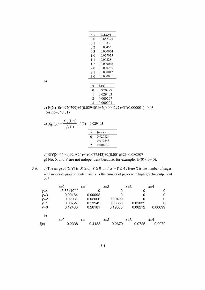
7/12/2019 Solution Manual Stats
http://slidepdf.com/reader/full/solution-manual-stats 78/588
5-4
x,y f xy(x,y)
0,0 0.857375
0,1 0.1083
0,2 0.00456
0,3 0.000064
1,0 0.027075
1,1 0.00228
1,2 0.000048
2,0 0.000285
2,1 0.000012
3,0 0.000001
b)
x f x(x)
0 0.970299
1 0.029403
2 0.0002973 0.000001
c) E(X)=0(0.970299)+1(0.029403)+2(0.000297)+3*(0.000001)=0.03
(or np=3*0.01)
d))1(
),1()(
1
X
XY
Y f
y f y f = , f x(1) = 0.029403
y f Y|1(x)
0 0.920824
1 0.077543
2 0.001632
e) E(Y|X=1)=0(.920824)+1(0.077543)+2(0.001632)=0.080807
g) No, X and Y are not independent because, for example, f Y(0)≠f Y|1(0).
5-6. a) The range of (X,Y) is 40,0 ≤+≥≥ Y X and Y X . Here X is the number of pages
with moderate graphic content and Y is the number of pages with high graphic output out
of 4.
x=0 x=1 x=2 x=3 x=4y=4 5.35x10-05 0 0 0 0y=3 0.00184 0.00092 0 0 0
y=2 0.02031 0.02066 0.00499 0 0y=1 0.08727 0.13542 0.06656 0.01035 0y=0 0.12436 0.26181 0.19635 0.06212 0.00699
b)
x=0 x=1 x=2 x=3 x=4f(x) 0.2338 0.4188 0.2679 0.0725 0.0070

7/12/2019 Solution Manual Stats
http://slidepdf.com/reader/full/solution-manual-stats 79/588
5-5
c)
E(X)=
2.1)0070.0(4)7248.0(3)2679.0(2)4188.0(1)2338.0(0)(4
0
==+++=∑ ii x f x
d) )3(
),3(
)(3 X
XY
Y f
y f
y f =
, f x(3) = 0.0725
Y f Y|3(y)
0 0.857
1 0.143
2 0
3 0
4 0
e) E(Y|X=3) = 0(0.857)+1(0.143) = 0.143
f) V(Y|X=3) = 02(0.857)+12(0.143)- 0.1432= 0.123
g) No, X and Y are not independent
5-7 a) The range of (X,Y) is 40,0 ≤+≥≥ Y X and Y X . X is the number of defective
items found with inspection device 1 and Y is the number of defective items found with
inspection device 2.
x=0 x=1 x=2 x=3 x=4y=0 1.94x10⁻¹⁹ 1.10x10⁻¹⁶ 2.35x10⁻¹⁴ 2.22x10⁻¹² 7.88x10⁻¹¹
y=1 2.59x10⁻¹⁶ 1.47x10⁻¹³ 3.12x10⁻¹¹ 2.95x10⁻⁹ 1.05x10⁻⁷
y=2 1.29x10⁻¹³ 7.31x10⁻¹¹ 1.56x10⁻⁸ 1.47x10⁻⁶ 5.22x10⁻⁵
y=3 2.86x10⁻¹¹ 1.62x10⁻⁸ 3.45x10⁻⁶ 3.26x10⁻⁴ 0.0116y=4 2.37x10⁻⁹ 1.35x10⁻⁶ 2.86x10⁻⁴ 0.0271 0.961
For x = 1,2,3,4 and y = 1,2,3,4
b)
x=0 x=1 x=2 x=3 x=4
f(x) 2.40 x 10⁻⁹ 1.36 x 10⁻⁶ 2.899 x 10⁻⁴ 0.0274 0.972
c) Because X has binomial distribution E ( X )= n( p) = 4*(0.993)=3.972
d) )()2(
),2()(2| y f
f
y f y f
X
XY
Y == , f x(2) = 2.899 x 10⁻⁴
y f Y|1(y)=f(y
⎥⎦
⎤⎢⎣
⎡⎟⎟ ⎠ ⎞
⎜⎜⎝ ⎛ ⎥
⎦
⎤⎢⎣
⎡⎟⎟ ⎠ ⎞
⎜⎜⎝ ⎛ = −− y y x x
y x y x f 44 )003.0()997.0(
4)007.0()993.0(
4),(
1,2,3,4for )007.0()993.0(4
),( 4 =⎥⎦
⎤⎢⎣
⎡⎟⎟ ⎠
⎞⎜⎜⎝
⎛ = − x
x y x f x x

7/12/2019 Solution Manual Stats
http://slidepdf.com/reader/full/solution-manual-stats 80/588
5-6
)
0 8.1 x 10⁻¹¹
1 1.08 x 10⁻⁷
2 5.37 x 10⁻⁵
3 0.0119
4 0.988
e) E(Y|X=2) = E(Y)= n( p)= 4(0.997)=3.988
f) V(Y|X=2) = V(Y)=n( p)(1- p)=4(0.997)(0.003)=0.0120
g) Yes, X and Y are independent.
5-8. a) 5.0)2,2,2()1,2,2()2,1,2()1,1,2()2( =+++== XYZ XYZ XYZ XYZ f f f f X P
b) 35.0)2,2,1()1,2,1()2,1( =+=== XYZ XYZ f f Y X P
c) c) 5.0)1,2,2()1,1,2()1,2,1()1,1,1()5.1( =+++=< XYZ XYZ XYZ XYZ f f f f Z P
d)
7.03.05.05.0)2,1()2()1()21(=−+===−=+====
Z X P Z P X P Z or X P
e) E(X) = 1(0.5) + 2(0.5) = 1.5
f) 3.005.01.02.015.0
10.005.0
)1(
)1,1()1|1( =
+++
+=
=
=====
Y P
Y X PY X P
g) 2.005.015.02.01.0
1.0
)2(
)2,1,1()2|1,1( =
+++=
=
========
Z P
Z Y X P Z Y X P
h) 4.015.010.0
10.0
)2,1(
)2,1,1()2,1|1( =
+=
==
=======
Z Y P
Z Y X P Z Y X P
i))2,1(
)2,1,()(
YZ
XYZ
YZ X f
x f x f = and 25.0)2,1,2()2,1,1()2,1( =+= XYZ XYZ YZ f f f
x )( x f YZ X
1 0.10/0.25=0.4
2 0.15/0.25=0.6
5-9. (a) f XY(x,y)= (10%)x(30%)y (60%)4-x-y , for X+Y<=4

7/12/2019 Solution Manual Stats
http://slidepdf.com/reader/full/solution-manual-stats 81/588
5-7
f XY(x,y) x y
0.1296 0 0
0.0648 0 1
0.0324 0 2
0.0162 0 30.0081 0 4
0.0216 1 0
0.0108 1 1
0.0054 1 2
0.0027 1 3
0.0036 2 0
0.0018 2 1
0.0009 2 2
0.0006 3 0
0.0003 3 1
0.0001 4 0
(b) f X(x)= P(X=x) = ∑≤+ 4
),(Y X
XY y x f .
f X(x) x
0.2511 0
0.0405 1
0.0063 2
0.0009 3
0.0001 4
(c) E(X)=∑ )( x xf X =0*0.2511+1*0.0405+2*0.0063+3*0.0009+4*0.0001= 0.0562
(d) f(y|X=3) = P(Y=y, X=3)/P(X=3)
P(Y=0, X=3) = C24
1 C43/ C
404 P(Y=1, X=3) = C12
1 C43/ C
404
P(X=3) = C361 C4
3/ C40
4, from the hypergeometric distribution with N=40, n=4, k=4, x=3
Therefore
f(0|X=3) = [C241 C4
3/ C40
4]/[ C36
1 C43/ C
404] = C24
1/ C36
1 = 2/3
f(1|X=3) = [C121 C4
3/ C40
4]/[ C36
1 C43/ C
404] = C12
1/ C36
1 = 1/3
f Y|3(y) y x
2/3 0 3
1/3 1 3
0 2 3
0 3 30 4 3
(e) E(Y|X=3)=0(0.6667)+1(0.3333)=0.3333
(f) V(Y|X=3)=(0-0.3333)2(0.6667)+(1-0.3333)2(0.3333)=0.0741
(g) f X(0)= 0.2511, f Y(0)=0.1555, f X(0) * f Y(0)= 0.039046 ≠ f XY(0,0) = 0.1296
X and Y are not independent.
5-10. (a) P(X<5) = 0.44+0.04=0.48

7/12/2019 Solution Manual Stats
http://slidepdf.com/reader/full/solution-manual-stats 82/588
5-8
(b) E(X)= 0.43*23+0.44*4.2+0.04*11.4+0.05*130+0.04*0=18.694
(c) PX|Y=0(X) = P(X=x,Y=0)/P(Y=0) = 0.04/0.08 = 0.5 for x=0 and 11.4
(d) P(X<6|Y=0) = P(X=0|Y=0) = 0.5
(e) E(X|Y=0)=11.4*0.5+0*0.5 = 5.7
5-11 a) percentage of slabs classified as high = p1 = 0.05
percentage of slabs classified as medium = p2 = 0.85 percentage of slabs classified as low = p3 = 0.10
b) X is the number of voids independently classified as high X ≥ 0
Y is the number of voids independently classified as medium Y ≥ 0
Z is the number of with a low number of voids and Z ≥ 0 and X +Y + Z = 20
c) p1 is the percentage of slabs classified as high.
d) E(X)=np1 = 20(0.05) = 1
V(X)=np1 (1- p1)= 20(0.05)(0.95) = 0.95
e) 0)3,17,1( ==== Z Y X P Because the point 20)3,17,1( ≠ is not in the range of (X,Y,Z).
f)
07195.0010.085.005.0!3!17!0
!20
)3,17,1()3,17,0()3,17,1(
3170 =+=
===+======≤ Z Y X P Z Y X P Z Y X P
Because the point 20)3,17,1( ≠ is not in the range of (X,Y,Z).
g) Because X is binomial, ( ) ( ) 7358.095.005.095.005.0)1( 19120
1
20020
0 =+=≤ X P
h) Because X is binomial E(Y) = np = 20(0.85) = 17
i) The probability is 0 because x+y+z>20
j))17(
)17,2()17|2(
=
=====
Y P
Y X PY X P . Now, because x+y+z = 20,
P(X=2, Y=17) = P(X=2, Y=17, Z=1) = 0540.010.085.005.0!1!17!2
!20 1172 =
2224.02428.0
0540.0
)17(
)17,2()17|2( ==
=
=====
Y P
Y X PY X P
k)
⎟⎟ ⎠
⎞⎜⎜⎝
⎛
=
==+⎟⎟
⎠
⎞⎜⎜⎝
⎛
=
==+
⎟⎟
⎠
⎞⎜⎜
⎝
⎛
=
==+⎟⎟
⎠
⎞⎜⎜
⎝
⎛
=
====
)17(
)17,3(3
)17(
)17,2(2
)17(
)17,1(1
)17(
)17,0(0)17|(
Y P
Y X P
Y P
Y X P
Y P
Y X P
Y P
Y X PY X E
1
2428.0
008994.03
2428.0
05396.02
2428.0
1079.01
2428.0
07195.00)17|(
=
⎟ ⎠
⎞⎜⎝
⎛ +⎟
⎠
⎞⎜⎝
⎛ +⎟
⎠
⎞⎜⎝
⎛ +⎟
⎠
⎞⎜⎝
⎛ ==Y X E

7/12/2019 Solution Manual Stats
http://slidepdf.com/reader/full/solution-manual-stats 83/588
5-9
5-12. a) The range consists of nonnegative integers with x+ y+ z = 4.
b) Because the samples are selected without replacement, the trials are not independent
and the joint distribution is not multinomial.
c))2(
)2,()2|(Y
XY
f x f Y x X P ===
( )( )( )( )
( )( )( )( )
( )( )( )( )
( )( )( )( )
( )( )( )( )
( )( )( )( )0440.0)2and2(
1758.0)2and1(
1098.0)2and0(
3296.00440.01758.01098.0)2(
15
4
6
1
5
2
4
1
15
4
6
1
5
2
4
1
15
4
6
2
5
2
4
0
15
4
6
0
5
2
4
2
15
4
6
1
5
2
4
1
15
4
6
2
5
2
4
0
====
====
====
=++=++==
Y X P
Y X P
Y X P
Y P
x )2,( x f XY
0 0.1098/0.3296=0.3331
1 0.1758/0.3296=0.5334
2 0.0440/0.3296=0.1335
d)
P(X=x, Y=y, Z=z) is the number of subsets of size 4 that contain x printers with graphics
enhancements, y printers with extra memory, and z printers with both features divided by
the number of subsets of size 4.
( )( )( )( )15
4
654
),,(z y x
z Z yY x X P ==== for x+y+z = 4.
( )( )( )( )
1758.0)1,2,1(15
4
6
1
5
2
4
1 ===== Z Y X P
e)( )( )( )
( )2198.0)2,1,1()1,1(
15
4
6
2
5
1
4
1 ======== Z Y X PY X P
f) The marginal distribution of X is hypergeometric with N = 15, n = 4, K = 4. Therefore,
E(X) = nK/N = 16/15 and V(X) = 4(4/15)(11/15)[11/14] = 0.6146.g)
( )( )( )( )[ ] ( )( )
( )[ ] 4762.0
)1(/)1,2,1()1|2,1(
154
93
61
154
61
52
41 ==
======== Z P Z Y X P Z Y X P
h)
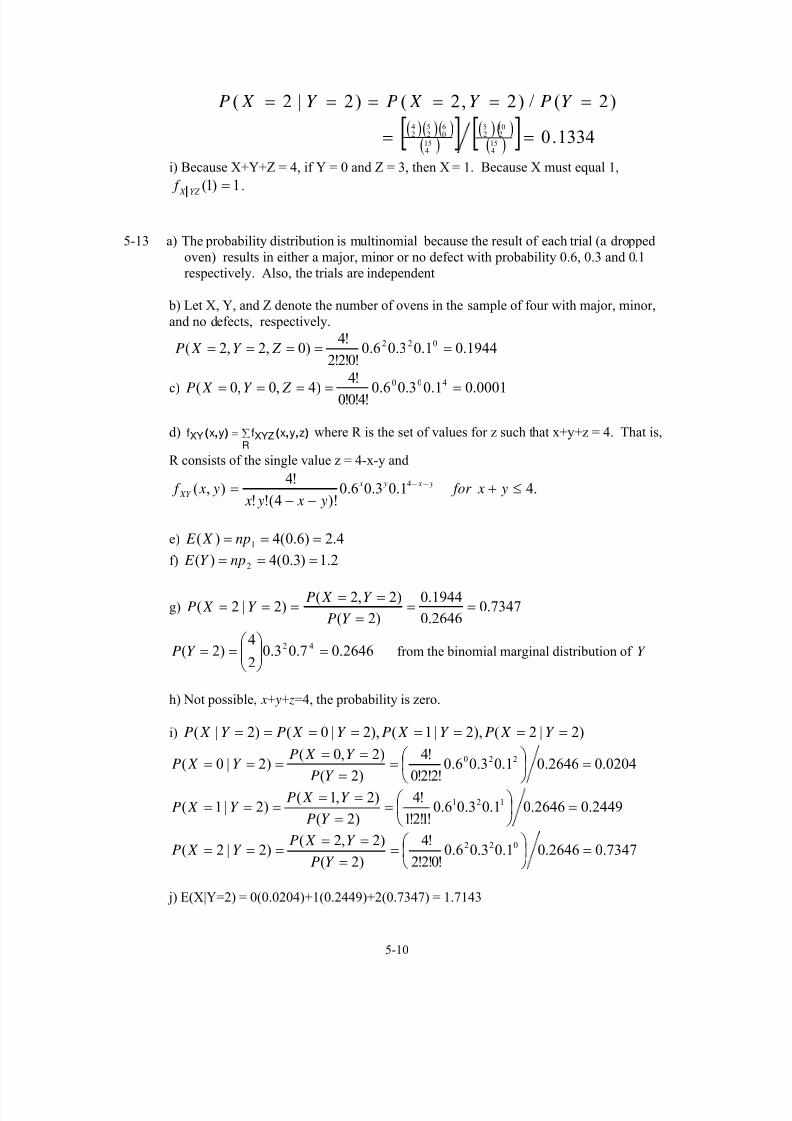
7/12/2019 Solution Manual Stats
http://slidepdf.com/reader/full/solution-manual-stats 84/588
5-10
( )( )( )( )[ ] ( ) ( )
( )[ ] 1334.0
)2(/)2,2()2|2(
154
102
52
154
60
52
42 ==
====== Y PY X PY X P
i) Because X+Y+Z = 4, if Y = 0 and Z = 3, then X = 1. Because X must equal 1,
1)1(=
YZ X f .
5-13 a) The probability distribution is multinomial because the result of each trial (a dropped
oven) results in either a major, minor or no defect with probability 0.6, 0.3 and 0.1
respectively. Also, the trials are independent
b) Let X, Y, and Z denote the number of ovens in the sample of four with major, minor,
and no defects, respectively.
1944.01.03.06.0!0!2!2
!4)0,2,2( 022 ===== Z Y X P
c) 0001.01.03.06.0!4!0!0
!4)4,0,0( 400 ===== Z Y X P
d) f x y f x y zXY XYZR
( , ) ( , , )= ∑ where R is the set of values for z such that x+y+z = 4. That is,
R consists of the single value z = 4-x-y and
.41.03.06.0)!4(!!
!4),( 4 ≤+
−−= −−
y x for y x y x
y x f y x y x
XY
e) 4.2)6.0(4)( 1 === np X E
f) 2.1)3.0(4)( 2 === npY E
g) === )2|2( Y X P 7347.02646.0
1944.0
)2(
)2,2(==
=
==
Y P
Y X P
2646.07.03.02
4)2( 42 =⎟⎟
⎠
⎞⎜⎜⎝
⎛ ==Y P from the binomial marginal distribution of Y
h) Not possible, x+ y+ z=4, the probability is zero.
i) )2|2(),2|1(),2|0()2|( ======== Y X PY X PY X PY X P
0204.02646.01.03.06.0!2!2!0
!4
)2(
)2,0()2|0( 220 =⎟
⎠
⎞⎜⎝
⎛ =
=
=====
Y P
Y X PY X P
2449.02646.01.03.06.0!1!2!1
!4
)2(
)2,1()2|1( 121 =⎟
⎠
⎞⎜⎝
⎛ =
=
=====
Y P
Y X PY X P
7347.02646.01.03.06.0!0!2!2
!4
)2(
)2,2()2|2( 022 =⎟
⎠
⎞⎜⎝
⎛ =
=
=====
Y P
Y X PY X P
j) E(X|Y=2) = 0(0.0204)+1(0.2449)+2(0.7347) = 1.7143

7/12/2019 Solution Manual Stats
http://slidepdf.com/reader/full/solution-manual-stats 85/588
5-11
5-14 Let X, Y, and Z denote the number of bits with high, moderate, and low distortion. Then,
the joint distribution of X, Y, and Z is multinomial with n =3 and
95.0,04.0,01.0 321 === pand p p .
a)
5012 102.195.004.001.0!0!1!2
!3)0,1,2()1,2(
−×======== Z Y X PY X P
b) 8574.095.004.001.0!3!0!0
!3)3,0,0( 300 ===== Z Y X P
c) X has a binomial distribution with n = 3 and p = 0.01. Then, E(X) = 3(0.01) = 0.03
and V(X) = 3(0.01)(0.99) = 0.0297.
d) First find )2|( =Y X P
0046.095.0)04.0(01.0!1!2!0
!395.0)04.0(01.0
!0!2!1
!3
)1,2,0()0,2,1()2(
12002 =+=
===+===== Z Y X P Z Y X PY P
98958.0004608.095.004.001.0!1!2!0
!3
)2(
)2,0()2|0( 120 =⎟
⎠
⎞⎜⎝
⎛ =
=
=====
Y P
Y X PY X P
01042.0004608.095.004.001.0!1!2!1
!3
)2(
)2,1()2|1( 021 =⎟
⎠
⎞⎜⎝
⎛ =
=
=====
Y P
Y X PY X P
)2|( =Y X E 01042.0)01042.0(1)98958.0(0 =+=
01031.0)01042.0(01042.0))(()()2|( 222 =−=−== X E X E Y X V
5-15. (a) f XYZ(x,y,z)
f XYZ(x,y,z)
Selects(X) Updates(Y)
Inserts(Z)
0.43 23 11 12
0.44 4.2 3 1
0.04 11.4 0 0
0.05 130 120 0
0.04 0 0 0
(b)PXY|Z=0
PXY|Z=0(x,y)
Selects(X) updates(Y)
Inserts(Z)
4/13 = 0.3077 11.4 0 0
5/13 = 0.3846 130 120 0
4/13= 0.3077 0 0 0
(c) P(X<6, Y<6|Z=0)=P(X=Y=0)=0.3077

7/12/2019 Solution Manual Stats
http://slidepdf.com/reader/full/solution-manual-stats 86/588
5-12
(d) E(X|Y=0,Z=0) =0.5*11.4+0.5*0=5.7
5-16 a) Let X, Y, and Z denote the risk of new competitors as no risk, moderate risk,
and very high risk. Then, the joint distribution of X, Y, and Z is multinomial with n =12
and 15.0,72.0,13.0 321 === pand p p . X, Y and Z ≥ 0 and x+y+z=12
b) )1,3,1( === Z Y X P = 0, not possible since x+y+z≠12
c)
7358.02924.03012.01422.0
85.015.02
1285.015.0
1
1285.015.0
0
12)2( 102111120
=++=
⎟⎟ ⎠
⎞⎜⎜⎝
⎛ +⎟⎟
⎠
⎞⎜⎜⎝
⎛ +⎟⎟
⎠
⎞⎜⎜⎝
⎛ =≤ Z P
d) 0)10,1|2( ==== X Y Z P
e)
8988
201011100210
1089.61004.21097.11072.4
15.072.013.0!2!0!10
!1215.072.013.0
!1!1!10
!1215.072.013.0
!0!2!10
!12
)2,0,10()1,1,10()0,2,10()10(
−−−− =++=
++=
===+===+=====
x x x x
Z Y X P Z Y X P Z Y X P X P
9698.0
1089.615.072.013.010!1!1!
12!1089.615.072.013.0
10!2!0!
12!
)10(
)10,1,1(
)10(
)10,2,0()10|1(
111080210
=
+=
=
===+
=
=====≤
−− x x
X P
X Y Z P
X P
X Y Z P X Z P
f)
2852.0
1089.615.072.013.010!1!1!
12!
)10(
)10,1,1()10|1,1(
81110
=
=
=
=====≤≤
− x
X P
X Y Z P X Z Y P
g)
345.0
1089.6/))1004.2(2)1097.1(1)1072.4(0()10|( 8988
=
++== −−−− x x x x X Z E

7/12/2019 Solution Manual Stats
http://slidepdf.com/reader/full/solution-manual-stats 87/588
5-13
Section 5-2
5-17 Determine c such that .)5.4(4
813
02
3
0
3
0
3
02
3
0
22
ccdy yc xydxdycy x ===∫ ∫∫
Therefore, c = 4/81.
a) 4444.0))(2()2()3,2(2
9
81
4
3
0
3
0
81
4
2
0
81
4 ====<< ∫ ∫∫ ydy xydxdyY X P
b) P(X < 2.5) = P(X < 2.5, Y < 3) because the range of Y is from 0 to 3.
6944.0)125.3()125.3()3,5.2(29
814
3
0
3
0
814
5.2
0
814 ====<< ∫ ∫∫ ydy xydxdyY X P
c) 5833.0)5.4()5.21(5.2
1281
18
5.2
1
5.2
1
814
3
0
814
2
====<< ∫ ∫∫y
ydy xydxdyY P
d)
3733.0)88.2()88.2()5.21,8.1(
5.2
1
5.2
1
2
)15.2(
814814
3
8.1
814
2
∫ ∫∫ ====<<>−
ydy xydxdyY X P
e) 29)(3
029
4
3
0
3
0
81
4
3
0
2
81
42
==== ∫ ∫∫y
ydy ydxdy x X E
f) ∫∫ ∫ ===<<4
0
4
0
0
0
814 00)4,0( ydy xydxdyY X P
g) 30)5.4(),()(9
2
81
4
3
0
81
4
3
0
<<==== ∫∫ x for x ydy xdy y x f x f x XY X
.
h) y
y
f
y f
y f X
XY
Y 9
2
9
2
81
4
5.1)5.1(
)5.1(
)5.1(
),5.1(
)( === for 0 < y < 3.
i) E(Y|X=1.5) = 227
2
9
2
9
23
0
3
0
32
3
0
===⎟ ⎠
⎞⎜⎝
⎛ ∫∫
ydy ydy y y
j)9
40
9
4
9
1
9
2)()5.1|2(
2
0
2
2
0
5.1| =−=====< ∫ y ydy y f X Y P Y
k) x x
f
x f x f
Y
XY
X 9
2
9
2
81
4
2)2(
)2(
)2(
)2,()( === for 0 < x < 3.

7/12/2019 Solution Manual Stats
http://slidepdf.com/reader/full/solution-manual-stats 88/588
5-14
5-18.
[ ]
( ) [ ] c x xdx xc
dx x x x
dx xydydx y xc
x x
x
x
y
x
x
242224
)2(
)(
3
0
2
3
0
3
0
2
2
2
)2(
3
0
3
0
2
2
2
22
2
=+=+=
−−++=
+=+
∫
∫
∫ ∫∫
+
++
Therefore, c = 1/24.
a) P(X < 1, Y < 2) equals the integral of ),( y x f XY over the following region.
0
0 1 2
2
x
y
Then,
10417.02241
2224
1
24
1)(
24
1)2,1(
1
02
2
3
0
2
3
1
0
1
0
2
2
2
3
22
=⎥⎦⎤⎢
⎣⎡ −+
=−+=+=+=<< ∫∫ ∫∫
x
x
x
y
x
x x
dx xdx xydydx y xY X P
b) P(1 < X < 2) equals the integral of ),( y x f XY over the following region.
00 1 2
2
x
y
∫
∫ ∫∫
=⎥⎦
⎤⎢⎣
⎡+=+=
+=+=<<++
3
0
6
12
1
2
2
1
2
1
2
2
2
.2224
1)24(
24
1
24
1)(
24
1)21(
2
x xdx x
dx xydydx y x X P x
x
y x
x

7/12/2019 Solution Manual Stats
http://slidepdf.com/reader/full/solution-manual-stats 89/588
5-15
c) P(Y > 1) is the integral of f x yXY ( , ) over the following region.
9792.002083.01
2
1
2
1
224
11
2
3
2
1
24
11
)2
(24
11)(1)1(1)1(
1
0
321
0
2
1
0
1
0
121
241
=−=
⎟⎟ ⎠
⎞⎜⎜⎝
⎛ −+−=−+−=
+−=+−=≤−=>
∫
∫ ∫∫
x x
dx x x
y xydydx y xY PY P
x x
d) P(X < 2, Y < 2) is the integral of f x yXY( , ) over the following region.
0
02
2
x
y
∫
∫ ∫∫
=⎥⎦
⎤⎢⎣
⎡+=+=
+=+=++
3
0
3
0
23
2
3
0
3
0
2
2
2
2
8
15
3
4
24
1)24(
24
1
24
1)(
24
1)(
2
x x
dx x x
dx y xdydx y x x X E x
x
xy
x
x
e)
∫
∫ ∫∫
=⎥⎦
⎤⎢⎣
⎡+=+=
+=+=++
3
0
3
0
23
2
3
0
3
0
2
2
2
2
8
15
3
4
24
1)24(
24
1
24
1)(
24
1)(
2
x x
dx x x
dx y xdydx y x x X E x
x
xy
x
x

7/12/2019 Solution Manual Stats
http://slidepdf.com/reader/full/solution-manual-stats 90/588
5-16
f)
320
31707
8
15
202
3
4
4
3
24
1
8
15)
4
443(
24
1
8
15
24
1
8
15)(
24
1)(
23
0
52
34
23
0
423
23
0
3
0
2
2
3
2 2
222
=⎟ ⎠
⎞⎜⎝
⎛ −⎥
⎦
⎤⎢⎣
⎡−++=
⎟
⎠
⎞⎜
⎝
⎛ −−++=
⎟ ⎠
⎞⎜⎝
⎛ −+=⎟
⎠
⎞⎜⎝
⎛ −+=
∫
∫ ∫∫++
x x
x x
dx x
x x x
dx y xdydx y x x X V x
x
y x
x
x
g) )( x f X is the integral of ),( y x f XY over the interval from x to x+2. That is,
12
1
624
1)(
24
1)(
2
2
22
+=⎥⎦
⎤⎢⎣
⎡+=+=
++
∫x
xydy y x x f x
x
y
x
x
X for 0 < x < 3.
h)
6
1)(
12
1
6
1
)1(24
1
)1(
),1(
1
y y f
y
f
y f
Y X
XY +
===+
+
for 1 < y < 3.
See the following graph,
0
0 1 2
2
x
y
1
f (y) defined over this line segmentY|1
i) E(Y|X=1) = 111.2326
1)(
6
1
6
13
1
3
1
323
1
2
∫ ∫ =⎟⎟ ⎠
⎞⎜⎜⎝
⎛ +=+=⎟
⎠
⎞⎜⎝
⎛ + y ydy y ydy
y y
j) ==> )1|2( X Y P 5833.026
1)1(
6
1
6
13
2
3
2
23
2
∫ ∫ =⎟⎟ ⎠
⎞⎜⎜⎝
⎛ +=+=⎟
⎠
⎞⎜⎝
⎛ + y ydy ydy
y
k) )2(
)2,(
2)(
Y
XY
f
x f
X x f = . Here )( y f Y is determined by integrating over x. There are
three regions of integration. For 20 ≤< y the integration is from 0 to y. For 32 ≤< y
the integration is from y-2 to y. For 53 << y the integration is from y to 3. Because
the condition is y=2, only the first integration is needed.
160
2
0
22
24
1)(
24
1)(
y y
x
y
Y xydx y x y f =⎥⎦
⎤⎢⎣
⎡+=+= ∫ for 20 ≤< y .

7/12/2019 Solution Manual Stats
http://slidepdf.com/reader/full/solution-manual-stats 91/588
5-17
0
0 1 2
2
x
y
1
f (x) defined over this line segmentX|2
Therefore, 4/1)2( =Y f and6
2
4/1
)2(24
1
)(2
+=
+=
x x
x f X
for 0 < x < 3
5-19 .8
81
822
3
0
3
0
43
0
3
0
2
0
c x
dx x
cdx y
xc x xydyd c
x x
∫ ∫ ∫∫ === Therefore, c = 8/81
a) P(X<1,Y<2)= .81
1
8
1
81
8
281
8
81
81
0
1
0
3
0 =⎟ ⎠
⎞
⎜⎝
⎛
==∫ ∫∫ dx
x
x xydyd
x
b) P(1<X<2) = .27
5
8
)12(
81
8
881
8
281
8
81
8 42
1
2
1
422
1 0
=−
⎟ ⎠
⎞⎜⎝
⎛ =⎟
⎠
⎞⎜⎝
⎛ == ∫∫ ∫
xdx
x x x xydyd
x
c)
01235.081
1
4
1
8
1
4
3
8
3
81
8
4881
8
2281
8
2
1
81
8
81
8)1(
2424
3
1
3
1
2433
1
23
1 1
==⎥⎦
⎤⎢⎣
⎡⎟⎟ ⎠
⎞⎜⎜⎝
⎛ −−⎟⎟
⎠
⎞⎜⎜⎝
⎛ −=
⎟⎟ ⎠
⎞⎜⎜⎝
⎛ −=−=⎟⎟
⎠
⎞⎜⎜⎝
⎛ −==> ∫∫∫ ∫
x xdx
x x xd
x x x xydyd Y P
x
d) P(X<2,Y<2) = .81
16
8
2
81
8
281
8
81
8 42
0
2
0
3
0
=⎟⎟ ⎠
⎞⎜⎜⎝
⎛ ==∫ ∫∫ dx
x x xydyd
x
e)
5
12
10
3
81
8
281
8
281
8
81
8)(
81
8)(
5
3
0
3
0
3
0
43
0
22
0
2
0
=⎟⎟ ⎠
⎞
⎜⎜⎝
⎛ ⎟ ⎠
⎞⎜⎝
⎛ =
==== ∫ ∫ ∫∫∫∫ xd x
xd x x
x ydyd x xdyd xy x X E
x x
f)
5
8
15
3
81
8
381
8
381
8
81
8)(
81
8)(
53
0
4
3
0
33
0
3
0 0
2
0
=⎟⎟ ⎠
⎞⎜⎜⎝
⎛ ⎟ ⎠
⎞⎜⎝
⎛ ==
===
∫
∫∫ ∫ ∫∫
dx x
dx x
x xdyd xy xdyd xy yY E
x x

7/12/2019 Solution Manual Stats
http://slidepdf.com/reader/full/solution-manual-stats 92/588
5-18
g) 3081
4
81
8)(
3
0
<<== ∫ x x
xydy x f
x
h) 102
81)1(4
)1(81
8
)1(
),1()(
31| <<==== y y
y
f
y f y f xY
i) ∫ ====1
0
1
0
2 12)1|( y ydy X Y E
j) 0)1|2( ==> X Y P this isn’t possible since the values of y are 0< y < x.
k) 9
4
81
8)(
3
0
y xydx y f == ∫ , therefore
30
9
2
9)2(4
)2(81
8
)2(
)2,()(2| <<==== x
x x
f
x f x f Y X
5-20. Solve for c
( )
10 .10
1
5
1
2
1
3
31
30
52
0
32
0 0
32
==⎟ ⎠
⎞⎜⎝
⎛ −
=−=−= ∫∫∫ ∫∞
−−∞
−−∞
−−
ccc
xd eec
xd eec
xdyd ecx x x x
x
y x
a)
77893.0253
10
3
10
)1(3
10
10)2,1(
1
0
25
5
1
0
23
1
0
2
1
0 0
32
=⎟⎟ ⎠
⎞⎜⎜⎝
⎛ −=
−=−==<<
−−
−−−−−−
∫∫∫ ∫ x x
x x x x
x
y x
ee
dyeedyee xdyd eY X P
b)
19057.0253
10
3
1010)21(
2
1
25
2
1
2
1
52
0
32
=⎟⎟ ⎠
⎞⎜⎜⎝
⎛ −=
−==<<
−−
−−−−
∫ ∫∫
x x
x x
x
y x
ee
xd ee xdyd e X P
c)
7
3
295
3
39
1
3
2
3
32
10059.3253
10
)(3
1010)3(
−
∞−−−
∞−−
∞−−−
=⎟⎟ ⎠
⎞⎜⎜⎝
⎛ −=
−==> ∫ ∫∫
xeee
dyeee xdyd eY P
x x
x x
x
y x

7/12/2019 Solution Manual Stats
http://slidepdf.com/reader/full/solution-manual-stats 93/588
5-19
d)
9695.0
253
10)1(
3
1010)2,2(
2
0
2
0
4103
2
0
2
0
32
=
⎟⎟ ⎠
⎞⎜⎜⎝
⎛ −=−==<< ∫ ∫∫
−−−−−− ee
dxee xdyd eY X Px x
x
y x
e) E(X) =10710
0 0
32
∫ ∫∞
−− = xdyd xe
x
y x
f) E(Y) =5
110
0 0
32
∫ ∫∞
−− = xdyd ye
x
y x
g) )(3
10)1(
3
1010)(
5232
0
32 x x x z x
y x eeee
dye x f −−−−
−− −=−== ∫ for 0 < x
h) y
y
X
Y X
X Y e
ee
e
f
y f y f 3
52
32,
1\ 157.3
)(
3
10
10
)1(
),1()( −
−−
−−
= =
−
== 0 < y < 1
i) 2809.0157311
0
3 =dy ye.)= E(Y|X=y-
∫
j)42
10
62,
2| 25
10
2
2)( +−
−
−−
= === x x
Y
Y X
Y X ee
e
)( f
)(x, f x f for 2 < x,
where f ( y) = 5e-5y for 0 < y
5-21 cdxec
dxeec
dydxeecx x x
x
y x
15
1
3)(
30
5
0
32
0
32
∫∫∫ ∫∞
−∞
−−∞ ∞
−− === c = 15
a)
9879.0)1(2
5155
)(515)2,1(
265
1
0
26
1
0
5
1
0
1
0
632
2
32
=−+−=−=
−==<<
−−−−−−
−−−−−
∫∫
∫ ∫∫
eeedxeedxe
xd eee xdyd eY X P
x x
x x
x
y x
b) P(1 < X < 2) = 0067.0)(515 105
2
1
2
1
532 =−== −−∞
−−
∫ ∫∫ ee xdyd e xdyd ex
x
y x
c)
000308.02
5
2
3
5515)3(
915
3
5
3
0
29
3
0 3
32
3
32
=+−=
+=⎟⎟ ⎠
⎞⎜⎜⎝
⎛ +=>
−−
∞−−−
∞ ∞−−
∞−−
∫∫∫ ∫ ∫∫
ee
dxedxeedydxedydxeY Px x
x
y x y x

7/12/2019 Solution Manual Stats
http://slidepdf.com/reader/full/solution-manual-stats 94/588
5-20
d)
( ) ( ) 9939.01
2
5155
)(515)2,2(
4610
2
0
2
2
0
65
2
0
2
0
632
2
32
=−+−=−=
=−==<<
−−−−−−
−−−−−
∫∫
∫ ∫∫
eeedxeedxe
xd eee xdyd eY X P
x x
x x
x
y x
e) E(X) = 04.05
1515
2
0 0
532 ===∫ ∫∫∞ ∞
−∞
−−dx xe xdyd xe
x
x
y x
f)
15
8
6
5
10
3
32
55
2
315)(
0 0
3
0
532
=+−=
+−
== ∫ ∫∫∫∞ ∞
−∞
−∞
−−dy yedy ye xdyd yeY E
y y
x
y x
g) x x z
x
y xeedye x f
53232 5)(3
1515)( −−−
∞−− === ∫ for x > 0
h)55)1( −= e f X
y
XY e y f 3215),1( −−=
y y
X Y ee
e y f 33
5
32
1| 35
15)( −
−
−−
= == for 1 < y
i) 3/43)1|( 33
11
3333
1
=+−=== −∞∞−−
∞
∫∫ dyee ydy ye X Y E y y y
j) 9502.013 32
1
33=−= −−
∫ edye y for 0 < y, 6
215)2( −= e f Y
k) For y > 0 x
x
Y X e
e
e y f 2
6
62
2| 2
2
15
15)( −
−
−−
= == for 0 < x < 2
5-22 a) f Y|X=x(y), for x = 2, 4, 6, 8

7/12/2019 Solution Manual Stats
http://slidepdf.com/reader/full/solution-manual-stats 95/588
5-21
0 1 2 3 4
0
1
2
3
4
5
y
f ( y 2 )
b) ∫ ===< −2
0
2 9817.02)2|2( dye X Y Py
c) ∫∞
− ===0
2 2/12)2|( dy ye X Y E y
(using integration by parts)
d) ∫∞
− ===0
/1)|( xdy xye x X Y E xy
(using integration by parts)
e) Use f X(x) =10
11=
− ab,
xy
X Y xe y x f −=),(| , and the relationship
)(
),(),(|
x f
y x f y x f
X
XY X Y =
Therefore,10
),(and10/1
),( xy
XY
XY xy xe y x f
y x f xe
−− ==
f) f Y(y) = ∫−−− −−
=10
0 2
1010
10
101
10 y
e yedx
xey y xy
(using integration by parts)
5-23. The graph of the range of (X, Y) is
0
1
2
3
4
5
1 2 3 4
y
x

7/12/2019 Solution Manual Stats
http://slidepdf.com/reader/full/solution-manual-stats 96/588
5-22
15.76
2)1(
1
23
4
1
1
0
4
1
1
1
1
0
1
0
==+=
++=
=+
∫∫
∫ ∫∫ ∫+
−
+
ccc
dxcdx xc
cdydxcdydx
x
x
x
Therefore, c = 1/7.5=2/15
a)30
1
5.0
0
5.0
0
5.7
1)5.0,5.0( ==<< ∫ ∫ dydxY X P
b)12
1
8
5
15
2
5.0
0
5.7
1
5.0
0
1
0
5.7
1 )()1()5.0( ==+==< ∫∫ ∫+
dx xdydx X P
x
c)
9
19
5.7
2
6
5
15
12
4
1
5.7
2
1
0
2
5.7
1
4
1
1
15.7
1
0
1
05.7
)5.7()()()(
)(
=+=++=
+=
∫∫∫ ∫∫ ∫
+
−
+
dx xdx x x
dydxdydx X E
x
x
x
x
x
d)
( ) ( )4597
151
37
151
4
1
151
1
0
2151
4
1
2
)1()1(
5.71
1
0
2
)1(
5.71
4
1
1
1
5.71
1
0
1
0
5.71
30
4)12(
)(
222
=+=
+++=
+=
+=
∫∫
∫∫
∫ ∫∫ ∫
−−++
+
−
+
xdxdx x x
dxdx
ydydx ydydxY E
x x x
x
x
x
e)
41for 5.7
2
5.7
)1(1
5.7
1)(
,10for 5.7
1
5.7
1)(
1
1
1
0
<<=⎟ ⎠
⎞⎜⎝
⎛ −−+==
<<⎟ ⎠
⎞⎜⎝
⎛ +==
∫
∫+
−
+
x x x
dy x f
x x
dy x f
x
x
x
f)
20for 5.0)(
5.05.7/2
5.7/1
)1(
),1()(
1|
1|
<<=
===
=
=
y y f
f
y f y f
X Y
X
XY
X Y
g) ∫ ====2
0
2
0
2
142
)1|(y
dy y
X Y E

7/12/2019 Solution Manual Stats
http://slidepdf.com/reader/full/solution-manual-stats 97/588
5-23
h) 25.05.05.0)1|5.0(
5.0
0
5.0
0
====< ∫ ydy X Y P
5-24 Let X, Y, and Z denote the time until a problem on line 1, 2, and 3, respectively.
a)3
)]40([)40,40,40(>=>>>
X P Z Y X P because the random variables are independent with the same distribution. Now,
1
40
40/
40
40/
40
1)40( −∞
−∞
− =−==> ∫ eedxe X Px x
and the answer is
( ) 0498.0331 == −−ee .
b)3)]4020([)4020,4020,4020( <<=<<<<<< X P Z Y X P and
2387.0)4020( 15.040
20
40/ =−=−=<< −−−eee X P
x.
The answer is .0136.02387.0 3 =
c) The joint density is not needed because the process is represented by three independentexponential distributions. Therefore, the probabilities may be multiplied.
5-25 μ=3.2 λ =1/3.2
0439.0
2.3)24.10/1()5,5(
2.3
5
2.3
5
2.3
5
5 5
2.3
5
2.32.3
=⎟⎟
⎠
⎞⎜⎜⎝
⎛ ⎟⎟
⎠
⎞⎜⎜⎝
⎛ =
⎟⎟
⎠
⎞⎜⎜⎝
⎛ ==>>
−−
−∞ ∞
−∞
−−
∫ ∫∫
ee
dxeedydxeY X P
x y x
0019.0
2.3)24.10/1()10,10(
2.3
10
2.3
10
2.3
10
10 10
2.3
10
2.32.3
=⎟⎟ ⎠
⎞⎜⎜⎝
⎛ ⎟⎟ ⎠
⎞⎜⎜⎝
⎛ =
⎟⎟ ⎠
⎞
⎜⎜⎝
⎛
==>>
−−
−∞ ∞
−∞
−−
∫ ∫∫
ee
dxeedydxeY X P
x y x
b) Let X denote the number of orders in a 5-minute interval. Then X is a Poisson random
variable with λ = 5/3.2 = 1.5625.
256.0!2
)5625.1()2(
25625.1
===−
e X P
For both systems, 0655.0256.0)2()2(2
==== Y P X P
c) The joint probability distribution is not necessary because the two processes are
independent and we can just multiply the probabilities.
5-26. (a) X: the life time of blade. Y: the life time of bearing

7/12/2019 Solution Manual Stats
http://slidepdf.com/reader/full/solution-manual-stats 98/588
5-24
f(x) = 3e-3x f(y) = 4e-4y
P(X≥5, Y≥5)=P(X≥5)P(Y≥5)=e-3(5)e-4(5)≈0
(b) P(X>t, Y>t)=e-3te-4t=e-7t=0.95→t=ln(.95)/-7=0.00733
5-27. a) ∫ ∫ ∫∫ ∫ ∫ =====<5.0
0
1
0
5.0
0
25.0
0
5.0
0
1
0
1
0
25.0)2()4()8()5.0( xdx xdydx xydzdydx xyz X P
b)
∫ ∫ ∫
∫ ∫ ∫
====
=<<
5.0
0
5.0
0
5.0
04
5.0
0
5.0
0
5.0
0
1
0
0625.0)5.0()4(
)8()5.0,5.0(
2 xdx xdydx xy
dzdydx xyzY X P
c) P(Z < 2) = 1, because the range of Z is from 0 to 1.
d) P(X < 0.5 or Z < 2) = P(X < 0.5) + P(Z < 2) - P(X < 0.5, Z < 2). Now, P(Z < 2) =1 and
P(X < 0.5, Z < 2) = P(X < 0.5). Therefore, the answer is 1.
e) 3/2)2()8()(1
032
1
0
1
0
2
1
0
1
0
2 3
==== ∫ ∫∫ ∫ xdx xdzdydx yz x X E
f) )5.05.0( =< Y X P is the integral of the conditional density )( x f Y X
. Now,
)5.0(
)5.0,()(
5.0
Y
XY
X f
x f x f = and x xdz z x x f XY 25.04))05.0(8()5.0,(
1
0
=== ∫ for 0 < x
< 1 and
0 < y < 1. Also, ∫ ∫ ==1
0
1
0
2)8()( ydxdz xyz y f Y for 0 < y < 1.
Therefore, x x
x f X
21
2)(
5.0== for 0 < x < 1.
Then, 25.02)5.05.0(5.0
0
===< ∫ xdxY X P .
g) )8.05.0,5.0( =<< Z Y X P is the integral of the conditional density of X and Y.
Now, z z f Z 2)( = for 0 < z < 1 as in part a) and
xy xy
z f
z y x f y x f
Z
XYZ
Z XY 4
)8.0(2
)8.0(8
)(
),,(),( === for 0 < x < 1 and 0 < y < 1.
Then, ∫ ∫∫ =====<<5.0
0
16
15.0
0
5.0
0
0625.0)2/()4()8.05.0,5.0( dx xdydx xy Z Y X P
h) yzdx xyz z y f YZ 4)8(),(1
0
== ∫ for 0 < y < 1 and 0 < z < 1.
Then, x x
z y f
z y x f x f
YZ
XYZ
YZ X 2
)8.0)(5.0(4
)8.0)(5.0(8
),(
),,()( === for 0 < x < 1.

7/12/2019 Solution Manual Stats
http://slidepdf.com/reader/full/solution-manual-stats 99/588
5-25
i) Therefore, 25.02)8.0,5.05.0(5.0
0
====< ∫ xdx Z Y X P
5-28 ∫∫ ∫≤+ 4
4
022
y xcdzdydx = the volume of a cylinder with a base of radius 2 and a height of 4 =
π π 164)2( 2 = . Therefore,π 16
1=c
a) )2( 22 <+ Y X P equals the volume of a cylinder of radius 2 and a height of 4 (
=8π) times c. Therefore, the answer is .2/116
8=
π
π
b) P(Z < 2) equals half the volume of the region where ),,( z y x f XYZ is positive times
1/c. Therefore, the answer is 0.5.
c dx x xcdx xycdzdydx X E
x
x
x
x
c
x
)48(4)(2
2
2
2
2
4
4
2
2
4
4
4
0
2
2
2
2 −=⎥⎥⎦
⎤
⎢⎢⎣
⎡
== ∫∫∫ ∫ ∫ −−
−
−−−
−
−−. Using
substitution,24 xu −= , du = -2 x dx, and 0)4(4)(
2
2
2
324 2
3
=−==−
−∫ xduuc X E c
.
d) 4),()1(
)1,()( 22
414
4
0
1<+==== ∫ y x for dzc y x f and
f
x f x f
c XY
Y
XY
X π .
Also,2
4
4
4
0
48)(
2
2
ycdzdxc y f
y
y
Y −== ∫ ∫−
−−
for -2 < y < 2.
Then, 248
4
)( yc
c
x f y X
−= evaluated at y = 1. That is, 32
1
1 )(=
x f X for
33 <<− x .
Therefore, 7887.032
31)1|1(
32
1
1
3
=+
==<< ∫−
dxY X P
e) ∫ ∫∫− −
−
−−
−===2
2
2
2
2
4
4
142)(
)1(
)1,,(),(
2
2
dx xccdydx z f and f
y x f y x f
x
x
Z
Z
XYZ
XY
Because )( z f Z is a density over the range 0 < z < 4 that does not depend on Z,
)( z f Z =1/4 for
0 < z < 4. Then,π 41
4/1),(
1== c y x f
XY for 422 <+ y x .
Then, 4/14
1)1|1(
2222 =
<+==<+
π
y xinarea Z Y X P .

7/12/2019 Solution Manual Stats
http://slidepdf.com/reader/full/solution-manual-stats 100/588
5-26
f)),(
),,()(
y x f
z y x f z f
XY
XYZ
xy Z = and from part 5-59 a., 4),( 22
4
1 <+= y x for y x f XY π .
Therefore, 4/1)(4
1
16
1
==π
π z f xy Z
for 0 < z < 4.
5-29 Determine c such that c xyz f =)( is a joint density probability over the region x>0, y>0and z>0 with x+y+z<1
( )
6.cTherefore, .6
1
622
1
2
1
2
)1()1()1(
)2
()1()(
1
0
321
0
21
0
2
1
0
21
0
1
0
1
0
1
0
1
0
1
0
==
⎟⎟ ⎠
⎞⎜⎜⎝
⎛ +−=⎟
⎟ ⎠
⎞⎜⎜⎝
⎛ −=⎟⎟
⎠
⎞⎜⎜⎝
⎛ −−−−−=
⎟⎟
⎠
⎞
⎜⎜
⎝
⎛ −−=−−==
∫∫
∫∫ ∫∫ ∫ ∫−−− −−
c
x x xcdx
xcdx
x x x xc
dx y
xy ycdydx y xcdzdydxc xyz f
x x x y x
a) ⇒=<<< ∫ ∫ ∫− −−1
0
1
0
1
0
6)5.0,5.0,5.0(
x y x
dzdydx Z Y X P The conditions x<0.5, y<0.5,
z<0.5 and x+y+z<1 make a space that is a cube with a volume of 0.125. Therefore the
probability of 75.0)125.0(6)5.0,5.0,5.0( ==<<< Z Y X P
b)
( )
∫
∫ ∫ ∫
=⎟ ⎠
⎞⎜⎝
⎛ −=⎟
⎠
⎞⎜⎝
⎛ −=
−−=−−=<<
5.0
0
5.0
0
2
5.0
0
5.0
0
5.0
0
5.0
0
2
4/32
3
4
93
4
9
366)1(6)5.0,5.0(
x xdx x
dx y xy ydydx y xY X P
c)
( ) 875.033)2
1
2(6
)2
(6)1(66)5.0(
5.0
0
23
5.0
0
2
1
0
25.0
0
51.0
0
1
0
5.0
0
1
0
1
0
=+−=+−=
−−=−−==<
∫
∫∫ ∫∫ ∫ ∫−−− −−
x x xdx x x
y xy ydydx y xdzdydx X P
x x x y x
d)

7/12/2019 Solution Manual Stats
http://slidepdf.com/reader/full/solution-manual-stats 101/588
5-27
25.02
32
4
3)
22(6
)2
(6)1(66)(
1
0
23
42
1
0
3
1
0
25.0
0
1
0
1
0
1
0
1
0
1
0
=⎟⎟ ⎠
⎞⎜⎜⎝
⎛ +−=+−=
−−=−−==
∫
∫∫ ∫∫ ∫ ∫−−− −−
x x
xdx
x x
x
y xy y xdydx y x x xdzdydx X E
x x x y x
e)
10for )1(3)2
1
2(6
26)1(66)(
22
1
0
21
0
1
0
1
0
<<−=+−=
⎟⎟ ⎠
⎞⎜⎜⎝
⎛ −−=−−==
−−− −−
∫∫ ∫
x x x x
y xy ydy y xdzdy x f
x x x y x
f)
100for
)1(66),(
1
0
<+>>
−−== ∫−−
yand x , y x
y xdz y x f
y x
g)
16
6
)5.0,5.0(
)5,0,5.0,()5.0,5.0|( ==
==
=====
z y f
z y x f z y x f for x > 0
h) The marginal )( y f Y is similar to )( x f X and2)1(3)( y y f Y −= for 0 < y < 1.
5.0for )21(4
)25.0(3
)5.0(6
)5.0(
)5.0,()5.0|(| <−=
−== x x
x
f
x f x f
Y
Y X
5-30 Let X denote the production yield on a day. Then,
84134.0)1()()1400(10000
15001400 =−>=>=> − Z P Z P X P .
a) Let Y denote the number of days out of five such that the yield exceeds 1400. Then, by
independence, Y has a binomial distribution with n = 5 and p = 0.8413. Therefore, the
answer is ( ) 4215.0)8413.01(8413.0)5( 055
5 =−==Y P .
b) As in part (a), the answer is
( ) 8190.04215.0)8413.01(8413.0
)5()4()4(
145
4 =+−=
=+==≥ Y PY PY P
5-31a) Let X denote the weight of a brick. Then,
84134.0)1()()75.2(25.0
375.2 =−>=>=> − Z P Z P X P .
Let Y denote the number of bricks in the sample of 20 that exceed 2.75 pounds. Then, byindependence, Y has a binomial distribution with n = 20 and p = 0.84134. Therefore, the
answer is ( ) 032.084134.0)20( 2020
20 ===Y P .

7/12/2019 Solution Manual Stats
http://slidepdf.com/reader/full/solution-manual-stats 102/588
b) Let A denote the event that the heaviest brick in the sample exceeds 3.75 pounds.
Then, P(A) = 1 - P(A') and A' is the event that all bricks weigh less than 3.75 pounds. As
in part a., P(X < 3.75) = P(Z < 3) and
0267.099865.01)]3([1)( 2020 =−=<−= Z P AP .
5-32 a) Let X denote the grams of luminescent ink. Then,
022750.0)2()()14.1(3.0
2.114.1 =−<=<=< − Z P Z P X P .
Let Y denote the number of bulbs in the sample of 25 that have less than 1.14 grams.
Then, by independence, Y has a binomial distribution with n = 25 and p = 0.022750.
Therefore, the answer is
( ) 4375.05625.01)97725.0(02275.0)0(1)1( 25025
0 =−===−=≥ Y PY P .
b)
( ) ( ) ( )
( ) ( ) ( ) 199997.00002043.0002090.001632.009146.03274.05625.0)97725.0(02275.0)97725.0(02275.0)97725.0(02275.0
)97725.0(02275.0)97725.0(02275.0)97725.0(02275.0
)5()4()3(()2()1()0()5(
20525
5
21425
4
22325
3
23225
2
24125
1
25025
0
≅=+++++=
+++
++=
=+=+=+=+=+==≤ Y PY PY PY PY PY PY P
.
c) ( ) 5625.0)97725.0(02275.0)0( 25025
0 ===Y P
d) The lamps are normally and independently distributed, therefore, the probabilities can
be multiplied.

7/12/2019 Solution Manual Stats
http://slidepdf.com/reader/full/solution-manual-stats 103/588
5-28
Section 5-3
5-33 E(X) = 1(3/8)+2(1/2)+4(1/8)=15/8 = 1.875
E(Y) = 3(1/8)+4(1/4)+5(1/2)+6(1/8)=37/8 = 4.625
9.375=75/8=
(1/8)]6[4+(1/2)]5[2+(1/4)]4[1+(1/8)]3[1=E(XY) ××××××××
703125.0)625.4)(875.1(375.9)()()( =−=−= Y E X E XY E XY σ
V(X) = 12(3/8)+ 2
2(1/2) +4
2(1/8)-(15/8)
2= 0.8594
V(Y) = 32(1/8)+ 42(1/4)+ 52(1/2) +62(1/8)-(37/8)2 = 0.7344
8851.0)7344.0)(8594.0(
703125.0 ===Y X
XY XY
σ σ
σ ρ
5-34 125.0)8/1(1)2/1(5.0)4/1)(5.0()8/1(1)( =++−+−= X E
25.0)8/1(2)2/1(1)4/1)(1()8/1(2)( =++−+−=Y E
0.875(1/8)]2[1+(1/2)]1[0.5+(1/4)]-1[-0.5+(1/8)]2[-1=E(XY) =×××××××−×V(X) = 0.4219
V(Y) = 1.6875

7/12/2019 Solution Manual Stats
http://slidepdf.com/reader/full/solution-manual-stats 104/588
5-29
16875.14219.0
8438.0
8438.0)25.0)(125.0(875.0
===
=−=
Y X
XY
XY
XY
σ σ
σ
ρ
σ
5-35
0435.0
36
23
36
23
36
1
36
23)()(
3
16)(
3
16)(
36
1
6
13
3
14
3
14)(
6
13)(
6
13)(
36/1,36)(
22
2
3
1
3
1
−=
−
=
====
−=⎟
⎠
⎞⎜⎝
⎛ −====
==+∑∑= =
ρ
σ
Y V X V Y E X E
XY E Y E X E
cc y xc
xy
x y
5-36 99.0)99.0(1)01.0(0)( =+= X E
98.0)98.0(1)02.0(0)( =+=Y E
0.9702(0.9702)]1[1+(0.0198)]0[1+(0.0098)]1[0+(0.002)]0[0=E(XY) =××××××××V(X) = 0.99-0.992=0.0099V(Y) = 0.98-0.982=0.0196
00196.00099.0
0
0)98.0)(99.0(9702.0
===
=−=
Y X
XY
XY
XY
σ σ
σ
ρ
σ
5-37E(X1) = np1 = 3(1/3)=1
E(X2) = np2= 3(1/3)= 1
V(X1) = 3p1(1-p1)=3(1/3)(2/3)=2/3
V(X2) = 3p2(1-p2)=3(1/3)(2/3)=2/3
E(X1X2) =n(n-1)p1 p2 =3(2)(1/3)(1/3)=2/3
5.0)3/2)(3/2(
3/13/113/2 2 −=
−=−=−= XY XY and ρ σ
The sign is negative.
For another example assume that n = 20E(X1) = np1 = 20(1/3)=6.67
E(X2) = np2=20(1/3)=6.67
V(X1) = np1(1-p1)=20(1/3)(2/3)=4.44
V(X2) = np2(1-p2)=20(1/3)(2/3)=4.44
E(X1X2) =n(n-1)p1 p2 =20(19)(1/3)(1/3)=42.22
51.0)44.4)(44.4(
267.2267.267.622.42 2 −=
−=−=−= XY XY and ρ σ
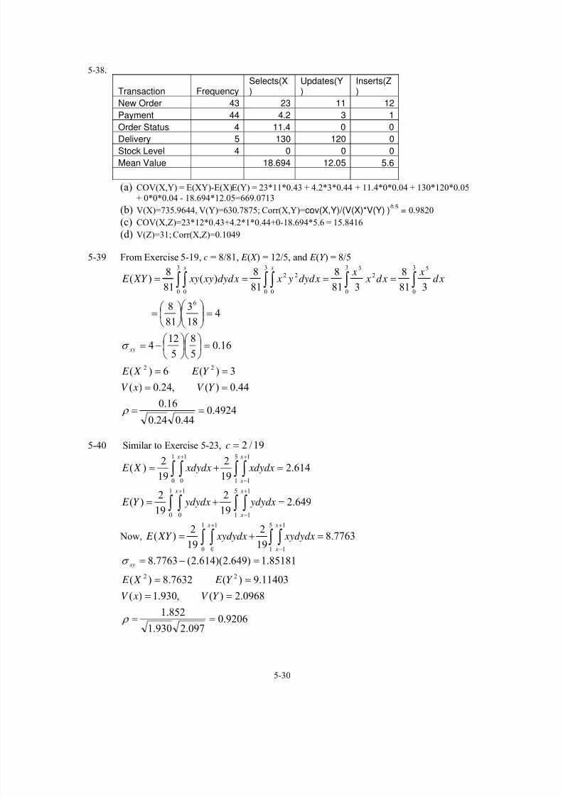
7/12/2019 Solution Manual Stats
http://slidepdf.com/reader/full/solution-manual-stats 105/588
5-30
5-38.
Transaction FrequencySelects(X)
Updates(Y)
Inserts(Z)
New Order 43 23 11 12
Payment 44 4.2 3 1
Order Status 4 11.4 0 0
Delivery 5 130 120 0Stock Level 4 0 0 0
Mean Value 18.694 12.05 5.6
(a) COV(X,Y) = E(XY)-E(X)E(Y) = 23*11*0.43 + 4.2*3*0.44 + 11.4*0*0.04 + 130*120*0.05
+ 0*0*0.04 - 18.694*12.05=669.0713
(b) V(X)=735.9644, V(Y)=630.7875; Corr(X,Y)=cov(X,Y)/(V(X)*V(Y) )0.5
= 0.9820
(c) COV(X,Z)=23*12*0.43+4.2*1*0.44+0-18.694*5.6 = 15.8416
(d) V(Z)=31; Corr(X,Z)=0.1049
5-39 From Exercise 5-19, c = 8/81, E ( X ) = 12/5, and E (Y ) = 8/5
418
3
81
8
3818
3818
818)(
818)(
6
3
0
3
0
3
0
53
0
2
3
0
22
0
=⎟⎟ ⎠
⎞⎜⎜⎝
⎛ ⎟ ⎠
⎞⎜⎝
⎛ =
==== ∫ ∫ ∫∫∫∫ xd x xd x x xdyd y x xdyd xy xy XY E
x x
4924.044.024.0
16.0
44.0)(,24.0)(
3)(6)(
16.05
8
5
124
22
==
==
==
=⎟ ⎠
⎞⎜⎝
⎛ ⎟ ⎠
⎞⎜⎝
⎛ −=
ρ
σ
Y V xV
Y E X E
xy
5-40 Similar to Exercise 5-23, 19/2=c
∫ ∫∫ ∫+
−
+
=+=5
1
1
1
1
0
1
0
614.219
2
19
2)(
x
x
x
xdydx xdydx X E
∫ ∫∫ ∫+
−
+
=+=5
1
1
1
1
0
1
0
649.219
2
19
2)(
x
x
x
ydydx ydydxY E
Now, ∫ ∫∫ ∫+
−
+
=+=5
1
1
1
1
0
1
0
7763.8
19
2
19
2)(
x
x
x
xydydx xydydx XY E
9206.0097.2930.1
852.1
0968.2)(,930.1)(
11403.9)(7632.8)(
85181.1)649.2)(614.2(7763.8
22
==
==
==
=−=
ρ
σ
Y V xV
Y E X E
xy

7/12/2019 Solution Manual Stats
http://slidepdf.com/reader/full/solution-manual-stats 106/588
5-31
5-41 a) E(X) = 1 E(Y) = 1
)()(
)(
00
0 0
Y E X E
dy yedx xe
dxdy xye XY E
y x
y x
=
=
=
∫∫
∫ ∫∞
−∞
−
∞ ∞−−
Therefore, σ ρXY XY= = 0 .
5-42
E(X) = 333.33, E(Y)= 833.33
E(X2)=222,222.2
V(X)=222222.2-(333.33)2=111,113.31
E(Y2)=1,055,556
V(Y)=361,117.11
5547.011.36111731.111113
01.115,111
01.115,111)33.833)(33.333(9.888,388
9.888,388106)(0
002.001.6
==
=−=
=×= ∫ ∫∞ ∞
−−−
ρ
σ xy
x
y xdydx xye XY E
5-43 0)4/1(1)4/1(1)( =+−= X E
0)4/1(1)4/1(1)( =+−=Y E
0(1/4)]1[0+(1/4)]0[1+(1/4)]0[-1+(1/4)]0[-1=E(XY) =××××××××
V(X) = 1/2
V(Y) = 1/2
02/12/1
0
0)0)(0(0
===
=−=
Y X
XY
XY
XY
σ σ
σ
ρ
σ
The correlation is zero, but X and Y are not independent, since, for example, if y = 0, X
must be –1 or 1.
5-44 If X and Y are independent, then )()(),( y f x f y x f Y X XY = and the range of
(X, Y) is rectangular. Therefore,
)()()()()()()( Y E X E dy y yf dx x xf dxdy y f x xyf XY E Y X Y X === ∫∫∫∫
hence σXY=0
5-45 Suppose the correlation between X and Y is ρ. for constants a, b, c, and d, what is the
correlation between the random variables U = aX+b and V = cY+d? Now, E(U) = a E(X) + b and E(V) = c E(Y) + d.
Also, U - E(U) = a[ X - E(X) ] and V - E(V) = c[ Y - E(Y) ]. Then,
XY UV acY E Y X E X acE V E V U E U E σ σ =−−=−−= )]}()][({[)]}()][({[
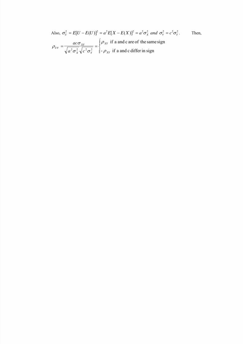
7/12/2019 Solution Manual Stats
http://slidepdf.com/reader/full/solution-manual-stats 107/588
Also,222222222 )]([)]([ Y V X U cand a X E X E aU E U E σ σ σ σ ==−=−= . Then,
⎪
⎪⎨⎧
==signindiffer candaif -
signsametheof arecandaif
2222 XY
XY
Y X
XY
UV
ca
ac
ρ
ρ
σ σ
σ ρ

7/12/2019 Solution Manual Stats
http://slidepdf.com/reader/full/solution-manual-stats 108/588
5-32
Section 5-4
5-46 a)
10
-2
0.00
x0-1
0.01
0.02
0
0.03
0.04
1 2
z(0)
3-10
4y
b)

7/12/2019 Solution Manual Stats
http://slidepdf.com/reader/full/solution-manual-stats 109/588
5-33
10
-2
0.00
x
0.01
0
-1
0.02
0.03
0.04
0
0.05
0.06
0.07
1 2
z(.8)
3-10
4y
c)
10
-2
0.00
x
0.01
0
-1
0.02
0.03
0.04
0
0.05
0.06
0.07
12
z(-.8)
3
-10
4y
5-47 Because 0= ρ and X and Y are normally distributed, X and Y are independent.
Therefore,

7/12/2019 Solution Manual Stats
http://slidepdf.com/reader/full/solution-manual-stats 110/588
5-34
(a) P(2.95 < X < 3.05) = )(04.0
305.304.0
395.2 −− << Z P = 0.7887
(b) P(7.60 < Y < 7.80) = )(08.0
70.780.708.0
70.760.7 −− << Z P = 0.7887
(c) P(2.95 < X < 3.05, 7.60 < Y < 7.80) = P(2.95 < X < 3.05) P(7.60 < Y < 7.80) =
6220.07887.0)()( 2
08.070.780.7
08.070.760.7
04.0305.3
04.0395.2 ==<<<< −−−− Z P Z P
5-48 (a) ρ = cov(X,Y)/σxσy =0.6
cov(X,Y)= 0.6*2*5=6
(b) the marginal probability distribution of X is normal with mean µx , σx.
(c) P(X<116) =P(X-120<-4)=P((X_120)/5<-0.8)=P(Z<-0.8) = 0.21
(d) The conditional probability distribution of X given Y=102 is bivariate normal distribution with
mean and variance
µX|y=102 = 120 – 100*0.6*(5/2) +(5/2)*0.6(102) = 123
σ2X|y=102 = 25(1-0.36) =16
(e) P(X<116|Y=102)=P(Z<(116-123)/4)=0.040
5-49 Because ρ = 0 and X and Y are normally distributed, X and Y are independent.Therefore, μX = 0.1 mm, σX=0.00031 mm, μY = 0.23 mm, σY=0.00017 mm
Probability X is within specification limits is
0.8664)5.1()5.1()5.15.1(
00031.0
1.0100465.0
00031.0
1.0099535.0)100465.0099535.0(
=−<−<=<<−=
⎟ ⎠
⎞⎜⎝
⎛ −<<
−=<<
Z P Z P Z P
Z P X P
Probability that Y is within specification limits is
0.9545)2()2()22(
00017.0
23.023034.0
00017.0
23.022966.0)23034.022966.0(
=−<−<=<<−=
⎟ ⎠
⎞⎜⎝
⎛ −<<
−=<<
Z P Z P Z P
Z P X P
Probability that a randomly selected lamp is within specification limits is(0.8664)(0.9594) = 0.8270
5-50 a) By completing the square in the numerator of the exponent of the bivariate normal PDF, the joint
PDF can be written as
2
)1(2
)1())(((1
2
| 2
2
2
2
2
2
2
1
12
1
)(
),(
⎥⎦
⎤⎢⎣
⎡ −
−
−
⎥⎥
⎦
⎤
⎢⎢
⎣
⎡
⎟⎟ ⎠
⎞⎜⎜⎝
⎛ −−+⎥
⎦
⎤⎢⎣
⎡−+−
−
=
−==
x
x
x
x x
X
Y Y
Y
x
x
x x y
y x
X
XY x X Y
e
e
x f
y x f f
σ
μ
ρ
σ
μ ρ μ
σ
σ ρ μ
σ
σ π
ρ σ πσ
Also, f x(x) =
2
21
2
x
x
x
x
e
μ
σ
π σ
⎡ ⎤−⎢ ⎥⎣ ⎦−
By definition,

7/12/2019 Solution Manual Stats
http://slidepdf.com/reader/full/solution-manual-stats 111/588
5-35
)1(2
))(((1
2
)1(2
)1(2
)1())(((1
2
|
2
2
2
2
2
2
2
2
2
2
12
1
2
1
12
1
)(
),(
ρ−
⎥⎦
⎤⎢⎣
⎡μ−
σ
σρ+μ−
σ−
ρ−
⎥⎦
⎤⎢⎣
⎡
σ
μ−
−
ρ−
⎥⎥
⎦
⎤
⎢⎢
⎣
⎡
⎟⎟ ⎠
⎞⎜⎜⎝
⎛
σ
μ−ρ−+⎥
⎦
⎤⎢⎣
⎡μ−
σ
σρ+μ−
σ−
=
ρ−σπ=
σπ
ρ−σπσ==
x
X
Y Y
Y
x
x
x
x x
X
Y Y
Y
x y
y
x
x
x x y
y x
X
XY x X Y
e
e
e
x f
y x f f
Now f Y|X=x is in the form of a normal distribution.
b) E(Y|X=x) = )( x x
y y x μ−
σ
σρ+μ . This answer can be seen from part a). Since the PDF is in the
form of a normal distribution, then the mean can be obtained from the exponent.
c) V(Y|X=x) = )1( 22 ρ−σ y . This answer can be seen from part a). Since the PDF is in the form of a
normal distribution, then the variance can be obtained from the exponent.
5-51
∫∫
∫ ∫∫ ∫
∞
∞−
⎥⎦
⎤⎢⎣
⎡ −−∞
∞−
⎥⎦
⎤⎢⎣
⎡ −−
∞
∞−
∞
∞−
⎥⎦
⎤⎢⎣
⎡ −+
−−∞
∞−
∞
∞−
⎥
⎥
⎦
⎤
⎢
⎢
⎣
⎡
⎥
⎥
⎦
⎤
⎢
⎢
⎣
⎡
=⎥⎥
⎦
⎤
⎢⎢
⎣
⎡=
dyedxe
dxdyedxdy y x f
Y
Y
Y
X
X
X
Y
Y
X
X
Y X
y x
y x
XY
2
2)(
2
1
2
2)(
2
1
2
2)(
2
2)(
2
1
2
1
2
1
21),(
σ
σ
σ
σ
σ σ σ σ
μ
π
μ
π
μ μ
π
and each of the last two integrals is recognized as the integral of a normal probability
density function from −∞ to ∞. That is, each integral equals one. Since
)()(),( y f x f y x f XY = then X and Y are independent.
5-52 Let )1(2
))((2
2
2
22
12
1),( ρ−
⎥⎥
⎦
⎤
⎢⎢
⎣
⎡
⎟⎟ ⎠
⎞⎜⎜⎝
⎛
σ
μ−+
σσ
μ−μ−ρ−⎟⎟
⎠
⎞⎜⎜⎝
⎛
σ
μ−
−
ρ−σπσ=
Y
Y
Y X
X X
X
X Y Y X X
y x
XY e y x f
Completing the square in the numerator of the exponent we get:
2
2
222
)1())((2
⎟⎟
⎠
⎞
⎜⎜
⎝
⎛ −−+
⎥⎥⎦
⎤
⎢⎢⎣
⎡
⎟⎟ ⎠
⎞⎜⎜⎝
⎛ −−⎟⎟
⎠
⎞⎜⎜⎝
⎛ −=
⎥⎥⎦
⎤
⎢⎢⎣
⎡
⎟⎟ ⎠
⎞⎜⎜⎝
⎛ −+
−−−⎟⎟
⎠
⎞⎜⎜⎝
⎛ −
X
X
X
X
Y
Y
Y
Y
Y X
X X
X
X X X Y Y Y X X
σ
μ ρ
σ
μ ρ
σ
μ
σ
μ
σ σ
μ μ ρ
σ
μ
But,
⎥⎥⎦
⎤
⎢⎢⎣
⎡−+−=
⎥⎥⎦
⎤
⎢⎢⎣
⎡−−−=⎟
⎟
⎠
⎞
⎜⎜
⎝
⎛ −−⎟
⎟
⎠
⎞
⎜⎜
⎝
⎛ −))(((
1)()(
1 x
X
Y Y
Y x
X
Y Y
Y X
X
Y
Y X Y X Y X Y
μ σ
σ ρ μ
σ μ
σ
σ ρ μ
σ σ
μ ρ
σ
μ
Substituting into f XY(x,y), we get

7/12/2019 Solution Manual Stats
http://slidepdf.com/reader/full/solution-manual-stats 112/588
5-36
22
2
2
2
2
2 2 2
1( ( )) (1 )
2(1 )
2
( ( ))
2 (1 )1
2
2
1( , )
2 1
1 1
2 2 1
xY Y x
X xY
y y x
x
x x
x
x y x
XY
x y
y x
x
x y
f x y e dydx
e dx e dy
μ σ μ ρ μ ρ
σ σ σ
ρ
σ μ ρ μ
σ
σ ρ μ
σ
πσ σ ρ
π σ π σ ρ
⎡ ⎤⎛ ⎞⎡ ⎤ −⎢ ⎥− + − + − ⎜ ⎟⎢ ⎥⎢ ⎥⎣ ⎦ ⎝ ⎠⎣ ⎦−∞ ∞ −
−∞ −∞
⎡ ⎤⎛ ⎞⎢ ⎥− + −⎜ ⎟
⎢ ⎥⎝ ⎠−⎢ ⎥⎛ ⎞ −− ⎢ ⎥− ⎜ ⎟ ⎢ ⎥∞ ∞⎝ ⎠ ⎢ ⎥⎣ ⎦
−∞ −∞
=−
= ×−
∫ ∫
∫ ∫
The integrand in the second integral above is in the form of a normally distributed random
variable. By definition of the integral over this function, the second integral is equal to 1:
2
2 2 2
2
( ( ))
2 (1 )1
2
2
1
2
1 1
2 2 1
11
2
y y x
x
x x
x
x
x
y x
x
x y
x
x
e dx e dy
e dx
σ μ ρ μ
σ
σ ρ μ
σ
μ
σ
π σ π σ ρ
π σ
⎡ ⎤⎛ ⎞⎢ ⎥− + −⎜ ⎟⎢ ⎥⎝ ⎠−⎢ ⎥
⎛ ⎞ −− ⎢ ⎥− ⎜ ⎟ ⎢ ⎥∞ ∞⎝ ⎠ ⎢ ⎥⎣ ⎦
−∞ −∞
⎛ ⎞−− ⎜ ⎟∞ ⎝ ⎠
−∞
×−
= ×
∫ ∫
∫
The remaining integral is also the integral of a normally distributed random variable and therefore,
it also integrates to 1, by definition. Therefore,
1),(∫ ∫∞
∞−
∞
∞−= y x f XY
5-53
dyee
dyee
dye x f
X
X
Y
Y
Y
X
X
X
X
X
X
X
Y
Y
Y
X
X
X
Y
Y
Y X
Y X
X
X
Y X
x y x
x x y x
y y x x
X
2
)()(
21
2
2
2)(
2)(
2)()(
21
2
2
2)(
21
2
2)())((
2
2)(
21
2
5.0
12
15.0
2
1
5.0
12
1
5.0
2
1
25.0
12
1)(
⎥⎥⎥
⎦
⎤
⎢⎢⎢
⎣
⎡−
−−−
∞
∞− −
−−
⎪⎭
⎪⎬⎫
⎪⎩
⎪⎨⎧
⎥⎦⎤
⎢⎣⎡ −
−⎥⎦⎤
⎢⎣⎡ −
−−−∞
∞−−
−−
∞
∞−
⎥⎦
⎤⎢⎣
⎡ −+
−−−
−−
−
−
−−
−
∫
∫
∫
=
=
⎥⎥
⎦
⎤
⎢⎢
⎣
⎡=
σ σ
σ
σ
σ
σ σ σ
σ
σ
σ
σ σ σ σ
σ πσ
μ ρ μ
ρ
ρ π
μ
π
μ ρ μ ρ μ
ρ
ρ π
μ
ρ
π
μ μ μ ρ μ
ρ
ρ
The last integral is recognized as the integral of a normal probability density with mean
X
X Y x
Y σ σ
μ μ ρ )( −+ and variance )1( 22
ρ σ −Y . Therefore, the last integral equals one and
the requested result is obtained.Section 5-5

7/12/2019 Solution Manual Stats
http://slidepdf.com/reader/full/solution-manual-stats 113/588
5-54 a) E(2X + 3Y) = 2(0) + 3(10) = 30
b) V(2X + 3Y) = 4V(X) + 9V(Y) = 97
c) 2X + 3Y is normally distributed with mean 30 and variance 97. Therefore,
5.0)0()()3032(97
3030 =<=<=<+ − Z P Z PY X P
d) 8461.0)02.1()()4032( 97
3040
=<=<=<+−
Z P Z PY X P 5-55
(a) E(3X+2Y)= 3*2+2*6=18
(b) V(3X+2Y) = 9*5+4*8 =77
(c) 3X+2Y ~ N( 18, 77)
P(3X+2Y<18) = P(Z<(18-18)/770.5)=0.5
(d) P(3X+2Y<28) = P(Z<(28-18)/770.5)=P(Z<1.1396) =0.873

7/12/2019 Solution Manual Stats
http://slidepdf.com/reader/full/solution-manual-stats 114/588
5-37
5-54 a) E(2X + 3Y) = 2(0) + 3(10) = 30 b) V(2X + 3Y) = 4V(X) + 9V(Y) = 97
c) 2X + 3Y is normally distributed with mean 30 and variance 97. Therefore,
5.0)0()()3032(97
3030 =<=<=<+ − Z P Z PY X P
d) 8461.0)02.1()()4032(97
3040 =<=<=<+ − Z P Z PY X P
5-55
(a) E(3X+2Y)= 3*2+2*6=18
(b) V(3X+2Y) = 9*5+4*8 =77
(c) 3X+2Y ~ N( 18, 77)
P(3X+2Y<18) = P(Z<(18-18)/770.5)=0.5
(d) P(3X+2Y<28) = P(Z<(28-18)/770.5)=P(Z<1.1396) =0.873
Section 5-5
5-56 Y = 10X and E(Y) =10E(X) = 50mm.
V(Y)=102
V(X)=25mm2
5-57 a) Let T denote the total thickness. Then, T = X + Y and E(T) = 4 mm,
V(T) = 0 1 0 1 0 022 2 2. . .+ = mm , and σT = 0 1414. mm.
b)
0170.0983.01)12.2(1
)12.2(1414.0
43.4)3.4(
=−=<−=
>=⎟ ⎠
⎞⎜⎝
⎛ −>=>
Z P
Z P Z PT P
5-58 (a) X: time of wheel throwing. X~N(40,4)
Y : time of wheel firing. Y~N(60,9)
X+Y ~ N(100, 13)
P(X+Y≤ 95) = P(Z<(95-100)/130.5) =P(Z<1.387) =0.917
(b) P(X+Y>110) = 1- P(Z<(110-100)/ 130.5) =1-P(Z<2.774) = 1-0.9972 =0.0028
5-59 a) X ∼ N(0.1, 0.00031) and Y ∼ N(0.23, 0.00017) Let T denote the total thickness.
Then, T = X + Y and E(T) = 0.33 mm,
V(T) =2722 1025.100017.000031.0 mm x
−=+ , and 000354.0=T
σ mm.
0)272(000354.0
33.02337.0)2337.0( ≅−<=⎟
⎠
⎞⎜⎝
⎛ −<=< Z P Z P T P
b)
1)253(1)253(000345.0
33.02405.0)2405.0( ≅<−=−>=⎟
⎠
⎞⎜⎝
⎛ −>=> Z P Z P Z P T P
5-60 Let D denote the width of the casing minus the width of the door. Then, D is normally
distributed.
a) E(D) = 1/8 V(D) =25652
1612
81 )()( =+ 5 0.1398
256T σ = =

7/12/2019 Solution Manual Stats
http://slidepdf.com/reader/full/solution-manual-stats 115/588
5-38
b) 187.0)89.0()()(256
5
8
1
4
1
41 =>=>=>
− Z P Z P DP
c) 187.0)89.0()()0(256
5
8
10
=−<=<=<−
Z P Z P DP
5-61 X : time of ACL reconstruction surgery for high-volume hospitals.
X ~ N(129,196).
E(X1+X2+…+X10) = 10* 129 =1290
V(X1+X2+…+X10) = 100*196 =19600
5-62 a) Let X denote the average fill-volume of 100 cans. 05.01005.0
2
== X
σ .
b) E( X ) = 12.1 and 023.0)2(05.0
1.1212)12( =−<=⎟
⎠
⎞⎜⎝
⎛ −<=< Z P Z P X P
c) P( X < 12) = 0.005 implies that .005.005.0
12=⎟
⎠
⎞⎜⎝
⎛ −<
μ Z P
Then05.0
12 μ −= -2.58 and 129.12=μ .
d) P( X < 12) = 0.005 implies that .005.0100/
1.1212=⎟⎟
⎠
⎞⎜⎜⎝
⎛ −<σ
Z P
Then100/
1.1212
σ
− = -2.58 and 388.0=σ .
e) P( X < 12) = 0.01 implies that .01.0/5.0
1.1212=⎟⎟
⎠
⎞⎜⎜⎝
⎛ −<
n Z P
Thenn/5.0
1.1212− = -2.33 and 13672.135 ≅=n .
5-63 Let X denote the average thickness of 10 wafers. Then, E( X ) = 10 and V( X ) = 0.1.
a) 998.0)16.316.3()()119(1.0
1011
1.0
109 =<<−=<<=<< −− Z P Z P X P .
The answer is 1 − 0.998 = 0.002
b)n X
and X P 101.0)11( ==> σ .
Therefore, 01.0)()11(1
1011 =>=> −
n
Z P X P , 11 101−
n
= 2.33 and n = 5.43 which is
rounded up to 6.
c)10
0005.0)11( σ σ ==> X
and X P .
Therefore, 0005.0)()11(10
1011 =>=> −σ
Z P X P ,10
1011
σ
− = 3.29
9612.029.3/10 ==σ
5-64 X~N(160, 900)
a) Let Y = X1 + X2 + ... + X25, E(Y) = 25E(X) = 4000, V(Y) = 252(900) = 22500
P(Y > 4300) =
0227.09773.01)2(1)2(22500
40004300=−=<−=>=⎟⎟
⎠
⎞⎜⎜⎝
⎛ −> Z P Z P Z P

7/12/2019 Solution Manual Stats
http://slidepdf.com/reader/full/solution-manual-stats 116/588
b) c) P(Y > x) = 0.0001 implies that .0001.022500
4000=⎟⎟
⎠
⎞⎜⎜⎝
⎛ −>x
Z P
Then1504000− x = 3.72 and 4558= x
5-65 W: weights of parts E: measurement error.
W~ N(µw, σw2) , E ~ N(0, σe
2) ,W+E ~ N(µw, σw2+σe
2) .
Wsp = weights of the specification P
(a) P(W > µw + 3σw) + P(W < µw – 3σw) = P(Z > 3) + P(Z < -3) = 0.0027
(b) P(W+E > µw + 3σw) + P( W+E < µw – 3σw)
= P (Z > 3σw / (σw2+σe
2)1/2) + P (Z < -3σw / (σw2+σe
2)1/2)
Because σe2 = 0.5σw
2 the probability is
= P (Z > 3σw / (1.5σw2)1/2) + P (Z < -3σw / (1.5σw
2)1/2)
= P (Z > 2.45) + P (Z < -2.45) = 2(0.0072) = 0.014
No.
(c) P( E + µw + 2σw > µw + 3σw) = P(E > σw) = P(Z > σw/(0.5σw2)1/2)
= P(Z > 1.41) = 0.079
Also, P( E + µw + 2σw < µw – 3σw) = P( E < – 5σw)
= P(Z < -5σw/(0.5σw2)1/2) = P(Z < -7.07) ≈ 0
5-66 D = A - B - C
a) E(D) = 10 - 2 - 2 = 6 mm
mm
mm DV
D 1225.0
015.005.005.01.0)( 2222
=
=++=
σ
b) P(D < 5.9) = P(Z <1225.0
69.5 −) = P(Z < -0.82) = 0.206.

7/12/2019 Solution Manual Stats
http://slidepdf.com/reader/full/solution-manual-stats 117/588
5-39
Section 5-6
5-674
1)( = y f Y at y = 3, 5, 7, 9 from equation 5-40.
5-68 Because X ≥ 0 , the transformation is one-to-one; that is2 x y = and y x = . From equation 5-40,
( y y
y X Y p p y f y f −−== 33 )1()()( for y = 0, 1, 4, 9.
If p = 0.25, ( ) y y
yY y f −= 33 )75.0()25.0()( for y = 0, 1, 4, 9.
5-69 a)72
10
2
1
2
10)(
−=⎟ ⎠
⎞⎜⎝
⎛ ⎟ ⎠
⎞⎜⎝
⎛ −=
y y f y f X Y for 10 ≤ ≤y 22
b) ( ) 1872
1
72
10)(
22
102
10
3
22
10
223
=−=−
= ∫y y
dy y y
Y E
5-70 Because y = -2 ln x, xe y
=−
2 . Then, 222
21
21)()(
y y y
eee f y f X Y
−−−
=−= for ≤≤−
20 y
e 1 or
0≥ y , which is an exponential distribution with λ =1/2 (which equals a chi-square distribution with k = 2
degrees of freedom).

7/12/2019 Solution Manual Stats
http://slidepdf.com/reader/full/solution-manual-stats 118/588
5-71 a) If 2 x y = , then y x = for x ≥ 0 and y ≥ 0 . Thus,
y
e y y f y f
y
X Y 2
)()( 2
1
2
1
−−
== for
y > 0.
b) If 2/1 x y = , then
2 y x = for 0≥ x and 0≥ y . Thus,2
22)()( 2 y
X Y ye y y f y f −== for y >
0.c) If y = ln x, then x ey= for 0≥ x . Thus,
y ye ye y y y
X Y eeeee f y f −− === )()( for
∞<<∞− y .
5-72 a) Now, dveavbv−
∞
∫0
2must equal one. Let u = bv, then 1 .)(
0
2
3
0
2 dueub
a
b
duea uu
b
u −∞
−∞
∫∫ == From
the definition of the gamma function the last expression is33
2)3(
b
a
b
a=Γ . Therefore,
2
3ba = .
b) If 2
2mvw = , then
m
wv
2= for 0,0 ≥≥ wv .
( )
m
w
m
w
b
b
mw
V W
ewmb
mwem
wb
dw
dv f w f
2
2
2/12/33
2/13
2
2
)2(2
2)(
−−
−−
=
==
for 0≥w .
5-73 If xe y = , then x = ln y for 1
21 and 2 e ye x ≤≤≤≤ . Thus, y y
y f y f X Y
11)(ln)( == for
1 2ln ≤≤ y . That is,
y
y f Y 1
)( = for 2e ye ≤≤ .
5-74 If y =2)2( − x , then x = y−2 for 20 ≤≤ x and x = y+2 for 42 ≤≤ x . Thus,
( ) 40for
16
2
16
2
||)2(||)2()(
2/1
4
1
2/1
2
12/1
2
1
≤≤=
++
−=
++−−=
−
−−
y y
y
y
y
y
y y f y y f y f X X Y

7/12/2019 Solution Manual Stats
http://slidepdf.com/reader/full/solution-manual-stats 119/588
5-40
Supplemental Exercises
5-75 The sum of ∑∑ = x y
y x f 1),( , ( ) ( ) ( ) ( ) ( ) 14
14
18
18
14
1 =++++
and 0),( ≥ y x f XY
a) 8/34/18/1)0,0()1,0()5.1,5.0( =+=+=<< XY XY f f Y X P .
b) 4/3)1,1()0,1()1,0()0,0()1( =+++=≤ XY XY XY XY f f f f X P

7/12/2019 Solution Manual Stats
http://slidepdf.com/reader/full/solution-manual-stats 120/588
5-41
c) 4/3)1,1()0,1()1,0()0,0()5.1( =+++=< XY XY XY XY f f f f Y P
d) 8/3)1,1()0,1()5.1,5.0( =+=<> XY XY f f Y X P
e) E(X) = 0(3/8) + 1(3/8) + 2(1/4) = 7/8.
V(X) = 02(3/8) + 12(3/8) + 22(1/4) - 7/82 =39/64
E(Y) = 1(3/8) + 0(3/8) + 2(1/4) = 7/8.
V(Y) = 12
(3/8) + 02
(3/8) + 22
(1/4) - 7/82
=39/64
f) 4 / 1)2(,8 / 3)1(,8 / 3)0(),()( ==== ∑ X X X
y
XY X f f f and y x f x f .
g) 3/2)1(,3/1)0()1(
),1()(
8/3
4/1
18/3
8/1
11=====
Y Y
X
XY
Y f f and
f
y f y f .
h) 3/2)3/2(1)3/1(0)()1|(1
1| =+=== ∑=
= x
X Y y yf X Y E
i) As is discussed after Example 5-19, because the range of (X, Y) is not rectangular, X
and Y are not independent.
j) E( XY ) = 1.25, E( X ) = E(Y )= 0.875 V(X) = V(Y) = 0.6094COV( X ,Y )=E( XY )-E( X )E(Y )= 1.25-0.8752=0.4844
7949.06094.06094.0
4844.0== XY ρ
5-76 a) 0.063170.020.010.0!14!4!2
!20)14,4,2( 1442 ===== Z Y X P
b) 0.121690.010.0)0( 200 ===X P
c) 2)10.0(20)( 1 === np X E
8.1)9.0)(10.0(20)1()( 11==−= pnp X V
d))(
),()19|(|
z f
z x f Z X f
Z
XZ
z Z X ==
z z x x
XZ z x z x
xz f 7.02.01.0)!20(!!
!20)( 20 −−
−−=
z z
Z z z
z f 7.03.0)!20(!
!20)( 20−
−=
z x x
z
z x x
Z
XZ
z Z X z x x
z
z x x
z
z f
z x f Z X f
−−
−
−−
= ⎟ ⎠
⎞⎜⎝
⎛ ⎟ ⎠
⎞⎜⎝
⎛ −−
−=
−−
−==
20
20
20
|3
2
3
1
)!20(!
)!20(
3.0
2.01.0
)!20(!
)!20(
)(
),()19|(
Therefore, X is a binomial random variable with n=20- z and p=1/3. When z=19,
3
2)0(19| = X f and
3
1)1(19| = X f .
e)3
1
3
11
3
20)19|( =⎟
⎠
⎞⎜⎝
⎛ +⎟ ⎠
⎞⎜⎝
⎛ == Z X E
5-77 Let X, Y, and Z denote the number of bolts rated high, moderate, and low. Then, X, Y,
and Z have a multinomial distribution.

7/12/2019 Solution Manual Stats
http://slidepdf.com/reader/full/solution-manual-stats 121/588
5-42
a) 0560.01.03.06.0!2!6!12
!20)2,6,12( 2612 ===== Z Y X P .
b) Because X, Y, and Z are multinomial, the marginal distribution of Z is binomial with
n = 20 and p = 0.1.c) E(Z) = np = 20(0.1) = 2.
d) P(low>2)=1-P(low=0)-P(low=1)-P(low=2)=1-0.1*0.920- 0.1*0.919-0.12*0.918=0.863
e))16(
),16()(
16|
X
XZ Z
f
z f z f = and
z z x x
XZ z x z x
z x f 1.03.06.0)!20(!!
!20),( )20( −−
−−= for
z xand z x ≤≤≤+ 0,020 . Then,
( ) ( ) z z
z z
z z
z z
Z z f
4.01.04
4.03.0
)!4(!!4
416
!4!16!20
)4(16
)!4(!!16!20
164.06.0
1.03.06.0)(
−
−
−− ==
for 40 ≤≤ z . That is the distribution of Z given X = 16 is binomial with n = 4 and
p = 0.25.
f) From part a., E(Z) = 4 (0.25) = 1.
g) Because the conditional distribution of Z given X = 16 does not equal the marginaldistribution of Z, X and Z are not independent.
5-78 Let X, Y, and Z denote the number of calls answered in two rings or less, three or
four rings, and five rings or more, respectively.
a) 0649.005.025.07.0!1!1!8
!10)1,1,8( 118 ===== Z Y X P
b) Let W denote the number of calls answered in four rings or less. Then, W is a binomial
random variable with n = 10 and p = 0.95.
Therefore, P(W = 10) = ( ) 5987.005.095.0 01010
10 = .
c) E(W) = 10(0.95) = 9.5.
d))8(
),8()(
8
X
XZ
Z f
z f z f = and
z z x x
XZ z x z x
z x f 05.025.070.0)!10(!!
!10),( )10( −−
−−= for
z xand z x ≤≤≤+ 0,010 . Then,
( ) ( ) z z
z z
z z
z z
Z z f
30.005.02
30.025.0
)!2(!!2
28
!2!8!10
)2(8
)!2(!!8
!10
830.070.0
05.025.070.0)(
−
−
−− ==
for 0 2≤ ≤z . That is Z is binomial with n =2 and p = 0.05/0.30 = 1/6.
e) E(Z) given X = 8 is 2(1/6) = 1/3.f) Because the conditional distribution of Z given X = 8 does not equal the marginal
distribution of Z, X and Z are not independent.
5-79 ∫ ∫∫ ===3
0
3
03
3
0
2
02
2
2
0
2 18232
ccdxcx ydydxcx x y. Therefore, c = 1/18.
a) ∫ ∫∫ ====<<1
0
108
11
0336
1
1
0
1
02
2
18
1
1
0
2
18
132
)1,1( x ydx x ydydx xY X P

7/12/2019 Solution Manual Stats
http://slidepdf.com/reader/full/solution-manual-stats 122/588
5-43
b) ∫ ∫∫ ====<5.2
0
5.2
039
1
5.2
0
2
02
2
18
1
2
0
2
18
1 5787.0)5.2(32
x ydx x ydydx x X P
c) ∫ ∫∫ ====<<3
0
4
33
0312
1
3
0
2
12
2
18
1
2
1
2
18
132
)5.21( x ydx x ydydx xY P
d)
2199.0
)5.11,2(
432
95
3
2
3
23144
5
3
2
5.1
12
2
18
1
5.1
1
2
18
132
==
===<<> ∫ ∫∫ x ydx x ydydx xY X P
e) ∫ ∫∫ ====3
0
4
93
049
1
3
0
3
18
1
2
0
3
18
14
2)( xdx x ydydx x X E
f) ∫ ∫∫ ====3
0
3
43
0327
4
3
0
3
82
18
1
2
0
22
18
13
)( xdx xdydx y xY E
g) 30)( 2
9
1
2
0
2
18
1 <<== ∫ x for x ydy x x f X
h)2)1(
),1()(
9
1
18
1 y y
f
y f y f
X
XY
X Y === for 0 < y < 2.
i))1()1(
)1,()(
2
18
1
1
Y Y
XY
X f
x
f
x f x f == and 20)(
2
3
0
2
18
1 <<== ∫ y for ydx x y f y
Y .
Therefore,2
9
1
2
18
1
12/1
)( x x
x f X
== for 0 < x < 3.
5-80 The region x y2 2 1+ ≤ and 0 < z < 4 is a cylinder of radius 1 ( and base area π ) and
height 4. Therefore, the volume of the cylinder is 4π and f x y zXYZ( , , ) =1
4πfor x y2 2 1+ ≤
and 0 < z < 4.
a) The region X Y2 2 0 5+ ≤ . is a cylinder of radius 0 5. and height 4. Therefore,
2/1)5.0(4
)5.0(422 ==≤+π
π Y X P .
b) The region X Y2 2 0 5+ ≤ . and 0 < z < 2 is a cylinder of radius 0 5. and height 2.
Therefore,
4/1)2,5.0( 4
)5.0(222
==<≤+ π
π
Z Y X P
c))1(
)1,,(),(
1
Z
XYZ
XY f
y x f y x f = and 4/1)(
1
41
22
== ∫∫≤+
dydx z f
y x
Z π
for 0 < z < 4. Then, 14/1
4/1),( 221
1≤+== y x for y x f
XY π
π .

7/12/2019 Solution Manual Stats
http://slidepdf.com/reader/full/solution-manual-stats 123/588
5-44
d)222
4
0
21
41
1
1
4
0
11)(
2
2
xdz xdydz x f
x
x
X −=−== ∫∫∫−
−−
π π π for -1 < x < 1
e)
)0,0(
),0,0()(
0,0
XY
XYZ
Z
f
z f z f = and π
π
/1),(4
0 4
1 ==
∫dz y x f XY for 122 ≤+ y x . Then,
4/1/1
4/1)(
0,0==
π
π z f
Z for 0 < z < 4 and 2
0,0=
Z μ .
f) 4/1/1
4/1
),(
),,()( ===
π
π
y x f
z y x f z f
XY
XYZ
xy Z for 0 < z < 4. Then, E(Z) given X = x and Y = y is
24
0
4=∫ dz z
.
5-81 c y x f XY =),( for 0 < x < 1 and 0 < y < 1. Then,
∫∫=
1
0
1
0
1cdxdy and c = 1. Because
),( y x f XY is constant, )5.0( <− Y X P is the area of the shaded region below
0
0.5
0.5
1
1
That is, )5.0( <− Y X P = 3/4.
5-82 a) Let X X X1 2 6, ,..., denote the lifetimes of the six components, respectively. Because of
independence,P X X X P X P X P X( , , . .. , ) ( ) ( )... ( )1 2 6 1 2 65000 5000 5000 5000 5000 5000> > > = > > >
If X is exponentially distributed with mean θ , then λθ
= 1 and
θ θ θ
θ
///1)( x
x
t
x
t eedt e x X P
−∞
−∞
− =−==> ∫ . Therefore, the answer is
0978.0325.22.025.025.05.05.08/5
==−−−−−−−
eeeeeee . b) The probability that at least one component lifetime exceeds 25,000 hours is
the same as 1 minus the probability that none of the component lifetimes exceed
25,000 hours. Thus,
1-P(Xa<25,000, X2<25,000, …, X6<25,000)=1-P(X1<25,000)…P(X6<25,000)
=1-(1-e-25/8
)(1-e-2.5
)(1-e-2.5
)(1-e-1.25
)(1-e-1.25
)(1-e-1
)=1-.2592=0.7408

7/12/2019 Solution Manual Stats
http://slidepdf.com/reader/full/solution-manual-stats 124/588
5-45
5-83 Let X, Y, and Z denote the number of problems that result in functional, minor, and no
defects, respectively.
a) 085.03.05.02.0)3,5,2()5,2( 352
!3!5!2
!10 ======== Z Y X PY X P
b) Z is binomial with n = 10 and p = 0.3.c) E(Z) = 10(0.3) = 3.
5-84 a) Let X denote the mean weight of the 25 bricks in the sample. Then, E( X ) = 3 and
05.025
25.0 == X
σ . Then, P( X < 2.95) = P(Z < 2 95 30 05.
.− ) = P (Z < -1) = 0.159.
b) 99.0)05.
3()( =
−>=>
x Z P x X P . So, =
−05.0
3 x-2.33 and x=2.8835.
5-85 a)
Because ,25.025.5
75.4
25.18
75.17
ccdydx =∫∫ c = 4. The area of a panel is XY and P(XY > 90) is the
shaded area times 4 below,
5.25
4.75
17.25 18.25
That is, 499.0)ln9025.5(425.54425.18
75.17
25.18
75.17
90
25.5
/90
25.18
75.17
=−=−= ∫∫∫ x xdxdydx x
x
b) The perimeter of a panel is 2X+2Y and we want P(2X+2Y >46)
5.0)2
75.17(4)75.17(4
)23(25.544
25.18
75.17
225.18
75.17
25.18
75.17
25.5
23
25.18
75.17
=+−=+−=
−−=
∫
∫∫∫−
x xdx x
dx xdydx x
5-86 a) Let X denote the weight of a piece of candy and X∼ N(0.1, 0.01). Each package has 16
candies, then P is the total weight of the package with 16 pieces and E( P ) = 16(0.1)=1.6ounces and V(P) = 162(0.012)=0.0256 ounces2
b) 5.0)0()()6.1(16.0
6.16.1 =<=<=< − Z P Z PPP .
c) Let Y equal the total weight of the package with 17 pieces, E(Y) = 17(0.1)=1.7 ounces
and V(Y) = 172(0.012)=0.0289 ounces2
2776.0)59.0()()6.1(0289.0
7.16.1 =−<=<=< − Z P Z PY P .
5-87 Let X denote the average time to locate 10 parts. Then, E( X ) =45 and10
30= X
σ
a) 057.0)58.1()()60(10/30
4560 =>=>=> − Z P Z P X P

7/12/2019 Solution Manual Stats
http://slidepdf.com/reader/full/solution-manual-stats 125/588
5-46
b) Let Y denote the total time to locate 10 parts. Then, Y > 600 if and only if X > 60.
Therefore, the answer is the same as part a.
5-88 a) Let Y denote the weight of an assembly. Then, E(Y) = 4 + 5.5 + 10 + 8 = 27.5 and
V(Y)= 7.05.02.05.04.0 2222 =+++ .
0084.0)39.2()()5.29( 7.0
5.275.29
=>=>=>−
Z P Z PY P b) Let X denote the mean weight of 8 independent assemblies. Then, E( X ) = 27.5 and
V( X ) = 0.7/8 = 0.0875. Also, 0)07.5()()29(0875.0
5.2729 =>=>=> − Z P Z P X P .
5-89
10
-2
0.00
x
0.01
0
-1
0.02
0.03
0.04
0
0.05
0.06
0.07
1 2
z(-.8)
3-10
4y
5-90
⎥⎥⎦
⎤
⎢⎢⎣
⎡−+−−−−
−
−
⎥⎦
⎤⎢⎣
⎡−+−−−−
−
⎥⎦
⎤⎢⎣
⎡ −+−−−−−
−=
=
=
})2()2)(1)(8(.2)1{()8.01(2
1
2
})2()2)(1(6.1)1{()36.0(2
1
})2()2)(1(6.1)1{(72.0
1
22
2
22
22
8.12
1),(
36.2
1),(
2.1
1),(
y y x x
XY
y y x x
XY
y y x x
XY
e y x f
e y x f
e y x f
π
π
π
1)( = X E , 2)( =Y E 1)( = X V 1)( =Y V and ρ = 0.8
5-91 Let T denote the total thickness. Then, T = X1 + X2 anda) E(T) = 0.5+1=1.5 mm

7/12/2019 Solution Manual Stats
http://slidepdf.com/reader/full/solution-manual-stats 126/588
a. V(T)=V(X1) +V(X2) + 2Cov(X1X2)=0.01+0.04+2(0.014)=0.078mm2
i. where Cov(XY)=ρσXσY=0.7(0.1)(0.2)=0.014
b) 0367.0)79.1(078.0
5.11)1( =−<=⎟⎟
⎠
⎞⎜⎜⎝
⎛ −<=< Z P Z PT P
c) Let P denote the total thickness. Then, P = 2X1 +3 X2 andE(P) =2(0.5)+3(1)=4 mm
V(P)=4V(X1) +9V(X2) +
2(2)(3)Cov(X1X2)=4(0.01)+9(0.04)+2(2)(3)(0.014)=0.568mm2
where Cov(XY)=ρσXσY=0.7(0.1)(0.2)=0.014
5-92 Let T denote the total thickness. Then, T = X1 + X2 + X3 anda) E(T) = 0.5+1+1.5 =3 mm
V(T)=V(X1) +V(X2) +V(X3)+2Cov(X1X2)+ 2Cov(X2X3)+
2Cov(X1X3)=0.01+0.04+0.09+2(0.014)+2(0.03)+ 2(0.009)=0.246mm2
where Cov(XY)=ρσXσY
b) 0)10.6(246.0
35.1)5.1( ≅−<=⎟
⎠ ⎞⎜
⎝ ⎛ −<=< Z P Z PT P
5-93 Let X and Y denote the percentage returns for security one and two respectively.
If ½ of the total dollars is invested in each then ½X+ ½Y is the percentage return.
E(½X+ ½Y) = 0.05 (or 5 if given in terms of percent)V(½X+ ½Y) = 1/4 V(X)+1/4V(Y)+2(1/2)(1/2)Cov(X,Y)
where Cov(XY)=ρσXσY=-0.5(2)(4) = -4
V(½X+ ½Y) = 1/4(4)+1/4(6)-2 = 3Also, E(X) = 5 and V(X) = 4. Therefore, the strategy that splits between the securities
has a lower standard deviation of percentage return than investing 2million in the first
security.
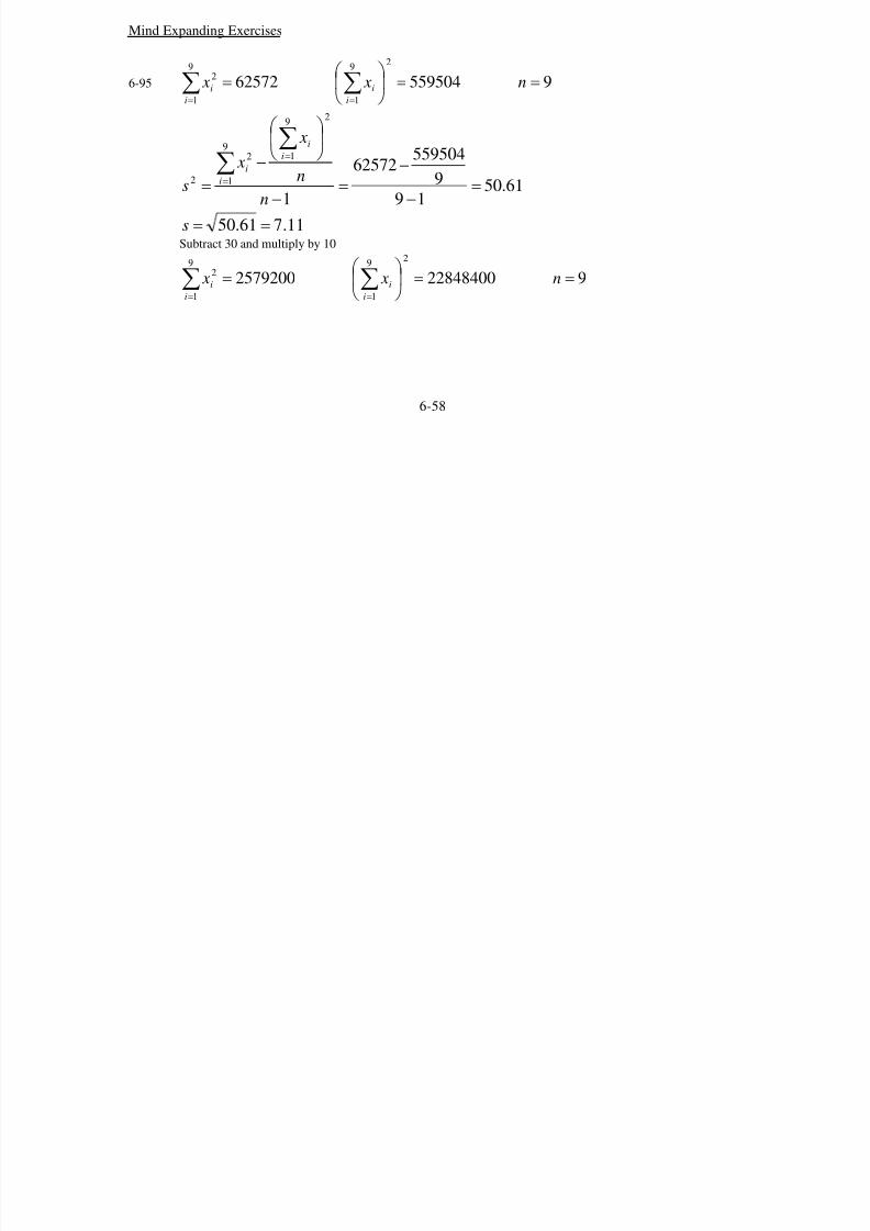
7/12/2019 Solution Manual Stats
http://slidepdf.com/reader/full/solution-manual-stats 127/588
Mind Expanding Exercises
6-95 955950462572
29
1
9
1
2 ==⎟ ⎠
⎞⎜⎝
⎛ = ∑∑
==
n x xi
i
i
i
11.761.50
61.5019
9
55950425726
1
29
19
1
2
2
==
=−
−=
−
⎟ ⎠
⎞⎜⎝
⎛
−=
∑∑ =
=
s
n
n
x
x
s
i
i
i
i
Subtract 30 and multiply by 10
9228484002579200
29
1
9
1
2 ==⎟ ⎠
⎞⎜⎝
⎛ = ∑∑
==
n x xi
i
i
i
6-58

7/12/2019 Solution Manual Stats
http://slidepdf.com/reader/full/solution-manual-stats 128/588
14.711.5061
1.506119
9
228484005792002
1
29
19
1
2
2
==
=−
−=
−
⎟ ⎠
⎞⎜⎝
⎛
−=
∑∑ =
=
s
n
n
x
x
s
i
i
i
i
Yes, the rescaling is by a factor of 10. Therefore, s2 and s would be rescaled by multiplying s2 by 102
(resulting in 5061.1) and s by 10 (71.14). Subtracting 30 from each value has no affect on the variance or
standard deviation. This is because .)()( 2 X V abaX V =+
6-962
1
2
1
2 )()()( a xn x xa xn
i
i
n
i
i −+−=− ∑∑==
; The sum written in this form shows that the quantity is
minimized when a = x .
6-97 Of the two quantities ( )∑=
−n
i
i x x1
2and , the quantity(∑
=
−n
i
i x1
2μ ) (∑
=
−n
i
i x x1
2) will be smaller
given that μ ≠ x . This is because x is based on the values of the ’s. The value of μ may be quite
different for this sample.
i x
6-98 ii bxa y +=
n
x
x
n
i
i∑== 1
and xban
xbna
n
bxa
y
n
i
i
n
i
i
+=+
=+
=∑∑== 11
)(
( )
1
1
2
2
−
−=∑=
n
x x
s
n
i
i
x and2
x x ss =
221
22
1
2
1
2
2
1
)(
1
)(
1
)(
x
n
i
i
n
i
i
n
i
i
y sbn
x xb
n
xbbx
n
xbabxa
s =−
−=
−
−=
−
−−+=
∑∑∑===
Therefore, x y bss =
6-99 00.835= x °F °F5.10= xs
The results in °C:
6-59
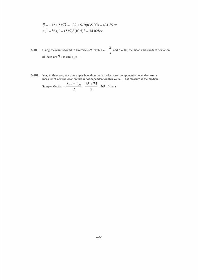
7/12/2019 Solution Manual Stats
http://slidepdf.com/reader/full/solution-manual-stats 129/588
89.431)00.835(9 / 5329 / 532 =+−=+−= x y °C
028.34)5.10()9 / 5( 22222 === x y sbs °C
6-100. Using the results found in Exercise 6-98 with a =s x− and b = 1/ s, the mean and standard deviation
of the zi are z = 0 and sZ = 1.
6-101. Yes, in this case, since no upper bound on the last electronic component is available, use a
measure of central location that is not dependent on this value. That measure is the median.
Sample Median = hours x x
692
7563
2
)5()4( =+
=+
6-60
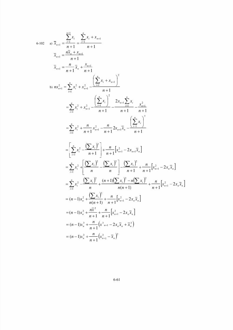
7/12/2019 Solution Manual Stats
http://slidepdf.com/reader/full/solution-manual-stats 130/588
6-102 a)11
1
1
1
1
1 +
+=
+=
∑∑=
+
+
=+
n
x x
n
x
x
n
i
ni
n
i
i
n
1
1
1 +
+
=
+
+ n
x xn
x
nn
n
11
1
1 ++
+= +
+n
x x
n
n x n
nn
b)1
2
1
12
1
1
22
1 +
⎟ ⎠
⎞⎜⎝
⎛ +
−+=+
=+
=+
∑∑
n
x x
x xns
n
n
i
i
n
n
i
in
( )[ ]
( ) ( ) ( )[ ]
( ) ( ) ( )[ ]
( )[ ]
[ ]
( )
( )2
1
22
21
22
2
1
22
2
1
2
2
2
1
222
1
2
2
1
222
1
2
1
2
1
1
2
2
2
1
1
1
2
1
2
2
11
1
2
1
1
2
1
2
1)1(
21
)1(
211
)1(
21)1(
)1(
21)1(
)1(
2
11
211
12
11
11
2
1
nnn
nnnnn
nnnn
nnn
i
n
nnn
iiin
i
i
nnn
iiin
i
i
nnn
n
i
i
i
n
i
i
nn
n
i
ni
n
n
i
in
n
i
in
i
ni
x xn
nsn
x x x xn
nsn
x x xn
n
n
xnsn
x x xn
n
nn
xsn
x x xn
n
nn
xn xn
n
x x
x x x
n
n
n
x
n
x
n
x x
x x xn
n
n
x x
n
x
x xn
n x
n
n x
n
x
n
x x
n
x
x x
−+
+−=
+−+
+−=
−+
++
+−=
−+
++
+−=
−+
++
−++−=
−
+
+
+
−
⎥
⎥
⎦
⎤
⎢
⎢
⎣
⎡−+=
−+
+⎥⎥⎦
⎤
⎢⎢⎣
⎡
+−=
+
⎟ ⎠
⎞⎜⎝
⎛
−+
−+
+=
+−
+−
+
⎟ ⎠
⎞⎜⎝
⎛
−+=
+
+
+
+
+=
+=
++=
=+
=+
+=+
=
=+
∑
∑∑∑∑
∑∑∑
∑
∑ ∑
∑∑
∑∑∑
6-61

7/12/2019 Solution Manual Stats
http://slidepdf.com/reader/full/solution-manual-stats 131/588
c) 65.811=n x inches 641 =+n x
37435.42 == nsn 2.106=ns
098.2
37
)811.6564(137
37435.4)137(
76.65137
64)81.65(37
2
1
1
=
−+
+−=
=+
+=
+
+
n
n
s
x
6-103. The trimmed mean is pulled toward the median by eliminating outliers.
a) 10% Trimmed Mean = 89.29
b) 20% Trimmed Mean = 89.19
Difference is very small
c) No, the differences are very small, due to a very large data set with no significant outliers.
6-104. If nT/100 is not an integer, calculate the two surrounding integer values and interpolate between the two.
For example, if nT/100 = 2/3, one could calculate the mean after trimming 2 and 3 observations from each
end and then interpolate between these two means.
6-62

7/12/2019 Solution Manual Stats
http://slidepdf.com/reader/full/solution-manual-stats 132/588
CHAPTER 6
Section 6-1
6-1. Sample average:
mm0044.748
035.5921 ===∑
=
n
x
x
n
i
i
Sample variance:
( )
2
2
2
1
1
2
2
8
1
2
8
1
)mm(000022414.07
0001569.0
18
8
035.59218031.43813
1
03118.43813
035.592
==
−
−=
−
⎟ ⎠
⎞⎜⎝
⎛
−
=
=
=
∑∑
∑
∑
=
=
=
=
n
n
x
x
s
x
x
n
i
in
i
i
i
i
i
i
Sample standard deviation:
mm00473.0000022414.0 ==s
The sample standard deviation could also be found using
( )s
x x
n
ii
n
=
−
−=∑
2
1
1where ( )x xi
i
− ==∑
2
1
8
0 0001569.
Dot Diagram:
.. ...: .
-------+---------+---------+---------+---------+---------diameter
73.9920 74.0000 74.0080 74.0160 74.0240 74.0320
There appears to be a possible outlier in the data set.
6-1

7/12/2019 Solution Manual Stats
http://slidepdf.com/reader/full/solution-manual-stats 133/588
6-2. Sample average:
min359.1419
82.272
19
19
1 ===∑
=ii x
x
Sample variance:
( )
2
2
2
1
1
2
2
19
1
2
19
1
(min)47.35618
49.6416
119
19
82.2728964.10333
1
8964.10333
82.272
==
−
−=
−
⎟ ⎠
⎞⎜⎝
⎛
−
=
=
=
∑∑
∑
∑
=
=
=
=
n
n
x
x
s
x
x
n
i
in
i
i
i
i
i
i
Sample standard deviation:
min88.1847.356 ==s
The sample standard deviation could also be found using
( )s
x x
n
ii
n
=
−
−=∑
2
1
1
where
( ) 49.641619
1
2 =−∑=i
i x x
6-2

7/12/2019 Solution Manual Stats
http://slidepdf.com/reader/full/solution-manual-stats 134/588
6-3. Sample average:
yards x 1.706812
84817==
Sample variance:
( )
( )
2
2
2
1
1
2
2
19
1
2
12
1
265.5130211
92.564324
112
12
84817600057949
1
600057949
84817
yards
n
n
x
x
s
x
x
n
i
in
i
i
i
i
i
i
==
−
−=
−
⎟ ⎠
⎞⎜⎝
⎛
−
=
=
=
∑∑
∑
∑
=
=
=
=
Sample standard deviation:
yardss 5.226265.51302 ==
The sample standard deviation could also be found using
( )
1
1
2
−
−
=∑
=
n
x x
s
n
i
i
where
( ) 92.56432412
1
2 =−∑=i
i x x
Dot Diagram: (rounding was used to create the dot diagram)
. . : .. .. : :
-+---------+---------+---------+---------+---------+-----C1
6750 6900 7050 7200 7350 7500
6-3

7/12/2019 Solution Manual Stats
http://slidepdf.com/reader/full/solution-manual-stats 135/588
6-4. Sample mean:
kN22.12618
2272
18
18
1 ===∑
=ii x
x
Sample variance:
( )
2
2
2
1
1
2
2
18
1
2
18
1
)kN(24.68317
11.11615
118
18
2272298392
1
298392
2272
==
−
−=
−
⎟ ⎠
⎞⎜⎝
⎛
−
=
=
=
∑∑
∑
∑
=
=
=
=
n
n
x
x
s
x
x
n
i
in
i
i
i
i
i
i
Sample standard deviation:
kN14.2624.683 ==s
The sample standard deviation could also be found using
( )
1
1
2
−
−
=∑
=
n
x x
s
n
i
i
where
( ) 11.1161518
1
2 =−∑=i
i x x
Dot Diagram:
.
: :: . :: . . : . .
+---------+---------+---------+---------+---------+-------yield
90 105 120 135 150 165
6-4

7/12/2019 Solution Manual Stats
http://slidepdf.com/reader/full/solution-manual-stats 136/588
6-5. Sample average:
975.438
8.351== x
Sample variance:
( )
143.1517
998.1057
18
8
8.351043.16528
1
403.16528
8.351
2
2
1
1
2
2
19
1
2
8
1
==
−
−=
−
⎟ ⎠
⎞⎜⎝
⎛
−
=
=
=
∑∑
∑
∑
=
=
=
=
n
n
x
x
s
x
x
n
i
in
i
i
i
i
i
i
Sample standard deviation:
294.12143.151 ==s
The sample standard deviation could also be found using
( )
1
1
2
−
−
=∑
=
n
x x
s
n
i
i
where
( ) 998.10578
1
2=−∑
=ii x x
Dot Diagram:
. . .. . .. .
+---------+---------+---------+---------+---------+-------
24.0 32.0 40.0 48.0 56.0 64.0
6-5

7/12/2019 Solution Manual Stats
http://slidepdf.com/reader/full/solution-manual-stats 137/588
6-6. Sample average:
2
35
1 / 514.81035
28368
35mwatts
x
x i
i
===∑
=
Sample variance:
( )
22
2
2
1
1
2
2
19
1
2
19
1
) / (61.16465
34
743.559830
135
35
2836823552500
1
23552500
28368
mwatts
n
n
x
x
s
x
x
n
i
in
i
i
i
i
i
i
=
=−
−=
−
⎟ ⎠
⎞⎜⎝
⎛
−
=
=
=
∑∑
∑
∑
=
=
=
=
Sample standard deviation:2 / 32.12861.16465 mwattss ==
The sample standard deviation could also be found using
( )
1
1
2
−
−
=∑
=
n
x x
s
n
i
i
where
( ) 743.55983035
1
2 =−∑=i
i x x
Dot Diagram (rounding of the data is used to create the dot diagram)
x
. .
. : .: ... . . .: :. . .:. .:: :::
-----+---------+---------+---------+---------+---------+-x
500 600 700 800 900 1000
The sample mean is the point at which the data would balance if it were on a scale.
6-7. 44.512706905 ==μ ; The value 5.44 is the population mean since the actual physical population
of all flight times during the operation is available.
6-8. Sample average:
6-6

7/12/2019 Solution Manual Stats
http://slidepdf.com/reader/full/solution-manual-stats 138/588
mmn
x
x
n
i
i
173.29
56.191 ===∑
=
Sample variance:
( )
2
2
2
1
1
2
2
9
1
2
9
1
)(4303.0
8
443.3
19
9
56.19953.45
1
953.45
56.19
mm
n
n
x
x
s
x
x
n
i
in
i
i
i
i
ii
=
=−
−=
−
⎟ ⎠
⎞⎜⎝
⎛
−
=
=
=
∑∑
∑∑
=
=
=
=
Sample standard deviation:
mms 6560.04303.0 ==
Dot Diagram . . . . . . . ..
-------+---------+---------+---------+---------+---------crack length
1.40 1.75 2.10 2.45 2.80 3.15
6-9. Sample average of exercise group:
89.28712
3454.681 ===∑
=
n
x
x
n
i
i
Sample variance of exercise group:
112
12
)68.3454(54.1118521
1s
1118521.54
68.3454
2
2
1
1
2
2
1
2
1
−
−=
−
⎟ ⎠
⎞⎜⎝
⎛
−
=
=
=
∑∑
∑
∑
=
=
=
=
n
n
x
x
x
x
n
i
in
i
i
n
i
i
n
i
i
11268.5211
123953.71==
6-7

7/12/2019 Solution Manual Stats
http://slidepdf.com/reader/full/solution-manual-stats 139/588
Sample standard deviation of exercise group:
15.10652.11268 ==s
Dot Diagram of exercise group:
6 h o u r s o f E x e r c i s e
4 5 04 0 03 5 03 0 02 5 02 0 01 5 0
D o t p l o t o f 6 h o u r s o f E x e r c i s e
Sample average of no exercise group:
325.0108
2600.081 ===∑
=
n
x
x
n
i
i
Sample variance of no exercise group:
18
8
)08.2600(947873.4
1s
947873.4
08.2600
2
2
1
1
2
2
1
2
1
−
−=
−
⎟ ⎠
⎞⎜⎝
⎛
−
=
=
=
∑∑
∑
∑
=
=
=
=
n
n
x
x
x
x
n
i
in
i
i
n
i
i
n
i
i
14688.777
102821.4==
Sample standard deviation of no exercise group:
20.12177.14688 ==s
Dot Diagram of no exercise group:
6-8

7/12/2019 Solution Manual Stats
http://slidepdf.com/reader/full/solution-manual-stats 140/588
N o E x e r c i s e
5 0 04 5 04 0 03 5 03 0 02 5 02 0 01 5 0
D o t p l o t o f N o E x e r c i s e
6-10. Dot Diagram of CRT data in exercise 6-5 (Data were rounded for the plot)
70605040302010
Dotplot for Exp 1-Exp 2
Exp 1
Exp 2
The data are centered a lot lower in the second experiment. The lower CRT resolution reduces thevisual accommodation.
6-11. 184.78
47.571 ===∑
=
n
x
x
n
i
i
( )
000427.07
00299.0
18
8
47.57853.412
1
2
2
1
1
2
2 ==−
−=
−
⎟ ⎠
⎞⎜⎝
⎛
−
=
∑∑ =
=
n
n
x
x
s
n
i
in
i
i
02066.0000427.0 ==s
Examples: repeatability of the test equipment, time lag between samples, during which the pH of
the solution could change, and operator skill in drawing the sample or using the instrument.
6-12. sample mean 11.839
0.7481 ===∑
=
n
x
x
n
i
i
drag counts
6-9

7/12/2019 Solution Manual Stats
http://slidepdf.com/reader/full/solution-manual-stats 141/588
sample variance
( )
2
2
2
1
1
2
2
countsdrag61.508
89.404
19
9
0.74862572
1
==
−
−=
−
⎟ ⎠
⎞⎜⎝
⎛
−
=
∑∑ =
=
n
n
x
x
s
n
i
in
i
i
sample standard deviation 11.761.50 ==s drag counts
Dot Diagram
. . . . . . . . .
---+---------+---------+---------+---------+---------+---drag counts
75.0 80.0 85.0 90.0 95.0 100.0
6-13. a) 86.65= x °F
°F 16.12=s
Dot Diagram: :
. . . . .. .: .: . .:..: .. :: .... ..
-+---------+---------+---------+---------+---------+-----temp
30 40 50 60 70 80
b) Removing the smallest observation (31), the sample mean and standard deviation become
86.66= x °F s = 10.74 °F

7/12/2019 Solution Manual Stats
http://slidepdf.com/reader/full/solution-manual-stats 142/588
Section 6-2
6-14.
NOTE: The data set contains one additional measurement of 91.2 that should be included in the
book. Solutions use this additional measurement.
Stem-and-leaf display of octane rating N = 82
Leaf Unit = 0.10 83|4 represents 83.4
1 83|4
3 84|33
4 85|37 86|777
13 87|456789
24 88|23334556679
34 89|0233678899
(13) 90|0111344456789
36 91|00011122256688
22 92|22236777
14 93|023347
8 94|2247
4 95|
4 96|15
2 97|
2 98|8
1 99|
1 100|3
6-10

7/12/2019 Solution Manual Stats
http://slidepdf.com/reader/full/solution-manual-stats 143/588
Median = 90.4, Q1 = 88.6 , and Q3 = 92.2
6-15. Stem-and-leaf display for cycles to failure: unit = 100 1|2 represents 1200
1 0T|3
1 0F|
5 0S|777710 0o|88899
22 1*|000000011111
33 1T|22222223333
(15) 1F|444445555555555
22 1S|66667777777
11 1o|888899
5 2*|011
2 2T|22
Median = 1436.5, Q1 = 1097.8, and Q3 = 1735.0
No, only 5 out of 70 coupons survived beyond 2000 cycles.
6-16. Stem-and-leaf display of percentage of cotton N = 64
Leaf Unit = 0.10 32|1 represents 32.1%
1 32|1
6 32|56789
9 33|114
17 33|56666688
24 34|0111223
(14) 34|55666667777779
26 35|001112344
17 35|56789
12 36|234
9 36|6888
5 37|13
3 37|689
Median = 34.7, Q1 = 33.800 , and Q3 = 35.575
6-17. Stem-and-leaf display for Problem 2-4.yield: unit = 1 1|2 represents 12
1 7o|8
1 8*|
7 8T|223333
21 8F|44444444555555
38 8S|66666666667777777
(11) 8o|88888999999
41 9*|00000000001111
27 9T|22233333
19 9F|444444445555
7 9S|666677
1 9o|8
Median = 89.250, Q1 = 86.100, and Q3 = 93.125
6-18. The data in the 42nd is 90.4 which is median.
The mode is the most frequently occurring data value. There are several data values that occur 3
times. These are: 86.7, 88.3, 90.1, 90.4, 91, 91.1, 91.2, 92.2, and 92.7, so this data set has a
multimodal distribution.
6-11

7/12/2019 Solution Manual Stats
http://slidepdf.com/reader/full/solution-manual-stats 144/588
Sample mean: 534.9083
7514.31 ===∑=
n
x
x
n
i
i
6-19.
Sample median is at( )
2
170 += 35.5th , the median is 1436.5.
Modes are 1102, 1315, and 1750 which are the most frequent data.
Sample mean: 7.140370
982591 ===∑=
n
x
x
n
i
i
6-20.
Sample median is at( )
2
164 += 32.5th
The 32nd is 34.7 and the 33rd is 34.7, so the median is 34.7.
Mode is 34.7 which is the most frequent data.
Sample mean: 798.3464
2227.11 ===∑=
n
x
x
n
i
i
6-21.Stem-and-leaf of Billion of kilowatt hours N = 23
Leaf Unit = 100
(18) 0 000000000000000111
5 0 23
3 0 5
2 0
2 0 9
1 1
1 1
1 1
1 1 6
Sample median is at 12th = 38.43.
Sample mean: 0.19123
8.43981 ===∑=
n
x
x
n
i
i
Sample variance: s2 = 150673.8
Sample standard deviation: s = 388.2
6-12
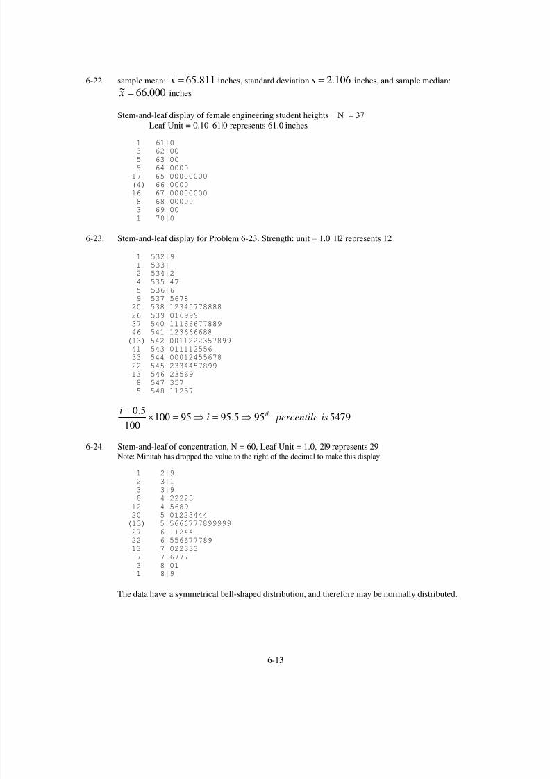
7/12/2019 Solution Manual Stats
http://slidepdf.com/reader/full/solution-manual-stats 145/588
6-22. sample mean: 65.811= x inches, standard deviation 2.106=s inches, and sample median:
66.000~ = x inches
Stem-and-leaf display of female engineering student heights N = 37
Leaf Unit = 0.10 61|0 represents 61.0 inches
1 61|0
3 62|00
5 63|00
9 64|0000
17 65|00000000
(4) 66|0000
16 67|00000000
8 68|00000
3 69|00
1 70|0
6-23. Stem-and-leaf display for Problem 6-23. Strength: unit = 1.0 1|2 represents 12
1 532|9
1 533|2 534|2
4 535|47
5 536|6
9 537|5678
20 538|12345778888
26 539|016999
37 540|11166677889
46 541|123666688
(13) 542|0011222357899
41 543|011112556
33 544|00012455678
22 545|2334457899
13 546|23569
8 547|357
5 548|11257
5479955.9595100100
5.0is percentilei
i th⇒=⇒=×−
6-24. Stem-and-leaf of concentration, N = 60, Leaf Unit = 1.0, 2|9 represents 29Note: Minitab has dropped the value to the right of the decimal to make this display.
1 2|9
2 3|1
3 3|9
8 4|22223
12 4|5689
20 5|01223444
(13) 5|5666777899999
27 6|11244
22 6|556677789
13 7|022333
7 7|6777
3 8|01
1 8|9
The data have a symmetrical bell-shaped distribution, and therefore may be normally distributed.
6-13

7/12/2019 Solution Manual Stats
http://slidepdf.com/reader/full/solution-manual-stats 146/588
Sample Mean 59.8760
3592.01 ===∑=
n
x
x
n
i
i
Sample Standard Deviation
( )
50.1220.156
and
20.156
59
93.9215
160
60
0.3592224257
1
224257 and 0.3592
2
2
1
1
2
2
60
1
260
1
==
=
=−
−=
−
⎟ ⎠
⎞⎜⎝
⎛
−
=
==
∑∑
∑∑
=
=
==
s
n
n
x
x
s
x x
n
i
in
i
i
i
i
i
i
Sample Median 45.59~ = x
Variable N Median
concentration 60 59.45
85.76905.549010060
5.0is percentilei
i th⇒=⇒=×−
6-14

7/12/2019 Solution Manual Stats
http://slidepdf.com/reader/full/solution-manual-stats 147/588
6-25. Stem-and-leaf display for Problem 6-25. Yard: unit = 1.0Note: Minitab has dropped the value to the right of the decimal to make this display.
1 22 | 6
5 23 | 2334
8 23 | 677
16 24 | 00112444
20 24 | 5578
33 25 | 0111122334444
46 25 | 5555556677899
(15) 26 | 000011123334444
39 26 | 56677888
31 27 | 0000112222233333444
12 27 | 66788999
4 28 | 003
1 28 | 5
Sample Mean yards
x
n
x
xi
i
n
i
i
3.260
100
2.26030
100
100
11 ====∑∑==
Sample Standard Deviation
( )
yardss
yards
n
n
x
x
s
x x
n
i
in
i
i
i
i
i
i
41.13782.179
and
782.179
99
42.17798
1100
100
2.26030(6793512
1
6793512 and 2.26030
2
2
2
1
1
2
2
100
1
2100
1
==
=
=−
−=
−
⎟ ⎠
⎞⎜⎝
⎛
−
=
==
∑∑
∑∑
=
=
==
Sample Median
Variable N Median
yards 100 260.85
2.277905.9090100100
5.0is percentilei
i th⇒=⇒=×−
6-15

7/12/2019 Solution Manual Stats
http://slidepdf.com/reader/full/solution-manual-stats 148/588
6-26. Stem-and-leaf of speed (in megahertz) N = 120
Leaf Unit = 1.0 63|4 represents 634 megahertz
2 63|47
7 64|24899
16 65|223566899
35 66|0000001233455788899
48 67|0022455567899
(17) 68|00001111233333458
55 69|0000112345555677889
36 70|011223444556
24 71|0057889
17 72|000012234447
5 73|59
3 74|68
1 75|
1 76|3
35/120= 29% exceed 700 megahertz.
Sample Mean mhz
x
x i
i
686.78
120
82413
120
120
1 ===∑=
Sample Standard Deviation
( )
mhzs
mhz
n
n
x
x
s
x x
n
i
in
i
i
i
i
i
i
67.2585.658
and
85.658
119
925.78402
1120
120
8241356677591
1
56677591 and 82413
2
2
2
1
1
2
2
120
1
2120
1
==
=
=−
−=
−
⎟ ⎠
⎞⎜⎝
⎛
−
=
==
∑∑
∑∑
=
=
==
Sample Median 0.683~ = x mhz
Variable N Median
speed 120 683.00
6-16

7/12/2019 Solution Manual Stats
http://slidepdf.com/reader/full/solution-manual-stats 149/588
6-27 Stem-and-leaf display of Problem 6-27. Rating: unit = 0.10 1|2 represents 1.2
1 83|0
2 84|0
5 85|000
7 86|00
9 87|0012 88|000
18 89|000000
(7) 90|0000000
15 91|0000000
8 92|0000
4 93|0
3 94|0
2 95|00
Sample Mean
45.89
40
3578
40
40
11 ====∑∑== i
i
n
i
i x
n
x
x
Sample Standard Deviation
( )
8.205.8
and
05.839
9.313
140
40
3578320366
1
320366 and 3578
2
2
1
1
2
2
40
1
240
1
==
=
=−
−=
−
⎟ ⎠
⎞⎜⎝
⎛
−
=
==
∑∑
∑∑
=
=
==
s
n
n
x
x
s
x x
n
i
in
i
i
i
i
i
i
Sample Median
Variable N Median
rating 40 90.000
22/40 or 55% of the taste testers considered this particular Pinot Noir truly exceptional.
6-17

7/12/2019 Solution Manual Stats
http://slidepdf.com/reader/full/solution-manual-stats 150/588
6-28. Stem-and-leaf diagram of NbOCl3 N = 27
Leaf Unit = 100 0|4 represents 40 gram-mole/liter x 10-3
6 0|444444
7 0|5
(9) 1|001122233
11 1|5679
7 2|
7 2|5677
3 3|124
Sample mean 3
27
1 x10mole/litergram153927
41553
27
−= −===∑i
i x
x
Sample Standard Deviation
( )
3-
2
2
1
1
2
2
27
1
227
1
10xmole/liter-gram62.95785.917030 and
85.91703026
23842802
127
27
4155387792869
1
87792869 and 41553
==
==−
−=
−
⎟ ⎠
⎞⎜⎝
⎛
−
=
==
∑∑
∑∑
=
=
==
s
n
n
x
x
s
x x
n
i
in
i
i
i
i
i
i
Sample Median 3x10mole/litergram1256~ −−= x
Variable N Median
NbOCl3 40 1256
6-29. Stem-and-leaf display for Problem 6-29. Height: unit = 0.10 1|2 represents 1.2
Female Students| Male Students
0|61 1
00|62 3
00|63 5
0000|64 9
00000000|65 17 2 65|00
0000|66 (4) 3 66|0
00000000|67 16 7 67|0000
00000|68 8 17 68|0000000000
00|69 3 (15) 69|000000000000000
0|70 1 18 70|0000000
11 71|00000
6 72|00
4 73|00
2 74|01 75|0
The male engineering students are taller than the female engineering students. Also there is a
slightly wider range in the heights of the male students.

7/12/2019 Solution Manual Stats
http://slidepdf.com/reader/full/solution-manual-stats 151/588
Section 6-3
6-18

7/12/2019 Solution Manual Stats
http://slidepdf.com/reader/full/solution-manual-stats 152/588
6-30.
Solution uses the n = 83 observations from the data set.
Frequency Tabulation for Exercise 6-14.Octane Data
--------------------------------------------------------------------------------
Lower Upper Relative Cumulative Cum. Rel.
Class Limit Limit Midpoint Frequency Frequency Frequency Frequency--------------------------------------------------------------------------------
at or below 81.75 0 .0000 0 .0000
1 81.75 84.25 83.0 1 .0120 1 .0120
2 84.25 86.75 85.5 6 .0723 7 .0843
3 86.75 89.25 88.0 19 .2289 26 .3133
4 89.25 91.75 90.5 33 .3976 59 .7108
5 91.75 94.25 93.0 18 .2169 77 .9277
6 94.25 96.75 95.5 4 .0482 81 .9759
7 96.75 99.25 98.0 1 .0120 82 .9880
8 99.25 101.75 100.5 1 .0120 83 1.0000
above 101.75 0 .0000 83 1.0000
--------------------------------------------------------------------------------
Mean = 90.534 Standard Deviation = 2.888 Median = 90.400
100.598.095.593.090.588.085.583.0
30
20
10
0
octane data
F r e q u e n c y
6-19

7/12/2019 Solution Manual Stats
http://slidepdf.com/reader/full/solution-manual-stats 153/588
6-31.Frequency Tabulation for Exercise 6-15.Cycles
--------------------------------------------------------------------------------
Lower Upper Relative Cumulative Cum. Rel.
Class Limit Limit Midpoint Frequency Frequency Frequency Frequency
--------------------------------------------------------------------------------
at or below .000 0 .0000 0 .0000
1 .000 266.667 133.333 0 .0000 0 .0000
2 266.667 533.333 400.000 1 .0143 1 .0143
3 533.333 800.000 666.667 4 .0571 5 .0714
4 800.000 1066.667 933.333 11 .1571 16 .2286
5 1066.667 1333.333 1200.000 17 .2429 33 .4714
6 1333.333 1600.000 1466.667 15 .2143 48 .6857
7 1600.000 1866.667 1733.333 12 .1714 60 .8571
8 1866.667 2133.333 2000.000 8 .1143 68 .9714
9 2133.333 2400.000 2266.667 2 .0286 70 1.0000
above 2400.000 0 .0000 70 1.0000
--------------------------------------------------------------------------------
Mean = 1403.66 Standard Deviation = 402.385 Median = 1436.5
225020001750150012501000750500
15
10
5
0
number of cycles to failure
F r e q u e n c y
6-20

7/12/2019 Solution Manual Stats
http://slidepdf.com/reader/full/solution-manual-stats 154/588
6-32.Frequency Tabulation for Exercise 6-16.Cotton content
--------------------------------------------------------------------------------
Lower Upper Relative Cumulative Cum. Rel.
Class Limit Limit Midpoint Frequency Frequency Frequency Frequency
--------------------------------------------------------------------------------
at or below 31.0 0 .0000 0 .0000
1 31.0 32.0 31.5 0 .0000 0 .0000
2 32.0 33.0 32.5 6 .0938 6 .0938
3 33.0 34.0 33.5 11 .1719 17 .2656
4 34.0 35.0 34.5 21 .3281 38 .5938
5 35.0 36.0 35.5 14 .2188 52 .8125
6 36.0 37.0 36.5 7 .1094 59 .9219
7 37.0 38.0 37.5 5 .0781 64 1.0000
8 38.0 39.0 38.5 0 .0000 64 1.0000
above 39.0 0 .0000 64 1.0000
--------------------------------------------------------------------------------
Mean = 34.798 Standard Deviation = 1.364 Median = 34.700
31.5 32.5 33.5 34.5 35.5 36.5 37.5 38.5
0
10
20
cotton percentage
F r e q u e n c y
6-21

7/12/2019 Solution Manual Stats
http://slidepdf.com/reader/full/solution-manual-stats 155/588
6-33.Frequency Tabulation for Exercise 6-17.Yield
--------------------------------------------------------------------------------
Lower Upper Relative Cumulative Cum. Rel.
Class Limit Limit Midpoint Frequency Frequency Frequency Frequency
--------------------------------------------------------------------------------
at or below 77.000 0 .0000 0 .0000
1 77.000 79.400 78.200 1 .0111 1 .0111
2 79.400 81.800 80.600 0 .0000 1 .0111
3 81.800 84.200 83.000 11 .1222 12 .1333
4 84.200 86.600 85.400 18 .2000 30 .3333
5 86.600 89.000 87.800 13 .1444 43 .4778
6 89.000 91.400 90.200 19 .2111 62 .6889
7 91.400 93.800 92.600 9 .1000 71 .7889
8 93.800 96.200 95.000 13 .1444 84 .9333
9 96.200 98.600 97.400 6 .0667 90 1.0000
10 98.600 101.000 99.800 0 .0000 90 1.0000
above 101.000 0 .0000 90 1.0000
--------------------------------------------------------------------------------
Mean = 89.3756 Standard Deviation = 4.31591 Median = 89.25
6-22

7/12/2019 Solution Manual Stats
http://slidepdf.com/reader/full/solution-manual-stats 156/588
6-34. Solutions uses the n = 83 observations from the data set.
Frequency Tabulation for Exercise 6-14.Octane Data
--------------------------------------------------------------------------------
Lower Upper Relative Cumulative Cum. Rel.
Class Limit Limit Midpoint Frequency Frequency Frequency Frequency
--------------------------------------------------------------------------------
at or below 83.000 0 .0000 0 .0000
1 83.000 84.125 83.5625 1 .0120 1 .0120
2 84.125 85.250 84.6875 2 .0241 3 .0361
3 85.250 86.375 85.8125 1 .0120 4 .0482
4 86.375 87.500 86.9375 5 .0602 9 .1084
5 87.500 88.625 88.0625 13 .1566 22 .2651
6 88.625 89.750 89.1875 8 .0964 30 .3614
7 89.750 90.875 90.3125 16 .1928 46 .5542
8 90.875 92.000 91.4375 15 .1807 61 .7349
9 92.000 93.125 92.5625 9 .1084 70 .8434
10 93.125 94.250 93.6875 7 .0843 77 .9277
11 94.250 95.375 94.8125 2 .0241 79 .9518
12 95.375 96.500 95.9375 2 .0241 81 .9759
13 96.500 97.625 97.0625 0 .0000 81 .9759
14 97.625 98.750 98.1875 0 .0000 81 .9759
15 98.750 99.875 99.3125 1 .0120 82 .9880
16 99.875 101.000 100.4375 1 .0120 83 1.0000
above 101.000 0 .0000 83 1.0000
--------------------------------------------------------------------------------
Mean = 90.534 Standard Deviation = 2.888 Median = 90.400
Histogram 8 bins:
Fuel
F r e q u e n c y
10299969390878481
40
30
20
10
0
Histogram of Fuel ( 8 Bins)
Histogram 16 Bins:
Fuel
F r e q u e n c y
100.898.496.093.691.288.886.484.0
18
16
14
12
10
8
6
4
2
0
Histogram of Fuel ( 16 Bins)
6-23

7/12/2019 Solution Manual Stats
http://slidepdf.com/reader/full/solution-manual-stats 157/588
Yes, both of them give the similar information.
6-35.
Histogram 8 bins:
Cycles to failur e of aluminum test coupons
F r e q u e n c y
225020001750150012501000750500
18
16
14
12
10
8
6
4
2
0
Histogram of Cycles to f ailure (8 bins)
Histogram 16 bins:
Cycles to failur e of aluminum test coupons
F r e q u e n c y
23002000170014001100800500200
14
12
10
8
6
4
2
0
Histogram of Cycles to fail ure (16 bins)
Yes, both of them give the same similar information
6-36.
Histogram 8 bins:
Percentage of cott on in in mater ial used to manufactur e men's shirt s
F r e q u e n c
y
37.636.836.035.234.433.632.832.0
20
15
10
5
0
Histogram of Percentage of cotton (8 Bins)
6-24

7/12/2019 Solution Manual Stats
http://slidepdf.com/reader/full/solution-manual-stats 158/588
Histogram 16 Bins:
Percent age of cott on in material used to manufacture men's shirts
F r e q u e n c y
37.636.836.035.234.433.632.832.0
12
10
8
6
4
2
0
Histogram of Percentage of cotton (8 Bins)
Yes, both of them give the similar information.
6-37.Histogram
Energy consumption
F r e q u e n c y
40003000200010000
20
15
10
5
0
Histogram of Energy
The data is skewed.
6-25
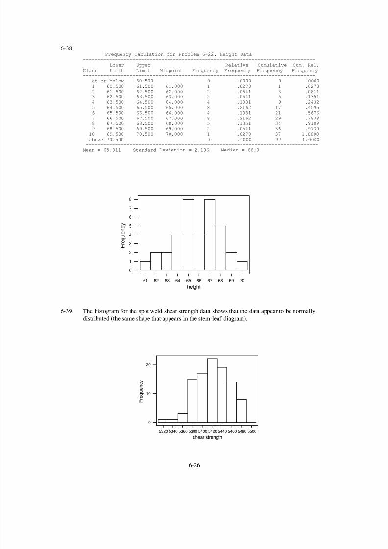
7/12/2019 Solution Manual Stats
http://slidepdf.com/reader/full/solution-manual-stats 159/588
6-38.Frequency Tabulation for Problem 6-22. Height Data
--------------------------------------------------------------------------------
Lower Upper Relative Cumulative Cum. Rel.
Class Limit Limit Midpoint Frequency Frequency Frequency Frequency
--------------------------------------------------------------------------------
at or below 60.500 0 .0000 0 .0000
1 60.500 61.500 61.000 1 .0270 1 .0270
2 61.500 62.500 62.000 2 .0541 3 .0811
3 62.500 63.500 63.000 2 .0541 5 .1351
4 63.500 64.500 64.000 4 .1081 9 .2432
5 64.500 65.500 65.000 8 .2162 17 .4595
6 65.500 66.500 66.000 4 .1081 21 .5676
7 66.500 67.500 67.000 8 .2162 29 .7838
8 67.500 68.500 68.000 5 .1351 34 .9189
9 68.500 69.500 69.000 2 .0541 36 .9730
10 69.500 70.500 70.000 1 .0270 37 1.0000
above 70.500 0 .0000 37 1.0000
--------------------------------------------------------------------------------
Mean = 65.811 Standard Deviation = 2.106 Median = 66.0
61 62 63 64 65 66 67 68 69 70
0
1
2
3
4
5
6
7
8
height
F r e q u e n c y
6-39. The histogram for the spot weld shear strength data shows that the data appear to be normally
distributed (the same shape that appears in the stem-leaf-diagram).
5320 5340 5360 5380 5400 5420 5440 5460 5480 5500
0
10
20
shear strength
F r e q u e n c y
6-26
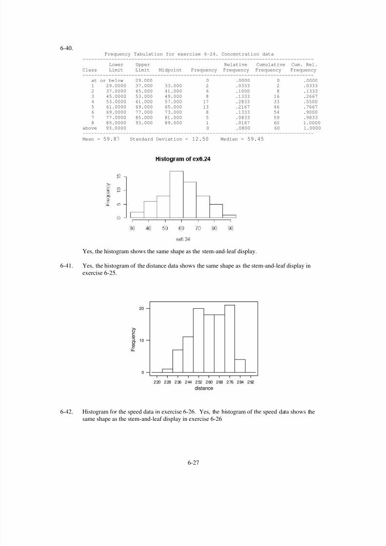
7/12/2019 Solution Manual Stats
http://slidepdf.com/reader/full/solution-manual-stats 160/588
6-40.Frequency Tabulation for exercise 6-24. Concentration data
--------------------------------------------------------------------------------
Lower Upper Relative Cumulative Cum. Rel.
Class Limit Limit Midpoint Frequency Frequency Frequency Frequency
--------------------------------------------------------------------------------
at or below 29.000 0 .0000 0 .0000
1 29.0000 37.000 33.000 2 .0333 2 .0333
2 37.0000 45.000 41.000 6 .1000 8 .1333
3 45.0000 53.000 49.000 8 .1333 16 .2667
4 53.0000 61.000 57.000 17 .2833 33 .5500
5 61.0000 69.000 65.000 13 .2167 46 .7667
6 69.0000 77.000 73.000 8 .1333 54 .9000
7 77.0000 85.000 81.000 5 .0833 59 .9833
8 85.0000 93.000 89.000 1 .0167 60 1.0000
above 93.0000 0 .0800 60 1.0000
--------------------------------------------------------------------------------
Mean = 59.87 Standard Deviation = 12.50 Median = 59.45
Yes, the histogram shows the same shape as the stem-and-leaf display.
6-41. Yes, the histogram of the distance data shows the same shape as the stem-and-leaf display in
exercise 6-25.
220 228 236 244 252 260 268 276 284 292
0
10
20
distance
F r e q u e n c y
6-42. Histogram for the speed data in exercise 6-26. Yes, the histogram of the speed data shows the
same shape as the stem-and-leaf display in exercise 6-26
6-27

7/12/2019 Solution Manual Stats
http://slidepdf.com/reader/full/solution-manual-stats 161/588
620 670 720 770
0
10
20
speed (megahertz)
F r e q u e n c y
6-43. Yes, the histogram of the wine rating data shows the same shape as the stem-and-leaf display in
exercise 6-27.
85 90 95
0
1
2
3
4
5
6
7
rating
F r e q u e n c y
6-28

7/12/2019 Solution Manual Stats
http://slidepdf.com/reader/full/solution-manual-stats 162/588
6-44.
contour
trim
holes/slots
assembly
lubrication
dents
pits
deburr
0
16.2
32.4
48.6
64.8
81
0
20
40
60
80
00
scores
Pareto Chart forAutomobile Defects
percent of total
1
37.0
63.0
72.880.2
86.491.4
96.3100.0
Roughly 63% of defects are described by parts out of contour and parts under trimmed.
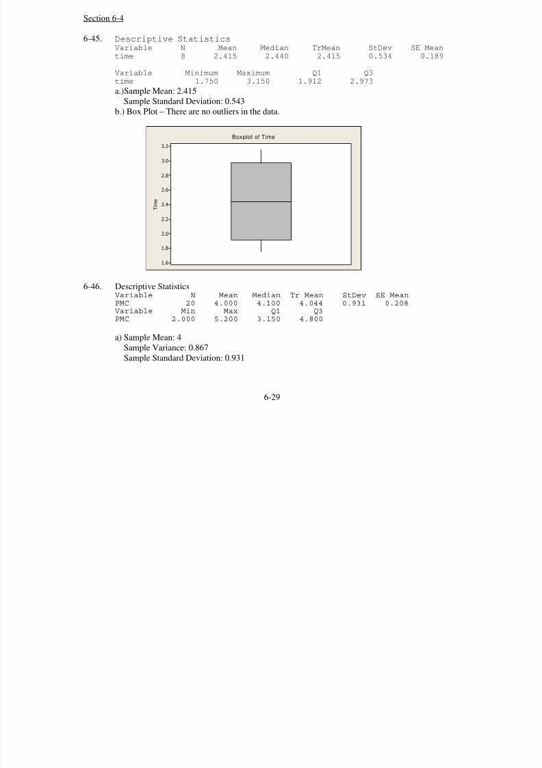
7/12/2019 Solution Manual Stats
http://slidepdf.com/reader/full/solution-manual-stats 163/588
Section 6-4
6-45. Descriptive StatisticsVariable N Mean Median TrMean StDev SE Mean
time 8 2.415 2.440 2.415 0.534 0.189
Variable Minimum Maximum Q1 Q3
time 1.750 3.150 1.912 2.973
a.)Sample Mean: 2.415
Sample Standard Deviation: 0.543
b.) Box Plot – There are no outliers in the data.
T i m e
3.2
3.0
2.8
2.6
2.4
2.2
2.0
1.8
1.6
Boxplot of Time
6-46. Descriptive StatisticsVariable N Mean Median Tr Mean StDev SE MeanPMC 20 4.000 4.100 4.044 0.931 0.208Variable Min Max Q1 Q3PMC 2.000 5.200 3.150 4.800
a) Sample Mean: 4
Sample Variance: 0.867
Sample Standard Deviation: 0.931
6-29

7/12/2019 Solution Manual Stats
http://slidepdf.com/reader/full/solution-manual-stats 164/588
b)
P e r c e n t a g e
5.5
5.0
4.5
4.0
3.5
3.0
2.5
2.0
Boxplot of Percentage
6-47. Descriptive StatisticsVariable N Mean Median Tr Mean StDev SE MeanTemperat 9 952.44 953.00 952.44 3.09 1.03Variable Min Max Q1 Q3
Temperat 948.00 957.00 949.50 955.00
a) Sample Mean: 952.44
Sample Variance: 9.53
Sample Standard Deviation: 3.09
b) Median: 953; Any increase in the largest temperature measurement will not affect the median.c)
T e m p e r a t u
r e
957
956
955
954
953
952
951
950
949
948
Boxplot of Temperatur e
6-48 Descriptive statisticsVariable N Mean Median TrMean StDev SE Mean
drag coefficients 9 83.11 82.00 83.11 7.11 2.37
Variable Minimum Maximum Q1 Q3drag coefficients 74.00 100.00 79.50 84.50
a) Median: 00.82~= x
Upper quartile: Q1 =79.50
Lower Quartile: Q3=84.50
b)
6-30

7/12/2019 Solution Manual Stats
http://slidepdf.com/reader/full/solution-manual-stats 165/588
D r a g C o e f
100
95
90
85
80
75
Boxplot of Drag Coef
c) Variable N Mean Median TrMean StDev SE Mean
drag coefficients 8 81.00 81.50 81.00 3.46 1.22
Variable Minimum Maximum Q1 Q3
drag coefficients 74.00 85.00 79.25 83.75
D r a g C o e f 1
85.0
82.5
80.0
77.5
75.0
Boxplot of Drag Coef1
Removing the largest observation (100) lowers the mean and median. Removing this “outlier
also greatly reduces the variability as seen by the smaller standard deviation and the smaller
difference between the upper and lower quartiles.
6-49. Descriptive Statistics of O-ring joint temperature dataVariable N Mean Median TrMean StDev SE Mean
Temp 36 65.86 67.50 66.66 12.16 2.03
Variable Minimum Maximum Q1 Q3
Temp 31.00 84.00 58.50 75.00
a) Median = 67.50
Lower Quartile: Q1=58.50
Upper Quartile: Q3=75.00
b) Data with lowest point removedVariable N Mean Median TrMean StDev SE Mean
6-31

7/12/2019 Solution Manual Stats
http://slidepdf.com/reader/full/solution-manual-stats 166/588
Temp 35 66.86 68.00 67.35 10.74 1.82
Variable Minimum Maximum Q1 Q3
Temp 40.00 84.00 60.00 75.00
The mean and median have increased and the standard deviation and difference between the upper
and lower quartile has decreased.
c.)Box Plot - The box plot indicates that there is an outlier in the data.
J o i n t T e m p
90
80
70
60
50
40
30
Boxplot of Joint Temp
6-50. This plot conveys the same basic information as the stem and leaf plot but in a different format. The outliers that were
separated from the main portion of the stem and leaf plot are shown here separated from the whiskers.
F u e l
100
95
90
85
Boxplot of Fuel
6-51 The box plot shows the same basic information as the stem and leaf plot but in a different format. The outliers that
were separated from the main portion of the stem and leaf plot are shown here separated from the whiskers.
6-32

7/12/2019 Solution Manual Stats
http://slidepdf.com/reader/full/solution-manual-stats 167/588
B i l l i o n o f k i l o w a t t h o u r s
1800
1600
1400
1200
1000
800
600
400
200
0
Boxplot of Bill ion of kilow att hours
6-52 The box plot and the stem-leaf-diagram show that the data are very symmetrical about the mean. It also
shows that there are no outliers in the data.
C o n c e n t r a t i o n
90
80
70
60
50
40
30
Boxplot of Concentrat ion
6-53.This plot, as the stem and leaf one, indicates that the data fall mostly in one region and that the measurements toward
the ends of the range are more rare.
6-33

7/12/2019 Solution Manual Stats
http://slidepdf.com/reader/full/solution-manual-stats 168/588
W e l d S t r e n g t h
5500
5450
5400
5350
Boxplot of Weld Strength
6-54 The box plot shows that the data are symmetrical about the mean. It also shows that there is an outlier in
the data. These are the same interpretations seen in the stem-leaf-diagram.
S p e e d
775
750
725
700
675
650
Boxplot of Speed
6-55 We can see that the two distributions seem to be centered at different values.
D a t a
MaleFemale
76
74
72
70
68
66
64
62
60
Boxplot of Female, Male
6-56 The box plot shows that there is a difference between the two formulations. Formulation 2 has a
higher mean cold start ignition time and a larger variability in the values of the start times. The
6-34

7/12/2019 Solution Manual Stats
http://slidepdf.com/reader/full/solution-manual-stats 169/588
first formulation has a lower mean cold start ignition time and is more consistent. Care should be
taken, though since these box plots for formula 1 and formula 2 are made using 8 and 10 data
points respectively. More data should be collected on each formulation to get a better
determination.
D a t a
Formula 2Formula 1
3.6
3.2
2.8
2.4
2.0
Boxplot of Formula 1, Formula 2
6.57. All distributions are centered at about the same value, but have different variances.
D a t a
Control_2Control_1ControlHigh Dose
3000
2500
2000
1500
1000
500
0
Boxplot of High Dose, Contr ol, Contr ol_1 , Contr ol_2
6-35

7/12/2019 Solution Manual Stats
http://slidepdf.com/reader/full/solution-manual-stats 170/588
Section 6-5
6-58. Stem-leaf-plot of viscosity N = 40
Leaf Unit = 0.10
2 42 89
12 43 0000112223
16 43 556616 44
16 44
16 45
16 45
16 46
16 46
17 47 2
(4) 47 5999
19 48 000001113334
7 48 5666689
The stem-leaf-plot shows that there are two “different” sets of data. One set of data is centered about 43 and
the second set is centered about 48. The time series plot shows that the data starts out at the higher level and
then drops down to the lower viscosity level at point 24. Each plot gives us a different set of information.
If the specifications on the product viscosity are 48.0±2, then there is a problem with the process
performance after data point 24. An investigation needs to take place to find out why the location of the
process has dropped from around 48.0 to 43.0. The most recent product is not within specification limits.
Index
V i s c o s
i t y
403632282420161284
49
48
47
46
45
44
43
42
Time Series Plot of Viscosity
6-59. Stem-and-leaf display for Force: unit = 1 1|2 represents 12
3 17|558
6 18|357
14 19|00445589
18 20|1399
(5) 21|00238
17 22|005
14 23|5678
10 24|1555899
3 25|158
6-36

7/12/2019 Solution Manual Stats
http://slidepdf.com/reader/full/solution-manual-stats 171/588
Index
P u
l l - o f f F o
r c e
403632282420161284
260
250
240
230
220
210
200
190
180
170
Time Seri es Plot of Pull-off Force
In the time series plot there appears to be a downward trend beginning after time 30. The stem and leaf
plot does not reveal this.
6-60. Stem-and-leaf of Chem Concentration N = 50 Leaf Unit = 0.10
1 16 1
2 16 3
3 16 5
5 16 67
9 16 8899
18 17 000011111
25 17 2233333
25 17 44444444444445555
8 17 6667
4 17 888
1 18 1
Index
C h e m C o n c e n t r a t i o n
50454035302520151051
18.0
17.5
17.0
16.5
16.0
Time Seri es Plot of Chem Concentr ati on
In the time series plot there appears to be fluctuating. The stem and leaf plot does not reveal this.
6-37

7/12/2019 Solution Manual Stats
http://slidepdf.com/reader/full/solution-manual-stats 172/588
6-61. Stem-and-leaf of Wolfer sunspot N = 100 Leaf Unit = 1.0
17 0 01224445677777888
29 1 001234456667
39 2 0113344488
50 3 00145567789
50 4 011234567788
38 5 0457933 6 0223466778
23 7 147
20 8 2356
16 9 024668
10 10 13
8 11 8
7 12 245
4 13 128
1 14
1 15 4
The data appears to decrease between 1790 and 1835, the stem and leaf plot indicates skewed data.
Index
W o l f e r s u n s p o t
1009080706050403020101
160
140
120
100
80
60
40
20
0
Time Seri es Plot of Wol fer sunspot
6-62. Time Series Plot
Index
M i l e s
F l o w n
80726456484032241681
16
14
12
10
8
6
Time Seri es Plot of Miles Flown
6-38

7/12/2019 Solution Manual Stats
http://slidepdf.com/reader/full/solution-manual-stats 173/588
Each year the miles flown peaks during the summer hours. The number of miles flown increased over the
years 1964 to 1970.
Stem-and-leaf of Miles Flown N = 84Leaf Unit = 0.10
1 6 710 7 246678889
22 8 013334677889
33 9 01223466899
(18) 10 022334456667888889
33 11 012345566
24 12 11222345779
13 13 1245678
6 14 0179
2 15 1
1 16 2
When grouped together, the yearly cycles in the data are not seen. The data in the stem-leaf-
diagram appear to be nearly normally distributed.
6-63. Stem-and-leaf of Number of Earthquakes N = 105 Leaf Unit = 1.0
2 0 67
6 0 8888
11 1 00011
19 1 22333333
35 1 4444455555555555
45 1 6666666777
(12) 1 888888889999
48 2 00001111111
37 2 222222223333
25 2 44455
20 2 66667777
12 2 89
10 3 018 3 22
6 3 45
4 3 66
2 3 9
1 4 1
Time Series Plot
Year
N u m b e r o f E a r t h q u a k e s
20902080207020602050204020302020201020001990
45
40
35
30
25
20
15
10
5
Time Series Plot of Number of Eart hquakes
6-39

7/12/2019 Solution Manual Stats
http://slidepdf.com/reader/full/solution-manual-stats 174/588
6-64. Stem-and-leaf of Petroleum Imports N = 32 Leaf Unit = 100
5 5 00149
11 6 012269
15 7 3468
(8) 8 00346889
9 9 4
8 10 1785 11 458
2 12 2
1 13 1
Stem-and-leaf of Total Petroleum Imports as Perc N = 32
Leaf Unit = 10
4 3 2334
9 3 66778
14 4 00124
(7) 4 5566779
11 5 0014
7 5 5688
3 6 013
Stem-and-leaf of Petroleum Imports from Persian N = 32
Leaf Unit = 10
1 0 6
3 0 89
3 1
5 1 33
6 1 4
11 1 66777
16 1 89999
16 2 000011
10 2 2233
6 2 44452 2 67
Time Series plot:
Year
D a
t a
2 0 0 2
1 9 9 9
1 9 9 6
1 9 9 3
1 9 9 0
1 9 8 7
1 9 8 4
1 9 8 1
1 9 7 8
1 9 7 5
14000
12000
10000
8000
6000
4000
2000
0
Variable
Petroleum Imports from Persian
Petroleum Imports
Total Petroleum Imports as Perc
Time Series Plot of Petroleum I m, Total Petrol, Petr oleum Im
6-40

7/12/2019 Solution Manual Stats
http://slidepdf.com/reader/full/solution-manual-stats 175/588
Section 6-6
6-65.
73.99 74.00 74.01 74.02
1
5
10
20
30
40
5060
70
80
90
95
99
Data
P e r c e n t
Normal Probability Plot for 6-1
Piston Ring DiameterML Estimates - 95% CI
Mean
StDev
74.0044
0.0043570
ML Estimates
The pattern of the data indicates that the sample may not come from a normally distributed population or that the
largest observation is an outlier. Note the slight bending downward of the sample data at both ends of the graph.
6-66.
-40 -20 0 20 40 60
1
5
10
20
30
40
5060
70
80
90
95
99
Data
P e r c e n t
Exercise 6-2 Data
Normal Probability Plot for time
Mean
StDev
14.3589
18.3769
ML Estimates
It appears that the data do not come from a normal distribution. Very few of the data points fall on the line.
6-41
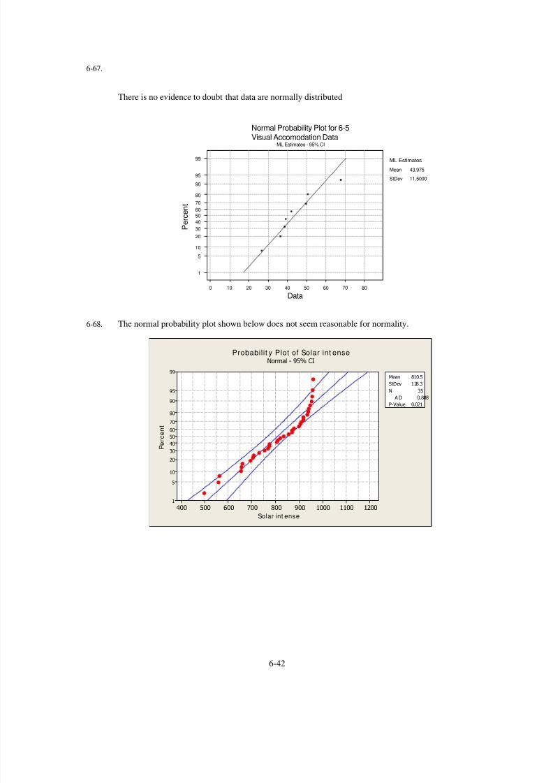
7/12/2019 Solution Manual Stats
http://slidepdf.com/reader/full/solution-manual-stats 176/588
6-67.
There is no evidence to doubt that data are normally distributed
0 10 20 30 40 50 60 70 80
1
5
10
20
30
40
50
60
70
80
90
95
99
Data
P e r c e n t
Normal Probability Plot for 6-5
Visual Accomodation DataML Estimates - 95% CI
Mean
StDev
43.975
11.5000
ML Estimates
6-68. The normal probability plot shown below does not seem reasonable for normality.
Solar int ense
P e r c e n t
120011001000900800700600500400
99
95
90
80
70
60
50
40
30
20
10
5
1
Mean
0.021
810.5
StDev 128.3
N 35
A D 0.888
P-Value
Probabilit y Plot of Solar int enseNormal - 95% CI
6-42

7/12/2019 Solution Manual Stats
http://slidepdf.com/reader/full/solution-manual-stats 177/588
6-69.
30 40 50 60 70 80 90 100
1
5
10
20
30
40
50
60
70
80
90
95
99
Data
P e r c e n t
Normal Probability Plot for temperatureData from exercise 6-13
Mean
StDev
65.8611
11.9888
ML Estimates
The data appear to be normally distributed. Although, there are some departures from the line at the ends
of the distribution.
6-70.
80 90 100
1
5
10
20304050607080
90
95
99
Data
P e r c e n t
Normal Probability Plot for 6-14Octane Rating
ML Estimates - 95% CI
Mean
StDev
90.5256
2.88743
ML Estimates
There are a few points outside the confidence limits, indicating that the sample is not perfectly normal. These
deviations seem to be fairly small though.
6-43

7/12/2019 Solution Manual Stats
http://slidepdf.com/reader/full/solution-manual-stats 178/588
6-71.
0 1000 2000 3000
1
5
10
20304050607080
90
95
99
Data
P e r c e n t
Normal Probability Plot for cycles to failure
Data from exercise 6-15
Mean
StDev
1282.78
539.634
ML Estimates
The data appear to be normally distributed. Although, there are some departures from the line at the ends
of the distribution.
6-72.
9585756555453525
99
95
90
80
7060
50
40
30
20
10
5
1
Data
P e r c e n t
Data from exercise 6-24
Normal Probability Plot for concentration
Mean
StDev
59.8667
12.3932
ML Estimates
The data appear to be normally distributed. Nearly all of the data points fall very close to, or on the line.
6-44

7/12/2019 Solution Manual Stats
http://slidepdf.com/reader/full/solution-manual-stats 179/588
6-73.
Students
Female
Students
Male
75706560
99
95
90
80
70
60
50
40
30
20
10
5
1
Data
P e r c e n t
Normal Probability Plot for 6-22...6-29ML Estimates - 95% CI
Both populations seem to be normally distributed, moreover, the lines seem to be roughly parallel
indicating that the populations may have the same variance and differ only in the value of their mean.
6-74. Yes, it is possible to obtain an estimate of the mean from the 50th percentile value of the normal probability
plot. The fiftieth percentile point is the point at which the sample mean should equal the population mean
and 50% of the data would be above the value and 50% below. An estimate of the standard deviation would
be to subtract the 50th percentile from the 84th percentile These values are based on the values from the z-
table that could be used to estimate the standard deviation.

7/12/2019 Solution Manual Stats
http://slidepdf.com/reader/full/solution-manual-stats 180/588
Supplemental Exercises
6-75. Based on the digidot plot and time series plots of these data, in each year the temperature has a
similar distribution. In each year, the temperature will increase until the mid year and then it starts
to decrease.
6-45

7/12/2019 Solution Manual Stats
http://slidepdf.com/reader/full/solution-manual-stats 181/588
Data
16.215.615.014.413.813.212.6
2000
2001
2002
2003
2004
Dotplot of 2000, 2001, 200 2, 2003, 2004
Index
D a t a
121110987654321
16
15
14
13
12
Variable
2002
2003
2004
2000
2001
Time Series Plot of 200 0, 2001 , 2002, 20 03, 200 4
Stem-and-leaf of C7 N = 60
Leaf Unit = 0.10
3 12 244
15 12 555666677778
23 13 12334444
25 13 55
(7) 14 222223428 14 556
25 15 112222444
16 15 5899
12 16 000000111222
Time-series plot by month over 5 years
6-46

7/12/2019 Solution Manual Stats
http://slidepdf.com/reader/full/solution-manual-stats 182/588
Index
C 7
60544842363024181261
16
15
14
13
12
Time Series Plot of C7
Supplemental Exercises
6-76. a) Sample Mean = 65.083
The sample mean value is close enough to the target value to accept the solution as
conforming. There is a slight difference due to inherent variability.
b) s2
= 1.86869 s = 1.367
c) A major source of variability might be variability in the reagent material. Furthermore, if the
same setup is used for all measurements it is not expected to affect the variability. However, if each measurement uses a different setup, then setup differences could also be a major source of
variability.
A low variance is desirable because it indicates consistency from measurement to measurement. This
implies the measurement error has low variability.
6-77.
The unemployment rate drops steadily from 1997 to 2000 and then increases again quite quickly.
It reaches it’s peak in the middle of 2003 and then begins to drop steadily again.
6-47

7/12/2019 Solution Manual Stats
http://slidepdf.com/reader/full/solution-manual-stats 183/588
Index
C 1 3
117104917865523926131
6.5
6.0
5.5
5.0
4.5
4.0
Time Series Plot of C13
6-78. a) 6001,62433,10
26
1
6
1
2 ==⎟ ⎠
⎞⎜⎝
⎛ = ∑∑
==
n x x
i
i
i
i
Ω=Ω=
Ω=−
−=
−
⎟ ⎠
⎞⎜⎝
⎛
−
=
∑∑ =
=
46.49.19
9.1916
6
001,62433,10
1
2
2
26
16
1
2
2
s
n
n
x
x
s
i
i
i
i
b) 61521353
2
6
1
6
1
2 ==⎟ ⎠ ⎞⎜
⎝ ⎛ = ∑∑
==
n x x
i
i
i
i
6-48

7/12/2019 Solution Manual Stats
http://slidepdf.com/reader/full/solution-manual-stats 184/588
Ω=Ω=
Ω=−
−=
−
⎟ ⎠
⎞⎜⎝
⎛
−
=
∑∑ =
=
46.49.19
9.1916
6
521,1353
1
2
2
26
16
1
2
2
s
n
n
x
x
s
i
i
i
i
Shifting the data from the sample by a constant amount has no effect on the sample variance or standard
deviation.
c) 620010061043300
26
1
6
1
2 ==⎟ ⎠
⎞⎜⎝
⎛ = ∑∑
==
n x x
i
i
i
i
Ω=Ω=
Ω=−
−=
−
⎟ ⎠
⎞⎜⎝
⎛
−
=
∑∑ =
=
61.441990
199016
6
62001001043300
1
2
2
26
16
1
2
2
s
n
n
x
x
s
i
i
i
i
Yes, the rescaling is by a factor of 10. Therefore, s2 and s would be rescaled by multiplying s2 by 102
(resulting in 1990Ω2) and s by 10 (44.6Ω).
6-79 a) Sample 1 Range = 4
Sample 2 Range = 4
Yes, the two appear to exhibit the same variability
b) Sample 1 s = 1.604
Sample 2 s = 1.852
No, sample 2 has a larger standard deviation.
c) The sample range is a relatively crude measure of the sample variability as compared to the sample
standard deviation since the standard deviation uses the information from every data point in the sample
whereas the range uses the information contained in only two data points - the minimum and maximum.
6-80 a.) It appears that the data may shift up and then down over the 80 points.
6-49

7/12/2019 Solution Manual Stats
http://slidepdf.com/reader/full/solution-manual-stats 185/588
10 20 30 40 50 60 70 80
13
14
15
16
17
Index
v i s c o s i t y
b.)It appears that the mean of the second set of 40 data points may be slightly higher than the first set of 40.
c.) Descriptive Statistics: viscosity 1, viscosity 2
Variable N Mean Median TrMean StDev SE Mean
Viscosity1 40 14.875 14.900 14.875 0.948 0.150
Viscosity2 40 14.923 14.850 14.914 1.023 0.162
There is a slight difference in the mean levels and the standard deviations.
6-81.
From the stem-and-leaf diagram, the distribution looks like the uniform distribution. From the
time series plot, there is an increasing trend in energy consumption.
Stem-and-leaf of Energy N = 21
Leaf Unit = 100
4 2 0011
7 2 233
9 2 45
10 2 7
(2) 2 89
9 3 01
7 3 22
5 3 445
2 3 66
6-50

7/12/2019 Solution Manual Stats
http://slidepdf.com/reader/full/solution-manual-stats 186/588
Index
E n e r g y
2018161412108642
3800
3600
3400
3200
3000
2800
2600
2400
2200
2000
Time Series Plot of Energy
6-82
6-76 Second half6-76 First half
17
16
15
14
13
Comparative boxplots for viscosity data
Viscosity
Both sets of data appear to have the same mean although the first half seem to be concentrated a little more tightly.
Two data points appear as outliers in the first half of the data.
6-83
908070605040302010
15
10
5
0
Index
s a l e s
6-51

7/12/2019 Solution Manual Stats
http://slidepdf.com/reader/full/solution-manual-stats 187/588
There appears to be a cyclic variation in the data with the high value of the cycle generally increasing. The
high values are during the winter holiday months.
b) We might draw another cycle, with the peak similar to the last year’s data (1969) at about 12.7 thousand
bottles.
6-84.
Descriptive StatisticsVariable N Mean Median Tr Mean StDev SE Meantemperat 24 48.125 49.000 48.182 2.692 0.549Variable Min Max Q1 Q3temperat 43.000 52.000 46.000 50.000
a) Sample Mean: 48.125
Sample Median: 49
b) Sample Variance: 7.246
Sample Standard Deviation: 2.692
c)
52
51
50
49
48
47
46
45
44
43
t e m p e r a t u r
The data appear to be slightly skewed.
6-85 a)Stem-and-leaf display for Problem 2-35: unit = 1 1|2 represents 12
1 0T|3
8 0F|4444555
18 0S|6666777777
(7) 0o|8888999
15 1*|111
12 1T|22233
7 1F|45
5 1S|77
3 1o|899
b) Sample Average = 9.325
Sample Standard Deviation = 4.4858
6-52

7/12/2019 Solution Manual Stats
http://slidepdf.com/reader/full/solution-manual-stats 188/588
c)
40302010
20
15
10
5
Index
s p r i n g s
The time series plot indicates there was an increase in the average number of nonconforming springs
made during the 40 days. In particular, the increase occurs during the last 10 days.
6-86. a.) Stem-and-leaf of errors N = 20
Leaf Unit = 0.10
3 0 000
10 1 0000000
10 2 0000
6 3 00000
1 4 0
b.) Sample Average = 1.700
Sample Standard Deviation = 1.174
c.)
5 10 15 20
0
1
2
3
4
Index
e r r o r s
The time series plot indicates a slight decrease in the number of errors for strings 16 - 20.
6-53

7/12/2019 Solution Manual Stats
http://slidepdf.com/reader/full/solution-manual-stats 189/588
6-87. The golf course yardage data appear to be skewed. Also, there is an outlying data point above 7500 yards.
6800
6900
7000
7100
7200
7300
7400
7500
y a r d a g e
6-88
half
6-76 First
half
6-76 Second
18171615141312
99
95
90
80
70
60
50
40
30
20
10
5
1
Data
P e r c e n t
Normal Probability Plot for 6-76 First h...6-76 SecondML Estimates - 95% CI
Both sets of data appear to be normally distributed and with roughly the same mean value. The difference in slopes for
the two lines indicates that a change in variance might have occurred. This could have been the result of a change in
processing conditions, the quality of the raw material or some other factor.
6-54

7/12/2019 Solution Manual Stats
http://slidepdf.com/reader/full/solution-manual-stats 190/588
6-89
40 45 50 55
1
5
10
20
30
40
5060
70
80
9095
99
Data
P e r c e n t
Normal Probability Plot for Temperature
Mean
StDev
48.125
2.63490
ML Estimates
There appears to be no evidence that the data are not normally distributed. There are some repeat points in
the data that cause some points to fall off the line.
6-90
6-44
6-56
4.53.52.51.50.5
99
95
90
80
70
60
50
40
30
20
10
5
1
Data
P e r c e n t
Normal Probability Plot for 6-44...6-56ML Estimates - 95% CI
Although we do not have sufficient data points to really see a pattern, there seem to be no significant deviations from
normality for either sample. The large difference in slopes indicates that the variances of the populations are very
different.
6-55

7/12/2019 Solution Manual Stats
http://slidepdf.com/reader/full/solution-manual-stats 191/588
285
275
265
255
245
235
225
D i s t a n c e i n y a r d s
6-91.
The plot indicates that most balls will fall somewhere in the 250-275 range. In general, the population is grouped more
toward the high end of the region. This same type of information could have been obtained from the stem and leaf
graph of problem 6-25.
6-92. a)
-3000 -2000 -1000 0 1000 2000 3000 4000 5000
1
5
10
20
30
40
50
60
70
80
90
95
99
Data
P e r c e n t
Normal Probability Plot for No. of Cycles
Mean
StDev
1051.88
1146.43
ML Estimates
The data do not appear to be normally distributed. There is a curve in the line.
b)
6-56

7/12/2019 Solution Manual Stats
http://slidepdf.com/reader/full/solution-manual-stats 192/588
1 2 3 4
1
5
10
20
30
40
5060
70
80
90
95
99
Data
P e r c e n t
Normal Probability Plot for y*
Mean
StDev
2.75410
0.499916
ML Estimates
After the transformation y*=log(y), the normal probability plot shows no evidence that the data are not normallydistributed.
Trial 1 Trial 2 Trial 3 Trial 4 Trial 5
600
700
800
900
1000
1100
6-93
- There is a difference in the variability of the measurements in the trials. Trial 1 has the most variability
in the measurements. Trial 3 has a small amount of variability in the main group of measurements, but
there are four outliers. Trial 5 appears to have the least variability without any outliers.
- All of the trials except Trial 1 appear to be centered around 850. Trial 1 has a higher mean value
- All five trials appear to have measurements that are greater than the “true” value of 734.5.
- The difference in the measurements in Trial 1 may indicate a “start-up” effect in the data.
There could be some bias in the measurements that is centering the data above the “true” value.
6-57

7/12/2019 Solution Manual Stats
http://slidepdf.com/reader/full/solution-manual-stats 193/588
6-94. a) Descriptive Statistics Variable N N* Mean SE Mean StDev Variance
Density 29 0 5.4197 0.0629 0.3389 0.1148
Variable Minimum Q1 Median Q3 MaximumDensity 4.0700 5.2950 5.4600 5.6150 5.8600
C8
P e r c e n t
6.56.05.55.04.54.0
99
95
90
80
70
60
50
40
30
20
10
5
1
Mean
<0.005
5.420
StDev 0.3389
N 2
AD 1.355
P-Value
Probabili ty Plot of C8Normal - 95% CI
9
b) There does appear to be a low outlier in the data.
c) Due to the very low data point at 4.07, the mean may be lower than it should be. Therefore, the
median would be a better estimate of the density of the earth. The median is not affected by a few
outliers.

7/12/2019 Solution Manual Stats
http://slidepdf.com/reader/full/solution-manual-stats 194/588
Mind Expanding Exercises
8-95 a.) α χ λ χ α α −=<<−
1)2( 2
2,2
2
2,2
1 r r r T P
⎟⎟ ⎠
⎞
⎜⎜⎝
⎛
<<=
−
r r T T P
r r
22
2
2,2
2
2,2
1α α χ
λ
χ
Then a confidence interval for λ
μ 1
= is ⎟⎟
⎠
⎞
⎜⎜
⎝
⎛
−
2
2,2
1
2
2,2
2,
2
r r
r r T T
α α χ χ
b) n = 20 , r = 10 , and the observed value of Tr is 199 + 10(29) = 489.
A 95% confidence interval for λ
1is )98.101,62.28(
59.9
)489(2,
17.34
)489(2=⎟
⎠
⎞⎜⎝
⎛
8-96 dxe
z
dxe
z
x x
2
21
2
2
1
2
11
2
11
−−∫∞−
−=∫∞
=π π
α α
α
Therefore, )(111 α α zΦ=− .
To minimize L we need to minimize subject to)1()1( 21
1 α α −Φ+−Φ −α α α =+ 21
.
Therefore, we need to minimize .)1()1( 11
1 α α α +−Φ+−Φ −
2
2
1
2
2
1
2)1(
2)1(
11
1
1
1
1
α α
α
π α α ∂α ∂
π α ∂α
∂
−
=+−Φ
−=−Φ
−
−
z
z
e
e
Upon setting the sum of the two derivatives equal to zero, we obtain 2
2
12
2
1 α α α z z
ee =−
. This is solved
by . Consequently, andz zα α α1= − 1
α α α α α =−= 111 2,221α α α == .
8.97 a) n=1/2+(1.9/.1)(9.4877/4)
n=46
b) (10-.5)/(9.4877/4)=(1+p)/(1-p)
p=0.6004 between 10.19 and 10.41.
8-98 a)
n
i
n
i
i
allX P
allX P
X P
)2/1()~(
)2/1()~(
2/1)~(
=≥
=≤
=≤
μ
μ
μ
8-39

7/12/2019 Solution Manual Stats
http://slidepdf.com/reader/full/solution-manual-stats 195/588
1
2
1
2
12
2
1
2
1
)()()()(
−
⎟ ⎠
⎞⎜⎝
⎛ =⎟ ⎠
⎞⎜⎝
⎛ =⎟ ⎠
⎞⎜⎝
⎛ +⎟ ⎠
⎞⎜⎝
⎛ =
∩−+=∪nnnn
B AP BP AP B AP
n
ii
X X P B AP
⎟ ⎠
⎞
⎜⎝
⎛ −=<<=∪−2
11))max(~)(min()(1 μ
b) α μ −=<< 1))max(~)(min( ii X X P
The confidence interval is min( X i), max( X i)
8-99 We would expect that 950 of the confidence intervals would include the value of μ. This is due to
9the definition of a confidence interval.
Let X bet the number of intervals that contain the true mean (μ). We can use the large sample
approximation to determine the probability that P(930 < X < 970).
Let 950.01000
950== p 930.0
1000
9301 == p and 970.0
1000
9702 == p
The variance is estimated by1000
)050.0(950.0)1(=
−n
p p
9963.0)90.2()90.2(006892.0
02.0
006892.0
02.0
1000
)050.0(950.0
)950.0930.0(
1000
)050.0(950.0
)950.0970.0()970.0930.0(
=−<−<=⎟ ⎠
⎞⎜⎝
⎛ −<−⎟
⎠
⎞⎜⎝
⎛ <=
⎟⎟⎟⎟
⎠
⎞
⎜⎜⎜⎜
⎝
⎛ −
<−
⎟⎟⎟⎟
⎠
⎞
⎜⎜⎜⎜
⎝
⎛ −
<=<<
Z P Z P Z P Z P
Z P Z P pP
8-40

7/12/2019 Solution Manual Stats
http://slidepdf.com/reader/full/solution-manual-stats 196/588
CHAPTER 8
Section 8-2
8-1 a) The confidence level for n xn x /14.2/14.2 σ μ σ +≤≤− is determined by the
value of z0 which is 2.14. From Table III, Φ(2.14) = P(Z<2.14) = 0.9838 and the
confidence level is 2(0.9838-0.5) = 96.76%.
b) The confidence level for n xn x /49.2/49.2 σ μ σ +≤≤− is determined by the
by the value of z0 which is 2.14. From Table III, Φ(2.49) = P(Z<2.49) = 0.9936 and the
confidence level is is 2(0.9936-0.5) = 98.72%.
c) The confidence level for n xn x /85.1/85.1 σ μ σ +≤≤− is determined by the
by the value of z0 which is 2.14. From Table III, Φ(1.85) = P(Z<1.85) = 0.9678 and the
confidence level is 93.56%.
8-2 a) A zα = 2.33 would give result in a 98% two-sided confidence interval.
b) A zα = 1.29 would give result in a 80% two-sided confidence interval.
c) A zα = 1.15 would give result in a 75% two-sided confidence interval.
8-3 a) A zα = 1.29 would give result in a 90% one-sided confidence interval.
b) A zα = 1.65 would give result in a 95% one-sided confidence interval.
c) A zα = 2.33 would give result in a 99% one-sided confidence interval.
8-4 a) 95% CI for 96.1,100020,10 , ==== z xn σ μ
4.10126.987
)10/20(96.11000)10/20(96.11000
//
≤≤
+≤≤−
+≤≤−
μ
μ
σ μ σ n z xn z x
b) .95% CI for 96.1,100020,25 , ====z xn
σ μ
8.10072.992
)25/20(96.11000)25/20(96.11000
//
≤≤
+≤≤−
+≤≤−
μ
μ
σ μ σ n z xn z x
c) 99% CI for 58.2,100020,10 , ==== z xn σ μ
3.10167.983
)10/20(58.21000)10/20(58.21000
//
≤≤
+≤≤−
+≤≤−
μ
μ
σ μ σ n z xn z x
d) 99% CI for 58.2,100020,25 , ==== z xn σ μ
3.10107.989
)25/20(58.21000)25/20(58.21000
//
≤≤
+≤≤−
+≤≤−
μ
μ
σ μ σ n z xn z x
e) When n is larger, the CI will get narrower. The higher the confidence level, the wider the CI.
8-1

7/12/2019 Solution Manual Stats
http://slidepdf.com/reader/full/solution-manual-stats 197/588
8-5. a) Find n for the length of the 95% CI to be 40. Za/2 = 1.96
84.320
2.39
202.39
20/)20)(96.1(length1/2
2
=⎟ ⎠
⎞⎜⎝
⎛ =
=
==
n
n
n
Therefore, n = 4. b) Find n for the length of the 99% CI to be 40. Za/2 = 2.58
66.620
6.51
206.51
20/)20)(58.2(length1/2
2
=⎟ ⎠
⎞⎜⎝
⎛ =
=
==
n
n
n
Therefore, n = 7.
8-6 Interval (1): 7.32159.3124 ≤≤ μ and Interval (2): 1.32305.3110 ≤≤ μ
Interval (1): half-length =90.8/2=45.4 and Interval (2): half-length =119.6/2=59.8
a) 3.31704.459.31241 =+= x
3.31708.595.31102 =+= x The sample means are the same.
b) Interval (1): 7.32159.3124 ≤≤ μ was calculated with 95% Confidence because it has a
smaller half-length, and therefore a smaller confidence interval. The 99% confidence level will
make the interval larger.
8-7 a) The 99% CI on the mean calcium concentration would be longer.
b) No, that is not the correct interpretation of a confidence interval. The probability that μ is
between 0.49 and 0.82 is either 0 or 1.
c) Yes, this is the correct interpretation of a confidence interval. The upper and lower limits of the
confidence limits are random variables.
8-8 95% Two-sided CI on the breaking strength of yarn: where ⎯ x = 98, σ = 2 , n=9 and z0.025 = 1.96
3.997.96
9/)2(96.1989/)2(96.198
// 025.0025.0
≤≤
+≤≤−
+≤≤−
μ
μ
σ μ σ n z xn z x
8-9 95% Two-sided CI on the true mean yield: where ⎯ x = 90.480, σ = 3 , n=5 and z0.025 = 1.96
11.9385.87
5/)3(96.1480.905/)3(96.1480.90
// 025.0025.0
≤≤
+≤≤−
+≤≤−
μ
μ
σ μ σ n z xn z x
8-10 99% Two-sided CI on the diameter cable harness holes: where ⎯ x =1.5045 , σ = 0.01 , n=10 and
z0.005 = 2.58
5127.14963.1
10/)01.0(58.25045.110/)01.0(58.25045.1
// 005.0005.0
≤≤
+≤≤−
+≤≤−
μ
μ
σ μ σ n z xn z x
8-2

7/12/2019 Solution Manual Stats
http://slidepdf.com/reader/full/solution-manual-stats 198/588
8-11 a) 99% Two-sided CI on the true mean piston ring diameter
For α = 0.01, zα/2 = z0.005 = 2.58 , and ⎯ x = 74.036, σ = 0.001, n=15
x zn
x zn
−⎛
⎝ ⎜
⎞
⎠⎟ ≤ ≤ +
⎛
⎝ ⎜
⎞
⎠⎟0 005 0 005. .
σμ
σ
74 036 2 580 001
15
74 036 2 580001
15
. ..
. ..
−⎛
⎝ ⎜
⎞
⎠⎟ ≤ ≤ +
⎛
⎝ ⎜
⎞
⎠⎟μ
74.0353 ≤ μ ≤ 74.0367
b) 99% One-sided CI on the true mean piston ring diameter
For α = 0.01, zα = z0.01 =2.33 and ⎯ x = 74.036, σ = 0.001, n=15
μ
μ σ
≤⎟⎟ ⎠
⎞⎜⎜⎝
⎛ −
≤−
15
001.033.2036.74
01.0n
z x
74.0354≤ μ
The lower bound of the one sided confidence interval is less than the lower bound of the two-
sided confidence. This is because the Type I probability of 99% one sided confidence interval (or
α = 0.01) in the left tail (or in the lower bound) is greater than Type I probability of 99% two-
sided confidence interval (or α/2 = 0.005) in the left tail.
8-12 a) 95% Two-sided CI on the true mean life of a 75-watt light bulb
For α = 0.05, zα/2 = z0.025 = 1.96 , and ⎯ x = 1014, σ =25 , n=20
⎟⎟ ⎠
⎞⎜⎜⎝
⎛ +≤≤⎟⎟
⎠
⎞⎜⎜⎝
⎛ −
n z x
n z x
σ μ
σ
025.0025.0
10251003
20
2596.11014
20
2596.11014
≤≤
⎟⎟ ⎠
⎞⎜⎜⎝
⎛ +≤≤⎟⎟
⎠
⎞⎜⎜⎝
⎛ −
μ
μ
b) 95% One-sided CI on the true mean piston ring diameter
For α = 0.05, zα = z0.05 =1.65 and ⎯ x = 1014, σ =25 , n=20
μ
μ
μ σ
≤
≤⎟ ⎠
⎞⎜⎝
⎛ −
≤−
1005
20
2565.11014
05.0n
z x
The lower bound of the one sided confidence interval is lower than the lower bound of the two-
sided confidence interval even though the level of significance is the same. This is because all of
the Type I probability (or α) is in the left tail (or in the lower bound).
8-3

7/12/2019 Solution Manual Stats
http://slidepdf.com/reader/full/solution-manual-stats 199/588
8-13 a) 95% two sided CI on the mean compressive strength
zα/2 = z0.025 = 1.96, and ⎯ x = 3250, σ2 = 1000, n=12
x zn
x zn
−⎛
⎝ ⎜
⎞
⎠⎟ ≤ ≤ +
⎛
⎝ ⎜
⎞
⎠⎟0 025 0 025. .
σμ
σ
89.32673232.1112
62.3196.13250
12
62.3196.13250
≤≤
⎟ ⎠
⎞⎜⎝
⎛ +≤≤⎟
⎠
⎞⎜⎝
⎛ −
μ
μ
b) 99% Two-sided CI on the true mean compressive strength
zα/2 = z0.005 = 2.58
⎟ ⎠
⎞⎜⎝
⎛ +≤≤⎟
⎠
⎞⎜⎝
⎛ −
n z x
n z x
σ μ
σ
005.0005.0
6.32733226.412
62.3158.23250
12
62.3158.23250
≤≤
⎟
⎠
⎞⎜
⎝
⎛ +≤≤⎟
⎠
⎞⎜
⎝
⎛ −
μ
μ
The 99% CI is wider than the 95% CI
8-14 95% Confident that the error of estimating the true mean life of a 75-watt light bulb is less than 5
hours.
For α = 0.05, zα/2 = z0.025 = 1.96 , and ⎯σ =25 , E=5
04.965
)25(96.122
2/ =⎟ ⎠
⎞⎜⎝
⎛ =⎟ ⎠
⎞⎜⎝
⎛ =
E
zn
aσ
Always round up to the next number, therefore n = 97
8-15 Set the width to 6 hours with σ = 25, z0.025 = 1.96 solve for n.
78.2663
49
349
3/)25)(96.1(width1/2
2
=⎟ ⎠
⎞⎜⎝
⎛ =
=
==
n
n
n
Therefore, n = 267.
8-16 99% Confident that the error of estimating the true compressive strength is less than 15 psi
For α = 0.01, zα/2 = z0.005 = 2.58 , and ⎯σ =31.62 , E=15
306.2915
)62.31(58.222
2/ ≅=⎟ ⎠
⎞
⎜⎝
⎛ =⎟ ⎠
⎞⎜⎝
⎛ =
E
zn
aσ
Therefore, n=30
8-4

7/12/2019 Solution Manual Stats
http://slidepdf.com/reader/full/solution-manual-stats 200/588
8-17 To decrease the length of the CI by one half, the sample size must be increased by 4 times (22).
ln z 5.0/2/ =σ α
Now, to decrease by half, divide both sides by 2.
4/)2/(
4/)2/(
2/)2/(2/)/(
2
2/
2/
2/
ln z
ln z
ln z
==
=
σ
σ
σ
α
α
α
Therefore, the sample size must be increased by 22.
8-18 If n is doubled in Eq 8-7: ⎟⎟ ⎠
⎞⎜⎜⎝
⎛ +≤≤⎟⎟
⎠
⎞⎜⎜⎝
⎛ −
n z x
n z x
σ μ
σ
α α 2/2/
⎟⎟ ⎠
⎞⎜⎜⎝
⎛ ===
n
z
n
z
n
z
n
z σ σ σ σ α α α α 2/2/2/2/
414.1
1
414.1414.12
The interval is reduced by 0.293 29.3%
If n is increased by a factor of 4 Eq 8-7:
⎟⎟ ⎠
⎞⎜⎜⎝
⎛ ===
n
z
n
z
n
z
n
z σ σ σ σ α α α α 2/2/2/2/
2
1
224
The interval is reduced by 0.5 or ½.
8-19 a) 99% two sided CI on the mean temperature
zα/2 = z0.005 = 2.57, and x = 13.77, σ = 0.5, n=11
⎟⎟ ⎠
⎞⎜⎜⎝
⎛ +≤≤⎟⎟
⎠
⎞⎜⎜⎝
⎛ −
n z x
n z x
σ μ
σ
005.0005.0
157.1413.383
11
5.057.277.13
11
5.057.277.13
≤≤
⎟ ⎠
⎞⎜⎝
⎛ +≤≤⎟
⎠
⎞⎜⎝
⎛ −
μ
μ
b) 95% lower-confidence bound on the mean temperature
For α = 0.05, zα = z0.05 =1.65 and x = 13.77, σ = 0.5, n =11
μ
μ
μ σ
≤
≤⎟⎟ ⎠
⎞⎜⎜⎝
⎛ −
≤−
521.13
11
5.065.177.13
05.0n
z x
c) 95% confidence that the error of estimating the mean temperature for wheat grown is
less than 2 degrees Celsius.
For α = 0.05, zα/2 = z0.025 = 1.96, and σ = 0.5, E = 2
2401.02
)5.0(96.122
2/ =⎟ ⎠
⎞⎜⎝
⎛ =⎟ ⎠
⎞⎜⎝
⎛ =
E
zn
aσ
Always round up to the next number, therefore n = 1.
8-5

7/12/2019 Solution Manual Stats
http://slidepdf.com/reader/full/solution-manual-stats 201/588
d) Set the width to 1.5 degrees Celsius with σ = 0.5, z0.025 = 1.96 solve for n.
707.175.0
98.0
75.098.0
75.0/)5.0)(96.1(width1/2
2
=⎟ ⎠
⎞⎜⎝
⎛ =
=
==
n
n
n
Therefore, n = 2.

7/12/2019 Solution Manual Stats
http://slidepdf.com/reader/full/solution-manual-stats 202/588
Section 8-3
8-20 131.215,025.0 =t 812.110,05.0 =t 325.120,10.0 =t
787.225,005.0 =t 385.330,001.0 =t
8-21 a) b)179.212,025.0 =t 064.224,025.0 =t c) 012.313,005.0 =t
d) 073.415,0005.0 =t
8-22 a) b)761.114,05.0 =t 539.219,01.0 =t c) 467.324,001.0 =t
8-23 95% confidence interval on mean tire life
94.36457.139,6016 === s xn 131.215,025.0 =t
07.6208233.58197
16
94.3645131.27.60139
16
94.3645131.27.60139
15,025.015,025.0
≤≤
⎟⎟ ⎠
⎞⎜⎜⎝
⎛ +≤≤⎟⎟
⎠
⎞⎜⎜⎝
⎛ −
⎟⎟ ⎠
⎞⎜⎜⎝
⎛ +≤≤⎟⎟
⎠
⎞⎜⎜⎝
⎛ −
μ
μ
μ
n
st x
n
st x
8-24 99% lower confidence bound on mean Izod impact strength
25.025.120 === s xn 539.219,01.0 =t
μ
μ
μ
≤
≤⎟⎟ ⎠
⎞⎜⎜⎝
⎛ −
≤⎟⎟ ⎠
⎞⎜⎜⎝
⎛ −
108.1
20
25.0539.225.1
19,01.0n
st x
8-6

7/12/2019 Solution Manual Stats
http://slidepdf.com/reader/full/solution-manual-stats 203/588
8-25 x = 1.10 s = 0.015 n = 25
95% CI on the mean volume of syrup dispensed
For α = 0.05 and n = 25, tα/2,n-1 = t0.025,24 = 2.064
106.11.094
25
015.0064.210.1
25
015.0064.210.1
24,025.024,025.0
≤≤
⎟⎟ ⎠
⎞⎜⎜⎝
⎛ +≤≤⎟⎟
⎠
⎞⎜⎜⎝
⎛ −
⎟⎟
⎠
⎞⎜⎜
⎝
⎛ +≤≤⎟⎟
⎠
⎞⎜⎜
⎝
⎛ −
μ
μ
μ
n
st x
n
st x
8-26 95% confidence interval on mean peak power
163157 === s xn 447.26,025.0 =t
798.329202.300
7315447.2315
716447.2315
6,025.06,025.0
≤≤
⎟⎟ ⎠ ⎞⎜⎜
⎝ ⎛ +≤≤⎟⎟
⎠ ⎞⎜⎜
⎝ ⎛ −
⎟⎟ ⎠
⎞⎜⎜⎝
⎛ +≤≤⎟⎟
⎠
⎞⎜⎜⎝
⎛ −
μ
μ
μ
n
st x
n
st x
8-27 99% upper confidence interval on mean SBP
9.93.11814 === s xn 650.213,01.0 =t
312.125
14
9.9650.23.118
13,005.0
≤
⎟ ⎠
⎞⎜⎝
⎛ +≤
⎟⎟ ⎠
⎞⎜⎜⎝
⎛ +≤
μ
μ
μ
n
st x
8-28 90% CI on the mean frequency of a beam subjected to loads
132.25,n1.53,s231.67, 4,05.1-n/2, ===== t t xα
1.233230.2
5
53.1132.267.231
5
53.1132.267.231
4,05.04,05.0
≤≤
⎟⎟ ⎠
⎞⎜⎜⎝
⎛ −≤≤⎟⎟
⎠
⎞⎜⎜⎝
⎛ −
⎟⎟ ⎠
⎞⎜⎜⎝
⎛ +≤≤⎟⎟
⎠
⎞⎜⎜⎝
⎛ −
μ
μ
μ
n
st x
n
st x
8-7
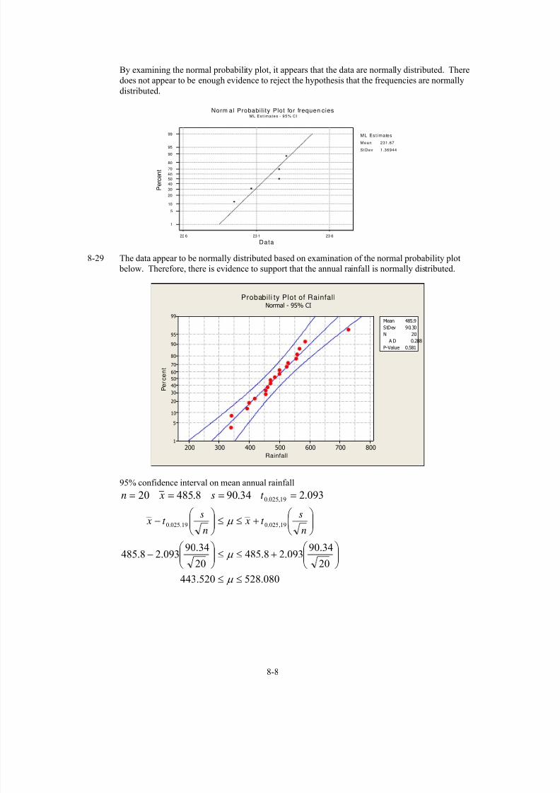
7/12/2019 Solution Manual Stats
http://slidepdf.com/reader/full/solution-manual-stats 204/588
By examining the normal probability plot, it appears that the data are normally distributed. There
does not appear to be enough evidence to reject the hypothesis that the frequencies are normally
distributed.
23 623 122 6
99
95
90
80
70
60
50
40
30
20
10
5
1
Data
P e r c e n t
Norm al Probabil ity Plot for frequen ciesML Est ima tes - 95% CI
Mean
StDev
231.67
1.36944
ML Est imates
8-29 The data appear to be normally distributed based on examination of the normal probability plot
below. Therefore, there is evidence to support that the annual rainfall is normally distributed.
Rainfall
P e r c e n t
800700600500400300200
99
95
90
80
70
60
50
40
30
20
10
5
1
Mean
0.581
485.9
StDev 90.30
N 20
A D 0.288
P-Value
Probabili ty Plot of RainfallNormal - 95% CI
95% confidence interval on mean annual rainfall
34.908.48520 === s xn 093.219,025.0 =t
080.528520.443
20
34.90093.28.48520
34.90093.28.485
19,025.019,025.0
≤≤
⎟⎟ ⎠ ⎞⎜⎜
⎝ ⎛ +≤≤⎟⎟
⎠ ⎞⎜⎜
⎝ ⎛ −
⎟⎟ ⎠
⎞⎜⎜⎝
⎛ +≤≤⎟⎟
⎠
⎞⎜⎜⎝
⎛ −
μ
μ
μ
n
st x
n
st x
8-8

7/12/2019 Solution Manual Stats
http://slidepdf.com/reader/full/solution-manual-stats 205/588
8-30 The data appear to be normally distributed based on examination of the normal probability plot
below. Therefore, there is evidence to support that the solar energy is normally distributed.
Solar
P e r c e n t
80757065605550
99
95
90
80
70
60
50
40
30
20
10
5
1
Mean
0.349
65.58
StDev 4.225
N 16
A D 0.386
P-Value
Probabili ty Plot of SolarNormal - 95% CI
95% confidence interval on mean solar energy consumed
225.458.6516 === s xn 131.215,025.0 =t
831.67329.63
16
225.4131.258.65
16
225.4131.258.65
15,025.015,025.0
≤≤
⎟⎟ ⎠
⎞⎜⎜⎝
⎛ +≤≤⎟⎟
⎠
⎞⎜⎜⎝
⎛ −
⎟⎟ ⎠
⎞⎜⎜⎝
⎛ +≤≤⎟⎟
⎠
⎞⎜⎜⎝
⎛ −
μ
μ
μ
n
st x
n
st x
8-31 99% confidence interval on mean current required
Assume that the data are a random sample from a normal distribution.
7.152.31710 === s xn 250.39,005.0 =t
34.33306.301
10
7.15250.32.317
10
7.15250.32.317
9,005.09,005.0
≤≤
⎟⎟ ⎠
⎞⎜⎜⎝
⎛ +≤≤⎟⎟
⎠
⎞⎜⎜⎝
⎛ −
⎟⎟ ⎠
⎞⎜⎜⎝
⎛ +≤≤⎟⎟
⎠
⎞⎜⎜⎝
⎛ −
μ
μ
μ
n
st x
n
st x
8-9

7/12/2019 Solution Manual Stats
http://slidepdf.com/reader/full/solution-manual-stats 206/588
8-32 a) The data appear to be normally distributed based on examination of the normal probability plot
below. Therefore, there is evidence to support that the level of polyunsaturated fatty acid is normally
distributed.
16 17 18
1
5
10
20
30
40
5060
70
80
90
95
99
Data
P e r c e n t
Normal Probability Plot for 8-25ML Estimates - 95% CI
b) 99% CI on the mean level of polyunsaturated fatty acid.
For α = 0.01, tα/2,n-1 = t0.005,5 = 4.032
⎟⎟ ⎠
⎞⎜⎜⎝
⎛ +≤≤⎟⎟
⎠
⎞⎜⎜⎝
⎛ −
n
st x
n
st x 5,005.05,005.0 μ
505.17455.16
6
319.0032.498.16
6
319.0032.498.16
≤≤
⎟⎟ ⎠
⎞⎜⎜⎝
⎛ +≤≤⎟⎟
⎠
⎞⎜⎜⎝
⎛ −
μ
μ
The 99% confidence for the mean polyunsaturated fat is (16.455, 17.505). There is high
confidence that the true mean is in this interval
8-33 a) The data appear to be normally distributed based on examination of the normal probability
plot below.
235022502150
99
95
90
80
70
60
50
40
30
20
10
5
1
Data
P e r c e n t
Normal Probability Plot for StrengthML Estimates - 95% CI
Mean
StDev
2259.92
34.0550
ML Estimates
8-10

7/12/2019 Solution Manual Stats
http://slidepdf.com/reader/full/solution-manual-stats 207/588
b) 95% two-sided confidence interval on mean comprehensive strength
35.62259.912 === s xn 201.211,025.0 =t
5.22823.2237
126.35201.29.2259
126.35201.29.2259
11,025.011,025.0
≤≤
⎟ ⎠ ⎞⎜
⎝ ⎛ +≤≤⎟
⎠ ⎞⎜
⎝ ⎛ −
⎟⎟ ⎠
⎞⎜⎜⎝
⎛ +≤≤⎟⎟
⎠
⎞⎜⎜⎝
⎛ −
μ
μ
μ
n
st x
n
st x
c) 95% lower-confidence bound on mean strength
μ
μ
μ
≤
≤⎟ ⎠
⎞⎜⎝
⎛ −
≤⎟⎟ ⎠
⎞⎜⎜⎝
⎛ −
4.2241
12
6.35796.19.2259
11,05.0n
st x
8-34 a) According to the normal probability plot there does not seem to be a severe deviation from
normality for this data. This is due to the fact that the data appears to fall along a straight line.
8.308.258.208.15
99
95
90
8070
6050
40
30
20
10
5
1
Data
P e r c e n t
Norm al Probab ility Plot for 8-27ML Est imates - 95% C I
b) 95% two-sided confidence interval on mean rod diameter
For α = 0.05 and n = 15, tα/2,n-1 = t0.025,14 = 2.145
⎟⎟ ⎠
⎞⎜⎜⎝
⎛ +≤≤⎟⎟
⎠
⎞⎜⎜⎝
⎛ −
n
st x
n
st x 14,025.014,025.0 μ
⎟ ⎠
⎞⎜⎝
⎛ +≤≤⎟
⎠
⎞⎜⎝
⎛ −
15
025.0145.223.8
15
025.0145.223.8 μ
8.216 ≤ μ ≤ 8.244
8-11

7/12/2019 Solution Manual Stats
http://slidepdf.com/reader/full/solution-manual-stats 208/588
c) 95% upper confidence bound on mean rod diameter t0.05,14 = 1.761
241.815
025.0761.123.8
14,025.0
≤
⎟⎟
⎠
⎞⎜⎜
⎝
⎛ +≤
⎟⎟ ⎠
⎞⎜⎜⎝
⎛ +≤
μ
μ
μ
n
st x
8-35 a) The data appear to be normally distributed based on examination of the normal probability plot
below. Therefore, there is evidence to support that the speed-up of CNN is normally distributed.
Speed
P e r c e n t
6.05.55.04.54.03.53.0
99
95
90
80
70
60
50
40
30
20
10
5
1
Mean
0.745
4.313
StDev 0.4328
N 1
A D 0.233
P-Value
Probabilit y Plot of SpeedNormal - 95% CI
3
b) 95% confidence interval on mean speed-up
4328.0313.413 === s xn 179.212,025.0 =t
575.4051.4
13
4328.0179.2313.4
13
4328.0179.2313.4
12,025.012,025.0
≤≤
⎟⎟ ⎠
⎞⎜⎜⎝
⎛ +≤≤⎟⎟
⎠
⎞⎜⎜⎝
⎛ −
⎟⎟ ⎠ ⎞
⎜⎜⎝ ⎛ +≤≤⎟⎟
⎠ ⎞
⎜⎜⎝ ⎛ −
μ
μ
μ
n
st x
n
st x
c) 95% lower confidence bound on mean speed-up
4328.0313.413 === s xn 782.112,05.0 =t
μ
μ
μ
≤
≤⎟⎟ ⎠
⎞⎜⎜⎝
⎛ −
≤⎟⎟ ⎠
⎞
⎜⎜⎝
⎛ −
099.4
13
4328.0782.1313.4
12,05.0 n
st x
8-12

7/12/2019 Solution Manual Stats
http://slidepdf.com/reader/full/solution-manual-stats 209/588
8-36 95% lower bound confidence for the mean wall thickness
given x = 4.05 s = 0.08 n = 25
tα,n-1 = t0.05,24 = 1.711
μ ≤⎟⎟
⎠
⎞⎜⎜
⎝
⎛ −
n
st x 24,05.0
μ ≤⎟⎟ ⎠
⎞⎜⎜⎝
⎛ −
25
08.0711.105.4
4.023 ≤ μ
There is high confidence that the true mean wall thickness is greater than 4.023 mm.
3.23.13.02.92.82.72.6
99
95
90
80
70
60
50
40
30
20
10
5
1
Data
P e r c e n t
Normal Probability Plot for Percent EnrichmentML Estimates - 95% CI
Mean
StDev
2.90167
0.0951169
ML Estimates
8-37 a) The data appear to be normally distributed. There is not strong evidence that the percentage of
enrichment deviates from normality.
b) 99% two-sided confidence interval on mean percentage enrichment
For α = 0.01 and n = 12, tα/2,n-1 = t0.005,11 = 3.106, 0.0993s2.9017 == x
991.2813.2
12
0.0993106.3902.2
12
0.0993106.3902.2
11,005.011,005.0
≤≤
⎟ ⎠
⎞⎜⎝
⎛ +≤≤⎟
⎠
⎞⎜⎝
⎛ −
⎟⎟ ⎠
⎞⎜⎜⎝
⎛ +≤≤⎟⎟
⎠
⎞⎜⎜⎝
⎛ −
μ
μ
μ
n
st x
n
st x
8-13
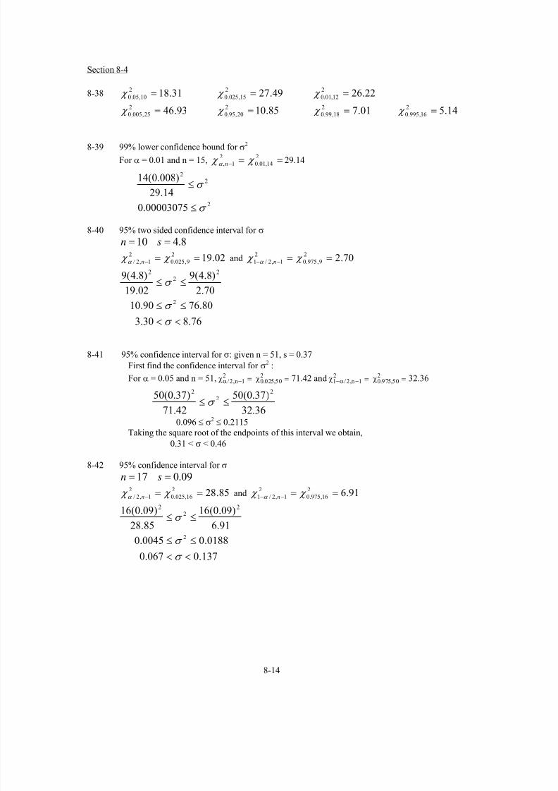
7/12/2019 Solution Manual Stats
http://slidepdf.com/reader/full/solution-manual-stats 210/588
Section 8-4
8-38 31.182
10,05.0 = χ 49.272
15,025.0 = χ 22.262
12,01.0 = χ
93.462
25,005.0 = χ 85.102
20,95.0 = χ 01.72
18,99.0 = χ 14.52
16,995.0 = χ
8-39 99% lower confidence bound for σ2
For α = 0.01 and n = 15, 29.14=−
2
1,nα χ =
2
14,01.0 χ
2
22
00003075.0
14.29
)008.0(14
σ
σ
≤
≤
8-40 95% two sided confidence interval for σ
8.410 == sn
02.192
9,025.0
2
1,2/ ==−
χ χ α n
and 70.22
9,975.0
2
1,2/1 ==−−
χ χ α n
76.830.3
80.7690.10
70.2
)8.4(9
02.19
)8.4(9
2
22
2
<<
≤≤
≤≤
σ
σ
σ
8-41 95% confidence interval for σ: given n = 51, s = 0.37
First find the confidence interval for σ2 :
For α = 0.05 and n = 51, 71.42 and 32.36χα / ,2 12
n− = χ0 025 502. , = χ α1 2 1
2− − =/ ,n χ0 975 50
2. , =
36.32
)37.0(50
42.71
)37.0(50 22
2
≤≤ σ
0.096 ≤ σ2 ≤ 0.2115
Taking the square root of the endpoints of this interval we obtain,
0.31 < σ < 0.46
8-42 95% confidence interval for σ
09.017 == sn
85.282
16,025.0
2
1,2/ ==−
χ χ α n
and 91.62
16,975.0
2
1,2/1 ==−−
χ χ α n
137.0067.00188.00045.0
91.6
)09.0(16
85.28
)09.0(16
2
22
2
<<≤≤
≤≤
σ
σ
σ
8-14

7/12/2019 Solution Manual Stats
http://slidepdf.com/reader/full/solution-manual-stats 211/588
8-43 The data appear to be normally distributed based on examination of the normal probability plot
below. Therefore, there is evidence to support that the mean temperature is normally distributed.
Mean Temp
P e r c e n t
252423222120191817
99
95
90
80
70
60
50
40
30
20
10
5
1
Mean
0.367
21.41StDev 0.9463
N 8
AD 0.352
P-Value
Probabil it y Plot of Mean TempNormal - 95% CI
95% confidence interval for σ
9463.08 == sn
01.162
7,025.0
2
1,2/ ==−
χ χ α n
and 69.12
7,975.0
2
1,2/1 ==−−
χ χ α n
926.1626.0
709.3392.0
69.1
)9463.0(7
01.16
)9463.0(7
2
22
2
<<
≤≤
≤≤
σ
σ
σ
8-44 95% confidence interval for σ
99.1541 == sn
34.592
40,025.0
2
1,2/ ==−
χ χ α n
and 43.242
40,975.0
2
1,2/1 ==−−
χ χ α n
46.2013.13
633.41835.172
43.24
)99.15(40
34.59
)99.15(40
2
22
2
<<
≤≤
≤≤
σ
σ
σ
The data don’t appear to be normally distributed based on examination of the normal probability plot
below. Therefore, there is not enough evidence to support that the time of tumor appearance is normallydistributed. So the 95% confidence interval for σ is invalid.
8-15
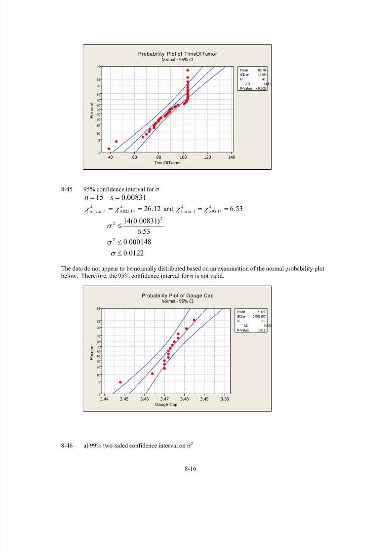
7/12/2019 Solution Manual Stats
http://slidepdf.com/reader/full/solution-manual-stats 212/588
TimeOfTumor
P e r c e n t
140120100806040
99
95
90
80
70
60
50
40
30
20
10
5
1
Mean
<0.005
88.78
S tDev 15.99
N 4
AD 1.631
P-Value
Probability Plot of TimeOfTumorNormal - 95% CI
1
8-45 95% confidence interval for σ 00831.015 == sn
12.262
14,025.0
2
1,2/ ==−
χ χ α n
and 53.62
14,95.0
2
1,1 ==−−
χ χ α n
0122.0
000148.0
53.6
)00831.0(14
2
22
≤
≤
≤
σ
σ
σ
The data do not appear to be normally distributed based on an examination of the normal probability plot
below. Therefore, the 95% confidence interval for σ is not valid.
Gauge Cap
P e r c e n t
3.503.493.483.473.463.453.44
99
95
90
80
70
60
50
40
30
20
10
5
1
Mean
0.018
3.472
StDev 0.008307
N 1
AD 0.878
P-Value
Probability Plot of Gauge CapNormal - 95% CI
5
8-46 a) 99% two-sided confidence interval on σ2
8-16

7/12/2019 Solution Manual Stats
http://slidepdf.com/reader/full/solution-manual-stats 213/588
and913.110 == sn 59.232
9,005.0 = χ 73.12
9,995.0 = χ
038.19396.1
73.1
)913.1(9
59.23
)913.1(9
2
22
2
≤≤
≤≤
σ
σ
b) 99% lower confidence bound for σ2
For α = 0.01 and n = 10, 21.67=−
2
1,nα χ =
2
9,01.0 χ
2
22
5199.1
67.21
)913.1(9
σ
σ
≤
≤
c) 90% lower confidence bound for σ2
For α = 0.1 and n = 10, 14.68=−
2
1,nα χ =
2
9,1.0 χ
σ
σ
σ
≤
≤
≤
498.1
2436.268.14
)913.1(9
2
22
d) The lower confidence bound of the 99% two-sided interval is less than the one-sided interval.
The lower confidence bound for σ2 is in part (c) is greater because the confidence is lower.

7/12/2019 Solution Manual Stats
http://slidepdf.com/reader/full/solution-manual-stats 214/588
Section 8-5
8-47 a) 95% Confidence Interval on the fraction defective produced with this tool.
04333.0300
13ˆ == p 300=n 96.12/ =
α z
06637.002029.0
300
)95667.0(04333.096.104333.0
300
)95667.0(04333.096.104333.0
)ˆ1(ˆˆ
)ˆ1(ˆˆ
2/2/
≤≤
+≤≤−
−+≤≤
−−
p
p
n
p p z p p
n
p p z p
α α
b) 95% upper confidence bound 65.105.0 == z zα
06273.0
300
)95667.0(04333.0650.104333.0
)ˆ1(ˆˆ
2/
≤
+≤
−+≤
p
p
n
p p z p p
α
8-17

7/12/2019 Solution Manual Stats
http://slidepdf.com/reader/full/solution-manual-stats 215/588
8-48 a) 95% Confidence Interval on the proportion of such tears that will heal.
676.0ˆ = p 37=n 96.12/ =α
z
827.05245.0
37
)324.0(676.096.1676.0
37
)324.0(676.096.1676.0
)ˆ1(ˆˆ
)ˆ1(ˆˆ
2/2/
≤≤
+≤≤−
−+≤≤
−−
p
p
n
p p z p p
n
p p z p
α α
b) 95% lower confidence bound on the proportion of such tears that will heal.
p
p
pn
p p z p
≤
≤−
≤−
−
549.0
37
)33.0(676.064.1676.0
)ˆ1(ˆˆ
α
8-49 a) 95% confidence interval for the proportion of college graduates in Ohio that voted for
George Bush.
536.0768
412ˆ == p 768=n 96.12/ =
α z
571.0501.0768
)464.0(536.096.1536.0
768
)464.0(536.096.1536.0
)ˆ1(ˆˆ
)ˆ1(ˆˆ
2/2/
≤≤
+≤≤−
−+≤≤
−−
p
p
n
p p z p p
n
p p z p
α α
b) 95% lower confidence bound on the proportion of college graduates in Ohio that voted for
George Bush.
p
p
pn
p p z p
≤
≤−
≤−
−
506.0
768
)464.0(536.064.1536.0
)ˆ1(ˆˆ
α
8-50 a) 95% Confidence Interval on the death rate from lung cancer.
823.01000
823ˆ == p 1000=n 96.12/ =
α z
8-18

7/12/2019 Solution Manual Stats
http://slidepdf.com/reader/full/solution-manual-stats 216/588
8467.07993.0
1000
)177.0(823.096.1823.0
1000
)177.0(823.096.1823.0
)ˆ1(ˆˆ
)ˆ1(ˆˆ
2/2/
≤≤
+≤≤−
−+≤≤
−−
p
p
n
p p z p p
n
p p z p
α α
b) E = 0.03, α = 0.05, zα/2 = z0.025 = 1.96 and p = 0.823 as the initial estimate of p,
79.621)823.01(823.003.0
96.1)ˆ1(ˆ
22
2/ =−⎟ ⎠
⎞⎜⎝
⎛ =−⎟ ⎠
⎞⎜⎝
⎛ = p p
E
zn α
,
n ≅ 622.
c) E = 0.03, α = 0.05, zα/2 = z0.025 = 1.96 at least 95% confident
11.1067)25.0(03.0
96.1)25.0(
22
2/ =⎟ ⎠
⎞⎜⎝
⎛ =⎟ ⎠
⎞⎜⎝
⎛ =
E
zn α
,
n ≅ 1068.
8-51 a) 95% Confidence Interval on the proportion of rats that are under-weight.
4.030
12ˆ == p 30=n 96.12/ =
α z
575.0225.0
30
)6.0(4.096.14.0
30
)6.0(4.096.14.0
)ˆ1(ˆˆ
)ˆ1(ˆˆ
2/2/
≤≤
+≤≤−
−+≤≤
−−
p
p
n
p p z p p
n
p p z p
α α
b) E = 0.02, α = 0.05, zα/2 = z0.025 = 1.96 and p = 0.4as the initial estimate of p,
96.2304)4.01(4.002.0
96.1)ˆ1(ˆ
22
2/ =−⎟ ⎠
⎞⎜⎝
⎛ =−⎟ ⎠
⎞⎜⎝
⎛ = p p
E
zn α
,
n ≅ 2305.
c) E = 0.02, α = 0.05, zα/2 = z0.025 = 1.96 at least 95% confident
2401)25.0(02.0
96.1)25.0(
22
2/ =⎟ ⎠
⎞⎜⎝
⎛ =⎟ ⎠
⎞⎜⎝
⎛ =
E
zn α
.
8-52 a) 95% Confidence Interval on the true proportion of helmets showing damage
36.050
18ˆ == p 50=n 96.12/ =
α z
8-19

7/12/2019 Solution Manual Stats
http://slidepdf.com/reader/full/solution-manual-stats 217/588
493.0227.0
50
)64.0(36.096.136.0
50
)64.0(36.096.136.0
)ˆ1(ˆˆ
)ˆ1(ˆˆ
2/2/
≤≤
+≤≤−
−+≤≤
−−
p
p
n
p p z p p
n
p p z p
α α
b) 76.2212)36.01(36.002.0
96.1)1(
22
2/ =−⎟ ⎠
⎞⎜⎝
⎛ =−⎟ ⎠
⎞⎜⎝
⎛ = p p
E
zn α
2213≅n
c) 2401)5.01(5.002.0
96.1)1(
22
2/ =−⎟ ⎠
⎞⎜⎝
⎛ =−⎟ ⎠
⎞⎜⎝
⎛ = p p
E
zn α
8-53 The worst case would be for p = 0.5, thus with E = 0.05 and α = 0.01, zα/2 = z0.005 = 2.58 we
obtain a sample size of:
64.665)5.01(5.005.0
58.2)1(
22
2/ =−⎟ ⎠
⎞⎜⎝
⎛ =−⎟ ⎠
⎞⎜⎝
⎛ = p p E
zn α
, n ≅ 666
8-54 E = 0.017, α = 0.01, zα/2 = z0.005 = 2.58
13.5758)5.01(5.0017.0
58.2)1(
22
2/ =−⎟ ⎠
⎞⎜⎝
⎛ =−⎟ ⎠
⎞⎜⎝
⎛ = p p E
zn α
, n ≅ 5759

7/12/2019 Solution Manual Stats
http://slidepdf.com/reader/full/solution-manual-stats 218/588
Section 8-7
8-55 95% prediction interval on the life of the next tire
given x = 60139.7 s = 3645.94 n = 16
for α=0.05 tα/2,n-1 = t0.025,15 = 2.131
3.681481.52131
16
11)94.3645(131.27.60139
16
11)94.3645(131.27.60139
11
11
1
1
15,025.0115,025.0
≤≤
++≤≤+−
++≤≤+−
+
+
+
n
n
n
x
x
nst x x
nst x
The prediction interval is considerably wider than the 95% confidence interval (58,197.3 ≤ μ ≤
62,082.07). This is expected because the prediction interval needs to include the variability in the
parameter estimates as well as the variability in a future observation.
8-56 99% prediction interval on the Izod impact data
8-20

7/12/2019 Solution Manual Stats
http://slidepdf.com/reader/full/solution-manual-stats 219/588
25.025.120 === s xn 861.219,005.0 =t
983.1517.0
2011)25.0(861.225.1
2011)25.0(861.225.1
11
11
1
1
19,005.0119,005.0
≤≤
++≤≤+−
++≤≤+−
+
+
+
n
n
n
x
x
nst x x
nst x
The lower bound of the 99% prediction interval is considerably lower than the 99% confidence
interval (1.108 ≤ μ ≤ ∞). This is expected because the prediction interval needs to include the
variability in the parameter estimates as well as the variability in a future observation.
8-57 95% Prediction Interval on the volume of syrup of the next beverage dispensed
x = 1.10 s = 0.015 n = 25 tα/2,n-1 = t0.025,24 = 2.064
13.1068.1
25
11)015.0(064.210.1
25
11)015.0(064.210.1
11
11
1
1
24,025.0124,025.0
≤≤
+−≤≤+−
++≤≤+−
+
+
+
n
n
n
x
x
nst x xnst x
The prediction interval is wider than the confidence interval: 106.11.094 ≤≤ μ
8-58 90% prediction interval the value of the natural frequency of the next beam of this type that will
be tested. given⎯ x = 231.67, s =1.53 For α = 0.10 and n = 5, tα/2,n-1 = t0.05,4 = 2.132
2.2351.228
5
11)53.1(132.267.231
5
11)53.1(132.267.231
11
11
1
1
4,05.014,05.0
≤≤
+−≤≤+−
++≤≤+−
+
+
+
n
n
n
x
x
nst x xnst x
The 90% prediction in interval is greater than the 90% CI.
8-59 95% Prediction Interval on the volume of syrup of the next beverage dispensed
34.908.48520 === s xn tα/2,n-1 = t0.025,19 = 2.093
551.679049.292
20
11)34.90(093.28.485
20
11)34.90(093.28.485
1111
1
1
19,025.0119,025.0
≤≤
+−≤≤+−
++≤≤+−
+
+
+
n
n
n
x
x
nst x x
nst x
The 95% prediction interval is wider than the 95% confidence interval.
8-60 99% prediction interval on the polyunsaturated fat
8-21

7/12/2019 Solution Manual Stats
http://slidepdf.com/reader/full/solution-manual-stats 220/588
319.098.166 === s xn 032.45,005.0 =t
37.1859.15
611)319.0(032.498.16
611)319.0(032.498.16
11
11
1
1
5,005.015,005.0
≤≤
++≤≤+−
++≤≤+−
+
+
+
n
n
n
x
x
nst x x
nst x
The length of the prediction interval is much longer than the width of the confidence interval
505.17455.16 ≤≤ μ .
8-61 Given x = 317.2 s = 15.7 n = 10 for α=0.05 tα/2,n-1 = t0.005,9 = 3.250
7.3707.263
10
11)7.15(250.32.317
10
11)7.15(250.32.317
11
11
1
1
9,005.019,005.0
≤≤
+−≤≤+−
++≤≤+−
+
+
+
n
n
n
x
x
nst x x
nst x
The length of the prediction interval is longer.
8-62 95% prediction interval on the next rod diameter tested
025.023.815 === s xn 145.214,025.0 =t
29.817.8
15
11)025.0(145.223.8
15
11)025.0(145.223.8
11
11
1
1
14,025.0114,025.0
≤≤
+−≤≤+−
++≤≤+−
+
+
+
n
n
n
x
x
nst x x
nst x
95% two-sided confidence interval on mean rod diameter is 8.216 ≤ μ ≤ 8.244
8-63 90% prediction interval on the next specimen of concrete tested
given x = 2260 s = 35.57 n = 12 for α = 0.05 and n = 12, tα/2,n-1 = t0.05,11 = 1.796
5.23265.2193
12
11)57.35(796.12260
12
11)57.35(796.12260
11
11
1
1
11,05.0111,05.0
≤≤
++≤≤+−
++≤≤+−
+
+
+
n
n
n
x
x
nst x x
nst x
8-64 90% prediction interval on wall thickness on the next bottle tested.
8-22

7/12/2019 Solution Manual Stats
http://slidepdf.com/reader/full/solution-manual-stats 221/588
given x = 4.05 s = 0.08 n = 25 for tα/2,n-1 = t0.05,24 = 1.711
19.491.325
11)08.0(711.105.4
25
11)08.0(711.105.4
11
11
1
1
24,05.0124,05.0
≤≤
+−≤≤+−
++≤≤+−
+
+
+
n
n
n
x
x
nst x x
nst x
8-65 90% prediction interval for enrichment data given x= 2.9 s = 0.099 n = 12 for α = 0.10
and n = 12, tα/2,n-1 = t0.05,11 = 1.796
09.371.2
12
11)099.0(796.19.2
12
11)099.0(796.19.2
11
11
1
1
12,05.0112,05.0
≤≤
++≤≤+−
++≤≤+−
+
+
+
n
n
n
x
x
nst x x
nst x
The 90% confidence interval is
95.285.2
12
1)099.0(796.19.2
12
1)099.0(796.19.2
1112,05.012,05.0
≤≤
−≤≤−
+≤≤−
μ
μ
μ n
st xn
st x
The prediction interval is wider than the CI on the population mean with the same confidence.
The 99% confidence interval is
99.281.2
12
1)099.0(106.39.2
12
1)099.0(106.39.2
1112,005.012,005.0
≤≤
+≤≤−
+≤≤−
μ
μ
μ n
st xn
st x
The prediction interval is even wider than the CI on the population mean with greater confidence.
8-66 To obtain a one sided prediction interval, use t α,n-1 instead of tα/2,n-1
Since we want a 95% one sided prediction interval, tα/2,n-1 = t0.05,24 = 1.711
and x = 4.05 s = 0.08 n = 25
1
1
124,05.0
91.3
25
11)08.0(711.105.4
11
+
+
+
≤
≤+−
≤+−
n
n
n
x
x
xn
st x
The prediction interval bound is much lower than the confidence interval bound of
8-23

7/12/2019 Solution Manual Stats
http://slidepdf.com/reader/full/solution-manual-stats 222/588
4.023 mm

7/12/2019 Solution Manual Stats
http://slidepdf.com/reader/full/solution-manual-stats 223/588
Section 8-7
8-67 95% tolerance interval on the life of the tires that has a 95% CL
given ⎯ x = 60139.7 s = 3645.94 n = 16 we find k =2.903
( ) ( ))86.70723,54.49555(
94.3645903.27.60139,94.3645903.27.60139
,
+−
+− ks xks x
95% confidence interval (58,197.3 ≤ μ ≤ 62,082.07) is shorter than the 95%tolerance interval.
8-68 99% tolerance interval on the Izod impact strength PVC pipe that has a 90% CL
given ⎯ x=1.25, s=0.25 and n=20 we find k =3.368
( ) ( ))092.2,408.0(
25.0368.325.1,25.0368.325.1
,
+−
+− ks xks x
The 99% tolerance interval is much wider than the 99% confidence interval on the population
mean (1.090 ≤ μ ≤ 1.410).
8-69 95% tolerance interval on the syrup volume that has 90% confidence levelx = 1.10 s = 0.015 n = 25 and k=2.474
( ) ( ))14.1,06.1(
015.0474.210.1,015.0474.210.1
,
+−
+− ks xks x
8-70 99% tolerance interval on the polyunsaturated fatty acid in this type of margarine that has a
confidence level of 95% ⎯ x = 16.98 s = 0.319 n=6 and k = 5.775
( ) ( )
)82.18,14.15(
319.0775.598.16,319.0775.598.16
,
+−
+− ks xks x
The 99% tolerance interval is much wider than the 99% confidence interval on the population
mean (16.46 ≤ μ ≤ 17.51).
8-71 95% tolerance interval on the rainfall that has a confidence level of 95%
34.908.48520 === s xn 752.2=k
( ) ( ))416.734,184.237(
34.90752.28.485,34.90752.28.485
,
+−
+− ks xks x
8-24

7/12/2019 Solution Manual Stats
http://slidepdf.com/reader/full/solution-manual-stats 224/588
The 95% tolerance interval is much wider than the 95% confidence interval on the population
mean ( 08.52852.443 ≤≤ μ ).
8-72 95% tolerance interval on the diameter of the rods in exercise 8-27 that has a 90% confidence
level
⎯ x = 8.23 s = 0.0.25 n=15 and k=2.713
( ) ( )
)30.8,16.8(
025.0713.223.8,025.0713.223.8
,
+−
+− ks xks x
The 95% tolerance interval is wider than the 95% confidence interval on the population mean
(8.216 ≤ μ ≤ 8.244).
8-73 99% tolerance interval on the brightness of television tubes that has a 95% CL
given ⎯ x = 317.2 s = 15.7 n = 10 we find k =4.433
( ) (
)80.386,60.247(
7.15433.42.317,7.15433.42.317,
+−+− ks xks x
)
The 99% tolerance interval is much wider than the 95% confidence interval on the population
mean
34.33306.301 ≤≤ μ .
8-74 90% tolerance interval on the comprehensive strength of concrete that has a 90% CL
given x = 2260 s = 35.57 n = 12 we find k =2.404
( ) ( )
)5.2345,5.2174(
57.35404.22260,57.35404.22260
,
+−
+− ks xks x
The 90% tolerance interval is much wider than the 95% confidence interval on the population
mean 5.22823.2237 ≤≤ μ .
8-75 99% tolerance interval on rod enrichment data that have a 95% CL
given x= 2.9 s = 0.099 n = 12 we find k =4.150
( ) ( )
)31.3,49.2(
099.0150.49.2,099.0150.49.2
,
+−
+− ks xks x
The 99% tolerance interval is much wider than the 95% CI on the population mean (2.84 ≤ μ ≤
2.96).
8-25

7/12/2019 Solution Manual Stats
http://slidepdf.com/reader/full/solution-manual-stats 225/588
8-76 a) 90% tolerance interval on wall thickness measurements that have a 90% CL
given x = 4.05 s = 0.08 n = 25 we find k =2.077
( ) ( )
)22.4,88.3(
08.0077.205.4,08.0077.205.4
,
+−
+− ks xks x
The lower bound of the 90% tolerance interval is much lower than the lower bound on the 95%
confidence interval on the population mean (4.023 ≤ μ ≤ ∞)
b) 90% lower tolerance bound on bottle wall thickness that has confidence level 90%.
given x = 4.05 s = 0.08 n = 25 and k = 1.702
( )91.3
08.0702.105.4 −
− ks x
The lower tolerance bound is of interest if we want to make sure the wall thickness is at least a
certain value so that the bottle will not break.
8-26

7/12/2019 Solution Manual Stats
http://slidepdf.com/reader/full/solution-manual-stats 226/588
Supplemental Exercises
8-77 Where α α α =+ 21 . Let 05.0=α
Interval for 025.02/21 === α α α
The confidence level for n xn x /96.1/96.1 σ μ σ +≤≤− is determined by the by the
value of z0 which is 1.96. From Table III, we find Φ(1.96) = P(Z<1.96) = 0.975 and theconfidence level is 95%.
Interval for 04.0,01.0 21 == α α
The confidence interval is n xn x /75.1/33.2 σ μ σ +≤≤− , the confidence level is the
same since 05.0=α . The symmetric interval does not affect the level of significance; however,
it does affect the length. The symmetric interval is shorter in length.
8-78 μ = 50 σ unknown
a) n = 16 x = 52 s = 1.5
116/8
5052=
−=ot
The P-value for t0 = 1, degrees of freedom = 15, is between 0.1 and 0.25. Thus we would
conclude that the results are not very unusual.
b) n = 30
37.130/8
5052=
−=ot
The P-value for t0 = 1.37, degrees of freedom = 29, is between 0.05 and 0.1. Thus we conclude
that the results are somewhat unusual.
c) n = 100 (with n > 30, the standard normal table can be used for this problem)
5.2
100/8
5052=
−=o z
The P-value for z0 = 2.5, is 0.00621. Thus we conclude that the results are very unusual.
d) For constant values of x and s, increasing only the sample size, we see that the standard error
of X decreases and consequently a sample mean value of 52 when the true mean is 50 is more
unusual for the larger sample sizes.
8-79 5,50 2 == σ μ
a) For find or 16=n )44.7( 2 ≥sP )56.2( 2 ≤sP
( ) 10.032.2205.05
)44.7(15)44.7( 2
152
2
15
2 ≤≥≤=⎟ ⎠
⎞⎜⎝
⎛ ≥=≥ χ χ PPSP
Using Minitab =0.0997)44.7( 2 ≥SP
( )≤≤≤=⎟ ⎠
⎞⎜⎝
⎛ ≤=≤ 68.705.05
)56.2(15)56.2( 2
15
2
15
2 χ χ PPSP 0.10
Using Minitab =0.064)56.2( 2 ≤SP
8-27

7/12/2019 Solution Manual Stats
http://slidepdf.com/reader/full/solution-manual-stats 227/588
b) For find or 30=n )44.7( 2 ≥SP )56.2( 2 ≤SP
( ) 05.015.43025.05
)44.7(29)44.7( 2
29
2
29
2 ≤≥≤=⎟ ⎠
⎞⎜⎝
⎛ ≥=≥ χ χ PPSP
Using Minitab = 0.044)44.7( 2 ≥SP
( ) 025.085.1401.05
)56.2(29)56.2( 2
29
2
29
2 ≤≤≤=⎟ ⎠ ⎞⎜
⎝ ⎛ ≤=≤ χ χ PPSP
Using Minitab = 0.014.)56.2( 2 ≤SP
c) For or 71=n )44.7( 2 ≥sP )56.2( 2 ≤sP
( ) 01.016.104005.05
)44.7(70)44.7( 2
70
2
70
2 ≤≥≤=⎟ ⎠
⎞⎜⎝
⎛ ≥=≥ χ χ PPSP
Using Minitab =0.0051)44.7( 2 ≥SP
( ) 005.084.35
5
)56.2(70)56.2( 2
70
2
70
2 ≤≤=⎟
⎠
⎞⎜
⎝
⎛ ≤=≤ χ χ PPSP
Using Minitab < 0.001)56.2( 2 ≤SP
d) The probabilities get smaller as n increases. As n increases, the sample variance should
approach the population variance; therefore, the likelihood of obtaining a sample variance much
larger than the population variance will decrease.
e) The probabilities get smaller as n increases. As n increases, the sample variance should
approach the population variance; therefore, the likelihood of obtaining a sample variance much
smaller than the population variance will decrease.
8-80 a) The data appear to follow a normal distribution based on the normal probability plot since the
data fall along a straight line.
b) It is important to check for normality of the distribution underlying the sample data since the
confidence intervals to be constructed should have the assumption of normality for the results to
be reliable (especially since the sample size is less than 30 and the central limit theorem does not
apply).
c) No, with 95% confidence, we can not infer that the true mean could be 14.05 since this value is
not contained within the given 95% confidence interval.
d) As with part b, to construct a confidence interval on the variance, the normality assumption
must hold for the results to be reliable.
e) Yes, it is reasonable to infer that the variance could be 0.35 since the 95% confidence interval
on the variance contains this value.
f) i) & ii) No, doctors and children would represent two completely different populations not
represented by the population of Canadian Olympic hockey players. Because neither doctors nor
children were the target of this study or part of the sample taken, the results should not be
extended to these groups.
8-81 a) The probability plot shows that the data appear to be normally distributed. Therefore, there is
no evidence conclude that the comprehensive strength data are normally distributed.
8-28

7/12/2019 Solution Manual Stats
http://slidepdf.com/reader/full/solution-manual-stats 228/588
b) 99% lower confidence bound on the mean 98.42,s25.12, === n x
896.28,01.0 =t
μ
μ
μ
≤
≤⎟⎟ ⎠ ⎞
⎜⎜⎝ ⎛ −
≤⎟⎟ ⎠
⎞⎜⎜⎝
⎛ −
99.16
9
42.8896.212.25
8,01.0n
st x
The lower bound on the 99% confidence interval shows that the mean comprehensive strength is
most likely be greater than 16.99 Megapascals.
c) 98% two-sided confidence interval on the mean 98.42,s25.12, === n x
896.28,01.0 =t
25.3399.16
9
42.8896.212.25
9
42.8896.212.25
8,01.08,01.0
≤≤
⎟⎟ ⎠
⎞⎜⎜⎝
⎛ −≤≤⎟⎟
⎠
⎞⎜⎜⎝
⎛ −
⎟⎟
⎠
⎞⎜⎜
⎝
⎛ −≤≤⎟⎟
⎠
⎞⎜⎜
⎝
⎛ −
μ
μ
μ
n
st x
n
st x
The bounds on the 98% two-sided confidence interval shows that the mean comprehensive
strength will most likely be greater than 16.99 Megapascals and less than 33.25 Megapascals.
The lower bound of the 99% one sided CI is the same as the lower bound of the 98% two-sided CI
(this is because of the value of α)
d) 99% one-sided upper bound on the confidence interval on σ2 comprehensive strength
90.70,42.8 2 == ss 65.12
8,99.0 = χ
74.343
65.1
)42.8(8
2
22
≤
≤
σ
σ
The upper bound on the 99% confidence interval on the variance shows that the variance of the
comprehensive strength is most likely less than 343.74 Megapascals2.
e) 98% two-sided confidence interval on σ2 of comprehensive strength
90.70,42.8 2 == ss 09.202
9,01.0 = χ 65.12
8,99.0 = χ
74.34323.28
65.1
)42.8(8
09.20
)42.8(8
2
22
2
≤≤
≤≤
σ
σ
The bounds on the 98% two-sided confidence-interval on the variance shows that the variance of
the comprehensive strength is most likely less than 343.74 Megapascals2 and greater than 28.23
Megapascals2.
The upper bound of the 99% one-sided CI is the same as the upper bound of the 98% two-sided
CI because value of α for the one-sided example is one-half the value for the two-sided example.
8-29

7/12/2019 Solution Manual Stats
http://slidepdf.com/reader/full/solution-manual-stats 229/588
f) 98% two-sided confidence interval on the mean 96.31,s23, === n x
896.28,01.0 =t
09.2991.16
9
31.6896.223
9
31.6896.223
8,01.08,01.0
≤≤
⎟⎟ ⎠ ⎞
⎜⎜⎝ ⎛ +≤≤⎟⎟
⎠ ⎞
⎜⎜⎝ ⎛ −
⎟⎟ ⎠
⎞⎜⎜⎝
⎛ +≤≤⎟⎟
⎠
⎞⎜⎜⎝
⎛ −
μ
μ
μ
n
st x
n
st x
98% two-sided confidence interval on σ2 comprehensive strength
8.39,31.6 2 == ss 09.202
9,01.0 = χ 65.12
8,99.0 = χ
97.19285.15
65.1
)8.39(8
09.20
)8.39(8
2
2
≤≤
≤≤
σ
σ
Fixing the mistake decreased the values of the sample mean and the sample standard deviation.
Because the sample standard deviation was decreased the widths of the confidence intervals were
also decreased.
g) The exercise provides s = 8.41 (instead of the sample variance). A 98% two-sided confidence
interval on the mean 9,41.8s25, === n x
896.28,01.0 =t
12.3388.16
9
41.8896.225
9
41.8896.225
8,01.08,01.0
≤≤
⎟⎟ ⎠
⎞⎜⎜⎝
⎛ −≤≤⎟⎟
⎠
⎞⎜⎜⎝
⎛ −
⎟⎟ ⎠
⎞⎜⎜⎝
⎛ −≤≤⎟⎟
⎠
⎞⎜⎜⎝
⎛ −
μ
μ
μ
n
st x
n
st x
98% two-sided confidence interval on σ2 of comprehensive strength
73.70,41.8 2 == ss 09.202
9,01.0 = χ 65.12
8,99.0 = χ
94.34216.28
65.1
)41.8(8
09.20
)41.8(8
2
22
2
≤≤
≤≤
σ
σ
Fixing the mistake did not have an affect on the sample mean or the sample standard deviation.
They are very close to the original values. The widths of the confidence intervals are also very
similar.
h) When a mistaken value is near the sample mean, the mistake will not affect the sample mean,standard deviation or confidence intervals greatly. However, when the mistake is not near the
sample mean, the value can greatly affect the sample mean, standard deviation and confidence
intervals. The farther from the mean, the greater the effect.
8-82
With σ = 8, the 95% confidence interval on the mean has length of at most 5; the error is then E =
2.5.
8-30

7/12/2019 Solution Manual Stats
http://slidepdf.com/reader/full/solution-manual-stats 230/588
a) 34.39645.2
96.18
5.2
2
2
2
025.0 =⎟ ⎠
⎞⎜⎝
⎛ =⎟ ⎠
⎞⎜⎝
⎛ =z
n = 40
b) 13.22365.2
96.16
5.2
2
2
2
025.0 =⎟ ⎠
⎞⎜⎝
⎛ =⎟ ⎠
⎞⎜⎝
⎛ =z
n = 23
As the standard deviation decreases, with all other values held constant, the sample size necessary
to maintain the acceptable level of confidence and the length of the interval, decreases.
8-83 15.33= x 0.62=s 20=n 564.2=k
a) 95% Tolerance Interval of hemoglobin values with 90% confidence
( ) ( )
)92.16,74.13(
62.0564.233.15,62.0564.233.15
,
+−
+− ks xks x
b) 99% Tolerance Interval of hemoglobin values with 90% confidence 368.3=k
( ) ( )
)42.17,24.13(
62.0368.333.15,62.0368.333.15
,
+−
+− ks xks x
8-84 95% prediction interval for the next sample of concrete that will be tested.
given x = 25.12 s = 8.42 n = 9 for α = 0.05 and n = 9, tα/2,n-1 = t0.025,8 = 2.306
59.4565.4
9
11)42.8(306.212.25
9
11)42.8(306.212.25
1
1
1
1
1
1
8,025.018,025.0
≤≤
++≤≤+−
++≤≤+−
+
+
+
n
n
n
x
x
nst x xnst x
8-85 a) There is no evidence to reject the assumption that the data are normally distributed.
228218208198188178
99
95
90
80
70
60
50
40
30
20
10
5
1
Data
P e r c e n t
Normal Probability Plot for foam heightML Estimates - 95% CI
Mean
StDev
203.2
7.11056
ML Estimates
8-31

7/12/2019 Solution Manual Stats
http://slidepdf.com/reader/full/solution-manual-stats 231/588
b) 95% confidence interval on the mean 10,5.7s203.20, === n x
262.29,025.0 =t
56.20884.197
1050.7262.22.203
1050.7262.22.203
9,025.09,025.0
≤≤
⎟⎟ ⎠ ⎞⎜⎜
⎝ ⎛ +≤≤⎟⎟
⎠ ⎞⎜⎜
⎝ ⎛ −
⎟⎟ ⎠
⎞⎜⎜⎝
⎛ −≤≤⎟⎟
⎠
⎞⎜⎜⎝
⎛ −
μ
μ
μ
n
st x
n
st x
c) 95% prediction interval on a future sample
99.22041.185
10
11)50.7(262.22.203
10
11)50.7(262.22.203
11
11 9,025.09,025.0
≤≤
++≤≤+−
+−≤≤+−
μ
μ
μ n
st xn
st x
d) 95% tolerance interval on foam height with 99% confidence 265.4=k
( ) ( )
)19.235,21.171(
5.7265.42.203,5.7265.42.203
,
+−
+− ks xks x
e) The 95% CI on the population mean is the narrowest interval. For the CI, 95% of such intervals
contain the population mean. For the prediction interval, 95% of such intervals will cover a future
data value. This interval is quite a bit wider than the CI on the mean. The tolerance interval is the
widest interval of all. For the tolerance interval, 99% of such intervals will include 95% of the true
distribution of foam height.
8-86 a) Normal probability plot for the coefficient of restitution.
There is no evidence to reject the assumption that the data are normally distributed.
0.660.650.640.630.620.610.600.59
99
95
90
80
70
60
50
40
30
20
10
5
1
Data
P e r c e n t
b) 99% CI on the true mean coefficient of restitution
⎯ x = 0.624, s = 0.013, n = 40 ta/2, n-1 = t0.005, 39 = 2.7079
8-32

7/12/2019 Solution Manual Stats
http://slidepdf.com/reader/full/solution-manual-stats 232/588
630.0618.0
40
013.07079.2624.0
40
013.07079.2624.0
39,005.039,005.0
≤≤
+≤≤−
+≤≤−
μ
μ
μ
n
st x
n
st x
c) 99% prediction interval on the coefficient of restitution for the next baseball that will be
tested.
660.0588.0
40
11)013.0(7079.2624.0
40
11)013.0(7079.2624.0
11
11
1
1
39,005.0139,005.0
≤≤
++≤≤+−
++≤≤+−
+
+
+
n
n
n
x
x
nst x x
nst x
d) 99% tolerance interval on the coefficient of restitution with a 95% level of confidence
)666.0,582.0(
))013.0(213.3624.0),013.0(213.3624.0(
),(
+−
+− ks xks x
e) The confidence interval in part (b) is for the population mean and we may interpret this to
imply that 99% of such intervals will cover the true population mean. For the prediction
interval, 99% of such intervals will cover a future baseball’s coefficient of restitution. For the
tolerance interval, 95% of such intervals will cover 99% of the true distribution.
8-87 95% Confidence Interval on the proportion of baseballs with a coefficient of restitution that
exceeds 0.635.
2.0
40
8ˆ == p 40=n 65.1=
α z
p
p
pn
p p z p
≤
≤−
≤−
−
0956.0
40
)8.0(2.065.12.0
)ˆ1(ˆˆ
α
8-88 a) The normal probability shows that the data are mostly follow the straight line, however, there
are some points that deviate from the line near the middle. It is probably safe to assume that the
data are normal.
8-33

7/12/2019 Solution Manual Stats
http://slidepdf.com/reader/full/solution-manual-stats 233/588
0 5 10
1
5
10
20
30
4050
60
70
80
90
95
99
Data
P e r c e n t
b) 95% CI on the mean dissolved oxygen concentration
⎯ x = 3.265, s = 2.127, n = 20 ta/2, n-1 = t0.025, 19 = 2.093
260.4270.2
20
127.2093.2265.3
20
127.2093.2265.3
19,025.019,025.0
≤≤
+≤≤−
+≤≤−
μ
μ
μ
n
st x
n
st x
c) 95% prediction interval on the oxygen concentration for the next stream in the system that
will be tested..
827.7297.120
11)127.2(093.2265.3
20
11)127.2(093.2265.3
11
11
1
1
19,025.0119,025.0
≤≤−
++≤≤+−
++≤≤+−
+
+
+
n
n
n
x
x
nst x x
nst x
d) 95% tolerance interval on the values of the dissolved oxygen concentration with a 99% level
of confidence
)003.10,473.3(
))127.2(168.3265.3),127.2(168.3265.3(
),(
−
+−
+− ks xks x
e) The confidence interval in part (b) is for the population mean and we may interpret this to
imply that 95% of such intervals will cover the true population mean. For the prediction
interval, 95% of such intervals will cover a future oxygen concentration. For the tolerance
interval, 99% of such intervals will cover 95% of the true distribution
8-34

7/12/2019 Solution Manual Stats
http://slidepdf.com/reader/full/solution-manual-stats 234/588
8-89 a) There is no evidence to support that the data are not normally distributed. The data points
appear to fall along the normal probability line.
1.4 1.5 1.6 1.7
1
5
10
20
30
40
5060
70
80
90
95
99
Data
P e r c e n t
Normal Probability Plot for tar contentML Estimates - 95% CI
Mean
StDev
1.529
0.0556117
ML Estimates
b) 99% CI on the mean tar content
⎯ x = 1.529, s = 0.0566, n = 30 ta/2, n-1 = t0.005, 29 = 2.756
557.1501.1
30
0566.0756.2529.1
30
0566.0756.2529.1
29,005.029,005.0
≤≤
+≤≤−
+≤≤−
μ
μ
μ
n
st x
n
st x
c) 99% prediction interval on the tar content for the next sample that will be tested..
688.1370.1
30
11)0566.0(756.2529.1
30
11)0566.0(756.2529.1
11
11
1
1
19,005.0119,005.0
≤≤
++≤≤+−
++≤≤+−
+
+
+
n
n
n
x
x
nst x x
nst x
d) 99% tolerance interval on the values of the tar content with a 95% level of confidence
8-35

7/12/2019 Solution Manual Stats
http://slidepdf.com/reader/full/solution-manual-stats 235/588
)719.1,339.1(
))0566.0(350.3529.1),0566.0(350.3529.1(
),(
+−
+− ks xks x
e) The confidence interval in part (b) is for the population mean and we may interpret this toimply that 95% of such intervals will cover the true population mean. For the prediction
interval, 95% of such intervals will cover a future observed tar content. For the tolerance
interval, 99% of such intervals will cover 95% of the true distribution
8-90 a) 95% Confidence Interval on the population proportion
n=1200 x=8 z0067.0ˆ = p α/2=z0.025=1.96
0113.00021.0
1200)0067.01(0067.096.10067.0
1200)0067.01(0067.096.10067.0
)ˆ1(ˆˆ
)ˆ1(ˆˆ
2/2/
≤≤
−+≤≤−−
−+≤≤
−−
p
p
n
p p z p p
n
p p z p aa
b) No, there is not sufficient evidence to support the claim that the fraction of defective units
produced is one percent or less at α = 0.05. This is because the upper limit of the control limit is
greater than 0.01.
8-91 a) 99% Confidence Interval on the population proportion
n=1600 x=8 z005.0ˆ = p α/2=z0.005=2.58
009549.00004505.0
1600
)005.01(005.058.2005.0
1600
)005.01(005.058.2005.0
)ˆ1(ˆˆ
)ˆ1(ˆˆ
2/2/
≤≤
−+≤≤
−−
−+≤≤
−−
p
p
n
p p z p p
n
p p z p aa
b) E = 0.008, α = 0.01, zα/2 = z0.005 = 2.58
43.517)005.01(005.0008.0
58.2)1(
22
2/ =−⎟ ⎠
⎞⎜⎝
⎛ =−⎟ ⎠
⎞⎜⎝
⎛ = p p
E
zn α
, n ≅ 518
c) E = 0.008, α = 0.01, zα/2 = z0.005 = 2.58
56.26001)5.01(5.0008.0
58.2)1(
22
2/ =−⎟ ⎠
⎞⎜⎝
⎛ =−⎟ ⎠
⎞⎜⎝
⎛ = p p
E
zn α
, n ≅ 26002
d) A bound on the true population proportion reduces the required sample size by a substantial
amount. A sample size of 518 is much more reasonable than a sample size of over 26,000.
8-92 242.0484
117ˆ == p
a) 90% confidence interval; 645.12/ =α
z
8-36

7/12/2019 Solution Manual Stats
http://slidepdf.com/reader/full/solution-manual-stats 236/588
274.0210.0
)ˆ1(ˆˆ
)ˆ1(ˆˆ
2/2/
≤≤
−+≤≤
−−
p
n
p p z p p
n
p p z p
α α
With 90% confidence, the true proportion of new engineering graduates who were planning to
continue studying for an advanced degree is between 0.210 and 0.274.
b) 95% confidence interval; zα / .2 196=
280.0204.0
)ˆ1(ˆˆ
)ˆ1(ˆˆ
2/2/
≤≤
−+≤≤
−−
p
n
p p z p p
n
p p z p
α α
With 95% confidence, we believe the true proportion of new engineering graduates who were
planning to continue studying for an advanced degree lies between 0.204 and 0.280.
c) Comparison of parts (a) and (b):
The 95% confidence interval is larger than the 90% confidence interval. Higher confidencealways yields larger intervals, all other values held constant.
d) Yes, since both intervals contain the value 0.25, thus there in not enough evidence to determine
that the true proportion is not actually 0.25.
8-93 a) The data appear to follow a normal distribution based on the normal probability plot
since the data fall along a straight line.
b) It is important to check for normality of the distribution underlying the sample data
since the confidence intervals to be constructed should have the assumption of
normality for the results to be reliable (especially since the sample size is less than 30
and the central limit theorem does not apply).
c) 95% confidence interval for the mean
33.673.2211 === s xn 228.210,025.0 =t
982.26478.18
11
33.6228.273.22
11
33.6228.273.22
10,025.010,025.0
≤≤
⎟ ⎠
⎞⎜⎝
⎛ +≤≤⎟
⎠
⎞⎜⎝
⎛ −
⎟⎟ ⎠
⎞⎜⎜⎝
⎛ +≤≤⎟⎟
⎠
⎞⎜⎜⎝
⎛ −
μ
μ
μ
n
st x
n
st x
d) As with part b, to construct a confidence interval on the variance, the normality
assumption must hold for the results to be reliable.
e) 95% confidence interval for variance
33.611 == sn
48.202
10,025.0
2
1,2/ ==− χ χ α n
and 25.32
10,975.0
2
1,2/1 ==−− χ χ α n
8-37

7/12/2019 Solution Manual Stats
http://slidepdf.com/reader/full/solution-manual-stats 237/588
289.123565.19
25.3
)33.6(10
48.20
)33.6(10
2
22
2
≤≤
≤≤
σ
σ
8-94 a) The data appear to be normally distributed based on examination of the normal probability plot
below. Therefore, there is evidence to support that the energy intake is normally distributed.
Energy
P e r c e n t
87654
99
95
90
80
70
60
50
40
30
20
10
5
1
Mean
0.011
5.884
StDev 0.5645
N 1
AD 0.928
P-Value
Probabili ty Plot of EnergyNormal - 95% CI
0
b) 99% upper confidence interval on mean energy (BMR)
5645.0884.510 === s xn 250.39,005.0 =t
464.6304.510
5645.0250.3884.5
10
5645.0250.3884.5
9,005.09,005.0
≤≤⎟⎟ ⎠
⎞
⎜⎜⎝
⎛ +≤≤
⎟⎟ ⎠
⎞
⎜⎜⎝
⎛ −
⎟⎟ ⎠
⎞⎜⎜⎝
⎛ +≤≤⎟⎟
⎠
⎞⎜⎜⎝
⎛ −
μ
μ
μ
n
st x
n
st x
8-38

7/12/2019 Solution Manual Stats
http://slidepdf.com/reader/full/solution-manual-stats 238/588
9-65
Mind Expanding Exercises
9-126 The parameter of interest is the true,μ.
H0 : μ = μ0
H1 μ ≠ μ0
9-127 a) Reject H0 if z0 < -zα-ε or z0 > zε
)|//
()| //
( 000
000 μ μ
σ
μ
σ
μ μ μ
σ
μ
σ
μ =
−>
−+==
−−<
−
n
X
n
X P
n
X
n
X P P
α ε ε α
ε ε α ε ε α
=−−+−=
Φ−+−Φ=>+−< −−
))1(1())((
)(1)()()( 00 z z z zP z zP
b) β = P(zε ≤ X ≤ zε when d += 01 μ μ )
or β μ μ δα ε ε= − < < = +−P z Z z( | )0 1 0
β μ μ δα εμ
σε
α εδ
σε
δ
σ
εδ
σ
α εδ
σ
= − < < = +
= − − < < −
= − − − −
−−
−
−
P z z
P z Z z
z z
x
n
n n
n n
( | )
( )
( ) ( )
/
/ /
/ /
0
2
2 2
2 2
1 0
Φ Φ
9-128 1) The parameter of interest is the true mean number of open circuits, λ.
2) H0 : λ = 2
3) H1 : λ > 2
4) α = 0.05
5) Since n>30 we can use the normal distribution
z0 =
n
X
/λ
λ −
6) Reject H0 if z0 > zα where z0.05 =1.65
7) x= 1038/500=2.076 n = 500

7/12/2019 Solution Manual Stats
http://slidepdf.com/reader/full/solution-manual-stats 239/588
9-66
z0 = 202.1500/2
2076.2=
−
8) Because 1.202 < 1.65, do not reject the null hypothesis and conclude there is insufficient evidence to
indicate that the true mean number of open circuits is greater than 2 at α = 0.01
9-129 a) 1) The parameter of interest is the true standard deviation of the golf ball distance σ.
2) H0: σ = 10
3) H1: σ < 10
4) α=0.05
5) Because n > 30 we can use the normal distribution
z0 =
)2/(2
0
0
n
S
σ
σ −
6) Reject H0 if z0 < zα where z0.05 =-1.65
7) s= 13.41 n = 100
z0 = 82.4)200/(10
1041.132
=−
8) Since 4.82 > -1.65, do not reject the null hypothesis and conclude there is insufficient evidence to indicate
that the true standard deviation is less than 10 at α = 0.05
b) 95% percentile: σ μ θ 645.1+=
95% percentile estimator: S X 645.1ˆ +=θ
From the independence
)2/(645.1/)ˆ( 222nnSE σ σ θ +≅
The statistic S can be used as an estimator for σ in the standard error formula.
c) 1) The parameter of interest is the true 95th percentile of the golf ball distance θ.
2) H0: θ = 285
3) H1: θ < 285
4) α = 0.05
5) Since n > 30 we can use the normal distribution
z0 =
)ˆ(ˆ
ˆ0
θ
θ θ
E S
−
6) Reject H0 if z0 < -1.65
7) θ ̂= 282.36 , s = 13.41, n = 100
z0 = 283.1
200/41.13645.1100/41.13
28536.282
222−=
+
−
8) Because -1.283 > -1.65, do not reject the null hypothesis. There is not sufficient evidence to indicate that
the true θ is less than 285 at α = 0.05
9-130 1) The parameter of interest is the true mean number of open circuits, λ.
2) H0 : λ = λ0
3) H1 : λ ≠ λ0
4) α = 0.05
5) test statistic

7/12/2019 Solution Manual Stats
http://slidepdf.com/reader/full/solution-manual-stats 240/588
9-67
∑
∑
=
=
−
=n
i
i
n
i
i
X
X
1
0
12
0
2
2
λ
λ λ
χ
6) Reject H0 if 2
2,2/
2
0 na χ χ > or 2
2,2/1
2
0 na−< χ χ
7) compute ∑=
n
i
i X
1
2λ and plug into
∑
∑
=
=
−
=n
i
i
n
i
i
X
X
1
0
12
0
2
2
λ
λ λ
χ
8) make conclusions
alternative hypotheses1) H0 : λ = λ0
H1 : λ > λ0
Reject H0 if 2
2,
2
0 na χ χ >
2) H0 : λ = λ0
H1 : λ < λ0
Reject H0 if 2
2,
2
0 na χ χ <

7/12/2019 Solution Manual Stats
http://slidepdf.com/reader/full/solution-manual-stats 241/588
9-1
CHAPTER 9
Section 9-1
9-1 a) 25:,25: 10 ≠= μ μ H H Yes, because the hypothesis is stated in terms of the parameter of
interest, inequality is in the alternative hypothesis, and the value in the null and alternativehypotheses matches.
b) 10:,10: 10 => σ σ H H No, because the inequality is in the null hypothesis.
c) 50:,50: 10 ≠= x H x H No, because the hypothesis is stated in terms of the statistic rather
than the parameter.
d) 3.0:,1.0: 10 == p H p H No, the values in the null and alternative hypotheses do not match and
both of the hypotheses are equality statements.
e) 30:,30: 10 >= s H s H No, because the hypothesis is stated in terms of the statistic rather than the
parameter.
9-2 The conclusion does not provide strong evidence that the critical dimension mean equals 100nm.The conclusion is that we don’t have enough evidence to reject the null hypothesis.
9-3 a) nm H nm H 20:,20: 10 <= σ σ
b) This result does not provide strong evidence that the standard deviation has not been reduced.
This result says that we do not have enough evidence to reject the null hypothesis. It is not
support for the null hypothesis.
9-4 a) Newtons H Newtons H 25:,25: 10 <= μ μ
b) No, this results only means that we do not have enough evidence to support H 1
9-5 a) α = P(reject H0 when H0 is true)
= P( X ≤ 11.5 when μ = 12) = ⎟⎟ ⎠ ⎞⎜⎜
⎝ ⎛ −≤−
4/5.0125.11
/ n
X Pσ
μ = P(Z ≤ −2)
= 0.02275.
The probability of rejecting the null hypothesis when it is true is 0.02275.
b) β = P(accept H0 when μ = 11.25) = ( )25.115.11 => μ when X P
= ⎟⎟ ⎠
⎞⎜⎜⎝
⎛ −>
−
4/5.0
25.115.11
/ n
X P
σ
μ = P(Z > 1.0)
= 1 − P(Z ≤ 1.0) = 1 − 0.84134 = 0.15866
The probability of accepting the null hypothesis when it is false is 0.15866.
c) β = P(accept H0 when μ = 11.25) =
= ( )5.115.11 => μ when X P = ⎟⎟ ⎠
⎞⎜⎜⎝
⎛ −>
−
4/5.0
5.115.11
/ n
X P
σ
μ
= P(Z > 0) = 1 − P(Z ≤ 0) = 1 − 0.5 = 0.5
The probability of accepting the null hypothesis when it is false is 0.5

7/12/2019 Solution Manual Stats
http://slidepdf.com/reader/full/solution-manual-stats 242/588
9-2
9-6 a) α = P( X ≤ 11.5 | μ = 12) = ⎟⎟ ⎠
⎞⎜⎜⎝
⎛ −≤
−
16/5.0
125.11
/ n
X P
σ
μ = P(Z ≤ −4) = 0.
The probability of rejecting the null, when the null is true, is approximately 0 with a sample size
of 16.
b) β = P( X > 11.5 | μ =11.25) = ⎟⎟ ⎠
⎞⎜⎜⎝
⎛ −>
−
16/5.0
25.115.11
/ n
X P σ
μ
= P(Z > 2) = 1 − P(Z ≤ 2)= 1− 0.97725 = 0.02275.
The probability of accepting the null hypothesis when it is false is 0.02275.
c) β = P( X > 11.5 | μ =11.5) = ⎟⎟ ⎠
⎞⎜⎜⎝
⎛ −>
−
16/5.0
5.115.11
/ n
X P
σ
μ
= P(Z > 0) = 1 − P(Z ≤ 0) = 1− 0.5 = 0.5
The probability of accepting the null hypothesis when it is false is 0.5.
9-7 The critical value for the one-sided test is
n z X /5.012 α −≤
a) α=0.01, n=4, from Table III -2.33 = zα and X ≤ 11.42
b) α=0.05, n=4, from Table III -1.65 = zα and X ≤ 11.59
c) α=0.01, n=16, from Table III -2.33 = zα and X ≤ 11.71
d) α=0.05, n=16, from Table III -1.65 = zα and X ≤ 11.95
9-8 a) β= P( X >11.59|µ=11.5)=P(Z>0.36)=1-0.6406=0.3594
b) β= P( X >11.79|µ=11.5)=P(Z>2.32)=1-0.9898=0.0102
c) Notice that the value of β decreases as n increases
9-9 a) x =11.25, then p-value= 00135.0)3(4/5.0
1225.11=−≤=⎟
⎠
⎞⎜⎝
⎛ −≤ Z p Z P
b) x =11.0, then p-value= 000033.0)4(4/5.0
120.11≤−≤=⎟
⎠
⎞⎜⎝
⎛ −≤ Z p Z P
c) x =11.75, then p-value= 158655.0)1(4/5.0
1275.11=−≤=⎟
⎠
⎞⎜⎝
⎛ −≤ Z p Z P
9-10 a) α = P( X ≤ 98.5) + P( X > 101.5)
= ⎟⎟ ⎠
⎞⎜⎜⎝
⎛ −≤
−
9/2
1005.98
9/2
100 X P + ⎟⎟
⎠
⎞⎜⎜⎝
⎛ −>
−
9/2
1005.101
9/2
100 X P
= P(Z ≤ −2.25) + P(Z > 2.25)
= (P(Z ≤- 2.25)) + (1 − P(Z ≤ 2.25))
= 0.01222 + 1 − 0.98778
= 0.01222 + 0.01222 = 0.02444
b) β = P(98.5 ≤ X ≤ 101.5 when μ = 103)
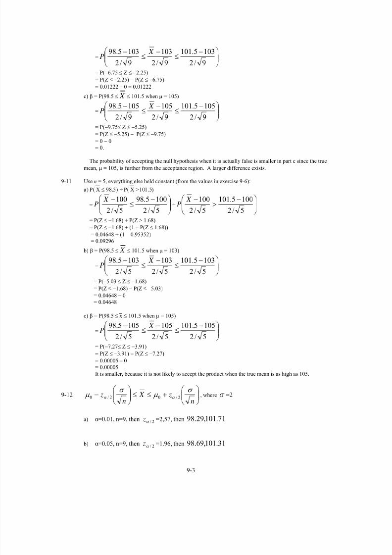
7/12/2019 Solution Manual Stats
http://slidepdf.com/reader/full/solution-manual-stats 243/588
9-3
= ⎟⎟ ⎠
⎞⎜⎜⎝
⎛ −≤
−≤
−
9/2
1035.101
9/2
103
9/2
1035.98 X P
= P(−6.75 ≤ Z ≤ −2.25)
= P(Z ≤ −2.25) − P(Z ≤ −6.75)
= 0.01222 − 0 = 0.01222
c) β = P(98.5 ≤ X ≤ 101.5 when μ = 105)
= ⎟⎟ ⎠
⎞⎜⎜⎝
⎛ −≤
−≤
−
9/2
1055.101
9/2
105
9/2
1055.98 X P
= P(−9.75≤ Z ≤ −5.25)
= P(Z ≤ −5.25) − P(Z ≤ −9.75)
= 0 − 0
= 0.
The probability of accepting the null hypothesis when it is actually false is smaller in part c since the true
mean, μ = 105, is further from the acceptance region. A larger difference exists.
9-11 Use n = 5, everything else held constant (from the values in exercise 9-6):
a) P( X ≤ 98.5) + P( X >101.5)
= ⎟⎟ ⎠
⎞⎜⎜⎝
⎛ −≤
−
5/2
1005.98
5/2
100 X P + ⎟⎟
⎠
⎞⎜⎜⎝
⎛ −>
−
5/2
1005.101
5/2
100 X P
= P(Z ≤ −1.68) + P(Z > 1.68)
= P(Z ≤ −1.68) + (1 − P(Z ≤ 1.68))
= 0.04648 + (1 − 0.95352)
= 0.09296
b) β = P(98.5 ≤ X ≤ 101.5 when μ = 103)
= ⎟⎟ ⎠
⎞⎜⎜⎝
⎛ −≤
−≤
−
5/2
1035.101
5/2
103
5/2
1035.98 X P
= P(−5.03 ≤ Z ≤ −1.68)
= P(Z ≤ −1.68) − P(Z ≤ −5.03)= 0.04648 − 0
= 0.04648
c) β = P(98.5 ≤ x ≤ 101.5 when μ = 105)
= ⎟⎟ ⎠
⎞⎜⎜⎝
⎛ −≤
−≤
−
5/2
1055.101
5/2
105
5/2
1055.98 X P
= P(−7.27≤ Z ≤ −3.91)
= P(Z ≤ −3.91) − P(Z ≤ −7.27)
= 0.00005 − 0
= 0.00005
It is smaller, because it is not likely to accept the product when the true mean is as high as 105.
9-12 ⎟⎟ ⎠
⎞⎜⎜⎝
⎛ +≤≤⎟⎟
⎠
⎞⎜⎜⎝
⎛ −
n z X
n z
σ μ
σ μ α α 2/02/0 , where σ =2
a) α=0.01, n=9, then 2/α z =2,57, then 71.101,29.98
b) α=0.05, n=9, then 2/α z =1.96, then 31.101,69.98

7/12/2019 Solution Manual Stats
http://slidepdf.com/reader/full/solution-manual-stats 244/588
9-4
c) α=0.01, n=5, then 2/α z =2.57, then 30.102,70.97
d) α=0.05, n=5, then 2/α z =1.96, then 75.101,25.98
9-13 δ =103-100=3
δ >0 then ⎟⎟ ⎠
⎞⎜⎜⎝
⎛ −Φ=
σ
δ β α
n z 2/ , where σ =2
a) β= P(98.69< X <101.31|µ=103)=P(-6.47<Z<-2.54)=0.0055
b) β= P(98.25< X <101.75|µ=103)=P(-5.31<Z<-1.40)=0.0808
a) As n increases, β decreases
9-14 a) p-value=2(1- )( 0 Z Φ )=2(1- )9/2
10098
(
−Φ )=2(1- )3(Φ )=2(1-.99865)=0.0027
b) p-value=2(1- )( 0 Z Φ )=2(1- )9/2
100101(
−Φ )=2(1- )5.1(Φ )=2(1-.93319)=0.13362
c) p-value=2(1- )( 0 Z Φ )=2(1- )9/2
100102(
−Φ )=2(1- )3(Φ )=2(1-.99865)=0.0027
9-15 a) α = P( X > 185 when μ = 175)
=
⎟⎟ ⎠
⎞
⎜⎜⎝
⎛ −>
−
10/20
175185
10/20
175 X P
= P(Z > 1.58)
= 1 − P(Z ≤ 1.58)
= 1 − 0.94295
= 0.05705
b) β = P( X ≤ 185 when μ = 185)
= ⎟⎟ ⎠
⎞⎜⎜⎝
⎛ −≤
−
10/20
185185
10/20
185 X P
= P(Z ≤ 0)
= 0.5
c) β = P( X ≤ 185 when μ = 195)
= ⎟⎟ ⎠
⎞⎜⎜⎝
⎛ −≤
−
10/20
195185
10/20
195 X P
= P(Z ≤ −1.58)
= 0.05705

7/12/2019 Solution Manual Stats
http://slidepdf.com/reader/full/solution-manual-stats 245/588
9-5
9-16 Using n = 16:
a) α = P( X > 185 when μ = 175)
= ⎟⎟ ⎠
⎞⎜⎜⎝
⎛ −>
−
16/20
175185
16/20
175 X P
= P(Z > 2)
= 1 − P(Z ≤ 2) = 1 − 0.97725 = 0.02275
b) β = P( X ≤ 185 when μ = 185)
= ⎟⎟ ⎠
⎞⎜⎜⎝
⎛ −≤
−
16/20
185185
16/20
195 X P
= P(Z ≤ 0) = 0.5.
c) β = P( X ≤ 185 when μ = 195)
= ⎟⎟ ⎠
⎞⎜⎜⎝
⎛ −≤
−
16/20
195185
16/20
195 X P
= P(Z ≤ −2) = 0.02275
9-17 ⎟⎟ ⎠
⎞⎜⎜⎝
⎛ +≥
n Z X
20175 α
a) α=0.01, n=10, then α z =2.32 and critical value is 189.67
b) α=0.05, n=10, then α z =1.64 and critical value is 185.93
c) α=0.01, n=16, then α z = 2.32 and critical value is 186.6
d) α=0.05, n=16, then α z =1.64 and critical value is 183.2
9-18 a) α=0.05, n=10, then the critical value 185.93 (from 9-17 part (b))
β = P( X ≤ 185.37 when μ = 185)
= ⎟⎟ ⎠
⎞⎜⎜⎝
⎛ −≤
−
10/20
18593.185
10/20
185 X P
= P(Z ≤ 0.147)
= 0.5584
b) α=0.05, n=16, then the critical value 183.2 (from 9-17(d)), then
β = P( X ≤ 183.2 when μ = 185)
= ⎟⎟ ⎠ ⎞
⎜⎜⎝ ⎛ −≤−
16/20
1852.183
16/20
185 X P
= P(Z ≤ -0.36)
= 0.3594
c) as n increases, β decreases

7/12/2019 Solution Manual Stats
http://slidepdf.com/reader/full/solution-manual-stats 246/588
9-6
9-19 p-value=1- )( 0 Z Φ ) wheren
X Z
/
00
σ
μ −=
a) X =180 then 79.010/20
1751800 =
−= Z
p-value=1- 2148.07852.01)79.0( =−=Φ
b) X =190 then 37.210/20
1751900 =
−= Z
p-value=1- 008894.0991106.01)37.2( =−=Φ
c) X =170 then 79.010/20
1751700 −=
−= Z
p-value=1- 785236.0214764.01)79.0( =−=−Φ
9-20 a) α = P( X ≤ 4.85 when μ = 5) + P( X > 5.15 when μ = 5)
= ⎟⎟ ⎠
⎞⎜⎜⎝
⎛ −≤−8/25.0
585.4
8/25.0
5 X P + ⎟⎟
⎠
⎞⎜⎜⎝
⎛ −>−8/25.0
515.5
8/25.0
5 X P
= P(Z ≤ −1.7) + P(Z > 1.7)
= P(Z ≤ −1.7) + (1 − P(Z ≤ 1.7)
= 0.04457 + (1 − 0.95543)
= 0.08914
b) Power = 1 − β
β = P(4.85 ≤ X ≤ 5.15 when μ = 5.1)
= ⎟⎟ ⎠
⎞⎜⎜⎝
⎛ −≤
−≤
−
8/25.0
1.515.5
8/25.0
1.5
8/25.0
1.585.4 X P
= P(−2.83 ≤ Z ≤ 0.566)
= P(Z ≤ 0.566) − P(Z ≤ −2.83)
= 0.71566 − 0.00233
= 0.71333
1 − β = 0.2867
9-21 Using n = 16:
a) α = P( X ≤ 4.85 | μ = 5) + P( X > 5.15 | μ = 5)
= ⎟⎟ ⎠
⎞⎜⎜⎝
⎛ −≤
−
16/25.0
585.4
16/25.0
5 X P + ⎟⎟
⎠
⎞⎜⎜⎝
⎛ −>
−
16/25.0
515.5
16/25.0
5 X P
= P(Z ≤ −2.4) + P(Z > 2.4)
= P(Z ≤ −2.4) +(1 − P(Z ≤ 2.4))= 2(1 − P(Z ≤ 2.4))
= 2(1 − 0.99180)
= 2(0.0082)
= 0.0164.
b) β = P(4.85 ≤ X ≤ 5.15 | μ = 5.1)
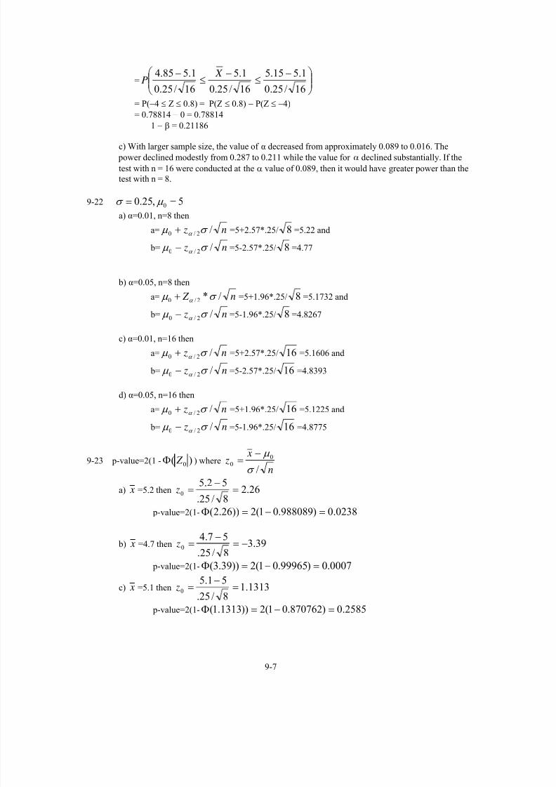
7/12/2019 Solution Manual Stats
http://slidepdf.com/reader/full/solution-manual-stats 247/588
9-7
= ⎟⎟ ⎠
⎞⎜⎜⎝
⎛ −≤
−≤
−
16/25.0
1.515.5
16/25.0
1.5
16/25.0
1.585.4 X P
= P(−4 ≤ Z ≤ 0.8) = P(Z ≤ 0.8) − P(Z ≤ −4)
= 0.78814 − 0 = 0.78814
1 − β = 0.21186
c) With larger sample size, the value of α decreased from approximately 0.089 to 0.016. The
power declined modestly from 0.287 to 0.211 while the value for α declined substantially. If the
test with n = 16 were conducted at the α value of 0.089, then it would have greater power than the
test with n = 8.
9-22 5,25.0 0 == μ σ
a) α=0.01, n=8 then
a= n z /2/0 σ μ α + =5+2.57*.25/ 8 =5.22 and
b= n z /2/0 σ μ α − =5-2.57*.25/ 8 =4.77
b) α=0.05, n=8 then
a= n Z /*2/0 σ μ α + =5+1.96*.25/ 8 =5.1732 and
b= n z /2/0 σ μ α − =5-1.96*.25/ 8 =4.8267
c) α=0.01, n=16 then
a= n z /2/0 σ μ α + =5+2.57*.25/ 16 =5.1606 and
b= n z /2/0 σ μ α − =5-2.57*.25/ 16 =4.8393
d) α=0.05, n=16 then
a= n z /2/0 σ μ α + =5+1.96*.25/ 16 =5.1225 and
b= n z /2/0 σ μ α − =5-1.96*.25/ 16 =4.8775
9-23 p-value=2(1 - )( 0 Z Φ ) wheren
x z
/
00
σ
μ −=
a) x =5.2 then 26.28/25.
52.50 =
−= z
p-value=2(1- 0238.0)988089.01(2))26.2( =−=Φ
b) x =4.7 then 39.38/25.
57.40 −=
−= z
p-value=2(1- 0007.0)99965.01(2))39.3( =−=Φ
c) x =5.1 then 1313.18/25.
51.50 =
−= z
p-value=2(1- 2585.0)870762.01(2))1313.1( =−=Φ

7/12/2019 Solution Manual Stats
http://slidepdf.com/reader/full/solution-manual-stats 248/588
9-8
9-24 a) β= P(4.845< X <5.155|µ=5.05)=P(-2.59<Z<1.33)=0.9034
b) β= P(4.8775< X <5.1225|µ=5.05)=P(-2.76<Z<1.16)=0.8741
c) As the n increases, β decreases
9-25 X ~ bin(15, 0.4) H 0: p = 0.4 and H 1: p ≠ 0.4
p1= 4/15 = 0.267 p2 = 8/15 = 0.533
Accept Region: 533.0ˆ267.0 ≤≤ p
Reject Region: 267.0ˆ < p or 533.0ˆ > p
Use the normal approximation for parts a) and b)
a) When p = 0.4, )533.0ˆ()267.0ˆ( >+<= pP pPα
29372.0
14686.014686.0
))05.1(1()05.1(
)05.1()05.1(
15
)6.0(4.0
4.0533.0
15
)6.0(4.0
4.0267.0
=
+=
<−+−<=
>+−<=
⎟⎟
⎟⎟
⎠
⎞
⎜⎜
⎜⎜
⎝
⎛ −
>+
⎟⎟
⎟⎟
⎠
⎞
⎜⎜
⎜⎜
⎝
⎛ −
<=
Z P Z P
Z P Z P
Z P Z P
b) When p = 0.2,
⎟⎟⎟⎟
⎟
⎠
⎞
⎜⎜⎜⎜
⎜
⎝
⎛
−≤≤−=≤≤=
15
)8.0(2.02.0533.0
15
)8.0(2.02.0267.0)533.0ˆ267.0( Z P pP β
2572.0
74215.099936.0
)65.0()22.3(
)22.365.0(
=
−=
≤−≤=
≤≤=
Z P Z P
Z P
9-26 X ~ bin(10, 0.3) Implicitly, H 0: p = 0.3 and H1: p < 0.3
n = 10
Accept region: 1.0ˆ > p
Reject region: 1.0ˆ ≤ p
Use the normal approximation for parts a), b) and c):
a) When p =0.3 α = ( )⎟⎟⎟⎟
⎠
⎞
⎜⎜⎜⎜
⎝
⎛ −
≤=<
10
)7.0(3.0
3.01.01.0ˆ Z P pP

7/12/2019 Solution Manual Stats
http://slidepdf.com/reader/full/solution-manual-stats 249/588
9-9
08379.0
)38.1(
=
−≤= Z P
b) When p = 0.2 β = ( ) ⎟⎟⎟⎟
⎠
⎞
⎜⎜⎜⎜
⎝
⎛ −
>=>10
)8.0(2.0
2.01.0
1.0ˆ Z P pP
78524.0
)79.0(1
)79.0(
=
−<−=
−>=
Z P
Z P
c) Power = 1 − β = 1 − 078524 = 0.21476
9-27 The problem statement implies H 0: p = 0.6, H 1: p > 0.6 and defines an acceptance region as
80.0500
400ˆ =≤ p and rejection region as 80.0ˆ > p
a) α=P( p̂ >0.80 | p=0.60) = P
⎟⎟⎟⎟
⎠
⎞
⎜⎜⎜⎜
⎝
⎛ −
>
500
)4.0(6.0
60.080.0 Z
= P(Z>9.13)=1-P(Z≤ 9.13) ≈ 0
b) β = P( p̂ ≤ 0.8 when p=0.75) = P(Z ≤ 2.58)=0.99506
9-28 a) Operating characteristic curve:
x
P Zx
P Z
=
= ≤−⎛
⎝ ⎜⎞
⎠⎟ = ≤−⎛
⎝ ⎜⎞
⎠⎟
185
20 10
185
20 10βμ μ
/ /
μ P Z ≤−⎛
⎝ ⎜
⎞
⎠⎟
185
20 10
μ
/= β 1 − β
178 P(Z ≤ 1.11) = 0.8665 0.1335
181 P(Z ≤ 0.63) = 0.7357 0.2643
184 P(Z ≤ 0.16) = 0.5636 0.4364
187 P(Z ≤ −0.32) = 0.3745 0.6255
190 P(Z ≤ −0.79) = 0.2148 0.7852
193 P(Z ≤ −1.26) = 0.1038 0.8962
196 P(Z ≤ −1.74) = 0.0409 0.9591
199 P(Z ≤ −2.21) = 0.0136 0.9864

7/12/2019 Solution Manual Stats
http://slidepdf.com/reader/full/solution-manual-stats 250/588
175 180 185 190 195 200
μ
0
0.2
0.4
0.6
0.8
1
β
Operating Characteristic Curve
b)
175 180 185 190 195 200
μ
0
0.2
0.4
0.6
0.8
1
1 − β
Power Function Curve

7/12/2019 Solution Manual Stats
http://slidepdf.com/reader/full/solution-manual-stats 251/588
9-10
Section 9-2
9-29 a) 10:,10: 10 >= μ μ H H
b) 7:,7: 10 ≠= μ μ H H
c) 5:,5: 10 <= μ μ H H
9-30 a) α=0.01, then a= 2/α z =2.57 and b=- 2/α z =-2.57
b) α=0.05, then a= 2/α z =1.96 and b=- 2/α z =-1.96
c) α=0.1, then a=2/α
z =1.65 and b=-2/α
z =-1.65
9-31 a) α=0.01, then a= α z ≅ 2.33
b) α=0.05, then a= α z ≅ 1.64

7/12/2019 Solution Manual Stats
http://slidepdf.com/reader/full/solution-manual-stats 252/588
9-11
c) α=0.1, then a= α z ≅ 1.29
9-32 a) α=0.01, then a= α −1 z ≅ -2.33
b) α=0.05, then a= α −1 z ≅ -1.64
c) α=0.1, then a=α −1
z ≅ -1.29
9-33 a) p-value=2(1- )( 0 Z Φ )=2(1- )05.2(Φ ) ≅ 0.04
b) p-value=2(1- )( 0 Z Φ )=2(1- )84.1(Φ ) ≅ 0.066
c) p-value=2(1- )( 0 Z Φ )=2(1- )4.0(Φ ) ≅ 0.69
9-34 a) p-value=1- )( 0 Z Φ =1- )05.2(Φ ≅ 0.02
b) p-value=1- )( 0 Z Φ =1- )84.1(−Φ ≅ 0.97
c) p-value=1- )( 0 Z Φ =1- )4.0(Φ ≅ 0.34
9-35 a) p-value= )( 0 Z Φ = )05.2(Φ ≅ 0.98
b) p-value= )( 0 Z Φ = )84.1(−Φ ≅ 0.03
c) p-value= )( 0 Z Φ = )4.0(Φ ≅ 0.65
9-36 a.) 1) The parameter of interest is the true mean water temperature, μ.
2) H0 : μ = 100
3) H1 : μ > 100
4) α = 0.05
5) zx
n0 =
− μ
σ /
6) Reject H0 if z0 > zα where z0.05 = 1.65
7) 98= x , σ = 2
0.39/2
100980 −=
−= z
8) Since -3.0 < 1.65 do not reject H0 and conclude the water temperature is not significantly different
greater than 100 at α = 0.05.
b) P-value = 99865.000135.01)0.3(1 =−=−Φ−
c) ⎟⎟ ⎠
⎞⎜⎜⎝
⎛ −+Φ=
9/2
10410005.0 z β
= Φ(1.65 + −6)
= Φ(-4.35)
≅0
9-37 a) 1) The parameter of interest is the true mean crankshaft wear, μ.
2) H0 : μ = 3
3) H1 : μ ≠ 3
4) α = 0.05
5) zx
n0 =
− μ
σ /
6) ) Reject H0 if z0 < −z α/2 where −z0.025 = −1.96 or z0 > zα/2 where z0.025 = 1.96

7/12/2019 Solution Manual Stats
http://slidepdf.com/reader/full/solution-manual-stats 253/588
9-12
7) x = 2.78, σ = 0.9
95.015/9.0
378.20 −=
−= z
8) Since –0.95 > -1.96, do not reject the null hypothesis and conclude there is not sufficient evidence
to support the claim the mean crankshaft wear is not equal to 3 at α = 0.05.
b) ⎟⎟ ⎠ ⎞⎜⎜⎝ ⎛ −+−Φ−⎟⎟ ⎠ ⎞⎜⎜⎝ ⎛ −+Φ= 15/9.025.33
15/9.025.33 025.0025.0 z z β
= Φ(1.96 + −1.08) − Φ(−1.96 + −1.08)
= Φ(0.88) − Φ(-3.04)
= 0.81057 − (0.00118)
= 0.80939
c)( ) ( )
,21.15)75.0(
)9.0()29.196.1(
)375.3( 2
22
2
22
10.0025.0
2
22
2/ =+
=−
+=
+=
σ
δ
σ β α z z z zn 16≅n
9-38 a) 1) The parameter of interest is the true mean melting point, μ.
2) H0 : μ = 155
3) H1 : μ ≠ 155
4) α = 0.01
5) zx
n0 =
− μ
σ /
6) Reject H0 if z0 < −z α/2 where −z0.005 = −2.58 or z0 > zα/2 where z0.005 = 2.58
7) x = 154.2, σ = 1.5
69.110/5.1
1552.1540 −=
−= z
8) Since –1.69 > -2.58, do not reject the null hypothesis and conclude there is not sufficient evidence
to support the claim the mean melting point is not equal to 155 °F at α = 0.01.
b) P-value = 2*P(Z <- 1.69) =2* 0.045514 = 0.091028
c)
⎟⎟
⎠
⎞⎜⎜⎝
⎛ −−−Φ−⎟
⎟ ⎠
⎞⎜⎜⎝
⎛ −−Φ=
⎟⎟
⎠
⎞⎜⎜⎝
⎛ −−Φ−⎟
⎟ ⎠
⎞⎜⎜⎝
⎛ −Φ=
5.1
10)150155(58.2
5.1
10)150155(58.2
005.0005.0σ
δ
σ
δ β
n z
n z
= Φ(-7.96)- Φ(-13.12) = 0 – 0 = 0
d)
( ) ( ),35.1
)5(
)5.1()29.158.2(
)155150( 2
22
2
22
10.0005.0
2
22
2/ =+
=−
+=
+=
σ
δ
σ β α z z z zn
n ≅ 2.
9-39 a.) 1) The parameter of interest is the true mean battery life in hours, μ.
2) H0 : μ = 40
3) H1 : μ > 40
4) α = 0.05
5) zx
n0 =
− μ
σ /

7/12/2019 Solution Manual Stats
http://slidepdf.com/reader/full/solution-manual-stats 254/588
9-13
6) Reject H0 if z0 > zα where z0.05 = 1.65
7) 5.40= x , σ = 1.25
26.110/25.1
405.400 =
−= z
8) Since 1.26 < 1.65 do not reject H0 and conclude the battery life is not significantly different greater than
40 at α = 0.05.
b) P-value = 1038.08962.01)26.1(1 =−=Φ−
c) ⎟⎟ ⎠
⎞⎜⎜⎝
⎛ −+Φ=
10/25.1
424005.0 z β
= Φ(1.65 + −5.06)
= Φ(-3.41)
≅ 0.000325
d)( ) ( )
,844.0)4(
)25.1()29.165.1(
)4440( 2
22
2
22
10.005.0
2
22
=+
=−
+=
+=
σ
δ
σ β α z z z zn 1≅n
e) 95% Confidence Interval
μ
μ
μ σ
≤
≤+≤+
85.39
10/)25.1(65.15.40
/05.0 n z x
The lower bound of the 90 % confidence interval must be greater than 40 to verify that the true mean exceeds
40 hours.
9-40 a)
1) The parameter of interest is the true mean tensile strength, μ.
2) H0 : μ = 3500
3) H1 : μ ≠ 3500
4) α = 0.01
5) z
x
n0 =
− μ
σ /
6) Reject H0 if z0 < −zα/2 where −z0.005 = −2.58 or z0 > zα/2
where z0.005 = 2.58
7) 3450= x , σ = 60
89.212/60
350034500 −=
−= z
8) Since −-2.89 < −2.58, reject the null hypothesis and conclude the true mean tensile strength
is significantly different from 3500 at α = 0.01.
b) Smallest level of significance =
P-value = 2[1 − Φ (2.89) ]= 2[1 − .998074] = 0.004The smallest level of significance at which we are willing to reject the null hypothesis is 0.004.
c) δ = 3470 – 3500 = -30

7/12/2019 Solution Manual Stats
http://slidepdf.com/reader/full/solution-manual-stats 255/588
9-14
0.005 0.005
(3470 3500) 12 (3470 3500) 122.58 2.58
60 60
n n z z
δ δ β
σ σ
⎛ ⎞ ⎛ ⎞= Φ − − Φ − −⎜ ⎟ ⎜ ⎟
⎝ ⎠ ⎝ ⎠
⎛ ⎞ ⎛ ⎞− −= Φ − − Φ − −⎜ ⎟ ⎜ ⎟
⎝ ⎠ ⎝ ⎠
= Φ(4.312)- Φ(-0.848) = 1 – 0.1982 = 0.8018
d) zα/2 = z0.005 = 2.58
0.005 0.005 x z x zn n
σ σ μ
⎛ ⎞ ⎛ ⎞− ≤ ≤ +⎜ ⎟ ⎜ ⎟⎝ ⎠ ⎝ ⎠
60 603450 2.58 3450 2.58
12 12μ
⎛ ⎞ ⎛ ⎞− ≤ ≤ +⎜ ⎟ ⎜ ⎟
⎝ ⎠ ⎝ ⎠
3405.313≤ μ ≤ 3494.687
With 99% confidence, we believe the true mean tensile strength is between 3405.313 psi and
3494.687 psi. We can test the hypotheses that the true mean tensile strength is not equal to 3500
by noting that the value is not within the confidence interval. Hence we reject the null hypothesis.
9-41 a) 1) The parameter of interest is the true mean speed, μ.
2) H0 : μ = 100
3) H1 : μ < 100
4) α = 0.05
5) zx
n0 =
− μ
σ /
6) Reject H0 if z0 < −zα where −z0.05 = −1.65
7) 2.102= x
, σ = 4
56.18/4
1002.1020 =
−= z
8) Since 1.56> −1.65, do not reject the null hypothesis and conclude the there is insufficient
evidence to conclude that the true speed strength is less than 100 at α = 0.05.
b) 56.10 = z , then p-value= 94.0)( 0 ≅Φ z
c) ⎟⎟ ⎠
⎞⎜⎜⎝
⎛ −−−Φ−=
4
8)10095(1 05.0 z β = 1-Φ(-1.65 - −3.54) = 1-Φ(1.89) = 0.02938
Power = 1-β = 1-0.02938 = 0.97062
d) n =( ) ( )
,597.4)5(
)4()03.165.1(
)10095( 2
22
2
22
15.005.0
2
22
=+
=−
+=
+ σ
δ
σ β α z z z zn ≅ 5
e) ⎟⎟ ⎠
⎞⎜⎜⎝
⎛ +≤
n z x
σ μ 05.0

7/12/2019 Solution Manual Stats
http://slidepdf.com/reader/full/solution-manual-stats 256/588
9-15
53.104
8
465.12.102
≤
⎟⎟ ⎠
⎞⎜⎜⎝
⎛ +≤
μ
μ
Because 100 is included in the CI then we don’t have enough confidence to reject the null
hypothesis.
9-42 a) 1) The parameter of interest is the true mean hole diameter, μ.
2) H0 : μ = 1.50
3) H1 : μ ≠ 1.50
4) α = 0.01
5) zx
n0 =
− μ
σ /
6) Reject H0 if z0 < −zα/2 where −z0.005 = −2.58 or z0 > zα/2
where z0.005 = 2.58
7) 4975.1= x , σ = 0.01
25.125/01.0
50.14975.10 −=
−
= z
8) Since −2.58 < -1.25 < 2.58, do not reject the null hypothesis and conclude the true mean
hole diameter is not significantly different from 1.5 in. at α = 0.01.
b) p-value=2(1- )( 0 Z Φ )=2(1- )25.1(Φ ) ≅ 0.21
c)
⎟⎟
⎠
⎞⎜⎜⎝
⎛ −−−Φ−⎟
⎟ ⎠
⎞⎜⎜⎝
⎛ −−Φ=
⎟⎟
⎠
⎞⎜⎜⎝
⎛ −−Φ−⎟
⎟ ⎠
⎞⎜⎜⎝
⎛ −Φ=
01.0
25)5.1495.1(58.2
01.0
25)5.1495.1(58.2
005.0005.0σ
δ
σ
δ β
n z
n z
= Φ(5.08)- Φ(-0.08) = 1 – .46812 = 0.53188
power=1-β=0.46812.
d) Set β = 1 − 0.90 = 0.10
n =2
22
2/ )(
δ
σ β α z z +=
2
22
10.0005.0
)50.1495.1(
)(
−
+ σ z z ≅
2
22
)005.0(
)01.0()29.158.2(
−
+= 59.908,
n ≅ 60.
e) For α = 0.01, zα/2 = z0.005 = 2.58
⎟ ⎠
⎞
⎜⎝
⎛
+≤≤⎟ ⎠
⎞
⎜⎝
⎛
− n z xn z x
σ
μ
σ 005.0005.0
⎟⎟ ⎠
⎞⎜⎜⎝
⎛ +≤≤⎟⎟
⎠
⎞⎜⎜⎝
⎛ −
25
01.058.24975.1
25
01.058.24975.1 μ
1.4923 ≤ μ ≤ 1.5027
The confidence interval constructed contains the value 1.5, thus the true mean hole diameter
could possibly be 1.5 in. using a 99% level of confidence. Since a two-sided 99% confidence

7/12/2019 Solution Manual Stats
http://slidepdf.com/reader/full/solution-manual-stats 257/588
interval is equivalent to a two-sided hypothesis test at α = 0.01, the conclusions necessarily must
be consistent.
9-43 a) 1) The parameter of interest is the true average battery life, μ.
2) H0 : μ = 4
3) H1 : μ > 4
4) α = 0.05
5) zx
n0 =
− μ
σ /
6) Reject H0 if z0 > zα where z0.05 = 1.65
7) 05.4= x , σ = 0.2
77.150/2.0
405.40 =
−= z
8) Since 1.77>1.65, reject the null hypothesis and conclude that there is sufficient evidence
to conclude that the true average battery life exceeds 4 hours at α = 0.05.
b) p-value=1- )( 0 Z
Φ =1- )77.1(Φ ≅ 0.04
c) ⎟⎟ ⎠
⎞⎜⎜⎝
⎛ −−Φ=
2.0
50)45.4(05.0 z β = Φ(1.65 – 17.68) = Φ(-16.03) = 0
Power = 1-β = 1-0 = 1
d) n =( ) ( )
,38.1)5.0(
)2.0()29.165.1(
)45.4( 2
22
2
22
1.005.0
2
22
=+
=−
+=
+ σ
δ
σ β α z z z z
n ≅ 2
e) μ
σ
≤⎟ ⎠
⎞
⎜⎝
⎛
− n z x 05.0
μ
μ
≤
≤⎟ ⎠
⎞⎜⎝
⎛ −
003.4
50
2.065.105.4
Since the lower limit of the CI is just slightly above 4, we conclude that average life is greater
than 4 hours at α=0.05.

7/12/2019 Solution Manual Stats
http://slidepdf.com/reader/full/solution-manual-stats 258/588
9-16
Section 9-3
9-44 a) α=0.01, n=20, the critical values are 861.2±
b) α=0.05, n=12, the critical values are 201.2±
c) α=0.1, n=15, the critical values are 761.1±
9-45 a) α=0.01, n=20, the critical value = 2.539
b) α=0.05, n=12, the critical value = 1.796
c) α=0.1, n=15, the critical value = 1.345
9-46 a) α=0.01, n=20, the critical value = -2.539
b)α
=0.05, n=12, the critical value = -1.796c) α=0.1, n=15, the critical value = -1.345

7/12/2019 Solution Manual Stats
http://slidepdf.com/reader/full/solution-manual-stats 259/588
9-17
9-47 a) 05.0*2025.0*2 ≤≤ p then 1.005.0 ≤≤ p
b) 05.0*2025.0*2 ≤≤ p then 1.005.0 ≤≤ p
c) 4.0*225.0*2 ≤≤ p then 8.05.0 ≤≤ p
9-48 a) 05.0025.0 ≤≤ p b) 025.0105.01 −≤≤− p then 975.095.0 ≤≤ p
c) 4.025.0 ≤≤ p
9-49 a) 025.0105.01 −≤≤− p then 975.095.0 ≤≤ p
b) 05.0025.0 ≤≤ p
c) 25.014.01 −≤≤− p then 75.06.0 ≤≤ p
9-50 a. 1) The parameter of interest is the true mean interior temperature life, μ.
2) H0 : μ = 22.53) H1 : μ ≠ 22.5
4) α = 0.05
5)ns
xt
/0
μ −=
6) Reject H0 if |t0| > tα/2,n-1 where tα/2,n-1 = 2.776
7) 22.496= x , s = 0.378 n=5
00237.05/378.0
5.22496.220 −=
−=t
8) Since –0.00237 >- 2.776, we cannot reject the null hypothesis. There is not sufficient evidence to
conclude that the true mean interior temperature is not equal to 22.5 °C at α = 0.05.
2*0.4 <P-value < 2* 0.5 ; 0.8 < P-value <1.0 b.) The points on the normal probability plot fall along the line. Therefore, there is no evidence to
conclude that the interior temperature data is not normally distributed.
21.5 22.5 23.5
1
5
10
20
30
40
50
60
70
80
90
95
99
Data
P e r c e n t
Normal Probability Plot for tempML Estimates - 95% CI
Mean
StDev
22.496
0.338384
ML Estimates

7/12/2019 Solution Manual Stats
http://slidepdf.com/reader/full/solution-manual-stats 260/588
9-18
c.) d = 66.0378.0
|5.2275.22||| 0 =−
=−
=σ
μ μ
σ
δ
Using the OC curve, Chart VII e) for α = 0.05, d = 0.66, and n = 5, we get β ≅ 0.8 and
power of 1−0.8 = 0.2.
d) d = 66.0378.0
|5.2275.22||| 0 =−=−=σ
μ μ
σ
δ
Using the OC curve, Chart VII e) for α = 0.05, d = 0.66, and β ≅ 0.1 (Power=0.9),
40=n .
e) 95% two sided confidence interval
⎟⎟ ⎠
⎞⎜⎜⎝
⎛ +≤≤⎟⎟
⎠
⎞⎜⎜⎝
⎛ −
n
st x
n
st x 4,025.04,025.0 μ
965.22027.22
5
378.0776.2496.22
5
378.0776.2496.22
≤≤
⎟⎟ ⎠
⎞⎜⎜⎝
⎛ +≤≤⎟⎟
⎠
⎞⎜⎜⎝
⎛ −
μ
μ
We cannot conclude that the mean interior temperature is not equal to 22.5 since the value is included
inside the confidence interval.
9-51 a. 1) The parameter of interest is the true mean female body temperature, μ.
2) H0 : μ = 98.6
3) H1 : μ ≠ 98.6
4) α = 0.05
5)ns
xt
/0
μ −=
6) Reject H0 if |t0| > tα/2,n-1 where tα/2,n-1 = 2.064
7) 264.98= x , s = 0.4821 n=25
48.325/4821.0
6.98264.980 −=
−=t
8) Since 3.48 > 2.064, reject the null hypothesis and conclude that the there is sufficient evidence to
conclude that the true mean female body temperature is not equal to 98.6 °F at α = 0.05.
P-value = 2* 0.001 = 0.002
b)

7/12/2019 Solution Manual Stats
http://slidepdf.com/reader/full/solution-manual-stats 261/588
9-19
Data appear to be normally distributed.
c) d = 24.14821.0
|6.9898||| 0 =−
=−
=σ
μ μ
σ
δ
Using the OC curve, Chart VII e) for α = 0.05, d = 1.24, and n = 25, we get β ≅ 0 and
power of 1−0 ≅ 1.
d) d = 83.04821.0
|6.982.98||| 0 =−
=−
=σ
μ μ
σ
δ
Using the OC curve, Chart VII e) for α = 0.05, d = 0.83, and β ≅ 0.1 (Power=0.9), 20=n .
e) 95% two sided confidence interval
⎟ ⎠
⎞⎜⎝
⎛ +≤≤⎟
⎠
⎞⎜⎝
⎛ −
n
st x
n
st x 24,025.024,025.0 μ
463.98065.9825
4821.0064.2264.98
25
4821.0064.2264.98
≤≤
⎟
⎠
⎞⎜
⎝
⎛ +≤≤⎟
⎠
⎞⎜
⎝
⎛ −
μ
μ
We can conclude that the mean female body temperature is not equal to 98.6 since the value is not included
inside the confidence interval.
9-52 a) 1) The parameter of interest is the true mean rainfall, μ.
2) H0 : μ = 25
3) H1 : μ > 25
4) α = 0.01
5) t0 =
ns
x
/
μ −
6) Reject H0 if t0 > tα,n-1 where t0.01,19 = 2.5397) x = 26.04 s = 4.78 n = 20
t0 = 97.020/78.4
2504.26=
−
8) Since 0.97 < 2.539, do not reject the null hypothesis and conclude there is insufficient evidence to indicate
that the true mean rainfall is greater than 25 acre-feet at α = 0.01. The 0.10 < P-value < 0.25.
b) the data on the normal probability plot fall along the straight line. Therefore there is evidence
that the data are normally distributed.
97 98 99
1
5
10
20
30
4050
60
70
80
90
95
99
Data
P e r c
e n t
Normal Probability Plot for 9-31ML Estimates - 95% CI

7/12/2019 Solution Manual Stats
http://slidepdf.com/reader/full/solution-manual-stats 262/588
9-20
c) d = 42.078.4
|2527||| 0 =−
=−
=σ
μ μ
σ
δ
Using the OC curve, Chart VII h) for α = 0.01, d = 0.42, and n = 20, we get β ≅ 0.7 and
power of 1−0.7 = 0.3.
d) d = 52.078.4
|255.27||| 0 =−
=−
=σ
μ μ
σ
δ
Using the OC curve, Chart VII h) for α = 0.05, d = 0.42, and β ≅ 0.1 (Power=0.9),
75=n .
e) 99% lower confidence bound on the mean diameter
0.01,19
s x t
nμ
⎛ ⎞− ≤⎜ ⎟
⎝ ⎠
4.7826.04 2.539
20
23.326
μ
μ
⎛ ⎞− ≤⎜ ⎟
⎝ ⎠≤
Since the lower limit of the CI is less than 25, we conclude that there is insufficient evidence to indicate that
the true mean rainfall is greater than 25 acre-feet at α = 0.01.
9-53 a)
1) The parameter of interest is the true mean sodium content, μ.
2) H0 : μ = 130
3) H1 : μ ≠ 130
4) α = 0.05
5)ns
xt
/0
μ −=
403020
99
95
90
80
70
6050
40
30
20
10
5
1
Data
P e r c e n t
Normal Probability Plot for rainfallML Estimates - 95% CI
Mean
StDev
26.035
4.66361
ML Estimates

7/12/2019 Solution Manual Stats
http://slidepdf.com/reader/full/solution-manual-stats 263/588
9-21
6) Reject H0 if |t0| > tα/2,n-1 where tα/2,n-1 = 2.045
7) 753.129= x , s = 0.929 n=30
456.130/929.0
130753.1290 −=
−=t
8) Since 1.456 < 2.064, do not reject the null hypothesis and conclude that the there is not
sufficient evidence that the true mean sodium content is different from 130mg at α = 0.05.
From table V the t0 value is found between the values of 0.05 and 0.1 with 29 degrees of freedom,
so 2*0.05<P-value < 2* 0.1 Therefore, 0.1< P-value < 0.2.
b) The assumption of normality appears to be reasonable.
c) d = 538.0929.0
|1305.130||| 0 =−
=−
=σ
μ μ
σ
δ
Using the OC curve, Chart VII e) for α = 0.05, d = 0.53, and n = 30, we get β ≅ 0.2 and power
of 1−0.20 = 0.80
d) d = 11.0929.0
|1301.130||| 0 =−
=−
=σ
μ μ
σ
δ
Using the OC curve, Chart VII e) for α = 0.05, d = 0.11, and β ≅ 0.25 (Power=0.75), 100=n .
e) 95% two sided confidence interval
⎟⎟ ⎠
⎞⎜⎜⎝
⎛ +≤≤⎟⎟
⎠
⎞⎜⎜⎝
⎛ −
n
st x
n
st x 29,025.029,025.0 μ
100.130406.129
30
929.0045.2753.129
30
929.0045.2753.129
≤≤
⎟⎟ ⎠
⎞⎜⎜⎝
⎛ +≤≤⎟⎟
⎠
⎞⎜⎜⎝
⎛ −
μ
μ
132131130129128127
99
9590
80
70
60
50
40
30
20
10
5
1
Data
P e r c e n t
Normal Probability Plot for 9-33ML Estimates - 95% CI

7/12/2019 Solution Manual Stats
http://slidepdf.com/reader/full/solution-manual-stats 264/588
9-22
There is no evidence that the mean differs from 130 because that value is inside the confidence
interval.
9-54 a) In order to use t statistics in hypothesis testing, we need to assume that the underlying distribution
is normal.
1) The parameter of interest is the true mean coefficient of restitution, μ.
2) H0 : μ = 0.6353) H1 : μ > 0.635
4) α = 0.05
5) t0 =ns
x
/
μ −
6) Reject H0 if t0 > tα,n-1 where t0.05,39 = 1.685
7) x = 0.624 s = 0.013 n = 40
t0 = 35.540/013.0
635.0624.0−=
−
8) Since –5.25 < 1.685, do not reject the null hypothesis and conclude that there is not
sufficient evidence to indicate that the true mean coefficient of restitution is greater than
0.635 at α = 0.05.
The area to right of -5.35 under the t distribution is greater than 0.9995 from table V.
Minitab gives P-value = 1.
b) From the normal probability plot, the normality assumption seems reasonable:
Baseball Coeff of Restit ut ion
P e r c e n t
0.660.650.640.630.620.610.600.59
99
95
90
80
70
60
50
40
30
20
10
5
1
Probabili ty Plot of Baseball Coeff of Restit utionNormal
c) d = 38.0013.0
|635.064.0||| 0 =−
=−
=σ
μ μ
σ
δ
Using the OC curve, Chart VII g) for α = 0.05, d = 0.38, and n = 40, we get β ≅ 0.25 and power
of 1−0.25 = 0.75.
d) d = 23.0013.0
|635.0638.0||| 0 =−
=−
=σ
μ μ
σ
δ
Using the OC curve, Chart VII g) for α = 0.05, d = 0.23, and β ≅ 0.25 (Power=0.75),
40=n .

7/12/2019 Solution Manual Stats
http://slidepdf.com/reader/full/solution-manual-stats 265/588
9-23
e) Lower confidence bound is 6205.01, =⎟ ⎠
⎞⎜⎝
⎛ − −
n
st x nα
Since 0.635 > 0.6205, then we fail to reject the null hypothesis.
9-55 a) In order to use t statistics in hypothesis testing, we need to assume that the underlying distribution
is normal.1) The parameter of interest is the true mean oxygen concentration, μ.
2) H0 : μ = 4
3) H1 : μ ≠ 4
4) α = 0.01
5) t0 =ns
x
/
μ −
6) Reject H0 if |t0 |>tα/2, n-1 = t0.005, 19 = 2.861
7) ⎯ x = 3.265, s = 2.127, n = 20
t0 = 55.120/127.2
4265.3−=
−
8) Because -2.861<-1.55 do not reject the null hypothesis and conclude that there isinsufficient evidence to indicate that the true mean oxygen differs from 4 at α = 0.01.
P-Value: 2*0.05<P-value<2*0.10 therefore 0.10< P-value<0.20
b) From the normal probability plot, the normality assumption seems reasonable:
O2 concentr ation
P e r c
e n t
7.55.02.50.0
99
95
90
80
70
60
50
40
30
20
10
5
1
Probabili ty Plot of O2 concentrationNormal
c.) d = 47.0127.2
|43||| 0 =−
=−
=σ
μ μ
σ
δ
Using the OC curve, Chart VII f) for α = 0.01, d = 0.47, and n = 20, we get β ≅ 0.70 and power of 1−0.70 = 0.30.
d) d = 71.0127.2
|45.2||| 0 =−
=−
=σ
μ μ
σ
δ
Using the OC curve, Chart VII f) for α = 0.01, d = 0.71, and β ≅ 0.10 (Power=0.90), 40=n .
e) The 95% confidence interval is:

7/12/2019 Solution Manual Stats
http://slidepdf.com/reader/full/solution-manual-stats 266/588
9-24
⎟ ⎠
⎞⎜⎝
⎛ +≤≤⎟
⎠
⎞⎜⎝
⎛ − −−
n
st x
n
st x nn 1,2/1,2/ α α μ = 62.49.1 ≤≤ μ
Because 4 is within the confidence interval, we fail to reject the null hypothesis.
9-56 a)
1) The parameter of interest is the true mean sodium content, μ.
2) H0 : μ = 300
3) H1 : μ > 300
4) α = 0.05
5)ns
xt
/0
μ −=
6) Reject H0 if t0 > tα,n-1 where tα,n-1 = 1.943
7) 315= x , s = 16 n=7
48.27/16
3003150 =
−=t
8) Since 2.48>1.943, reject the null hypothesis and conclude that there is sufficient evidence that
the leg strength exceeds 300 watts at α = 0.05.
The p-value is between .01 and .025
b) d = 3125.016
|300305||| 0 =−
=−
=σ
μ μ
σ
δ
Using the OC curve, Chart VII g) for α = 0.05, d = 0.3125, and n = 7,
β ≅ 0.9 and power = 1−0.9 = 0.1.
c) if 1-β>0.9 then β<0.1 and n is approximately 100
d) Lower confidence bound is 2.3031, =⎟ ⎠
⎞
⎜⎝
⎛
− − n
s
t x nα
because 300< 303.2 reject the null hypothesis
9-57 a.)1) The parameter of interest is the true mean tire life, μ.
2) H0 : μ = 60000
3) H1 : μ > 60000
4) α = 0.05
5) t0 =
ns
x
/
μ −
6) Reject H0 if t0 > tα,n-1 where 753.115,05.0 =t
7) 94.36457.139,6016 === s xn
t0 = 15.016/94.3645
600007.60139=−
8) Since 0.15 < 1.753., do not reject the null hypothesis and conclude there is insufficient evidence to indicate
that the true mean tire life is greater than 60,000 kilometers at α = 0.05. The P-value > 0.40.
b.) d = 27.094.3645
|6000061000||| 0 =−
=−
=σ
μ μ
σ
δ
Using the OC curve, Chart VII g) for α = 0.05, d = 0.27, and β ≅ 0.1 (Power=0.9),

7/12/2019 Solution Manual Stats
http://slidepdf.com/reader/full/solution-manual-stats 267/588
9-25
4=n .
Yes, the sample size of 16 was sufficient.
9-58 In order to use t statistics in hypothesis testing, we need to assume that the underlying distribution is normal.
1) The parameter of interest is the true mean impact strength, μ.
2) H0 : μ = 1.0
3) H1 : μ > 1.0
4) α = 0.05
5) t0 =
ns
x
/
μ −
6) Reject H0 if t0 > tα,n-1 where t0.05,19 = 1.729
7) x = 1.25 s = 0.25 n = 20
t0 = 47.420/25.0
0.125.1=
−
8) Since 4.47 > 1.729, reject the null hypothesis and conclude there is sufficient evidence to indicate that the
true mean impact strength is greater than 1.0 ft-lb/in at α = 0.05. The P-value < 0.0005
9-59 In order to use t statistic in hypothesis testing, we need to assume that the underlying distribution is normal.
1) The parameter of interest is the true mean current, μ.2) H0 : μ = 300
3) H1 : μ > 300
4) α = 0.05
5) t0 =
ns
x
/
μ −
6) Reject H0 if t0 > tα,n-1 where 833.19,05.0 =t
7) 7.152.31710 === s xn
t0 = 46.310/7.15
3002.317=
−
8) Since 3.46 > 1.833, reject the null hypothesis and conclude there is sufficient evidence to indicate that the
true mean current is greater than 300 microamps at α = 0.05. The 0.0025 <P-value < 0.005
9-60 a)
1) The parameter of interest is the true mean height of female engineering students, μ.
2) H0 : μ = 65
3) H1 : μ > 65
4) α = 0.05
5) t0 =ns
x
/
μ −
6) Reject H0 if t0 > tα,n-1 where t0.05,36 =1.68
7) 65.811= x inches 2.106=s inches n = 37
t0 = 34.237/11.2
65811.65=
−
8) Since 2.34 > 1.68, reject the null hypothesis and conclude that there is sufficient evidence to
indicate that the true mean height of female engineering students is not equal to 65 at α = 0.05.
P-value: 0.01<P-value<0.025.
b.) From the normal probability plot, the normality assumption seems reasonable:

7/12/2019 Solution Manual Stats
http://slidepdf.com/reader/full/solution-manual-stats 268/588
9-26
Female height s
P e r c e n t
72706866646260
99
95
90
80
70
60
50
40
30
20
10
5
1
Probabilit y Plot of Female heightsNormal
c) 42.111.2
6562 =−=d , n=37 so, from the OC Chart VII g) for α = 0.05, we find that β≅0.
Therefore, the power ≅ 1.
d.) 47.011.2
6564=
−=d so, from the OC Chart VII g) for α = 0.05, and β≅0.2 (Power=0.8).
30* =n .
9-61 a) In order to use t statistics in hypothesis testing, we need to assume that the underlying
distribution is normal.
1) The parameter of interest is the true mean distance, μ.
2) H0 : μ = 2803) H1 : μ > 280
4) α = 0.05
5) t0 =ns
x
/
μ −
6) Reject H0 if t0 > tα,n-1 where t0.05,99 =1.6604
7) x = 260.3 s = 13.41 n = 100
t0 = 69.14100/41.13
2803.260−=
−
8) Since –14.69 < 1.6604, do not reject the null hypothesis and conclude that there is
insufficient evidence to indicate that the true mean distance is greater than 280 at α = 0.05.
From table V the t0 value in absolute value is greater than the value corresponding to
0.0005. Therefore, the P-value is greater than 0.9995.
b) From the normal probability plot, the normality assumption seems reasonable:

7/12/2019 Solution Manual Stats
http://slidepdf.com/reader/full/solution-manual-stats 269/588
9-27
Dist ance for g olf balls
P e r c e n t
310300290280270260250240230220
99.9
99
95
90
80
70
60
50
40
30
20
10
5
1
0.1
Probabil it y Plot of Distance for golf ballsNormal
c) d = 75.041.13
|280290||| 0 =−
=−
=σ
μ μ
σ
δ
Using the OC curve, Chart VII g) for α = 0.05, d = 0.75, and n = 100, β ≅ 0 and power of 1−0 =
1.
d) d = 75.041.13
|280290||| 0 =−
=−
=σ
μ μ
σ
δ
Using the OC curve, Chart VII g) for α = 0.05, d = 0.75, and β ≅ 0.20 (Power=0.80), 15=n .
9-62 a) In order to use t statistics in hypothesis testing, we need to assume that the underlyingdistribution is normal.
1) The parameter of interest is the true mean concentration of suspended solids, μ.
2) H0 : μ = 55
3) H1 : μ ≠ 55
4) α = 0.05
5) t0 =ns
x
/
μ −
6) Reject H0 if |t0 | > tα/2,n-1 where t0.025,59 =2.000
7) x = 59.87 s = 12.50 n = 60
t0 = 018.3
60/50.12
5587.59=
−
8) Since 3.018 > 2.000, reject the null hypothesis and conclude that there is sufficient evidence to
indicate that the true mean concentration of suspended solids is not equal to 55 at α = 0.05.
From table V the t0 value is between the values of 0.001 and 0.0025 with 59 degrees of freedom.
Therefore 2*0.001<P-value < 2* 0.0025 and 0.002< P-value<0.005. Minitab gives a P-value of
0.0038.
b) From the normal probability plot, the normality assumption seems reasonable:

7/12/2019 Solution Manual Stats
http://slidepdf.com/reader/full/solution-manual-stats 270/588
9-28
Concentr ation of solids
P e r c e n t
1009080706050403020
99.9
99
95
90
80
70
60
50
40
30
20
10
5
1
0.1
Probabil it y Plot of Concentrati on of solidsNormal
d) 4.050.12
5550
=−
=d , n=60 so, from the OC Chart VII e) for α = 0.05, d= 0.4 and n=60 we
find that β≅0.2. Therefore, the power = 1-0.2 = 0.8.
e) From the same OC chart, and for the specified power, we would need approximately 75
observations.
4.050.12
5550=
−=d Using the OC Chart VII e) for α = 0.05, d = 0.4, and β ≅ 0.10 so
that power=0.90, 75=n .
.

7/12/2019 Solution Manual Stats
http://slidepdf.com/reader/full/solution-manual-stats 271/588
9-29
Section 9-4
9-63 a) α=0.01, n=20, from table V we find the following critical values 6.84 and 38.58
b) α=0.05, n=12, from table V we find the following critical values 3.82 and 21.92
c) α=0.10, n=15, from table V we find the following critical values 6.57 and 23.68
9-64 a) α=0.01, n=20, from table V we find =−
2
1,nα χ 36.19
b) α=0.05, n=12, from table V we find =−
2
1,nα χ 19.68
c) α=0.10, n=15, from table V we find =−
2
1,nα χ 21.06
9-65 a) α=0.01, n=20, from table V we find =−−
2
1,1 nα χ 7.63
b) α=0.05, n=12, from table V we find =−−
2
1,1 nα χ 4.57
c) α=0.10, n=15, from table V we find =−−
2
1,1 nα χ 7.79
9-66 a) 2(0.1)<P-value<2(0.5), then 0.2<P-value<1 b) 2(0.1)<P-value<2(0.5), then 0.2<P-value<1
c) 2(0.05)<P-value<2(0.1), then 0.1<P-value<0.2
9-67 a) 0.1<1-P<0.5 then 0.5<P-value<0.9
b) 0.1<1-P<0.5 then 0.5<P-value<0.9
c) 0.99<1-P<0.995 then 0.005<P-value<0.01
9-68 a) 0.1<P-value<0.5
b) 0.1<P-value<0.5
c) 0.99<P-value<0.995
9-69
a) In order to use the χ2 statistic in hypothesis testing and confidence interval construction, we needto assume that the underlying distribution is normal.
1) The parameter of interest is the true standard deviation of performance time σ. However,
the answer can be found by performing a hypothesis test on σ2.
2) H0 : σ2 = .752
3) H1 : σ2 >.752
4) α = 0.05
5) χ02 =
( )n s− 1 2
2σ
6) Reject H0 if 2
1,
2
0 −>nα χ χ where 30.262
16,05.0 = χ
7) n = 17, s = 0.09
χ02 = 23.0
75.)09.0(16)1(
2
2
2
2
==−σ
sn
8) Because 0.23 < 26.30 do not reject H0 and conclude there is insufficient evidence to indicate
the true variance of performance time content exceeds 0.752 at α = 0.05.
P-value: Because χ02 =0.23 the P-value>0.995
b) The 95% one sided confidence interval given below, includes the value 0.75. Therefore, we are
not be able to conclude that the standard deviation is greater than 0.75.

7/12/2019 Solution Manual Stats
http://slidepdf.com/reader/full/solution-manual-stats 272/588
9-30
σ
σ
≤
≤
07.0
3.26
)09(.16 22
9-70
a) In order to use the χ2
statistic in hypothesis testing and confidence interval construction, we needto assume that the underlying distribution is normal.
1) The parameter of interest is the true measurement standard deviation σ. However, the
answer can be found by performing a hypothesis test on σ2.
2) H0 : σ2 = .012
3) H1 : σ2 ≠ .012
4) α = 0.05
5) χ02 =
( )n s− 12
2σ
6) Reject H0 if χ χ α02
1 2 12< − −/ ,n where 63.52
14,975.0 = χ or χ χα02
2 12> −, ,n where
12.262
14,025.0 = χ
7) n = 15, s = 0.0083
χ02 = 6446.9
01.
)0083(.14)1(2
2
2
2
==−
σ
sn
8) Since 5.63 < 9.64 < 26.12 do not reject H0
P-value: 0.1<P-value/2<0.5. Therefore, 0.2<P-value<1
b) The 95% confidence interval includes the value 0.01. Therefore, there is not enough evidence
to reject the null hypothesis.
013.000607.0
63.5
)0083(.14
12.26
)0083(.14
2
22
2
≤≤
≤≤
σ
σ
9-71
a) In order to use the χ2 statistic in hypothesis testing and confidence interval construction, we need
to assume that the underlying distribution is normal.
1) The parameter of interest is the true standard deviation of titanium percentage, σ. However,
the answer can be found by performing a hypothesis test on σ2.
2) H0 : σ2 = (0.25)2
3) H1 : σ2 ≠ (0.25)2
4) α = 0.05
5) χ02 =
( )n s− 1 2
2σ
6) Reject H0 if χ χ α02
1 2 12
< − −/ ,n where χ0 995 502. , = 32.36 or χ χα0
22 1
2
> −, ,n where
χ0 005 502. , = 71.42
7) n = 51, s = 0.37
χ02 =
( ) ( . )
( . ).
n s−= =
1 50 0 37
0 25109 52
2
2
2
2σ
8) Since 109.52 > 71.42 we reject H0 and conclude there is sufficient evidence to indicate the
true standard deviation of titanium percentage is significantly different from 0.25 at α = 0.01.

7/12/2019 Solution Manual Stats
http://slidepdf.com/reader/full/solution-manual-stats 273/588
9-31
P-value: p/2<.005 then p<0.01
b) 95% confidence interval for σ:
First find the confidence interval for σ2 :
For α = 0.05 and n = 51, χα / ,2 12
n− = χ0 025 502. , = 71.42 and χ α1 2 1
2− − =/ ,n χ0 975 50
2. , = 32.36
36.32)37.0(50
42.71)37.0(50
2
2
2
≤≤ σ
0.096 ≤ σ2 ≤ 0.2115
Taking the square root of the endpoints of this interval we obtain,
0.31 < σ < 0.46
Since 0.25 falls below the lower confidence bound we would conclude that the population
standard deviation is not equal to 0.25.
9-72
a) In order to use the χ2 statistic in hypothesis testing and confidence interval construction, we need to
assume that the underlying distribution is normal.
1) The parameter of interest is the true standard deviation of Izod impact strength, σ. However, the
answer can be found by performing a hypothesis test on σ2.
2) H0 : σ2
= (0.10)2
3) H1 : σ
2 ≠ (0.10)2
4) α = 0.01
5) χ02 =
( )n s− 1 2
2σ
6) Reject H0 if χ χ α02
1 2 12< − −/ ,n where 84.62
19,995.0 = χ 27 or χ χα02
2 12> −, ,n where 58.382
19,005.0 = χ
7) n = 20, s = 0.25
χ02 = 75.118
)10.0(
)25.0(19)1(2
2
2
2
==−
σ
sn
8) Since 118.75 > 38.58 reject H0 and conclude there is sufficient evidence to indicate the true
standard deviation of Izod impact strength is significantly different from 0.10 at α = 0.01.
b.)P
-value: The P-value<0.005
c.) 99% confidence interval for σ:
First find the confidence interval for σ2
:
For α = 0.01 and n = 20, χα / ,2 12
n− = 84.62
19,995.0 = χ and χ α1 2 12
− − =/ ,n 58.382
19,005.0 = χ
1736.003078.0
84.6
)25.0(19
58.38
)25.0(19
2
22
2
≤≤
≤≤
σ
σ
Since 0.01 falls below the lower confidence bound we would conclude that the population standard deviation
is not equal to 0.01.
9-73a) In order to use the χ2 statistic in hypothesis testing and confidence interval construction, we need
to assume that the underlying distribution is normal.
1) The parameter of interest is the standard deviation of tire life, σ. However, the answer can
be found by performing a hypothesis test on σ2.
2) H0 : σ2 = 40002
3) H1 : σ2 <40002
4) α = 0.05

7/12/2019 Solution Manual Stats
http://slidepdf.com/reader/full/solution-manual-stats 274/588
9-32
5) χ02 =
2
2)1(
σ
sn −
6) Reject H0 if 2
1,1
2
0 −−<nα χ χ where =2
15,95.0 χ 7.26
7) n = 16, s2 = (3645.94)2
χ02 = 46.124000
)94.3645(15)1(2
2
2
2
==−
σ
sn
8) Since 12.46 > 7.26, fail to reject H0 and conclude there is not sufficient evidence to indicate
the true standard deviation of tire life is less than 4000 km at α = 0.05.
P-value = P(χ2 <12.46) for 15 degrees of freedom 0.5<1-P-value < 0.9
Then 0.1<P-value<0.5
b) The 95% one sided confidence interval below, includes the value 4000, therefore, we could not
be able to conclude that the variance was not equal to 40002.
5240
26.7
)94.3645(15 22
≤
≤
σ
σ
9-74
a) In order to use the χ2 statistic in hypothesis testing and confidence interval construction, we need to
assume that the underlying distribution is normal.
1) The parameter of interest is the true standard deviation of the diameter,σ. However, the answer can
be found by performing a hypothesis test on σ2.
2) H0 : σ2 = 0.0001
3) H1 : σ2 > 0.0001
4) α = 0.01
5) χ02
=( )n s− 1 2
2σ
6) Reject H0 if χ χα02
12> −,n where χ0 0114
2. , = 29.14
7) n = 15, s
2
= 0.008
χ02 =
( ) ( . )
..
n s−= =
1 14 0 008
000018 96
2
2
2
σ
8) Since 8.96 < 29.14 do not reject H0 and conclude there is insufficient evidence to indicate the true
standard deviation of the diameter exceeds 0.01 at α = 0.01.
P-value = P(χ2 > 8.96) for 14 degrees of freedom: 0.5 < P-value < 0.9
b) Using the chart in the Appendix, with0.015
1.50.01
λ = = and n = 15 we find β = 0.50.
c) 25.101.0
0125.0
0
===σ
σ λ power = 0.8, β=0.2
using chart VII k) the required sample size is 50
9-75
a) In order to use the χ2 statistic in hypothesis testing and confidence interval construction, we need to
assume that the underlying distribution is normal.
1) The parameter of interest is the true variance of sugar content, σ2. However, the
answer can be found by performing a hypothesis test on σ2.

7/12/2019 Solution Manual Stats
http://slidepdf.com/reader/full/solution-manual-stats 275/588
9-33
2) H0 : σ2
= 18
3) H1 : σ2 ≠ 18
4) α = 0.05
5) χ02 =
( )n s− 1 2
2σ
6) Reject H0 if χ χ α02
1 2 12< − −/ ,n where 70.22
9,975.0 = χ or χ χα02
2 12> −, ,n where 02.192
9,025.0 = χ
7) n = 10, s = 4.8
χ02 = 52.11
18
)8.4(9)1( 2
2
2
==−
σ
sn
8) Since 11.52 < 19.02 do not reject H0 and conclude there is insufficient evidence to indicate the true
variance of sugar content is significantly different from 18 at α = 0.01.
P-value: The χ02 is between 0.10 and 0.50. Therefore, 0.2<P-value<1
b) Using the chart in the Appendix, with 2λ = and n = 10 we find β = 0.45.
c) Using the chart in the Appendix, with 49.118
40==λ and β = 0.10, n = 30.

7/12/2019 Solution Manual Stats
http://slidepdf.com/reader/full/solution-manual-stats 276/588
9-34
Section 9-59-76 a)
1) The parameter of interest is the true fraction of satisfied customers.
2) H0 : p = 0.9
3) H1 : p ≠ 0.9
4) α = 0.05
5)( )00
00
1 pnp
np x z
−
−= or
( )n
p p
p p z
00
00
1
ˆ
−
−= ; Either approach will yield the
same conclusion
6) Reject H0 if z0 < − zα/2 where −zα/2 = −z0.025 = −1.96 or z0 > zα/2 where zα/2 = z0.025
= 1.96
7) x = 850 n = 1000 85.01000
850ˆ == p
( )
27.5
)1.0)(9.0(1000
)9.0(1000850
1 00
00 −=
−=
−
−=
pnp
np x z
8) Because -5.27<-1.96 reject the null hypothesis and conclude the true fraction of
satisfied customers is significantly different from 0.9 at α = 0.05.
The P-value: 2(1-Φ(5.27)) ≤ 2(1-1) ≈ 0
b) The 95% confidence interval for the fraction of surveyed customers is:
87.0827.01000
)15.0(85.096.185.
1000
)15.0(85.096.185.
)ˆ1(ˆˆ
)ˆ1(ˆˆ
2/2/
≤≤
+≤≤−
−+≤≤
−−
p
p
n
p p z p p
n
p p z p α α
Because 0.9 is not included in the confidence interval, we reject the null hypothesis at α
= 0.05.
9-77 a)
1) The parameter of interest is the true fraction of rejected parts
2) H0 : p = 0.03
3) H1 : p < 0.03
4) α = 0.05
5)( )00
00
1 pnp
np x z
−
−= or
( )n
p p
p p z
00
00
1
ˆ
−
−= ; Either approach will yield the same
conclusion
6) Reject H0 if z0 < − zα where −zα = −z0.05 = −1.65
7) x = 10 n = 500 02.0500
10ˆ == p
( )31.1
)97.0)(03.0(500
)03.0(50010
1 00
00 −=
−=
−
−=
pnp
np x z

7/12/2019 Solution Manual Stats
http://slidepdf.com/reader/full/solution-manual-stats 277/588
9-35
8) Because −1.31 > −1.65, do not reject the null hypothesis. There is not enough
evidence to conclude that the true fraction of rejected parts is significantly less than 0.03
at α = 0.05.
P-value = Φ(-1.31) = 0.095
b)
The upper one-sided 95% confidence interval for the fraction of rejected parts is:
0303.0
500
)98.0(02.065.102.
)ˆ1(ˆˆ
≤
+≤
−−≤
p
p
n
p p z p p α
Because 0.03<0.0303 the we fail to reject the null hypothesis
9-78 a)1) The parameter of interest is the true fraction defective integrated circuits
2) H0 : p = 0.05
3) H1 : p ≠ 0.05
4) α = 0.05
5)( )00
00
1 pnp
np x z
−
−= or
( )n
p p
p p z
00
00
1
ˆ
−
−= ; Either approach will yield the same
conclusion
6) Reject H0 if z0 < − zα/2 where −zα/2 = −z0.025 = −1.96 or z0 > zα/2 where zα/2 = z0.025 = 1.96
7) x = 13 n = 300 . p = =13
300
0043
( )53.0
)95.0)(05.0(300
)05.0(30013
1 00
00 −=
−=
−
−=
pnp
np x z
8) Since −0.53 > −1.65, do not reject null hypothesis and conclude the true fraction of defective
integrated circuits is not significantly less than 0.05, at α = 0.05.
The P-value: 2(1-Φ(0.53))=2(1-0.70194)=0.59612
b) The 95% confidence interval is:
065.002004.0
300
)957.0(043.096.1043
300
)957.0(043.096.1043.
)ˆ1(ˆˆ
)ˆ1(ˆˆ
2/2/
≤≤
+≤≤−
−+≤≤
−−
p
p
n
p p z p p
n
p p z p α α
Since 065.005.002004.0 ≤=≤ p , then we fail to reject the null hypothesis.
9-79 a)
1) The parameter of interest is the true success rate

7/12/2019 Solution Manual Stats
http://slidepdf.com/reader/full/solution-manual-stats 278/588
9-36
2) H0 : p = 0.78
3) H1 : p > 0.78
4) The value for α is not given. We assume α = 0.05.
5)( )00
00
1 pnp
np x z
−
−= or
( )
n
p p
p p z
00
00
1
ˆ
−
−= ; Either approach will yield the same
conclusion
6) Reject H0 if z0 > zα where zα = z0.05 = 1.65
7) x = 289 n = 350 83.0350
289ˆ ≅= p
( )06.2
)22.0)(78.0(350
)78.0(350289
1 00
00 =
−=
−
−=
pnp
np x z
8) Because 2.06 > 1.65, reject the null hypothesis and conclude the true success rate is
significantly greater than 0.78, at α = 0.05.
P-value=1-0.9803=0.0197
b) The 95% lower confidence interval:
p
p
pn
p p z p
≤
≤−
≤−
−
7969.0
350
)17.0(83.065.183.
)ˆ1(ˆˆ
α
Because 0.7969>0.78, reject the null hypothesis
9-80 a)
1) The parameter of interest is the true percentage of polished lenses that contain surface defects,
p.
2) H0 : p = 0.02
3) H1 : p < 0.02
4) α = 0.05
5)( )00
00
1 pnp
np x z
−
−= or
( )n
p p
p p z
00
00
1
ˆ
−
−= ; Either approach will yield the
same conclusion
6) Reject H0 if z0 < − zα where −zα = −z0.05 = −1.65
7) x = 6 n = 250 024.0250
6ˆ == p
( )452.0
250
)02.01(02.0
02.0024.0
1
ˆ
00
00 =
−
−=
−
−=
n
p p
p p z
8) Since 0.452 > −1.65 do not reject the null hypothesis and conclude the machine cannot be
qualified at the 0.05 level of significance.

7/12/2019 Solution Manual Stats
http://slidepdf.com/reader/full/solution-manual-stats 279/588
9-37
P-value = Φ(0.452) = 0.67364
b) The upper 95% confidence interval is:
0264.0
250
)976.0(024.065.1024.
)ˆ1(ˆ
ˆ
≤
+≤
−
+≤
p
p
n
p p
z p p α
Since 0264.002.0 ≤= p then we fail to reject the null hypothesis.
9-81 a)
1) The parameter of interest is the true percentage of football helmets that contain flaws, p.
2) H0 : p = 0.1
3) H1 : p > 0.14) α = 0.01
5)( )00
00
1 pnp
np x z
−
−= or
( )n
p p
p p z
00
00
1
ˆ
−
−= ; Either approach will yield the same
conclusion
6) Reject H0 if z0 > zα where zα = z0.01 = 2.33
7) x = 16 n = 200 08.0200
16ˆ == p
( )94.0
200
)10.01(10.0
10.008.0
1
ˆ
00
0
0 −=−
−=
−
−=
n
p p
p p z
8) Because -0.94 < 2.33 do not reject the null hypothesis. There is not enough evidence that the
proportion of football helmets with flaws exceeds 10%.
P-value = 1- Φ(-0.94) =0.8264
b) The 99% lower confidence interval:
p
p
pn
p p z p
≤
≤−
≤−
−
035.0200
)92.0(08.033.208.
)ˆ1(ˆˆ
α
Because 1.0035.0 =≤ p then we fail to reject the null hypothesis.
9-82 a) 1) The parameter of interest is the true proportion of engineering students planning graduate studies
2) H0 : p = 0.50
3) H1 : p ≠ 0.50
4) α = 0.05

7/12/2019 Solution Manual Stats
http://slidepdf.com/reader/full/solution-manual-stats 280/588
9-38
5)
( )00
0
01 pnp
np x z
−
−= or
( )n
p p
p p z
00
0
01
ˆ
−
−= ; Either approach will yield the same conclusion
6) Reject H0 if z0 < − zα/2 where −zα/2 = −z0.025 = −1.96 or z0 > zα/2 where zα/2 = z0.025 = 1.96
7) x = 117 n = 484 2423.0484
117
ˆ == p
( )36.11
)5.0)(5.0(484
)5.0(484117
1 00
0
0 −=−
=−
−=
pnp
np x z
8) Since −11.36 > −1.65, reject the null hypothesis and conclude the true proportion of engineering students
planning graduate studies is significantly different from 0.5, at α = 0.05.
P-value =2[1 − Φ(11.36)] ≅ 0
b.) 242.0484
117ˆ == p
280.0204.0
484
)758.0(242.096.1242.0
484
)758.0(242.096.1242.0
)ˆ1(ˆˆ)ˆ1(ˆˆ 2/2/
≤≤
−≤≤−
−+≤≤−−
p
p
n p p z p p
n p p z p α α
Since the 95% confidence interval does not contain the value 0.5, then conclude that the true proportion of
engineering students planning graduate studies is significantly different from 0.5.
9-83 1) The parameter of interest is the true proportion of batteries that fail before 48 hours, p.
2) H0 : p = 0.002
3) H1 : p < 0.002
4) α = 0.01
5)( )00
00
1 pnp
np x z
−
−= or
( )n
p p
p p z
00
00
1
ˆ
−
−= ; Either approach will yield the same conclusion
6) Reject H0 if z0 < -zα where -zα = -z0.01 = -2.33
7) x = 15 n = 5000 003.05000
15ˆ == p
( )58.1
5000
)998.01(002.0
002.0003.0
1
ˆ
00
00 =
−
−=
−
−=
n
p p
p p z
8) Since 1.58 > -2.33 do not reject the null hypothesis and conclude the proportion of proportion
of cell phone batteries that fail is not less than 0.2% at α=0.01.

7/12/2019 Solution Manual Stats
http://slidepdf.com/reader/full/solution-manual-stats 281/588
9-39
9-84. The problem statement implies that H0: p = 0.6, H1: p > 0.6 and defines an acceptance region as
. p ≤ =315
5000 63 and rejection region as . p > 0 63
a) The probability of a type 1 error is
( ) ( ) 08535.0)37.1(137.1
500)4.0(6.0
6.063.06.0|63.0ˆ =<−=≥=
⎟⎟
⎟⎟
⎠
⎞
⎜⎜
⎜⎜
⎝
⎛ −
≥==≥= Z P Z P Z P p pPα .
b) β = P( P ≤ 0.63 | p = 0.75) = P(Z ≤ −6.196) = 0.
9-85 a) The parameter of interest is the true proportion of engine crankshaft bearings exhibiting surface roughness.
2) H0 : p = 0.10
3) H1 : p > 0.10
4) α = 0.05
5)
( )00
00
1 pnp
np x z
−
−= or
( )n
p p
p p z
00
00
1
ˆ
−
−= ; Either approach will yield the same conclusion
6) Reject H0 if z0 > zα where zα = z0.05 = 1.65
7) x = 10 n = 85 118.085
10ˆ == p
( )54.0
)90.0)(10.0(85
)10.0(8510
1 00
00 =
−=
−
−=
pnp
np x z
8) Because 0.54 < 1.65, do not reject the null hypothesis. There is not enough evidence to conclude that
the true proportion of crankshaft bearings exhibiting surface roughness exceeds 0.10, at α = 0.05.
P-value = 1 – Φ(0.54) = 0.295
b) p= 0.15, p0=0.10, n=85, and zα/2=1.96
639.00016.06406.0)94.2()36.0(
85/)15.01(15.0
85/)10.01(10.096.115.010.0
85/)15.01(15.0
85/)10.01(10.096.115.010.0
/)1(
/)1(
/)1(
/)1( 002/0002/0
=−=−Φ−Φ=
⎟⎟
⎠
⎞
⎜⎜
⎝
⎛
−
−−−Φ−
⎟⎟
⎠
⎞
⎜⎜
⎝
⎛
−
−+−Φ=
⎟⎟ ⎠
⎞
⎜⎜⎝
⎛
−
−−−
Φ−⎟⎟ ⎠
⎞
⎜⎜⎝
⎛
−
−+−
Φ= n p p
n p p z p p
n p p
n p p z p p α α
β
11863.117)85.10(
10.015.0
)15.01(15.028.1)10.01(10.096.1
)1()1(
2
2
2
0
002/
≅==
⎟⎟
⎠
⎞
⎜⎜
⎝
⎛
−
−−−=
⎟⎟
⎠
⎞
⎜⎜
⎝
⎛
−
−−−=
p p
p p z p p zn
β α

7/12/2019 Solution Manual Stats
http://slidepdf.com/reader/full/solution-manual-stats 282/588
9-40
Section 9-7
9-86 Expected Frequency is found by using the Poisson distribution
!)(
x
e x X P
xλ λ −
== where 41.1100/)]4(4)11(3)31(2)30(1)24(0[ =++++=λ
Value 0 1 2 3 4
Observed Frequency 24 30 31 11 4
Expected Frequency 30.12 36.14 21.69 8.67 2.60
Since value 4 has an expected frequency less than 3, combine this category with the previous category:
Value 0 1 2 3-4
Observed Frequency 24 30 31 15
Expected Frequency 30.12 36.14 21.69 11.67
The degrees of freedom are k − p − 1 = 4 − 0 − 1 = 3
a) 1) The variable of interest is the form of the distribution for X.
2) H0: The form of the distribution is Poisson
3) H1: The form of the distribution is not Poisson4) α = 0.05
5) The test statistic is
( )∑
=
−=
k
i i
ii
E
E O
1
2
2
0 χ
6) Reject H0 if χ χo2
0 0 5 32 7 81> =. , .
7)( ) ( ) ( ) ( )
23.767.11
67.1115
69.21
69.2131
14.36
14.3630
12.30
12.30242222
2
0 =−
+−
+−
+−
= χ
8) Since 7.23 < 7.81 do not reject H0. We are unable to reject the null hypothesis that the distribution of
X is Poisson.
b) The P-value is between 0.05 and 0.1 using Table IV. From Minitab the P-value = 0.0649.
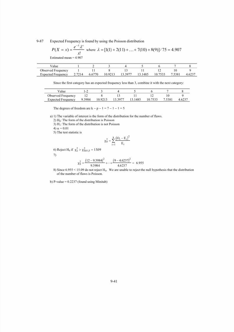
7/12/2019 Solution Manual Stats
http://slidepdf.com/reader/full/solution-manual-stats 283/588
9-41
9-87 Expected Frequency is found by using the Poisson distribution
!)(
x
e x X P
xλ λ −
== where 907.475/)]9(8)10(7)11(2)1(1[ =++++= …λ
Estimated mean = 4.907
Value 1 2 3 4 5 6 7 8
Observed Frequency 1 11 8 13 11 12 10 9
Expected Frequency 2.7214 6.6770 10.9213 13.3977 13.1485 10.7533 7.5381 4.6237
Since the first category has an expected frequency less than 3, combine it with the next category:
Value 1-2 3 4 5 6 7 8
Observed Frequency 12 8 13 11 12 10 9
Expected Frequency 9.3984 10.9213 13.3977 13.1485 10.7533 7.5381 4.6237
The degrees of freedom are k − p − 1 = 7 − 1 − 1 = 5
a) 1) The variable of interest is the form of the distribution for the number of flaws.
2) H0: The form of the distribution is Poisson
3) H1: The form of the distribution is not Poisson
4) α = 0.01
5) The test statistic is
( )χ0
22
1
=−
=∑
O E
E
i i
ii
k
6) Reject H0 if χ χo2
00152
1509> =. , .
7)
( ) ( )χ0
22 2
12 9 3984
9 3984
9 4 6237
4 6237=
−+ +
−=
.
.
.
. 6.955
8) Since 6.955 < 15.09 do not reject H0. We are unable to reject the null hypothesis that the distribution
of the number of flaws is Poisson.
b) P-value = 0.2237 (found using Minitab)

7/12/2019 Solution Manual Stats
http://slidepdf.com/reader/full/solution-manual-stats 284/588
9-42
9-88 Estimated mean = 10.131
Value 5 6 8 9 10 11 12 13 14 15
Rel. Freq 0.067 0.067 0.100 0.133 0.200 0.133 0.133 0.067 0.033 0.067
Observed
(Days)
2 2 3 4 6 4 4 2 1 2
Expected
(Days)
1.0626 1.7942 3.2884 3.7016 3.7501 3.4538 2.9159 2.2724 1.6444 1.1106
Since there are several cells with expected frequencies less than 3, the revised table would be:
Value 5-8 9 10 11 12-15
Observed
(Days)
7 4 6 4 9
Expected
(Days)
6.1452 3.7016 3.7501 3.4538 7.9433
The degrees of freedom are k − p − 1 = 5 − 1 − 1 = 3
a) 1) The variable of interest is the form of the distribution for the number of calls arriving to a switchboard
from noon to 1pm during business days.2) H0: The form of the distribution is Poisson
3) H1: The form of the distribution is not Poisson
4) α = 0.05
5) The test statistic is
( )χ0
22
1
=−
=∑
O E
E
i i
ii
k
6) Reject H0 if χ χo2
0 0 5 32 7 81> =. , .
7)
( ) ( ) ( ) ( ) ( )1.72
9433.7
9433.79
4538.3
4538.34
7501.3
7501.36
7016.3
7016.34
1452.6
1452.6722222
2
0 =−
+−
+−
+−
+−
= χ
8) Since 1.72 < 7.81 do not reject H0. We are unable to reject the null hypothesis that the distribution
for the number of calls is Poisson.
b) The P-value is between 0.9 and 0.5 using Table IV. P-value = 0.6325 (found using Minitab)

7/12/2019 Solution Manual Stats
http://slidepdf.com/reader/full/solution-manual-stats 285/588
9-43
9-89 Use the binomial distribution to get the expected frequencies with the mean = np = 6(0.25) = 1.5
Value 0 1 2 3 4
Observed 4 21 10 13 2
Expected 8.8989 17.7979 14.8315 6.5918 1.6479
The expected frequency for value 4 is less than 3. Combine this cell with value 3:
Value 0 1 2 3-4
Observed 4 21 10 15
Expected 8.8989 17.7979 14.8315 8.2397
The degrees of freedom are k − p − 1 = 4 − 0 − 1 = 3
a) 1) The variable of interest is the form of the distribution for the random variable X.
2) H0: The form of the distribution is binomial with n = 6 and p = 0.25
3) H1: The form of the distribution is not binomial with n = 6 and p = 0.25
4) α = 0.05
5) The test statistic is
( )χ0
22
1
=−
=∑
O E
E
i i
ii
k
6) Reject H0 if χ χo2
0 0 5 32 7 81> =. , .
7)
( ) ( )χ0
22 2
4 88989
88989
15 8 2397
82397=
−+ +
−=
.
.
.
. 10.39
8) Since 10.39 > 7.81 reject H0. We can conclude that the distribution is not binomial with n = 6 and p =
0.25 at α = 0.05.
b) P-value = 0.0155 (from Minitab)
9-90 The value of p must be estimated. Let the estimate be denoted by psample
sample mean =+ + +
=0 39 1 23 2 12 3 1
750 6667
( ) ( ) ( ) ( ).
02778.024
6667.0ˆ ===
n
meansample psample
Value 0 1 2 3
Observed 39 23 12 1
Expected 38.1426 26.1571 8.5952 1.8010
Since value 3 has an expected frequency less than 3, combine this category with that of value 2:
Value 0 1 2-3
Observed 39 23 13
Expected 38.1426 26.1571 10.3962
The degrees of freedom are k − p − 1 = 3 − 1 − 1 = 1
a) 1) The variable of interest is the form of the distribution for the number of underfilled cartons, X.
2) H0: The form of the distribution is binomial
3) H1: The form of the distribution is not binomial
4) α = 0.05
5) The test statistic is

7/12/2019 Solution Manual Stats
http://slidepdf.com/reader/full/solution-manual-stats 286/588
9-44
( )χ0
22
1
=−
=∑
O E
E
i i
ii
k
6) Reject H0 if χ χo2
00512 384> =. , .
7)( ) ( )
χ02
2 2 239 38 1426
381426
23 26 1571
261571
13 10 3962
1039=
−+
−+
−=
.
.
( . )
.
.
.1.053
8) Since 1.053 < 3.84 do not reject H0. We are unable to reject the null hypothesis that the distribution
of the number of underfilled cartons is binomial at α = 0.05.
b) The P-value is between 0.5 and 0.1 using Table IV. From Minitab the P-value = 0.3048.
9-91 Estimated mean = 49.6741 use Poisson distribution with λ=49.674
All expected frequencies are greater than 3.
The degrees of freedom are k − p − 1 = 26 − 1 − 1 = 24
a) 1) The variable of interest is the form of the distribution for the number of cars passing through the
intersection.
2) H0: The form of the distribution is Poisson
3) H1: The form of the distribution is not Poisson
4) α = 0.055) The test statistic is
( )χ0
22
1
=−
=∑
O E
E
i i
ii
k
6) Reject H0 if χ χo2
005242 3642> =. , .
7) Estimated mean = 49.6741
χ02 769 57= .
8) Since 769.57 >>> 36.42, reject H0. We can conclude that the distribution is not Poisson at α = 0.05.
b) P-value = 0 (found using Minitab)
9-92 The Expected Frequency is found by using the Poisson distribution
!)(
xe x X P
x
λ
λ −
== where 514.19105/)]1(41)1(39)1(7)1(6[ =++++= …λ
Estimated mean = 19.514
Number ofEarthquakes
ObservedFrequency
ExpectedFrequency
6 1 0.03
7 1 0.08
8 4 0.18
10 3 0.78
11 2 1.38
12 2 2.24
13 6 3.36
14 5 4.69
15 11 6.10
16 7 7.43
17 3 8.53
18 8 9.25
19 4 9.50
20 4 9.27

7/12/2019 Solution Manual Stats
http://slidepdf.com/reader/full/solution-manual-stats 287/588
9-45
21 7 8.62
22 8 7.64
23 4 6.48
24 3 5.27
25 2 4.12
26 4 3.0927 4 2.23
28 1 1.56
29 1 1.05
30 1 0.68
31 1 0.43
32 2 0.26
34 1 0.09
35 1 0.05
36 2 0.03
39 1 0.00
41 1 0.00
After combining categories with frequencies less than 3, we get the following table:
Number ofEarthquakes
ObservedFrequency
ExpectedFrequency
6-7-8-10-11-12 13.00 4.68
13 6 3.36
14 5 4.69
15 11 6.10
16 7 7.4317 3 8.53
18 8 9.25
19 4 9.50
20 4 9.27
21 7 8.62
22 8 7.64
23 4 6.48
24 3 5.27
25 2 4.12
26 4 3.09
27-28-29-30-31-32-34-35-36-39-41 16 6.38
The degrees of freedom are k − p − 1 = 16 − 1 − 1 = 14

7/12/2019 Solution Manual Stats
http://slidepdf.com/reader/full/solution-manual-stats 288/588
a)
1) The variable of interest is the form of the distribution for the number of earthquakes per year
of magnitude 7.0 and greater..
2) H0: The form of the distribution is Poisson
3) H1: The form of the distribution is not Poisson
4) α = 0.05
5) The test statistic is( )
χ02
2
1
=−
=∑
O E
E
i i
ii
k
6) Reject H0 if 68.232
14,05.0
2 => χ χ o
7)
( ) ( )48.89
38.6
38.616
86.4
86.41322
2
0 =−
++−
= χ
8) Since 48.89 > 23.68 reject H0. The form of the distribution of the number of earthquakes is
not Poisson.
b) P-value < 0.005

7/12/2019 Solution Manual Stats
http://slidepdf.com/reader/full/solution-manual-stats 289/588
9-46
Section 9-8
9-93 1. The variable of interest is breakdowns among shift.
2. H0: Breakdowns are independent of shift.
3. H1: Breakdowns are not independent of shift.
4. α = 0.05
5. The test statistic is:
( )∑∑
= =
−=
r
i
c
j ij
ijij
E
E O
1 1
2
2
0 χ
6. The critical value is 592.122
6,05.= χ
7. The calculated test statistic is 65.112
0
= χ
8. χ χ02
00562/>. ,
, do not reject H0 and conclude that the data provide insufficient evidence to claim that
machine breakdown and shift are dependent at α = 0.05.
P-value = 0.070 (using Minitab)
9-94 1. The variable of interest is calls by surgical-medical patients.
2. H0:Calls by surgical-medical patients are independent of Medicare status.
3. H1:Calls by surgical-medical patients are not independent of Medicare status.
4. α = 0.01
5. The test statistic is:
( )
∑∑= =
−=
r
i
c
j ij
ijij
E
E O
1 1
2
2
0
χ
6. The critical value is 637.62
1,01.= χ
7. The calculated test statistic is 033.02
0= χ
8.2
1,01.0
2
0 χ χ >/ , do not reject H0 and conclude that the evidence is not sufficient to claim that surgical-
medical patients and Medicare status are dependent. P-value = 0.85
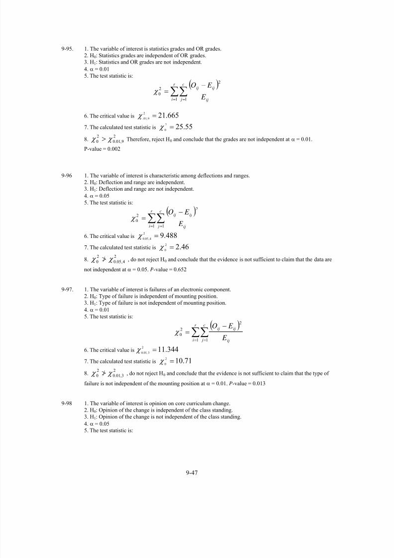
7/12/2019 Solution Manual Stats
http://slidepdf.com/reader/full/solution-manual-stats 290/588
9-47
9-95. 1. The variable of interest is statistics grades and OR grades.
2. H0: Statistics grades are independent of OR grades.
3. H1: Statistics and OR grades are not independent.
4. α = 0.01
5. The test statistic is:
( )
∑∑= =
−=
r
i
c
j ij
ijij
E
E O
1 1
2
2
0
χ
6. The critical value is 665.212
9,01.= χ
7. The calculated test statistic is 55.252
0= χ
8.2
9,01.0
2
0 χ χ > Therefore, reject H0 and conclude that the grades are not independent at α = 0.01.
P-value = 0.002
9-96 1. The variable of interest is characteristic among deflections and ranges.
2. H0: Deflection and range are independent.
3. H1: Deflection and range are not independent.
4. α = 0.05
5. The test statistic is:
( )∑∑
= =
−=
r
i
c
j ij
ijij
E
E O
1 1
2
2
0 χ
6. The critical value is 488.92
4,05.0= χ
7. The calculated test statistic is 46.22
0= χ
8.2
4,05.0
2
0 χ χ >/ , do not reject H0 and conclude that the evidence is not sufficient to claim that the data are
not independent at α = 0.05. P-value = 0.652
9-97. 1. The variable of interest is failures of an electronic component.2. H0: Type of failure is independent of mounting position.
3. H1: Type of failure is not independent of mounting position.
4. α = 0.01
5. The test statistic is:
( )∑∑
= =
−=
r
i
c
j ij
ijij
E
E O
1 1
2
2
0 χ
6. The critical value is 344.112
3,01.0= χ
7. The calculated test statistic is 71.102
0= χ
8.2
3,01.0
2
0 χ χ >/ , do not reject H0 and conclude that the evidence is not sufficient to claim that the type of
failure is not independent of the mounting position at α = 0.01. P-value = 0.013
9-98 1. The variable of interest is opinion on core curriculum change.
2. H0: Opinion of the change is independent of the class standing.
3. H1: Opinion of the change is not independent of the class standing.
4. α = 0.05
5. The test statistic is:

7/12/2019 Solution Manual Stats
http://slidepdf.com/reader/full/solution-manual-stats 291/588
( )∑∑
= =
−=
r
i
c
j ij
ijij
E
E O
1 1
2
2
0 χ
6. The critical value is 815.72
3,05.0= χ
7. The calculated test statistic is 97.262
0.= χ .
8. 23,05.0
20 χ χ >>> , reject H0 and conclude that the opinions on the change are not independent of class
standing. P-value ≈ 0
9-99 a)
1. The variable of interest is successes.
2. H0: successes are independent of size of stone.
3. H1: successes are not independent of size of stone.
4. α = 0.05
5. The test statistic is:
( )∑∑
= =
−=
r
i
c
j ij
ijij
E
E O
1 1
2
2
0 χ
6. The critical value is 84.321,05. = χ
7. The calculated test statistic2
0 χ = 13.766 with details below.
8.2
1,05.0
2
0 χ χ > , reject H0 and conclude that there is enough evidence to claim that number of
successes and the stone size are not independent.1 2 All
1 55 25 80
66.06 13.94 80.00
2 234 36 270
222.94 47.06 270.00
All 289 61 350
289.00 61.00 350.00
Cell Contents: Count
Expected count
Pearson Chi-Square = 13.766, DF = 1, P-Value = 0.000
b) P-value < 0.005

7/12/2019 Solution Manual Stats
http://slidepdf.com/reader/full/solution-manual-stats 292/588
9-48
Supplemental Exercises
9-100 α=0.01
a.) n=25 9783.0)02.2()31.033.2(25/16
868501.0 =Φ=−Φ=⎟⎟
⎠
⎞⎜⎜⎝
⎛ −+Φ= z β
n=100 9554.0)70.1()63.033.2(100/16
868501.0 =Φ=−Φ=⎟⎟
⎠
⎞⎜⎜⎝
⎛ −+Φ= z β
n=400 8599.0)08.1()25.133.2(400/16
868501.0 =Φ=−Φ=⎟⎟
⎠
⎞⎜⎜⎝
⎛ −+Φ= z β
n=2500 2119.0)80.0()13.333.2(2500/16868501.0 =−Φ=−Φ=⎟⎟
⎠ ⎞⎜⎜
⎝ ⎛ −+Φ= z β

7/12/2019 Solution Manual Stats
http://slidepdf.com/reader/full/solution-manual-stats 293/588
9-49
b) n=25 31.025/16
85860 =
−= z P-value: 3783.06217.01)31.0(1 =−=Φ−
n=100 63.0100/16
85860 =
−= z P-value: 2643.07357.01)63.0(1 =−=Φ−
n=400 25.1400/16
85860 =
−= z P-value: 1056.08944.01)25.1(1 =−=Φ−
n=2500 13.32500/16
85860 =
−= z P-value: 0009.09991.01)13.3(1 =−=Φ−
The data would be statistically significant when n=2500 at α=0.01
9-101 Sample Mean = p Sample Variance =( ) p p
n
1−
Sample Size, n Sampling Distribution Sample Mean Sample Variance
a. 50 Normal p p p( )1
50
−
b. 80 Normal p p p( )180−
c. 100 Normal p p p( )1
100
−
d) As the sample size increases, the variance of the sampling distribution decreases.
9-102
n Test statistic P-value conclusion
a. 50
12.050/)10.01(10.0
10.0095.00 −=−
−= z
0.4522 Do not reject H 0
b. 10015.0
100/)10.01(10.0
10.0095.00 −=
−
−= z
0.4404 Do not reject H 0
c. 50037.0
500/)10.01(10.0
10.0095.00 −=
−
−= z
0.3557 Do not reject H 0
d.
100053.0
1000/)10.01(10.0
10.0095.00 −=
−
−= z
0.2981 Do not reject H 0
e. The P-value decreases as the sample size increases.
9-103. σ = 12, δ = 205 − 200 = 5,α
20025= . , z0.025 = 1.96,
a) n = 20: 564.0)163.0(12
20596.1 =Φ=⎟
⎟ ⎠
⎞⎜⎜⎝
⎛ −Φ= β

7/12/2019 Solution Manual Stats
http://slidepdf.com/reader/full/solution-manual-stats 294/588
9-50
b) n = 50: 161.0839.01)986.0(1)986.0(12
50596.1 =−=Φ−=−Φ=⎟
⎟ ⎠
⎞⎜⎜⎝
⎛ −Φ= β
c) n = 100: 0116.09884.01)207.2(1)207.2(12
100596.1 =−=Φ−=−Φ=⎟
⎟ ⎠
⎞⎜⎜⎝
⎛ −Φ= β
d) β , which is the probability of a Type II error, decreases as the sample size increases because the variance
of the sample mean decreases. Consequently, the probability of observing a sample mean in the
acceptance region centered about the incorrect value of 200 ml/h decreases with larger n.
9-104 σ = 14, δ = 205 − 200 = 5,α2
0025= . , z0.025 = 1.96,
a) n = 20: 6406.0)362.0(14
20596.1 =Φ=⎟
⎟ ⎠
⎞⎜⎜⎝
⎛ −Φ= β
b) n = 50: 2877.07123.01)565.0(1)565.0(
14
50596.1 =−=Φ−=−Φ=⎟
⎟
⎠
⎞⎜⎜
⎝
⎛ −Φ= β
c) n = 100: 0537.09463.01)611.1(1)611.1(14
100596.1 =−=Φ−=−Φ=⎟
⎟ ⎠
⎞⎜⎜⎝
⎛ −Φ= β
d) The probability of a Type II error increases with an increase in the standard deviation.
9-105 σ = 8, δ = 204 − 200 = 4,α
20025= . , z0.025 = 1.96.
a) n = 20: β = −⎛
⎝ ⎜⎜
⎞
⎠⎟⎟ = − =Φ Φ196
4 20
80 28. ( . ) 1 − Φ(0.28) = 1 − 0.61026 = 0.38974
Therefore, power = 1 − β = 0.61026
b) n = 50: β = −⎛
⎝ ⎜⎜
⎞
⎠⎟⎟ = − =Φ Φ196
4 50
82 58. ( . ) 1 − Φ(2.58) = 1 − 0.99506 = 0.00494
Therefore, power = 1 − β = 0.995
c) n = 100: β = −⎛
⎝ ⎜⎜
⎞
⎠⎟⎟ = − =Φ Φ196
4 100
83 04. ( . ) 1 − Φ(3.04) = 1 − 0.99882 = 0.00118
Therefore, power = 1 − β = 0.9988
d) As sample size increases, and all other values are held constant, the power increases because the
variance of the sample mean decreases. Consequently, the probability of a Type II error decreases,
which implies the power increases.
9-106 a) α=0.05
n=100 3632.0)35.0()0.265.1(100/)5.0(5.0
6.05.005.0 =−Φ=−Φ=⎟
⎟ ⎠
⎞⎜⎜⎝
⎛ −+Φ= z β
6368.03632.011 =−=−= β Power
n=150 2119.0)8.0()45.265.1(100/)5.0(5.0
6.05.005.0 =−Φ=−Φ=⎟
⎟ ⎠
⎞⎜⎜⎝
⎛ −+Φ= z β

7/12/2019 Solution Manual Stats
http://slidepdf.com/reader/full/solution-manual-stats 295/588
9-51
7881.02119.011 =−=−= β Power
n=300 03515.0)81.1()46.365.1(300/)5.0(5.0
6.05.005.0 =−Φ=−Φ=⎟
⎟ ⎠
⎞⎜⎜⎝
⎛ −+Φ= z β
96485.003515.011 =−=−= β Power
b) α=0.01
n=100 6293.0)33.0()0.233.2(100/)5.0(5.0
6.05.001.0 =Φ=−Φ=⎟
⎟ ⎠
⎞⎜⎜⎝
⎛ −+Φ= z β
3707.06293.011 =−=−= β Power
n=150 4522.0)12.0()45.233.2(100/)5.0(5.0
6.05.001.0 =−Φ=−Φ=⎟
⎟ ⎠
⎞⎜⎜⎝
⎛ −+Φ= z β
5478.04522.011 =−=−= β Power
n=300 1292.0)13.1()46.333.2(
300/)5.0(5.0
6.05.001.0 =−Φ=−Φ=
⎟
⎟
⎠
⎞
⎜
⎜
⎝
⎛ −+Φ= z β
8702.01292.011 =−=−= β Power
Decreasing the value of α decreases the power of the test for the different sample sizes.
c) α=0.05
n=100 0.0)35.4()0.665.1(100/)5.0(5.0
8.05.005.0 ≅−Φ=−Φ=⎟
⎟ ⎠
⎞⎜⎜⎝
⎛ −+Φ= z β
1011 ≅−=−= β Power
The true value of p has a large effect on the power. The further p is away from p0 the larger the power of the
test.
d)
242.23)82.4(5.06.0
)6.01(6.065.1)50.01(5.058.2
)1()1(
2
2
2
0
002/
≅==⎟⎟
⎠
⎞
⎜⎜
⎝
⎛
−
−−−=
⎟⎟
⎠
⎞
⎜⎜
⎝
⎛
−
−−−=
p p
p p z p p zn
β α
541.4)1.2(5.08.0
)8.01(8.065.1)50.01(5.058.2
)1()1(
2
2
2
0
002/
≅==⎟⎟
⎠
⎞
⎜⎜
⎝
⎛
−
−−−=
⎟⎟
⎠
⎞
⎜⎜
⎝
⎛
−
−−−=
p p
p p z p p zn
β α
The true value of p has a large effect on the sample size. The further p is away from p0 the smaller the
sample size that is required.

7/12/2019 Solution Manual Stats
http://slidepdf.com/reader/full/solution-manual-stats 296/588
9-52
9-107 a) Rejecting a null hypothesis provides a stronger conclusion than failing to reject a null hypothesis.
Therefore, place what we are trying to demonstrate in the alternative hypothesis.
Assume that the data follow a normal distribution.
b) 1) the parameter of interest is the mean weld strength, μ.
2) H0 : μ = 150
3) H1 : μ > 1504) Not given
5) The test statistic is:
ns
xt
/
0
0
μ −=
6) Since no critical value is given, we will calculate the P-value
7) x = 1537. , s= 11.3, n=20
46.120/3.11
1507.1530 =
−=t
P-value = ( ) 10.005.046.1 <−<=≥ valuePt P
8) There is some modest evidence to support the claim that the weld strength exceeds 150 psi.
If we used α = 0.01 or 0.05, we would not reject the null hypothesis, thus the claim would not be
supported. If we used α = 0.10, we would reject the null in favor of the alternative and conclude the
weld strength exceeds 150 psi.
9-108
a)
d = 21
|7573||| 0 =−
=−
=σ
μ μ
σ
δ
Using the OC curve for α = 0.05, d = 2, and n = 10, we get β ≅ 0.0 and
power of 1−0.0 ≅ 1.
d = 31
|7572||| 0 =−
=−
=σ
μ μ
σ
δ
Using the OC curve for α = 0.05, d = 3, and n = 10, we get β ≅ 0.0 and
power of 1−0.0 ≅ 1.
b) d = 21
|7573||| 0 =−
=−
=σ
μ μ
σ
δ
Using the OC curve, Chart VII e) for α = 0.05, d = 2, and β ≅ 0.1 (Power=0.9),
5* =n . Therefore, 3
2
15
2
1*
=+
=+
=n
n
d = 31
|7572||| 0 =−
=−
=σ
μ μ
σ
δ
Using the OC curve, Chart VII e) for α = 0.05, d = 3, and β ≅ 0.1 (Power=0.9),
3* =n . Therefore, 22
13
2
1*
=+
=+
=n
n
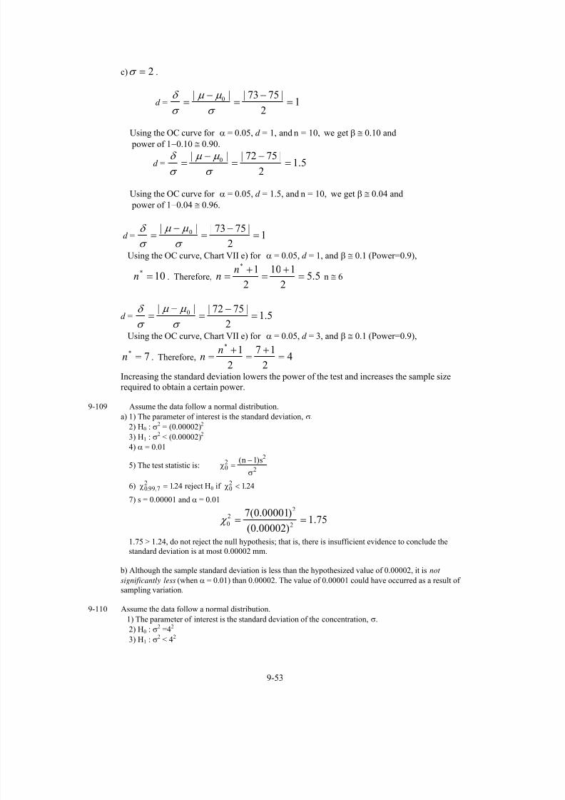
7/12/2019 Solution Manual Stats
http://slidepdf.com/reader/full/solution-manual-stats 297/588
9-53
c) 2=σ .
d = 12
|7573||| 0 =−
=−
=σ
μ μ
σ
δ
Using the OC curve for α = 0.05, d = 1, and n = 10, we get β ≅ 0.10 and
power of 1−0.10 ≅ 0.90.
d = 5.12
|7572||| 0 =−
=−
=σ
μ μ
σ
δ
Using the OC curve for α = 0.05, d = 1.5, and n = 10, we get β ≅ 0.04 and
power of 1−0.04 ≅ 0.96.
d = 12
|7573||| 0 =−
=−
=σ
μ μ
σ
δ
Using the OC curve, Chart VII e) for α = 0.05, d = 1, and β ≅ 0.1 (Power=0.9),
10* =n . Therefore, 5.52
110
2
1*
=+
=+
=n
n n ≅ 6
d = 5.12
|7572||| 0 =−
=−
=σ
μ μ
σ
δ
Using the OC curve, Chart VII e) for α = 0.05, d = 3, and β ≅ 0.1 (Power=0.9),
7* =n . Therefore, 42
17
2
1*
=+
=+
=n
n
Increasing the standard deviation lowers the power of the test and increases the sample size
required to obtain a certain power.
9-109 Assume the data follow a normal distribution.
a) 1) The parameter of interest is the standard deviation, σ.
2) H0 : σ2 = (0.00002)2
3) H1 : σ2< (0.00002)
2
4) α = 0.01
5) The test statistic is: χσ
02
2
2
1=
−( )n s
6) χ0 99 72 124. , .= reject H0 if χ0
2 124< .
7) s = 0.00001 and α = 0.01
75.1)00002.0(
)00001.0(72
22
0 == χ
1.75 > 1.24, do not reject the null hypothesis; that is, there is insufficient evidence to conclude the
standard deviation is at most 0.00002 mm.
b) Although the sample standard deviation is less than the hypothesized value of 0.00002, it is not
significantly less (when α = 0.01) than 0.00002. The value of 0.00001 could have occurred as a result of
sampling variation.
9-110 Assume the data follow a normal distribution.
1) The parameter of interest is the standard deviation of the concentration, σ.
2) H0 : σ2 =42
3) H1 : σ2 < 42

7/12/2019 Solution Manual Stats
http://slidepdf.com/reader/full/solution-manual-stats 298/588
9-54
4) not given
5) The test statistic is: χσ
02
2
2
1=
−( )n s
6) will be determined based on the P-value
7) s = 0.004 and n = 10
000009.0)4(
)004.0(92
22
0 == χ
P-value = ( );00009.02 < χ P .0≅− valueP
The P-value is approximately 0, therefore we reject the null hypothesis and conclude that the standard
deviation of the concentration is less than 4 grams per liter.
9-111 Create a table for the number of nonconforming coil springs (value) and the observed number of times the
number appeared. One possible table is:
Value 0 1 2 3 4 5 6 7 8 9 10 11 12 13 14 15 16 17 18 19
Obs 0 0 0 1 4 3 4 6 4 3 0 3 3 2 1 1 0 2 1 2
The value of p must be estimated. Let the estimate be denoted by psample
sample mean 9.32540
)2(19)0(2)0(1)0(0=
++++=
1865.050
325.9ˆ ===
n
meansample psample
Value Observed Expected
0 0 0.00165
1 0 0.01889
2 0 0.10608
3 1 0.38911
4 4 1.04816
5 3 2.21073 6 4 3.80118
7 6 5.47765
8 4 6.74985
9 3 7.22141
10 0 6.78777
11 3 5.65869
12 3 4.21619
13 2 2.82541
14 1 1.71190
15 1 0.94191
16 0 0.47237
17 2 0.21659
18 1 0.09103 19 2 0.03515
Since several of the expected values are less than 3, some cells must be combined resulting in the
following table:
Value Observed Expected
0-5 8 3.77462
6 4 3.80118
7 6 5.47765
8 4 6.74985

7/12/2019 Solution Manual Stats
http://slidepdf.com/reader/full/solution-manual-stats 299/588
9-55
9 3 7.22141
10 0 6.78777
11 3 5.65869
12 3 4.21619
≥13 9 6.29436
The degrees of freedom are k − p − 1 = 9 − 1 − 1 = 7
a) 1) The variable of interest is the form of the distribution for the number of nonconforming coil springs.
2) H0: The form of the distribution is binomial
3) H1: The form of the distribution is not binomial
4) α = 0.05
5) The test statistic is
( )χ0
22
1
=−
=∑
O E
E
i i
ii
k
6) Reject H0 if χ χ02
0 0 5 72 1407> =. , .
7)
χ02
2 2
377462
4 38 011
38011
9 6 29436
6 29436= +
−
+ +
−
=
(8 - 3.77462)
17.929
2
.
( . . )
.
( . )
.
8) Since 17.929 > 14.07 reject H0. We are able to conclude the distribution of nonconforming springs is
not binomial at α = 0.05.
b) P-value = 0.0123 (from Minitab)
9-112 Create a table for the number of errors in a string of 1000 bits (value) and the observed number of times the
number appeared. One possible table is:
Value 0 1 2 3 4 5
Obs 3 7 4 5 1 0
The value of p must be estimated. Let the estimate be denoted by psample
sample mean 7.1
20
)0(5)1(4)5(3)4(2)7(1)3(0=
+++++=
0017.01000
7.1ˆ ===
n
meansample psample
Value 0 1 2 3 4 5
Observed 3 7 4 5 1 0
Expected 3.64839 6.21282 5.28460 2.99371 1.27067 0.43103
Since several of the expected values are less than 3, some cells must be combined resulting in the
following table:
Value 0 1 2 ≥3
Observed 3 7 4 6
Expected 3.64839 6.21282 5.28460 4.69541
The degrees of freedom are k − p − 1 = 4 − 1 − 1 = 2
a) 1) The variable of interest is the form of the distribution for the number of errors in a string of 1000 bits.
2) H0: The form of the distribution is binomial
3) H1: The form of the distribution is not binomial
4) α = 0.05
5) The test statistic is
( )∑
=
−=
k
i i
ii
E
E O
1
2
2
0 χ

7/12/2019 Solution Manual Stats
http://slidepdf.com/reader/full/solution-manual-stats 300/588
9-56
6) Reject H0 if χ χ02
0 0 5 22 5 99> =. , .
7)
( ) ( )0.88971
69541.4
69541.46
64839.3
64839.3322
2
0 =−
++−
= χ
8) Since 0.88971 < 9.49 do not reject H0. We are unable to reject the null hypothesis that the distribution
of the number of errors is binomial at α = 0.05. b) P-value = 0.6409 (found using Minitab)
9-113 Divide the real line under a standard normal distribution into eight intervals with equal
probability. These intervals are [0,0.32), [0.32, 0.675), [0.675, 1.15), [1.15, ∞) and their negative
counterparts. The probability for each interval is p = 1/8 = 0.125 so the expected cell frequencies
are E = np = (100) (0.125) = 12.5. The table of ranges and their corresponding frequencies is
completed as follows.
Interval Obs. Frequency. Exp. Frequency.
x ≤ 5332.5 1 12.5
5332.5< x ≤ 5357.5 4 12.5
5357.5< x ≤ 5382.5 7 12.5
5382.5< x ≤ 5407.5 24 12.55407.5< x ≤ 5432.5 30 12.5
5432.5< x ≤ 5457.5 20 12.5
5457.5< x ≤ 5482.5 15 12.5
x ≥ 5482.5 5 12.5
The test statistic is:
36.635.12
)5.125(
5.12
12.5)-(15
5.12
)5.124(
5.12
12.5)-(1
22222
0 =−
+++−
+= χ
and we would reject if this value exceeds 07.115,05.02 = χ . Because
2
5,05.0
2 χ χ >o , reject the
hypothesis that the data are normally distributed
9-114 a) In order to use t statistics in hypothesis testing, we need to assume that the underlying distribution
is normal.
1) The parameter of interest is the true mean concentration of suspended solids, μ.
2) H0 : μ = 50
3) H1 : μ < 50
4) α = 0.05
5) Since n>>30 we can use the normal distribution
z0 =
ns
x
/
μ −
6) Reject H0 if z0 <- zα where z0.05 =1.657) x = 59.87 s = 12.50 n = 60
z0 = 12.660/50.12
5087.59=
−
8) Since 6.12>-1.65, do not reject the null hypothesis and conclude there is insufficient evidence to indicate that
the true mean concentration of suspended solids is less than 50 ppm at α = 0.05.
b) The P-value = 1)12.6( ≅Φ .
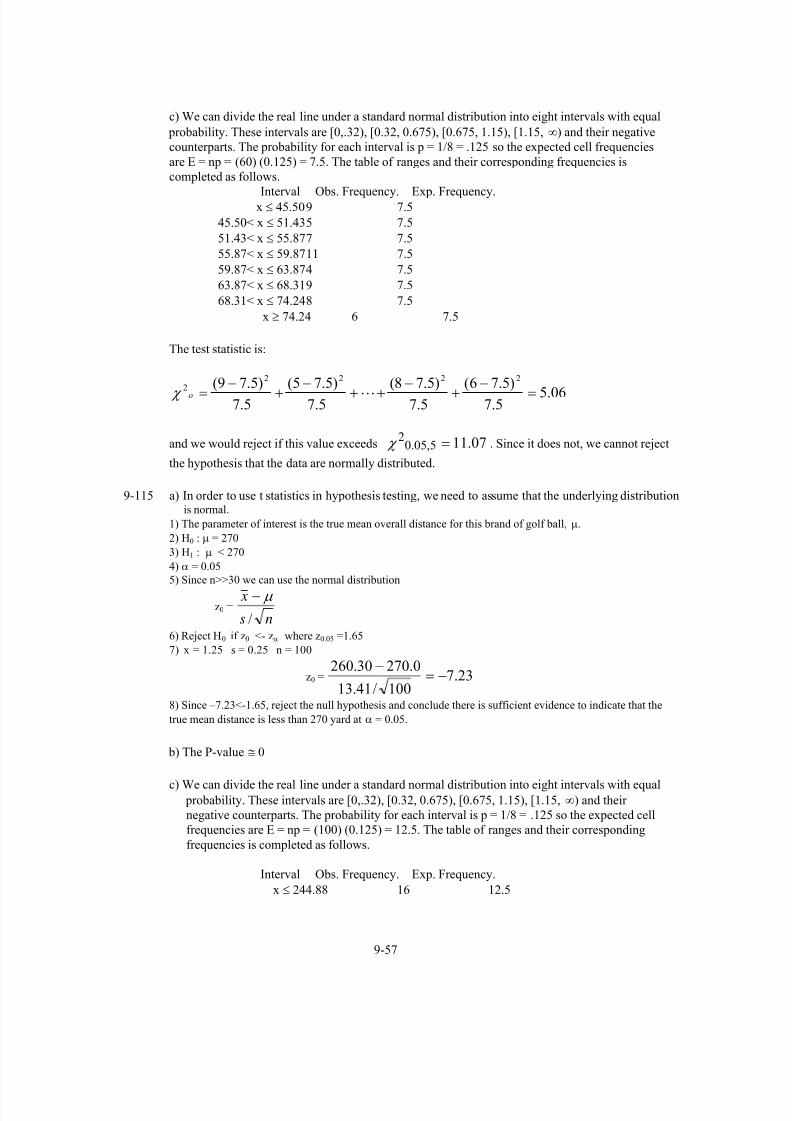
7/12/2019 Solution Manual Stats
http://slidepdf.com/reader/full/solution-manual-stats 301/588
9-57
c) We can divide the real line under a standard normal distribution into eight intervals with equal
probability. These intervals are [0,.32), [0.32, 0.675), [0.675, 1.15), [1.15, ∞) and their negative
counterparts. The probability for each interval is p = 1/8 = .125 so the expected cell frequencies
are E = np = (60) (0.125) = 7.5. The table of ranges and their corresponding frequencies is
completed as follows.
Interval Obs. Frequency. Exp. Frequency.x ≤ 45.50 9 7.5
45.50< x ≤ 51.43 5 7.5
51.43< x ≤ 55.87 7 7.5
55.87< x ≤ 59.87 11 7.5
59.87< x ≤ 63.87 4 7.5
63.87< x ≤ 68.31 9 7.5
68.31< x ≤ 74.24 8 7.5
x ≥ 74.24 6 7.5
The test statistic is:
06.55.7
)5.76(5.7
)5.78(5.7
)5.75(5.7
)5.79(2222
2 =−+−++−+−= o χ
and we would reject if this value exceeds 07.115,05.02 = χ . Since it does not, we cannot reject
the hypothesis that the data are normally distributed.
9-115 a) In order to use t statistics in hypothesis testing, we need to assume that the underlying distributionis normal.
1) The parameter of interest is the true mean overall distance for this brand of golf ball, μ.
2) H0 : μ = 270
3) H1 : μ < 270
4) α = 0.05
5) Since n>>30 we can use the normal distribution
z0 =
ns
x
/
μ −
6) Reject H0 if z0 <- zα where z0.05 =1.65
7) x = 1.25 s = 0.25 n = 100
z0 = 23.7100/41.13
0.27030.260−=
−
8) Since –7.23<-1.65, reject the null hypothesis and conclude there is sufficient evidence to indicate that the
true mean distance is less than 270 yard at α = 0.05.
b) The P-value ≅ 0
c) We can divide the real line under a standard normal distribution into eight intervals with equal
probability. These intervals are [0,.32), [0.32, 0.675), [0.675, 1.15), [1.15, ∞) and their
negative counterparts. The probability for each interval is p = 1/8 = .125 so the expected cell
frequencies are E = np = (100) (0.125) = 12.5. The table of ranges and their corresponding
frequencies is completed as follows.
Interval Obs. Frequency. Exp. Frequency.
x ≤ 244.88 16 12.5

7/12/2019 Solution Manual Stats
http://slidepdf.com/reader/full/solution-manual-stats 302/588
9-58
244.88< x ≤ 251.25 6 12.5
251.25< x ≤ 256.01 17 12.5
256.01< x ≤ 260.30 9 12.5
260.30< x ≤ 264.59 13 12.5
264.59< x ≤ 269.35 8 12.5
269.35< x ≤ 275.72 19 12.5
x ≥ 275.72 12 12.5
The test statistic is:
125.12
)5.1212(
5.12
)5.1219(
5.12
)5.126(
5.12
)5.1216( 22222 =
−+
−++
−+
−= o χ
and we would reject if this value exceeds 07.115,05.02 = χ . Because it does, we can reject the
hypothesis that the data are normally distributed.
9-116 a) In order to use t statistics in hypothesis testing, we need to assume that the underlying distributionis normal.
1) The parameter of interest is the true mean coefficient of restitution, μ.2) H0 : μ = 0.635
3) H1 : μ > 0.635
4) α = 0.01
5) Since n>30 we can use the normal distribution
z0 =
ns
x
/
μ −
6) Reject H0 if z0 > zα where z0.05 =2.33
7) x = 0.624 s = 0.0131 n = 40
z0 = 31.540/0131.0
635.0624.0−=
−
8) Since –5.31< 2.33, do not reject the null hypothesis and conclude there is insufficient evidence to indicate
that the true mean coefficient of restitution is greater than 0.635 at α = 0.01.
b) The P-value )31.5(Φ ≅ 1
c.) If the lower bound of the CI was above the value 0.635 then we could conclude that the mean coefficient
of restitution was greater than 0.635.
9-117 a) In order to use t statistics in hypothesis testing, we need to assume that the underlying distributionis normal. Use the t-test to test the hypothesis that the true mean is 2.5 mg/L.
1) State the parameter of interest: The parameter of interest is the true mean dissolved oxygen level, μ.
2) State the null hypothesis H0 : μ = 2.5
3) State the alternative hypothesis H1 : μ ≠ 2.5
4) Give the significance level α = 0.055) Give the statistic
t0 =
ns
x
/
μ −
6) Reject H0 if |t0 | <tα/2,n-1
7) Sample statistic x = 3.265 s =2.127 n = 20
and calculate the t-statistic t0 =
ns
x
/
μ −

7/12/2019 Solution Manual Stats
http://slidepdf.com/reader/full/solution-manual-stats 303/588
9-59
8) Draw your conclusion and find the P-value.
b) Assume the data are normally distributed.1) The parameter of interest is the true mean dissolved oxygen level, μ.
2) H0 : μ = 2.5
3) H1 : μ ≠ 2.5
4) α = 0.055)Test statistic
t0 =
ns
x
/
μ −
6) Reject H0 if |t0 | >tα/2,n-1 where tα/2,n-1= t0.025,19b =2.093
7) x = 3.265 s =2.127 n = 20
t0 = 608.120/127.2
5.2265.3=
−
8) Since 1.608 < 2.093, do not reject the null hypotheses and conclude that the true mean is not significantly
different from 2.5 mg/L
c) The value of 1.608 is found between the columns of 0.05 and 0.1 of table V. Therefore the P-value is between 0.1 and 0.2. Minitab provides a value of 0.124
d) The confidence interval found in exercise 8-81 b. agrees with the hypothesis test above. The value of 2.5 is
within the 95% confidence limits. The confidence interval shows that the interval is quite wide due to the large
sample standard deviation value.
260.4270.2
20
127.2093.2265.3
20
127.2093.2265.3
19,025.019,025.0
≤≤
+≤≤−
+≤≤−
μ
μ
μ n
st x
n
st x
9-118 a)
1) The parameter of interest is the true mean sugar concentration, μ.
2) H0 : μ = 11.5
3) H1 : μ ≠ 11.5
4) α = 0.05
5)ns
xt
/0
μ −=
6) Reject H0 if |t0| > tα/2,n-1 where tα/2,n-1 = 2.093
7) 47.11= x , s = 0.022 n=20
10.620/022.0
5.1147.11
0
−=−
=t
8) Since 6.10 > 2.093, reject the null hypothesis and conclude that there is sufficient evidence that
the true mean sugar concentration is different from 11.5 at α = 0.05.
From table V the t0 value in absolute value is greater than the value corresponding to 0.0005 with
19 degrees of freedom. Therefore 2*0.0005 = 0.001>P-value

7/12/2019 Solution Manual Stats
http://slidepdf.com/reader/full/solution-manual-stats 304/588
9-60
b) d = 54.4022.0
|5.114.11||| 0 =−
=−
=σ
μ μ
σ
δ
Using the OC curve, Chart VII e) for α = 0.05, d = 4.54, and 20=n we find
β ≅ 0 and the Power ≅ 1.
c) d = 27.2022.0
|5.1145.11||| 0 =−
=−
=σ
μ μ
σ
δ
Using the OC curve, Chart VII e) for α = 0.05, d = 2.27, and 1-β>0.9 (β<0.1),
We find that n should be at least 5.
d) 95% two sided confidence interval
⎟ ⎠
⎞⎜⎝
⎛ +≤≤⎟
⎠
⎞⎜⎝
⎛ −
n
st x
n
st x 19,025.019,025.0 μ
48.1146.11
20022.0093.247.11
20022.0093.247.11
≤≤
⎟ ⎠ ⎞⎜⎝ ⎛ +≤≤⎟ ⎠ ⎞⎜⎝ ⎛ −
μ
μ
We can conclude that the mean sugar concentration content is not equal to 11.5 because that value
is not inside the confidence interval.
e) The normality plot below indicates that the normality assumption is reasonable.
Sugar Concentr at ion
P e r c e n
t
11.5211.5011.4811.4611.4411.4211.40
99
95
90
80
70
6050
40
30
20
10
5
1
Probabilit y Plot of Sugar Concentrati onNormal
9-119 a)
1) The parameter of interest is the true mean body weight, μ.
2) H0 : μ = 300
3) H1 : μ ≠ 300
4) α = 0.05
5)ns
xt
/0
μ −=
6) Reject H0 if |t0| > tα/2,n-1 where tα/2,n-1 = 2.056
7) 50.325= x , s = 198.79 n=27

7/12/2019 Solution Manual Stats
http://slidepdf.com/reader/full/solution-manual-stats 305/588
9-61
667.027/79.198
3005.3250 =
−=t
8) Since 0.667< 2.056, we fail to reject the null hypothesis and conclude that there is not sufficient
evidence that the true mean body weight is different from 300 at α = 0.05.
b) From table V the t0 value is found between the values of 0.25 and 0.4 with 26 degrees of
freedom, so 0.5 < P-value < 0.8 The smallest level of significance at which we would willing to
reject the null hypothesis is the P-value
c) 95% two sided confidence interval
⎟ ⎠
⎞⎜⎝
⎛ +≤≤⎟
⎠
⎞⎜⎝
⎛ −
n
st x
n
st x 19,025.019,025.0 μ
16.40484.246
27
79.198056.25.325
27
79.198056.25.325
≤≤
⎟⎟ ⎠
⎞⎜⎜⎝
⎛ −≤≤⎟⎟
⎠
⎞⎜⎜⎝
⎛ −
μ
μ
There is not enough evidence to conclude that the mean body weight differs from 300 because 300
is within the 95% confidence interval.
9-120
a)
1) The parameter of interest is the true mean percent protein, μ.
2) H0 : μ = 80
3) H1 : μ > 80
4) α = 0.05
5) t0 =ns
x
/
μ −
6) Reject H0 if t0 > tα,n-1 where t0.05,15 = 1.753
7) x = 80.68 s = 7.38 n = 16
t0 = 37.016/38.7
8068.80=
−
8) Since 0.37 < 1.753, do not reject the null hypothesis and conclude that there is not
sufficient evidence to indicate that the true mean percent protein is greater than 80 at α =
0.05.
b) From the normal probability plot, the normality assumption seems reasonable:

7/12/2019 Solution Manual Stats
http://slidepdf.com/reader/full/solution-manual-stats 306/588
9-62
percent protein
P e r c e n t
10090807060
99
95
90
80
70
60
50
40
30
20
10
5
1
Probabili ty Plot of percent proteinNormal
c) The 0.25 < P-value < 0.4, based on Table V.
9-121
a) In order to use the χ2 statistic in hypothesis testing and confidence interval construction, we
need to assume that the underlying distribution is normal.
1) The parameter of interest is the true variance of tissue assay, σ2.
2) H0 : σ2 = 0.6
3) H1 : σ2 ≠ 0.6
4) α = 0.01
5) χ02 =
( )n s− 1 2
2σ
6) Reject H0 if χ χ α02
1 2 12< − −/ ,n where =2
11,995.0 χ 2.60 or 2
1,2/
2
0 −> nα χ χ where
=2
11,005.0 χ 26.76
7) n = 12, s = 0.758
χ02 = 53.10
6.0
)758.0(11)1( 2
2
2
==−σ
sn
8) Since 2.6< 53.10 <26.76 we fail to reject H0 and conclude there is not sufficient evidence to
indicate the true variance of tissue assay is significantly different from 0.6 at α = 0.01.
b) P-value: 0.1<p-value/2<0.5 then 0.2<p-value<1
c) 99% confidence interval for σ, first find the confidence interval for σ2
For α = 0.05 and n = 12, =2
11,995.0 χ 2.60 and =2
11,005.0 χ 26.76
60.2
)758.0(11
76.26
)758.0(11 22
2
≤≤σ
0.236≤ σ2 ≤ 2.43
Because 0.6 falls within the 99% confidence bounds we would conclude that we don’t have
enough evidence to conclude that the population variance is different from 0.6
9-122

7/12/2019 Solution Manual Stats
http://slidepdf.com/reader/full/solution-manual-stats 307/588
9-63
a) In order to use the χ2 statistic in hypothesis testing and confidence interval construction, we
need to assume that the underlying distribution is normal.
1) The parameter of interest is the true variance of the ratio between the numbers of
symmetrical and total synapses, σ2.
2) H0 : σ2= 0.02
3) H1 : σ2 ≠ 0.02
4) α = 0.05
5) χ02 =
( )n s− 1 2
2σ
6) Reject H0 if χ χ α02
1 2 12< − −/ ,n where 79.162
30,975.0 = χ or 2
1,2/
2
0 −> nα χ χ where
=2
30,025.0 χ 46.98
7) n = 31, s = 0.198
χ02 = 81.58
02.0
)198.0(30)1( 2
2
2
==−σ
sn
8) Because 58.81 > 46.98 reject H0 and conclude that the true variance of the ratio between the
numbers of symmetrical and total synapses is significantly different from 0.02 at α = 0.05.
b) P-value/2<0.005 so that P-value<0.01
9-123 a)
1) The parameter of interest is the true mean of cut-on wave length, μ.
2) H0 : μ = 6.5
3) H1 : μ ≠ 6.5
4) A value for α is not given. We assume that α = 0.05.
5)ns
xt
/0
μ −=
6) Reject H0 if |t0| > tα/2,n-1 where tα/2,n-1 = 2.228
7) 55.6= x , s = 0.35 n=11
47.011/35.0
5.655.60 =
−=t
8) Since 0.47< 2.228, we fail to reject the null hypothesis and conclude that there is not
sufficient
evidence that the true mean of cut-on wave length is different from 6.5 at α = 0.05.
b) From table V the t0 value is found between the values of 0.25 and 0.4 with 10 degrees of
freedom, so 0.5<P-value<0.8
c) d = 71.035.0
|5.625.6||| 0
=−
=−
= σ
μ μ
σ
δ
Using the OC curve, Chart VII e) for α = 0.05, d = 0.71, and 1-β > 0.95 (β<0.05),
We find that n should be at least 30.
d) d = 28.135.0
|5.695.6||| 0 =−
=−
=σ
μ μ
σ
δ
Using the OC curve, Chart VII e) for α = 0.05, n=11, d = 1.28, we find β≈0.1
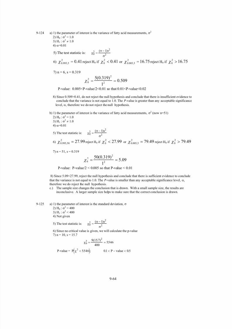
7/12/2019 Solution Manual Stats
http://slidepdf.com/reader/full/solution-manual-stats 308/588
9-64
9-124 a) 1) the parameter of interest is the variance of fatty acid measurements, σ2
2) H0 : σ2 = 1.0
3) H1 : σ2 ≠ 1.0
4) α=0.01
5) The test statistic is: χ
σ
02
2
2
1=
−( )n s
6) 41.02
5,995.0 = χ reject H0 if 41.02
0 < χ or 75.162
5,005.0 = χ reject H0 if 75.162
0 > χ
7) n = 6, s = 0.319
509.01
)319.0(52
22
0 == χ
P-value: 0.005<P-value/2<0.01 so that 0.01<P-value<0.02
8) Since 0.509>0.41, do not reject the null hypothesis and conclude that there is insufficient evidence to
conclude that the variance is not equal to 1.0. The P-value is greater than any acceptable significance
level, α, therefore we do not reject the null hypothesis.
b) 1) the parameter of interest is the variance of fatty acid measurements, σ2
(now n=51)2) H0 : σ2 = 1.0
3) H1 : σ2 ≠ 1.0
4) α=0.01
5) The test statistic is: χσ
02
2
2
1=
−( )n s
6) 99.272
50,995.0 = χ reject H0 if 99.272
0 < χ or 49.792
5,005.0 = χ reject H0 if 49.792
0 > χ
7) n = 51, s = 0.319
09.51
)319.0(502
22
0 == χ
P-value: P-value/2 < 0.005 so that P-value < 0.01
8) Since 5.09<27.99, reject the null hypothesis and conclude that there is sufficient evidence to conclude
that the variance is not equal to 1.0. The P-value is smaller than any acceptable significance level, α,
therefore we do reject the null hypothesis.
c.) The sample size changes the conclusion that is drawn. With a small sample size, the results are
inconclusive. A larger sample size helps to make sure that the correct conclusion is drawn.
9-125 a) 1) the parameter of interest is the standard deviation, σ
2) H0 : σ2 = 400
3) H1 : σ2 < 400
4) Not given
5) The test statistic is: χ
σ02
2
2
1=
−( )n s
6) Since no critical value is given, we will calculate the p-value
7) n = 10, s = 15.7
χ02
29 15 7
4005546= =
( . ).
P-value = ( )P χ2 5546< . ; 01 05. .< − <P value

7/12/2019 Solution Manual Stats
http://slidepdf.com/reader/full/solution-manual-stats 309/588
8) The P-value is greater than any acceptable significance level α. Therefore, we do not reject the null
hypothesis. There is insufficient evidence to support the claim that the standard deviation is less than
20 microamps.
b) 7) n = 51, s = 20
χ0
2250 157
400 3081= =
( . )
.
P-value = ( )P χ2 3081< . ; 0 01 0 025. .< − <P value
8) The P-value is less than 0.05, therefore we reject the null hypothesis and conclude that the standard
deviation is significantly less than 20 microamps.
c) Increasing the sample size increases the test statistic χ02 and therefore decreases the P-value, providing
more evidence against the null hypothesis.
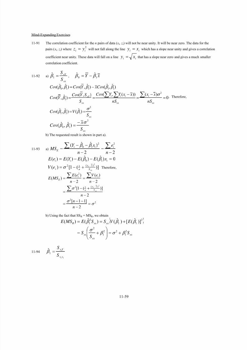
7/12/2019 Solution Manual Stats
http://slidepdf.com/reader/full/solution-manual-stats 310/588
11-59
Mind-Expanding Exercises
11-91 The correlation coefficient for the n pairs of data ( xi , zi) will not be near unity. It will be near zero. The data for the
pairs ( xi , zi) where2
ii y z = will not fall along the line ii x y = which has a slope near unity and gives a correlation
coefficient near unity. These data will fall on a line ii x y = that has a slope near zero and gives a much smaller
correlation coefficient.
11-92 a)
xx
xY
S
S=1
ˆ β , xY 10ˆˆ β β −=
xx
xx
i
xx
iii
xx
xY
SV Cov
nS
x x
nS
x xY Y Cov
S
SY CovY Cov
Cov xY CovCov
2
111
2
1
11110
)ˆ()ˆ,ˆ(
0)())(,(),(
)ˆ,(
)ˆ,ˆ()ˆ,()ˆ,ˆ(
σ β β β
σ β
β β β β β
==
=−
=−
==
−=
∑∑∑ . Therefore,
xxS
xCov
2
10 )ˆ,ˆ(σ
β β −=
b) The requested result is shown in part a).
11-93 a)22
)ˆˆ( 22
10
−=
−
−−= ∑∑
n
e
n
xY MS
iii
E
β β
0)ˆ()ˆ()()( 10 =−−= iii x E E Y E e E β β
)](1[)(2)(12
xx
i
S
x x
nieV −+−=σ Therefore,
22
)(12
2
2
]11[
2
)](1[
2
)(
2
)()(
2
σ σ
σ
=−
−−=
−
+−=
−=
−=
∑
∑∑
−
n
n
n
n
eV
n
e E MS E
xx
i
S
x x
n
ii
E
b) Using the fact that SSR = MSR , we obtain
xx
xx
xx
xx xx R
SS
S
E V SS E MS E
2
1
22
1
2
2
11
2
1 )]ˆ([)ˆ()ˆ()(
β σ β σ
β β β
+=⎟⎟ ⎠
⎞⎜⎜⎝
⎛ +=
+==
11-94
11
1
1ˆ
x x
Y x
S
S= β

7/12/2019 Solution Manual Stats
http://slidepdf.com/reader/full/solution-manual-stats 311/588
11-60
11
21
11
12
11
11
121
11
1
2
11
121
1
12101
1
1
)(
))(()(
)ˆ(
x x
x x
x x
n
i
x x
x x
n
i
x x
n
i
i
SS
S
x x xS
S
x x x x
S
x xY E
E
ii
iiii
β β
β β
β β β
β
+=−+
=
−++=
⎥⎦
⎤⎢⎣
⎡−
=
∑
∑∑
=
==
No, β1 is no longer unbiased.
11-95
xxSV
2
1 )ˆ(σ
β = . To minimize xxSV ),ˆ( 1 β should be maximized. Because ∑=
−=n
i
i xx x xS1
2)( , Sxx is
maximized by choosing approximately half of the observations at each end of the range of x.
From a practical perspective, this allocation assumes the linear model between Y and x holds throughout the range of x
and observing Y at only two x values prohibits verifying the linearity assumption. It is often preferable to obtain some
observations at intermediate values of x.
11-96 One might minimize a weighted some of squares ∑=
−−n
i
iii x yw1
2
10 )( β β in which a Y i with small variance
(wi large) receives greater weight in the sum of squares.
i
n
i
iii
n
i
iii
n
i
iii
n
i
iii
x x yw x yw
x yw x yw
∑∑
∑∑
==
==
−−−=−−
−−−=−−
1
10
1
2
10
1
1
10
1
2
10
0
)(2)(
)(2)(
β β β β β
∂
β β β β β
∂
Setting these derivatives to zero yields
∑∑∑
∑∑∑
=+
=+
iiiiiii
iiiii
y xw xw xw
yw xww
2
10
10
ˆˆ
ˆˆ
β β
β β
and these equations are solved as follows
( )( )( )( ) ( )22
1ˆ
∑∑∑∑∑∑
−
−=
iiiii
iiiiii
xw xww
yww y xw β
10ˆˆ β β
∑∑∑∑−=
i
ii
i
ii
w xw
w yw .
11-97 )(ˆ x xs
sr y y
x
y −+=

7/12/2019 Solution Manual Stats
http://slidepdf.com/reader/full/solution-manual-stats 312/588
11-61
x x x y
x xS
S y
x xSS
x x y yS y
xx
xy
i yy xx
i xy
1011
2
2
ˆˆˆˆ
)(
)(
)()(
β β β β +=−+=
−+=
−
−−+=
∑∑
11-98 a) i
n
i
ii
n
i
ii x x y x y ∑∑==
−−−=−−1
10
1
2
10
1
)(2)( β β β β β
∂
Upon setting the derivative to zero, we obtain
∑∑∑ =+ iiii y x x x2
10 β β
Therefore,
∑
∑
∑
∑ ∑ −=
−=
2
0
2
0
1
)(ˆ
i
ii
i
iii
x
y x
x
x y x β β β
b)
∑∑∑
∑∑ ==
⎟⎟
⎠
⎞
⎜⎜
⎝
⎛ −=
2
2
22
22
2
0
1][
)()ˆ(
ii
i
i
ii
x x
x
x
Y xV V
σ σ β β
c)∑−± 2
2ˆ1,2/1
ˆi xnt σ
α β
This confidence interval is shorter because ∑∑ −≥ 22)( x x x ii . Also, the t value based on n-1 degrees of
freedom is slightly smaller than the corresponding t value based on n-2 degrees of freedom.

7/12/2019 Solution Manual Stats
http://slidepdf.com/reader/full/solution-manual-stats 313/588
11-1
CHAPTER 11
Section 11-2
11-1 a) iii x y ε β β ++= 10
348571.2542.157 1443
2
=−= xxS
057143.5980.169714
)572(43 −=−= xyS
.
..
( . )( ) .
β
β β
1
0 157214
4314
59 057143
253485712 330
2 3298017 48 013
= =−
= −
= − = − − =
S
S
y x
xy
xx
123.22
59143.13771429.159
59.137
)057143.59(3298017.2ˆ1
=
−=
−=
=
−−==
R yy E
xy R
SSSSS
SSS β
8436112
12322
2
2.
.
n
SS MSˆ E
E ==−
==σ
b) x y 10ˆˆˆ β β +=
99.37)3.4(3298017.2012962.48ˆ =−= y
c) 39.39)7.3(3298017.2012962.48ˆ =−= y
d) 71.639.391.46ˆ =−=−= y ye
11-2 a) iii x y ε β β ++= 10
6.339918.14321520
14782
=−= xxS
445.14167.108320
)75.12)(1478( =−= xyS
32999.0))(0041617512.0(ˆ
00416.06.33991
445.141ˆ
201478
2075.12
0
1
=−=
===
β
β xx
xy
S
S
x y 00416.032999.0ˆ +=
00796.018
143275.0
2ˆ 2 ==
−==
n
SS MS E
E σ

7/12/2019 Solution Manual Stats
http://slidepdf.com/reader/full/solution-manual-stats 314/588
11-2
0
0.1
0.20.3
0.4
0.5
0.6
0.7
0.8
-50 0 50 100
x
y
b) 6836.0)85(00416.032999.0ˆ =+= y
c) 7044.0)90(00416.032999.0ˆ =+= y
d) 00416.0ˆ1 = β
11-3 a) The regression equation is Rating Pts = - 5.56 + 12.7 Yds per Att
Predictor Coef SE Coef T P
Constant -5.558 9.159 -0.61 0.549
Yds per Att 12.652 1.243 10.18 0.000
S = 5.71252 R-Sq = 78.7% R-Sq(adj) = 78.0%
Analysis of Variance
Source DF SS MS F P
Regression 1 3378.5 3378.5 103.53 0.000
Residual Error 28 913.7 32.6
Total 29 4292.2
iii x y ε β β ++= 10
106.2130
)55.219(847.1627
2
=−= xxS
037.26730
)2611)(55.219(21.19375 =−= xyS
56.530
55.219)652.12(30
2611ˆ
652.12106.21
037.267ˆ
0
1
−=⎟ ⎠
⎞⎜⎝
⎛ −=
===
β
β xx
xy
S
S
x y 652.1256.5ˆ +−=
6.3228
7.913
2ˆ 2 ==
−==
n
SS MS E
E σ

7/12/2019 Solution Manual Stats
http://slidepdf.com/reader/full/solution-manual-stats 315/588
11-3
Yds per At t
R a t i n g
P t s
98765
120
110
100
90
80
70
60
S 5.71252
R-Sq 78.7%
R-Sq(adj) 78.0%
Fitted Line PlotRating Pts = - 5.558 + 12.65 Yds per Att
b) 33.89)5.7(652.1256.5ˆ =+−= y
c) 652.12ˆ1 −=− β
d) 79.010652.12
1=×
e) 66.85)21.7(652.1256.5ˆ =+−= y
56.766.851.78
ˆ
−=−=
−= y ye
11-4 a)Regression Analysis - Linear model: Y = a+bX
Dependent variable: SalePrice Independent variable: Taxes
--------------------------------------------------------------------------------
Standard T Prob.
Parameter Estimate Error Value Level
Intercept 13.3202 2.57172 5.17948 .00003
Slope 3.32437 0.390276 8.518 .00000
--------------------------------------------------------------------------------
Analysis of Variance
Source Sum of Squares Df Mean Square F-Ratio Prob. Level
Model 636.15569 1 636.15569 72.5563 .00000
Residual 192.89056 22 8.76775
--------------------------------------------------------------------------------
Total (Corr.) 829.04625 23
Correlation Coefficient = 0.875976 R-squared = 76.73 percent
Stnd. Error of Est. = 2.96104
76775.8ˆ 2 =σ
If the calculations were to be done by hand, use Equations (11-7) and (11-8). x y 32437.33202.13ˆ +=
b) 253.38)5.7(32437.33202.13ˆ =+= y
c) 9273.32)8980.5(32437.33202.13ˆ =+= y
0273.29273.329.30ˆ
9273.32ˆ
−=−=−=
=
y ye
y

7/12/2019 Solution Manual Stats
http://slidepdf.com/reader/full/solution-manual-stats 316/588
11-4
d) All the points would lie along a 45 degree line. That is, the regression model would estimate the values exactly. At
this point, the graph of observed vs. predicted indicates that the simple linear regression model provides a reasonable
fit to the data.
25 30 35 40 45 50
Observed
25
30
35
40
45
50
P r e d i c t e d
Plot of Observed values versus predicted

7/12/2019 Solution Manual Stats
http://slidepdf.com/reader/full/solution-manual-stats 317/588
11-5
11-5 a)Regression Analysis - Linear model: Y = a+bX
Dependent variable: Usage Independent variable: Temperature
--------------------------------------------------------------------------------
Standard T Prob.
Parameter Estimate Error Value Level
Intercept -6.3355 1.66765 -3.79906 .00349
Slope 9.20836 0.0337744 272.643 .00000
--------------------------------------------------------------------------------
Analysis of Variance
Source Sum of Squares Df Mean Square F-Ratio Prob. Level
Model 280583.12 1 280583.12 74334.4 .00000
Residual 37.746089 10 3.774609
--------------------------------------------------------------------------------
Total (Corr.) 280620.87 11
Correlation Coefficient = 0.999933 R-squared = 99.99 percent
Stnd. Error of Est. = 1.94284
7746.3ˆ 2 =σ
If the calculations were to be done by hand, use Equations (11-7) and (11-8).
x y 20836.93355.6ˆ +−=
b) 124.500)55(20836.93355.6ˆ =+−= y
c) If monthly temperature increases by 1 F, y increases by 9.20836.
d) 458.426)47(20836.93355.6ˆ =+−= y
.y = 426458
618.1458.42684.424ˆ −=−=−= y ye
11-6 a)The regression equation is MPG = 39.2 - 0.0402 Engine Replacement
Predictor Coef SE Coef T P
Constant 39.156 2.006 19.52 0.000
Engine Replacement -0.040216 0.007671 -5.24 0.000
S = 3.74332 R-Sq = 59.1% R-Sq(adj) = 57.0%
Analysis of Variance
Source DF SS MS F P
Regression 1 385.18 385.18 27.49 0.000
Residual Error 19 266.24 14.01
Total 20 651.41
01.14ˆ 2 =σ
x y 0402.02.39ˆ −=
b) 17.33)150(0402.02.39ˆ =−= y
c) 2956.34ˆ = y
0044.72956.343.41ˆ =−=−= y ye

7/12/2019 Solution Manual Stats
http://slidepdf.com/reader/full/solution-manual-stats 318/588
11-6
11-7 a)
1050950850
60
50
40
x
y
Predictor Coef StDev T PConstant -16.509 9.843 -1.68 0.122x 0.06936 0.01045 6.64 0.000S = 2.706 R-Sq = 80.0% R-Sq(adj) = 78.2% Analysis of VarianceSource DF SS MS F PRegression 1 322.50 322.50 44.03 0.000Error 11 80.57 7.32Total 12 403.08
3212.7ˆ 2 =σ
x y 0693554.05093.16ˆ +−=
b) 6041.46ˆ = y 39592.1ˆ =−= y ye
c) 38.49)950(0693554.05093.16ˆ =+−= y
11-8 a)
10090807060
9
8
7
65
4
3
2
1
0
x
y
Yes, a linear regression would seem appropriate, but one or two points might be outliers.
Predictor Coef SE Coef T P
Constant -10.132 1.995 -5.08 0.000
x 0.17429 0.02383 7.31 0.000
S = 1.318 R-Sq = 74.8% R-Sq(adj) = 73.4%
Analysis of Variance
Source DF SS MS F P
Regression 1 92.934 92.934 53.50 0.000
Residual Error 18 31.266 1.737
Total 19 124.200
b) 737.1ˆ 2 =σ and x y 17429.0132.10ˆ +−=
c) 68265.4ˆ = y at x = 85

7/12/2019 Solution Manual Stats
http://slidepdf.com/reader/full/solution-manual-stats 319/588
11-7
11-9 a)
403020100
250
200
150
100
x
y
Yes, a linear regression model appears to be plausible.
Predictor Coef StDev T PConstant 234.07 13.75 17.03 0.000x -3.5086 0.4911 -7.14 0.000S = 19.96 R-Sq = 87.9% R-Sq(adj) = 86.2% Analysis of VarianceSource DF SS MS F PRegression 1 20329 20329 51.04 0.000Error 7 2788 398
Total 8 23117
b) 25.398ˆ 2 =σ and x y 50856.3071.234ˆ −=
c) 814.128)30(50856.3071.234ˆ =−= y
d) 1175.15883.156ˆ == e y
11-10 a)
1.81.61.41.21.00.80.60.40.20.0
40
30
20
10
0
x
y
Yes, a simple linear regression model seems appropriate for these data.
Predictor Coef StDev T PConstant 0.470 1.936 0.24 0.811x 20.567 2.142 9.60 0.000S = 3.716 R-Sq = 85.2% R-Sq(adj) = 84.3%
Analysis of Variance
Source DF SS MS F PRegression 1 1273.5 1273.5 92.22 0.000Error 16 220.9 13.8Total 17 1494.5

7/12/2019 Solution Manual Stats
http://slidepdf.com/reader/full/solution-manual-stats 320/588
11-8
b) 81.13ˆ 2 =σ
x y 5673.20470467.0ˆ +=
c) 038.21)1(5673.20470467.0ˆ =+= y
d) 6629.11371.10ˆ == e y
11-11 a)
2520151050
2600
2100
1600
x
y
Yes, a simple linear regression (straight-line) model seems plausible for this situation.
Predictor Coef StDev T PConstant 2625.39 45.35 57.90 0.000x -36.962 2.967 -12.46 0.000
S = 99.05 R-Sq = 89.6% R-Sq(adj) = 89.0%
Analysis of VarianceSource DF SS MS F PRegression 1 1522819 1522819 155.21 0.000Error 18 176602 9811Total 19 1699421
b) 2.9811ˆ 2 =σ
x y 962.3639.2625ˆ −=
c) 15.1886)20(962.3639.2625ˆ =−= y
d) If there were no error, the values would all lie along the 45
line. The plot indicates age is reasonable
regressor variable.
1600 2100 2600
1700
1800
1900
2000
2100
2200
2300
2400
2500
2600
y
F I T S
1

7/12/2019 Solution Manual Stats
http://slidepdf.com/reader/full/solution-manual-stats 321/588
11-9
11-12
a)The regression equation is
Porosity = 55.6 - 0.0342 Temperature
Predictor Coef SE Coef T P
Constant 55.63 32.11 1.73 0.144Temperature -0.03416 0.02569 -1.33 0.241
S = 8.79376 R-Sq = 26.1% R-Sq(adj) = 11.3%
Analysis of Variance
Source DF SS MS F P
Regression 1 136.68 136.68 1.77 0.241
Residual Error 5 386.65 77.33
Total 6 523.33
x y 03416.063.55ˆ −=
33.77ˆ 2 =σ
b) 806.7)1400(03416.063.55ˆ =−= y
c) 39.4ˆ = y 012.7=e
d)
Temperature
P o r o s i t y
15001400130012001100
30
25
20
15
10
5
0
Scatter plot of Porosity vs Temperatur e
The simple linear regression model doesn’t seem appropriate because the scatter plot doesn’t show a linear
relationship between the data.
11-13 a) The regression equation is BOD = 0.658 + 0.178 Time
Predictor Coef SE Coef T PConstant 0.6578 0.1657 3.97 0.003
Time 0.17806 0.01400 12.72 0.000
S = 0.287281 R-Sq = 94.7% R-Sq(adj) = 94.1%
Analysis of Variance
Source DF SS MS F P
Regression 1 13.344 13.344 161.69 0.000

7/12/2019 Solution Manual Stats
http://slidepdf.com/reader/full/solution-manual-stats 322/588
11-10
Residual Error 9 0.743 0.083
Total 10 14.087
x y 178.0658.0ˆ +=
083.0ˆ 2 =σ
b) 328.3)15(178.0658.0ˆ =+= y
c) 0.178(3) = 0.534
d) 726.1)6(178.0658.0ˆ =+= y
174.0726.19.1ˆ =−=−= y ye
e)
y
y - h a t
4.03.53.02.52.01.51.00.5
4.5
4.0
3.5
3.0
2.5
2.0
1.5
1.0
Scatt erplot of y-hat vs y
All the points would lie along the 45 degree line y y ˆ= . That is, the regression model would estimate the
values exactly. At this point, the graph of observed vs. predicted indicates that the simple linear regression
model provides a reasonable fit to the data.
11-14 a)The regression equation is
Deflection = 32.0 - 0.277 Stress level
Predictor Coef SE Coef T P
Constant 32.049 2.885 11.11 0.000
Stress level -0.27712 0.04361 -6.35 0.000
S = 1.05743 R-Sq = 85.2% R-Sq(adj) = 83.1%
Analysis of Variance
Source DF SS MS F P
Regression 1 45.154 45.154 40.38 0.000
Residual Error 7 7.827 1.118Total 8 52.981
118.1ˆ 2 =σ
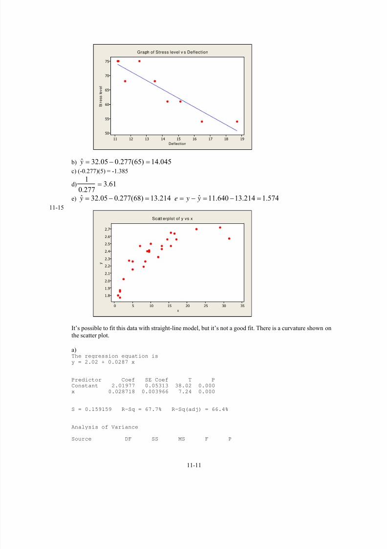
7/12/2019 Solution Manual Stats
http://slidepdf.com/reader/full/solution-manual-stats 323/588
11-11
Deflection
S t r e s s
l e v e l
191817161514131211
75
70
65
60
55
50
Graph of Stress level v s Deflection
b) 045.14)65(277.005.32ˆ =−= y
c) (-0.277)(5) = -1.385
d) 61.3277.0
1=
e) ˆ 32.05 0.277(68) 13.214 y = − = ˆ 11.640 13.214 1.574e y y= − = − =
11-15
x
y
35302520151050
2.7
2.6
2.5
2.4
2.3
2.2
2.1
2.0
1.9
1.8
Scatt erplot of y vs x
It’s possible to fit this data with straight-line model, but it’s not a good fit. There is a curvature shown on
the scatter plot.
a)The regression equation is
y = 2.02 + 0.0287 x
Predictor Coef SE Coef T PConstant 2.01977 0.05313 38.02 0.000
x 0.028718 0.003966 7.24 0.000
S = 0.159159 R-Sq = 67.7% R-Sq(adj) = 66.4%
Analysis of Variance
Source DF SS MS F P

7/12/2019 Solution Manual Stats
http://slidepdf.com/reader/full/solution-manual-stats 324/588
11-12
Regression 1 1.3280 1.3280 52.42 0.000
Residual Error 25 0.6333 0.0253
Total 26 1.9613
x y 0287.002.2ˆ +=
0253.0ˆ 2 =σ
b) 3357.2)11(0287.002.2ˆ =+= y
c)
y-hat
y
2.92.82.72.62.52.42.32.22.12.0
2.7
2.6
2.5
2.4
2.3
2.2
2.1
2.0
1.9
1.8
Scatterpl ot of y vs y-hat
If the relationship between length and age was deterministic, the points would fall on the 45 degree
line y y ˆ= . Because the points in this plot vary substantially from this line, it appears that age is not a
reasonable choice for the regressor variable in this model.
11-16 a) )32(0041612.03299892.0ˆ5
9 ++= x y
x y
x y
0074902.04631476.0ˆ
1331584.00074902.03299892.0ˆ
+=++=
b) 00749.0ˆ1 = β
11-17 Let x = engine displacement (cm3) and xold = engine displacement (in3)
a) The old regression equation is y = 39.2 - 0.0402xold
Because 1 in3 = 16.387 cm3, the new regression equation is
x x y 0025.02.39)387.16/(0402.02.39ˆ −=−=
b) 0025.0ˆ1 −= β
11-18 y x x y x =+−=+ 1110 ˆ)ˆ(ˆˆ β β β β
11-19 a) The slopes of both regression models will be the same, but the intercept will be shifted.
b) x y 9618.3641.2132ˆ −=
9618.36ˆ
39.2625ˆ
1
0
−=
=
β
β vs.
9618.36ˆ
41.2132ˆ
1
0
−=
=∗
∗
β
β

7/12/2019 Solution Manual Stats
http://slidepdf.com/reader/full/solution-manual-stats 325/588
11-13
11-20 a) The least squares estimate minimizes ∑ − 2)( ii x y β . Upon setting the derivative equal to zero, we obtain
0][2)()(22 =+−=−− ∑∑∑ iiiiii x x y x x y β β
Therefore,
∑∑=
2ˆ
i
ii
x
x y β .
b) x y 031461.21ˆ = . The model seems very appropriate—an even better fit.
0
5
10
15
20
25
30
35
40
45
0 0.2 0.4 0.6 0.8 1 1.2 1.4 1.6 1.8 2
watershed
c h l o r i d e

7/12/2019 Solution Manual Stats
http://slidepdf.com/reader/full/solution-manual-stats 326/588
11-14
Section 11-4
11-21 a) 1) The parameter of interest is the regressor variable coefficient, β1
2) H0 1 0:β =
3) H1 1 0:β ≠
4) α = 0.05
5) The test statistic is
)2/(
1/0 −
==nSS
SS
MS
MS f
E
R
E
R
6) Reject H0 if f 0 > f α,1,12 where f 0.05,1,12 = 4.75
7) Using results from Exercise 11-1
123.22
59143.13771429.159
59.137
)057143.59(3298017.2ˆ1
=
−=
−=
=
−−==
R yy E
xy R
SSSSS
SSS β
63.7412/123.22
59.1370 == f
8) Since 74.63 > 4.75 reject H 0 and conclude that compressive strength is significant in predicting intrinsic
permeability of concrete at α = 0.05. We can therefore conclude that the model specifies a useful linear
relationship between these two variables.
P value− ≅ 0 000002.
b) 8436112
12322
2
2 ..
n
SS MSˆ E
E ==−
==σ and 2696.03486.25
8436.1ˆ)ˆ(
2
1 === xxS
seσ
β
c) 9043.03486.25
0714.3
14
18436.1
1ˆ)ˆ(
222
0 =⎥
⎦
⎤⎢
⎣
⎡+=⎥
⎦
⎤⎢
⎣
⎡+=
xx
S
x
nse σ β
11-22 a) 1) The parameter of interest is the regressor variable coefficient, β1.
2) H0 1 0:β =
3) H1 1 0:β ≠
4) α = 0.05
5) The test statistic is
)n /(SS
/ SS
MS
MS f
E
R
E
R
2
10 −
==
6) Reject H0 if f 0 > f α,1,18 where f 0.05,1,18 = 4.414
7) Using the results from Exercise 11-2
SS S
SS S SS
R xy
E yy R
= =
== −
= − −
=
( . )( . )
.
( . ) .
.
.
β1
127520
0 0041612 141445
05886
886 05886
0143275
2
9573181432750
588600 .
/ .
. f ==
8) Since 73.95 > 4.414, reject H 0 and conclude the model specifies a useful relationship at α = 0.05.
P value− ≅ 0 000001.

7/12/2019 Solution Manual Stats
http://slidepdf.com/reader/full/solution-manual-stats 327/588
11-15
b)4
2
1 108391.46.33991
00796.ˆ)ˆ( −=== x
Sse
xx
σ β
04091.06.33991
9.73
20
100796.
1ˆ)ˆ(
22
0=⎥
⎦
⎤⎢⎣
⎡+=⎥
⎦
⎤⎢⎣
⎡+=
xxS
x
nse σ β
11-23 a)The regression equation is
Rating Pts = - 5.558 + 12.65 Yds per Att
S = 5.71252 R-Sq = 78.7% R-Sq(adj) = 78.0%
Analysis of Variance
Source DF SS MS F P
Regression 1 3378.53 3378.53 103.53 0.000
Error 28 913.72 32.63
Total 29 4292.25
Refer to ANOVA
01.0
0:
0:
11
10
=
≠=
α
β
β
H
H
Because p-value = 0.000 < α = 0.01, reject H0. We can conclude that there is a linear relationship between
these two variables.
b) 63.32ˆ 2 =σ
243.1106.21
63.32ˆ)ˆ(
2
1 === xxS
seσ
β
159.9106.21
318.7
30
163.32
1ˆ)ˆ(
222
0=⎥
⎦
⎤⎢⎣
⎡+=⎥
⎦
⎤⎢⎣
⎡+=
xxS
x
nse σ β
c) 1)The parameter of interest is the regressor variable coefficient, β1.
2) H0 1 10:β =
3) H1 1 10:β ≠
4) α = 0.01
5) The test statistic is)ˆ(
ˆ
1
0,11
0 β
β β
set
−=
6) Reject H0 if t0 < −tα/2,n-2 where −t0.005,28 = −2.763 or t0 > t0.005,28 = 2.763
7) Using the results from Exercise 10-6
134.2243.1
10652.120 =
−=t
8) Because 2.134 < 2.763, fail to reject H 0 . There is not enough evidence to conclude that the slope
differs from 10 at α = 0.01.
11-24 Refer to ANOVA of Exercise 11-4
a) 1) The parameter of interest is the regressor variable coefficient, β1.
2) H0 1 0:β =

7/12/2019 Solution Manual Stats
http://slidepdf.com/reader/full/solution-manual-stats 328/588
11-16
3) H1 1 0:β ≠
4) α = 0.05, using t-test
5) The test statistic is tse
01
1
=
( )
β
β
6) Reject H0 if t0 < −tα/2,n-2 where −t0.025,22 = −2.074 or t0 > t0.025,22 = 2.074
7) Using the results from Exercise 11-5
t0
332437
0 3902768518= =
.
..
8) Since 8.518 > 2.074 reject H 0 and conclude the model is useful α = 0.05.
b) 1) The parameter of interest is the slope, β1
2) H0 1 0:β =
3) H1 1 0:β ≠
4) α = 0.05
5) The test statistic is f MS
MS
SS
SS n
R
E
R
E0
1
2= =
−
/
/ ( )
6) Reject H0 if f 0 > f α,1,22 where f 0.01,1,22 = 4.303
7) Using the results from Exercise 10-5
f 063615569 1
19289056 2272 5563= =. /
. /.
8) Since 72.5563 > 4.303, reject H 0 and conclude the model is useful at a significance α = 0.05.
The F-statistic is the square of the t-statistic. The F-test is a restricted to a two-sided test, whereas the
t-test could be used for one-sided alternative hypotheses.
c) 39027563157
767582
1 ..
.
S
ˆ )ˆ (se
xx
==σ
=β
57172563157
40496
24
176758
1 22
0 ..
..
S
x
nˆ )ˆ (se
xx
=⎥⎦
⎤⎢⎣
⎡+=⎥
⎦
⎤⎢⎣
⎡+σ=β
d) 1) The parameter of interest is the intercept, β0.
2) 000 =β: H
3) 001 ≠β: H
4) α = 0.05, using t-test
5) The test statistic is)ˆ (se
ˆ t
0
00 β
β=
6) Reject H0 if t0 < −tα/2,n-2 where −t0.025,22 = −2.074 or t0 > t0.025,22 = 2.074
7) Using the results from Exercise 11-5
179.55717.2
3201.130 ==t
8) Since 5.179 > 2.074 reject H 0 and conclude the intercept is not zero at α = 0.05.

7/12/2019 Solution Manual Stats
http://slidepdf.com/reader/full/solution-manual-stats 329/588
11-17
11-25 Refer to ANOVA for Exercise 10-65
a) 1) The parameter of interest is the regressor variable coefficient, β1.
2) H0 1 0:β =
3) H1 1 0:β ≠
4) α = 0.01
5) The test statistic is )2/(
1/0 −== nSS
SS
MS
MS
f E
R
E
R
6) Reject H0 if f 0 > f α,1,22 where f 0.01,1,10 = 10.049
7) Using the results from Exercise 10-6
4.7433410/746089.37
1/12.2805830 == f
8) Since 74334.4 > 10.049, reject H 0 and conclude the model is useful α = 0.01. P-value < 0.000001
b) se( 1β̂ ) = 0.0337744, se( 0β̂ ) = 1.66765
c) 1) The parameter of interest is the regressor variable coefficient, β1.
2) H0 1 10:β =
3) H1 1 10:β ≠
4) α = 0.01
5) The test statistic is
)ˆ(
ˆ
1
0,11
0
β
β β
set
−=
6) Reject H0 if t0 < −tα/2,n-2 where −t0.005,10 = −3.17 or t0 > t0.005,10 = 3.17
7) Using the results from Exercise 10-6
37.230338.0
1021.90 −=
−=t
8) Since −23.37 < −3.17 reject H 0 and conclude the slope is not 10 at α = 0.01. P-value ≈ 0.
d) H0: β0 = 0 H1: β0 ≠ 0
8.366765.1
03355.60 −=
−−=t
P-value < 0.005. Reject H0 and conclude that the intercept should be included in the model.
11-26 Refer to ANOVA table of Exercise 11-6
a) 010 =β: H
011 ≠β: H α = 0.01
18,1,0
18,1,01.0
0
285.8
53158.4
α f f
f
f
>/
=
=
Therefore, do not reject H0. P-value = 0.04734. Insufficient evidence to conclude that the model is a useful
relationship.
b) 016628101 .)ˆ (se =β
6139620 .)ˆ (se =β

7/12/2019 Solution Manual Stats
http://slidepdf.com/reader/full/solution-manual-stats 330/588
11-18
c) 05010 .: H −=β
05011 .: H −<β
α = 0.01
180
1801
0
5522
87803001662810
05003540
,
,.
t t
.t
..
).(.t
α−</
=
=−−−
=
Therefore, do not reject H0. P-value = 0.804251. Insufficient evidence to conclude that β1 is < -0.05.
d) 0: 00 = β H 001 ≠β: H α = 0.01
18,2/0
18,005.
0
878.2
8291.12
α t t
t
t
>
=
=
Therefore, reject H0. P-value ≅ 0
11-27 Refer to ANOVA of Exercise 11-7
a) 010 =β: H
011 ≠β: H
α = 0.05
1110
11105
0
844
027944
, ,
, ,.
f f
. f
. f
α>
=
=
Therefore, reject H0. P-value = 0.00004.
b) 010452401 .)ˆ (se =β
8434690 .)ˆ (se =β
c) 000 =β: H
001 ≠β: H
α = 0.05
1120
11025
0
2012
677181
, /
,.
t |t |
.t
.t
α−</
=
−=
Therefore, do not rejectH0. P-value = 0.12166.

7/12/2019 Solution Manual Stats
http://slidepdf.com/reader/full/solution-manual-stats 331/588
11-19
11-28 Refer to ANOVA of Exercise 11-8
a) 010 =β: H
011 ≠β: H
α = 0.05
18,1,0
18,1,05.
0
414.4
53.50
α f f
f
f
>=
=
Therefore, reject H0. P-value = 0.0000009.
b) 025661301 .)ˆ (se =β
1352620 .)ˆ (se =β
c) 000 =β: H
001 ≠β: H
α = 0.05
18,2/0
18,025.
0
||
101.2
5.079-
α t t
t
t
>=
=
Therefore, reject H0. P-value = 0.000078.
11-29 Refer to ANOVA of Exercise 11-11
a) 010 =β: H
011 ≠β: H
α = 0.01
18,1,0
18,1,01.
0
285.8
2.155
α f f
f
f
>
=
=
Therefore, reject H0. P-value < 0.00001.
b) 3468451 .)ˆ (se =β
9668120 .)ˆ (se =β
c) 3010 −=β: H
3011 −≠β: H
α = 0.01
1820
18005
0
8782
34662966812
30961836
, /
,.
t |t |.t
..
)(.t
α−>/ =
−=−−−
=
Therefore, do not reject H0. P-value = 0.0153(2) = 0.0306.
d) 000 =β: H
001 ≠β: H
α = 0.01

7/12/2019 Solution Manual Stats
http://slidepdf.com/reader/full/solution-manual-stats 332/588
11-20
8782
895757
18005
0
.t
.t
,. =
=
t t0 2 18> α / , , therefore, reject H0. P-value < 0.00001.
e) H0 0 2500:β =
250001 >β: H α = 0.01
552.2
7651.23468.45
250039.2625
18,01.
0
=
=−
=
t
t
18,0 α t t > , therefore reject H0 . P-value = 0.0064.
11-30 Refer to ANOVA of Exercise 11-10
a) 010 =β: H
011 ≠β: H
α = 0.01
16,1,0
16,1,01.
0
531.8
224.92
α f f
f
f
>
=
=
Therefore, reject H0 .
b) P-value < 0.00001
c) 1416921 .)ˆ (se =β
9359110 .)ˆ (se =β
d) 000 =β: H
001
≠β: H
α = 0.01
1620
16005
0
9212
2430
, /
,.
t t
.t
.t
α>/
=
=
Therefore, do not reject H0. There is not sufficient evidence to conclude that the intercept differs from zero. Based
on this test result, the intercept could be removed from the model.

7/12/2019 Solution Manual Stats
http://slidepdf.com/reader/full/solution-manual-stats 333/588
11-21
11-31 a) Refer to ANOVA of Exercise 11-13
01.0
0:
0:
11
10
=
≠
=
α
β
β
H
H
Because the P-value = 0.000 < α = 0.01, reject H0. There is evidence of a linear relationship between these
two variables.
b) 083.0ˆ 2 =σ
The standard errors for the parameters can be obtained from the computer output or calculated as follows.
014.091.420
083.0ˆ)ˆ(
2
1 === xxS
seσ
β
1657.091.420
09.10
11
1083.0
1ˆ)ˆ(
222
0 =⎥⎦
⎤⎢⎣
⎡+=⎥
⎦
⎤⎢⎣
⎡+=
xxS
x
nse σ β
c)1) The parameter of interest is the intercept β0.
2) 0: 00 = β H
3) 0: 01 ≠ β H
4) 01.0=α
5) The test statistic is)( 0
00
β
β
set =
6) Reject H0 if 2,2/0 −−< nt t α where 250.39,005.0 −=− t or 2,2/0 −> nt t α where 250.39,005.0 =t
7) Using the results from Exercise 11-13
97.31657.0
6578.00 ==t
8) Because t0 = 3.97 > 3.250 reject H0 and conclude the intercept is not zero at α = 0.01.
11-32 a) Refer to ANOVA of Exercise 11-14
01.0
0:
0:
11
10
=
≠
=
α
β
β
H
H
Because the P-value = 0.000 < α = 0.01, reject H0. There is evidence of a linear relationship between these
two variables.
b) Yes
c) 118.1ˆ 2 =σ
0436.0588
118.1ˆ)ˆ(
2
1 === xxS
seσ
β

7/12/2019 Solution Manual Stats
http://slidepdf.com/reader/full/solution-manual-stats 334/588
11-22
885.2588
67.65
9
1118.1
1ˆ)ˆ(
222
0 =⎥⎦
⎤⎢⎣
⎡+=⎥
⎦
⎤⎢⎣
⎡+=
xxS
x
nse σ β
11-33 a)
05.0
0:
0:
11
10
=
≠
=
α
β
β
H
H
Because the P-value = 0.310 > α = 0.05, fail to reject H0. There is not sufficient evidence of a linear
relationship between these two variables.
The regression equation is
BMI = 13.8 + 0.256 Age
Predictor Coef SE Coef T P
Constant 13.820 9.141 1.51 0.174
Age 0.2558 0.2340 1.09 0.310
S = 5.53982 R-Sq = 14.6% R-Sq(adj) = 2.4%
Analysis of Variance
Source DF SS MS F P
Regression 1 36.68 36.68 1.20 0.310
Residual Error 7 214.83 30.69
Total 8 251.51
b) 141.9)ˆ(,2340.0)ˆ(,69.30ˆ01
2 === β β σ sese from the computer output
c) 141.9342.560
256.38
9
169.30
1ˆ)ˆ(
222
0 =⎥⎦
⎤⎢⎣
⎡+=⎥
⎦
⎤⎢⎣
⎡+=
xxS
x
nse σ β
11-34
xxSt
/ˆ
ˆ2
10
σ
β = After the transformation 11ˆˆ β β
ab=∗ , xx xx SaS 2=∗ , 00
ˆˆ, β β b xa x == ∗∗ , and
σ σ ˆˆ b=∗. Therefore,
022
10
/)ˆ(
/ˆt
Sab
abt
xx
==∗
σ
β .
11-35 3878.0106.21/295.5
|)5.12(10|=
−=d
Assume α = 0.05, from Chart VI and interpolating between the curves for n = 20 and n = 30, 70.0≅ β .
11-36 a)
∑ 2
2ˆ
ˆ
i xσ
β has a t distribution with n-1 degree of freedom.
b) From Exercise 11-17, ,611768.3ˆ,031461.21ˆ == σ β and 7073.142 =∑ i x .
The t-statistic in part a. is 22.3314 and 0: 00 = β H is rejected at usual α values.

7/12/2019 Solution Manual Stats
http://slidepdf.com/reader/full/solution-manual-stats 335/588
11-23
Sections 11-5 and 11-6
11-37 tα/2,n-2 = t0.025,12 = 2.179a) 95% confidence interval on β1 .
.7423.1.9173.2
)2696.0(179.23298.2
)2696.0(3298.2
)ˆ(ˆ
1
12,025.
12,2/1
−≤≤−
±−
±−
± −
β
β β α
t
set n
b) 95% confidence interval on β0 .
.3115.497145.46
)5959.0(179.20130.48
)ˆ(ˆ
0
012,025.0
≤≤
±
±
β
β β set
c) 95% confidence interval on μ when x0 2 5= . .
0477.43ˆ3293.41
)3943.0(179.21885.42
)(844.1)179.2(1885.42
)(ˆˆ
1885.42)5.2(3298.20130.48ˆ
0
2
20
0
0
|
3486.25
)0714.35.2(
14
1
)(12
12,025.|
|
≤≤
±
+±
+±
=−=
−
−
xY
S
x x
n xY
xY
xxt
μ
σ μ
μ
d) 95% on prediction interval when x0 2 5= . .
2513.451257.39
)4056.1(179.21885.42
)1(844.1179.21885.42
)1(ˆˆ
0
348571.25
)0714.35.2(
141
)(12
12,025.0
2
20
≤≤
±
++±
++±
−
−
y
t y xxS
x x
nσ
It is wider because it depends on both the errors associated with the fitted model and the
future observation.
11-38 tα/2,n-2 = t0.005,18 = 2.878
a) ( ) )ˆ(ˆ118,005.01 β β set ±
0055542.00027682.0
)000484.0)(878.2(0041612.0
1 ≤≤
±
β
b) ( ) )ˆ(ˆ018,005.00 β β set ±
447728.0212250.0
)04095.0)(878.2(3299892.0
0 ≤≤± β
c) 99% confidence interval on μ when x F0 85= .

7/12/2019 Solution Manual Stats
http://slidepdf.com/reader/full/solution-manual-stats 336/588
11-24
7431497.0ˆ6242283.0
0594607.0683689.0
)(00796.0)878.2(683689.0
)(ˆˆ
683689.0ˆ
0
2
20
0
0
|
6.33991
)9.7385(
20
1
)(12
18,005.|
|
≤≤
±
+±
+±
=
−
−
xY
S
x x
n xY
xY
xx
t
μ
σ μ
μ
d) 99% prediction interval when F x900 = .
947256.0420122.0
263567.07044949.0
)1(00796.0878.27044949.0
)1(ˆˆ
7044949.0ˆ
0
6.33991
)9.7390(
201
)(12
18,005.0
0
2
20
≤≤
±
++±
++±
=
−
−
y
t y
y
xxS
x x
nσ
11-39 048.228,025.02,2/ ==− t t nα
a) 95% confidence interval on 1ˆ β
198.15ˆ106.10
)243.1(048.2652.12
)243.1(652.12
)ˆ(ˆ
1
5,025.0
12,2/1
≤≤
±
±
± −
β
β β α
t
set n
b) 95% confidence interval on 0 β
200.13ˆ316.24
)159.9(048.2558.5
)159.9(558.5
)ˆ(ˆ
0
5,025.0
02,2/0
≤≤−
±−
±−
± −
β
β β α
t
set n
c) 95% confidence interval for the mean rating when the average yards per attempt is 8.0
656.95)0.8(652.1256.5ˆ =+−=μ
( )
( )
409.98903.92
)344.1(048.2656.95
106.21
318.78
30
16.32048.2656.95
1ˆˆ
2
2
02
28,025.0
≤≤
±
⎟⎟ ⎠
⎞⎜⎜⎝
⎛ −+±
⎟⎟ ⎠
⎞⎜⎜⎝
⎛ −+±
μ
σ μ xxS
x x
nt
d) 95% prediction interval on 0.80 = x

7/12/2019 Solution Manual Stats
http://slidepdf.com/reader/full/solution-manual-stats 337/588
11-25
( )
( )
67.107642.83
)866.5(048.2656.95106.21
318.78
30
116.32048.2656.95
11ˆˆ
0
2
2
02
28,025.0
≤≤
±
⎟⎟
⎠
⎞⎜⎜
⎝
⎛ −++±
⎟⎟ ⎠
⎞⎜⎜⎝
⎛ −++±
y
S
x x
nt y
xx
σ
Note for Problems 11-40 through 11-41. These computer printouts were obtained from Statgraphics. For Minitab users, the
standard errors are obtained from the Regression subroutine.
11-40 95 percent confidence intervals for coefficient estimates
--------------------------------------------------------------------------------
Estimate Standard error Lower Limit Upper Limit
CONSTANT 13.3202 2.57172 7.98547 18.6549
Taxes 3.32437 0.39028 2.51479 4.13395
--------------------------------------------------------------------------------
a) 2.51479 ≤ β1 ≤ 4.13395.
b) 7.98547≤ β0 ≤ 18.6549.
c) )(76775.8)074.2(253.38563139.57
)40492.65.7(
24
12−+±
7883.39ˆ7177.36
5353.1253.38
0| ≤≤
±
xY μ
d) 38 253 2 074 8 76775 1 124
7 5 6 4 0492
57 563139
2
. ( . ) . ( )( . . )
.± + + −
5832.449228.31
3302.6253.38
0 ≤≤
±
y
11-41 99 percent confidence intervals for coefficient estimates
--------------------------------------------------------------------------------
Estimate Standard error Lower Limit Upper Limit
CONSTANT -6.33550 1.66765 -11.6219 -1.05011
Temperature 9.20836 0.03377 9.10130 9.93154
--------------------------------------------------------------------------------
a) 9.10130 ≤ β1 ≤ 9.31543
b) −11.6219 ≤ β0 ≤ −1.04911
c) 500 124 2 228 3 774609 112
55 46 5
33089994
2
. ( . ) . ( )( . )
.± + −
500124 14037586498 72024 50152776
0
. .
. .|
±≤ ≤μY x
d) 500 124 2 228 3 774609 1 112
55 46 5
3308 9994
2
. ( . ) . ( )( . )
.± + + −
67456.50457344.495
5505644.4124.500
0 ≤≤
±
y
It is wider because the prediction interval includes errors for both the fitted model and for a future observation.

7/12/2019 Solution Manual Stats
http://slidepdf.com/reader/full/solution-manual-stats 338/588
11-26
11-42 a) 00045.007034.0 1 −≤≤− β
b) 027.390417.28 0 ≤≤ β
c) )(39232.13)101.2(225.28256.48436
)3.149150(
201
2−+±
9794.295406.26
7194236.1225.28
0| ≤≤
±
x yμ
d) )1(39232.13)101.2(225.28256.48436
)3.149150(201 2−++±
1386.363814.20
87863.7225.28
0 ≤≤
±
y
11-43 a) 10183.003689.0 1 ≤≤ β
b) 0691.140877.47 0 ≤≤− β
c) )(324951.7)106.3(6041.4697.67045
)939910(
131
2−+±
)1185.490897.44
514401.26041.46
0| ≤≤
±
x yμ
d) )1(324951.7)106.3(6041.4697.67045
)939910(
131
2−++±
3784.558298.37
779266.86041.46
0 ≤≤
±
y
11-44 a) 22541.011756.0 1 ≤≤ β
b) 32598.53002.14 0 −≤≤− β
c) )(982231.1)101.2(76301.42111.3010
)3.8285(
20
12−+±
4403.50857.4
6772655.076301.4
0| ≤≤
±
x yμ
d) )1(982231.1)101.2(76301.4 2111.3010
)3.8285(
20
12−
++±
7976.77284.1
0345765.376301.4
0 ≤≤
±
y
11-45 a) 590.266552.201 1 ≤≤ β
b) 34696.267015.4 0 −≤≤− β
c) )(2804.398)365.2(814.1284214.1651
)5.2430(
9
12−+±
7941.1458339.111
980124.16814.128
0| ≤≤
±
x yμ
11-46 a) 8239.263107.14 1 ≤≤ β
b) 12594.618501.5 0 ≤≤− β
c) )(8092.13)921.2(038.21 01062.3
)806111.01(
181
2−+±
8694.232066.18
8314277.2038.21
0| ≤≤
±
x yμ
d) )1(8092.13)921.2(038.21 01062.3
)806111.01(
181
2−++±
2559.328201.9
217861.11038.21
0 ≤≤
±
y

7/12/2019 Solution Manual Stats
http://slidepdf.com/reader/full/solution-manual-stats 339/588
11-27
11-47 a) 7272.301964.43 1 −≤≤− β
b) 68.272009.2530 0 ≤≤ β
c) )(21.9811)101.2(154.18866618.1114
)3375.1320(
201
2−+±
5247.19487833.1823
370688.62154.1886
0| ≤≤
±
x yμ
d) )1(21.9811)101.2(154.18866618.1114
)3375.1320(
201
2−++±
4067.21039013.1668
25275.217154.1886
0 ≤≤
±
y
11-48 571.25,025.02,2/ ==− t t nα
a) 95% confidence interval on 1ˆ β
033.0ˆ101.0)026.0(571.2034.0
)026.0(034.0
)ˆ(ˆ
1
5,025.0
12,2/1
≤≤−±−
±−
± −
β
β β α
t
set n
b) 95% confidence interval on 0 β
15.138ˆ89.26
)11.32(571.263.55
)11.32(63.55
)ˆ(ˆ
0
5,025.0
02,2/0
≤≤−
±
±
± −
β
β β α
t
set n
c) 95% confidence interval for the mean length when x=1500:63.4)1500(034.063.55ˆ =−=μ
( )
( )
63.439.14
)396.7(571.263.4
8.117142
86.12421500
7
133.77571.263.4
1ˆˆ
2
2
02
5,025.0
≤≤−
±
⎟⎟ ⎠
⎞⎜⎜⎝
⎛ −+±
⎟⎟ ⎠
⎞⎜⎜⎝
⎛ −+±
μ
σ μ xxS
x x
nt
d) 95% prediction interval when 15000 = x

7/12/2019 Solution Manual Stats
http://slidepdf.com/reader/full/solution-manual-stats 340/588
11-28
( )
( )
17.3491.24
)49.11(571.263.48.117142
86.12421500
7
1133.77571.263.4
11ˆˆ
0
2
2
02
5,025.0
≤≤−
±
⎟⎟
⎠
⎞⎜⎜
⎝
⎛ −++±
⎟⎟ ⎠
⎞⎜⎜⎝
⎛ −++±
y
S
x x
nt y
xx
σ
It’s wider because it depends on both the error associated with the fitted model as well as that of the future
observation.
11-49 250.39,005.02,2/ ==− t t nα
a) 99% confidence interval for 1ˆ β
2235.0ˆ1325.0
)014.0(250.3178.0
)014.0(178.0
)ˆ(ˆ
1
9,005.0
12,2/1
≤≤
±
±
± −
β
β β α
t
set n
b) 99% confidence interval on 0 β
196.1ˆ119.0
)1657.0(250.36578.0
)1657.0(6578.0
)ˆ(ˆ
0
9,005.0
02,2/0
≤≤
±
±
± −
β
β β α
t
set n
c) 95% confidence interval on μ when 80 = x
( )
( )
29.287.1
91.420
09.108
11
1083.0262.2082.2
1ˆˆ
082.2)8(178.0658.0ˆ
0
0
0
|
2
2
02
9,025.0|
|
≤≤
⎟⎟ ⎠
⎞⎜⎜⎝
⎛ −+±
⎟⎟ ⎠
⎞⎜⎜⎝
⎛ −+±
=+=
x y
xx
x y
x y
S
x x
nt
μ
σ μ
μ

7/12/2019 Solution Manual Stats
http://slidepdf.com/reader/full/solution-manual-stats 341/588
11-29
Section 11-7
11-50 ( ) 8617.071.159
35.25330.2ˆ 22
1
2=−==
YY
XX
S
S R β
The model accounts for 86.17% of the variability in the data.
11-51 a) 787.02= R
The model accounts for 78.7% of the variability in the data.
b) There is no major departure from the normality assumption in the following graph.
Residual
P e r
c e n t
1050-5-10-15
99
95
90
80
70
60
50
40
30
20
10
5
1
Normal Probabil i ty Plot of t he Residuals(response is Rating Pts)
c) Assumption of constant variance appears reasonable.
Fitt ed Value
R e s i d u a l
11010090807060
10
5
0
-5
-10
Residuals Versus the Fitted Values(response is Rating Pts)
11-52 Use the Results of exercise 11-5 to answer the following questions.
a) SalePrice Taxes Predicted Residuals
25.9 4.9176 29.6681073 -3.76810726
29.5 5.0208 30.0111824 -0.51118237
27.9 4.5429 28.4224654 -0.52246536
25.9 4.5573 28.4703363 -2.57033630
29.9 5.0597 30.1405004 -0.24050041

7/12/2019 Solution Manual Stats
http://slidepdf.com/reader/full/solution-manual-stats 342/588
11-30
29.9 3.8910 26.2553078 3.64469225
30.9 5.8980 32.9273208 -2.02732082
28.9 5.6039 31.9496232 -3.04962324
35.9 5.8282 32.6952797 3.20472030
31.5 5.3003 30.9403441 0.55965587
31.0 6.2712 34.1679762 -3.16797616
30.9 5.9592 33.1307723 -2.23077234
30.0 5.0500 30.1082540 -0.10825401
36.9 8.2464 40.7342742 -3.83427422
41.9 6.6969 35.5831610 6.3168390140.5 7.7841 39.1974174 1.30258260
43.9 9.0384 43.3671762 0.53282376
37.5 5.9894 33.2311683 4.26883165
37.9 7.5422 38.3932520 -0.49325200
44.5 8.7951 42.5583567 1.94164328
37.9 6.0831 33.5426619 4.35733807
38.9 8.3607 41.1142499 -2.21424985
36.9 8.1400 40.3805611 -3.48056112
45.8 9.1416 43.7102513 2.08974865
b) Assumption of normality does not seem to be violated since the data appear to fall along a straight line.
-4 -2 0 2 4 6 8
Residuals
Normal Probability Plot
0.1
1
5
20
50
80
95
99
99.9
c u m u l a t i v e p e r c e n t
c) There are no serious departures from the assumption of constant variance. This is evident by the random pattern of the residuals.
26 29 32 35 38 41 44
Predicted Values
-4
-2
0
2
4
6
8
R e s i d u a l s
Plot of Residuals versus Predicted
3.8 4.8 5.8 6.8 7.8 8.8 9.8
Taxes
-4
-2
0
2
4
6
8
R e s i d u a l s
Plot of Residuals versus Taxes
d) %73.762≡ R ;
11-53 Use the results of Exercise 11-5 to answer the following questions
a) R 2 99 986%= . ; The proportion of variability explained by the model.
b) Yes, normality seems to be satisfied because the data appear to fall along the straight line.

7/12/2019 Solution Manual Stats
http://slidepdf.com/reader/full/solution-manual-stats 343/588
11-31
-2.6 -0.6 1.4 3.4 5.4
Residuals
Normal Probability Plot
0.1
1
5
20
50
80
95
99
99.9
c u m u l a t i v
e p e r c e n t
c) There might be lower variance at the middle settings of x. However, this data does not indicate a serious departure
from the assumptions.
180 280 380 480 580 680
Predicted Values
-2.6
-0.6
1.4
3.4
5.4
R e s i d u a l s
Plot of Residuals versus Predicted
21 31 41 51 61 71 81
Temperature
-2.6
-0.6
1.4
3.4
5.4
R e s i d u a l s
Plot of Residuals versus Temperature
11-54 a) %1121.202= R
b) These plots might indicate the presence of outliers, but no real problem with assumptions.
300200100
10
0
-10
x
R e s i d u a l
ResidualsVersusx(responsei s y)
313029282726252423
10
0
-10
FittedValue
Residual
Residuals Versusthe Fitted Values
(responseis y)
c) The normality assumption appears marginal.

7/12/2019 Solution Manual Stats
http://slidepdf.com/reader/full/solution-manual-stats 344/588
11-32
210-1-2
10
0
-10
Normal Score
R e s i d u a l
Normal Probability Plot of the Residuals(response is y)
11-55 a) 879397.02= R
b) No departures from constant variance are noted.
403020100
30
20
10
0
-10
-20
-30
x
R e s i d u a l
Residuals Versusx(response is y)
23018013080
30
20
10
0
-10
-20
-30
FittedValue
R e s i d u a l
ResidualsVersusthe Fitted Values(response is y)
c) Normality assumption appears reasonable.
1.51.00.50.0-0.5-1.0-1.5
30
20
10
0
-10
-20
-30
Normal Score
R e s i d u a l
Normal Probability Plot of the Residuals(response is y)
11-56 a) %27.712= R
b) No major departure from normality assumptions.
210-1-2
3
2
1
0
-1
-2
Normal Score
R e s i d u a l
Normal Probability Plot of the Residuals(response is y)
c) Assumption of constant variance appears reasonable.
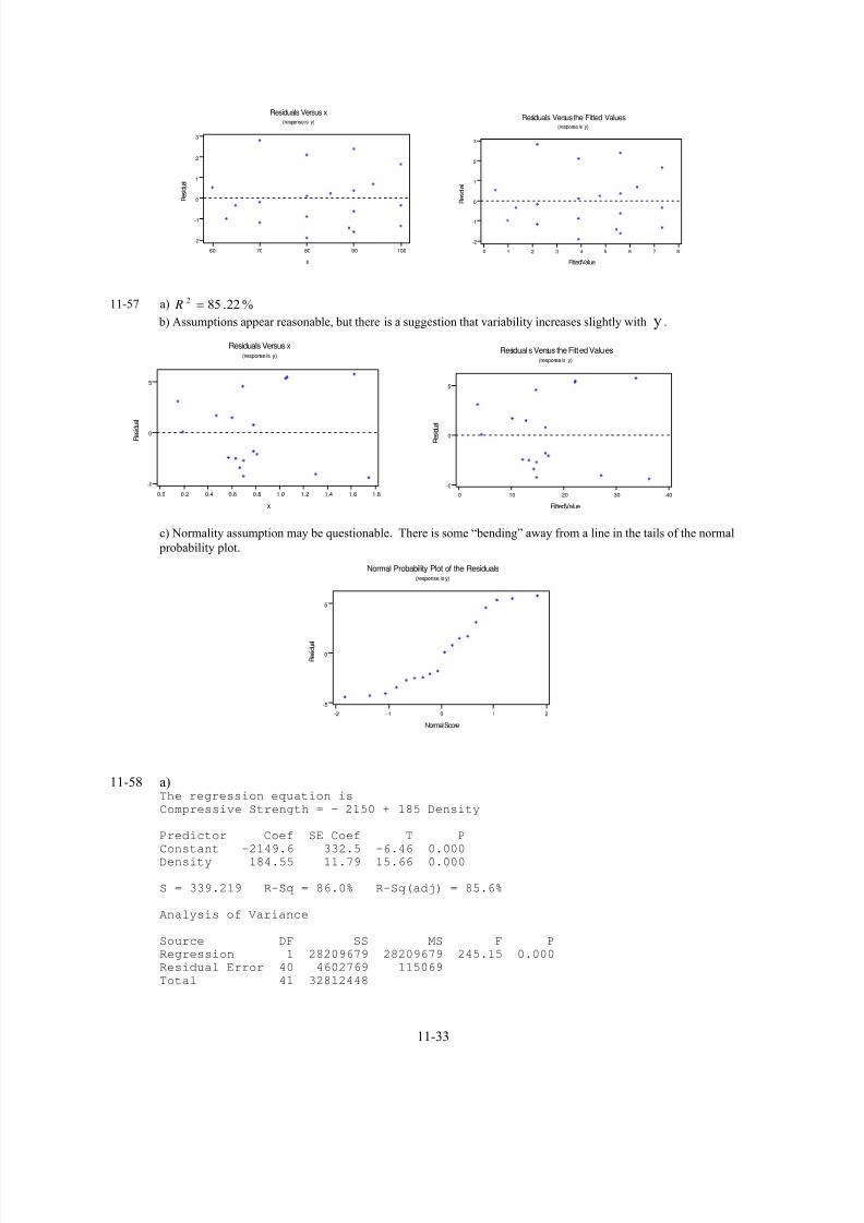
7/12/2019 Solution Manual Stats
http://slidepdf.com/reader/full/solution-manual-stats 345/588
11-33
10090807060
3
2
1
0
-1
-2
x
R e s i d u a l
Residuals Versus x(response is y)
876543210
3
2
1
0
-1
-2
FittedValue
R e s i d u a l
Residuals Versusthe Fitted Values(response is y)
11-57 a) %22.852= R
b) Assumptions appear reasonable, but there is a suggestion that variability increases slightly with y .
1.81.61.41.21.00.80.60.40.20.0
5
0
-5
x
R e s i d u a l
Residuals Versus x(response is y)
403020100
5
0
-5
FittedValue
R e s i d u a l
Residuals Versus the Fitted Values(response is y)
c) Normality assumption may be questionable. There is some “bending” away from a line in the tails of the normal
probability plot.
210-1-2
5
0
-5
Normal Score
R e s i d u a l
Normal Probability Plot of the Residuals(response is y)
11-58 a)The regression equation is
Compressive Strength = - 2150 + 185 Density
Predictor Coef SE Coef T P
Constant -2149.6 332.5 -6.46 0.000
Density 184.55 11.79 15.66 0.000
S = 339.219 R-Sq = 86.0% R-Sq(adj) = 85.6%
Analysis of Variance
Source DF SS MS F P
Regression 1 28209679 28209679 245.15 0.000
Residual Error 40 4602769 115069
Total 41 32812448

7/12/2019 Solution Manual Stats
http://slidepdf.com/reader/full/solution-manual-stats 346/588
11-34
b) Because the P-value = 0.000 < α = 0.05, the model is significant.
c) 115069ˆ 2=σ
d) %97.858597.032812448
2820967912
===−==T
E
T
R
SS
SS
SS
SS R
The model accounts for 85.97% of the variability in the data.
e)
Residual
P e r c e n t
10005000-500-1000
99
95
90
80
70
60
50
40
30
20
10
5
1
Normal Probability Plot of t he Residuals(response is Compressive Strength)
No major departure from the normality assumption.
f)
Fitt ed Value
R e s i d
u a l
50004000300020001000
1000
500
0
-500
-1000
Residuals Versus the Fit ted Values(response is Compressive Strength)
Assumption of constant variance appears reasonable.
11-59 a) 896081.02= R 89% of the variability is explained by the model.
b) Yes, the two points with residuals much larger in magnitude than the others seem unusual.

7/12/2019 Solution Manual Stats
http://slidepdf.com/reader/full/solution-manual-stats 347/588
11-35
1000-100-200
2
1
0
-1
-2
N o r m a l S c o r e
Residual
Normal Probability Plot of the Residuals
(response is y)
c) 9573.02
modelew =n R
Larger, because the model is better able to account for the variability in the data with these two outlying data pointsremoved.
d) 21.9811ˆ 2
modeld =olσ
93.4022ˆ 2
modelnew =σ
Yes, reduced more than 50%, because the two removed points accounted for a large amount of the error.
11-60 a)
1050950850
60
50
40
x
y
x y 0521753.0677559.0ˆ +=
b) 0: 10 = β H 0: 11 ≠ β H α = 0.05
12,1,0
12,1,05.
0
75.4
9384.7
α f f
f
f
>
=
=
Reject Ho.
c) 23842.25ˆ 2=σ
d) 502.7ˆ2
=origσ
The new estimate is larger because the new point added additional variance that was not accounted for by the model.
e) ˆ 0.677559 0.0521753(855) 45.287 y = + =
ˆ 59 45.287 13.713e y y= − = − =
Yes, e14 is especially large compared to the other residuals.
f) The one added point is an outlier and the normality assumption is not as valid with the point included.

7/12/2019 Solution Manual Stats
http://slidepdf.com/reader/full/solution-manual-stats 348/588
11-36
210-1-2
10
0
-10
Normal Score
R
e s i d u a l
Normal Probability Plot of the Residuals(response is y)
g) Constant variance assumption appears valid except for the added point.
1050950850
10
0
-10
x
R e s i d u a l
Residuals Versusx(response is y)
555045
10
0
-10
FittedValue
R e s i d u a l
Residuals Versus the Fitted Values(response is y)
11-61 Yes, when the residuals are standardized the unusual residuals are easier to identify.
1.0723949 -0.7005724 -0.1382218 0.6488043 -2.3530824 -2.1686819 0.4684192
0.4242137 0.0982116 0.5945823 0.2051244 -0.8806396 0.7921072 0.7242900
-0.4737526 0.9432146 0.1088859 0.3749259 1.0372187 -0.7774419
11-62 For two random variables X1 and X2,
),(2)()()( 212121 X X Cov X V X V X X V ++=+
Then,
[ ][ ] [ ]
[ ])(1
2
2)ˆˆ(
)ˆ,(2)ˆ()()ˆ(
2
22
2
)(12
)(12)(122
)(12
10
2
xx
i
xx
i
xx
i
xx
i
S
x x
n
S
x x
nS
x x
n
S
x x
ni
iiiiii
xV
Y Y CovY V Y V Y Y V
−
−−
−
+−=
+−++=
+−++=
−+=−
σ
σ σ σ
σ β β σ
a) Because ei is divided by an estimate of its standard error (when2σ is estimated by σ
2 ), r i has approximately unit
variance.
b) No, the term in brackets in the denominator is necessary.
c) If xi is near x and n is reasonably large, r i is approximately equal to the standardized residual.
d) If xi is far from x , the standard error of ei is small. Consequently, extreme points are better fit by least squares
regression than points near the middle range of x. Because the studentized residual at any point has variance of
approximately one, the studentized residuals can be used to compare the fit of points to the regression line over therange of x.
11-63 Using ,12
yy
E
S
SS R −=
2
2
0ˆ
)1)(2(
σ
E yy
n
SS
E yy
S
SS
S
SSSSSSSSn
F E
yy
E
yy
E −
=−
=−−
=−
Also,

7/12/2019 Solution Manual Stats
http://slidepdf.com/reader/full/solution-manual-stats 349/588
11-37
22
1
22
1
2
1
22
1
2
1
2
10
)(ˆ
)(ˆ)(
))((ˆ2)(ˆ)(
))(ˆ(
)ˆˆ(
x xSSS
x x y y
x x y y x x y y
x x y y
x ySS
i E yy
ii
iiii
ii
ii E
−=−
−−−=
−−−−+−=
−−−=
−−=
∑
∑∑
∑∑∑
∑
∑
β
β
β β
β
β β
Therefore, 2
02
2
10
/ˆ
ˆt
SF
xx
==σ
β
Because the square of a t random variable with n-2 degrees of freedom is an F random variable with 1 and n-2 degrees
of freedom, the usually t -test that compares || 0t to 2,2/ −nt α is equivalent to comparing2
00 t f = to
2
2,1, 2,2/ −=
− nt f n α α .
a) 2079.01
)23(9.00 =
−= f . Reject 0: 10 = β H .
b) Because 28.423,1,05. = f , 0 H is rejected if 28.4
1
232
2
>
− R
R .
That is, H0 is rejected if
157.0
28.428.27
)1(28.423
2
2
22
>
>
−>
R
R
R R

7/12/2019 Solution Manual Stats
http://slidepdf.com/reader/full/solution-manual-stats 350/588
11-38
Section 11-8
11-64 a) 0:0 = ρ H
0:1 ≠ ρ H α = 0.05
18,025.00
18,025.0
64.01
2208.0
0
||
101.2
657.5
t t
t
t
>
=
==−
−
Reject H0. P-value = (<0.0005)(2) = <0.001
b) 5.0:0 = ρ H
5.0:1 ≠ ρ H α = 0.05
2/0
025.
2/1
0
||
96.1
265.2)17)(0.5)(arctanh0.8)((arctanh
α z z
z
z
>
=
=−=
Reject H0. P-value = (0.012)(2) = 0.024.
c) )+0.8nhtanh(arcta)-0.8nhtanh(arcta1717
025.025. z z≤≤ ρ
where z. .025 196= . 9177.05534.0 ≤≤ ρ .
Because ρ = 0 and ρ = 0.5 are not in the interval, so reject H0.
11-65 a) 0:0 = ρ H
0:1 > ρ H α = 0.05
18,05.00
18,05.0
75.01
22075.0
0
734.1
81.42
t t
t
t
>
=
==−
−
Reject H0. P-value < 0.0005
b) 5.0:0 = ρ H
5.0:1 > ρ H α = 0.05
α z z
z
z
>
=
=−=
0
05.
2/1
0
65.1
7467.1)17)(0.5)(arctanh0.75)((arctanh
Reject H0. P-value = 0.04
c) )0.75nhtanh(arcta17
05.0 z−≥ ρ where 64.105. = z
26.2≥ ρ
Because ρ = 0 and ρ = 0.5 are not in the interval, reject the nul hypotheses from parts (a) and (b).
11-66 n = 25 r = 0.83
a) 0:0 = ρ H
0:1 ≠ ρ H α = 0.05

7/12/2019 Solution Manual Stats
http://slidepdf.com/reader/full/solution-manual-stats 351/588
11-39
23,2/0
23,025.
)83.0(1
2383.0
1
2
0
069.2
137.722
α t t
t
t r
nr
>
=
===−−
−
Reject H0 . P-value = 0.
b) )+0.83nhtanh(arcta)-0.83nhtanh(arcta2222
025.025. z z ≤≤ ρ
where z. .025 196= . 9226.06471.0 ≤≤ ρ .
a) 8.0:0 = ρ H
8.0:1 ≠ ρ H α = 0.05
2/0
025.
2/1
0
96.1
4199.0)22)(8.0arctanh83.0(arctanh
α z z
z
z
>/
=
=−=
Do not reject H0. P-value = (0.3373)(2) = 0.6746.
11-67 n = 50 r = 0.62
a) 0:0 = ρ H
0:1 ≠ ρ H α = 0.01
48,005.00
48,005.
)62.0(1
4862.0
1
2
0
682.2
475.522
t t
t
t r
nr
>
=
===−−
−
Reject H0. P-value ≅ 0
b) )+0.62nhtanh(arcta)-0.62nhtanh(arcta4747
005.005. z z ≤≤ ρ
where 575.2005.0 = z . 8007.03358.0 ≤≤ ρ .
c) Yes.
11-68 a) r = 0.933203
b) 0:0 = ρ H
0:1 ≠ ρ H α = 0.05
15,2/0
15,025.
)8709.0(1
15933203.0
1
2
0
131.2
06.102
α t t
t
t r
nr
>
=
===−−
−
Reject H0.
c) x y 498081.072538.0ˆ +=
0: 10 = β H
0: 11≠ β H α = 0.05
15,1,0
15,1,05.
0
543.416.101
α f f
f f
>>
==
Reject H0. Conclude that the model is significant at α = 0.05. This test and the one in part b) are identical.
d) No problems with model assumptions are noted.
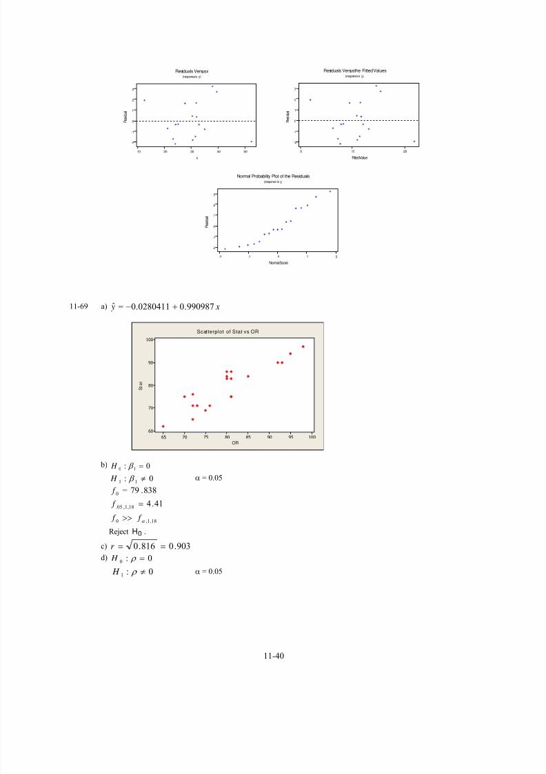
7/12/2019 Solution Manual Stats
http://slidepdf.com/reader/full/solution-manual-stats 352/588
11-40
5040302010
3
2
1
0
-1
-2
x
R e s i d u a l
Residuals Versusx(response is y)
25155
3
2
1
0
-1
-2
FittedValue
R e s i d u a l
Residuals Versusthe Fitted Values(response is y)
210-1-2
3
2
1
0
-1
-2
Normal Score
R e s i d u a l
Normal Probability Plot of the Residuals(response is y)
11-69 a) x y 990987.00280411.0ˆ +−=
OR
S t a t
10095908580757065
100
90
80
70
60
Scatterplot of Stat vs OR
b) 0: 10 = β H
0: 11 ≠ β H α = 0.05
18,1,0
18,1,05.
0
41.4
838.79
α f f
f
f
>>
=
=
Reject H0 .c) 903.0816.0 ==r
d) 0:0 = ρ H
0:1 ≠ ρ H α = 0.05

7/12/2019 Solution Manual Stats
http://slidepdf.com/reader/full/solution-manual-stats 353/588
11-41
18,2/0
18,025.
20
101.2
9345.8816.01
1890334.0
1
2
α t t
t
R
n Rt
>
=
=−
=−
−=
Reject H0.
e)5.0:0
= ρ H
5.0:1 ≠ ρ H α = 0.05
2/0
025.
0
96.1
879.3
α z z
z
z
>
=
=
Reject H0.
f) )+0.90334nhtanh(arcta)-0.90334nhtanh(arcta1717
025.025. z z ≤≤ ρ where 96.1025.0 = z .
9615.07677.0 ≤≤ ρ .
11-70 a) x y 419415.01044.69ˆ +=
b) 0: 10 = β H
0: 11≠ β H
α= 0.05
24,1,0
24,1,05.
0
260.4
744.35
α f f
f
f
>
=
=
Reject H0.
c) 77349.0=r
d) 0:0 = ρ H
0:1 ≠ ρ H α = 0.05
24,2/0
24,025.
5983.01
2477349.0
0
064.2
9787.5
α t t
t
t
>
=
==−
Reject H0.
e) 6.0:0 = ρ H
6.0:1 ≠ ρ H α = 0.05
2/0
025.
2/1
0
96.1
6105.1)23)(6.0arctanh77349.0(arctanh
α z z
z
z
>/
=
=−=
Do not reject H0 .
f) )+0.77349nhtanh(arcta)-0.77349nhtanh(arcta2323
025.025. z z ≤≤ ρ where z. .025 196= .
8932.05513.0 ≤≤ ρ .
11-71 a)

7/12/2019 Solution Manual Stats
http://slidepdf.com/reader/full/solution-manual-stats 354/588
11-42
Supply Voltage
C u r r e n t W i t h o
u t E l e c t ( m A )
76543210
50
40
30
20
10
Scatt erplot of Current WithoutElect(mA) vs Supply Voltage
The regression equation is
Current WithoutElect(mA) = 5.50 + 6.73 Supply Voltage
Predictor Coef SE Coef T P
Constant 5.503 3.104 1.77 0.114
Supply Voltage 6.7342 0.7999 8.42 0.000
S = 4.59061 R-Sq = 89.9% R-Sq(adj) = 88.6%
Analysis of Variance
Source DF SS MS F P
Regression 1 1493.7 1493.7 70.88 0.000
Residual Error 8 168.6 21.1
Total 9 1662.3
x y 73.650.5ˆ +=
Yes, because the P-value ≈ 0, the regression model is significant at α = 0.05.
b) 948.0899.0 ==r
c)
306.2425.8
306.2
425.8948.01
210948.0
1
2
0:
0:
8,025.00
8,025.0
220
1
0
=>=
=
=−
−=
−
−=
≠
=
t t
t
r
nr t
H
H
ρ
ρ
Reject H0.
d)

7/12/2019 Solution Manual Stats
http://slidepdf.com/reader/full/solution-manual-stats 355/588
11-43
9879.07898.0
310
6.19948.0harctantanh
310
96.1948.0harctantanh
3harctantanh
3harctantanh 2/2/
≤≤
⎟⎟ ⎠
⎞⎜⎜⎝
⎛
−+≤≤⎟⎟
⎠
⎞⎜⎜⎝
⎛
−−
⎟⎟ ⎠
⎞⎜⎜⎝
⎛
−+≤≤⎟⎟
⎠
⎞⎜⎜⎝
⎛
−−
ρ
ρ
ρ α α
n
zr
n
zr
11-72 a)
2000
2 0 0 1
1615141312
16
15
14
13
12
Scatterplot of 2001 vs 2000
The regression equation is
Y2001 = - 0.014 + 1.01 Y2000
Predictor Coef SE Coef T P
Constant -0.0144 0.3315 -0.04 0.966
Y2000 1.01127 0.02321 43.56 0.000
S = 0.110372 R-Sq = 99.5% R-Sq(adj) = 99.4%
Analysis of Variance
Source DF SS MS F P
Regression 1 23.117 23.117 1897.63 0.000
Residual Error 10 0.122 0.012
Total 11 23.239
x y 011.1014.0ˆ +−=
Yes, because the P-value ≈ 0, the regression model is significant at α = 0.05.
b) 9975.0995.0 ==r
c)

7/12/2019 Solution Manual Stats
http://slidepdf.com/reader/full/solution-manual-stats 356/588
11-44
( )
( )
025.00
025.02/
0
2/1
0
2/1
00
1
0
||
96.1
6084.5
312)9.0harctan9975.0h(arctan
3)harctanh(arctan
9.0:
9.0:
z z
z z
z
z
n R z
H
H
>
==
=−−=
−−=
≠
=
α
ρ
ρ
ρ
Reject H0. P-value = (1-1)(2) = 0.000.
d)
9993.09908.0
3126.199975.0harctantanh
31296.19975.0harctantanh
3harctantanh
3harctantanh 2/2/
≤≤
⎟⎟ ⎠ ⎞⎜⎜
⎝ ⎛
−+≤≤⎟⎟
⎠ ⎞⎜⎜
⎝ ⎛
−−
⎟⎟ ⎠
⎞⎜⎜⎝
⎛
−+≤≤⎟⎟
⎠
⎞⎜⎜⎝
⎛
−−
ρ
ρ
ρ α α
n
zr
n
zr
11-73 a) r= 787.0 =0.887
b)
0:
0:
1
0
≠
=
ρ
ρ
H
H
164.10887.01
230887.0
1
2
220=−
−
=−
−
= r
nr
t
28,025.0
28,025. 048.2
t t
t
>
=
Reject H0. The P-value < 0.0005
c)
9452.07741.0
330
6.19887.0harctantanh
330
96.1887.0harctantanh
≤≤
⎟⎟ ⎠
⎞⎜⎜⎝
⎛
−+≤≤⎟⎟
⎠
⎞⎜⎜⎝
⎛
−−
ρ
ρ
d)

7/12/2019 Solution Manual Stats
http://slidepdf.com/reader/full/solution-manual-stats 357/588
( )
( )
025.00
025.02/
0
2/1
0
2/1
00
1
0
||
96.1
808.2
312)7.0harctan887.0h(arctan
3)harctanh(arctan
7.0:
7.0:
z z
z z
z
z
n R z
H
H
>
==
=
−−=
−−=
≠
=
α
ρ
ρ
ρ
Reject H0. The P-value = 2(0.0025) = 0.005
11-74
x
y
43210-1-2-3-4-5
4
3
2
1
0
-1
-2
-3
-4
-5
Scatt erplot of y vs x
r = 0. The correlation coefficient does not detect the relationship between x and y because the relationshipis not linear as shown on the graph above.

7/12/2019 Solution Manual Stats
http://slidepdf.com/reader/full/solution-manual-stats 358/588
11-45
Section 11-9
11-75 a) Yes, ε β β lnlnlnln 10 ++= x y
b) No
c) Yes, ε β β lnlnlnln 10 ++= x y
d) Yes, ε β β ++=
x y
1110
11-76 a) There is curvature in the data.
38 033 028 0
80 0
70 0
60 0
50 0
40 0
30 0
20 0
10 0
0
Temperature (K)
V a p o r P r e s s u r e ( m m H
g )

7/12/2019 Solution Manual Stats
http://slidepdf.com/reader/full/solution-manual-stats 359/588
11-46
b) y = - 1956.3 + 6.686 x
c)Source DF SS MS F P
Regression 1 491662 491662 35.57 0.000Residual Error 9 124403 13823
Total 10 616065
d) There is a curve in the residuals.
e) The data are linear after the transformation to y* = ln y and x* = 1/ x.
ln y = 20.6 - 5201(1/x)
3500300025002000150010005000
15
10
5
0
x
y
-200 -100 0 100 200 300 400 500 600
-100
0
100
200
Fitted Value
R e s i d u a l
Residuals Versus the Fitted Values
(response is Vapor Pr)
0.00370.00320.0027
7
6
5
4
3
2
1
1/T
L n ( V P )

7/12/2019 Solution Manual Stats
http://slidepdf.com/reader/full/solution-manual-stats 360/588
11-47
Analysis of Variance
Source DF SS MS F PRegression 1 28.511 28.511 66715.47 0.000Residual Error 9 0.004 0.000Total 10 28.515
1 2 3 4 5 6 7
-0.03
-0.02
-0.01
0.00
0.01
0.02
Fitted Value
R e s i d u a l
Residuals Versus the Fitted Values
(response is y*)
There is still curvature in the data, but now the plot is convex instead of concave.
11-77 a)
3500300025002000150010005000
15
10
5
0
x
y
b) x y 00385.08819.0ˆ +−=
c) 0: 10 = β H
0: 11 ≠ β H α = 0.05
48,1,05.00
0 03.122
f f
f
>
=
Reject H0. Conclude that regression model is significant atα
= 0.05d) No, it seems the variance is not constant, there is a funnel shape.

7/12/2019 Solution Manual Stats
http://slidepdf.com/reader/full/solution-manual-stats 361/588
11-48
1050
3
2
1
0
-1
-2
-3
-4
-5
Fitted Value
R e s i d u a l
Residuals Versus the Fitted Values(response is y)
e) x y 00097.05967.0ˆ +=∗
. Yes, the transformation stabilizes the variance.

7/12/2019 Solution Manual Stats
http://slidepdf.com/reader/full/solution-manual-stats 362/588
11-49
Supplemental Exercises
11-78 a) ∑∑∑===
−=−n
i
i
n
i
i
n
i
ii y y y y
111
ˆ)ˆ( and ∑∑ += ii xn y 10ˆˆ β β from the normal equations
Then,
0ˆˆˆˆ
)ˆˆ(ˆˆ
ˆ)ˆˆ(
1
10
1
10
1
10
1
10
1
10
=−−+=
+−+=
−+
∑∑
∑∑
∑∑
==
==
=
n
i
i
n
i
i
n
i
i
n
i
i
i
n
i
i
xn xn
x xn
y xn
β β β β
β β β β
β β
b) i
n
iii
n
iii
n
iii x y x y x y y ∑∑∑
===
−=−111
ˆ)ˆ(
and ∑∑∑===
+=n
ii
n
iii
n
ii x x x y
1
21
10
1
ˆˆ β β from the normal equations. Then,
0ˆˆˆˆ
)ˆˆ(ˆˆ
1
21
10
1
21
10
1011
21
10
=−−+
=+−+
∑∑∑∑
∑∑∑
====
===
n
ii
n
ii
n
ii
n
ii
ii
n
i
n
ii
n
ii
x x x x
x x x x
β β β β
β β β β
c) y yn
n
i
i =∑=1
ˆ1
)ˆˆ(ˆ10 x y β β ∑ ∑ +=
y
x x y
x xn ynn
x x ynn
xnn
xn
yn
i
i
i
i
n
ii
=
+−=
+−=
+−=
+=
+=
∑
∑∑
∑∑=
1
11
11
10
101
ˆˆ
)ˆˆ(1
)ˆ)ˆ((1
)
ˆˆ
(
1
)ˆˆ(1
ˆ1
β β
β β
β β
β β
β β

7/12/2019 Solution Manual Stats
http://slidepdf.com/reader/full/solution-manual-stats 363/588
11-50
11-79 a)
1.1 1.3 1.5 1.7 1.9 2.1
x
0.7
1
1.3
1.6
1.9
2.2
y
Plot of y vs x
Yes, a linear relationship seems plausible.
b) Model fitting results for: y
Independent variable coefficient std. error t-value sig.level
CONSTANT -0.966824 0.004845 -199.5413 0.0000x 1.543758 0.003074 502.2588 0.0000
--------------------------------------------------------------------------------
R-SQ. (ADJ.) = 1.0000 SE= 0.002792 MAE= 0.002063 DurbWat= 2.843
Previously: 0.0000 0.000000 0.000000 0.000
10 observations fitted, forecast(s) computed for 0 missing val. of dep. var.
. .y x= − +0966824 154376
c) Analysis of Variance for the Full Regression
Source Sum of Squares DF Mean Square F-Ratio P-value
Model 1.96613 1 1.96613 252264. .0000
Error 0.0000623515 8 0.00000779394
--------------------------------------------------------------------------------
Total (Corr.) 1.96619 9
R-squared = 0.999968 Stnd. error of est. = 2.79176E-3
R-squared (Adj. for d.f.) = 0.999964 Durbin-Watson statistic = 2.84309
2) H0 1 0:β =
3) H1 1 0:β ≠
4) α = 0.05
5) The test statistic is)/(
/0
pnSS
k SS f
E
R
−=
6) Reject H0 if f 0 > f α,1,8 where f 0.05,1,8 = 5.32
7) Using the results from the ANOVA table
9.2552638/0000623515.0
1/96613.10 == f
8) Because 2552639 > 5.32 reject H0 and conclude that the regression model is significant at α = 0.05.
P-value < 0.000001
d) 95 percent confidence intervals for coefficient estimates
--------------------------------------------------------------------------------
Estimate Standard error Lower Limit Upper Limit
CONSTANT -0.96682 0.00485 -0.97800 -0.95565
x 1.54376 0.00307 1.53667 1.55085
--------------------------------------------------------------------------------
11.53667 1.55085 β ≤ ≤
e) 2) H0 0 0:β =

7/12/2019 Solution Manual Stats
http://slidepdf.com/reader/full/solution-manual-stats 364/588
11-51
3) H1 0 0:β ≠
4) α = 0.05
5) The test statistic is tse
00
0
=
( )
β
β
6) Reject H0 if t0 < −tα/2,n-2 where −t0.025,8 = −2.306 or t0 > t0.025,8 = 2.306
7) Using the results from the table above
t00 96682
000485199 34= − = −
.
..
8) Since −199.34 < −2.306 reject H0 and conclude the intercept is significant at α = 0.05.
11-80 a) x y 64.1534.93ˆ +=
b) 0: 10 = β H
0: 11 ≠ β H α = 0.05
14,1,05.00
14,1,05.
0
60.4
872.12
f f
f
f
>
=
=
Reject H0. Conclude that β1 0≠ at α = 0.05.
c) )322.23961.7( 1 ≤≤ β
d) )923.111758.74( 0 ≤≤ β
e) 44.132)5.2(64.1534.93ˆ =+= y
[ ]
91.138ˆ97.125
468.644.132
27.136145.244.132
5.2|
017.7
)325.25.2(
161
0
2
≤≤
±
+±
=
−
xY μ
11-81 x y 5075.02232.1ˆ +=∗where y y /1=∗
. No, the model does not seem reasonable.
The residual plots indicate a possible outlier.
11-82 x y 2047.25755.4ˆ += , r = 0.992, R 2
= 98.40%
The model appears to be an excellent fit. The R 2
is large and both regression coefficients are significant. No, the
existence of a strong correlation does not imply a cause and effect relationship.
11-83 x y 7916.0ˆ =
Even though y should be zero when x is zero, because the regressor variable does not usually assume values near zero, a
model with an intercept fits this data better. Without an intercept, the residuals plots are not satisfactory.
11-84 a)
181716
110
100
90
80
70
60
50
40
30
index
d a y s

7/12/2019 Solution Manual Stats
http://slidepdf.com/reader/full/solution-manual-stats 365/588
11-52
b) The regression equation is
x y 296.15193ˆ +−=
Analysis of VarianceSource DF SS MS F P
Regression 1 1492.6 1492.6 2.64 0.127
Residual Error 14 7926.8 566.2
Total 15 9419.4
Do not reject Ho. We do not have evidence of a relationship. Therefore, there is not sufficient evidence to conclude that
the seasonal meteorological index ( x) is a reliable predictor of the number of days that the ozone level exceeds 0.20
ppm ( y).
c) 95% CI on β1
504.35912.4
)421.9(145.2296.15
)421.9(296.15
)ˆ(ˆ
1
12,025.
12,2/1
≤≤−
±
±
± −
β
β β α
t
set n
d) The normality plot of the residuals is satisfactory. However, the plot of residuals versus run order exhibits a strong
downward trend. This could indicate that there is another variable should be included in the model and it is one that
changes with time.
11-85 a)
b) x y 29646714.0ˆ −=
161412108642
40
30
20
10
0
-10
-20
-30
-40
Observation Order
R e s i d u a l
403020100-10-20-30-40
2
1
0
-1
-2
N o r m a l S c o r e
Residual
1.00.90.80.70.60.50.40.3
0.7
0.6
0.5
0.4
0.3
0.2
x
y

7/12/2019 Solution Manual Stats
http://slidepdf.com/reader/full/solution-manual-stats 366/588
11-53
c) Analysis of Variance
Source DF SS MS F P
Regression 1 0.03691 0.03691 1.64 0.248
Residual Error 6 0.13498 0.02250
Total 7 0.17189
R 2 = 21.47%
Because the P-value > 0.05, reject the null hypothesis and conclude that the model is significant.
d) There appears to be curvature in the data. There is a dip in the middle of the normal probability plot and the plot of
the residuals versus the fitted values shows curvature.
11-86 a)
b) x y 9636.03.33ˆ +=
c)Predictor Coef SE Coef T P
Constant 66.0 194.2 0.34 0.743
Therm 0.9299 0.2090 4.45 0.002
S = 5.435 R-Sq = 71.2% R-Sq(adj) = 67.6%
Analysis of Variance
Source DF SS MS F P
Regression 1 584.62 584.62 19.79 0.002
Residual Error 8 236.28 29.53Total 9 820.90
Reject the null hypothesis and conclude that the model is significant. Here 77.3% of the variability is explained by the
model.
d) 1: 10 = β H
1: 11 ≠ β H α = 0.05
0.20.10.0-0.1-0.2
1.5
1.0
0.5
0.0
-0.5
-1.0
-1.5
N o r m a l S c o r e
Residual
0.4 0.5 0.6
-0.2
-0.1
0.0
0.1
0.2
Fitted Value
R e s i d u a l
920 930 940
920
930
940
x
y

7/12/2019 Solution Manual Stats
http://slidepdf.com/reader/full/solution-manual-stats 367/588
11-54
3354.02090.0
19299.0
)ˆ(
1ˆ
1
10 −=
−=
−=
β
β
set
306.28,025.2,2/ ==− t t na
Because 2,2/0 −−> nat t , we cannot reject H o and we conclude that there is not enough evidence to reject the claimthat the devices produce different temperature measurements. Therefore, we assume the devices produce equivalent
measurements.
e) The residual plots to not reveal any major problems.
-5 0 5
-1
0
1
N o r m a l S c o r e
Residual
Normal Probability Plot of the Residuals
(response is IR)
920 930 940
-5
0
5
Fitted Value
R e s i d u a l
Residuals Versus the Fitted Values
(response is IR)
11-87 a)
2 3 4 5 6 7
1
2
3
4
5
6
7
8
x
y

7/12/2019 Solution Manual Stats
http://slidepdf.com/reader/full/solution-manual-stats 368/588
11-55
b) x y 66.1699.0ˆ +−=
c)Source DF SS MS F P
Regression 1 28.044 28.044 22.75 0.001
Residual Error 8 9.860 1.233
Total 9 37.904
Reject the null hypothesis and conclude that the model is significant.
d) x0 = 4.25 257.4ˆ0| = x yμ
)3717.0(306.2257.4
625.20
)75.425.4(
10
12324.1306.2257.4
2
±
⎟⎟ ⎠
⎞⎜⎜⎝
⎛ −+±
114.5399.3 | ≤≤o x yμ
e) The normal probability plot of the residuals appears linear, but there are some large residuals in the lower fitted
values. There may be some problems with the model.
11-88 a)The regression equation is
No. Of Atoms (x 10E9) = - 0.300 + 0.0221 power(mW)
Predictor Coef SE Coef T P
Constant -0.29989 0.02279 -13.16 0.000
power(mW) 0.0221217 0.0006580 33.62 0.000
S = 0.0337423 R-Sq = 98.9% R-Sq(adj) = 98.8%
Analysis of Variance
Source DF SS MS F P
Regression 1 1.2870 1.2870 1130.43 0.000
Residual Error 13 0.0148 0.0011
Total 14 1.3018
8765432
2
1
0
-1
-2
Fitted Value
R e s i d u a l
-2 -1 0 1 2
-1
0
1
N o r m a l S c o r e
Residual

7/12/2019 Solution Manual Stats
http://slidepdf.com/reader/full/solution-manual-stats 369/588
11-56
power(mW)
N o .
O f A t o m s ( x
1 0 E 9 )
5040302010
0.8
0.6
0.4
0.2
0.0
S 0.0337423
R-Sq 98.9%
R-Sq(adj) 98.8%
Fitted Line PlotNo. Of Atoms (x 10E9) = - 0.2999 + 0.02212 power(mW)
b) Yes, there is a significant regression at α = 0.05 because p-value = 0.000 < α.
c) 994.0989.0 ==r
d)
.160.2766.32
160.2
766.32994.1
215994.0
1
2
0:
0:
13,025.00
13,025.0
220
1
0
=>=
=
=−
−=
−
−=
≠
=
t t
t
r
nr t
H
H
ρ
ρ
Reject H0. P-value = 0.000.
e) 95% confidence interval for 1
ˆ β
0234.0ˆ0206.0
)00066.0(160.2022.0
)00066.0(022.0
)ˆ(ˆ
1
13,025.0
12,2/1
≤≤
±
±
± −
β
β β α
t
set n
11-89 a)

7/12/2019 Solution Manual Stats
http://slidepdf.com/reader/full/solution-manual-stats 370/588
11-57
carat
p
r i c e
0.500.450.400.350.30
3500
3000
2500
2000
1500
1000
Scatter plot of pri ce vs carat
The relationship between carat and price is not linear. Yes, there is one outlier, observation number 33.
b) The person obtained a very good price—high carat diamond at low price.
c) All the data
The regression equation is
price = - 1696 + 9349 carat
Predictor Coef SE Coef T P
Constant -1696.2 298.3 -5.69 0.000
carat 9349.4 794.1 11.77 0.000
S = 331.921 R-Sq = 78.5% R-Sq(adj) = 77.9%
Analysis of Variance
Source DF SS MS F P
Regression 1 15270545 15270545 138.61 0.000
Residual Error 38 4186512 110171
Total 39 19457057
tα/2,n-2 = t0.025,38 = 2.024
95% confidence interval on β1 .
.26.1095674.7741
)1.794(024.29349
)1.794(9349
)ˆ(ˆ
1
38,025.
12,2/1
≤≤
±
±
± −
β
β β α
t
set n
With unusual data omittedThe regression equation is
price_1 = - 1841 + 9809 carat_1
Predictor Coef SE Coef T PConstant -1841.2 269.9 -6.82 0.000
carat_1 9809.2 722.5 13.58 0.000
S = 296.218 R-Sq = 83.3% R-Sq(adj) = 82.8%
Analysis of Variance
Source DF SS MS F P
Regression 1 16173949 16173949 184.33 0.000

7/12/2019 Solution Manual Stats
http://slidepdf.com/reader/full/solution-manual-stats 371/588
11-58
Residual Error 37 3246568 87745
Total 38 19420517
tα/2,n-2 = t0.025,37 = 2.026
95% confidence interval on β1 .
79.1127222.8345
)5.722(026.29809)5.722(9809
)ˆ(ˆ
1
37,025.
12,2/1
≤≤
±±
± −
β
β β α
t
set n
The width for the outlier removed is narrower than for the first case.
11-90The regression equation is
Population = 3549143 + 651828 Count
Predictor Coef SE Coef T P
Constant 3549143 131986 26.89 0.000
Count 651828 262844 2.48 0.029
S = 183802 R-Sq = 33.9% R-Sq(adj) = 28.4%
Analysis of Variance
Source DF SS MS F P
Regression 1 2.07763E+11 2.07763E+11 6.15 0.029
Residual Error 12 4.05398E+11 33783126799
Total 13 6.13161E+11
x y 6518283549143ˆ +=
Yes, the regression is significant at α = 0.05. Care needs to be taken in making cause and effect statements
based on a regression analysis. In this case, it is surely not the case that an increase in the stork count iscausing the population to increase, in fact, the opposite is most likely the case. However, unless a designed
experiment is performed, cause and effect statements should not be made on regression analysis alone. The
existence of a strong correlation does not imply a cause and effect relationship.

7/12/2019 Solution Manual Stats
http://slidepdf.com/reader/full/solution-manual-stats 372/588
Mind-Expanding Exercises
12-98. Because
yy
R
S
SS R =2
and
yy
E
S
SS R =− 21 ,
)1/(
/0 −−
=k nSS
k SSF
E
Rand this is the usual F-test for significance
of regression. Then, 75.33)1420/()9.01(
4/90.00 =
−−−=F and the critical value is . Because
33.75 > 3.06, regression is significant.
f. , , .05 415 3 06=
12-73

7/12/2019 Solution Manual Stats
http://slidepdf.com/reader/full/solution-manual-stats 373/588
12-99. Using n = 20, k = 4, f . Reject H. , , .05 4 15 3 06= 0 if
816.0
)1(
06.315/)1(
4/
2
2
2
2
≥
−
≥−
R
R
R
R
Then, results in a significant regression.449.02 ≥ R
12-100. Because ,Y X X X ')'(ˆ 1−= β Y H I Y X X X X Y X Y e )(')'(ˆ 1 −=−=−= − β
12-101. From Exercise 12-76, ei is ith element of ( I - H )Y . That is,
22
,
2
1,
2
,
2
1,
2
2,
2
1,
,11,,11,22,11,
)...)1(...()(
...)1(...
σ niiiiiiiiii
nniiiiiiiiiiiii
hhhhhheV
and
Y hY hY hY hY hY he
+++−++++=
−−−−+−−−−=
+−
++−−
The expression in parentheses is recognized to be the ith diagonal element of ( I - H )( I - H ') = I - H by matrix
multiplication. Consequently, . Assume that i < j. Now,2
, )1()( σ iii heV −=
nn j j j j j j j j j j j j j
nniiiiiiiiiiiii
Y hY hY hY hY hY he
Y hY hY hY hY hY he
,11,,11,22,11,
,11,,11,22,11,
...)1(...
...)1(...
−−−−+−−−−=−−−−+−−−−=
++−−
++−−
Because the yi‘s are independent,
i jiii jii ji ji ji hhhhhhhheeCov ,,1,1,2,2,1,1, )1(...(),( −++++= −−
2
,,1,1,,,1,1, )...)1(... σ n jni j j ji j j jii jii
hhhhhhhh +++−+++ ++++
The expression in parentheses is recognized as the ijth element of ( I - H )( I - H ') = I - H . Therefore, .2),( σ ij ji heeCov −=
12-102. ε β ε β ε β β R X X X Y X X X +=+=+== − 'X)(X')('X)(X'')'(ˆ -1-11
12-103. a) Min L = )()'( β β X y X y −− subject to :Tβ = c
This is equivalent to Min Z = ( )' ( ) ' (y X y X T c)+ −β λ β2
where λ ],...,2
,1
[' pλ λ λ = is a vector of La Grange multipliers.
∂
∂ββ λ
ZX y X X T= − + +2 2 2' ( ' ) '
( )cT Z
−= β ∂λ
∂ 2 . Set
∂
∂β
∂
∂λ
Z Z= =0 0, .
Then we get
cT
y X T X X
c
c
=
=+
β
λ β
ˆ
''ˆ)'(
where is the constrained estimator. From the first of these equations,βc ( ' ) ( ' ' ) ( ' ) 'λ βc X X X y T X X T= − = −− λ−1 1
From the second,T T or λX X T ( ' ) 'λ− =−1 c = − −[ ( ' ) ' ]T X X T1 1(T - c)β
Then ( ' ) '[ ( ' ) ' ] ( )
( ' ) '[ ( ' ) ' ] ( )
β β β
β β
c X X T T X X T T c
X X T T X X T c T
= − −
= + −
− − −
− − −
1 1 1
1 1 1
12-74

7/12/2019 Solution Manual Stats
http://slidepdf.com/reader/full/solution-manual-stats 374/588
b) This solution would be appropriate in situations where you have tested the hypothesis that Tβ = c and concluded
that this hypothesis cannot be rejected.
12-104. a) For the piecewise linear function to be continuous at x = x , the point-slope formula for a line can be used to
show that
*
⎪⎩
⎪⎨
⎧
>−+
≤−+=
∗ x x x x
x x x x
y
)(
)(
*
20
**
10
β β
β β
where β β are arbitrary constants.β0 1 2, ,
Let .
⎪⎩
⎪⎨
⎧
>
≤=
∗
∗
x x
x x
z
,1
,0
Then, y can be written as . z x x x x y ))(()( 1210
∗∗ −−+−+= β β β β
Let
122
11
00
2
1
)(
β β β
β β
β β
−=
=
=
−=
−=
∗
∗
∗
∗
∗
z x x x
x x x
Then,22110
*** x x y β β β ++= .
b) Should refer to exercise 12-80. If there is a discontinuity at x x= ∗, then a model that can be used is
⎪⎩
⎪⎨
⎧
>+
≤+=
∗ x x x
x x x
y
10
*
10
α α
β β
Let
⎪⎩
⎪⎨
⎧
>
≤=
∗
∗
x x
x x
z
,1
,0
Then, y can be written as y x x z x z= + + − + − = + + + x∗ ∗ ∗ ∗β β α β α β β β β β0 1 0 0 1 1 0 1 1 2 3[( ) ( ) ] 2
where
xz x
x x
=
=
−=
−=
=
=
∗
∗
∗
∗
2
1
113
002
11
00
β α β
β α β
β β
β β
c) Should refer to exercise 12-80. One could estimate x* as a parameter in the model. A simple approach is to refit the
model in Exercise 12-80 with different choices for x* and to select the value for x* that minimizes the residual sum of
squares.
12-75

7/12/2019 Solution Manual Stats
http://slidepdf.com/reader/full/solution-manual-stats 375/588
CHAPTER 12
Sections 12-1
12-1. a) ′ =
⎡
⎣
⎢
⎢⎢
⎤
⎦
⎥
⎥⎥
X X
10 223 553
223 52009 12352
553 12352 31729
.
′ =
⎡
⎣
⎢⎢⎢
⎤
⎦
⎥⎥⎥
X y
19160
435508
104736 8
.
.
.
b) so
⎥⎥⎥
⎦
⎤
⎢⎢⎢
⎣
⎡
−
=
126.1
713.3
055.171
ˆ β 21 126.1714.3055.171ˆ x x y −+=
c) 49.189)43(126.1)18(714.3055.171ˆ =−+= y
12-2. a) y X X X ′′=−1
)(ˆ β
⎥⎥⎥
⎦
⎤
⎢⎢⎢
⎣
⎡−
=
2532.0
0931.0
9122.1
ˆ β
b) 21 2532.00931.09122.1ˆ x x y ++−=
3678.29)50(2532.0)200(0931.09122.1ˆ =++−= y
12-3. a) Model 1 Model 2
x2 2= y x= + +100 2 81 . ( )y x x= + + +95 15 3 2 41 1
x
x
x
y = +108 2 1
.y x= +101 55 1
x2 8= ( )y x= + +100 2 4 81 . ( )y x= + + +95 15 3 8 161 1
y = +132 2 1 .y x= +119 17 5 1
MODEL 1
0
20
40
60
80
100
120
140
160
0 2 4 6 8 1 0
x
y
y = 132 + 2
y = 108 + 2
12-1

7/12/2019 Solution Manual Stats
http://slidepdf.com/reader/full/solution-manual-stats 376/588
MODEL 2
0
50
100
150
200
250
300
350
0 5 10 15
x
yy = 101 + 5.5 x
y = 119 + 17.5 x
The interaction term in model 2 affects the slope of the regression equation. That is, it modifies the
amount of change per unit of onx1 y .
b) x2 5= ( )y x= + +100 2 4 51
y x= +120 2 1
Then, 2 is the expected change on y per unit of .x1
NO, it does not depend on the value of x2, because there is no relationship or interaction between these
two variables in model 1.
c) x2 5= x2 2= x2 8=
. ( ) (y x x= + + +95 15 3 5 2 51 1 )
.y x= +110 115 1
.y x= +101 55 1 .y x= +119 17 5 1
Change per
unit of x 1
11.5 5.5 17.5
Yes, result does depend on the value of x2, because x2 interacts with x1.
12-4. Predictor Coef SE Coef T P Constant -123.1 157.3 -0.78 0.459X1 0.7573 0.2791 2.71 0.030X2 7.519 4.010 1.87 0.103
X3 2.483 1.809 1.37 0.212X4 -0.4811 0.5552 -0.87 0.415
S = 11.79 R-Sq = 85.2% R-Sq(adj) = 76.8%
Analysis of Variance
Source DF SS MS F P
Regression 4 5600.5 1400.1 10.08 0.005Residual Error 7 972.5 138.9Total 11 6572.9
a) 4321 4811.0483.2519.77573.01.123ˆ x x x x y −+++−=
b) 00.139ˆ 2 =σ
c) , , , , and3.157)ˆ( 0 = β se 2791.0)ˆ( 1 = β se 010.4)ˆ( 2 = β se 809.1)ˆ( 3 = β se 5552.0)ˆ( 4 = β se
d) 476.290)98(4811.0)90(483.2)24(519.7)75(7573.01.123ˆ =−+++−= y
12-2

7/12/2019 Solution Manual Stats
http://slidepdf.com/reader/full/solution-manual-stats 377/588
12-5. The regression equation is mpg = 49.9 - 0.0104 cid - 0.0012 rhp - 0.00324 etw + 0.29 cmp - 3.86 axle
+ 0.190 n/v
Predictor Coef SE Coef T PConstant 49.90 19.67 2.54 0.024cid -0.01045 0.02338 -0.45 0.662
rhp -0.00120 0.01631 -0.07 0.942etw -0.0032364 0.0009459 -3.42 0.004cmp 0.292 1.765 0.17 0.871axle -3.855 1.329 -2.90 0.012n/v 0.1897 0.2730 0.69 0.498
S = 2.22830 R-Sq = 89.3% R-Sq(adj) = 84.8%
Analysis of Variance
Source DF SS MS F PRegression 6 581.898 96.983 19.53 0.000Residual Error 14 69.514 4.965Total 20 651.412
a) 654321 1897.0855.3292.000324.00012.001045.090.49ˆ x x x x x x y +−+−−−=
where vn xaxle xcmp xetw xrhp xcid x /654321 ======
b) 965.4ˆ 2 =σ
, , , ,67.19)ˆ( 0 = β se 02338.0)ˆ( 1 = β se 01631.0)ˆ( 2 = β se 0009459.0)ˆ( 3 = β se
, and765.1)ˆ( 4 = β se 329.1)ˆ( 5 = β se 273.0)ˆ( 6 = β se
c)
9.30(1897.0)07.3(855.3)9.9(292.0)4500(0032.0)253(0012.0)215(01045.090.49ˆ +−+−−−= y= 29.867
12-6. The regression equation is
y = 7.46 - 0.030 x2 + 0.521 x3 - 0.102 x4 - 2.16 x5Predictor Coef StDev T PConstant 7.458 7.226 1.03 0.320x2 -0.0297 0.2633 -0.11 0.912x3 0.5205 0.1359 3.83 0.002x4 -0.10180 0.05339 -1.91 0.077x5 -2.161 2.395 -0.90 0.382S = 0.8827 R-Sq = 67.2% R-Sq(adj) = 57.8% Analysis of VarianceSource DF SS MS F PRegression 4 22.3119 5.5780 7.16 0.002Error 14 10.9091 0.7792Total 18 33.2211
a) 5432 1606.21018.05205.00297.04578.7ˆ x x x x y −−+−= b) 7792.ˆ 2 =σ
c) , , , and226.7)ˆ( 0 = β se 2633.)ˆ( 2 = β se 1359.)ˆ( 3 = β se 05339.)ˆ( 4 = β se 395.2)ˆ( 5 = β se
d) )0.2(1606.2)90(1018.0)30(5205.0)20(0297.04578.7ˆ −−+−= y 996.8ˆ = y
12-7.
12-3

7/12/2019 Solution Manual Stats
http://slidepdf.com/reader/full/solution-manual-stats 378/588
Predictor Coef SE Coef T PConstant 47.82 49.94 0.96 0.353
x1 -9.604 3.723 -2.58 0.020x2 0.4152 0.2261 1.84 0.085x3 18.294 1.323 13.82 0.000 --------------------------------------------------------------------------------
a) 321 294.1844152.0604.982.47ˆ x x x y ++−=
b) 3.12ˆ 2 =σ
c) , , , and94.49)ˆ( 0 = β se 723.3)ˆ( 1 = β se 2261.0)ˆ( 2 = β se 323.1)ˆ( 3 = β se
d) 38.91)5(29.18)220(44152.0)5.14(604.982.47ˆ =++−= y
12-8. Predictor Coef SE Coef T PConstant -0.03023 0.06178 -0.49 0.629temp 0.00002856 0.00003437 0.83 0.414
soaktime 0.0023182 0.0001737 13.35 0.000soakpct -0.003029 0.005844 -0.52 0.609difftime 0.008476 0.001218 6.96 0.000diffpct -0.002363 0.008078 -0.29 0.772
S = 0.002296 R-Sq = 96.8% R-Sq(adj) = 96.2%
Analysis of Variance
Source DF SS MS F PRegression 5 0.00418939 0.00083788 158.92 0.000
Residual Error 26 0.00013708 0.00000527Total 31 0.00432647
a) 54321 002363.0008476.0003029.0002318.0000029.003023.0ˆ x x x x x y −+−++−=
where DIFFPCT x DFTIME xSOAKPCT xSOAKTIME xTEMP x ===== 54321
b) 62 1027.5ˆ −= xσ
c) The standard errors are listed under the StDev column above.
d)
)80.0(002363.0)1(008476.0
)1.1(003029.0)1(002318.0)1650(000029.003023.0ˆ
−+
−++−= y
02247.0ˆ = y
12-9. The regression equation is rads = - 440 + 19.1 mAmps + 68.1 exposure time
Predictor Coef SE Coef T PConstant -440.39 94.20 -4.68 0.000mAmps 19.147 3.460 5.53 0.000exposure time 68.080 5.241 12.99 0.000
S = 235.718 R-Sq = 84.3% R-Sq(adj) = 83.5%
Analysis of Variance
Source DF SS MS F PRegression 2 11076473 5538237 99.67 0.000Residual Error 37 2055837 55563Total 39 13132310
12-4

7/12/2019 Solution Manual Stats
http://slidepdf.com/reader/full/solution-manual-stats 379/588
a) 21 080.68147.1939.440ˆ x x y ++−=
where Time Exposure xmAmps x == 21
b) 55563ˆ 2 =σ
, , and20.94)ˆ( 0 = β se 460.3)ˆ( 1 = β se 241.5)ˆ( 2 = β se
c) 675.186)5(080.68)15(147.1993.440ˆ =++−= y
12-10. The regression equation is ARSNAILS = 0.488 - 0.00077 AGE - 0.0227 DRINKUSE - 0.0415 COOKUSE
+ 13.2 ARSWATER
Predictor Coef SE Coef T PConstant 0.4875 0.4272 1.14 0.271AGE -0.000767 0.003508 -0.22 0.830DRINKUSE -0.02274 0.04747 -0.48 0.638COOKUSE -0.04150 0.08408 -0.49 0.628ARSWATER 13.240 1.679 7.89 0.000
S = 0.236010 R-Sq = 81.2% R-Sq(adj) = 76.5%
Analysis of Variance
Source DF SS MS F PRegression 4 3.84906 0.96227 17.28 0.000Residual Error 16 0.89121 0.05570Total 20 4.74028
a) 4321 240.1304150.002274.0000767.04875.0ˆ x x x x y +−−−=
where ARSWater xCookUse x DrinkUse x AGE x ==== 4321
b) 05570.0ˆ 2 =σ
, , , , and4272.0)ˆ( 0= β se 003508.0)ˆ( 1
= β se 04747.0)ˆ( 2= β se 08408.0)ˆ( 3
= β se 679.1)ˆ( 4 = β se
c) 9307.1)135.0(240.13)5(04150.0)5(02274.0)30(000767.04875.0ˆ =+−−−= y
12-11. The regression equation is density = - 0.110 + 0.407 dielectric constant + 2.11 loss factor
Predictor Coef SE Coef T PConstant -0.1105 0.2501 -0.44 0.670dielectric constant 0.4072 0.1682 2.42 0.042loss factor 2.108 5.834 0.36 0.727
S = 0.00883422 R-Sq = 99.7% R-Sq(adj) = 99.7%
Analysis of Variance
Source DF SS MS F PRegression 2 0.23563 0.11782 1509.64 0.000Residual Error 8 0.00062 0.00008Total 10 0.23626
12-5

7/12/2019 Solution Manual Stats
http://slidepdf.com/reader/full/solution-manual-stats 380/588
a) 21 108.24072.01105.0ˆ x x y ++−=
where LossFactor xConst Dielectric x == 21
b) 00008.0ˆ 2 =σ
, , and2501.0)ˆ( 0 = β se 1682.0)ˆ( 1 = β se 834.5)ˆ( 2 = β se
c) 97074.0)03.0(108.2)5.2(4072.01105.0ˆ =++−= y
12-12. The regression equation is y = - 171 + 7.03 x1 + 12.7 x2
Predictor Coef SE Coef T PConstant -171.26 28.40 -6.03 0.001x1 7.029 1.539 4.57 0.004x2 12.696 1.539 8.25 0.000
S = 3.07827 R-Sq = 93.7% R-Sq(adj) = 91.6%
Analysis of Variance
Source DF SS MS F PRegression 2 842.37 421.18 44.45 0.000Residual Error 6 56.85 9.48Total 8 899.22
a) 21 7.1203.7171ˆ x x y ++−=
b) 48.9ˆ 2 =σ
, , and40.28)ˆ( 0 = β se 539.1)ˆ( 1 = β se 539.1)ˆ( 2 = β se
c) )5.12(7.12)5.14(03.7171ˆ ++−= y
= 89.685
12-13. The regression equation is Useful range (ng) = 239 + 0.334 Brightness (%) - 2.72 Contrast (%)
Predictor Coef SE Coef T PConstant 238.56 45.23 5.27 0.002Brightness (%) 0.3339 0.6763 0.49 0.639Contrast (%) -2.7167 0.6887 -3.94 0.008
S = 36.3493 R-Sq = 75.6% R-Sq(adj) = 67.4%
Analysis of Variance
Source DF SS MS F PRegression 2 24518 12259 9.28 0.015Residual Error 6 7928 1321Total 8 32446
a) 21 7167.23339.056.238ˆ x x y −+=
where Contrast x Brightness x %% 21 ==
b) 1321ˆ 2 =σ
12-6

7/12/2019 Solution Manual Stats
http://slidepdf.com/reader/full/solution-manual-stats 381/588
c) , , and23.45)ˆ( 0 = β se 6763.0)ˆ( 1 = β se 6887.0)ˆ( 2 = β se
d) 5195.61)75(7167.2)80(3339.056.238ˆ =−+= y
12-14. The regression equation is Stack Loss(y) = - 39.9 + 0.716 X1 + 1.30 X2 - 0.152 X3
Predictor Coef SE Coef T PConstant -39.92 11.90 -3.36 0.004X1 0.7156 0.1349 5.31 0.000X2 1.2953 0.3680 3.52 0.003X3 -0.1521 0.1563 -0.97 0.344
S = 3.24336 R-Sq = 91.4% R-Sq(adj) = 89.8%
Analysis of Variance
Source DF SS MS F PRegression 3 1890.41 630.14 59.90 0.000Residual Error 17 178.83 10.52
Total 20 2069.24
a) 321 1521.02953.17156.092.39ˆ x x x y −++−=
b) 52.10ˆ 2 =σ
c) , , , and90.11)ˆ( 0 = β se 1349.0)ˆ( 1 = β se 3680.0)ˆ( 2 = β se 1563.0)ˆ( 3 = β se
d) 7653.23)85(1521.0)26(2953.1)60(7156.092.39ˆ =−++−= y
12-15. The regression equation isRating Pts = 3.22 + 1.22 Pct Comp + 4.42 Pct TD - 4.09 Pct Int
Predictor Coef SE Coef T P
Constant 3.220 6.519 0.49 0.626Pct Comp 1.2243 0.1080 11.33 0.000Pct TD 4.4231 0.2799 15.80 0.000Pct Int -4.0914 0.4953 -8.26 0.000
S = 1.92094 R-Sq = 97.8% R-Sq(adj) = 97.5%
Analysis of Variance
Source DF SS MS F PRegression 3 4196.3 1398.8 379.07 0.000Residual Error 26 95.9 3.7Total 29 4292.2
a) 1073 091.4423.4224.122.3ˆ x x x y −++=
Where X3 = percentage of completions, X7 = percentage of TDs, and X10 = percentage of interceptions
b) 7.3ˆ 2 =σ
c) , , , and519.6)ˆ( 0 = β se 1080.0)ˆ( 3 = β se 2799.0)ˆ( 7 = β se 4953.0)ˆ( 10 = β se
d) 079.82)3(091.4)4(423.4)60(224.122.3ˆ =−++= y
12-16. Predictor Coef SE Coef T P
12-7

7/12/2019 Solution Manual Stats
http://slidepdf.com/reader/full/solution-manual-stats 382/588
Constant -29.46 93.98 -0.31 0.758GF 0.12356 0.05319 2.32 0.035GA -0.15953 0.04458 -3.58 0.003ADV 0.1236 0.2023 0.61 0.550PPGF -0.764 1.269 -0.60 0.556PCTG 3.100 4.406 0.70 0.492PEN 0.2402 0.3453 0.70 0.497BMI 0.0036 0.1151 0.03 0.976
AVG -18.86 28.31 -0.67 0.515SHT -0.03494 0.03419 -1.02 0.323PPGA 0.0526 0.2137 0.25 0.809PKPCT 0.0505 0.7221 0.07 0.945SHGF 0.5833 0.3935 1.48 0.159SHGA 0.3733 0.2712 1.38 0.189FG 0.1578 0.2227 0.71 0.489
S = 3.58133 R-Sq = 90.1% R-Sq(adj) = 80.9%
Analysis of Variance
Source DF SS MS F PRegression 14 1754.28 125.31 9.77 0.000Residual Error 15 192.39 12.83Total 29 1946.67
7654321 0036.02402.01.3764.01236.015953.012356.046.29ˆ x x x x x x x y +++−+−+−=
141312111098 1578.03733.05833.00505.00526.003494.086.18 x x x x x x x +++++−−
where
FG xSHGA xSHGF xPKPCT xPPGA xSHT x AVG x
BMI xPEN xPCTG xPPGF x ADV xGA xGF x
=======
=======
141312111098
7654321
83.12ˆ 2 =σ The standard errors of the coefficients are listed under the SE Coef column above.
12-17. Predictor Coef SE Coef T PConstant 383.80 36.22 10.60 0.002
Xl -3.6381 0.5665 -6.42 0.008X2 -0.11168 0.04338 -2.57 0.082S = 12.35 R-Sq = 98.5% R-Sq(adj) = 97.5%
Analysis of Variance
Source DF SS MS F PRegression 2 29787 14894 97.59 0.002Residual Error 3 458 153Total 5 30245
a) 21 1119.06381.380.383ˆ x x y −−=
b) , , , and0.153ˆ 2 =σ 22.36)ˆ( 0 = β se 5665.0)ˆ( 1 = β se 04338.)ˆ( 2 = β se
c) 95.180)1000(1119.0)25(6381.380.383ˆ =−−= y
d) Predictor Coef SE Coef T P
Constant 484.0 101.3 4.78 0.041Xl -7.656 3.846 -1.99 0.185
X2 -0.2221 0.1129 -1.97 0.188X1*X2 0.004087 0.003871 1.06 0.402S = 12.12 R-Sq = 99.0% R-Sq(adj) = 97.6%Analysis of VarianceSource DF SS MS F PRegression 3 29951.4 9983.8 67.92 0.015
Residual Error 2 294.0 147.0Total 5 30245.3
1221 0041.0222.0656.70.484ˆ x x x y −−−=
e) , , , and0.147ˆ 2 =σ 3.101)ˆ( 0 = β se 846.3)ˆ( 1 = β se 113.0)ˆ( 2 = β se 0039.0)ˆ( 12 = β se
12-8

7/12/2019 Solution Manual Stats
http://slidepdf.com/reader/full/solution-manual-stats 383/588
f) 1.173)1000)(25(0041.0)1000(222.0)25(656.70.484ˆ =−−−= y
The predicted value is smaller
12-18. a)2
222111
'
021
'
0 )]()([),,( x x x x y f iii −−−−−= ∑ β β β β β β
))](()([2
)]()([2
11222111
'
0
1
222111'0'
0
x x x x x x y f
x x x x y f
iiii
iii
−−−−−−−=
−−−−−−=
∑
∑
β β β ∂β
∂
β β β ∂β ∂
))](()([2 22222111
'
0
2
x x x x x x y f
iiii −−−−−−−= ∑ β β β ∂β
∂
Setting the derivatives equal to zero yields
)()()()(
)())(()(
222
22222111'0
1122112
2
111
'
0
'
0
x x y x x x x x xn
x x y x x x x x xn
yn
iiiii
iiiii
i
−=−+−−+
−=−−+−+
=
∑∑∑
∑∑∑∑
β β β
β β β
β
b) From the first normal equation, y='
0ˆ β .
c) Substituting y yi − for y in the first normal equation yields .i 0ˆ '
0 = β

7/12/2019 Solution Manual Stats
http://slidepdf.com/reader/full/solution-manual-stats 384/588
Sections 12-2
12-19. a) n = 10, k = 2, p = 3, α = 0.05
0...: 210 ==== k H β β β
0:1 ≠ j H β for at least one j
⎥⎥⎥
⎦
⎤
⎢⎢⎢
⎣
⎡=
⎥
⎥⎥
⎦
⎤
⎢
⎢⎢
⎣
⎡
=
=−=
∑∑∑
8.104736
8.43550
1916
'
449010
)1916(6.371595
2
1
2
ii
ii
i
yy
y x
y x
y
y X
S
[ ]
7.833.44064490
3.440610
19169.371511
9.371511
8.104736
8.43550
1916
126.1713.3055.171''ˆ
2
=−=−=
=−=
=
⎥⎥⎥
⎦
⎤
⎢⎢⎢
⎣
⎡−=
R yy E
R
SSSSS
SS
y X β
7,2,05.00
7,2,05.0
0
74.4
25.1847/7.83
2/3.4406
f f
f
f pn
SS
k
SS
E
R
>
=
===−
12-9

7/12/2019 Solution Manual Stats
http://slidepdf.com/reader/full/solution-manual-stats 385/588
Reject H0 and conclude that the regression model is significant at α = 0.05. P-value = 0.000
b) 957.11ˆ 2 =−
== pn
SS MS E
E σ
229.0)00439.0(957.11ˆ)ˆ(11
2
1 === cse σ β
10199.0)00087.0(957.11ˆ)ˆ( 22
2
2 === cse σ β
0: 10 = β H 02 = β
0: 11 ≠ β H 02 ≠ β
21.16229.0
713.3
)ˆ(
ˆ
1
10
==
= β
β
set
04.1110199.0
126.1
)ˆ(
ˆ
2
20
−=−
=
= β
β
set
365.27,025.07,2/ == t t α
Reject H0, P-value < 0.001 Reject H0, P-value < 0.001
Both regression coefficients significant
12-20. 00.742= yyS
a) 0: 210 == β β H
0:1 ≠ j H β for at least one j
α = 0.01
( )
45.56
55.685742
55.685
48405548.5525
10
220
996536768
220
2532.00931.09122.1
)(
''ˆ
2
1
2
=
−=
−=
=
−=
−⎟⎟⎟
⎠
⎞
⎜⎜⎜
⎝
⎛
−=
−=∑
=
R yy E
n
i
i
R
SSSSS
n
y
y X SS β
7,2,01.00
7,2,01.0
0
55.9
51.427/45.56
2/55.685
f f
f
f
pn
SS
k
SS
E
R
>
=
===
−
Reject H0 and conclude that the regression model is significant at α = 0.01. P-value = 0.000121
0643.87
45.56ˆ 2 ==
−==
pn
SS MS E
E σ
0254.0)59799.7(0643.8)ˆ( 1 =−= E se β
12-10
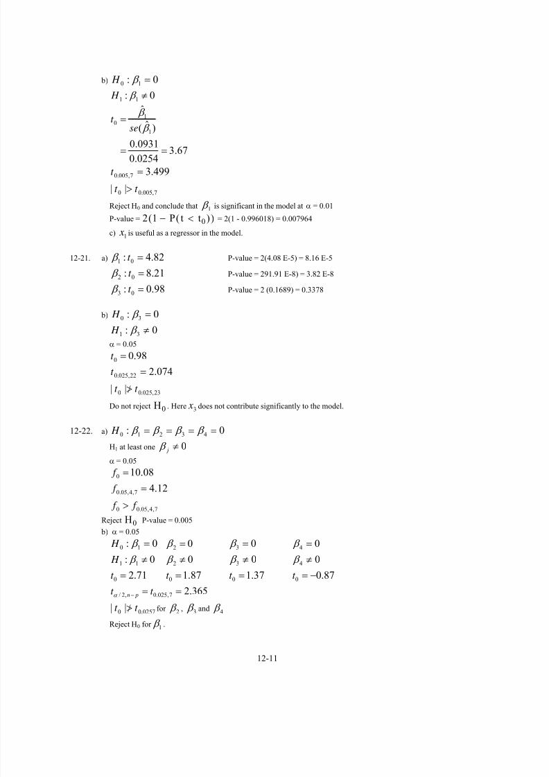
7/12/2019 Solution Manual Stats
http://slidepdf.com/reader/full/solution-manual-stats 386/588
b) 0: 10 = β H
0: 11 ≠ β H
67.30254.0
0931.0
)ˆ(
ˆ
1
10
==
= β
β
set
7,005.00
7,005.0
||
499.3
t t
t
>
=
Reject H0 and conclude that 1 β is significant in the model at α = 0.01
P-value = 2 1 0( (− <P ))t t = 2(1 - 0.996018) = 0.007964
c) 1 x is useful as a regressor in the model.
12-21. a) 82.4: 01 =t β P-value = 2(4.08 E-5) = 8.16 E-5
21.8: 02 =t β P-value = 291.91 E-8) = 3.82 E-8
98.0: 03 =t β P-value = 2 (0.1689) = 0.3378
b) 0: 30 = β H
0: 31 ≠ β H
α = 0.05
98.00 =t
23,025.00
22,025.0
||
074.2
t t
t
>/
=
Do not reject H . Here0 3 x does not contribute significantly to the model.
12-22. a) 0: 43210 ==== β β β β H
H1 at least one 0≠ j β
α = 0.05
7,4,05.00
7,4,05.0
0
12.4
08.10
f f
f
f
>
=
=
Reject H P-value = 0.0050 b) α = 0.05
0: 10 = β H 02 = β 03 = β 04 = β
0: 11 ≠ β H 02 ≠ β 03 ≠ β 04 ≠ β
71.20 =t 87.10 =t 37.10 =t 87.00 −=t
365.27,025.0,2/ ==− t t pnα
0257.00 || t t >/ for 2 β , 3 β and 4 β
Reject H0 for 1 β .
12-11

7/12/2019 Solution Manual Stats
http://slidepdf.com/reader/full/solution-manual-stats 387/588
12-23. a) 0: 6543210 ====== β β β β β β H
H1: at least one 0≠ β
14,6,05.00
14,6,05.014,6,
0
848.2
53.19
f f
f f
f
>
==
=
α
Reject H0 and conclude regression model is significant at α = 0.05
b) The t-test statistics for β1 through β6 are -0.45, -0.07, -3.42, 0.17, -2.90, 0.69. Because t0.025,14=-2.14,
the regressors that contribute to the model at α=0.05 are etw and axle.
12-24. a) 0:0 = j H β for all j
0:1 ≠ j H β for at least one j
14,4,05.00
14,4,05.
0
11.3
16.7
f f
f
f
>
=
=
Reject H0 and conclude regression is significant at α = 0.05. P-value = 0.0023
b) 7792.0ˆ =σ
α = 0.05 t tn pα / , . , .2 025 14 2 145− = =
H 0 2 0:β = β3 0= β4 0= β5 0=
H1 2 0:β ≠ β3 0≠ β4 0≠ β5 0≠
t0 0 113= − . t0 3 83= . t0 1 91= − . t0 0 9= − .
| | / ,t t0 2/> α 14 14 14 | | / ,t t0 2> α | | / ,t t0 2/> α | | / ,t t0 2 14/> α
Do not reject H0 Reject H0 Do not reject H0 Do not reject H0
All variables do not contribute to the model.
12-25. a) 0: 3210 === β β β H
H j1
0:β ≠ for at least one j
16,3,05.00
16,3,05.
0
34.3
828.31
f f
f
f
>
=
=
Reject H0 and conclude regression is significant at α = 0.05
b) 2856.12ˆ 2 =σ
α = 0.05 t tn pα / , . , .2 025 16 2 12− = =
H0 1 0:β = β2 0= β3 0=
H1 1 0:β ≠ β2 0≠ β3 0≠
58.20 −=t 84.10 =t 82.130 =t
16,025.00 || t t > 16,025.00 || t t >/ 16,025.00 || t t >
Reject H0 Do not reject H0 Reject H0
12-26. ARSNAILS = 0.001 + 0.00858 AGE - 0.021 DRINKUSE + 0.010 COOKUSE
Predictor Coef SE Coef T P
Constant 0.0011 0.9067 0.00 0.999
AGE 0.008581 0.007083 1.21 0.242
DRINKUSE -0.0208 0.1018 -0.20 0.841
COOKUSE 0.0097 0.1798 0.05 0.958
12-12

7/12/2019 Solution Manual Stats
http://slidepdf.com/reader/full/solution-manual-stats 388/588
S = 0.506197 R-Sq = 8.1% R-Sq(adj) = 0.0%
Analysis of Variance
Source DF SS MS F P
Regression 3 0.3843 0.1281 0.50 0.687
Residual Error 17 4.3560 0.2562Total 20 4.7403
a)0:
0:
1
3210
≠
===
j H
H
β
β β β
for at least one j; k=4
17,3,05.00
17,3,05.0
0
197.3
50.0
05.0
f f
f
f
<
=
=
=α
Do not reject H0. There is insufficient evidence to conclude that the model is significant at α=0.05. The P-
value =0.687.
b) 0: 10 = β H
0: 11 ≠ β H
α = 0.05
21.1007083.0
008581.0
)ˆ(
ˆ
1
10 ===
β
β
set
11.217,025.0 =t
17,2/0 || α t t < . Fail to reject H , there is not enough evidence to conclude that0 1 β is significant in the
model at α = 0.05.
0: 20 = β H
0: 21 ≠ β H
α = 0.05
2.01018.0
0208.0
)ˆ(
ˆ
2
20 −=
−==
β
β
set
11.217,025.0 =t
17,2/0||
α t t < . Fail to reject H , there is not enough evidence to conclude that
0 2 β is significant in the
model at α = 0.05.
0: 30 = β H
0: 31 ≠ β H
α = 0.05
05.01798.0
0097.0
)ˆ(
ˆ
3
30 ===
β
β
set
12-13

7/12/2019 Solution Manual Stats
http://slidepdf.com/reader/full/solution-manual-stats 389/588
11.217,025.0 =t
17,2/0 || α t t < . Fail to reject H , there is not enough evidence to conclude that0 3 β is significant in the
model at α = 0.05.
12-27. a) 0: 210 == β β H
for at least one:0 H 0≠ j β
α = 0.05
37,2,05.00
37,2,05.0
0
252.3
67.99
f f
f
f
>
=
=
The regression equation israds = - 440 + 19.1 mAmps + 68.1 exposure time
Predictor Coef SE Coef T P
Constant -440.39 94.20 -4.68 0.000
mAmps 19.147 3.460 5.53 0.000
exposure time 68.080 5.241 12.99 0.000
S = 235.718 R-Sq = 84.3% R-Sq(adj) = 83.5%
Analysis of Variance
Source DF SS MS F P
Regression 2 11076473 5538237 99.67 0.000
Residual Error 37 2055837 55563
Total 39 13132310
Reject H0 and conclude regression model is significant at α = 0.05 P-value < 0.000001
b) 55563ˆ 2 == E MSσ
460.3ˆ)ˆ( 2
1 == jjcse σ β
0: 10 = β H
0: 11 ≠ β H
α = 0.05
539.5460.3
147.19
)ˆ(
ˆ
1
10
==
= β
β
set
0262.237,025.0340,025.0 ==− t t
37,2/0 || α t t > , Reject H and conclude that0 1 β is significant in the model at α = 0.05
241.5ˆ)ˆ( 2
2 == jjcse σ β
0: 20 = β H
12-14

7/12/2019 Solution Manual Stats
http://slidepdf.com/reader/full/solution-manual-stats 390/588
0: 21 ≠ β H
α = 0.05
99.12241.5080.68
)ˆ(
ˆ
2
20
==
= β
β
set
0262.237,025.0340,025.0 ==− t t
37,2/0 || α t t > , Reject H conclude that0 2 β is significant in the model at α = 0.05
12-28.The regression equation is
y = - 171 + 7.03 x1 + 12.7 x2
Predictor Coef SE Coef T P
Constant -171.26 28.40 -6.03 0.001
x1 7.029 1.539 4.57 0.004
x2 12.696 1.539 8.25 0.000
S = 3.07827 R-Sq = 93.7% R-Sq(adj) = 91.6%
Analysis of Variance
Source DF SS MS F P
Regression 2 842.37 421.18 44.45 0.000
Residual Error 6 56.85 9.48
Total 8 899.22
a) 0: 210 == β β H
for at least one:1 H 0≠ j β
α = 0.05
6,2,05.00
6,2,05.0
0
14.5
45.446/85.56
2/37.842
f f
f
f
pn
SS
k
SS
E
R
>
=
===−
Reject H0 and conclude regression model is significant at α = 0.05 P-value ≈ 0
b) 48.9ˆ 2 == E MSσ
539.1ˆ)ˆ( 21 == jjcse σ β
0: 10 = β H
0: 11 ≠ β H
α = 0.05
12-15

7/12/2019 Solution Manual Stats
http://slidepdf.com/reader/full/solution-manual-stats 391/588
568.4539.1
03.7
)ˆ(
ˆ
1
10
==
= β
β
set
447.26,025.039,025.0 ==− t t
6,2/0 || α t t > , Reject H ,0 1 β is significant in the model at α = 0.05
539.1ˆ)ˆ( 2
2 == jjcse σ β
0: 20 = β H
0: 21 ≠ β H
α = 0.05
252.8539.1
7.12
)ˆ(
ˆ
2
20
==
= β
β
set
447.26,025.039,025.0 ==− t t
6,2/0 || α t t > , Reject H conclude that0 2 β is significant in the model at α = 0.05
c) With a smaller sample size, the difference in the estimate from the hypothesized value needs to be
greater to be significant.
12-29.Useful range (ng) = 239 + 0.334 Brightness (%) - 2.72 Contrast (%)
Predictor Coef SE Coef T PConstant 238.56 45.23 5.27 0.002
Brightness (%) 0.3339 0.6763 0.49 0.639
Contrast (%) -2.7167 0.6887 -3.94 0.008
S = 36.3493 R-Sq = 75.6% R-Sq(adj) = 67.4%
Analysis of Variance
Source DF SS MS F P
Regression 2 24518 12259 9.28 0.015
Residual Error 6 7928 1321
Total 8 32446
a) 0: 210 == β β H
for at least one:1 H 0≠ j β
α = 0.05
12-16

7/12/2019 Solution Manual Stats
http://slidepdf.com/reader/full/solution-manual-stats 392/588
6,2,05.00
6,2,05.0
0
14.5
28.96/7928
2/24518
f f
f
f pn
SS
k
SS
E
R
>
=
===−
Reject H0 and conclude that the regression model is significant at α = 0.05 P-value =0.015
b) 1321ˆ 2 == E MSσ
6763.0ˆ)ˆ( 2
1 == jjcse σ β
0: 10 = β H
0: 11 ≠ β H
α = 0.05
49.06763.0
3339.0
)ˆ(
ˆ
1
10
==
=
β
β
set
447.26,025.039,025.0 ==− t t
6,2/0 || α t t < , Fail to reject H , there is no enough evidence to conclude that0 1 β is significant in the model at α =
0.05
6887.0ˆ)ˆ( 2
2 == jjcse σ β
0: 20 = β H
0: 21 ≠ β H
α = 0.05
94.36887.0
7167.2
)ˆ(
ˆ
2
20
−=−
=
= β
β
set
447.26,025.039,025.0 ==− t t
6,2/0 || α t t > , Reject H conclude that0 2 β is significant in the model at α = 0.05
12-30.The regression equation is
Stack Loss(y) = - 39.9 + 0.716 X1 + 1.30 X2 - 0.152 X3
Predictor Coef SE Coef T P
Constant -39.92 11.90 -3.36 0.004
X1 0.7156 0.1349 5.31 0.000
X2 1.2953 0.3680 3.52 0.003
X3 -0.1521 0.1563 -0.97 0.344
S = 3.24336 R-Sq = 91.4% R-Sq(adj) = 89.8%
12-17

7/12/2019 Solution Manual Stats
http://slidepdf.com/reader/full/solution-manual-stats 393/588
Analysis of Variance
Source DF SS MS F P
Regression 3 1890.41 630.14 59.90 0.000
Residual Error 17 178.83 10.52
Total 20 2069.24
a)
0: 3210 === β β β H
0:1 ≠ j H β for at least one j
α = 0.05
17,3,05.00
17,3,05.0
0
20.3
90.5917/83.178
3/41.189
f f
f
f pn
SS
k
SS
E
R
>
=
===−
Reject H0 and conclude that the regression model is significant at α = 0.05 P-value < 0.000001
b) 52.10ˆ 2 == E MSσ
1349.0ˆ)ˆ( 2
1 == jjcse σ β
0: 10 = β H
0: 11 ≠ β H
α = 0.05
31.51349.0
7156.0
)ˆ(
ˆ
1
10
==
= β
β
set
110.217,025.0421,025.0 ==− t t
17,2/0 || α t t > . Reject H and conclude that0 1 β is significant in the model at α = 0.05.
3680.0ˆ)ˆ( 2
2 == jjcse σ β
0: 20 = β H
0: 21 ≠ β H
α = 0.05
52.33680.0
2953.1
)ˆ(
ˆ
2
2
0
==
= β
β
set
110.217,025.0421,025.0 ==− t t
17,2/0 || α t t > . Reject H and conclude that0 2 β is significant in the model at α = 0.05.
12-18

7/12/2019 Solution Manual Stats
http://slidepdf.com/reader/full/solution-manual-stats 394/588
1563.0ˆ)ˆ( 2
3 == jjcse σ β
0: 30 = β H
0: 31 ≠ β H
α = 0.05
97.01563.0
1521.0
)ˆ(
ˆ
3
30
−=−
=
= β
β
set
110.217,025.0421,025.0 ==− t t
17,2/0 || α t t < . Fail to reject H , there is not enough evidence to conclude that0 3 β is significant in the model at α =
0.05.
12-31.
Rating Pts = 3.22 + 1.22 Pct Comp + 4.42 Pct TD - 4.09 Pct Int
Predictor Coef SE Coef T P
Constant 3.220 6.519 0.49 0.626
Pct Comp 1.2243 0.1080 11.33 0.000
Pct TD 4.4231 0.2799 15.80 0.000
Pct Int -4.0914 0.4953 -8.26 0.000
S = 1.92094 R-Sq = 97.8% R-Sq(adj) = 97.5%
Analysis of Variance
Source DF SS MS F P
Regression 3 4196.3 1398.8 379.07 0.000
Residual Error 26 95.9 3.7Total 29 4292.2
a) 0: 10730 === β β β H
0:1 ≠ j H β for at least one j
α = 0.05
26,3,05.00
26,3,05.
0
98.2
07.379
f f
f
f
>>
=
=
Reject H0
and conclude that the regression model is significant at α = 0.05 P-value
≈0
b) All at α = 0.05 056.226,025. =t
0: 30 = β H 0: 70 = β H 0: 100= β H
H1 3 0:β ≠ 0: 71 ≠ β H 0: 101 ≠ β H
33.110 =t 80.150 =t 26.80 −=t
26,2/0 || α t t > 26,2/0 || α t t > 26,2/0 || α t t >
Reject H0 Reject H0 Reject H0
12-19

7/12/2019 Solution Manual Stats
http://slidepdf.com/reader/full/solution-manual-stats 395/588
c)
The regression equation is
Rating Pts = - 33.6 + 2.18 Pct Comp - 4.54 Pct Int
Predictor Coef SE Coef T P
Constant -33.60 19.46 -1.73 0.096
Pct Comp 2.1842 0.2855 7.65 0.000Pct Int -4.540 1.580 -2.87 0.008
S = 6.13862 R-Sq = 76.3% R-Sq(adj) = 74.5%
Analysis of Variance
Source DF SS MS F P
Regression 2 3274.8 1637.4 43.45 0.000
Residual Error 27 1017.4 37.7
Total 29 4292.2
SSR (full model) = 4196.3 SSR (reduced model) = 3274.8
Difference = 4196.3 – 3274.8 =921.5α = 0.05
24,1,05.00
26,1,05.0
0
26.4
1.2497.3
5.9211/9.2558
f f
f
MS f
E
>>
=
===
Reject H0 and conclude that the TD percentage regressor is significant at α = 0.05
P-value 0≈ Note that f 0 = 691.6 = t-statistic
2= 15.80
2= 249.6 (except for rounding error)
12-32. a) H j0 0:β = for all j
H j1 0:β ≠for at least one j
26,5,0
26,5,05.
0
59.2
9902.158
α f f
f
f
>
=
=
Reject H0 and conclude regression is significant at α = 0.05
P-value < 0.000001
b) α = 0.05 t tn pα / , . , .2 025 26 2 056− = =
0: 10= β H 02 = β 03 = β 04 = β 05 = β
0: 11 ≠ β H 02 ≠ β 03 ≠ β 04 ≠ β 05 ≠ β
83.00 =t 25.120 =t 52.0
0 −=t 96.60 =t 29.00 −=t
Do not Reject H0 Reject H0 Do not reject H0 Reject H0 Do not reject H0
c) 21 009325.0002687.0010889.0ˆ x x y ++=
d) H j0 0:β = for all j
H j1 0:β ≠ for at least one j
29,2,05.00
29,2,05.
0
33.3
455.308
f f
f
f
>
=
=
Reject H0 and conclude regression is significant at α = 0.05
12-20

7/12/2019 Solution Manual Stats
http://slidepdf.com/reader/full/solution-manual-stats 396/588
α = 0.05 045.229,025.,2/ ==− t t pnα
0: 10= β H 02 = β
0: 11 ≠ β H 02 ≠ β
31.180 =t 37.60 =t
| | / ,t t0 2 2> α 9 | | / ,t t0 2> α 29
Reject H0 for each regressor variable and conclude that both variables are significant at α = 0.05
e) 67.6ˆ)( −= E d part σ . Part c) is smaller, suggesting a better model.
12-33. , Assume no interaction model.22110ˆˆˆˆ x x y β β β ++=
a) 0: 210 == β β H
H1 at least one 0≠ j β
3,2,05.00
3,2,05.0
0
55.9
59.97
f f
f
f
>
=
=
Reject H0 P-value = 0.002
b) 0: 10= β H 0: 20
= β H
0: 11 ≠ β H 0: 21 ≠ β H
42.60 −=t 57.20 −=t
182.33,025.03,2/ == t t α 182.33,025.03,2/ == t t α
3,025.00 || t t > 3,025.00 || t t >/
Reject H0 for regressor 1 β . Do not reject H0 for regressor 2 β .
c) 1012),|( 012 = β β β RSS
0: 20 = β H
0: 21 ≠ β H
α = 0.05
3,1,05.00
3,1,05.3,1,
0
13.10
629.6
f f
f f
f
>/
==
=
α
Do not reject H0
d) 0:12210
=== β β β H
H 1 at least one 0≠ j β
α = 0.05
2,3,05.00
2,3,05.02,3,
0
16.19
714.7
f f
f f
f
>/
==
=
α
Do not reject H0
12-21

7/12/2019 Solution Manual Stats
http://slidepdf.com/reader/full/solution-manual-stats 397/588
e) 0: 120 = β H
0: 121 ≠ β H
α = 0.05
2,1,05.00
2,1,05.0
0
2112
51.18
11.1147
9.163
9.163297874.29951),|(
f f
f
MSSSR f
SSR
E
>/
=
===
=−= β β β
Do not reject H0
f) 0.147ˆ 2 =σ
σ2 (no interaction term) = 153.0
)ˆ( 2σ E MS was reduced in the model with the interaction term.
12-34. a) 0:0 = j H β for all j
0:1 ≠ j H β for at least one j
15,14,05.00
15,14,05.
0
424.2
77.9
f f
f
f
>
=
=
Reject H0 and conclude that the regression model is significant at α = 0.05
b) 0:0 = j H β
0:1 ≠ j H β
131.215,025. =t
GF : Reject H32.20 =t 0
GA : Reject H58.30 −=t 0
ADV : Do not reject H61.00 =t 0
PPGF : Do not reject H60.00 −=t 0
PCTG : Do not reject H70.00 =t 0
PEN : Do not reject H70.00 =t 0
BMI : Do not reject H03.00 =t 0
AVG : Do not reject H67.00 −=t 0
SHT : Do not reject H02.10 −=t 0
PPGA : Do not reject H25.00
=t 0
PKPCT : Do not reject H07.00 =t 0
SHGF : Do not reject H48.10 =t 0
SHGA : Do not reject H38.10 =t 0
FG : Do not reject H71.00 =t 0
No, only "GF" (β1 ) and “GA” (β2 ) are significant at α = 0.05
c)
12-22

7/12/2019 Solution Manual Stats
http://slidepdf.com/reader/full/solution-manual-stats 398/588
35.3
10.19
1075.028108.071.17ˆ
27,2,05.
0
41
=
=
−+−=
f
f
x x y
Reject H0
0: 10 = β H 04 = β
0: 11 ≠ β H 04 ≠ β
70.50=t 86.00
−=t
Reject H0 Do not reject H0
Based on the t-test, power play goals for (PPGF) is not a logical choice to add to the model that already contains the
number of goals for.

7/12/2019 Solution Manual Stats
http://slidepdf.com/reader/full/solution-manual-stats 399/588
Sections 12-3 and 12-4
12-35. a)00
2
,2/0ˆˆ ct pnσ β α −±
183.292927.49
128.121055.171
)217.51)(365.2(055.171
)ˆ(055.171
0
07,025.
≤≤
±
±
±
β
β set
11
2
,2/1ˆˆ ct pn σ β α −±
393.7033.0
680.3713.3
)556.1)(365.2(713.3
)ˆ(713.3
1
17,025.
≤≤
±
±
±
β
β set
22
2
,2/2ˆˆ ct
pnσ β α −±
513.0765.2
639.1126.1
)693.0)(365.2(126.1
)ˆ(126.1
2
07,025.
≤≤−
±−
±−
±−
β
β set
b) 181 = x
471.189ˆ
43
0
2
=
=
y
x
127.220815.158
)305065.0(7875.550)365.2(471.189
305065.0)'(
0|
0
1'
0
≤≤
±
=−
xY
X X X X
μ
c) α = 0.05
181 = x
471.189ˆ43
0
2
==
y x
12-23

7/12/2019 Solution Manual Stats
http://slidepdf.com/reader/full/solution-manual-stats 400/588
878.252064.126
)305065.1(7875.550)365.2(471.189
))'(1(ˆˆ
305065.0)'(
0
0
1'
0
2
,2/
0
1'
0
≤≤
±
+±
=
−
−
−
y
X X X X t y
X X X X
pn σ α
12-36.a)00
2,2/0 ˆˆ ct pn σ β α −±
8678.216922.25
78.239122.1
)055.10)(365.2(9122.1
)ˆ(9122.1
0
07,025.
≤≤−
±−
±−
±−
β
β set
11
2
,2/1ˆˆ ct pnσ β α −
±
2887.01025.0
1956.00931.0
)0827.0)(365.2(0931.0
)ˆ(0931.0
1
17,025.
≤≤−
±
±
±
β
β set
22
2
,2/2ˆˆ ct pn σ β α −±
7257.02193.0
4725.02532.0
)1998.0)(365.2(2532.0
)ˆ(2532.0
2
07,025.
≤≤−
±
±
±
β
β set
b) x 1 200=
37.29ˆ50
0
2
==
y x
429.39311.19
059.1037.29
)211088.0(694.85)365.2(37.29
211088.0)'(
0|
0
1'
0
≤≤
±
±
=−
xY
X X X X
μ
c) α = 0.05
x 1 200=
37.29ˆ
50
0
2
=
=
y
x
463.53277.5
093.2437.29
)211088.1(694.85)365.2(37.29
))'(1(ˆˆ
211088.0)'(
0
0
1'
0
2
,2/
0
1'
0
≤≤
±
±
+±
=
−
−
−
y
X X X X t y
X X X X
pn σ α
12-37. a) 269.1477.20 1 ≤≤− β
12-24

7/12/2019 Solution Manual Stats
http://slidepdf.com/reader/full/solution-manual-stats 401/588
159.22428.14
076.1245.0
3
2
≤≤
≤≤−
β
β
b) 91.372ˆ0| = xY μ 721.4)ˆ( 0 = yse 921.216,005. =t
162.105582.77
)721.4(921.2372.91
0 ≤≤
±
yc) 91.372ˆ
0| = xY μ 3.163)ˆ(0| = xY se μ
611.100133.82
)163.3)(921.2(372.91
0| ≤≤
±
xY μ
12.38. a) 95 % CI on coefficients
4172.10973.0 1 ≤≤ β
8319.07941.1
7613.67953.1
0026.179646.1
4
3
2
≤≤−
≤≤−
≤≤−
β
β
β
b) 44.290ˆ0| = xY
μ 61.7)ˆ(0| = xY se μ 365.27,025. =t
44.30844.272
)61.7)(365.2(44.290
)ˆ(ˆ
0
00
|
|,2/|
≤≤
±
± −
xY
xY pn xY set
μ
μ μ α
c) ))(1(ˆˆ0
1
0
2
,2/0 xXXx−
−′
′+± σ α pnt y
64.32325.257
)038.14(365.244.290
0
≤≤
±
y
12-39. a) 3295.09467.6 1 −≤≤− β
1417.03651.0 2 ≤≤− β
b) 5156.308276.45 1 ≤≤− β
04251.003433.0
8984.03426.1
12
2
≤≤−
≤≤−
β
β
These part b. intervals are much wider.
Yes, the addition of this term increased the standard error of the regression coefficient estimators.
12-40. a) 535.0595.0 2 ≤≤− β
9756.22968.7
013.0216.0
812.0229.0
5
4
3
≤≤−
≤≤−
≤≤
β
β
β
b) .|μY x08 99568= se Y x( ) .|μ
00 472445= t. , .025 14 2 145=
12-25
7/12/2019 Solution Manual Stats
http://slidepdf.com/reader/full/solution-manual-stats 402/588
009.10982.7
)472445.0)(145.2(99568.8
)ˆ(ˆ
0
00
|
|,2/|
≤≤
±
± −
xY
xY pn xY set
μ
μ μ α
c) .y0 8 99568= se y( ) .0 100121=
143.118481.6
)00121.1(145.299568.8
0 ≤≤± y
12-41. a)
11
2
,2/1ˆˆ ct pn σ β α −±
1577.261363.12
014458.7147.19
)460.3)(0262.2(147.19
)ˆ(147.19
1
137,025.
≤≤
±
±
±
β
β set
22
2,2/2
ˆˆ ct pn σ β α −±
6993.784607.57
014458.7080.68
)241.5)(0262.2(080.68
)ˆ(080.68
2
237,025.
≤≤
±
±
±
β
β set
b)
1.85ˆ0| −= xY
μ 6.54)ˆ(0| = xY se μ 7154.237,005.0 =t
2.634.233)6.54)(7154.2(1.85
)ˆ(ˆ
0
00
|
|,2/|
≤≤−
±−
± −
xY
xY pn xY set
μ
μ μ α
c) 1.85ˆ0 −= y 95.241)ˆ( 0 = yse
89.57109.742
)95.241(7154.21.85
0 ≤≤−
±−
y
12-42.The regression equation isARSNAILS = 0.001 + 0.00858 AGE - 0.021 DRINKUSE + 0.010 COOKUSE
Predictor Coef SE Coef T PConstant 0.0011 0.9067 0.00 0.999AGE 0.008581 0.007083 1.21 0.242DRINKUSE -0.0208 0.1018 -0.20 0.841COOKUSE 0.0097 0.1798 0.05 0.958
S = 0.506197 R-Sq = 8.1% R-Sq(adj) = 0.0%
Analysis of Variance
12-26

7/12/2019 Solution Manual Stats
http://slidepdf.com/reader/full/solution-manual-stats 403/588
Source DF SS MS F PRegression 3 0.3843 0.1281 0.50 0.687Residual Error 17 4.3560 0.2562Total 20 4.7403
a) 898.217,005.0 =t
531.0511.0
274.0316.0
0291.0012.0
634.2617.2
3
2
1
0
≤≤−
≤≤−
≤≤−
≤≤−
β
β
β
β
b)
214.0ˆ 0| = xY μ 216.0)ˆ( 0| = xY se μ 898.216,005.0 =t
840.0412.0
)216.0)(898.2(214.0
)ˆ(ˆ
0
00
|
|,2/|
≤≤−
±
± −
xY
xY pn xY set
μ
μ μ α
c) 214.0ˆ0 = y 5503.0)ˆ( 0 = yse
809.1381.1
)5503.0(898.2214.0
0 ≤≤−
±
y
12-43. a) 860.18,05.0 =t
-0.576 ≤ β0 ≤ 0.355
959.12743.8
7201.00943.0
2
1
≤≤−
≤≤
β
β
b)
8787.0ˆ0| = xY
μ 00926.0)ˆ(0| = xY se μ 860.116,005.0 =t
89592.086148.0
)00926.0)(860.1(8787.0
)ˆ(ˆ
0
00
|
|,2/|
≤≤
±
± −
xY
xY pn xY set
μ
μ μ α
c) 8787.0ˆ0 = y 0134.0)ˆ( 0 = yse
90250.085490.0
)0134.0(86.18787.0
0 ≤≤
±
y
12-44.The regression equation is
12-27

7/12/2019 Solution Manual Stats
http://slidepdf.com/reader/full/solution-manual-stats 404/588
y = - 171 + 7.03 x1 + 12.7 x2
Predictor Coef SE Coef T PConstant -171.26 28.40 -6.03 0.001x1 7.029 1.539 4.57 0.004x2 12.696 1.539 8.25 0.000
S = 3.07827 R-Sq = 93.7% R-Sq(adj) = 91.6%
Analysis of Variance
Source DF SS MS F PRegression 2 842.37 421.18 44.45 0.000Residual Error 6 56.85 9.48Total 8 899.22
a)
11
2
,2/1ˆˆ ct
pnσ β α −
±
796.10264.3
766.303.7
)539.1)(447.2(03.7
)ˆ(03.7
1
16,025.
≤≤
±
±
±
β
β set
22
2
,2/2ˆˆ ct
pnσ β α −
±
466.16934.8
766.37.12
)539.1)(447.2(7.12
)ˆ(7.12
1
26,025.
≤≤
±
±
±
β
β set
b)
NewObs Fit SE Fit 95% CI 95% PI
1 140.82 6.65 (124.54, 157.11) (122.88, 158.77)XX
82.140ˆ0| =
xY μ 65.6)ˆ(
0| = xY se μ 447.26,025.0 =t
09.15755.124
)65.6)(447.2(82.140
)ˆ(ˆ
0
00
|
|,2/|
≤≤
±
± −
xY
xY pn xY set
μ
μ μ α
c) 82.140ˆ0 = y 33.7)ˆ( 0 = yse
76.15888.122
)33.7(447.282.140
0 ≤≤
±
y
12-28

7/12/2019 Solution Manual Stats
http://slidepdf.com/reader/full/solution-manual-stats 405/588
d) The smaller the sample size, the wider the interval
12-45.
The regression equation isUseful range (ng) = 239 + 0.334 Brightness (%) - 2.72 Contrast (%)
Predictor Coef SE Coef T PConstant 238.56 45.23 5.27 0.002Brightness (%) 0.3339 0.6763 0.49 0.639Contrast (%) -2.7167 0.6887 -3.94 0.008
S = 36.3493 R-Sq = 75.6% R-Sq(adj) = 67.4%
Analysis of Variance
Source DF SS MS F PRegression 2 24518 12259 9.28 0.015Residual Error 6 7928 1321
Total 8 32446
a) 707.36,005.0 =t
164.0270.5
841.2173.2
2
1
−≤≤−
≤≤−
β
β
b)Predicted Values for New Observations
NewObs Fit SE Fit 99% CI 99% PI
1 44.6 21.9 (-36.7, 125.8) (-112.8, 202.0)
Values of Predictors for New Observations
New ContrastObs Brightness (%) (%)
1 70.0 80.0
6.44ˆ0| =
xY μ 9.21)ˆ(
0| = xY se μ 707.36,005.0 =t
8.1257.36
)9.21)(707.3(6.44
)ˆ(ˆ
0
00
|
|,2/|
≤≤−
±
± −
xY
xY pn xY set
μ
μ μ α
c) 6.44ˆ0 = y 44.42)ˆ( 0 = yse
0.2028.112
)44.42(707.36.44
0 ≤≤−
±
y
d) Predicted Values for New Observations
NewObs Fit SE Fit 99% CI 99% PI
1 187.3 21.6 (107.4, 267.2) (30.7, 344.0)
12-29

7/12/2019 Solution Manual Stats
http://slidepdf.com/reader/full/solution-manual-stats 406/588
Values of Predictors for New Observations
New ContrastObs Brightness (%) (%)
1 50.0 25.0
CI: 2.2674.1070| ≤≤ xY μ
PI: 0.3447.30 0 ≤≤ y
These intervals are wider because the regressors are set at extreme values in the x space and the standard
errors are greater.
12-46. a) 110.217,025.0 =t
178.0482.0
072.2519.0
00.1431.0
3
2
1
≤≤−
≤≤
≤≤−
β
β
β
b) 023.36ˆ0| =
xY μ 803.1)ˆ(
0| = xY se μ 110.217,025.0 =t
827.39219.32
)803.1)(110.2(023.36
)ˆ(ˆ
0
00
|
|,2/|
≤≤
±
± −
xY
xY pn xY set
μ
μ μ α
c) 023.36ˆ0 = y 698.3)ˆ( 0 = yse
852.43194.28
)698.3(110.2023.36
0 ≤≤
±
y
d) Prediction at x1 = 80, x2 = 19, x3 = 93 is 795.270| = xY μ
CI: 559.34030.210| ≤≤ xY μ
PI: 417.37173.18 0 ≤≤ y
12-47. a) 056.226,025.0 =t
073.3110.5
999.4848.3
446.1002.1
623.16183.10
10
7
3
0
−≤≤−
≤≤
≤≤
≤≤−
β
β
β
β
b) )ˆ(3877.0)'(ˆ0|0
1'
0
2
xY se X X X X μ σ ==−
c) 079.82)3(091.4)4(423.4)60(224.122.3ˆ =−++= y
876.82282.81
7971.0079.82
)3877.0)(056.2(079.82
)ˆ(ˆ
0
00
|
|24,025.|
≤≤
±
±
±
xY
xY xY set
μ
μ μ
12-48. a) 000099.0000042.0 1 ≤≤− β
12-30

7/12/2019 Solution Manual Stats
http://slidepdf.com/reader/full/solution-manual-stats 407/588
01424.001897.0
010979.000597.0
00898.001504.0
00268.000196.0
5
4
3
2
≤≤−
≤≤
≤≤−
≤≤
β
β
β
β
b) 022466.0ˆ 0| = xY μ 000595.0)ˆ( 0| = xY se μ 056.226,025. =t
0237.00212.0
)000595.0)(056.2(0220086.0
0| ≤≤
±
xY μ
c) 0171.0ˆ0| = xY μ 000548.0)ˆ(
0| = xY se μ 045.229,025. =t
0183.00159.0
)000548.0)(045.2(0171.0
0| ≤≤
±
xY μ
d) : width = 2.2 E-3
: width = 2.4 E-3
The interaction model has a shorter confidence interval. Yes, this suggests the interaction model is preferable.
12-49. a) t.005,14=2.977
523.0102.1
101.0811.7
546.5962.4
0006.0
047.005.0
059.008.0
458.108658.8
10
9
8
7
3
2
0
−≤≤
≤≤−
≤≤−
≤≤−
≤≤−
≤≤−
≤≤−
β
β
β
β
β
β
β
b)71.29ˆ 0| = xY μ
395.1)ˆ( 0| = xY se μ
863.33557.25
)395.1)(977.2(71.29
)ˆ(ˆ
0
00
|
|14,005.|
≤≤
±
±
xY
xY xY set
μ
μ μ
c) 972 457.30035.00208.0001.61ˆ x x x y −−−=
429.0485.6001.0006.0
006.0036.0
147.71855.50
898.2
9
7
2
0
17,005.
−≤≤−−≤≤−
−≤≤−
≤≤
=
β β
β
β
t
d) The intervals in part c) are narrower. All of the regressors used in part c) are significant, but not all of
those used in part a) are significant. The model used in part c) is preferable.
12-50. a) 2369.00102.0 1 ≤≤ β
b)125956.0329.19ˆ x y +−=
12-31

7/12/2019 Solution Manual Stats
http://slidepdf.com/reader/full/solution-manual-stats 408/588
c) 3456.01735.0 1 ≤≤ β
d) The simple linear regression model has the shorter interval. Obviously there are extraneous variables in
the model from part a), but there are two good predictors in that model, only one of which is included in
the model of part b). Still the shorter interval is an initial indicator that the original model with all variables
might be improved.

7/12/2019 Solution Manual Stats
http://slidepdf.com/reader/full/solution-manual-stats 409/588
Section 12-5
12-51.
a)The regression equation ismpg = 49.9 - 0.0104 cid - 0.0012 rhp - 0.00324 etw + 0.29 cmp - 3.86 axle
+ 0.190 n/v
Predictor Coef SE Coef T PConstant 49.90 19.67 2.54 0.024cid -0.01045 0.02338 -0.45 0.662rhp -0.00120 0.01631 -0.07 0.942
etw -0.0032364 0.0009459 -3.42 0.004cmp 0.292 1.765 0.17 0.871axle -3.855 1.329 -2.90 0.012n/v 0.1897 0.2730 0.69 0.498
S = 2.22830 R-Sq = 89.3% R-Sq(adj) = 84.8%
b) There appears to be an outlier. Otherwise, the normality assumption is not violated.
Standardized Residual
S c o r e
3210-1-2-3
2
1
0
-1
-2
Norma l Pr obab i li t y P lo t o f the Res iduals(response is mpg)
c) The plots do not show any violations of the assumptions.
12-32

7/12/2019 Solution Manual Stats
http://slidepdf.com/reader/full/solution-manual-stats 410/588
Fitted Value
S t a n d a r d
i z e d
R e s i d u a l
4035302520
2
1
0
-1
-2
-3
Residuals Versus the Fi t ted Values(response is mpg)
cid
S t a n d a r d i z e d
R e s i d u a l
500400300200100
2
1
0
-1
-2
-3
Residuals Versus cid(response is mpg)
et w
S
t a n d a r d i z e d
R e s i d u a l
6000550050004500400035003000
2
1
0
-1
-2
-3
Residuals Versus etw(response is mpg)
cmp
S t a n d a r d i z e d
R e s i d u a l
10.009.759.509.259.008.758.50
2
1
0
-1
-2
-3
Residuals Ver sus cmp(response is mpg)
12-33

7/12/2019 Solution Manual Stats
http://slidepdf.com/reader/full/solution-manual-stats 411/588
axle
S t a n d a r d
i z e d
R e s i d u a l
4.254.003.753.503.253.002.752.50
2
1
0
-1
-2
-3
Residuals Versus axle(response is mpg)
n/ v
S t a n d a r d i z e d
R e s i d u a l
4035302520
2
1
0
-1
-2
-3
Residuals Versus n/ v(response is mpg)
d)
0.036216, 0.000627, 0.041684, 0.008518, 0.026788, 0.040384, 0.003136,
0.196794, 0.267746, 0.000659, 0.075126, 0.000690, 0.041624, 0.070352,
0.008565, 0.051335, 0.001813, 0.019352, 0.000812, 0.098405, 0.574353
None of the values is greater than 1 so none of the observations are influential.
12-52. a)2 = R 852.0
b) The residual plots look reasonable. There is some increase in variability at the middle of the predicted
values.
c) Normality assumption is reasonable. The residual plots appear reasonable too.
Residual
P e r c e n t
20100-10-20
99
95
90
80
70
60
50
40
30
20
10
5
1
Normal Probability Plot of the Residuals(response is y)
12-34

7/12/2019 Solution Manual Stats
http://slidepdf.com/reader/full/solution-manual-stats 412/588
x1
R
e s i d u a l
9080706050403020
10
5
0
-5
-10
-15
Residuals Versus x1(response is y)
x2
R
e s i d u a l
262524232221
10
5
0
-5
-10
-15
Residuals Versus x2(response is y)
x3
R
e s i d u a l
94939291908988878685
10
5
0
-5
-10
-15
Residuals Versus x3(response is y)
x4
R
e s i d u a l
1101051009590
10
5
0
-5
-10
-15
Residuals Versus x4(response is y)
12-53. a) %8.972 = R b) Assumption of normality appears adequate.
Residual
P e r c e n t
543210-1-2-3-4
99
95
90
80
70
60
50
40
30
20
10
5
1
Normal Probability Plot of the Residuals(response is Rating Pts)
c) Model appears adequate. Some suggestion of nonconstant variance in the plot of x (percentage of TDs)7
Fitt ed Value
R e s i d u a l
120110100908070
4
3
2
1
0
-1
-2
-3
-4
-5
Residuals Versus the Fitted Values(response is Rating Pts)
Pct Comp
R e s i d u a l
70.067.565.062.560.057.555.0
4
3
2
1
0
-1
-2
-3
-4
-5
Residuals Versus Pct Comp(response is Rating Pts)
12-35
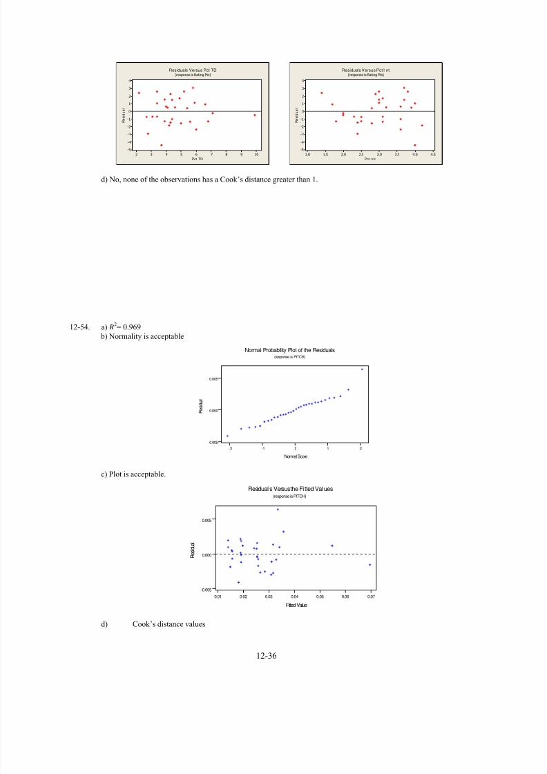
7/12/2019 Solution Manual Stats
http://slidepdf.com/reader/full/solution-manual-stats 413/588
Pct TD
R e s i d u a l
1098765432
4
3
2
1
0
-1
-2
-3
-4
-5
Residuals Versus Pct TD(response is Rating Pts)
Pct Int
R e s i d u a l
4.54.03.53.02.52.01.51.0
4
3
2
1
0
-1
-2
-3
-4
-5
Residuals Versus Pct I nt(response is Rating Pts)
d) No, none of the observations has a Cook’s distance greater than 1.
12-54. a) R2= 0.969
b) Normality is acceptable
210-1-2
0.005
0.000
-0.005
Normal Score
R e s i d u a l
Normal Probability Plot of the Residuals(response is PITCH)
c) Plot is acceptable.
0.070.060.050.040.030.020.01
0.005
0.000
-0.005
Fitted Value
R e s i d u a l
Residual s Versus the Fitted Values(response is PITCH)
d) Cook’s distance values
12-36

7/12/2019 Solution Manual Stats
http://slidepdf.com/reader/full/solution-manual-stats 414/588
0.0191 0.0003 0.0026 0.0009 0.0293 0.1112 0.1014 0.0131 0.0076 0.0004 0.0109
0.0000 0.0140 0.0039 0.0002 0.0003 0.0079 0.0022 4.5975 0.0033 0.0058 0.1412
0.0161 0.0268 0.0609 0.0016 0.0029 0.3391 0.3918 0.0134 0.0088 0.5063
The 19th observation is influential
12-55. a) %3.842 = R
b) Assumption of normality appears adequate.
Residual
P e r c e n t
7505002500-250-500
99
95
90
80
70
60
50
40
30
20
10
5
1
Normal Probability Plot of the Residuals(response is rads)
c) There are funnel shapes in the graphs, so the assumption of constant variance is violated. The model is
inadequate.
Fitt ed Value
R e s i d u a l
150010005000-500
750
500
250
0
-250
-500
Residuals Versus the Fitted Values(response is rads)
exposure time
R e s i d u a l
20151050
750
500
250
0
-250
-500
Residuals Versus exposure time(response is rads)
mAmps
R e s i d u a l
40353025201510
750
500
250
0
-250
-500
Residuals Versus mAmps(response is rads)
d) Cook’s distance values
12-37

7/12/2019 Solution Manual Stats
http://slidepdf.com/reader/full/solution-manual-stats 415/588
0.032728 0.029489 0.023724 0.014663 0.008279 0.008611
0.077299 0.3436 0.008489 0.007592 0.006018 0.003612
0.001985 0.002068 0.021386 0.105059 0.000926 0.000823
0.000643 0.000375 0.0002 0.000209 0.002467 0.013062
0.006095 0.005442 0.0043 0.002564 0.0014 0.001459
0.015557 0.077846 0.07828 0.070853 0.057512 0.036157
0.020725 0.021539 0.177299 0.731526 No, none of the observations has a Cook’s distance greater than 1.
12-56. a) %1.82 = R
b) Assumption of normality appears is not adequate.
Residual
P e r c e n t
1.51.00.50.0-0.5-1.0
99
95
90
80
70
60
50
40
30
20
10
5
1
Normal Probabilit y Plot of the Residuals(response is ARSNAILS)
c) The graphs indicate non-constant variance. Therefore, the model is not adequate.
Fitted Value
S t a n d a r d i z e d
R e s i d
u a l
0.70.60.50.40.30.20.10.0
4
3
2
1
0
-1
Residuals Versus the Fi t t ed Values(response is ARSNAILS)
AGE
R e s i d u a l
9080706050403020100
1.5
1.0
0.5
0.0
-0.5
Residuals Versus AGE(response is ARSNAILS)
12-38

7/12/2019 Solution Manual Stats
http://slidepdf.com/reader/full/solution-manual-stats 416/588
DRINKUSE
R e s i d u a
l
54321
1.5
1.0
0.5
0.0
-0.5
Residuals Versus DRI NKUSE(response is ARSNAILS)
COOKUSE
R e s i d u a
l
5.04.54.03.53.02.52.0
1.5
1.0
0.5
0.0
-0.5
Residuals Versus COOKUSE(response is ARSNAILS)
d) Cook’s distance values
0.0032 0.0035 0.00386 0.05844 0.00139 0.00005 0.00524 0.00154*
0.00496 0.05976 0.37409 0.00105 1.89094 0.68988 0.00035 0.00092 0.0155
0.00008 0.0143 0.00071
There are two influential points with Cook’s distance greater than one. The data shown as (*) indicate thatCook’s distance is very large.
12-57. a) %7.992 = R
b) Assumption of normality appears adequate.
Residual
P e r c e n
t
0.020.010.00-0.01-0.02
99
95
90
80
70
6050
40
30
20
10
5
1
Normal Probabili ty Plot of the Residuals(response is density)
c) There is a non-constant variance shown in graphs. Therefore, the model is inadequate.
Fitt ed Value
R e s i d u a l
1.21.11.00.90.80.7
0.010
0.005
0.000
-0.005
-0.010
Residuals Versus the Fitt ed Values(response is density)
12-39

7/12/2019 Solution Manual Stats
http://slidepdf.com/reader/full/solution-manual-stats 417/588
dielect ric constant
R e s i d u a
l
3.02.82.62.42.22.0
0.010
0.005
0.000
-0.005
-0.010
Residuals Versus dielectric constant(response is density)
loss factor
R e s i d u a
l
0.0450.0400.0350.0300.0250.0200.015
0.010
0.005
0.000
-0.005
-0.010
Residuals Versus loss factor(response is density)
d) Cook’s distance values
0.255007 0.692448 0.008618 0.011784 0.058551 0.077203
0.10971 0.287682 0.001337 0.054084 0.485253
No, none of the observations has a Cook’s distance greater than 1.
12-58. a) %7.932 = Rb) The normal assumption appears inadequate
Residual
P e r c e n t
5.02.50.0-2.5-5.0-7.5
99
95
90
80
70
60
50
40
30
20
10
5
1
Normal Probability Plot of the Residuals(response is y)
c) The constant variance assumption is not invalid.
Fitted Value
S t a n d a r d i z e d
R e s i d u a l
10090807060
2.0
1.5
1.0
0.5
0.0
-0.5
-1.0
Residuals Versus the Fi t t ed Values(response is y)
12-40

7/12/2019 Solution Manual Stats
http://slidepdf.com/reader/full/solution-manual-stats 418/588
x1
R e s i d u a l
15.014.514.013.513.0
3
2
1
0
-1
-2
-3
-4
Residuals Versus x1(response is y)
x2
R e s i d u a l
13.012.512.011.511.0
3
2
1
0
-1
-2
-3
-4
Residuals Versus x2(response is y)
d) Cook’s distance values
1.36736 0.7536 0.7536 1.36736 0.0542 0.01917 0.03646 0.02097 0.00282There are two influential points with Cook’s distances greater than 1.
12-59. a) %6.752 = R
b) Assumption of normality appears adequate.
Residual
P
e r c e n t
806040200-20-40-60-80
99
95
90
80
70
60
50
40
30
20
10
5
1
Normal Probability Plot of the Residuals(response is Useful range (ng))
c) Assumption of constant variance is a possible concern. One point is a concern as a possible outlier.
12-41

7/12/2019 Solution Manual Stats
http://slidepdf.com/reader/full/solution-manual-stats 419/588
Fitt ed Value
R e s i d
u a l
2001751501251007550
80
60
40
20
0
-20
-40
Residuals Versus the Fitted Values(response is Useful range (ng))
Contrast (% )
R e s i d u a l
80706050403020
80
60
40
20
0
-20
-40
Residuals Versus Contrast ( % )(response is Useful range (ng))
Brightness (% )
R e s i d
u a l
1009080706050
80
60
40
20
0
-20
-40
Residuals Versus Brightness (% )(response is Useful range (ng))
d) Cook’s distance values
0.006827 0.032075 0.045342 0.213024 0.000075
0.154825 0.220637 0.030276 0.859916
No, none of the observations has a Cook’s distance greater than 1.
12-60. a) %4.912
= R b) Assumption of normality appears adequate.
Residual
P e r c e n t
86420-2-4-6-8
99
95
90
80
70
60
50
40
30
20
10
5
1
Normal Probability Plot of the Residuals(response is S tack Loss(y))
c) Assumption of constant variance appears reasonable
12-42

7/12/2019 Solution Manual Stats
http://slidepdf.com/reader/full/solution-manual-stats 420/588
Fitt ed Value
R
e s i d u a l
403530252015105
5.0
2.5
0.0
-2.5
-5.0
-7.5
Residuals Versus the Fitted Values(response is S tack Loss(y))
X1
R
e s i d u a l
80757065605550
5.0
2.5
0.0
-2.5
-5.0
-7.5
Residuals Versus X1(response is Stack Loss(y))
X2
R
e s i d u a l
28262422201816
5.0
2.5
0.0
-2.5
-5.0
-7.5
Residuals Versus X2(response is S tack Loss(y))
X3
R
e s i d u a l
959085807570
5.0
2.5
0.0
-2.5
-5.0
-7.5
Residuals Versus X3(response is S tack Loss(y))
d) Cook’s distance values
0.15371 0.059683 0.126414 0.130542 0.004048 0.019565
0.048802 0.016502 0.044556 0.01193 0.035866 0.065066
0.010765 0.00002 0.038516 0.003379 0.065473 0.001122
0.002179 0.004492 0.692
No, none of the observations has a Cook’s distance greater than 1.
12-61. a) 985.02 = R
b) 99.02 = R
R2
increases with addition of interaction term. No, adding additional regressor will always increase r 2
12-62. a) . Yes, the R 955.02 = R 2 using these two regressors is nearly as large as the R 2 from the model with
five regressors.
b) Normality is acceptable, but there is some indication of outliers.
0.070.060.050.040.030.020.01
0.005
0.000
-0.005
FittedValue
R e s i d u a l
Residuals Versus the Fitted Values(response is PITCH)
210-1-2
0.005
0.000
-0.005
Normal Score
R e s i d u a l
Normal Probability Plot of the Residuals(response is PITCH)
c) Cook’s distance values
0.0202 0.0008 0.0021 0.0003 0.0050 0.0000 0.0506 0.0175 0.0015 0.0003 0.0087
12-43

7/12/2019 Solution Manual Stats
http://slidepdf.com/reader/full/solution-manual-stats 421/588
0.0001 0.0072 0.0126 0.0004 0.0021 0.0051 0.0007 0.0282 0.0072 0.0004 0.1566
0.0267 0.0006 0.0189 0.0179 0.0055 0.1141 0.1520 0.0001 0.0759 2.3550The last observation is very influential
12-63. a) There is some indication of nonconstant variance since the residuals appear to “fan out” with increasing
values of y.
0 40 80 120 160 200 240
-7
-4
-1
2
5
8
Predicted
R e s i d u a l s
Residual Plot for y
b)
Source Sum of Squares DF Mean Square F-Ratio P-value
Model 30531.5 3 10177.2 840.546 .0000Error 193.725 16 12.1078
Total (Corr.) 30725.2 19
R-squared = 0.993695 Stnd. error of est. = 3.47963
R-squared (Adj. for d.f.) = 0.992513 Durbin-Watson statistic = 1.77758
or 99.37 %;R 2
0 9937= .
or 99.25%;R Adj2 0 9925= .
c)Model fitting results for: log(y)
--------------------------------------------------------------------------------
Independent variable coefficient std. error t-value sig.levelCONSTANT 6.22489 1.124522 5.5356 0.0000x1 -0.16647 0.083727 -1.9882 0.0642x2 -0.000228 0.005079 -0.0448 0.9648
x3 0.157312 0.029752 5.2875 0.0001
--------------------------------------------------------------------------------R-SQ. (ADJ.) = 0.9574 SE= 0.078919 MAE= 0.053775 DurbWat= 2.031Previously: 0.0000 0.000000 0.000000 0.00020 observations fitted, forecast(s) computed for 0 missing val. of dep. var.
. . . .y x x∗ = − − +6 22489 016647 0 000228 01573121 2 x3
d)
12-44

7/12/2019 Solution Manual Stats
http://slidepdf.com/reader/full/solution-manual-stats 422/588
4 4.3 4.6 4.9 5.2 5.5
-0.15
-0.1
-0.05
0
0.05
0.1
Predicted
R e s i d u a l s
Residual Plot for log(y)
Plot exhibits curvature
There is curvature in the plot. The plot does not give much more information as to which model is preferable.
e)
3.3 5.3 7.3 9.3 11.3
-0.15
-0.1
-0.05
0
0.05
0.1
x3
R e s i d u a l s
Residual Plot for log(y)
Plot exhibits curvature
Variance does not appear constant. Curvature is evident.
f)Model fitting results for: log(y)
Independent variable coefficient std. error t-value sig.levelCONSTANT 6.222045 0.547157 11.3716 0.0000
x1 -0.198597 0.034022 -5.8374 0.0000x2 0.009724 0.001864 5.2180 0.00011/x3 -4.436229 0.351293 -12.6283 0.0000--------------------------------------------------------------------------------R-SQ. (ADJ.) = 0.9893 SE= 0.039499 MAE= 0.028896 DurbWat= 1.869
Analysis of Variance for the Full RegressionSource Sum of Squares DF Mean Square F-Ratio P-value
Model 2.75054 3 0.916847 587.649 .0000Error 0.0249631 16 0.00156020Total (Corr.) 2.77550 19R-squared = 0.991006 Stnd. error of est. = 0.0394993
R-squared (Adj. for d.f.) = 0.98932 Durbin-Watson statistic = 1.86891
12-45

7/12/2019 Solution Manual Stats
http://slidepdf.com/reader/full/solution-manual-stats 423/588
3.8 4.1 4.4 4.7 5 5.3
-0.07
-0.04
-0.01
0.02
0.05
0.08
Predicted
R e s i d u a l s
Residual Plot for log(y)
Using 1/x3
The residual plot indicates better conformance to assumptions.
Curvature is removed when using 1/x3 as the regressor instead of x3 and the log of the response data.
12-64. a)
The regression equation isW = - 19.3 + 0.260 GF
Predictor Coef SE Coef T PConstant -19.329 8.943 -2.16 0.039GF 0.25956 0.04220 6.15 0.000
S = 5.43788 R-Sq = 57.5% R-Sq(adj) = 55.9%
b) R-Sq = 57.5
c) Model appears adequate.
Fitted Value
S t a n d a r d i z e d R e s i d u a l
504540353025
2
1
0
-1
-2
Residuals Versus the Fi t t ed Values(response is W)
d) No, the residuals do not seem to be related to PPGF. Since there is no pattern evident in the plot, it does not
seem that this variable would contribute significantly to the model.
12-46

7/12/2019 Solution Manual Stats
http://slidepdf.com/reader/full/solution-manual-stats 424/588
PPGF
S t a n d a r d
i z e d
R e s i d u a l
8070605040
2
1
0
-1
-2
Residuals Ver sus PPGF(response is W)
12-65. a) p = k + 1 = 2 + 1 = 3
Average size = p/n = 3/25 = 0.12
b) Leverage point criteria:
24.0
)12.0(2
)/(2
>
>
>
ii
ii
ii
h
h
n ph
2929.0
2593.0
18,18
17,17
=
=
h
h
Points 17 and 18 are leverage points.

7/12/2019 Solution Manual Stats
http://slidepdf.com/reader/full/solution-manual-stats 425/588
Sections 12-6
12-66. a)233.0205.18915.26219ˆ x x y −+−=
b) H j0 0:β = for all j
H j1 0:β ≠ for at least one j
α = 0.05
5,2,05.0
5,2,05.
0
79.5
2045.17
f f
f
f
>
=
=
Reject H and conclude that model is significant at α = 0.050
c) H 0 11 0:β =H1 11 0:β ≠
α = 0.05
571.2||
571.2
45.2
0
5,025.38,025.,
0
>/
===
−=
−−
t
t t t
t
pnα
Do not reject H and conclude insufficient evidence to support value of quadratic term in model at α = 0.050
d) One residual is an outlier
12-47

7/12/2019 Solution Manual Stats
http://slidepdf.com/reader/full/solution-manual-stats 426/588
Normality assumption appears acceptable
Residuals against fitted values are somewhat unusual, but the impact of the outlier should be considered.
-50 -40 -30 -20 -10 0 10 20 30 40 50
-1.5
-1.0
-0.5
0.0
0.5
1.0
1.5
N o r m a l S c o r e
Residual
Normal Probability Plot of the Residuals
(response is y)
500 600 700 800
-50
-40
-30
-20
-10
0
10
20
30
40
50
Fitted Value
R e s i d u a l
Residuals Versus the Fitted Values
(response is y)
12-67. a)2495.1232.1633.1ˆ x x y −+−=
b) f 0 = 1858613, reject H0
c) t 0 = −601.64, reject H 0
d) Model is acceptable. Observation number 10 has large leverage.
12-48

7/12/2019 Solution Manual Stats
http://slidepdf.com/reader/full/solution-manual-stats 427/588
-0.004 -0.002 0.000 0.002 0.004 0.006
-1
0
1
N o r m a l S c o r e
Residual
Normal Probability Plot of the Residuals
(response is y)
0.0 0.5 1.0 1.5 2.0 2.5
-0.004
-0.002
0.000
0.002
0.004
0.006
x
R e s i d u a l
Residuals Versus x
(response is y)
-8 -7 -6 -5 -4 -3 -2 -1
-0.004
-0.002
0.000
0.002
0.004
0.006
Fitted Value
R e s i d u a l
Residuals Versus the Fitted Values
(response is y)
12-68. a)247.138.146.4ˆ x x y ++−=
b) 0:0 = j H β for all j
12-49

7/12/2019 Solution Manual Stats
http://slidepdf.com/reader/full/solution-manual-stats 428/588
0:1 ≠ j H β for at least one j
α = 0.05
9,2,05.00
9,2,05.
0
26.4
99.1044
f f
f
f
>
=
=
Reject H0 and conclude regression model is significant at α = 0.05
c) 0: 110 = β H
0: 111 ≠ β H α = 0.05
9,025.00
9,025.
0
||
262.2
97.2
t t
t
t
>
=
=
Reject H0 and conclude that β is significant at α = 0.0511
d) Observation number 9 is an extreme outlier.
-5 -4 -3 -2 -1 0 1
-2
-1
0
1
2
N o r m a l S c o r e
Residual
Normal Probability Plot of the Residuals
(response is y)
25 35 45 55 65 75 85
-5
-4
-3
-2
-1
0
1
Fitted Value
R e s
i d u a l
Residuals Versus the Fitted Values
(response is y)
12-50

7/12/2019 Solution Manual Stats
http://slidepdf.com/reader/full/solution-manual-stats 429/588
e)32 51.004.701.4836.87ˆ x x x y +−+−=
0: 330 = β H
0: 331 ≠ β H α = 0.05
8,025.00
8,025.
0
||
306.2
91.0
t t
t
t
>/=
=
Do not reject H0 and conclude that cubic term is not significant at α = 0.05
12-69. a) Predictor Coef SE Coef T P
Constant -1.769 1.287 -1.37 0.188xl 0.4208 0.2942 1.43 0.172x2 0.2225 0.1307 1.70 0.108
x3 -0.12800 0.07025 -1.82 0.087x1x2 -0.01988 0.01204 -1.65 0.118x1x3 0.009151 0.007621 1.20 0.247x2x3 0.002576 0.007039 0.37 0.719
x1^2 -0.01932 0.01680 -1.15 0.267x2^2 -0.00745 0.01205 -0.62 0.545x3^3 0.000824 0.001441 0.57 0.575
S = 0.06092 R-Sq = 91.7% R-Sq(adj) = 87.0%
Analysis of Variance
Source DF SS MS F P
Regression 9 0.655671 0.072852 19.63 0.000Residual Error 16 0.059386 0.003712
Total 25 0.715057
1312321 009.002.0128.0222.0421.0769.1ˆ x x x x x y +−−++−=
2
3
2
2
2
123 001.0007.0019.0003.0 x x x x +−−+
b) H0 all 023321 ==== β β β β
H1 at least one 0≠ j β
16,9,05.00
16,9,05.
0
54.2
628.19
f f
f
f
>
=
=
Reject H0 and conclude that the model is significant at α = 0.05
c) Model is acceptable.
12-51

7/12/2019 Solution Manual Stats
http://slidepdf.com/reader/full/solution-manual-stats 430/588
-0.05 0.00 0.05 0.10
-2
-1
0
1
2
N o r m a l S c o r e
Residual
Normal Probability Plot of the Residuals
(response is y)
0.0 0.1 0.2 0.3 0.4 0.5
-0.05
0.00
0.05
0.10
Fitted Value
R e s i d u a l
Residuals Versus the Fitted Values
(response is y)
d) 0: 2313123322110 ====== β β β β β β H
H1 at least one 0≠ β
16,6,05.0
16,6,05.
60359.0
0321231312332211
0
74.2
612.1003712.0
/),,,|,,,,,(
f f
f
MS
r SS f
E
R
>/
=
===β β β β β β β β β β
Do not reject H0
0359.0
619763.065567068.0
)|()|(
)|(
03210321231312332211
0321231312332211
=
−=
−= β β β β β β β β β β β β β β
β β β β β β β β β β
R R
R
SSSS
SS
Reduced Model: 3322110 x x x y β β β β +++=
12-70.
a) Create an indicator variable for sex (e.g. 0 for male, 1 for female) and include this variable in the model.
b)
12-52

7/12/2019 Solution Manual Stats
http://slidepdf.com/reader/full/solution-manual-stats 431/588
The regression equation isARSNAILS = - 0.214 - 0.008 DRINKUSE + 0.028 COOKUSE + 0.00794 AGE + 0.167 SEXID
Predictor Coef SE Coef T PConstant -0.2139 0.9708 -0.22 0.828DRINKUSE -0.0081 0.1050 -0.08 0.940
COOKUSE 0.0276 0.1844 0.15 0.883AGE 0.007937 0.007251 1.09 0.290SEXID 0.1675 0.2398 0.70 0.495
S = 0.514000 R-Sq = 10.8% R-Sq(adj) = 0.0%
where SEXID = 0 for male and 1 for female
c) Since the P-value for testing 0:0 =sex H β against 0:1 ≠sex H β is 0.495, there is no evidence that
the person’s sex affects arsenic in the nails.
12-71. a) Use indicator variable for transmission type.
There are three possible transmission types: L4, L5 and M6. So, two indicator variables could be usedwhere x3=1 if trns=L5, 0 otherwise and x4=1 if trns=M6, 0 otherwise.
b) 4321 179.4138.000525.01457.0677.56ˆ x x x x y −−−−=
c) The P-value for testing 0: 30 = β H is 0.919 which is not significant. However, the P-value for testing
0: 40 = β H is 0.02 which is significant for values of α > 0.02. Thus, it appears that whether or not the
transmission is manual affects mpg, but there is not a significant difference between the types of automatic
transmission.
12-72. 121222110 x x x y β β β β +++=
1221 031.0094.6153.0503.11ˆ x x x y −−+=
where
⎩⎨⎧
=416typefor tool 1
302typefor tool 02 x
Test of different slopes:
0: 120 = β H
0: 121 ≠ β H α = 0.05
16,025.00
16,025.
0
||
12.2
79.1
t t
t
t
>/
=
−=
Do not reject H0. Conclude that data is insufficient to claim that (2) regression models are needed.
Test of different intercepts and slopes using extra sums of squares:
0: 1220 == β β H
H1 at least one is not zero
7508.882
60910.13035995.1013
)|()|,,()|,( 01012210122
=
−=
−= β β β β β β β β β SSSSSS
12-53

7/12/2019 Solution Manual Stats
http://slidepdf.com/reader/full/solution-manual-stats 432/588
40.10874059.0
2/7508.8822/)|,( 01220 ===
E MS
SS f
β β β
Reject H0.
12-73. a) The min C p equation is: x1, x2
and0.3= pC 92.55563= E MS 21 080.68147.1939.440ˆ x x y ++−=
The min equation is the same as the min C E MS p.
b) Same as equation in part (a).
c) Same as equation in part (a).
d) Same as equation in part (a).
e) All methods give the same equation with either min C p or min MS E .
12-74. The default settings for F-to-enter and F-to-remove for Minitab were used. Different settings can change the models
generated by the method.
a) The min MS E equation is: x1, x2, x 3
8.3= pC 6.134= E
MS
321 343.2691.77487.01.162ˆ x x x y +++−=
The min C p equation is: x1, x2,
4.3= pC 7.145= E MS
21 882.95727.092.3ˆ x x y ++=
b) Same as the min C p equation in part (a)
c) Same as part min MS E equation in part (a)
d) Same as part min C p equation in part (a)
e) The minimum MSE and forward models all are the same. Stepwise and backward regressions generate the minimum
C p model. The minimum C p model has fewer regressors and it might be preferred, but MS E has increased.
12-75. a) The min C p equation is: x1
and1.1= pC 0000705.0= E MS
1467864.020052.0ˆ x y +−=The min equation is the same as the min C E MS p.
b) Same as equation in part (a).
c) Same as equation in part (a).
d) Same as equation in part (a).
e) All methods give the same equation with either min C p or min MS E .
12-76. The default settings for F-to-enter and F-to-remove for Minitab were used. Different settings can change the models
generated by the method.
a) The min MS E equation is: x1, x3, x 4
6.2= pC 6644.0= E MS
431 12338.04790.05530.0419.2ˆ x x x y −++=
The min C p equation is: x3, x4
6.1= pC 7317.0= E MS
43 12418.05113.0656.4ˆ x x y −+=
b) Same as the min C p equation in part (a)
c) Same as the min C p equation in part (a)
d) Same as the min C p equation in part (a)
12-54

7/12/2019 Solution Manual Stats
http://slidepdf.com/reader/full/solution-manual-stats 433/588
e) The minimum MSE and forward models all are the same. Stepwise and backward regressions generate the minimum
C p model. The minimum C p model has fewer regressors and it might be preferred, but MS E has increased.
12-77. a) The min C p equation is: x2
and2.1= pC 55.1178= E MS
25453.206.253ˆ x y −=The min equation is the same as the min C E MS p.
b) Same as equation in part (a).
c) Same as equation in part (a).
d) Same as equation in part (a).
e) All methods give the same equation with either min C p or min MS E .
12-78. a) The min C p equation is: x1 ,x2
and0.3= pC 4759.9= E MS
21 696.12029.7171ˆ x x y ++−=The min equation is the same as the min C E MS p.
b) Same as equation in part (a).
c) Same as equation in part (a).d) Same as equation in part (a).
e) All methods give the same equation with either min C p or min MS E .
12-79. a) The min C p equation is: x1, x2
and9.2= pC 49.10= E MS
21 30.1671.04.50ˆ x x y ++−=The min equation is the same as the min C E MS p.
b) Same as equation in part (a).
c) Same as equation in part (a).
d) Same as equation in part (a).
e) All methods give the same equation with either min C p or min MS E .f) There are no observations with a Cook’s distance greater than 1 so the results will be the same.
12-80. The default settings for F-to-enter and F-to-remove for Minitab were used. Different settings can change the models
generated by the method.
a)
Best Subsets Regression: W versus GF, GA, ...Response is W
PP P P K S S
A P C P B A S P P H HMallows G G D G T E M V H G C G G F
Vars R-Sq R-Sq(adj) C-p S F A V F G N I G T A T F A G1 63.5 62.1 29.5 5.0407 X1 57.5 55.9 38.6 5.4379 X2 86.3 85.3 -3.3 3.1391 X X2 75.1 73.3 13.8 4.2359 X X3 87.2 85.7 -2.5 3.1017 X X X3 86.9 85.4 -2.2 3.1287 X X X4 87.7 85.8 -1.4 3.0886 X X X X4 87.7 85.7 -1.3 3.1010 X X X X5 88.2 85.7 -0.1 3.0958 X X X X X5 88.1 85.6 0.1 3.1122 X X X X X6 88.6 85.7 1.3 3.1028 X X X X X X6 88.4 85.4 1.5 3.1276 X X X X X X7 89.2 85.8 2.4 3.0888 X X X X X X X
12-55

7/12/2019 Solution Manual Stats
http://slidepdf.com/reader/full/solution-manual-stats 434/588
7 89.2 85.8 2.4 3.0926 X X X X X X X8 89.6 85.6 3.8 3.1068 X X X X X X X X8 89.4 85.3 4.1 3.1386 X X X X X X X X9 89.8 85.3 5.4 3.1453 X X X X X X X X X9 89.6 84.9 5.8 3.1793 X X X X X X X X X
10 89.9 84.5 7.4 3.2245 X X X X X X X X X X10 89.8 84.5 7.4 3.2259 X X X X X X X X X X11 90.0 84.0 9.1 3.2823 X X X X X X X X X X X
11 89.9 83.7 9.4 3.3097 X X X X X X X X X X X12 90.1 83.1 11.0 3.3647 X X X X X X X X X X X X12 90.1 83.1 11.1 3.3709 X X X X X X X X X X X X13 90.1 82.1 13.0 3.4677 X X X X X X X X X X X X X13 90.1 82.1 13.0 3.4682 X X X X X X X X X X X X X14 90.1 80.9 15.0 3.5813 X X X X X X X X X X X X X X
Min C p:gagf
x x y 157.0179.081.30ˆ −+=
Min MSE:bmi ppgf gagf x x x x y 8832.008321.016569.015651.0442.30ˆ ++−+=
b) Same as min C p in part (a)
c)bmigagf x x x y 088.0158.0177.016.29ˆ +−+=
d) Same as the min C p model in part (a)
e) The model with minimum C p is a good choice. It’s MSE is not much larger than the minimum MSE
model and it is a simple model with few regressors.
12-81. The default settings for F-to-enter and F-to-remove for Minitab were used. Different settings can change the models
generated by the method.
Best Subsets Regression: Rating Pts versus Att, Comp, ...
Response is Rating Pts
Yds
Pc p P
t e P cr c t
C C t LA o o Y A o I It m m d t T T n n n
Vars R-Sq R-Sq(adj) Mallows C-p S t p p s t D D g t t1 78.7 78.0 35767.9 5.7125 X1 76.6 75.8 39318.4 5.9891 X2 91.9 91.3 13596.8 3.5886 X X2 90.0 89.3 16755.2 3.9830 X X3 97.8 97.5 3736.4 1.9209 X X X3 96.6 96.2 5635.3 2.3568 X X X4 100.0 100.0 8.3 0.17007 X X X X4 99.5 99.4 879.8 0.95852 X X X X5 100.0 100.0 8.9 0.16921 X X X X X5 100.0 100.0 9.0 0.16942 X X X X X
6 100.0 100.0 5.4 0.15408 X X X X X X6 100.0 100.0 5.5 0.15463 X X X X X X7 100.0 100.0 5.6 0.15072 X X X X X X X7 100.0 100.0 6.1 0.15258 X X X X X X X8 100.0 100.0 7.2 0.15261 X X X X X X X X8 100.0 100.0 7.2 0.15285 X X X X X X X X9 100.0 100.0 9.0 0.15583 X X X X X X X X X9 100.0 100.0 9.1 0.15597 X X X X X X X X X
10 100.0 100.0 11.0 0.15977 X X X X X X X X X X
12-56

7/12/2019 Solution Manual Stats
http://slidepdf.com/reader/full/solution-manual-stats 435/588
a) Note that R-squared in the models shown is rounded by Minitab because it is near 100%. Because MSE is not zero,
R-squared is not exactly 100%.
Minimum C p=5.4:
int
/
26352.4715.3
08458.0828.300056.082871.02992.3ˆ
pct pcttd
td att yds yds pctcomp
x x
x x x x y
−
+−+++=
Minimum MSE=0.0227:
intint
/
9205.30793.05494.3
05211.008689.483061.0005207.09196.0ˆ
pct pcttd
td att yds pctcompatt
x x x
x x x x y
−−
+−+++=
b) pctcomp pcttd pct att yds x x x x y 83.0358.3209.4048.4158.3ˆint/ ++−+=
c) Same as part (b).
d) Same as min MSE model in part (a)
e) The minimum C p model seems the best because the model contains few variables with a small value for MSE and
high R-squared.
12-82. a) The min C p equation is: x1
and0.0= pC 2298.0= E MS
100850.0038.0ˆ x y +−=The min model is the same as the min C E MS p model
b) The full model that contains all 3 variables
321 010.0021.000858.0001.0ˆ x x x y −−−=
where CookUse x DrinkUse x AGE x === 321
c) No variables are selected
d) The min C p equation has only intercept term with 5.0−= pC and 2372.0= E MS
The min equation is the same as the min C E MS p in part (a).
e) None of the variables seem to be good predictors of arsenic in nails based on the models above (none of
the variables are significant).
12-83.
This analysis includes the emissions variables hc, co, and co2. It would be reasonable to model without these
variables as regressors.
Best Subsets Regression: mpg versus cid, rhp, ...
Response is mpg
ac r e c x n c
Mallows i h t m l / h c oVars R-Sq R-Sq(adj) C-p S d p w p e v c o 2
1 66.0 64.2 26.5 3.4137 X1 59.1 57.0 35.3 3.7433 X2 81.6 79.5 8.6 2.5813 X X2 78.1 75.7 13.0 2.8151 X X3 88.8 86.8 1.3 2.0718 X X X3 88.8 86.8 1.4 2.0755 X X X4 90.3 87.8 1.5 1.9917 X X X X4 89.9 87.3 2.0 2.0302 X X X X5 90.7 87.6 2.9 2.0057 X X X X X5 90.7 87.6 2.9 2.0064 X X X X X6 91.0 87.2 4.5 2.0442 X X X X X X6 91.0 87.1 4.5 2.0487 X X X X X X
12-57

7/12/2019 Solution Manual Stats
http://slidepdf.com/reader/full/solution-manual-stats 436/588
7 91.3 86.6 6.2 2.0927 X X X X X X X7 91.2 86.4 6.3 2.1039 X X X X X X X8 91.4 85.6 8.0 2.1651 X X X X X X X X8 91.4 85.6 8.1 2.1654 X X X X X X X X9 91.4 84.4 10.0 2.2562 X X X X X X X X X
a)
The minimum C p (1.3) model is:
axleetwcid x x x y 457.300354.002076.0001.61ˆ −−−=
The minimum MSE (4.0228) model is:
020096.0184.329.10034252.0017547.05.49ˆcaxlecmpetwcid x x x x x y −−+−−=
b) 020084.03.300375.00178.031.63ˆcaxleetwcid x x x x y −−−−=
c) Same as equation as the min equation in part (a) E MS
d) vnaxleetw x x x y /385.04.400321.018.45ˆ +−−=
e) The minimum C p model is preferred because it has a very low MSE as well (4.29)f) Only one indicator variable is used for transmission to distinguish the automatic from manual types and two
indicator variables are used for drv:xtrans=0 for automatic (L4, L5) and 1 for manual (M6) and
xdrv1=0 if drv=4 or R and 1 if drv =F; xdrv2=0 if drv = 4 or F and 1 if drv=R.
The minimum C p (4.0) model is the same as the minimum MSE (2.267) model:
21
02
342.26131.3
401.7011118.0216.15936.30038023.010ˆ
drvdrv
transccocmpetw
x x
x x x x x y
+
+−−++−=
Stepwise:
21/ 7.12.35.4271.00044.012.39ˆdrvdrvtrnsvnetw x x x x x y ++−+−=
Forward selection:
21
/
21.2
4.31.2336.000377.012.41ˆ
drvdrv
transaxlevnetw
x x
x x x x y
+
+−−+−=
Backward selection: same as minimum C p and minimum MSE.
Prefer the model giving the minimum C p and minimum MSE.
12-84.
2
2
2
2
1110
331.009.18914.26202ˆ
)125.297(331.0)125.297(607.7395.759ˆ
)'(331.0'607.7395.759ˆ
)'('ˆ
x x y
x x y
x x y
x x y
−+−=
−−−−=
−−=
++= ∗∗∗ β β β
a) , where2)'(166.47'783.90395.759ˆ x x y −−= xx x
Sx
'=−
b) At x = 285 016.19336.11
125.297285' −=
−= x
943.802)106.1(166.47)106.1(783.90395.759ˆ 2 =−−−−= y psi
c) ( ) ( ) . . ...
..
y x x= − −− −759 395 90 783 47166297125119336
297125119336
2
12-58

7/12/2019 Solution Manual Stats
http://slidepdf.com/reader/full/solution-manual-stats 437/588
2
2
331.009.18914.26204ˆ
)125.297(331.0)125.297(607.7395.759ˆ
x x y
x x y
−+−=
−−−−=
d) They are the same.
e)2
)'(440.0'847.0385.0'ˆ x x y −−=where
yS
y y y
−=' and
xS
x x x
−='
The "proportion" of total variability explained is the same for both standardized and un-standardized models.
Therefore, R 2
is the same for both models.
where
yS
y y y
−=' and
xS
x x x
−='
2
1110 )'('' x x y∗∗∗ ++= β β β
2
1110 )'('' x x y∗∗∗ ++= β β β
12-85. The default settings for F-to-enter and F-to-remove for Minitab were used. Different settings can change the models
generated by the method.a)
2
231 004.0031.0083.0304.0ˆ x x x y +−+−=
004.004.4 == E p MSC
b) 2
3321 0008.0042.0022.0078.0256.0ˆ x x x x y +−++−=
004.066.4 == E p MSC
c) The forward selection model in part (a) is more parsimonious with a lower C p and equivalent MSE. Therefore, we
prefer the model in part (a).
12-86. n = 30, k = 9, p =9 + 1 = 10 in full model.
a) 100ˆ 2 == E MSσ 92.02 = R
yy
E
yy
R
S
SS
S
SS
R −== 1
2
2000
)1030(100
)(
=
−=
−= pn MSSS E E
0 92 1
25000
2000. = −
=
S
yy
yy
S
56.25559
23000
23000200025000
===
=−=
−=
k
SS MS
SSSSS
R R
E yy R
20,9,0
20,9,05.
0
39.2
56.25100
56.2555
α f f
f
MS
MS f
E
R
>
=
===
Reject H and conclude at least one0 j
β is significant at α = 0.05.
b) k = 4 p = 5 SSE = 2200
12-59

7/12/2019 Solution Manual Stats
http://slidepdf.com/reader/full/solution-manual-stats 438/588
88530
2200=
−=
−=
pn
SS MS E
E
Yes, MSE is reduced with new model (k = 4).
c) pn pSS
C E p 2
ˆ
)(2
+−=σ
2)5(230100
2200=+−=
pC
Yes, C p is reduced from the full model.12-87. n = 25 k = 7 p = 8 MSE full( ) = 10
a) p =4 SSE = 300
29.14425
300=
−=
−=
pn
SS MS E
E
1385
)4(22510
300
2)(
=+=
+−=
+−= pn MS
SSC
full E
E p
YES, C p > p
b) p = 5 SSE = 275
11530
275=
−=
−=
pn
SS MS E
E 5.12)5(225
10
275=+−= pC
Yes, both MS E and C p are reduced.
12-60
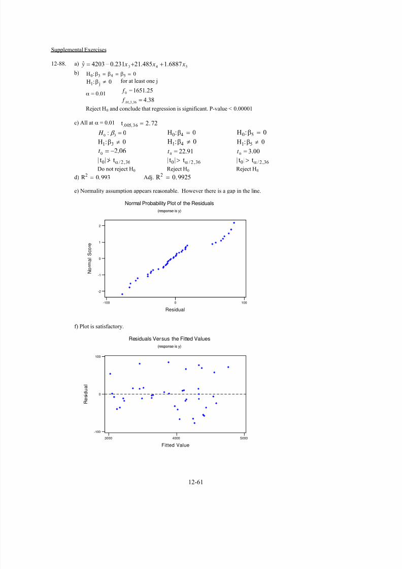
7/12/2019 Solution Manual Stats
http://slidepdf.com/reader/full/solution-manual-stats 439/588
Supplemental Exercises
12-88. a)543 6887.1485.21231.04203ˆ x x x y ++−=
b) H0 3 4 5 0:β β β= = =
H j1 0:β ≠ for at least one j
α = 0.01
38.4
25.1651
36,3,01.
0
=
=
f
f
Reject H0 and conclude that regression is significant. P-value < 0.00001
c) All at α = 0.01 t. , .005 36 2 72=
0: 30 = β H H0 4 0:β = H0 5 0:β =
H1 3 0:β ≠ H1 4 0:β ≠ H1 5 0:β ≠
06.20 −=t 91.220 =t 00.30 =t
| | / ,t t0 2/> α 36 36 36 | | / ,t t0 2> α | | / ,t t0 2> α
Do not reject H0 Reject H0 Reject H0
d) R Adj. R 2 0 993= .2 0 9925= .
e) Normality assumption appears reasonable. However there is a gap in the line.
-100 0 100
-2
-1
0
1
2
N o r m a l S c o r e
Residual
Normal Probability Plot of the Residuals
(response is y)
f) Plot is satisfactory.
3000 4000 5000
-100
0
100
Fitted Value
R e s i d
u a l
Residuals Versus the Fitted Values
(response is y)
12-61

7/12/2019 Solution Manual Stats
http://slidepdf.com/reader/full/solution-manual-stats 440/588
g) Slight indication that variance increases as x3 increases.
300002950029000
100
0
-100
x3
R e s i d u a l
Residuals Versus x3
(response is y)
h) 89.3862)1589(6887.1)170(485.21)28900(231.04203ˆ =++−= y
12-89. a) H 0 3 4 5 0:β β β∗
= = =
H j1 0:β ≠ for at least one j
α = 0.01
36,3,0
36,3,01.
0
38.4
39.1321
α f f
f
f
>>
=
=
Reject H0 and conclude that regression is significant. P-value < 0.00001
b) α = 0.01 t. , .005 36 2 72=
H0 3 0:β ∗ = H0 4 0:β = H0 5 0:β =
H1 3 0:β
∗
≠ H1 4 0:β ≠ H1 5 0:β ≠ 45.1
0 −=t 95.190 =t 53.20 =t
| | / ,t t0 2/> α 36 36 36 | | / ,t t0 2> α | | / ,t t0 2/> α
Do not reject H0 Reject H0 Do not reject H0
c) Curvature is evident in the residuals plots from this model.
Residual
P e r c e n t
0.030.020.010.00-0.01-0.02-0.03
99
95
90
80
70
60
5040
30
20
10
5
1
Normal Probabilit y Plot of t he Residuals(response is y*)
12-62

7/12/2019 Solution Manual Stats
http://slidepdf.com/reader/full/solution-manual-stats 441/588
Fitt ed Value
R e
s i d u a l
8.58.48.38.28.18.0
0.03
0.02
0.01
0.00
-0.01
-0.02
Residuals Versus the Fitted Values(response is y*)
x3*
R e s i d u a l
10.3210.3110.3010.2910.2810.2710.26
0.03
0.02
0.01
0.00
-0.01
-0.02
Residuals Versus x3*(response is y*)
12-90. From data in table 12-6
a)54321 005.0594.0454.02206.0291.086.2ˆ x x x x x y +−++−=
0: 543210 ===== β β β β β H
0oneleastat:1 ≠ j H β
α = 0.01
19,5,0
19,5,01.
0
17.4
81.4
α f f
f
f
>
=
=
Reject H0. P-value = 0.005
b) α = 0.05 093.219,025. =t
0: 10 = β H H0 2 0:β = H0 3 0:β = H0 4 0:β = H0 5 0:β =
H1 1 0:β ≠ H1 2 0:β ≠ H1 3 0:β ≠ H1 4 0:β ≠ H1 5 0:β ≠
47.20
−=t 74.20
=t 42.20 =t 80.20 −=t 26.00 =t
| | / ,t t0 2 1> α | | / ,t t0 2 19> α 19 19 199 | | / ,t t0 2> α | | / ,t t0 2> α | | / ,t t0 2/> α
Reject H0 Reject H0 Reject H0 Reject H0 Do not reject H0
c)4321 609.0455.019919.0290.0148.3ˆ x x x x y −++−=
0: 43210 ==== β β β β H
0:1 ≠ j H β for at least one j
α = 0.05
20,4,0
20,4,05.
0
87.2
28.6
α f f
f
f
>
=
=
Reject H0.
α = 0.05 t. , .025 20 2 086=
H0 1 0:β = H0 2 0:β = H0 3 0:β = H0 4 0:β =
H1 1 0:β ≠ H1 2 0:β ≠ H1 3 0:β ≠ H1 4 0:β ≠ 53.20 −=t 89.20 =t 49.20 =t 05.30 −=t
| | / ,t t0 2 2> α | | / ,t t0 2 20> α 20 200 | | / ,t t0 2> α | | / ,t t0 2> α
Reject H0 Reject H0 Reject H0 Reject H 0
d) The addition of the 5th
regressor results in a loss of one degree of freedom in the denominator and the reduction in
SS E is not enough to compensate for this loss.
12-63

7/12/2019 Solution Manual Stats
http://slidepdf.com/reader/full/solution-manual-stats 442/588
e) Observation 2 is unusually large. Studentized residuals
-0.80199 -4.99898 -0.39958 2.22883 -0.52268 0.62842 -0.45288 2.21003 1.37196
-0.42875 0.75434 -0.32059 -0.36966 1.91673 0.08151 -0.69908 -0.79465 0.27842
0.59987 0.59609 -0.12247 0.71898 -0.73234 -0.82617 -0.45518
f) R2 for model in part (a): 0.558. R2 for model in part (c): 0.557. R2 for model x1, x2, x3, x4 without obs. #2: 0.804. R2
increased because observation 2 was not fit well by either of the previous models.
g) 0: 43210 ==== β β β β H
0:1 ≠ j H β α = 0.05
19,4,05.00
19,4,05.
0
90.2
53.19
f f
f
f
>
=
=
Reject H0.
α = 0.05 t. , .025 19 2 093=
H0 1 0:β = H0 2 0:β = H0 3 0:β = H0 4 0:β =
H1 1 0:β ≠ H1 2 0:β ≠ H1 3 0:β ≠ H1 4 0:β ≠
96.30 −=t 43.60 =t 64.30 =t 39.30 −=t
19,025.00 || t t > 19,025.00 || t t > 19,025.00 || t t > 19,025.00 || t t >
Reject H0 Reject H0 Reject H0 Reject H0
h) There is some indication of curvature.
x1
R e s i d u a l
1614121086420
4
3
2
1
0
-1
-2
Residuals Versus x1(response is y)
x2
R e s i d u a l
2520151050
4
3
2
1
0
-1
-2
Residuals Versus x2(response is y)
x3
R e s i d u a l
12108642
4
3
2
1
0
-1
-2
Residuals Versus x3(response is y)
x4
R e s i d u a l
12108642
4
3
2
1
0
-1
-2
Residuals Versus x4(response is y)
12-64

7/12/2019 Solution Manual Stats
http://slidepdf.com/reader/full/solution-manual-stats 443/588
12-91. a) *
4
*
3
*
2
*
1 44.156.353.612.687.4ˆ x x x x y −−−+=
b) 0: 43210 ==== β β β β H
0oneleastat:1 ≠ j H β
α = 0.05
20,4,05.00
20,4,05.
0
87.2
79.21
f f f
f
>=
=
Reject H0 and conclude that regression is significant at α = 0.05.
α = 0.05 086.220,025. =t
H0 1 0:β = H0 2 0:β = H0 3 0:β = H0 4 0:β =
H1 1 0:β ≠ H1 2 0:β ≠ H1 3 0:β ≠ H1 4 0:β ≠
76.50 =t 96.50 −=t 90.20 −=t 99.40 −=t
20,025.00 || t t > 20,025.00 || t t > 20,025.00 || t t > 20,025.00 || t t >
Reject H0 Reject H0 Reject H0 Reject H0
c) The residual plots are more satisfactory than those in Exercise 12-90.
Fitt ed Value
R e s i d u a l
3210-1-2
1.0
0.5
0.0
-0.5
-1.0
-1.5
-2.0
Residuals Versus the Fitt ed Values(response is y*)
x1*
R e s i d u a l
0.70.60.50.40.30.2
1.0
0.5
0.0
-0.5
-1.0
-1.5
-2.0
Residuals Versus x1*(response is y*)
x2*
R e s i d u a l
0.70.60.50.40.30.2
1.0
0.5
0.0
-0.5
-1.0
-1.5
-2.0
Residuals Versus x2*(response is y*)
12-65

7/12/2019 Solution Manual Stats
http://slidepdf.com/reader/full/solution-manual-stats 444/588
x3*
R e
s i d u a l
0.70.60.50.40.3
1.0
0.5
0.0
-0.5
-1.0
-1.5
-2.0
Residuals Versus x3*(response is y*)
x4*
R e
s i d u a l
3.53.02.52.01.5
1.0
0.5
0.0
-0.5
-1.0
-1.5
-2.0
Residuals Versus x4*(response is y*)
12-92. a) 20006.0023.2405.1709ˆ x x y −+−=
b) 0: 1110 == β β H
0oneleastat:1 ≠ j H β
α = 0.05
7,2,05.00
7,2,05.
0
74.411.300
f f
f f
>>
==
Reject H0.
c) H 0 11 0:β =
H1 11 0:β ≠
α = 0.05
7,1,0
7,1,05.
0
111
0
59.5
01.55
04413.0
1/4276.2/)|(
α
β β
f f
f
f
MS
r SSF
E
R
>>
=
=
==
Reject H0.
d) There is some indication of non-constant variance.
161514131211
0.3
0.2
0.1
0.0
-0.1
-0.2
-0.3
Fitted Value
R e s i d u a l
Residuals Versus the Fitted Values
(response is y)
12-66

7/12/2019 Solution Manual Stats
http://slidepdf.com/reader/full/solution-manual-stats 445/588
e.) Normality assumption is reasonable.
-0.3 -0.2 -0.1 0.0 0.1 0.2 0.3
-1
0
1
N o r m a l S c o r e
Residual
Normal Probability Plot of the Residuals(response is y)
12-93. a)54
*
3
* 000418.00055.0404.1068.21ˆ x x x y ++−=
013156.0= E MS 0.4= pC
b) Same as model in part (a)
c) x4, x5 with and1.4= pC 0134.0= E MS
d) The model in part (c) is simpler with values for MS E and C p similar to those in part (a) and (b). The part (c) model is
preferable.
e) 4.52)ˆ( 3 =∗ β VIF
3.9)ˆ( 4 = β VIF
1.29)ˆ( 5 = β VIF
Yes, VIFs for x and x exceed 103*
5
12-94. a) *
4
*
3
*
2
*
1 44.156.353.612.687.4ˆ x x x x y −−−+=
41642.0)( = p MS E Min 0.5= pC
b) Same as part (a)
c) Same as part (a)
d) All models are the same.
12-95. a)21 4.1085.00.300ˆ x x y ++=
8.405)2(4.10)100(85.0300ˆ =++= y
b) S yy = 1230 5. SSE = 120 3.
2.11103.1205.1230 =−=−= E yy R SSSSS
37.55025.10
1.555
025.10315
3.120
1.5552
2.1110
0 ===
=−
=−
=
===
E
R
E
E
R
R
MS
MS f
pn
SS MS
k
SS MS
H0 1 2 0:β β= =
0oneleastat:1 ≠ j H β
α = 0.05
12-67

7/12/2019 Solution Manual Stats
http://slidepdf.com/reader/full/solution-manual-stats 446/588
12,2,05.00
12,2,05.
0
89.3
37.55
f f
f
f
>
=
=
Reject H0 and conclude that the regression model is significant at α = 0.05
c) 9022.05.12302.11102 ===
yy
R
SSS R or 90.22%
d) k = 3 p = 4 SSE ' .= 117 20
65.1011
2.117'' ==
−=
pn
SS MS E
E
No, MSE increased with the addition of x3 because the reduction in SSE was not enough to compensate for the loss in
one degree of freedom in the error sum of squares. This is why MS E can be used as a model selection criterion.
e) 30.111320.1175.1230 =−=−= E yy R SSSSS
1.3
20.111030.1113
)|,()|(),,|( 01201230123
=
−=
−= β β β β β β β β β β β R R R SSSSSS
0: 30 = β H
0: 31 ≠ β H
α = 0.05
11,1,05.00
11,1,05.
01230
84.4
291.011/2.117
1/1.3
/'
/),,|(
f f
f
pnSS
r SS f
E
R
>/
=
==−
=β β β β
Do not reject H0.
12-96. a)
The model with the minimum C p (-1.3) value is:W = 69.9 + 0.120 HR_B + 0.0737 BB_B - 0.0532 SO_B + 0.0942 SB
The model assumptions are not violated as shown in the graphs below.
Where X1 = AVG, X2 = R, X3 = H, X4 = 2B, X5 = 3B, X6 = HR, X7 = RBI, X8 = BB, X9 = SO, X10 = SB
X11 = GIDP, X12 = LOB and X13 = OBP
The model assumptions appear reasonable.
Standardized Residual
S c o r e
3210-1-2-3
2
1
0
-1
-2
Normal Probabi l i ty Plot o f the Residuals(response is W)
12-68

7/12/2019 Solution Manual Stats
http://slidepdf.com/reader/full/solution-manual-stats 447/588
Fitted Value
S t a n d a r d
i z e d
R e s i d u a l
10095908580757065
2
1
0
-1
-2
Residuals Versus the Fi t t ed Values(response is W)
SB
S t a n d a r d
i z e d
R e s i d u a l
16014012010080604020
2
1
0
-1
-2
Residuals Ver sus SB(response is W)
SO_B
S t a n d a r d i z e d
R e s i d u a l
1300120011001000900800
2
1
0
-1
-2
Residuals Ver sus SO_B(response is W)
BB_B
S
t a n d a r d i z e d
R e s i d u a l
650600550500450400
2
1
0
-1
-2
Residuals Ver sus BB_B(response is W)
HR_B
S t a n d a r d i z e d
R e s i d u a l
260240220200180160140120100
2
1
0
-1
-2
Residuals Ver sus HR_B(response is W)
b)
Minimum C p (1.1) model:W = 96.5 + 0.527 SV - 0.125 HR_P - 0.0847 BB_P + 0.0257 SO_P
12-69

7/12/2019 Solution Manual Stats
http://slidepdf.com/reader/full/solution-manual-stats 448/588
Based on the graphs below, the model assumptions are not violated
Standardized Residual
S c o r e
3210-1-2-3
2
1
0
-1
-2
Normal Probabi l i ty Plot o f the Residuals(response is W)
Fitted Value
S t a n d a r d i z e d
R e s i d u a l
10090807060
2
1
0
-1
-2
Residuals Versus the Fi t t ed Values(response is W)
SV
S t a n d a r d i z
e d
R e s i d u a l
55504540353025
2
1
0
-1
-2
Residuals Ver sus SV(response is W)
HR_P
S t a n d a
r d i z e d
R e s i d u a l
220200180160140120
2
1
0
-1
-2
Residuals Ver sus HR_P(response is W)
12-70
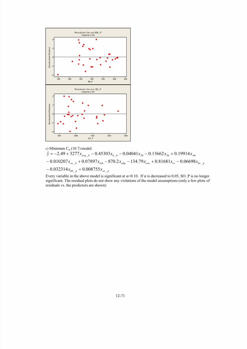
7/12/2019 Solution Manual Stats
http://slidepdf.com/reader/full/solution-manual-stats 449/588
BB_P
S t a n d a r d
i z e d
R e s i d u a l
650600550500450400350
2
1
0
-1
-2
Residuals Ver sus BB_P(response is W)
SO_P
S t a n d a r d i z e d
R e s i d u a l
1300120011001000900
2
1
0
-1
-2
Residuals Ver sus SO_P(response is W)
c) Minimum C p (10.7) model:
pso pbb
phr er eraobplobbso
rbibbbhbavg
x x
x x x x x x
x x x x x y
_ _
_ _
32 _ _
008755.0032314.0
06698.081681.079.1342.87007897.0010207.0
19914.013662.004041.045303.0327749.2ˆ
+−
−+−−+−
+−−−+−=
Every variable in the above model is significant at α=0.10. If α is decreased to 0.05, SO_P is no longer
significant. The residual plots do not show any violations of the model assumptions (only a few plots of residuals vs. the predictors are shown)
12-71

7/12/2019 Solution Manual Stats
http://slidepdf.com/reader/full/solution-manual-stats 450/588
Standardized Residual
S c o r e
3210-1-2-3
2
1
0
-1
-2
Normal P robab i l i t y P l o t o f t he Resi dua l s(response is W)
Fitted Value
S t a
n d a r d i z e d
R e s i d u a l
1009080706050
2
1
0
-1
-2
Residuals Versus the Fi t t ed Values(response is W)
SO_B
S t a n d a r d i z e d
R e s i d u a l
1300120011001000900800
2
1
0
-1
-2
Residuals Versus SO_B(response is W)
AVG_B
S t a n d a r d i z e d
R e s i d u a l
0.2850.2800.2750.2700.2650.2600.2550.250
2
1
0
-1
-2
Residuals Versus AVG_B(response is W)
ERA
S t a n d a r d i z e d
R e s i d u a l
5.55.04.54.03.5
2
1
0
-1
-2
Residuals Ver sus ERA(response is W)
12-97. a)
yy
R
S
SS R =2
12-72

7/12/2019 Solution Manual Stats
http://slidepdf.com/reader/full/solution-manual-stats 451/588
03.047.05.0
47.0)50.0(94.0)(2
=−=−=
===
R yy E
yy R
SSSSS
S RSS
0...: 6210 ==== β β β H
0oneleastat:1 ≠ j H β
α = 0.05
7,6,05.00
7,6,05.
0
87.3
28.187/03.0
6/47.0
/
/
f f
f
pnSS
k SS f
E
R
>
=
==−
=
Reject H0.
b) k = 5 n = 14 p = 6 R2 0 92= .
04.046.05.0''
46.0)50.0(92.0)(' 2
=−=−=
===
R yy E
yy R
SSSSS
S RSS
01.0
46.047.0
)()()|,( 06,,2,1,0
=
−=
−== reduced SS fullSSSS R Rii j R β β ββ …
8,1,05.00
8,1,05.
06,,2,1,
0
32.5
28/04.0
1/01.0
)/('
/)|,(
f f
f
pnSS
r SS f
E
ii j R
>/
=
==−
== β β β
…
Do not reject H0. There is not sufficient evidence that the removed variable is significant at α = 0.05.
c) 005.08
04.0)( ==
−=
pn
SSreduced MS E
E
004.07
03.0)( == full MS E
No, the MS E is larger for the reduced model, although not by much. Generally, if adding a variable to a model
reduces the MS E it is an indication that the variable may be useful in explaining the response variable. Here the
decrease in MS E is not very great because the added variable had no real explanatory power.
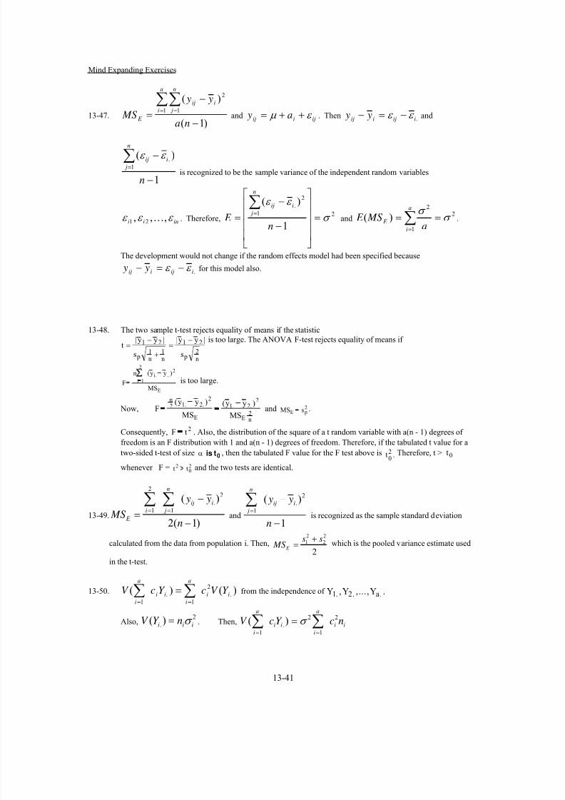
7/12/2019 Solution Manual Stats
http://slidepdf.com/reader/full/solution-manual-stats 452/588
Mind Expanding Exercises
13-47.)1(
)(1 1
2
−
−
=∑∑
= =
na
y y
MS
a
i
n
j
iij
E and ijiij a y ε μ ++= . Then .iijiij y y ε ε −=− and
1
)(1
.
−
−∑=
n
n
j
iij ε ε
is recognized to be the sample variance of the independent random variables
inii ε ε ε ,,, 21 … . Therefore,21
2
.
1
)(
σ
ε ε
=
⎥⎥⎥⎥
⎦
⎤
⎢⎢⎢⎢
⎣
⎡
−
−
=∑
=
n E
n
j
iij
and2
1
2
)( σ σ
== ∑=
a
i
E a
MS E .
The development would not change if the random effects model had been specified because
.iijiij y y ε ε −=− for this model also.
13-48. The two sample t-test rejects equality of means if the statistic
ty y
s
y y
s p n n p n
=−
+=
−| | | | is too large. The ANOVA F-test rejects equality of means if 1 2
1 1
1 2
2
E
2...i
2
1i
MS
)yy(n
F
−
=
∑= is too large.
Now,
n2E
2.2.1
E
2.2.12
n
MS
)yy(
MS
)yy(F
−=
−= and .2
pEsMS =
Consequently, . Also, the distribution of the square of a t random variable with a(n - 1) degrees of
freedom is an F distribution with 1 and a(n - 1) degrees of freedom. Therefore, if the tabulated t value for a
two-sided t-test of size , then the tabulated F value for the F test above is t Therefore, t >
whenever F = and the two tests are identical.
2tF =
0tis α02 . 0t
20
2 tt >
13-49.)1(2
)( 2
.
1
2
1
−
−
=∑∑
==
n
y y
MS
iij
n
ji
E and1
)( 2
.
1
−
−∑=
n
y y iij
n
jis recognized as the sample standard deviation
calculated from the data from population i. Then,
2
2
2
2
1 ss MS E
+= which is the pooled variance estimate used
in the t-test.
13-50. from the independence of Y Y )()( .
2
1
.
1
ii
a
i
ii
a
i
Y V cY cV ∑∑==
= Ya1 2. ., ,..., ..
Also, . Then,2
.)(iii nY V σ =
ii
a
i
ii
a
i
ncY cV 2
1
2
.
1
)( ∑∑==
= σ
13-41

7/12/2019 Solution Manual Stats
http://slidepdf.com/reader/full/solution-manual-stats 453/588
13-51. If b, c, and d are the coefficients of three orthogonal contrasts, it can be shown that
a
y
y
d
yd
c
yc
b
yb i
a
ii
a
ii
a
i
ii
a
i
i
a
i
ii
a
i
i
a
i
ii
i
2
.
12
.
12
1
2
.
1
2
1
2
.
1
2
1
2
.
4
1
)()()()( ∑∑
∑
∑
∑
∑
∑
∑=
=
=
=
=
=
=
= −=++ always holds. Upon dividing both sides
by n, we have N
y
n
yQQQ i
a
i
2..
2
1
2
3
2
2
2
1 −=++ ∑=
which equals . The equation above can be
obtained from a geometrical argument. The square of the distance of any point in four-dimensional space from the zero
point can be expressed as the sum of the squared distance along four orthogonal axes. Let one of the axes be the 45
degree line and let the point be ( ). The three orthogonal contrasts are the other three axes. The square of
the distance of the point from the origin is and this equals the sum of the squared distances along each of the
four axes.
SStreatments
.4.3.2.1 ,,, y y y y
2
.
1
i
a
i
y∑=
13-52. Because2
2
12 )(
σ
μ μ
a
n i
a
i −=Φ ∑=, we only need to shows that
2
1
2
)(2
μ μ −≤ ∑=
i
a
i
D.
Let μ1 and μ2 denote the means that differ by D. Now, is minimized for x equal
to the mean of μ
2
2
2
1 )()( x x −+− μ μ
1 and μ2. Therefore,
2
1
2
2
2
1
2212
2211 )()()()
2
+-()
2
+-( μ μ μ μ μ μ
μ μ μ
μ μ μ −≤−+−≤+ ∑
=i
a
i
Then, 2
1
2222
12
2
21 )(24422
μ μ μ μ μ μ
−≤=+=⎟ ⎠
⎞⎜⎝
⎛ −+⎟
⎠
⎞⎜⎝
⎛ −∑
=i
a
i
D D D.
13-53.a
s
na
y y
MSi
a
i
iij
n
j
a
i
E
2
1
2
.
11
)1(
)(
∑∑∑ === =−
−
= where1
)( 2
.
12
−
−
= ∑=
n
y y
s
iij
n
j
i . Because s is the
sample variance of
i2
,,...,, 21 inii y y y2
2)1(
σ
iSn −has a chi-square distribution with n-1 degrees of
freedom. Then, a n MSE( )− 1
2σis a sum of independent chi-square random variables. Consequently,
a n MSE( )− 1
2σhas a chi-square distribution with a(n - 1) degrees of freedom. Consequently,
⎟⎟
⎠
⎞⎜⎜
⎝
⎛ −≤≤
−=
−=≤−
≤
−−−
−−−
2
)1(,2
1
2
)1(,2
2
)1(,2
2
)1(,2
1
)1()1(
1))1(
(
2
2
nana
nana
E E
E
MSna MSnaP
MSnaP
α α
α α
χ σ
χ
α χ σ
χ
Using the fact that a(n - 1) = N - a completes the derivation.
13-42

7/12/2019 Solution Manual Stats
http://slidepdf.com/reader/full/solution-manual-stats 454/588
13-54. From Exercise 13-53,2
)(
σ
E MSa N −has a chi-square distribution with N - a degrees of freedom. Now,
nY V i
22
. )(σ
σ τ
+= and mean square treatment = is n times the sample variance of T MS
.,...,, ..2.1 a y y y Therefore, 222
)1(
)(
)1(2
σ σ σ τ
σ
τ +
−=+
−
n
MSa
n
MSa T
n
T
has a chi-squared distribution with a - 1
degrees of freedom. Using the independence of MST and MSE, we conclude that
⎟ ⎠
⎞⎜⎝
⎛ ⎟⎟ ⎠
⎞⎜⎜⎝
⎛
+ 222/
σ σ σ τ
E T MS
n
MShas an F distribution.a N( ) ,(− −1 a)
Therefore,
⎟⎟ ⎠
⎞
⎜⎜⎝
⎛
⎥⎦
⎤
⎢⎣
⎡
−≤≤⎥⎦
⎤
⎢⎣
⎡
−=
−=≤+
≤
−−−−−
−−−−−
1
1
1
1
1)(
,1,2
1,1,2
22
1
2
2
1
,1,22
2
,1,1
E
T
f E
T
f
a N a
E
T
a N a
MS
MS
n MS
MS
nP
f n MS
MS f P
a N aa N aα α
α α
σ
σ
α σ σ
σ
τ
τ
by an algebraic solution for σ
στ2
2
and )(2
2
U LP ≤≤σ
σ τ .
13-55. a) As in Exercise 13-54,22
2
σ σ
σ
τ +n MS
MS
E
T has an F distribution.a N( ) ,(− −1 a)
and
)11
(
)11
111
(
)11
(
)(1
22
2
2
2
2
2
2
2
+≤
+≤
+=
+≤+≤+=
≤≤=
≤≤=−
U
U
L
LP
LU P
LU P
U LP
τ
τ
τ
τ
τ
σ σ
σ
σ
σ
σ
σ
σ
σ α
13-43

7/12/2019 Solution Manual Stats
http://slidepdf.com/reader/full/solution-manual-stats 455/588
b)
)1
1
1
1(
)11(
)11
1(
)(1
22
2
2
22
2
2
2
2
+≤
+≤
+=
+≤+
≤+=
+≤+
≤+=
≤≤=−
LU P
U LP
U LP
U LP
τ
τ
τ
τ
σ σ
σ
σ
σ σ
σ
σ
σ
σ α
Therefore, )1
1,
1
1(
++ LU is a confidence interval for
σ
σ στ
2
2 2+
13-56. 1
)( 2
...
1
−
−
=
∑=
a
y yn
MS
ii
a
i
T and for any random variable X , E X .V X E X( ) ( ) [ ( )]2 2
= +Then,
1
})]([)({
)(
2
......
1
−
−+−=
∑=
a
Y Y E Y Y V n
MS E iii
a
iT
Now,aan N a N n N N n N n N n
Y Y Y Y Y Y Y Y 11
12
121
11
1111
11...1 .........)(...)(
2111−−−−−−−−++−=−
and
constraint thefrom...)()(
)()()(
122
1111
...1
2112
2
11
211...1
1
11
τ τ τ τ
σ σ
=−−−−=−
−=⎟ ⎠
⎞⎜⎝
⎛ −+−=−
aa
N n
N n N n
N n
N nnY Y E
N
n N nY Y V
Then,
2 2 2 21 1
1 1
2
2 1
{( ) } [(1 ) ]
( )1 1
1
i
i
a an
n N N i i
i iT
a
i i
i
n n
E MSa a
n
a
i iσ τ σ
τ
σ
= =
=
− + − += =
− −
= +−
∑ ∑
∑
τ
Because , this does suggest that the null hypothesis is as given in the exercise.2)( σ = E MS E
13-57. a) If A is the accuracy of the interval, then At
n
MS
na
E =−
2
)1(,2
α
Squaring both sides yields222
)1(,2
At n
MS
na
E =−α
As in Exercise 13-48, )1(,1,
2
)1(,2
−−= nana
F t α α . Then,
2
)1(,1,2
A
F MSn
na E −= α
13-44

7/12/2019 Solution Manual Stats
http://slidepdf.com/reader/full/solution-manual-stats 456/588
b) Because n determines one of the degrees of freedom of the tabulated F value on the right-side of the equation in part (a),
some approximation is needed. Because the value for a 95% confidence interval based on a normal distribution is 1.96, w
approximate)1(,
2−na
t α by 2 and we approximate
)1(,1,
2
)1(,2
−−= nana
F t α α by 4.
Then, 84
)4)(4(2 ==n . With n = 8, a(n - 1) = 35 and F .0 05135 4 12. , , .=
The value 4.12 can be used for F in the equation for n and a new value can be computed for n as
824.84
)12.4)(4(2≅==n
Because the solution for n did not change, we can use n = 8. If needed, another iteration could be used to
refine the value of n.
13-45

7/12/2019 Solution Manual Stats
http://slidepdf.com/reader/full/solution-manual-stats 457/588
CHAPTER 13
Section 13-2
13-1. a) Analysis of Variance for STRENGTHSource DF SS MS F P
COTTON 4 475.76 118.94 14.76 0.000Error 20 161.20 8.06Total 24 636.96
Reject H0 and conclude that cotton percentage affects mean breaking strength.
3530252015
25
15
5
COTTON
S T R E N G T H
b) Tensile strength seems to increase up to 30% cotton and declines at 35% cotton.
Cotton Percentage
M e a n S t r e n g t h
3530252015
22
20
18
16
14
12
10
Scatt erplot of Mean Strength vs Cotton Percentage
Individual 95% CIs For MeanBased on Pooled StDev
Level N Mean StDev ------+---------+---------+---------+15 5 9.800 3.347 (-----*----)20 5 15.400 3.130 (----*----)
25 5 17.600 2.074 (----*----)30 5 21.600 2.608 (----*----)35 5 10.800 2.864 (-----*----)
------+---------+---------+---------+Pooled StDev = 2.839 10.0 15.0 20.0 25.0
c) The normal probability plot and the residual plots show that the model assumptions are reasonable.
13-1

7/12/2019 Solution Manual Stats
http://slidepdf.com/reader/full/solution-manual-stats 458/588
201510
6
5
4
3
2
1
0
-1
-2
-3
-4
FittedValue
R e s i d u a l
ResidualsVersus the Fitted Values(response is STRENGTH)
210-1-2
6
5
4
3
2
1
0
-1
-2
-3
-4
Normal Score
R e s i d u a l
Normal Probability Plot of the Residuals(response is STRENGTH)
352515
6
5
4
3
2
1
0
-1
-2
-3
-4
COTTON
R e s i d u a l
Residuals Versus COTTON(response is STRENGTH)
13-2 a) Analysis of Variance for FLOW
Source DF SS MS F PFLOW 2 3.6478 1.8239 3.59 0.053Error 15 7.6300 0.5087Total 17 11.2778
Do not reject H0. There is no evidence that flow rate affects etch uniformity.
200160125
5
4
3
FLOW
U N I F O R M I T
b) Residuals are acceptable.
-1 0 1
-2
-1
0
1
2
N o r m a l S c o r e
Residual
Normal Probability Plot of the Residuals(response is obs)
13-2

7/12/2019 Solution Manual Stats
http://slidepdf.com/reader/full/solution-manual-stats 459/588
200190180170160150140130120
1
0
-1
FLOW
R
e s i d u a l
Residual s VersusFLOW(response is UNIFORMI)
4.54.03.5
1
0
-1
FittedValue
R e s i d u a l
Residuals Versus the Fitted Values(response is UNIFORMI)
13-3. a) Analysis of Variance for STRENGTHSource DF SS MS F PTECHNIQU 3 489740 163247 12.73 0.000Error 12 153908 12826Total 15 643648
Reject H0. Techniques affect the mean strength of the concrete.
b) P-value ≅ 0
c) Residuals are acceptable
4321
200
100
0
-100
-200
TECHNIQU
R e s i d u a l
Residuals VersusTECHNIQU(response is STRENGTH)
315030502950285027502650
200
100
0
-100
-200
FittedValue
R e s i d u a l
Residuals Versus the Fitted Values(response i s STRENGTH)
-200 -100 0 100 200
-2
-1
0
1
2
N o r m a l S c o r e
Residual
Normal Probability Plot of the Residuals(response is STRENGTH)
13-3

7/12/2019 Solution Manual Stats
http://slidepdf.com/reader/full/solution-manual-stats 460/588
13-4 a) Analysis of Variance for CIRCUIT TYPESource DF SS MS F PCIRCUITT 2 260.9 130.5 4.01 0.046Error 12 390.8 32.6Total 14 651.7
Reject H0
b)There is some indication of greater variability in circuit two. There is some curvature in the normal probability plot.
-10 0 10
-2
-1
0
1
2
N o r m a l S c o r e
Residual
Normal Probability Plot of the Residuals(response is time)
321
10
0
-10
CIRCUITT
R e s i d u a l
ResidualsVersusCIRCUITT(response is RESPONSE)
282318
10
0
-10
FittedValue
R e s i d u a l
Residuals Versus the Fitted Values(response is RESPONSE)
c) 95% Confidence interval on the mean of circuit type 3.
96.2384.12
5
6.32179.24.18
5
6.32179.24.18
1
1
12,025.0312,025.03
≤≤
+≤≤−
+≤≤−
μ
μ
μ n
MSt y
n
MSt y E
i
E
13-5. a) Analysis of Variance for CONDUCTIVITYSource DF SS MS F P
COATINGTYPE 4 1060.5 265.1 16.35 0.000Error 15 243.3 16.2Total 19 1303.8
Reject H0, P-value ≅ 0
13-4

7/12/2019 Solution Manual Stats
http://slidepdf.com/reader/full/solution-manual-stats 461/588
b) There is some indication of that the variability of the response may be increasing as the mean response
increases. There appears to be an outlier on the normal probability plot.
54321
5
0
-5
-10
COATINGT
R e s i d u a l
Residuals Versus COATINGT(response is CONDUCTI)
145140135130
5
0
-5
-10
FittedValue
R e s i d u a l
ResidualsVersusthe Fitted Values(response is CONDUCTI)
-10 -5 0 5
-2
-1
0
1
2
N o r m a l S c o r e
Residual
Normal Probability Plot of the Residuals(response is CONDUCTI)
c) 95% Confidence interval on the mean of coating type 1
29.14971.140
4
2.16131.200.145
4
2.16131.200.145
1
1
15,015.0115,025.01
≤≤
+≤≤−
+≤≤−
μ
μ
μ n
MS
t yn
MS
t y
E
i
E
99% confidence interval on the difference between the means of coating types 1 and 4.
14.2436.7
4
)2.16(2947.2)25.12900.145(4
)2.16(2947.2)25.12900.145(
22
41
41
15,005.0414115,005.041
≤−≤
−−≤−≤−−
+−≤−≤−−
μ μ
μ μ
μ μ n
MSt y y
n
MSt y y E E
13-5

7/12/2019 Solution Manual Stats
http://slidepdf.com/reader/full/solution-manual-stats 462/588
13-6 a) Analysis of Variance for ORIFICE Source DF SS MS F PORIFICE 5 1133.37 226.67 30.85 0.000Error 18 132.25 7.35Total 23 1265.63
Reject H0
b) P-value ≅ 0
c)
2.01.51.00.5
4
3
2
1
0
-1
-2
-3
-4
-5
ORIFICE
R e s i d u a l
Residuals VersusORIFICE(response is RADON)
807060
4
3
2
1
0
-1
-2
-3
-4
-5
FittedValue
R e s i d u a l
Residuals Versusthe Fitted Values(response is RADON)
-5 -4 -3 -2 -1 0 1 2 3 4
-2
-1
0
1
2
N o r m a l S c o r e
Residual
Normal Probability Plot of the Residuals(response is percent)
d) 95% CI on the mean radon released when diameter is 1.40
84.6715.62
4
35.7101.265
4
35.7101.265
1
1
18,015.0518,025.05
≤≤
+≤≤−
+≤≤−
μ
μ
μ n
MSt y
n
MSt y E
i
E
13-6

7/12/2019 Solution Manual Stats
http://slidepdf.com/reader/full/solution-manual-stats 463/588
13-7. a) Analysis of Variance for STRENGTHSource DF SS MS F PRODDING 3 28633 9544 1.87 0.214Error 8 40933 5117Total 11 69567
Do not reject H0
b) P-value = 0.214
c) The residual plot suggests nonconstant variance. The normal probability plot looks acceptable.
25201510
100
0
-100
RODDING
R e s i d u a l
Residuals Versus RODDING(response is STRENGTH)
160015501500
100
0
-100
FittedValue
R e s i d u a l
ResidualsVersusthe Fitted Values(response is STRENGTH)
-100 0 100
-2
-1
0
1
2
N o r m a l S c o r e
Residual
Normal Probability Plot of the Residuals(response is STRENGTH)
13-8 a) Analysis of Variance of PREPARATION METHODSource DF SS MS F PPREPMETH 3 22.124 7.375 14.85 0.000Error 16 7.948 0.497Total 19 30.072
Reject H0
b) P-value ≅ 0
c) There are some differences in the amount variability at the different preparation methods and there is some
curvature in the normal probability plot. There are also some potential problems with the constant variance
assumption apparent in the fitted value plot.
13-7

7/12/2019 Solution Manual Stats
http://slidepdf.com/reader/full/solution-manual-stats 464/588
4321
1
0
-1
-2
PREPMETH
R e s i d u a l
Residuals Versus PREPMETH(response is TEMPERAT)
15141312
1
0
-1
-2
FittedValue
R e s i d u a l
Residuals Versus the Fitted Values(response is TEMPERAT)
-2 -1 0 1
-2
-1
0
1
2
N o r m a l S c o r e
Residual
Normal Probability Plot of the Residuals(response is temp)
d) 95% Confidence interval on the mean of temperature for preparation method 1
47.1513.14
5
497.0120.28.14
5
497.0120.28.14
1
3
16,015.0116,025.01
≤≤
+≤≤−
+≤≤−
μ
μ
μ n
MSt y
n
MSt y E
i
E
13-9. a) Analysis of Variance for STRENGTHSource DF SS MS F PAIRVOIDS 2 1230.3 615.1 8.30 0.002Error 21 1555.8 74.1Total 23 2786.0
Reject H0
b) P-value = 0.002
c) The residual plots indicate that the constant variance assumption is reasonable. The normal probability
plot has some curvature in the tails but appears reasonable.
13-8
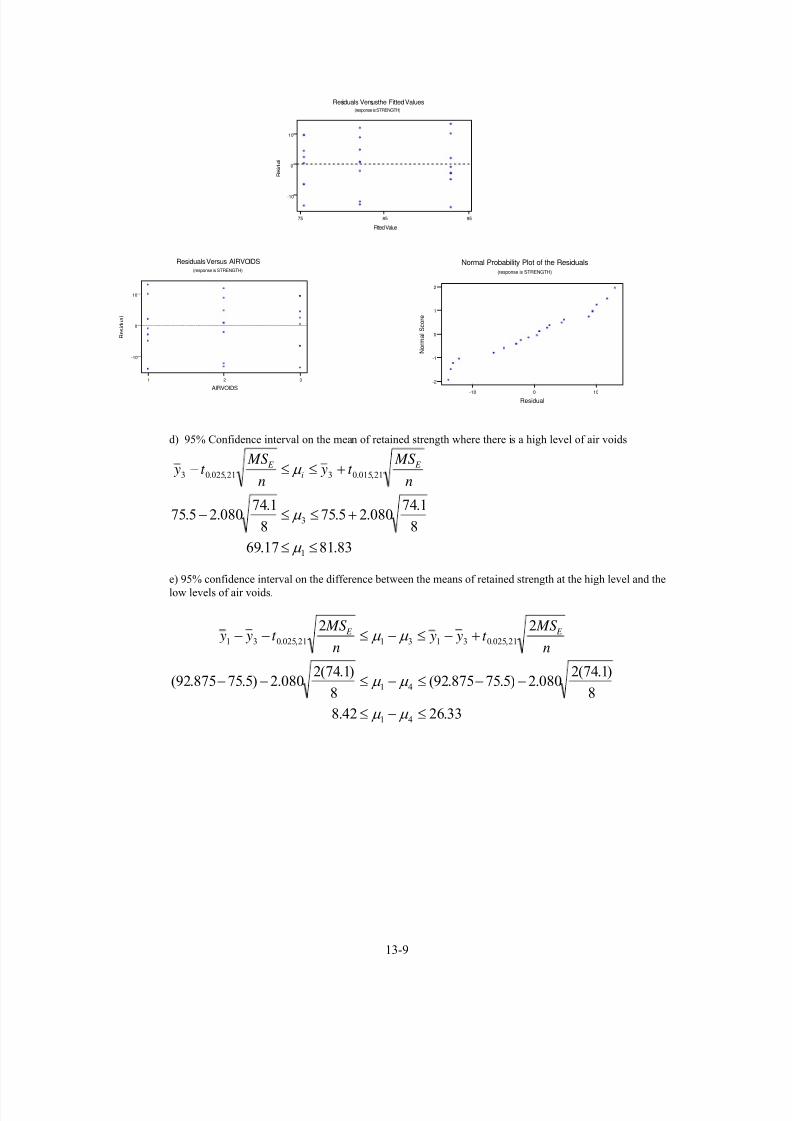
7/12/2019 Solution Manual Stats
http://slidepdf.com/reader/full/solution-manual-stats 465/588
958575
10
0
-10
FittedValue
R e s i d u a l
Residuals Versusthe Fitted Values(response is STRENGTH)
100-10
2
1
0
-1
-2
N o r m a l S c o r e
Residual
Normal Probability Plot of the Residuals(response is STRENGTH)
321
10
0
-10
AIRVOIDS
R e s i d u a l
Residuals Versus AIRVOIDS(response is STRENGTH)
d) 95% Confidence interval on the mean of retained strength where there is a high level of air voids
83.8117.69
8
1.74080.25.75
8
1.74080.25.75
1
3
21,015.0321,025.03
≤≤
+≤≤−
+≤≤−
μ
μ
μ n
MSt y
n
MSt y E
i
E
e) 95% confidence interval on the difference between the means of retained strength at the high level and thelow levels of air voids.
33.2642.8
8
)1.74(2080.2)5.75875.92(
8
)1.74(2080.2)5.75875.92(
22
41
41
21,025.0313121,025.031
≤−≤
−−≤−≤−−
+−≤−≤−−
μ μ
μ μ
μ μ n
MSt y y
n
MSt y y E E
13-9

7/12/2019 Solution Manual Stats
http://slidepdf.com/reader/full/solution-manual-stats 466/588
13-10. a)
ANOVA
Source DF SS MS F PFactor 5 2.5858 0.5172 18.88 0.000Error 30 0.8217 0.0274Total 35 3.4075
D a t a
10.50-0.5-0.75Crosslinker Level -1
9.2
9.0
8.8
8.6
8.4
8.2
8.0
Boxplot of Crosslinker Level -1, -0.75 , -0.5, 0, 0.5 , 1
Yes, the box plot and ANOVA show that there is a difference in the cross-linker level.
b) Anova table in part (a) showed the p-value = 0.000 < α = 0.05. Therefore there is at least one
level of cross-linker is different. The variability due to random error is SSE = 0.8217
c) Domain spacing seems to increase up to the 0.5 cross-linker level and declines once cross-
linker level reaches 1.
Cross-linker lev el
M e a n d o m a i n s
p a c i n g
1.00.50.0-0.5-1.0
8.9
8.8
8.7
8.6
8.5
8.4
8.3
8.2
8.1
8.0
Scatterplot of Mean domain spacing vs Cross-linker level
13-10

7/12/2019 Solution Manual Stats
http://slidepdf.com/reader/full/solution-manual-stats 467/588
d) The normal probability plot and the residual plots show that the model assumptions are
reasonable.
Residual
P e r c e n t
0.40.20.0-0.2-0.4
99
90
50
10
1
Fitted Value
R e s i d u a l
8.88.68.48.28.0
0.2
0.0
-0.2
-0.4
Residual
F r e q u e
n c y
0.30.20.10.0-0.1-0.2-0.3
6.0
4.5
3.0
1.5
0.0
Observ ation Order
R e s i d u a l
35302520151051
0.2
0.0
-0.2
-0.4
Normal Probab ilit y Plo t o f the Residuals Residuals Versus t he Fit ted Values
Hist o gram of t he Residuals Residuals Versus t h e Order of t he Dat a
Residual Plots for Domain spacing
13-11. a) No, the diet does not affect the protein content of cow’s milk.
Comparative boxplots
C4
C 3
lupinsBarley+lupinsBarley
4.5
4.0
3.5
3.0
2.5
Boxp lo t o f C3 by C4
ANOVA
Source DF SS MS F PC4 2 0.235 0.118 0.72 0.489
Error 76 12.364 0.163
Total 78 12.599
S = 0.4033 R-Sq = 1.87% R-Sq(adj) = 0.00%
b) P-value = 0.489. The variability due to random error is SSE = 0.146.
13-11

7/12/2019 Solution Manual Stats
http://slidepdf.com/reader/full/solution-manual-stats 468/588
c) The Barley diet has the highest average protein content and lupins the lowest.
Diet type
m
e a n p r o t e i n
LupinsBarley+LupinsBarley
3.900
3.875
3.850
3.825
3.800
3.775
3.750
Sca t te rp lo t o f m ean p ro te in vs d ie t type
d) Based on the residual plots, there is no violation of the ANOVA assumptions.
Residual
S c o r e
1.51.00.50.0-0.5-1.0
3
2
1
0
-1
-2
-3
Normal Probabi l i ty Plo t o f the Residuals
(response i s protein content)
Fitted Value
R e s i d u a l
3.9003.8753.8503.8253.8003.7753.750
0.5
0.0
-0.5
-1.0
Residuals Versus the Fi t t ed Values(response i s protein content)
Diet
R E S I 1
LupinsBarley+LupinsBarley
0.5
0.0
-0.5
-1.0
Scatter p lo t o f RESI 1 v s Diet
13-12

7/12/2019 Solution Manual Stats
http://slidepdf.com/reader/full/solution-manual-stats 469/588
13-12. a) From the analysis of variance shown below, 07.48,3,05.0 =F > F 0 = 3.43 there is no
difference in the spoilage percentage when using different AO solutions.
ANOVA
Source DF SS MS F PAO solutions 3 3364 1121 3.43 0.073Error 8 2617 327Total 11 5981
b) From the table above, the P-value = 0.073 and the variability due to random error is SSE =
2617.
c) A 400ppm AO solution should be used because it produces the lowest average spoilage
percentage.
AO solut ion
A v g .
S p o i l a g e
4003002001000
70
60
50
40
30
20
Scatterplot of Avg. Spoilage vs AO solution
d) The normal probability plot and the residual plots show that the model assumptions are
reasonable.
Residual
P e r c e n t
40200-20-40
99
90
50
10
1
Fitted Value
R e s i d u a
l
7060504030
20
0
-20
Residual
F r e q u e n c y
3020100-10-20
4
3
2
1
0
Observat ion Order
R e s i d u a l
121110987654321
20
0
-20
No rm al Prob ab ilit y Plo t o f t h e Resid u als Resid u als Versu s t h e Fit t ed Valu es
Hist ogram of t he Residuals Residuals Versus t he Order of t he Dat a
Residual Plots f or % Spoilage
13-13 a) Analysis of Variance for TEMPERATURESource DF SS MS F PTEMPERAT 3 0.1391 0.0464 2.62 0.083Error 18 0.3191 0.0177
13-13

7/12/2019 Solution Manual Stats
http://slidepdf.com/reader/full/solution-manual-stats 470/588
Total 21 0.4582
Do not reject H0
b) P-value = 0.083
c) Residuals are acceptable
-0.2 -0.1 0.0 0.1 0.2
-2
-1
0
1
2
N o r m a l S c o r e
Residual
Normal Probability Plot of the Residuals
(response is density)
180170160150140130120110100
0.2
0.1
0.0
-0.1
-0.2
TEMPERAT
R e s i d u a l
Residual sVersusTEMPERAT(response is DENSITY)
21.7521.6521.55
0.2
0.1
0.0
-0.1
-0.2
FittedValue
R e s i d u a l
Residual s Versus the Fitted Values(response is DENSITY)
13-14 Fisher's pairwise comparisonsFamily error rate = 0.117Individual error rate = 0.0500Critical value = 2.131
Intervals for (column level mean) - (row level mean)125 160
160 -1.9775-0.2225
250 -1.4942 -0.39420.2608 1.3608
There are significant differences between levels 125 and 160.
13-15. Fisher's pairwise comparisonsFamily error rate = 0.264
Individual error rate = 0.0500Critical value = 2.086Intervals for (column level mean) - (row level mean)
15 20 25 3020 -9.346
-1.85425 -11.546 -5.946
-4.054 1.54630 -15.546 -9.946 -7.746
-8.054 -2.454 -0.25435 -4.746 0.854 3.054 7.054
2.746 8.346 10.546 14.546
13-14
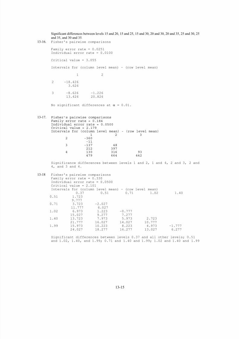
7/12/2019 Solution Manual Stats
http://slidepdf.com/reader/full/solution-manual-stats 471/588
Significant differences between levels 15 and 20, 15 and 25, 15 and 30, 20 and 30, 20 and 35, 25 and 30, 25
and 35, and 30 and 35.
13-16. Fisher's pairwise comparisons
Family error rate = 0.0251Individual error rate = 0.0100
Critical value = 3.055
Intervals for (column level mean) - (row level mean)
1 2
2 -18.4263.626
3 -8.626 -1.22613.426 20.826
No significant differences at α = 0.01.
13-17. Fisher's pairwise comparisons Family error rate = 0.184Individual error rate = 0.0500Critical value = 2.179Intervals for (column level mean) - (row level mean)
1 2 32 -360
-113 -137 48
212 3974 130 316 93
479 664 442
Significance differences between levels 1 and 2, 1 and 4, 2 and 3, 2 and4, and 3 and 4.
13-18 Fisher's pairwise comparisonsFamily error rate = 0.330Individual error rate = 0.0500Critical value = 2.101Intervals for (column level mean) - (row level mean)
0.37 0.51 0.71 1.02 1.400.51 1.723
9.7770.71 3.723 -2.027
11.777 6.0271.02 6.973 1.223 -0.777
15.027 9.277 7.2771.40 13.723 7.973 5.973 2.723
21.777 16.027 14.027 10.7771.99 15.973 10.223 8.223 4.973 -1.777
24.027 18.277 16.277 13.027 6.277
Significant differences between levels 0.37 and all other levels; 0.51and 1.02, 1.40, and 1.99; 0.71 and 1.40 and 1.99; 1.02 and 1.40 and 1.99
13-15

7/12/2019 Solution Manual Stats
http://slidepdf.com/reader/full/solution-manual-stats 472/588
13-19 Fisher's pairwise comparisons
Family error rate = 0.0649Individual error rate = 0.0100Critical value = 2.947Intervals for (column level mean) - (row level mean)
1 2 3 4
2 -8.6428.142
3 5.108 5.35821.892 22.142
4 7.358 7.608 -6.14224.142 24.392 10.642
5 -8.642 -8.392 -22.142 -24.3928.142 8.392 -5.358 -7.608
Significant differences b/t 1 and 3, 1 and 4, 2 and 3, 2 and 4, 3 and 5,4 and 5.
13-20 Fisher's pairwise comparisonsFamily error rate = 0.189Individual error rate = 0.0500Critical value = 2.120Intervals for (column level mean) - (row level mean)
1 2 32 -0.9450
0.94503 1.5550 1.5550
3.4450 3.44504 0.4750 0.4750 -2.0250
2.3650 2.3650 -0.1350
There are significant differences between levels 1 and 3, 4; 2 and 3, 4;and 3 and 4.
13-21. Fisher's pairwise comparisonsFamily error rate = 0.118Individual error rate = 0.0500Critical value = 2.080Intervals for (column level mean) - (row level mean)
1 22 1.799
19.7013 8.424 -2.326
26.326 15.576
Significant differences between levels 1 and 2; and 1 and 3.
13-22.
a) 1952.06
0274.02042.2
225,025.0 =
×==
b
MSt LSD E
Fisher 95% Individual Confidence IntervalsAll Pairwise Comparisons among Levels of Cross-linker level
Simultaneous confidence level = 65.64%
Cross-linker level = -0.5 subtracted from:
Cross-linker
13-16

7/12/2019 Solution Manual Stats
http://slidepdf.com/reader/full/solution-manual-stats 473/588
level Lower Center Upper-0.75 -0.5451 -0.3500 -0.1549-1 -0.7451 -0.5500 -0.35490 -0.1118 0.0833 0.27850.5 0.0215 0.2167 0.41181 -0.1451 0.0500 0.2451
Cross-linker
level ---------+---------+---------+---------+-0.75 (---*---)-1 (---*---)0 (---*---)0.5 (---*---)1 (---*---)
---------+---------+---------+---------+-0.50 0.00 0.50 1.00
Cross-linker level = -0.75 subtracted from:
Cross-linkerlevel Lower Center Upper-1 -0.3951 -0.2000 -0.00490 0.2382 0.4333 0.6285
0.5 0.3715 0.5667 0.76181 0.2049 0.4000 0.5951
Cross-linkerlevel ---------+---------+---------+---------+-1 (---*---)0 (---*---)0.5 (---*---)1 (---*---)
---------+---------+---------+---------+-0.50 0.00 0.50 1.00
Cross-linker level = -1 subtracted from:
Cross-linker
level Lower Center Upper ---------+---------+---------+---------+0 0.4382 0.6333 0.8285 (---*---)0.5 0.5715 0.7667 0.9618 (---*---)1 0.4049 0.6000 0.7951 (---*---)
---------+---------+---------+---------+-0.50 0.00 0.50 1.00
Cross-linker level = 0 subtracted from:
Cross-linkerlevel Lower Center Upper0.5 -0.0618 0.1333 0.32851 -0.2285 -0.0333 0.1618
Cross-linker
level ---------+---------+---------+---------+0.5 (---*---)1 (---*---)
---------+---------+---------+---------+-0.50 0.00 0.50 1.00
Cross-linker level = 0.5 subtracted from:
Cross-linkerlevel Lower Center Upper
13-17

7/12/2019 Solution Manual Stats
http://slidepdf.com/reader/full/solution-manual-stats 474/588
1 -0.3618 -0.1667 0.0285
Cross-linkerlevel ---------+---------+---------+---------+1 (---*---)
---------+---------+---------+---------+-0.50 0.00 0.50 1.00
Cross-linker levels -0.5, 0, 0.5 and 1 do not differ. Cross-linker levels -0.75 and -1 do not differ from one other but both are significantly different to the others.
b) The mean values are
8.0667, 8.2667, 8.6167, 8.7, 8.8333, 8.6667
0676.06
0274.0ˆ ===
b
MS E
X σ
The width of a scaled normal distribution is 6(0.0676) = 0.405
0
0.2
0.4
0.6
0.8
1
8 8.2 8.4 8.6 8.8 9
With a scaled normal distribution over this plot, the conclusions are similar to those from the LSD
method.
13-23.
a) There is no significant difference in protein content between the three diet types.
Fisher 99% Individual Confidence IntervalsAll Pairwise Comparisons among Levels of C4
Simultaneous confidence level = 97.33%
C4 = Barley subtracted from:
C4 Lower Center UpperBarley+lupins -0.3207 -0.0249 0.2709lupins -0.4218 -0.1260 0.1698
C4 -------+---------+---------+---------+--
Barley+lupins (-----------*-----------)lupins (-----------*-----------)
-------+---------+---------+---------+---0.25 0.00 0.25 0.50
C4 = Barley+lupins subtracted from:
C4 Lower Center Upper -------+---------+---------+---------+--lupins -0.3911 -0.1011 0.1889 (-----------*-----------)
-------+---------+---------+---------+--
13-18

7/12/2019 Solution Manual Stats
http://slidepdf.com/reader/full/solution-manual-stats 475/588
-0.25 0.00 0.25 0.50
b) The mean values are: 3.886, 3.8611, 3.76 (barley, b+l, lupins)
From the ANOVA the estimate of σ can be obtainedSource DF SS MS F P
C4 2 0.235 0.118 0.72 0.489 Error 76 12.364 0.163 Total 78 12.599
S = 0.4033 R-Sq = 1.87% R-Sq(adj) = 0.00%The minimum sample size could be used to calculate the standard error ofa sample mean
081.025
163.0ˆ ===
b
MS E
X σ
The graph would not show any differences between the diets.
13-24. 55=μ , τ1 = -5, τ2 = 5, τ3 = -5, τ4 = 5.
)1(4)1(31,)25(4
)100(2
−=−=−==Φ nnaan
n
Various choices for n yield:
n Φ2
Φ a(n-1) Power=1-β
4 4 2 12 0.80
5 5 2.24 16 0.90
Therefore, n = 5 is needed.
13-25 188=μ , τ1 = -13, τ2 = 2, τ3 = -28, τ4 = 12, τ5 = 27.
)1(5)1(41,)100(5
)1830(2 −=−=−==Φ nnaann
Various choices for n yield:n Φ
2Φ a(n-1) Power=1-β
2 7.32 2.7 5 0.55
3 10.98 3.13 10 0.95
Therefore, n = 3 is needed.

7/12/2019 Solution Manual Stats
http://slidepdf.com/reader/full/solution-manual-stats 476/588
, .Section 13-3
13-26 a) Analysis of Variance for UNIFORMITYSource DF SS MS F PWAFERPOS 3 16.220 5.407 8.29 0.008Error 8 5.217 0.652Total 11 21.437
Reject H0, and conclude that there are significant differences among wafer positions.
b) 585.13
652.0407.5ˆ 2 =
−=
−=
n
MS MS E Treatments
τ σ
c) 652.0ˆ 2 == E MSσ
d) Greater variability at wafer position 1. There is some slight curvature in the normal probability plot.
13-19

7/12/2019 Solution Manual Stats
http://slidepdf.com/reader/full/solution-manual-stats 477/588
4321
1
0
-1
WAFERPOS
R e s i d u a l
Residuals Versus WAFERPOS(response is UNIFORMI)
4321
1
0
-1
FittedValue
R e s i d u a l
Residuals Versus the Fitted Values(response is UNIFORMI)
-1 0 1
-2
-1
0
1
2
N o r m a l S c o r e
Residual
Normal Probability Plot of the Residuals(response is uniformi)
13-27 a) Analysis of Variance for OUTPUT
Source DF SS MS F P
LOOM 4 0.3416 0.0854 5.77 0.003
Error 20 0.2960 0.0148
Total 24 0.6376
Reject H0, there are significant differences among the looms.
b) 01412.05
0148.00854.0ˆ 2 =−=−=n
MS MS E Treatments
τ σ
c) 0148.0ˆ 2 == E MSσ
d) Residuals are acceptable
54321
0.2
0.1
0.0
-0.1
-0.2
LOOM
R e s i d u a l
ResidualsVersusLOOM(response is OUTPUT)
4.14.03.93.8
0.2
0.1
0.0
-0.1
-0.2
FittedValue
R e s i d u a l
Residuals Versus the Fitted Values(response is OUTPUT)
13-20

7/12/2019 Solution Manual Stats
http://slidepdf.com/reader/full/solution-manual-stats 478/588
-0.2 -0.1 0.0 0.1 0.2
-2
-1
0
1
2
N o r m a l S c o r e
Residual
Normal Probability Plot of the Residuals(response is OUTPUT)
13-28. a) Yes, the different batches of raw material significantly affect mean yield at α = 0.01 because p-
value is small.
Source DF SS MS F PBatch 5 56358 11272 4.60 0.004
Error 24 58830 2451
Total 29 115188
b) Variability between batches
2.17645
245111272ˆ 2 =
−=
−=
n
MS MS E Treatmentsτ
σ
c) Variability within batches 2451ˆ 2 == MSE σ
d) The normal probability plot and the residual plots show that the model assumptions are
reasonable.
13-21

7/12/2019 Solution Manual Stats
http://slidepdf.com/reader/full/solution-manual-stats 479/588
Residual
P e r c e
n t
100500-50-100
99
90
50
10
1
Fitted Value
R e s i d u
a l
160015501500
100
50
0
-50
-100
Residual
F r
e q u e n c y
1007550250-25-50-75
8
6
4
2
0
Observation Order
R
e s i d u a l
30282624222018161412108642
100
50
0
-50
-100
No rm al Pr ob ab ilit y Plo t o f t h e Resid uals Resid uals Ver su s t h e Fit t ed Valu es
Hist ogram of t he Residuals Residuals Versus t he Order of t he Dat a
Residual Plots for Yield
13-29. a) Analysis of Variance for BRIGHTNENESS
Source DF SS MS F PCHEMICAL 3 54.0 18.0 0.75 0.538Error 16 384.0 24.0Total 19 438.0
Do not reject H0, there is no significant difference among the chemical types.
b) 2.15
0.240.18ˆ 2 −=−=τ σ set equal to 0
c) 0.24ˆ 2 =σ
d) Variability is smaller in chemical 4. There is some curvature in the normal probability plot.
4321
10
5
0
-5
CHEMICAL
R e s i d u a l
Residuals Versus CHEMICAL(response is BRIGHTNE)
8281807978
10
5
0
-5
FittedValue
R e s i d u a l
Residuals Versus the Fitted Values(response is BRIGHTNE)
13-22

7/12/2019 Solution Manual Stats
http://slidepdf.com/reader/full/solution-manual-stats 480/588
1050-5
2
1
0
-1
-2
N o r m a
l S c o r e
Residual
Normal Probability Plot of the Residuals(response is BRIGHTNE)
13-30 a) 237.2ˆˆˆ 222 =+= σ σ σ positiontotal
b) 709.0ˆ
ˆ
2
2
=total
position
σ
σ
c) It could be reduced to 0.6522. This is a reduction of approximately 71%.
13-31.
a) Instead of testing the hypothesis that the individual treatment effects are zero, we are testing
whether there is variability in protein content between all diets.
0:
0:
2
1
2
0
≠
=
τ
τ
σ
σ
H
H
b) The statistical model is
⎩⎨⎧
=
=++=
n j
ai y iji
,...,2,1
,...,2,1ε τ μ
and),0(~ 2σ ε N i ),0(~ 2τ
σ τ N i
c)
The last TWO observations were omitted from two diets to generate equal sample sizes with n = 25.
ANOVA: Protein versus DietTypeAnalysis of Variance for Protein
Source DF SS MS F P
DietType 2 0.2689 0.1345 0.82 0.445
Error 72 11.8169 0.1641
Total 74 12.0858
S = 0.405122 R-Sq = 2.23% R-Sq(adj) = 0.00%
1641.02 == E MSσ
001184.025
1641.01345.02 −=−
=−
=n
MS MS E tr
τ σ
13-23

7/12/2019 Solution Manual Stats
http://slidepdf.com/reader/full/solution-manual-stats 481/588
Section 13-4
13-32.
a) Analysis of variance for GlucoseSource DF SS MS F P
Time 1 36.13 36.125 0.06 0.819
Min 1 128.00 128.000 0.21 0.669
Error 5 3108.75 621.750Total 7 3272.88
No, there is no effect of exercise time on the average blood glucose.
b) P-value = 0.819
c) The normal probability plot and the residual plots show that the model assumptions are
reasonable.
Residual
P e r c e n t
50250-25-50
99
90
50
10
1
Fitted Value
R e s i d u a l
110105100
20
0
-20
-40
Residual
F r e q u e n c y
20100-10-20-30-40
3
2
1
0
Observation Order
R e s i d u a l
87654321
20
0
-20
-40
No rm al Pr ob ab ilit y Plo t o f t h e Resid uals Resid uals Ver su s t h e Fit t ed Valu es
Hist o gram of t h e Resid uals Resid uals Versus t h e Order of t h e Dat a
Residual Plot s for Glucose
13-33. a) Analysis of Variance for SHAPE
Source DF SS MS F PNOZZLE 4 0.102180 0.025545 8.92 0.000VELOCITY 5 0.062867 0.012573 4.39 0.007
Error 20 0.057300 0.002865Total 29 0.222347
Reject H0, nozzle type affects shape measurement.
13-24

7/12/2019 Solution Manual Stats
http://slidepdf.com/reader/full/solution-manual-stats 482/588
28.7423.4620.4316.5914.3711.73
1.15
1.05
0.95
0.85
0.75
VELOCITY
S
H A P E
54321
1.15
1.05
0.95
0.85
0.75
NOZZLE
S H A P E
b) Fisher's pairwise comparisons
Family error rate = 0.268
Individual error rate = 0.0500
Critical value = 2.060
Intervals for (column level mean) - (row level mean)
1 2 3 4
2 -0.15412
0.01079
3 -0.20246 -0.13079
-0.03754 0.034124 -0.24412 -0.17246 -0.12412
-0.07921 -0.00754 0.04079
5 -0.11412 -0.04246 0.00588 0.04754
0.05079 0.12246 0.17079 0.21246
There are significant differences between levels 1 and 3, 4; 2 and 4; 3
and 5; and 4 and 5.
c) The residual analysis shows that there is some inequality of variance. The normal probability plot is
acceptable.
302010
0.1
0.0
-0.1
VELOCITY
R e s i d u a l
Residuals Versus VELOCITY(response is SHAPE)
54321
0.1
0.0
-0.1
NOZZLE
R e s i d u a l
Residuals Versus NOZZLE(response is SHAPE)
13-25
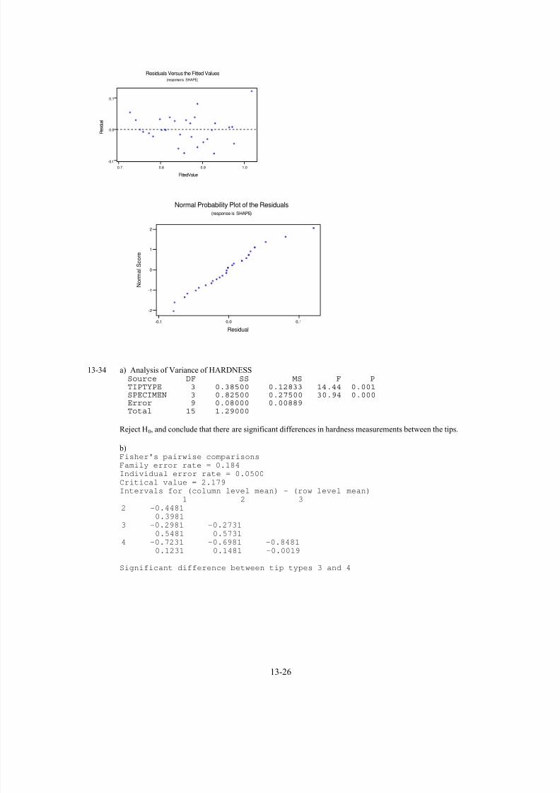
7/12/2019 Solution Manual Stats
http://slidepdf.com/reader/full/solution-manual-stats 483/588
1.00.90.80.7
0.1
0.0
-0.1
FittedValue
R e s i d u a l
Residuals Versus the Fitted Values(response is SHAPE)
0.10.0-0.1
2
1
0
-1
-2
N o r m a l S c o r e
Residual
Normal Probability Plot of the Residuals(response is SHAPE)
13-34 a) Analysis of Variance of HARDNESSSource DF SS MS F PTIPTYPE 3 0.38500 0.12833 14.44 0.001SPECIMEN 3 0.82500 0.27500 30.94 0.000Error 9 0.08000 0.00889
Total 15 1.29000
Reject H0, and conclude that there are significant differences in hardness measurements between the tips.
b)Fisher's pairwise comparisons
Family error rate = 0.184
Individual error rate = 0.0500
Critical value = 2.179
Intervals for (column level mean) - (row level mean)
1 2 3
2 -0.4481
0.3981
3 -0.2981 -0.2731
0.5481 0.5731
4 -0.7231 -0.6981 -0.8481
0.1231 0.1481 -0.0019
Significant difference between tip types 3 and 4
13-26

7/12/2019 Solution Manual Stats
http://slidepdf.com/reader/full/solution-manual-stats 484/588
c) Residuals are acceptable.
4321
0.15
0.10
0.05
0.00
-0.05
-0.10
SPECIMEN
R e s i d u a l
Residuals Versus SPECIMEN(response is HARDNESS)
4321
0.15
0.10
0.05
0.00
-0.05
-0.10
TIPTYPE
R e s i d u a l
Residuals Versus TIPTYPE(response is HARDNESS)
10.210.110.09.99.89.79.69.59.49.39.2
0.15
0.10
0.05
0.00
-0.05
-0.10
FittedValue
R e s i d u a l
Residual s Versus the Fitted Values(response is HARDNESS)
-0.10 -0.05 0.00 0.05 0.10 0.15
-2
-1
0
1
2
N o r m a l S c o r e
Residual
Normal Probability Plot of the Residuals(response is hardness)
13-35. a) Analysis of Variance for ARSENIC
Source DF SS MS F PTEST 2 0.0014000 0.0007000 3.00 0.125SUBJECT 3 0.0212250 0.0070750 30.32 0.001
Error 6 0.0014000 0.0002333Total 11 0.0240250
Do not reject H0, there is no evidence of differences between the tests.
13-27
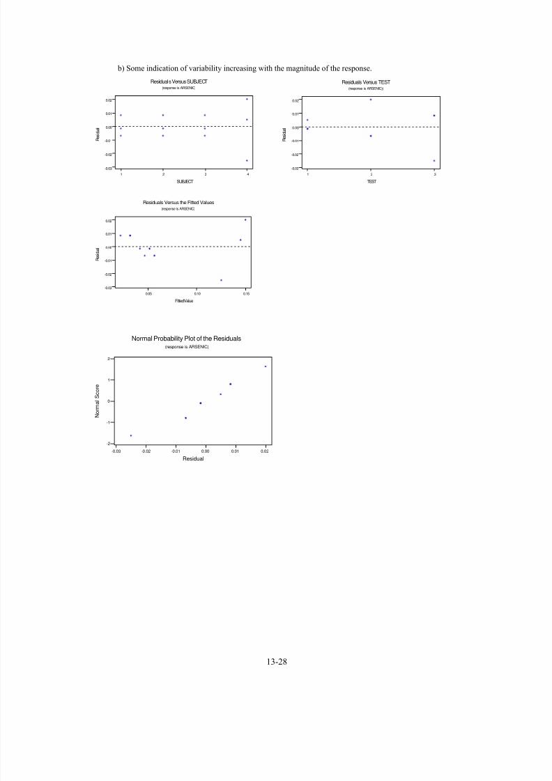
7/12/2019 Solution Manual Stats
http://slidepdf.com/reader/full/solution-manual-stats 485/588
b) Some indication of variability increasing with the magnitude of the response.
4321
0.02
0.01
0.00
-0.01
-0.02
-0.03
SUBJECT
R e s i d u a l
Residuals Versus SUBJECT(response is ARSENIC)
321
0.02
0.01
0.00
-0.01
-0.02
-0.03
TEST
R e s i d u a l
Residuals Versus TEST(response is ARSENIC))
0.150.100.05
0.02
0.01
0.00
-0.01
-0.02
-0.03
FittedValue
R e s i d u a l
Residuals Versus the Fitted Values(response is ARSENIC)
-0.03 -0.02 -0.01 0.00 0.01 0.02
-2
-1
0
1
2
N o r m a
l S c o r e
Residual
Normal Probability Plot of the Residuals(response is ARSENIC)
13-28

7/12/2019 Solution Manual Stats
http://slidepdf.com/reader/full/solution-manual-stats 486/588
13-36. a) Analysis of Variance of PROPECTINSource DF SS MS F PSTORAGE 3 1972652 657551 4.33 0.014LOT 8 1980499 247562 1.63 0.169Error 24 3647150 151965Total 35 7600300
Reject H0, and conclude that the storage times affect the mean level of propectin.
b) P-value = 0.014
c)Fisher's pairwise comparisons
Family error rate = 0.196
Individual error rate = 0.0500
Critical value = 2.037
Intervals for (column level mean) - (row level mean)
0 7 14
7 -171
634
14 -214 -445
592 360
21 239 8 50
1045 813 856
There are differences between 0 and 21 days; 7 and 21 days; and 14 and 21 days. The propectin levels are
significantly different at 21 days from the other storage times so there is evidence that the mean level of
propectin decreases with storage time. However, differences such as between 0 and 7 days and 7 and 14 days
were not significant so that the level is not simply a linear function of storage days.
d) Observations from lot 3 at 14 days appear unusual. Otherwise, the residuals are acceptable.
10005000-500
2
1
0
-1
-2
N o r m a l S c o r e
Residual
Normal Probability Plot of the Residuals(response is propecti)
9876543210
1000
500
0
-500
LOT
R e s i d u a l
Residuals Versus LOT(response is PROTOPE)
20100
1000
500
0
-500
STORAGE
R e s i d u a l
ResidualsVersusSTORAGE(response is PROTOPEC)
13-29

7/12/2019 Solution Manual Stats
http://slidepdf.com/reader/full/solution-manual-stats 487/588
150010005000
1000
500
0
-500
Fitted Value
R e s i d u a l
Residual s Versus the Fitted Va lues(response is PROTOPEC)
13-37. A version of the electronic data file has the reading for length 4 and width 5 as 2. It should be 20.
a) Analysis of Variance for LEAKAGE
Source DF SS MS F PLENGTH 3 72.66 24.22 1.61 0.240WIDTH 4 90.52 22.63 1.50 0.263Error 12 180.83 15.07Total 19 344.01
Do not reject H0, mean leakage voltage does not depend on the channel length.
b) One unusual observation in width 5, length 4. There are some problems with the normal probability plot,
including the unusual observation.
54321
10
5
0
WIDTH
R e s i d u a l
Residuals Versus WIDTH(response is LEAKAGE)
1050
10
5
0
FittedValue
R e s i d u a l
Residuals Versus the Fitted Values(response is LEAKAGE)
0 5 10
-2
-1
0
1
2
N o r m a l S c o r e
Residual
Normal Probability Plot of the Residuals(response is LEAKAGE)
4321
10
5
0
LENGTH
R e s i d u a l
Residuals Versus LENGTH(response is LEAKAGE)
13-30

7/12/2019 Solution Manual Stats
http://slidepdf.com/reader/full/solution-manual-stats 488/588
c) Analysis of Variance for LEAKAGE VOLTAGESource DF SS MS F PLENGTH 3 8.1775 2.7258 6.16 0.009WIDTH 4 6.8380 1.7095 3.86 0.031Error 12 5.3100 0.4425Total 19 20.3255
Reject H0. And conclude that the mean leakage voltage does depend on channel length. By removing the
data point that was erroneous, the analysis results in a conclusion. The erroneous data point that was anobvious outlier had a strong effect the results of the experiment.

7/12/2019 Solution Manual Stats
http://slidepdf.com/reader/full/solution-manual-stats 489/588
Supplemental Exercises
13-38 a) Analysis of Variance for SURFACE ROUGNESSAnalysis of Variance for y
Source DF SS MS F P
Material 3 0.2402 0.0801 4.96 0.020
Error 11 0.1775 0.0161
Total 14 0.4177
Reject H0
b) One observation is an outlier.
1 2 3 4
-0.2
-0.1
0.0
0.1
0.2
0.3
Material
R e s i d u a l
Residuals Versus Material
(response is Surf Rou)
13-31

7/12/2019 Solution Manual Stats
http://slidepdf.com/reader/full/solution-manual-stats 490/588
-0.2 -0.1 0.0 0.1 0.2 0.3
-2
-1
0
1
2
N o r m a l S c o r e
Residual
Normal Probability Plot of the Residuals
(response is Surf Rou)
c) There appears to be a problem with constant variance. This may be due to the outlier in the data.
0.1 0.2 0.3 0.4 0.5
-0.2
-0.1
0.0
0.1
0.2
0.3
Fitted Value
R e s i d u a l
Residuals Versus the Fitted Values(response is Surf Rou)
d) 95% confidence interval on the difference in the means of EC10 and EC1
602.0118.0
2
)0161.0(
4
)0161.0(201.2)130.0490.0(
2
)0161.0(
4
)0161.0(201.2)130.0490.0(
41
41
21
11,,025.04131
21
11,,025.041
≤−≤
++−≤−≤+−−
++−≤−≤+−−
μ μ
μ μ
μ μ n
MS
n
MSt y y
n
MS
n
MSt y y E E E E
13-39. a) Analysis of Variance for RESISTANCESource DF SS MS F P ALLOY 2 10941.8 5470.9 76.09 0.000Error 27 1941.4 71.9Total 29 12883.2
Reject H0, the type of alloy has a significant effect on mean contact resistance.
13-32

7/12/2019 Solution Manual Stats
http://slidepdf.com/reader/full/solution-manual-stats 491/588
b) Fisher's pairwise comparisonsFamily error rate = 0.119
Individual error rate = 0.0500
Critical value = 2.052
Intervals for (column level mean) - (row level mean)
1 2
2 -13.58
1.98
3 -50.88 -45.08-35.32 -29.52
There are differences in the mean resistance for alloy types 1 and 3; and types 2 and 3.
c) 99% confidence interval on the mean contact resistance for alloy 3
83.14797.132
10
9.71771.24.140
10
9.71771.24.140
1
3
27,005.0327,005.03
≤≤
+≤≤−
+≤≤−
μ
μ
μ n
MSt y
n
MSt y E
i
E
d) Variability of the residuals increases with the response. The normal probability plot has some
curvature in the tails, indicating a problem with the normality assumption. A transformation of the
response should be conducted.
321
30
20
10
0
-10
-20
ALLOY
R e s i d u a l
Residuals VersusALLOY(response is RESISTAN))
140130120110100
30
20
10
0
-10
-20
FittedValue
R e s i d u a l
Residuals Versus the Fitted Values(response is RESISTAN)
-20 -10 0 10 20 30
-2
-1
0
1
2
N o r m a l S c o r e
Residual
Normal Probability Plot of the Residuals(response is RESISTAN)
13-33

7/12/2019 Solution Manual Stats
http://slidepdf.com/reader/full/solution-manual-stats 492/588
13-40 a) Analysis of Variance for SCORESource DF SS MS F PMETHOD 2 13.55 6.78 1.68 0.211Error 21 84.77 4.04Total 23 98.32
Do not reject H0
b) P-value = 0.211
c) There is some curvature in the normal probability plot. There appears to be some differences in the
variability for the different methods. The variability for method one is larger than the variability for method
3.
3210-1-2-3-4-5
2
1
0
-1
-2
N o r m a l S c o r e
Residual
Normal Probability Plot of the Residuals(response is score)
321
3
2
1
0
-1
-2
-3
-4
-5
METHOD
R e s i d u a l
Residuals Versus METHOD(response is SCORE)
d.) 342.08
04.478.6ˆ 2 =
−=
−=
n
MS MS E Treatments
τ σ
04.4ˆ 2 == E MSσ
13-41. a) Analysis of Variance for VOLUMESource DF SS MS F PTEMPERATURE 2 16480 8240 7.84 0.007Error 12 12610 1051
Total 14 29090Reject H0.
b) P-value = 0.007
c) Fisher's pairwise comparisonsFamily error rate = 0.116
Individual error rate = 0.0500
Critical value = 2.179
Intervals for (column level mean) - (row level mean)
70 75
13-34

7/12/2019 Solution Manual Stats
http://slidepdf.com/reader/full/solution-manual-stats 493/588
75 -16.7
72.7
80 35.3 7.3
124.7 96.7
There are significant differences in the mean volume for temperature levels 70 and 80; and 75 and 80. The
highest temperature results in the smallest mean volume.
d) There are some relatively small differences in the variability at the different levels of temperature. The
variability decreases with the fitted values. There is an unusual observation on the normal probability plot.
-50 0 50
-2
-1
0
1
2
N o r m a l S c o r e
Residual
Normal Probability Plot of the Residuals(response is vol)
807570
50
0
-50
TEMPERAT
R e s i d u a l
Residuals Versus TEMPERAT(response is VOLUME)
125012401230122012101200119011801170
50
0
-50
FittedValue
R e s i d u a l
Residuals Versus the Fitted Values(response is VOLUME)
13-42. a)Analysis of Variance of Weight GainSource DF SS MS F PMEANWEIG 2 0.2227 0.1113 1.48 0.273 AIRTEMP 5 10.1852 2.0370 27.13 0.000Error 10 0.7509 0.0751Total 17 11.1588
Reject H0 and conclude that the air temperature has an effect on the mean weight gain.
b) Fisher's pairwise comparisonsFamily error rate = 0.314
Individual error rate = 0.0500
Critical value = 2.179Intervals for (column level mean) - (row level mean)
50 60 70 80 90
60 -0.9101
0.1034
70 -1.2901 -0.8868
-0.2766 0.1268
80 -0.9834 -0.5801 -0.2001
0.0301 0.4334 0.8134
90 -0.3034 0.0999 0.4799 0.1732
0.7101 1.1134 1.4934 1.1868
100 1.0266 1.4299 1.8099 1.5032 0.8232
13-35

7/12/2019 Solution Manual Stats
http://slidepdf.com/reader/full/solution-manual-stats 494/588
2.0401 2.4434 2.8234 2.5168 1.8368
There are significant differences in the mean air temperature levels 50
and 70, 100; 60 and 90, 100; 70 and 90, 100; 80 and 90, 100; and 90 and
100. The mean of temperature level 100 is different from all the other
temperatures.
c) There appears to be some problems with the assumption of constant variance.
200150100
0.5
0.0
-0.5
MEANWEIG
R e s i d u a l
Residuals Versus MEANWEIG(response is WEIGHTGA)
1009080706050
0.5
0.0
-0.5
AIRTEMP
R e s i d u a l
Residuals Versus AIRTEMP(response is WEIGHTGA)
210
0.5
0.0
-0.5
FittedValue
R e s i d u a l
Residuals Versusthe Fitted Values(response is WEIGHTGA)
0.50.0-0.5
2
1
0
-1
-2
N o r m a l S c o r e
Residual
Normal Probability Plot of the Residuals(response is wt gain)
13-43. a) Analysis of Variance for PCTERROR
Source DF SS MS F P ALGORITH 5 2825746 565149 6.23 0.000PROJECT 7 2710323 387189 4.27 0.002Error 35 3175290 90723Total 47 8711358
13-36
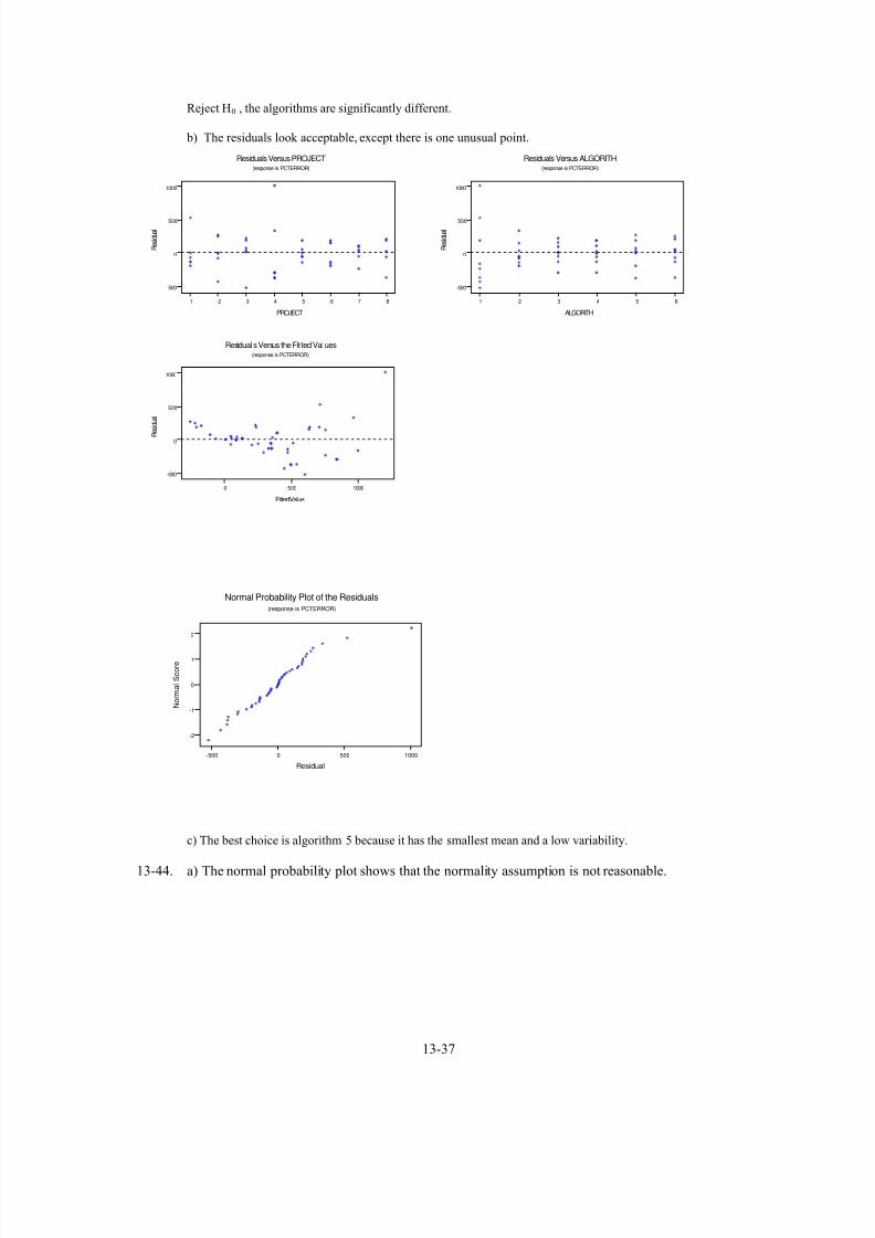
7/12/2019 Solution Manual Stats
http://slidepdf.com/reader/full/solution-manual-stats 495/588
Reject H0 , the algorithms are significantly different.
b) The residuals look acceptable, except there is one unusual point.
87654321
1000
500
0
-500
PROJECT
R e s i d u a l
Residuals Versus PROJECT(response is PCTERROR)
654321
1000
500
0
-500
ALGORITH
R e s i d u a l
Residuals Versus ALGORITH(response is PCTERROR)
10005000
1000
500
0
-500
FittedValue
R e s i d u a l
Residuals Versus the Fit ted Values(response is PCTERROR)
10005000-500
2
1
0
-1
-2
N o r m a l S c o r e
Residual
Normal Probability Plot of the Residuals(response is PCTERROR)
c) The best choice is algorithm 5 because it has the smallest mean and a low variability.
13-44. a) The normal probability plot shows that the normality assumption is not reasonable.
13-37

7/12/2019 Solution Manual Stats
http://slidepdf.com/reader/full/solution-manual-stats 496/588
Obs
P e r c e n t
150010005000-500
99
95
90
80
70
60
50
40
30
20
10
5
1
Mean
<0.005
293.8
StDev 309.4
N 3
A D 2.380
P-Value
Probabilit y Plot of ObsNormal - 95% CI
0
b) The normal probability plot shows that the normality assumption is reasonable.
log(obs)
P e r c e n t
4.03.53.02.52.01.51.00.5
99
95
90
80
70
60
50
40
30
20
10
5
1
Mean
0.066
2.209StDev 0.5060
N 30
A D 0.687
P-Value
Probabilit y Plot of l og(obs)Normal - 95% CI
Source DF SS MS F P
Treatments 2 1.188 0.594 2.57 0.095Error 27 6.237 0.231
Total 29 7.425
There is evidence to support the claim that the treatment means differ at α = 0.1 for the
transformed data since the P-value = 0.095.
c) The normal probability plot and the residual plots show that the model assumptions are
reasonable.
13-38

7/12/2019 Solution Manual Stats
http://slidepdf.com/reader/full/solution-manual-stats 497/588
Residual
P e r c e
n t
1.00.50.0-0.5-1.0
99
90
50
10
1
Fitted Value
R e s i d u
a l
2.52.42.32.22.1
1.0
0.5
0.0
-0.5
-1.0
Residual
F r
e q u e n c y
0.80.40.0-0.4-0.8
8
6
4
2
0
Observation Order
R
e s i d u a l
30282624222018161412108642
1.0
0.5
0.0
-0.5
-1.0
No rm al Pr ob ab ilit y Plo t o f t h e Resid uals Resid uals Ver su s t h e Fit t ed Valu es
Hist ogram of t he Residuals Residuals Versus t he Order of t he Dat a
Residual Plots for log( obs)
13-45. a) μ=1.6, =0.284, =0.5333 2Φ Φ
Numerator degrees of freedom = 141 ν ==−a
Denominator degrees of freedom =215)1( ν ==−na
From Chart Figure 13-6, β ≈0.8 and the power = 1 - β = 0.2
b)
n Φ2 Φ a(n-1) β Power = 1-β
50 3.56 1.89 245 0.05 0.95
The sample size should be approximately n = 50.
13-46. a) μ = (1+5+8+4)/4 = 4.5 and
5.2
25.6)4(4
])5.44()5.48()5.45()5.41[(4 22222
=Φ
=−+−+−+−
=Φ
Numerator degrees of freedom = 131 ν ==−a
Denominator degrees of freedom =212)1( ν ==−na
From Figure 13-6, β = 0.05 and the power = 1 - β = 0.95
b)
n Φ2
Φ a(n-1) β Power = 1-β
4 6.25 2.5 12 0.05 0.95
3 4.6875 2.165 8 0.25 0.75
The sample size should be approximately n = 4.
13-39

7/12/2019 Solution Manual Stats
http://slidepdf.com/reader/full/solution-manual-stats 498/588
13-40
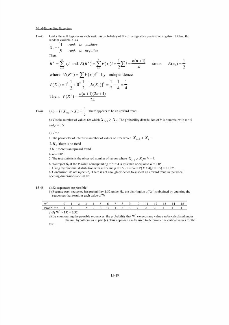
7/12/2019 Solution Manual Stats
http://slidepdf.com/reader/full/solution-manual-stats 499/588
Mind-Expanding Exercises
15-43 Under the null hypothesis each rank has probability of 0.5 of being either positive or negative. Define the
random variable Xi as
⎩⎨⎧
=negativeisrank
positiveisrank X i
0
1
Then,
24
)12)(1()( Then,
4
1
4
1
2
1)]([
2
10
2
11)(
ceindependen by )()( where
2
1)(since
4
)1(
2
1)()( and
222
2
11
++=
=−=−+=
=
=+
====
+
+
=
+
=
+
∑
∑∑∑
nnn RV
X E X V
i xV RV
x E nn
ii x E R E i x R
ii
i
i
n
i
i
n
i
i
15-44 a) 5
4
)( 5=>= + ii X X P p There appears to be an upward trend.
b) V is the number of values for which . The probability distribution of V is binomial with n = 5
and p = 0.5.
ii X X >+5
c) V = 4
1. The parameter of interest is number of values of i for which .ii X X >+5
trendupwardanisthere:3
trendnoisthere:.2
1
0
H
H
4. α = 0.05
5. The test statistic is the observed number of values where or V = 4.ii X X >+5
6. We reject H 0 if the P-value corresponding to V = 4 is less than or equal to α = 0.05.
7. Using the binomial distribution with n = 5 and p = 0.5, P-value = P( V ≥ 4| p = 0.5) = 0.18758. Conclusion: do not reject H 0. There is not enough evidence to suspect an upward trend in the wheel
opening dimensions at α=0.05.
15-45 a) 32 sequences are possible
b) Because each sequence has probability 1/32 under H0, the distribution of W*
is obtained by counting the
sequences that result in each value of W*
w* 0 1 2 3 4 5 6 7 8 9 10 11 12 13 14 15
Prob*1/32 1 1 1 2 2 3 3 3 3 3 3 2 2 1 1 1
c) P( W* > 13) = 2/32
d) By enumerating the possible sequences, the probability that W* exceeds any value can be calculated under
the null hypothesis as in part (c). This approach can be used to determine the critical values for the
test.
15-19

7/12/2019 Solution Manual Stats
http://slidepdf.com/reader/full/solution-manual-stats 500/588
CHAPTER 15
Section 15-2
15-1 a)
1. The parameter of interest is median of pH.
0.7~:3
0.7~:.2
1
0
≠
=
μ
μ
H
H
4. α=0.05
5. The test statistic is the observed number of plus differences or r + = 8.
6. We reject H 0 if the P-value corresponding to r + = 8 is less than or equal to α = 0.05.
7. Using the binomial distribution with n = 10 and p = 0.5, P-value = 2P(R + ≥ 8 | p = 0.5) = 0.1
8. Conclusion: we cannot reject H 0. There is not enough evidence to reject the manufacturer’s claim that the
median of the pH is 7.0
b)
1. The parameter of interest is median of pH.
0.7~:3
0.7~:.2
1
0
≠
=
μ
μ
H
H
4. α=0.05
5. The test statistic isn
nr z
5.0
5.0*
0−=
6. We reject H 0 if |Z0|>1.96 for α=0.05.
7. r*=8 and 90.1105.0
)10(5.08
5.0
5.0*
0 =−
=−
=n
nr z
8. Conclusion: we cannot reject H 0. There is not enough evidence to reject the manufacturer’s claim that
the median of the pH is 7.0
P-value = 2[1 - P(|Z0| < 1.90)] = 2(0.0287) = 0.0574
15-2 a)
1. The parameter of interest is median titanium content.
5.8~:3
5.8~:.2
1
0
≠=
μ
μ
H
H
4. α=0.05
5. The test statistic is the observed number of plus differences or r +
= 7.
6. We reject H 0 if the P-value corresponding to r + = 7 is less than or equal to α=0.05.
7. Using the binomial distribution with n=10 and p=0.5, P-value = 2P(R *≤7|p=0.5)=0.359
8. Conclusion: we cannot reject H 0. There is not enough evidence to reject the manufacturer’s claim that
the median of the titanium content is 8.5.
b)
1. Parameter of interest is the median titanium content
5.8~:.3
5.8~:.2
1
0
≠
=
μ
μ
H
H
4. α=0.05
5. Test statistic isn
nr z
5.0
5.00
−=
+
6. We reject H 0 if the | Z 0| > Z 0.025 = 1.96
7. Computation: 34.1205.0
)20(5.070 −=
−= z
8. Conclusion, cannot reject H 0. There is not enough evidence to conclude that the median titanium content
differs from 8.5. The P-value = 2*P( | Z | > 1.34) = 0.1802.
15-1

7/12/2019 Solution Manual Stats
http://slidepdf.com/reader/full/solution-manual-stats 501/588
15-3 a)
1. Parameter of interest is the median impurity level.
5.2~:.3
5.2~:.2
1
0
<
=
μ
μ
H
H
4. α=0.05
5. The test statistic is the observed number of plus differences or r + = 2.
6. We reject H 0 if the P-value corresponding to r +
= 2 is less than or equal to α = 0.05.7. Using the binomial distribution with n = 22 and p = 0.5, P-value = P(R +≤ 2 | p = 0.5) = 0.0002
8. Conclusion, reject H 0. The data supports the claim that the median is impurity level is less than 2.5.
b)
1. Parameter of interest is the median impurity level
5.2~:.3
5.2~:.2
1
0
<
=
μ
μ
H
H
4. α=0.05
5. Test statistic isn
nr z
5.0
5.00
−=
+
6. We reject H 0 if the Z 0 < Z 0.05 = -1.65
7. Computation:84.3225.0
)22(5.020 −=
−
= z
8. Conclusion, reject H 0 and conclude that the median impurity level is less than 2.5. The P-value = P( Z <-
3.84) = 0.000062
15-4 a)
1. Parameter of interest is the median margarine fat content
0.17~:.3
0.17~:.2
1
0
≠
=
μ
μ
H
H
4. α=0.05
5. The test statistic is the observed number of plus differences or r +
= 3.
6. We reject H 0 if the P-value corresponding to r + = 7 is less than or equal to α=0.05.
7. Using the binomial distribution with n=6 and p=0.5, P-value = 2*P(R *≥3|p=0.5,n=6)=1.
8. Conclusion, cannot reject H 0. There is not enough evidence to conclude that the median fat content differs
from 17.0.
b)
1. Parameter of interest is the median margarine fat content
0.17~:.3
0.17~:.2
1
0
≠
=
μ
μ
H
H
4. α=0.05
5. Test statistic is
n
nr z
5.0
5.00
−=
+
6. We reject H 0 if the | Z 0| > Z 0.025 = 1.96
7. Computation: 065.0
)6(5.030 =
−= z
8. Conclusion, cannot reject H 0. The P-value = 1-Φ(0) = 1 – 0.5 = 0.5. There is not enough evidence toconclude that the median fat content differs from 17.0.
15-2

7/12/2019 Solution Manual Stats
http://slidepdf.com/reader/full/solution-manual-stats 502/588
15-5 a)
1. Parameter of interest is the median compressive strength
2250~:.3
2250~:.2
1
0
>
=
μ
μ
H
H
4. α = 0.05
5. The test statistic is the observed number of plus differences or r + = 7.
6. We reject H 0 if the P-value corresponding to r +
= 7 is less than or equal to α=0.05.7. Using the binomial distribution with n = 12 and p = 0.5, P-value = P( R + ≥ 7 | p = 0.5) = 0.3872
8. Conclusion, cannot reject H 0. There is not enough evidence to conclude that the median compressive
strength is greater than 2250.
b)
1. Parameter of interest is the median compressive strength
2250~:.3
2250~:.2
1
0
>
=
μ
μ
H
H
4. α=0.05
5. Test statistic is
n
nr z
5.0
5.00
−=
+
6. We reject H 0 if the | Z 0| > Z 0.025 = 1.96
7. Computation: 577.0125.0
)12(5.070 =−= z
8. Conclusion, cannot reject H 0. The P-value = 1-Φ(0.58) = 1 - 0.7190 = 0.281. There is not enough
evidence to conclude that the median compressive strength is greater than 2250.
15-6 a)
1. Parameters of interest are the median caliper measurements
0~:.3
0~:.2
1
0
≠
=
D
D
H
H
μ
μ
4. α=0.05
5. The test statistic is r = min( r + , r -).
6. Because α =0.05 and n = 12, Appendix A, Table VIII gives the critical value of = 2. We reject*
05.0r
H 0 in favor of H 1 if r ≤ 2.7. There are four ties that are ignored so that r + = 6 and r - = 2 and r = min(6,2) = 2
8. Conclusion, reject H 0. There is a significant difference in the median measurements of the two calipers at
α = 0.05.
b)
1. Parameters of interest are the median caliper measurements
0~:.3
0~:.2
1
0
≠
=
D
D
H
H
μ
μ
4. α=0.05
5. Test statisticn
nr z
5.0
5.00
−=
+
6. We reject H 0 if the | Z 0| > Z 0.025 = 1.96
7. Computation: 41.185.0
)8(5.060 =−= z
8. Conclusion, do not reject H 0. There is not a significant difference in the median measurements of the two
calipers at α = 0.05.
The P-value = 2[1-P( | Z 0| < 1.41) = 0.159.
15-7 a)
15-3

7/12/2019 Solution Manual Stats
http://slidepdf.com/reader/full/solution-manual-stats 503/588
1. Parameters of interest are the median hardness readings for the two tips
0~:.3
0~:.2
1
0
≠
=
D
D
H
H
μ
μ
4. α=0.05
5. The test statistic is r = min( r +, r -).
6. Because α = 0.05 and n = 8, Appendix A, Table VIII gives the critical value of = 0. We reject*
05.0r
H 0 in favor of H 1 if r ≤ 0.
7. r + = 6 and r - = 2 and r = min(6,2) = 2
8. Conclusion, cannot reject H 0. There is not a significant difference in the tips.
b) P-value = 2P(R − ≥ 6 | p = 0.5) = 0.289. The P-value is greater than 0.05, therefore we cannot reject H0
and conclude that there is no significant difference between median hardness readings for the two tips. This
result agrees with the result found in Exercise 15-9.
15-8 a)
1. Parameters of interest are the median drying times for the two formulations
0~:.3
0~:.2
1
0
≠
=
D
D
H
H
μ
μ
4. α=0.01
5. The test statistic is r = min( r +
, r -
).
6. Because α = 0.01 and n = 20, Appendix A, Table VIII gives the critical value of = 3. We reject*
01.0r
H 0 in favor of H 1 if r ≤ 3.
7. There are two ties that are ignored so that r +
= 3 and r - = 15 and r = min(3,15) = 3
8. Conclusion, reject H 0. There is a significant difference in the drying times of the two formulations at α =
0.01.
b)
1. Parameters of interest are the median drying times of the two formulations
0~:.3
0~:.2
1
0
≠
=
D
D
H
H
μ
μ
4. α=0.01
5. Test statisticnnr z
5.05.00 −=
+
6. We reject H 0 if the | Z 0| > Z 0.005 = 2.58
7. Computation: 83.2185.0
)18(5.030 −=
−= z
8. Conclusion, reject H 0 and conclude that there is a significant difference between the drying times for the
two formulations at α = 0.01.
The P-value = 2[1-P( | Z 0| < 2.83) = 0.005.
c) P-value = 2P(R − ≤ 3 | p = 0.5) = 0.0075. The exact P-value computed here agrees with the normal
approximation in Exercise 15-11 in the sense that both calculations would lead to the rejection of H0.
15-9 a) for x > 0. Because 3.5 is the median . Solving for λ, we find λ = 0.198
and E( X ) = 1/λ = 5.05
xe x f λ λ −=)( 5.05.3
0
=−∫xe λ λ
b) Because r * = 3 > 1, do not reject H0
c) β = P(Type II error)=P(R * > 1| =4.5)~μ
15-4

7/12/2019 Solution Manual Stats
http://slidepdf.com/reader/full/solution-manual-stats 504/588
For ~μ = 4.5, E( X ) = 6.49 and P(X < 3.5| =4.5) = 0.4167. Therefore, with~μ =−∫ xe
154.0
5.3
0
154.0
n =10, p = 0.4167, β = P(Type II error)=P(R * > 1| =4.5) = 0.963~μ
15-10 a)
1. Parameters of interest are the median blood cholesterol levels
0~:.3
0~:.2
1
0
≠
=
D
D
H
H
μ
μ
4. α=0.05
5. The test statistic r = min( r + , r -).
6. Because α = 0.05 and n = 15, Appendix A, Table VIII gives the critical value of = 3. We reject*
05.0r
H 0 in favor of H 1 if r ≤ 3.
7. r + = 14 and r - = 1 and r = min(14,1) = 1
8. Conclusion, reject H 0. There a significant difference in the blood cholesterol levels atα = 0.05.
b)
1. Parameter of interest is the difference in blood cholesterol levels
0~:.30
~:.2
1
0
≠=
D
D
H H
μ μ
4. α=0.05
5. Test statisticn
nr z
5.0
5.00
−=
+
6. We reject H 0 if the | Z 0| > Z 0.025 = 1.96
7. Computation: 36.3155.0
)15(5.0140 =
−= z
8. Conclusion, reject H 0. There is a difference between the blood cholesterol levels.
The P-value = 2*P (| Z | > 3.36) = 0.0008.
15-11 a) α = P(Z > 1.96) = 0.025
b) 115.0)20.1(1|96.1/
=−<=⎟⎟ ⎠
⎞⎜⎜⎝
⎛ === Z P
n
X P μ
σ β
c) The sign test that rejects if R − ≤ 1 has α = 0.011 based on the binomial distribution.
d) ( ) 1587.0)1(1|2 =>==≥= − Z P RP μ β . Therefore, R − has a binomial distribution with p =
0.1587 and n = 10 when μ = 1. Then β = 0.487. The value of β is greater for the sign test than for the normal
test because the Z-test was designed for the normal distribution.
15-5

7/12/2019 Solution Manual Stats
http://slidepdf.com/reader/full/solution-manual-stats 505/588
Section 15-3
Note to Instructors: When an observation equals the hypothesized mean the observation is dropped and not
considered in the analysis.
15-12 a)
1. Parameter of interest is the mean titanium content
5.8:.3
5.8:.2
1
0
≠
=
μ
μ
H
H
4. α=0.05
5. The test statistic is w = min( w + , w -).
6. We reject H 0 if w ≤ = 52, because α = 0.05 and n = 20, Appendix A, Table IX gives the critical
value.
*
05.0w
7. w+ = 80.5 and w - = 109.5 and w = min(80.5,109.5) = 80.5
8. Conclusion, because 80.5 > 52, we cannot reject H 0. The mean titanium content is not significantly
different from 8.5 at α = 0.05.
b)
1. Parameter of interest is the mean titanium content
5.8:.3
5.8:.2
1
0
≠
=
μ
μ
H
H
4. α=0.05
5. The test statistic is
24/)12)(1(
4/)1(0
++
+−=
+
nnn
nnW Z
6. We reject H 0 if the | Z 0| > Z 0.025 = 1.96, at α = 0.05
7. w+ = 80.5 and w - = 109.5 and
58.024/)39)(20(19
4/)20(195.800
−=−
= Z
8. Conclusion, because 0.58 < 1.96, we cannot reject H 0. The mean titanium content is not significantly
different from 8.5 at α=0.05.
15-13 1. Parameter of interest is the mean pH
0.7:.3
0.7:.2
1
0
≠
=
μ
μ
H
H
4. α = 0.05
5. The test statistic is w = min( w + , w -).
6. We reject H 0 if w ≤ = 8, because α = 0.05 and n = 10, Appendix A, Table IX gives the critical
value.
*
05.0w
7. w+ = 50.5 and w - = 4.5 and w = min(50.5, 4.5) = 4.5
8. Conclusion, because 4.5 < 8, we reject H 0 and conclude that the mean pH is not equal to 7.
15-14 1. Parameter of interest is the difference in the mean caliper measurements
0:.3
0:.2
1
0
≠
=
D
D
H
H
μ
μ
4. α=0.05
5. The test statistic is w = min( w + , w -).
6. We reject H 0 if w ≤ = 3 because α = 0.05 and n = 8 Appendix A, Table IX gives the critical value.*
05.0w
7. w+ = 21.5 and w - = 14.5 and w = min(21.5,14.5) = 14.5
8. Conclusion, do not reject H 0 because 14.5 > 13. There is a not a significant difference in the mean
measurements of the two calipers at α = 0.05.
15-6

7/12/2019 Solution Manual Stats
http://slidepdf.com/reader/full/solution-manual-stats 506/588
15-15 1. Parameter of interest is the mean impurity level
5.2:.3
5.2:.2
1
0
<
=
μ
μ
H
H
4. α = 0.05
5. The test statistic is w+
6. We reject H 0 if w+ ≤ = 60 because α = 0.05 and n = 20 Appendix A, Table IX gives the critical
value.
* 05.0w
7. w+
= 5 and w-= 205
8. Conclusion, because 5 < 60, we reject H 0 and conclude that the mean impurity level is less than 2.5 ppm.
15-16 1. Parameter of interest is the difference in mean drying times
0:.3
0:.2
1
0
≠
=
D
D
H
H
μ
μ
4. α=0.01
5. The test statistic is w = min( w+
, w-).
6. We reject H 0 if w ≤ = 27 because α = 0.01 and n = 18 Appendix A, Table IX gives the critical
value.
*
05.0w
7. w+
= 141.5 and w-
= 29.5 and w = min(141.5, 29.5) = 29.58. Conclusion, not enough evidence to reject H 0.
15-17 1. Parameter of interest is the difference in mean hardness readings for the two tips
0:.3
0:.2
1
0
≠
=
D
D
H
H
μ
μ
4. α = 0.05
5. The test statistic is w = min( w + , w -).
6 We reject H 0 if w ≤ = 3, because α = 0.05 and n = 8 Appendix A, Table IX gives the critical value.*
05.0w
7. w+ = 24.5 and w - = 11.5 and w = min(24.5, 11.5) = 11.5
8. Conclusion, because 11.5 > 3 cannot reject H 0. There is not a significant difference in the tips.

7/12/2019 Solution Manual Stats
http://slidepdf.com/reader/full/solution-manual-stats 507/588
Section 15-4
15-18 a)
1. The parameters of interest are the mean current (note: set circuit 1 equal to sample 2 so that Table X can
be used. Thereforeμ1=mean of circuit 2 and μ2=mean of circuit 1)
211
210
:.3
:.2
μ μ
μ μ
>
=
H
H
4. α = 0.025
5. The test statistic is1
21212
2
)1)((w
nnnnw −
+++=
6. We reject H 0 if w2 ≤ = 51, because α=0.025 and n*
025.0w 1=8 and n2=9, Appendix A, Table X gives the
critical value.
7. w1 = 78and w2 = 75 and because 75 is less than 51, do not reject H 08. Conclusion, do not reject H 0. There is not enough evidence to conclude that the mean of circuit 1 exceeds
the mean of circuit 2.
b)
1. The parameters of interest are the mean image brightness of the two tubes
211
210
:.3
:.2
μ μ
μ μ
>
=
H
H
4. α = 0.025
5. The test statistic is
1
11
0
w
wW
zσ
μ −=
15-7

7/12/2019 Solution Manual Stats
http://slidepdf.com/reader/full/solution-manual-stats 508/588
6. We reject H 0 if Z 0 > Z 0.025 = 1.96
7. w1 = 78,1w
μ =72 and =1082
1wσ
58.039.10
72780 =
−= z
Because Z 0 < 1.96, cannot reject H 08. Conclusion, fail to reject H 0. There is not a significant difference in the heat gain for the heating units at α
= 0.05. P-value =2[1 - P( Z < 0.58 )] = 0.5619
15-19 1. The parameters of interest are the mean flight delays
211
210
:.3
:.2
μ μ
μ μ
≠
=
H
H
4. α=0.01
5. The test statistic is1
21212
2
)1)((w
nnnnw −
+++=
6. We reject H 0 if w ≤ = 23, because α=0.01 and n*
01.0w 1=6 and n2=6, Appendix A, Table X gives the
critical value.
7. w1 = 40 and w2 = 38 and because 40 and 38 are greater than 23, we cannot reject H 08. Conclusion, do not reject H 0. There is no significant difference in the flight delays at α = 0.01.
15-20 a)
1. The parameters of interest are the mean heat gains for heating units
211
210
:.3
:.2
μ μ
μ μ
≠
=
H
H
4. α = 0.05
5. The test statistic is1
21212
2
)1)((w
nnnnw −
+++=
6. We reject H 0 if w ≤ = 78, because α = 0.01 and n*
01.0w 1 = 10 and n2 = 10, Appendix A, Table X gives the
critical value.
7. w1 = 77 and w2 = 133 and because 77 is less than 78, we can reject H 08. Conclusion, reject H 0 and conclude that there is a significant difference in the heating units at α = 0.05.
b)1. The parameters of interest are the mean heat gain for heating units
211
210
:.3
:.2
μ μ
μ μ
≠
=
H
H
4. α=0.05
5. The test statistic is
1
11
0
w
wW
zσ
μ −=
6. We reject H 0 if | Z 0| > Z 0.025 = 1.96
7. w1 = 77,1w
μ =105 and =1752
1wσ
12.223.13
105770 −=
−= z
Because | Z 0 | > 1.96, reject H 0
8. Conclusion, reject H 0 and conclude that there is a difference in the heat gain for the heating units atα=0.05. P-value =2[1 - P( Z < 2.19 )] = 0.034
15-21 a)
1. The parameters of interest are the mean etch rates
211
210
:.3
:.2
μ μ
μ μ
≠
=
H
H
4. α = 0.05
15-8

7/12/2019 Solution Manual Stats
http://slidepdf.com/reader/full/solution-manual-stats 509/588
5. The test statistic is1
21212
2
)1)((w
nnnnw −
+++=
6. We reject H 0 if w ≤ = 78, because α = 0.05 and n*
05.0w 1 = 10 and n2 = 10, Appendix A, Table X gives
the critical value.
7. w1 = 73 and w2 = 137 and because 73 is less than 78, we reject H 08. Conclusion, reject H0 and conclude that there is a significant difference in the mean etch rate at α = 0.05.
b)
1. The parameters of interest are the mean temperatures
211
210
:.3
:.2
μ μ
μ μ
≠
=
H
H
4. α = 0.05
5. The test statistic is
1
11
0
w
wW
zσ
μ −=
6. We reject H 0 if | Z 0| > Z 0.025 = 1.96
7. w1 = 55 ,1w
μ =232.5 and =581.252
1wσ
06.111.24
5.2322580 =
−= z
Because | Z 0| < 1.96, do not reject H 08. Conclusion, do not reject H 0. There is not a significant difference in the pipe deflection temperatures at α
= 0.05. P-value =2[1 - P( Z < 1.06 )] = 0.2891
15-22 a)
1. The parameters of interest are the mean temperatures
211
210
:.3
:.2
μ μ
μ μ
≠
=
H
H
4. α = 0.05
5. The test statistic is1
21212
2
)1)((w
nnnnw −
+++=
6. We reject H 0 if w ≤ = 185, because α = 0.05 and n*
05.0w 1 = 15 and n2 = 15, Appendix A, Table X gives
the critical value.
7. w1 = 258 and w2 = 207 and because both 258 and 207 are greater than 185, we cannot reject H 08. Conclusion, do not reject H0. There is not significant difference in the pipe deflection temperature at α =
0.05.
b)
1. The parameters of interest are the mean etch rates
211
210
:.3
:.2
μ μ
μ μ
≠
=
H
H
4. α=0.05
5. The test statistic is
1
11
0
w
wW
zσ
μ −=
6. We reject H 0 if | Z 0| > Z 0.025 = 1.96
7. w1 = 73,1w
μ =105 and =1752
1wσ
42.223.13
105730 −=
−= z
Because | Z 0| > 1.96, reject H 08. Conclusion, reject H 0 and conclude that there is a significant difference between the mean etch rates. P-
value = 0.0155
15-9
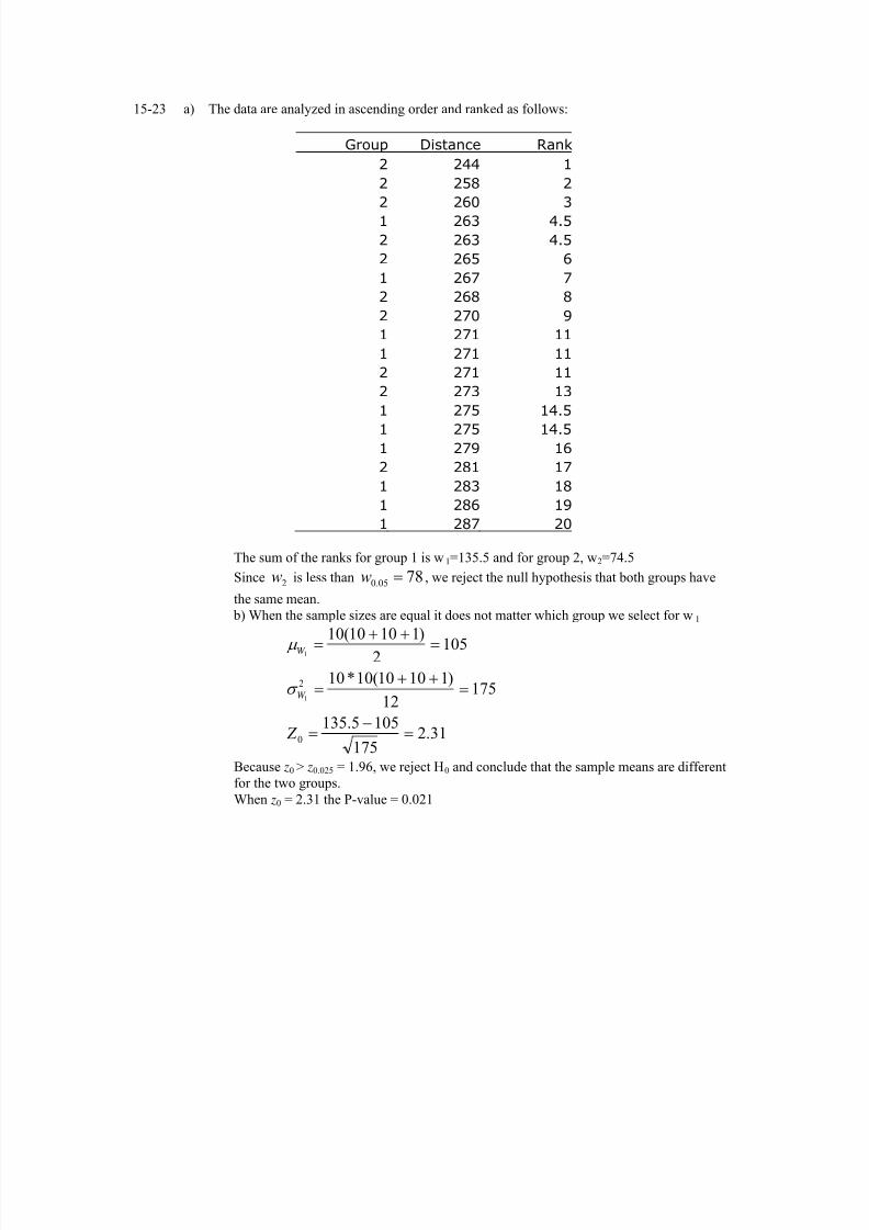
7/12/2019 Solution Manual Stats
http://slidepdf.com/reader/full/solution-manual-stats 510/588
15-23 a) The data are analyzed in ascending order and ranked as follows:
Group Distance Rank
2 244 1
2 258 2
2 260 3
1 263 4.5
2 263 4.5
2 265 6
1 267 7
2 268 8
2 270 9
1 271 11
1 271 11
2 271 11
2 273 13
1 275 14.5
1 275 14.5
1 279 16
2 281 17
1 283 18
1 286 19
1 287 20
The sum of the ranks for group 1 is w1=135.5 and for group 2, w2=74.5
Since is less than2
w0.05 78w = , we reject the null hypothesis that both groups have
the same mean.
b) When the sample sizes are equal it does not matter which group we select for w1
31.2175
1055.135
17512
)11010(10*10
1052
)11010(10
0
2
1
1
=−
=
=++
=
=++=
Z
W
W
σ
μ
Because z0 > z0.025 = 1.96, we reject H0 and conclude that the sample means are different
for the two groups.
When z0 = 2.31 the P-value = 0.021

7/12/2019 Solution Manual Stats
http://slidepdf.com/reader/full/solution-manual-stats 511/588
Section 15-5
15-24 a) Kruskal-Wallis Test on strength
methods N Median Ave Rank Z
1 5 550.0 8.7 0.43
2 5 553.0 10.7 1.65
3 5 528.0 4.6 -2.08
Overall 15 8.0
15-10

7/12/2019 Solution Manual Stats
http://slidepdf.com/reader/full/solution-manual-stats 512/588
H = 4.83 DF = 2 P = 0.089
H = 4.84 DF = 2 P = 0.089 (adjusted for ties)
Do not reject H0. The conditioning method does not have an effect on the breaking strength at α = 0.05.
b) The P-value is about 0.089 (use the chi-square distribution)
15-25 a) Kruskal-Wallis Test on strengthmixingte N Median Ave Rank Z1 4 2945 9.6 0.552 4 3075 12.9 2.123 4 2942 9.0 0.244 4 2650 2.5 -2.91Overall 16 8.5H = 10.00 DF = 3 P = 0.019H = 10.03 DF = 3 P = 0.018 (adjusted for ties)* NOTE * One or more small samples
Reject H0 and conclude that the mixing technique has an effect on the strength.
b) P-value = 0.018 (use the chi-square distribution)
15-26 a) Kruskal-Wallis Test on angle
manufact N Median Ave Rank Z1 5 39.00 7.6 -1.272 5 44.00 12.4 0.833 5 48.00 15.8 2.314 5 30.00 6.2 -1.88Overall 20 10.5H = 8.37 DF = 3 P = 0.039
Do not reject H0. There is not a significant difference between the manufacturers at α = 0.01.
b) The P-value is about 0.039 (use the chi-square distribution)
15-27 a) Following is the data and ranks for the conductivity test.
Type r_i.
Coating Type 1 141 143 146 150
10 12.5 15 19 56.5
Coating Type 2 137 143 149 152
9 12.5 18 20 59.5
Coating Type 3 127 132 133 134
1.5 5.5 7 8 22
Coating Type 4 127 129 129 132
1.5 3.5 3.5 5.5 14
Coating Type 5 142 144 147 148
11 14 16 17 58Since there is a fairly large number of ties, we use Equation 15-12 as the test statistic.
22 1 20(21)
[2868 ]20 1 4
34.89474
s = −−=
and the test statistic is
02.144
)21(20125.2694
89474.34
1 2
=⎥⎦
⎤⎢⎣
⎡−=h
15-11

7/12/2019 Solution Manual Stats
http://slidepdf.com/reader/full/solution-manual-stats 513/588
b) An approximate P-value can be obtained from the approximate chi-squared distribution for H.
Here a = 5 and each n = 4 so that the guidelines for the adequacy of the approximation are not
quite satisfied. The guideline specifies each n > 4.
But if we apply the chi-squared result we use a – 1 = 4 degrees of freedom and determine
0.005 < P-value < 0.01
From Minitab we obtain the following results that agree with the calculated values.
Kruskal-Wallis Test on C1
C2 N Median Ave Rank Z
1 4 144.5 14.1 1.37
2 4 146.0 14.9 1.65
3 4 132.5 5.5 -1.89
4 4 129.0 3.5 -2.65
5 4 145.5 14.5 1.51
Overall 20 10.5
H = 13.98 DF = 4 P = 0.007
H = 14.02 DF = 4 P = 0.007 (adjusted for ties)
Since , we would reject the null hypothesis and conclude that the treatments
differ. Minitab provides the P-value = 0.007
2
0.05,4 9.49h χ > =
15-28 a) Kruskal-Wallis Test on uniformity
flow
rate N Median Ave Rank Z
125 6 3.100 5.8 -2.06
160 6 4.400 13.0 1.97
250 6 3.800 9.7 0.09
Overall 18 9.5
H = 5.42 DF = 2 P = 0.067
H = 5.44 DF = 2 P = 0.066 (adjusted for ties)
Do not reject H0. There is not a significant difference between the flow rates on the uniformity at α = 0.05.
b) P-value = 0.066 (use the chi-square distribution)
15-29 a) D A A D D A A A D D D A
The total number of runs is r = 6.
The observed value of 6 is below the mean of 7. For a sample of size n = 12 with equal samples
from each group, the number of runs can range from 2 to 12. Therefore, the P-value can be
computed as the probability of 6 or fewer or 8 or greater runs. This will be greater usual levels of
significance so that the null hypothesis is not rejected.
The normal approximation can be used for a simpler calculation
6055.0727.2
76
727.2)112(12
)12)6)(6(2(662
)1(
)2(2
712
12)6)(6(22
22
21212
21
−=−
=−
=
=−
−×××=
−
−=
=+
=+
=
R
R
R
R
r z
N N
N nnnn
N
N nn
σ
μ
σ
μ
At α = 0.05 reject H0 when 96.1≥ z . Because 6055.0= z < 1.96, fail to reject H0. There is
not sufficient evidence to conclude that there is a difference in distributions.
15-12

7/12/2019 Solution Manual Stats
http://slidepdf.com/reader/full/solution-manual-stats 514/588
Or, Minitab output:Runs test for C5
Runs above and below K = 1.5
The observed number of runs = 6
The expected number of runs = 7
6 observations above K, 6 below
* N is small, so the following approximation may be invalid.
P-value = 0.545
b) The sum of the ranks for group 1 is w1=40 and for group 2, w2=38
Since both w1 and are both greater than w2w 0.05 =26, there is insufficient evidence to reject the
null hypothesis that both groups have the same mean.
In part (a) we test whether the two samples come from the same distribution. In part (b) we test
whether their means are equal.
15-30
a) The sample numbers of the ranked data are:12112112221121122
The number of runs is r =10.
2665.0955.3
47.910
955.3)117(17
)17)8)(9(2(892
)1(
)2(2
47.917
17)8)(9(22
22
21212
21
=−
=−
=
=−
−×××=
−
−=
=+
=+
=
R
R
R
R
r z
N N
N nnnn
N
N nn
σ
μ
σ
μ
At α = 0.05 reject H0 when . Because96.1|| ≥ z 2665.0= z < 1.96, we fail to reject H0. There is
not enough evidence to conclude that there is a difference in distributions.The P-value ≈ 0.79
Or, using Minitab:Runs test for C5
Runs above and below K = 1.47059
The observed number of runs = 10
The expected number of runs = 9.47059
8 observations above K, 9 below
* N is small, so the following approximation may be invalid.
P-value = 0.790
b)
The sum of the ranks for group 2 (which has the smaller sample size) is 78. Since w0.05=51, wefail to reject H0. There is insufficient evidence to conclude that the groups have the same mean.
Yes, the hypotheses differ. The one from part (a) test whether the samples came from the same
distribution. Here we test whether the populations have the same mean.
15-31
The sample numbers of the ranked data are: 222111112221211112211222; thus, r = 9
15-13
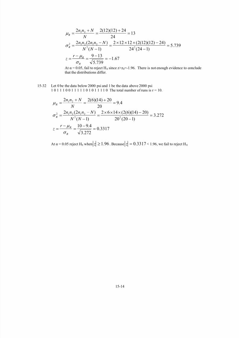
7/12/2019 Solution Manual Stats
http://slidepdf.com/reader/full/solution-manual-stats 515/588
67.1739.5
139
739.5)124(24
)24)12)(12(2(12122
)1(
)2(2
1324
24)12)(12(22
22
21212
21
−=−
=−
=
=−
−×××=
−
−=
=+
=+
=
R
R
R
R
r z
N N
N nnnn
N
N nn
σ
μ
σ
μ
At α = 0.05, fail to reject H0 since z>z0=-1.96. There is not enough evidence to conclude
that the distributions differ.
15-32 Let 0 be the data below 2000 psi and 1 be the data above 2000 psi
1 0 1 1 1 0 0 1 1 1 1 1 0 1 0 1 1 1 1 0 The total number of runs is r = 10.
3317.0272.3
4.910
272.3)120(20
)20)14)(6(2(1462
)1(
)2(2
4.920
20)14)(6(22
22
21212
21
=−
=−
=
=−
−×××
=−
−
=
=+
=+
=
R
R
R
R
r z
N N
N nnnn
N
N nn
σ
μ
σ
μ
At α = 0.05 reject H0 when 96.1≥ z . Because 3317.0= z < 1.96, we fail to reject H0
15-14

7/12/2019 Solution Manual Stats
http://slidepdf.com/reader/full/solution-manual-stats 516/588
Supplemental Exercises
15-33 a)
1. Parameter of interest is median surface finish
0.10~:3
0.10~:.2
1
0
≠
=
μ
μ
H
H
4. α = 0.055. The test statistic is the observed number of plus differences or r + = 5.
6. We reject H 0 if the P-value corresponding to r + = 5 is less than or equal to α = 0.05.
7. Using the binomial distribution with n = 10 and p = 0.5, P-value = 2P( R * ≥ 5| p = 0.5) =1.0
8. Conclusion, we cannot reject H 0. We cannot reject the claim that the median is 10 μin.
b)
1. Parameter of interest is median of surface finish
0.10~:3
0.10~:.2
1
0
≠
=
μ
μ
H
H
4. α=0.05
5. Test statistic is
n
nr z
5.0
5.00
−=
+
6. We reject H 0 if the | Z 0| > Z 0.025 = 1.967. Computation: 0
105.0
)10(5.050 =
−= z
8. Conclusion, cannot reject H 0. There is not sufficient evidence that the median surface finish differs from
10 microinches.
The P-value = 2[1-Φ(0)] = 1
15-34 a)
1. The parameter of interest is the median fluoride emissions.
6~:.3
6~:.2
1
0
<
=
μ
μ
H
H
4. α=0.05
5. The test statistic is the observed number of plus differences or r +
= 4.6. We reject H 0 if the P-value corresponding to r + = 4 is less than or equal to α = 0.05.
7. Using the binomial distribution with n = 15 and p = 0.5, P-value = P(R + ≤ 4 | p = 0.5) = 0.1334
8. Conclusion, do not reject H 0. The data does not support the claim that the median fluoride impurity level
is less than 6.
Using Minitab (Sign Rank Test)Sign test of median = 6.000 versus < 6.000
N Below Equal Above P Mediany 15 9 2 4 0.1334 4.000
Do not reject H0
b)
1. Parameter of interest is median fluoride impurity level
0.6~:3
0.6~:.2
1
0
<
=
μ
μ
H
H
4. α=0.05
5. Test statistic is
n
nr z
5.0
5.00
−=
+
6. We reject H 0 if the Z 0 < -Z 0.05 = -1.65
7. Computation: 39.1135.0
)13(5.040 −=
−= z
15-15

7/12/2019 Solution Manual Stats
http://slidepdf.com/reader/full/solution-manual-stats 517/588
8. Conclusion, do not reject H 0. There is not enough evidence to conclude that the median fluoride impurity
level is less than 6.0 ppm. The P-value = 2[1-Φ(1.39)] = 0.1645.
15-35 1. Parameters of interest are the mean weights
0:.3
0:.2
1
0
≠
=
D
D
H
H
μ
μ
4. α=0.055. The test statistic is w = min( w +, w -).
6. We reject H 0 if w ≤ = 8 because α = 0.05 and n = 10 Appendix A, Table IX gives the critical value.*
05.0w
7. w+
= 55 and w -= 0 and w = min(55, 0) = 0
8. Conclusion, because 0 < 8, we reject H 0 and conclude that there is a difference in the weights due to the
diet modification experiment.
15-36 1. Parameter of interest is the difference between the impurity levels.
0~:.3
0~:.2
1
0
≠
=
D
D
H
H
μ
μ
4. α = 0.05
5. The test statistic r = min(r +, r -).
6. Because α = 0.05 and n = 7, Appendix A, Table VIII gives the critical value of = 0. We reject*05.0r
H 0 in favor of H 1 if r ≤ 10.
7. r + = 1 and r - = 6 and r = min(1,6) = 1
8. Conclusion, cannot reject H 0. There is not a significant difference in the impurity levels.
15-37 a)
1. The parameters of interest are the mean mileages for a Volkswagen and Mercedes.
211
210
:.3
:.2
μ μ
μ μ
≠
=
H
H
4. α = 0.01
5. The test statistic is1
21212
2
)1)((w
nnnnw −
+++=
6. We reject H 0 if w ≤ = 71, because α = 0.01 and n*
01.0w 1 = 10 and n2 = 10, Appendix A, Table X gives the
critical value.
7. w1 = 55 and w2 = 155 and because 55 is less than 71, we reject H 08. Conclusion, reject H0 and conclude that there is a difference in the mean mileages of the two different
vehicles.
b)
1. The parameters of interest are the mean mileages for a Volkswagen and Mercedes
211
210
:.3
:.2
μ μ
μ μ
≠
=
H
H
4. α = 0.01
5. The test statistic is
1
11
0
w
wW
z
σ
μ −=
6. We reject H 0 if | Z 0| > Z 0.005 = 2.58
7. w1 = 55,1w
μ =105 and =1752
1wσ
78.323.13
105550 −=
−= z
Because | Z 0| > 2.58, reject H 08. Conclusion, reject H 0 and conclude that there is a significant difference in the mean mileages at α = 0.01.
P-value =2[1 - P(Z < 3.78 )] = 0.00016
15-16

7/12/2019 Solution Manual Stats
http://slidepdf.com/reader/full/solution-manual-stats 518/588
15-38 a)
1. The parameters of interest are the in mean fill volumes
211
210
:.3
:.2
μ μ
μ μ
≠
=
H
H
4. α=0.05
5. The test statistic1
21212
2
)1)((w
nnnnw −
+++=
6. We reject if H 0 w ≤ = 78, because α = 0.05 and n*
05.0w 1 = 10 and n2 = 10, Appendix A, Table X gives
the critical value.
7. w1 = 58 and w2 = 152 and because 58 is less than 78, we reject H 08. Conclusion, reject H0 and conclude that there is a significant difference in the mean fill volumes at α =
0.05.
b)
1. The parameters of interest are the mean mileages for a Volkswagen and Mercedes
211
210
:.3
:.2
μ μ
μ μ
≠
=
H
H
4. α=0.05
5. The test statistic is
1
11
0
w
wW
z σ
μ −
=
6. We reject H 0 if | Z 0| > Z 0.025 = 1.96
7. w1 = 58,1w
μ = 105 and = 1752
1wσ
55.323.13
105580 −=
−= z
Because | Z 0| > 1.96, reject H 08. Conclusion, reject H 0 and conclude that there is a significant difference in the mean mileages at α = 0.05.
P-value =2[1 - P(Z < 3.55 )] ≅ 0.000385
15-39 Kruskal-Wallis Test on RESISTAN ALLOY N Median Ave Rank Z1 10 98.00 5.7 -4.312 10 102.50 15.3 -0.09
3 10 138.50 25.5 4.40Overall 30 15.5
H = 25.30 DF = 2 P = 0.000H = 25.45 DF = 2 P = 0.000 (adjusted for ties)
Reject H0, P-value ≅ 0
15-40 Kruskal-Wallis Test on TIME
time N Median Ave Rank Z
0 9 1106.0 24.8 2.06
7 9 672.2 19.7 0.38
14 9 646.2 20.9 0.79
21 9 377.6 8.7 -3.23
Overall 36 18.5
H = 11.61 DF = 3 P = 0.009
Reject H0 at α = 0.05
15-41 Kruskal-Wallis Test on VOLUMETEMPERAT N Median Ave Rank Z70 5 1245 12.4 2.6975 5 1220 7.9 -0.0680 5 1170 3.7 -2.63Overall 15 8.0H = 9.46 DF = 2 P = 0.009
15-17

7/12/2019 Solution Manual Stats
http://slidepdf.com/reader/full/solution-manual-stats 519/588
H = 9.57 DF = 2 P = 0.008 (adjusted for ties)
Reject H0 at α = 0.05
15-42 Kruskal-Wallis Test on C4
C5 N Median Ave Rank Z1 10 68.55 13.2 -1.01
2 10 379.20 20.4 2.16
3 10 149.75 12.9 -1.14
Overall 30 15.5
H = 4.65 DF = 2 P = 0.098
Since P=0.098<0.1, we would reject the null hypothesis and conclude that the treatments
differ.
15-18

7/12/2019 Solution Manual Stats
http://slidepdf.com/reader/full/solution-manual-stats 520/588
Mind Expanding Exercises
16-81 a) According to Table 16-10, if there is no shift, ARL=500.
If the shift in mean is 1 X
σ , ARL=17.5.
b) According to Table 16-10, if there is no shift, ARL=500.
If the shift in mean is 2 X
σ , ARL=3.63.
16-82 a) I-MR chart for Refining percentage
Observat ion
I n d i v i d u a l V a l u e
635649423528211471
30
20
10
_
X=15.65
UC L=25.26
LCL=6.04
Observat ion
M
o v i n g
R a n g e
635649423528211471
15
10
5
0
__
MR=3.61
UC L=11.81
LCL=0
1
1
1
11
I -MR Chart of r efine
I-MR chart for Dist& Marketing percentage
Observat ion
I n d i v i d u a l V a l u e
635649423528211471
25
20
15
10
5
_ X=12.45
UC L=23.34
LCL=1.56
Observat ion
M
o v i n g
R a n g e
635649423528211471
16
12
8
4
0
__
MR=4.09
UC L=13.38
LCL=0
1
1
I -MR Chart of distr ibuti on
16-58

7/12/2019 Solution Manual Stats
http://slidepdf.com/reader/full/solution-manual-stats 521/588
b) I-MR chart for crude oil percentage of retail price. It appears there have been a couple of shifts
in the process around observations 16 and 56.
Observat ion
I n d i v i d u a l V a
l u e
635649423528211471
55
50
45
40
35
_
X=44.63
UC L=50.45
LCL=38.82
Observat ion
M
o v i n g
R a n g e
635649423528211471
8
6
4
2
0
__ MR=2.185
UC L=7.139
LCL=0
11
1
11
1
1
1
1
111
1111
1
1
I -MR Chart of cr ude
c)
Observat ion
I n d i v i d u a l V a l u e
635649423528211471
60
40
20
_ X=25.41
UC L=41.85
LCL=8.97
Observat ion
M
o v i n g
R a n g e
635649423528211471
24
18
12
6
0
__ MR=6.18
UC L=20.20
LCL=0
1
1
1
1
1
1
11
I -MR Chart of ref ine_v
16-59

7/12/2019 Solution Manual Stats
http://slidepdf.com/reader/full/solution-manual-stats 522/588
Observat ion
I n d i v i d u a l V a l u e
635649423528211471
40
30
20
10
0
_ X=19.56
UC L=37.02
LCL=2.09
Observat ion
M
o v i n g
R a n g e
635649423528211471
24
18
12
6
0
__ MR=6.57
UC L=21.46
LCL=0
11
1
I -MR Chart of distr ibuti on_v
16-83 Let p denote the probability that a point plots outside of the control limits when the mean has shifted from μ0 to
μ = μ0 + 1.5σ. Then:
( )
( )5.0)06(
4when5.135.13
3/
5.1
/3
/
5.1
5.1|33
5.1|1
000
0
=<<−=
=−+<<−−=
⎟⎟ ⎠
⎞⎜⎜⎝
⎛ +
−<
−<−
−=
⎟⎟ ⎠
⎞⎜⎜⎝
⎛ +=+<<−=
+=<<=−
Z P
nn Z nP
nn
X
nP
n X
nP
UCL X LCLP p
σ
σ
σ
μ
σ
σ
σ μ μ σ
μ σ
μ
σ μ μ
Therefore, the probability the shift is undetected for three consecutive samples is (1 - p)3 = 0.53 =0. 125.
If 2-sigma control limits were used, then
( )
1587.001587.0)15(
4when2/
5.1
/2
/
5.1
5.1|225.1|1 0000
=−=−<<−=
=⎟⎟ ⎠
⎞⎜⎜⎝
⎛ +
−<
−<−
−=
⎟⎟ ⎠
⎞⎜⎜⎝
⎛ +=+<<−=+=<<=−
Z P
nnn
X
nP
n X
nPUCL X LCLP p
σ
σ
σ
μ
σ
σ
σ μ μ σ
μ σ
μ σ μ μ
Therefore, the probability the shift is undetected for three consecutive samples is (1 - p)3 = 0.15873 = 0.004.
16-84
nk UCL
CLnk LCL
/
/
0
0
0
σ μ
μ σ μ
+=
= −=
a)
16-60

7/12/2019 Solution Manual Stats
http://slidepdf.com/reader/full/solution-manual-stats 523/588
( )
]()([1
)(1
///11
|1
|11
000
0
nk nk
nk Z nk P
nk
n
X
nk P
nk X
nk P
UCL X LCLP p
δ δ
δ δ
σ
δσ
σ
μ
σ
δσ
δσ μ μ σ
μ σ
μ
δσ μ μ
−Φ−−Φ−=
−<<−−−=⎟⎟ ⎠
⎞
⎜⎜⎝
⎛ −<
−<−−−=
⎟⎟ ⎠
⎞⎜⎜⎝
⎛ +=+<<−−=
+=<<−=−
where Φ(Z) is the standard normal cumulative distribution function.
16-85
nk UCL
CL
nk LCL
/
/
0
0
0
σ μ
μ
σ μ
+=
=
−=
a) ARL = 1/ p where p is the probability a point plots outside of the control limits. Then,
( )
1)(2)()()(
|/
|1 00
0
−Φ=−Φ−Φ=<<−=
⎟⎟ ⎠
⎞⎜⎜⎝
⎛ <
−<−=<<=−
k k k k Z k P
k n
X k PUCL X LCLP p μ
σ
μ μ
where Φ(Z) is the standard normal cumulative distribution function. Therefore, p = 2 − 2Φ(k) and ARL =
1/[2−2Φ(k)]. The mean time until a false alarm is 1/ p hours.
b) ARL = 1/ p where
( )
( )
)()(1
)()(
//|1 01
δ δ
δ δ
δ δ
σ
δσ
σ
δσ δσ μ μ
nk nk p
and
nk nk
nk Z nk P
nk X
nk PUCL X LCLP p
−−Φ+−Φ−=
−−Φ−−Φ=−<<−−=
⎟ ⎠
⎞⎜⎝
⎛ −<<−−=+=<<=−
c) ARL = 1/ p where 1 - p = P(-3<Z<3)= 0.9973. Thus, ARL = 1/0.0027 = 370.4.
If k = 2, 1 - p = P(-2<Z<2) = 0.9545 and ARL = 1/ p = 22.0.
The 2-sigma limits result in a false alarm for every 22 points on the average. This is a high number of false
alarms for the routine use of a control chart.
d) From part (b), ARL = 1/ p, where 1 - p = P Z( )− − < < − =3 5 3 5 0 7764. . ARL = 4.47 assuming 3-sigma control limits.
16-86 Determine n such that
16-61

7/12/2019 Solution Manual Stats
http://slidepdf.com/reader/full/solution-manual-stats 524/588
⎟⎟⎟⎟
⎠
⎞
⎜⎜⎜⎜
⎝
⎛
−
−−
−
−<<
−
−−
−
−=
⎟⎟⎟⎟
⎠
⎞
⎜⎜⎜⎜
⎝
⎛
=−
−−
+<
−
−<
−
−−
−=
=<<=
)1(
)1(
)1()1(
)1(
)1(
|)1(
)1(
)1()1(
)1(
)|ˆ(5.0
cccc
c
cccc
c
c
cc
c
cc
c
cc
c
c
p p
p pk
n
p p
p p Z
p p
p pk
n
p p
p pP
p p
n
p p
pn
p pk p
n
p p
pP
n
p p
pn
p pk p
P
p pUCLP LCLP
Use the fact that if pc > p then the probability is approximately equal to the probability that Z is less than the
upper limit.
⎟
⎟⎟⎟
⎠
⎞
⎜
⎜⎜⎜
⎝
⎛
−
−−
−
−<≅
)1(
)1(
)1(cccc
c
p p
p pk
n
p p
p p Z P
Then, the probability above approximately equals 0.5 if
)1(
)1(
)1( cccc
c
p p
p pk
n
p p
p p
−
−=
−
−
Solving for n,2
2
)(
)1(
c p p
p pk n
−−
=
16-87 The LCL is
n
p pk p
)1( −−
n
p pk p
)1( −− = 0 or
p
pk n
)1(2 −=
16-88 The P is desired. Now, using the normal approximation:LCL P UCL p( | .< < = 0 08)
90.0)29.1(
100
)08.01(08.0
08.0115.0
100
)08.01(08.0
08.0ˆ
)08.0|115.0ˆ()08.0|115.0ˆ0(
115.0100
)95.0(05.0305.0
)1(3
0015.0100
)95.0(05.0305.0
)1(3
=<=
⎟⎟⎟⎟
⎠
⎞
⎜⎜⎜⎜
⎝
⎛
−
−<
−
−=
=<==<<
=+=−
+=
→−=−=−
−=
Z PP
P
pPP pPP
n
p p pUCL
n
p p p LCL
16-62

7/12/2019 Solution Manual Stats
http://slidepdf.com/reader/full/solution-manual-stats 525/588
Therefore, the probability of detecting shift on the first sample following the shift is 1 − 0.90 = 0.10.
The probability of detecting a shift by at least the third sample following the shift can be determined from the
geometric distribution to be 0.10 + 0.90(0.10) + 0.902(0.10) = 0.27
16-89 The process should be centered at the middle of the specifications; that is, at 100.
For an x chart:
84.0)15(
2/5
1055.107
2/5
105
2/5
1055.92)105|(
5.1072/)5(3100/
5.922/)5(3100/
100
5.1072/)5(3100/
0
0
0
0
=<<−=
⎟⎟ ⎠
⎞⎜⎜⎝
⎛ −<
−<
−==<<
=+=+=
=−=−=
===+=−=
Z P
X PUCL X LCLP
nk UCL
nk LCL
CL
nk UCL
μ
σ μ
σ μ
μ
σ μ
The requested probability is then 1 − 0.84 = 0.16. The ARL = 1/0.16 = 6.25. With μ = 105, the
specifications at 100 ± 15 and σ = 5, the probability of a defective item is
0228.0)2()4(
5105115
5105
510585
5105)115()85(
=>+−<=
⎟ ⎠ ⎞⎜
⎝ ⎛ −>−+⎟
⎠ ⎞⎜
⎝ ⎛ −<−=>+<
Z P Z P
X P X P X P X P
Therefore, the average number of observations until a defective occurs, follows from the geometric
distribution to be 1/0.0228 = 43.86. However, the x chart only requires 6.25 samples of 4 observations each
= 6.25(4) = 25 observations, on average, to detect the shift.
16-90 Let X denote the number of defectives in a sample of n. Then X has a binomial distribution with E( X ) = np
and V( X ) = np(1 - p). Therefore, the estimates of the mean and standard deviation of X are np and
)1( p pn − , respectively. Using these estimates results in the given control limits.
b) Data from example 16-4
20100
55
45
35
25
Sample Number
S a m p l e C o u n t
NP Chart for defectiv
NP=40.00
3.0SL=54.70
-3.0SL=25.30
c) Note that
n
p p pP
n
p p p
p pn pnPn p pn pn
)1(3ˆ)1(
3
)1(3ˆ)1(3
−+<<
−−
−+<<−−
16-63
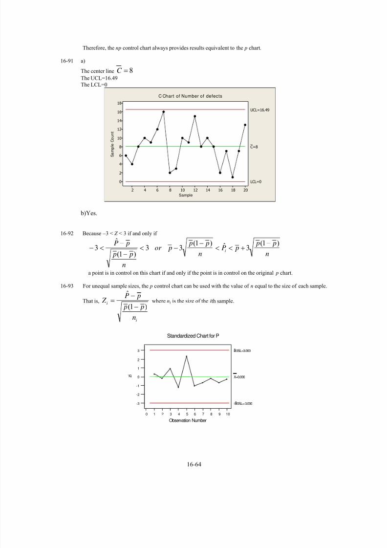
7/12/2019 Solution Manual Stats
http://slidepdf.com/reader/full/solution-manual-stats 526/588
Therefore, the np control chart always provides results equivalent to the p chart.
16-91 a)
The center line 8C =
The UCL=16.49
The LCL=0
Sample
S a m p l e C o u n t
2018161412108642
18
16
14
12
10
8
6
4
2
0
_ C=8
UCL=16.49
LCL=0
C Chart of Number of defects
b)Yes.
16-92 Because −3 < Z < 3 if and only if
n
p p pP
n
p p por
n
p p
pPi
)1(3ˆ)1(
33)1(
ˆ3
−+<<
−−<
−
−<−
a point is in control on this chart if and only if the point is in control on the original p chart.
16-93 For unequal sample sizes, the p control chart can be used with the value of n equal to the size of each sample.
That is,
i
i
n
p p
pP Z
)1(
ˆ
−
−= where ni is the size of the ith sample.
109876543210
3
2
1
0
-1
-2
-3
Observation Number
z i
Standardized Chart for P
X=0.000
3.0SL=3.0003
-3.0SL=-3.000-3
16-64

7/12/2019 Solution Manual Stats
http://slidepdf.com/reader/full/solution-manual-stats 527/588
16-65

7/12/2019 Solution Manual Stats
http://slidepdf.com/reader/full/solution-manual-stats 528/588
CHAPTER 16
Note to the Instructor: Many of the control charts and control chart summaries were created using
Statgraphics. Minitab can be used to provide similar results.
Section 16-5
16-1 a) 286.3435
120022335
7805 ==== r x
0)286.34(0
286.34
51.72)286.34(115.2
22.203)286.34(577.0223
223
78.242)286.34(577.0223
3
4
2
2
===
=
===
=−=−=
=
=+=+=
r D LCL
CL
r DUCL
chart R
r ACL LCL
CL
r ACLUCL
chart x
b)
74.14326.2
286.34ˆ
223ˆ
2
===
==
d
r
x
σ
μ
16-2 a) 1456.025
64.3344.0
25
60.8510.14
25
75.362====== sr x
0)344.0(0
344.0728.0)344.0(115.2
312.14)344.0(577.0510.14
510.14
708.14)344.0(577.0510.14
3
4
2
2
===
====
=−=−=
=
=+=+=
r D LCL
CLr DUCL
chart R
r ACL LCL
CL
r ACLUCL
chart x
16-1

7/12/2019 Solution Manual Stats
http://slidepdf.com/reader/full/solution-manual-stats 529/588
b) c4 = 0.94
00129.094.0194.0
1456.031456.013
1456.0
3041.094.0194.0
1456.031456.013
417.142594.0
1456.03510.143
510.14
603.142594.0
1456.03510.143
224
4
22
4
4
4
4
→−=−⎟ ⎠ ⎞⎜⎝ ⎛ −=−−=
=
=−⎟ ⎠
⎞⎜⎝
⎛ +=−+=
=−=−=
=
=+=+=
cc
ss LCL
CL
cc
ssUCL
chart S
nc
sCL LCL
CL
nc
sCLUCL
chart x
16-3 a) 58.1320
6.271223
20
4460==== s x
061.31512.09213.0
58.13358.1313
58.13
77.301512.09213.0
58.13358.1313
89.200
209213.0
58.1332233
223
11.24549213.0
58.1332233
2
4
4
2
4
4
4
4
→−=⎟ ⎠
⎞⎜⎝
⎛ −=−−=
=
=⎟ ⎠
⎞⎜⎝
⎛ +=−+=
=⎟⎟
⎠
⎞⎜⎜
⎝
⎛ −=−=
=
=⎟⎟ ⎠
⎞⎜⎜⎝
⎛ +=+=
cc
ss LCL
CL
cc
ssUCL
chart S
nc
sCL LCL
CL
nc
sCLUCL
chart x
b) Process mean and standard deviation
74.149213.0
58.13
ˆ223ˆ4 ===== c
s
x σ μ
16-2

7/12/2019 Solution Manual Stats
http://slidepdf.com/reader/full/solution-manual-stats 530/588
16-4 a) 5476.3)534.2(4.1534.24.10.20 2
2
===== r d d
r x
0)5476.3(0
5476.3
11.7)53476.3(004.2
29.18)5476.3(483.00.20
0.20
71.21)5476.3(483.00.20
3
4
2
2
===
=
===
=−=−=
=
=+=+=
r D LCL
CL
r DUCL
chart R
r ACL LCL
CL
r ACLUCL
chart x
043.00946.0)5.1(3427.113
427.1
811.20946.0)5.1(3427.113
427.1so9515.0
16.186/)5.1(30.203
0.20
84.216/)5.1(30.203
5.1/where
2
4
4
2
4
4
4
4
4
4
=−=−−=
=
=+=−+=
==
=−=−=
=
=+=+=
=
cc
sCL LCL
CL
c
c
sCLUCL
scchart S
nc
sCL LCL
CL
nc
sCLUCL
cschart x
16-5 a)X-bar and Range - Initial Study
Problem 16-1
X-bar | Range
----- | -----
UCL: + 3.0 sigma = 37.5789 | UCL: + 3.0 sigma = 11.9461
Centerline = 34.32 | Centerline = 5.65
LCL: - 3.0 sigma = 31.0611 | LCL: - 3.0 sigma = 0
|
out of limits = 1 | out of limits = 0
--------------------------------------------------------------------------------
Chart: Both Normalize: No
20 subgroups, size 5 0 subgroups excluded
Estimated
process mean = 34.32
process sigma = 2.42906
mean Range = 5.65
16-3

7/12/2019 Solution Manual Stats
http://slidepdf.com/reader/full/solution-manual-stats 531/588
0 4 8 12 16 2031
33
35
37
39
34.32
37.5789
31.0611
0 4 8 12 16 2002468
1012
5.65
11.9461
0
Charting xbar
X-bar
Problem 16-5
subgroup
Range
b)
X-bar | Range
----- | -----
UCL: + 3.0 sigma = 37.4038 | UCL: + 3.0 sigma = 12.1297
Centerline = 34.0947 | Centerline = 5.73684
LCL: - 3.0 sigma = 30.7857 | LCL: - 3.0 sigma = 0
|
out of limits = 0 | out of limits = 0
--------------------------------------------------------------------------------
20 subgroups, size 5 1 subgroups excluded
Estimated
process mean = 34.0947
process sigma = 2.4664
mean Range = 5.73684
0 4 8 12 16 2030
32
34
36
38
40
34.0947
37.4038
30.7857
0 4 8 12 16 200
3
6
9
12
15
5.73684
12.1297
0
X-bar
Problem 16-5
subgroup
Range
16-4

7/12/2019 Solution Manual Stats
http://slidepdf.com/reader/full/solution-manual-stats 532/588
16-6 a)X-bar and Range - Initial Study
Charting Problem 16-8
X-bar | Range
----- | -----
UCL: + 3.0 sigma = 7.44253 | UCL: + 3.0 sigma = 2.9153
Centerline = 6.2836 | Centerline = 1.1328
LCL: - 3.0 sigma = 5.12467 | LCL: - 3.0 sigma = 0
|
out of limits = 0 | out of limits = 0
Estimated
process mean = 6.2836
process sigma = 0.669108
mean Range = 1.1328
0 5 10 15 20 25
5.15.55.96.36.77.17.5
6.2836
7.44253
5.12467
0 5 10 15 20 250
0.51
1.52
2.53
1.1328
2.9153
0
X-bar
Problem 16-6
subgroup
Range
There are no points beyond the control limits. The process appears to be in control.
b) No points fell beyond the control limits. The limits do not need to be revised.
16-7 a) X-bar and Range - Initial Study
Charting Problem 16-7
X-bar | Range
----- | -----
UCL: + 3.0 sigma = 17.4 | UCL: + 3.0 sigma = 5.792
Centerline = 15.09 | Centerline = 2.25
LCL: - 3.0 sigma = 12.79 | LCL: - 3.0 sigma = 0
|
Test Results: X-bar One point more than 3.00 sigmas from center line.
Test Failed at points: 4 6 7 10 12 15 16 20
Test Results for R Chart: One point more than 3.00 sigmas from center line.
16-5

7/12/2019 Solution Manual Stats
http://slidepdf.com/reader/full/solution-manual-stats 533/588
Test Failed at points: 19
2010Subgroup 0
20
15
10 S a m p l e
M e a n
1
1
1
1
1
1
11
Mean=15.09
UCL=17.40
LCL=12.79
.
b) Removed points 4, 6, 7, 10, 12, 15, 16, 19, and 20 and revised the control limits. The control limits are not
as wide after being revised: X-bar UCL=17.96, CL=15.78, LCL=13.62 and R UCL = 5.453, R-bar = 2.118,
LCL=0.
c) X-bar and StDev - Initial Study
Charting Problem 16-7
X-bar | StDev
----- | -----
UCL: + 3.0 sigma = 17.42 | UCL: + 3.0 sigma = 3.051
Centerline = 15.09 | Centerline = 1.188LCL: - 3.0 sigma = 12.77 | LCL: - 3.0 sigma = 0
|
Test Results: X-bar One point more than 3.00 sigmas from center line.
Test Failed at points: 4 6 7 10 12 15 16 20
Test Results for S Chart:One point more than 3.00 sigmas from center line.
Test Failed at points: 19
.
6
5
4
3
2
1
0
1
S a m p l e R a n g e
R=2.25
UCL=5.792
LCL=0
Xbar/R Chart for x1-x3
105Subgroup 0
18
17
16
15
14
13
S a m p l e M e a n
Mean=15.78
UCL=17.95
LCL=13.62
6
5
4
3
2
1
0 S a m p l e R a n g e
R=2.118
UCL=5.453
LCL=0
Revised Control Limits
Xbar/R Chart for x1-x3
16-6

7/12/2019 Solution Manual Stats
http://slidepdf.com/reader/full/solution-manual-stats 534/588
0Subgroup 10 20
10
15
20
S a m p
l e M e a n
1
1
1
1
1
1
11
Mean=15.09
UCL=17.42
LCL=12.77
1
Removed points 4, 6, 7, 10, 12, 15, 16, 19, and 20 and revised the control limits. The control limits
are not as wide after being revised: X-bar UCL = 17.95, CL =1 5.78, LCL=13.62 and S UCL =
2.848, S-bar=1.109, LCL=0.
0
1
2
3
S a m p l e S t D e v
S=1.188
UCL=3.051
LCL=0
Xbar/S Chart for x1-x3
105Subgroup 0
18
17
16
15
14
13
S a m p l e M e a n
Mean=15.78
UCL=17.95
LCL=13.62
3
2
1
0 S a m p l e S t D e v
S=1.109
UCL=2.848
LCL=0
Revised Control Limits
Xbar/S Chart for x1-x3
16-7

7/12/2019 Solution Manual Stats
http://slidepdf.com/reader/full/solution-manual-stats 535/588
16-8
a) The average range is used to estimate the standard deviation. Sample 2, 9, and 17 are out-of-control
Sample
S a m
p l e
M
e a n
2018161412108642
4.98
4.97
4.96
4.95
4.94
_ _ X=4.96065
UC L=4.97331
LCL=4.94799
Sample
S a
m
p l e
R a n g e
2018161412108642
0.060
0.045
0.030
0.015
0.000
_ R=0.02195
UC L=0.04641
LCL=0
1
1
1
Xbar-R Chart of x1, ..., x5
b)
Sample
S a
m
p l e
M
e a n
161412108642
4.970
4.965
4.960
4.955
4.950
_ _ X=4.96124
UC L=4.97284
LCL=4.94963
Sample
S a m
p l e
R a n g e
161412108642
0.04
0.03
0.02
0.01
0.00
_ R=0.02012
UC L=0.04254
LCL=0
Xbar-R Chart of x1_ 1, ..., x5_1
16-8

7/12/2019 Solution Manual Stats
http://slidepdf.com/reader/full/solution-manual-stats 536/588
c) For X -S chart
Sample
S a m
p l e
M e a n
2018161412108642
4.98
4.97
4.96
4.95
4.94
_ _ X=4.96065
UC L=4.97333
LCL=4.94797
Sample
S a m
p l e
S t D e v
2018161412108642
0.020
0.015
0.010
0.005
0.000
_ S=0.00888
UC L=0.01855
LCL=0
1
1
1
Xbar-S Chart of x 1, ..., x5
Sample
S a m
p l e
M
e a n
161412108642
4.970
4.965
4.960
4.955
4.950
_ _ X=4.96124
UC L=4.97305
LCL=4.94942
Sample
S a m
p l e
S t D e v
161412108642
0.020
0.015
0.010
0.005
0.000
_ S=0.00828
UC L=0.01730
LCL=0
1
Xbar-S Chart of x1_ 1, ..., x5_ 1
16-9 a)
The control limits for the following chart were obtained from an estimate of σ obtained from the pooled standard deviation from each subgroup of size 5.
16-9
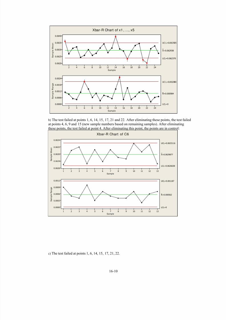
7/12/2019 Solution Manual Stats
http://slidepdf.com/reader/full/solution-manual-stats 537/588
Sample
S a m
p l e
M
e a n
24222018161412108642
0.0640
0.0635
0.0630
0.0625
0.0620
_ _ X=0.062938
UC L=0.063505
LCL=0.062370
Sample
S a m
p l e
R a n g e
24222018161412108642
0.0024
0.0018
0.0012
0.0006
0.0000
_ R=0.000984
UC L=0.002080
LCL=0
1
11
1
1
1
1
Xbar-R Chart of x1 , ..., x5
b) The test failed at points 1, 6, 14, 15, 17, 21 and 22. After eliminating these points, the test failed
at points 4, 6, 9 and 15 (new sample numbers based on remaining samples). After eliminating
these points, the test failed at point 4. After eliminating this point, the points are in control:
Sample
S a m
p l e M e a n
13121110987654321
0.0634
0.0632
0.0630
0.0628
0.0626
_ _ X=0.0629877
UCL=0.0633116
LCL=0.0626638
Sample
S a m
p l e R a n g e
13121110987654321
0.0012
0.0009
0.0006
0.0003
0.0000
_ R=0.000562
UCL=0.001187
LCL=0
Xbar-R Chart of C6
c) The test failed at points 1, 6, 14, 15, 17, 21, 22.
16-10
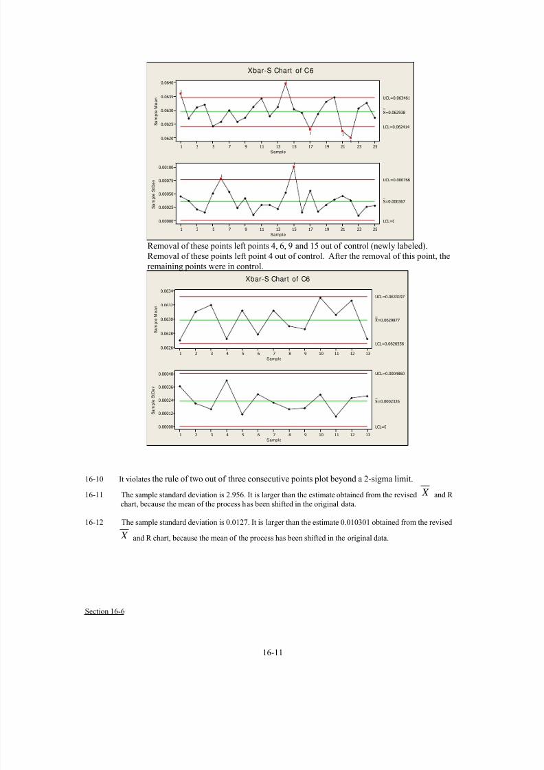
7/12/2019 Solution Manual Stats
http://slidepdf.com/reader/full/solution-manual-stats 538/588
Sample
S a m p l e M e a n
252321191715131197531
0.0640
0.0635
0.0630
0.0625
0.0620
_ _ X=0.062938
UCL=0.063461
LCL=0.062414
Sample
S a m p l e S t D e v
252321191715131197531
0.00100
0.00075
0.00050
0.00025
0.00000
_ S=0.000367
UCL=0.000766
LCL=0
1
11
1
1
1
1
Xbar-S Chart of C6
Removal of these points left points 4, 6, 9 and 15 out of control (newly labeled).
Removal of these points left point 4 out of control. After the removal of this point, the
remaining points were in control.
Sample
S a m
p l e M e a n
13121110987654321
0.0634
0.0632
0.0630
0.0628
0.0626
_ _ X=0.0629877
UCL=0.0633197
LCL=0.0626556
Sample
S a m
p l e S t D e v
13121110987654321
0.00048
0.00036
0.00024
0.00012
0.00000
_ S=0.0002326
UCL=0.0004860
LCL=0
Xbar-S Chart of C6
16-10 It violates the rule of two out of three consecutive points plot beyond a 2-sigma limit.
16-11 The sample standard deviation is 2.956. It is larger than the estimate obtained from the revised X and R
chart, because the mean of the process has been shifted in the original data.
16-12 The sample standard deviation is 0.0127. It is larger than the estimate 0.010301 obtained from the revised
X and R chart, because the mean of the process has been shifted in the original data.
Section 16-6
16-11

7/12/2019 Solution Manual Stats
http://slidepdf.com/reader/full/solution-manual-stats 539/588
Section 16-6
16-11

7/12/2019 Solution Manual Stats
http://slidepdf.com/reader/full/solution-manual-stats 540/588
16-13 a) Individuals and MR(2) - Initial Study
------------------------------------------------------------------------------
Charting Problem 16-13
Ind.x | MR(2)
----- | -----
UCL: + 3.0 sigma = 60.8887 | UCL: + 3.0 sigma = 9.63382
Centerline = 53.05 | Centerline = 2.94737
LCL: - 3.0 sigma = 45.2113 | LCL: - 3.0 sigma = 0
|
out of limits = 0 | out of limits = 0
------------------------------------------------------------------------------
Chart: Both Normalize: No
20 subgroups, size 1 0 subgroups excluded
Estimated
process mean = 53.05
process sigma = 2.61292
mean MR = 2.94737
There are no points beyond the control limits. The process appears to be in control.
0Subgroup 10 20
45
50
55
60
I n d i v i d u a l V a l u e
Mean=53.05
UCL=60.89
LCL=45.21
0
5
10
M o v i n g R a n g e
R=2.947
UCL=9.630
LCL=0
I and MR Chart for hardness
b) Estimated process mean and standard deviation
613.2128.1
94737.2ˆ05.53ˆ2
=====d
mr x σ μ
16-14 a) The process appears to be in statistical control. There are no points beyond the control limits.
16-12
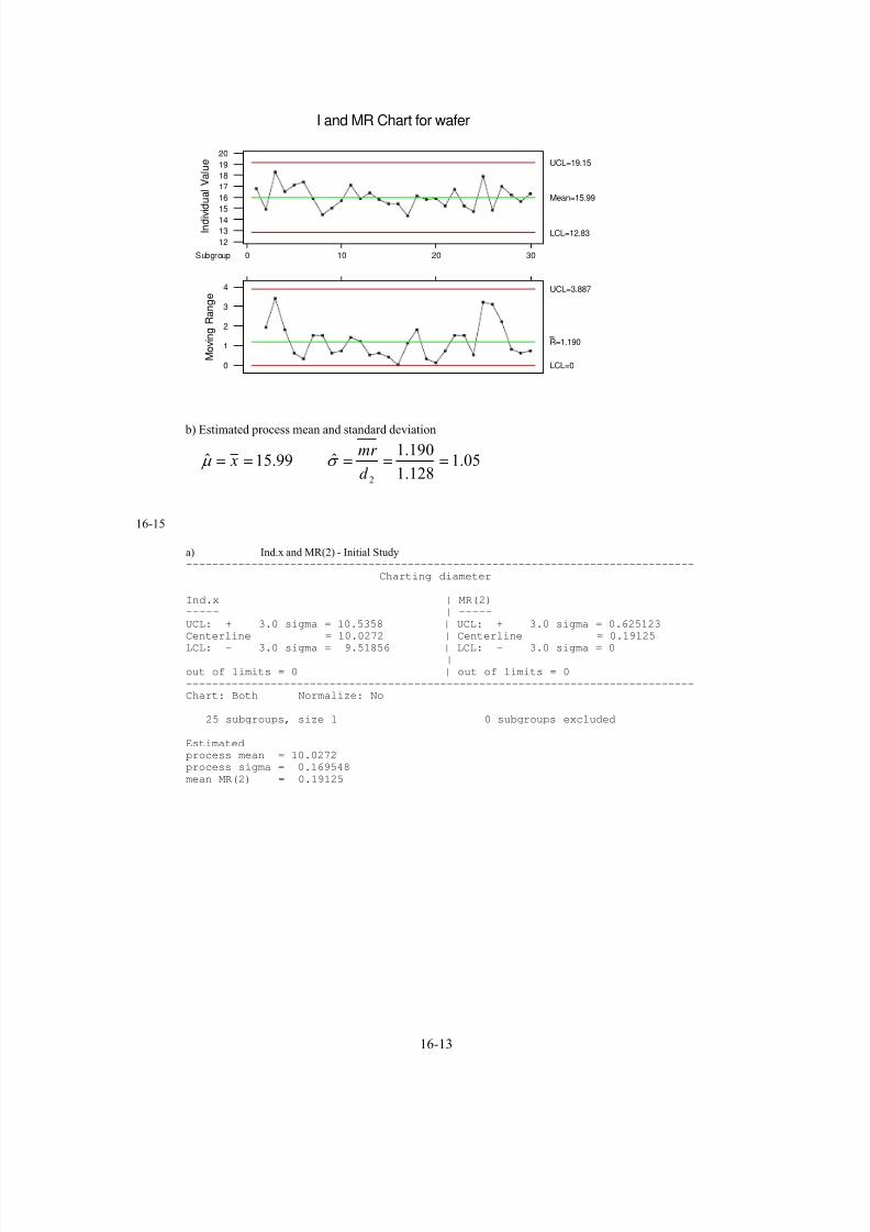
7/12/2019 Solution Manual Stats
http://slidepdf.com/reader/full/solution-manual-stats 541/588
302010Subgroup 0
20
19
18
17
16
1514
13
12
I n d i v i d u a l V a l u e
Mean=15.99
UCL=19.15
LCL=12.83
4
3
2
1
0 M o v i n g R a n g e
R=1.190
UCL=3.887
LCL=0
I and MR Chart for wafer
b) Estimated process mean and standard deviation
05.1128.1
190.1ˆ99.15ˆ
2
=====d
mr x σ μ
16-15
a) Ind.x and MR(2) - Initial Study------------------------------------------------------------------------------
Charting diameter
Ind.x | MR(2)
----- | -----
UCL: + 3.0 sigma = 10.5358 | UCL: + 3.0 sigma = 0.625123
Centerline = 10.0272 | Centerline = 0.19125LCL: - 3.0 sigma = 9.51856 | LCL: - 3.0 sigma = 0
|
out of limits = 0 | out of limits = 0
------------------------------------------------------------------------------
Chart: Both Normalize: No
25 subgroups, size 1 0 subgroups excluded
Estimated
process mean = 10.0272
process sigma = 0.169548
mean MR(2) = 0.19125
16-13

7/12/2019 Solution Manual Stats
http://slidepdf.com/reader/full/solution-manual-stats 542/588
0Subgroup 5 10 15 20 25
9.5
10.0
10.5
I n d i v i d u a l V a l u e
Mean=10.03
UCL=10.54
LCL=9.519
0.0
0.1
0.2
0.3
0.4
0.5
0.6
0.7
M o v i n g R a n g e
R=0.1912
UCL=0.6249
LCL=0
I and MR Chart for Dia
There are no points beyond the control limits. The process appears to be in control.
b) Estimated process mean and standard deviation
16955.0128.1
19125.0ˆ0272.10ˆ
2
=====d
mr x σ μ
16-16 a) Ind.x and MR(2) - Initial Study
--------------------------------------------------------------------------------Charting Problem 16-16
Ind.x | MR(2)
----- | -----
UCL: + 3.0 sigma = 552.112 | UCL: + 3.0 sigma = 63.308
Centerline = 500.6 | Centerline = 19.3684
LCL: - 3.0 sigma = 449.088 | LCL: - 3.0 sigma = 0
|
out of limits = 0 | out of limits = 0
--------------------------------------------------------------------------------
Chart: Both Normalize: No
20 subgroups, size 1 0 subgroups excluded
Estimated
process mean = 500.6
process sigma = 17.1706
mean MR(2) = 19.3684
16-14

7/12/2019 Solution Manual Stats
http://slidepdf.com/reader/full/solution-manual-stats 543/588
0Subgroup 10 20
450
500
550
I n d i v i d u a l V a l u e
Mean=500.6
UCL=552.1
LCL=449.1
0
10
20
30
40
50
60
70
M o v i n g R a n g e
R=19.37
UCL=63.28
LCL=0
I and MR Chart for viscosity
b) Estimated process mean and standard deviation
17.17128.1
3684.19ˆ6.500ˆ
2
=====d
mr x σ μ
16-17
a)
Observat ion
I n d i v i d u a
l V a l u e
24222018161412108642
140
120
100
80
_ X=100.78
UC L=130.50
LCL=71.06
Observat ion
M
o v i n g
R a n g e
24222018161412108642
40
30
20
10
0
__ MR=11.18
UC L=36.51
LCL=0
1
I -MR Chart of SI ZE
Remove the out-of-control observation:
16-15

7/12/2019 Solution Manual Stats
http://slidepdf.com/reader/full/solution-manual-stats 544/588
Observa t ion
I n d i v i d u a l V a l u e
24222018161412108642
120
100
80
_ X=99.48
UC L=127.08
LCL=71.88
Observa t ion
M
o v i n g
R a n g e
24222018161412108642
30
20
10
0
__ MR=10.38
UC L=33.91
LCL=0
I -MR Chart of SI ZE
b) The estimated mean is 99.4792 and estimated standard deviation is 9.20059.

7/12/2019 Solution Manual Stats
http://slidepdf.com/reader/full/solution-manual-stats 545/588
Section 16-7
16-18. a)
The natural tolerance limits are100 18± .
401.1111
6 36
USL LSLPCR
σ
−= = =
Since the mean of the process is centered at the nominal dimension,
1.1111k
PCR PCR= =Since the process natural tolerance limits lie inside the specifications, very few defective units will be
produced.
The fraction defective is 2 ( 20 /6) 0.0858%Φ − =
b)
The natural tolerance limits are106 18± .
401.1111
6 36
USL LSLPCR
σ
−= = =
Since the mean of the process is not centered at the nominal dimension,
14 26min , 0.7778
18 18k
PCR⎡ ⎤= =⎢ ⎥⎣ ⎦
The small PCRK indicates that the process is likely to produce units outside the specification limits.
The fraction defective is
( ) ( )( ) ( ) 14 / 6 26 / 6 0.0098+0=0.0098P X LSL P X USL P Z P Z < + > = < − + > =
16-19 a)12
1.56 6
USL LSLPCR
σ σ
−= = = so 1.3333σ =
b) (20+32)/2=26 When the process is centered at the nominal dimension, the fraction defective is minimized
for any σ .
16-16

7/12/2019 Solution Manual Stats
http://slidepdf.com/reader/full/solution-manual-stats 546/588
16-20 a) The natural tolerance limits are 20 6± .
201.6667
6 12
USL LSLPCR
σ
−= = =
Since the mean of the process is centered at the nominal dimension,
1.6667k
PCR PCR= =
Since the process natural tolerance limits lie inside the specifications, very few defective units will be produced.
The fraction defective is 2 ( 10 / 2) 0Φ − =
b) The natural tolerance limits is 23 6± .
201.6667
6 12
USL LSLPCR
σ
−= = =
Since the mean of the process is not centered at the nominal dimension,
13 7min , 1.1667
6 6k
PCR⎡ ⎤= =⎢ ⎥⎣ ⎦
The fraction defective is
00023.000023.00)2/7()2/13()()( =+=>+−<=>+< Z P Z PUSL X P LSL X P
c) The measure of actual capability decreases and the fraction defective increases when the
process mean is shifted from the center of the specification limits.
16-21 a) If the process uses 66.7% of the specification band, then 6σ = 0.667(USL-LSL). Because the process is
centered
LSU USL
USL LSLUSL
−=−=
−=−=−=
μ μ σ
μ μ μ σ
5.4
)(667.0)(677.0)(667.03
5.13
5.4
,3
5.4
min =⎥⎦
⎤
⎢⎣
⎡
== σ
σ
σ
σ
K PCRPC
Because PCR and PCR k exceed unity, the natural tolerance limits are inside the specification limits and few
defective units should be produced.
b) Assuming a normal distribution with 6σ = 0.667(USL − LSL) and a centered process, then
3σ = 0.667(USL − μ). Consequently, USL − μ = 4.5σ and μ − LSL = 4.5σ
011
)5.4(1)5.4(5.4
)(
=−=
<−=>=⎟ ⎠
⎞⎜⎝
⎛ >=> Z P Z P Z PUSL X Pσ
σ
By symmetry, the fraction defective is 2[P(X > USL)] = 0.
16-22 a) If the process uses 85% of the spec band then 6σ = 0.85(USL − LSL) and
18.185.0
1
)(85.0==
−−
= LSLUSL
LSLUSLPCR
Then 3σ = 0.85(USL − μ) = 0.85(μ − LSL)
Therefore,
18.13
53.3,
3
53.3min =⎥⎦
⎤⎢⎣
⎡=σ
σ
σ
σ
k PCR
16-17

7/12/2019 Solution Manual Stats
http://slidepdf.com/reader/full/solution-manual-stats 547/588
Because PCR and PCR k exceed unity, the natural tolerance limits are inside the specification limits and few
defective units should be produced.
b) Assuming a normal distribution with 6σ = 0.85(USL − LSL) and a centered process, then
3σ = 0.85(USL − μ). Consequently, USL − μ = 3.5σ and μ − LSL = 3.5σ
000233.0999767.01
)5.3(1)5.3(5.3
)(
=−=
<−=>=⎟ ⎠
⎞⎜⎝
⎛ >=> Z P Z P Z PUSL X P
σ
σ
By symmetry, the fraction defective is 2[P(X > USL)] = 0.00046
16-23 Assume a normal distribution with = 223 and =μ σ =326.2
286.3414.74
( ) ( )
00604.099396.01)51.2(1
)51.2(74.14
223260
ˆ
ˆ
)(
00175.0
92.274.14
223180
ˆ
ˆ
=−=<−=>=⎟ ⎠
⎞
⎜⎝
⎛ −
>=⎟ ⎠
⎞
⎜⎝
⎛ −
>=>
=
−<=⎟ ⎠
⎞⎜⎝
⎛ −<=⎟
⎠
⎞⎜⎝
⎛ −<=<
Z P
Z P Z PUSL
Z PUSL X P
Z P Z P LSL
Z P LSL X P
σ
μ
σ
μ
Therefore, the proportion nonconforming is given by
P(X<LSL) + P(X>USL) = 0.00175 + 0.00604 = 0.00779
[ ]837.0
972.0,837.0min
)74.14(3
180223,)74.14(3
223260min
ˆ3,
ˆ3min
905.0)74.14(6
180260
)ˆ(6
=
=
⎥⎦
⎤⎢⎣
⎡ −−=
⎥⎦
⎤⎢⎣
⎡ −−=
=−
=−
=
σ σ
σ
LSL x xUSLPCR
LSLUSLPCR
K
The process capability is marginal.
16-24. a) Assume a normal distribution with = 14.510 andμ .
..σ = = =
r
d2
0 344
23260148
( ) ( )
00028.0
45.3148.0
51.1400.14
ˆ
ˆ
=
−<=⎟ ⎠
⎞⎜⎝
⎛ −<=⎟
⎠
⎞⎜⎝
⎛ −<=< Z P Z P
LSL Z P LSL X P
σ
μ
00047.099953.01)31.3(1
)31.3(148.0
51.1400.15
ˆ
ˆ)(
=−=<−=
>=⎟ ⎠
⎞⎜⎝
⎛ −>=⎟
⎠
⎞⎜⎝
⎛ −>=>
Z P
Z P Z PUSL
Z PUSL X Pσ
μ
Therefore, the proportion nonconforming is given by
P(X<LSL) + P(X>USL) =0.00028 + 0.00047 = 0.00075
16-18

7/12/2019 Solution Manual Stats
http://slidepdf.com/reader/full/solution-manual-stats 548/588
b)
[ ]104.1
15.1,104.1min
)148.0(3
00.1451.14,
)148.0(3
51.1400.15min
ˆ3,
ˆ3min
13.1)148.0(6
00.1400.15
)ˆ(6
=
=
⎥⎦
⎤⎢⎣
⎡ −−=
⎥⎦
⎤⎢⎣
⎡ −−=
=−
=−
=
σ σ
σ
LSL x xUSLPCR
LSLUSLPCR
K
Because PCR and PCR k exceed unity, the natural tolerance limits are inside the specification limits and few
defective units should be produced.
Because PCR K ≅ PCR the process appears to be centered.
16-25 a) Assume a normal distribution with = 223 andμ 74.14
9213.0
58.13ˆ
4
===c
sσ
( ) ( )
00016.0
60.374.14
223170
ˆ
ˆ
=
−<=⎟ ⎠
⎞⎜⎝
⎛ −<=⎟
⎠
⎞⎜⎝
⎛ −<=< Z P Z P
LSL Z P LSL X P
σ
μ
00074.099926.01)18.3(1
)18.3(75.14
223270
ˆ
ˆ)(
=−=<−=
>=⎟ ⎠
⎞⎜⎝
⎛ −>=⎟
⎠
⎞⎜⎝
⎛ −>=>
Z P
Z P Z PUSL
Z PUSL X Pσ
μ
Probability of producing a part outside the specification limits is 0.00016 + 0.00074 = 0.0009
[ ]06.1
19.1,06.1min
)75.14(3
170223,
)75.14(3
223270min
ˆ3,
ˆ3min
13.1)74.14(6
170270
)ˆ(6
=
=
⎥⎦
⎤⎢⎣
⎡ −−=
⎥⎦
⎤⎢⎣
⎡ −−=
=−
=−
=
σ σ
σ
LSL x xUSLPCR
LSLUSL
PCR
K
Because PCR and PCR k exceed unity, the natural tolerance limits are inside the specification limits and few
defective units should be produced. The estimated proportion nonconforming is given by P(X < LSL) + P(X> USL) = 0.00016 + 0.00074 = 0.0009
16-19

7/12/2019 Solution Manual Stats
http://slidepdf.com/reader/full/solution-manual-stats 549/588
16-26 Assuming a normal distribution with = 20.0 and = 1.4μ σ
[ ]19.1
19.1,19.1min
)4.1(3
1520,
)4.1(3
2025min
ˆ3
ˆ,
ˆ3
ˆmin
19.1)4.1(6
1525
)ˆ(6
=
=
⎥⎦
⎤⎢⎣
⎡ −−=
⎥
⎦
⎤⎢
⎣
⎡ −−=
=−
=−
=
σ
μ
σ
μ
σ
LSLUSLPCR
LSLUSLPCR
K
The process is capable.
16-27 a) 446.2326.2
737.5ˆ
2
===d
r σ 0002466.0ˆ =σ
[ ]217.1
217.1,489.1min
)0002466.0(3
5025.05034.0,
)0002466.0(3
5034.05045.0min
ˆ3,
ˆ3min
35.1)0002466.0(6
5025.05045.0)ˆ(6
=
=
⎥⎦
⎤⎢⎣
⎡ −−=
⎥⎦
⎤⎢⎣
⎡ −−=
=−=−=
σ σ
σ
LSL x xUSLPCR
LSLUSLPCR
K
Because PCR and PCR k exceed unity, the natural tolerance limits are inside the specification limits and fewdefective units should be produced.
Because PCR K ≠PCR the process is slightly off center.
b) Assume a normal distribution with = 0.5034 and = 0.0002466μ σ
( ) ( )
011
)46.4(1)46.4(ˆ
ˆ)(
00013.065.3ˆ
ˆ
=−=
<−=>=⎟ ⎠
⎞⎜⎝
⎛ −>=>
=−<=⎟ ⎠
⎞⎜⎝
⎛ −<=<
Z P Z PUSL
Z PUSL X P
Z P LSL
Z P LSL X P
σ
μ
σ
μ
Therefore, the proportion nonconforming is given by
P(X<LSL) + P(X>USL) = 0.00013 + 0 = 0.00013
16-20

7/12/2019 Solution Manual Stats
http://slidepdf.com/reader/full/solution-manual-stats 550/588
16-28 Assuming a normal distribution with = 6.284 and =μ σ693.1
1328.1= 0.669
[ ]357.0
640.0,357.0min
)669.0(3
5284.6,
)669.0(3
284.67min
ˆ3,
ˆ3min
50.0)669.0(6
57
)ˆ(6
=
=
⎥⎦
⎤⎢⎣
⎡ −−=
⎥⎦⎤⎢
⎣⎡ −−=
=−
=−
=
σ σ
σ
LSL x xUSLPCR
LSLUSLPCR
K
The process capability is poor.
16-29 329.1693.1
25.2ˆ
2
===d
r σ
09.15= x
5120.00.05120.0
)96.5()053.0(
693.1
09.155
693.1
09.1515
)5()15(
=+=
−<+−>=
⎟ ⎠
⎞⎜⎝
⎛ −<+⎟
⎠
⎞⎜⎝
⎛ −>=
<+>
Z P Z P
Z P Z P
X P X P
985.0)693.1(6
515 =−=PCR
Because the estimated PCR is less than unity, the process capability is not good.
16-30 Assuming a normal distribution with = 500.6 and = 17.17μ σ
[ ]474.0
50.0,474.0min
)17.17(34756.500,
)17.17(36.500525min
ˆ3,
ˆ3min
49.0)17.17(6
475525
)ˆ(6
=
=
⎥⎦⎤⎢
⎣⎡ −−=
⎥⎦
⎤⎢⎣
⎡ −−=
=−
=−
=
σ σ
σ
LSL x xUSLPCR
LSLUSLPCR
K
Because the process capability ratios are less than unity, the process capability appears to be poor.
16-21

7/12/2019 Solution Manual Stats
http://slidepdf.com/reader/full/solution-manual-stats 551/588
Section 16-8
16-31 a) This process is out of control statistically
Sample
P r o p o r t i o n
2018161412108642
0.14
0.12
0.10
0.08
0.06
0.04
0.02
_ P=0.0645
UCL=0.0835
LCL=0.0455
1
1111
111
1
1
1
1
1
1
1
1
P Char t of C1
b)
Sample
P r o p o r t i o n
2018161412108642
0.14
0.12
0.10
0.08
0.06
0.04
0.02
0.00
_ P=0.0645
UCL=0.1382
LCL=0
11
P Chart of C1
The process is still out of control, but not as many points fall outside of the control limits. The
control limits are wider for smaller values of n.Test Failed at points: 5 and 7.
16-22

7/12/2019 Solution Manual Stats
http://slidepdf.com/reader/full/solution-manual-stats 552/588
The following charts eliminates points 5 and 7.
Sample
P r o p o r t i o n
18161412108642
0.14
0.12
0.10
0.08
0.06
0.04
0.02
0.00
_ P=0.0561
UCL=0.1252
LCL=0
P Chart of C2
c) The larger sample size leads to smaller standard deviation of proportions and thus narrower
control limits.
16-32 a)
0 1 0 2 0 3 0
0 .0
0 .1
0 .2
S a m p l e N u m b e r
P r o p o r t i o n
P C har t f o r x
P = 0 . 0 9 9 3 3
U C L = 0 . 1 8 9 1
L C L = 0 . 0 0 9 6 0 1
b) The process appears to be in statistical control.
16-33P Chart - Initial Study
Charting Problem 16-33
P Chart
-----
UCL: + 3.0 sigma = 0.198553
Centerline = 0.150571
LCL: - 3.0 sigma = 0.10259
out of limits = 12
Estimated
mean P = 0.150571
16-23

7/12/2019 Solution Manual Stats
http://slidepdf.com/reader/full/solution-manual-stats 553/588
sigma = 0.0159937
0 4 8 12 1 6 2 0 2 4
0
0.1
0.2
0.3
0.4
0.150571
0.198553
0.10259
subgroup
P
Problem 16-28
The samples with out-of-control points are 1, 2, 3, 6, 7, 8, 11, 12, 13, 15, 17, and 20. The control limits need
to be revised.
P Chart - Revised Limits
Charting Problem 16-33
P Chart
-----
UCL: + 3.0 sigma = 0.206184
Centerline = 0.157333
LCL: - 3.0 sigma = 0.108482
out of limits = 0
Estimated
mean P = 0.157333
sigma = 0.0162837
0 4 8 12 16 20 24
0
0.1
0.2
0.3
0.4
0.157333
0.206184
0.108482
subgroup
P
Problem 16-28Revised Limits
There are no further points out of control for the revised limits.
16-34 The process does not appear to be in control.
35302520151050
0.02
0.01
0.00
Sample Number
S a m p l e C o u n t
U Chart for defects per 1000 ft
1
1
1
1
U=0.008143
UCL=0.01670
LCL=0
16-24

7/12/2019 Solution Manual Stats
http://slidepdf.com/reader/full/solution-manual-stats 554/588
16-35 a)
2520151050
5
4
3
2
1
0
Sample Number
S a m p l e C o u n t
U Chart for defects
1
1
U=1.942
3.0SL=3.811
-3.0SL=0.07217
Samples 5 and 24 are points beyond the control limits. The limits need to be revised.
b)
0 10 20
0
1
2
3
4
Sample Number
S a m p l e C o u n t
U Chart for defects_
U=1.709
UCL=3.463
LCL=0
The control limits are calculated without the out-of-control points. There are no further points out of control
for the revised limits.
16-36 a)
16-25

7/12/2019 Solution Manual Stats
http://slidepdf.com/reader/full/solution-manual-stats 555/588
Sample
S a m p l e C o u n t P e r U
n i t
1009080706050403020101
45
40
35
30
25
20
15
10
5
_ U=19.51
UCL=32.77
LCL=6.261
1
1
11
1
1
U Chart of Number of Eart hquakes
b) No. The process is out-of-control.

7/12/2019 Solution Manual Stats
http://slidepdf.com/reader/full/solution-manual-stats 556/588
Section 16-9
16-37 a) (112-100)/3=4
b)
( )88 96 112 96
(88 112) 2 44 4
( 4) ( 2) 0.9772
X
X P X P P Z
P Z P Z
μ
σ
⎛ ⎞− − −< < = < < = − < <⎜ ⎟
⎝ ⎠= < − < − =
The probability of detecting is 1-0.9772=0.0228.
c) 1/0.0228=43.8596 ARL to detect the shift is about 44.
16-38 a) UCLn =+
σ μ 3
4)100106(3
2
1064
3100
=−=
=+
σ
σ
b) 96,22
4ˆˆ ==== μ
σ σ
n x
( )
8413.01587.01)1()5(
512
961062
9694)10694(
=−=−<−<=
<<−=⎟⎟ ⎠ ⎞⎜⎜
⎝ ⎛ −<−<−=<<
Z P Z P
Z P X P X P xσ
μ
The probability that this shift will be detected on the next sample is p = 1−0.8413 = 0.1587.
c) 301.61587.0
11===
p ARL
16-26

7/12/2019 Solution Manual Stats
http://slidepdf.com/reader/full/solution-manual-stats 557/588
16-39 a) x = 7401. σx= 0.0045 μ = 74.01
7823.0)11(7823.0)]22.5(1[)78.0(
)22.5()78.0()78.022.5(
0045.0
01.740135.74
ˆ0045.0
01.749865.73
)0135.749865.73(
=−−=<−−<=
−<−<=<<−=
⎟⎟ ⎠
⎞⎜⎜⎝
⎛ −<
−<
−=
<<
Z P Z P
Z P Z P Z P
X P
X P
xσ
μ
The probability that this shift will be detected on the next sample is p = 1−0.7823 = 0.2177.
b) 6.42177.0
11===
p ARL
16-40 a) 148.0326.2
344.0ˆ
2
===d
Rσ σx
= 066.05
148.0ˆ==
n
σ , μ = 14.6
94950.0)0(94950.0
)36.4()64.1()64.136.4(
066.0
6.14708.14
066.0
6.14312.14)708.14312.14(
=−=
−<−<=<<−=
⎟⎟
⎠
⎞⎜⎜
⎝
⎛ −<
−<
−=<<
Z P Z P Z P
X P X P
x
σ
μ
The probability that this shift will be detected on the next sample is p = 1−0.94950 = 0.0505.
b) 8.190505.0
11===
p ARL
16-41 a) 74.14ˆ2
==d
Rσ σx
= .
.σ
n= =
1474
56592 , μ = 210
8485.01515.01
)03.1()97.4()97.403.1(
592.6
21078.242
592.6
21022.203)78.24222.203(
=−=
−<−<=<<−=
⎟⎟
⎠
⎞⎜⎜
⎝
⎛ −<
−<
−=<<
Z P Z P Z P
X P X P
x
σ
μ
The probability that this shift will be detected on the next sample is p = 1−.8485= 0.1515.
b) 6.61515.0
11===
p ARL
16-42 a) 4.1ˆ2
==d
Rσ σx
= 5715.06
4.1ˆ==
n
σ , μ = 17
0119.09881.01
)26.2()24.8()24.826.2(
5715.0
1771.21
5715.0
1729.18)71.2129.18(
=−=
<−<=<<=⎟
⎟
⎠
⎞
⎜
⎜
⎝
⎛ −<
−<
−=<<
Z P Z P Z P
X P X P
xσ
μ
The probability that this shift will be detected on the next sample is p = 1−0.0119 = 0.9881.
b) 012.19881.0
11===
p ARL
16-27

7/12/2019 Solution Manual Stats
http://slidepdf.com/reader/full/solution-manual-stats 558/588
16-43 a) σx= 103.1
5
4664.2ˆ==
n
σ , μ = 36
8980.008980.0 )73.4()27.1()27.173.4(
103.1
36404.37
ˆ103.1
3678.30)404.3778.30(
=−=−<−<=<<−=
⎟⎟ ⎠
⎞⎜⎜⎝
⎛ −<
−<
−=<<
Z P Z P Z P
X P X P
xσ
μ
The probability that this shift will be detected on the next sample is p = 1−0.8980 = 0.1020.
b) 8.9102.0
11===
p ARL
16-44 a) 329.1693.1
25.2ˆ
2
===d
Rσ σx
= 767.03
329.1ˆ==
n
σ , μ = 13
6064.03936.01
)27.0()74.5()74.527.0(
767.0
134.17
767.0
1379.12)4.1779.12(
=−=
−<−<=<<−=
⎟⎟ ⎠
⎞⎜⎜⎝
⎛ −<
−<
−=<<
Z P Z P Z P
X P X P
xσ
μ
The probability that this shift will be detected on the next sample is p = 1−06064 = 0.3936.
b) 54.23936.0
11===
p ARL
16-45 a) 000397.0
326.2
000924.0ˆ
2
===d
Rσ σx
= 000178.0
5
000397.0ˆ==
n
σ , μ = 0.0625
7123.02877.01
)56.0()62.5()62.556.0(
000178.0
0625.00635.0
000178.0
0625.00624.0)0635.00624.0(
=−=
−<−<=<<−=
⎟⎟ ⎠
⎞⎜⎜⎝
⎛ −<
−<
−=<<
Z P Z P Z P
X P X P
xσ
μ
The probability that this shift will be detected on the next sample is p = 1 − 0.7123 = 0.2877.
b) 48.32877.0
11===
p ARL
16-46 a) 669.0ˆ2
==d
Rσ σx
= 386.0
3
669.0ˆ==
n
σ , μ = 5.5
83397.016603.01
)97.0()03.5()03.597.0(
386.0
5.5443.7
0386
5.5125.5)5.5|443.7125.5(
=−=
−<−<=<<−=
⎟⎟ ⎠
⎞⎜⎜⎝
⎛ −<
−<
−==<<
Z P Z P Z P
X P X P
xσ
μ μ
The probability that this shift will be detected on the next sample is p = 1−0.83397 = 0.16603.
16-28

7/12/2019 Solution Manual Stats
http://slidepdf.com/reader/full/solution-manual-stats 559/588
b) 02.616603.0
11===
p ARL

7/12/2019 Solution Manual Stats
http://slidepdf.com/reader/full/solution-manual-stats 560/588
Section 16-10
16-47
a) Yes, this process is in-control. CUSUM chart with h = 4 and k = 0.5 is shown.
Sample
C u m u l a t i v e S u m
151413121110987654321
4
3
2
1
0
-1
-2
-3
-4
0
UCL=3.875
LCL=-3.875
CUSUM Chart of v iscosit y
b) Yes, this process has shifted out-of-control. For the CUSUM estimated from all the data
observation 20 exceeds the upper limit.
16-29

7/12/2019 Solution Manual Stats
http://slidepdf.com/reader/full/solution-manual-stats 561/588
Sample
C u m u l a t i v e S u m
2018161412108642
7.5
5.0
2.5
0.0
-2.5
-5.0
0
UCL=3.88
LCL=-3.88
CUSUM Char t of v iscosi ty
For a CUSUM with standard deviation estimated from the moving range of the first 15 observation, the
moving range is 1.026 and the standard deviation estimate is 0.9096. If this standard deviation is used with a
target of 14.1, the following CUSUM is obtained.
Sample
C u m u l a t i v e
S u m
191715131197531
7.5
5.0
2.5
0.0
-2.5
-5.0
0
UCL=3.64
LCL=-3.64
CUSUM Char t of C1
16-48 a) CUSUM Control chart with k = 0.5 and h = 4
16-30

7/12/2019 Solution Manual Stats
http://slidepdf.com/reader/full/solution-manual-stats 562/588
3
2
1
0
-1
-2
-3
3.2
-3.2
20100
Subgroup Number
C u m u l a t i v e S u m
Upper CUSUM
Lower CUSUM
CUSU M C hart for Purity
The CUSUM control chart for purity does not indicate an out-of-control situation. The SH values do not plot
beyond the values of − H and H .
b) CUSUM Control chart with k = 0.5 and h = 4
3
2
1
0
-1
-2
-3
3.2
-3.2
2520151050
Subgroup Number
C u m u l a t i v e S u m
Upper CUSUM
Lower CUSUM
CUSUM Chart for New Purity Data
The process appears to be moving out of statistical control.
16-49a) σ ˆ = 0.1736
b) CUSUM Control chart with k = 0.5 and h = 4
16-31

7/12/2019 Solution Manual Stats
http://slidepdf.com/reader/full/solution-manual-stats 563/588
-0.5
0.0
0.5
-6.8E-01
0.678191
0 5 10 15 20 25
Subgroup Number
C u m u l a t i v e S u m
Upper CUSUM
Lower CUSUM
CUSUM Chart for Diameter
The process appears to be out of control at the specified target level.
16-50 a) CUSUM Control chart with k = 0.5 and h = 4
-30
-20
-10
0
10
20
30
-32
32
0 10 20
Subgroup Number
C u m u l a t i v e S u m
Upper CUSUM
Lower CUSUM
CUSUM Chart for Concentration
The process appears to be in statistical control.
b) With the target = 100 a shift to 104 is a shift of 104 – 100 = 4 = 0.5σ. From Table 16-9 with h = 4 and a
shift of 0.5, ARL = 26.6
16-51 a) A shift to 51 is a shift of μ μ
σ
−=
−0 51 50
2= 0.5 standard deviations. From Table 16-9, ARL = 38.0
b) If n = 4, the shift to 51 is a shift of
μ μ
σ
−
=
−0 51 50
2 4 / / n = 1 standard deviation. From Table 16-9, ARL =
10.4
16-32

7/12/2019 Solution Manual Stats
http://slidepdf.com/reader/full/solution-manual-stats 564/588
16-52 a) The process appears to be in control.
Sample
E W M A
2018161412108642
91.0
90.5
90.0
89.5
89.0
_ _ X=90
UCL=90.800
LCL=89.200
EWMA Char t o f C1
b) The process appears to be in control .
Sample
E W M A
2018161412108642
91.5
91.0
90.5
90.0
89.5
89.0
88.5
_ _ X=90
UCL=91.386
LCL=88.614
EWMA Char t o f C1
c) For part (a), there is no evidence that the process has shifted out of control.
16-33

7/12/2019 Solution Manual Stats
http://slidepdf.com/reader/full/solution-manual-stats 565/588
Sample
E W M A
24222018161412108642
91.0
90.5
90.0
89.5
89.0
_ _ X=90
UCL=90.800
LCL=89.200
EWMA Char t of C1
For part b), there is no evidence that the process has shifted out of control.
Sample
E W M
A
24222018161412108642
91.5
91.0
90.5
90.0
89.5
89.0
88.5
_ _
X=90
UCL=91.386
LCL=88.614
EWMA Char t of C1
16-53 a) The estimated standard deviation is 0.169548.
b) The process appears to be in control.
16-34

7/12/2019 Solution Manual Stats
http://slidepdf.com/reader/full/solution-manual-stats 566/588
Sample
E W M A
24222018161412108642
10.2
10.1
10.0
9.9
9.8
_ _ X=10
UCL=10.1695
LCL=9.8305
EWMA Char t of C1
c) The process appears to be out of control at the observation 13.
Sample
E W M A
24222018161412108642
10.3
10.2
10.1
10.0
9.9
9.8
9.7
_ _ X=10
UCL=10.2937
LCL=9.7063
EWMA Char t of C1
16-54 a) The process appears to be in control.
16-35

7/12/2019 Solution Manual Stats
http://slidepdf.com/reader/full/solution-manual-stats 567/588
Sample
E W M A
2018161412108642
110
105
100
95
90
_ _ X=100
UCL=108.00
LCL=92.00
EWMA Chart of C1
b) The process appears to be in control.
Sample
E W M A
2018161412108642
115
110
105
100
95
90
85
_ _ X=100
UCL=113.86
LCL=86.14
EWMA Char t of C1
c) Since the shift is 0.5σ , smaller λ is preferred to detect the shift fast. so the chart in part (a)
is preferred.
16-55 a) The shift of the mean is1σ . So we prefer 0.1λ = and L=2.81 since this setting has the
smaller ARL 10.3.
b) The shift of the mean is 2 X
σ . So we prefer 0.5λ = and L=3.07 since this setting has the
smaller ARL 3.63
c) The shift of the mean is 3 X
σ . Solving2
2 / 3n
⎛ ⎞=⎜ ⎟
⎝ ⎠for n gives us the required sample size
of 9.
16-36

7/12/2019 Solution Manual Stats
http://slidepdf.com/reader/full/solution-manual-stats 568/588
16-56 a) With a target = 100 and a shift to 102 results in a shift of 4
100102 −= 0.5 standard deviations.
From Table 16-9, ARL = 38. The hours of production are 2(38) = 76.
b) The ARL = 38. However, the time to obtain 38 samples is now 0.5(38) = 19.
c) From Table 16-9, the ARL when there is no shift is 465. Consequently, the time between false alarms is0.5(465) = 232.5 hours. Under the old interval, false alarms occurred every 930 hours.
d) If the process shifts to 102, the shift is =−
=−
4/4
100102
/
0
nσ
μ μ 1 standard deviation. From Table 16-9, the
ARL for this shift is 10.4. Therefore, the time to detect the shift is 2(10.4) = 20.8 hours. Although this time
is slightly longer than the result in part (b), the time between false alarms is 2(465) = 930 hours, which is
better than the result in part (c).

7/12/2019 Solution Manual Stats
http://slidepdf.com/reader/full/solution-manual-stats 569/588
Supplementary Exercises
16-57 a)X-bar and Range - Initial Study
--------------------------------------------------------------------------------
X-bar | Range
---- | -----
UCL: + 3.0 sigma = 64.0181 | UCL: + 3.0 sigma = 0.0453972
Centerline = 64 | Centerline = 0.01764
LCL: - 3.0 sigma = 63.982 | LCL: - 3.0 sigma = 0
|
out of limits = 0 | out of limits = 0
--------------------------------------------------------------------------------
Chart: Both Normalize: No
Estimated
process mean = 64
process sigma = 0.0104194
mean Range = 0.01764
0Subgroup 5 10 15 20 25
63.98
63.99
64.00
64.01
64.02
S a m p l e M e a n
Mean=64.00
UCL=64.02
LCL=63.98
0.00
0.01
0.02
0.03
0.04
0.05
S a m p l e R a n g e
R=0.01764
UCL=0.04541
LCL=0
Xbar/R Chart for C1-C3
The process is in control.
b) μ = =x 64 0104.0693.1
01764.0ˆ
2
===d
Rσ
c) 641.0)0104.0(6
98.6302.64
ˆ6 =
−
=
−
= σ
LSLUSL
PCR
16-37
7/12/2019 Solution Manual Stats
http://slidepdf.com/reader/full/solution-manual-stats 570/588
The process does not meet the minimum capability level of PCR ≥ 1.33.
d)
[ ]
641.0
641.0,641.0min
)0104.0(398.6364,
)0104.0(36402.64min
ˆ3,
ˆ3min
=
=
⎥⎦⎤⎢
⎣⎡ −−=
⎥⎦
⎤⎢⎣
⎡ −−=
σ σ
LSL x xUSLPCRk
e) In order to make this process a “six-sigma process”, the variance σ2 would have to be decreased such that
PCR k = 2.0. The value of the variance is found by solving PCR k =x LSL−
=3
2 0σ
. for σ:
0033.0
6
98.630.64
98.630.646
0.23
98.6364
=
−=
−=
=−
σ
σ
σ
σ
Therefore, the process variance would have to be decreased to σ2 = (0.0033)2 = 0.000011.
f) σx= 0.0104
8295.00020.08315.0
)88.2()96.0()96.088.2(
0104.0
01.6402.64
0104.0
01.6498.63)02.6498.63(
=−=
−<−<=<<−=
⎟⎟ ⎠
⎞⎜⎜⎝
⎛ −<
−<
−=<<
Z P Z P Z P
X P X P
xσ
μ
The probability that this shift will be detected on the next sample is p = 1−0.8295 = 0.1705
87.51705.0
11===
p ARL
16-38

7/12/2019 Solution Manual Stats
http://slidepdf.com/reader/full/solution-manual-stats 571/588
16-58 a)
0Subgroup 5 10 15 20 25
63.98
63.99
64.00
64.01
64.02
S a m p l e M e a n
Mean=64.00
UCL=64.02
LCL=63.98
0.00
0.01
0.02
S a
m p l e S t D e v
S=0.009274
UCL=0.02382
LCL=0
Xbar/S Chart for C1-C3
b) μ = =x 64 0104.08862.0
009274.0ˆ
4
===c
sσ
c) Same as 16-57 641.0)0104.0(6
98.6302.64
ˆ6=
−=
−=
σ
LSLUSLPCR
The process does not meet the minimum capability level of PCR ≥ 1.33.
d) Same as 16-57
[ ]
641.0
641.0,641.0min
)0104.0(3
98.6364,
)0104.0(3
6402.64min
ˆ3,
ˆ3min
=
=
⎥⎦
⎤⎢⎣
⎡ −−=
⎥⎦⎤⎢
⎣⎡ −−=
σ σ
LSL x xUSLPCRk
e) Same as 16-57 e). In order to make this process a “six-sigma process”, the variance σ2would have to be
decreased such that PCR k = 2.0. The value of the variance is found by solving PCR k =x LSL−
=3
2 0σ
. for σ:
0033.0
6
98.630.64
98.630.646
0.23
98.6364
=
−=
−=
=−
σ
σ
σ
σ
Therefore, the process variance would have to be decreased to σ2 = (0.0033)2 = 0.000011.
16-39

7/12/2019 Solution Manual Stats
http://slidepdf.com/reader/full/solution-manual-stats 572/588
f) Same as 16-57 σx= 0.0104
8295.00020.08315.0
)88.2()96.0()96.088.2(
0104.0
01.6402.64
0104.0
01.6498.63)02.6498.63(
=−=
−<−<=<<−=
⎟⎟ ⎠
⎞⎜⎜⎝
⎛ −<
−<
−=<<
Z P Z P Z P
X P X P
xσ
μ
The probability that this shift will be detected on the next sample is p = 1−0.8295 = 0.1705
87.51705.0
11===
p ARL
16-59 a)
0 10 20
0.0
0.1
0.2
Sample Number
P r o p o r t i o n
P Chart for def
P=0.11
UCL=0.2039
LCL=0.01613
There are no points beyond the control limits. The process is in control.
b)
0 10 20
0.04
0.09
0.14
0.19
Sample Number
P r o p o r t i o n
P Chart for def2
1
P=0.11
UCL=0.1764
LCL=0.04363
There is one point beyond the upper control limit. The process is out of control. The revised limits are:
16-40

7/12/2019 Solution Manual Stats
http://slidepdf.com/reader/full/solution-manual-stats 573/588
0 10 20
0.04
0.09
0.14
0.19
Sample Number
P r o p o r t i o n
P Chart for def2
P=0.1063
UCL=0.1717
LCL=0.04093
There are no further points beyond the control limits.
c) A larger sample size with the same percentage of defective items will result in more narrow control limits.The control limits corresponding to the larger sample size are more sensitive to process shifts.
16-60 a)
0 5 10 15 20 25
0
1
2
Sample Number
S a m p l e C o u n t
U Chart for Defects
1
1
U=0.528
UCL=1.503
LCL=0
Points14 and 23 are beyond the control limits. The process is out of control.
16-41

7/12/2019 Solution Manual Stats
http://slidepdf.com/reader/full/solution-manual-stats 574/588
b) After removing points 14 and 23, the limits are narrowed.
0 10 20
0.0
0.5
1.0
1.5
Sample Number
S a m p l e C o u n t
U Chart for Defects
U=0.4261
UCL=1.302
LCL=0
c) The control limits are narrower for a sample size of 10
2520151050
1.0
0.5
0.0
Sample Number
S a m p l e C o u n t
U C hart for defects n=10
1
1
U=0.264
UCL=0.7514
LCL=0
20100
0.7
0.6
0.5
0.4
0.3
0.2
0.1
0.0
Sample Number
S a m p l e C o u n t
U Chart for defects n=10
U=0.2130
UCL=0.6509
LCL=0
16-42

7/12/2019 Solution Manual Stats
http://slidepdf.com/reader/full/solution-manual-stats 575/588
16-61 a) Using I-MR chart.
Observa t ion
I n d i v i d u a l V a l u e
2018161412108642
60.3275
60.3270
60.3265
60.3260
60.3255
_ X=60.32641
UC L=60.327362
LCL=60.325458
Observa t ion
M o v i n g R a n g e
2018161412108642
0.00100
0.00075
0.00050
0.00025
0.00000
__ MR=0.000358
UC L=0.001169
LCL=0
I -MR Chart of C1
b) The chart is identical to the chart in part (a) except for the scale of the individuals chart.
Observa t ion
I n d i v i d u a l V a l u e
2018161412108642
0.0015
0.0010
0.0005
0.0000
-0.0005
_ X=0.00041
UC L=0.001362
LCL=-0.000542
Observa t ion
M o v i n g R a n g e
2018161412108642
0.00100
0.00075
0.00050
0.00025
0.00000
__ MR=0.000358
UC L=0.001169
LCL=0
I -MR Chart of C1
c)The estimated mean is 60.3264. The estimated standard deviation is 0.0003173.
0.0021.0505
6 6(0.0003173)
USL LSLPCR
σ
−= = =
0.0009 0.0011min , 0.9455
3 3k PCR
σ σ
⎡ ⎤= =⎢ ⎥⎣ ⎦
16-43
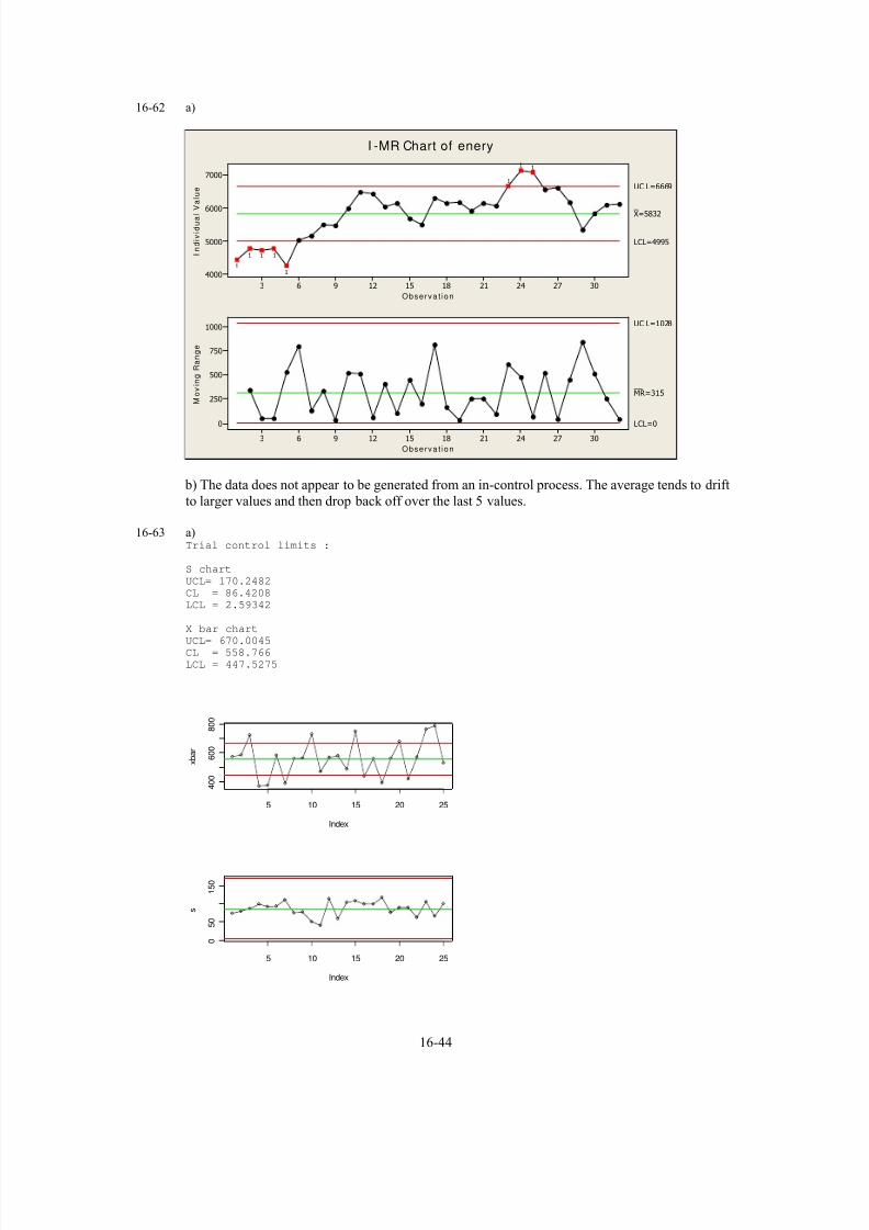
7/12/2019 Solution Manual Stats
http://slidepdf.com/reader/full/solution-manual-stats 576/588
16-62 a)
Observat ion
I n d i v i d u a l V a l u e
30272421181512963
7000
6000
5000
4000
_
X=5832
UC L=6669
LCL=4995
Observat ion
M o v i n g R a n g e
30272421181512963
1000
750
500
250
0
__ MR=315
UC L=1028
LCL=0
11
1
1
111
1
I -MR Chart of enery
b) The data does not appear to be generated from an in-control process. The average tends to drift
to larger values and then drop back off over the last 5 values.
16-63 a)Trial control limits :
S chart
UCL= 170.2482
CL = 86.4208
LCL = 2.59342
X bar chart
UCL= 670.0045
CL = 558.766
LCL = 447.5275
5 10 15 20 25
4 0 0
6 0 0
8 0 0
Index
x b a r
5 10 15 20 25
0
5 0
1 5 0
Index
s
16-44
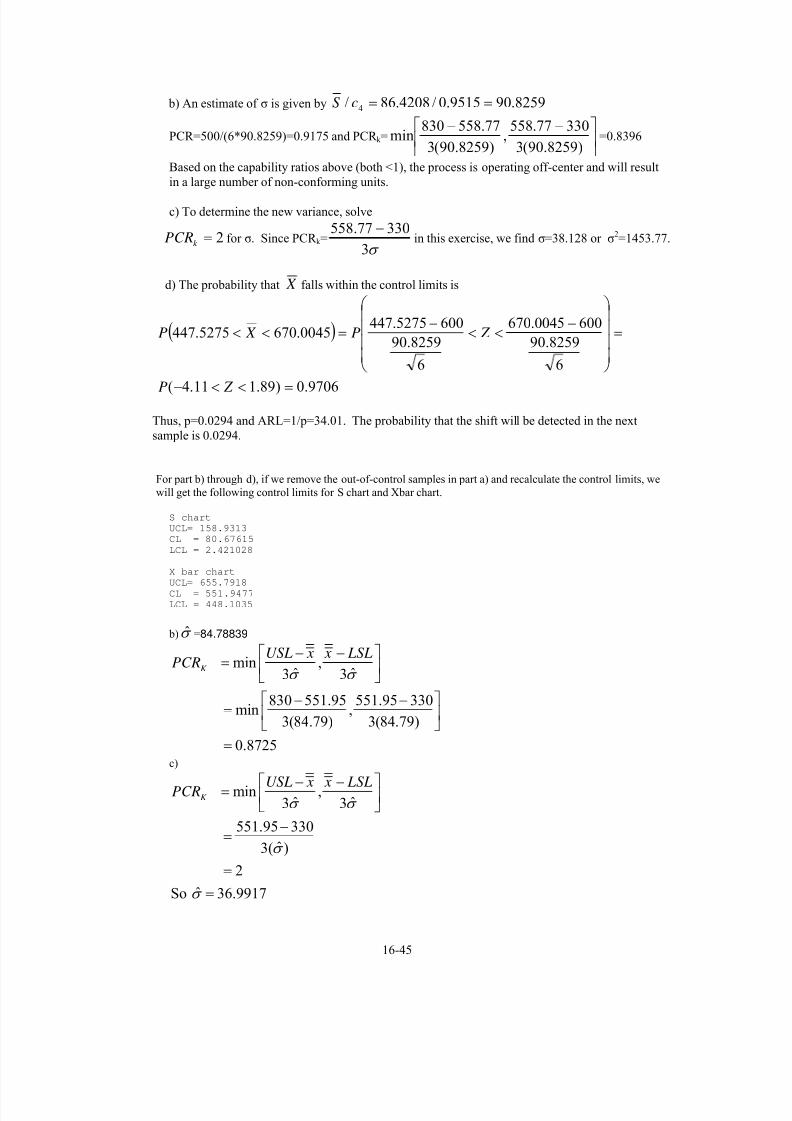
7/12/2019 Solution Manual Stats
http://slidepdf.com/reader/full/solution-manual-stats 577/588
b) An estimate of σ is given by 8259.909515.0/4208.86/ 4 ==cS
PCR=500/(6*90.8259)=0.9175 and PCR k = ⎥⎦
⎤⎢⎣
⎡ −−)8259.90(3
33077.558,
)8259.90(3
77.558830min =0.8396
Based on the capability ratios above (both <1), the process is operating off-center and will result
in a large number of non-conforming units.
c) To determine the new variance, solve
for σ. Since PCR 2=k PCR k =σ 3
33077.558 −in this exercise, we find σ=38.128 or σ2=1453.77.
d) The probability that X falls within the control limits is
( )
9706.0)89.111.4(
6
8259.90
6000045.670
6
8259.90
6005275.4470045.6705275.447
=<<−
=
⎟⎟⎟⎟
⎠
⎞
⎜⎜⎜⎜
⎝
⎛ −
<<−
=<<
Z P
Z P X P
Thus, p=0.0294 and ARL=1/p=34.01. The probability that the shift will be detected in the next
sample is 0.0294.
For part b) through d), if we remove the out-of-control samples in part a) and recalculate the control limits, we
will get the following control limits for S chart and Xbar chart.
S chart UCL= 158.9313
CL = 80.67615
LCL = 2.421028
X bar chart
UCL= 655.7918CL = 551.9477
LCL = 448.1035
b)σ ˆ =84.78839
min ,ˆ ˆ3 3
830 551.95 551.95 330min ,
3(84.79) 3(84.79)
0.8725
K
USL x x LSLPCR
σ σ
− −⎡ ⎤= ⎢ ⎥
⎣ ⎦
⎡ ⎤− −= ⎢ ⎥
⎣ ⎦=
c)
min ,ˆ ˆ3 3
551.95 330
ˆ3( )
2
ˆSo 36.9917
K
USL x x LSLPCR
σ σ
σ
σ
− −⎡ ⎤= ⎢ ⎥⎣ ⎦
−=
=
=
16-45

7/12/2019 Solution Manual Stats
http://slidepdf.com/reader/full/solution-manual-stats 578/588
d) In-control distribution X ~ N(551.9477, )234.6
Out-of-control distribution X ~ N(600, )234.6
P[448.1 ≤ X ≤ 655.8, when μ =600]
= ]6.346008.655
6.346001.448[ −≤≤− Z P
= ]6124.139.4[ ≤≤− Z P
=0.9463
Out-of-control ARL= =− 9463.01
118.6 ≈ 19.
16-64 ⎯ X Control Chart with 2-sigma limits
n LCL
nUCL
CL
σ μ
σ μ
μ
2,2 −=+=
=
02275.097725.01)2(1)2(2/
2
02275.097725.01)2(1)2(2/
2
=−=<−=−<=⎟⎟ ⎠
⎞⎜⎜⎝
⎛ −<
−=⎟
⎠
⎞⎜⎝
⎛ −<
=−=<−=>=⎟⎟ ⎠ ⎞⎜⎜
⎝ ⎛ >−=⎟
⎠ ⎞⎜
⎝ ⎛ +>
Z P Z Pn
X P
n X P
and
Z P Z Pn
X Pn
X P
σ
μ σ μ
σ
μ σ μ
The answer is 0.02275 + 0.02275 = 0.0455. The answer for 3-sigma control limits is 0.0027. The 3-sigma
control limits result in many fewer false alarms.
16-65
a) The following control chart use the average range from 25 subgroups of size 3 to estimate the process
standard deviation. Minitab uses a pooled estimate of variance as the default method for an EWMA control
chart so that the range method was selected from the options. Points are clearly out of control.
Sample
E W M A
24222018161412108642
64.7
64.6
64.5
64.4
64.3
64.2
64.1
64.0
63.9
_ _ X=64.1334
UCL=64.2759
LCL=63.9910
EWMA Char t of C3, ..., C5
16-46
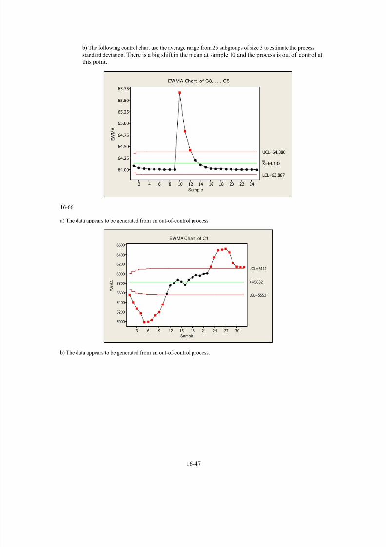
7/12/2019 Solution Manual Stats
http://slidepdf.com/reader/full/solution-manual-stats 579/588
b) The following control chart use the average range from 25 subgroups of size 3 to estimate the process
standard deviation. There is a big shift in the mean at sample 10 and the process is out of control at
this point.
Sample
E W M A
24222018161412108642
65.75
65.50
65.25
65.00
64.75
64.50
64.25
64.00
_ _ X=64.133
UCL=64.380
LCL=63.887
EWMA Chart of C3, . .., C5
16-66
a) The data appears to be generated from an out-of-control process.
Sample
E W M A
30272421181512963
6600
6400
6200
6000
5800
5600
5400
5200
5000
_ _
X=5832
UCL=6111
LCL=5553
EWMA Chart of C1
b) The data appears to be generated from an out-of-control process.
16-47

7/12/2019 Solution Manual Stats
http://slidepdf.com/reader/full/solution-manual-stats 580/588
Sample
E W M A
30272421181512963
7000
6500
6000
5500
5000
4500
_ _ X=5832
UCL=6315
LCL=5349
EWMA Chart of C1
16-67 a) The process appears to be in control.
Sample
E W M A
2018161412108642
60.3268
60.3267
60.3266
60.3265
60.3264
60.3263
60.3262
60.3261
_ _ X=60.32641
UCL=60.3267273
LCL=60.3260927
EWMA Chart of C1
b) The process appears to be in control.
Sample
E W M A
2018161412108642
60.32700
60.32675
60.32650
60.32625
60.32600
_ _ X=60.32641
UCL=60.326960
LCL=60.325860
EWMA Chart of C1
16-48

7/12/2019 Solution Manual Stats
http://slidepdf.com/reader/full/solution-manual-stats 581/588
16-68
Sample
C u m u l a t i v e S u m
30272421181512963
5.0
2.5
0.0
-2.5
-5.0
0
UCL=5.27
LCL=-5.27
CUSUM Chart of C1
Process standard deviation is estimated using the average moving range of size 2 with MR/d 2, where d 2 =
1.128. The estimate is 1.05. Recommendation for k and h are 0.5 and 4 or 5, respectively for n =1. For this
chart h = 5 was used.
16-69 The process is not in control.
K = k σ = 1, so that k = 0.5
H = hσ = 10, so that h = 5
40
30
20
10
0
-10
10
-10
20100
Subgroup Number
C u m u l a t i v e S u m
Upper CUSUM
Lower CUSUM
CUSUM Chart for hardness
16-49

7/12/2019 Solution Manual Stats
http://slidepdf.com/reader/full/solution-manual-stats 582/588
16-70
-80
0
80
-85.8529
85.8529
0 10 20
Subgroup Number
C u m u l a t i v e S u m
Upper CUSUM
Lower CUSUM
CUSUM Chart for Viscosity
Process standard deviation is estimated using the average moving range of size 2 with MR/d 2, where d 2 =
1.128 for a moving range of 2. The estimate is 17.17. Recommendation for k and h are 0.5 and 4 or 5,
respectively, for n = 1.
16-71 a)
Sample
C u m u l a t i v e S u m
24222018161412108642
0.020
0.015
0.010
0.005
0.000
-0.005
-0.010
0
UCL=0.01152
LCL=-0.01152
CUSUM Char t of x
σ is estimated using the moving range: 0.0026/1.128=0.0023. H and K were computed using
k=0.5 and h=5. The process is not in control.
b) EWMA gives similar results.
16-50

7/12/2019 Solution Manual Stats
http://slidepdf.com/reader/full/solution-manual-stats 583/588
Sample
E W M A
24222018161412108642
0.404
0.403
0.402
0.401
0.400
0.399
_ _ X=0.401184
UCL=0.403489
LCL=0.398879
EWMA Chart of x
16-72 a) Let p denote the probability that a point plots outside of the control limits when the mean has shifted from
μ0 to μ = μ0 + 1.5σ. Then,
5.0]0[5.0
)6()0()06(
3/
5.1
/3
/
5.1
33
)( 00
=−=
−<−<=<<−=
⎟⎟ ⎠
⎞⎜⎜⎝
⎛ +<
−<−
−=
⎟ ⎠
⎞
⎜⎝
⎛
+<<−=<<
Z P Z P Z P
nn
X
nP
n X nPUCL X LCLP
σ
σ
σ
μ
σ
σ
σ
μ
σ
μ
Therefore, the probability the shift is undetected for three consecutive samples is (1 − p)3 =
(0.5)3 = 0.125.
b) If 2-sigma control limits were used, then
15866.0]0[84134.01
)5()1()15(
2/
5.1
/2
/
5.1
22
)(1 00
=−−=
−<−−<=−<<−=
⎟⎟ ⎠
⎞⎜⎜⎝
⎛ +<
−<−
−=
⎟⎟ ⎠
⎞
⎜⎜⎝
⎛
+<<−=<<=−
Z P Z P Z P
nn
X
nP
n X nPUCL X LCLP p
σ
σ
σ
μ
σ
σ
σ
μ
σ
μ
Therefore, the probability the shift is undetected for three consecutive samples is (1 − p)3 = (0.15866)3 =
0.004.
c) The 2-sigma limits are narrower than the 3-sigma limits. Because the 2-sigma limits have a smaller
probability of a shift being undetected, the 2-sigma limits would be better than the 3-sigma limits for a mean
shift of 1.5σ. However, the 2-sigma limits would result in more signals when the process has not shifted
(false alarms).
16-51

7/12/2019 Solution Manual Stats
http://slidepdf.com/reader/full/solution-manual-stats 584/588
16-73. ARL = 1/ p where p is the probability a point falls outside the control limits.
a) μ μ and n = 1σ= +0
02275.0
]0[97725.01
1)4()2(
)3()3(
/
3
/
3
)()(
0000
=
+−=
=−<+>=
−−<+−>=
⎟⎟⎟⎟
⎠
⎞
⎜⎜⎜⎜
⎝
⎛ −−−
<+⎟⎟⎟⎟
⎠
⎞
⎜⎜⎜⎜
⎝
⎛ −−+
>=
<+>=
nwhen Z P Z P
n Z Pn Z P
n
n
Z Pn
n
Z P
LCL X PUCL X P p
σ
σ μ σ
μ
σ
σ μ σ
μ
Therefore, ARL = 1/ p = 1/0.02275 = 43.9.
b) μ μ σ= +0 2
15866.0
]0[84134.01
1)5()1(
)23()23(
/
23
/
23
)()(
0000
=
+−=
=−<+>=
−−<+−>=
⎟⎟⎟⎟
⎠
⎞
⎜⎜⎜⎜
⎝
⎛ −−−<+
⎟⎟⎟⎟
⎠
⎞
⎜⎜⎜⎜
⎝
⎛ −−+>=
<+>
nwhen Z P Z P
n Z Pn Z P
n
n Z P
n
n Z P
LCL X PUCL X P
σ
σ μ σ
μ
σ
σ μ σ
μ
Therefore, ARL = 1/ p = 1/0.15866 = 6.30.
c) μ μ σ= +0 3
50.0
]0[50.01
1)6()0(
)33()33(
/
33
/
33
)()(
0000
=+−=
=−<+>=
−−<+−>=
⎟⎟⎟⎟
⎠
⎞
⎜⎜⎜⎜
⎝
⎛ −−−<+
⎟⎟⎟⎟
⎠
⎞
⎜⎜⎜⎜
⎝
⎛ −−+>=
<+>
nwhen Z P Z P
n Z Pn Z P
n
n Z P
n
n Z P
LCL X PUCL X P
σ
σ μ σ
μ
σ
σ μ σ
μ
Therefore, ARL = 1/ p = 1/0.50 = 2.00.
d) The ARL is decreasing as the magnitude of the shift increases from σ to 2σ to 3σ. The ARL decrease as
the magnitude of the shift increases since a larger shift is more likely to be detected earlier than a smaller
shift.
16-52
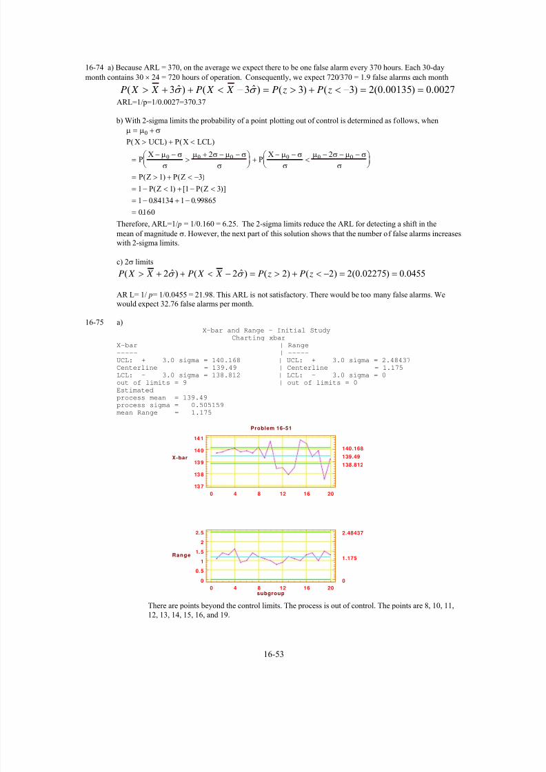
7/12/2019 Solution Manual Stats
http://slidepdf.com/reader/full/solution-manual-stats 585/588
16-74 a) Because ARL = 370, on the average we expect there to be one false alarm every 370 hours. Each 30-day
month contains 30 × 24 = 720 hours of operation. Consequently, we expect 720/370 = 1.9 false alarms each month
0027.0)00135.0(2)3()3()ˆ3()ˆ3( ==−<+>=−<++> zP zP X X P X X P σ σ
ARL=1/p=1/0.0027=370.37
b) With 2-sigma limits the probability of a point plotting out of control is determined as follows, when
μ μ σ= +0
P X UCL P X LCL
PX
PX
P Z P Z
P Z P Z
( ) ( )
( ) ( )
( ) [ ( )]
. .
.
> + <
=− −
>+ − −⎛
⎝ ⎜⎞ ⎠⎟
+− −
<− − −⎛
⎝ ⎜⎞ ⎠⎟
= > + < −
= − < + − <
= − + −
=
μ σ
σ
μ σ μ σ
σ
μ σ
σ
μ σ μ σ
σ0 0 0 0 0 02 2
1 3
1 1 1 3
1 084134 1 0 99865
0160
Therefore, ARL=1/ p = 1/0.160 = 6.25. The 2-sigma limits reduce the ARL for detecting a shift in the
mean of magnitude σ. However, the next part of this solution shows that the number of false alarms increases
with 2-sigma limits.
c) 2σ limits
0455.0)02275.0(2)2()2()ˆ2()ˆ2( ==−<+>=−<++> zP zP X X P X X P σ σ
AR L= 1/ p= 1/0.0455 = 21.98. This ARL is not satisfactory. There would be too many false alarms. We
would expect 32.76 false alarms per month.
16-75 a)X-bar and Range - Initial Study
Charting xbar
X-bar | Range
----- | -----
UCL: + 3.0 sigma = 140.168 | UCL: + 3.0 sigma = 2.48437
Centerline = 139.49 | Centerline = 1.175
LCL: - 3.0 sigma = 138.812 | LCL: - 3.0 sigma = 0
out of limits = 9 | out of limits = 0
Estimated
process mean = 139.49process sigma = 0.505159
mean Range = 1.175
0 4 8 12 16 20
13 7
13 8
13 9
14 0
14 1
139.49
140.168
138.812
0 4 8 12 16 20
0
0.5
1
1.5
2
2.5
1.175
2.48437
0
X-bar
Problem 16-51
subgroup
Range
There are points beyond the control limits. The process is out of control. The points are 8, 10, 11,
12, 13, 14, 15, 16, and 19.
16-53

7/12/2019 Solution Manual Stats
http://slidepdf.com/reader/full/solution-manual-stats 586/588
b) Revised control limits are given in the table below:
X-bar and Range - Initial Study
Charting Xbar
X-bar | Range
----- | -----
UCL: + 3.0 sigma = 140.417 | UCL: + 3.0 sigma = 2.595682
Centerline = 139.709 | Centerline = 1.227273LCL: - 3.0 sigma = 139.001 | LCL: - 3.0 sigma = 0
out of limits = 0 | out of limits = 0
1050
140.5
140.0
139.5
139.0
Subgroup Number
x b a r
Xbar Chart
Mean=139.7
UCL=140.4
LCL=139.0
1050
3 .0
1 .5
0
S u b g r o u p N u m b e r
r
R C hart
M ean=1.227
U C L = 2 . 5 9 6
L C L = 0
There are no further points beyond the control limits.
The process standard deviation estimate is given by 5276.0326.2
227273.1ˆ
2
===d
Rσ
c) 26.1)528.0(6
138142
ˆ6=
−=
−=
σ
LSLUSLPCR
[ ] 08.108.1,45.1min
)528.0(3
138709.139,
)528.0(3
709.139142min
ˆ3,
ˆ3min
==
⎥⎦
⎤⎢⎣
⎡ −−=⎥
⎦
⎤⎢⎣
⎡ −−=
σ σ
LSL x xUSLPCRk
Because the process capability ratios are less than unity, the process capability appears to be poor. PCR is
slightly larger than PCR k indicating that the process is somewhat off center.
16-54

7/12/2019 Solution Manual Stats
http://slidepdf.com/reader/full/solution-manual-stats 587/588
d) In order to make this process a “six-sigma process”, the variance σ2would have to be decreased such that
PCR k = 2.0. The value of the variance is found by solving PCR k = 0.23
=−
σ
LSL xfor σ:
2848.0
6
138709.139
138709.1396
0.23
138709.139
=
−=
−=
=−
σ
σ
σ
σ
Therefore, the process variance would have to be decreased to σ2= (0.2848)
2= 0.081.
e) σx= 0.528
8197.0
093418.0913085.0
)32.1()36.1(
)35.132.1(528.0
7.139417.140
528.0
7.139001.139
)7.139|417.140001.139(
=
−=
−<−<=
<<−=
⎟⎟
⎠
⎞⎜⎜
⎝
⎛ −<
−<
−=
=<<=
Z P Z P
Z P
X P
X P p
xσ
μ
μ
The probability that this shift will be detected on the next sample is 1 − p = 1−0.8197 = 0.1803.
55.51803.0
1
1
1==
−=
p ARL
16-76
a) The probability of having no signal is
( 3 3) 0.9973P X − < < = P(No signal in 3 samples)=(0.9973)
3=0.9919
P(No signal in 6 samples)=(0.9973)6= 0.9839
P(No signal in 10 samples)=(0.9973)10= 0.9733
16-77 PCR = 2 but μ σ = +USL 3
P X USL P Z P Z( )( )
( ) .< = <− −⎛
⎝ ⎜
⎞ ⎠⎟ = < − =
μ σ μ
σ3
3 0 00135
16-78 a) The P(LCL < < UCL), when p = 0.08, is needed.P
115.0100
)05.01(05.0305.0
)1(3
0015.0
100
)05.01(05.0305.0
)1(3
=−
+=−
+=
→−=−
−=−
−=
n
p p pUCL
n
p p p LCL
Therefore, when p = 0.08
16-55

7/12/2019 Solution Manual Stats
http://slidepdf.com/reader/full/solution-manual-stats 588/588
100
)92.0(08.0
08.0115.0
100
)92.0(08.0
08.0ˆ)115.0ˆ()115.0ˆ0(
⎟⎟⎟⎟
⎠
⎞
⎜⎜⎜⎜
⎝
⎛ −
≤−
=≤=≤≤P
PPPPP