solution techniques for large … techniques for large eigenvalue problems in structural-etclul ......
TRANSCRIPT

SOLUTION TECHNIQUES FOR LARGE EIGENVALUE PROBLEMS IN STRUCTURAL-ETClUlJU 79 1 LEE, A R ROBINSON NOOO1-7S-C-01
UCLASSIFIEO UILU-EG79-2006 NL
.9 m/IEIIEI/IE.Ell/EllEl/lEEI//////EEEI/IIEEIIEEEIIIIEIIEIEEEI/IIII/IIIIIfllfflfflffllfllfEhEII/EII/IIIIE

1150 11111
IlitE lll iIIII-
1.JI 25 IIHI 4 1111.6
MICROCOPY RESOLUTION TEST CHART
NATIONAL HIUREAU OF STANDARDS 1964

CM"L UNGIEERNG STUDIES"I -vRam -m US No. 4u
SOLUION TECroHNIQUES FOR LARGE EIGEN VALUEPROBLE M IN STRUCTURAL DYNAMICS
U LEYEk-- I.-W. LEE
A fosnWc Rbpot ofReseod Spenasrid by
- INTH OFFIC OF NAVAL RESEARCHDEPARTMENT OF THE NAVY
- Cont~rac No, N00014-75.C-016Prolec No, NW W&4183
- Seprbducllofn Mn vwo or Mn paff is pa M!te
I ~~fwoWm prpom of &he Unitd Sts Gvowermn.
Aproved for Public Releass DWAtrbufto Unlimited
atUUANA-a4AMPAIGNLURBANA, IWNOIS
1JUNE 1979
1.1022

s'n -I a
( Solution Techniques f or Large Elgenvalue Problems in ,
Strctra Dynamics.Rbno
Department of Civil Engineering 04-8Universityemr oiif Illinois at Urbana-Champaign _.. ....- ":-"-- "
NwakCvlEngineering Laboratory 001-5-16!208 N. Romine Street )
nMaterial Science Division
Structural Mechanics Program (code 474) Technical .ept j
Off ice of Naval Research (800 Quincy Street) HArlington, Virginia 22217
tu Supp-ims a0y oe
Dep~ AatLmet o00 Cii Egnerngn)-
This study treats the determination of eigenvalues and eigenvectors of largealgebraic systems. The methods developed are applicable to finding the naturalfrequencies and modes of vibration of large structural systems.
For distinct eigenvalues the method is an application of the modified Newton-
Raphson method that turns out to be more efficient than the standard competingschemes.
For close or multiple eigenvalues, the modified Newton-Raphson method is generalizeto form a new process. The entire set of close eigenvalues and their eigenvectorsare found at the same time in a two-step procedure. The subspace of the approximateeigenvectors is first projected onto the subspace of the true eigenvectors. If theeigenvalues are multiple, the results of the first stage indicate this fact and theprocess terminates. If they are merely close, a single rotation in the newly foundspace solves a small eigenvalue problem and provides the final results for the closeset. The procedure for subspace projection can be expressed as a simple extremum
problem that generalizes the known extremum property of eigenvectors.
Computational effort and convergence are studied in three example problems. Themethod turns out to be more efficient than subspace iteration.
17. Documew Amnaems a. Doulptom
EigenvaluesEigenvectorsNumerical AnalysisDynamic Structural Analysisb. Idantffee/Oan4ndad Tern
c. COSATI FIeld/Group
I. Availablifty Snta a 1%, Securit Clam (Thi sort) 21. Ne. of Peoa
Approved for public release: Distribution Unclassified 118unlimited 2. Securt Cam (me Peu) I3. PrimaUnrl-sifi4 or
(SSANSI-a9.11) 8 Inatuetln a Revrm OPTHMM V. . (4--
(Formety TSS)" "-1/ /o
.. "I - ,-

1. SOLUTION TECHNIQUES FOR LARGE EIGENVALUE
-- PROBLEMS IN STRUCTURAL DYNAMICS
by
I.-W. Lee
A. R. Robinson
mm
* -A Technical Report of
Os Research Sponsored by
THE OFFICE OF NAVAL RESEARCH-- DEPARTMENT OF THE NAVY
Contract No. N00014-75-C-0164
Project No. NR 064-183
Reproduction in while or in part is permittedfor any purpose of the United States Government.
& Approved for Public Release: Distribution Unlimited
II at Urbana-Champaign
Urbana, Illinois
June 1979
I

iii
ACKNOWLEDGMENT
This report was prepared as a doctoral dissertation by
, • Mr. In-Won Lee and was submitted to the Graduate College of the
- University of Illinois at Urbana-Champaign in partial fulfillment of
i j the requirements for the degree of Doctor of Philosophy in Civil
* Engineering. The work was done under the supervision of
Dr. Arthur R. Robinson, Professor of Civil Engineering.
The investigation was conducted as part of a research program
-, - supported by the Office of Naval Research under Contract N00014-75-C-
0164, "Numerical and Approximate Methods of Stress Analysis."
The authors wish to thank Dr. Leonard Lopez, Professor of
Civil Engineering, for his assistance.
The numerical results were obtained with the use of the
CYBER-75 computer system of the Office of Computer Services of the
University of Illinois at Urbana-Champaign.
Access'"~ F~or_-
D itributfl
I
I
if
.o_ ~~~~~t codesllJIN u .,,- Ill I I m l i i ,n ' -

TABLE OF CONTENTS
Page
1. INTRODUCTION ......... ........................... 1
1.1 General ....... .. ........................... I1.2 Object and Scope ........ ...................... 21.3 Review of Solution Methods ...... ................. 31.4 Notation .......... .......................... 6
2. DISTINCT ROOTS ...... ......................... .... 10
2.1 General ... .......................... 102.2 The Iterative Scheme ....... .................... 102.3 Convergence Rate and Operation Count .... ............ 142.4 Errors in Approximate Eigensolutions .... ............ 172.5 Treatment of Missed Eigensolutions ................ ... 19
3. CLOSE OR MULTIPLE ROOTS ..... ..................... ... 21
3.1 General ....... .......................... .. 21*0 3.2 Theoretical Background ....... ................... 22
3.3 The Iterative Scheme ........ .................... 253.4 Treatment of Close Roots ... .................. 303.5 Convergence Rate and Operation Count .... ............ 31
" 4. APPROXIMATE STARTING EIGENSOLUTION ...... ............... 34
4.1 General ..... .......................... 344.2 Subspace Iteration Method ................. 35
4.2.1 The Iterative Scheme .... ................ ... 354.2.2 Starting Vectors ....... .................. 374.2.3 Convergence Rate, Operation Count, and
Estimation of Errors ......... ... .... 384.3 Starting Solution for the Proposed Method .... ......... 41
5. NUMERICAL RESULTS AND COMPARISONS .... ................ ... 43
5.1 General ....... .......................... .. 435.2 Plane Frame ....... ........................ ... 445.3 Arch ........ ............................ .. 455.4 Plate Bending ........ ....................... 465.5 Comparison between the Theoretical Convergence Rates and
Numerical Results ........ ..................... 47
6. SUMMARY AND CONCLUSIONS ....... ..................... 49
1 6.1 Summary of the Proposed Method ..... ............... 496.2 Conclusions .......................... 506.3 Recommendations for Further Study ............. 51
'i ... .I I I ( I m ._ ". - - - ... r

v
i
Page
LIST OF REFERENCES ....... ......................... ... 52
APPENDIX
A. NONSINGULARITY OF THE COEFFICIENT MATRICES OFTHE BASIC EQUATIONS ........ .................... 57
B. CONVERGENCE ANALYSIS ....... .................... 61
B.1 Case of a Distinct Root .... ............... ... 61B.2 Case of a Multiple Root .... ............... ... 67
C. THE BASIC THEOREMS ON THE CONSTRAINEDSTATIONARY-VALUE PROBLEM ..... .................. .. 77 -
' q1
t. j
I
I
. K

[ilii vi
LIST OF TABLES
Table Pagei,.
1 1. NUMBER OF OPERATIONS FOR EIGENSOLUTIONS ............... .. 86
2. EIGENVALUES OF THE PLANE FRAME PROBLEM (DISTINCT ROOTS) ..... .. 90
3. EIGENVALUES OF THE CIRCULAR ARCH PROBLEM (DISTINCT ROOTS) . ... 92
4. EIGENVALUES OF THE SQUARE PLATE PROBLEM (DOUBLE ROOTS) ..... .. 94
5. EIGENVALUES OF THE RECTANGULAR PLATE PROBLEM (CLOSE ROOTS) . . .95
* 6. COMPARISON OF THE TOTAL NUMBER OF OPERATIONS .... .......... 96
7. COMPARISON BETWEEN THE THEORETICAL CONVERGENCE RATES FOR
• . EIGENVECTORS AND THE NUMERICAL RESULTS - FRAME PROBLEM(DISTINCT ROOTS) ...... ........................ .. 97
8. COMPARISON BETWEEN THE THEORETICAL CONVERGENCE RATES FOR* "EIGENVECTORS AND THE NUMERICAL RESULTS - SQUARE PLATE
PROBLEM (DOUBLE ROOTS) ..... ..................... ... 98
S"9. NUMERICAL CONVERGENCE RATES FOR EIGENVECTORS -RECTANGULAR PLATE PROBLEM (CLOSE ROOTS) ............... .. 99
i
III*1

I. vi iLIST OF FIGURES
Figure Page
1. ESTIMATION OF ERRORS IN APPROXIM.TE EIGENVECTORS ..... ... 100
- 2. TEN-STORY, TEN-BAY PLANE FRAME ................ .... 101
° _.
T
Ii
- -S *4"

I.-
,- 1. INTRODUCTIONa.
1.1 General
-. Various engineering problems can be reduced to the solution of matrix
" eigenvalue problems. Typical examples in the field of structural engineeringare the problem of determination of natural frequencies and the corresponding
normal modes in a dynamic analysis and the problem of finding buckling loads
in a stability analysis of structures. Since the advent of the digital com-
. puter, the complexity of structures which can be treated and the order of
the corresponding eigenvalue problems have been greatly increased. Hence,
" "the development of solution techniques for such problems has attracted much
attention.
For the dynamic analysis of a linear discrete structural system by
*superposition of modes, we must first solve the problem of free vibration
*of the system. The free vibration analysis of the linear system without
I "damping reduces to the solution of the linear eigenvalue problem
I. Ax = x 3x (1.1)
I. in which A and B are stiffness and mass matrices of order n, the number of
degrees of freedom of the structural system. A column vector x is an
eigenvector (or normal mode), and the scalar x the corresponding eigenvalue
(or the square of a natural frequency).
The matrices A and B are real and synmetric, and are usually banded and
sparse. If a consistent mass matrix is used, the matrices A and B have the
Le* ,
2
same bandwidth [4,5]. If a lumped mass model of the system is used, B will
be diagonal. The matrix B is positive definite, but the matrix A may be
semidefinite. There are n sets of solutions of Eq. (1.1), that is, n eigen-
values and their corresponding eigenvectors.
Frequently, in practical eigenvalue problems, the order of A and B is
so high that it is impractical or very expensive to obtain the complete
eigensolution. On the other hand, to carry out a reasonably accurate
dynamic analysis of the structure, it is possible to consider only a partial
eigensolution. The partial solution of interest may consist of only few
lowest eigenvalues and their eigenvectors, or eigenvalues in the vicinity
of a given frequency and the corresponding eigenvectors. The method
described in this study is aimed at effective solution of this type of
problem rather than at a complete eigensolution.
1.2 Object and Scope
The object of this study is to present an iterative method which is
efficient and numerically stable for the accurate computation of limited
number of eigenvalues and the corresponding eigenvectors of linear eigenvalue
problems of large order.
The method developed remedies the major drawbacks of the inverse iter-
ation method with spectral shifting [13]: numerical instability due to
shifting and slow convergence when eigenvalues are equal or close in magni-
tude. The proposed method converges rapidly and is numerically stable for any
number of multiple or close eigenvalues and the corresponding etgenvectors.
4 '

Im
.3 3
The procedure for distinct eigenvalues is treated in Chapter 2, and a
modified procedure for multiple or close eigenvalues in Chapter 3. SelectionU.
of initial approximate eigenvalues and eigenvectors by the subspace iteration
.* method is described in Chapter 4. To show the efficiency of the proposed
. method, three sample problems are solved: vibration of a plane frame, of
a plate in bending, and of an arch. Comparisons are made in Chapter 5 with
a method which is generally regarded as very efficient, the subspace
iteration method.
1.3 Review of Solution Methods
- -Numerous techniques for the solution of eigenvalue problems have been
developed. These techniques can be divided into two classes - techniques
for approximate solution and techniques for "exact" solution.
The approximate solution techniques include well-known static conden-
- - sation [2,3,24,25,27,42], dynamic condensation [34], Rayleigh-Ritz analysis
[9,13,31,48], component mode analysis and related methods summarized by
Uhrig [50]. These methods are essentially techniques for reducing the size
of a system of equations. The reduction of a system of equations eventually
1leads to a loss in accuracy of a solution. However, the advantage of
lessened computational effort for a solution sometimes may compensate for
the loss in accuracy. Moreover, an approximate solution found by these methods
may serve as the starting solution for the exact methods, which will be
discussed next.
The exact methods are designed for the accurate computation of some
or all the eigenvalues and corresponding eigenvectors. These methods consistII'K_ i - - -mr: . _ . _ ' _ '

4
of vector iteration methods, transformation methods, the method based on
the Sturm-sequence property, polynomial iteration method, and minimization
methods. These methods are well described in Ref. 51. The methods differ
in the choice of which mathematical properties of an eigenvalue problem are
used. The vector iteration methods such as the classical vector iteration
(power method) and simultaneous vector iteration deal with the form of
equations Ax = x Bx. The transformation methods (LR, QR, Jacobi, Givens,
and Householder methods) are based on the mathematical property that the
eigenvalues of a system are invariant under similarity transformations. In
the polynomial iteration method, the roots of det (A - XB ) = 0 are found,
and minimization methods are based on the stationary property of the
Rayleigh quotient [43].
In vector iteration methods and minimization methods, both the eigen-
values and corresponding eigenvectors are found simultaneously, but in
other exadct methods, only eigenvalues are computed or the computed eigen-
vectors are, in general, not suitable for use in the final solutions. In
such methods, another method such as the vector iteration method with a
shift may be used for finding the eigenvector corresponding to a computed
eigenvalue.
For a limited number of eigenvalues and corresponding eigenvectors of
an eigenvalue problem of large order which we are concerned with in this
study, the above methods have been modified or combined to take advantage
of the useful characteristics of several of the methods. First, the
determinant search method [7,9,22,23] combines the methods based on the Sturm-
sequence property, polynomial iteration, and inverse iteration. In this
t.

5
method, eigenvalues in a specified range are approximately isolated by using
the bisection method and the Sturm-sequence property and then located
accurately by the polynomial iteration method. The corresponding eigen-
vectors are computed by inverse iteration with a shift. By this method,
eigenvalues in any range and corresponding eigenvectors can be found.
However, it has the disadvantage that the matrix is factorized in each iter-
ation to locate the eigenvalues of interest.
Another method for the solution of large eigenvalue problems is the
so-called subspace iteration method [6,15,32,39,47], which is a combination
of the simultaneous iteration method and a Rayleigh-Ritz analysis. in this
method, several independent vectors are improved by vector inverse iteration,
and the best approximation to the eigenvectors are found in the subspace of
the iteration vectors by a Rayleigh-Ritz analysis. In this method, eigen-
values at the end of the spectrum and the corresponding eigenvectors converge
very rapidly. This method will be discussed further in Chapter 4.
The inverse iteration method with a shift is known to be extremely
efficient for improving approximate eigenvalues and eigenvectors. However,
as mentioned in the previous section, when the shift is very close to a true
eigenvalue, the method exhibits numerical instability, yielding unreliable
answers [13]. In addition, when the eigenvalues of interest are close to-
gether, their convergence is very slow. Robinson and Harris [44] developed
an efficient method to overcome the above difficulty for distinct eigenvalues
(: I by augmenting ihe equations used in the inverse iteration method by a side
S mequation. While this method extracts eigenvalues and eigenvectors simul-
taneously with a very high convergence rate, it has the disadvantage that the

6
algorithm is inefficient for problems with multiple or close eigenvalues.
This method and some improvements on it will be discussed further in the
next chapter.
1.4 Notation
All symbols are defined in the text when they first appear.
With regard to matrices, vectors, elements of matrices or vectors, and
iteration steps, the following conventions are generally used:
(1) Matrices are denoted by uppercase letters, as A, B and X.
(2) A column vector is denoted by a lowercase letter with a
superior bar and a subscript, as aj, b. and x.(3) Elements of a matrix or vector are denoted by a lowercase
letter with a double subscripts, as aij, bi. and xi.
(4) Iteration steps are denoted by a superscript, as X(k), i(k)
and x k13(5) k) (k)(5) Increments are denoted by the symbol A, as Ax. and Ax..
j ij
Some symbols are assigned more than one meaning. However, in the context
of their use there are no ambiguities.
A, aj, aij stiffness matrix, jth column vector of A, element
of A
A*(k) projection of A onto the subspace spanned by vectors
in y(k) A*(k) = y(k)T A y(k)
a = radius of circular arch
B, bj, b = mass matrix, j th column vector of B, element of B
B(k) projection of B onto the subspace spanned by vectors
in y(k), B*(k)= Y(k)T B y(k)
tIj"

P
-. 7
c (k). E(k) Cik) = expansion matrix of X(k), jth column vector of
element of C(k), X(k) = XC(k)
D = diagonal matrix, see Section 2.2
-Q De = plate bending stiffness, De = EH3/12(l-u 2)
D, (. = matrix for finding close or multiple eigenvalues and
eigenvectors, jth column vector of D, see Eq. (3.24)
D(k), (T(k) = iteration matrix for D after k iterations, jth column
vector of D(k), see Eq. (3.23)
E = Young's modulus
E, ej, e = diagonal matrix, jth column vector of E, element of
E, see Eq. (A.7)
e., e diagonal matrix, jth column vector of E , element of
E*, E* =-E1
h thickness of plate
= number indicating rate of convergence of eigenvector,
see Eq. (2.13)
I =moment of inertia of cross-section
Is = identity matrix of order s
i, j = indices of matrix elements
k = superscript indicating number of iterations
L lower triangular matrix
= Lagrangian, see Eq. (3.6)
ma, Mb = average half bandwidth of A, of B
Np, Nr, Ns = total number of operations required for finding
eigenpairs by the proposed method, by the Robinson-
Harris method, by the subspace-iteration method
W A"A6
I ia, *
8
n = order of A and B
p = number of eigenpairs sought
q = number of iteration vectors by subspace iteration
method, q = max(2p, p+8)
-(k) residual vector of approximation to jth eigenpair
after k iterations
s = number of close and/or multiple eigenpairs sought
Tp, Tr, Ts = number of iterations needed to find eigenpairs by
proposed method, by Robinson-Harris method, by
subspace iteration method
X, j, xi matrix of eigenvectors (modal matrix), ith eigen-
vector, element of X
X(k), i(k) , xlk) = approximation to X after k iterations, jth column
vector of X(k) , element of X(k)
y(k), _(k), (k) = matrix of iteration vectors improved from X(k) by
simultaneous iteration method, jth column vector of
y(k), element of y(k)
Z, z(k) = rotation matrix, approximation to Z after k iterations
y(k) = error in X(k) or (k)J J "jj
= increment operator
6ij = Kronecker delta
e(k) = error In R(k) or -(k)
X M multiple eigenvalue
A, A = diagonal matrix of eigenvalues, jth eigenvalue,
A =diag(XI , X2, X ., I
~F
-.

L 9A(k) X(k) =approximation to A, to X., after k iterations
p= shift applied in vector iteration method
12ij vii' = element of D, of D (k)
p = mass density
= natural circular frequency, X w2

10
2. DISTINCT ROOTS
2.1 General
In this chapter, a method for finding a simple eigenvalue and the
corresponding eigenvector will be presented. The method developed by
Robinson and Harris [44] is modified here to save overall computational
effort for finding an eigensolution. The Robinson-Harris method is an
application of the Newton-Raphson technique for improving the accuracy of
an approximate eigenvalue and the corresponding approximate eigenvector.
In the proposed mEthod, a modified form of the Newton-Raphson technique is
applied instead of the standard one used in the Robinson-Harris method.
In Section 2.2, the Robinson-Harris method will be discussed first;
then the proposed method will be presented. The convergence rate of the
proposed method and the number of operations per iteration will be given in
Section 2.3. The estimation of error in an approximate solution is found
in Section 2.4. A technique for the examination of the converged solution
to determine whether the eigenvalues and corresponding eigenvectors of
interest have been missed and a method for finding a missed solution will
be presented in Section 2.5.
2.2 The Iterative Scheme
Let us consider the following linear eigenvalue problem&
A = AjB~ (j = 1, 2, . . , n) (2.1)
[[I,

IF
4
where A and B are assumed to be given symmetric matrices of order n and B
is taken to be positive definite. The A. and i. are the jth eigenvalue and
the corresponding eigenvector.
Let us assume that an initial approximate solution of Eq. (2.1), Xj(0)
and i*(O) is available. Denote an approximate eigenvalue and the corre-
sponding eigenvector after k iterations by X and (k = 0, 1, .
Then, we have
Ai(k) _ (k) Bij(k) = rj(k) (2.2)
where j(k) is a residual vector.
The object is to remove the residual vector in Eq. (2.2). The Newton-
Raphson technique is applied for this purpose. Let the (k + 1)th approxi-
mation be defined by
(k+1) = X (k) + AX (k)
(k+1) = -j(k) + Aj (k) (2.3)
x x (23
where Axj (k) and Ax ) are small unknown incremental changes of X (k) and
xj ( k ) . Substituting xj(k+ ) and x j(k+) of Eq. (2.3) for Xi and x in
Eq. (2.1) and discarding a nonlinear term AX (k). BAx(k) as very small
compared with the other, linear, terms, we get
(A - A(k)B) Ax(k) - AA.(k) Bx(k ) = - .(k) (2.4)j~ 3 3 3
where (k) is the residual vector defined in Eq. (2.2).
j.

12
Note that in Eq. (2.4), there are n+1 scalar unknowns (k) and n
components of Axj(k)), but only n equations. Hence, it is required for the
solution of Eq. (2.4) that either the number of unknowns be reduced or one
equation added. Derwidue [16] and Rall [41] reduced the number of unknownsby setting the nth component of the vector AR (k) or x (k+1) at a preassigned
value - zero or one. In these methods, it may happen that an unfortunate
choice of one component results in failure of the procedure.
Instead of reducing the number of unknowns, Robinson and Harris [44]
added an extra equation (side condition) to the system of Eq. (2.4), to
arrive at a set of n+1 equations in n+1 unknowns. This side condition is
(k) T (k) (x BAR 0(2.5)
Equation (2.5) means that the incremental value Ax(k) is orthogonal to
the current approximate eigenvector Rj(k) with respect to the matrix B.
The side condition prevents unlimited change in the ij(k). The resulting
set of simultaneous linear equations may be written in matrix form as
A- (k)B _Bx (k) - (k) _ (k)
. .. (2.6)
-x. B 0 (k) 03 B
where the residual vector is given in Eq. (2.2). The coefficient
matrix for the incremental values is of order n+1 and symmetric. Moreover,
it is nonsingular if x is not multiple [44]. Equation (2.6) may be solved
for Axj(k) and Ax(k) by Gauss elimination, or by any other suitablefor 3te uia
I

A- 13
:.
technique. Note that the submatrix in the coefficient matrix (A - (k)B)tehiqe Noeta3h
(k)is almost singular when A. is close to A. However, this does not cause
any difficulty in solving Eq. (2.6), since in the elimination process only
- - the last pivot element, in general, becomes very small. Thus, the inter-
change of columns and rows does not increase significantly the column height-(k+l) -j(k+l)of the factorized matrix. The improved values, A. and x , are
computed from Eq. (2.3). The procedure employing Eqs. (2.3) and (2.6) is
repeated until the errors in the A.(k) and Rj(k) are within allowable toler-
- ances. The method of estimating these errors will be discussed in Sec-
""n tion 2.4.
", The convergence of the above process for an eigenvalue and the corre-
sponding eigenvector has been shown to be better than second order; the
order has been found to be 2.41 [44]. However, the algorithm using Eq. (2.6)
requires a new triangularization in each iteration, since the values of the
* telements of the coefficient matrix are changed in each iteration as a result
of hagig fomA.(k) (k+1)of changing from to j l The number of operations (multiplications
and divisions) required in such a triangularization is very large.
I To avoid the complete elimination procedure in each iteration, the
following equations instead of Eq. (2.6) are used in the proposed method.
[A - A- (k) Aj(k) - j(k)
• (2.7)
k • B 0 1 A (k) J30
II

14
where the residual vector r(k) is defined in Eq. (2.2). Equation (2.7)
was obtained by introducing Eq. (2.3) into Eq. (2.1) and discarding a small
linear term (x.(k+ ) - A i(O) BAj(k). Note that Eq. (2.7) differs from
Eq. (2.6) in such a way that the coefficient matrix in Eq. (2.6) has the
submatrix (A - xj(k)B), while the coefficient matrix in Eq. (2.7) has
(A - A O)B). The coefficient matrix in Eq. (2.7) is also symmetric, and
nonsingular if x. is not multiple. The nonsingularity of the coefficient
matrix will be proved in passing, in Appendix A.
From the form of the coefficient matrix, it can be seen that once the
matrix is decomposed into the form LDLT, where L is lower triangular and D
is diagonal, only a small number of additional operations is required
for the solution of Eq. (2.7) in the succeeding iterations, since only the
vector BRj(k) in the matrix is changed in each iteration. The proposed
method therefore considerably reduces the number of operations required in
each iteration. On the other hand, the method lowers the convergence rate
because of the neglect of the small linear term (x. (k+1) _ Aj (0) (BAxj(k))
which in turn increases the number of iterations for a solution. However,
the overall computational effort for a solution does decrease. It will be
seen in Chapter 5 that the proposed method is actually more efficient than
the Robinson-Harris method.
2.3 Convergence Rate and Operation Count
The efficiency of a numerical method such as the one proposed here can
be estimated given the convergence rate and the number of operations per
iteration required in the process. The convergence analysis, which is given
I.

U. 15
in Appendix B, will be summarized as follows. Let an approximate eigenvector
(k) be expanded in terms of the true eigenvectors xi, i.e.,ma
nj(k) = (k) (_ ci xi (2.8)
i" i
where c.(k) is a coefficient of the vector x If yj(k) is the error in
- ).(k) and e (k) the error in x (k), they may be defined as
e.(k)-i
(kX(k)yj(k) = (2.9)
n 1/2
7(c. (k)y13
* " i=1
e.(k) = (2.10)j n
"(c (k¥
ii
L '=
where e.(k) is a measure of the angle between the vectors c (k) and c, and
_T =() ,c23 to 33k '' 2)a where Z (k) (clj(k) (k) c (k) and-T (k)n ~ .nj adc. = (0,.. ,0, c.j . ,,...,)
The geometric interpretation of ej(k) is illustrated in Fig. 1.With the above definitions, the errors in x (k+1) and - (k+1)
t written as (see Appendix B)
(k+1) = h2 (k) (2.11)Yj
LW

16
6 (k+l) = he (k) (2.12)
where
h m~a . -j _ CO)
= (aF < 1 (m = 1, 2, n) (2.13)
m j
Equations (2.11) and (2.12) show that the convergence character of both
eigenvalues and eigenvectors is linear. However, the eigenvalues converge
much more rapidly than the eigenvectors. Note also that the closer x. is
to another eigenvalue, the larger a is, yielding slow convergence. Hence,the method is not suitable for finding close eigenvalues and the corre-
sponding eigenvectors.
Another important consideration which should be taken into account in
estimating the efficiency of numerical methods is the number of operations
per iteration. One operation is defined as one multiplication or division,
which almost always is followed by an addition or a subtraction. For the
expression of this number, let ma and mb be the half band-widths of the
matrices A and B, and let n be the order of A and B. Let Tp be the number
of iterations needed to find p eigenpairs by the proposed method and Tr by
the Robinson-Harris method. Then, the number of operations for p eigenpairs,
Np required by the proposed method is
S1n (m2 + 3m + 2m + 2) + Tpn (5m + 2m + 6)p a a b p a mb+ (2.14)
* I
I1 • .....

17
and by the Robinson-Harris method, Nr, is
N r = ITn (m2 + 13m a + 6mb + 12) (2.15)r 2 r (a lm
It can be seen that the number of operations per iteration required by the
proposed method is much smaller than for the Robinson-Harris method. The
development of the above expressions is given in Table 1.
2.4 Errors in Approximate Eigensolutions
An important feature of an iterative method such as the proposed method
is some means of estimating the error in a computed solution. This permits
one to terminate the iteration process at the point where a sufficiently
accurate result has been obtained. It is important to have estimates in
terms of numbers available in the calculation, since it is impossible to
compare with the exact values.
Theerrr i (k) (k)" The error in x, can be estimated as follows: from
' -Eqs. (2.9) and (2.11)
w. = (k+l) + h2yj(k) j (2.16)
I Substituting Eq. (2.16) for Aj in Eq. (2.9) givesi3
1 yj(k) 1 . jj
(k)
(k+1) h2 (k) (k+l' (2.17)L-hj X1 - ; / j

18
Since 0 < h << 1 and 0 < yj(k) << 1, from Eq. (2.17)
yj, (k)yj(k) = I- (k+)
A (k+1)- T(k)
1 (2.18)
The error in x (k), ej(k) , can be approximated by [6 (k) (k+l)
since e (k+l) < 6 (k) Furthermore, from Fig. 1,
n 1/2
Z (Acij(k2
j(k) _e(k+l)= _iji
(k (k) 1/2[_ J J
( (2.19)j(k)T B (k)
Therefore,
() [ (k)T (k) 1/2
(k) Axk B AX(k).e~( !JT (2.20)
Lxi i
,t f

19
(k)
The number of operations for the estimation ofis only about
n (2mb + 3), which is small compared with the number of operations per iter-
ation (see Section 2.3).
2.5 Treatment of Missed Eigensolutions
Some of the eigenvalues and corresponding eigenvectors of interest may
be missed when the initial approximations are not suitable. In order to
check whether this occurs, the Sturm-sequence property [9,31,39,48,51] may
be applied. The Sturm-sequence property is expressed as follows: if for
an approximate eigenvalue xj(O, (A - X j(OB) is decomposed into LOLT,
where L is a lower triangular matrix and D a diagonal one, then the number
of negative elements in D equals the number of eigenvalues smaller than
A (O). A computed eigenvalue can be checked using the above property with!3
negligible extra computation, since the decomposition of the matrix
(A - O)B) has already been carried out during the procedure for the
solution of Eq. (2.7).
If some of the eigenvalues of interest are detected to be missing,
finding them consists of three steps: finding approximations to the mis;ed
eigenvalues, finding approximate eigenvectors corresponding to the miss'd
eigenvalues, and improving the approximate eigensolutions.
The approximate eigenvalues can be found by the repeated applications
of the Sturm-sequence calculation mentioned above and the method of bisection
[9,31,38,51], or by the polynomial iteration method [7,8,9,38,51], in which
the zeros of the characteristics polynomial p(X) = det(A - xB) are found
using variants of Newton's method.KI
II

20
In the second step, the approximation to the eigenvectors corresponding
to the missed eigenvalues is found. Frequently, finding the eigenvectors
corresponding to the missed eigenvalues is much more difficult than finding
the missed eigenvalues. However, subspace iterations with a shift [6,32],
which will be discussed in Chapter 4, or dynamic condensation [34,42,50]
may be used for this purpose.
Finally, the approximate eigenvalues and corresponding approximate
eigenvectors can be improved by the method of Section 2.2 if the eigen-
values are not multiple or close, or if they are, by the method of
Chapter 3.
*1
-L
'4 I I

21
" 3. CLOSE OR MULTIPLE ROOTS
3.1 General
As mentioned earlier, the method presented in Chapter 2 fails or
exhibits slow convergence if it is applied to the solution for multiple or
close eigenvalues and for their corresponding eigenvectors. The failure or
slow convergence of the method is caused by impending singularity of the
coefficient matrix for the unknown incremental values as the successive
approximations approach the true eigenvalue and eigenvector.
The method presented in this chapter overcomes this shortcoming. To
accomplish this, all eigenvectors corresponding to multiple or close eigen-
values are found together. As in the method of Chapter 2, this method
yields the eigenvalues and corresponding eigenvectors at the same time.
The essence of the method consists first in finding the subspace
spanned by the eigenvectors corresponding to multiple or close eigenvalues.
The subspace is found using the Newton-Raphson technique in a way suggested
-.by the Robinson-Harris method [44]. If the eigenvalues of interest are
2 - -multiple, any set of independent vectors spanning subspace are the true
eigenvectors, but if the eigenvalues are merely close together, the
vectors must be rotated in the subspace to find the true eigenvectors. The
eigenvalues are obtained as a by-product of the process of finding the sub-
-. space and any subsequent rotation. In this method, any number of close
* eigenvalues or an eigenvalue of any multiplicity can be found together with
* - the corresponding eigenvectors.
4.
* i

22
The theoretical background of the method is presented in Section 3.2
The iterative scheme for finding the subspace of the eigenvectors corre-
sponding to multiple or close eigenvalues is given in Section 3.3. The
additional treatment required for close eigenvalues and corresponding
eigenvectors is the subject of Section 3.4. The convergence rate and the
number of operations per iteration are given in Section 3.5.
3.2 Theoretical Background
Let us consider the system treated in Chapter 2, i.e.,
Ax. = i Bx i (i = 1, 2, . . , , n) (3.1)
where A and B are symmetric matrices of order n, and B is positive definite.
The i are etgenvectors, and the xi eigenvalues in the order x 1" X21 .. fxn
Let a set S consist of s integers pji (j = 1, 2, . , s), that is,
S = [Pl' P2* ps] where 1 < pj< n. The s-dimensional subspace spanned by
the eigenvectors x. (jeS) where none of the corresponding eigenvalues
X (jeS) are close or equal to eigenvalues x i (iS) is denoted by R. Let
us take s vectors yj (jeS) which are orthonormal with respect to B and are
in the neighborhood of the subspace R. This means that if the vector yj is
expanded in a series of true eigenvectors xi (i = 1, 2,... ,n)
n
= L c xj (jES) (3.2)4 1=1
f

23
then, the following relations must be met:
-- << CZ (jes) (3.3)gm
V~S ic
Hence, a vector yj(jcS) needs not be close to one of the Rj(jCS).
With the above definitions, the subspace R of the eigenvectors x.(jES)
is characterized by the following constrained stationary-value problem: find
the stationary values of
nS-T Ay (3.4)
jeS
* - subject to
TBy 6.. (, jes) (3.5)• i lJ '
* where 6ij is the Kronecker delta, i.e., 6ij = 1 for i = j, and 6ij= 0 for
* .i j j. The function w could be regarded as a sum of Rayleigh quotients of
the vectors yj, since by Eq. (3.5) the denominators of the Rayleigh quotients
are equal to unity. The important result that the stationary property
characterizes the subspace R is proved as Theorem 1 of Appendix C.
The stationary-value problem may be treated by the method of Lagrange
multipliers. Introducing the undetermined multipliers oij (i,jES) and letting
1 =ij 1 ji (see Eq. (3.5)), we have the Lagrangian
T -.L = 1 - '. j ij) (3.6)
ie . JE (-,T y

-- 1
24
The problem of Eqs. (3.4) and (3.5) is equivalent to that of solving the
unconstrained stationary-value problem for the Lagrangian L. The problem
is solved setting the first partial derivatives of L with respect to the
unknowns yj and vij equal to zero, i.e.,
At._ =0 ; Ay ij B~i (jES) (3.7)ayj icS
aL _0 ; TBY (i, jeS) (3.8) I
Introducing the following notation
Pi P2 PS[YSl PP2 "" Y"Ps
i j. ., ) = P P2" " Ps
D = (dP, dp,... ,dp) (3.g)
we can write Eq. (3.7) in matrix form as! " tAj -BYaj (j P* P2 IPs...SpS) (3.10)
or collectively -,
AY = BYD (3.11)

25
In the same way, Eq. (3.8) can be written as
YTBY = Is (3.12)
where Is is the unit matrix of order s. Hence, the subspace R of the
desired eigenvectors can be found by solving Eqs. (3.11) and (3.12). Note
that Eqs. (3.11) and (3.12) are nonlinear in D and Y and that there are
s (s + 1)/2 scalar unknown elements in D, since D is symmetric, and
s (s + 1)/2 independent equations in Eq. (3.12). In the next section, the
solution of Eqs. (3.11) and (3.12) in the special case that (jeS) are all
multiple or close eigenvalues will be discussed.
3.3 The Iterative Scheme
In this section, the application of the Newton-Raphson technique to
-. the solution of Eqs. (3.11) and (3.12) for multiple or close eigenvalues
and their corresponding eigenvectors will be presented. To simplify the
-- notation in this discussion, we take the set S = [1,2,...,s], that is, the
s lowest eigenvalues are close together, or the multiplicity of the lowest
eigenvalue is s. It should be emphasized that this is not restrictive, and
the procedure is perfectly applicable to multiple or close eigenvalues in
any range.
Assume that the initial values for D and Y, D( ) and Y(O) are available
I (the solution for the initial values will be discussed in Chapter 4).
Furthermore, we assume that the initial vectors in Y(O) are in the neighbor-
*,Im hood of the subspace of the eigenvectors X = [XlX2,...,Xs] and that they
I |

26
have been orthonormalized with respect to the matrix B, i.e., y(O)By(O) = s
With the above assumptions, we now apply the Newton-Raphson technique to the
solution of Eqs. (3.11) and (3.12). For the general kth iteration step, let
aj(k+1) = a.(k) + Aa.(k)
(k+1) +(k) (k)y i y. + Ay.3.3
where Aaj (k ) and Ayj (k) are unknown incremental values for d.(k) and yj(k)
Introducing Eq. (3.13) into Eqs. (3.10) and (3.12) and neglecting the
nonlinear terms, we obtain the linear simultaneous equations for Ad.(k) and
A (k).
AA.(k)- By(k)Ad.(k) = A- (k) + By(k)dj(k) + BAy(k)a (k) (3.14)
Y(k)TBY (k) + 2Y(k)T BAY(k) Is (3.15)
By Theorem 3 of Appendix C, if the x. (j = 1,2,...,s) are multiple or
close eigenvalues, the off-diagonal elements of D are zero or very small
compared with its diagonal ones, thus the last term of Eq. (3.14) may be-(k) yedn
approximated by pjjB Ayk yielding
(A - Vjj(k)B) Ay.(k) - BY(k)Aa (k) = _ A (k) + BY(k)d (k) (3.16)
Let us take
Y(k)TBY(k) = s (3.17)
L i m

27eg
Then, Eq. (3.15) becomes
y(k)TBAyj (k) = 0 (3.18)
* * which is the condition that the incremental vectors be orthogonal to the
current vectors with respect to B. If the computational scheme is slightly
altered so that the latest yi(k) is used at all times, the orthogonality
condition is satisfied automatically provided that the initial vectors yi(0 )
are orthogonal. What this means is that we use y (k) (i = 1,2,...,j - 1)(k+11
for the computation of -j(k+l)
The final equations to solve for Ad. and Ay are Eqs. (3.16)and (3.18) along with the orthonormality condition, Eq. (3.17). These
equations can be written in matrix form as
A- (k)B By(k) - (k) _ (k)
3A - ,jj - Ayr
-. .(3.19)
()T -(k)Y(k)B 0 Ad0
*. where
(k) = A (k) - By(k) a (k) (3.20)
*..(k(k)
The coefficient matrix for the unknowns, a.(k) and Y(k is symmetric.
Furthermore, it is nonsingular, as is shown in Appendix A. Thus, Eq. (3.19)
a i
' V ' |

28
can be solved for Aa.(k) and Ay (k), yielding improved values, a.(k+l) and
-j(k+l) from Eq. (3.13).
The algorithm using Eq. (3.19) requires a new triangularization in
each iteration, since the coefficient matrix is changed in each iteration.
It therefore seems useful, as in Chapter 2, to substitute (A - ijj(O)B) for
(A -j(k)B) in Eq. (3.19) in order to save computational effort in the
solution. That is, the basic equations for the increments are taken as
A - ujj( 0)B - (k) - (k) . (k)A -l13 BY Ayj
.. = (3.21)
-Y k)TB 0 Ad(k) 0
where the residual vector rj(k) is defined as in Eq. (3.20). The coefficient
matrix in Eq. (3.21) is also symmetric and nonsingular (Appendix A). The
equation (3.21) was obtained discarding a small linear term (Pjjk -
jj ))B (k) of Eq. (3.19). The procedure using Eq. (3.21) requires only
partial triangularizations in each iteration, since only the vectors in
y(k) are changed, reducing the number of operations per iteration. The pro-
cedure depends, for its convenience, on the decoupling of the Ayj (k ) for the
s vectors (k) (i=1,2,...,s). The decoupling was possible only because
the small linear terms
nn ij ( k ) By ( k )
i=1i j

29
(see Eq. (3.14)) could be dropped for A. (j=1, 2, . , s) all close
together. Experience with Eq. (3.21) for x (j=l, 2, . , s) which are not
close together indicates that satisfactory results cannot be obtained.
Note that if s = 1, Eqs. (3.19) and (3.21) are equivalent to the
equations used for distinct eigenvalues and corresponding eigenvectors:
Eq. (3.19) becomes Eq. (2.6), the equations used in the Robinson-Harris
method, and Eq. (3.21) becomes Eq. (2.7), used in the proposed method.
With sufficient large k, the incremental values A and Ayj- (k)
will vanish. Then, from Eq. (3.21)
lim r.(k) lim (Ayj(k) - BY(k) j(k)) = 0 (3.22)k->cJ k-*W
Letting
lim d.(k)dj = -o J
j (k)- = limy (3.23)
we write Eqs. (3.22) and (3.17) as
AY : BYD (3.24)
6m
YTBY = 1 (3.25)
where Y = (yiy 2,... ,ys), and D = (dl,d 2 ,...,). By Theorem 3 of Appendix C,
if the elgenvalues x (j=1,2,... s) are multiple, the values of the off-
diagonal elements of D are all zero, and its diagonal elements have an equal
I

30
value which is the desired multiple eigenvalue. Moreover, the vectors in
Y are the corresponding eigenvectors. However, if the eigenvalues are
close but not equal, additional operations are required to find the desired
eigenvalues and eigenvectors. These additional operations are the subject
of the next section.
3.4 Treatment of Close Roots
Once the converged solution D and Y has been found by the algorithm
described in the previous section, but the values of the off-diagonal
elements of D are not zero, the vectors in Y are rotated in the subspace
of Y to find the true eigenvectors. A rotation matrix is found by solving
a small eigenvalue problem. Furthermore, the eigenvalues of the small
eigenvalue problem are the desired eigenvalues. The derivation of the
small eigenvalue problem is as follows. The system with the s eigenvectors
in X = [Xl'X 2 "'"Xs] and corresponding eigenvalues in A = diag (X1,X2 ,...,X)
may be written as
AX = BXA (3.26)
where A and B are symmetric matrices of order n. Now, let
X = YZ (3.27)
where Z is the unknown rotation matrix of order s. Introducing Eq. (3.27)
into Eq. (3.26), we get
AYZ = BYZA (3.28)
4-
9 . .4
I31
±Postmultiplying Eq. (3.24) by the matrix Z yields
7r AYZ = BYDZ (3.29)
Premultiplying Eqs. (3.28) and (3.29) and using Y = Is of Eq. (3.25), we
obtain the special eigenvalue problem of order s
DZ = ZA (3.30)
* owhere D is the converged solution found by the algorithm of the previous
section. The matrix D is symmetric (see Eq. (3.24)) and of order s, the
number of close eigenvalues, which is usually small. The absolute values
of the off-diagonal elements of D are small compared with those of its
diagonal elements (see Appendix C). The eigenvalue problem, Eq. (3.30) can
be easily solved by any suitable technique such as Jacobi's method [31,51],
yielding the desired eigenvalues in A (15 . . . s ) and the matrix Z,
, - which in turn gives the eigenvectors X by Eq. (3.27). The number of oper-
ations required for the solution of Eq. (3.30) is very small compared with
that of Eq. (3.21), since s is small.
2j 3.5 Convergence Rate and Operation Count
-"In this section, the convergence rates of a multiple eigenvalue and
the corresponding eigenvectors found in Appendix B will be summarized. For
convenience, we assume that the lowest eigenvalues are multiple, i.e.,
= = = = Let the approximate eigenvectors y (k) 0j2,...,s)
be expanded in terms of the eigenvectors (i= 1, 2, , n), i.e.,
T1

32
n
y(k) cii xi j 1 1, 2, ... , s (3.31)
(=1
where cijk) is a scalar representing the components of the eigenvector xi(k) (k) (k) t (k)on jik. If Yj denotes the error in ajj nd the error in
then they may be defined by
(k) - (j (3.32)
(k) 7 z. (ci (k (3.33)i=S+l J/
(k+l) an j(k+l)mabewitnaAs shown in Appendix B, the error in ajjnd may be written as
(k+1) = h2 (k) (334)Y3 h 3j(.4
(k+) = he~(k) (3.35)
where
* - (0)h max A j. i = s+], s+2, n; (3.35)
i jj j=1, 2, ... ,s
1 jj
S .

33
t can be seen from Eqs. (3.34) and (3.35) that the eigenvalues and the
corresponding eigenvectors converge linearly. However, the eigenvalues
converge much more rapidly than the eigenvectors.
The number of operations N required for finding multiple or closep
eigenvalues and the corresponding eigenvectors is calculated in Table 1.
This number is
= pn (m +3m a 2mb+ 2 ) + T n [(s+4)ma+2mb+ (S2+7s+4)] (3.37)
Np 2 a a bp a 2 b+(s ls4) 3.7
where s is the multiplicity of an eigenvalue or the number of close eigen-
values, and T is the total number of iterations required for a solution.
It can be seen that if s = 1, the number of operations is equal to the number
of operations required for finding a simple eigenvalue and the corresponding
eigenvector (see Eq. (2.14)).
1
I'I
I,I

34
4. APPROXIMATE STARTING EIGENSOLUTION
4.1 General
The iterative methods described in the previous chapters begin with an
approximate starting eigensolution. In this chapter, a procedure to find
the starting solution is presented. The approximate starting solution of
an eigenvalue problem is often available either as the final answer in some
approximate methods or as an intermediate result in other iterative methods.
Numerous methods for approximate solutions have been developed. These
include static or dynamic condensation [2,3,25,28,34,42], Rayleigh-Ritz
analysis [48,51], component mode analysis [9,51], and related methods sum-
marized by Uhrig [50]. In all these methods, the approximate solution is
found in a single step, and not in an iterative process. Hence, automatic
*improvement of the solution is not built into the procedure. Moreover, the
success of the methods depends, to a great extent, on the engineer's judg-
ment, which is difficult to incorporate into an automatic computer program.
Another possible way for finding the approximate solution is to take
the intermediate results from other iterative methods such as a method
combining the Gram-Schmidt orthogonalization process [51] with simultaneous
iteration method or combining Rayleigh-Ritz analysis [6,9,11,29,32,49] with
simultaneous iteration method. The latter combined method is sometimes
called the "subspace iteration method" [6,9]. The subspace iteration method
is used here to find approximate starting solutions because it has a better
convergence rate than most others. The method itself turns out to require
selecting starting vectors. However, a scheme to find starting vectors for
,I i

35S.
the subspace iteration method has been well established and is fairly routine
(see Section 4.2.2). In the next section, the subspace iteration method will
be discussed.
4.2 Subspace Iteration Method
4.2.1 The Iterative Scheme
The subspace iteration method is a repeated application of the
classical vector iteration method (power method) and Rayleigh-Ritz analysis.
Suppose that the p smallest eigenvalues x i (i = 1,2,...,p) and corresponding
eigenvectors x i are required and that we have p initial independent vectorsi(° (i = 1.2,... ,p) spanning a p-dimensional subspace in the neighborhood
of the subspace of the desired eigenvectors.
If the approximate eigenvectors and corresponding eigenvalues after k
iterations are denoted by xi(k) and xi(k), X(k) = [x1(k), x2 (k)... xp (k)
and D(k ) = diag (x1 (k), X2 ,...,p(k)), the subspace iteration method for
the kth iteration may be described as follows:
(i) Find the improved eigenvectors y(k) = l (k) 2 (k)...' p (k)]
by. the simultaneous inverse iteration method;
AY(k) = BX(kl) (4.1)
(ii) Compute the projections of the operators A and B onto the
subspace spanned by the p vectors in Y(k);
*(k) = Y(k) Ay(k)A Y
*(k) = (k) T BY)B (k) (4.2)

36
*(k) ad*(k)where A and B are pxp symmetric matrices.
(iii) Solve the eigenvalue problem of reduced order p for the
eigenvalues in D(k) = diag (A1(k), A2(k) , (k) and the
eigenvectors in Z(k) = 2 (k), p2(k),., p(k);
Z(k) z(k) = *(k) z(k) D(k) (43)
(iv) Find an improved approximation to the eigenvectors;
x(k) = y(k) z(k) (4.4)
Then,
lim D(k) = diag (xlk-- p
lim X(k) : I X2 (4.5)k-w 21' ,.,p]
Note that Eqs. (4.2) through (4.4) represent a Rayleigh-Ritz analysis with
the vectors in y(k) as the Ritz basis vectors, which results in X(k), the
best approximation to the true eigenvectors in the subspace of y(k).
More rapid convergence can be obtained by taking more iteration vectors
than the number of eigensolutions sought. However, the more starting
vectors are taken, the more computational effort is required per iteration.
As an optimal number of iteration vectors, q, q = min (2p, p + 8) has been
suggested [6,9].
i

=0 37
To find eigenvalues within a given range a < v < b and the correspond-
ing eigenvectors, we may use, instead of Eq. (4.1), the inverse iteration
with a shift [32]:
(A - vB) Y(k) BX(k-1) (4.6)
where P is a shift and can be taken as (a + b)/2. It is clear from Eq. (4.6)
-"that the eigenvectors corresponding to the eigenvalues in the vicinity of a
shift P will converge rapidly. However, the convergence of other eigen-
vectors may be slower than when the shift is not applied, since as a result
of the application of the shift, the absolute values of some shifted eigen-
values may become closer.
4.2.2 Starting Vectors
The number of iterations required for convergence depends on how
"- close the subspace spanned by the starting vectors is to the exact subspace.
If approximations to the required eigenvectors are already available, e.g.,
from a previous solution to a similar problem, these may be used as a set
of starting vectors. If not, we may use one of the schemes for generating
I starting vectors which have been proposed as effective [6,11,32,47].
The scheme for establishing the starting vectors proposed by Bathe and
Wilson [6,9] is used here because of its simplicity and effectiveness. TheI of BX(0)inE
scheme may be described as follows. The first column of BX in Eq. (4.1)
is formed simply from the diagonal elements of B. That is, if BX(0) is
m denoted by C,
cil = bii (i = 1,2,...,n) (4.7)
I

38
This assures that all mass degrees-of-freedom are excited in order not to
miss a mode [6,9]. The next (q-1) columns in C may each have all zeros
except for a certain coordinate where a one is placed. These coordinates
are found in the following way. First, compute the ratios aii/b ii
(i = 1,2,...,n) and take the (q-1) sj s (j = 1,2,...,q-1) such that the
absolute values of the ratios a ii/bii for i (i = s I , s2,... ,Sq 1 ) are
smallest over all i. Then,
ci, j-1 = 1 for i= s (i - 1,2,...,n) .
= 0 for i sj (j = 1,2,...,q-1) (4.8)
If the absolute values of the ratios are close or equal, then it was recom-
mended [6,9] that the s s (j = 1,2,...,q-1) be chosen so that they are well
spaced.
4.2.3 Convergence Rate, Operation Count, and Estimation of Errors
With an adequate choice of the starting vectors, the subspace
iteration method gives good approximations to the exact eigenvalues and
2 eigenvectors even after only a few iterations. However, the subsequent
convergence is only linear with the rates of convergence equal to
Ai/Aq+1 (i = 1,2,...,p) for the ith eigenvector and (xi/Aq+1) for the
corresponding eigenvalue. These ratios indicate that for the higher eigen- .
value convergence is slower. Hence, the convergence of the pth mode controls -
the termination of the iteration process. "
[I

I'I
39ma
One of the most important indicators of the effectiveness of numerical
- methods is the total number of operations required for finding a solution,
which depends on both the rate of convergence and the number of operations
per iteration. This number for the subspace iteration method, N s (seeITable 1) may be expressed by
""Ns =Tqn (2m + 4m + 2q + 4) + n (m + 3m + b+)
where ma and mb are the half band-widths of A and B, and Ts is the total
number of iterations required for the solution.
The total number of iterations T5, depends on the rate of convergence
and tolerances of the errors in approximate eigenvalues and eigenvectors.
Bathe and Wilson [6,9] suggested use of the following formula for the esti-
mation of errors in the ith eigenpair at the kth iteration:
"- (k)
-- k) (4.10)
aAx
(where rik) = (A - xi(k)B) xi(k)i i
The error estimated by Eq. (4.10) is a function of both the approximate
I eigenvalues and elgenvectors. However, it may be more reasonable to estimate
the errors in approximate eigenvalues and eigenvectors using separate formulas
as olow: et (k) (k)as follows: let yi and ei be the errors in the ith approximate eigen-
(k)value and eigenvector. Then yi may be estimated by
'aa
1" (k) x(k+l) -l(k)
Yi (k (k l) (i = 1,2, ... ,S ) (4.11)*1l
'- . ,,"Lr', ! .
_- -I-. -,-- , -.. , ." . . . , ,r ..- I
40
For the estimate of i(k), we find the incremental vectors Ax (k) from the
relations
i -(k+1) = aii (k)x 1(k) + xi(k)
1i =a~ i 1 1
-iB Ai(k) = 0 (4.12)
Then,
6i(k) Axi (k)T 12 2 x (k)Tx ( k ) 1/ 2
1 1 AiB x ( ii) 1 Bx '' (4.13)
If some of the approximate eigenvalues xi = P1 P2 "'"...Ps) are equal or
very close, we may then compute Axi(k) from the relations
- (k+1) PS (k)- (k) (x : (. x i + Ai(k)
i=p1
ij(k) TB -(k) = 0 ;(i =p, . ps
e(k) 1 (k)T xi(k) 1Z .2 (k)- (k)T (k)l1/2i Bxij x Bx. ) (4.14)
lj=p 1
For the purpose of comparison of the proposed methods of Chapters 2 and 3
with the subspace iteration method, the errors were computed using Eqs.
(4.11) to (4.14).
*Ji* v

L
db 41
•0 ,4.3 Starting Solution for the Proposed Method
The intermediate results from the subspace iteration are used as the.(
starting solutions for the proposed method. During the subspace iterations,
the errors in approximate eigenvalues and corresponding eigenvectors can be
estimated by the scheme described in Section 4.2.3. Furthermore, these
errors can be used for estimating the number of iterations or the number of
operations required for the solution by both the subspace iteration method
and the proposed method. Hence, it is possible to estimate the optimal
number of iterations to be carried out by the subspace iteration method.
- This optimal number of iterations is usually one or two.
Let x. and x; (i = 1,2,...,p) be the intermediate solutions from theI 1
subspace iteration method after the optimal number of iterations. Then, if
the X are well separated, xi and xi can be taken as the starting solutions
,, for the method of Chapter 2, xi(0) and xi(. However, if some of them,
e.g., * (i = PP 2 ...,p) are equal or very close, x* and x. are taken as
the starting solution for the method of Chapter 3 as
(0) •
Ii(0)-*
1Aj(0) =0 for i 'j(ij=P 1,p2 9... sp5 (4.15)
I
II

42
It should be noted that from Eqs. (4.3) and (4.4), the iteration
vectors in the subspace iteration method are always orthogonalized with
respect to B. Therefore, orthogonalization is not required for the first
iteration of the proposed method.
II
[:
" U:

43
5. NUMERICAL RESULTS AND COMPARISONS
5.1 General
The relative efficiency of the methods developed in this study is
* •illustrated in this chapter by the numerical results of the free vibration
analyses of the following example problems:
(a) Ten-Story, Ten-Bay Plane Frame
(b) Two-Hinged Circular Arch
(c) Simply Supported Plate.
The problems were formulated using a stiffness method for the plane frame
problem, a finite difference method for the arch problem, and a finite element
method for the plate problem. No attempt has been made to present the
solutions of eigenvalue problems of very large order, although the proposed
method is developed for them. However, some trends can be inferred from the
example problems presented here.
The first two problems, with distinct eignevalues, were solved by the
method discussed in Chapter 2 and the third one, with multiple or close
eigenvalues, by the method of Chapter 3. The above problems were also solved
using the Robinson-Harris method [44] and the subspace iteration method
discussed in Chapter 4. The results are summarized in Tables 2 through 5. The
numerical results given here are shown to be consistent with the convergence
estimates of Appendix B.
For each method, the total number of operations required for finding the
desired eigenvalues and eigenvectors to the same accuracy was found. These
are presented and compared in Table 6. Although a tolerance of lO 4 on the
eigenvalues and eigenvectors should be sufficient for normal requirements, it

44
was taken as 10- 6 for the purpose of comparisons of the convergence character-
istics of the methods. ---
The numerical computations of the above problems were performed on the
CDC CYBER 175 system of the Digital Computer Laboratory of the University of
Illinois, Urbana, Illinois.
5.2 Plane Frame
The ten-story, ten-bay plane shown in Fig. 2 was taken as an example
problem in order to test the method of Chapter 2'for problems with distinct
eigenvalues. The problem was formulated by a stiffness method in which the
axial deformations of the members are considered, but the shear deformations
neglected [40]. The frame with three displacements per joint has a total of
330 degrees of freedom. The mass matrix is the consistent mass matrix [4,5]
with a maximum half-bandwidth of 35, equal to that of the stiffness matrix.
The four smallest eigenvalues and their corresponding eigenvectors
were computed by the proposed method, by the Robinson-Harris method, and by
the subspace iteration method. The results are given in Table 2. For the
subspace iteration method, ten starting vectors were formed by the technique
suggested by Bathe and Wilson (see Section 4.2.2). The starting approximate
eigenvalues and eigenvectors for the proposed method and for the Robinson-
Harris method were established by performing two cycles of subspace iteration.
Table 2 shows that even the eigenvalues calculated by two subspace iterations
are already accurate to three figures. However, the eigenvectors are accurate
to only one or two figures. In addition, the convergence of eigenvectors by
the subspace iteration method is so slow, as discussed in Section 4.2.3, that
12 iterations were required for the convergence of both eigenvalues and eigen-
4-

45
vectors to the indicated tolerance. The proposed method and the Robinson-
Harris method required only two iterations for the convergence of eigenpairs
except for that of the fourth mode, which required four iterations by the
proposed method and three iterations by the Robinson-Harris method.
The total number of operations to solve for all the desired eigenpairs by
the proposed method is 3.50x10 6 ; by the Robinson-Harris method, 4.57x10 6' and
by the subspace iteration method, 9.27x10⁶. Therefore, the Robinson-Harris
method required 1.31 times as many operations as the proposed method did, and
the subspace iteration method required 2.78 times as many operations, as shown
in Table 6.
5.3 Arch
A uniform 90 degree circular arch simply supported at both ends was
analyzed for in-plane vibration behavior. The arch has the radius a and the
thickness h, and the ratio a/h = 20. Melin and Robinson [36] investigated the
free vibration behavior of such an arch as a part of a study of vibrations of
a simply supported cylindrical shell using a finite difference method. The
arch was divided into 12 uniform segments giving 22 degrees of freedom. The
maximum half-bandwidth of the stiffness matrix is four and the mass matrix is
a unit diagonal matrix.
The problem was analyzed for the three smallest eigenvalues and their
eigenvectors by the proposed method, by the Robinson-Harris method, and by the
subspace iteration method. The results are summarized in Table 3. Five radial
displacements were taken as master displacements for the iteration vectors of
the subspace iteration method. Starting approximate eigenpairs for the proposed
method and the Robinson-Harris method were established by carrying out just
one cycle of the subspace iteration.
/

46
The comparison of the total number of operations for each method is
given in Table 6. The proposed method needed 8.87xi03 operations, the
Robinson-Harris method 9.77x.03 operations, and the subspace iteration method
1.76x10⁴ operations. Hence, the ratio of the total number of operations by
the Robinson-Harris method to that by the proposed method is 1.10, and this
ratio for the subspace iteration method is 1.98.
5.4 Plate Bending
A plate simply supported on all edges was analyzed in order to test the
method presented in Chapter 3, for the solution of eigenvalue problems with
multiple or close eigenvalues. The plate has the lengths a and b, and the
theckness h. Two special cases were considered; an aspect ratio b/a of 1.00
and b/a equal to 1.01. The first case gives multiple roots, while the second
one gives close roots. The problem was formulated by a finite element method,
in which the plate was divided into 16 elements. Each unrestarined node has
a deflection and two rotational displacements, giving a total of 39 degrees of
freedom. The mass matrix is the consistent mass matrix [4,5] with a maximum
half-bandwidth of 16, equal to that of the stiffness matrix.
The four smallest eigenvalues and corresponding eigenvectors were computed
for both cases by the proposed method and by the subspace iteration method.
The results are summarized in Tables 4 and 5. the deflection at each node was
taken as the master degrees of freedom, giving nine iteration vectors for the
subspace iteration method. Only one cycle of subspace iteration was performed
for the proposed method. The multiple eigenvalues of the square plate and the
close eigenvalues of the rectangular plate were isolated by the method
discussed in Chapter 3.

47
The total number of operations by the proposed method for both cases is
1.27xlO 5 and by the subspace iteration method, 2.20xl0 5, as shown in Table 6.
Hence, the subspace iteration method needed 1.73 times as many operations as
the proposed method did.
5.5 Comparison between the Theoretical Convergence Rates and Numerical
Results
It was shown in the previous chapters that in the proposed method, the
convergence of eigenvalues is much faster than that of eigenvectors. Hence,
the convergence of the eigenvectors governs the termination of process, when
the tolerances on the eigenvalues and eigenvectors are same. Comparison
between the theoretical convergence rates and numerical results was, therefore,
carried out only for the eigenvectors. Comparisons between the proposed
method and subspace iteration method are given in Tables 7, 8, and 9.
The numerical convergence rates were computed by , k+l)/6 k), where
elk) is the error on the ith approximate eigenvector at the kth iteration.
These errors are given in Tables 2 through 5, showing that the numerical
convergence rates for the proposed method and the subspace iteration method
increase monotonically to approach the theoretical convergence rates as the
number of iterations increases. A typical example for this is the convergence
rates of the fourth eigenvector of the frame problem, as shown in Table 7.
The number of iterations for this mode is large enough to provide a good
comparison between the theoretical and numerical convergence rates.
Tables 7, 8, and 9 show that in the proposed method, eigenpairs converge
much faster than in the subspace iteration method. Note also that in Table 9,
the numerical convergence rates for the proposed method are almost same as
/hi N inm-lnnnl-nnnn

48
those rates for the problem with double roots. Hence, the expressions for the
theoretical convergence rates for multiple eigenvalues also seem applicable to
the case of close eigenvalues.
II
1
V

49
6. SUMMARY AND CONCLUSIONS
6.1 Summary of the Proposed Method
Two iterative procedures for the solution of linear eigenvalue problems
for systems with a finite number of degrees of freedom were discussed in
Chapters 2 and 3. Chapter 2 developed a procedure for finding distinct
eigenvalues and the corresponding eigenvectors, and Chapter 3 dealt with
multiple or close eigenvalues and the corresponding eigenvectors.
For distinct eigenvalues and the corresponding eigenvectors, the Robinson-
Harris method [44] was modified to save overall computational effort by the
use of a "modified" form of the Newton-Raphson technique. The modified method
reduces both the number of operations per iteration and the convergence rates.
However, the reduction of the number of operations generally compensates for
the disadvantage of the decrease of the convergence rate, reducing the total
number of operations.
The procedure in Chapter 2 for finding a distinct eigenvalue and the
corresponding eigenvector fails if the eigenvalue is one of multiple or close
eigenvalues, because the matrix involved in the computation become ill-condi-
tioned. This difficulty has been overcome by the new method of Chapter 3. In
this mehtod, all eigenvalues close to an eigenvalue or a multiple eigenvalue
and the corresponding eigenvectors are found in a group. In other words, a
subspace spanned by the approximate eigenvectors is projected by iterations
onto the subspace of the exact eigenvectors. If the eigenvalues are multiple,
the vectors spanning the subspace are exact eigenvectors. However, if the
eigenvalues are close, the exact eigenvectors are found by a simple rotation
of the vectors in the subspace. The rotation matrix is found from a special
WE 7___

50
eigenvalue problem of small order s, the number of the close eigenvalues.
The eigenvalues of the small eigenvalue problem are exact eigenvalues of the
original system.
The above procedures of the successive approximations require initial
approximations to the eigenvalues and eigenvectors. These are available
either as the final solution in some approximate methods such as static or
dynamic condensation or as an intermediate result in an iterative method as
the subspace iteration method described in Chapter 4.
6.2 ConclusionsIIThe method presented in this study is very efficient for finding a limited
number of soltutions of eigenvalue problems of large order arising from the
linear dynamic analysis of structures. The features of the method are summarized
as follows.
(a) The method ha- very high convergence rates for eigenvalues
and eigenvectors. The method is more economical than the
subspace iteration method, the advantage being greater
in larger problems. For comparable accuracy, a ten-story
ten-bay frame required only 36% of the number of operations
need in applying subspace iterations.
(b) A transformation to the special eigenvalue problem is not
required. Thus, the characteristics of the given matrices
such as the sparseness, bandness, and symmetry are preserved,
mi;aimizing the storage requirements and the number of
operations.
'1
t(I

51
(c) Any number of multiple or close eigenvalues and their
eigenvectors can be found. The existence of the multiple
or close eigenvalues can be detected during the iterations
by the method of Chapter 2.
(d) The eigenvalues in any range of interest and their
eigenvectors can be found, if approximations to the
solution are known.
(e) The solution can be checked to determine if some eigenvalues
and corresponding eigenvectors of interest have been
missed, without extra operations.
6.3 Recommendations for Further Study
Several possible areas of further study to improve the proposed method
may be suggested.
(a) The convergence rate may be improved by other modifica-
tions of the successive approximation method used for
the proposed method.
S. (b) Further improvements may be possible for the method of
finding an initial approximation to the eigensolution,
and for isolating the eigenvalues and their eigenvectors
"° which may be missed by the proposed method.
(c) The proposed method may be applied to other practical
problems of our interest such as a stability analysis of
structures.
(d) The proposed method could be easily extended to the contin-
Luous eigenvalue problems if there were better ways of
direct estimation of their eigensolutions.
II

52
LIST OF REFERENCES
1. Aitken, A. C., "The Evaluation of Latent Roots and Vectors of a Matrix,"
Proceedings of Royal Society, Edinburgh, Vol. 57, 1937, pp. 269-304.
2. Anderson, R. G., Irons, B. M., and Zienkiewicz, 0. C., "Vibration andStability of Plates Using Finite Elements," International Journal ofSolids and Structures, Vol. 4, No. 10, 1968, pp. 1031-1055.
3. Appa, K., Smith, G. C. C. and Hughes, J. T., "Rational Reduction ofLarge-Scale Eigenvalue Problems," Journal of the American Instituteof Aeronautics and Astronautics," Vol. 10, No. 7, 1972, pp. 964-965.
4. Archer, J. S., "Consistent Mass Matrix for Distributed Mass Systems,"Journal of the Structural Division, Proceedings of the AmericanSociety of Civil Engineers, Vol. 89, No. ST4, August 1963, pp. 1617173.
5. Archer, J. S., "Consistent Matrix Formulation for Structural AnalysisUsing Finite-Element Techniques," Journal of the American Instituteof Aeronautics and Astronautics, Vol. 3, No. 10, 1965, pp. 1910-1918.
6. Bathe, K. J. and Wilson, E. L., "Large Eigenvalue Problems in DynamicAnalysis," Journal of the Engineering Mechanics Division, Proceedingsof the American Society of Civil Engineers, Vol. 98, No. EM6,December 1972, pp. 1471-1485.
7. Bathe, K. J. and Wilson, E. L., "Eigensolution of Large StructuralSystems with Small Bandwidth," Journal of the Engineering MechanicsDivision, Proceedings of the American Society of Civil Engineers,Vol. 99, No. EM3, June 1973, pp. 467-479.
8. Bathe, K. J. and Wilson, E. L., "Solution Methods for EigenvalueProblems in Structural Mechanics," International Journal for Numeri-cal Methods in Engineering, Vol. 6, 1973, pp. 213-226.
9. Bathe, K. J. and Wilson, E. L., Numerical Methods in Finite ElementAnalysis, Prentice-Hall Inc., Englewood Cliffs, New Jersey, 1976.
10. Bradbury, W. W. and Fletcher, R., "New Iterative Methods for Solutionof the Eigenproblem," Numerische Mathematik, Vol. 9, 1966, pp. 259-267.
11. Corr, R. B. and Jennings, A., "A Simultaneous Iteration Algorithm forSymmetric Eigenvalue Problems," International Journal for NumericalMethods in Engineering, Vol. 10, 1976, pp. 647-663.
12. Courant, R. and Hilbert, D., Methods of Mathematical Physics, Vol. 1,Interscience Publishers, New York, 1953.

53
13. Crandall, S. H., "Iterative Procedures Related to Relaxation Methodsfor Eigenvalue Problems," Proceedings of Royal Society, London, A207,1951, pp. 416-423.
14. Crandall, S. H., Engineering Analysis, McGraw-Hill Book Co., Inc.,New York, 1956.
15. Dong, S. B. and Wolf, J. A., Jr., "On a Direct-Iterative EigensolutionTechnique," International Journal for Numerical Methods in Engineering,Vol. 4, 1972, pp. 155-161.
16. Faddeev, D. K. and Faddeeva, V. N., Computational Methods of LinearAlgebra, W. H. Freeman and Co., San Francisco and London, 1963.
17. Felippa, C. A., "Refined Finite Element Analysis of Linear and Non-linear Two-Dimensional Structures," Ph.D. thesis, University ofCalifornia, Berkeley, Department of Civil Engineering, 1966.
18. Fox, R. L. and Kapoor, M. P., "A Minimization Method for the Solutionof the Eigenproblem Arising in Structural Dynamics," Proceedings ofthe Second Conference on Matrix Methods in Structural Mechanics,Wright-Patterson Air Force Base, Ohio, AFFDL-TR-68-150, 1968,pp. 332-345.
19. Francis, J. G. F., "The QR Transformation, Parts I and II," ComputerJournal, Vol. 4, 1961, pp. 265-271, Vol. 4, 1962, pp. 332-345.
20. Fried, I., "Optimal Gradient Minimization Scheme for Finite ElementEigenproblems," Journal of Sound and Vibration, Vol. 20, 1972,pp. 333-342.
21. Givens, J. W., "Numerical Computation of the Characteristic Value ofa Real Symmetric Matrix," Oak Ridge National Laboratory ReportNo. 1574, distributed by Office of Technical Services, Washington,D. C., 1954.
22. Gupta, K. K., "Vibration of Frames and Other Structures with BandedStiffness Matrix," International Journal for Numerical Methods inEngineering, Vol. 2, 1970, pp. 221-228.
23. Gupta, K. K., "Eigenproblem Solution by a Combined Sturm Sequence andInverse Iteration Technique," International Journal for NumericalMethods in Engineering, Vol. 7, 1973, pp. 17-42.
24. Guyan, R. J., "Reduction of Stiffness and Mass Matrices," Journal ofthe American Institute of Aeronautics and Astronautics," Vol. 3, No. 2,Ig65, pp. 380.
,!
iiL

54
25. Henshell, R. D. and Ong, J. H., "Automatic Masters for EigenvalueEconomisation," Journal of Earthquake Engineering and StructuralDynamics, Vol. 3, 1975, pp. 375-383.
26. Householder, A. S., The Principles of Numerical Analysis, McGraw-HillBook Co., Inc., New York, 1953. Republished by Dover Publications,Inc., 1974.
27. Irons, B. M., "Eigenvalue Economisers in Vibration Problems," Journalof the Royal Aeronautical Society, Vol. 67, August 1963, pp. 526-528.
28. Irons, B. M., "Structural Eigenvalue Problems: Elimination of UnwantedVariables," Journal of the American Institute of Aeronautics andAstronautics, Vol. 3, No. 5, 1965, pp. 961-962.
29. Jennings, A., "A Direct Iteration Method of Obtaining the Latent Rootsand Vectors of a Symmetric Matrix," Proceedings of Cambridge Philo-sophical Society, Vol. 63, 1967, pp. 755-765.
30. Jennings, A., "Mass Condensation and Simultaneous Iteration forVibration Problems," International Journal for Num.rical Methodsin Engineering, Vdl. 6, 1973, pp. 543-552.
31. Jennings, A., Matrix Computation for Engineers and Scientists,John Wiley & Sons, 1977.
32. Jensen, P. S., "The Solution of Large Symmetric Eigenproblems bySectioning," Journal of the Society for Industrial and AppliedMathematics, Numerical Analysis, Vol. 9, No. 4, December 1972,pp. 534-545.
33. Lanczos, C., "An Iteration Method for the Solution of the EigenvalueProblem of Linear Differential and Integral Operators," Journal ofResearch of the National Bureau of Standards, Vol. 45, 1950, pp. 255-282.
34. Leung, A. Y., "An Accurate Method of Dynamic Condensation in StructuralAnalysis," International Journal for Numerical Methods in Engineering,Vol. 12, 1978, pp. 1705-1715.
35. Meirovitch, L., Analytical Method in Vibration, The Macmillan Co.,London, 1967.
36. Melin, J. W. and Robinson, A. R., "The Analysis of the Dynamic Response --to an Aboveground Simply Supported Cylindrical Shell Subjected to BlastLoading," Air Force System Command, Kirtland, Air Force Base, New Mexico,AFSWC-TR-61-55, August 1961. _.
37. Myskis, A. D., Advanced Mathematics for Engineers, MIR Publishers,Moscow, 1975.
i[
....2 , .. . , .." ' I

55
38. Peters, G. and Wilkinson, J. H., "Eigenvalues of Ax=xBx with BandSymmetric A and B," Computer Journal, Vol. 12, 1969, pp. 398-404.
39. Peters, G. and Wilkinson, J. H., "Ax=xBx and the Generalized Eigen-problem," Journal of the Society for Industrial and Applied Mathe-matics, Numerical Analysis, Vol. 7, No. 4, December 1970, pp. 479-492.
40. Przemieniecki, J. S., "Matrix Structural Analysis of Substructures,"Journal of the American Institute of Aeronautics and Astronautics,Vol. 1, No. 1, 1963, pp. 138-147.
41. Rall, L. B., "Newtons' Method for the Characteristic Value ProblemAx=xBx," Journal of the Society for Industrial and Applied Mathe-matics, Vol. 9, No. 2, June 1961.
42. Ramsden, J. N. and Stoker, J. R., "Mass Condensation: a Semi-AutomaticMethod for Reducing the Size of Vibration Problems," InternationalJournal for Numerical Methods in Engineering, Vol. 1, 1969, pp. 333-349.
43. Rayleigh, Lord, The Theory of Sound, Second edition, Vol. 1, MacmillanCo., London, 1894. Republished by Dover Publications, Inc., 1945.
44. Robinson, A. R. and Harris, J. F., "Improving Approximate Eigenvaluesand Eigenvectors," Journal of the Engineering Mechanics Division,Proceedings of the American Society of Civil Engineers, Vol. 97,No. EM2, April 1971, pp. 457-475.
45. Rosen, R. and Rubinstein, M. F., "Dynamic Analysis by Matrix Decompo-sition," Journal of the Engineering Mechanics Division, Proceedingsof the American Society of Civil Engineers, No. EM2, April 1968,pp. 385-395.
46. Rutihauser, H. and Schwarz, H. R., "The LR Transformation Method forSymmetric Matrices," Numerische Mathematik, Vol. 5, 1963, pp. 273-289.
47. Rutihauser, H., "Computational Aspects of F. L. Bauer's SimultaneousIteration Method," Numerische Mathematik, Vol. 13, 1969, pp. 4-13.
48. Schwarz, H. R., Rutihauser, H. and Stiefel, E., Numerical Analysisof Symmetric Matrices, Prentice-Hall, Englewood Cliffs, New Jersey,1973.
49. Schwarz, H. R., "The Eigenvalue Problem (A-AB)x=O for SymmetricMatrices of High Order," Computer Methods in Applied Mechanics and
-. Engineering, Vol. 3, 1974, pp. 11-28.
50. Uhrig, R., "Reduction of the Number of Unknowns in the DisplacementMethod Applied to Kinetic Problems," Journal of Sound and Vibration,Vol. 4, 1966, pp. 149-155.I
I
i *4**
56
51. Wilkinson, J. H. The Algebraic Eigenvalue Problem, OxfordUniversityPress, London, 1965.
52. Zienkiewlcz, 0. C., The Finite Element Method in Engineering Science,Third edition, McGraw-Hill Book Co., Ltd., London, 1977.-

57
APPENDIX A
NONSINGULARITY OF THE COEFFICIENT MATRICESOF THE BASIC EQUATIONS
Consider the basic equations (3.19) used for finding multiple or close
eigenvalues and corresponding eigenvectors of the system
AX = x Bx (A.1)
in which A and B are symetric and both of order n, and B is positive
definite.
Let the coefficient matrix of Eq. (3.19) be denoted by F, that is
A - .i(O)B - BY(k)
F .... i = m,m+1,...,m+s-l<n (A.2)
_- y(k)TBwhr Y* (k
where 1ii (0 ) (i = mm+ 1,...,m+s-1) are initial approximate values of the
41 multiple or close eigenvalues xi Ci = mm+ 1,...,m+ s-1), and the s vectors
in - m[() , m+1(k), -, (k)1 are approximate values of the eigen-
vectors in X = [Xm 'xm+l'.. Xm+s-l] " Note that F is an (n+s)x(n+s)
symmetric matrix.
The determinant of F is a continuous function of the approximate eigen-
value and eigenvectors. Hence, if F is nonsingular when the approximate
*11

58
values in F become the exact ones, then it will be also nonsingular for
close enough approximations. It is therefore sufficient for our purpose to
use the exact eigenvalue and eigenvectors in Eq. (A.2) to prove non-
singularity. Let us take m = 1 for the convenience of the following presen-
tation, then the resulting matrix G will be
SA - B -BX
G . . .. . (i = 1,2,...,s) (A.3)
where X = [XlX 2,1.. .,oXs1.
To find the determinant of G, we follow the idea that Robinson and
Harris [44] used for showing the nonsingularity of the coefficient matrix
of Eq. (2.10), that is, we consider the eigenvalues Y's and corresponding
eigenvectors u's of the system
Gu = YBu (A.4)
or collectively
GU = BUD (A.5)
where
B 0 --
B =1
s J,
U .. 2 9 ;
a........... .....

S-59
D = diag (Al, 2 ,...,
is = unit matrix of order s
- It may be verified by direct substitution that the (n+s) eigenvectors
u's and their corresponding eigenvalues Y's of Eq. (A.4) are:
k s s+l1,s +2,...nSej -e. 0
Y : (_ 1) (e..) (kk - i) (A.6)e3 i
where xi and xi are the eigenvalues and eigenvectors of the system Ax = ABx.
The vectors ej and e. form the diagonal matrices E and E such that
• " E = [e,e 2,...,es] diag (ell,e22 .. .,es)
E* -1*-*.~ -IlIE = [el e2 , .. . e s ] diag (e e22, e -ss
t A + A.+4 ,,e.. = 1 1 .J - 1,2,...,
ij = 1,2,...,s (A.7)
IIZ
I_ _ _ __1_ __ _I-,

60
From Eqs. (A.5), (A.6), and (A.7)
det G = (det B) (det D)
n= (-)s (det B) ii (Ak- Ai) (A.8)
k=s+1
In a similar way, the determinant of G for general m > I is
ndet G = (-i)s (det B) R (A k- i) (A.9)
k=1kJS
where the set S = [m,m+l,...,m+s-l]. The matrix B is positive definite,
which implies that det B > 0. Thus, if xi (itS) is not equal or close to
any of xk (k = 1,2,...,n; kS), the determinant of G is never equal to zeroor close to zero, independently of whether xi (itS) are close, multiple, or
distinct.
From Eq. (A.2), if s = 1, the matrix F becomes the coefficient matrix
of Eq. (2.10), and by Eq. (A.9), the determinant of the matrix can be
approximated by
nF = (-1) (det B) ii (Ak- Am) (A.10)
k=1 k m
kOm
Therefore, if xm X m-1 and xm X Am+' the matrix F is also nonsingular.
I.-

61
APPENDIX B
CONVERGENCE ANALYSIS
The convergence analysis of the methods introduced in Chapters 2 and 3
will be presented. The eigenvalue problem we deal with here is
Axi = Ai Bx i (i = 1,2,...,n) (B.1)
in which A and B are symmetric matrices of order n, and B is positive
definite. The eigenvectors xi (i - 1,2,...,n) are assumed to be ortho-
normalized with respect to B.
B.1 Case of a Distinct Root
Let us rewrite Eq. (2.7) used for improving approximate values of a
distinct eigenvalue xj and the corresponding eigenvector xj of the system
represented by Eq. (B.1):
(A - x (O)B) Axj(k) - A (k) Bx (k) (A - A xj (B.2)
x (k)T BAx (k) 0 (B.3)3 3
S(k) ad-(k)where .and k are approximate values of Xj and x. after k iterations,and Ax(k) and Ax. are unknown incremental values of X (k) - (k)
a, te -(k) -(k)Let the approximate eigenvector x. ) and the incremental vector Ax.
be expanded in a series of the true eigenvectors, i.e.,
!I-
'I - -,_===

62
nj k) = (k) i
1=I
n(k) Z (k)- (B.4)= , Acij xi
i=1 1
in which c ij(k) and Acij(k) are scalar coefficients. Since the - (k) is in
the vicinity of xis
C. (k)(B )max C << 1 (B.5)
ifj
The errors in (k) and (k), (k) and ej(k), may be defined by
- (k)kYj (k «1
Sn 1/28 (k) / ' 2 (k) < 1 (B.6)
i~j
where the values of y.(k) and 6 (k) are very small compared with unity. If
the vectors -(k) and aredena defined by

63
c (k)T ( (k) (k) $ (k)
=*k) (k),c~ .- ,n
= (0, (k) 0, ...,0) (B.7)3k) (k)
The e (k) then represents very closely the angle between the vectors - (k)
and c(k) (see Fig. 1). The task here is to estimate -y(k+l) and ai
the errors in A. (k-i) and - (k-i)
Let us substitute Eq. (B.4) into Eqs. (B.2) and premultiply by i to
obtain
( i _ ( 0 )) AC .(k) - AX (k) cij(k) = x ( i A (k)) cij (k)l13
(i = 1, 2, ... ,n) (B.8)
Substitution of Eq. (B.4) into Eq. (B.3) and use of the orthonormality
of the eigenvectors with respect to B results in
• u nn ci(k) (k)-- j AC ij 0 (B.9)
- - i=1 .1.(k) (k)
The unknown quantities, Ax and Aci. will be found from Eqs. (B.8)(B.3
and (B.9).
I'II

64
Frorm Eq. (B.8)
(k)= Ax(k) " (xi(o)" cij(k) (i = 1, 2,...,n) (B.10)
Now introduce Eq. (B.10) into Eq. (B.9) to obtain
(I+ Ax A ( k ) x Xj"X ( k ) + (xj -X ( 0 ) )a B.
where
n(0) (k;2- ( ) .(k)2
iqj
n i (k) .(k) 2B 12i=1 1i 3 C..
n i-
icj
Using Eqs. (B.5) and (B.6), we get
I i<' 02(k) 1I I< h oe( k << 1-
g 3 I~ l-<ge.,
J •~ii

U •65
where
h = max <() Ii#j
max (0) 1 = 1, 2,...,n) (B.14)
i #j
Therefore, from Eq. (B.11), the Axj(k) may be approximated by
A i (k) =X - A (k) + (Xj - j(0))o (B.15)
or
Aj(k+l) =.(k) + AAj(k)
3 3A + ( X - ).(0 )) (B.16)
Substitute Eq. (B.15) into Eq. (8.10) to obtain
AC(k) (k) +(1 + ) (k)"t;~ ~ = ij ki k (0 ) i
Xi X
( .. .. sn),J

66
or
cij(k+1) (k) + (k)
A 0 + 0) c (k213 (, .,n) (B.18)
from which, it follows that
c i(k+1) (1 + 0) c(k) (8.19)
x(k+ 1) j(k+1) cnnobefudThe measure of the error in x , can now be found:
n (k+1) 2 1/2
Vi
n j (0) 2 c,(k) 2 112
ji
e(k) (B.20) 4
where h is given in Eq. (8.14) and is very small compared with unity. To
find yj(k+), the measure of the error of x (k+1, we use Eqs. (B.6) and
(8.16), giving
Ii1I

67
-- (k+1) = XA (k+l)Yj
).
3
x* • 02(k) (B.21)
by whi ch
(0)(k+2) < 2(k+1)Yj g a2(k+) (B.22)
Substitution of Eq. (B.20) into Eq. (B.22) and use of Eq. (B.21) results in
yj(k+2) : h2 yj(k+l) (B.23)
Hence, it can be seen from Eqs. (B.20) and (B.23) that the jth eigenvector
and eigenvalue converge linearly with errors multiplied by h (h <<1) and
h2 respectively in each iteration.
B.2 Case of a Multiple Root
The convergence analysis of the method for finding a multiple eigen-
value and the corresponding eigenvectors of the system given in Eq. (B1)
will now be presented.

68
For convenience, but without loss of generality, the s lowest eigen-
values are assumed to be equal, and the eigenvalue of multiplicity s is
denoted by X*, i.e., X* = X = = X 2 X S* Let us rewrite Eqs. (3.21)
and (3.17), which are the basic equations for improving approximate values
of the multiple eigenvalue and corresponding eigenvectors, i.e.,
(A - ujj(O)B) 6 (k) - BY(k) A a(k) = BY(k) a (k) - A ;j(k)
(j = 1, 2,...,s) (B.24)
y(k)TB (i)y =0 (j = 1, 2,...,s) (B.25)
and
Y(k)T BY(k) = I (B.26)
where Is is the unit matrix of order s, and
y(k) = [y1(k), 2 (k) ' -' ys (k)
TA (k) = ( (k) (k) (k))
iA(k)T= (Alj(k), A2j (k), A s ) (B.27)
(k))The (j = 1, 2,..., s) are approximations to the multiple elgenvalueA* =1=~=* .. =x 5, nd hey(k) (i = 1, 2,.. ,s) are approximationsx*= I 2 = " " = s andthe j .
i_
a. -, ,,

69
to the true eigenvectors ij (j 1, 2,...,s). The 7 (k) and Aa.(k) are
unknown incremental vectors for yj(k) and a.(k)*
Let the approximate eigenvectors yj(k) and the incremental vectors
y(k) be expanded in a series of the true eigenvectors xi (i 1, 2,...,n),
as in Eq. (B.4), i.e.,
n- (k) = (k)x
i=1
n
Ay(k) A Z cij(k) (j = 1, 2 ,s) (B.28)Ayjj = .
Denoting the errors in Iijj(k) and yj(k by yj(k) and e (k), we have
(k)'j (k) = j - jj~k
8 (k)
i (k) "= -T << 1 (8.29)
where
I 112
a (k) c 2 (k)ji
n111
(k) 2 (k)(,, = cij(B.30)
,i=s+l
~il
1t

70
The task here is to estimate the values of yjk+l) and e.(k+l)* Now
and )., and the matrix C ()be
let the vectors Ej (k) and Acj~ k adtemti ~)b
(k) (k) (k) (k))
c ( (c c2 C
- (k)T (k (k) Ac (k)AC(AClj AC 2 "" A nj
C(k) = 1 (k), c 2(k)..., c s(k)I (B.31)
Then, defining the matrix X = [il, i 2' x"' n, we may write Eq. (B.28) as
(k) = X cj(k) (j = 1, 2,...,s) (B.32)
or
y(k) = X C(k) (B.33)
and
Ay(k) X Ac.(k) (j = 1, 2,...,s) (B.34)
Substitution of Eqs. (B.32) - (B.34) into Eqs. (B.24) - (B.26), and pre-
multiplication of Eq. (B.24) by XT results in
(A- 1jj (0) 1 AE (k) _ c(k) Ad (k) = C(k) (k) A (k) (B.35)
c Ac(k) = 0 (B.36)
C(k)T C(k) = Is (B.37)
.... -'II I- -I.--.....

71
where
A=diag (x,,, X 2 9... X n)
nn
LetusindAC.(k and Ad.(k using Eqs. (B.35) - (B.37). From Eq. (B.35)
(0(k)-1 (k)na (k(c)k(k) (B.38)AC ( - ajk Inl( A c.(
Substitution of Eq. (B.38) into Eq. (B.36) leads to
F (k) a~k+l)= - (k) (B.39)
where
F (k) C c(k) (A (0) 1 C(k~)
-(k) ... (k )T p (0) 1 n)-1A- (k) (B.40)
Note that F (k) is a symmetric matrix of order s. Using Eq. (B.33), we can
* show that
1k R(k) (k) (k)F (0 (I + E) R (B.41)
a.j
j where
R 1 L 9. PC (B.42)

72
an h ( )th E(k) (k
and the (t, m) element of the symmetric matrix E , e , is
n ,(0) C (k).,(k) a ( k ) (m = '2 " s
mm i=' i O' j( )
(k) n cit(k) i (k ,I
e m(k) - 1 c.(k)
i=s+l i - j(
(t, m = 1, 2,...,s; Z m) (B.43)
The a. (k) (i = 1, 2,...,s) of Eq. (B.42) are defined in Eq. (B.30). By
Eq. (B.29), the absolute values of etm(k) (U, m = 1, 2,... ,s) are very small
compared with unity, thus
F(k) 2(k) 2(k) 2(k)F( - ((0) diag a2(k) s ) (B.44)
- (k)
Similarly, the values of the s components of the vector gj can be found
from Eq. (B.40), i.e.,
2(k)(k) a, .3(0) (k)]gjj , (0) [P+(X-. i njj
- jj. :
(k) .i(k) aj (k) uJ ( 0 ) (k,(k) _ i1k) (k) (i 1, 2 ... ,Is i 0 j) (B.45)
A- j
L.
'I _ ____ ____ ____ ____ ____ ____ ___

73
where
n ()(k - >m nunjj A (0) (k) ,;
(k) C(k)
(k L. Cnij :-L m (0 i .a (B. 46)
COT (k
Since a : (k+) k+l) (k+l)Sin' c2j "" by definition (see
Eq. (B.2)), Eqs. (B.39), (B.4 ), and (B.45) result in
j j : + W* 0- ) n(k) (j : 1, 2,...,s)
pij (k-e) jj 0)nij (k) (i,j =1, 2,...,s; i j) (B.47)
Substitution of Eq. (B.43) into Eq. (B.38) results in
5 A
AC (k) 1 Cim(k) (k+l) (k)Scij (OF im -f (0) cij
i -jj m=1 jj
-A. A* s(0)S(k) +(k) +m (k)](OF c ij + (0) -[mj nj ,i nmj
1 3 1 jj m=1
(0)
= - (k) + jj [I + 0 (C2)] ci (k)- 1i 33
eR
(i = 1, 2,...,n) (B.48)
"" 1g ll W ,* , . ... ... ... .. - [-

74
or
(0)
ci(k+1) " jj(0) (k) (i 1, 2,...,n) (B.49)
from which, since : A1 = A2 A"" it follows that
c II c.. (k+) c(k) (i ( 1, 2,...,s) (B.50)
Thus,1/2
n
I (ciQ(k+1)
(k+1) i=s+l 1
3j s
s c i k + l )2]
Li=1
:.i=s+i Xi pjj(O aJ
3h(k)() B.1
where y(k) is defined in Eq. (B.30), and
h = max "j (i s+1, s+2,... n) (B.52)i " jj(O)T-
To find , the measure of the error of jj(k+1), Eqs. (B.29)
and (B.47) are used, which results in
I1

75
(k+1) A - (k+1)
3j X *
- ~*~(O (k (B. 53)
where njj (k) is given in Eq. (B.46). Its absolute value is
(k) a 2(k) (i s+1, s+2,... ,n) (8.54)"jj i IA. - ii . 1
Therefore, from Eq. (B.53)
y.(k+1) 62(k) (B.55)
where
(0)
4=max (.0)1 (i =s+1, s+2,... ,n) (8.56)i j
From Eqs. (B.55) and (8.51),
(k+2) 2 (k+1)
S2 (k1)
=h2 yj ((j) 1, 2,... ,s) (8.57)
t

76
Hence, it can be seen from Eqs. (B.5n) and (B.5l) that the multiple eigen-
value and the corresponding eigenvectors converge linearly with errors multi-
plied by h2 (h << 1) and h respectively in each iteration.
From Eqs. (B.47) and (B.49),
urn i. *(k) = A* for i = j (i,j = 1, 2,...,s) (B.58)=0 fori j
and
lim c..(k) = 0 (i = S+1, s+2,...,n;k-*c, 1J
j , 2,...,s) (.59)
which shows that as k-, the vectors R. (k) (j= , 2,...,s) span the subspace
of xj (j = 1, 2,..., s) whose corresponding eigenvalue is multiple. Thus,
the x(k) (j = 1, 2,...,s) themselves are a set of true eigenvectors, ortho-
normalized with respect to B.
.1
7-I

77
APPENDIX C
THE BASIC THEOREMS ON THE CONSTRAINED STATIONARY-VALUE PROBLEM
Three theorems used for the development of the method for finding
multiple or close eigenvalues and the corresponding eigenvectors will be
presented. For convenience, two definitions will be given first.
Definition 1
Let S be a set of positive integers pi (i = 1,2,...,s) which are
smaller than or equal to n, the order of the matrices A and B of the
system Ax = xBx, i.e., S = (P1 1 P2 ""'9Ps ). Then, R is defined as the
subspace spanned by the s eigenvectors xi (i S).
Definition 2
If no vector in the subspace R is orthogonal to all vectors
yi (i = 1,2,...,s) (with respect to B), then the set of the vectors1
y i (i = 1,2,...,s) is said to be an admissible frame with respect to the
subspace R.
Theorem 1Iwo With the above definitions, if none of the eigenvalues xi (i S) is
equal to any xj (jS), then among all admissible frames of vectorsyi (i = 1,2,...,s) a frame which renders w extremum in the following con-
strained stationary-value problem spans the subspace R, and its stationaryvalue is the sum of the eigenvalues xi (irS):
1II
I -_

78
Find the stationary value of
SW -T -
= YiAYi (C.1)i=1
subject to
y = 'i (i,j = 1,2,...,s) (C.2)
where 6ij is the Kronecker delta.
Proof: For convenience, but without loss of generality, the set
S = (1,2,...,s n) is taken, that is, R is the subspace spanned by
xi (i = 1,2,... ,s). Let the vectors Yi (i = 1,2,... ,s) be expanded in a
series of the eigenvectors x (k = 1929...,n):k
n
Yi= CkiXk (k = 1,2,...,n) (C.3)
k=1
It will be shown that a solution of Eqs. (C.1) and (C.2) yields
Cki = 0 for k = s+1, s+2,...,n (C.5)
Substitution of Eq. (C.3) into Eqs. (C.1) and (C.2) results in
s n
w- L . Xkcki (C.6)
1=1 i=1
and
[t1

w-. t
U 79
n
no - ki Ckj =ij (i,j = 1,2,...,s) (C.7)k=1
Let us use the method of Lagrange multipliers to solve the stationary-value
problem of Eqs. (C.6) and (C.7). Introducing the undetermined multipliers
uij (ij = 1,2,...,s) and letting uij = lji, we have the Lagrangian
s n s s n
L ? kCki - ( CkiCkji- 6i ) (C.8)
i=1 k=1 i=1 j=1 k=1
Since the first derivatives of L with respect to the unknowns Cki and ij
should vanish,
=L 2 (AkCki ) = 0 (C.9)ack" j=1
* na ., kL c= Q - '.. = 0 (C.10)
13..k=1
We may write Eqs. (C.9) and (C.10) in matrix form as
AC = CD (C.11)
c'c I (C.12)'"S
*where
ia
A = diag (xi, X2 .O
is = unit matrix of order s
Iku

80
and the (kl)th element of the nxs matrix C is Cki (k = 1,2,...,n;
i = 1,2,... ,s), and the (i,j)th element of the sxs matrix D is
11ij (iJ = 1.2,... ,s). Let the matrix C be partitioned into the two
submatrices Cs and Cn- s , where Cs is the sxs matrix having the elements
of the first s rows of C, and Cn- s is the remaining (n-s)xs matrix.
Then, Eqs. (C.11) and (C.12) may be written as
A C = CsD (C.13)s s S
An-s Cns = CnsD (C.14)
CTC +CT C I (C.15)s s n-s n-s s
where
As = diag (X1,X2,...,sS)
An-s = diag (Xs+ 1 ,Xs+ 2 ,...Xn)
Since 1ij = Iji was taken
TD =D (C.16)
by which from Eq. (C. 13)
CTAsT DCT (C.17)
Postmultiplication of Eq. (C.14) by C and use of Eq. (C.17) leads to ..
A C CT C DCTA n-s s n-s s.
Cs A (C.18)

81
Let
U Cn c T (C. 19)n S
Then, Eq. (C.18) yields
=L~ ui Xju. (1 = 12..ns
j= 1,2, ... ,s) (C. 20)
Since
U= n-Ss c (C. 21)
But the set of vectors y (i = 1,2,... ,s) is an admissible frame with
respect to B, from which it is not difficult to show that
det C T 0 (C.22)s
From Eqs. (C.21) and (C.22), we obtain
C ns 0 (C.23)
or
* ~Ck = 0 Ci=1,2,...,s5; k =S+1,s+2,... ,n) (C.24)
This shows that the subspace spanned by the vectors i (1 1,29-9.s) is
**the subspace of the eigenvectors x 1 (i = 1.2, ...,s), which is to be proved
* - here. Furthermore, from Eq. (C.6) we obtain

82
S SW - c- 2
-k 2i=1 k=1
s s
= - kik=1 ki=l
Z: (c.25)
k=1
which implies that the stationary value is the sum of the eigenvalues
xk (k = 1,2,...,s).
Theorem 2
If a frame of s vectors ji (i = 1,2,...,s) which are mutually ortho-
normal with respect to B spans the subspace R, then Eqs. (C.13), (C.14),
and (C.15) are satisfied, i.e., w is stationary.
Proof: Since the vectors Yi (i = 1,2,...!,s) are in the subspace R,
and are orthonormal with respect to B,
Cn~s = 0
and
CT = I or CT =C 1 (C.26)
Hence, Eqs. (C.14) and (C.15) are satisfied. Furthermore, we have
L.
El

it i 83
A.Cs = (C sCT) sCs
= C (CT AC) (C.27)
We now define D by D =CT A C then
AC = CsD (C.28)
s S
which is equivalent to Eq. (C.13), i.e., Eq. (C.13) is also satisfied.
Theorem 3
If the s vectors Yi (i = 1,2,...,s) span the subspace R of xi i eS),
then the Lagrange multipliers pij (ij = 1,2,...,s) defined in Theorem 1
have the following properties: if the eigenvalues xi (ieS) are close
together
11 for i j (C.29), ij Ili ii
and if the eigenvalues are multiple, i.e., x* = i (ieS)
= t p.. for i 0j
1 1i =(C.30)
K Proof: For convenience, we take the set S = (1,2,... ,s).
U.'

84
Then, from Eq. (C.13)
D C T A C (C.31)
or
Zjj 2 Akckickjk= 1
S s
Z Cki ckQ + T (A k A x c Cki C kj (C.32)
FrmE.IC7 ik=1 k=1
Z Ck Ck ij~v (i~j =1,2,...,s)
k= 1
Thus
s
vij Z (Ak - i) cki C ki for jk= 1
s
+ )-c~2 (C.33)t k= 1
If the elgenvalues x.i (i 1.2,...,s) are close together, i.e.,
*A xi'k~ (k Ithen Eq. (C.33) implies that
i j I « f i for i j(C.34)

85
*.Furthermore, if all the elgenvalues x.i (i =1,2,... ,s) are multiple, i.e.,
x* 1 x2 A s' then from Eq. (C.33)
~~j1
(i 12 . P)(.5

86
TABLE 1. NUMBER OF OPERATIONS FOR EIGENSOLUTIONS
Method Operation Calculation Number of Operations
Proposed Multiplication A - x (O)B n (mb + 1)Method ofChapter 2 k()
Factorization LDU = A - X.B nm (ma + 3)
Iteration
Multiplication Ax (k) n (2ma + 1)
Bx.(k) n (2m b + 1)
r (k) = Ax (k) _ AX (k) Bx(k) n
Factorization LOU = F(k) n (ma + 1)
Solve Eq. (2.7) for Ax. (k) and ax (k) 2n (ma + 1)
=1 2Total N -pn (ma + 3ma + 2mb + 2) + Ton (5ma + 2mb + 6)
14here
A-A. -Bx(k)1
F(k) =
-x (k) TB 0
Tp = Total number of iterations by the proposed method. Tp p Tr.
Np = Total number of operations by the proposed method.
-
.
p
IF

87
TABLE 1. (Continued)
Method Operation Calculation Nunber of Operations
Proposed Multiplication A -11p ) n (m b + 1)Method of
Factorization LDU =A - gnma (m + 3)
Iteration
Multiplication Ayj (k ) n (2ma + 1)
Multiplication By1 (k) (i = 1,2.... s) sn (2mb + 1)
s
Multiplication rj(k) = Ay (k)- ij(k) By1 (k) sn
Factorization LDU = F(k) sn ma + 1)]
Solve Eq. (3.21) for ay. (k) and Ad(k) n (2ma + s + 1)
= 1 pn ( a+amb+2) + Tpn [(s+4) ma+ 2smb + (s2+7s+4)]
Where
A-,,jj(OB ,- BYk
F(k)
; .(k)T B
(k) = (k) yk) (k)
-: ? ' ......... I " ""...
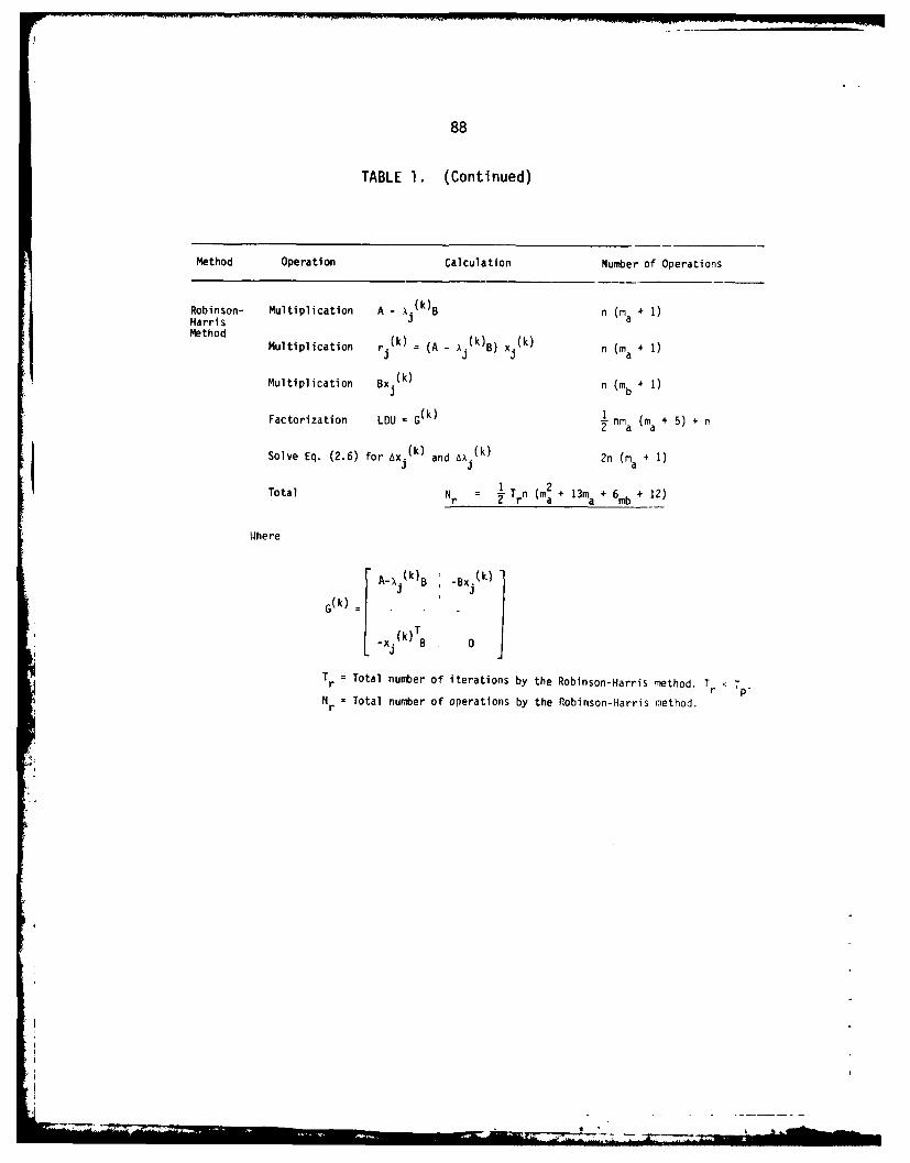
88
TABLE 1. (Continued)
Method Operation Calculation Number of Operations
Robinson- Multiplication A - x.(k) B n (m + 1)Harris 3 aMethod Multiplication r.i (k) = (A (k- ) k n (m + 1
Multiplication Bx i(k) n (m b 1
Factorization LOU = G~k) nI2T na (m a + 5) + n
Solve Eq. (2.6) for Axj.(k) and &A i(k 2n (m a+ 1)
Total Nr .1 ( 2 ++6 +12)
Where
rA-x (k)B B (k)
G ~ ~ (k T~ - .T r Total number of iterations by the Robinson-Harris method. Tr T PN r Total number of operations by the fobinson-Harris method.
r_7lot

ADOA098 786 ILLINOIS UNIV AT URBANA DEPT OF CIVIL ENGINEERING FIG 12/1
SOLUTION TECHNIQUES FOR LARGE EIGENVALUE PROBLEMS IN STRUCTURAL-ETClulJUN 79 1 LEE, A R ROBINSON NOO "?75_C0O 164
UNCLASSIFIED UILU-ENG-79-2006 NL2IIIIIEEIIIIE

1111 _1W &ILU '-ILI
MICROCOPY RESOLUTION TEST CHARTNATIONAL AUR£AU OF STANDARDS 963 A
k ii • •

Li89
TABLE 1. (Continued)
Method Operation Calculation Number of Operations
Subspace Factorizatio LU = A nmia (ma + 3)/2IterationMethod
Iteration
multiplication BX(k-1) qn (2mb + 1)
Solve for Y(k) AY(k) = BX(k-l) qn (2m + 1)
a
Multiplication A*(k) = Y (k)TBX(k-1) qn (q + 1)12
Multiplication BY(k) qn (2mb + 1)
*(k) y(k)TBy(k)
Multiplication B = qn (q + 1)12
Solve for Z(k) A*(k)z(k) = *(k)z(k)D(k) 0 (q3 neglected
and D(k )
Multiplication X(k) = Z(k)1 (k) nq2
Subtotal qn (2ma + 4mb + 2q + 4)
Sturm Sequence Check
"(k) kSMultiplication A-x pb+1
Factorization LU = A-Ap (k)B nma (ma + 3)/2
Total Ns = Tsqn (2m) +4 + 2q + 4) + n (m + 3m + mS s a) +mb a a + b+ 1)
Note: q = max (2p, p+8)
Ts = Total number of iterations by subspace iteration ethod.
Ns = Total number of ooerations by subsoace iteration method.
It is assumed that ma 1%.a-,L
IEI

IV
gO
TABLE 2. EIGENVALUES OF THE PLANE FRAME PROBLEM(DISTINCT ROOTS)
Method Eigenvaluesof Iteration
Analysis Number (1) (2) (3) (4)
Proposed 0 0.474744x100 0.443880x10
1 0.132953x10² 0.284745x10²
Method (0.36x10⁻² )* (0.28x10- 1) (0.77x10⁻¹ ) (0.22x100 )
I 0.474744x100 0.443876x101 0.132921x10² 0.284091x10²
(0.44x10⁵) (0.45x10
- 3) (0.38x10²) (0.27x10
1)
2 0.474744x100 0.443876x10
1 0.132921x10² 0.284091x10
2
(0.82x10 13) (0.27x10" ) (0.17x10- ) (0.18x10 3 )
3 0.284091x10²
(0.19x10 "5 )
4 0.284091x10²
(0.23x10 )
Robinson 0 0.474744x100 0.443880x10
1 0.132953x10² 0.284745x10
2
Harris (0.36x10⁻²) (0.28x10⁻¹) (0.77x10-) (0.22x100Method
1 0.474744x100 0.443876x10
1 0.132921x10² 0.284091x0
2
(0.44x10"5 ) (0.45x10 3 ) (0.38x10"2 ) (0.27x10- 1 )
2 0.474744x100 0.443876x10
1 0.132921x10² 0.284091x10
2
(0.82x0 13 ) (0.2740
9 ) (0.17x10 6 ) (0.18x0
- 3
3 0.284091x0 2
(0.13x0 )
* Numbers in parentheses indicate errors in the approximate
eigenvectors xj(k)
-
| oa
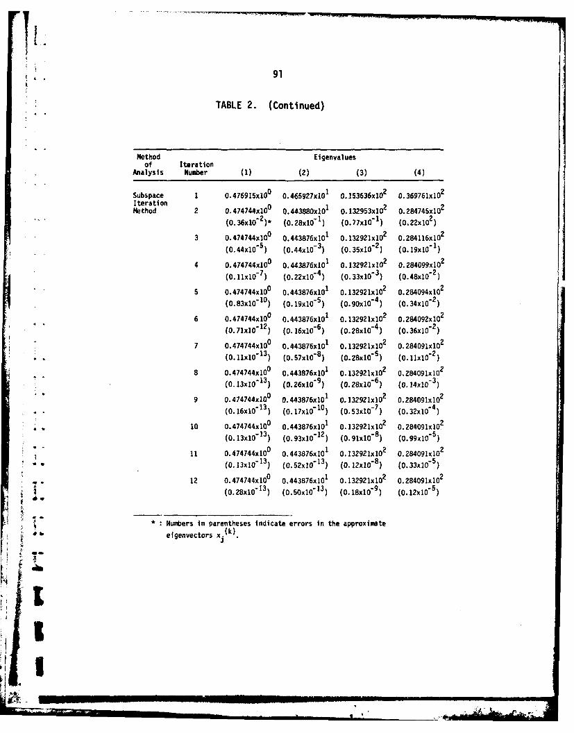
91
TABLE 2. (Continued)
Method Eigenvaluesof Iteration
Analysis Number (1) (2) (3) (4)
Subspace 1 0.476915x100 0.465927x10
1 0.153636x10² 0.369761x10
2
Iteration 0 1Method 2 0.474744x10 0.443880x10 0.132953x10² 0.284745x10²
(0.36x10 2)* (0.28x10" 1) (0.77x10" 1) (0.22x10² )
3 0.474744x100 0.443876x10' 0.132921x10
2 0.284116x10²
(0.44x10"5) (0.44x10 3 ) (0.35x10 2 ) (0.19xlO" )
4 0.474744x100 0.443876x10
1 0.132921x10² 0.284099x10
2
(0.11x10 7) (0.22x10⁻⁴ ) (0.33x10"3 ) (0.48x10 2 )
5 0.474744x100 0.443876x10
1 0.132921x10² 0.284094x10
2
(0.83x10 10 ) (0.19x10 5) (0.90x10 4 ) (0.34x10" )
6 0.474744x100 0.443876x10
1 0.132921x10² 0.284092x10
2
(0.71x10⁻¹²) (O.16xlO
-6) (0.28x10⁻⁴) (0.36x10
- 2)
7 0.474744x100 0.443876x101 0.132921x10² 0,284091x10²
(0.11x10"13) (0.57x10"8 ) (0.28x10 5 ) (0.11x10 2 )
8 0.474744x100 0.443876x10
1 0.132921x10² 0.284091x10
2
(0.13x013) (0.26xI0
-9) (0.28x10⁶) (0.14x10
" )
9 0.474744x00 0.443876x10
1 0.132921x10² 0.284091x10
2
(0.16x10³ ) (0.17x&
1 0 ) (0.53x10 - ) (0.32x10
" )
* 10 0.474744x100 0.443876x101 0.132921x10² 0.284091x10²
(0.13x10⁻¹ 3 ) (0.93x0
"12 ) (0.91x10- ) (0.99x10
" )
11 0.474744x00 0.443876x101 0.132921x10
2 0.284091x10²
(0. 13xlO 13 ) (0.52x10 13 ) (0.12xlO " ) (0.33x10- )
12 0.474744x100 0.443876x101 0.132921x10² 0.284091x10²
(0.28x10¹³) (0.50x10
13) (0.18xl9) (0.12x10
5)
• Numbers in parentheses Indicate errors in the approximate
*eigenvectors x W.
I
£

92
TABLE 3. EIGENVALUES OF THE CIRCULAR ARCH PROBLEM(DISTINCT ROOTS)
Method Eigenvalues/xo*of Iteration
Analysis Number (1) (2) (3)
Proposed 0 0.102714x10 2 0.919516x10"2 0.363073x10 1
Method 1 0.102640x10"2 0.909467x10⁻² 0.341422x10 "
(0.59x10⁻³)** (0.53x10⁻² ) (0.35x10"1 )
2 0.102640x10"2 0.909467x10 2 0.341448x10 1
(0.26x0_8) (0.10xo - ) (0.21x10_3)
3 0.909467x10 2 0.341448x10 1
(0.10x10 8) (0.17x10 "5 )
4 0.341448x10 1
(0.33x10⁷)
Robinson- 0 0.102714x10 "2 0.919516x10"2 0.363073x10 1
Harris -2Method 1 0.102640x10 0.909467x10 2 0.341422x10"
(0.59x10 ) (0.53x10 2 ) (0.35x10"1 )
2 0.102640x10 2 0.909467x10⁻² 0.341448x10 1
(0.26x10 8) (0.10x10 5 ) (0.21x10"3 )
3 0.909467x10 2 0.341448x1 "1
(0.45x10 12 ) (0.20x10 )
A 0 E/Pa2(-v
2 )"
Numbers in parentheses indicate errors in the approximate(k)
elgenvectors xj
.1J

Li 93
TABLE 3. (Continued)
Method Elgenvalues/x*of Iteration
Analysis Number (1) (2) (3)
- Subspace 1 0.102714x10"2 0.919516x10" 2 0.363073x10 1
IterationMethod 2 0.102640x10 2 0.909468x10 2 0.341476x10 1
(0.59x1O3)** (0.52x0
2) (0.32x101)
3 0.102640x10"2 0.909467x10"2 0.341448x10 1
(0.41x10⁶ ) (0.62x10 4) (0.26x10"2 )
0 .102640x10- 0.909467x10 2 0.341448x10 1
(0.58x10 9) (0.12x10 5) (0.23x0 "3)
5 0.102640x10 2 0.909467x10 2 0.341448x10 1
(0.12x10"11) (0.28x10⁷ ) (0.21x10⁴ )
6 0.102640x10 2 0.909467x10⁻² 0.341448x10 1
• . (0.23x10 13) (0.79x10 9) (0.19x10 5)
0.102640x10 2 0.909467x10 2 0.341448x10 1
(.12x10 - 3 ) (0.25x10 10 ) (0.17x10⁻⁶ )
i 2
No E/pa2(1-v2).
** Numbers in parentheses indicate errors in the approximate
eigenvectors xj (k)
iN
I"!

L.
94
TABLE 4. EIGENVALUES OF THE SQUARE PLATE PROBLEM(DOUBLE ROOTS)
Method Elgenvalues/a*of Iteration
Analysis Number (1) (2) (3) (4)
Proposed 0 0.375840x101 0.230212x10² 0.230212x10² 0.530627x10²
Method 1 0.375838x101 0.230121x10² 0.230121x10² 0.529932x10²
(0.80x10⁻³)** (0.10x10 1) (0.10x10 1) (0.21x10 ")
2 0.375838x101 0.230121x10² 0.230121x10² 0.529932x10²
(0.44x10⁻¹¹) (0.46x10 7) (0.46x10 "7) (0.59x10 6 )
Subspace 1 0.375840x101 0.230212x10² 0.230212x10² 0.530627x10²
IterationMethod 2 0.375838x101 0.230121x10² 0.230121x10² 0.529932x10²
(0.800x1 3) (0.10x10 1) (0.10x10⁻¹) (0.21x10"1)
3 0.375838x101 0.230121x10² 0.230121x10² 0.529932x10²
(0.65x10"6) (0.11x10"3) (0.11x10 3) (0.43x10"3)
4 0.375838x10 1 0.230]21x102 0.230121x10² 0.529932x10²
(0.53x10"9) (0.13x10"5) (0.13x10 5) (0.90x10 5 )
5 0.375838x101 0.230121x10² 0.230121x10² 0.529932x10 2
(0.44x10 12) (0.15x10⁻⁷) (0.15x10 7) (0.19x10 " )
* = 14De/(a4), where 0e = Eh
3/12(1 - v2)
Numbers in parentheses indicate errors in the approximate(k)elgenvectors yj
4.
[I

95
TABLE 5. EIGENVALUES OF THE RECTANGULAR PLATE PROBLEMT L 5(CLOSE ROOTS)
Method Elgenvalues/m*of Iteration
Analysis Number (1) (2) (3) (4)
Proposed 0 0.368470x10 1 0.222957x10² 0.228454x10² 0.520215x10²
Method 1 0.268468x101 0.222868x10 2 0.228264x10² 0.519522x10²
(0.80 x0 3 ) (0.100l1 ) (0.l0x 10" ) (0.21x10"1)
2 0.368468x101 0.22288x10
2 0.228364x10² 0519533x10
2
(0.44x10- 11 ) (0.47x10⁻⁷) (0.45x10
- 7) (0.59x10⁻⁶)
Subspace 1 0.368470x101 0.222957x10² 0.228454x10
2 0.520215x10²
IterationMethod 2 0.368468x10 1 0.222868x10² 0.228364x10² 0.519533x10²
(0.80x10"3 ) (0.10x10"1) (0.10x10 "1 ) (0.21x10" )3 0.368468x10
1 0.222868x10² 0.228364x10
2 0.519533x10²
(0.65x10- ) ( 3.lxlO) (0.11xlO
3) (0.43x10 )
4 0.368468x10 1 0.222868x10² 0.228364x10² 0.519533x10²(0.53x10 9) (0.13x1&O5 ) (O.13x1 5) (0.90xlO- )
5 0.368468x10' 0.222868x10² 0.228364x10² 0.519533x10²
(0.46x10¹² ) (O.15xlO
7) (0.14x0 ) (O.19x10- 6 )
= eD /(ap), where D = Eh3 /120 2- .
** Numbers in parentheses indicate errors in the approximate
I ] eigenvectors yj(k)
1,
1124.
'I
Ip,

96 .
TABLE 6. COMPARISON OF THE TOTAL NUMBER OF OPERATIONS
Input Data Nimber of Number of Operations Ratio -
Problem IterationsType n %m p q Tp Tr Ts Np Nr Ns NJNp Ns/N €
Frame 330 35 35 4 10 10 9 12 3.50x10⁶ 4.57x10⁶ 9.72x10⁶ 1.31 2.78
Arch 22 4 0 3 5 9 8 7 8.87x10 3 9.77x10³ 1.76x10⁴ 1.10 1.98
Plate 39 16 16 4 9 8 - 5 1.27x 5 - 2.20x10⁵ 1.73
Note
n Order of stiffness and mass matrices
ma Average half bandwidth of stiffness matrix
m b : Average half bandwidth of mass matrix
p Number of eigenvalues and eigenvectors sought
q Number of iteration vectors. q = max (2p, p 8)
T : Number of Iterations by the proposed method
Tr Number of iterations by the Robinson-Harris method
Ts : Number of iterations by the subspace iteration method
N : Total number of operations by the proposed method
Nr Total number of operations by the Robinson-Harris method
Ns Total number of operations by the subspace iteration method
i
"' 'b '' " ' " " [ K

97
TABLE 7. COMPARISON BETWEEN THE THEORETICAL CONVERGENCE RATESFOR EIGENVECTORS AND THE NUMERICAL RESULTS - FRAME PROBLEM
(DISTINCT ROOTS)
Method Eigenvalue Numberof Iteration
Analysis Number 1 2 3 4
Proposed 1 1.9x10⁸ 6.0x10-
7 4.4x10⁵ 6.7x10
3
Method 2 1. lxl "2
3 1.2x10²
Theory 1.3x10⁻⁸ 10x10
5 3.6x10⁴ 1.2x10
2
Subspace 2 1.2x10 3 1.6x10 2 4.5x10 2 8.6x10 2
Iteration 3 2.5x10⁻³ 5.0x10"2 9.4xi0 "2 2.5x10" 1
Method 4 7.5x10⁻³ 8.7x10 "2 2.7x10"1 7.Ix1O" 1
5 8.6x10⁻³ 8.4x10⁻² 3.1xl0
1 1.1x100
6 1.5410-3 3.6x10
2 1.0x10- 1 3.lx10 1
7 * 4.6x10 -2 1.0x10- 1 1.3xlO "1
-2 -1 -18 * 6.5x10 1.9x10 2.3x109 * 5.5x10"2 1.7x10- 1 3.lxlo'1
10 5.6x10² 1.3x10
- 1 3.3x101
11 * 1.5x10- 1 3.6x101
Theory 5.6x10³ 5.ZxIO
-2 1.6xl10 3.3x10"1
IE., I * :Errors too small for comparison because of round-off error.
I'

98
TABLE 8. COMPARISON BETWEEN THE THEORETICAL CONVERGENCE RATES FOREIGENVECTORS AND THE NUMERICAL RESULTS - SQUARE PLATE PROBLEM
(DOUBLE ROOTS)
Method Elgenvalue Numberof Iteration
Analysis Number 1 2 3 4
Proposed 1 5.5x0 9 4.6xO 6 4.6x 10"6 2.8xlO -5
Method Theory 1.0xlO"6 4.7x10"4 4.7x10"4 2.3x10" 3
Subspace 2 8.lxlO 4 1.lx1O 2 1.lx10 2 2.0x10 2
Iteration 3 8.2x0 4 1.2x0 -2 1.2x0 2 2.IxlO"2
4 8.3x0 -4 1.2xlO"2 1.2xl0"2 2.lxlO"2
Theory 1.lxlO 2 6.8x10 2 6.8X10 2 1.6x0 1 -
IIm
1

99
TABLE 9. NUMERICAL CONVERGENCE RATES FOR EIGENVECTORS -RECTANGULAR PLATE PROBLEM
(CLOSE ROOTS)
Method Eigenvalue Numberof Iteration
Analysis Number 1 2 3 4
Proposed 1 5.5x10- 9 4.7x10 6 4.5x10 6 2.8x10 5
MethodISubspe:e 2 8.Ix10 4 1.1x10 - 1.1xlO " 2.0x10 2
Iteracion - 2 -2Method 3 8.2x10⁻⁴ 1.2x10⁻² 1.2x0 2 2.1xlO
4 8.7x10 4 1.2xl0 2 1.1xlO 2 2.1x10⁻²
Theory l. lxlO2 6.8x10-
2 7.0xlO2 1.6x101 1
Ii17~
1~.
~I
KI43'

100
•i (k)T (Ii)
xj' BAj (k - 0k
-(k+I) -i BAXJ 0
-(k) (k)c T
Ck+I) Cj 0
(qk) Gjk0 j
FIG. I ESTIMATION OF ERRORS IN APPROXIMATE EIGENVECTORS

*Ii101
Q . --
I~0 at 6.1 M 61.0 M-J
For All Beams and ColumnsArea of Cross-Section A -2.787xi0-I m2
:. .Moment of Inertia of Cross-Section I = 8.631x10 - 3 m4
10I
. ,.Young's Modulus E = 2.6xO Pa
-3§KMass Density p = 1.602x10⁴ kg/ni
FIG. 2 TEN-STORY, TEN-BAY PLANE FRAME
S I "U
I

III 474:NP: 716:lab78u474-619
ONR Code 474May 1980
DISTRIBUTION LIST
for
UNCLASSIFIED TECHNICAL REPORTS
The ONR Structural Mechanics Contract Research Program
This list consists of:
Part I - Government ActivitiesPart 2 - Contractors and Other
Technical Collaborators
Notes:
Except as otherwise indicated, forward one- - copy of all Unclassified Technical Reports
to each of the addressees listed herein.
U.
Where more than one attention addressee isindicated, the individual copies of thereport should be mailed separately.
I
I

474:NP:716: lab78u474-619
Part I - Government Navy (Con't.)Administrative and Liaison Activities
Naval Research LaboratoryOffice of Naval Research Washington, D.C. 20375Department of the Navy Attn: Code 8400Arlington, Virginia 22217 8410Attn: Code 474 (2) 8430
Code 471 8440Code 200 6300
6390Director 6380Office of Naval Research
Eastern/Central Regional Office David W. Taylor Naval Ship Research666 Summer Street and Development CenterBoston, Massachusetts 02210 Annapolis, Maryland 21402
Attn: Code 2740Director 28Office of Naval Research 281
Branch Office536 South Clark Street Naval Weapons CenterChicago, Illinois 60605 China Lake, California 93555
Attn: Code 4062Director 4520I Office of Naval ResearchNew York Area Office Commanding Officer715 Broadway - 5th Floor Naval Civil Engineering LaboratoryNew York, New York 10003 Code L31
Port Hueneme, California 93041DirectorOffice of Naval Research Naval Surface Weapons Center
Western Regional Office White Oak1030 East Green Street Silver Spring, Maryland 20910Pasadena, California 91106 Attn: Code R-10
G-402Naval Research Laboratory (6) K-82Code 2627Washington, D.C. 20375 Technical Director
Naval Ocean Systems CenterDefense Technical Information Center (12) San Diego, California 92152Cameron StationAlexandria, Virginia 22314 Supervisor of Shipbuilding
U.S. NavyNavy Newport News, Virginia 23607
Undersea Explosion Research Division Navy Underwater SoundNaval Ship Research and Development Reference Division
Center Naval Research LaboratoryNorfolk Naval Shipyard P.O. Box 8337Portsmouth, Virginia 23709 Orlando, Florida 32806Attn: Dr. E. Palmer, Code 177tw
Chief of Naval operationsDepartment of the NavyWashington, D.C. 20350Attn: Code OP-098

474:NP:716 :lab78u474-619
Navy (Con't.) Navy (Con't.)
Strategic Systems Project Office Commander and DirectorDepartment of the Navy David W. Taylor Naval ShipWashington, D.C. 20376 Research and Development CenterAttn: NSP-200 Bethesda, Maryland 20084
Attn: Code 042Naval Air Systems Command 17Department of the Navy 172Washington, D.C. 20361 173Attn: Code 5302 (Aerospace and Structures) 174
604 (Technical Library) 1800320B (Structures) 1844
012.2
Naval Air Development Center 1900Warminster, Pennsylvania 18974 1901Attn: Aerospace Mechanics 1945
Code 606 1960"" 1962
U.S. Naval AcademyEngineering Department Naval Underwater Systems CenterAnnapolis, Maryland 21402 Newport, Rhode Island 02840
Attn: Bruce Sandman, Code 3634Naval Facilities Engineering Command200 Stovall Street Naval Surface Weapons CenterAlexandria, Virginia 22332 Dahlgren Laboratory
. Attn: Code 03 (Research and Development) Dahlgren, Virginia 2244804B Attn: Code G04045 G20
14114 (Technical Library)Technical Director
W' Naval Sea Syitems Command Mare Island Naval ShipyardDepartment of the Navy Vallejo, California 94592Washington, D.C. 20362Attn: Code 05H U.S. Naval Postgraduate School
312 Library322 Code 0384
323 Monterey, California 9394005R32R Webb Institute of Naval ArchitecturejI Attn: Librarian
Crescent Beach Road, Glen CoveLong Island, New York 11542
Army
Commanding Officer (2)U.S. Army Research Office
P.O. Box 12211Research Triangle Park, NC 27709Attn: Mr. J. J. Murray, CRD-AA-IP
I
474:NP:716:lab78u474-619
Amy (Con't.) Air Force (Con't.)
Watervliet Arsenal Chief, Civil Engineering BranchMAGGS Research Center WLRC, Research DivisionWatervliet, New York 12189 Air Force Weapons LaboratoryAttn: Director of Research Kirtland Air Force Base
Albuquerque, New Mexico 87117U.S. Army Materials and Mechanics
Research Center Air Force Office Of Scientific ResearchWatertown, Massachusetts 02172 Bolling Air Force BaseAttn: Dr. R. Shea, DRXMR-T Washington, D.C. 20332
Attn: Mechanics DivisionU.S. Army Missile Research and
Development Center Department of the Air ForceRedstone Scientific Information Air University Library
Center Maxwell Air Force BaseChief, Document Section Montgomery, Alabama 36112Redstone Arsenal, Alabama 35809
Other Government ActivitiesArmy Research and Development
Center CommandantFort Belvoir, Virginia 22060 Chief, Testing and Development Division
U.S. Coast GuardNASA 1300 E Street, NW.
Washington, D.C. 20226National Aeronautics and SpaceAdministration Technical Director
Structures Research Division Marine Corps DevelopmentLangley Research Center and Education CommandLangley Station Quantico, Virginia 22134Hampton, Virginia 23365
Director Defense ResearchNational Aeronautics and Space and EngineeringAdministration Technical Library
Associate Administrator for Advanced Room 3C128Research and Technology The Pentagon
Washington, D.C. 20546 Washington, D.C. 20301
Air Force Dr. M. GausNational Science Foundation
Wright-Patterson Air Force Base Environmental Research DivisionDayton, Ohio 45433 Washington, D.C. 20550Attn: AFFDL (FB)
(FBR) Library of Congress(FBE) Science and Technology Division(FBS) Washington, D.C. 20540AFL(MBM)
Director --
Chief Applied Mechanics Group Defense Nuclear AgencyU.S. Air Force Institute of Technology Washington, D.C. 20305Wright-Patterson Air Force Base Attn: SPSSDayton, Ohio 45433 Ji U

474:NP:716:lab78u474 -619
Other Government Activities (Con't) Universities (Con't)
Mr. Jerome Persh Dr. Harold Liebovitz, DeanStaff Specialist for Materials bhool of Engineering and
and Structures Applied ScienceOUSDR&E, The Pentagon George Washington UniversityRoom 3DI089 Washington, D.C. 20052Washington, D.C. 20301
Professor Eli SternbergChief, Airframe and Equipment Branch California Institute of Technology
N FS-120 Division of Engineering andOffice of Flight Standards Applied SciencesFederal Aviation Agency Pasadena, California 91109Washington, D.C. 20553
Professor Paul M. NaghdiNational Academy of Sciences University of CaliforniaNational Research Council Department of Mechanical EngineeringShip Hull Research Committee Berkeley, California 947202101 Constitution AvenueWashington, D.C. 20418 Professor A. J. DurelliAttn: Mr. A. R. Lytle Oakland University
School of EngineeringNational Science Foundation Rochester, Missouri 48063Engineering Mechanics SectionDivision of Engineering Professor F. L. DiMaggioWashington, D.C. 20550 Columbia University
Department of Civil EngineeringPicatinny Arsenal New York, New York 10027
Plastics Technical Evaluation CenterAttn: Technical Information Section Professor Norman JonesDover, New Jersey 07801 The University of Liverpool
Department of Mechanical Engineering
Maritime Administration P. 0. Box 147Office of Maritime Technology Brownlow Hill14th and Constitution Avenue, NW. Liverpool L69 3BXWashington, D.C. 20230 England
PART 2 - Contractors and Other Technical Professor E. J. Skudrzyk
Collaborators Pennsylvania State UniversityApplied Research Laboratory
Universities Department of PhysicsState College, Pennsylvania 16801
Dr. J. Tinsley OdenUniversity of Texas at Austin Professor J. Kloaner345 Engineering Science Building Polytechnic Institute of New YorkAustin, Texas 78712 Department of Mechanical and
Aerospace Engineering
Professor Julius Miklowitz 333 Jay StreetCalifornia Institute of Technology Brooklyn, New York 11201Division of Engineering
and Applied Sciences Professor R. A. SchaperyPasadena, California 91109 Texas A&M University
Department of Civil EngineeringCollege Station, Texas 77843

474:NP:716:lab
78u474-619
Universities (Con't.) Universities (Con't)
Professor Walter D. Pilkey Professor A. C. EringenUniversity of Virginia Princeton UniversityResearch Laboratories for the Department of Aerospace and
Engineering Sciences and Mechanical SciencesApplied Sciences Princeton, Nev Jersey 08540
Charlottesville, Virginia 22901Professor E. H. Lee
Professor K. D. Willmert Stanford UniversityClarkson College of Technology Division of Engineering MechanicsDepartment of Mechanical Engineering Stanford, California 94305Potsdam, New York 13676
Professor Albert I. KingDr. Walter E. Haisler Wayne State UniversityTexas A&M University Biomechanics Research CenterAerospace Engineering Department Detroit, Michigan 48202College Station, Texas 77843
Dr. V. R. HodgsonDr. Hussein A. Kamel Wayne State UniversityUniversity of Arizona School of MedicineDepartment of Aerospace and Detroit, Michigan 48202Mechanical Engineering
Tucson, Arizona 85721 Dean B. A. BoleyNorthwestern University
Dr. S. J. Fenves Department of Civil EngineeringCarnegie-Mellon University Evanston, Illinois 60201Department of Civil EngineeringSchenley Park Professor P. G. Hodge, Jr.Pittsburgh, Pennsylvania 15213 University of Minnesota
Department of Aerospace EngineeringDr. Ronald L. Huston and MechanicsDepartment of Engineering Analysis Minneapolis, Minnesota 55455University of CincinnatiCincinnati, Ohio 45221 Dr. D. C. Drucker
University of IllinoisProfessor G. C. M. Sih Dean of EngineeringLehigh University Urban&, Illinois 61801Institute of Fracture and
Solid Mechanics Professor N. M. NewmarkBethlehem, Pennsylvania 18u15 University of Illinois
Department of Civil EngineeringProfessor Albert S. Kobayashi Urbana, Illinois 61803University of WashingtonDepartment of Mechanical Engineering Professor E. ReissnerSeattle, Washington 98105 University of California, San Diego
Department of Applied MechanicsProfessor Daniel Frederick La Jolla, California 92037Virginia Polytechnic Institute and
State University Professor William A. NashDepartment of Engineering Mechanics University of MassachusettsBlacksburg, Virginia 24061 Department of Mechanics and
Aerospace EngineeringAmherst, Massachusetts 01002 [_i
II II l lli I I I l i i , ii l l

474:NP:716:lab78u474-619
* Universities (Con't) Universities (Con't)
Professor G. Herrmann Professor Joseph L. RoseStanford University Drexel UniversityDepartment of Applied Mechanics Department of Mechanical EngineeringStanford, California 94305 and Mechanics
Philadelphia, Pennsylvania 19104Professor J. D. AchenbachNorthwest University Professor B. K. DonaldsonDepartment of Civil Engineering University of Maryland
* Evanston, Illinois 60201 Aerospace Engineering DepartmentCollege Park, Maryland 20742
- - Professor S. B. DongUniversity of California Professor Joseph A. Clark
" Department of Mechanics Catholic University of AmericaLos Angeles, California 90024 Department of Mechanical Engineering
Washington, D.C. 20064: S oProfessor Burt Paul
University of Pennsylvania Dr. Samuel B. BatdorfTowns School of Civil and University of CaliforniaMechanical Engineering School of Engineering
Philadelphia, Pennsylvania 19104 and Applied ScienceI -Los Angeles, California 90024Professor H. W. Liu
low Syracuse University Professor Isaac FriedDepartment of Chemical Engineering Boston University
and Metallurgy Department of MathematicsSyracuse, New York 13210 Boston, Massachusetts 02215
Professor S. Bodner Professor E. KremplTechnion R&D Foundation Rensselaer Polytechnic InstituteHaifa, Israel Division of Engineering
Engineering MechanicsProfessor Werner Goldsmith Troy, New York 12181University of CaliforniaDepartment of Mechanical Engineering Dr. Jack R. Vinson
- Berkeley, California 94720 University of DelawareDepartment of Mechanical and Aerospace
Professor R. S. Rivlin Engineering and the Center forLehigh University Composite MaterialsCenter for the Application Newark, Delaware 19711
of Mathemat icsBethlehem, Pennsylvania 18015 Dr. J. Duffy
Brown UniversityProfessor F. A. Cozzarelli Division of EngineeringState University of New York at Providence, Rhode Island 02912
BuffaloDivision of Interdisciplinary Studies Dr. J. L. SwedlowKarr Parker Engineering Building Carnegie-Mellon UniversityChemistry Road Department of Mechanical EngineeringBuffalo, New York 14214 Pittsburgh, Pennsylvania 15213
II

474:NP:716:lab
78u474-619
Universities (Con't) Universities (Con't)
Dr. V. K. Varadan Professor V. H. NeubertOhio State University Research Foundation Pennsylvania State UniversityDepartment of Engineering Mechanics Department of Engineering ScienceColumbus, Ohio 43210 and Mechanics
University Park, Pennsylvania 16802Dr. Z. HashinUniversity of Pennsylvania Professor A. W. LeissaDepartment of Metallurgy and Ohio State UniversityMaterials Science Department of Engineering Mechanics
College of Engineering and Columbus, Ohio 43212Applied Science
Philadelphia, Pennsylvania 19104 Professor C. A. BrebbiaUniversity of California, Irvine
Dr. Jackson C. S. Yang Department of Civil EngineeringUniversity of Maryland School of EngineeringDepartment of Mechanical Engineering Irvine, California 92717College Park, Maryland 20742
Dr. George T. RahnProfessor T. Y. Chang Vanderbilt UniversityUniversity of Akron Mechanical Engineering andDepartment of Civil Engineering Materials Science
Akron, Ohio 44325 Nashville, Tennessee 37235
Professor Charles W. Bert Dean Richard H. GallagherUniversity of Oklahoma University of ArizonaSchool of Aerospace, Mechanical, College of Engineering
and Nuclear Engineering Tucson, Arizona 85721Norman, Oklahoma 73019
Professor E. F. RybickiProfessor Satya N. Atluri The University of TulsaGeorgia Institute of Technology Department of Mechanical EngineeringSchool of Engineering and Tulsa, Oklahoma 74104Mechanics
Atlanta, Georgia 30332 Dr. R. HaftkaIllinois Institute of Technology
Professor Graham F. Carey Department of Mechanics and MechanicalUniversity of Texas at Austin and Aerospace EngineeringDepartment of Aerospace Engineering Chicago, Illinois 60616
and Engineering MechanicsAustin, Texas 78712 Professor J. G. de Oliveira
Massachusetts Institute of Technology
Dr. S. S. Wang Department of Ocean EngineeringUniversity of Illinois 77 Massachusetts AvenueDepartment of Theoretical and Cambridge, Massachusetts 02139
Applied MechanicsUrbana, Illinois 61801 Dr. Bernard W. Shaffer
Polytechnic Institute of New YorkProfessor J. F. Abel Route 110
Cornell University Farmingdale, New York 11735Department of Theoretical
and Applied Mechanics
Ithaca, New York 14853
F[;

474:NP:716:lab
- 78u474-6 19
Industry and Research Institutes Industry and Research Institutes (Con't)
* , Dr. Norman Hobbs Dr. T. L. GeersKaman AviDyne Lockheed Missiles and Space Company
- Division of Kaman 3251 Hanover StreetSciences Corporation Palo Alto, California 94304
Burlington, Massachusetts 01803
Mr. William CaywoodArgonne National Laboratory Applied Physics Laboratory
* . Library Services Department Johns Hopkins Road9700 South Cass Avenue Laurel, Maryland 20810Argonne, Illinois 60440
Dr. Robert E. DunhamDr. H. C. Junger Pacifica TechnologyCambridge Acoustical Associates P.O. Box 14854 Rindge Avenue Extension Del Mar, California 92014Cambridge, Massachusetts 02140
Dr. M. F. KanninenMr. 1. H. Torrance Battelle Columbus LaboratoriesGeneral Dynamics Corporation 505 King AvenueElectric Boat Division Columbus, Ohio 43201Groton, Connecticut 06340
Dr. A. A. Hochrein- Dr. J. E. Greenspon Daedalean Associates, Inc.
J. G. Engineering Research Associates Springlake Research Road3831 Menlo Drive 15110 Frederick RoadBaltimore, Maryland 21215 Woodbine, Maryland 21797
Newport News Shipbuilding and Dr. James W. JonesDry Dock Company Swanson Service Corporation
* Library P.O. Box 5415Newport News, Virginia 23607 Huntington Beach, California 92646
* o Dr. W. F. Bozich Dr. Robert E. NickellMcDonnell Douglas Corporation Applied Science and Technology
S"5301 Bolsa Avenue 3344 North Torrey Pines CourtHuntington Beach, California 92647 Suite 220
La Jolla, California 92037- Dr. H. N. Abramson
Southwest Research Institute Dr. Kevin Thomas8500 Culebra Road Westinghouse Electric Corp.San Antonio, Texas 78284 Advanced Reactors Division
P. 0. Box 158* . . Dr. R. C. DeHart Madison, Pennsylvania 15663
Southwest Research Institute- 8500 Culebra Road Dr. H. D. Hibbitt
* San Antonio, Texas 78284 Hibbitt & Karlsson, Inc.132 George M. Cohan Boulevard
Dr. M. L. Baron Providence, Rhode Island 02903Weidlinger Associates1 110 East 59th Street Dr. R. D. MindlinNew York, New York 10022 89 Deer Hill Drive
L Ridgefield, Connecticut 06877

r ! .
474:NP: 716: lab78u474-619
industry and Research Institutes (Con't)
Dr. Richard E. DameMega Engineering11961 Tech RoadSilver Spring, Maryland 20904
Mr. G. M. StanleyLockheed Palo Alto ResearchLaboratory
3251 Hanover StreetPalo Alto, California 94304
Mr. R. L. CloudRobert L. Cloud Associates, Inc.2972 Adeline StreetBerkeley, California 94703
i[
__ __ _ _ i
