solutions chapter 2 rootfinding 2.1 bisection...
TRANSCRIPT

Bisection Method 1
Solutions
Chapter 2 Rootfinding
2.1 Bisection Method
1. Verify that each of the following equations has a root on the interval (0, 1).Next, perform the bisection method to determine p3, the third approximationto the location of the root, and to determine (a4, b4), the next enclosing interval.
(a) ln(1 + x) − cos x = 0 (b) x5 + 2x − 1 = 0(c) e−x − x = 0 (d) cos x − x = 0
(a) Let f(x) = ln(1 + x) − cos x. Because f is continuous on [0, 1] with f(0) =ln 1 − cos 1 = − cos 1 < 0 and f(1) = ln 2 − cos 2 ≈ 1.109 > 0, the Inter-mediate Value Theorem guarantees that there exists a p ∈ (0, 1) such thatf(p) = 0. To start the bisection method, take (a1, b1) = (0, 1). The midpointof this first interval, and our first approximation to the location of the root, is
p1 =a1 + b1
2=
0 + 1
2= 0.5.
Note that f(p1) ≈ −0.472 < 0. Since f(a1) and f(p1) are of the same sign,the Intermediate Value Theorem tells us that the root lies between p1 and b1.With (a2, b2) = (p1, b1) = (0.5, 1), our second approximation to the locationof the root is
p2 =a2 + b2
2=
0.5 + 1
2= 0.75.
Now f(0.75) ≈ −0.172 < 0, which is of the same sign as f(a2). Hence, theIntermediate Value Theorem guarantees that the root is between p2 and b2,so we take (a3, b3) = (p2, b2) = (0.75, 1). For the third iteration, we calculate
p3 =a3 + b3
2=
0.75 + 1
2= 0.875
and f(p3) ≈ −0.0124 < 0. Here, f(a3) and f(p3) are of the same sign,which implies that the root lies between p3 and b3. Finally, we set (a4, b4) =(0.875, 1).
Full file at http://AplusTestbank.eu/Solution-Manual-for-A-Friendly-Introduction-to-Numerical-Analysis-Chapters-1-2-3-5-6-130130540
2 Section 2.1
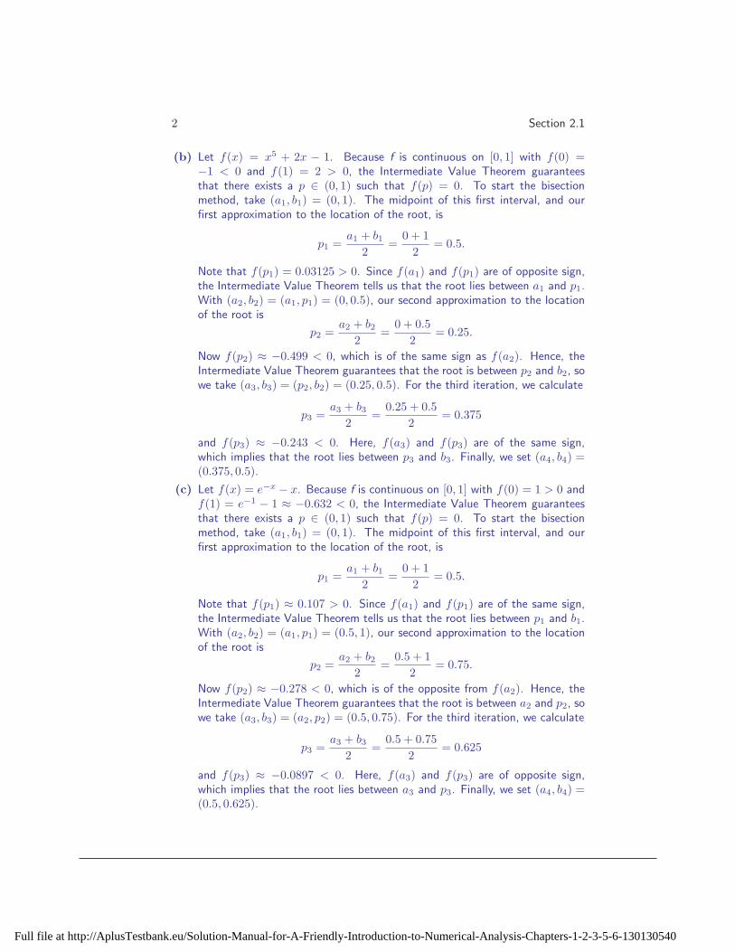
(b) Let f(x) = x5 + 2x − 1. Because f is continuous on [0, 1] with f(0) =−1 < 0 and f(1) = 2 > 0, the Intermediate Value Theorem guaranteesthat there exists a p ∈ (0, 1) such that f(p) = 0. To start the bisectionmethod, take (a1, b1) = (0, 1). The midpoint of this first interval, and ourfirst approximation to the location of the root, is
p1 =a1 + b1
2=
0 + 1
2= 0.5.
Note that f(p1) = 0.03125 > 0. Since f(a1) and f(p1) are of opposite sign,the Intermediate Value Theorem tells us that the root lies between a1 and p1.With (a2, b2) = (a1, p1) = (0, 0.5), our second approximation to the locationof the root is
p2 =a2 + b2
2=
0 + 0.5
2= 0.25.
Now f(p2) ≈ −0.499 < 0, which is of the same sign as f(a2). Hence, theIntermediate Value Theorem guarantees that the root is between p2 and b2, sowe take (a3, b3) = (p2, b2) = (0.25, 0.5). For the third iteration, we calculate
p3 =a3 + b3
2=
0.25 + 0.5
2= 0.375
and f(p3) ≈ −0.243 < 0. Here, f(a3) and f(p3) are of the same sign,which implies that the root lies between p3 and b3. Finally, we set (a4, b4) =(0.375, 0.5).
(c) Let f(x) = e−x − x. Because f is continuous on [0, 1] with f(0) = 1 > 0 andf(1) = e−1 − 1 ≈ −0.632 < 0, the Intermediate Value Theorem guaranteesthat there exists a p ∈ (0, 1) such that f(p) = 0. To start the bisectionmethod, take (a1, b1) = (0, 1). The midpoint of this first interval, and ourfirst approximation to the location of the root, is
p1 =a1 + b1
2=
0 + 1
2= 0.5.
Note that f(p1) ≈ 0.107 > 0. Since f(a1) and f(p1) are of the same sign,the Intermediate Value Theorem tells us that the root lies between p1 and b1.With (a2, b2) = (a1, p1) = (0.5, 1), our second approximation to the locationof the root is
p2 =a2 + b2
2=
0.5 + 1
2= 0.75.
Now f(p2) ≈ −0.278 < 0, which is of the opposite from f(a2). Hence, theIntermediate Value Theorem guarantees that the root is between a2 and p2, sowe take (a3, b3) = (a2, p2) = (0.5, 0.75). For the third iteration, we calculate
p3 =a3 + b3
2=
0.5 + 0.75
2= 0.625
and f(p3) ≈ −0.0897 < 0. Here, f(a3) and f(p3) are of opposite sign,which implies that the root lies between a3 and p3. Finally, we set (a4, b4) =(0.5, 0.625).
Full file at http://AplusTestbank.eu/Solution-Manual-for-A-Friendly-Introduction-to-Numerical-Analysis-Chapters-1-2-3-5-6-130130540
Bisection Method 3
(d) Let f(x) = cos x−x. Because f is continuous on [0, 1] with f(0) = 1 > 0 andf(1) = cos 1 − 1 ≈ −0.460 < 0, the Intermediate Value Theorem guaranteesthat there exists a p ∈ (0, 1) such that f(p) = 0. To start the bisectionmethod, take (a1, b1) = (0, 1). The midpoint of this first interval, and ourfirst approximation to the location of the root, is
p1 =a1 + b1
2=
0 + 1
2= 0.5.
Note that f(p1) ≈ 0.378 > 0. Since f(a1) and f(p1) are of the same sign,the Intermediate Value Theorem tells us that the root lies between p1 and b1.With (a2, b2) = (a1, p1) = (0.5, 1), our second approximation to the locationof the root is
p2 =a2 + b2
2=
0.5 + 1
2= 0.75.
Now f(p2) ≈ −0.0183 < 0, which is of the opposite from f(a2). Hence, theIntermediate Value Theorem guarantees that the root is between a2 and p2, sowe take (a3, b3) = (a2, p2) = (0.5, 0.75). For the third iteration, we calculate
p3 =a3 + b3
2=
0.5 + 0.75
2= 0.625
and f(p3) ≈ 0.186 > 0. Here, f(a3) and f(p3) are of the same sign, whichimplies that the root lies between p3 and b3. Finally, we set (a4, b4) =(0.625, 0.75).
In Exercises 2 - 5, verify that the given function has a zero on the indicatedinterval. Next, perform the first five (5) iterations of the bisection methodand verify that each approximation satisfies the theoretical error bound of thebisection method, but that the actual errors do not steadily decrease. The exactlocation of the zero is indicated by the value of p.
2. f(x) = x3 + x2 − 3x − 3, (1, 2), p =√
3
Let f(x) = x3 +x2−3x−3. Because f is continuous on (1, 2) with f(1) = −4 < 0and f(2) = 3 > 0, the Intermediate Value Theorem guarantees that there existsa p ∈ (1, 2) such that f(p) = 0. The following table summarizes the first fiveiterations of the bisection method starting from the interval (a1, b1) = (1, 2).
n pn |pn − p| (b − a)/2n
1 1.50000 0.23205 0.500002 1.75000 0.01794 0.250003 1.62500 0.10705 0.125004 1.68750 0.04455 0.062505 1.71875 0.01330 0.03125
Full file at http://AplusTestbank.eu/Solution-Manual-for-A-Friendly-Introduction-to-Numerical-Analysis-Chapters-1-2-3-5-6-130130540

4 Section 2.1
3. f(x) = sinx, (3, 4), p = π
Let f(x) = sinx. Because f is continuous on (3, 4) with f(3) = sin 3 ≈ 0.141 > 0and f(4) = sin 4 ≈ −0.757 < 0, the Intermediate Value Theorem guarantees thatthere exists a p ∈ (3, 4) such that f(p) = 0. The following table summarizes the firstfive iterations of the bisection method starting from the interval (a1, b1) = (3, 4).
n pn |pn − p| (b − a)/2n
1 3.50000 0.35841 0.500002 3.25000 0.10841 0.250003 3.12500 0.01659 0.125004 3.18750 0.04591 0.062505 3.15625 0.01466 0.03125
4. f(x) = 1 − lnx, (2, 3), p = e
Let f(x) = 1 − lnx. Because f is continuous on (2, 3) with f(2) = 1 − ln 2 ≈0.307 > 0 and f(3) = 1 − ln 3 ≈ −0.0986 < 0, the Intermediate Value Theoremguarantees that there exists a p ∈ (2, 3) such that f(p) = 0. The following tablesummarizes the first five iterations of the bisection method starting from the interval(a1, b1) = (2, 3).
n pn |pn − p| (b − a)/2n
1 2.50000 0.21828 0.500002 2.75000 0.03172 0.250003 2.62500 0.09328 0.125004 2.68750 0.03078 0.062505 2.71875 0.00047 0.03125
5. f(x) = x6 − 3, (1, 2), p = 6√
3
Let f(x) = x6 − 3. Because f is continuous on (1, 2) with f(1) = −2 < 0 andf(2) = 63 > 0, the Intermediate Value Theorem guarantees that there exists ap ∈ (1, 2) such that f(p) = 0. The following table summarizes the first fiveiterations of the bisection method starting from the interval (a1, b1) = (1, 2).
n pn |pn − p| (b − a)/2n
1 1.50000 0.29906 0.500002 1.25000 0.04906 0.250003 1.12500 0.07594 0.125004 1.18750 0.01344 0.062505 1.21875 0.01781 0.03125
6. Determine a formula which relates the number of iterations, n, required by thebisection method to converge to within an absolute error tolerance of ǫ, startingfrom the initial interval (a, b).
Full file at http://AplusTestbank.eu/Solution-Manual-for-A-Friendly-Introduction-to-Numerical-Analysis-Chapters-1-2-3-5-6-130130540

Bisection Method 5
Let p denote the location of the true root, and let pn denote the approximatelocation of the root produced by the nth iteration of the bisection method. Fromthe proof of the bisection method convergence theorem, we know that
|pn − p| ≤ b − a
2n.
The bisection method sequence will therefore converge to within an absolute toler-ance of ǫ provided
b − a
2n< ǫ.
Solving this last expression for n gives
n > log2
b − a
ǫ.
7. Modify the algorithm for the bisection method as follows. Remove the inputNmax, and calculate the number of iterations needed to achieve the specifiedconvergence tolerance using the results of Exercise 6.
Here is the modified bisection method algorithm:
GIVEN: function whose zero is to be located, f
left endpoint of interval, a
right endpoint of interval, b
convergence tolerance, ǫ
STEP 1: set Nmax = 1 + int(log2((b − a)/ǫ))STEP 2: save sfa = sign(f(a))STEP 3: for i from 1 to Nmax
STEP 4: p = a + (b − a)/2STEP 5: save sfp = sign(f(p))STEP 6: if (sfa ∗ sfp < 0) then
assign the value of p to b
elseassign the value of p to a
assign the value of sfp to sfa
endend
OUTPUT: p
8. Suppose that an equation is known to have a root on the interval (0, 1). Howmany iterations of the bisection method are needed to achieve full machineprecision in the approximation to the location of the root assuming calculationsare performed in IEEE standard double precision? What if the root were known
Full file at http://AplusTestbank.eu/Solution-Manual-for-A-Friendly-Introduction-to-Numerical-Analysis-Chapters-1-2-3-5-6-130130540
6 Section 2.1
to be contained in the interval (8,9)? (Hint: Consider the number of base 2digits already known in the location of the root and how many base 2 digits areavailable in the indicated floating point system.)
Recall that IEEE standard double precision has 53 binary digits of precision. If theroot is known to lie on the interval (0, 1), then no binary digits in the location ofthe root are known from the outset. Each iteration of the bisection method addsone binary digit to the approximation, so a total of 53 iterations will be needed toapproximate the root to full machine precision. If, on the other hand, the root isknown to lie on the interval (8, 9), then four binary digits (1000) are known fromthe outset. 49 iterations of the bisection method will be needed to approximate thelocation of the root to full machine precision.
9. By construction, the endpoints of the enclosing intervals produced by the bi-section method satisfy a1 ≤ a2 ≤ a3 ≤ · · · ≤ b3 ≤ b2 ≤ b1. Prove that thesequences {an} and {bn} converge and that
limn→∞
an = limn→∞
bn = limn→∞
pn = p.
The sequence {an} is increasing (an+1 ≥ an for all n) and bounded from above(an ≤ b1 for all n); hence, the sequence must converge. Similarly, the sequence{bn} is decreasing (bn+1 ≤ bn for all n) and bounded from below (bn ≥ a1 for alln); hence, this sequence must also converge. Now, for all n,
an ≤ pn ≤ bn,
solim
n→∞
an ≤ limn→∞
pn ≤ limn→∞
bn. (1)
From the proof of the bisection method convergence theorem, we know that
bn − an =b − a
2n,
which implies that
limn→∞
(bn − an) = 0 or limn→∞
an = limn→∞
bn. (2)
Combining (1) and (2) yields
limn→∞
an = limn→∞
bn = limn→∞
pn = p.
10. It was noted that the function f(x) = x3+2x2−3x−1 has a zero on the interval(−3,−2) and another on the interval (−1, 0). Approximate both of these zeroesto within an absolute tolerance of 5× 10⁻⁵.
Full file at http://AplusTestbank.eu/Solution-Manual-for-A-Friendly-Introduction-to-Numerical-Analysis-Chapters-1-2-3-5-6-130130540

Bisection Method 7
The following table displays the results produced by the bisection method whenapplied to the function f(x) = x3 + 2x2 − 3x − 1 with the starting intervals(a1, b1) = (−3,−2) and (a1, b1) = (−1, 0). In each case, a convergence toleranceof ǫ = 5 × 10⁻⁵ is used.
n (a1, b1) = (−3,−2) (a1, b1) = (−1, 0)1 −2.5000000000 −0.50000000002 −2.7500000000 −0.25000000003 −2.8750000000 −0.37500000004 −2.9375000000 −0.31250000005 −2.9062500000 −0.28125000006 −2.9218750000 −0.29687500007 −2.9140625000 −0.28906250008 −2.9101562500 −0.28515625009 −2.9121093750 −0.287109375010 −2.9130859375 −0.286132812511 −2.9125976562 −0.286621093812 −2.9123535156 −0.286376953113 −2.9122314453 −0.286499023414 −2.9121704102 −0.286437988315 −2.9122009277 −0.2864685059
We therefore estimate that f has roots at approximately x = −2.91220 and x =−0.28647. Both approximations are in error by at most 5 × 10⁻⁵.
11. Approximate 3√
13 to three decimal places by applying the bisection method tothe equation x3 − 13 = 0.
Let f(x) = x3 − 13. Since f(2) = −5 < 0 and f(3) = 14 > 0, we know there is aroot on the interval (a1, b1) = (2, 3). Using a convergence tolerance of ǫ = 5×10⁻⁴,the bisection method yields
n Enclosing Interval Approximation1 (2.000000,3.000000) 2.50000000002 (2.000000,2.500000) 2.25000000003 (2.250000,2.500000) 2.37500000004 (2.250000,2.375000) 2.31250000005 (2.312500,2.375000) 2.34375000006 (2.343750,2.375000) 2.35937500007 (2.343750,2.359375) 2.35156250008 (2.343750,2.351562) 2.34765625009 (2.347656,2.351562) 2.349609375010 (2.349609,2.351562) 2.350585937511 (2.350586,2.351562) 2.3510742188
Thus, 3√
13 ≈ 2.35107, with an error of at most 5 × 10⁻⁵.
12. Approximate 1/37 to five decimal places by applying the bisection method to
Full file at http://AplusTestbank.eu/Solution-Manual-for-A-Friendly-Introduction-to-Numerical-Analysis-Chapters-1-2-3-5-6-130130540
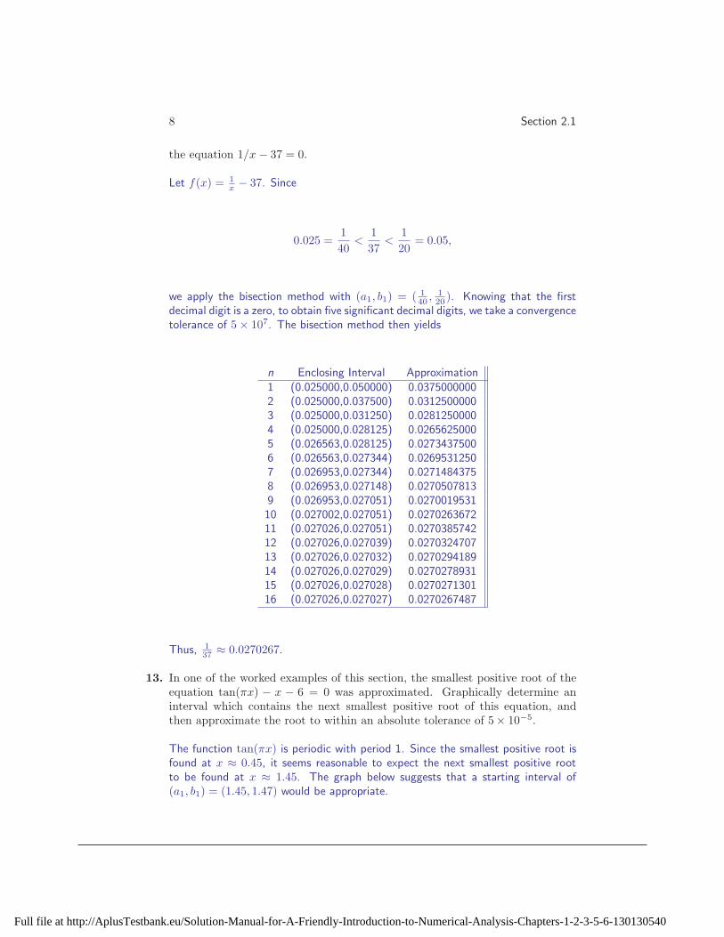
8 Section 2.1
the equation 1/x − 37 = 0.
Let f(x) = 1
x− 37. Since
0.025 =1
40<
1
37<
1
20= 0.05,
we apply the bisection method with (a1, b1) = ( 1
40, 1
20). Knowing that the first
decimal digit is a zero, to obtain five significant decimal digits, we take a convergencetolerance of 5 × 10⁷. The bisection method then yields
n Enclosing Interval Approximation1 (0.025000,0.050000) 0.03750000002 (0.025000,0.037500) 0.03125000003 (0.025000,0.031250) 0.02812500004 (0.025000,0.028125) 0.02656250005 (0.026563,0.028125) 0.02734375006 (0.026563,0.027344) 0.02695312507 (0.026953,0.027344) 0.02714843758 (0.026953,0.027148) 0.02705078139 (0.026953,0.027051) 0.027001953110 (0.027002,0.027051) 0.027026367211 (0.027026,0.027051) 0.027038574212 (0.027026,0.027039) 0.027032470713 (0.027026,0.027032) 0.027029418914 (0.027026,0.027029) 0.027027893115 (0.027026,0.027028) 0.027027130116 (0.027026,0.027027) 0.0270267487
Thus, 1
37≈ 0.0270267.
13. In one of the worked examples of this section, the smallest positive root of theequation tan(πx) − x − 6 = 0 was approximated. Graphically determine aninterval which contains the next smallest positive root of this equation, andthen approximate the root to within an absolute tolerance of 5× 10⁻⁵.
The function tan(πx) is periodic with period 1. Since the smallest positive root isfound at x ≈ 0.45, it seems reasonable to expect the next smallest positive rootto be found at x ≈ 1.45. The graph below suggests that a starting interval of(a1, b1) = (1.45, 1.47) would be appropriate.
Full file at http://AplusTestbank.eu/Solution-Manual-for-A-Friendly-Introduction-to-Numerical-Analysis-Chapters-1-2-3-5-6-130130540

Bisection Method 9
With (a1, b1) = (1.45, 1.47) and ǫ = 5 × 10⁻⁵, the bisection method yields
n Enclosing Interval Approximation1 (1.450000,1.470000) 1.46000000002 (1.450000,1.460000) 1.45500000003 (1.455000,1.460000) 1.45750000004 (1.457500,1.460000) 1.45875000005 (1.457500,1.458750) 1.45812500006 (1.457500,1.458125) 1.45781250007 (1.457500,1.457812) 1.45765625008 (1.457500,1.457656) 1.45757812509 (1.457500,1.457578) 1.4575390625
Thus, the second smallest positive root of the equation tan(πx) − x − 6 = 0 isapproximately x = 1.457539.
14. The equation (x − 0.5)(x + 1)3(x − 2) = 0 clearly has roots at x = −1, x =0.5, and x = 2. Each of the intervals listed below encompasses all of theseroots. Determine to which root the bisection method converges when each ofthe intervals below is used as the starting interval.
(a) (−3, 3) (b) (−1.5, 3) (c) (−2, 4)(d) (−2, 3) (e) (−1.5, 2.2) (f) (−7, 3)
(a) With (a1, b1) = (−3, 3), the bisection method converges toward x = −1.
(b) With (a1, b1) = (−1.5, 3), the bisection method converges toward x = 2.
(c) With (a1, b1) = (−2, 4), the bisection method converges toward x = 2.
(d) With (a1, b1) = (−2, 3), the bisection method converges toward x = 0.5.
(e) With (a1, b1) = (−1.5, 2.2), the bisection method converges toward x = −1.
(f) With (a1, b1) = (−7, 3), the bisection method converges toward x = 0.5.
Full file at http://AplusTestbank.eu/Solution-Manual-for-A-Friendly-Introduction-to-Numerical-Analysis-Chapters-1-2-3-5-6-130130540

10 Section 2.1
15. It can be shown that the equation
3
2x − 6 − 1
2sin(2x) = 0
has a unique real root.
(a) Find an interval on which this unique real root is guaranteed to exist.
(b) Using the interval found in part (a) and the bisection method, approximatethe root to within an absolute tolerance of 10−5.
(a) The equation3
2x − 6 − 1
2sin(2x) = 0
is equivalent to3
2x − 6 =
1
2sin(2x).
Because
−1
2≤ 1
2sin(2x) ≤ 1
2,
the root we are seeking must satisfy
−1
2≤ 3
2x − 6 ≤ 1
2or
11
3≤ x ≤ 13
3.
(b) With (a1, b1) = (11
3, 13
3) and a convergence tolerance of ǫ = 10−5, the bisec-
tion method yields
n Enclosing Interval Approximation1 (3.666667,4.333333) 4.00000000002 (4.000000,4.333333) 4.16666666673 (4.166667,4.333333) 4.25000000004 (4.250000,4.333333) 4.29166666675 (4.250000,4.291667) 4.27083333336 (4.250000,4.270833) 4.26041666677 (4.260417,4.270833) 4.26562500008 (4.260417,4.265625) 4.26302083339 (4.260417,4.263021) 4.261718750010 (4.260417,4.261719) 4.261067708311 (4.261068,4.261719) 4.261393229212 (4.261393,4.261719) 4.261555989613 (4.261393,4.261556) 4.261474609414 (4.261475,4.261556) 4.261515299515 (4.261475,4.261515) 4.261494954416 (4.261475,4.261495) 4.261484781917 (4.261475,4.261485) 4.2614796956
Full file at http://AplusTestbank.eu/Solution-Manual-for-A-Friendly-Introduction-to-Numerical-Analysis-Chapters-1-2-3-5-6-130130540

Bisection Method 11
Thus, the unique root of the equation
3
2x − 6 − 1
2sin(2x) = 0
is approximately x = 4.261482.
16. For each of the functions given below, use the bisection method to approximateall real zeros. Use an absolute tolerance of 10−6 as a stopping criterion.
(a) f(x) = ex + x2 − x − 4
(b) f(x) = x3 − x2 − 10x + 7
(c) f(x) = 1.05 − 1.04x + lnx
(a) Let f(x) = ex +x2 −x− 4. Observe that the equation ex +x2 −x− 4 = 0 isequivalent to the equation ex = −x2 + x + 4. The figure below displays thegraphs of y = ex and y = −x2 + x + 4.
The graphs appear to intersect over the intervals (−2,−1) and (1, 2). Usingeach of these intervals and a convergence tolerance of 10−6, the bisectionmethod yields
Full file at http://AplusTestbank.eu/Solution-Manual-for-A-Friendly-Introduction-to-Numerical-Analysis-Chapters-1-2-3-5-6-130130540
12 Section 2.1
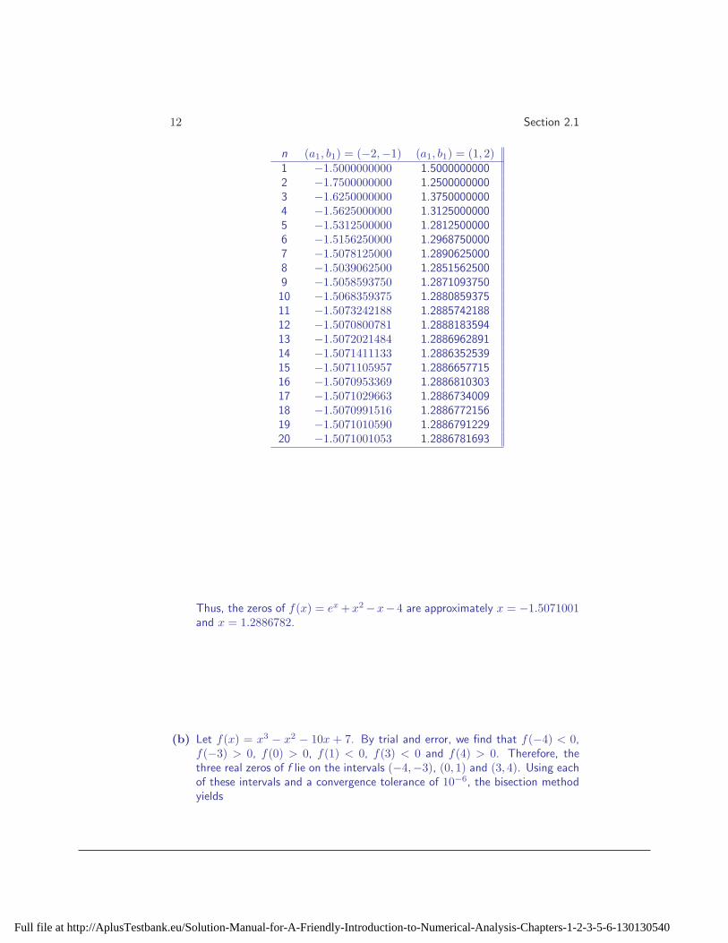
n (a1, b1) = (−2,−1) (a1, b1) = (1, 2)1 −1.5000000000 1.50000000002 −1.7500000000 1.25000000003 −1.6250000000 1.37500000004 −1.5625000000 1.31250000005 −1.5312500000 1.28125000006 −1.5156250000 1.29687500007 −1.5078125000 1.28906250008 −1.5039062500 1.28515625009 −1.5058593750 1.287109375010 −1.5068359375 1.288085937511 −1.5073242188 1.288574218812 −1.5070800781 1.288818359413 −1.5072021484 1.288696289114 −1.5071411133 1.288635253915 −1.5071105957 1.288665771516 −1.5070953369 1.288681030317 −1.5071029663 1.288673400918 −1.5070991516 1.288677215619 −1.5071010590 1.288679122920 −1.5071001053 1.2886781693
Thus, the zeros of f(x) = ex +x2 −x− 4 are approximately x = −1.5071001and x = 1.2886782.
(b) Let f(x) = x3 − x2 − 10x + 7. By trial and error, we find that f(−4) < 0,f(−3) > 0, f(0) > 0, f(1) < 0, f(3) < 0 and f(4) > 0. Therefore, thethree real zeros of f lie on the intervals (−4,−3), (0, 1) and (3, 4). Using eachof these intervals and a convergence tolerance of 10−6, the bisection methodyields
Full file at http://AplusTestbank.eu/Solution-Manual-for-A-Friendly-Introduction-to-Numerical-Analysis-Chapters-1-2-3-5-6-130130540

Bisection Method 13
n (a1, b1) = (−4,−3) (a1, b1) = (0, 1) (a1, b1) = (3, 4)1 −3.5000000000 0.5000000000 3.50000000002 −3.2500000000 0.7500000000 3.25000000003 −3.1250000000 0.6250000000 3.37500000004 −3.0625000000 0.6875000000 3.31250000005 −3.0312500000 0.6562500000 3.34375000006 −3.0468750000 0.6718750000 3.35937500007 −3.0390625000 0.6796875000 3.35156250008 −3.0429687500 0.6835937500 3.35546875009 −3.0410156250 0.6855468750 3.357421875010 −3.0419921875 0.6845703125 3.358398437511 −3.0424804688 0.6850585938 3.357910156212 −3.0427246094 0.6853027344 3.357666015613 −3.0426025391 0.6851806641 3.357543945314 −3.0426635742 0.6852416992 3.357482910215 −3.0426940918 0.6852111816 3.357452392616 −3.0426788330 0.6852264404 3.357467651417 −3.0426864624 0.6852188110 3.357460022018 −3.0426826477 0.6852226257 3.357463836719 −3.0426845551 0.6852207184 3.357461929320 −3.0426836014 0.6852197647 3.3574628830
Thus, the zeros of f(x) = x3−x2−10x+7 are approximately x = −3.0426836,x = 0.6852198 and x = 3.3574629.
(c) Let f(x) = 1.05−1.04x+ln x. Observe that the equation 1.05−1.04x+ln x =0 is equivalent to the equation lnx = 1.04x− 1.05. The figure below displaysthe graphs of y = lnx and y = 1.04x − 1.05.
The graphs appear to intersect over the intervals (0.80, 0.85) and (1.10, 1.15).Using each of these intervals and a convergence tolerance of 10−6, the bisectionmethod yields
Full file at http://AplusTestbank.eu/Solution-Manual-for-A-Friendly-Introduction-to-Numerical-Analysis-Chapters-1-2-3-5-6-130130540
14 Section 2.1
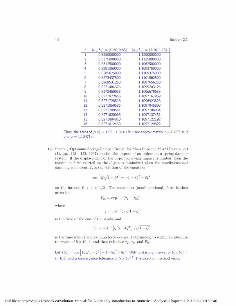
n (a1, b1) = (0.80, 0.85) (a1, b1) = (1.10, 1.15)1 0.8250000000 1.12500000002 0.8375000000 1.11250000003 0.8312500000 1.10625000004 0.8281250000 1.10937500005 0.8265625000 1.11093750006 0.8273437500 1.11015625007 0.8269531250 1.10976562508 0.8271484375 1.10957031259 0.8272460938 1.109667968810 0.8271972656 1.109716796911 0.8271728516 1.109692382812 0.8271850586 1.109704589813 0.8271789551 1.109710693414 0.8271820068 1.109713745115 0.8271804810 1.109712219216 0.8271812439 1.1097129822
Thus, the zeros of f(x) = 1.05−1.04x+ln x are approximately x = 0.8271812and x = 1.1097130.
17. Peters (“Optimum Spring-Damper Design for Mass Impact,” SIAM Review, 39(1), pp. 118 - 122, 1997) models the impact of an object on a spring-dampersystem. If the displacement of the object following impact is limited, then themaximum force exerted on the object is minimized when the nondimensionaldamping coefficient, ζ, is the solution of the equation
cos[
4ζ√
1 − ζ2
]
= −1 + 8ζ2 − 8ζ4
on the interval 0 < ζ < 1/2. The maximum (nondimensional) force is thengiven by
Fm = exp [−ζ(τf + τm)] ,
where
τf = cos−1 ζ/√
1 − ζ2
is the time of the end of the stroke and
τm = cos−1[
ζ(3 − 4ζ2)]
/√
1 − ζ2
is the time when the maximum force occurs. Determine ζ to within an absolutetolerance of 5 × 10⁻⁷, and then calculate τf , τm and Fm.
Let f(ζ) = cos[
4ζ√
1 − ζ2
]
+1−8ζ2 +8ζ4. With a starting interval of (a1, b1) =
(0, 0.5) and a convergence tolerance of 5 × 10⁻⁷, the bisection method yields
Full file at http://AplusTestbank.eu/Solution-Manual-for-A-Friendly-Introduction-to-Numerical-Analysis-Chapters-1-2-3-5-6-130130540

Bisection Method 15
n Enclosing Interval Approximation1 (0.000000,0.500000) 0.25000000002 (0.250000,0.500000) 0.37500000003 (0.375000,0.500000) 0.43750000004 (0.375000,0.437500) 0.40625000005 (0.375000,0.406250) 0.39062500006 (0.390625,0.406250) 0.39843750007 (0.398438,0.406250) 0.40234375008 (0.402344,0.406250) 0.40429687509 (0.402344,0.404297) 0.403320312510 (0.403320,0.404297) 0.403808593811 (0.403809,0.404297) 0.404052734412 (0.403809,0.404053) 0.403930664113 (0.403931,0.404053) 0.403991699214 (0.403931,0.403992) 0.403961181615 (0.403961,0.403992) 0.403976440416 (0.403961,0.403976) 0.403968811017 (0.403969,0.403976) 0.403972625718 (0.403973,0.403976) 0.403974533119 (0.403973,0.403975) 0.403973579420 (0.403973,0.403974) 0.4039731026
Thus, ζ = 0.4039731. We then calculate τf = 1.2625461, τm = 0.3533436, andFm = 0.5205986.
18. DeSantis, Gironi and Marelli (“Vector-liquid equilibrium from a hard-sphereequation of state,” Industrial and Engineering Chemistry Fundamentals, 15,182-189, 1976) derive a relationship for the compressibility factor of real gasesof the form
z =1 + y + y2 − y3
(1 − y)3,
where y is related to the van der Waals volume correction factor. If z = 0.892,what is the value of y?
Let
f(y) =1 + y + y2 − y3
(1 − y)3− 0.892.
By trial and error, we find
f(1.8) ≈ −1.298 < 0 and f(2) = 0.108 > 0.
Applying the bisection method with (a1, b1) = (1.8, 2) and a convergence toleranceof 5 × 10⁻⁵ yields
Full file at http://AplusTestbank.eu/Solution-Manual-for-A-Friendly-Introduction-to-Numerical-Analysis-Chapters-1-2-3-5-6-130130540
16 Section 2.1
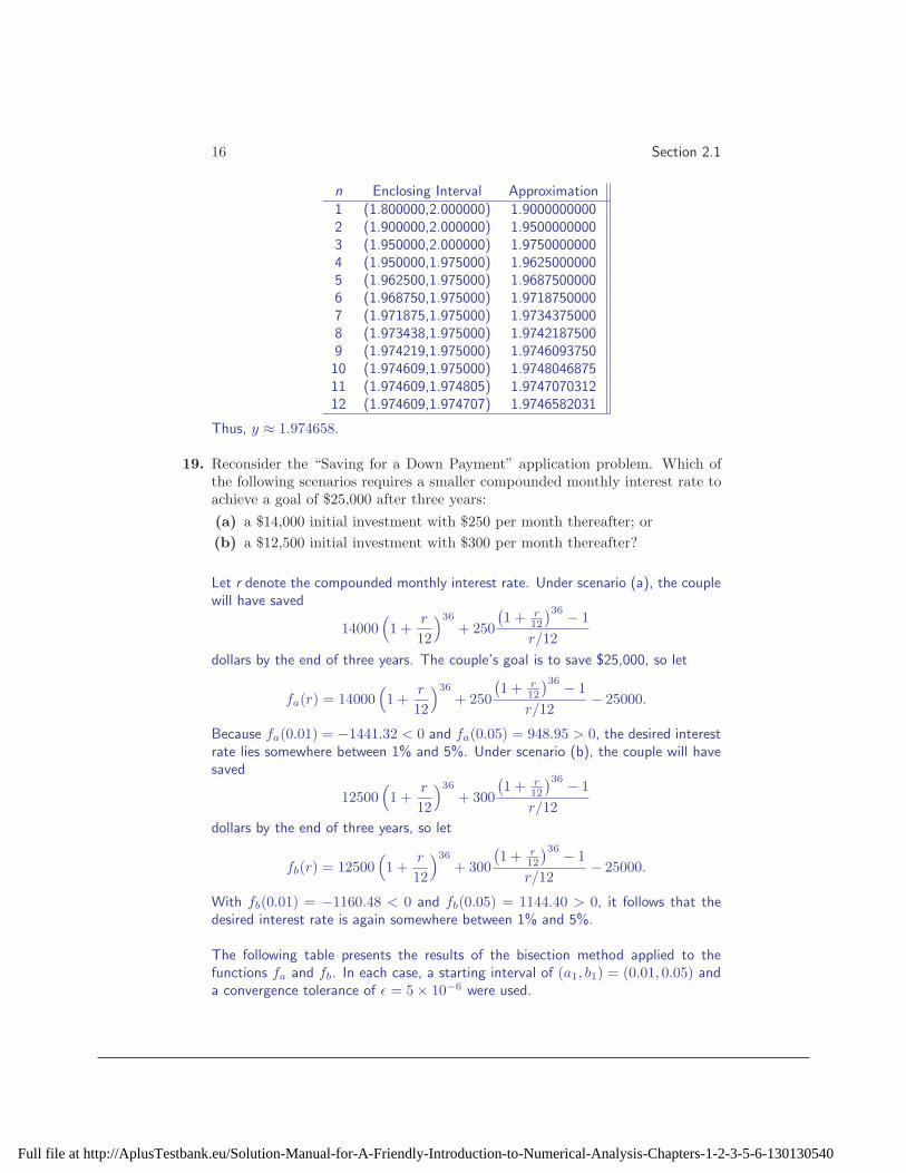
n Enclosing Interval Approximation1 (1.800000,2.000000) 1.90000000002 (1.900000,2.000000) 1.95000000003 (1.950000,2.000000) 1.97500000004 (1.950000,1.975000) 1.96250000005 (1.962500,1.975000) 1.96875000006 (1.968750,1.975000) 1.97187500007 (1.971875,1.975000) 1.97343750008 (1.973438,1.975000) 1.97421875009 (1.974219,1.975000) 1.974609375010 (1.974609,1.975000) 1.974804687511 (1.974609,1.974805) 1.974707031212 (1.974609,1.974707) 1.9746582031
Thus, y ≈ 1.974658.
19. Reconsider the “Saving for a Down Payment” application problem. Which ofthe following scenarios requires a smaller compounded monthly interest rate toachieve a goal of $25,000 after three years:
(a) a $14,000 initial investment with $250 per month thereafter; or
(b) a $12,500 initial investment with $300 per month thereafter?
Let r denote the compounded monthly interest rate. Under scenario (a), the couplewill have saved
14000(
1 +r
12
)36
+ 250
(
1 + r12
)36 − 1
r/12
dollars by the end of three years. The couple’s goal is to save $25,000, so let
fa(r) = 14000(
1 +r
12
)36
+ 250
(
1 + r12
)36 − 1
r/12− 25000.
Because fa(0.01) = −1441.32 < 0 and fa(0.05) = 948.95 > 0, the desired interestrate lies somewhere between 1% and 5%. Under scenario (b), the couple will havesaved
12500(
1 +r
12
)36
+ 300
(
1 + r12
)36 − 1
r/12
dollars by the end of three years, so let
fb(r) = 12500(
1 +r
12
)36
+ 300
(
1 + r12
)36 − 1
r/12− 25000.
With fb(0.01) = −1160.48 < 0 and fb(0.05) = 1144.40 > 0, it follows that thedesired interest rate is again somewhere between 1% and 5%.
The following table presents the results of the bisection method applied to thefunctions fa and fb. In each case, a starting interval of (a1, b1) = (0.01, 0.05) anda convergence tolerance of ǫ = 5 × 10⁻⁶ were used.
Full file at http://AplusTestbank.eu/Solution-Manual-for-A-Friendly-Introduction-to-Numerical-Analysis-Chapters-1-2-3-5-6-130130540

Bisection Method 17
n Scenario (a) Scenario (b)1 0.0300000000 0.03000000002 0.0400000000 0.04000000003 0.0350000000 0.03500000004 0.0325000000 0.03250000005 0.0337500000 0.03125000006 0.0343750000 0.03062500007 0.0346875000 0.03093750008 0.0345312500 0.03078125009 0.0346093750 0.030703125010 0.0346484375 0.030664062511 0.0346289063 0.030644531212 0.0346191406 0.030654296913 0.0346240234 0.0306591797
Thus, scenario (a) requires a minimum compounded monthly interest rate of 3.46%,while scenario (b) requires a minimum compounded monthly interest rate of 3.07%.Because scenario (b) requires a lower interest rate to achieve the $25,000 goal,scenario (b) is the better investment option.
Full file at http://AplusTestbank.eu/Solution-Manual-for-A-Friendly-Introduction-to-Numerical-Analysis-Chapters-1-2-3-5-6-130130540
The Method of False Position 1
2.2 The Method of False Position
1. Each of the following equations has a root on the interval (0, 1). Perform themethod of false position to determine p3, the third approximation to the locationof the root, and to determine (a4, b4), the next enclosing interval.
(a) ln(1 + x) − cos x = 0 (b) x5 + 2x − 1 = 0(c) e−x − x = 0 (d) cos x − x = 0
(a) Let f(x) = ln(1 + x)− cos x. For the first iteration, we have (a1, b1) = (0, 1)and we know that f(a1) = −1 < 0 and that f(b1) = ln 2−cos 1 ≈ 0.153 > 0.Our first approximation to the location of the root is
p1 = b1 − f(b1)b1 − a1
f(b1) − f(a1)= 0.867419392.
To determine whether the root is contained on (a1, p1) or on (p1, b1), wecalculate f(p1) ≈ −0.0222 < 0. Since f(a1) and f(p1) are of the same sign,the Intermediate Value Theorem tells us that root is between p1 and b1. Forthe next iteration, we therefore take (a2, b2) = (p1, b1) = (0.867419392, 1).Our second approximation to the location of the root is
p2 = b2 − f(b2)b2 − a2
f(b2) − f(a2)= 0.884259901.
Note that f(p2) ≈ −3.270 × 10⁻⁴ < 0, which is of the same sign as f(a2).Hence, the Intermediate Value Theorem tells us the root is between p2 andb2, so we take (a3, b3) = (p2, b2) = (0.884259901, 1). In the third iteration,we calculate
p3 = b3 − f(b3)b3 − a3
f(b3) − f(a3)= 0.884506977
and f(p3) ≈ −4.746 × 10⁻⁶ < 0. Hence, we find that f(a3) and f(p3)are of the same sign, which implies that the root lies somewhere between p3
and b3. For the fourth iteration, we will therefore take (a4, b4) = (p3, b3) =(0.884506977, 1).
(b) Let f(x) = x5+2x−1. For the first iteration, we have (a1, b1) = (0, 1) and weknow that f(a1) = −1 < 0 and that f(b1) = 2 > 0. Our first approximationto the location of the root is
p1 = b1 − f(b1)b1 − a1
f(b1) − f(a1)= 0.333333333.
Full file at http://AplusTestbank.eu/Solution-Manual-for-A-Friendly-Introduction-to-Numerical-Analysis-Chapters-1-2-3-5-6-130130540

2 Section 2.2
To determine whether the root is contained on (a1, p1) or on (p1, b1), wecalculate f(p1) ≈ −0.329 < 0. Since f(a1) and f(p1) are of the same sign,the Intermediate Value Theorem tells us that root is between p1 and b1. Forthe next iteration, we therefore take (a2, b2) = (p1, b1) = (0.333333333, 1).Our second approximation to the location of the root is
p2 = b2 − f(b2)b2 − a2
f(b2) − f(a2)= 0.427561837.
Note that f(p2) ≈ −0.131 < 0, which is of the same sign as f(a2). Hence, theIntermediate Value Theorem tells us the root is between p2 and b2, so we take(a3, b3) = (p2, b2) = (0.427561837, 1). In the third iteration, we calculate
p3 = b3 − f(b3)b3 − a3
f(b3) − f(a3)= 0.462647607
and f(p3) ≈ −0.0535 < 0. Hence, we find that f(a3) and f(p3) are ofthe same sign, which implies that the root lies somewhere between p3 andb3. For the fourth iteration, we will therefore take (a4, b4) = (p3, b3) =(0.462647607, 1).
(c) Let f(x) = e−x − x. For the first iteration, we have (a1, b1) = (0, 1) and weknow that f(a1) = 1 > 0 and that f(b1) = e−1 − 1 ≈ −0.632 < 0. Our firstapproximation to the location of the root is
p1 = b1 − f(b1)b1 − a1
f(b1) − f(a1)= 0.612699837.
To determine whether the root is contained on (a1, p1) or on (p1, b1), wecalculate f(p1) ≈ −0.0708 < 0. Since f(a1) and f(p1) are of opposite sign,the Intermediate Value Theorem tells us that root is between a1 and p1. Forthe next iteration, we therefore take (a2, b2) = (a1, p1) = (0, 0.612699837).Our second approximation to the location of the root is
p2 = b2 − f(b2)b2 − a2
f(b2) − f(a2)= 0.572181412.
Note that f(p2) ≈ −0.00789 < 0, which is of opposite sign from f(a2).Hence, the Intermediate Value Theorem tells us the root is between a2 andp2, so we take (a3, b3) = (a2, p2) = (0, 0.572181412). In the third iteration,we calculate
p3 = b3 − f(b3)b3 − a3
f(b3) − f(a3)= 0.567703214
and f(p3) ≈ −8.774 × 10⁻⁴ < 0. Hence, we find that f(a3) and f(p3)are of opposite sign, which implies that the root lies somewhere between a3
and p3. For the fourth iteration, we will therefore take (a4, b4) = (a3, p3) =(0, 0.567703214).
Full file at http://AplusTestbank.eu/Solution-Manual-for-A-Friendly-Introduction-to-Numerical-Analysis-Chapters-1-2-3-5-6-130130540
The Method of False Position 3
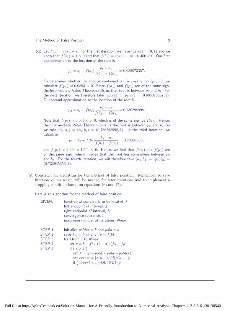
(d) Let f(x) = cos x− x. For the first iteration, we have (a1, b1) = (0, 1) and weknow that f(a1) = 1 > 0 and that f(b1) = cos 1− 1 ≈ −0.460 < 0. Our firstapproximation to the location of the root is
p1 = b1 − f(b1)b1 − a1
f(b1) − f(a1)= 0.685073357.
To determine whether the root is contained on (a1, p1) or on (p1, b1), wecalculate f(p1) ≈ 0.0893 > 0. Since f(a1) and f(p1) are of the same sign,the Intermediate Value Theorem tells us that root is between p1 and b1. Forthe next iteration, we therefore take (a2, b2) = (p1, b1) = (0.685073357, 1).Our second approximation to the location of the root is
p2 = b2 − f(b2)b2 − a2
f(b2) − f(a2)= 0.736298998.
Note that f(p2) ≈ 0.00466 > 0, which is of the same sign as f(a2). Hence,the Intermediate Value Theorem tells us the root is between p2 and b2, sowe take (a3, b3) = (p2, b2) = (0.736298998, 1). In the third iteration, wecalculate
p3 = b3 − f(b3)b3 − a3
f(b3) − f(a3)= 0.738945356
and f(p3) ≈ 2.339 × 10⁻⁴ < 0. Hence, we find that f(a3) and f(p3) areof the same sign, which implies that the root lies somewhere between p3
and b3. For the fourth iteration, we will therefore take (a4, b4) = (p3, b3) =(0.738945356, 1).
2. Construct an algorithm for the method of false position. Remember to savefunction values which will be needed for later iterations and to implement astopping condition based on equations (6) and (7).
Here is an algorithm for the method of false position:
GIVEN: function whose zero is to be located, f
left endpoint of interval, a
right endpoint of interval, b
convergence tolerance, ǫmaximum number of iterations, Nmax
STEP 1: initialize polder = b and pold = bSTEP 2: save fa = f(a) and fb = f(b)STEP 3: for i from 1 to Nmax
STEP 4: set p = b − fb ∗ (b − a)/(fb − fa)STEP 5: if ( i > 2 )
set λ = (p − pold)/(pold − polder)set errest = |λ(p − pold)/(λ − 1)|if ( errest < ǫ ) OUTPUT p
Full file at http://AplusTestbank.eu/Solution-Manual-for-A-Friendly-Introduction-to-Numerical-Analysis-Chapters-1-2-3-5-6-130130540

4 Section 2.2
endSTEP 6: save fp = f(p)STEP 7: if (sign(fa) ∗ sign(fp) < 0)
assign the value of p to b
assign the value of fp to fb
elseassign the value of p to a
assign the value of fp to fa
endSTEP 8: assign the value of pold to polder
assign the value of p to pold
endOUTPUT: “maximum number of iterations exceeded”
3. Confirm that |λ| < 1 for the remaining configurations in Figure 2-5.
Start with the configuration depicted in the upper right panel of Figure 2.5. Becausean is fixed, l = an−p. Now, an−p < 0 and f ′′(p) > 0, so (an−p)f ′′(p) < 0. Sincef ′(p) is also less than zero, it follows that 2f ′(p) + (an − p)f ′′(p) < (an − p)f ′′(p)and
0 <(an − p)f ′′(p)
2f ′(p) + (an − p)f ′′(p)= λ < 1.
Hence, |λ| < 1.
In the lower left panel of Figure 2.5, bn is fixed, so l = bn −p. Now, bn −p > 0 andf ′′(p) > 0, so (bn − p)f ′′(p) > 0. Since f ′(p) is also greater than zero, it followsthat 2f ′(p) + (bn − p)f ′′(p) > (bn − p)f ′′(p) and
0 <(bn − p)f ′′(p)
2f ′(p) + (bn − p)f ′′(p)= λ < 1.
Hence, |λ| < 1.
Finally, in the lower right panel of Figure 2.5, bn is fixed, so l = bn − p. Now,bn − p > 0 and f ′′(p) < 0, so (bn − p)f ′′(p) < 0. Since f ′(p) is also less than zero,it follows that 2f ′(p) + (bn − p)f ′′(p) < (bn − p)f ′′(p) and
0 <(bn − p)f ′′(p)
2f ′(p) + (bn − p)f ′′(p)= λ < 1.
Hence, |λ| < 1.
In Exercises 4 - 7, an equation, an interval on which the equation has a root,and the exact value of the root are specified.
Full file at http://AplusTestbank.eu/Solution-Manual-for-A-Friendly-Introduction-to-Numerical-Analysis-Chapters-1-2-3-5-6-130130540

The Method of False Position 5
(a) Perform the first five (5) iterations of the method of false position.(b) Verify that the absolute error in the third, fourth and fifth approximationssatisfies the error estimate
|pn − p| ≈∣
∣
∣
∣
λ
λ − 1
∣
∣
∣
∣
|pn − pn−1|.
(c) How does the error in the fifth false position approximation compare to themaximum error which would result from six iterations of the bisection method?
4. The equation x3 + x2 − 3x − 3 = 0 has a root on the interval (1, 2), namelyx =
√3.
The following table summarizes the results of five iterations of the method of falseposition with f(x) = x3 + x2 − 3x − 3 and (a1, b1) = (1, 2).
errorn pn |pn − p| estimate1 1.571429 0.1606222 1.705411 2.664 × 10⁻²
3 1.727883 4.168 × 10⁻³ 4.529 × 10⁻³
4 1.731405 6.459 × 10⁻⁴ 6.546 × 10⁻⁴
5 1.731951 9.995 × 10⁻⁵ 1.002 × 10⁻⁴
Note that the error in the fifth false position approximation, 9.995 × 10⁻⁵, is sub-stantially smaller than the maximum error which would result from six iterations ofthe bisection method, (2 − 1)/26 = 0.015625.
5. The equation x7 = 3 has a root on the interval (1, 2), namely x = 7√
3.
The following table summarizes the results of five iterations of the method of falseposition with f(x) = x7 − 3 and (a1, b1) = (1, 2).
errorn pn |pn − p| estimate1 1.015748 0.1541832 1.030366 0.1395653 1.043882 0.126049 0.1658744 1.056333 0.113598 0.1455565 1.067761 0.102169 0.127730
Note that the error in the fifth false position approximation, 0.102169, is an orderof magnitude larger than the maximum error which would result from six iterationsof the bisection method, (2 − 1)/26 = 0.015625.
6. The equation x3 − 13 = 0 has a root on the interval (2, 3), namely 3√
13.
The following table summarizes the results of five iterations of the method of falseposition with f(x) = x3 − 13 and (a1, b1) = (2, 3).
Full file at http://AplusTestbank.eu/Solution-Manual-for-A-Friendly-Introduction-to-Numerical-Analysis-Chapters-1-2-3-5-6-130130540

6 Section 2.2
errorn pn |pn − p| estimate1 2.263158 0.0881772 2.330507 0.0208273 2.346490 4.844 × 10⁻³ 4.973 × 10⁻³
4 2.350212 1.123 × 10⁻³ 1.130 × 10⁻³
5 2.351075 2.600 × 10⁻⁴ 2.604 × 10⁻⁴
Note that the error in the fifth false position approximation, 2.600 × 10⁻⁴, is sub-stantially smaller than the maximum error which would result from six iterations ofthe bisection method, (3 − 2)/26 = 0.015625.
7. The equation 1/x−37 = 0 has a zero on the interval (0.01, 0.1), namely x = 1/37.
The following table summarizes the results of five iterations of the method of falseposition with f(x) = 1
x− 37 and (a1, b1) = (0.01, 0.1).
errorn pn |pn − p| estimate1 0.073000 0.0459732 0.055990 0.0289633 0.045274 0.018247 0.0182474 0.038522 0.011495 0.0114955 0.034269 0.007242 0.007242
Note that the error in the fifth false position approximation, 0.007242, is nearly fivetimes larger than the maximum error which would result from six iterations of thebisection method, (0.1 − 0.01)/26 = 0.00140625.
8. The function f(x) = sinx has a zero on the interval (3, 4), namely x = π.Perform three iterations of the method of false position to approximate this zero.Determine the absolute error in each of the three computed approximations.What is the apparent order of convergence? What explanation can you providefor this behavior?
The following table summarizes the results of three iterations of the method of falseposition with f(x) = sinx and (a1, b1) = (3, 4).
n pn |pn − p|1 3.1571627924799466 1.557 × 10⁻²
2 3.1415462555891498 4.640 × 10⁻⁵
3 3.1415926554589646 1.869 × 10⁻⁹
Each error appears to be the square of the previous error, so the order of convergenceappears to be α = 2; i.e., quadratic convergence. The order of convergence for thisspecific problem is better than the expected linear convergence for the method of
Full file at http://AplusTestbank.eu/Solution-Manual-for-A-Friendly-Introduction-to-Numerical-Analysis-Chapters-1-2-3-5-6-130130540

The Method of False Position 7
false position because f ′′(π) = − sin π = 0; thus,
limn→∞
|en||en−1|
=lf ′′(π)
2f ′(π) + lf ′′(π)= 0,
which implies that convergence is better than linear.
9. (a) Verify that the equation x4−18x2+45 = 0 has a root on the interval (1, 2).Next, perform three iterations of the method of false position. Given thatthe exact value of the root is x =
√3, compute the absolute error in
the three approximations just obtained. What is the apparent order ofconvergence? What explanation can you provide for this behavior?
(b) Verify that the equation x4 − 18x2 + 45 = 0 also has a root on the interval(3, 4). Perform five iterations of the method of false position, and computethe absolute error in each approximation. The exact value of the root isx =
√15. What is the apparent order of convergence in this case?
(c) What explanation can you provide for the different convergence behaviorbetween parts (a) and (b)?
(a) Let f(x) = x4 −18x2 +45. Then f(1) = 28 > 0 and f(2) = −11 < 0, so theIntermediate Value Theorem guarantees the existence of a root on the interval(1, 2). With (a1, b1) = (1, 2), the following table summarizes the results ofthree iterations of the method of false position.
n pn |pn − p|1 1.717948717949 1.410 ×10⁻²
2 1.732218859330 1.681 ×10⁻⁴
3 1.732050802076 5.493 ×10⁻⁹
Convergence appears to be of order two (note that each error appears to bethe square of the previous error), which is better than expected for the methodof false position. This happens because f ′′(
√3) = 0; thus,
limn→∞
|en||en−1|
=lf ′′(
√3)
2f ′(√
3) + lf ′′(√
3)= 0,
which implies that convergence is better than linear.
(b) Let f(x) = x4 −18x2 +45. Then f(3) = −36 < 0 and f(4) = 13 > 0, so theIntermediate Value Theorem guarantees the existence of a root on the interval(3, 4). With (a1, b1) = (3, 4), the following table summarizes the results offive iterations of the method of false position.
n pn |pn − p|1 3.734693877551 1.383 ×10⁻¹
2 3.859328133794 1.366 ×10⁻²
3 3.871720773366 1.263 ×10⁻³
4 3.872867347773 1.160 ×10⁻⁴
5 3.872972695145 1.065 ×10⁻⁵
Full file at http://AplusTestbank.eu/Solution-Manual-for-A-Friendly-Introduction-to-Numerical-Analysis-Chapters-1-2-3-5-6-130130540
8 Section 2.2
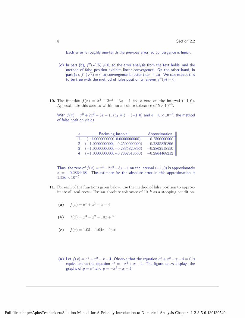
Each error is roughly one-tenth the previous error, so convergence is linear.
(c) In part (b), f ′′(√
15) 6= 0, so the error analysis from the text holds, and themethod of false position exhibits linear convergence. On the other hand, inpart (a), f ′′(
√3) = 0 so convergence is faster than linear. We can expect this
to be true with the method of false position whenever f ′′(p) = 0.
10. The function f(x) = x3 + 2x2 − 3x − 1 has a zero on the interval (−1, 0).Approximate this zero to within an absolute tolerance of 5× 10⁻⁵.
With f(x) = x3 + 2x2 − 3x − 1, (a1, b1) = (−1, 0) and ǫ = 5 × 10⁻⁵, the methodof false position yields
n Enclosing Interval Approximation1 (−1.0000000000, 0.0000000000) −0.25000000002 (−1.0000000000,−0.2500000000) −0.28358208963 (−1.0000000000,−0.2835820896) −0.28625185504 (−1.0000000000,−0.2862518550) −0.2864468212
Thus, the zero of f(x) = x3 +2x2−3x−1 on the interval (−1, 0) is approximatelyx = −0.2864468. The estimate for the absolute error in this approximation is1.536 × 10−5.
11. For each of the functions given below, use the method of false position to approx-imate all real roots. Use an absolute tolerance of 10−6 as a stopping condition.
(a) f(x) = ex + x2 − x − 4
(b) f(x) = x3 − x2 − 10x + 7
(c) f(x) = 1.05 − 1.04x + lnx
(a) Let f(x) = ex +x2 −x− 4. Observe that the equation ex +x2 −x− 4 = 0 isequivalent to the equation ex = −x2 + x + 4. The figure below displays thegraphs of y = ex and y = −x2 + x + 4.
Full file at http://AplusTestbank.eu/Solution-Manual-for-A-Friendly-Introduction-to-Numerical-Analysis-Chapters-1-2-3-5-6-130130540

The Method of False Position 9
The graphs appear to intersect over the intervals (−2,−1) and (1, 2). Usingeach of these intervals and a convergence tolerance of 10−6, the method offalse position yields
n (a1, b1) = (−2,−1) (a1, b1) = (1, 2)1 −1.4332155776 1.19213934092 −1.4977012853 1.25780826293 −1.5059259021 1.27895159124 −1.5069532761 1.28562776255 −1.5070812744 1.28772283166 −1.5070972162 1.28837901627 −1.5070992016 1.28858441098 1.28864869019 1.288668805310 1.288675099911 1.2886770697
Thus, the zeros of f(x) = ex +x2 −x− 4 are approximately x = −1.5070992and x = 1.2886771.
(b) Let f(x) = x3 − x2 − 10x + 7. By trial and error, we find that f(−4) < 0,f(−3) > 0, f(0) > 0, f(1) < 0, f(3) < 0 and f(4) > 0. Therefore, thethree real zeros of f lie on the intervals (−4,−3), (0, 1) and (3, 4). Using eachof these intervals and a convergence tolerance of 10−6, the method of falseposition yields
Full file at http://AplusTestbank.eu/Solution-Manual-for-A-Friendly-Introduction-to-Numerical-Analysis-Chapters-1-2-3-5-6-130130540

10 Section 2.2
n (a1, b1) = (−4,−3) (a1, b1) = (0, 1) (a1, b1) = (3, 4)1 −3.0294117647 0.7000000000 3.25000000002 −3.0385846418 0.6856023506 3.32773109243 −3.0414199487 0.6852297516 3.34943799584 −3.0422938990 0.6852204836 3.35531145015 −3.0425630528 3.35688697016 −3.0426459232 3.35730860847 −3.0426714363 3.35742137608 −3.0426792907 3.35745153079 −3.0426817088 3.357459594010 −3.0426824532 3.3574617500
Thus, the zeros of f(x) = x3−x2−10x+7 are approximately x = −3.0426825,x = 0.6852205 and x = 3.3574618.
(c) Let f(x) = 1.05−1.04x+ln x. Observe that the equation 1.05−1.04x+ln x =0 is equivalent to the equation lnx = 1.04x− 1.05. The figure below displaysthe graphs of y = lnx and y = 1.04x − 1.05.
The graphs appear to intersect over the intervals (0.80, 0.85) and (1.10, 1.15).Using each of these intervals and a convergence tolerance of 10−6, the methodof false position yields
n (a1, b1) = (0.80, 0.85) (a1, b1) = (1.10, 1.15)1 0.8298189963 1.10867871352 0.8274663932 1.10960533493 0.8272115742 1.10970126584 0.8271841999 1.10971116525 0.8271812617 1.1097121864
Thus, the zeros of f(x) = 1.05−1.04x+ln x are approximately x = 0.8271813and x = 1.1097122.
Full file at http://AplusTestbank.eu/Solution-Manual-for-A-Friendly-Introduction-to-Numerical-Analysis-Chapters-1-2-3-5-6-130130540

The Method of False Position 11
12. In the literature, it is not uncommon to find the method of false position ter-minated when |pn − pn−1| < ǫ. Comment on the accuracy of this stoppingcondition. Consider the cases λ ≈ 0, λ ≈ 1/2 and λ ≈ 1.
Recall that
|pn − p| ≈∣
∣
∣
∣
λ
λ − 1
∣
∣
∣
∣
|pn − pn−1|.
If λ ≈ 0, then |pn − p| is much smaller than |pn − pn−1|. In this case, using astopping condition based on |pn − pn−1| < ǫ is overly pessimistic and will result inmore iterations being performed than are necessary to achieve the desired accuracy.If λ ≈ 1/2, then λ/(λ− 1) ≈ 1 and |pn −p| ≈ |pn −pn−1|. In this case, a stoppingcondition based on |pn − pn−1| < ǫ is acceptable. Finally, suppose λ ≈ 1. Thenλ/(λ− 1) → ∞ and |pn − p| is much larger than |pn − pn−1|. In this case, using astopping condition based on |pn − pn−1| < ǫ is overly optimistic and will result intermination before the desired accuracy has been achieved.
13. A storage tank is in the shape of a horizontal cylinder with length L and radiusr. The volume V of fluid in the tank is related to the depth h of the fluid bythe equation
V =
[
r2 cos−1
(
r − h
r
)
− (r − h)√
2rh − h2
]
L.
If r = 1 meter, L = 3 meters and V = 7 cubic meters, determine h.
Because the radius of the tank is one meter, we are guaranteed that 0 ≤ h ≤ 2.Applying the method of false position to the function
f(h) = 3(
cos−1(1 − h) − (1 − h)√
2h − h2
)
− 7
with a starting interval of (a1, b1) = (0, 2) and a convergence tolerance of 5×10⁻⁵
yields
n Enclosing Interval Approximation1 (0.0000000000,2.0000000000) 1.48544613552 (0.0000000000,1.4854461355) 1.38526437913 (1.3852643791,1.4854461355) 1.39166569334 (1.3852643791,1.3916656933) 1.3915144154
Thus, if the tank contains 7 cubic meters of fluid, it is filled to a depth of approxi-mately h = 1.39 meters.
14. The equation x2 = 1 − cos(√
2x) +√
2 sin(√
2x) has two real roots. One ofthem is at x = 0. Determine an interval which contains the other root, andthen approximate this root to three decimal places. This problem arises in thecalculation of the amplitude of the solution to a nonlinear third-order differ-ential equation. See Gottlieb (“Simple nonlinear jerk functions with periodicsolutions,” American Journal of Physics, 66 (10), 903 - 906, 1998) for details.
Full file at http://AplusTestbank.eu/Solution-Manual-for-A-Friendly-Introduction-to-Numerical-Analysis-Chapters-1-2-3-5-6-130130540

12 Section 2.2
Letf(x) = x2 − 1 + cos(
√2x) −
√2 sin(
√2x).
Because f(1) ≈ −1.241 < 0 and f(2) ≈ 1.613 > 0, we know the other root of f
lies on the interval (1, 2). Applying the method of false position to f with a startinginterval of (a1, b1) = (1, 2) and a convergence tolerance of 5 × 10⁻⁴ yields
n Enclosing Interval Approximation1 (1.0000000000,2.0000000000) 1.43482848872 (1.4348284887,2.0000000000) 1.59751789503 (1.5975178950,2.0000000000) 1.63698880584 (1.6369888058,2.0000000000) 1.64533923665 (1.6453392366,2.0000000000) 1.6470507507
Thus, the other root of x2 = 1 − cos(√
2x) +√
2 sin(√
2x) is approximately x =1.647.
15. Rework the “Depth of Submersion” problem to determine the depth to which aglass marble of radius 2 cm and density 0.040 g/cm3 sinks in water of density0.998 g/cm3.
When a spherical object of radius R and density ρo is placed on the surface of afluid of density ρf , it will sink to a depth h that is a root of the equation
ρf
3h3 − Rρfh2 +
4
3R3ρo = 0.
If a glass marble of radius 2 cm and density 0.040 g/cm3 is placed in water ofdensity 0.998 g/cm3, then h is a root of the equation
0.998
3h3 − 1.996h2 +
1.28
3= 0.
The method of false position with a starting interval of (0, 4) and a convergencetolerance of 5 × 10⁻⁵ yields
n Enclosing Interval Approximation1 (0.0000000000,4.0000000000) 0.16032064132 (0.1603206413,4.0000000000) 0.29684601113 (0.2968460111,4.0000000000) 0.38855259154 (0.3885525915,4.0000000000) 0.43902566855 (0.4390256685,4.0000000000) 0.46328770626 (0.4632877062,4.0000000000) 0.47409931957 (0.4740993195,4.0000000000) 0.47874285208 (0.4787428520,4.0000000000) 0.48070453659 (0.4807045365,4.0000000000) 0.481527381810 (0.4815273818,4.0000000000) 0.481871493511 (0.4818714935,4.0000000000) 0.482015218312 (0.4820152183,4.0000000000) 0.4820752160
Full file at http://AplusTestbank.eu/Solution-Manual-for-A-Friendly-Introduction-to-Numerical-Analysis-Chapters-1-2-3-5-6-130130540

The Method of False Position 13
Thus, the marble will sink to a depth of approximately h = 0.482 cm.
Full file at http://AplusTestbank.eu/Solution-Manual-for-A-Friendly-Introduction-to-Numerical-Analysis-Chapters-1-2-3-5-6-130130540

Fixed Point Iteration Schemes 1
2.3 Fixed Point Iteration Schemes
1. Suppose the sequence {pn} is generated by the fixed point iteration schemepn = g(pn−1). Further, suppose that the sequence converges linearly to thefixed point p.
(a) Show that
g′(p) ≈ pn − pn−1
pn−1 − pn−2.
(b) Show that
|en| ≈∣
∣
∣
∣
g′(p)
g′(p) − 1
∣
∣
∣
∣
|pn − pn−1|.
Suppose the sequence {pn}, generated by the fixed point iteration scheme pn =g(pn−1), converges linearly to the fixed point p.
(a) By the Mean Value Theorem,
pn − pn−1 = g(pn−1) − g(pn−2)
= g′(ξ)(pn−1 − pn−2)
where ξ is between pn−1 and pn−2. As n increases, pn−1 and pn−2 both tendtoward p, so by the squeeze theorem, ξ also tends toward p. Hence,
pn − pn−1
pn−1 − pn−2= g′(ξ) ≈ g′(p).
(b) Recall that when a fixed point iteration scheme converges linearly the asymp-totic error constant is λ = g′(p). Thus, en ≈ g′(p)en−1, or en−1 ≈ en/g′(p).Now,
en = p − pn
= pn − pn−1 + pn−1 − p
= pn − pn−1 + en−1.
Substituting en−1 ≈ en/g′(p) into this last expression, solving for en, andtaking absolute values yields
|en| ≈∣
∣
∣
∣
g′(p)
g′(p) − 1
∣
∣
∣
∣
|pn − pn−1|.
Full file at http://AplusTestbank.eu/Solution-Manual-for-A-Friendly-Introduction-to-Numerical-Analysis-Chapters-1-2-3-5-6-130130540
2 Section 2.3
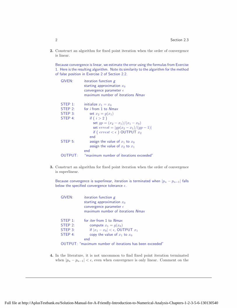
2. Construct an algorithm for fixed point iteration when the order of convergenceis linear.
Because convergence is linear, we estimate the error using the formulas from Exercise1. Here is the resulting algorithm. Note its similarity to the algorithm for the methodof false position in Exercise 2 of Section 2.2.
GIVEN: iteration function g
starting approximation x0
convergence parameter ǫmaximum number of iterations Nmax
STEP 1: initialize x1 = x0
STEP 2: for i from 1 to Nmax
STEP 3: set x2 = g(x1)STEP 4: if ( i > 2 )
set gp = (x2 − x1)/(x1 − x0)set errest = |gp(x2 − x1)/(gp − 1)|if ( errest < ǫ ) OUTPUT x2
endSTEP 5: assign the value of x1 to x0
assign the value of x2 to x1
endOUTPUT: “maximum number of iterations exceeded”
3. Construct an algorithm for fixed point iteration when the order of convergenceis superlinear.
Because convergence is superlinear, iteration is terminated when |pn − pn−1| fallsbelow the specified convergence tolerance ǫ.
GIVEN: iteration function g
starting approximation x0
convergence parameter ǫmaximum number of iterations Nmax
STEP 1: for iter from 1 to Nmax
STEP 2: compute x1 = g(x0)STEP 3: if |x1 − x0| < ǫ, OUTPUT x1
STEP 4: copy the value of x1 to x0
endOUTPUT: “maximum number of iterations has been exceeded”
4. In the literature, it is not uncommon to find fixed point iteration terminatedwhen |pn − pn−1| < ǫ, even when convergence is only linear. Comment on the
Full file at http://AplusTestbank.eu/Solution-Manual-for-A-Friendly-Introduction-to-Numerical-Analysis-Chapters-1-2-3-5-6-130130540
Fixed Point Iteration Schemes 3
accuracy of this stopping condition when convergence is linear. Consider thecases g′(p) ≈ 0, g′(p) ≈ 1/2 and g′(p) ≈ 1.
Recall that when convergence is linear
|pn − p| ≈∣
∣
∣
∣
g′(p)
g′(p) − 1
∣
∣
∣
∣
|pn − pn−1|.
If g′(p) ≈ 0, then |pn − p| is much smaller than |pn − pn−1|. In this case, using astopping condition based on |pn − pn−1| < ǫ is overly pessimistic and will result inmore iterations being performed than are necessary to achieve the desired accuracy.If g′(p) ≈ 1/2, then g′(p)/(g′(p) − 1) ≈ 1 and |pn − p| ≈ |pn − pn−1|. In thiscase, a stopping condition based on |pn − pn−1| < ǫ is acceptable. Finally, supposeg′(p) ≈ 1. Then g′(p)/(g′(p)−1) → ∞ and |pn−p| is much larger than |pn−pn−1|.In this case, using a stopping condition based on |pn−pn−1| < ǫ is overly optimisticand will result in termination before the desired accuracy has been achieved.
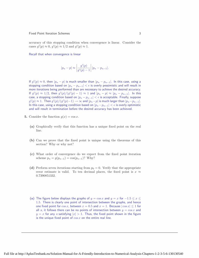
5. Consider the function g(x) = cos x.
(a) Graphically verify that this function has a unique fixed point on the realline.
(b) Can we prove that the fixed point is unique using the theorems of thissection? Why or why not?
(c) What order of convergence do we expect from the fixed point iterationscheme pn = g(pn−1) = cos(pn−1)? Why?
(d) Perform seven iterations starting from p0 = 0. Verify that the appropriateerror estimate is valid. To ten decimal places, the fixed point is x ≈0.7390851332.
(a) The figure below displays the graphs of y = cos x and y = x for −1.5 ≤ x ≤1.5. There is clearly one point of intersection between the graphs, and henceone fixed point for cos x, between x = 0.5 and x = 1. Because | cos x| ≤ 1 forall x, it follows there can be no points of intersection between y = cos x andy = x for any x satisfying |x| > 1. Thus, the fixed point shown in the figureis the unique fixed point of cos x on the entire real line.
Full file at http://AplusTestbank.eu/Solution-Manual-for-A-Friendly-Introduction-to-Numerical-Analysis-Chapters-1-2-3-5-6-130130540

4 Section 2.3
(b) Because there is no k < 1 such that |g′(x)| ≤ k for all real numbers x, wecannot use the theorems of this section to prove that the fixed point is unique.
(c) In the figure from part (a), we see that at the point of intersection betweenthe graphs of y = cos x and y = x, the tangent line to the graph of y = cos xis not horizontal. In other words, if p denotes the fixed point of g(x) = cos x,then g′(p) 6= 0. Since g′(p) 6= 0, convergence of the sequence generated bythe fixed point iteration scheme pn = g(pn−1) will be linear.
(d) Because we expect linear convergence, the appropriate error estimate is
|en| ≈∣
∣
∣
∣
g′(p)
g′(p) − 1
∣
∣
∣
∣
|pn − pn−1|
where
g′(p) ≈ pn − pn−1
pn−1 − pn−2.
Here are the results of seven iterations of the fixed point scheme starting fromp0 = 0.
theoreticaln pn |pn − p| error estimate1 1.0000000000 0.26091486682 0.5403023059 0.19878282733 0.8575532158 0.1184680826 0.1295428543794 0.6542897905 0.0847953427 0.0793753740875 0.7934803587 0.0543952255 0.0565740644026 0.7013687736 0.0377163596 0.0366816477497 0.7639596829 0.0248745497 0.025323586019
6. Consider the function g(x) = 1 + x − 18x3.
(a) Analytically verify that this function has a unique fixed point on the realline.
Full file at http://AplusTestbank.eu/Solution-Manual-for-A-Friendly-Introduction-to-Numerical-Analysis-Chapters-1-2-3-5-6-130130540

Fixed Point Iteration Schemes 5
(b) Can we prove that the fixed point is unique using the theorems of thissection? Why or why not?
(c) What order of convergence do we expect from the fixed point iterationscheme pn = g(pn−1)? Why?
(d) Perform seven iterations starting from p0 = 0. Verify that the appropriateerror estimate is valid.
(a) The equation 1+x− 18x3 = x is equivalent to x3 = 8. The only real solution of
this last equation is x = 2; therefore, the only fixed point of g(x) = 1+x− 18x3
on the real line is x = 2.
(b) Because there is no k < 1 such that |g′(x)| ≤ k for all real numbers x, wecannot use the theorems of this section to prove that the fixed point is unique.
(c) Note that
g′(2) =
(
1 − 3
8x2
)∣
∣
∣
∣
x=2
= −1
26= 0.
Since g′(2) 6= 0, convergence of the sequence generated by the fixed pointiteration scheme pn = g(pn−1) will be linear.
(d) Because we expect linear convergence, the appropriate error estimate is
|en| ≈∣
∣
∣
∣
g′(p)
g′(p) − 1
∣
∣
∣
∣
|pn − pn−1|
where
g′(p) ≈ pn − pn−1
pn−1 − pn−2.
Here are the results of seven iterations of the fixed point scheme starting fromp0 = 0.
theoreticaln pn |pn − p| error estimate1 1.0000000000 1.00000000002 1.8750000000 0.12500000003 2.0510253906 0.0510253906 0.0443291326024 1.9725180057 0.0274819943 0.0242146005705 2.0131771467 0.0131771467 0.0138727359326 1.9932809128 0.0067190872 0.0065371591537 2.0033257219 0.0033257219 0.003369895664
7. Consider the function g(x) = 2x(1− x), which has fixed points at x = 0 and atx = 1/2.
(a) Why should we expect that fixed point iteration, starting even with a valuevery close to zero, will fail to converge toward x = 0?
Full file at http://AplusTestbank.eu/Solution-Manual-for-A-Friendly-Introduction-to-Numerical-Analysis-Chapters-1-2-3-5-6-130130540

6 Section 2.3
(b) Why should we expect that fixed point iteration, starting with p0 ∈ (0, 1)will converge toward x = 1/2? What order of convergence should weexpect?
(c) Perform seven iterations starting from an arbitrary p0 ∈ (0, 1) and numer-ically confirm the order of convergence.
(a) Note that g′(0) = 2 > 1. Thus, for x ≈ 0,
g(x) ≈ g(0) + g′(0)x = 2x.
If we choose a starting value very close to 0, it follows that each new term inthe sequence pn = g(pn−1) will be roughly twice the previous term. In otherwords, the terms in the sequence will be moving further from 0, not convergingtoward 0.
(b) Due to the symmetry of g about x = 1/2, we can restrict attention to p0 ∈(0, 1/2). Since |g′(x)| < 1 for 1/4 < x < 1/2, it follows from the theorems ofthis section that the iteration will converge for any p0 ∈ (1/4, 1/2). Finally,since g′(x) ≥ 1 for 0 < x ≤ 1/4, it follows that for any p0 ∈ (0, 1/4), pn
will eventually lie in (1/4, 1/2) and the iteration will converge to 1/2. Sinceg′(1/2) = 0, but g′′(1/2) 6= 0, convergence will be quadratic.
(c) Here are the results of seven iterations of the fixed point iteration schemestarting from p0 = 0.1. From the values in the fourth column of the tablebelow, we observe that the ratio
|pn − p||pn−1 − p|2
approaches a constant, thereby confirming that convergence is quadratic.
n pn |pn − p| |pn − p|/|pn−1 − p|20 0.1000000000000000 4.000 ×10⁻¹
1 0.1800000000000000 3.800 ×10⁻¹ 2.3752 0.2952000000000000 2.048 ×10⁻¹ 1.4183 0.4161139200000000 8.389 ×10⁻² 2.0004 0.4859262511644672 1.407 ×10⁻² 1.9995 0.4996038591874287 3.961 ×10⁻⁴ 2.0006 0.4999996861449132 3.139 ×10⁻⁷ 2.0017 0.4999999999998030 1.970 ×10⁻¹³ 1.999
8. Verify that x =√
a is a fixed point of the function
g(x) =1
2
(
x +a
x
)
.
Use the techniques of this section to determine the order of convergence and theasymptotic error constant of the sequence pn = g(pn−1) toward x =
√a.
Full file at http://AplusTestbank.eu/Solution-Manual-for-A-Friendly-Introduction-to-Numerical-Analysis-Chapters-1-2-3-5-6-130130540
Fixed Point Iteration Schemes 7
Let
g(x) =1
2
(
x +a
x
)
,
and note that
g(√
a) =1
2
(√a +
a√a
)
=1
2(√
a +√
a) =√
a.
Thus, x =√
a is a fixed point of g. To determine the order of convergence and theasymptotic error constant for the sequence pn = g(pn−1), we need to examine thevalues of the derivatives of g at x =
√a. Now
g′(x) =1
2
(
1 − a
x2
)
so g′(√
a) =1
2
(
1 − a
a
)
= 0.
The order of convergence is therefore at least 2. Because
g′′(x) =a
x3and g′′(
√a) =
1√a6= 0,
the order of convergence is exactly 2. Furthermore, the asymptotic error constantis
λ =|g′′(√a)|
2!=
1
2√
a.
9. Verify that x =√
a is a fixed point of the function
g(x) =x3 + 3xa
3x2 + a.
Use the techniques of the this section to determine the order of convergence andthe asymptotic error constant of the sequence pn = g(pn−1) toward x =
√a.
Let
g(x) =x3 + 3xa
3x2 + a,
and note that
g(√
a) =a√
a + 3a√
a
3a + a=
4a√
a
4a=
√a.
Thus, x =√
a is a fixed point of g. To determine the order of convergence and theasymptotic error constant for the sequence pn = g(pn−1), we need to examine thevalues of the derivatives of g at x =
√a. Now
g′(x) =3(x4 − 2x2a + a2)
(3x2 + a)2so g′(
√a) =
3(a2 − 2a2 + a2)
(4a)2= 0.
The order of convergence is therefore at least 2. Because
g′′(x) =48xa(x2 − a)
(3x2 + a)3and g′′(
√a) =
48a√
a(a − a)
(4a)3= 0,
Full file at http://AplusTestbank.eu/Solution-Manual-for-A-Friendly-Introduction-to-Numerical-Analysis-Chapters-1-2-3-5-6-130130540

8 Section 2.3
the order of convergence is at least 3. Finally,
g′′′(x) = −48a(9x4 − 18x2a + a2)
(3x2 + a)4
and
g′′′(√
a) = −48a(9a2 − 18a2 + a2)
(4a)4=
3
2a,
so the order of convergence is exactly 3. Furthermore, the asymptotic error constantis
λ =|g′′′(√a)|
3!=
1
4a.
10. Verify that x = 1/a is a fixed point of the function g(x) = x(2 − ax). Use thetechniques of the this section to determine the order of convergence and theasymptotic error constant of the sequence pn = g(pn−1) toward x = 1/a.
Let g(x) = x(2 − ax), and note that
g
(
1
a
)
=1
a
(
2 − a · 1
a
)
=1
a.
Thus, x = 1a is a fixed point of g. To determine the order of convergence and the
asymptotic error constant for the sequence pn = g(pn−1), we need to examine thevalues of the derivatives of g at x = 1
a . Now
g′(x) = 2 − 2ax so g′(
1
a
)
= 2 − 2a · 1
a= 0.
The order of convergence is therefore at least 2. Because
g′′(x) = −2a and g′′(
1
a
)
= −2a 6= 0,
the order of convergence is exactly 2. Furthermore, the asymptotic error constantis
λ =|g′′(
1a
)
|2!
= a.
11. Consider the function g(x) = e−x2
.
(a) Prove that g has a unique fixed point on the interval [0, 1].
(b) With a starting approximation of p0 = 0, use the iteration scheme pn =
e−p2
n−1 to approximate the fixed point on [0, 1] to within 5 × 10⁻⁷.
Full file at http://AplusTestbank.eu/Solution-Manual-for-A-Friendly-Introduction-to-Numerical-Analysis-Chapters-1-2-3-5-6-130130540

Fixed Point Iteration Schemes 9
(c) Use the theoretical error bound |pn − p| ≤ kn
1−k |p1 − p0| to obtain a theo-retical bound on the number of iterations needed to approximate the fixedpoint to within 5× 10⁻⁷. How does the number of iterations performed inpart (b) compare with the theoretical bound?
(a) Let g(x) = e−x2
. We will proceed by showing that g is continuous on [0, 1],maps [0, 1] to [0, 1] and there exists a k < 1 such that |g′(x)| ≤ k for allx ∈ [0, 1]. First, note that g is the composition of the functions ex and
−x2, both of which are continuous on [0, 1]. Consequently, g(x) = e−x2
iscontinuous on [0, 1]. Next, we see that
g′(x) = −2xe−x2
< 0
for all x ∈ (0, 1). Hence, g is decreasing on (0, 1). Combining this factwith g(0) = 1 and g(1) = e−1 ≈ 0.368, it then follows that for x ∈ [0, 1],g(x) ∈ [e−1, 1] ⊂ [0, 1]. Finally, we find
g′′(x) = (4x2 − 2)e−x2
= 0
when x =√
2/2. Because
g′(0) = 0, g′
(√2
2
)
= −√
2e−1/2 ≈ −0.858,
and g′(1) = −2e−1 ≈ −0.736, we find that |g′(x)| ≤√
2e−1/2 for all x ∈[0, 1]. Thus, we take k =
√2e−1/2. Having established that g is continuous
on [0, 1], maps [0, 1] to [0, 1] and there exists a k < 1 such that |g′(x)| ≤ kfor all x ∈ [0, 1], we conclude that g has a unique fixed point on the interval[0, 1].
(b) With a starting approximation of p0 = 0 and a convergence tolerance of ǫ =
5 × 10⁻⁷, fixed point iteration using g(x) = e−x2
yields p84 = 0.6529181524with an error estimate of 4.880 × 10⁻⁷.
(c) In part (a) we found k =√
2e−1/2. With p0 = 0, it follows that p1 = g(p0) =e0 = 1. Solving the equation
kn
1 − k|p1 − p0| ≤ 5 × 10⁻⁷
for n yields n ≥ 107.28, or, since n must be an integer, n ≥ 108. As thesecalculations were carried out using
k = maxx∈[0,1]
|g′(x)|,
we see that the upper bound on the number of iterations needed to guaranteean absolute error less than 5 × 10⁻⁷ is n = 108. In part (b), we found thatonly 84 iterations were needed to achieve the prescribed level of accuracy,confirming the theoretical upper bound.
Full file at http://AplusTestbank.eu/Solution-Manual-for-A-Friendly-Introduction-to-Numerical-Analysis-Chapters-1-2-3-5-6-130130540
10 Section 2.3
12. Repeat Exercise 11 for the function g(x) = 12 cos x.
(a) Let g(x) = 12 cos x. We will proceed by showing that g is continuous on [0, 1],
maps [0, 1] to [0, 1] and there exists a k < 1 such that |g′(x)| ≤ k for allx ∈ [0, 1]. First, note that g is a constant multiple of the function cos x,which is continuous on [0, 1]. Consequently, g(x) = 1
2 cos x is continuous on[0, 1]. Next, because (0, 1) ⊂ (0, π/2), we see that
g′(x) = −1
2sin x < 0
for all x ∈ (0, 1). Hence, g is decreasing on (0, 1). Combining this fact withg(0) = 1
2 and g(1) = 12 cos 1 ≈ 0.270, it then follows that for x ∈ [0, 1],
g(x) ∈ [ 12 cos 1, 12 ] ⊂ [0, 1]. Finally, we find
g′′(x) = −1
2cos x < 0
for all x ∈ [0, 1]. Because
g′(0) = 0 and g′(1) = −1
2sin 1 ≈ −0.421,
we find that |g′(x)| ≤ 12 sin 1 for all x ∈ [0, 1]. Thus, we take k = 1
2 sin 1.Having established that g is continuous on [0, 1], maps [0, 1] to [0, 1] and thereexists a k < 1 such that |g′(x)| ≤ k for all x ∈ [0, 1], we conclude that g hasa unique fixed point on the interval [0, 1].
(b) With a starting approximation of p0 = 0 and a convergence tolerance of ǫ =5× 10⁻⁷, fixed point iteration using g(x) = 1
2 cos x yields p9 = 0.4501838716with an error estimate of 2.603 × 10⁻⁷.
(c) In part (a) we found k = 12 sin 1. With p0 = 0, it follows that p1 = g(p0) =
12 cos 0 = 1
2 . Solving the equation
kn
1 − k|p1 − p0| ≤ 5 × 10⁻⁷
for n yields n ≥ 16.59, or, since n must be an integer, n ≥ 17. As thesecalculations were carried out using
k = maxx∈[0,1]
|g′(x)|,
we see that the upper bound on the number of iterations needed to guaranteean absolute error less than 5×10⁻⁷ is n = 17. In part (b), we found that only9 iterations were needed to achieve the prescribed level of accuracy, confirmingthe theoretical upper bound.
13. Repeat Exercise 11 for the function g(x) = 13 (2 − ex + x2).
Full file at http://AplusTestbank.eu/Solution-Manual-for-A-Friendly-Introduction-to-Numerical-Analysis-Chapters-1-2-3-5-6-130130540

Fixed Point Iteration Schemes 11
(a) Let g(x) = 13 (2 − ex + x2). We will proceed by showing that g is continuous
on [0, 1], maps [0, 1] to [0, 1] and there exists a k < 1 such that |g′(x)| ≤ kfor all x ∈ [0, 1]. First, note that g is a constant multiple of the sum of thefunctions 2, −ex, and x2, all of which are continuous on [0, 1]. Consequently,
g(x) = e−x2
is continuous on [0, 1]. Next, we see that
g′(x) =1
3(2x − ex) < 0
for all x ∈ (0, 1). Hence, g is decreasing on (0, 1). Combining this fact withg(0) = 1
3 and g(1) = 1 − 13e ≈ 0.0939, it then follows that for x ∈ [0, 1],
g(x) ∈ [1 − 13e, 1
3 ] ⊂ [0, 1]. Finally, we find
g′′(x) =1
3(2 − ex) = 0
when x = ln 2. Because
g′(0) = −1
3, g′(ln 2) =
2
3(ln 2 − 1) ≈ −0.205,
and g′(1) = 13 (2 − e) ≈ −0.239, we find that |g′(x)| ≤ 1
3 for all x ∈ [0, 1].Thus, we take k = 1
3 . Having established that g is continuous on [0, 1], maps[0, 1] to [0, 1] and there exists a k < 1 such that |g′(x)| ≤ k for all x ∈ [0, 1],we conclude that g has a unique fixed point on the interval [0, 1].
(b) With a starting approximation of p0 = 0 and a convergence tolerance ofǫ = 5 × 10⁻⁷, fixed point iteration using g(x) = 1
3 (2 − ex + x2) yields p10 =0.2575298907 with an error estimate of 3.947 × 10⁻⁷.
(c) In part (a) we found k = 13 . With p0 = 0, it follows that p1 = g(p0) =
13 (2 − e0 + 0) = 1
3 . Solving the equation
kn
1 − k|p1 − p0| ≤ 5 × 10⁻⁷
for n yields n ≥ 12.58, or, since n must be an integer, n ≥ 13. As thesecalculations were carried out using
k = maxx∈[0,1]
|g′(x)|,
we see that the upper bound on the number of iterations needed to guaranteean absolute error less than 5 × 10⁻⁷ is n = 13. In part (b), we found thatonly 10 iterations were needed to achieve the prescribed level of accuracy,confirming the theoretical upper bound.
14. The function f(x) = ex + x2 − x − 4 has a unique zero on the interval (1, 2).Create three different iteration functions corresponding to this function, andcompare their convergence properties for approximating the zero on (1, 2). Usethe same starting approximation, p0, for each iteration function.
Full file at http://AplusTestbank.eu/Solution-Manual-for-A-Friendly-Introduction-to-Numerical-Analysis-Chapters-1-2-3-5-6-130130540
12 Section 2.3
Answers will of course vary. Here are two possibilities. If we rearrange the equationex + x2 − x − 4 = 0 as
ex = 4 + x − x2
x = ln(4 + x − x2)
we may take g(x) = ln(4 + x − x2). With p0 = 1 and a convergence toleranceof 5 × 10⁻⁷, fixed point iteration yields p16 = 1.2886775801. Alternately, if werearrange ex + x2 − x − 4 = 0 as
x2 = 4 + x − ex
x =4 + x − ex
x
we may take g(x) = (4+x−ex)/x. Again using p0 = 1 and a convergence toleranceof 5 × 10⁻⁷, fixed point iteration fails to achieve convergence after 100 iterations.
15. Repeat Exercise 14 for the function f(x) = x3 − x2 − 10x + 7 on the interval(0, 1).
Answers will of course vary. Here are two possibilities. If we rearrange the equationx3 − x2 − 10x + 7 = 0 as
10x = x3 − x2 + 7
x =x3 − x2 + 7
10
we may take g(x) = (x3 − x2 + 7)/10. With p0 = 1 and a convergence toleranceof 5 × 10⁻⁷, fixed point iteration yields p3 = 0.6852205522. Alternately, if werearrange the equation x3 − x2 − 10x + 7 = 0 as
x3 = x2 + 10x − 7
x =x2 + 10x77
x2
we may take g(x) = (x2 + 10x − 7)/x2. Again using p0 = 1 and a convergencetolerance of 5 × 10⁻⁷, fixed point iteration yields p23 = 3.3574628337, which isoutside the interval (0, 1).
16. Repeat Exercise 14 for the function f(x) = 1.05 − 1.04x + lnx on the interval(1, 2).
Answers will of course vary. Here are two possibilities. If we rearrange the equation1.05 − 1.04x + lnx = 0 as
1.04x = 1.05 + lnx
x =1.05 + lnx
1.04
Full file at http://AplusTestbank.eu/Solution-Manual-for-A-Friendly-Introduction-to-Numerical-Analysis-Chapters-1-2-3-5-6-130130540

Fixed Point Iteration Schemes 13
we may take g(x) = (1.05 + lnx)/1.04. With p0 = 1 and a convergence toleranceof 5 × 10⁻⁷, fixed point iteration yields p90 = 1.1097118656. Alternately, if werearrange the equation 1.05 − 1.04x + lnx = 0 as
lnx = 1.04x − 1.05
x = e1.04x−1.05
we may take g(x) = e1.04x−1.05. Again using p0 = 1 and a convergence toleranceof 5 × 10⁻⁷, fixed point iteration yields p92 = 0.8271813610, which is outside theinterval (1, 2).
Full file at http://AplusTestbank.eu/Solution-Manual-for-A-Friendly-Introduction-to-Numerical-Analysis-Chapters-1-2-3-5-6-130130540
Newton’s Method 1
2.4 Newton’s Method
1. Each of the following equations has a root on the interval (0, 1). Perform New-ton’s method to determine p4, the fourth approximation to the location of theroot.
(a) ln(1 + x) − cos x = 0 (b) x5 + 2x − 1 = 0(c) e−x − x = 0 (d) cos x − x = 0
(a) Let f(x) = ln(1 + x) − cos x. Then f ′(x) = 1
1+x + sin x. With p0 = 0, fouriterations of Newton’s method yield
p1 = p0 −ln(1 + p0) − cos p0
1
1+p0
+ sin p0
= 1.0000000000;
p2 = p1 −ln(1 + p1) − cos p1
1
1+p1
+ sin p1
= 0.8860617364;
p3 = p2 −ln(1 + p2) − cos p2
1
1+p2
+ sin p2
= 0.8845109403; and
p4 = p3 −ln(1 + p3) − cos p3
1
1+p3
+ sin p3
= 0.8845106162.
(b) Let f(x) = x5 + 2x − 1. Then f ′(x) = 5x4 + 2. With p0 = 0, four iterationsof Newton’s method yield
p1 = p0 −p50 + 2p0 − 1
5p40 + 2
= 0.5000000000;
p2 = p1 −p51 + 2p1 − 1
5p41 + 2
= 0.4864864865;
p3 = p2 −p52 + 2p2 − 1
5p42 + 2
= 0.4863890407; and
p4 = p3 −p53 + 2p3 − 1
5p43 + 2
= 0.4863890359.
(c) Let f(x) = e−x − x. Then f ′(x) = −e−x − 1. With p0 = 0, four iterationsof Newton’s method yield
p1 = p0 −e−p0 − p0
−e−p0 − 1= 0.5000000000;
Full file at http://AplusTestbank.eu/Solution-Manual-for-A-Friendly-Introduction-to-Numerical-Analysis-Chapters-1-2-3-5-6-130130540

2 Section 2.4
p2 = p1 −e−p1 − p1
−e−p1 − 1= 0.5663110032;
p3 = p2 −e−p2 − p2
−e−p2 − 1= 0.5671431650; and
p4 = p3 −e−p3 − p3
−e−p3 − 1= 0.5671432904.
(d) Let f(x) = cos x− x. Then f ′(x) = − sin x− 1. With p0 = 0, four iterationsof Newton’s method yield
p1 = p0 −cos p0 − p0
− sin p0 − 1= 1.0000000000;
p2 = p1 −cos p1 − p1
− sin p1 − 1= 0.7503638678;
p3 = p2 −cos p2 − p2
− sin p2 − 1= 0.7391128909; and
p4 = p3 −cos p3 − p3
− sin p3 − 1= 0.7390851334.
2. Construct an algorithm for Newton’s method. Is it necessary to save all calcu-lated terms in the sequence {pn}?
Because convergence is quadratic, iteration is terminated when |pn − pn−1| fallsbelow the specified convergence tolerance ǫ. Note that only the two most recentterms in the sequence are needed.
GIVEN: function whose zero is to be located, f
starting approximation x0
convergence parameter ǫmaximum number of iterations Nmax
STEP 1: for iter from 1 to Nmax
STEP 2: compute x1 = x0 − f(x0)/f ′(x0)STEP 3: if |x1 − x0| < ǫ, OUTPUT x1
STEP 4: copy the value of x1 to x0
endOUTPUT: “maximum number of iterations has been exceeded”
In Exercises 3 - 6, an equation, an interval on which the equation has a root,and the exact value of the root are specified.(a) Perform five (5) iterations of Newton’s method.(b) For n ≥ 1, compare |pn − pn−1| with |pn−1 − p| and |pn − p|.(c) For n ≥ 1, compute the ratio |pn − p|/|pn−1 − p|2 and show that this valueapproaches |f ′′(p)/2f ′(p)|.
Full file at http://AplusTestbank.eu/Solution-Manual-for-A-Friendly-Introduction-to-Numerical-Analysis-Chapters-1-2-3-5-6-130130540
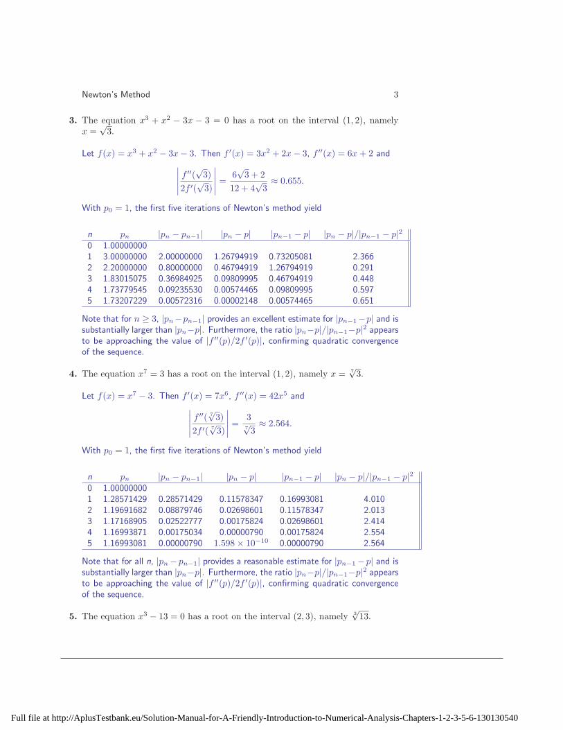
Newton’s Method 3
3. The equation x3 + x2 − 3x − 3 = 0 has a root on the interval (1, 2), namelyx =
√3.
Let f(x) = x3 + x2 − 3x − 3. Then f ′(x) = 3x2 + 2x − 3, f ′′(x) = 6x + 2 and∣
∣
∣
∣
∣
f ′′(√
3)
2f ′(√
3)
∣
∣
∣
∣
∣
=6√
3 + 2
12 + 4√
3≈ 0.655.
With p0 = 1, the first five iterations of Newton’s method yield
n pn |pn − pn−1| |pn − p| |pn−1 − p| |pn − p|/|pn−1 − p|20 1.000000001 3.00000000 2.00000000 1.26794919 0.73205081 2.3662 2.20000000 0.80000000 0.46794919 1.26794919 0.2913 1.83015075 0.36984925 0.09809995 0.46794919 0.4484 1.73779545 0.09235530 0.00574465 0.09809995 0.5975 1.73207229 0.00572316 0.00002148 0.00574465 0.651
Note that for n ≥ 3, |pn−pn−1| provides an excellent estimate for |pn−1−p| and issubstantially larger than |pn−p|. Furthermore, the ratio |pn−p|/|pn−1−p|2 appearsto be approaching the value of |f ′′(p)/2f ′(p)|, confirming quadratic convergenceof the sequence.
4. The equation x7 = 3 has a root on the interval (1, 2), namely x = 7√
3.
Let f(x) = x7 − 3. Then f ′(x) = 7x6, f ′′(x) = 42x5 and∣
∣
∣
∣
∣
f ′′( 7√
3)
2f ′( 7√
3)
∣
∣
∣
∣
∣
=37√
3≈ 2.564.
With p0 = 1, the first five iterations of Newton’s method yield
n pn |pn − pn−1| |pn − p| |pn−1 − p| |pn − p|/|pn−1 − p|20 1.000000001 1.28571429 0.28571429 0.11578347 0.16993081 4.0102 1.19691682 0.08879746 0.02698601 0.11578347 2.0133 1.17168905 0.02522777 0.00175824 0.02698601 2.4144 1.16993871 0.00175034 0.00000790 0.00175824 2.5545 1.16993081 0.00000790 1.598 × 10⁻¹⁰ 0.00000790 2.564
Note that for all n, |pn − pn−1| provides a reasonable estimate for |pn−1 − p| and issubstantially larger than |pn−p|. Furthermore, the ratio |pn−p|/|pn−1−p|2 appearsto be approaching the value of |f ′′(p)/2f ′(p)|, confirming quadratic convergenceof the sequence.
5. The equation x3 − 13 = 0 has a root on the interval (2, 3), namely 3√
13.
Full file at http://AplusTestbank.eu/Solution-Manual-for-A-Friendly-Introduction-to-Numerical-Analysis-Chapters-1-2-3-5-6-130130540
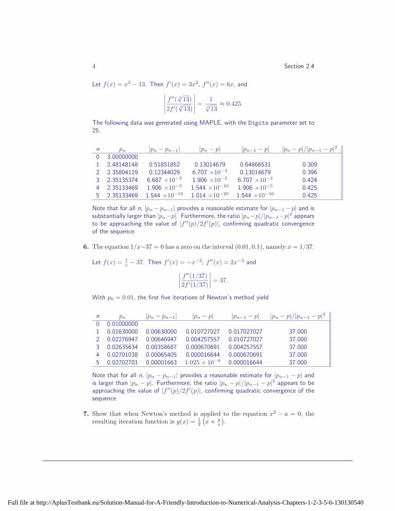
4 Section 2.4
Let f(x) = x3 − 13. Then f ′(x) = 3x2, f ′′(x) = 6x, and
∣
∣
∣
∣
∣
f ′′( 3√
13)
2f ′( 3√
13)
∣
∣
∣
∣
∣
=1
3√
13≈ 0.425.
The following data was generated using MAPLE, with the Digits parameter set to25.
n pn |pn − pn−1| |pn − p| |pn−1 − p| |pn − p|/|pn−1 − p|20 3.000000001 2.48148148 0.51851852 0.13014679 0.64866531 0.3092 2.35804119 0.12344029 6.707 ×10⁻³ 0.13014679 0.3963 2.35135374 6.687 ×10⁻³ 1.906 ×10⁻⁵ 6.707 ×10⁻³ 0.4244 2.35133469 1.906 ×10⁻⁵ 1.544 ×10⁻¹⁰ 1.906 ×10⁻⁵ 0.4255 2.35133469 1.544 ×10⁻¹⁰ 1.014 ×10⁻²⁰ 1.544 ×10⁻¹⁰ 0.425
Note that for all n, |pn − pn−1| provides a reasonable estimate for |pn−1 − p| and issubstantially larger than |pn−p|. Furthermore, the ratio |pn−p|/|pn−1−p|2 appearsto be approaching the value of |f ′′(p)/2f ′(p)|, confirming quadratic convergenceof the sequence.
6. The equation 1/x−37 = 0 has a zero on the interval (0.01, 0.1), namely x = 1/37.
Let f(x) = 1
x − 37. Then f ′(x) = −x−2, f ′′(x) = 2x−3 and
∣
∣
∣
∣
f ′′(1/37)
2f ′(1/37)
∣
∣
∣
∣
= 37.
With p0 = 0.01, the first five iterations of Newton’s method yield
n pn |pn − pn−1| |pn − p| |pn−1 − p| |pn − p|/|pn−1 − p|20 0.010000001 0.01630000 0.00630000 0.010727027 0.017027027 37.0002 0.02276947 0.00646947 0.004257557 0.010727027 37.0003 0.02635634 0.00358687 0.000670691 0.004257557 37.0004 0.02701038 0.00065405 0.000016644 0.000670691 37.0005 0.02702701 0.00001663 1.025 × 10⁻⁸ 0.000016644 37.000
Note that for all n, |pn − pn−1| provides a reasonable estimate for |pn−1 − p| andis larger than |pn − p|. Furthermore, the ratio |pn − p|/|pn−1 − p|2 appears to beapproaching the value of |f ′′(p)/2f ′(p)|, confirming quadratic convergence of thesequence.
7. Show that when Newton’s method is applied to the equation x2 − a = 0, theresulting iteration function is g(x) = 1
2
(
x + ax
)
.
Full file at http://AplusTestbank.eu/Solution-Manual-for-A-Friendly-Introduction-to-Numerical-Analysis-Chapters-1-2-3-5-6-130130540

Newton’s Method 5
Let f(x) = x2 − a. Then f ′(x) = 2x and the Newton method iteration function is
g(x) = x − f(x)
f ′(x)
= x − x2 − a
2x
=x2 + a
2x=
1
2
(
x +a
x
)
.
8. Show that when Newton’s method is applied to the equation 1/x − a = 0, theresulting iteration function is g(x) = x(2 − ax).
Let f(x) = 1
x − a. Then f ′(x) = −x−2 and the Newton method iteration functionis
g(x) = x − f(x)
f ′(x)
= x −1
x − a
−x−2
= x + x − ax2 = x(2 − ax).
9. The function f(x) = sinx has a zero on the interval (3, 4), namely x = π.Perform three iterations of Newton’s method to approximate this zero, usingp0 = 4. Determine the absolute error in each of the computed approximations.What is the apparent order of convergence? What explanation can you providefor this behavior? (NOTE: If you have access to MAPLE, perform five iterationswith the Digits parameter set to at least 100.)
Let f(x) = sinx and p0 = 4. Using MAPLE, with the Digits parameter set to100, Newton’s method yields
n |pn − p| |pn − p|/|pn−1 − p|31 2.994 ×10⁻¹
2 9.280 ×10⁻³ 0.345773 2.664 ×10⁻⁷ 0.333344 6.304 ×10⁻²¹ 0.333445 8.351 ×10−62 0.33334
Because the ratio in the third column of the table appears to be approaching aconstant, convergence is of order three. The order of convergence for this specificproblem is better than the expected quadratic convergence for Newton’s methodbecause f ′′(π) = − sin π = 0; thus,
limn→∞
|en||en−1|2
=f ′′(π)
2f ′(π)= 0,
Full file at http://AplusTestbank.eu/Solution-Manual-for-A-Friendly-Introduction-to-Numerical-Analysis-Chapters-1-2-3-5-6-130130540

6 Section 2.4
which implies that convergence is better than quadratic.
10. (a) Verify that the equation x4−18x2+45 = 0 has a root on the interval (1, 2).Next, perform three iterations of Newton’s method, with p0 = 1. Giventhat the exact value of the root is x =
√3, compute the absolute error in the
approximations just obtained. What is the apparent order of convergence?What explanation can you provide for this behavior? (NOTE: If you haveaccess to MAPLE, perform five iterations with the Digits parameter setto at least 100.)
(b) Verify that the equation x4 − 18x2 + 45 = 0 also has a root on the interval(3, 4). Perform five iterations of Newton’s method, and compute the abso-lute error in each approximation. The exact value of the root is x =
√15.
What is the apparent order of convergence in this case?
(c) What explanation can you provide for the different convergence behaviorbetween parts (a) and (b)?
(a) Let f(x) = x4 − 18x2 + 45. Then f(1) = 28 > 0 and f(2) = −11 < 0,so the Intermediate Value Theorem guarantees the existence of a root on theinterval (1, 2). With p0 = 1 and using MAPLE, with the Digits parameterset to 100, Newton’s method yields
n |pn − p| |pn − p|/|pn−1 − p|31 1.429 ×10⁻¹
2 1.014 ×10⁻³ 0.347303 3.480 ×10⁻¹⁰ 0.333264 1.404 ×10⁻²⁹ 0.333335 9.229 ×10−88 0.33333
Because the ratio in the third column of the table appears to be approaching aconstant, convergence is of order three. The order of convergence for this spe-cific problem is better than the expected quadratic convergence for Newton’smethod because f ′′(
√3) = 0; thus,
limn→∞
|en||en−1|2
=f ′′(
√3)
2f ′(√
3)= 0,
which implies that convergence is better than quadratic.
(b) Let f(x) = x4 − 18x2 + 45. Then f(3) = −36 < 0 and f(4) = 13 > 0,so the Intermediate Value Theorem guarantees the existence of a root on theinterval (3, 4). With p0 = 3.5, the following table summarizes the results offive iterations of Newton’s method.
n pn |pn − p| |pn − p|/|pn−1 − p|21 4.0590659341 1.861 × 10⁻¹
2 3.8951971117 2.221 × 10⁻² 0.6415213 3.8733563066 3.730 × 10⁻⁴ 0.7558204 3.8729834539 1.077 × 10⁻⁷ 0.7742745 3.8729833462 8.985 × 10⁻¹⁵ 0.774601
Full file at http://AplusTestbank.eu/Solution-Manual-for-A-Friendly-Introduction-to-Numerical-Analysis-Chapters-1-2-3-5-6-130130540
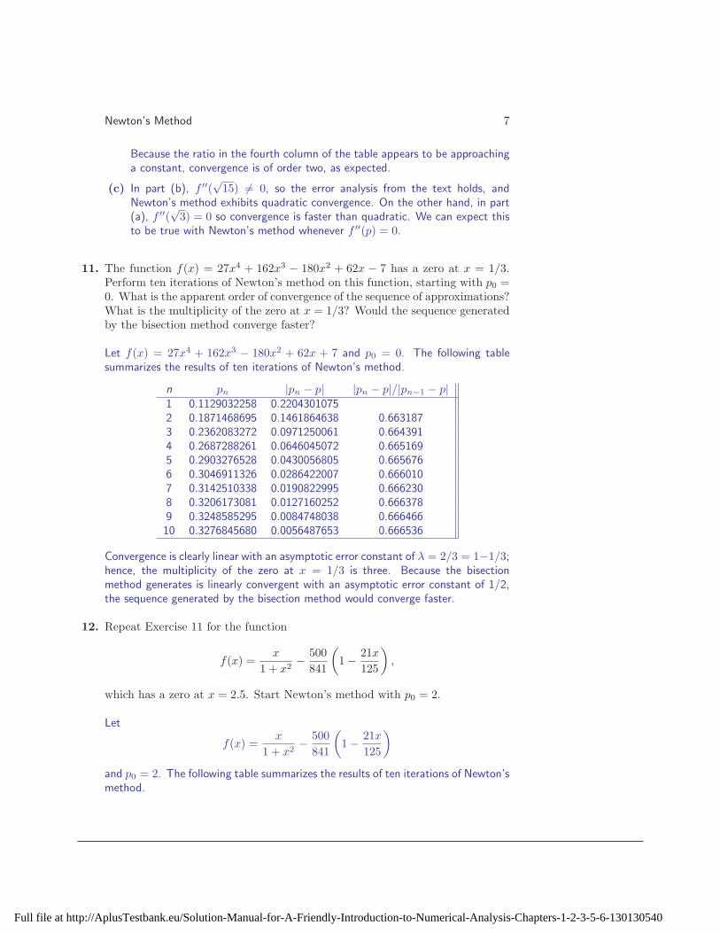
Newton’s Method 7
Because the ratio in the fourth column of the table appears to be approachinga constant, convergence is of order two, as expected.
(c) In part (b), f ′′(√
15) 6= 0, so the error analysis from the text holds, andNewton’s method exhibits quadratic convergence. On the other hand, in part(a), f ′′(
√3) = 0 so convergence is faster than quadratic. We can expect this
to be true with Newton’s method whenever f ′′(p) = 0.
11. The function f(x) = 27x4 + 162x3 − 180x2 + 62x − 7 has a zero at x = 1/3.Perform ten iterations of Newton’s method on this function, starting with p0 =0. What is the apparent order of convergence of the sequence of approximations?What is the multiplicity of the zero at x = 1/3? Would the sequence generatedby the bisection method converge faster?
Let f(x) = 27x4 + 162x3 − 180x2 + 62x + 7 and p0 = 0. The following tablesummarizes the results of ten iterations of Newton’s method.
n pn |pn − p| |pn − p|/|pn−1 − p|1 0.1129032258 0.22043010752 0.1871468695 0.1461864638 0.6631873 0.2362083272 0.0971250061 0.6643914 0.2687288261 0.0646045072 0.6651695 0.2903276528 0.0430056805 0.6656766 0.3046911326 0.0286422007 0.6660107 0.3142510338 0.0190822995 0.6662308 0.3206173081 0.0127160252 0.6663789 0.3248585295 0.0084748038 0.66646610 0.3276845680 0.0056487653 0.666536
Convergence is clearly linear with an asymptotic error constant of λ = 2/3 = 1−1/3;hence, the multiplicity of the zero at x = 1/3 is three. Because the bisectionmethod generates is linearly convergent with an asymptotic error constant of 1/2,the sequence generated by the bisection method would converge faster.
12. Repeat Exercise 11 for the function
f(x) =x
1 + x2− 500
841
(
1 − 21x
125
)
,
which has a zero at x = 2.5. Start Newton’s method with p0 = 2.
Let
f(x) =x
1 + x2− 500
841
(
1 − 21x
125
)
and p0 = 2. The following table summarizes the results of ten iterations of Newton’smethod.
Full file at http://AplusTestbank.eu/Solution-Manual-for-A-Friendly-Introduction-to-Numerical-Analysis-Chapters-1-2-3-5-6-130130540

8 Section 2.4
n pn |pn − p| |pn − p|/|pn−1 − p|1 2.2600472810 0.23995271902 2.3803798070 0.1196201930 0.4985163 2.4401402930 0.0598597070 0.5004154 2.4700436310 0.0299563690 0.5004435 2.4850136160 0.0149863840 0.5002746 2.4925046410 0.0074953590 0.5001457 2.4962520120 0.0037479880 0.5000418 2.4981261390 0.0018738610 0.4999659 2.4990646340 0.0009353660 0.49916510 2.4995334410 0.0004665590 0.498798
Convergence is clearly linear with an asymptotic error constant of λ = 1/2 = 1−1/2;hence, the multiplicity of the zero at x = 2.5 is two. Here, there is no comparisonwith the bisection method because the bisection method cannot be used to locatea root of even multiplicity.
13. The function f(x) = x3 + 2x2 − 3x − 1 has a zero on the interval (−1, 0).Approximate this zero to within an absolute tolerance of 5× 10⁻⁵.
Let f(x) = x3 + 2x2 − 3x − 1. With an initial approximation of p0 = 0 and aconvergence tolerance of 5 × 10⁻⁵, Newton’s method yields
n pn
1 −0.33333333332 −0.28703703703 −0.28646216164 −0.2864620650
Thus, the zero of f(x) = x3 +2x2−3x−1 on the interval (−1, 0) is approximatelyx = −0.286462.
14. For each of the functions given below, use Newton’s method to approximate allreal roots. Use an absolute tolerance of 10−6 as a stopping condition.
(a) f(x) = ex + x2 − x − 4
(b) f(x) = x3 − x2 − 10x + 7
(c) f(x) = 1.05 − 1.04x + lnx
(a) Let f(x) = ex +x2 −x− 4. Observe that the equation ex +x2 −x− 4 = 0 isequivalent to the equation ex = −x2 + x + 4. The figure below displays thegraphs of y = ex and y = −x2 + x + 4.
Full file at http://AplusTestbank.eu/Solution-Manual-for-A-Friendly-Introduction-to-Numerical-Analysis-Chapters-1-2-3-5-6-130130540
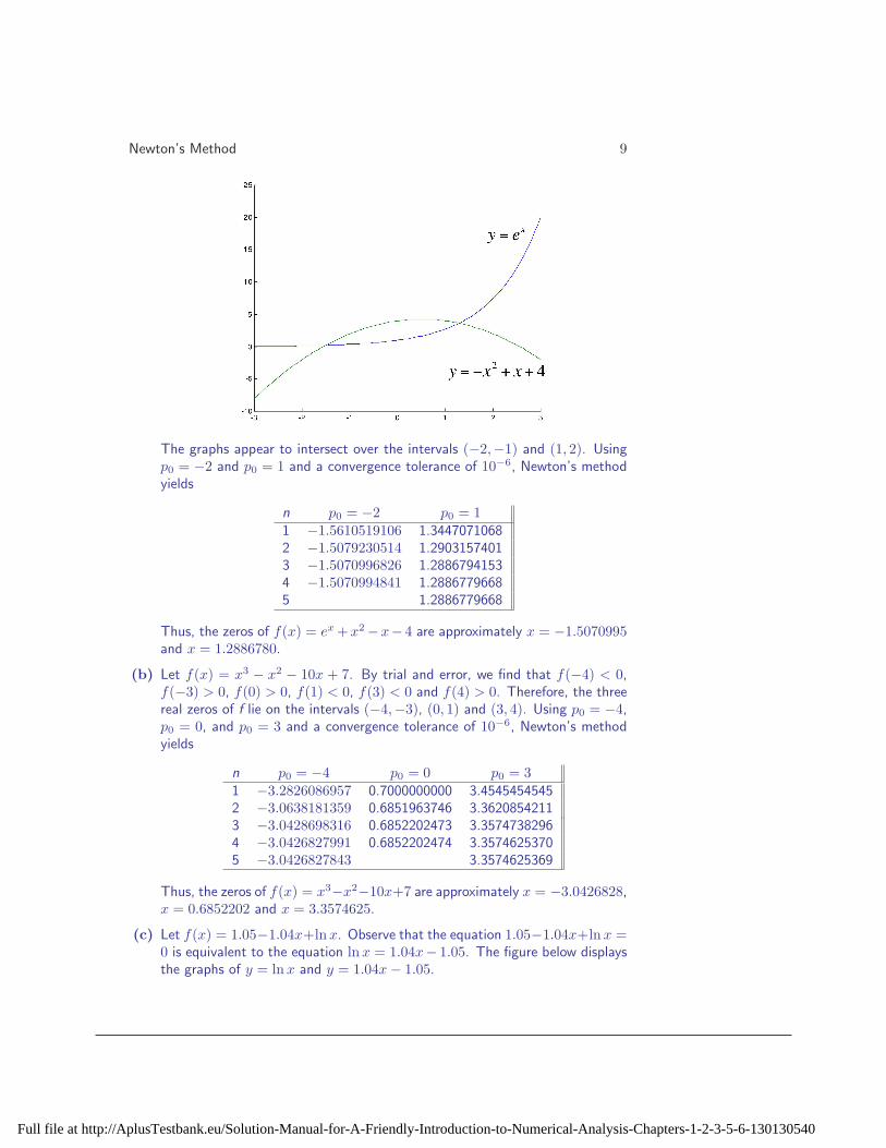
Newton’s Method 9
The graphs appear to intersect over the intervals (−2,−1) and (1, 2). Usingp0 = −2 and p0 = 1 and a convergence tolerance of 10−6, Newton’s methodyields
n p0 = −2 p0 = 11 −1.5610519106 1.34470710682 −1.5079230514 1.29031574013 −1.5070996826 1.28867941534 −1.5070994841 1.28867796685 1.2886779668
Thus, the zeros of f(x) = ex +x2 −x− 4 are approximately x = −1.5070995and x = 1.2886780.
(b) Let f(x) = x3 − x2 − 10x + 7. By trial and error, we find that f(−4) < 0,f(−3) > 0, f(0) > 0, f(1) < 0, f(3) < 0 and f(4) > 0. Therefore, the threereal zeros of f lie on the intervals (−4,−3), (0, 1) and (3, 4). Using p0 = −4,p0 = 0, and p0 = 3 and a convergence tolerance of 10−6, Newton’s methodyields
n p0 = −4 p0 = 0 p0 = 31 −3.2826086957 0.7000000000 3.45454545452 −3.0638181359 0.6851963746 3.36208542113 −3.0428698316 0.6852202473 3.35747382964 −3.0426827991 0.6852202474 3.35746253705 −3.0426827843 3.3574625369
Thus, the zeros of f(x) = x3−x2−10x+7 are approximately x = −3.0426828,x = 0.6852202 and x = 3.3574625.
(c) Let f(x) = 1.05−1.04x+ln x. Observe that the equation 1.05−1.04x+ln x =0 is equivalent to the equation lnx = 1.04x− 1.05. The figure below displaysthe graphs of y = lnx and y = 1.04x − 1.05.
Full file at http://AplusTestbank.eu/Solution-Manual-for-A-Friendly-Introduction-to-Numerical-Analysis-Chapters-1-2-3-5-6-130130540
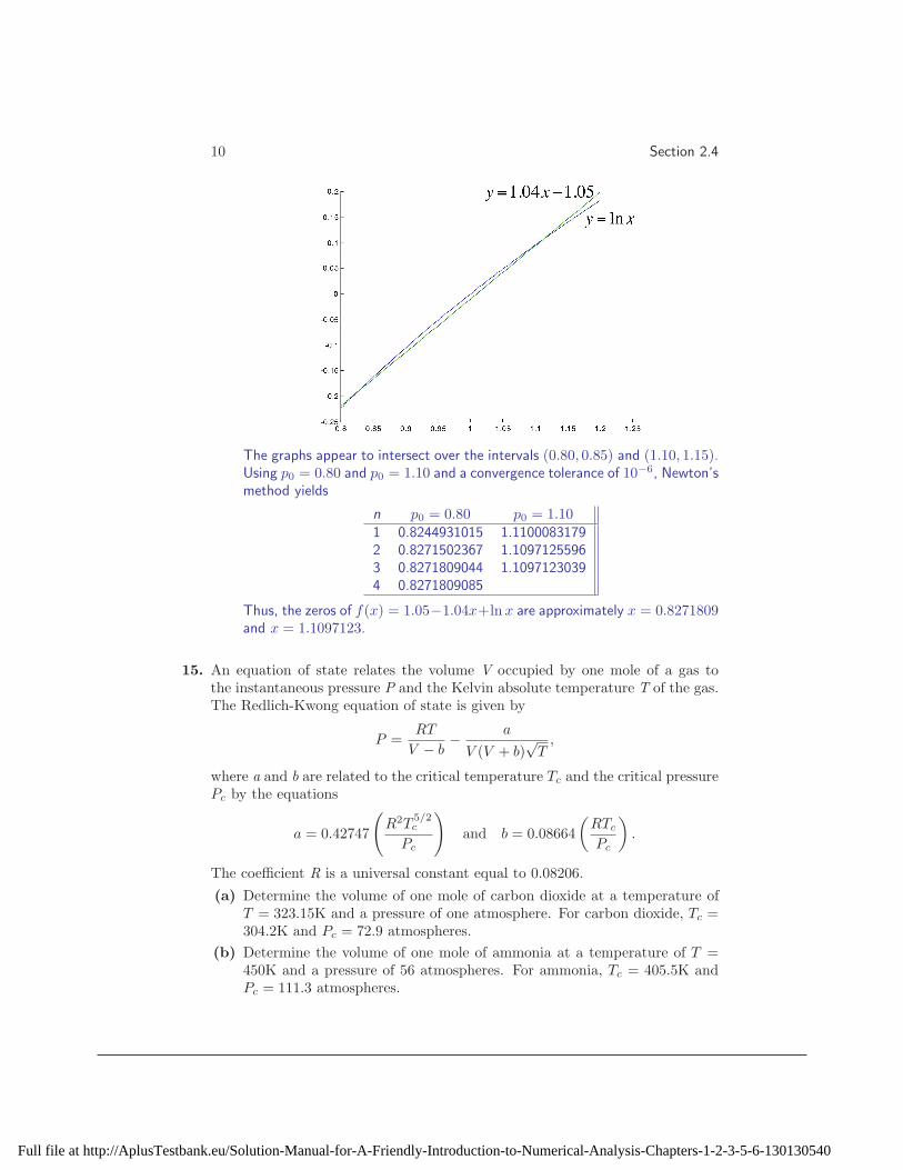
10 Section 2.4
The graphs appear to intersect over the intervals (0.80, 0.85) and (1.10, 1.15).Using p0 = 0.80 and p0 = 1.10 and a convergence tolerance of 10−6, Newton’smethod yields
n p0 = 0.80 p0 = 1.101 0.8244931015 1.11000831792 0.8271502367 1.10971255963 0.8271809044 1.10971230394 0.8271809085
Thus, the zeros of f(x) = 1.05−1.04x+ln x are approximately x = 0.8271809and x = 1.1097123.
15. An equation of state relates the volume V occupied by one mole of a gas tothe instantaneous pressure P and the Kelvin absolute temperature T of the gas.The Redlich-Kwong equation of state is given by
P =RT
V − b− a
V (V + b)√
T,
where a and b are related to the critical temperature Tc and the critical pressurePc by the equations
a = 0.42747
(
R2T5/2c
Pc
)
and b = 0.08664
(
RTc
Pc
)
.
The coefficient R is a universal constant equal to 0.08206.
(a) Determine the volume of one mole of carbon dioxide at a temperature ofT = 323.15K and a pressure of one atmosphere. For carbon dioxide, Tc =304.2K and Pc = 72.9 atmospheres.
(b) Determine the volume of one mole of ammonia at a temperature of T =450K and a pressure of 56 atmospheres. For ammonia, Tc = 405.5K andPc = 111.3 atmospheres.
Full file at http://AplusTestbank.eu/Solution-Manual-for-A-Friendly-Introduction-to-Numerical-Analysis-Chapters-1-2-3-5-6-130130540

Newton’s Method 11
Let
f(V ) =RT
V − b− a
V (V + b)√
T− P.
Then
f ′(V ) = − RT
(V − b)2+
a(2V + b)
V 2(V + b)2√
T.
(a) For carbon dioxide, Tc = 304.2 K and Pc = 72.9 atmospheres, so
a = 0.427470.082062 · 304.25/2
72.9= 63.72930208
and
b = 0.086640.08206 · 304.2
72.9= 0.029667546.
The initial approximation for the volume is taken from the ideal gas law:
V0 =nRT
P=
(1 mole)(0.08206 atm · liter/mole · K)(323.15 K)
1 atmosphere
= 26.517689 liters.
With a convergence tolerance of 5 × 10⁻⁷, Newton’s method yields
n Vn
1 26.41302946222 26.41343928853 26.4134392948
Thus, one mole of carbon dioxide at a temperature of 323.15 K and a pressureof one atmosphere occupies a volume of approximately 26.4134 liters.
(b) For ammonia, Tc = 405.5 K and Pc = 111.3 atmospheres, so
a = 0.427470.082062 · 405.55/2
111.3= 85.634487113
and
b = 0.086640.08206 · 405.5
111.3= 0.259027366.
The initial approximation for the volume is taken from the ideal gas law:
V0 =nRT
P=
(1 mole)(0.08206 atm · liter/mole · K)(450 K)
56 atmosphere
= 0.659410714 liters.
With a convergence tolerance of 5 × 10⁻⁷, Newton’s method yields
n Vn
1 0.55787598822 0.56959323803 0.56980363854 0.5698037041
Full file at http://AplusTestbank.eu/Solution-Manual-for-A-Friendly-Introduction-to-Numerical-Analysis-Chapters-1-2-3-5-6-130130540

12 Section 2.4
Thus, one mole of ammonia at a temperature of 450 K and a pressure of 56atmospheres occupies a volume of approximately 0.5698 liters.
16. In determining the minimum cushion pressure needed to break a given thicknessof ice using an air cushion vehicle, Muller (“Ice Breaking with an Air CushionVehicle,” in Mathematical Modeling: Classroom Notes in Applied Mathematics,M.S. Klamkin, editor, SIAM, 1987) derived the equation
p3(1 − β2) +
(
0.4hβ2 − σh2
r2
)
p2 +σ2h4
3r4p −
(
σh2
3r2
)3
= 0,
where p denotes the cushion pressure, h the thickness of the ice field, r the sizeof the air cushion, σ the tensile strength of the ice, and β is related to the widthof the ice wedge. Take β = 0.5, r = 40 feet and σ = 150 pounds per square inch(psi). Determine p for h = 0.6, 1.2, 1.8, 2.4, 3.0, 3.6 and 4.2 feet.
Let
f(p) = (1 − β2)p3 +
(
0.4hβ2 − σh2
r2
)
p2 +σ2h4
3r4p −
(
σh2
3r2
)3
.
Then
f ′(p) = 3(1 − β2)p2 + 2
(
0.4hβ2 − σh2
r2
)
p +σ2h4
3r4.
With a starting approximation of p0 = 0 and a convergence tolerance of 5 × 10⁻⁷,Newton’s method yields
h (feet) 0.6 1.2 1.8 2.4 3.0 3.6 4.2p (psi) 0.003050 0.015138 0.038278 0.073664 0.122199 0.184644 0.261681
17. A frame structure is composed of two vertical columns and one horizontal beam,as shown below. The vertical columns are of length L and have modulus of elas-ticity E and moment of inertia I. The horizontal beam connecting the tops ofthe columns is of length L1 with modulus of elasticity E and moment of inertiaI1. The structure is pinned at the bottom and free to displace laterally at thetop. The buckling load, P, for the structure is given by
P PP = (kL)2
EI
L2,
where kL is the smallest positive solution of
kL tan kL = 6I1L
IL1
.
Suppose E = 30 × 106 lb/in2, I = 15.2 in4,L = 144 in, I1 = 9.7 in4 and L1 = 120 in.Determine the buckling load of the structure.
Full file at http://AplusTestbank.eu/Solution-Manual-for-A-Friendly-Introduction-to-Numerical-Analysis-Chapters-1-2-3-5-6-130130540

Newton’s Method 13
Let x = kL and define the function
f(x) = x tanx − 6I1L
IL1
.
Then f ′(x) = x sec2 x + tanx. With an initial approximation of x0 = 1.5 and aconvergence tolerance of 5 × 10⁻⁷, Newton’s method yields
n xn
1 1.44724869882 1.37894081513 1.32080206574 1.29812924815 1.29591527906 1.29589738067 1.2958973794
Thus, kL ≈ 1.295897, and the buckling load of the structure is approximately
P = (1.295897)230 × 106 · 15.2
1442= 36.930 × 10³ lb.
Full file at http://AplusTestbank.eu/Solution-Manual-for-A-Friendly-Introduction-to-Numerical-Analysis-Chapters-1-2-3-5-6-130130540
Secant Method 1
2.5 Secant Method
1. Each of the following equations has a root on the interval (0, 1). Perform thesecant method to determine p4, the fourth approximation to the location of theroot.
(a) ln(1 + x) − cos x = 0 (b) x5 + 2x − 1 = 0(c) e−x − x = 0 (d) cos x − x = 0
(a) Let f(x) = ln(1 +x)− cos x. With p0 = 0 and p1 = 1, three iterations of thesecant method yield
p2 = p1 − (ln(1 + p1) − cos p1)p1 − p0
(ln(1 + p1) − cos p1) − (ln(1 + p0) − cos p0)
= 0.8674193918;
p3 = p2 − (ln(1 + p2) − cos p2)p2 − p1
(ln(1 + p2) − cos p2) − (ln(1 + p1) − cos p1)
= 0.8842599009; and
p4 = p3 − (ln(1 + p3) − cos p3)p3 − p2
(ln(1 + p3) − cos p3) − (ln(1 + p2) − cos p2)
= 0.8845112004
(b) Let f(x) = x5 + 2x − 1. With p0 = 0 and p1 = 1, three iterations of thesecant method yield
p2 = p1 − (p51 + 2p1 − 1)
p1 − p0
(p51 + 2p1 − 1) − (p5
0 + 2p0 − 1)
= 0.3333333333;
p3 = p2 − (p52 + 2p2 − 1)
p2 − p1
(p52 + 2p2 − 1) − (p5
1 + 2p1 − 1)
= 0.4275618375; and
p4 = p3 − (p53 + 2p3 − 1)
p3 − p2
(p53 + 2p3 − 1) − (p5
2 + 2p2 − 1)
= 0.4895113751
(c) Let f(x) = e−x − x. With p0 = 0 and p1 = 1, three iterations of the secantmethod yield
p2 = p1 − (e−p1 − p1)p1 − p0
(e−p1 − p1) − (e−p0 − p0)
Full file at http://AplusTestbank.eu/Solution-Manual-for-A-Friendly-Introduction-to-Numerical-Analysis-Chapters-1-2-3-5-6-130130540
2 Section 2.5
= 0.6126998368;
p3 = p2 − (e−p2 − p2)p2 − p1
(e−p2 − p2) − (e−p1 − p1)
= 0.5638383892; and
p4 = p3 − (e−p3 − p3)p3 − p2
(e−p3 − p3) − (e−p2 − p2)
= 0.5671703584
(d) Let f(x) = cos x − x. With p0 = 0 and p1 = 1, three iterations of the secantmethod yield
p2 = p1 − (cos p1 − p1)p1 − p0
(cos p1 − p1) − (cos p0 − p0)
= 0.6850733573;
p3 = p2 − (cos p2 − p2)p2 − p1
(cos p2 − p2) − (cos p1 − p1)
= 0.7362989976; and
p4 = p3 − (cos p3 − p3)p3 − p2
(cos p3 − p3) − (cos p2 − p2)
= 0.7391193619
2. Construct an algorithm for the secant method.
The stopping condition in STEP 3 is justified by the superlinear convergence (α ≈1.618) of the secant method.
GIVEN: function whose zero is to be located, f
starting approximations x0 and x1
convergence parameter ǫmaximum number of iterations Nmax
STEP 1: for iter from 1 to Nmax
STEP 2: compute x2 = x1 − f(x1)(x1 − x0)/(f(x1) − f(x0))STEP 3: if |x2 − x1| < ǫ, OUTPUT x2
STEP 4: copy the value of x1 to x0
copy the value of x2 to x1
endOUTPUT: “maximum number of iterations has been exceeded”
3. Show that the equation for the secant method can be rewritten as
pn+1 =f(pn)pn−1 − f(pn−1)pn
f(pn) − f(pn−1).
Full file at http://AplusTestbank.eu/Solution-Manual-for-A-Friendly-Introduction-to-Numerical-Analysis-Chapters-1-2-3-5-6-130130540

Secant Method 3
Explain why this formula is inferior to the one used in the text.
We proceed as follows:
pn+1 = pn − f(pn)pn − pn−1
f(pn) − f(pn−1)
=pnf(pn) − pnf(pn−1) − pnf(pn) + pn−1f(pn)
f(pn) − f(pn−1)
=f(pn)pn−1 − f(pn−1)pn
f(pn) − f(pn−1).
Note that both formulas for calculating pn+1 have the potential for cancellationerror. In the formula
pn+1 = pn − f(pn)pn − pn−1
f(pn) − f(pn−1),
cancellation error will primarily influence the second term, which is essentially justa correction to pn. This can limit the overall effect of roundoff error on pn+1. Inthe formula
pn+1 =f(pn)pn−1 − f(pn−1)pn
f(pn) − f(pn−1),
however, cancellation error influences the entire calculation. Thus, the latter formulais inferior to the former because it is more susceptible to roundoff error.
4. Fill in the missing details in the derivation of the error evolution equation
pn+1 − p ≈ (pn − p)(pn−1 − p)f ′′(p)
2f ′(p) + f ′′(p)(pn + pn−1 − 2p).
First subtract the true root, p, from both sides of the recurrence formula for pn−1,yielding
pn+1 − p = pn − p − f(pn)pn − pn−1
f(pn) − f(pn−1). (1)
Next, approximate the function values f(pn−1) and f(pn) by the second degreeTaylor polynomials
f(pn−1) ≈ f ′(p)(pn−1 − p) +f ′′(p)
2(pn−1 − p)2, (2)
f(pn) ≈ f ′(p)(pn − p) +f ′′(p)
2(pn − p)2, (3)
The term f(pn) − f(pn−1) is then approximately
f(pn) − f(pn−1) ≈ f ′(p)(pn − pn−1) +f ′′(p)
2
[
(pn − p)2 − (pn−1 − p)2]
= (pn − pn−1)
[
f ′(p) +f ′′(p)
2(pn + pn−1 − 2p)
]
. (4)
Full file at http://AplusTestbank.eu/Solution-Manual-for-A-Friendly-Introduction-to-Numerical-Analysis-Chapters-1-2-3-5-6-130130540

4 Section 2.5
Substituting (2), (3) and (4) into (1), factoring the term pn − p and dividing outthe term pn − pn−1 yields
pn+1 − p ≈ (pn − p)
[
1 − f ′(p) + f ′′(p)2 (pn − p)
f ′(p) + f ′′(p)2 (pn + pn−1 − 2p)
]
≈ (pn − p)(pn−1 − p)f ′′(p)
2f ′(p) + f ′′(p)(pn + pn−1 − 2p).
In Exercises 5 - 8, an equation, an interval on which the equation has a root,and the exact value of the root are specified.(a) Perform seven (7) iterations of the secant method.(b) For n ≥ 2, compare |pn − pn−1| with |pn−1 − p| and |pn − p|.(c) For n ≥ 2, compute the ratio |pn − p|/|pn−1 − p|1.618 and show that this
value approaches (|f ′′(p)/2f ′(p)|)0.618.
5. The equation x3 + x2 − 3x − 3 = 0 has a root on the interval (1, 2), namelyx =
√3.
Let f(x) = x3 + x2 − 3x − 3. Then f ′(x) = 3x2 + 2x − 3, f ′′(x) = 6x + 2 and
(∣
∣
∣
∣
∣
f ′′(√
3)
2f ′(√
3)
∣
∣
∣
∣
∣
)0.618
=
(
6√
3 + 2
12 + 4√
3
)0.618
≈ 0.770.
With p0 = 1 and p1 = 2, the first seven iterations of the secant method yield
n pn |pn − pn−1| |pn − p| |pn−1 − p| |pn − p|/|pn−1 − p|1.618
0 1.000000001 2.000000002 1.57142857 0.42857143 1.606 ×10⁻¹ 2.679 ×10⁻¹ 1.3533 1.70541082 0.13398225 2.664 ×10⁻² 1.606 ×10⁻¹ 0.5134 1.73513577 0.02972495 3.085 ×10⁻³ 2.664 ×10⁻² 1.0885 1.73199637 0.00313940 5.444 ×10⁻⁵ 3.085 ×10⁻³ 0.6286 1.73205070 0.00005433 1.098 ×10⁻⁷ 5.444 ×10⁻⁵ 0.8717 1.73205081 0.00000011 3.193 ×10⁻¹² 1.098 ×10⁻⁷ 0.713
Note that for n ≥ 3, |pn − pn−1| provides an excellent estimate for |pn−1 − p| andis substantially larger than |pn − p|. Furthermore, the ratio |pn − p|/|pn−1 − p|1.618
appears to be settling toward the value of (|f ′′(p)/2f ′(p)|)0.618, confirming thesequence converges of order α ≈ 1.618.
6. The equation x7 = 3 has a root on the interval (1, 2), namely x = 7√
3.
Full file at http://AplusTestbank.eu/Solution-Manual-for-A-Friendly-Introduction-to-Numerical-Analysis-Chapters-1-2-3-5-6-130130540
Secant Method 5
Let f(x) = x7 − 3. Then f ′(x) = 7x6, f ′′(x) = 42x5 and
(∣
∣
∣
∣
∣
f ′′( 7√
3)
2f ′( 7√
3)
∣
∣
∣
∣
∣
)0.618
=
(
37√
3
)0.618
≈ 1.790.
With p0 = 1 and p1 = 2, the first seven iterations of the secant method yield
n pn |pn − pn−1| |pn − p| |pn−1 − p| |pn − p|/|pn−1 − p|1.618
0 1.000000001 2.000000002 1.01574803 0.98425197 1.542 × 10⁻¹ 8.301 × 10⁻¹ 0.2083 1.03036560 0.01461756 1.396 × 10⁻¹ 1.542 × 10⁻¹ 2.8744 1.25047859 0.22011299 8.055 × 10⁻² 1.396 × 10⁻¹ 1.9495 1.13998478 0.11049380 2.995 × 10⁻² 8.055 × 10⁻² 1.7636 1.16412646 0.02414168 5.804 × 10⁻³ 2.995 × 10⁻² 1.6947 1.17039516 0.00626869 4.643 × 10⁻⁴ 5.804 × 10⁻³ 1.928
Note that for n ≥ 3, |pn − pn−1| provides an excellent estimate for |pn−1 − p| andis substantially larger than |pn − p|. Furthermore, the ratio |pn − p|/|pn−1 − p|1.618
appears to be settling toward the value of (|f ′′(p)/2f ′(p)|)0.618, confirming thesequence converges of order α ≈ 1.618.
7. The equation x3 − 13 = 0 has a root on the interval (2, 3), namely 3√
13.
Let f(x) = x3 − 13. Then f ′(x) = 3x2, f ′′(x) = 6x, and
(∣
∣
∣
∣
∣
f ′′( 3√
13)
2f ′( 3√
13)
∣
∣
∣
∣
∣
)0.618
=
(
13√
13
)0.618
≈ 0.589.
With p0 = 2 and p1 = 3, the first seven iterations of the secant method yield
n pn |pn − pn−1| |pn − p| |pn−1 − p| |pn − p|/|pn−1 − p|1.618
0 2.000000001 3.000000002 2.26315789 0.73684211 8.818 ×10⁻² 6.487 ×10⁻¹ 0.1783 2.33050735 0.06734946 2.083 ×10⁻² 8.818 ×10⁻² 1.0594 2.35214053 0.02163318 8.058 ×10⁻⁴ 2.083 ×10⁻² 0.4235 2.35132751 0.00081302 7.179 ×10⁻⁶ 8.058 ×10⁻⁴ 0.7276 2.35133469 0.00000718 2.460 ×10⁻⁹ 7.179 ×10⁻⁶ 0.5177 2.35133469 2.460 ×10⁻⁹ 7.550 ×10⁻¹⁵ 2.460 ×10⁻⁹ 0.642
Note that for n ≥ 3, |pn − pn−1| provides an excellent estimate for |pn−1 − p| andis substantially larger than |pn − p|. Furthermore, the ratio |pn − p|/|pn−1 − p|1.618
appears to be settling toward the value of (|f ′′(p)/2f ′(p)|)0.618, confirming thesequence converges of order α ≈ 1.618.
Full file at http://AplusTestbank.eu/Solution-Manual-for-A-Friendly-Introduction-to-Numerical-Analysis-Chapters-1-2-3-5-6-130130540

6 Section 2.5
8. The equation 1/x−37 = 0 has a zero on the interval (0.01, 0.1), namely x = 1/37.
Let f(x) = 1x− 37. Then f ′(x) = −x−2, f ′′(x) = 2x−3 and
(∣
∣
∣
∣
f ′′(1/37)
2f ′(1/37)
∣
∣
∣
∣
)0.618
= 370.618 ≈ 9.314.
With p0 = 0.01 and p1 = 0.02, the first seven iterations of the secant method yield
n pn |pn − pn−1| |pn − p| |pn−1 − p| |pn − p|/|pn−1 − p|1.618
0 0.010000001 0.020000002 0.02260000 0.00260000 4.427 × 10⁻³ 7.027 × 10⁻³ 13.4913 0.02587600 0.00327600 1.151 × 10⁻³ 4.427 × 10⁻³ 7.4084 0.02683849 0.00096249 1.885 × 10⁻⁴ 1.151 × 10⁻³ 10.7295 0.02701900 0.00018051 8.029 × 10⁻⁶ 1.885 × 10⁻⁴ 8.5336 0.02702697 0.00000797 5.601 × 10⁻⁸ 8.029 × 10⁻⁶ 9.8297 0.02702703 0.00000006 1.664 × 10⁻¹¹ 5.601 × 10⁻⁸ 9.004
Note that for n ≥ 3, |pn − pn−1| provides an excellent estimate for |pn−1 − p| andis substantially larger than |pn − p|. Furthermore, the ratio |pn − p|/|pn−1 − p|1.618
appears to be settling toward the value of (|f ′′(p)/2f ′(p)|)0.618, confirming thesequence converges of order α ≈ 1.618.
9. The function f(x) = sinx has a zero on the interval (3, 4), namely x = π.Perform five iterations of the secant method to approximate this zero, usingp0 = 3 and p1 = 4. Determine the absolute error in each of the computedapproximations. What is the apparent order of convergence? What explanationcan you provide for this behavior? (NOTE: If you have access to MAPLE,perform seven iterations with the Digits parameter set to at least 100.)
Let f(x) = sinx and take p0 = 3 and p1 = 4. Using MAPLE, with the Digits
parameter set to 100, the secant method yields
n |pn − p| |pn − p|/|pn−1 − p|20 1.416 ×10⁻¹
1 8.584 ×10⁻¹
2 1.557 ×10⁻² 0.021133 2.134 ×10⁻³ 8.800744 7.440 ×10⁻⁸ 0.016345 5.644 ×10⁻¹⁴ 10.197596 5.206 ×10⁻²⁹ 0.016347 2.764 ×10−56 10.19759
Because the ratio in the third column of the table appears to have settled into atwo-cycle, convergence appears to be of order two. The order of convergence for
Full file at http://AplusTestbank.eu/Solution-Manual-for-A-Friendly-Introduction-to-Numerical-Analysis-Chapters-1-2-3-5-6-130130540

Secant Method 7
this specific problem is better than the expected α ≈ 1.618 for the secant methodbecause f ′′(π) = − sin π = 0; thus,
limn→∞
|en||en−1|1.618
=
(
f ′′(π)
2f ′(π)
)0.618
= 0,
which implies that convergence is better than order α ≈ 1.618.
10. (a) Verify that the equation x4 − 18x2 + 45 = 0 has a root on the interval(1, 2). Next, perform five iterations of the secant method, using p0 = 1and p1 = 2. Given that the exact value of the root is x =
√3, compute the
absolute error in the approximations just obtained. What is the apparentorder of convergence? What explanation can you provide for this behavior?(NOTE: If you have access to MAPLE, perform seven iterations with theDigits parameter set to at least 100.)
(b) Verify that the equation x4 − 18x2 + 45 = 0 also has a root on the interval(3, 4). Perform seven iterations of the secant method, and compute theabsolute error in each approximation. The exact value of the root is
√15.
What is the apparent order of convergence in this case? What explanationcan you provide for the different convergence behavior between parts (a)and (b)?
(a) Let f(x) = x4 −18x2 +45. Then f(1) = 28 > 0 and f(2) = −11 < 0, so theIntermediate Value Theorem guarantees the existence of a root on the interval(1, 2). With p0 = 1, p1 = 2 and using MAPLE, with the Digits parameterset to 100, the secant method yields
n |pn − p| |pn − p|/|pn−1 − p|22 1.410 × 10⁻² 0.196423 1.681 × 10⁻⁴ 0.845044 5.493 × 10⁻⁹ 0.194495 2.585 × 10⁻¹⁷ 0.856946 1.300 × 10⁻³⁴ 0.194497 1.448 × 10−68 0.85694
Because the ratio in the third column of the table appears to have settled intoa two-cycle, convergence appears to be of order two. The order of convergencefor this specific problem is better than the expected α ≈ 1.618 for the secantmethod because f ′′(
√3) = 0; thus,
limn→∞
|en||en−1|1.618
=
(
f ′′(√
3)
2f ′(√
3)
)0.618
= 0,
which implies that convergence is better than order α ≈ 1.618.
(b) Let f(x) = x4 −18x2 +45. Then f(3) = −36 < 0 and f(4) = 13 > 0, so theIntermediate Value Theorem guarantees the existence of a root on the interval
Full file at http://AplusTestbank.eu/Solution-Manual-for-A-Friendly-Introduction-to-Numerical-Analysis-Chapters-1-2-3-5-6-130130540

8 Section 2.5
(3, 4). With p0 = 3 and p1 = 4, the following table summarizes the results ofseven iterations of the secant method.
n pn |pn − p| |pn − p|/|pn−1 − p|1.618
2 3.73469388 1.383 × 10⁻¹ 3.8973 3.85932813 1.366 × 10⁻² 0.3354 3.87458114 1.598 × 10⁻³ 1.6625 3.87296633 1.701 × 10⁻⁵ 0.5706 3.87298333 2.104 × 10⁻⁸ 1.0957 3.87298335 2.771 × 10⁻¹³ 0.731
Because the ratio in the fourth column of the table appears to be approachinga constant, convergence is of order α ≈ 1.618, as expected.
(c) In part (b), f ′′(√
15) 6= 0, so the error analysis from the text holds, and thesecant method exhibits convergence of order α ≈ 1.618. On the other hand,in part (a), f ′′(
√3) = 0 so convergence is faster. We can expect this to be
true with the secant method whenever f ′′(p) = 0.
11. It was observed that Newton’s method provides only linear convergence towardsroots of multiplicity greater than one. How does the secant method performunder such circumstances? Each of the following functions has a zero at thespecified location. Perform ten iterations of the secant method to locate thesezeros. Does the sequence generated by the secant method converge with orderα ≈ 1.618 or has the order dropped to α = 1?
(a) f(x) = x(1 − cos x) has a zero at x = 0 – use p0 = −1 and p1 = 2
(b) f(x) = 27x4 + 162x3 − 180x2 + 62x − 7 has a zero at x = 1/3
(c) f(x) = x1+x2 − 500
841
(
1 − 21x125
)
has a zero at x = 2.5
(a) Let f(x) = x(1 − cos x). With p0 = −1 and p1 = 2, ten iterations of thesecant method yield
n pn |pn − p| |pn − p|/|pn−1 − p|0 −1.000000001 2.000000002 −0.58107634 0.58107634 0.2913 −0.49699597 0.49699597 0.8554 −0.35355090 0.35355090 0.7115 −0.27156471 0.27156471 0.7686 −0.20308551 0.20308551 0.7487 −0.15362583 0.15362583 0.7568 −0.11577717 0.11577717 0.7549 −0.08741103 0.08741103 0.75510 −0.06596265 0.06596265 0.755
Because the ratio of errors in the fourth column approaches a constant, it isclear that the order of convergence has dropped to linear.
Full file at http://AplusTestbank.eu/Solution-Manual-for-A-Friendly-Introduction-to-Numerical-Analysis-Chapters-1-2-3-5-6-130130540

Secant Method 9
(b) Let f(x) = 27x4 + 162x3 − 180x2 + 62x − 7. With p0 = 0 and p1 = 1, teniterations of the secant method yield
n pn |pn − p| |pn − p|/|pn−1 − p|0 0.000000001 1.000000002 0.09859155 0.23474178 0.3523 0.13220733 0.20112601 0.8574 0.18992728 0.14340605 0.7135 0.22316577 0.11016756 0.7686 0.25096822 0.08236511 0.7487 0.27106015 0.06227318 0.7568 0.28642787 0.04690546 0.7539 0.29793792 0.03539541 0.75510 0.30663456 0.02669878 0.754
Because the ratio of errors in the fourth column approaches a constant, it isclear that the order of convergence has dropped to linear.
(c) Let
f(x) =x
1 + x2− 500
841
(
1 − 21x
125
)
.
With p0 = 2 and p1 = 3, ten iterations of the secant method yield
n pn |pn − p| |pn − p|/|pn−1 − p|0 2.000000001 3.000000002 46.00000000 43.50000000 87.0003 2.94526305 0.44526305 0.0104 2.90154959 0.40154959 0.9025 2.70634662 0.20634662 0.5146 2.63456117 0.13456117 0.6527 2.58094899 0.08094899 0.6028 2.55037793 0.05037793 0.6229 2.53099767 0.03099767 0.61510 2.51917084 0.01917084 0.618
Because the ratio of errors in the fourth column approaches a constant, it isclear that the order of convergence has dropped to linear.
12. Newton’s method approximates the zero of f(x) = x3 + 2x2 − 3x − 1 on theinterval (−3,−2) to within 9.436 × 10⁻¹¹ in 3 iterations and 6 function eval-uations. How many iterations and how many function evaluations are neededby the secant method to approximate this zero to a similar accuracy? Takep0 = −2 and p1 = −3.
To 15 decimal places, the zero of f(x) = x3 +2x2−3x−1 on the interval (−3,−2)is −2.912229178484397. With p0 = −2 and p1 = −3, the secant method yields
Full file at http://AplusTestbank.eu/Solution-Manual-for-A-Friendly-Introduction-to-Numerical-Analysis-Chapters-1-2-3-5-6-130130540
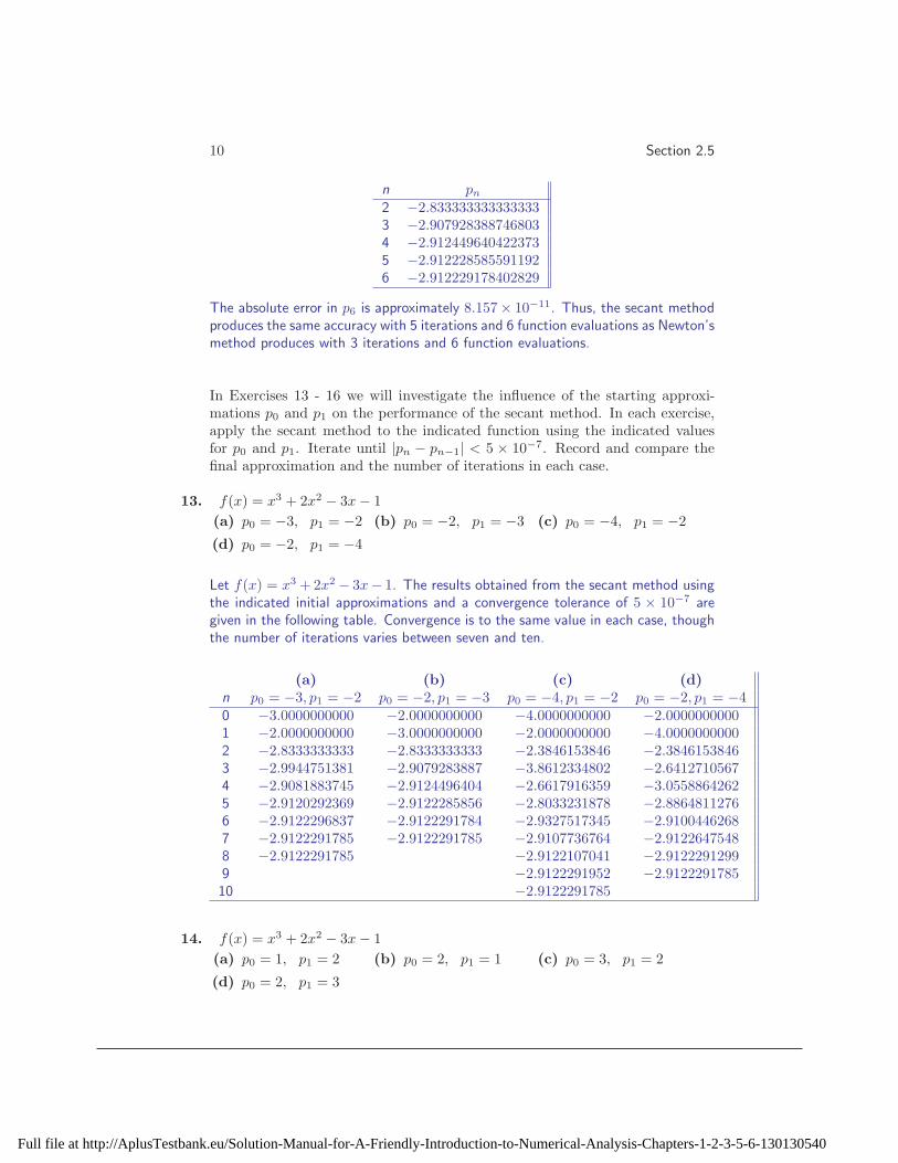
10 Section 2.5
n pn
2 −2.8333333333333333 −2.9079283887468034 −2.9124496404223735 −2.9122285855911926 −2.912229178402829
The absolute error in p6 is approximately 8.157× 10⁻¹¹. Thus, the secant methodproduces the same accuracy with 5 iterations and 6 function evaluations as Newton’smethod produces with 3 iterations and 6 function evaluations.
In Exercises 13 - 16 we will investigate the influence of the starting approxi-mations p0 and p1 on the performance of the secant method. In each exercise,apply the secant method to the indicated function using the indicated valuesfor p0 and p1. Iterate until |pn − pn−1| < 5 × 10⁻⁷. Record and compare thefinal approximation and the number of iterations in each case.
13. f(x) = x3 + 2x2 − 3x − 1
(a) p0 = −3, p1 = −2 (b) p0 = −2, p1 = −3 (c) p0 = −4, p1 = −2
(d) p0 = −2, p1 = −4
Let f(x) = x3 + 2x2 − 3x− 1. The results obtained from the secant method usingthe indicated initial approximations and a convergence tolerance of 5 × 10⁻⁷ aregiven in the following table. Convergence is to the same value in each case, thoughthe number of iterations varies between seven and ten.
(a) (b) (c) (d)n p0 = −3, p1 = −2 p0 = −2, p1 = −3 p0 = −4, p1 = −2 p0 = −2, p1 = −40 −3.0000000000 −2.0000000000 −4.0000000000 −2.00000000001 −2.0000000000 −3.0000000000 −2.0000000000 −4.00000000002 −2.8333333333 −2.8333333333 −2.3846153846 −2.38461538463 −2.9944751381 −2.9079283887 −3.8612334802 −2.64127105674 −2.9081883745 −2.9124496404 −2.6617916359 −3.05588642625 −2.9120292369 −2.9122285856 −2.8033231878 −2.88648112766 −2.9122296837 −2.9122291784 −2.9327517345 −2.91004462687 −2.9122291785 −2.9122291785 −2.9107736764 −2.91226475488 −2.9122291785 −2.9122107041 −2.91222912999 −2.9122291952 −2.912229178510 −2.9122291785
14. f(x) = x3 + 2x2 − 3x − 1
(a) p0 = 1, p1 = 2 (b) p0 = 2, p1 = 1 (c) p0 = 3, p1 = 2
(d) p0 = 2, p1 = 3
Full file at http://AplusTestbank.eu/Solution-Manual-for-A-Friendly-Introduction-to-Numerical-Analysis-Chapters-1-2-3-5-6-130130540

Secant Method 11
Let f(x) = x3 + 2x2 − 3x− 1. The results obtained from the secant method usingthe indicated initial approximations and a convergence tolerance of 5 × 10⁻⁷ aregiven in the following table. Convergence is to the same value in each case, thoughthe number of iterations varies between seven and nine.
(a) (b) (c) (d)n p0 = 1, p1 = 2 p0 = 2, p1 = 1 p0 = 3, p1 = 2 p0 = 2, p1 = 30 1.0000000000 2.0000000000 3.0000000000 2.00000000001 2.0000000000 1.0000000000 2.0000000000 3.00000000002 1.1000000000 1.1000000000 1.6538461538 1.65384615383 1.1517436381 1.2217294900 1.3728481600 1.47855443384 1.2034498609 1.1964853266 1.2483178273 1.27454757175 1.1984799141 1.1986453684 1.2054893661 1.21409772416 1.1986903248 1.1986913364 1.1989880967 1.19969478417 1.1986912437 1.1986912435 1.1986930836 1.19870524528 1.1986912435 1.1986912440 1.19869125649 1.1986912435 1.1986912435
15. f(x) = tan(πx) − x − 6
(a) p0 = 0, p1 = 0.48 (b) p0 = 0.24, p1 = 0.48(c) p0 = 0.4, p1 = 0.48
Let f(x) = tan(πx) − x − 6. The results obtained from the secant method usingthe indicated initial approximations and a convergence tolerance of 5 × 10⁻⁷ aregiven in the following table. Note that two of the sequences converge to a valuea significant distance from the initial approximations and the number of iterationsrequired to achieve convergence varies substantially.
Full file at http://AplusTestbank.eu/Solution-Manual-for-A-Friendly-Introduction-to-Numerical-Analysis-Chapters-1-2-3-5-6-130130540

12 Section 2.5
(a) (b) (c)n p0 = 0, p1 = 0.48 p0 = 0.24, p1 = 0.48 p0 = 0.4, p1 = 0.480 0.0000000000 0.2400000000 0.40000000001 0.4800000000 0.4800000000 0.48000000002 0.1868365254 0.326454862258533 0.42086741083 0.2952141654 0.377422024517396 0.43320275014 1.2550766960 0.637104975140150 0.46203671405 −3.4808530993 0.170321715296955 0.44704318416 3.5393929824 −0.634270604597732 0.45014869907 83.4009233756 −1.668744839753233 0.45112072108 −16.8908104674 −6.968913445451308 0.45104591109 −5.3255962724 −5.437274962629953 0.451047256810 −7.2982933741 −6.722758639606624 0.451047258811 −7.3532403371 −6.39452518588215112 −7.2925249098 −6.58096831105488813 −7.2908218330 −6.46202020720698514 −7.2901175754 −6.53817762160264615 −7.2901096775 −6.49791975262246416 −7.2901096515 −6.53597305598191717 −6.53377564331426818 −6.57164386464782519 −6.60917772188558720 −6.69282657641355521 −6.83322688257081222 −7.10628585578079023 −7.42449893415569024 −7.17589502454002525 −7.21839287950344726 −7.32477465433627427 −7.27876851719797928 −7.28828915580504829 −7.29020434662212630 −7.29010885833521731 −7.29010965113337332 −7.290109651479092
16. f(x) = x3 − 2x − 5
(a) p0 = 1, p1 = 3 (b) p0 = 1, p1 = 2 (c) p0 = 3, p1 = 2
Let f(x) = x3 − 2x − 5. The results obtained from the secant method using theindicated initial approximations and a convergence tolerance of 5 × 10⁻⁷ are givenin the following table. Convergence is to the same value in each case, though thenumber of iterations varies by 50% from the minimum to the maximum.
Full file at http://AplusTestbank.eu/Solution-Manual-for-A-Friendly-Introduction-to-Numerical-Analysis-Chapters-1-2-3-5-6-130130540
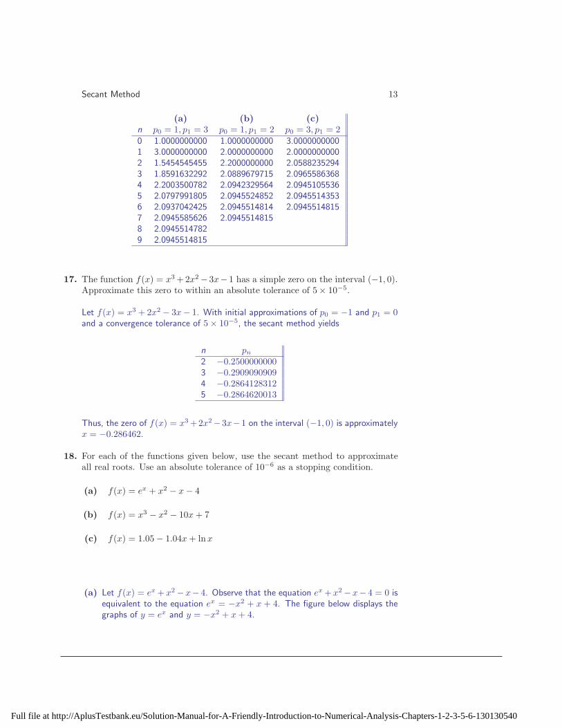
Secant Method 13
(a) (b) (c)n p0 = 1, p1 = 3 p0 = 1, p1 = 2 p0 = 3, p1 = 20 1.0000000000 1.0000000000 3.00000000001 3.0000000000 2.0000000000 2.00000000002 1.5454545455 2.2000000000 2.05882352943 1.8591632292 2.0889679715 2.09655863684 2.2003500782 2.0942329564 2.09451055365 2.0797991805 2.0945524852 2.09455143536 2.0937042425 2.0945514814 2.09455148157 2.0945585626 2.09455148158 2.09455147829 2.0945514815
17. The function f(x) = x3 +2x2 − 3x− 1 has a simple zero on the interval (−1, 0).Approximate this zero to within an absolute tolerance of 5× 10⁻⁵.
Let f(x) = x3 + 2x2 − 3x− 1. With initial approximations of p0 = −1 and p1 = 0and a convergence tolerance of 5 × 10⁻⁵, the secant method yields
n pn
2 −0.25000000003 −0.29090909094 −0.28641283125 −0.2864620013
Thus, the zero of f(x) = x3 +2x2−3x−1 on the interval (−1, 0) is approximatelyx = −0.286462.
18. For each of the functions given below, use the secant method to approximateall real roots. Use an absolute tolerance of 10−6 as a stopping condition.
(a) f(x) = ex + x2 − x − 4
(b) f(x) = x3 − x2 − 10x + 7
(c) f(x) = 1.05 − 1.04x + lnx
(a) Let f(x) = ex +x2 −x− 4. Observe that the equation ex +x2 −x− 4 = 0 isequivalent to the equation ex = −x2 + x + 4. The figure below displays thegraphs of y = ex and y = −x2 + x + 4.
Full file at http://AplusTestbank.eu/Solution-Manual-for-A-Friendly-Introduction-to-Numerical-Analysis-Chapters-1-2-3-5-6-130130540
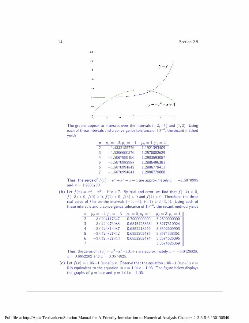
14 Section 2.5
The graphs appear to intersect over the intervals (−2,−1) and (1, 2). Usingeach of these intervals and a convergence tolerance of 10−6, the secant methodyields
n p0 = −2, p1 = −1 p0 = 1, p1 = 22 −1.4332155776 1.19213934093 −1.5206690376 1.25780826294 −1.5067999496 1.29035930875 −1.5070982988 1.28864963916 −1.5070994842 1.28867794117 −1.5070994841 1.2886779668
Thus, the zeros of f(x) = ex +x2 −x− 4 are approximately x = −1.5070995and x = 1.2886780.
(b) Let f(x) = x3 − x2 − 10x + 7. By trial and error, we find that f(−4) < 0,f(−3) > 0, f(0) > 0, f(1) < 0, f(3) < 0 and f(4) > 0. Therefore, the threereal zeros of f lie on the intervals (−4,−3), (0, 1) and (3, 4). Using each ofthese intervals and a convergence tolerance of 10−6, the secant method yields
n p0 = −4, p1 = −3 p0 = 0, p1 = 1 p0 = 3, p1 = 42 −3.0294117647 0.7000000000 3.25000000003 −3.0429276988 0.6845425868 3.32773109244 −3.0426813987 0.6852213246 3.35926099035 −3.0426827842 0.6852202475 3.35743383616 −3.0426827843 0.6852202474 3.35746250957 3.3574625369
Thus, the zeros of f(x) = x3−x2−10x+7 are approximately x = −3.0426828,x = 0.6852202 and x = 3.3574625.
(c) Let f(x) = 1.05−1.04x+ln x. Observe that the equation 1.05−1.04x+ln x =0 is equivalent to the equation lnx = 1.04x− 1.05. The figure below displaysthe graphs of y = lnx and y = 1.04x − 1.05.
Full file at http://AplusTestbank.eu/Solution-Manual-for-A-Friendly-Introduction-to-Numerical-Analysis-Chapters-1-2-3-5-6-130130540

Secant Method 15
The graphs appear to intersect over the intervals (0.80, 0.85) and (1.10, 1.15).Using each of these intervals and a convergence tolerance of 10−6, the secantmethod yields
n p0 = 0.80, p1 = 0.85 p0 = 1.10, p1 = 1.152 0.8298189963 1.10867871353 0.8268947961 1.10960533494 0.8271842009 1.10971262855 0.8271809126 1.10971230386 0.8271809085
Thus, the zeros of f(x) = 1.05−1.04x+ln x are approximately x = 0.8271809and x = 1.1097123.
19. Keller (“Probability of a Shutout in Racquetball,” SIAM Review, 26, 267-8,1984) showed that the probability that Player A will shut out Player B in agame of racquetball is given by
P =1 + w
2
(
w
1 − w + w2
)21
,
where w denotes the probability that Player A will win any specific rally, inde-pendent of the server. Determine the minimal value of w that will guaranteethat Player A will shut out Player B in at least one-quarter of the games theyplay. Repeat your calculations for at least half the games being shutouts andat least three-quarters of the games being shutouts.
Let
f(w) =1 + w
2
(
w
1 − w + w2
)21
− P.
For various values of P, the following table displays the results obtained from thesecant method. In each case, w0 = 0.5, w1 = 1 and ǫ = 5 × 10⁻⁷.
Full file at http://AplusTestbank.eu/Solution-Manual-for-A-Friendly-Introduction-to-Numerical-Analysis-Chapters-1-2-3-5-6-130130540

16 Section 2.5
n P = 0.25 P = 0.50 P = 0.752 0.6249436049 0.7499624033 0.87498120163 0.7154534705 0.8506640530 0.91161350754 0.8988222452 0.8406140860 0.89985195405 0.7599522840 0.8422953603 0.89917640386 0.7749547792 0.8423048039 0.89919897877 0.7799794811 0.8423047910 0.89919894258 0.77957844019 0.779585535110 0.7795855457
Thus, for Player A to shut out Player B in at least one-quarter of the games theyplay, Player A must win any specific rally with a probability of 77.96%. To shut outPalyer B at least one-half of the time, the probability of winning any specific rallymust rise to 84.23%. Finally, to shut out Player B at least three-quarters of thetime, the probability of winning any specific rally must rise to 89.92%.
20. A couple wishes to open a money market account in which they will save thedown payment for purchasing a house. The couple has $13,000 from the sale ofsome stock with which to open the account and plans to deposit an additional$200 each month thereafter. By the end of three years, the couple hopes tohave saved $20,000. If the money market account pays an annual interest ofr%, compounded monthly, then at the end of three years, the balance of theaccount will be
13000(
1 +r
12
)36
+ 200
(
1 + r12
)36 − 1r12
.
What is the lowest interest rate which will achieve the couple’s goal of saving$20,000? What is the lowest interest rate if the couple can raise their monthlydeposit to $250?
To reach a goal of $20,000, the couple does not need to earn any interest. Let’swork the problem with a goal of $25,000. Let
f(r) = 13000(
1 +r
12
)36
+ 200
(
1 + r12
)36 − 1
r/12− 25000.
Because f(0.05) ≈ −2150.19 and f(0.1) ≈ 882.73, we take r0 = 0.05 and r1 = 0.1.With a convergence tolerance of 5 × 10⁻⁶, the secant method yields
n rn
2 0.085447563 0.086118314 0.086131055 0.08613104
Thus, the couple needs to find an account which yields at least 8.61%, compounded
Full file at http://AplusTestbank.eu/Solution-Manual-for-A-Friendly-Introduction-to-Numerical-Analysis-Chapters-1-2-3-5-6-130130540
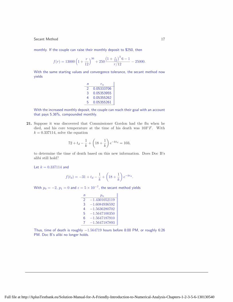
Secant Method 17
monthly. If the couple can raise their monthly deposit to $250, then
f(r) = 13000(
1 +r
12
)36
+ 250
(
1 + r12
)36 − 1
r/12− 25000.
With the same starting values and convergence tolerance, the secant method nowyields
n rn
2 0.053337063 0.053539554 0.053552625 0.05355261
With the increased monthly deposit, the couple can reach their goal with an accountthat pays 5.36%, compounded monthly.
21. Suppose it was discovered that Commissioner Gordon had the flu when hedied, and his core temperature at the time of his death was 103◦F . Withk = 0.337114, solve the equation
72 + td − 1
k+
(
18 +1
k
)
e−ktd = 103,
to determine the time of death based on this new information. Does Doc B’salibi still hold?
Let k = 0.337114 and
f(td) = −31 + td − 1
k+
(
18 +1
k
)
e−ktd .
With p0 = −2, p1 = 0 and ǫ = 5 × 10⁻⁷, the secant method yields
n pn
2 −1.43010521193 −1.60849365924 −1.56362807025 −1.56471003506 −1.56471879107 −1.5647187893
Thus, time of death is roughly −1.564719 hours before 8:00 PM, or roughly 6:26PM. Doc B’s alibi no longer holds.
Full file at http://AplusTestbank.eu/Solution-Manual-for-A-Friendly-Introduction-to-Numerical-Analysis-Chapters-1-2-3-5-6-130130540

Accelerating Convergence 1
2.6 Accelerating Convergence
1. Show that the equation for Aitken’s ∆2-method can be rewritten as
p̂n =pnpn−2 − p2
n−1
pn − 2pn−1 + pn−2
.
Explain why this formula is inferior to the one used in the text.
Combining the terms on the right-hand side of the formula yields
p̂n = pn − (pn − pn−1)2
pn + pn−2 − 2pn−1
=p2
n+ pnpn−2 − 2pnpn−1 − p2
n+ 2pnpn−1 + p2
n−1
pn + pn−2 − 2pn−1
=pnpn−2 − p2
n−1
pn + pn−2 − 2pn−1
.
Note that both formulas for calculating p̂n have the potential for cancellation error.In the formula
p̂n = pn − (pn − pn−1)2
pn + pn−2 − 2pn−1
,
cancellation error will primarily influence the second term, which is essentially justa correction to pn. This can limit the overall effect of roundoff error on p̂n. In theformula
p̂n =pnpn−2 − p2
n−1
pn + pn−2 − 2pn−1
,
however, cancellation error influences the entire calculation. Thus, the latter formulais inferior to the former because it is more susceptible to roundoff error.
2. Should Aitken’s ∆2-method be applied to a sequence generated by the bisectionmethod? Explain.
Aitken’s ∆2-method is designed to accelerate the convergence of linearly convergentsequences. Recall that though the general trend over several terms in the bisectionsequence is linear, the sequence does not technically converge linearly. Consequently,Aitken’s ∆2-method should not be applied a sequence generated by the bisectionmethod.
Full file at http://AplusTestbank.eu/Solution-Manual-for-A-Friendly-Introduction-to-Numerical-Analysis-Chapters-1-2-3-5-6-130130540

2 Section 2.6
3. The sequence listed below was obtained from the method of false position ap-plied to the function f(x) = tan(πx) − x − 6 over the interval (0.40, 0.48).
1 0.4208674112 0.4332027503 0.4404957394 0.4448079255 0.4473577486 0.4488655167 0.449757107
(a) Apply Aitken’s ∆2-method to the given sequence.
(b) To nine digits, the zero of f on (0.40, 0.48) is x = 0.451047259. Use thisto show that both the original sequence and the output from Aitken’s ∆2-method are linearly convergent and estimate the corresponding asymptoticerror constants. By how much has Aitken’s ∆2-method reduced the asymp-totic error constant?
(a) Using the first three terms in the False Position sequence, we calculate
p̂3 = p3 −(p3 − p2)
2
p3 + p1 − 2p2
= 0.440495739 − (0.440495739 − 0.433202750)2
0.440495739 + 0.420867411 − 2(0.433202750)
= 0.451043933.
Next, using p2, p3 and p4, we calculate
p̂4 = p4 −(p4 − p3)
2
p4 + p2 − 2p3
= 0.444807925 − (0.444807925 − 0.440495739)2
0.444807925 + 0.433202750 − 2(0.440495739)
= 0.451046159.
Continuing in this manner, we find
p̂5 = 0.451046884, p̂6 = 0.451047132, and p̂7 = 0.451047214.
(b) The values in columns 3 and 5 in the table below confirm that both the originalFalse Position sequence and the accelerated seqeunce converge linearly. Theasymptotic error constant for the False Position sequence is 0.5913, whilethe asymptotic error constant for the accelerated sequence is roughly 0.34.
Full file at http://AplusTestbank.eu/Solution-Manual-for-A-Friendly-Introduction-to-Numerical-Analysis-Chapters-1-2-3-5-6-130130540
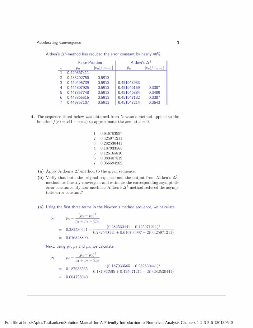
Accelerating Convergence 3
Aitken’s ∆2-method has reduced the error constant by nearly 40%.
False Position Aitken’s ∆2
n pn |en|/|en−1| p̂n |en|/|en−1|1 0.4208674112 0.433202750 0.59133 0.440495739 0.5913 0.4510439334 0.444807925 0.5913 0.451046159 0.33075 0.447357748 0.5913 0.451046884 0.34096 0.448865516 0.5913 0.451047132 0.33877 0.449757107 0.5913 0.451047214 0.3543
4. The sequence listed below was obtained from Newton’s method applied to thefunction f(x) = x(1 − cos x) to approximate the zero at x = 0.
1 0.6467039972 0.4259712113 0.2825304414 0.1879335655 0.1251658106 0.0834075197 0.055594262
(a) Apply Aitken’s ∆2-method to the given sequence.
(b) Verify that both the original sequence and the output from Aitken’s ∆2-method are linearly convergent and estimate the corresponding asymptoticerror constants. By how much has Aitken’s ∆2-method reduced the asymp-totic error constant?
(a) Using the first three terms in the Newton’s method sequence, we calculate
p̂3 = p3 −(p3 − p2)
2
p3 + p1 − 2p2
= 0.282530441 − (0.282530441 − 0.425971211)2
0.282530441 + 0.646703997 − 2(0.425971211)
= 0.016328890.
Next, using p2, p3 and p4, we calculate
p̂4 = p4 −(p4 − p3)
2
p4 + p2 − 2p3
= 0.187933565 − (0.187933565 − 0.282530441)2
0.187933565 + 0.425971211 − 2(0.282530441)
= 0.004726040.
Full file at http://AplusTestbank.eu/Solution-Manual-for-A-Friendly-Introduction-to-Numerical-Analysis-Chapters-1-2-3-5-6-130130540
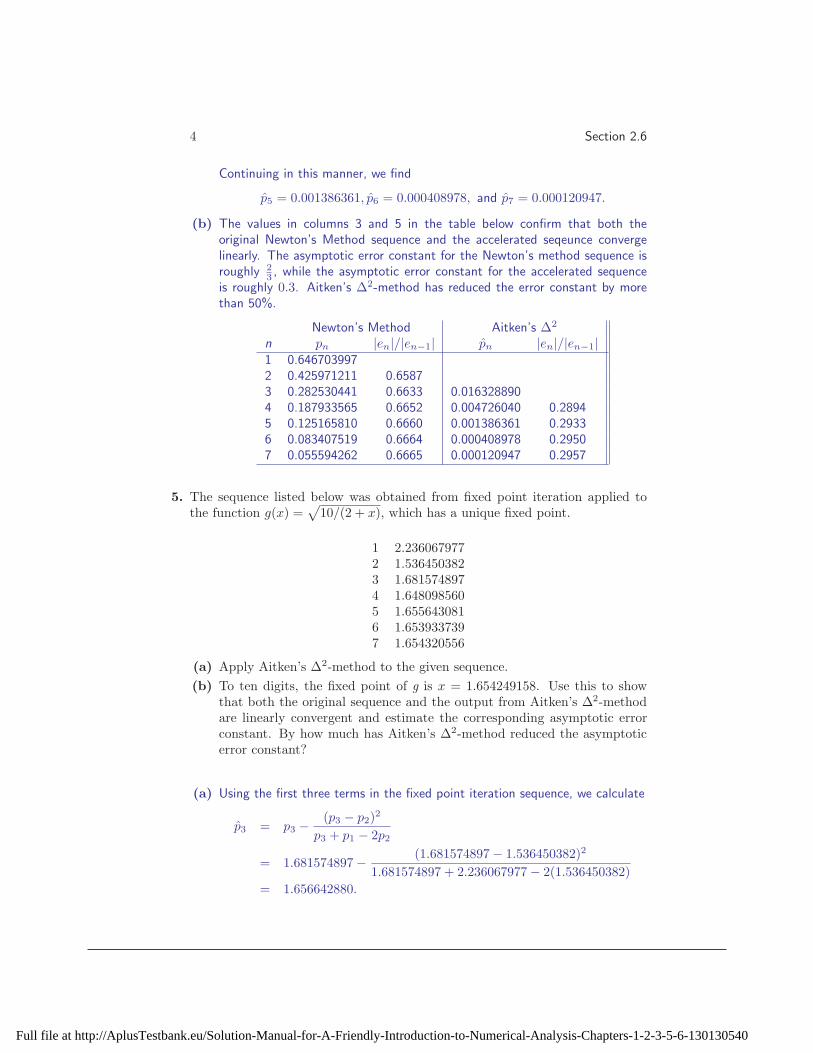
4 Section 2.6
Continuing in this manner, we find
p̂5 = 0.001386361, p̂6 = 0.000408978, and p̂7 = 0.000120947.
(b) The values in columns 3 and 5 in the table below confirm that both theoriginal Newton’s Method sequence and the accelerated seqeunce convergelinearly. The asymptotic error constant for the Newton’s method sequence isroughly 2
3, while the asymptotic error constant for the accelerated sequence
is roughly 0.3. Aitken’s ∆2-method has reduced the error constant by morethan 50%.
Newton’s Method Aitken’s ∆2
n pn |en|/|en−1| p̂n |en|/|en−1|1 0.6467039972 0.425971211 0.65873 0.282530441 0.6633 0.0163288904 0.187933565 0.6652 0.004726040 0.28945 0.125165810 0.6660 0.001386361 0.29336 0.083407519 0.6664 0.000408978 0.29507 0.055594262 0.6665 0.000120947 0.2957
5. The sequence listed below was obtained from fixed point iteration applied tothe function g(x) =
√
10/(2 + x), which has a unique fixed point.
1 2.2360679772 1.5364503823 1.6815748974 1.6480985605 1.6556430816 1.6539337397 1.654320556
(a) Apply Aitken’s ∆2-method to the given sequence.
(b) To ten digits, the fixed point of g is x = 1.654249158. Use this to showthat both the original sequence and the output from Aitken’s ∆2-methodare linearly convergent and estimate the corresponding asymptotic errorconstant. By how much has Aitken’s ∆2-method reduced the asymptoticerror constant?
(a) Using the first three terms in the fixed point iteration sequence, we calculate
p̂3 = p3 −(p3 − p2)
2
p3 + p1 − 2p2
= 1.681574897 − (1.681574897 − 1.536450382)2
1.681574897 + 2.236067977 − 2(1.536450382)
= 1.656642880.
Full file at http://AplusTestbank.eu/Solution-Manual-for-A-Friendly-Introduction-to-Numerical-Analysis-Chapters-1-2-3-5-6-130130540
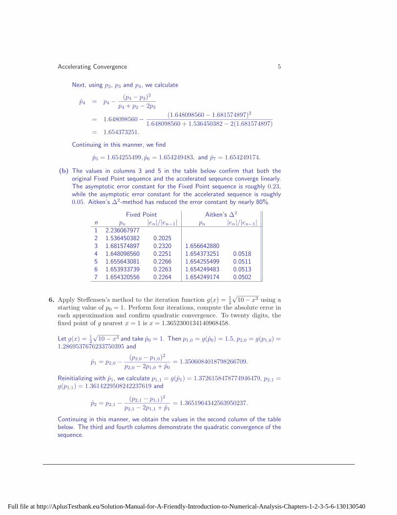
Accelerating Convergence 5
Next, using p2, p3 and p4, we calculate
p̂4 = p4 −(p4 − p3)
2
p4 + p2 − 2p3
= 1.648098560 − (1.648098560 − 1.681574897)2
1.648098560 + 1.536450382 − 2(1.681574897)
= 1.654373251.
Continuing in this manner, we find
p̂5 = 1.654255499, p̂6 = 1.654249483, and p̂7 = 1.654249174.
(b) The values in columns 3 and 5 in the table below confirm that both theoriginal Fixed Point sequence and the accelerated seqeunce converge linearly.The asymptotic error constant for the Fixed Point sequence is roughly 0.23,while the asymptotic error constant for the accelerated sequence is roughly0.05. Aitken’s ∆2-method has reduced the error constant by nearly 80%.
Fixed Point Aitken’s ∆2
n pn |en|/|en−1| pn |en|/|en−1|1 2.2360679772 1.536450382 0.20253 1.681574897 0.2320 1.6566428804 1.648098560 0.2251 1.654373251 0.05185 1.655643081 0.2266 1.654255499 0.05116 1.653933739 0.2263 1.654249483 0.05137 1.654320556 0.2264 1.654249174 0.0502
6. Apply Steffensen’s method to the iteration function g(x) = 1
2
√10 − x3 using a
starting value of p0 = 1. Perform four iterations, compute the absolute error ineach approximation and confirm quadratic convergence. To twenty digits, thefixed point of g nearest x = 1 is x = 1.3652300134140968458.
Let g(x) = 1
2
√10 − x3 and take p̂0 = 1. Then p1,0 = g(p̂0) = 1.5, p2,0 = g(p1,0) =
1.2869537676233750395 and
p̂1 = p2,0 −(p2,0 − p1,0)
2
p2,0 − 2p1,0 + p̂0
= 1.3506084018798266709.
Reinitializing with p̂1, we calculate p1,1 = g(p̂1) = 1.3726158478774946479, p2,1 =g(p1,1) = 1.3614229508242237619 and
p̂2 = p2,1 −(p2,1 − p1,1)
2
p2,1 − 2p1,1 + p̂1
= 1.3651964342563950237.
Continuing in this manner, we obtain the values in the second column of the tablebelow. The third and fourth columns demonstrate the quadratic convergence of thesequence.
Full file at http://AplusTestbank.eu/Solution-Manual-for-A-Friendly-Introduction-to-Numerical-Analysis-Chapters-1-2-3-5-6-130130540
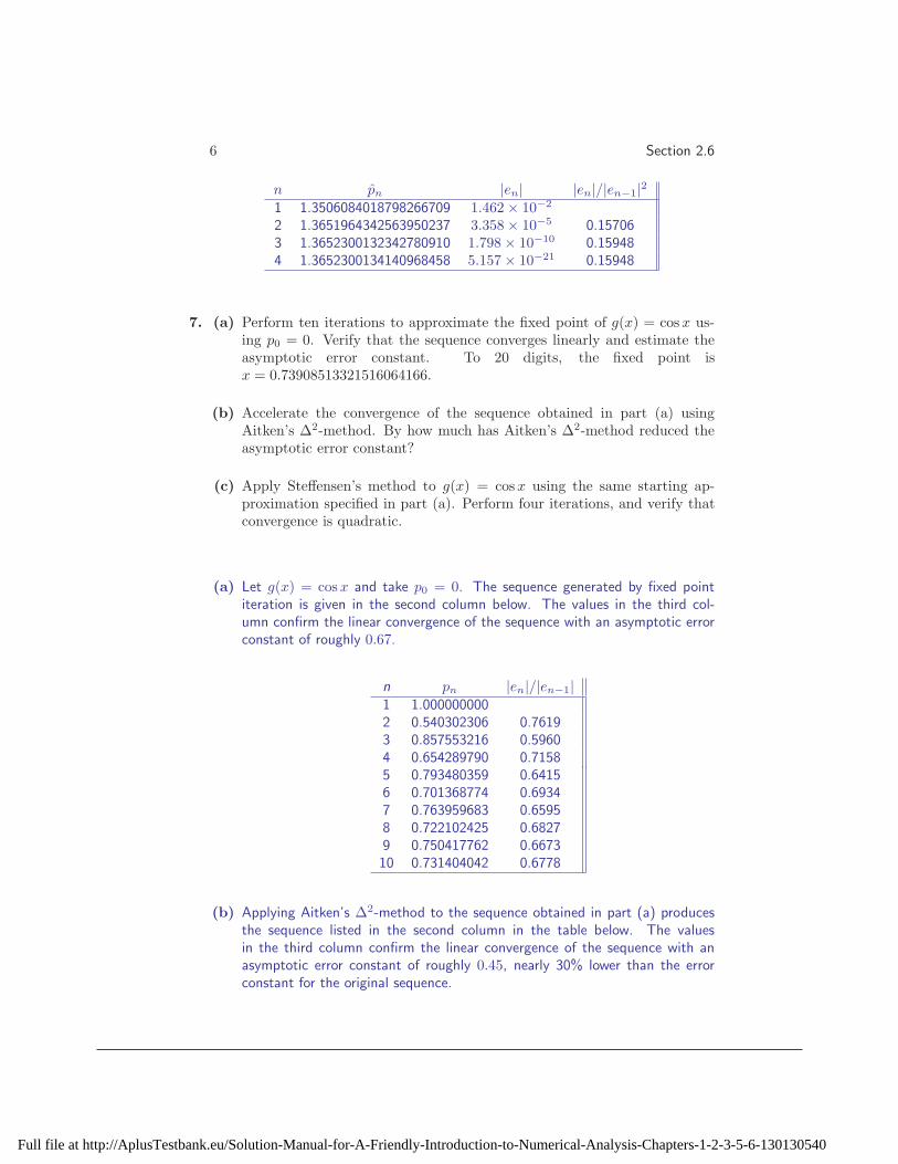
6 Section 2.6
n p̂n |en| |en|/|en−1|21 1.3506084018798266709 1.462 × 10⁻²
2 1.3651964342563950237 3.358 × 10⁻⁵ 0.157063 1.3652300132342780910 1.798 × 10⁻¹⁰ 0.159484 1.3652300134140968458 5.157 × 10⁻²¹ 0.15948
7. (a) Perform ten iterations to approximate the fixed point of g(x) = cos x us-ing p0 = 0. Verify that the sequence converges linearly and estimate theasymptotic error constant. To 20 digits, the fixed point isx = 0.73908513321516064166.
(b) Accelerate the convergence of the sequence obtained in part (a) usingAitken’s ∆2-method. By how much has Aitken’s ∆2-method reduced theasymptotic error constant?
(c) Apply Steffensen’s method to g(x) = cos x using the same starting ap-proximation specified in part (a). Perform four iterations, and verify thatconvergence is quadratic.
(a) Let g(x) = cos x and take p0 = 0. The sequence generated by fixed pointiteration is given in the second column below. The values in the third col-umn confirm the linear convergence of the sequence with an asymptotic errorconstant of roughly 0.67.
n pn |en|/|en−1|1 1.0000000002 0.540302306 0.76193 0.857553216 0.59604 0.654289790 0.71585 0.793480359 0.64156 0.701368774 0.69347 0.763959683 0.65958 0.722102425 0.68279 0.750417762 0.667310 0.731404042 0.6778
(b) Applying Aitken’s ∆2-method to the sequence obtained in part (a) producesthe sequence listed in the second column in the table below. The valuesin the third column confirm the linear convergence of the sequence with anasymptotic error constant of roughly 0.45, nearly 30% lower than the errorconstant for the original sequence.
Full file at http://AplusTestbank.eu/Solution-Manual-for-A-Friendly-Introduction-to-Numerical-Analysis-Chapters-1-2-3-5-6-130130540

Accelerating Convergence 7
n p̂n |en|/|en−1|3 0.7280103614 0.733665165 0.48945 0.736906294 0.40206 0.738050421 0.47497 0.738636097 0.43408 0.738876583 0.46449 0.738992243 0.445410 0.739042511 0.4588
(c) Let g(x) = cos x and take p̂0 = 0. Steffensen’s method produces the sequencegiven in the second column of the table below. The values in the third columnconfirm quadratic convergence of the sequence.
n p̂n |en|/|en−1|21 0.6850733573260452 0.738660156167713 0.14573 0.739085106356719 0.14874 0.739085133215160 0.1539
8. (a) Perform ten iterations to approximate the fixed point of g(x) = ln(4 +x − x2) using p0 = 2. Verify that the sequence converges linearly andestimate the asymptotic error constant. To 20 digits, the fixed point isx = 1.2886779668238684115.
(b) Accelerate the convergence of the sequence obtained in part (a) usingAitken’s ∆2-method. By how much has Aitken’s ∆2-method reduced theasymptotic error constant?
(c) Apply Steffensen’s method to g(x) = ln(4+x−x2) using the same startingapproximation specified in part (a). Perform four iterations, and verifythat convergence is quadratic.
(a) Let g(x) = ln(4 + x− x2) and take p0 = 2. The sequence generated by fixedpoint iteration is given in the second column below. The values in the thirdcolumn confirm the linear convergence of the sequence with an asymptoticerror constant of roughly 0.44.
n pn |en|/|en−1|1 0.69314718062 1.438102388 0.25093 1.214902035 0.49374 1.318795484 0.40825 1.275243786 0.44616 1.294452355 0.42987 1.286155040 0.43698 1.289772517 0.43389 1.288201641 0.435210 1.288884977 0.4346
Full file at http://AplusTestbank.eu/Solution-Manual-for-A-Friendly-Introduction-to-Numerical-Analysis-Chapters-1-2-3-5-6-130130540

8 Section 2.6
(b) Applying Aitken’s ∆2-method to the sequence obtained in part (a) producesthe sequence listed in the second column in the table below. The valuesin the third column confirm the linear convergence of the sequence with anasymptotic error constant of roughly 0.19, more than 50% lower than the errorconstant for the original sequence.
n p̂n |en|/|en−1|3 1.2663590524 1.285796238 0.12915 1.288107895 0.19786 1.288573331 0.18357 1.288657975 0.19118 1.288674207 0.18819 1.288677255 0.189410 1.288677832 0.1896
(c) Let g(x) = ln(4+x−x2) and take p̂0 = 2. Steffensen’s method produces thesequence given in the second column of the table below. The values in thethird column confirm quadratic convergence of the sequence.
n p̂n |en|/|en−1|21 1.167629588320392 1.28720918451180 0.10023 1.28867772517834 0.11204 1.28867796682386 0.1122
9. (a) Perform ten iterations to approximate the fixed point of g(x) = (1.05 +lnx)/1.04 using p0 = 1. Verify that the sequence converges linearly andestimate the asymptotic error constant. To 20 digits, the fixed point isx = 1.1097123038867133005.
(b) Accelerate the convergence of the sequence obtained in part (a) usingAitken’s ∆2-method. By how much has Aitken’s ∆2-method reduced theasymptotic error constant?
(c) Apply Steffensen’s method to g(x) = (1.05 + lnx)/1.04 using the samestarting approximation specified in part (a). Perform five iterations, andverify that convergence is quadratic.
(a) Let g(x) = (1.05 + lnx)/1.04 and take p0 = 1. The sequence generatedby fixed point iteration is given in the second column below. The valuesin the third column confirm the linear convergence of the sequence with anasymptotic error constant of roughly 0.88.
Full file at http://AplusTestbank.eu/Solution-Manual-for-A-Friendly-Introduction-to-Numerical-Analysis-Chapters-1-2-3-5-6-130130540
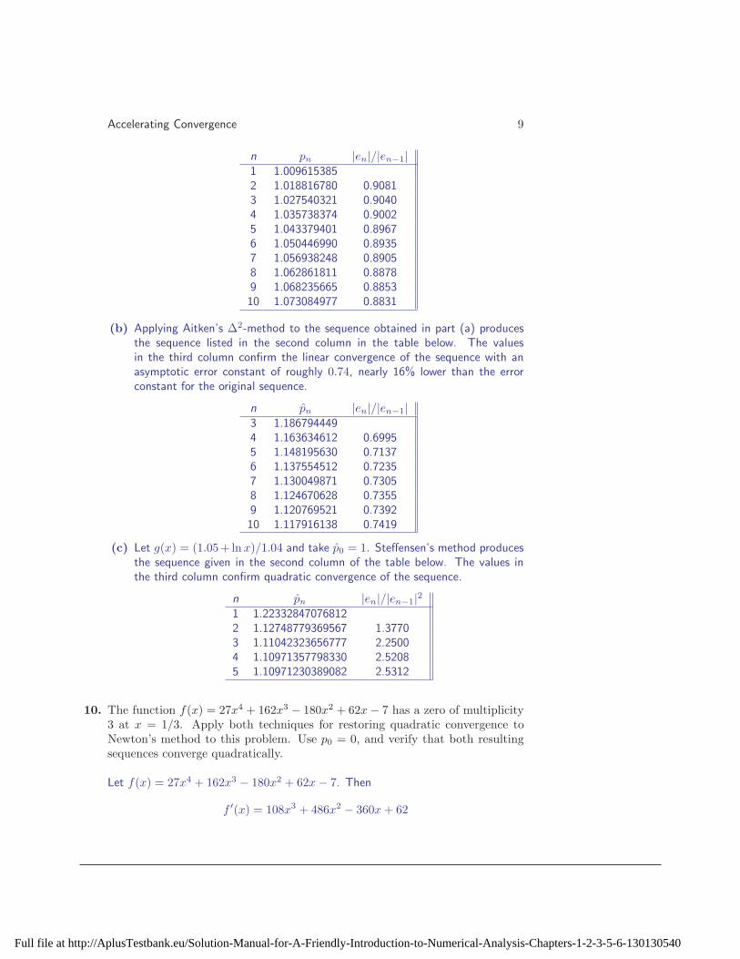
Accelerating Convergence 9
n pn |en|/|en−1|1 1.0096153852 1.018816780 0.90813 1.027540321 0.90404 1.035738374 0.90025 1.043379401 0.89676 1.050446990 0.89357 1.056938248 0.89058 1.062861811 0.88789 1.068235665 0.885310 1.073084977 0.8831
(b) Applying Aitken’s ∆2-method to the sequence obtained in part (a) producesthe sequence listed in the second column in the table below. The valuesin the third column confirm the linear convergence of the sequence with anasymptotic error constant of roughly 0.74, nearly 16% lower than the errorconstant for the original sequence.
n p̂n |en|/|en−1|3 1.1867944494 1.163634612 0.69955 1.148195630 0.71376 1.137554512 0.72357 1.130049871 0.73058 1.124670628 0.73559 1.120769521 0.739210 1.117916138 0.7419
(c) Let g(x) = (1.05+ lnx)/1.04 and take p̂0 = 1. Steffensen’s method producesthe sequence given in the second column of the table below. The values inthe third column confirm quadratic convergence of the sequence.
n p̂n |en|/|en−1|21 1.223328470768122 1.12748779369567 1.37703 1.11042323656777 2.25004 1.10971357798330 2.52085 1.10971230389082 2.5312
10. The function f(x) = 27x4 + 162x3 − 180x2 + 62x − 7 has a zero of multiplicity3 at x = 1/3. Apply both techniques for restoring quadratic convergence toNewton’s method to this problem. Use p0 = 0, and verify that both resultingsequences converge quadratically.
Let f(x) = 27x4 + 162x3 − 180x2 + 62x − 7. Then
f ′(x) = 108x3 + 486x2 − 360x + 62
Full file at http://AplusTestbank.eu/Solution-Manual-for-A-Friendly-Introduction-to-Numerical-Analysis-Chapters-1-2-3-5-6-130130540
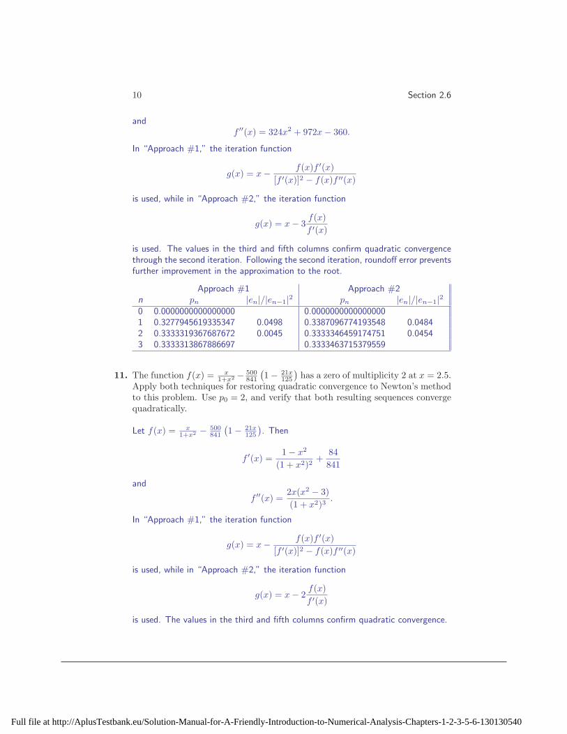
10 Section 2.6
andf ′′(x) = 324x2 + 972x − 360.
In “Approach #1,” the iteration function
g(x) = x − f(x)f ′(x)
[f ′(x)]2 − f(x)f ′′(x)
is used, while in “Approach #2,” the iteration function
g(x) = x − 3f(x)
f ′(x)
is used. The values in the third and fifth columns confirm quadratic convergencethrough the second iteration. Following the second iteration, roundoff error preventsfurther improvement in the approximation to the root.
Approach #1 Approach #2n pn |en|/|en−1|2 pn |en|/|en−1|20 0.0000000000000000 0.00000000000000001 0.3277945619335347 0.0498 0.3387096774193548 0.04842 0.3333319367687672 0.0045 0.3333346459174751 0.04543 0.3333313867886697 0.3333463715379559
11. The function f(x) = x
1+x2 − 500
841
(
1 − 21x
125
)
has a zero of multiplicity 2 at x = 2.5.Apply both techniques for restoring quadratic convergence to Newton’s methodto this problem. Use p0 = 2, and verify that both resulting sequences convergequadratically.
Let f(x) = x
1+x2 − 500
841
(
1 − 21x
125
)
. Then
f ′(x) =1 − x2
(1 + x2)2+
84
841
and
f ′′(x) =2x(x2 − 3)
(1 + x2)3.
In “Approach #1,” the iteration function
g(x) = x − f(x)f ′(x)
[f ′(x)]2 − f(x)f ′′(x)
is used, while in “Approach #2,” the iteration function
g(x) = x − 2f(x)
f ′(x)
is used. The values in the third and fifth columns confirm quadratic convergence.
Full file at http://AplusTestbank.eu/Solution-Manual-for-A-Friendly-Introduction-to-Numerical-Analysis-Chapters-1-2-3-5-6-130130540

Accelerating Convergence 11
Approach #1 Approach #2n pn |en|/|en−1|2 pn |en|/|en−1|20 2.000000000000000 2.0000000000000001 2.443476520429667 0.2261 2.520094562647761 0.08042 2.500026470879555 0.0083 2.499990347448545 0.02393 2.500000000017783 0.0254 2.499999999989277 0.1151
12. The function f(x) = x(1 − cos x) has a zero of multiplicity 3 at x = 0. Applyboth techniques for restoring quadratic convergence to Newton’s method to thisproblem, using p0 = 1. You should observe that the resulting sequences appearto converge faster than quadratically. What apparent order of convergence doyou observe? Why is convergence faster than quadratic for this problem?
Let f(x) = x(1 − cos x). Then f ′(x) = x sinx + 1 − cos x and f ′′(x) = x cos x +2 sin x. In “Approach #1,” the iteration function
g(x) = x − f(x)f ′(x)
[f ′(x)]2 − f(x)f ′′(x)
is used, while in “Approach #2,” the iteration function
g(x) = x − 2f(x)
f ′(x)
is used. To explore the order of convergence fully, the values below were obtainedusing Maple with the Digits parameter set to 100.
Approach #1 Approach #2n pn pn
1 1.0860 × 10⁻¹ −5.9888 × 10⁻²
2 1.4229 × 10⁻⁴ 1.1936 × 10⁻⁵
3 3.2011 × 10⁻¹³ −9.4473 × 10⁻¹⁷
4 3.6447 × 10−39 4.6843 × 10−50
Recall the root of this function is x = 0. The values above suggest that both se-quences are converging of order three, which is better than expected from Newton’smethod. This better than expected performance occurs because in the “modified”function, the second derivative at x = 0 is zero.
13. Suppose Newton’s method is applied to a function with a zero of multiplicitym > 1. Show that the multiplicity of the zero can be estimated as the integernearest to
m ≈ 1
1 − pn−pn−1
pn−1−pn−2
.
Verify that this formula produces an accurate estimate when applied to thesequence listed in Exercise 4 and when applied to the sequence generated whenNewton’s method was applied to the function f(x) = 1 + lnx − x in the text.
Full file at http://AplusTestbank.eu/Solution-Manual-for-A-Friendly-Introduction-to-Numerical-Analysis-Chapters-1-2-3-5-6-130130540
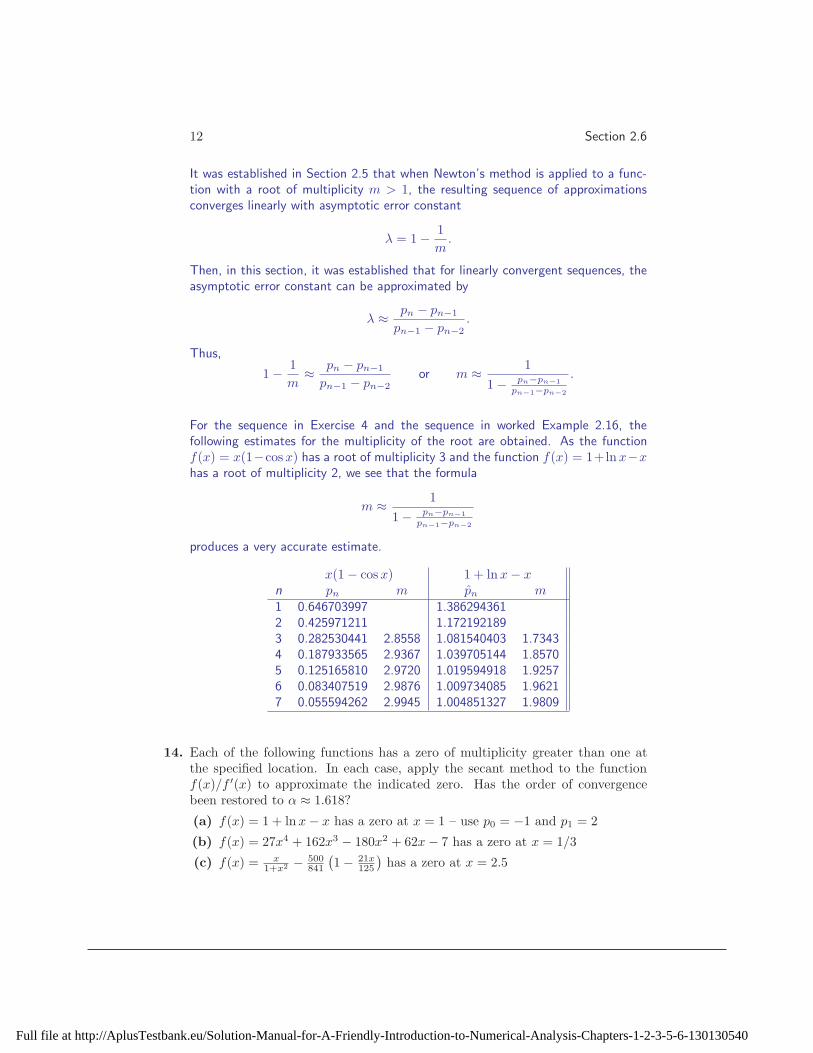
12 Section 2.6
It was established in Section 2.5 that when Newton’s method is applied to a func-tion with a root of multiplicity m > 1, the resulting sequence of approximationsconverges linearly with asymptotic error constant
λ = 1 − 1
m.
Then, in this section, it was established that for linearly convergent sequences, theasymptotic error constant can be approximated by
λ ≈ pn − pn−1
pn−1 − pn−2
.
Thus,
1 − 1
m≈ pn − pn−1
pn−1 − pn−2
or m ≈ 1
1 − pn−pn−1
pn−1−pn−2
.
For the sequence in Exercise 4 and the sequence in worked Example 2.16, thefollowing estimates for the multiplicity of the root are obtained. As the functionf(x) = x(1−cos x) has a root of multiplicity 3 and the function f(x) = 1+lnx−xhas a root of multiplicity 2, we see that the formula
m ≈ 1
1 − pn−pn−1
pn−1−pn−2
produces a very accurate estimate.
x(1 − cos x) 1 + lnx − xn pn m p̂n m1 0.646703997 1.3862943612 0.425971211 1.1721921893 0.282530441 2.8558 1.081540403 1.73434 0.187933565 2.9367 1.039705144 1.85705 0.125165810 2.9720 1.019594918 1.92576 0.083407519 2.9876 1.009734085 1.96217 0.055594262 2.9945 1.004851327 1.9809
14. Each of the following functions has a zero of multiplicity greater than one atthe specified location. In each case, apply the secant method to the functionf(x)/f ′(x) to approximate the indicated zero. Has the order of convergencebeen restored to α ≈ 1.618?
(a) f(x) = 1 + lnx − x has a zero at x = 1 – use p0 = −1 and p1 = 2
(b) f(x) = 27x4 + 162x3 − 180x2 + 62x − 7 has a zero at x = 1/3
(c) f(x) = x
1+x2 − 500
841
(
1 − 21x
125
)
has a zero at x = 2.5
Full file at http://AplusTestbank.eu/Solution-Manual-for-A-Friendly-Introduction-to-Numerical-Analysis-Chapters-1-2-3-5-6-130130540
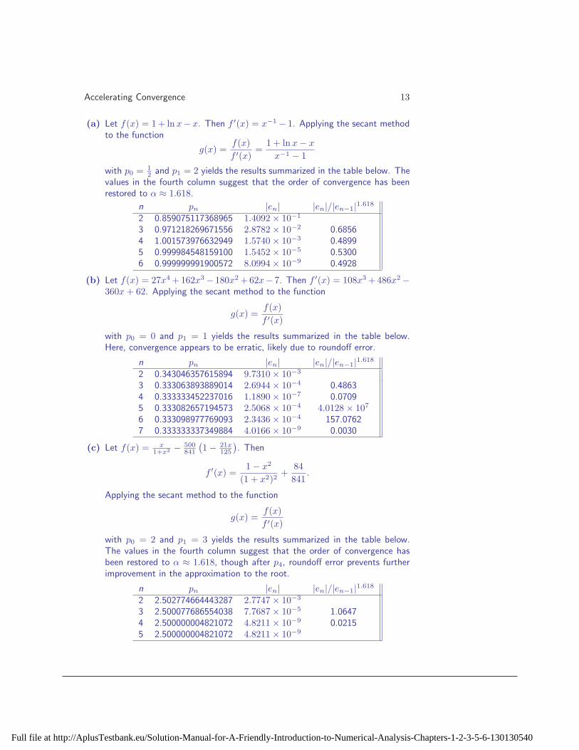
Accelerating Convergence 13
(a) Let f(x) = 1 + lnx− x. Then f ′(x) = x−1 − 1. Applying the secant methodto the function
g(x) =f(x)
f ′(x)=
1 + lnx − x
x−1 − 1
with p0 = 1
2and p1 = 2 yields the results summarized in the table below. The
values in the fourth column suggest that the order of convergence has beenrestored to α ≈ 1.618.
n pn |en| |en|/|en−1|1.618
2 0.859075117368965 1.4092 × 10⁻¹
3 0.971218269671556 2.8782 × 10⁻² 0.68564 1.001573976632949 1.5740 × 10⁻³ 0.48995 0.999984548159100 1.5452 × 10⁻⁵ 0.53006 0.999999991900572 8.0994 × 10⁻⁹ 0.4928
(b) Let f(x) = 27x4 +162x3 − 180x2 +62x− 7. Then f ′(x) = 108x3 +486x2 −360x + 62. Applying the secant method to the function
g(x) =f(x)
f ′(x)
with p0 = 0 and p1 = 1 yields the results summarized in the table below.Here, convergence appears to be erratic, likely due to roundoff error.
n pn |en| |en|/|en−1|1.618
2 0.343046357615894 9.7310 × 10⁻³
3 0.333063893889014 2.6944 × 10⁻⁴ 0.48634 0.333333452237016 1.1890 × 10⁻⁷ 0.07095 0.333082657194573 2.5068 × 10⁻⁴ 4.0128 × 10⁷
6 0.333098977769093 2.3436 × 10⁻⁴ 157.07627 0.333333337349884 4.0166 × 10⁻⁹ 0.0030
(c) Let f(x) = x
1+x2 − 500
841
(
1 − 21x
125
)
. Then
f ′(x) =1 − x2
(1 + x2)2+
84
841.
Applying the secant method to the function
g(x) =f(x)
f ′(x)
with p0 = 2 and p1 = 3 yields the results summarized in the table below.The values in the fourth column suggest that the order of convergence hasbeen restored to α ≈ 1.618, though after p4, roundoff error prevents furtherimprovement in the approximation to the root.
n pn |en| |en|/|en−1|1.618
2 2.502774664443287 2.7747 × 10⁻³
3 2.500077686554038 7.7687 × 10⁻⁵ 1.06474 2.500000004821072 4.8211 × 10⁻⁹ 0.02155 2.500000004821072 4.8211 × 10⁻⁹
Full file at http://AplusTestbank.eu/Solution-Manual-for-A-Friendly-Introduction-to-Numerical-Analysis-Chapters-1-2-3-5-6-130130540

14 Section 2.6
15. Repeat Exercise 14, but this time replace the standard secant method formulafor pn+1 by the formula
pn+1 = pn − mf(pn)pn − pn−1
f(pn) − f(pn−1),
where m is the multiplicity of the zero being approximated. The functions in(a) and (c) have m = 2, and the function in (b) has m = 3.
Let f(x) = 1 + lnx − x. As x = 1 is a root of f(x) of multiplicity 2, we attemptthe iteration function
pn+1 = pn − 2f(pn)pn − pn−1
f(pn) − f(pn−1).
With p0 = 0.5 and p1 = 2, the following sequence is produced
p2 = −6.095978968
p3 = 9.612752412 + 0.1648235604i
p4 = −2.972344498 + 2.437342132i
p5 = 8.476800312 + 0.241149696i
p6 = −3.038729588 + 2.233167032i
etc. Clearly this sequence is not converging. Even with p0 = 0.9 and p1 = 1.1,a divergent sequence is produced. Divergent sequences result for the other twofunctions from Exercise 14 as well.
16. The method of false position and fixed point iteration generate linearly conver-gent sequences for which
limn→∞
pn − p
pn−1 − p(1)
exists. Note that this limit does not involve absolute values. Let λ denotethe value of this limit. This exercise will lead us through the proof that thesequence produced by Aitken’s ∆2-method converges more rapidly than linearlyconvergent sequences for which (6) exists.
(a) Let
ǫn =pn − p
pn−1 − p− λ.
Show that ǫn → 0 as n → ∞.
(b) Show that
∆pn = (pn − p)
(
1 − 1
ǫn + λ
)
.
(c) Show that
∆2pn = (pn − p)
[
1 − 1
ǫn + λ− 1
ǫn + λ
(
1 − 1
ǫn−1 + λ
)]
=pn − p
(ǫn + λ)(ǫn−1 + λ)
[
(λ − 1)2 + ǫ′n
]
,
Full file at http://AplusTestbank.eu/Solution-Manual-for-A-Friendly-Introduction-to-Numerical-Analysis-Chapters-1-2-3-5-6-130130540

Accelerating Convergence 15
where ǫ′n
= ǫnǫn−1 + λ(ǫn + ǫn−1) − 2ǫn−1. Further, show that ǫ′n→ 0 as
n → ∞.
(d) Show thatp̂n − p
pn − p= 1 − ǫn−1 + λ
ǫn + λ· (ǫn + λ − 1)2
(λ − 1)2 + ǫ′n
;
hence, as n → ∞,p̂n − p
pn − p→ 0.
(a) Let
ǫn =pn − p
pn−1 − p− λ.
By the definition of λ, it follows that
limn→∞
ǫn = limn→∞
(
pn − p
pn−1 − p− λ
)
= λ − λ = 0.
(b) Solving the equation that defines ǫn for pn−1 − p yields
pn−1 − p =pn − p
ǫn + λ.
Using this result,
∆pn = pn − pn−1 = (pn − p) − (pn−1 − p)
= (pn − p) − pn − p
ǫn + λ
= (pn − p)
(
1 − 1
ǫn + λ
)
.
(c)
∆2pn = ∆pn − ∆pn−1
= (pn − p)
(
1 − 1
ǫn + λ
)
− (pn−1 − p)
(
1 − 1
ǫn−1 + λ
)
=pn − p
(ǫn + λ)(ǫn−1 + λ)[(ǫn + λ − 1)(ǫn−1 + λ) − (ǫn−1 + λ − 1)]
=pn − p
(ǫn + λ)(ǫn−1 + λ)
[
(λ − 1)2 + ǫ′n
]
,
where ǫ′n
= ǫnǫn−1 + λ(ǫn + ǫn−1) − 2ǫn−1. Next,
limn→∞
ǫ′n
= limn→∞
(ǫnǫn−1 + λ(ǫn + ǫn−1) − 2ǫn−1)
= 0 · 0 + λ(0 + 0) − 2(0) = 0.
Full file at http://AplusTestbank.eu/Solution-Manual-for-A-Friendly-Introduction-to-Numerical-Analysis-Chapters-1-2-3-5-6-130130540

16 Section 2.6
(d) Using the definition of p̂n and the results from parts (a) and (b),
p̂n − p = pn − p − (∆pn)2
∆2pn
= pn − p − (pn − p)ǫn−1 + λ
ǫn + λ· (ǫn + λ − 1)2
(λ − 1)2 + ǫ′n
.
Consequently,p̂n − p
pn − p= 1 − ǫn−1 + λ
ǫn + λ· (ǫn + λ − 1)2
(λ − 1)2 + ǫ′n
and
limn→∞
p̂n − p
pn − p= lim
n→∞
(
1 − ǫn−1 + λ
ǫn + λ· (ǫn + λ − 1)2
(λ − 1)2 + ǫ′n
)
= 1 − 0 + λ
0 + λ· (0 + λ − 1)2
(λ − 1)2 + 0
= 1 − 1 = 0.
Full file at http://AplusTestbank.eu/Solution-Manual-for-A-Friendly-Introduction-to-Numerical-Analysis-Chapters-1-2-3-5-6-130130540

Roots of Polynomials 1
2.7 Roots of Polynomials
1. Use synthetic division to deflate the given polynomial by the indicated root.
(a) p(x) = x4 − 2.25x3 − 25.75x2 + 28.5x + 126, x∗ = 3
(b) p(x) = x4 + 1.83x3 − 0.081x2 + 1.83x − 1.081, x∗ = −2.3
(c) p(x) = x4 + 20.5x3 + 129.5x2 + 230x − 150, x∗ = 0.5
(a) Let p(x) = x4 − 2.25x3 − 25.75x2 + 28.5x + 126. Applying synthetic divisionto p with x∗ = 3 yields
b3 = a4 = 1;
b2 = a3 + b3x∗ = −2.25 + 1(3) = 0.75;
b1 = a2 + b2x∗ = −25.75 + 0.75(3) = −23.5; and
b0 = a1 + b1x∗ = 28.5 + (−23.5)(3) = −42.
Therefore p(x) = (x − 3)q(x) where q(x) = x3 + 0.75x2 − 23.5x − 42.
(b) Let p(x) = x4 +1.83x3−0.081x2 +1.83x−1.081. Applying synthetic divisionto p with x∗ = −2.3 yields
b3 = a4 = 1;
b2 = a3 + b3x∗ = 1.83 + 1(−2.3) = −0.47;
b1 = a2 + b2x∗ = −0.081 + (−0.47)(−2.3) = 1; and
b0 = a1 + b1x∗ = 1.83 + 1(−2.3) = −0.47.
Therefore p(x) = (x + 2.3)q(x) where q(x) = x3 − 0.47x2 + x − 0.47.
(c) Let p(x) = x4 + 20.5x3 + 129.5x2 + 230x − 150. Applying synthetic divisionto p with x∗ = 0.5 yields
b3 = a4 = 1;
b2 = a3 + b3x∗ = 20.5 + 1(0.5) = 21;
b1 = a2 + b2x∗ = 129.5 + 21(0.5) = 140; and
b0 = a1 + b1x∗ = 230 + 140(0.5) = 300.
Therefore p(x) = (x − 0.5)q(x) where q(x) = x3 + 21x2 + 140x + 300.
Full file at http://AplusTestbank.eu/Solution-Manual-for-A-Friendly-Introduction-to-Numerical-Analysis-Chapters-1-2-3-5-6-130130540

2 Section 2.7
2. Apply Laguerre’s method to each of the following polynomials with a startingapproximation of x0 = 0 and a convergence tolerance of 5 × 10⁻¹¹.
(a) p(x) = x3 − 4x2 − 3x + 5
(b) p(x) = x3 − 7x2 + 14x − 6
(c) p(x) = x4 + 20.5x3 + 129.5x2 + 230x − 150
(d) p(x) = x4 − 2x3 − 5x2 + 12x − 5
(a) Let p(x) = x3 − 4x2 − 3x+5 and take x0 = 0 as an initial approximation andǫ = 5× 10⁻¹¹ as a convergence tolerance. Evaluating p, p′ and p′′ at x = x0
yieldsp(x0) = 5, p′(x0) = −3 and p′′(x0) = −8.
With these values we now calculate
G =p′(x0)
p(x0)= −
3
5= −0.6; and
H =
(
p′(x0)
p(x0)
)2
−p′′(x0)
p(x0)= 1.96.
Since G is negative, we choose the negative sign in front of the radical in thedenominator of the formula for a. With n = 3, we find
a =3
G −√
2(3H − G2)= −0.76478919808068;
therefore,x1 = x0 − a = 0.76478919808068.
Because |a| > ǫ, we perform another iteration. Evaluating p, p′ and p′′ atx = x1 yields
p(x1) = 0.8133494631, p′(x1) = −7.3636060321, and
p′′(x1) = −3.4112648115.
These values then lead to
G = −9.0534344295, H = 86.1587698399
anda = −0.10774953361112.
Thus,x2 = x1 − a = 0.87253873169181.
Once again, |a| > ǫ, so we perform a third iteration. Evaluating p, p′ and p′′
at x = x2 yields
p(x1) = 1.3729879943 × 10⁻³, p′(x1) = −7.6963383386, and
Full file at http://AplusTestbank.eu/Solution-Manual-for-A-Friendly-Introduction-to-Numerical-Analysis-Chapters-1-2-3-5-6-130130540

Roots of Polynomials 3
p′′(x1) = −2.7647676098.
From here, we calculate
G = −5.6055394299 × 10³, H = 3.1424085987 × 10⁷
anda = −1.7838924723 × 10⁻⁴.
Thus,x3 = x2 − a = 0.87271712093904.
We need another iteration. Evaluating p, p′ and p′′ at x = x3 yields
p(x1) = 6.0280669345 × 10⁻¹², p′(x1) = −7.6968314480, and
p′′(x1) = −2.7636972744.
From here, we calculate
G = −1.2768324459 × 10¹², H = 1.6303010948 × 1024
anda = −7.8318811777 × 10⁻¹³.
Thus,x4 = x3 − a = 0.87271712093982.
Because |a| < ǫ, we terminate the iteration.
(b) Let p(x) = x3 − 7x2 + 14x − 6 and take x0 = 0 as an initial approximationand ǫ = 5 × 10⁻¹¹ as a convergence tolerance. Evaluating p, p′ and p′′ atx = x0 yields
p(x0) = −6, p′(x0) = 14 and p′′(x0) = −14.
With these values we now calculate
G =p′(x0)
p(x0)= −
14
6= −2.3333333333; and
H =
(
p′(x0)
p(x0)
)2
−p′′(x0)
p(x0)= 3.1111111111.
Since G is negative, we choose the negative sign in front of the radical in thedenominator of the formula for a. With n = 3, we find
a =3
G −√
2(3H − G2)= −0.58568582800318;
therefore,x1 = x0 − a = 0.58568582800318.
Full file at http://AplusTestbank.eu/Solution-Manual-for-A-Friendly-Introduction-to-Numerical-Analysis-Chapters-1-2-3-5-6-130130540
4 Section 2.7
Because |a| > ǫ, we perform another iteration. Evaluating p, p′ and p′′ atx = x1 yields
p(x1) = −6.8705855222 × 10⁻⁴, p′(x1) = 6.8294820753, and
p′′(x1) = −10.4858850320.
These values then lead to
G = −9.9401747539 × 10³, H = 9.8791812142 × 10⁷
anda = −1.0060962372 × 10⁻⁴.
Thus,x2 = x1 − a = 0.58578643762690.
Once again, |a| > ǫ, so we perform a third iteration. Evaluating p, p′ and p′′
at x = x2 yields
p(x1) = −5.3290705182 × 10⁻¹⁵, p′(x1) = 6.8284271247, and
p′′(x1) = −10.4852813742.
From here, we calculate
G = −1.2813542439 × 10¹⁵, H = 1.6418686985 × 1030
anda = −7.8042430868 × 10⁻¹⁶.
Thus,x3 = x2 − a = 0.58578643762690.
Because |a| < ǫ, we terminate the iteration.
(c) Let p(x) = x4 + 20.5x3 + 129.5x2 + 230x− 150 and take x0 = 0 as an initialapproximation and ǫ = 5 × 10⁻¹¹ as a convergence tolerance. Evaluating p,p′ and p′′ at x = x0 yields
p(x0) = −150, p′(x0) = 230 and p′′(x0) = 259.
With these values we now calculate
G =p′(x0)
p(x0)= −
230
150= −1.5333333333; and
H =
(
p′(x0)
p(x0)
)2
−p′′(x0)
p(x0)= 4.0777777778.
Since G is negative, we choose the negative sign in front of the radical in thedenominator of the formula for a. With n = 4, we find
a =4
G −√
3(4H − G2)= −0.49969960506531;
Full file at http://AplusTestbank.eu/Solution-Manual-for-A-Friendly-Introduction-to-Numerical-Analysis-Chapters-1-2-3-5-6-130130540
Roots of Polynomials 5
therefore,x1 = x0 − a = 0.49969960506531.
Because |a| > ǫ, we perform another iteration. Evaluating p, p′ and p′′ atx = x1 yields
p(x1) = −0.1127461534, p′(x1) = 375.2778283295, and
p′′(x1) = 323.4594477667.
These values then lead to
G = −3.3285200171 × 10³, H = 1.1081914422 × 10⁷
anda = −3.0039493464 × 10⁻⁴.
Thus,x2 = x1 − a = 0.49999999999995.
Once again, |a| > ǫ, so we perform a third iteration. Evaluating p, p′ and p′′
at x = x2 yields
p(x1) = −1.9838353182 × 10⁻¹¹, p′(x1) = 375.3750000000, and
p′′(x1) = 323.5000000000.
From here, we calculate
G = −1.8921681480 × 10¹³, H = 3.580300300 × 1026
anda = −5.2849425727 × 10⁻¹⁴.
Thus,x3 = x2 − a = 0.50000000000000.
Because |a| < ǫ, we terminate the iteration.
(d) Let p(x) = x4−2x3−5x2+12x−5 and take x0 = 0 as an initial approximationand ǫ = 5 × 10⁻¹¹ as a convergence tolerance. Evaluating p, p′ and p′′ atx = x0 yields
p(x0) = −5, p′(x0) = 12 and p′′(x0) = −10.
With these values we now calculate
G =p′(x0)
p(x0)= −
12
5= −2.4; and
H =
(
p′(x0)
p(x0)
)2
−p′′(x0)
p(x0)= 3.76.
Full file at http://AplusTestbank.eu/Solution-Manual-for-A-Friendly-Introduction-to-Numerical-Analysis-Chapters-1-2-3-5-6-130130540

6 Section 2.7
Since G is negative, we choose the negative sign in front of the radical in thedenominator of the formula for a. With n = 4, we find
a =4
G −√
3(4H − G2)= −0.52108014190383;
therefore,x1 = x0 − a = 0.52108014190383.
Because |a| > ǫ, we perform another iteration. Evaluating p, p′ and p′′ atx = x1 yields
p(x1) = −0.3139073716, p′(x1) = 5.7259956250, and
p′′(x1) = −12.9946675314.
These values then lead to
G = −18.2410358694, H = 291.3388863296
anda = −0.05863414460675.
Thus,x2 = x1 − a = 0.57971428651058.
Once again, |a| > ǫ, so we perform a third iteration. Evaluating p, p′ and p′′
at x = x2 yields
p(x1) = −4.7729153080 × 10⁻⁴, p′(x1) = 4.9657404108, and
p′′(x1) = −12.9237475903.
From here, we calculate
G = −1.0403998585 × 10⁴, H = 1.0821610929 × 10⁸
anda = −9.6128915628 × 10⁻⁵.
Thus,x3 = x2 − a = 0.57981041542621.
We need another iteration. Evaluating p, p′ and p′′ at x = x3 yields
p(x1) = −2.2062351945 × 10⁻¹², p′(x1) = 4.9644980738, and
p′′(x1) = −12.9235635711.
From here, we calculate
G = −2.2502125277 × 10¹², H = 5.0634564199 × 1024
Full file at http://AplusTestbank.eu/Solution-Manual-for-A-Friendly-Introduction-to-Numerical-Analysis-Chapters-1-2-3-5-6-130130540
Roots of Polynomials 7
anda = −4.4440246763 × 10⁻¹³.
Thus,x4 = x3 − a = 0.57981041542666.
Because |a| < ǫ, we terminate the iteration.
3. Construct an algorithm to deflate the n-th degree polynomial
p(x) = anxn + an−1xn−1 + an−2x
n−2 + · · · + a1x + a0
by the quadratic factor x2 + αx + β; i.e., find the polynomial
q(x) = bn−2xn−2 + bn−3x
n−3 + bn−4xn−4 + · · · + b1x + b0
such that p(x) = (x2 + αx + β)q(x).
Expand the product
(x2 + αx + β)(bn−2xn−2 + bn−3x
n−3 + · · · + b1x + b0)
and equate coefficients of like powers of x with
anxn + an−1xn−1 + an−2x
n−2 + · · · + a1x + a0.
The resulting equations are:
bn−2 = an
bn−3 = an−1 − αbn−2
bk = ak+2 − αbk+1 − βbk+2, k = n − 4, n − 5, ..., 0
4. Determine all roots for each of the following polynomials. Use a convergencetolerance of 5 × 10⁻¹¹.
(a) p(x) = 2x5 − 6x4 + 5x3 + x2 + 2
(b) p(x) = −3x6 + x3 + 10x − 1
(c) p(x) = x6 + x5 − 9x4 − 8x3 + 29x2 − 4x + 4
(d) p(x) = x4 + 5x3 + 7x2 + 1
(e) p(x) = 16x4 − 40x3 + 5x2 + 20x + 6
(f) p(x) = 10x3 − 8.3x2 + 2.295x − 0.21141
For each polynomial, Laguerre’s method with an initial approximation of x0 = 0and a convergence tolerance of 5 × 10⁻¹¹ is used in combination with polynomialdeflation to locate all roots.
Full file at http://AplusTestbank.eu/Solution-Manual-for-A-Friendly-Introduction-to-Numerical-Analysis-Chapters-1-2-3-5-6-130130540
8 Section 2.7
(a) Let p(x) = 2x5 − 6x4 + 5x3 + x2 + 2. The roots of p are:
0.139796972 ± 0.670536257i,−0.630244368, 1.675325212 ± 0.758447670i
Five iterations were needed to achieve convergence for the first complex con-jugate pair, and four additional iterations were needed to achieve convergencefor the real root. The final complex conjugate pair was obtained from thequadratic formula.
(b) Let p(x) = −3x6 + x3 + 10x − 1. The roots of p are:
0.099900596, 0.338131167 ± 1.188064392i,
−1.035306860 ± 0.785803708i, 1.294450789
Three iterations were needed to achieve convergence for the first root, sixiterations were needed to achieve convergence for the first complex conjugatepair and five final iterations were needed to achieve convergence for the secondcomplex conjugate pair.
(c) Let p(x) = x6 + x5 − 9x4 − 8x3 + 29x2 − 4x + 4. The roots of p are:
0.047216133 ± 0.365949402i, 1.999999554,
−2.547216133 ± 0.925537914i, 2.000000446
Four iterations were needed to achieve convergence for the first complex con-jugate pair, thirteen iterations were needed to achieve convergence for the firstreal root and six final iterations were needed to achieve convergence for thesecond complex conjugate pair. This polynomial has a double root at x = 2;note the difficulty the numerical routine has in finding that root.
(d) Let p(x) = x4 + 5x3 + 7x2 + 1. The roots of p are:
0.047216133 ± 0.365949402i,−2.547216133 ± 0.925537914i
Four iterations were needed to achieve convergence for the first complex conju-gate pair. The second complex conjugate pair was obtained from the quadraticformula.
(e) Let p(x) = 16x4 − 40x3 + 5x2 + 20x + 6. The roots of p are:
−0.356061762 ± 0.162758383i, 1.241677445, 1.970446079
Five iterations were needed to achieve convergence for the complex conjugatepair. The pair of real roots was obtained from the quadratic formula.
(f) Let p(x) = 10x3 − 8.3x2 + 2.295x − 0.21141. The roots of p are:
0.269995453, 0.270004548, 0.289999999
Seven iterations were needed to achieve convergence for the first root. Theremaining real roots was obtained from the quadratic formula. This polynomialhas a double root at x = 0.27; note the difficulty the numerical routine has infinding that root.
Full file at http://AplusTestbank.eu/Solution-Manual-for-A-Friendly-Introduction-to-Numerical-Analysis-Chapters-1-2-3-5-6-130130540

Roots of Polynomials 9
5. The Chebyshev polynomials, Ti(x), are a special class of functions. They satisfythe two-term recurrence relation
Ti+1(x) = 2xTi(x) − Ti−1(x)
with T0(x) = 1 and T1(x) = x.
(a) Using the recurrence relation, determine the formula for T6(x).
(b) Locate all roots of T6(x).
(a) With T0(x) = 1 and T1(x) = x, we calculate
T2(x) = 2x(x) − 1 = 2x2 − 1;
T3(x) = 2x(2x2 − 1) − x = 4x3 − 3x;
T4(x) = 2x(4x3 − 3x) − (2x2 − 1) = 8x4 − 8x2 + 1;
T5(x) = 2x(8x4 − 8x2 + 1) − (4x3 − 3x) = 16x5 − 20x3 + 5x; and
T6(x) = 2x(16x5 − 20x3 + 5x) − (8x4 − 8x2 + 1)
= 32x6 − 48x4 + 18x2 − 1.
(b) Using Laguerre’s method with an initial approximation of x0 = 0 and a con-vergence tolerance of 5×10⁻¹¹ combined with polynomial deflation, the rootsof T6(x) were found to be:
±0.258819045,±0.707106781,±0.965925826
6. The Hermite polynomials, Hi(x), are a special class of functions. They satisfythe two-term recurrence relation
Hi+1(x) = 2xHi(x) − 2iHi−1(x)
with H0(x) = 1 and H1(x) = x.
(a) Using the recurrence relation, determine the formula for H5(x).
(b) Locate all roots of H5(x).
(a) With H0(x) = 1 and H1(x) = 2x, we calculate
H2(x) = 2x(2x) − 2(1) = 4x2 − 2;
H3(x) = 2x(4x2 − 2) − 4(2x) = 8x3 − 12x;
H4(x) = 2x(8x3 − 12x) − 6(4x2 − 2) = 16x4 − 48x2 + 12; and
H5(x) = 2x(16x4 − 48x2 + 12) − 8(8x3 − 12x) = 32x5 − 160x3 + 120x.
Full file at http://AplusTestbank.eu/Solution-Manual-for-A-Friendly-Introduction-to-Numerical-Analysis-Chapters-1-2-3-5-6-130130540

10 Section 2.7
(b) Using Laguerre’s method with an initial approximation of x0 = 0 and a con-vergence tolerance of 5×10⁻¹¹ combined with polynomial deflation, the rootsof H5(x) were found to be:
0,±0.958572465,±2.020182870
7. The Laguerre polynomials, Li(x), are a special class of functions. They satisfythe two-term recurrence relation
Li+1(x) = (1 + 2i − x)Li(x) − i2Li−1(x)
with L0(x) = 1 and L1(x) = 1 − x.
(a) Using the recurrence relation, determine the formula for L4(x).
(b) Locate all roots of L4(x).
(a) With L0(x) = 1 and L1 = 1 − x, we calculate
L2(x) = (3 − x)(1 − x) − 1 = x2 − 4x + 2;
L3(x) = (5 − x)(x2 − 4x + 2) − 4(1 − x) = −x3 + 9x2 − 18x + 6; and
L4(x) = (7 − x)(−x3 + 9x2 − 18x + 6) − 9(x2 − 4x + 2)
= x4 − 16x3 + 72x2 − 96x + 24.
(b) Using Laguerre’s method with an initial approximation of x0 = 0 and a con-vergence tolerance of 5×10⁻¹¹ combined with polynomial deflation, the rootsof L4(x) were found to be:
0.322547690, 1.745761101, 4.536620297, 9.395070912
8. The Legendre polynomials, Pi(x), are a special class of functions. They satisfythe two-term recurrence relation
Pi+1(x) =2i + 1
i + 1xPi(x) −
i
i + 1Pi−1(x)
with P0(x) = 1 and P1(x) = x.
(a) Using the recurrence relation, determine the formula for P5(x).
(b) Locate all roots of P5(x).
(a) With P0(x) = 1 and P1(x) = x, we calculate
P2(x) =3
2x(x) −
1
2(1) =
3
2x2 −
1
2;
Full file at http://AplusTestbank.eu/Solution-Manual-for-A-Friendly-Introduction-to-Numerical-Analysis-Chapters-1-2-3-5-6-130130540

Roots of Polynomials 11
P3(x) =5
3x
(
3
2x2 −
1
2
)
−2
3(x)
=5
2x3 −
3
2x;
P4(x) =7
4x
(
5
2x3 −
3
2x
)
−3
4
(
3
2x2 −
1
2
)
=35
8x4 −
15
4x2 +
3
8; and
P5(x) =9
5x
(
35
8x4 −
15
4x2 +
3
8
)
−4
5
(
5
2x3 −
3
2x
)
=63
8x5 −
35
4x3 +
15
8x.
(b) Using Laguerre’s method with an initial approximation of x0 = 0 and a con-vergence tolerance of 5×10⁻¹¹ combined with polynomial deflation, the rootsof P5(x) were found to be:
0,±0.538469310,±0.906179846
9. The concentration, C, of a certain chemical in the bloodstream t hours afterinjection into muscle tissue is given by
C =3t2 + t
50 + t3.
At what time is the concentration greatest?
To determine the time when the concentration is greatest, we need to solve C ′(t) =0. Here,
C ′(t) =(50 + t3)(6t + 1) − (3t2 + 3t)(3t2)
(50 + t3)2=
−3t4 − 2t3 + 300t + 50
(50 + t3)2.
Thus, C ′(t) = 0, when
−3t4 − 2t3 + 300t + 50 = 0.
Using Laguerre’s method with an initial approximation of x0 = 0 and a conver-gence tolerance of 5× 10⁻¹¹ combined with polynomial deflation, the roots of thispolynomial are found to be:
−0.16669,−2.49315 ± 4.00887i, 4.48632
We discard the negative root and the complex conjugate pair. Therefore, the con-centration is greatest t = 4.48632 hours after injection (that is, roughly four andone-half hours after injection).
Full file at http://AplusTestbank.eu/Solution-Manual-for-A-Friendly-Introduction-to-Numerical-Analysis-Chapters-1-2-3-5-6-130130540
12 Section 2.7
10. DeSanti (“A Model for Predicting Aircraft Altitude Loss in a Pull-Up froma Dive,” SIAM Review, 30 (4), pp. 625 - 628, 1988) develops the followingrelationship for the ratio between the final velocity, Vf , and the initial velocity,V0, for an aircraft executing a pull-up from a dive:
1
3
(
Vf
V0
)3
− BVf
V0
−1
3+ B cos γ0 = 0.
γ0 is the initial flight path angle and B = g/(kV 20 ), where g is the acceleration
due to gravity and k is related to the coefficient of lift. The altitude loss duringthe pull-up can be determined from the ratio Vf/V0 using the equation
∆y =1 − (Vf/V0)
2
2kB.
Determine the altitude loss associated with each of the following sets of systemparameters (take g = 9.8 m/s2):
(a) V0 = 100 m/s, γ0 = −30◦, k = 0.00196 m−1
(b) V0 = 150 m/s, γ0 = −10◦, k = 0.00145 m−1
(c) V0 = 200 m/s, γ0 = −45◦, k = 0.00128 m−1
(d) V0 = 250 m/s, γ0 = −30◦, k = 0.00112 m−1
(a) Let V0 = 100 m/s, γ0 = −30◦ and k = 0.00196 m−1. Then
B =g
kV 20
=1
2,
and the ratio between the final velocity, Vf , and the initial velocity, V0 staisfies
1
3
(
Vf
V0
)3
−1
2
Vf
V0
+ 0.09967936855889 = 0.
Using Laguerre’s method with an initial approximation of x0 = 0 and a con-vergence tolerance of 5×10⁻¹¹ combined with polynomial deflation, the rootsof this polynomial are found to be:
0.20511, 1.10924,−1.31435
We discard the negative root and the positive root less than 1. Therefore,Vf/V0 = 1.10924 and the altitude loss during the pull-up is
∆y =1 − (Vf/V0)
2
2kB= −117.56 m.
(b) Let V0 = 150 m/s, γ0 = −10◦ and k = 0.00145 m−1. Then
B =g
kV 20
= 0.30038314176245,
Full file at http://AplusTestbank.eu/Solution-Manual-for-A-Friendly-Introduction-to-Numerical-Analysis-Chapters-1-2-3-5-6-130130540

Roots of Polynomials 13
and the ratio between the final velocity, Vf , and the initial velocity, V0 staisfies
1
3
(
Vf
V0
)3
− 0.30038314176245Vf
V0
− 0.03751368645151 = 0.
Using Laguerre’s method with an initial approximation of x0 = 0 and a con-vergence tolerance of 5×10⁻¹¹ combined with polynomial deflation, the rootsof this polynomial are found to be:
−0.12717,−0.87929, 1.00646
We discard the two negative roots. Therefore, Vf/V0 = 1.00646 and thealtitude loss during the pull-up is
∆y =1 − (Vf/V0)
2
2kB= −14.89 m.
(c) Let V0 = 200 m/s, γ0 = −45◦ and k = 0.00128 m−1. Then
B =g
kV 20
= 0.19140625000000,
and the ratio between the final velocity, Vf , and the initial velocity, V0 staisfies
1
3
(
Vf
V0
)3
− 0.19140625000000Vf
V0
− 0.19798867599685 = 0.
Using Laguerre’s method with an initial approximation of x0 = 0 and a con-vergence tolerance of 5×10⁻¹¹ combined with polynomial deflation, the rootsof this polynomial are found to be:
−0.53207 ± 0.52447i, 1.06414
We discard the complex conjugate pair. Therefore, Vf/V0 = 1.06414 and thealtitude loss during the pull-up is
∆y =1 − (Vf/V0)
2
2kB= −270.18 m.
(d) Let V0 = 250 m/s, γ0 = −30◦ and k = 0.00112 m−1. Then
B =g
kV 20
= 0.14,
and the ratio between the final velocity, Vf , and the initial velocity, V0 staisfies
1
3
(
Vf
V0
)3
− 0.14Vf
V0
− 0.21208977680351 = 0.
Full file at http://AplusTestbank.eu/Solution-Manual-for-A-Friendly-Introduction-to-Numerical-Analysis-Chapters-1-2-3-5-6-130130540
14 Section 2.7
Using Laguerre’s method with an initial approximation of x0 = 0 and a con-vergence tolerance of 5×10⁻¹¹ combined with polynomial deflation, the rootsof this polynomial are found to be:
−0.51064 ± 0.60188i, 1.02128
We discard the complex conjugate pair. Therefore, Vf/V0 = 1.02128 and thealtitude loss during the pull-up is
∆y =1 − (Vf/V0)
2
2kB= −137.16 m.
11. In determining the minimum cushion pressure needed to break a given thicknessof ice using an air cushion vehicle, Muller (“Ice Breaking with an Air CushionVehicle,” in Mathematical Modeling: Classroom Notes in Applied Mathematics,M.S. Klamkin, editor, SIAM, 1987) derived the equation
p3(1 − β2) +
(
0.4hβ2 −σh2
r2
)
p2 +σ2h4
3r4p −
(
σh2
3r2
)3
= 0,
where p denotes the cushion pressure, h the thickness of the ice field, r the sizeof the air cushion, σ the tensile strength of the ice, and β is related to the widthof the ice wedge. Taking β = 0.5, r = 40 feet and σ = 150 pounds per squareinch (psi), determine the cushion pressure needed to break a sheet of ice 6 feetthick.
Substituting β = 0.5, r = 40, σ = 150 and h = 6 into the equation for p yields
0.75p3 − 2.775p2 + 3.796875p − 1.423828125 = 0.
Using Laguerre’s method with an initial approximation of x0 = 0 and a conver-gence tolerance of 5× 10⁻¹¹ combined with polynomial deflation, the roots of thispolynomial are found to be:
0.58665, 1.55667 ± 0.90156i
We discard the complex conjugate pair. Therefore, a pressure of p = 0.58665pounds per square inch is needed to break a sheet of ice 6 feet thick.
12. Determine the roots of the polynomials
P (x) = (x − 1)(x − 2)(x − 3)(x − 4)(x − 5)(x − 6)(x − 7)(x − 8)(x − 9)(x − 10)
and
P̃ (x) = (x−1)(x−2)(x−3)(x−4)(x−5)(x−6)(x−7)(x−8)(x−9)(x−10)+x5
with Laguerre’s method as the central rootfinding scheme. Apply a convergencetolerance of 5 × 10⁻¹¹, and take 0 as the initial approximation.
Full file at http://AplusTestbank.eu/Solution-Manual-for-A-Friendly-Introduction-to-Numerical-Analysis-Chapters-1-2-3-5-6-130130540

Roots of Polynomials 15
Expanding the polynomial
(x − 1)(x − 2)(x − 3)(x − 4)(x − 5)(x − 6)(x − 7)(x − 8)(x − 9)(x − 10)
and then using Laguerre’s method with an initial approximation of x0 = 0 and aconvergence tolerance of 5 × 10⁻¹¹ combined with polynomial deflation, the rootsof this polynomial are found to be:
x1 = 1.00000000000000
x2 = 2.00000000000009
x3 = 2.99999999999851
x4 = 4.00000000001604
x5 = 4.99999999991054
x6 = 6.00000000026806
x7 = 6.99999999954737
x8 = 8.00000000043207
x9 = 8.99999999978244
x10 = 10.00000000004488
On the other hand, expanding the polynomial
(x − 1)(x − 2)(x − 3)(x − 4)(x − 5)(x − 6)(x − 7)(x − 8)(x − 9)(x − 10) + x5
and then using Laguerre’s method with an initial approximation of x0 = 0 and aconvergence tolerance of 5 × 10⁻¹¹ combined with polynomial deflation, the rootsof this polynomial are found to be:
x1 = 1.00000275579138
x2 = 1.99920899238048
x3 = 3.02591337402009
x4 = 3.82274586537434
x5 = 5.24675800922628 − 0.75148509914663i
x6 = 5.24675800922628 + 0.75148509914663i
x7 = 9.75659456161856 − 0.36838948049253i
x8 = 9.75659456161856 + 0.36838948049253i
x9 = 7.57271193537201 − 1.11728346550533i
x10 = 7.57271193537201 + 1.11728346550533i
13. One mole of H2S is injected into a two liter reaction chamber, and the reversiblereaction
2H2S ⇀↽ 2H2 + S2
Full file at http://AplusTestbank.eu/Solution-Manual-for-A-Friendly-Introduction-to-Numerical-Analysis-Chapters-1-2-3-5-6-130130540

16 Section 2.7
is allowed to proceed to equilibrium. If the equilibrium constant for the indicatedreaction is k = 0.016, how much H2 and S2 are present at equilibrium?
Suppose that at equilibrium there are x moles/liter of S2; that is, [S2] = x. Sincethe reaction chamber has a volume of two liters, this means that 2x moles ofS2 are present. From the reaction equation, it is seen that for every mole of S2
produced, two moles of H2S are used. Thus, to produce 2x moles of S2, 4xmoles of H2S have reacted; hence, at equilibrium, 1 − 4x moles of H2S remain.In other words, [H2S] = 1−4x
2at equilibrium. By a similar argument, it follows that
[H2] = 2x at equilibrium. Substituting these concentrations into the equilibriumconstant expression yields
0.016 =(2x)2x(
1−4x2
)2.
This last equation can be rearranged into the form
16x3 − 0.256x2 + 0.128x − 0.016 = 0.
The roots of this equation are:
−0.03097 ± 0.10895, 0.07795.
The complex conjugate pair is discarded. Therefore, at equilibrium, [S2] = 0.07795and [H2] = 0.1559. Taking into account the volume of the reaction chamber, thereare 0.1559 moles of S2 and 0.3118 moles of H2 present at equilibrium.
14. The reversible reaction2SO2 + O2
⇀↽ 2SO3
is allowed to proceed to equilibrium in a one liter reaction chamber. If 0.012moles of SO2 and 0.0076 moles of O2 are initially present and the equilibriumconstant for the indicated reaction is k = 44.643, how much SO3 is present atequilibrium?
Suppose that at equilibrium there are x moles/liter of SO3; that is, [SO3] = x.Since the reaction chamber has a volume of one liter, this means that x moles ofSO3 are present. From the reaction equation, it is seen that for every mole of SO3
produced, one mole of SO2 is used. Thus, to produce x moles of SO3, x molesof SO2 have reacted; hence, at equilibrium, 0.012 − x moles of SO2 remain. Inother words, [SO2] = 0.012 − x at equilibrium. By a similar argument, it followsthat [O2] = 0.0076 − x
2at equilibrium. Substituting these concentrations into the
equilibrium constant expression yields
44.643 =x2
(0.012 − x)2(0.0076 − x2).
This last equation can be rearranged into the form
0.0000488572992 − 0.0113571792x − 0.1249972x2 − 22.3215x3 = 0.
Full file at http://AplusTestbank.eu/Solution-Manual-for-A-Friendly-Introduction-to-Numerical-Analysis-Chapters-1-2-3-5-6-130130540

Roots of Polynomials 17
The roots of this equation are:
−0.00480 ± 0.02289i, 0.00400.
The complex conjugate pair is discarded. Therefore, at equilibrium, [SO3] =0.00400 and there are 0.00400 moles of SO3 present.
Full file at http://AplusTestbank.eu/Solution-Manual-for-A-Friendly-Introduction-to-Numerical-Analysis-Chapters-1-2-3-5-6-130130540