solutions chapter 4 · chapter 4, exercise solutions, principles of econometrics, 3e 61 exercise...
TRANSCRIPT

60
CHAPTER 4
Exercise Solutions

Chapter 4, Exercise Solutions, Principles of Econometrics, 3e 61
EXERCISE 4.1
(a) ( )
22
2
ˆ 182.851 1 0.71051631.63
i
i
eR
y y= − = − =
−∑
∑
(b) To calculate 2R we need ( )2
iy y−∑ ,
( )2 2 2 25930.94 20 16.035 788.5155i iy y y N y− = − = − × =∑ ∑
Therefore,
2 666.72 0.8455788.5155
SSRRSST
= = =
(c) From
2 2
2 ˆ ˆ( ) 1 1ie N KRSST SST
− σ= − = −∑
we have,
2
2 (1 ) 552.36 (1 0.7911)ˆ 6.4104(20 2)
SST RN K
− × −σ = = =
− −
Chapter 4, Exercise Solutions, Principles of Econometrics, 3e 62
EXERCISE 4.2
(a) ˆ 5.83 8.69 (1.23) (1.17)y x∗= +
where 10xx∗ =
(b) ˆ 0.583 0.0869 (0.123) (0.0117)y x∗ = +
ˆˆwhere
10yy∗ =
(c) ˆ 0.583 0.869 (0.123) (0.117)y x∗ ∗= +
ˆˆwhere and
10 10y xy x∗ ∗= =
The values of 2R remain the same in all cases.
Chapter 4, Exercise Solutions, Principles of Econometrics, 3e 63
EXERCISE 4.3
(a) 0 1 2 0ˆ 1 1 5 6y b b x= + = + × =
(b) 2 2
2 02
( )1 1 (5 1)ˆvar( ) 1 5.3333 1 14.9332( ) 5 10i
x xfN x x
⎛ ⎞ ⎛ ⎞− −= σ + + = + + =⎜ ⎟ ⎜ ⎟− ⎝ ⎠⎝ ⎠∑
se( ) 14.9332 3.864f = = (c) Using se( )f from part (b) and (0.975,3) 3.182ct t= = , 0ˆ se( ) 6 3.182 3.864 ( 6.295,18.295)cy t f± = ± × = − (d) Using se( )f from part (b) and (0.995,3) 5.841ct t= = , 0ˆ se( ) 6 5.841 3.864 ( 16.570,28.570)cy t f± = ± × = − (e) Using 0 1x x= = , the prediction is 0ˆ 1 1 1 2y = + × = , and
2 2
2 02
( )1 1 (1 1)ˆvar( ) 1 5.3333 1 6.340( ) 5 10i
x xfN x x
⎛ ⎞ ⎛ ⎞− −= σ + + = + + =⎜ ⎟ ⎜ ⎟− ⎝ ⎠⎝ ⎠∑
se( ) 6.340 2.530f = = 0ˆ se( ) 2 3.182 2.530 ( 6.050,10.050)cy t f± = ± × = − Width in part (c) ( )18.295 6.295 24.59= − − = Width in part (e) ( )10.050 6.050 16.1= − − = The width in part (e) is smaller than the width in part (c), as expected. Predictions are
more precise when made for x values close to the mean.

Chapter 4, Exercise Solutions, Principles of Econometrics, 3e 64
EXERCISE 4.4
(a) When estimating 0( ),E y we are estimating the average value of y for all observational units with an x-value of 0.x When predicting 0 ,y we are predicting the value of y for one observational unit with an x-value of 0.x The first exercise does not involve the random error 0 ;e the second does.
(b) 1 2 0 1 2 0 1 2 0( ) ( ) ( )E b b x E b E b x x+ = + = β +β
( )
21 2 0 1 0 2 0 1 2
2 2 2 2 20 0
2 2 2
2 2 2 2 20 0
2 2
2 2 22 20 0 0
2 2
var( ) var( ) var( ) 2 cov( , )
2( ) ( ) ( )
( ) ( 2 )( ) ( )
2 ( )1 1( ) ( )
i
i i i
i
i i
i i
b b x b x b x b b
x x x xN x x x x x x
x x Nx x x xN x x x x
x x x x x xN x x N x x
+ = + +
σ σ σ= + −
− − −
σ − + σ −= +
− −
⎛ ⎞ ⎛ ⎞− + −= σ + = σ +⎜ ⎟ ⎜ ⎟
− −⎝ ⎠ ⎝ ⎠
∑∑ ∑ ∑
∑∑ ∑
∑ ∑
(c) It is not appropriate to say that 0 0ˆ( )E y y= because 0y is a random variable. [ ] [ ]0 1 2 0 1 2 0 0 0ˆ( )E y x x e y= β +β ≠ β +β + = We need to include 0y in the expectation so that ( )0 0 0 0 1 2 0 1 2 0 0ˆ ˆ( ) ( ) ( ) ( ) 0.E y y E y E y x x E e− = − = β +β − β +β + =
Chapter 4, Exercise Solutions, Principles of Econometrics, 3e 65
EXERCISE 4.5
(a) If we multiply the x values in the simple linear regression model 1 2y x e= β +β + by 10, the new model becomes
( )2
1
* *1 2 2 2
1010
where 10 and 10
y x e
x e x x∗ ∗
β⎛ ⎞= β + × +⎜ ⎟⎝ ⎠
= β +β + β = β = ×
The estimated equation becomes
( )21ˆ 10
10by b x⎛ ⎞= + ×⎜ ⎟
⎝ ⎠
Thus, 1β and 1b do not change and 2β and 2b becomes 10 times smaller than their original values. Since e does not change, the variance of the error term 2var( )e = σ is unaffected.
(b) Multiplying all the y values by 10 in the simple linear regression model 1 2y x e= β +β +
gives the new model
( ) ( ) ( )1 210 10 10 10y x e× = β × + β × + ×
or
* *1 2y x e∗ ∗= β +β +
where
* *1 1 2 210, 10, 10, 10y y e e∗ ∗= × β = β × β = β × = ×
The estimated equation becomes
( ) ( )1 2ˆ ˆ 10 10 10y y b b x∗ = × = × + ×
Thus, both 1β and 2β are affected. They are 10 times larger than their original values. Similarly, 1b and 2b are 10 times larger than their original values. The variance of the new error term is
( ) 2var( ) var 10 100 var( ) 100e e e∗ = × = × = σ
Thus, the variance of the error term is 100 times larger than its original value.

Chapter 4, Exercise Solutions, Principles of Econometrics, 3e 66
EXERCISE 4.6
(a) The least squares estimator for 1β is 1 2b y b x= − . Thus, 1 2y b b x= + , and hence ( ),y x lies on the fitted line.
(b) Consider the fitted line 1 2ˆi iy b x b= + . Averaging over N, we obtain
y = ( ) ( )1 2 1 2 1 2 1 2
ˆ 1 1i ii i
y xb x b b N b x b b b b x
N N N N= + = + = + = +∑ ∑∑ ∑
From part (a), we also have 1 2y b b x= + . Thus, ˆy y= .

Chapter 4, Exercise Solutions, Principles of Econometrics, 3e 67
EXERCISE 4.7
(a) 0 2 0y b x= (b) Using the solution from Exercise 2.4 part (f)
( )
( ) ( )
22 2 2 2
2 2
ˆ (2.0659 2.1319 1.1978 0.7363
0.6703 0.6044 11.6044iSSE e= = + + + −
+ − + − =
∑
2 2 2 2 2 2 24 6 7 7 9 11 352iy = + + + + + =∑
2 11.60441 0.967352uR = − =
(c) ( )( )
( ) ( )
22 2
ˆ2ˆ 22 2 2
ˆ
ˆ ˆˆ (42.549) 0.943ˆ ˆ 65.461 29.333ˆ ˆ
i iyyyy
y y i i
y y y yr
y y y y
⎡ ⎤− −σ ⎣ ⎦= = = =σ σ ×− −
∑
∑ ∑
The two alternative goodness of fit measures 2uR and 2
ˆyyr are not equal. (d) 29.333, 67.370SST SSR= =
{ } { }67.370 11.6044 78.974 29.333SSR SSE SST+ = + = ≠ =
The decomposition does not hold.
Chapter 4, Exercise Solutions, Principles of Econometrics, 3e 68
EXERCISE 4.8
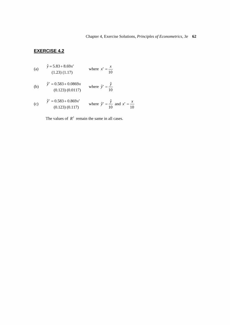
(a) Simple linear regression results:
( ) ( )
2
*** ***
ˆ 0.6776 0.0161 0.4595
(se) 0.0725 0.0026ty t R= + =
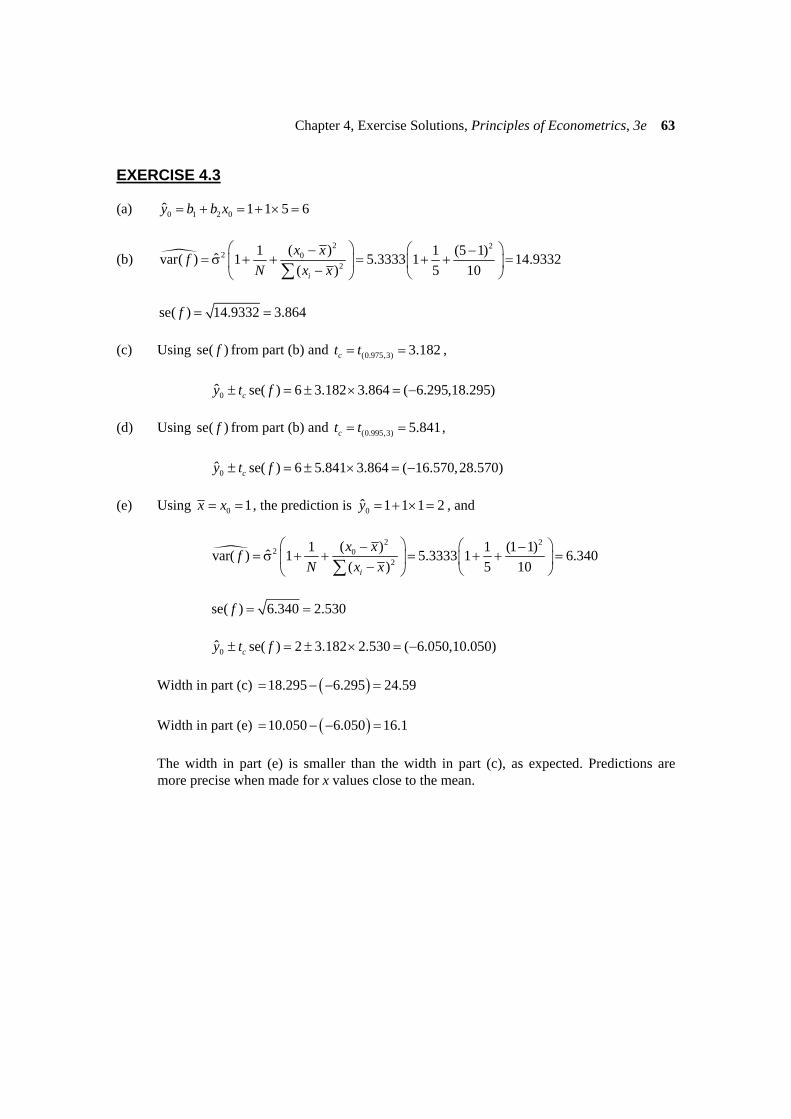
Linear-log regression results:
( )
( ) ( )
2
*** ***
ˆ 0.5287 0.1855 ln 0.2441
(se) 0.1472 0.0481ty t R= + =
Quadratic regression results:
( ) ( )
2 2
*** ***
ˆ 0.7914 0.000355 0.5685
(se) 0.0482 0.000046ty t R= + =
(b) (i) (ii)
-.8
-.4
.0
.4
.8
0.4
0.8
1.2
1.6
2.0
2.4
50 55 60 65 70 75 80 85 90 95
Residual Actual Fitted
Figure xr4.8(a) Fitted line and residuals for the simple linear regression
-0.8
-0.4
0.0
0.4
0.8
1.2
0.4
0.8
1.2
1.6
2.0
2.4
50 55 60 65 70 75 80 85 90 95
Residual Actual Fitted
Figure xr4.8(b) Fitted line and residuals for the linear-log regression
Chapter 4, Exercise Solutions, Principles of Econometrics, 3e 69
Exercise 4.8(b) continued
(b)
-.6
-.4
-.2
.0
.2
.4
.6
0.4
0.8
1.2
1.6
2.0
2.4
50 55 60 65 70 75 80 85 90 95
Residual Actual Fitted
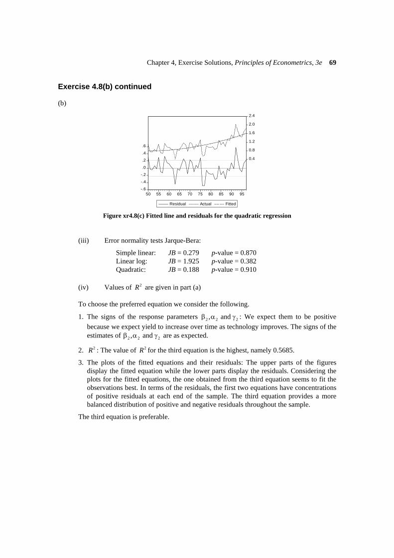
Figure xr4.8(c) Fitted line and residuals for the quadratic regression (iii) Error normality tests Jarque-Bera:
Simple linear: JB = 0.279 p-value = 0.870 Linear log: JB = 1.925 p-value = 0.382 Quadratic: JB = 0.188 p-value = 0.910 (iv) Values of 2R are given in part (a) To choose the preferred equation we consider the following.
1. The signs of the response parameters 2 2 2, and β α γ : We expect them to be positive because we expect yield to increase over time as technology improves. The signs of the estimates of 2 2 2, and β α γ are as expected.
2. 2R : The value of 2R for the third equation is the highest, namely 0.5685.
3. The plots of the fitted equations and their residuals: The upper parts of the figures display the fitted equation while the lower parts display the residuals. Considering the plots for the fitted equations, the one obtained from the third equation seems to fit the observations best. In terms of the residuals, the first two equations have concentrations of positive residuals at each end of the sample. The third equation provides a more balanced distribution of positive and negative residuals throughout the sample.
The third equation is preferable.
Chapter 4, Exercise Solutions, Principles of Econometrics, 3e 70
EXERCISE 4.9
(a) Equation 1: 0ˆ 0.6776 0.0161 49 1.467y = + × =
Equation 2: 0ˆ 0.5287 0.1855ln(49) 1.251y = + =
Equation 3: 20ˆ 0.7914 0.0003547 (49) 1.643y = + × =
(b) Equation 1: 1ˆ 0.0161tdy
dt= β =
Equation 2: 1ˆ 0.1855 0.003849
tdydt t
α= = =
Equation 3: 1ˆ2 2 0.0003547 49 0.0348tdy tdt
= γ = × × =
(c) Evaluating the elasticities at 49t = and the relevant value for 0y gives the following
results.
Equation 1: 10
49ˆ 0.0161 0.538ˆ 1.467
t
t
dy t tdt y y
= β = × =
Equation 2: 1ˆ 0.1855 0.148ˆ 1.251
t
t t
dy tdt y y
α= = =
Equation 3: 2 2
1
0
ˆ2 2 0.0003547 49 1.037ˆ 1.643
t
t
dy ttdt y y
γ × ×= = =
(d) The slopes tdydt
and the elasticities t
t
dy tdt y
give the marginal change in yield and the
percentage change in yield, respectively, that can be expected from technological change in the next year. The results show that the predicted effect of technological change is very sensitive to the choice of functional form.
Chapter 4, Exercise Solutions, Principles of Econometrics, 3e 71
EXERCISE 4.10
(a) For households with 1 child
2
1.0099 0.1495ln( )(se) (0.0401) (0.0090) 0.3203
( ) (25.19) ( 16.70)
WFOOD TOTEXPR
t
= −
=−
For households with 2 children:
2
0.9535 0.1294ln( )(se) (0.0365) (0.0080) 0.2206( ) (26.10) ( 16.16)
WFOOD TOTEXPR
t
= −
=−
For 2β we would expect a negative value because as the total expenditure increases the
food share should decrease with higher proportions of expenditure devoted to less essential items. Both estimations give the expected sign. The standard errors for 1 2 and b b from both estimations are relatively small resulting in high values of t ratios and significant estimates.
(b) For households with 1 child, the average total expenditure is 94.848 and
( )( )
[ ]1 2
1 2
ln 1 1.0099 0.1495 ln(94.848) 1ˆ 0.5461
1.0099 0.1495 ln(94.848)ln
b b TOTEXP
b b TOTEXP
⎡ ⎤+ + − × +⎣ ⎦η = = =− ×+
For households with 2 children, the average total expenditure is 101.168 and
( )( )
[ ]1 2
1 2
ln 1 0.9535 0.12944 ln(101.168) 1ˆ 0.6363
0.9535 0.12944 ln(101.168)ln
b b TOTEXP
b b TOTEXP
⎡ ⎤+ + − × +⎣ ⎦η = = =− ×+
Both of the elasticities are less than one; therefore, food is a necessity.
Chapter 4, Exercise Solutions, Principles of Econometrics, 3e 72
Exercise 4.10 (continued)
0.0
0.2
0.4
0.6
0.8
3 4 5 6
X1
WFO
OD
1
-0.4
-0.2
0.0
0.2
0.4
3 4 5 6
X1
RES
ID
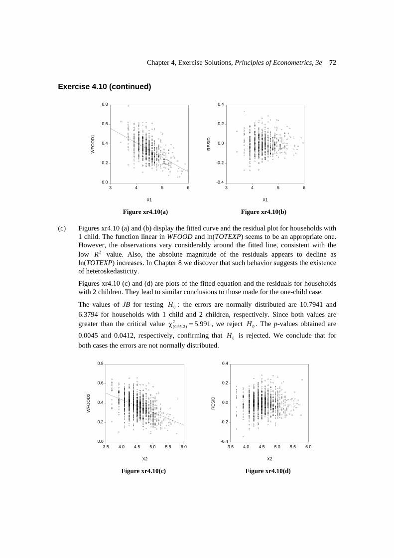
Figure xr4.10(a) Figure xr4.10(b) (c) Figures xr4.10 (a) and (b) display the fitted curve and the residual plot for households with
1 child. The function linear in WFOOD and ln(TOTEXP) seems to be an appropriate one. However, the observations vary considerably around the fitted line, consistent with the low 2R value. Also, the absolute magnitude of the residuals appears to decline as ln(TOTEXP) increases. In Chapter 8 we discover that such behavior suggests the existence of heteroskedasticity.
Figures xr4.10 (c) and (d) are plots of the fitted equation and the residuals for households with 2 children. They lead to similar conclusions to those made for the one-child case.
The values of JB for testing 0 :H the errors are normally distributed are 10.7941 and 6.3794 for households with 1 child and 2 children, respectively. Since both values are greater than the critical value 2
(0.95,2) 5.991χ = , we reject 0H . The p-values obtained are
0.0045 and 0.0412, respectively, confirming that 0H is rejected. We conclude that for both cases the errors are not normally distributed.
0.0
0.2
0.4
0.6
0.8
3.5 4.0 4.5 5.0 5.5 6.0
X2
WFO
OD
2
-0.4
-0.2
0.0
0.2
0.4
3.5 4.0 4.5 5.0 5.5 6.0
X2
RES
ID
Figure xr4.10(c) Figure xr4.10(d)
Chapter 4, Exercise Solutions, Principles of Econometrics, 3e 73
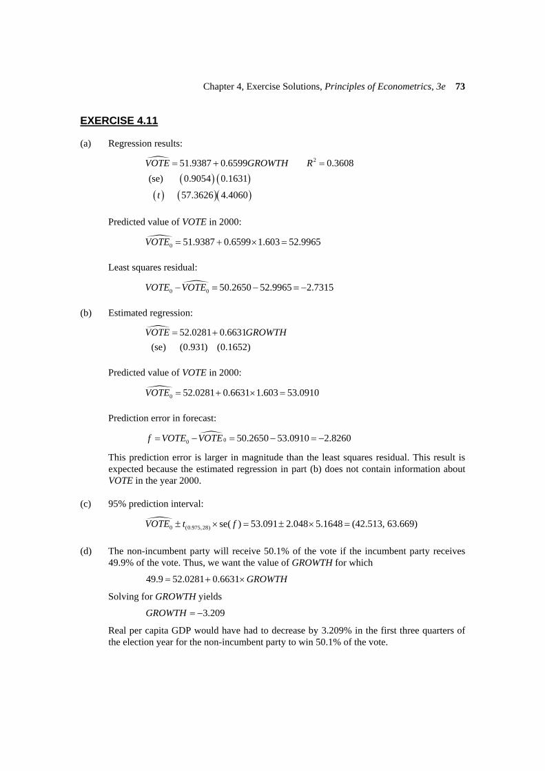
EXERCISE 4.11
(a) Regression results:
( ) ( )( ) ( )( )
251.9387 0.6599 0.3608(se) 0.9054 0.1631
57.3626 4.4060
VOTE GROWTH R
t
= + =
Predicted value of VOTE in 2000:
0 51.9387 0.6599 1.603 52.9965VOTE = + × = Least squares residual:
0 0 50.2650 52.9965 2.7315VOTE VOTE− = − = − (b) Estimated regression:
52.0281 0.6631(se) (0.931) (0.1652)
VOTE GROWTH= +
Predicted value of VOTE in 2000:
0 52.0281 0.6631 1.603 53.0910VOTE = + × = Prediction error in forecast:
00 50.2650 53.0910 2.8260f VOTE VOTE= − = − = −
This prediction error is larger in magnitude than the least squares residual. This result is expected because the estimated regression in part (b) does not contain information about VOTE in the year 2000.
(c) 95% prediction interval:
0 (0.975,28) se( ) 53.091 2.048 5.1648VOTE t f± × = ± × = (42.513, 63.669) (d) The non-incumbent party will receive 50.1% of the vote if the incumbent party receives
49.9% of the vote. Thus, we want the value of GROWTH for which
49.9 52.0281 0.6631 GROWTH= + ×
Solving for GROWTH yields
3.209GROWTH = −
Real per capita GDP would have had to decrease by 3.209% in the first three quarters of the election year for the non-incumbent party to win 50.1% of the vote.
Chapter 4, Exercise Solutions, Principles of Econometrics, 3e 74
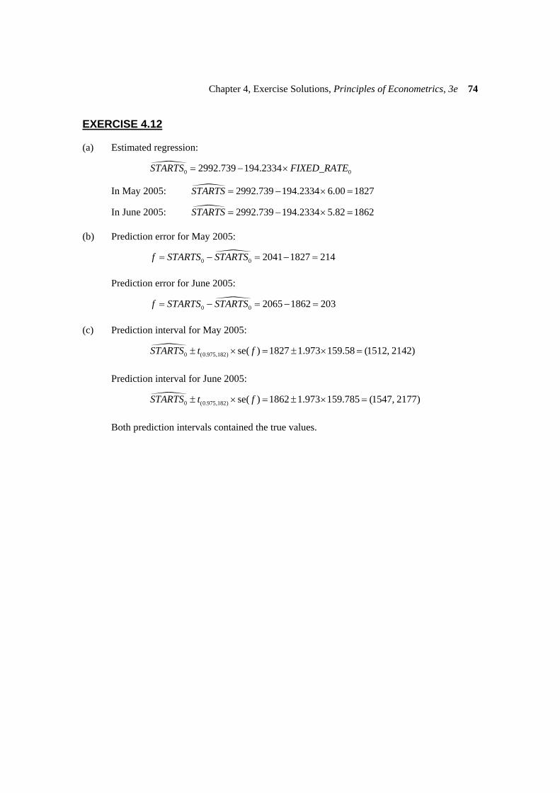
EXERCISE 4.12
(a) Estimated regression:
0 02992.739 194.2334STARTS FIXED_RATE= − ×
In May 2005: 2992.739 194.2334 6.00 1827STARTS = − × =
In June 2005: 2992.739 194.2334 5.82 1862STARTS = − × = (b) Prediction error for May 2005:
0 0 2041 1827 214f STARTS STARTS= − = − = Prediction error for June 2005:
0 0 2065 1862 203f STARTS STARTS= − = − = (c) Prediction interval for May 2005:
0 (0.975,182) se( ) 1827 1.973 159.58 (1512, 2142)STARTS t f± × = ± × = Prediction interval for June 2005:
0 (0.975,182) se( ) 1862 1.973 159.785 (1547, 2177)STARTS t f± × = ± × = Both prediction intervals contained the true values.
Chapter 4, Exercise Solutions, Principles of Econometrics, 3e 75
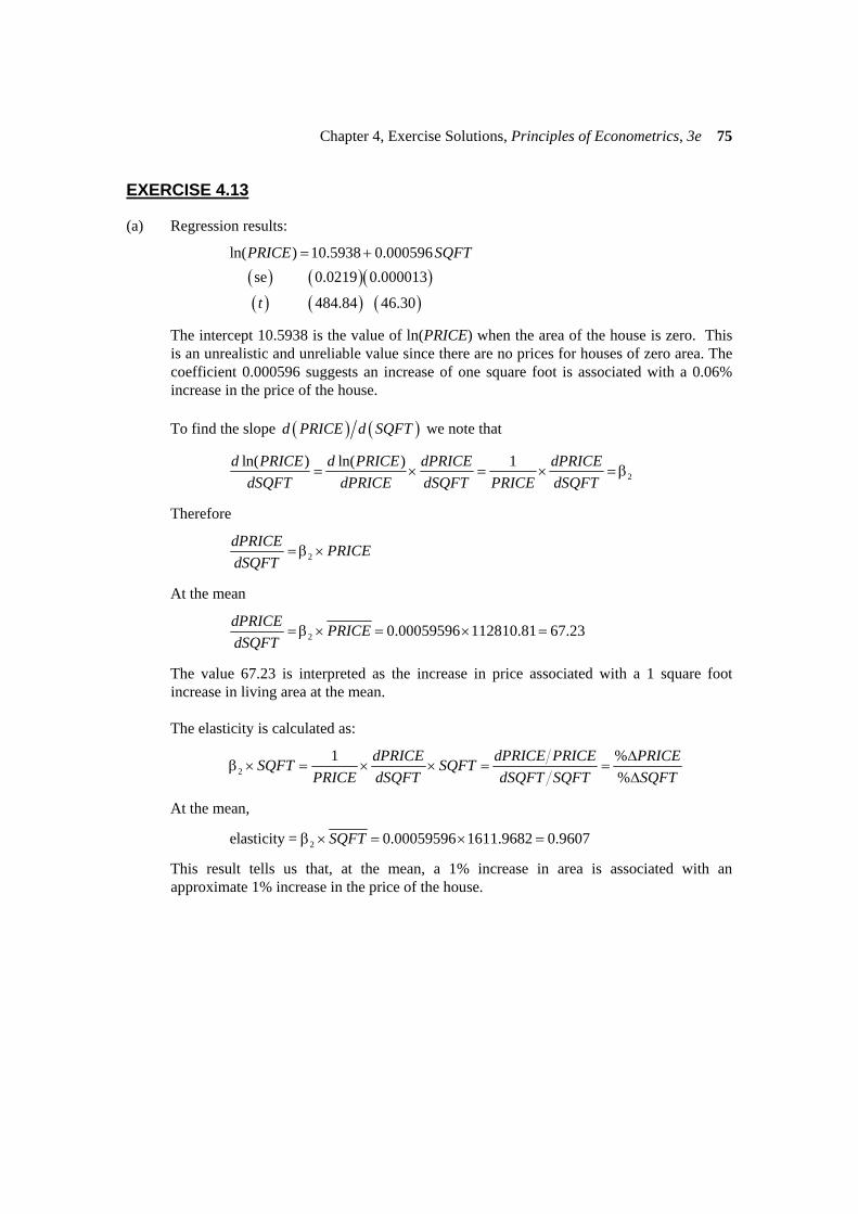
EXERCISE 4.13
(a) Regression results:
( ) ( )( )( ) ( ) ( )
ln( ) 10.5938 0.000596se 0.0219 0.000013
484.84 46.30
PRICE SQFT
t
= +
The intercept 10.5938 is the value of ln(PRICE) when the area of the house is zero. This is an unrealistic and unreliable value since there are no prices for houses of zero area. The coefficient 0.000596 suggests an increase of one square foot is associated with a 0.06% increase in the price of the house.
To find the slope ( ) ( )d PRICE d SQFT we note that
2ln( ) ln( ) 1d PRICE d PRICE dPRICE dPRICEdSQFT dPRICE dSQFT PRICE dSQFT
= × = × = β
Therefore
2dPRICE PRICEdSQFT
= β ×
At the mean
2 0.00059596 112810.81 67.23dPRICE PRICEdSQFT
= β × = × =
The value 67.23 is interpreted as the increase in price associated with a 1 square foot increase in living area at the mean.
The elasticity is calculated as:
21 %
%dPRICE dPRICE PRICE PRICESQFT SQFT
PRICE dSQFT dSQFT SQFT SQFTΔ
β × = × × = =Δ
At the mean,
2elasticity = 0.00059596 1611.9682 0.9607SQFTβ × = × =
This result tells us that, at the mean, a 1% increase in area is associated with an approximate 1% increase in the price of the house.

Chapter 4, Exercise Solutions, Principles of Econometrics, 3e 76
Exercise 4.13 (continued)
(b) Regression results:
( ) ( ) ( )( ) ( ) ( )
ln( ) 4.1707 1.0066ln( )se 0.1655 0.0225
25.20 44.65
PRICE SQFT
t
= +
The intercept 4.1707 is the value of ln(PRICE) when the area of the house is 1 square foot. This is an unrealistic and unreliable value since there are no prices for houses of 1 square foot in area. The coefficient 1.0066 says that an increase in living area of 1% is associated with a 1% increase in house price.
The coefficient 1.0066 is the elasticity since it is a constant elasticity functional form. To find the slope ( ) ( )d PRICE d SQFT note that
2ln( )ln( )
d PRICE SQFT dPRICEd SQFT PRICE dSQFT
= = β
Therefore,
2dPRICE PRICEdSQFT SQFT
= β ×
At the means,
2112810.811.0066 70.4441611.9682
dPRICE PRICEdSQFT SQFT
= β × = × =
The value 70.444 is interpreted as the increase in price associated by a 1 square foot increase in living area at the mean.
(c) From the linear function, 2 0.672R = .
From the log-linear function in part(a),
[ ]22 9
2 29 9
1.99573 10ˆcov( , )ˆ[corr( , )] 0.715
ˆvar( ) var( ) 2.78614 10 1.99996 10g
y yR y y
y y
⎡ ⎤×⎣ ⎦= = = =× × ×
From the log-log function in part(b),
[ ]22 9
2 29 9
1.57631 10ˆcov( , )ˆ[corr( , )] 0.673
ˆvar( ) var( ) 2.78614 10 1.32604 10g
y yR y y
y y
⎡ ⎤×⎣ ⎦= = = =× × ×
The highest 2R value is that of the log-linear functional form. The linear association between the data and the fitted line is highest for the log-linear functional form. In this sense the log-linear model fits the data best.

Chapter 4, Exercise Solutions, Principles of Econometrics, 3e 77
Exercise 4.13 (continued)
(d)
0
20
40
60
80
100
120
-0.75 -0.50 -0.25 0.00 0.25 0.50 0.75 Figure xr4.13(a) Histogram of residuals for log-linear model
0
20
40
60
80
100
120
-0.75 -0.50 -0.25 0.00 0.25 0.50 0.75 Figure xr4.13(b) Histogram of residuals for log-log model
0
40
80
120
160
200
-100000 0 100000 200000
Figure xr4.13(c) Histogram of residuals for simple linear model Log-linear: Jarque-Bera = 78.85, p -value = 0.0000 Log-Log: Jarque-Bera = 52.74, p -value = 0.0000 Simple linear: Jarque-Bera = 2456, p -value = 0.0000
All Jarque-Bera values are significantly different from 0 at the 1% level of significance. We can conclude that the residuals are not normally distributed.

Chapter 4, Exercise Solutions, Principles of Econometrics, 3e 78
Exercise 4.13 (continued)
(e)
-0.8
-0.4
0.0
0.4
0.8
1.2
0 1000 2000 3000 4000 5000
SQFT
resi
dual
Figure xr4.13(d) Residuals of log-linear model
-0.8
-0.4
0.0
0.4
0.8
1.2
0 1000 2000 3000 4000 5000
SQFT
resi
dual
Figure xr4.13(e) Residuals of log-log model
-150000
-100000
-50000
0
50000
100000
150000
200000
250000
0 1000 2000 3000 4000 5000
SQFT
resi
daul
Figure xr4.13(f) Residuals of simple linear model
The residuals appear to increase in magnitude as SQFT increases. This is most evident in
the residuals of the simple linear functional form. Furthermore, the residuals in the area around 1000 square feet of the simple linear model are all positive indicating that perhaps the functional form does not fit well in this region.
Chapter 4, Exercise Solutions, Principles of Econometrics, 3e 79
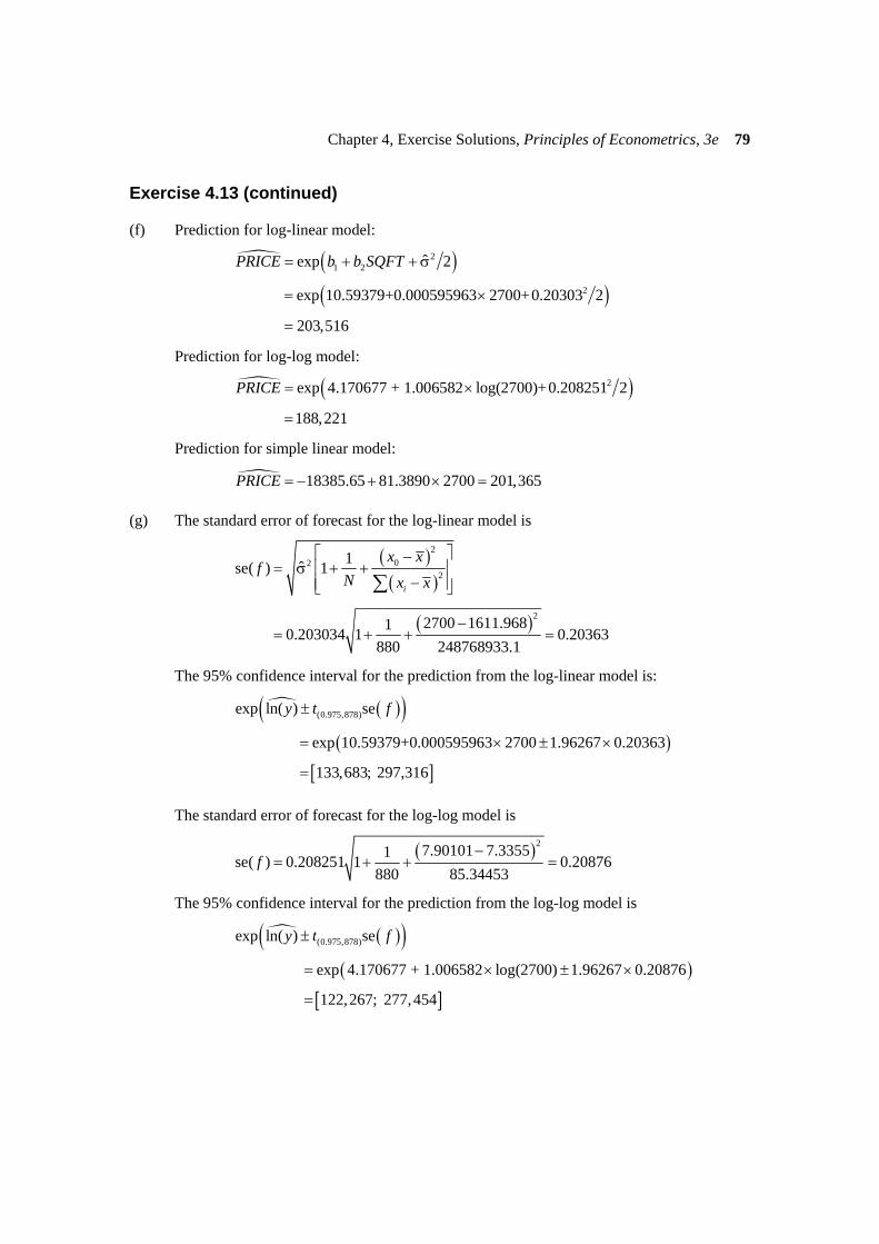
Exercise 4.13 (continued)
(f) Prediction for log-linear model:
( )( )
21 2
2
ˆexp 2
exp 10.59379+0.000595963 2700+0.20303 2
203,516
PRICE b b SQFT= + + σ
= ×
=
Prediction for log-log model:
( )2exp 4.170677 + 1.006582 log(2700)+0.208251 2
188,221
PRICE = ×
=
Prediction for simple linear model:
18385.65 81.3890 2700 201,365PRICE = − + × = (g) The standard error of forecast for the log-linear model is
( )( )
( )
202
2
2
1ˆse( ) 1
2700 1611.96810.203034 1 0.20363880 248768933.1
i
x xf
N x x
⎡ ⎤−= σ + +⎢ ⎥
−⎢ ⎥⎣ ⎦
−= + + =
∑
The 95% confidence interval for the prediction from the log-linear model is:
( )( )( )
[ ]
(0.975,878)exp ln( ) se
exp 10.59379+0.000595963 2700 1.96267 0.20363
133,683; 297,316
y t f±
= × ± ×
=
The standard error of forecast for the log-log model is
( )27.90101 7.33551se( ) 0.208251 1 0.20876880 85.34453
f−
= + + =
The 95% confidence interval for the prediction from the log-log model is
( )( )( )
[ ]
(0.975,878)exp ln( ) se
exp 4.170677 + 1.006582 log(2700) 1.96267 0.20876
122,267; 277,454
y t f±
= × ± ×
=
Chapter 4, Exercise Solutions, Principles of Econometrics, 3e 80
Exercise 4.13(g) (continued)
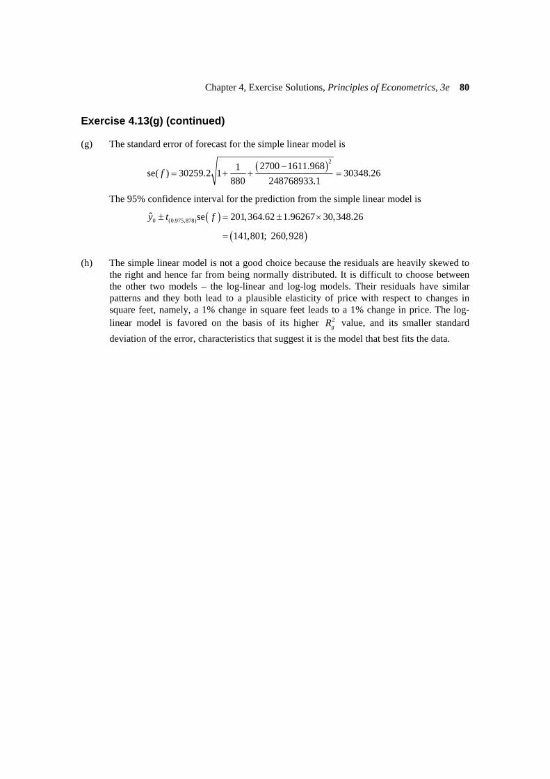
(g) The standard error of forecast for the simple linear model is
( )22700 1611.9681se( ) 30259.2 1 30348.26880 248768933.1
f−
= + + =
The 95% confidence interval for the prediction from the simple linear model is
( )
( )0 (0.975,878)ˆ se 201,364.62 1.96267 30,348.26
141,801; 260,928
y t f± = ± ×
=
(h) The simple linear model is not a good choice because the residuals are heavily skewed to
the right and hence far from being normally distributed. It is difficult to choose between the other two models – the log-linear and log-log models. Their residuals have similar patterns and they both lead to a plausible elasticity of price with respect to changes in square feet, namely, a 1% change in square feet leads to a 1% change in price. The log-linear model is favored on the basis of its higher 2
gR value, and its smaller standard deviation of the error, characteristics that suggest it is the model that best fits the data.

Chapter 4, Exercise Solutions, Principles of Econometrics, 3e 81
EXERCISE 4.14
(a)
0
40
80
120
160
200
240
0 10 20 30 40 50 60 Figure xr4.14(a) Histogram of WAGE
0
10
20
30
40
50
60
70
80
1.0 1.5 2.0 2.5 3.0 3.5 4.0 Figure xr4.14(b) Histogram of ln(WAGE)
Neither WAGE nor ln(WAGE) appear normally distributed. The distribution for WAGE is
positively skewed and that for ln(WAGE) is too flat at the top. However, ln(WAGE) more closely resembles a normal distribution. This conclusion is confirmed by the Jarque-Bera test results which are 2684JB = (p-value = 0.0000) for WAGE and 17.6JB = (p-value = 0.0002) for ln(WAGE).
(b) The regression results for the linear model are
( ) ( ) ( )
24.9122 1.1385 0.2024se 0.9668 0.0716
WAGE EDUC R= − + =
The estimated return to education at the mean 2 1.1385100 100 11.15%10.2130
bWAGE
= × = × =
The results for the log-linear model are
( )( ) ( ) ( )
2ln 0.7884 0.1038 0.2146
se 0.0849 0.0063
WAGE EDUC R= + =
The estimated return to education 2 100 10.38%.b= × =

Chapter 4, Exercise Solutions, Principles of Econometrics, 3e 82
Exercise 4.14 (continued)
(c)
0
40
80
120
160
200
240
-10 0 10 20 30 40
Figure xr4.14(c) Histogram of residuals from simple linear regression
0
10
20
30
40
50
60
70
80
90
-1.5 -1.0 -0.5 0.0 0.5 1.0 1.5
Figure xr4.14(d) Histogram of residuals from log-linear regression The Jarque-Bera test results are 3023JB = (p-value = 0.0000) for the residuals from the
linear model and 3.48JB = (p-value = 0.1754) for the residuals from the log-linear model.
Both the histograms and the Jarque-Bera test results suggest the residuals from the log-linear model are more compatible with normality. In the log-linear model a null hypothesis of normality is not rejected at a 10% level of significance. In the linear regression model it is rejected at a 1% level of significance.
(d) Linear model: 2 0.2024R =
Log-linear model:
[ ]2 22 2 ˆcov( , ) 6.87196ˆ[corr( , )] 0.2246
ˆvar( ) var( ) 38.9815 5.39435g
y yR y y
y y= = = =
×
Since, 2 2gR R> we conclude that the log-linear model fits the data better.

Chapter 4, Exercise Solutions, Principles of Econometrics, 3e 83
Exercise 4.14 (continued)
(e)
-20
-10
0
10
20
30
40
50
0 2 4 6 8 10 12 14 16 18 20
EDUC
resi
dual
Figure xr4.14(e) Residuals of the simple linear model
-1.6
-1.2
-0.8
-0.4
0.0
0.4
0.8
1.2
1.6
2.0
0 2 4 6 8 10 12 14 16 18 20
EDUC
resi
dual
Figure xr4.14(f) Residuals of the log-linear model
The absolute value of the residuals increases in magnitude as EDUC increases, suggesting
heteroskedasticity which is covered in Chapter 8. It is also apparent, for both models, that there are only positive residuals in the early range of EDUC. This suggests that there might be a threshold effect – education has an impact only after a minimum number of years of education. We also observe the non-normality of the residuals in the linear model; the positive residuals tend to be greater in absolute magnitude than the negative residuals.
(f) Prediction for simple linear model:
0 4.9122 1.1385 16 13.30WAGE = − + × =
Prediction for log-linear model:
( )2exp 0.7884 0.1038 16 (0.4902 ) / 2 13.05cWAGE = + × + =
Actual average wage of all workers with 16 years of education = 13.30 (g) The log-linear function is preferred because it has a higher goodness-of-fit value and its
residuals are consistent with normality. However, when predicting the average age of workers with 16 years of education, the linear model had a smaller prediction error
Chapter 4, Exercise Solutions, Principles of Econometrics, 3e 84
EXERCISE 4.15
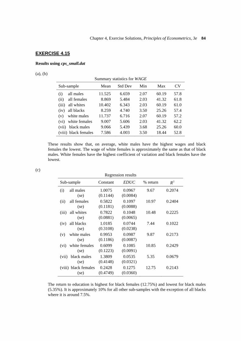
Results using cps_small.dat (a), (b)
Summary statistics for WAGE
Sub-sample Mean Std Dev Min Max CV
(i) all males 11.525 6.659 2.07 60.19 57.8 (ii) all females 8.869 5.484 2.03 41.32 61.8 (iii) all whites 10.402 6.343 2.03 60.19 61.0 (iv) all blacks 8.259 4.740 3.50 25.26 57.4 (v) white males 11.737 6.716 2.07 60.19 57.2 (vi) white females 9.007 5.606 2.03 41.32 62.2 (vii) black males 9.066 5.439 3.68 25.26 60.0 (viii) black females 7.586 4.003 3.50 18.44 52.8
These results show that, on average, white males have the highest wages and black
females the lowest. The wage of white females is approximately the same as that of black males. White females have the highest coefficient of variation and black females have the lowest.
(c)
Regression results
Sub-sample Constant EDUC % return 2R
(i) all males 1.0075 0.0967 9.67 0.2074 (se) (0.1144) (0.0084) (ii) all females 0.5822 0.1097 10.97 0.2404 (se) (0.1181) (0.0088) (iii) all whites 0.7822 0.1048 10.48 0.2225 (se) (0.0881) (0.0065) (iv) all blacks 1.0185 0.0744 7.44 0.1022 (se) (0.3108) (0.0238) (v) white males 0.9953 0.0987 9.87 0.2173 (se) (0.1186) (0.0087) (vi) white females 0.6099 0.1085 10.85 0.2429 (se) (0.1223) (0.0091) (vii) black males 1.3809 0.0535 5.35 0.0679 (se) (0.4148) (0.0321) (viii) black females 0.2428 0.1275 12.75 0.2143 (se) (0.4749) (0.0360)
The return to education is highest for black females (12.75%) and lowest for black males
(5.35%). It is approximately 10% for all other sub-samples with the exception of all blacks where it is around 7.5%.
Chapter 4, Exercise Solutions, Principles of Econometrics, 3e 85
Exercise 4.15 (continued)
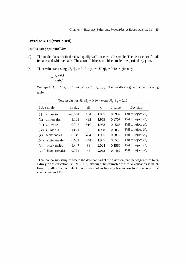
Results using cps_small.dat (d) The model does not fit the data equally well for each sub-sample. The best fits are for all
females and white females. Those for all blacks and black males are particularly poor. (e) The t-value for testing 0 2: 0.10H β = against 1 2: 0.10H β ≠ is given by
2
2
0.1se( )
btb−
=
We reject 0H if ct t> or ct t< − where (0.975,df )ct t= . The results are given in the following table.
Test results for 0 2: 0.10H β = versus 1 2: 0.10H β ≠
Sub-sample t-value df ct p-value Decision
(i) all males − 0.394 504 1.965 0.6937 Fail to reject 0H
(ii) all females 1.103 492 1.965 0.2707 Fail to reject 0H
(iii) all whites 0.745 910 1.963 0.4563 Fail to reject 0H
(iv) all blacks − 1.074 86 1.988 0.2856 Fail to reject 0H
(v) white males − 0.149 464 1.965 0.8817 Fail to reject 0H
(vi) white females 0.931 444 1.965 0.3525 Fail to reject 0H
(vii) black males − 1.447 38 2.024 0.1560 Fail to reject 0H
(viii) black females 0.764 46 2.013 0.4485 Fail to reject 0H
There are no sub-samples where the data contradict the assertion that the wage return to an
extra year of education is 10%. Thus, although the estimated return to education is much lower for all blacks and black males, it is not sufficiently less to conclude conclusively it is not equal to 10%.

Chapter 4, Exercise Solutions, Principles of Econometrics, 3e 86
EXERCISE 4.15
Results using cps.dat (a), (b)
Summary statistics for WAGE
Sub-sample Mean Std Dev Min Max CV
(i) all males 11.315 6.521 1.05 74.32 57.6 (ii) all females 8.990 5.630 1.28 78.71 62.6 (iii) all whites 10.358 6.275 1.05 78.71 60.6 (iv) all blacks 8.626 5.387 1.57 39.35 62.5 (v) white males 11.491 6.591 1.05 74.32 57.4 (vi) white females 9.105 5.648 1.28 78.71 62.0 (vii) black males 9.307 5.274 2.76 34.07 56.7 (viii) black females 8.129 5.424 1.57 39.35 66.7
These results show that, on average, white males have the highest wages and black
females the lowest. Males have higher average wages than females and whites have higher average wages than blacks. The highest wage earner is, however, a white female. Black females have the highest coefficient of variation and black males have the lowest.
(c)
Regression results
Sub-sample Constant EDUC % return 2R
(i) all males 0.9798 0.0982 9.82 0.1954 (se) (0.0543) (0.0040) (ii) all females 0.4776 0.1173 11.73 0.2479 (se) (0.0579) (0.0043) (iii) all whites 0.7965 0.1040 10.40 0.2030 (se) (0.0428) (0.0032) (iv) all blacks 0.6230 0.1066 10.66 0.1800 (se) (0.1390) (0.0106) (v) white males 0.9859 0.0988 9.88 0.2009 (se) (0.0561) (0.0042) (vi) white females 0.5142 0.1152 11.52 0.2453 (se) (0.0611) (0.0045) (vii) black males 1.0641 0.0798 7.98 0.1167 (se) (0.2063) (0.0157) (viii) black females 0.2147 0.1327 13.27 0.2569 (se) (0.1820) (0.0138)
The return to education is highest for black females (13.27%) and lowest for black males
(7.98%). It is approximately 10% for all other sub-samples with the exception of all females and white females where it is around 11.5%.
Chapter 4, Exercise Solutions, Principles of Econometrics, 3e 87
Exercise 4.15 (continued)
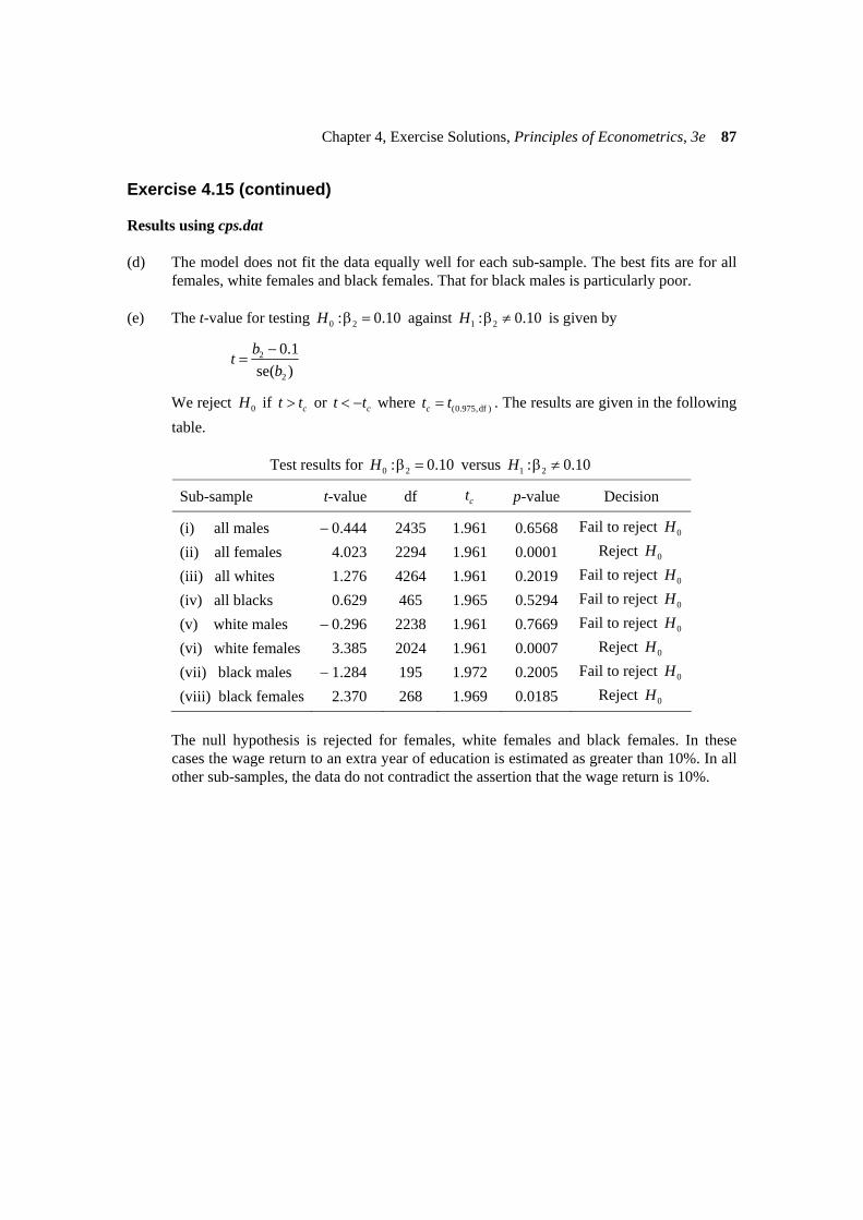
Results using cps.dat (d) The model does not fit the data equally well for each sub-sample. The best fits are for all
females, white females and black females. That for black males is particularly poor. (e) The t-value for testing 0 2: 0.10H β = against 1 2: 0.10H β ≠ is given by
2
2
0.1se( )
btb−
=
We reject 0H if ct t> or ct t< − where (0.975,df )ct t= . The results are given in the following table.
Test results for 0 2: 0.10H β = versus 1 2: 0.10H β ≠
Sub-sample t-value df ct p-value Decision
(i) all males − 0.444 2435 1.961 0.6568 Fail to reject 0H
(ii) all females 4.023 2294 1.961 0.0001 Reject 0H
(iii) all whites 1.276 4264 1.961 0.2019 Fail to reject 0H
(iv) all blacks 0.629 465 1.965 0.5294 Fail to reject 0H
(v) white males − 0.296 2238 1.961 0.7669 Fail to reject 0H
(vi) white females 3.385 2024 1.961 0.0007 Reject 0H
(vii) black males − 1.284 195 1.972 0.2005 Fail to reject 0H
(viii) black females 2.370 268 1.969 0.0185 Reject 0H
The null hypothesis is rejected for females, white females and black females. In these
cases the wage return to an extra year of education is estimated as greater than 10%. In all other sub-samples, the data do not contradict the assertion that the wage return is 10%.
Chapter 4, Exercise Solutions, Principles of Econometrics, 3e 88
EXERCISE 4.16
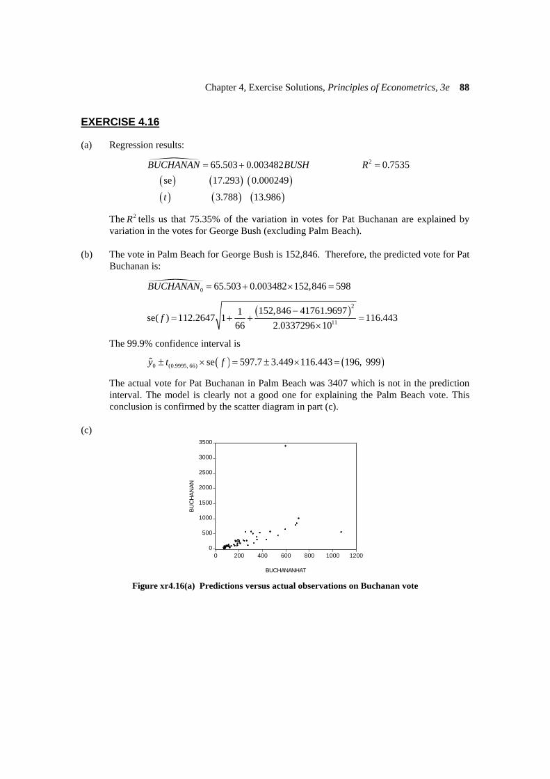
(a) Regression results:
( ) ( ) ( )( ) ( ) ( )
265.503 0.003482 0.7535se 17.293 0.000249
3.788 13.986
BUCHANAN BUSH R
t
= + =
The 2R tells us that 75.35% of the variation in votes for Pat Buchanan are explained by variation in the votes for George Bush (excluding Palm Beach).
(b) The vote in Palm Beach for George Bush is 152,846. Therefore, the predicted vote for Pat
Buchanan is:
0 65.503 0.003482 152,846 598BUCHANAN = + × =
( )2
11
152,846 41761.96971se( ) 112.2647 1 116.44366 2.0337296 10
f−
= + + =×
The 99.9% confidence interval is
( ) ( )0 (0.9995, 66)ˆ se 597.7 3.449 116.443 196, 999y t f± × = ± × =
The actual vote for Pat Buchanan in Palm Beach was 3407 which is not in the prediction interval. The model is clearly not a good one for explaining the Palm Beach vote. This conclusion is confirmed by the scatter diagram in part (c).
(c)
0
500
1000
1500
2000
2500
3000
3500
0 200 400 600 800 1000 1200
BUCHANANHAT
BUC
HAN
AN
Figure xr4.16(a) Predictions versus actual observations on Buchanan vote

Chapter 4, Exercise Solutions, Principles of Econometrics, 3e 89
Exercise 4.16 (continued)
(d) Regression results:
( ) ( ) ( )( ) ( ) ( )
2109.23 0.002544 0.6305se 19.52 0.000243
5.596 10.450
BUCHANAN GORE R
t
= + =
The 2R tells us that 63.05% of the variation in votes for Pat Buchanan are explained by variation in the votes for Al Gore (excluding Palm Beach).
The vote in Palm Beach for Al Gore is 268,945. Therefore, the predicted vote for Pat
Buchanan is:
0 109.23 0.002544 268945 793BUCHANAN = + × =
( )2
11
268,945 39975.551se( ) 137.4493 1 149.28166 3.188628 10
f−
= + + =×
The 99.9% confidence interval is
( ) ( )0 (0.9995, 66)ˆ se 793.3 3.449 149.281 278, 1308y t f± × = ± × =
The actual vote for Pat Buchanan in Palm Beach was 3407 which is not in the prediction interval. The model is clearly not a good one for explaining the Palm Beach vote. This conclusion is confirmed by the scatter diagram below.
0
500
1,000
1,500
2,000
2,500
3,000
3,500
0 200 400 600 800 1,000 1,200
BUCHANANHAT2
BUC
HAN
AN
Figure xr4.16(b) Predictions versus actual observations on Buchanan vote
Chapter 4, Exercise Solutions, Principles of Econometrics, 3e 90
Exercise 4.16 (continued)
(e) Regression results:
( ) ( ) ( )( ) ( ) ( )
20.0017 0.01142 0.1004se 0.0024 0.00427
0.710 2.673
BUCHSHARE BUSHSHARE R
t
= − + =
−
The share of votes for George Bush in Palm Beach was 0.354827. Therefore, the predicted share of votes in Palm Beach for Pat Buchanan is:
0 0.001706 0.011424 0.354827 0.002348BUCHSHARE = − + × =
The standard error of the forecast error is
( )20.354827 0.5547561se( ) 0.003078 1 0.003216866 0.518621
f−
= + + =
A 99.9% confidence interval is given by
( ) ( )0 (0.9995, 66)ˆ se 0.002349 3.449 0.0032168 0.0087457, 0.0134437y t f± × = ± × = −
There were 430,762 total votes cast in Palm Beach. Multiplying the confidence interval endpoints by this figure yields ( )3767, 5791− . The actual vote for Pat Buchanan in Palm Beach was 3407 which falls inside this interval.