2-1

Solutions for Chapter 2 Problems 1. Vectors in the Cartesian Coordinate System P2.1: Given P(4,2,1) and APQ=2ax +4ay +6az, find the point Q. APQ = 2 ax + 4 ay + 6 az = (Qx-Px)ax + (Qy-Py)ay+(Qz-Pz)azQx-Px=Qx-4=2; Qx=6 Qy-Py=Qy-2=4; Qy=6 Qz-Pz=Qz-1=6; Qz=7 Ans: Q(6,6,7) P2.2: Given the points P(4,1,0)m and Q(1,3,0)m, fill in the table and make a sketch of the vectors found in (a) through (f). Vector Mag Unit Vector a. Find the vector A from the origin to P

AOP = 4 ax + 1 ay 4.12 AOP = 0.97 ax + 0.24 ay

b. Find the vector B from the origin to Q

BOQ = 1 ax + 3 ay 3.16 aOQ = 0.32 ax + 0.95 ay

c. Find the vector C from P to Q

CPQ = -3 ax + 2 ay 3.61 aPQ = -0.83 ax + 0.55 ay

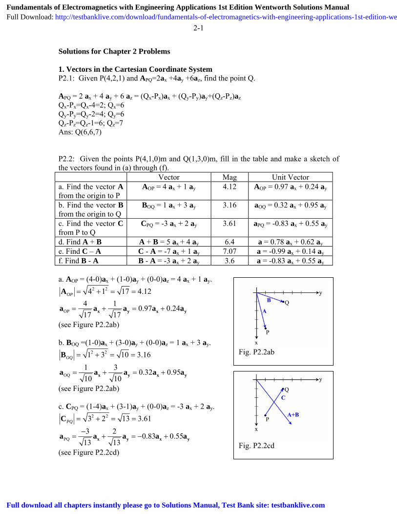
d. Find A + B A + B = 5 ax + 4 ay 6.4 a = 0.78 ax + 0.62 aye. Find C – A C - A = -7 ax + 1 ay 7.07 a = -0.99 ax + 0.14 ayf. Find B - A B - A = -3 ax + 2 ay 3.6 a = -0.83 ax + 0.55 ay a. AOP = (4-0)ax + (1-0)ay + (0-0)az = 4 ax + 1 ay.

Fig. P2.2ab

2 24 1 17 4.12OP = + = =A

OP4 1 0.97 0.2417 17

= + = +x y xa a a a ya

(see Figure P2.2ab) b. BOQ =(1-0)ax + (3-0)ay + (0-0)az = 1 ax + 3 ay.

2 21 3 10 3.16OQ = + = =B

OQ1 3 0.32 0.9510 10

= + = +x y xa a a a ya

Fig. P2.2cd

(see Figure P2.2ab) c. CPQ = (1-4)ax + (3-1)ay + (0-0)az = -3 ax + 2 ay.

2 23 2 13 3.61PQ = + = =C

PQ3 2 0.83 0.55

13 13−

= + = − +x y xa a a a ya

(see Figure P2.2cd)

Fundamentals of Electromagnetics with Engineering Applications 1st Edition Wentworth Solutions ManualFull Download: http://testbanklive.com/download/fundamentals-of-electromagnetics-with-engineering-applications-1st-edition-wentworth-solutions-manual/

Full download all chapters instantly please go to Solutions Manual, Test Bank site: testbanklive.com

2-2

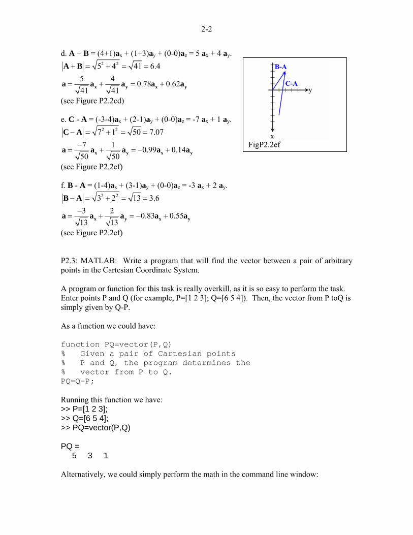
d. A + B = (4+1)ax + (1+3)ay + (0-0)az = 5 ax + 4 ay.

FigP2.2ef

2 25 4 41 6.4+ = + = =A B 5 4 0.78 0.6241 41

= + = +x y xa a a a ya

(see Figure P2.2cd) e. C - A = (-3-4)ax + (2-1)ay + (0-0)az = -7 ax + 1 ay.

2 27 1 50 7.07− = + = =C A 7 1 0.99 0.1450 50

−= + = − +x y xa a a a ya

(see Figure P2.2ef) f. B - A = (1-4)ax + (3-1)ay + (0-0)az = -3 ax + 2 ay.

2 23 2 13 3.6− = + = =B A 3 2 0.83 0.55

13 13−

= + = − +x y xa a a a ya

(see Figure P2.2ef) P2.3: MATLAB: Write a program that will find the vector between a pair of arbitrary points in the Cartesian Coordinate System. A program or function for this task is really overkill, as it is so easy to perform the task. Enter points P and Q (for example, P=[1 2 3]; Q=[6 5 4]). Then, the vector from P toQ is simply given by Q-P. As a function we could have: function PQ=vector(P,Q) % Given a pair of Cartesian points % P and Q, the program determines the % vector from P to Q. PQ=Q-P; Running this function we have: >> P=[1 2 3]; >> Q=[6 5 4]; >> PQ=vector(P,Q) PQ = 5 3 1 Alternatively, we could simply perform the math in the command line window:

2-3

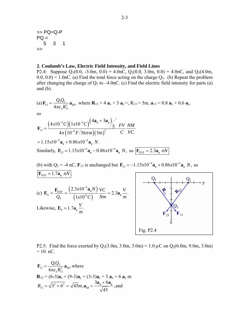
>> PQ=Q-P PQ = 5 3 1 >> 2. Coulomb’s Law, Electric Field Intensity, and Field Lines P2.4: Suppose Q1(0.0, -3.0m, 0.0) = 4.0nC, Q2(0.0, 3.0m, 0.0) = 4.0nC, and Q3(4.0m, 0.0, 0.0) = 1.0nC. (a) Find the total force acting on the charge Q3. (b) Repeat the problem after changing the charge of Q2 to –4.0nC. (c) Find the electric field intensity for parts (a) and (b).

(a) 1 213 2

13

,4 o

Q QRπε

= 13F a where R13 = 4 ax + 3 ay =, R13 = 5m, a13 = 0.8 ax + 0.6 ay.

so

( ) ( ) ( )

( ) ( )

9 9

13 29

9 9

4 34 10 1 10 5

4 10 36 5

1.15 10 0.86 10 .

x C x C FV NMC VCF m m

x x N

π π

− −

−

− −

+

=

= +

x y

x y

a aF

a a

Similarly, 9 923 1.15 10 0.86 10 ,x x N− −= −x yF a a so 2.3 TOT nN= xF a

(b) with Q2 = -4 nC, F13 is unchanged but 9 9

23 1.15 10 0.86 10 ,x x N− −= − +x yF a a so

1.7 .TOT nN= yF a

(c) ( )

( )9

-93

2.3 102.3 .

1 10TOT

a

x N VC VQ Nm mx C

−

= = =xx

aFE a

Fig. P2.4

Likewise, 1.7 .bVm

= yE a

P2.5: Find the force exerted by Q1(3.0m, 3.0m, 3.0m) = 1.0 µC on Q2(6.0m, 9.0m, 3.0m) = 10. nC.

1 212 2

12

, where4 o

Q QRπε

= 12F a

R12 = (6-3)ax + (9-3)ay + (3-3)az = 3 ax + 6 ay m 2 2

12

3 63 6 45 , ,and

45R m

+= + = = x y

12

a aa

2-4

( ) ( )( ) ( )

6 9

12 9 2

1 10 10 10 3 610 454 4536

x C x C FV NMC VCF mmπ π

− −

−

+= x ya a

F , so 12 0.89 1.8 .Nµ= +x yF a a

Fig. P2.5

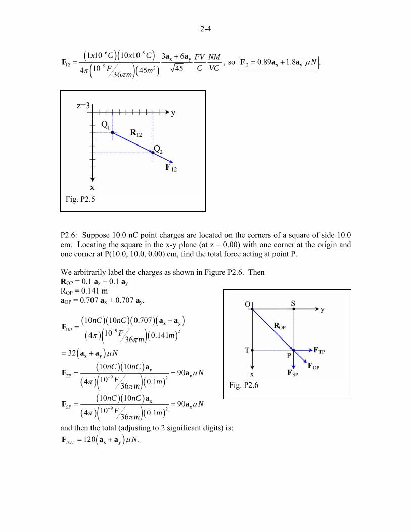
P2.6: Suppose 10.0 nC point charges are located on the corners of a square of side 10.0 cm. Locating the square in the x-y plane (at z = 0.00) with one corner at the origin and one corner at P(10.0, 10.0, 0.00) cm, find the total force acting at point P. We arbitrarily label the charges as shown in Figure P2.6. Then ROP = 0.1 ax + 0.1 ayROP = 0.141 m aOP = 0.707 ax + 0.707 ay.

( ) ( ) ( )( )( )( ) ( )

( )

9 2

10 10 0.707104 0.14136

32

OP

nC nCF mm

N

π π

µ

−

+=

= +

x y

x y

a aF

a a

( )( )( )( )( )9 2

10 1090

104 0.136TP

nC nCN

F mmµ

π π−

= =yy

aF a

( )( )( )( )( )9 2

10 1090

104 0.136SP

nC nCN

F mmµ

π π−

= =xx

aF a

Fig. P2.6

and then the total (adjusting to 2 significant digits) is: ( )120 .TOT Nµ= +x yF a a

2-5

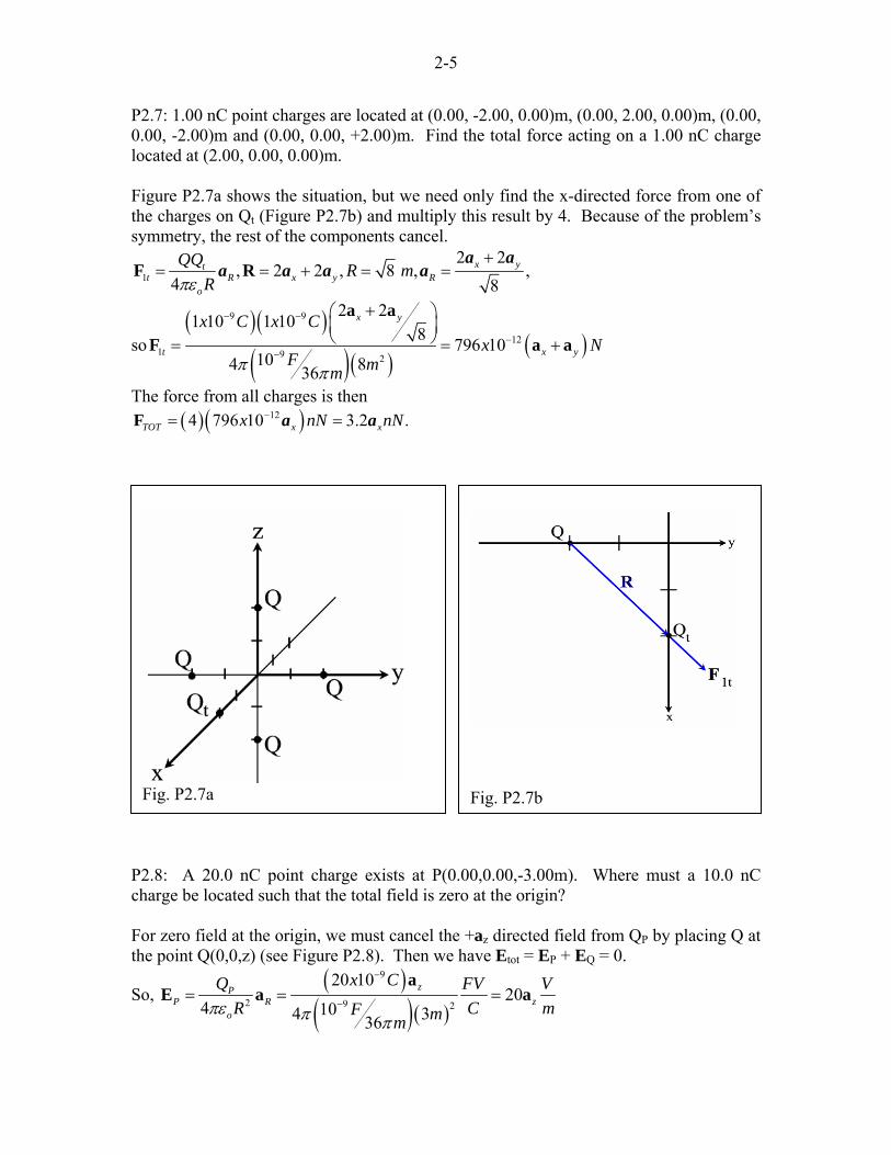
P2.7: 1.00 nC point charges are located at (0.00, -2.00, 0.00)m, (0.00, 2.00, 0.00)m, (0.00, 0.00, -2.00)m and (0.00, 0.00, +2.00)m. Find the total force acting on a 1.00 nC charge located at (2.00, 0.00, 0.00)m. Figure P2.7a shows the situation, but we need only find the x-directed force from one of the charges on Qt (Figure P2.7b) and multiply this result by 4. Because of the problem’s symmetry, the rest of the components cancel.

1

2 2, 2 2 , 8 ,

4 8x yt

t R x y Ro

QQ R mRπε

,+

= = + = =F Ra a

a a a a

so( )( )

( )( )( )

9 9

121 9 2

2 21 10 1 108 796 10

104 836

x y

t x y

x C x Cx N

F mmπ π

− −

−−

+⎛ ⎞⎜ ⎟⎝ ⎠= =

a a

F a + a

The force from all charges is then ( )( )124 796 10 3.2 .TOT x xx nN nN−= =F a a

Fig. P2.7a

Fig. P2.7b

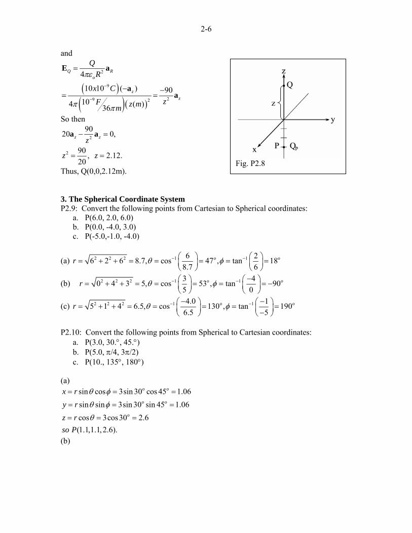
P2.8: A 20.0 nC point charge exists at P(0.00,0.00,-3.00m). Where must a 10.0 nC charge be located such that the total field is zero at the origin? For zero field at the origin, we must cancel the +az directed field from QP by placing Q at the point Q(0,0,z) (see Figure P2.8). Then we have Etot = EP + EQ = 0.

So, ( )

( )( )

9

2 9 2

20 1020

4 104 336

zPP R

o

x CQ FV VzR C mF mm

πε π π

−

−= = =

aE a a

2-6

and

Fig. P2.8

( )( )( )

2

9

29 2

4

10 10 ( ) 90104 ( )36

Q Ro

zz

QR

x CzF z mm

πε

π π

−

−

=

− −= =

E a

aa

So then

2

2

9020 0,

90 , 2.12.20

z zz

z z

− =

= =

a a

Thus, Q(0,0,2.12m). 3. The Spherical Coordinate System P2.9: Convert the following points from Cartesian to Spherical coordinates:

a. P(6.0, 2.0, 6.0) b. P(0.0, -4.0, 3.0) c. P(-5.0,-1.0, -4.0)

(a) 2 2 2 1 16 26 2 6 8.7, cos 47 , tan 188.7 6

o or θ φ− −⎛ ⎞ ⎛ ⎞= + + = = = = =⎜ ⎟ ⎜ ⎟⎝ ⎠ ⎝ ⎠

(b) 2 2 2 1 13 40 4 3 5, cos 53 , tan 905 0

o or θ φ− − −⎛ ⎞ ⎛ ⎞= + + = = = = = −⎜ ⎟ ⎜ ⎟⎝ ⎠ ⎝ ⎠

(c) 2 2 2 1 14.0 15 1 4 6.5, cos 130 , tan 1906.5 5

o or θ φ− −− −⎛ ⎞ ⎛ ⎞= + + = = = = =⎜ ⎟ ⎜ ⎟−⎝ ⎠ ⎝ ⎠

P2.10: Convert the following points from Spherical to Cartesian coordinates:

a. P(3.0, 30.°, 45.°) b. P(5.0, π/4, 3π/2) c. P(10., 135°, 180°)

(a)

sin cos 3sin 30 cos 45 1.06sin sin 3sin 30 sin 45 1.06cos 3cos30 2.6

(1.1,1.1, 2.6).

o o

o o

o

x ry rz rso P

θ φ

θ φ

θ

= = =

= = =

= = =

(b)

2-7

sin cos 5sin 45 cos 270 0sin sin 5sin 45 sin 270 3.5cos 5cos 45 3.5

(0, 3.5,3.5).

o o

o o

o

x ry rz rso P

θ φ

θ φ

θ

= =

= = =

= = =−

=

−

−

(c) sin cos 10sin135 cos180 7.1sin sin 10sin135 sin180 0cos 10cos135 7.1

( 7.1,0, 7.1).

o o

o o

o

x ry rz rso P

θ φ

θ φ

θ

= = =

= = =

= = = −− −

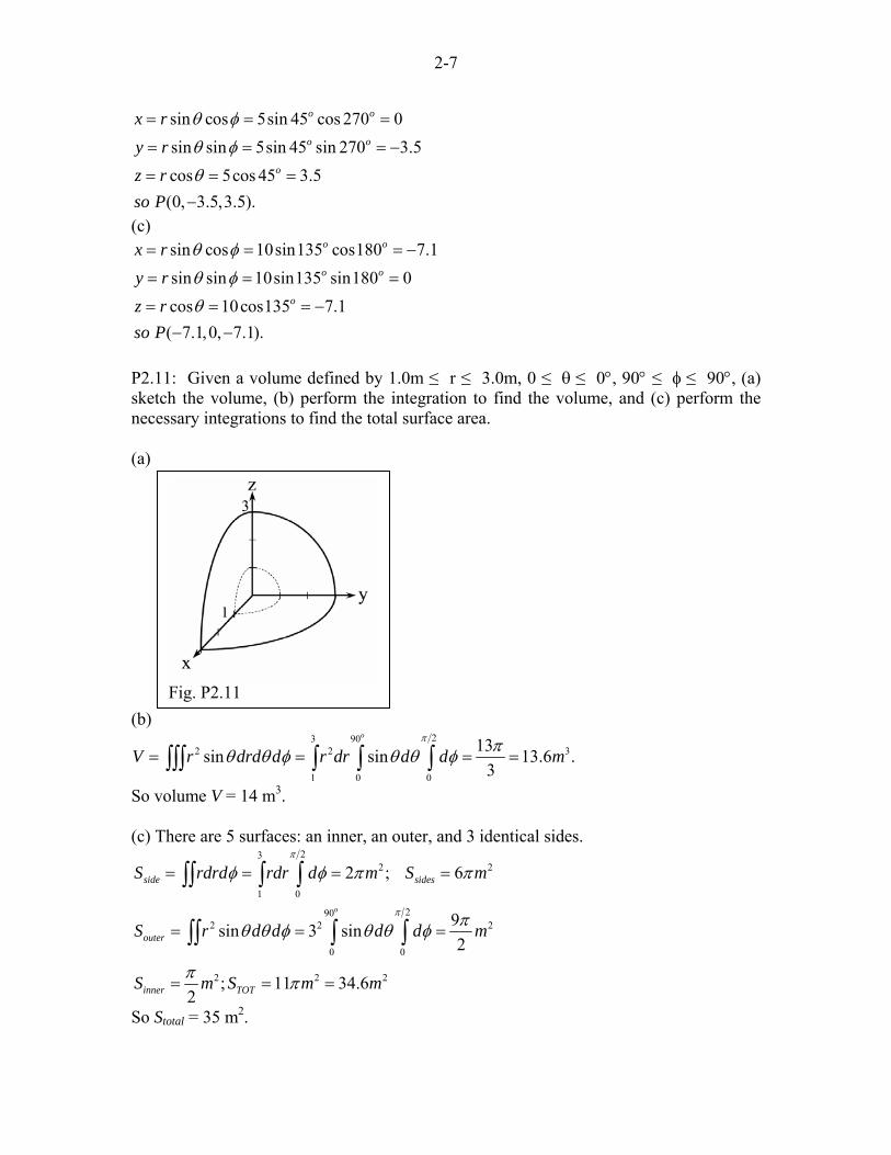
P2.11: Given a volume defined by 1.0m ≤ r ≤ 3.0m, 0 ≤ θ ≤ 0°, 90° ≤ φ ≤ 90°, (a) sketch the volume, (b) perform the integration to find the volume, and (c) perform the necessary integrations to find the total surface area. (a)

(b)

V =

So v (c) T

side

oute

inne

S

S

S

So S

Fig. P2.11

23 902 2

1 0 0

13sin sin 13.6 .3

o

r drd d r dr d d mπ πθ θ φ θ θ φ= =∫∫∫ ∫ ∫ ∫ 3=

olume V = 14 m3.

here are 5 surfaces: an inner, an outer, and 3 identical sides. 23

2 2

1 0

2902 2

0 0

2 2 2

2 ; 6

9sin 3 sin2

; 11 34.62

o

sides

r

r TOT

rdrd rdr d m S m

r d d d d

m S m m

π

π

φ φ π

πθ θ φ θ θ φ

π π

= = = =

= = =

= = =

∫∫ ∫ ∫

∫∫ ∫ ∫ 2m

π

total = 35 m2.

2-8

4. Line Charges and the Cylindrical Coordinate System P2.12: Convert the following points from Cartesian to cylindrical coordinates:

a. P(0.0, 4.0, 3.0) b. P(-2.0, 3.0, 2.0) c. P(4.0, -3.0, -4.0)

(a) 2 2 1 40 4 4, tan 90 , 3, (4.0,90 ,3.0)0

o oz so Pρ φ − ⎛ ⎞= + = = = =⎜ ⎟⎝ ⎠

(b) 2 2 1 32 3 3.6, tan 124 , 2, (3.6,120 , 2.0)2

o oz so Pρ φ − ⎛ ⎞= + = = = =⎜ ⎟−⎝ ⎠

(c) 2 2 1 34 3 5, tan 37 , 4, (5.0, 37 , 4.0)4

o oz so Pρ φ − −⎛ ⎞= + = = = − = − − −⎜ ⎟⎝ ⎠

P2.13: Convert the following points from cylindrical to Cartesian coordinates:

a. P(2.83, 45.0°, 2.00) b. P(6.00, 120.°, -3.00) c. P(10.0, -90.0°, 6.00)

(a)

cos 2.83cos 45 2.00sin 2.83sin 45 2.00

2.00 (2.00,2.00,2.00).

o

o

xyz zso P

ρ φ

ρ φ

= = =

= = == =

(b) cos 6.00cos120 3.00sin 6.00sin120 5.20

3.00 ( 3.00,5.20, 3.00).

o

o

xyz zso P

ρ φ

ρ φ

= = = −

= = == = −

− −

(c) cos 10.0cos( 90.0 ) 0sin 10.0sin( 90.0 ) 10.0

6.00 (0, 10.0,6.00).

o

o

xyz zso P

ρ φ

ρ φ

= = − =

= = − = −= =

−

P2.14: A 20.0 cm long section of copper pipe has a 1.00 cm thick wall and outer diameter of 6.00 cm.

a. Sketch the pipe conveniently overlaying the cylindrical coordinate system, lining up the length direction with the z-axis

b. Determine the total surface area (this could actually be useful if, say, you needed to do an electroplating step on this piece of pipe)

c. Determine the weight of the pipe given the density of copper is 8.96 g/cm3

2-9

(a) See Figure P2.14 (b) The top area, Stop, is equal to the bottom area. We must also find the inner area, Sinner, and the outer area, Souter.

3 22

2 0

5 .

.

top

bottom top

S d d d d c

S S

π

ρ ρ φ ρ ρ φ π= = =

=

∫∫ ∫ ∫ m

cm

cm

2 202

0 02 20

2

0 0

3 120

2 80

outer

inner

S d dz d dz

S d dz d dz

π

π

ρ φ φ π

ρ φ φ π

= = =

== = =

∫∫ ∫ ∫

∫∫ ∫ ∫

The total area, then, is 210π cm2, or Stot = 660 cm2. (c) Determining the weight of the pipe requires the volume:

( )

3 2 203

2 0 0

33

100 .

8.96 100

2815 .

pipe

V d d dz

d d dz cm

gM cmcm

g

π

ρ ρ φ

ρ ρ φ π

π

=

= =

⎛ ⎞= ⎜ ⎟⎝ ⎠

=

∫∫∫

∫ ∫ ∫

Fig. P2.14

So Mpipe = 2820g. P2.15: A line charge with charge density 2.00 nC/m exists at y = -2.00 m, x = 0.00. (a) A charge Q = 8.00 nC exists somewhere along the y-axis. Where must you locate Q so that the total electric field is zero at the origin? (b) Suppose instead of the 8.00 nC charge of part (a) that you locate a charge Q at (0.00, 6.00m, 0.00). What value of Q will result in a total electric field intensity of zero at the origin? (a) The contributions to E from the line and point charge must cancel, or .L Q= +E E E

For the line: ( )

( )( )9

2 /18

2 102 236

LL y

o

nC m VmF mm

ρρ

πε ρ π π−

= = =E a a ya

2-10

and for the point charge, where the point is located a distance y along the y-axis, we

have: ( ) ( )( )( ) ( )2 29 2

8 724 104 36

yQ y

o

nCQy yF ym

πε π π−

−= − = = −

ayaE a

Therefore:

Fig. P2.15

( )

2

72 7218, or 2 .18

So Q 0,2.0m,0

y my

= = =

(b)

( )( )( )

2 18,4 6

18 3672 .

9

o

Q

Q n

πε=

= = C

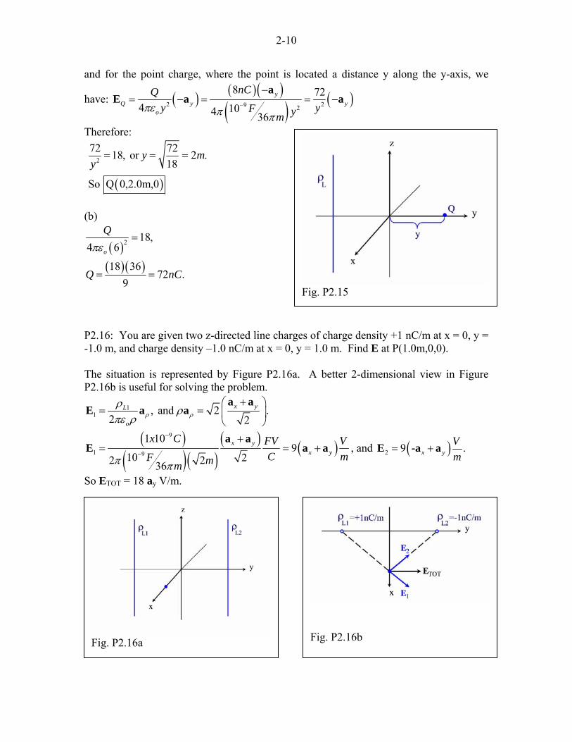
P2.16: You are given two z-directed line charges of charge density +1 nC/m at x = 0, y = -1.0 m, and charge density –1.0 nC/m at x = 0, y = 1.0 m. Find E at P(1.0m,0,0). The situation is represented by Figure P2.16a. A better 2-dimensional view in Figure P2.16b is useful for solving the problem.

11 , and 2 .

2 2x yL

oρ ρ

ρ ρπε ρ

+⎛ ⎞= = ⎜ ⎟

⎝ ⎠

a aE a a

( )( )( )

( ) ( )9

1 9

1 109

10 22 236

x yx y

x C FV VC mF mmπ π

−

−

+= = + a

a aE a ( ), and 2 9 .x y

Vm

= +a aE -

So ETOT = 18 ay V/m.

Fig. P2.16b Fig. P2.16a

2-11

P2.17: MATLAB: Suppose you have a segment of line charge of length 2L centered on the z-axis and having a charge distribution ρL. Compare the electric field intensity at a point on the y-axis a distance d from the origin with the electric field at that point assuming the line charge is of infinite length. The ratio of E for the segment to E for the infinite line is to be plotted versus the ratio L/d using MATLAB. This is similar to MATLAB 2.3. We have for the ideal case

.2 2

L Lideal

o odρ ρρ ρ

πε ρ πε= =E a a

For the actual 2L case, we have an integration to perform (Equation (2.35) with different limits):

( )3 2 2 2 22 2

2 2

4 4

.2

LLL yL

actualo oL L

L yactual

o

ddz zd z dz

Ld L d

ρ ρρ ρπε περ

ρπε

++

− −

⎡ ⎤= = ⎢ ⎥

++ ⎣ ⎦

⎛ ⎞= ⎜ ⎟

+⎝ ⎠

∫aa

E

aE

Now we manipulate these expressions to get the following ratio:

( )2.

1

actual

ideal

LdL

d

=+

EE

In the program, the actual to ideal field ratio is termed “Eratio” and the charged line half-length L ratioed to the distance d is termed “Lod”. % M-File: MLP0217 % % This program is similar to ML0203. % It compares the E-field from a finite length % segment of charge (from -L to +L on the z-axis) % to the E-field from an infinite length line % of charge. The ratio (E from segment to E from % infinite length line) is plotted versus the ratio % Lod=L/d, where d is the distance along the y axis. % % Wentworth, 12/19/02 % % Variables: % Lod the ratio L/d % Eratio ratio of E from segment to E from line clc %clears the command window clear %clears variables % Initialize Lod array and calculate Eratio Lod=0.1:0.01:100;

2-12

Eratio=Lod./(sqrt(1+Lod.^2)); % Plot Eratio versus Lod semilogx(Lod,Eratio) grid on xlabel('Lod=L/d') ylabel('E ratio: segment to line') Executing the program gives Figure P2.17.

Fig. P2.17

So we see that the field from a line segment of charge appears equivalent to the field from an infinite length line if the test point is close to the line. P2.18: A segment of line charge ρL =10 nC/m exists on the y-axis from the origin to y = +3.0 m. Determine E at the point (3.0, 0, 0)m. It is clear from a sketch of the problem in Figure P2.18a that the resultant field will be directed in the x-y plane. The situation is redrawn in a temporary coordinate system in Figure P2.18b.

We have from Eqn (2.34) ( )

32 2 2

.4

zLz z

o

zdz E Ez

ρρ ρ

ρρπε ρ

−= =

+∫

a aE a + a

For Eρ we have:

( )

3

3 2 2 22 2 20

4 4L L

o o

dz zEzz

ρρ ρ ρ ρπε πε ρ ρρ

⎡ ⎤= = ⎢ ⎥

+⎢ ⎥+ ⎣ ⎦∫

With ρ = 3, we then have Eρ = 21.2 V/m. For Ez:

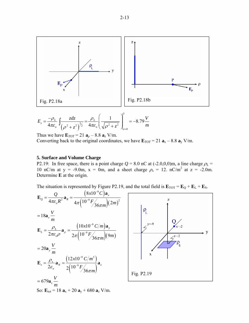
2-13

Fig. P2.18a

Fig. P2.18b

( )

3

3 2 22 2 20

1 8.794 4

L Lz

o oz

zdz VEmzz

ρ ρπε πε ρρ =

⎛ ⎞−⎜ ⎟= = =⎜ ⎟++ ⎝ ⎠

∫ −

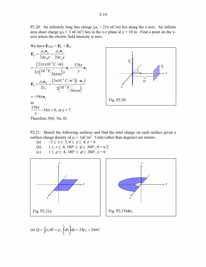
Thus we have ETOT = 21 aρ – 8.8 az V/m. Converting back to the original coordinates, we have ETOT = 21 ax – 8.8 ay V/m. 5. Surface and Volume Charge P2.19: In free space, there is a point charge Q = 8.0 nC at (-2.0,0,0)m, a line charge ρL = 10 nC/m at y = -9.0m, x = 0m, and a sheet charge ρs = 12. nC/m2 at z = -2.0m. Determine E at the origin. The situation is represented by Figure P2.19, and the total field is ETOT = EQ + EL + ES.

( )( )( )

9

2 9 2

8 104 104 236

18

xQ R

o

x

x CQR F mm

Vm

πε π π

−

−= =

=

aE a

a

( )( )( )

9

9

10 102 102 936

20

yLL

o

y

x C m

F mmVm

ρρ

πε ρ π π

−

−= =

=

aE a

a

( )( )

9 2

9

12 102 102 36

679

ss N z

o

z

x C m

Fm

Vm

ρε

π

−

−= =

=

E a

a

a Fig. P2.19

So: Etot = 18 ax + 20 ay + 680 az V/m.

2-14

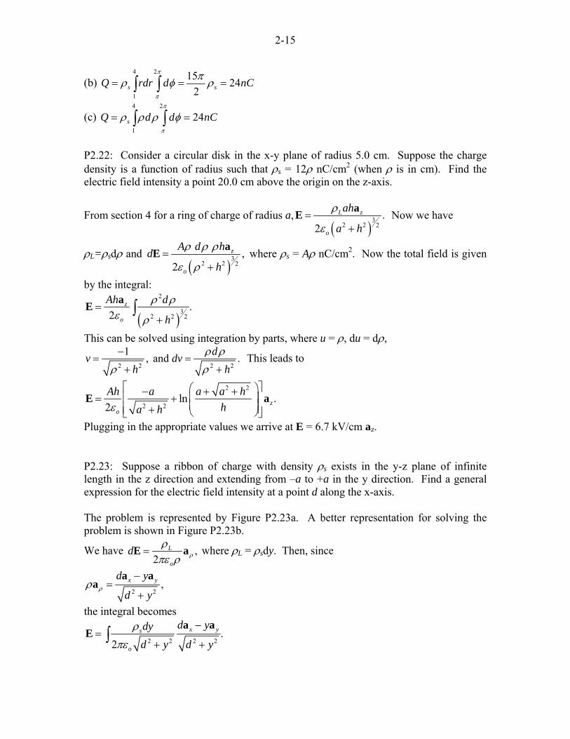
P2.20: An infinitely long line charge (ρL = 21π nC/m) lies along the z-axis. An infinite area sheet charge (ρs = 3 nC/m2) lies in the x-z plane at y = 10 m. Find a point on the y-axis where the electric field intensity is zero. We have ETOT = EL + ES.

( )( )

9

9

2 2

21 10 / 378102 36

L yLL

o o

y y

y

x C myF ym

ρ ρρπε ρ πε

π π

π π

−

−

= =

= =

aaE

a a

Fig. P2.21b&c

Fig. P2.21a

( )( )( )

9 2

9

3 102 102 36

54

ys Ns

o

y

x C m

Fm

ρε

ππ

−

−

−= =

= −

aaE

a

so 378 54 0, or 7.y

yπ π− = =

Therefore, P(0, 7m, 0). P2.21: Sketch the following surfaces and find the total charge on each surface given a surface charge density of ρs = 1nC/m2. Units (other than degrees) are meters.

(a) –3 ≤ x ≤ 3, 0 ≤ y ≤ 4, z = 0 (b) 1 ≤ r ≤ 4, 180° ≤ φ ≤ 360°, θ = π/2 (c) 1 ≤ ρ ≤ 4, 180° ≤ φ ≤ 360°, z = 0

(a) 3 4

3 0

24 24s s sQ dS dx dy nρ ρ ρ−

= = = =∫ ∫ ∫ C

Fig. P2.20

2-15

(b) 4 2

1

15 242s sQ rdr d nC

π

π

πρ φ ρ= = =∫ ∫

(c) 4 2

1

24sQ d dπ

π

ρ ρ ρ φ= =∫ ∫ nC

P2.22: Consider a circular disk in the x-y plane of radius 5.0 cm. Suppose the charge density is a function of radius such that ρs = 12ρ nC/cm2 (when ρ is in cm). Find the electric field intensity a point 20.0 cm above the origin on the z-axis.

From section 4 for a ring of charge of radius a,( )

32 2 2

.2

L z

o

ah

a h

ρ

ε=

+

aE Now we have

ρL=ρsdρ and ( )

32 2 2

,2

z

o

A d hdh

ρ ρ ρ

ε ρ=

+

aE where ρs = Aρ nC/cm2. Now the total field is given

by the integral:

( )2

32 2 2

.2

z

o

Ah d

h

ρ ρε ρ

=+

∫aE

This can be solved using integration by parts, where u = ρ, du = dρ,

2 2 2 2

1 , and .dv dvh h

ρ ρρ ρ

−= =

+ + This leads to

2 2

2 2ln .

2 zo

Ah a a a hha hε

⎡ ⎤⎛ ⎞− + +⎢ ⎥= + ⎜ ⎟⎜ ⎟⎢ ⎥+ ⎝ ⎠⎣ ⎦

E a

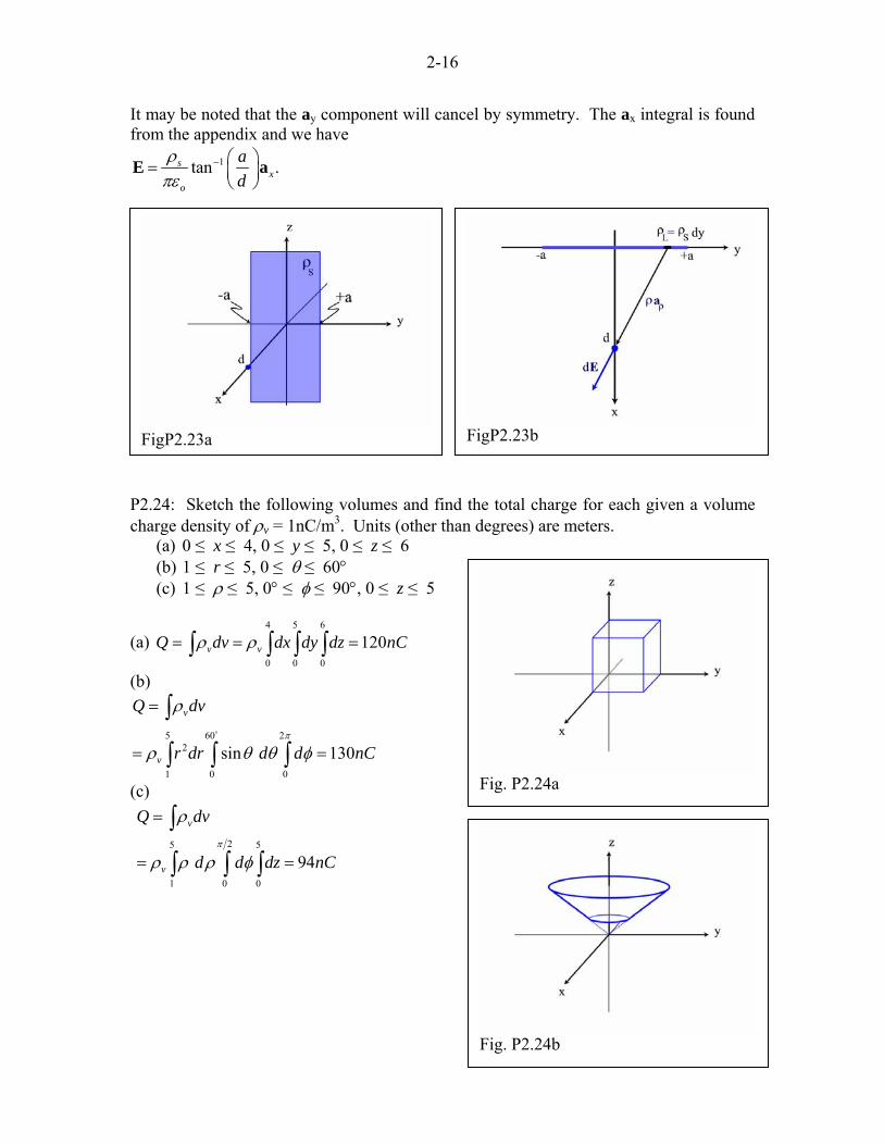
Plugging in the appropriate values we arrive at E = 6.7 kV/cm az. P2.23: Suppose a ribbon of charge with density ρs exists in the y-z plane of infinite length in the z direction and extending from –a to +a in the y direction. Find a general expression for the electric field intensity at a point d along the x-axis. The problem is represented by Figure P2.23a. A better representation for solving the problem is shown in Figure P2.23b.

We have ,2

L

o

d ρρ

πε ρ=E a where ρL = ρsdy. Then, since

2 2,x yd y

d yρρ

−=

+

a aa

the integral becomes

2 2 2 2.

2x ys

o

d ydyd y d y

ρπε

−=

+ +∫

a aE

2-16

It may be noted that the ay component will cancel by symmetry. The ax integral is found from the appendix and we have

1tan .sx

o

ad

ρπε

− ⎛ ⎞= ⎜ ⎟⎝ ⎠

E a

FigP2.23a FigP2.23b

P2.24: Sketch the following volumes and find the total charge for each given a volume charge density of ρv = 1nC/m3. Units (other than degrees) are meters.

(a) 0 ≤ x ≤ 4, 0 ≤ y ≤ 5, 0 ≤ z ≤ 6 (b) 1 ≤ r ≤ 5, 0 ≤ θ ≤ 60°

Fig. P2.24b

(c) 1 ≤ ρ ≤ 5, 0° ≤ φ ≤ 90°, 0 ≤ z ≤ 5

(a) 4 5 6

0 0 0

120v vQ dv dx dy dz nρ ρ= = =∫ ∫ ∫ ∫ C

(b)

5 60 22

1 0 0

sin 130

v

v

Q dv

r dr d d nCπ

ρ

ρ θ θ φ

=

= =

∫

∫ ∫ ∫

Fig. P2.24a (c)

25 5

1 0 0

94

v

v

Q dv

d d dz nCπ

ρ

ρ ρ ρ φ

=

= =

∫

∫ ∫ ∫

2-17

Fig. P2.24c

P2.25: You have a cylinder of 4.00 inch diameter and 5.00 inch length (imagine a can of tomatoes) that has a charge distribution that varies with radius as ρv = (6 ρ) nC/in3 where ρ is in inches. (It may help you with the units to think of this as ρv (nC/in3)= 6 (nC/in4) ρ(in)). Find the total charge contained in this cylinder.

( )2 2 5

2

0 0 0

6 6 160 503vQ dv d d dz d d dz nC nπ

ρ ρ ρ ρ φ ρ ρ φ π= = = = =∫ ∫∫∫ ∫ ∫ ∫ C

P2.26: MATLAB: Consider a rectangular volume with 0.00 ≤ x ≤ 4.00 m, 0.00 ≤ y ≤ 5.00 m and –6.00 m ≤ z ≤ 0.00 with charge density ρv = 40.0 nC/m3. Find the electric field intensity at the point P(0.00,0.00,20.0m). % MLP0226 % calculate E from a rectangular volume of charge % variables % xstart,xstop limits on x for vol charge (m) % ystart,ystop % zstart,zstop % xt,yt,zt test point (m) % rhov vol charge density, nC/m^3 % Nx,Ny,Nz discretization points % dx,dy,dz differential lengths % dQ differential charge, nC % eo free space permittivity (F/m) % dEi differential field vector % dEix,dEiy,dEiz x,y and z components of dEi % dEjx,dEjy,dEjz of dEj % dEkx,dEky,dEkz of dEk % Etot total field vector, V/m

2-18

clc clear % initialize variables xstart=0;xstop=4; ystart=0;ystop=5; zstart=-6;zstop=0; xt=0;yt=0;zt=20; rhov=40e-9; Nx=10;Ny=10;Nz=10; eo=8.854e-12; dx=(xstop-xstart)/Nx; dy=(ystop-ystart)/Ny; dz=(zstop-zstart)/Nz; dQ=rhov*dx*dy*dz; for k=1:Nz for j=1:Ny for i=1:Nx xv=xstart+(i-0.5)*dx; yv=ystart+(j-0.5)*dy; zv=zstart+(k-0.5)*dz; R=[xt-xv yt-yv zt-zv]; magR=magvector(R); uvR=unitvector(R); dEi=(dQ/(4*pi*eo*magR^2))*uvR; dEix(i)=dEi(1); dEiy(i)=dEi(2); dEiz(i)=dEi(3); end dEjx(j)=sum(dEix); dEjy(j)=sum(dEiy); dEjz(j)=sum(dEiz); end dEkx(k)=sum(dEjx); dEky(k)=sum(dEjy); dEkz(k)=sum(dEjz); end Etotx=sum(dEkx); Etoty=sum(dEky); Etotz=sum(dEkz); Etot=[Etotx Etoty Etotz] Now to run the program: Etot =

2-19

-6.9983 -8.7104 79.7668 >> So E = -7.0 ax -8.7 ay + 80. az V/m P2.27: MATLAB: Consider a sphere with charge density ρv = 120 nC/m3 centered at the origin with a radius of 2.00 m. Now, remove the top half of the sphere, leaving a hemisphere below the x-y plane. Find the electric field intensity at the point P(8.00m,0.00,0.00). (Hint: see MATLAB 2.4, and consider that your answer will now have two field components.) % M-File: MLP0227 % % This program modifies ML0204 to find the field % at point P(8m,0,0) from a hemispherical % distribution of charge given by % rhov=120 nC/m^3 from 0 < r < 2m and % pi/2 < theta < pi. % % Wentworth, 12/23/02 % % Variables: % d y axis distance to test point (m) % a sphere radius (m) % dV differential charge volume where % dV=delta_r*delta_theta*delta_phi % eo free space permittivity (F/m) % r,theta,phi spherical coordinate location of % center of a differential charge element % x,y,z cartesian coord location of charge % element % R vector from charge element to P % Rmag magnitude of R % aR unit vector of R % dr,dtheta,dphi differential spherical elements % dEi,dEj,dEk partial field values % Etot total field at P resulting from charge clc %clears the command window clear %clears variables % Initialize variables eo=8.854e-12; d=8;a=2;

2-20

delta_r=40;delta_theta=72;delta_phi=144; % Perform calculation for k=(1:delta_phi) for j=(1:delta_theta) for i=(1:delta_r) r=i*a/delta_r; theta=(pi/2)+j*pi/(2*delta_theta); phi=k*2*pi/delta_phi; x=r*sin(theta)*cos(phi); y=r*sin(theta)*sin(phi); z=r*cos(theta); R=[d-x,-y,-z]; Rmag=magvector(R); aR=R/Rmag; dr=a/delta_r; dtheta=pi/delta_theta; dphi=2*pi/delta_phi; dV=r^2*sin(theta)*dr*dtheta*dphi; dQ=120e-9*dV; dEi=dQ*aR/(4*pi*eo*Rmag^2); dEix(i)=dEi(1); dEiy(i)=dEi(2); dEiz(i)=dEi(3); end dEjx(j)=sum(dEix); dEjy(j)=sum(dEiy); dEjz(j)=sum(dEiz); end dEkx(k)=sum(dEjx); dEky(k)=sum(dEjy); dEkz(k)=sum(dEjz); end Etotx=sum(dEkx); Etoty=sum(dEky); Etotz=sum(dEkz); Etot=[Etotx Etoty Etotz] Now to run the program: Etot = 579.4623 0.0000 56.5317 So E = 580 ax + 57 az V/m. 6. Electric Flux Density

2-21

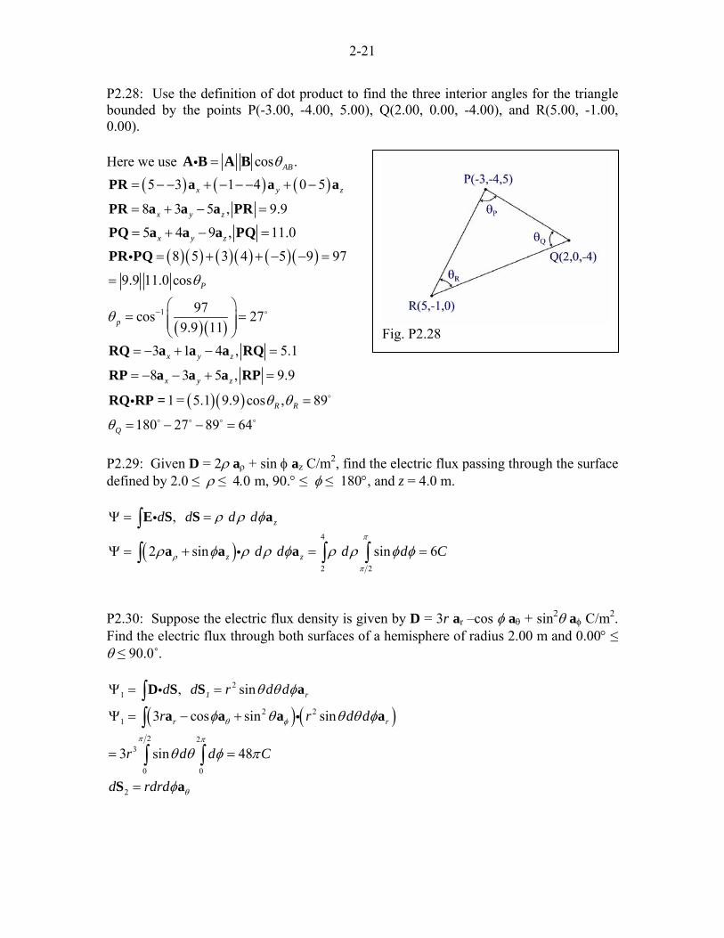
P2.28: Use the definition of dot product to find the three interior angles for the triangle bounded by the points P(-3.00, -4.00, 5.00), Q(2.00, 0.00, -4.00), and R(5.00, -1.00, 0.00). Here we use cos .ABθ=A B A Bi

Fig. P2.28

( ) ( ) ( )5 3 1 4 0 5

8 3 5 , 9.9x y

x y z

= − − + − − − + −

= + − =

PR a a a

PR a a a PRz

5 4 9 , 11.0x y z= + − =PQ a a a PQ

( )( ) ( )( ) ( )( )

( )( )1

8 5 3 4 5 9 97

9.9 11.0 cos

97cos 279.9 11

P

p

θ

θ −

= + + − − =

=

⎛ ⎞= =⎜ ⎟⎜ ⎟

⎝ ⎠

PR PQi

( )( )

3 1 4 , 5.1

8 3 5 , 9.9

1 = 5.1 9.9 cos , 89

180 27 89 64

x y z

x y z

R R

Q

θ θ

θ

= − + − =

= − − + =

=

= − − =

RQ a a a RQ

RP a a a RP

RQ RP =i

P2.29: Given D = 2ρ aρ + sin φ az C/m2, find the electric flux passing through the surface defined by 2.0 ≤ ρ ≤ 4.0 m, 90.° ≤ φ ≤ 180°, and z = 4.0 m.

, zd d d dρ ρ φΨ = =∫E S S ai

( )4

2 2

2 sin sin 6z zd d d d Cπ

ρπ

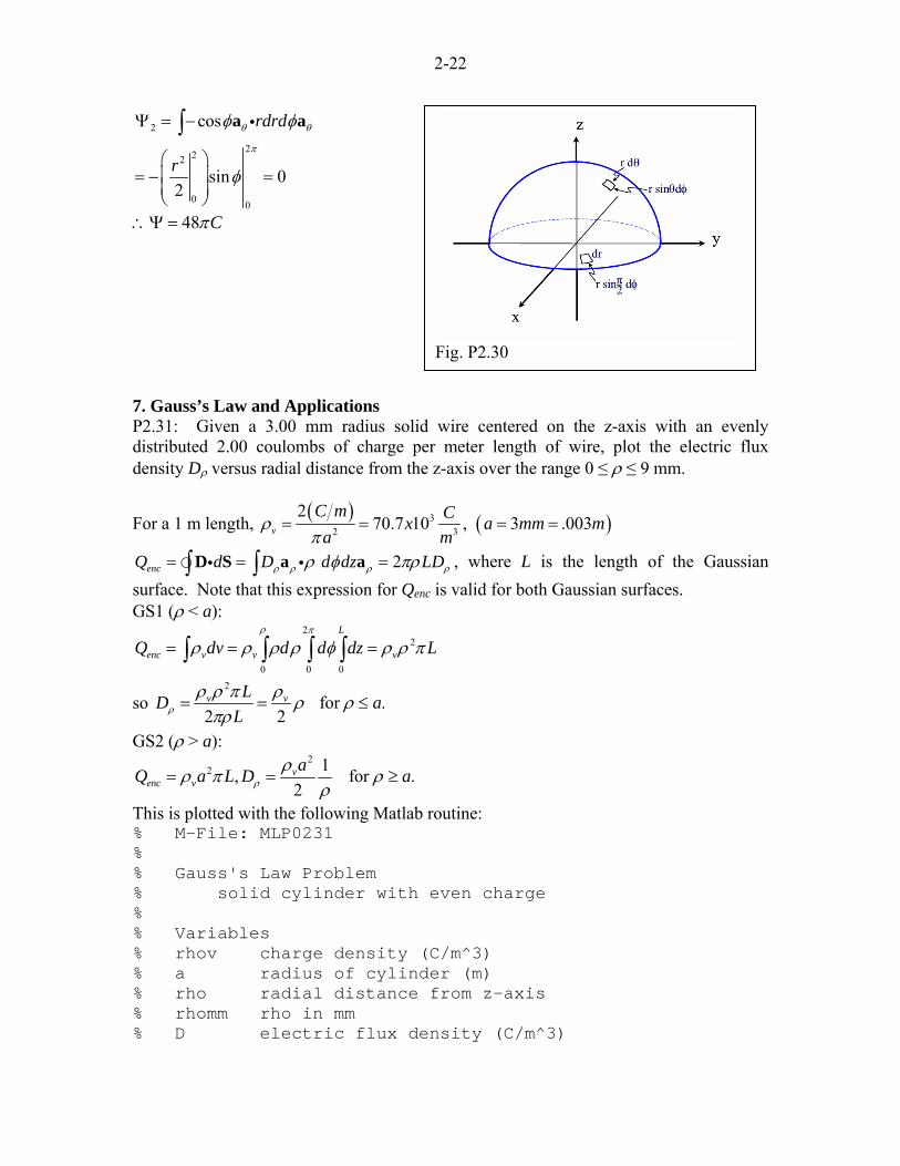
ρ φ ρ ρ φ ρ ρ φ φΨ = + = =∫ ∫a a ai ∫ P2.30: Suppose the electric flux density is given by D = 3r ar –cos φ aθ + sin2θ aφ C/m2. Find the electric flux through both surfaces of a hemisphere of radius 2.00 m and 0.00° ≤ θ ≤ 90.0˚.

21 , sin1 rd d r d dθ θ φΨ = =∫ D S S ai

( ) ( )2 21

2 23

0 0

3 cos sin sin

3 sin 48

r rr r

r d d C

θ φ

π π

φ θ θ θ φ

θ θ φ π

Ψ = − +

= =

∫

∫ ∫

a a a i d d a

2d rdrd θφ=S a

2-22

Fig. P2.30

2

222

0 0

cos

sin 02

rdrd

r

θ θ

π

φ φ

φ

Ψ = −

⎛ ⎞⎜ ⎟= − =⎜ ⎟⎝ ⎠

∫ a ai

48 Cπ∴Ψ = 7. Gauss’s Law and Applications P2.31: Given a 3.00 mm radius solid wire centered on the z-axis with an evenly distributed 2.00 coulombs of charge per meter length of wire, plot the electric flux density Dρ versus radial distance from the z-axis over the range 0 ≤ ρ ≤ 9 mm.

For a 1 m length, ( ) ( )32 3

270.7 10 , 3 .003v

C m Cx a mm ma m

ρπ

= = = =

2encQ d D d dz LDρ ρ ρρ φ πρ= = =∫ ∫D S a ai i ρ

L

, where L is the length of the Gaussian surface. Note that this expression for Qenc is valid for both Gaussian surfaces. GS1 (ρ < a):

22

0 0 0

L

enc v v vQ dv d d dzρ π

ρ ρ ρ ρ φ ρ ρ π= = =∫ ∫ ∫ ∫

so 2

for .2 2v vLD a

Lρρ ρ π ρ ρ ρ

πρ= = ≤

GS2 (ρ > a): 2

2 1, for 2v

enc vaQ a L Dρ

ρρ π ρρ

= = .a≥

This is plotted with the following Matlab routine: % M-File: MLP0231 % % Gauss's Law Problem % solid cylinder with even charge % % Variables % rhov charge density (C/m^3) % a radius of cylinder (m) % rho radial distance from z-axis % rhomm rho in mm % D electric flux density (C/m^3)

2-23

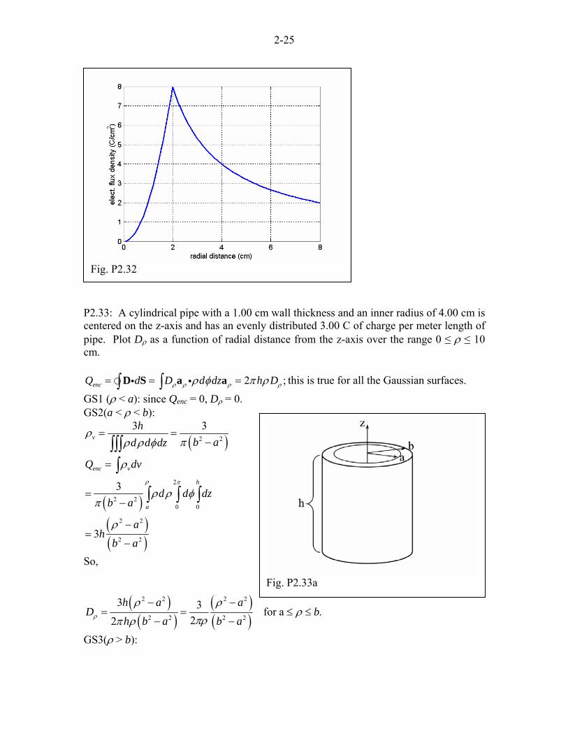
% N number of data points % maxrad max radius for plot (m) clc;clear; % initialize variables rhov=70.7e3; a=0.003; maxrad=.009; N=100; bndy=round(N*a/maxrad); for i=1:bndy rho(i)=i*maxrad/N; rhomm(i)=rho(i)*1000; D(i)=rhov*rho(i)/2; end for i=bndy+1:N rho(i)=i*maxrad/N; rhomm(i)=rho(i)*1000; D(i)=(rhov*a^2)/(2*rho(i)); end plot(rhomm,D) xlabel('radial distance (mm)') ylabel('elect. flux density (C/m^2)') grid on P2.32: Given a 2.00 cm radius solid wire centered on the z-axis with a charge density ρv = 6ρ C/cm3 (when ρ is in cm), plot the electric flux density Dρ versus radial distance from the z-axis over the range 0 ≤ ρ ≤ 8 cm.

Fig. P2.31

2-24

Choose Gaussian surface length L, and as usual we have

2encQ d D d dz L ,Dρ ρ ρρ φ π ρ= ∫ ∫D S = a ai i ρ=

,

valid for both Gaussian surfaces.

In GS1 (ρ < a): 2 36 4enc vQ dv d d dz Lρ ρ ρ φ π ρ= = =∫ ∫

so 3

24 2 for .2

LD aLρ

π ρ ρ ρπ ρ

= = ≤

For GS2 (ρ > a): 3

3 24 , for .encaQ La Dρπ ρρ

= = a≥

This is plotted for the problem values in the following Matlab routine. % M-File: MLP0232 % % Gauss's Law Problem % solid cylinder with radially-dependent charge % % Variables % a radius of cylinder (cm) % rho radial distance from z-axis % D electric flux density (C/cm^3) % N number of data points % maxrad max radius for plot (cm) clc;clear; % initialize variables a=2; maxrad=8; N=100; bndy=round(N*a/maxrad); for i=1:bndy rho(i)=i*maxrad/N; D(i)=2*rho(i)^2; end for i=bndy+1:N rho(i)=i*maxrad/N; D(i)=(2*a^3)/rho(i); end plot(rho,D) xlabel('radial distance (cm)') ylabel('elect. flux density (C/cm^2)') grid on

2-25

Fig. P2.32

P2.33: A cylindrical pipe with a 1.00 cm wall thickness and an inner radius of 4.00 cm is centered on the z-axis and has an evenly distributed 3.00 C of charge per meter length of pipe. Plot Dρ as a function of radial distance from the z-axis over the range 0 ≤ ρ ≤ 10 cm.

2 ;encQ d D d dz h Dρ ρ ρρ φ π ρ= = =∫ ∫D S a ai i ρ this is true for all the Gaussian surfaces.

GS1 (ρ < a): since Qenc = 0, Dρ = 0. GS2(a < ρ < b):

( )2 2

3 3v

hb ad d dz

ρπρ ρ φ

= =−∫∫∫

( )( )( )

2

2 20 0

2 2

2 2

3

3

enc v

h

a

Q dv

d d db a

ah

b a

ρ π

ρ

ρ ρ φπ

ρ

=

=−

−=

−

∫

∫ ∫ ∫ z

So,

( )( )

( )( )

2 2 2 2

2 2 2 2

3 3 for a .22

h a aD b

h b a b aρ

ρ ρρ

πρπ ρ

− −= =

− −≤ ≤

Fig. P2.33a

GS3(ρ > b):

2-26

Qenc = 3h, 3 for .2

D bρ ρπρ

= >

A plot with the appropriate values is generated by the following Matlab routine: % M-File: MLP0233 % Gauss's Law Problem % cylindrical pipe with even charge distribution % % Variables % a inner radius of pipe (m) % b outer radius of pipe (m) % rho radial distance from z-axis (m) % rhocm radial distance in cm % D electric flux density (C/cm^3) % N number of data points % maxrad max radius for plot (m) clc;clear; % initialize variables a=.04;b=.05;maxrad=0.10;N=100; bndya=round(N*a/maxrad); bndyb=round(N*b/maxrad); for i=1:bndya rho(i)=i*maxrad/N; rhocm(i)=rho(i)*100; D(i)=0; end for i=bndya+1:bndyb rho(i)=i*maxrad/N; rhocm(i)=rho(i)*100; D(i)=(3/(2*pi*rho(i)))*((rho(i)^2-a^2)/(b^2-a^2)); end for i=bndyb+1:N rho(i)=i*maxrad/N; rhocm(i)=rho(i)*100; D(i)=3/(2*pi*rho(i)); end plot(rhocm,D) xlabel('radial distance (cm)') ylabel('elect. flux density (C/m^2)') grid on

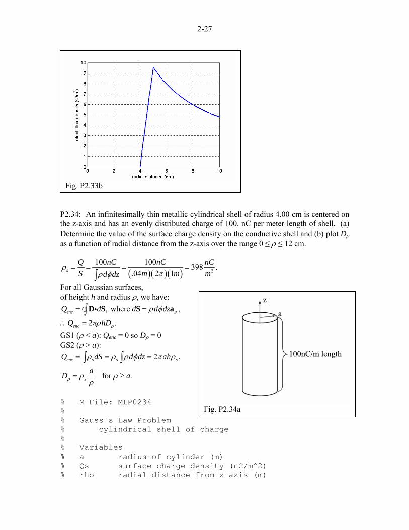
2-27

PtDa

Fo

∴

GG

%%%%%%%%%

Fig. P2.33b

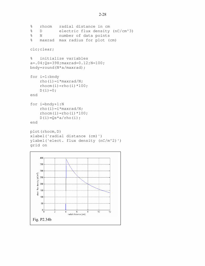
2.34: An infinitesimally thin metallic cylindrical shell of radius 4.00 cm is centered on he z-axis and has an evenly distributed charge of 100. nC per meter length of shell. (a) etermine the value of the surface charge density on the conductive shell and (b) plot Dρ

s a function of radial distance from the z-axis over the range 0 ≤ ρ ≤ 12 cm.

( )( )( ) 2

100 100 398 ..04 2 1s

Q nC nC nS m md dz

ρπρ φ

= = = =∫

Cm

z

or all Gaussian surfaces, f height h and radius ρ, we have:

, where ,

2 .enc

enc

Q d d d d

Q hDρ

ρ

ρ φ

πρ

= =

=∫ D S S ai

S1 (ρ < a): Qenc = 0 so Dρ = 0 S2 (ρ > a):

2 ,

for .

enc s s s

s

Q dS d dz ah

aD aρ

ρ ρ ρ φ π ρ

ρ ρρ

= = =

= ≥

∫ ∫

Fig. P2.34a M-File: MLP0234 Gauss's Law Problem cylindrical shell of charge Variables a radius of cylinder (m) Qs surface charge density (nC/m^2) rho radial distance from z-axis (m)

2-28

% rhocm radial distance in cm % D electric flux density (nC/cm^3) % N number of data points % maxrad max radius for plot (cm) clc;clear; % initialize variables a=.04;Qs=398;maxrad=0.12;N=100; bndy=round(N*a/maxrad); for i=1:bndy rho(i)=i*maxrad/N; rhocm(i)=rho(i)*100; D(i)=0; end for i=bndy+1:N rho(i)=i*maxrad/N; rhocm(i)=rho(i)*100; D(i)=Qs*a/rho(i); end plot(rhocm,D) xlabel('radial distance (cm)') ylabel('elect. flux density (nC/m^2)') grid on

Fig. P2.34b

2-29

P2.35: A spherical charge density is given by ρv = ρo r/a for 0 ≤ r ≤ a, and ρv = 0 for r > a. Derive equations for the electric flux density for all r.

2 sin 4 .enc r r r rQ d D r d d rθ θ φ π= = =∫ ∫D S a ai i 2D This is valid for each Gaussian surface.

GS1 (r < a): 2 4

3

0 0 0

sin .r

o oenc v

rQ dv r dr d da a

π πρ πρ θ θ φ= = =∫ ∫ ∫ ∫ρ

So 4

22 for .

4 4o o

rrD r

a r aπρ ρ

π= = ≤r a

GS2 (r > a): 3

32, for .

4o

enc o raQ a D rr

ρπρ= = a≥

2D

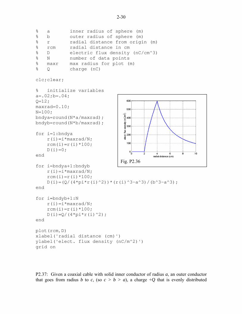
P2.36: A thick-walled spherical shell, with inner radius 2.00 cm and outer radius 4.00 cm, has an evenly distributed 12.0 nC charge. Plot Dr as a function of radial distance from the origin over the range 0 ≤ r ≤ 10 cm. Here we’ll let a = inner radius and b = outer radius. Then

2 sin 4 ;enc r r r rQ d D r d d rθ θ φ π= = =∫ ∫D S a ai i This is true for each Gaussian surface. The volume containing charge is

( )2

2 3

0 0

4sin .3

b

a

v r dr d d b aπ π

θ θ φ π= =∫ ∫ ∫ 3−

So ( )3 3

3 .4v

Q Qv b a

ρπ

= =−

Now we can evaluate Qenc for each Gaussian surface. GS1 (r < a): Qenc = 0 so Dr = 0.

GS2 (a < r < b): ( )2

2 3

0 0

4sin .3

rv

enc v va

Q dv r dr d d r aπ π ρ πρ ρ θ θ φ= = = −∫ ∫ ∫ ∫ 3

Inserting our value for ρv, we find ( )( )

3 3

2 3 3 for .

4r

r aQD ar b aπ

−= ≤

−r b≤

GS3 (r >b): Qenc = Q, 2 , for .4r

QD rr

bπ

= ≥

This is plotted for appropriate values using the following Matlab routine: % M-File: MLP0236 % Gauss's Law Problem % thick spherical shell with even charge % % Variables

2-30

% a inner radius of sphere (m) % b outer radius of sphere (m) % r radial distance from origin (m) % rcm radial distance in cm % D electric flux density (nC/cm^3) % N number of data points % maxr max radius for plot (m) % Q charge (nC) clc;clear; % initialize variables a=.02;b=.04;

Fig. P2.36

Q=12; maxrad=0.10; N=100; bndya=round(N*a/maxrad); bndyb=round(N*b/maxrad); for i=1:bndya r(i)=i*maxrad/N; rcm(i)=r(i)*100; D(i)=0; end for i=bndya+1:bndyb r(i)=i*maxrad/N; rcm(i)=r(i)*100; D(i)=(Q/(4*pi*r(i)^2))*(r(i)^3-a^3)/(b^3-a^3); end for i=bndyb+1:N r(i)=i*maxrad/N; rcm(i)=r(i)*100; D(i)=Q/(4*pi*r(i)^2); end plot(rcm,D) xlabel('radial distance (cm)') ylabel('elect. flux density (nC/m^2)') grid on P2.37: Given a coaxial cable with solid inner conductor of radius a, an outer conductor that goes from radius b to c, (so c > b > a), a charge +Q that is evenly distributed

2-31

throughout a meter length of the inner conductor and a charge –Q that is evenly distributed throughout a meter length of the outer conductor, derive equations for the electric flux density for all ρ. You may orient the cable in any way you wish. We conveniently center the cable on the z-axis. Then, for a Gaussian surface of length L,

2encQ d L ;Dρπρ= =∫ D Si valid for all Gaussian surfaces.

GS1: (ρ < a): ( )( )2

;1v

Qm a

ρπ

=

22

1 20 0 0

2

2 2

;

for 2 2

L

v vQLQ dv d d dza

QL QD aa L a

ρ π

ρ

ρ ρ ρ ρ φ ρ

ρ ρ ρπρ π

= = =

= = ≤

∫ ∫ ∫ ∫

GS2 (a < ρ < b): 2 ; for .2 2QL QQ QL D a b

Lρ ρπρ πρ

= = = ≤ ≤

GS3 (b < ρ < c): ( ) ( )3 2 2

, where 1vo vo

QQ Q dvm c b

ρ ρπ

−= + =

−∫

( )( )( )

2 22

3 2 2 2 20 0

L

b

cQQ Q d d dz Qc b c b

ρ π ρρ ρ φ

π

−−= + =

− −∫ ∫ ∫

so ( )( )

2 2

2 2 for .

2cQD bc bρ

ρρ

πρ−

= ≤−

c≤

GS4 (ρ > c): Qenc = 0, Dρ = 0. 8. Divergence and the Point Form of Gauss’s Law P2.38: Determine the charge density at the point P(3.0m,4.0m,0.0) if the electric flux density is given as D = xyz az C/m2.

( ) .zv

xyzD xyz z

ρ∂∂

∇ = = = =∂ ∂

Di

ρv(3,4,0)=(3)(4)=12 C/m3. P2.39: Given D = 3ax +2xyay +8x2y3az C/m2, (a) determine the charge density at the point P(1,1,1). Find the total flux through the surface of a cube with 0.0 ≤ x ≤ 2.0m, 0.0 ≤ y ≤ 2.0m and 0.0 ≤ z ≤ 2.0m by evaluating (b) the left side of the divergence theorem and (c) the right side of the divergence theorem.

2-32

(a) ( ) ( ) 3= 2 2 , 1,1,1 2vCxy x

y mρ∂

∇ = =∂

Di .

∫

(b) d dv= ∇ = + + + + +∫ ∫ ∫ ∫ ∫ ∫ ∫top bottom left right front back

D S Di i

2 22 3 2 3

0 0

8 8z ztop

85.3x y dxdy x dx y dy C= =∫ ∫ ∫ ∫a ai =

( )2 38 85.3z zbottom

x y dxdy= − = −∫ ∫ a ai C

( )2 0y yleft

x y dxdz= −∫ ∫ y=0a ai =

y=22 1y y

right

6x y dxdz= =∫ ∫ a ai C

2

2

C

3 1x xfront

dydz C= =∫ ∫ a ai

( )3 1x xback

dydz C= − = −∫ ∫ a ai

16 .encQ d∴ = =∫ D Si

(c) ( )2 2 2

0 0 0

2 2 ; 2 16 .xy x dv xdx dy dz Cy

∂∇ = ∇ =

∂ ∫ ∫ ∫ ∫D = Di i =

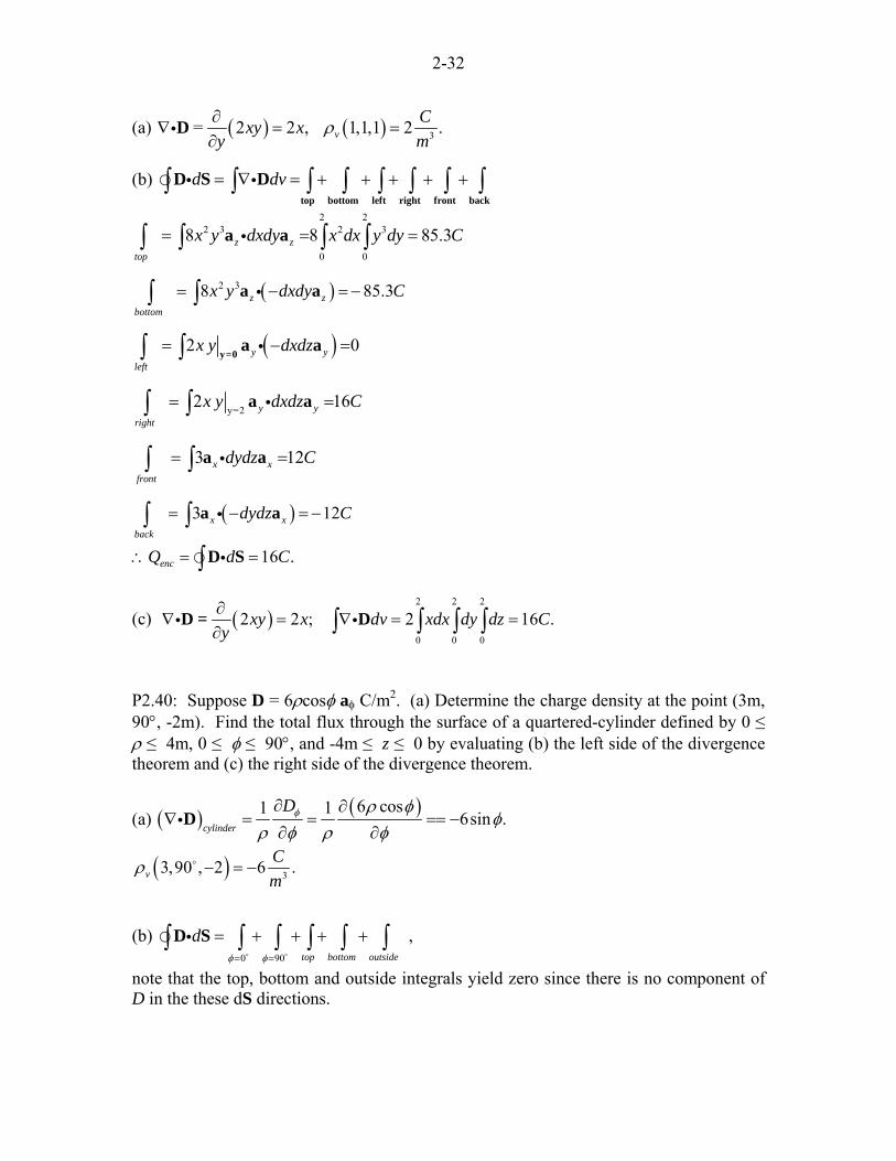
P2.40: Suppose D = 6ρcosφ aφ C/m2. (a) Determine the charge density at the point (3m, 90°, -2m). Find the total flux through the surface of a quartered-cylinder defined by 0 ≤ ρ ≤ 4m, 0 ≤ φ ≤ 90°, and -4m ≤ z ≤ 0 by evaluating (b) the left side of the divergence theorem and (c) the right side of the divergence theorem.

(a) ( ) ( )6 cos1 1 6sin .cylinder

Dφ ρ φφ

ρ φ ρ φ∂ ∂

∇ = = == −∂ ∂

Di

( ) 33,90 , 2 6 .vCm

ρ − = −

(b) 0 90

,top bottom outside

dφ φ= =

= + + + +∫ ∫ ∫ ∫ ∫ ∫D Si

note that the top, bottom and outside integrals yield zero since there is no component of D in the these dS directions.

2-33

( )0

0

6 cos 192d dz Cφ φφφ

ρ φ ρ=

=

= − =∫ ∫ a ai −

( )90

90

6 cos 0d dzφ φφφ

ρ φ ρ=

=

= =∫ ∫ a ai

So, 192 .d C= −∫ D Si (c)

90 4 0

0 0 4

6sin ,

6 sin 192 .

dv d d dz

dv d d dz C

φ ρ ρ φ

φ φ ρ ρ−

∇ = − =

∇ = − = −∫ ∫ ∫ ∫

D

D

i

i

P2.41: Suppose D = r2sinθ ar + sinθcosφ aφ C/m2. (a) Determine the charge density at the point (1.0m, 45°, 90°). Find the total flux through the surface of a volume defined by 0.0 ≤ r ≤ 2.0 m, 0.0° ≤ θ ≤ 90.°, and 0.0 ≤ φ ≤ 180° by evaluating (b) the left side of the divergence theorem and (c) the right side of the divergence theorem. The volume is that of a quartered-sphere, as indicated in Figure P2.41. (a)

( )

( )

22

3

1 1 sin= = 4 sinsin

1,45 ,90 1.83

r v

v

Dr D r

r r r rCm

φ φ = , θ ρθ φ

ρ

∂∂∇ + −

∂ ∂

=

Di

(b) 20 180 90 90

; note that 0 since 0.r

d Dθφ φ θ θ== = = =

= + + + = =∫ ∫ ∫ ∫ ∫ ∫D Si

( )00

sin cos 2rdrd Cφ φφφ

θ φ θ=

=

= −∫ ∫ a ai = −

180180

sin cos 2rdrd Cφ φφφ

θ φ θ=

=

= =∫ ∫ a ai −

( )2 90

2 2 4 2

2 0 0 0

sin sin sin 8 1 cos 2 4r rr

r r d d r d d dπ π

2Cθ θ θ φ θ θ φ π θ θ π=

= = = −∫ ∫ ∫ ∫ ∫a ai =

Summing these terms we have Q = 4(π2 – 1)C = 35.5C. (c)

2-34

2

2 22 23 2 2

0 0 0 0 0 0

sin4 sin sin

4 sin sin sin 4 4 35.5 .

dv r r drd dr

r dr d d rdr d d Cπ ππ π

φθ θ θ φ

θ θ φ θ θ φ φ π

⎛ ⎞∇ = −⎜ ⎟⎝ ⎠

= − = −

∫ ∫

∫ ∫ ∫ ∫ ∫ ∫

Di

=

Fig. P2.41

9. Electric Potential P2.42: A sheet of charge density ρs = 100 nC/m2 occupies the x-z plane at y = 0. (a) Find the work required to move a 2.0 nC charge from P(-5.0m, 10.m, 2.0m) to M(2.0m, 3.0m, 0.0). (b)Find VMP.

(a) ; so we need for the sheet charge.M

P

W Q d= − ∫ E L Ei

( )( )

93

12

100 105.65 10

2 2 8.854 10s

N yo

x C FV VxC mx F m

ρε

−

−= = =E a a ya

Notice that we are only concerned with movement in the y-direction. We then have: 3

9 3

10

2 10 5.65 10 79y

y yy

V JW x C x dym CV

Jµ=

−

=

⎛ ⎞ ⎛ ⎞= − =⎜ ⎟ ⎜ ⎟⎝ ⎠ ⎝ ⎠∫ a ai

(b) ( )( )9

7939.5 ; so 40 .

2 10MP MP

JW CVV k V V kVQ Jx C

µ−

= = = =

P2.43: A surface is defined by the function 2x + 4y2 –ln z = 12. Use the gradient equation to find a unit vector normal to the plane at the point (3.00m,2.00m,1.00m).

2-35

Let then 22 4 ln 12F x y z= + − = ,1; 2 8 ,x x

F F yF z

∇= ∇ = + −

∇a a a y za

At (3,2,1),

2 2 22 16 , 2 16 1 16.16,

0.124 0.990 0.062x y z

N x y z

F F∇ = + − ∇ = + + =

= + −

a a a

a a a a

P2.44: For the following potential distributions, use the gradient equation to find E.

(a) V = x+y2z (V) (b) V = ρ2sinφ(V) (c) V = r sinθ cosφ (V).

(a) 22x yV yz= −∇ = − − −E a a zy a

(b) 1 2 sin coszV V VV

zρ φ ρ φρ φ ρ φρ ρ φ

⎛ ⎞∂ ∂ ∂= −∇ = − + + = − −⎜ ⎟∂ ∂ ∂⎝ ⎠

E a a a a a

(c) 1 1 sin cos cos cos sin

sinV V VVr r rρ θ φ ρ θ φθ φ θ φ

θ θ φ⎛ ⎞∂ ∂ ∂

= −∇ = − + + = − − +⎜ ⎟∂ ∂ ∂⎝ ⎠E a a a a a φa

P2.45: A 100 nC point charge is located at the origin. (a) Determine the potential difference VBA between the point A(0.0,0.0,-6.0)m and point B(0.0,2.0,0.0)m. (b) How much work would be done to move a 1.0 nC charge from point A to point B against the electric field generated by the 100 nC point charge?

(a) .A

BAA

V d= −∫E Li

The potential difference is only a function of radial distance from the origin. Letting ra = 6m and rb = 2m, we then have

2

1 1 300 .4 4

b

a

r

BA r ro o b ar

Q QV drr r rπε πε

⎛ ⎞= − = − =⎜ ⎟

⎝ ⎠∫ a ai V

(b) ( )( )92 10 300 300BA

JW Q V C V nJCV

−= = =

P2.46: MATLAB: Suppose you have a pair of charges Q1(0.0, -5.0m, 0.0) = 1.0 nC and Q2(0.0, 5.0m, 0.0) = 2.0 nC. Write a MATLAB routine to calculate the potential VRO moving from the origin to the point R(5.0m, 0.0, 0.0). Your numerical integration will involve choosing a step size ∆L and finding the field at the center of the step. You should try several different step sizes to see how much this affects the solution.

2-36

% M-File: MLP0246 % % Modify ML0207 to calculate the potential % difference going from the origin (O) to the point % R(5,0,0) given a pair of point charges % Q1(0,-5,0)=1nC and Q2(0,5,0)=2nC. % % The approach will be to break up the distance % from O to R into k sections. The total field E will % be found at the center of each section (located % at point P) and then dot(Ep,dLv) will give the % potential drop across the kth section. Total % potential is found by summing the potential drops. % % Wentworth, 1/7/03 % % Variables: % Q1,Q2 the point charges, in nC % k number of numerical integration steps % dL magnitude of one step % dLv vector for a step % x(n) x location at center of section at P % R1,R2 vector from Q1,Q2 to P % E1,E2 electric fields from Q1 & Q2 at P % Etot total electric field at P % V(n) portion of dot(Etot,dL) at P clc %clears the command window clear %clears variables % Initialize variables k=64; Q1=1; Q2=2; dL=5/k; dLv=dL*[1 0 0]; % Perform calculation for n=1:k x(n)=(n-1)*dL+dL/2; R1=[x(n) 5 0]; R2=[x(n) -5 0]; Rmag1=magvector(R1); Rmag2=magvector(R2); E1=9*Q1*R1/Rmag1^3;

2-37

E2=9*Q2*R2/Rmag2^3; Etot=E1+E2; V(n)=dot(Etot,dLv); end Vtot=sum(-V) Now running the program: Vtot = -1.5817 So VRO = -1.6 V. P2.47: For an infinite length line of charge density ρL = 20 nC/m on the z-axis, find the potential difference VBA between point B(0, 2m, 0) and point A(0, 1m, 0).

( )

; , ,2

so ln 2 2502 2

BL

BAoA

BL L

BAo oA

V d d d

V d

ρ ρ

ρ ρ

ρ ρπε ρ

ρ ρρπε ρ πε

= − = =

−= − = = −

∫

∫

E L E a L a

a a

i

i V

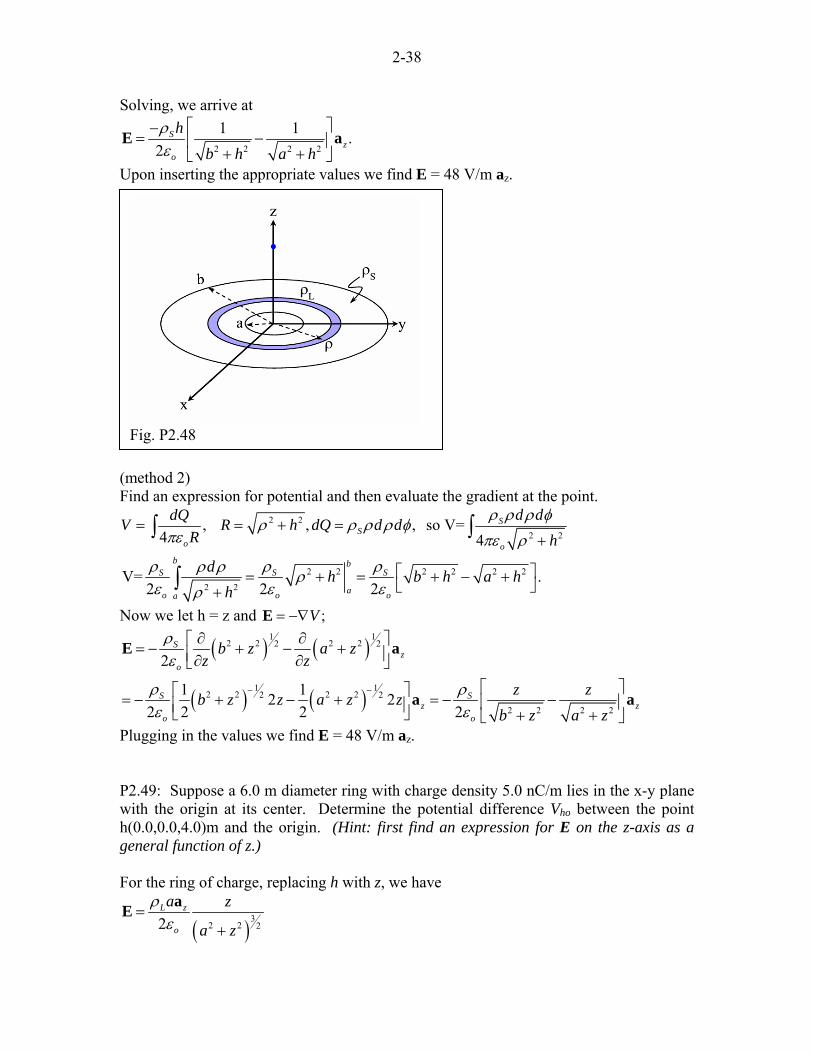
P2.48: Find the electric field at point P(0.0,0.0,8.0m) resulting from a surface charge density ρs = 5.0 nC/m2 existing on the z = 0 plane from ρ = 2.0 m to ρ = 6.0 m. Assume V = 0 at a point an infinite distance from the origin. (Method 1) For a ring of charge it was previously found that

( )3

2 2 2.

2L z

o

ah

a h

ρ

ε=

+

aE

We can then break up our disk into differential rings (see Figure P2.48), each contributing dE as:

( )3

2 2 2, where we've used .

2S

z Lo

h dd dh

Sρ ρ ρ ρ ρ ρ

ε ρ= =

+E a

So we then have

( )3

2 2 2.

2S z

o

h d

h

ρ ρ ρε ρ

=+

∫aE

This is easy to integrate if we let u = ρ2 + h2, then du = 2 ρ dρ, and we have

32

2 2

2 14 4 2

b

S z S z S z

o o o a

h h hu duu h

ρ ρ ρε ε ε ρ

− −−= = =

+∫

a a aE

2-38

Solving, we arrive at

2 2 2 2

1 1 .2

Sz

o

hb h a h

ρε

⎡ ⎤−= −⎢ ⎥

+ +⎣ ⎦E a

Upon inserting the appropriate values we find E = 48 V/m az.

Fig. P2.48

(method 2) Find an expression for potential and then evaluate the gradient at the point.

2 2

2 2, , , so V=

4 4S

So o

d ddQV R h dQ d dR h

ρ ρ ρ φρ ρ ρ ρ φπε πε ρ

= = + =+

∫ ∫

2 2 2 2 2 2

2 2V= .

2 2 2

b bS S S

ao o oa

d h b h ah

ρ ρ ρρ ρ ρε ε ερ

h⎡ ⎤= + = + − +⎣ ⎦+∫

Now we let h = z and ;V= −∇E

( ) ( )

( ) ( )

1 12 2 2 22 2

1 12 2 2 22 2

2 2 2 2

2

1 12 22 2 2 2

Sz

o

S Sz z

o o

b z a zz z

z zb z z a z zb z a z

ρε

ρ ρε ε

− −

∂ ∂⎡ ⎤= − + − +⎢ ⎥∂ ∂⎣ ⎦

⎡ ⎤⎡ ⎤= − + − + = − −⎢ ⎥⎢ ⎥⎣ ⎦ + +⎣ ⎦

E a

a a

Plugging in the values we find E = 48 V/m az. P2.49: Suppose a 6.0 m diameter ring with charge density 5.0 nC/m lies in the x-y plane with the origin at its center. Determine the potential difference Vho between the point h(0.0,0.0,4.0)m and the origin. (Hint: first find an expression for E on the z-axis as a general function of z.) For the ring of charge, replacing h with z, we have

( )3

2 2 22L z

o

a z

a z

ρε

=+

aE

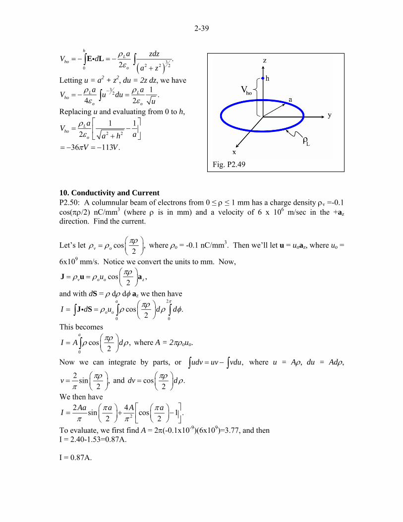
2-39

( )3

2 2 20

.2

hL

hoo

a zdzV da z

ρε

= − = −+

∫ ∫E Li

Fig. P2.49

Letting u = a2 + z2, du = 2z dz, we have 3

2 1 .4 2

L Lho

o o

a aV u duu

ρ ρε ε

−= − =∫

Replacing u and evaluating from 0 to h,

2 2

1 12

36 113 .

Lho

o

aVaa h

V V

ρε

π

⎡ ⎤= −⎢ ⎥

+⎣ ⎦= − = −

10. Conductivity and Current P2.50: A columnular beam of electrons from 0 ≤ ρ ≤ 1 mm has a charge density ρv =-0.1 cos(πρ/2) nC/mm3 (where ρ is in mm) and a velocity of 6 x 106 m/sec in the +az direction. Find the current.

Let’s let cos ,2v o

πρρ ρ ⎛ ⎞= ⎜ ⎟⎝ ⎠

where ρo = -0.1 nC/mm3. Then we’ll let u = uoaz, where uo =

6x109 mm/s. Notice we convert the units to mm. Now,

cos ,2v o ou πρρ ρ ⎛ ⎞= = ⎜ ⎟

⎝ ⎠J u az

and with dS = ρ dρ dφ az we then have 2

0 0

cos .2

a

o oI d u d dππρρ ρ ρ⎛ ⎞= = ⎜ ⎟

⎝ ⎠∫ ∫J Si φ∫

This becomes

0

cos ,2

a

I A πρ dρ ρ⎛ ⎞= ⎜ ⎟⎝ ⎠∫ where A = 2πρouo.

Now we can integrate by parts, or ,udv uv vdu= −∫ ∫ where u = Aρ, du = Adρ,

2 sin ,2

v πρπ

⎛ ⎞= ⎜ ⎟⎝ ⎠

and cos .2

dv dπρ ρ⎛ ⎞= ⎜ ⎟⎝ ⎠

We then have

2

2 4sin cos 1 . 2 2

Aa a A aI π ππ π

⎡ ⎤⎛ ⎞ ⎛ ⎞= + −⎜ ⎟ ⎜ ⎟⎢ ⎥⎝ ⎠ ⎝ ⎠⎣ ⎦To evaluate, we first find A = 2π(-0.1x10-9)(6x109)=3.77, and then I = 2.40-1.53=0.87A. I = 0.87A.

2-40

P2.51: Two spherical conductive shells of radius a and b (b > a) are separated by a material with conductivity σ. Find an expression for the resistance between the two spheres. First find E for a < r < b, assuming +Q at r = a and –Q at r = b. From Gauss’s law:

24 ro

Qrπε

=E a

Now find Vab:

2

2

4

1 1 .4 4 4

a a

ab r rob b

aa

bo o ob

QV d drr

Q dr Q Qr r a

πε

πε πε πε

= − = −

− ⎛ ⎞= = = −⎜ ⎟⎝ ⎠

∫ ∫

∫

E L a ai i

1b

Now can find I: 2

2

2

0 0

1 sin

sin .

r ro

o o

QI d = d = r d d4 r

Q Qd d4

π π

σ σ θπε

σ σθ θ φπε ε

=

= =

∫ ∫ ∫

∫ ∫

J S E S a ai i i θ φ

Finally, 1 1 14

abVRI a bπσ

⎛ ⎞= = −⎜ ⎟⎝ ⎠

P2.52: The typical length of each piece of jumper wire on a student’s protoboard is 5.0 cm. Assuming AWG-20 (wire diameter 0.812 mm) copper wire, (a) determine the resistance for this length of wire. (b) Determine the power dissipated in the wire for 10. mA of current.

(a)( ) ( )22 7 3

1 1 0.05 1.675.8 10 0.406 10

L mR ma x S m x mσ π π −

= = = Ω

so R = 1.7 mΩ (b) ( ) ( )22 3 310 10 1.7 10 170P I R x A x nW− −= = Ω =

P2.53: A densely wrapped coil of AWG-22 (0.644 mm diameter) copper magnet wire is 150 m long. The wire has a very thin insulative sheath. Determine the resistance for this length of wire.

( )22 7 3

1 1 150 7.945.8 10 0.322 10

L mRa x S m x mσ π π −

= = = Ω

so R = 7.9Ω

2-41

P2.54: Determine an expression for the power dissipated per unit length in coaxial cable of inner radius a, outer radius b, and conductivity between the conductors σ if a potential difference Vab is applied.

From Eqn(2.84) we have 1 ln2

bRL aπσ

⎛ ⎞= ⎜ ⎟⎝ ⎠

Now for a given potential difference Vab we have

( ) ( )2 22 2, so .

ln lnab ab abV LV PP

b bR La a

πσ πσ= = =

2V

P2.55: Find the resistance per unit length of a stainless steel pipe of inner radius 2.5 cm and outer radius 3.0 cm.

( )2 2

1 ,LRb aσ π

=−

so we have ( ) ( )62 2 2 2 2

1 1 1 1 1.051.1 10 .030 .025

R mL x S mb a mσ π π

⎛ ⎞⎛ ⎞ Ω⎜ ⎟= = =⎜ ⎟⎜ ⎟− −⎝ ⎠⎝ ⎠ m

so R/L = 1.0 mΩ/m P2.56: A nickel wire of diameter 5.0 mm is surrounded by a 0.50 mm thick layer of silver. What is the resistance per unit length for this wire? Assuming 1.0 m of this wire carries 1.0 A of current, determine the power dissipated in the nickel portion and in the silver portion of the wire. We can treat this wire as two resistors in parallel. We have

( )3

27 3

1 1 3.4 101.5 10 2.5 10

NiR xL x mxπ

−

−

Ω= =

( ) ( )3

7 2 23 3

1 1 1.87 106.2 10 3 10 2.5 10

AgRx

L x mx xπ−

− −

Ω= =

⎡ ⎤−⎢ ⎥⎣ ⎦

1.2Agtotal Ni RR R mL L L m

Ω= =

To find the power dissipated, we first find the potential difference: 1.2totalV IR mV= =

then 2 2

0.42 , 0.77Ni AgNi Ag

V VP mW PR R

= = = = mW

2-42

11. Dielectrics P2.57: A material has 12.0 V/m ax field intensity with permittivity 194.5 pF/m. Determine the electric flux density.

( )( )122194.5 10 12 2.3 x

C nCVFx m m FV mε −= = =D E a

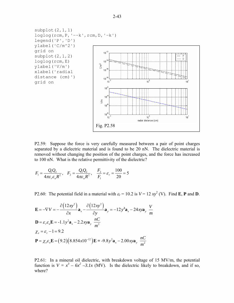
P2.58: MATLAB: A 20 nC point charge at the origin is embedded in Teflon (εr = 2.1). Find and plot the magnitudes of the polarization vector, the electric field intensity and the electric flux density at a radial distance from 0.1 cm out to 10 cm. We use the following equations:

2 , ,4 e o r o

r o

QE P E Dr

Eχ ε ε επε ε

= = =

% M-File: MLP0258 % % Plot E, P and D vs distance r from a point % charge Q at the origin with a dielectric. % % Variables % Q charge (C) % eo free space permittivity (F/m) % r radial distance (m) % Chi electric susceptibility % E electric field intensity(V/m) % D electric flux density (C/m^2) % P polarization vector (C/m^2) % initialize variables Q=20e-9; er=2.1; eo=8.854e-12; Chi=er-1; % perform calculations r=0.001:.001:0.100; rcm=r.*100; E=Q./(4*pi*r.^2); P=Chi*eo*E; D=er*eo*E; % plot data

2-43

subplot(2,1,1) loglog(rcm,P,'--k',rcm,D,'-k') legend('P','D') ylabel('C/m^2')

Fig. P2.58

grid on subplot(2,1,2) loglog(rcm,E) ylabel('V/m') xlabel('radial distance (cm)') grid on P2.59: Suppose the force is very carefully measured between a pair of point charges separated by a dielectric material and is found to be 20 nN. The dielectric material is removed without changing the position of the point charges, and the force has increased to 100 nN. What is the relative permittivity of the dielectric?

1 2 1 2 21 22 2

1

100, , 54 4 r

r o o

Q Q Q Q FF FR R F

επε ε πε

= = = =20

=

P2.60: The potential field in a material with εr = 10.2 is V = 12 xy2 (V). Find E, P and D.

( ) ( )2 212 1212 24 x y x

xy xy VV y yxyx y m

∂ ∂= −∇ = − − = − −

∂ ∂2E a a a a

22-1.1 2.2 r o x y

nCy xym

ε ε= = −D E a a

1 9.2e rχ ε= − =

( )( )12 229.2 8.854 10 -9.8 2.00 e o x y

nCx y xym

χ ε −= = −P E E = a a

P2.61: In a mineral oil dielectric, with breakdown voltage of 15 MV/m, the potential function is V = x3 – 6x2 –3.1x (MV). Is the dielectric likely to breakdown, and if so, where?

2-44

( )23 12 3.1 xMVV x xm

= −∇ = − + +E a

2

26 12, 6, d dxdx dx

= − + = −E E so from 6x – 12 = 0 we find the maximum electric field

occurs at x = 2m. At x = 2m, we have E = -12+24+3.1 = 15.1 MV/m, exceeding the breakdown voltage. 12. Boundary Conditions P2.62: For y < 0, εr1 = 4.0 and E1 = 3ax + 6πay + 4az V/m. At y = 0, ρs = 0.25 nC/m2. If εr2 = 5.0 for y > 0, find E2. E1 = 3ax + 6πay + 4az V/m (g) E2 = 3ax + 20.7ay + 4az V/m (a) EN1 = 6πay (f) EN2 = DN2/5εo = 20.7ay(b) ET1 = 3ax + 4az (c) ET2 = ET1 = 3ax + 4az

(d) DN1 = εr1εoEN1 = 24πεo ay (e) DN2 = 0.92 ay

(e) ( ) ( )21 1 2 1 2 2 1, - , s y N N y s N ND D D D sρ ρ ρ− = − = − =a D D a ai i

9

2 1 2 2

100.25 24 0.9236N s N

nC F nC nCD Dm m m

ρ ππ

−⎛ ⎞= + = + =⎜ ⎟

⎝ ⎠2m

2T

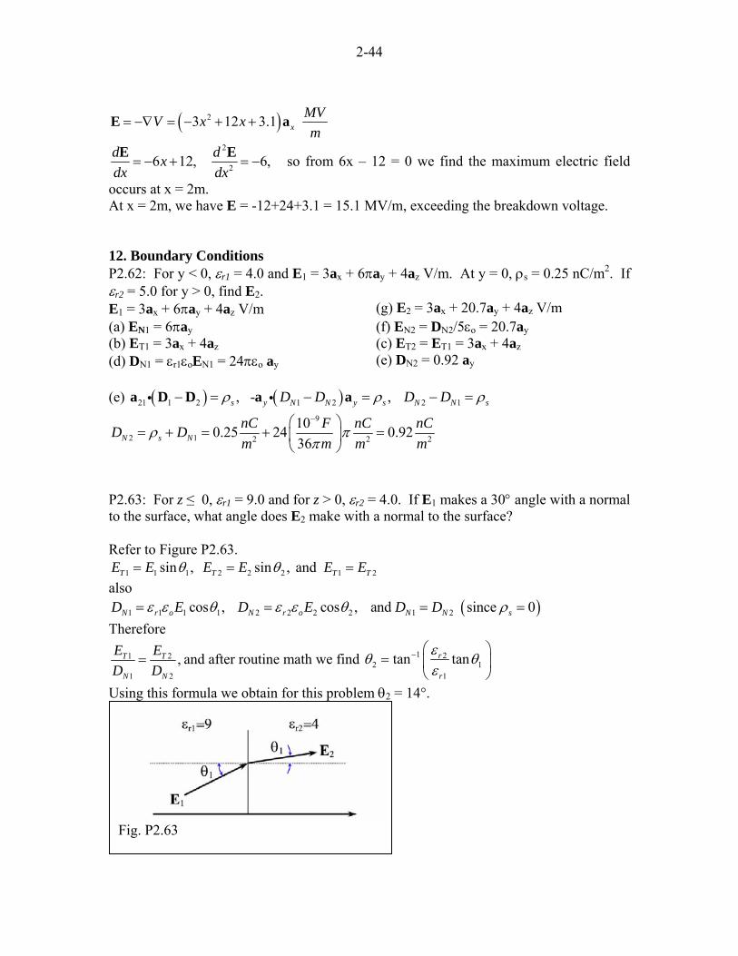
P2.63: For z ≤ 0, εr1 = 9.0 and for z > 0, εr2 = 4.0. If E1 makes a 30° angle with a normal to the surface, what angle does E2 make with a normal to the surface? Refer to Figure P2.63.

1 1 1 2 2 2 1sin , sin , and T T TE E E E E Eθ θ= = = also

( )1 1 1 1 2 2 2 2 1 2cos , cos , and since 0N r o N r o N N sD E D E D Dε ε θ ε ε θ ρ= = = = Therefore

1

1 2

,T T

N N

E ED D

= 2 and after routine math we find 1 22 1

1

tan tanr

r

εθ θε

− ⎛ ⎞= ⎜ ⎟

⎝ ⎠

Using this formula we obtain for this problem θ2 = 14°.

Fig. P2.63

2-45

P2.64: A plane defined by 3x + 2y + z = 6 separates two dielectrics. The first dielectric, on the side of the plane containing the origin, has εr1 = 3.0 and E1 = 4.0az V/m. The other dielectric has εr2 = 6.0. Find E2. We first use gradient to find a normal to the planar surface. Let F = 3x + 2y + z – 6 = 0.

3 2 , and 14,

so 0.802 0.534 0.267 .

x y z

N x y z

F F

FF

∇ = + + ∇ =

∇= = + +

∇

a a a

a a a a

z

1T

1ND

Now we can work the boundary condition problem. ( )1 N1 14 , 0.857 0.570 0.285 .z N N x y= = = + +E a E E a a a a ai

1 1 1 20.857 0.570 3.715 , T N x y z T= − = − − + =E E E a a a E E

1 1 1 22.571 1.710 0.855 , and N r o N o x y z Nε ε ε ⎡ ⎤= = + + =⎣ ⎦D E a a a D

2 22

2

0.429 0.285 0.1436

N NN x

r o oε ε ε= = = + +

D DE a y za a

Finally we have 2 2 2V0.43 0.29 3.8 mT N x y z= + = − − +E E E a a a .

P2.65: MATLAB: Consider a dielectric-dielectric charge free boundary at the plane z = 0. Construct a program that will allow the user to enter εr1 (for z < 0), εr2, and E1, and will then calculate E2. (Just for fun, you may want to have the program calculate the angles that E1 and E2 make with a normal to the surface). % M-File: MLP0265 % % Given E1 at boundary between a pair of % dielectrics with no charge at boundary, % calculate E2. Also calculates angles. % clc clear % enter variables disp('enter vector quantities in brackets,') disp('for example: [1 2 3]') er1=input('relative permittivity in material 1: '); er2=input('relative permittivity in material 2: '); a12=input('unit vector from mtrl 1 to mtrl 2: '); E1=input('electric field intensity vector in mtrl 1: '); % perform calculations

2-46

En1=dot(E1,a12)*a12; Et1=E1-En1; Et2=Et1; Dn1=er1*En1; %ignores eo since it will factor out Dn2=Dn1; En2=Dn2/er2; E2=Et2+En2 % calculate the angles th1=atan(magvector(Et1)/magvector(En1)); th2=atan(magvector(Et2)/magvector(En2)); th1r=th1*180/pi th2r=th2*180/pi Now run the program: enter vector quantities in brackets, for example: [1 2 3] relative permittivity in material 1: 2 relative permittivity in material 2: 5 unit vector from mtrl 1 to mtrl 2: [0 0 1] electric field intensity vector in mtrl 1: [3 4 5] E2 = 3 4 2 th1r = 45 th2r = 68.1986 P2.66: A 1.0 cm diameter conductor is sheathed with a 0.50 cm thickness of Teflon and then a 2.0 cm (inner) diameter outer conductor. (a) Use Laplace’s equations to find an expression for the potential as a function of ρ in the dielectric. (b) Find E as a function of ρ. (c) What is the maximum potential difference that can be applied across this coaxial cable without breaking down the dielectric? (a) Since V is only a function of ρ,

2-47

2 1 0

so

or ln

cylVV

V A

V A B

ρρ ρ ρ

ρρ

ρ

⎛ ⎞∂ ∂∇ = =⎜ ⎟∂ ∂⎝ ⎠

∂=

∂= +

Fig. P2.66

where A and B are constants. Now we apply boundary conditions. BC1: 0 ln , ln

ln

A b B B A b

V Abρ

= + = −

⎛ ⎞

,

∴ = ⎜ ⎟⎝ ⎠

BC2: ( )

( )( )

lnln , ,

ln lna

a aV baV A A V Va ab

b b

ρ⎛ ⎞= = =⎜ ⎟⎝ ⎠

or ( )1.443 ln 100 .aV V ρ= −

(b) 1.443 aVVV ρ ρρ ρ∂

= −∇ = − =∂

E a a

(c)

( )

6max

6

max

1.443 288.5 60 10 ,.00560 10so 208 , 210288.5

aa br

a ab

VE V E x

xV kV V

= = = =

= = ∴ = kV

P2.67: A 1.0 m long carbon pipe of inner diameter 3.0 cm and outer diameter 5.0 cm is cut in half lengthwise. Determine the resistance between the inner surface and the outer surface of one of the half sections of pipe. One approach is to consider the resistance for the half-section of pipe is twice the resistance for a complete cylindrical section, given by Eqn. (2.84). But we’ll used the LaPlace equation approach instead.

Laplace: 2 1 0cylVV ρ

ρ ρ ρ⎛ ⎞∂ ∂

=⎜ ⎟∂ ∂⎝ ⎠∇ = ; here we see V only depends on ρ

So: ; lnV A V A Bρ ρρ

∂= =

∂+ ;

where A and B are constants. Now apply boundary conditions. BC1:

2-48

0 ln ; ln

ln

bV A b B B A

V Abρ

= = + = −

⎛ ⎞= ⎜ ⎟⎝ ⎠

;b

BC2:

( )( )( )

ln ; ;ln

ln

ln

aa

a

VaV A Aab

b

bV Va

b

ρ

⎛ ⎞= =⎜ ⎟⎝ ⎠

=

( )1

lnaVVVa

bρ ρρ ρ

∂= −∇ = − = −

∂E a a

Fig. P2.67

J=σE

( ) ( )0 0

1ln ln

La aV LI d d dz

a bb a

π Vσ π σρ φρ

= = − =∫ ∫ ∫J Si

( )ln5.4 .a

bV aRI L

µπσ

= = = Ω

P2.68: For a coaxial cable of inner conductor radius a and outer conductor radius b and a dielectric εr in-between, assume a charge density v oρ ρ ρ= is added in the dielectric region. Use Poisson’s equation to derive an expression for V and E. Calculate ρs on each plate.

2 1v oVV ρ ρρε ρ ρ ρ ερ

⎛ ⎞ −∂ ∂∇ = − = − =⎜ ⎟∂ ∂⎝ ⎠

so

; ; o oV V Vd dρ ρρ ρ ρ ρρ ρ ε ρ ε ρ ε

⎛ ⎞ ⎛ ⎞∂ ∂ ∂ ∂= = =⎜ ⎟ ⎜ ⎟∂ ∂ ∂ ∂⎝ ⎠ ⎝ ⎠

∫ ∫ o Aρ ρ + , where A is a constant.

; = ; lno o oV A AdV d d V A Bρ ρ ρρ ρ ρ ρρ ε ρ ε ρ ε

∂= + + = + +

∂ ∫ ∫ , where B is a constant.

Now apply boundary conditions: V V at and 0 at a a V bρ ρ= = = = Applying the second one gives us:

( ) ( )ln .oV b A bρ ρρε

= − +

Applying the first one:

2-49

( ) ( )( )

( )ln ;

ln

oa

oa

V baV a b A Ab a

b

aρρ εε

+ −= − + =

Therefore,

( )

( ) ( )ln .ln

oa

oV b a

V ba b

b

ρρρε ρε

+ − ⎛ ⎞= +⎜ ⎟⎝ ⎠

−

ln o o

o

VV Kb

K

bρ ρ

ρ

ρ ρρ ρρ ρ ε ε

ρρ ε

∂ ∂ ⎛ ⎛ ⎞= −∇ = − = − + −⎜ ⎟⎜ ⎟∂ ∂ ⎝ ⎠⎝ ⎠

⎛ ⎞= − −⎜ ⎟

⎝ ⎠

E a

E a

⎞a

where

( )

( )ln

oaV b

Ka

b

aρε

+ −= ,

so ( )

.ln

oa

o

V b a

ab

ρ

ρρεερ

⎡ ⎤⎛ ⎞− + −⎜ ⎟⎢ ⎥⎝ ⎠⎢ ⎥= −⎛ ⎞⎢ ⎥⎜ ⎟⎢ ⎥⎝ ⎠⎣ ⎦

E a

( );

ln

oa

oN s Na sa

V b aD D

aab

ρ

ρρε

aρ ε ρε=

⎡ ⎤⎛ ⎞− + −⎜ ⎟⎢ ⎥⎝ ⎠⎢ ⎥= = = − =⎛ ⎞⎢ ⎥⎜ ⎟⎢ ⎥⎝ ⎠⎣ ⎦

E

( )

ln

oa

oNb sbb

V b aD

abb

ρ

ρρεε ρε=

⎡ ⎤⎛ ⎞− + −⎜ ⎟⎢ ⎥⎝ ⎠⎢ ⎥= −⎛ ⎞⎢ ⎥⎜ ⎟⎢ ⎥⎝ ⎠⎣ ⎦

= E =

P2.69: For the parallel plate capacitor given in Figure 2.51, suppose a charge density

sin2v o

zd

πρ ρ= ⎛ ⎞

⎜ ⎟⎝ ⎠

is added between the plates. Use Poisson’s equation to derive a new expression for V and E. Calculate ρs on each plate.

2-50

( )2

2

sin( ) 2ovzV z d

z

πρρε ε

−−∂= =

∂

( ) ( )2( ) sin cos2 2o odV z z zdz Ad dz

ρ ρπ πε πε

−∂= =

∂ ∫ +

( ) ( )2

2

2 2( ) cos sin2 2o od dz zV z dz A dz Az Bd d

ρ ρπ ππε π ε

= + =∫ ∫ + +

Now apply the boundary conditions:

( )2

2 2

2

220 ; sin ; 2

od

oa d

dVd dV B V Ad Ad d

ρρ π εππ ε

−= = = + =

( )2

2 2

2 2( ) sin 2o dd VzV z zd d

ρ ρππ ε π ε

⎛ ⎞= + −⎜ ⎟⎝ ⎠

od

( )2

2 2

2 2sin 2o d

z zd VV zV zdz z z d

ρ ρππ ε π ε

⎡ ⎤⎛ ⎞ ⎛ ⎞∂ ∂ ∂ ⎛ ⎞= −∇ = − = − + − −⎢ ⎥⎜ ⎟ ⎜ ⎟⎜ ⎟∂ ∂ ∂ ⎝ ⎠⎝ ⎠⎝ ⎠⎣ ⎦E a od a

( ) 2

2cos 2o d

zd Vz

d dρ ρππε π ε

⎛ ⎞= − − +⎜ ⎟⎝ ⎠

E aod

at z = 0, 0

, so N s zD Eε ρ

== = 2

2 .o d os

d V dd

ρ ε ρ ρπ π

− − + =

at z = d, , so N s z dD Eε ρ

== = 2

2 .d os

V dd

ε ρ ρπ

− + =

13. Capacitors P2.70: A parallel plate capacitor is constructed such that the dielectric can be easily removed. With the dielectric in place, the capacitance is 48 nF. With the dielectric removed, the capacitance drops to 12 nF. Determine the relative permittivity of the dielectric.

11 2

2

48; ; 4.012

r o or

A A CC Cd d C

ε ε ε ε= = = = =

P2.71: A parallel plate capacitor with a 1.0 m2 surface area for each plate, a 2.0 mm plate separation, and a dielectric with relative permittivity of 1200 has a 12. V potential difference across the plates. (a) What is the minimum allowed dielectric strength for this capacitor? Calculate (b) the capacitance, and (c) the magnitude of the charge density on one of the plates.

(a) min12 6 ; ( ) 6

0.002 brV kV kE a E

m m m= = =

V

2-51

(b) ( )( )( )12 21200 8.854 10 / 1

5.30.002

r ox F m mAC F

d mε ε µ

−

= = =

(c) ( )( )6; 5.3 10 12 64Q CC Q CV x F VV F

CV

µ−= = = =

P2.72: A conical section of material extends from 2.0 cm ≤ r ≤ 9.0 cm for 0 ≤ θ ≤ 30° with εr = 9.0 and σ = 0.020 S/m. Conductive plates are placed at each radial end of the section. Determine the resistance and capacitance of the section.

2 2 22

1 0; ; V VV r r A Vr r r r r

∂ ∂ ∂⎛ ⎞∇ = = = = − +⎜ ⎟∂ ∂ ∂⎝ ⎠A B , where A and B are constants.

Boundary conditions: r = a, V = 0 and r = b, V = Vb

1 1

1 1ba rV V

a b

⎛ ⎞−⎜ ⎟⎝ ⎠=⎛ ⎞−⎜ ⎟⎝ ⎠

2 2,

1 1 1 1

r

b r r o b r

VVr

V V

r ra b a b

ε ε

∂= −∇ = −

∂− −

= =⎛ ⎞ ⎛ ⎞− −⎜ ⎟ ⎜ ⎟⎝ ⎠ ⎝ ⎠

E a

a aE D

Fig. P2.72

2

2

;1 1

; sin

r o bsb

s

V

ba b

Q dS dS r d d

ε ερ

ρ θ θ φ

−⎛ ⎞−⎜ ⎟⎝ ⎠

= =∫

=

2-52

30 22

2 0 0

12

sin1 1

1.73 10 .

o

r o bb

b

VQ b db

a bx V

πε ε dθ θ φ

−

=⎛ ⎞−⎜ ⎟⎝ ⎠

=

∫ ∫

11.7 ; ; 2.3b

b

QC pF RC RV C

kε εσ σ

= = = = = Ω

P2.73: An inhomogeneous dielectric fills a parallel plate capacitor of surface area 50. cm2 and thickness 1.0 cm. You are given εr = 3(1 + z), where z is measured from the bottom plate in cm. Determine the capacitance. Place +Q at z = d and –Q at z = 0.

, , s z zr o

Q Q QS S

ρε ε

= = − = −D a ES

a

0 0

d d

do z zr o o r

-Q Q dzV d dzS S 0

d

ε ε ε= − = − =∫ ∫E L a ai i

ε∫

evaluating the integral:

( ) ( ) 1

00 0

1 1ln 1 ln 2 3 1 3 3

d d

r

dz dz z czε

= = + =+∫ ∫ m

( )( )( )( )12 2 23 8.854 10 503 19

ln 2 100ln 2o

do

x F m cmSQ mC pV ccm

ε−

⎛ ⎞= = = =⎜ ⎟⎝ ⎠

Fm

P2.74: Given E = 5xyax + 3zaz V/m, find the electrostatic potential energy stored in a volume defined by 0 ≤ x ≤ 2 m, 0 ≤ y ≤ 1 m, and 0 ≤ z ≤ 1 m. Assume ε = εo.

2 2 2

2 1 1 2 1 12 2 2

0 0 0 0 0 0

1 1 25 92 21 25 9 1252

E o o

E o

W dv x y dxdydz z dxdydz

W x dx y dy dz dx dy z dz pJ

ε ε

ε

⎡ ⎤= = +⎣ ⎦

⎡ ⎤= +⎢ ⎥

⎣ ⎦

∫ ∫ ∫

∫ ∫ ∫ ∫ ∫ ∫

E Ei

=

P2.75: Suppose a coaxial capacitor with inner radius 1.0 cm, outer radius 2.0 cm and length 1.0 m is constructed with 2 different dielectrics. When oriented along the z-axis, εr for 0° ≤ φ ≤ 180° is 9.0, and for 180° ≤ φ ≤ 360° is 4.0. (a) Calculate the capacitance. (b) If 9.0 V is applied across the conductors, determine the electrostatic potential energy stored in each dielectric for this capacitor. (a) a coaxial line,

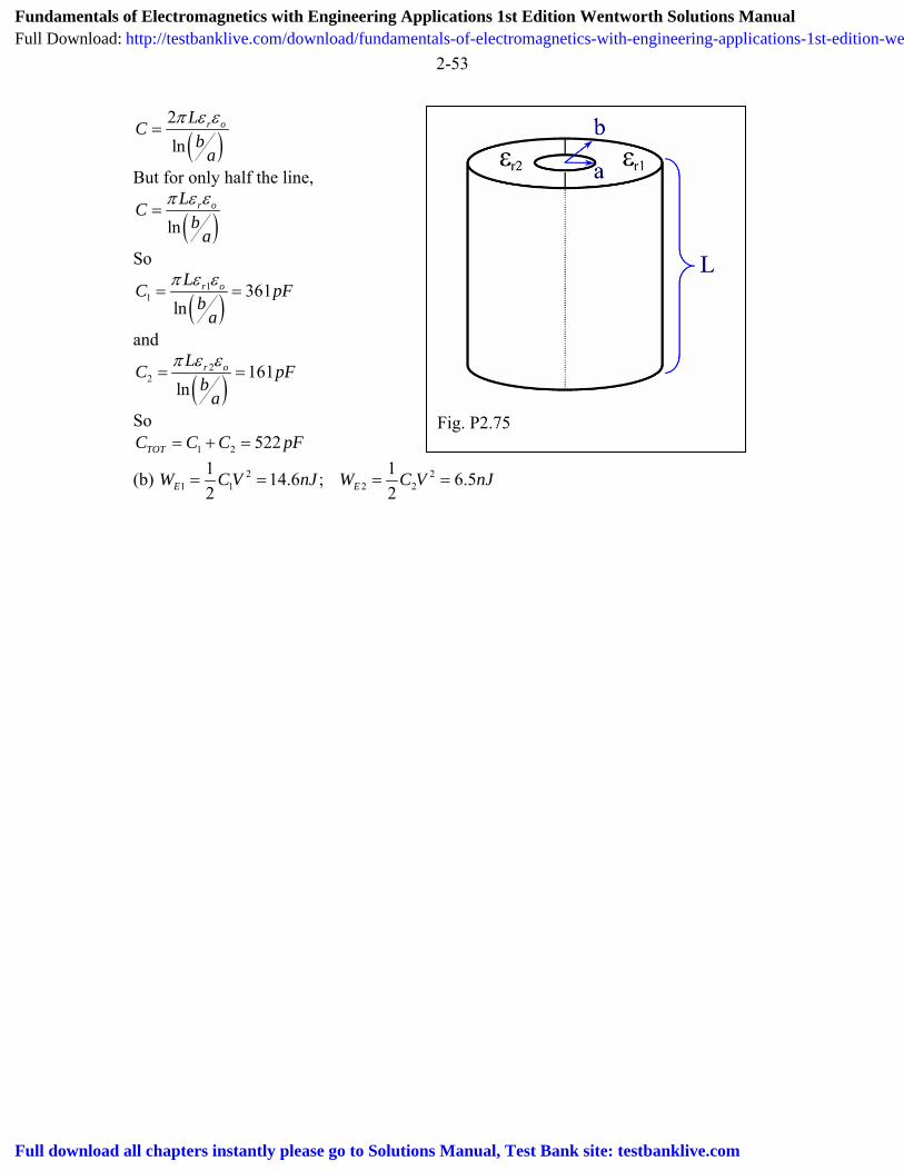
2-53

Fig. P2.75

( )2ln

r oLCb

a

π ε ε=

But for only half the line,

( )lnr oLC

ba

π ε ε=

So

( )1

1 361ln

r oLC pb

aFπ ε ε

= =

and

( )2

2 161ln

r oLC pb

aFπ ε ε

= =

So 1 2 522TOTC C C p= + = F

(b) 2 21 1 2 2

1 114.6 ; 6.52 2E EW C V nJ W C V nJ= = = =

Fundamentals of Electromagnetics with Engineering Applications 1st Edition Wentworth Solutions ManualFull Download: http://testbanklive.com/download/fundamentals-of-electromagnetics-with-engineering-applications-1st-edition-wentworth-solutions-manual/

Full download all chapters instantly please go to Solutions Manual, Test Bank site: testbanklive.com