solutions manual: part v welfare resources (by author)/m... · the line convex, and the one below...

For use with Robert I. Mochrie, Intermediate Microeconomics, Palgrave, 2016

Solutions Manual: Part V

Welfare

Summary answers to the ‘By yourself’ questions

For use with Robert I. Mochrie, Intermediate Microeconomics, Palgrave, 2016 Chapter 20 X20.1 Given that the endowments represent Liling’s and Maya’s total wealth, explain why the

expressions on the left-hand side of Expression 20.2 cannot both be positive. Were both expressions positive, then there would be a move up and to the right in the diagram. Liling would consume more carrots and more beans; and Maya would consume less of both. So, assuming that preferences are well behaved, Liling would be better off and Maya would be worse off, meaning that Maya would not agree to the new division.

X20.2 Define the marginal rate of substitution for Liling and Maya at the endowment, E. Explain

how the difference in values means that trade is possible. For both Liling and Maya, the marginal rates of substitution are the slopes of the tangents to their indifference curves. We see that Maya’s indifference curve is steeper than Liling’s, so that she is willing to give up more carrots than Liling to acquire a set quantity of additional

beans. Liling and Maya could agree to any exchange rate : MRSL > - > MRSM. X20.3 In Figure 20.2, the endowment is at the lower-right corner of the lens. Under what

conditions would the endowment be at the upper-left corner of the lens? What would be the outcome of trade in this case?

We now require Liling’s indifference curve to be steeper than Maya’s, so that MRSM > - > MRSL.

X20.4 Use Expression 20.2 to obtain an expression for the relative price of broad beans (the rate

at which Maya gives up consumption of carrots in order to increase consumption of broad beans). The relative price will be the ratio of the increase in consumption of broad beans to the

increase in consumption of carrots. We obtain EL

TL

EL

TL

cc

bb

.

X20.5 Suppose that at the division, E, Liling and Maya were to have the same marginal rate of

substitution. Sketch an Edgeworth box showing this outcome. What do you conclude about the possibility of exchange? In the Edgeworth box, we begin by drawing a straight downward-sloping line that will be the common tangent. We then draw two curves, both downward-sloping, with the one above the line convex, and the one below the line concave. We draw these lines so that each has a single point of tangency between each curve and the line; and so that the point of tangency is common to both curves. We note that there is no area defined by the intersection between the curves, and so there are no divisions of the endowment where both Liling and Maya are better off than at the point of tangency. This implies that there is no possibility of trade between Liling and Maya.

X20.6 How likely do you consider it to be that Liling would accept the division of goods at F?

It is possible, but we note that Liling is no better off than at E, so that she has no strong reason to agree to the new division.

X20.7 Explain why division G is Pareto efficient, and discuss whether or not you consider it likely

that it will be the outcome of exchange. G is Pareto efficient since the indifference curves through this division share a common tangent. At this division, Maya is no better off than at the initial endowment, E, so it is unlikely that she would agree to the division.

For use with Robert I. Mochrie, Intermediate Microeconomics, Palgrave, 2016 X20.8 The contract curve is sometimes defined as the portion of the Pareto set between F and G.

Why might this be a useful definition? [Hint: Consider peoples’ willingness to agree to any division of the endowment.] Between F and G, both Liling and Maya are better off than at the endowment E. Since all points on the contract curve share a common tangent, there is no possibility of further Pareto improvements. It is therefore possible that Liling and Maya might agree to any of these divisions, with neither being able to propose an alternative division in which both would be better off.

X20.9 Suppose that Maya and Liling consider broad beans and carrots to be perfect

complements, with their preferences represented by the utility function, U: U(bi, ci) = min(bi, ci). The total quantities of broad beans and carrots in their total endowment are equal.

a) Explain why, in any division in which bL = cL, their indifference curves just touch. We know that with both Liling and Maya treating the goods as perfect complements, their preferences across divisions can be expressed by a set of L-shaped indifference curves. For Liling, the vertices are on the line bL = cL. On this line, bM = b – bL = c – cL = cM, so that the vertices of Maya’s indifference curves also lie on this line. At every point on the line, bL = cL, any downward-sloping line is a common tangent to the indifference curves that meet at this point.

b) Suppose instead that Liling grows carrots and Maya grows broad beans. Using a diagram, show that if Maya can determine the division of the endowment, she can take all of Liling’s carrots and offer no broad beans in return. With Maya growing broad beans, but taking all of Liling’s carrots, Liling is no worse off than at the initial division, so that the Pareto efficiency condition is met by trade.

c) Again, using the diagram, show that it is possible for Maya and Liling to trade to any division for which cL = bL. From parts a) and b), we see that the Pareto set is represented in the Edgeworth box by the line, OLOM, running from the bottom left to the top right corners (that is from the origin of Liling’s measurement to the origin of Maya’s measurement); and all divisions in the Pareto set are feasible in the sense that neither Liling nor Maya would be worse off after trade than before. The whole of the line is the contract curve.

X20.10 Now suppose that Maya and Liling consider carrots and broad beans to be perfect

substitutes. However, while Maya would substitute 1 kg of broad beans for 1 kg of carrots, Liling would swap 2 kg of broad bean for 1 kg of carrots.

a) Draw an Edgeworth box showing indifference curves, given that they wish to divide 12 kg of carrots and 20 kg of broad beans, and that Maya starts with all of the carrots, and Liling with all of the broad beans. On your diagram, indicate the region within which they might trade. We draw the Edgeworth box, measuring the endowment of broad beans on the horizontal axis and the endowment of carrots on the vertical axis, so that the dimensions of the box are 20x12. We denote the bottom-left hand corner as OL, from which Liling’s consumption is measured; and the top-right corner as OM, from which Maya’s consumption is measured. Then the initial endowment, E, is located at the bottom-right corner of the box. For Liling, the indifference curve through point E has the equation bL + 2cL = 20, while for Maya, it has equation bM + cM = 12.


Liling’s indifference curve is a line meeting the left-hand edge of the box, (0, 10), while Maya’s is a line meeting the top edge of the box at (8, 12). We see that Maya’s indifference curve is steeper than Liling’s, so that the feasible set for trade is the area between them.

b) Assume instead that their initial endowments are (bLE, cL

E) = (12, 6) and (bME, cM

E) = (8, 6). Draw another Edgeworth box, and mark on it this endowment, E. Sketch the indifference curves through the endowment, and indicate the region within which trade might occur. In this case, the initial endowment, E, is located at the point (bL

E, cLE) = (12, 6). For Liling, the

indifference curve through point E has the equation bL + 2cL = 24, while for Maya, it has equation bM + cM = 14. Liling’s indifference curve is a line meeting the top of the box at (0, 12), while Maya’s is a line meeting the top edge of the box at (6, 12). As before, Maya’s indifference curve is steeper than Liling’s, so that the feasible set for trade is the area between them.

c) What is the range of terms of trade which Maya and Liling might agree? The terms of trade will be such that both Maya and Liling are better off after trade. We

define the relative price, , as the opportunity cost of beans, defined so that MRSM > > -

MRSL; or so that -0.5 > > - 1.

d) Under what conditions might Liling end up with all of the carrots? This will happen if the exchange line is steep enough so that it passes through the top edge of the box.

X20.11 Suppose that Maya and Liling have preferences represented by the utility function,

U: 32

31

, iiii cbcbU . The initial endowment, E: (bLE, cL

E) = (90, 0) and (bME, cM

E) = (30, 120).

Assume that they agree to trade 1 kg of carrots for 2 kg of broad beans. a) What is the opportunity cost of 1 kg of broad beans?

The opportunity cost, = –0.5.

b) Write down expressions for their marginal utility functions and their (common) marginal rate of substitution, MRS. We obtain marginal utilities by partially differentiating U with respect to the quantity of each of the goods in the consumption bundle.

So marginal utility of beans, MUB = 32

i

i

i b

c

31

bU

; and marginal utility of carrots, MUC =

The marginal rate of substitution is (minus 1 times) the ratio of marginal utilities; MRSi =

i

i

c

b

32

b

c

31

MU

MU

b2

c

31

i

i

32

i

i

C

B .

c) Show that MRS = –0.5 whenever b = c. What do you conclude about the composition of

the most preferred, affordable consumption bundle?

If MRSi = -0.5, then 21

b2

c

i

i , so ci = bi. We note that when bi = ci, Liling and Maya have the

same marginal rate of substitution; and note that for the total endowment (b, c) = (120, 120), then if bL = cL, bM = 120 – bL = 120 – cL = cM; so that the conditions for Pareto efficiency are satisfied when bL = cL; and the Pareto set consists of all allocations (bL, cL): bL = cL.

31

i

i

i c

b

32

cU


d) Confirm that the division H: (bLH, cL

H) = (30, 30) and (bMH, cM

H) = (90, 90) is feasible, given the terms of trade; and that Liling’s and Maya’s indifference curves through H both have

gradient = –0.5. To reach division H from the initial endowment, E, Liling gives up 60kg of beans, and acquires 30kg of carrots; Maya acquires 60kg of beans in exchange for 30kg of carrots. At division H, the conditions for Pareto efficiency are satisfied, with beans being exchanged for carrots at the agreed relative price.

e) Sketch an Edgeworth box showing the endowment point; the terms of trade line; the indifference curves passing through the endowment point, E; and the indifference curves passing through the final division, H. In an Edgeworth box with dimensions 120x120, we measure the division of beans on the horizontal axis, and division of carrots on the vertical, measuring the quantity available to Liling of each from the bottom left corner. The initial endowment E: (90, 0) therefore lies on the bottom edge of the box, three-quarters of the way from the left side to the right side of the box. The terms of trade line starts from point E, and has slope -0.5, so that it passes through point H(30, 30). At this final division, the indifference curves for Liling and Maya (which are downward sloping and convex to their respective origins, approaching but never touching the axes against which they are measured) both have gradient -0.5, so that the terms of trade line forms a common tangent.

X20.12 In Figure 20.6, we suggest that Lukas and Michael will divide the endowment equally.

a) Confirm (from Expression 20.10) that Michael’s preferred bundle is half of the endowment

if the relative price, bc .

We know that Michael’s optimal bundle 2c

2c

MM ,*c*,b

. So with the relative price = bc,

the result follows. 2c

2b

MM ,*c*,b

b) Demonstrate that when the relative price, bc , Lukas’s most preferred affordable

bundle, 22

,**, cbcb .

If the relative price = bc, then for Lukas, MRSL =

L

L

b

c = bc. Then cMb = bMc; and for the

feasibility constraint to be satisfied, bcbL + cL = c. Then cL =

2c

b

b

b

bbcc ML

; and it is easy to

confirm that bL = 2b

.

c) Explain why we can write Lukas’s problem as having two constraints:

LL cb ,

max (bL cL)½: cL = b

c(b - bL) and [(b – bL)(c – cL)]

½ = 21

21 bc . Form the Lagrangean, ,

required to solve the problem. Lukas’s problem has the two constraints of affordability and feasibility. It has to be possible for Lukas and Michael to trade to the equilibrium. Michael has to be willing to accept the outcome of the trade, and so must be no worse off than at his optimum.

We write the Lagrangean, .ccbbbccbbcbccb 5.0LL

5.0

21

LL5.0

LL

d) By obtaining the first-order conditions, confirm that 2* c

Lc .

The first-order conditions for an optimum can be written as

.05.05.0

5.05.0

L

L

L

L

L bb

cc

b

c

b c


.05.05.0

5.05.0

L

L

L

L

L cc

bb

c

b

c b

.0cbbcbc LL

.0ccbbbc 5.0LL

5.0

21

We see from the last two expressions that (b – bL)c = bcL, so we can repeat the argument. Since

c – cL = Lbc b , we can rewrite the last condition as bcbbb4 Lb

cL , so that 4(b – bL)bL = b2.

This simplifies to (b – 2bL)2 = 0, so that bL = 2

b. The result then follows by substitution.

X20.13 Assume that Rachel’s maximization problem can be written as:

0:, 1

,

max

RE

RRE

RRRRRcbccbbcbcbU

RR

a) By forming the Lagrangean or otherwise, confirm that Rachel’s most preferred, affordable

bundle (bR*, cR*) has the characteristic: *

1

* RR cb

.

We write the Lagrangean, : = bRcR

1 - + [(bRE – bR) + (cR

E – cR)] We obtain first-order conditions for the maximum:

01

b

c

b R

R

R

; 01R

R

R c

b

c

; and 0ccbb RE

RRE

R

Taking the first two, we see that

R

R

R

R

c

b1

b

c1

. The result follows immediately

from cross-multiplying terms.

b) Hence or otherwise, demonstrate that Rachel’s most preferred affordable bundle is :**, RR cb

ER

ER

cERRR cb1,b*c*,b

ER

We write R1

R bc

, and since (bR

E – bR) + (cRE – cR) = 0, we can write

ER

ERRR

1cbbb1

; and the result follows immediately.

c) Show that as the relative price, , increases, cR increases, but bR decreases.

By partial differentiation, we see that 02

ERR cb

, but that 0b1 E

RcR

d) Write an expression for cR* in terms of bR*. (This is the equation of Rachel’s price offer

curve.)

We see that it is possible to extract a common factor, bRE + cR from the expressions for bR*

and cR*. This gives us cR* =

*bR1

.

X20.14 Assume that Rachel continues to solve the problem in X20.13, but with the expenditure

share parameter, 31a , and initial endowments (bR

E, cRE) = (bS

E, cSE) = (12, 12).

a) Obtain an expression for Rachel’s optimal consumption bundle in terms of the relative

price, .

We apply the expressions obtained from X20.13: ER

ER

cERRR cb1,b*c*,b

ER

.

Then

18,141212,12*c*,b 13212

31

RR .


b) Show that if > 0.5, Rachel will want to trade some of her broad beans for more carrots.

If = ½, it is easy to confirm that (bR*, cR*) = (12, 12) = (bRE, cR

E), so that Rachel can do no

better than by consuming her endowment. Given that bR* is decreasing in , and that cR* is

increasing in , it follows that if > 0.5, then Rachel will give away some beans, and demand more carrots.

c) Evaluate the expression in (a) for Rachel’s optimal consumption bundle for relative prices

= 0.125, 0.25, 0.5, 1, 2, and 4. Are all of these choices feasible?

0.125 0.25 0.5 1 2 4

bR* 36 20 12 8 6 5

cR* 9 10 12 16 24 40

We see that when the relative price, = 2, cR* = 24, so that Rachel wishes to consume all of

the carrots. With cR* increasing in , this is the maximum possible value of the relative price; for higher prices, the price offer curve will lie outside the box.

Although it is not shown in the table, we note that when = 0.2, bR* = 24. In this case, Rachel wishes to consume all of the beans in the endowment and, as before, with bR*

decreasing in , this is the minimum possible value of the relative price; for lower prices, the price offer curve will lie outside the box.

d) Sketch Rachel’s price offer curve. Plotting these points in an Edgeworth box with dimensions 24x24, we see that Rachel’s price offer curve is downward sloping and convex to OR. It intersects the top edge of the box at the division (bR, cR) = (6, 24), where MRS = -2, passes through the division (12, 12), and intersects the right edge of the box at the division (24, 6), where MRS = -0.2.

X20.15 Repeat X20.14 but for Sonja, whose utility function we write as 31

32

, SSSS cbcbU .

We are able to write Sonja’s preferred division, given the relative price as (bS*, cS*):

ER

ER

cERSS cb,b1*c*,b

ER

, which with the given parameterization becomes

14,181212,12*c*,b 13112

32

SS .

Replicating the table of preferred consumption bundles from X20.14:

0.125 0.25 0.5 1 2 4

bS* 72 40 24 16 12 10

cS* 4.5 5 6 8 12 20

We note that it would not be feasible for the value of to be very small: from the table, and knowing that Sonja’s demand for beans in her preferred division, bS* is decreasing in the

relative price, , we require bS* 0.5. Although we have not shown this in the table, it is

straightforward to show that if > 5, then cS* > 24, so that Sonja would then demand more than the total endowment of carrots.

X20.16 Given the endowments and utility function in X20.14 and X20.15, confirm that at the

division J: (bRJ, cR

J) = (8, 16); (bsJ, cs

J) = (16, 8) with relative price = 1, Rachel and Sonja maximize their utilities and both markets clear. We see that by adding up the demands that both markets clear, the demand for both beans and carrots equals the total endowment.

X20.17 Suppose that the relative price increases, so that = 2. Find Rachel’s and Sonja’s most preferred, feasible consumption bundles. Explain why these are not consistent with an equilibrium division.


When = 2, (bR*, cR*) = (6, 24); and (bS*, cS*) = (12, 12). The total demand for carrots is 36, so that there is excess demand for them; and the total demand for beans is 18, so that there is excess supply.

X20.18 Repeat X20.17, but with the relative price decreasing so that = 0.5. Without carrying out

any further calculations, characterize the nature of the outcome for = 0.5. We have seen that when the relative price is above the market clearing price, there is excess demand for carrots, and excess supply of beans. We therefore expect that for a relative price less than the market clearing price, there will be excess supply of carrots and excess demand for beans.

[Check: When = 0.5, (bR*, cR*) = (12, 12); and (bS*, cS*) = (24, 6). The total demand for carrots is 18, so that there is excess supply of them; and the total demand for beans is 36, so that there is excess demand.]

X20.19 Continuing to use the endowments and utility functions in X20.14 and X20.15, suppose

that Rachel initially proposes = 2. a) Confirm that Sonja will not wish to trade, but that Rachel would wish to acquire Sonja’s

endowment of carrots. This follows directly from calculations that we have completed already. Sonja demands her initial endowment, while Rachel demands the bundle (bR, cR) = (6, 24), which includes the total endowment of carrots.

b) Calculate the excess demand for carrots and the excess supply of broad beans. Again, from previous calculations, we see that there is an excess demand for carrots, cR + cS -24 = 12 and excess supply of beans, 24 – (bR + bS) = 6.

c) Repeat parts (a) and (b), assuming firstly that Sonja proposes a revised relative price, =

1.5, and then that Rachel proposes a further revision, = 1.25. We present the results in a table, in which the first four columns show Rachel and Sonja’s demands for beans and carrots, and the next two show the excess demand for beans and carrots.

bR* bS* cR* cS* bX cX bX + cX

2 6 12 24 12 -6 12 0

1.5 3

20 3

40 20 10 -4 6 0

1.25 7.2 14.4 18 9 -2.4 3 0

1 8 16 16 8 0 0 0

We note that as the relative price falls towards the market clearing price, there is a reduction in the excess supply of beans and the excess demand for carrots.

X20.20 To prove some important results in general equilibrium theory, it is often convenient to

rely upon Walras’ Law: that the sum of values of excess demand across markets must be equal to zero.

a) Confirm that Walras’ Law is satisfied in X20.19, so that at each relative price, the value of the excess demand for carrots is also the value of the excess supply of broad beans. This is straightforward: we multiply the excess demand for beans by the relative price, and add the excess demand for carrots. In all cases in the table in X20.19, we see that this condition is satisfied.


b) Given that Rachel and Sonja share a single feasibility constraint, use an Edgeworth box to demonstrate that if the market for carrots clears, the market for broad beans must also clear. Suppose otherwise. Then it would be possible to draw an Edgeworth box, with dimensions representing the endowment of beans and carrots, and Rachel’s share of the endowment in any division measured from the bottom left corner (with the distance from the left edge representing the quantity of beans, and the distance from the bottom the quantity of carrots in her consumption bundle), with the feasibility constraint shown as a downward sloping straight line, passing through the endowment. There are two points shown on the feasibility constraint, one Rachel’s preferred division, and the other Sonja’s preferred division, where the quantity of carrots available to Rachel would be the same in both, but the quantity of beans would be different. This contradicts the assumption that the line has a negative gradient, since as the quantity of beans increases, the quantity of carrots in the division must decrease.

c) Show that if there is a Walrasian equilibrium, the division must also be Pareto-efficient. Continuing to think about the Edgeworth box analysis, if there is a Walrasian equilibrium then the indifference curves passing through that division share a common tangent, and so there is no possibility of further, mutually beneficial trade for Rachel and Sonja: if Rachel increases her utility, it will be at some cost to Sonja (and vice versa). This division is therefore Pareto-efficient.

X20.21 Using the results of X20.16, explain why we can be certain that the Walrasian equilibrium

J1 will be achieved through an exchange that begins from any division on the line bR + cR = 24. In X20.16, we have seen that it is possible to trade to the equilibrium division (bR*, cR*, bS*, cS*) = (8, 16, 16, 8) from a single point on this line. It must therefore be possible to reach this division from any point on this line.

X20.22 Assume that Rachel and Sonja have identical Cobb-Douglas preferences over consumption

bundles containing broad beans and carrots:

32

31

32

31

SSSSRRRR cbc,bU;cbc,bU

with a total of 24 kg of both goods in every division. a) By partial differentiation, or otherwise, show that if Sonja has to meet a payoff target VS :

VS (12), Rachel will propose a division in which bR = cR.

We write the Lagrangean, , for the constrained optimization as:

12c24b24cb,c,b 32

31

32

31

RRRRRR

Partially differentiating with respect to bR and cR, we obtain the first-order conditions:

032

R

R32

R

R

R b24

c24

3b

c

31

b

, so that 3

2

R

R32

R

R

c24

b24

b

c

; and

031

R

R31

R

R

R c24

b24

32

c

b

32

c

, so that 3

1

R

R31

R

R

b24

c24

c

b

. Then since the right hand side of these

expressions must be equal, (24 – cR)bR = cR(24 – bR), and bR = cR.

b) Confirm that whatever division Rachel proposes, with bR = cR, her marginal rate of

substitution, 5.0

R

R

R

R

c

Ub

U

.


For Rachel, marginal rate of substitution, MRS : MRS(bR, cR) =

R

R

c

b

32

b

c

31

cU

bU

C

B

b2

cMU

MU31

R

R

32

R

R

R

R

; and so the result follows directly, given bR = cR.

c) Hence confirm that if Sonja insists on receiving a payoff VS, she will just meet that target if

the initial endowment lies on the line 36c2b RR .

We require Sonja to obtain payoff VS = 12, and confirm that where Rachel proposes the

division (bS, cS) = (24 – bR, 24 – cR) = (12, 12), Sonja obtains payoff VS = 32

31

12.12 = 12; so Sonja just meets her target. We also note that for Sonja, MRSS(12, 12) = -½, since she and Rachel have the same utility function; so when they divide the allocation equally, Sonja is just able to achieve her target payoff while Rachel maximizes her utility subject to that constraint. In terms of an Edgeworth box with dimensions 24x24, reflecting the total endowment, and with Rachel’s allocation of beans measured along the bottom edge from the left hand corner, and her allocation of carrots measured along the left edge, we draw in the indifference curves passing through the division K: (bR. cR; bS, cS) = (12, 12; 12, 12) as convex curves, which have a common tangent at K, with gradient -0.5. We can therefore write the equation of the tangent as (cR – 12) = -0.5(bR – 12), so that bR + 2cR = 36.

X20.23 Rachel and Sonja seek to maximize their utilities, which have the same form as in X20.22.

Suppose that Sonja has a utility target VS = 10. Rachel’s endowment ER = (18, 12); Sonja’s endowment ES = (6, 12). Sketch a diagram showing (1) the initial endowment; (2) the Pareto set; (3) the relative price at which they will trade; and (4) the indifference curves (for Rachel only) at the initial endowment and after trade. We draw here on what we have already found out about this situation in X20.22. Drawing an Edgeworth box with dimensions 24x24, reflecting the total endowment, and with Rachel’s allocation of beans measured along the bottom edge from the left hand corner, and her allocation of carrots measured along the left edge, we denote the endowment E: (bR

E, cRE; bS

E, cS

E) = (18, 12; 6, 12) as a point ¾ of the distance from the left to the right edges and midway between the top and the bottom edges. We know that from this endowment, given the

relative price = -0.5, Rachel and Sonja will agree to trade to a division K1: (bR. cR; bS, cS) where bR = cR and bS = cS, with Rachel giving up 2kg of beans for every 1kg of carrots that she obtains from Sonja. This implies that Rachel will trade 4kg of beans for 2kg of Sonja’s carrots; Sonja ends up with 10kg of beans and carrots, and Rachel ends up with 14kg of each. Rachel ends up better off because she has a larger proportion (in terms of value) of the endowment.

X20.24 Confirm that irrespective of her initial endowment, when Rachel’s price offer curve

intersects the Pareto set, bR = cR, her marginal rate of substitution, MRSR = -0.5. This follows directly from the argument of X20.22b).

X20.25 What might be the policy implications of this capacity of an exchange economy to reach a

competitive equilibrium from any initial division of endowments? This suggests that if we are concerned about the outcome, it is possible to cause some variation in it by changing the initial endowment, rather than prices within the economy. This suggests that lump-sum taxes might be preferable to proportional taxes based on activity, which will change prices.

X20.26 Using Figure 20.12, confirm that compared with the competitive equilibrium, J*, Rachel

secures a larger share of the final division and so a higher utility when she is able to choose

the relative price *.


We note that Rachel’s indifference curve, ICRM intersects the Pareto set above and to the right

of the intersection of Sonja’s price offer curve, PS, with the Pareto set. The competitive equilibrium would occur at the latter intersection, so Rachel must be better off when able to choose the price.

X20.27 We can write Rachel’s problem formally as:

E

SE

SSSSSSc,b

maxSS

ES

ESS

ES

ESSR

max

cbcb:c,bU:*c*,b

,c,b*cc,,c,b*bbU

SS

where

,

a) Set out Rachel’s problem for the now familiar case in which the endowment of 24 kg of broad beans and 24 kg of carrots is divided equally between them, when Rachel’s utility

function 32

31

, RRRRR cbcbU , and Sonja’s utility function 31

32

, SSSSS cbcbU .

Sonja’s constraint can be simplified substantially in this case, since bSE = cS

E = 12. She wishes

to maximize her utility subject to the constraint that bS + cS = 12(1 + ). We rewrite Rachel’s problem as

112cb:c,bU:*c*,b where ,*c24,*b24U SSSSSc,b

maxSSSSR

max

SS.

b) Solve Sonja’s maximization problem, defining her demands bS and cS in terms of the

relative price, . Note: you can use the expressions for demands obtained in Chapter 9, to simplify calculations.

We write the Lagrangean, , for the constrained optimization as:

`SSSSSS cb112cb,c,b 31

32

Partially differentiating with respect to bS and cS, we obtain the first-order conditions:

031

S

S

S b

c

32

b

,and 0

32

S

S

S c

b

31

c

, so that 3

2

S

S31

S

S

c

b

31

b

c

32

. From the latter

equality, 2cS = bS.

In addition, in the last first-order condition, 0cb112 `SS

, substituting for

bS, 12(1 + ) = 3cS, so that we obtain

14,8*c*,b

1SS .

c) Hence, solve Rachel’s maximization problem, defining the relative price, M, so that Rachel maximizes her utility.

From b), we are able to simplify Rachel’s problem further:

54,28U 1R

max. This

becomes 32

31

5428U 1R

max

, and on differentiating, we obtain the first-order

condition: 054285428 31

31

32

32

2

R 1381

3

8d

dU

.

This simplifies to

11 28542 , so that 5 - = 42 - 2, and 42 - - 5 = 0. Applying

the quadratic formula, we obtain 25.18

811

.

d) Compare the outcome in parts (b) and (c) with the Walrasian equilibrium when prices are

set competitively, confirming that with Rachel able to set the relative price, it is now higher, that Rachel’s share of the endowment (and so her payoff) has increased, but that Sonja is worse off. Confirm that the monopoly outcome is not Pareto optimal.


From X20.16, we know that the competitive equilibrium division is J1: (bR*, cR*; bS*, cS*) =

(8, 16; 16, 8), with the competitive equilibrium price, * = 1. Here we see that Rachel

chooses a relative price = 1.25, which is greater than in equilibrium. We do not perform all of the calculations here, but substituting back into the solution of part b), we see that Sonja chooses the bundle (bS, cS) = (14.4, 9), so that Rachel is able to consume the bundle (9.6, 15). There is less trade than we would expect there to be in the Pareto efficient outcome, and we

see for Rachel MRS(9.6, 15) 1.25, so that the requirement MRSR = MRSS = is not satisfied. X20.28 Repeat X20.27, but replacing the utility functions and endowments:

a) Rachel: utility, 32

31

RRRRR cbc,bU , endowment ER = (18, 12);

Sonja: utility, 32

31

SSSSS cbc,bU , endowment ES = (6, 12).

Sonja’s constraint can again be simplified, given the endowments. She wishes to maximize

her utility subject to the constraint that bS + cS = 6(2 + ). We rewrite Rachel’s problem as

26 where ,2424 32

31

32

31

SSSSc,b

maxSSSS

max cb:cb:*c*,b*c*bSS

.

We write the Lagrangean, , for Sonja’s constrained optimization as:

`SSSSSS cbcb,c,b 2632

31


032

31

S

S

S b

c

b ,and 031

32

S

S

S c

b

c , so that 31

32

32

31

S

S

S

S

c

b

b

c . From the latter

equality,

cS = 2bS.

In addition, in the last first-order condition, 026

`SS cb

, substituting for cS,

6(2 + ) = 3bS, so that we obtain 2412 2 ,*c*,b SS .

We now return to Rachel’s problem, which we simplify as: 32

31

24241224 2

max,

or

32

31

41622 4

max. On differentiating, we obtain the first-order condition:

04162241622 31

31

32

32

24

384

34

d

dUR.

This simplifies to 21 1142 , so that 4 - = 112 - 2, and 112 - - 4 = 0. Applying

the quadratic formula, we obtain 600221771 .

.

b) Rachel: utility, 21

21

, RRRRR cbcbU , endowment ER = (24, 0);

Sonja: utility, 21

21

, SSSSS cbcbU , endowment ES = (0, 24).

Sonja’s constraint can again be simplified, given the endowments. She wishes to maximize

her utility subject to the constraint that bS + cS = 24. Note that since Sonja has no endowment of good B, the value of her endowment is constant, and does not depend on the relative price that Rachel chooses. We rewrite Rachel’s problem as

24 where ,2424 21

21

21

21

SSSSc,b

maxSSSS

max cb:cb:*c*,b*c*bSS

.

We write the Lagrangean, , for Sonja’s constrained optimization as:


`SSSSSS cbcb,c,b 2421

21


021

21

S

S

S b

c

b ,and 021

21

S

S

S c

b

c , so that 21

21

21

21

S

S

S

S

c

b

b

c . From the latter

equality,

cS = bS.

In addition, in the last first-order condition, 024

`SS cb

, substituting for bS,

24 =2cS, so that we obtain 1212 ,*c*,b SS .

We now return to Rachel’s problem, which we simplify as: 21

21

1224 12

max

, or 21

1212

max.

On differentiating, we obtain the first-order condition:

02 505121

2 12

616..

R

d

dU

. This is

a rather complicated expression, but we can show that it can only be evaluated for value of

> 0.5, and that the derivative is decreasing in , but always positive, so that Rachel will set as

large a value as possible. As , (bS*, cS*) (0, 12). Rachel takes half of Sonja’s endowment, offering as little as possible in return. Given the form of the utility functions, and the extent of Rachel’s monopoly power, this should seem intuitively reasonable

For use with Robert I. Mochrie, Intermediate Microeconomics, Palgrave, 2016 Chapter 21 X21.1 Suppose Robinson has a diminishing marginal product of labour, while he requires an

increasing rate of compensation for his labour, on the basis that his preferences over combinations of leisure time and fish are well behaved.

a) Sketch a diagram representing the total quantity of fish that Robinson can catch (as a function of labour time); and (at least) three separate indifference curves representing levels of preference over combinations of labour time and fish, one of which just touches the total quantity curve. Drawing a diagram with Robinson’s hours of work measured on the horizontal axis and the number of fish that he catches measured on the vertical axis, we draw an upward-sloping concave curve that starts from the origin. This output curve represents the total quantity of fish that Robinson catches. We also draw three upward-sloping convex curves, which begin from some point on the vertical axis, and one of which is drawn so that there is some point of common tangency between this curve and the output curve. These convex curves are effectively indifference curves, drawn on the basis that Robinson trades off effort against catching fish.

b) Define the agreed wage w as the number of fish that Mr Crusoe gives Robinson per hour of

labour time. Assume that Mr Crusoe will also pay Robinson a retainer – a quantity of fish, F0 = F(0), in addition to the wage paid for fishing. Sketch straight lines on your diagram showing the minimum wage that Robinson must be offered to reach each of the three indifference curves. Decide whether or not the implied production plans are feasible. We assume here that Robinson is able to choose the number of hours of labour, L, that he works. He receives total payment W = F0 + wL. For him to be able to reach any particular indifference curve, we have to construct the payment so that there is a point of tangency between the indifference curve and the value of the payment schedule.

For feasibility, F0 + wL F(L), where F(L) is the quantity caught given effort. Each production plan will be feasible if at the planned hours of effort, the number of fish caught is large enough for him to reach the desired utility target.

c) On a separate diagram, show that the optimal outcome has the characteristics that:

i. the marginal rate of substitution of fish for labour time is equal to the marginal product of labour time, and also the agreed exchange rate for fish for additional effort (the wage); This is essentially Figure 21.1. We draw a single payoff curve, which shares a common tangent with the output curve. The slope of the common tangent is the wage rate that Mr Crusoe offers.

ii. the total compensation which Mr Crusoe offers Robinson is the whole catch of fish; We achieve this by Mr Crusoe making two transfers – a fixed rate transfer F0 plus the transfer equal to the payment for the time spent working.

iii. Mr Crusoe maximizes profit by just breaking even; and The number of fish that Mr Crusoe has to give Robinson will be equal to the number caught. He cannot give Robinson fewer, or Robinson will reduce his effort.

iv. Robinson maximizes utility given the production constraint. This follows directly from the satisfaction of the first-order conditions.

For use with Robert I. Mochrie, Intermediate Microeconomics, Palgrave, 2016 X21.2 If the bakery and the creamery operate in perfectly competitive markets, why might they

decide not to use their founders’ endowments of labour and capital? We have developed a standard model in which all firms in a perfectly competitive market are the same size, at least in the long run. It would therefore be quite surprising were the founders’ endowments to be appropriate to that scale of business. This merely relates to the quantity of factors. If we were to allow for some degree of differentiation in factors, it might be that other sources of capital and labour would be more efficient than the founders’ endowments.

X21.3 Suppose that Richard concludes that he could run the bakery more efficiently with less

capital and more labour, while Seth would prefer to hire more capital and less labour. How might they be able to trade their endowments so that both firms can increase their output? This could be done through the bakery hiring Seth as a worker (on a part-time basis), or even through the creamery seconding Seth to the bakery (from time to time). In the same way, Seth might borrow money to finance the purchase of assets either directly from Richard, or else the creamery might borrow the money from the bakery.

X21.4 Suppose that the bakery has a production function 32

31

, BBBB LKLKb , while the creamery

has production function 31

32

, CCCC LKLKc . Set out the firms’ production problems where

the total endowment, (K, L), is divided equally between them, and obtain the Pareto-efficient outcomes.

For the bakery, the problem is to maximize b = 0LwKw:LK2L

BL2K

BKBB32

31

. The

creamery’s problem is to maximize c = 0LwKw:LK2L

CL2K

CKCC31

32

.

Writing the Lagrangean for both of these problems separately, we have

(KB, LB, ) = BLBK2L

L2K

KBB LwKwwwLK 32

31

, from which we derive the first-order

conditions: 0wKK

L

31

K

32

B

B

B

; and 03

1

32

LLK

L wB

B

B . Rewriting these conditions as

31

32

32

31

B

B

LB

B

K LK

wKL

w , we see that wLLB = 2wKKB; and taking into account the third of the first-

order conditions, 0LwKwww BLBK2L

L2K

K

, we substitute to obtain

LwKwKw3 LK21

BK and LwKwLw3 LKBL .

We omit the calculations for the creamery, but they are very similar, and recalling that we expect, with a Cobb-Douglas production function, that the factor shares of expenditure will be proportional to indices in the production function, we obtain the result LwKwKw3 LKCK

and LwKwLw3 LK21

CL .

Writing the value of the endowment as V = wKK + wLL, it follows that (KB, LB) = LK w3

vw6v , ; and

that (KC, LC) = LK w6

vw3v , . We note that we start off with both firms sharing the endowments

exactly equally, so that each firm’s endowments consist of half of the capital and half of the labour; or of half of the total value of the assets in the endowment.

X21.5 Repeat X21.4, but replacing the production functions and endowments:

a) Bakery: production, 32

31

, BBBB LKLKb ; endowment, EB = (18, 12);

Creamery: production, 31

32

, CCCC LKLKc ; endowment, EC = (6, 12).


For the bakery, the problem is to maximize b = 012Lw18Kw:LK BLBKBB32

31

. The

creamery’s problem is to maximize c = 012Lw6Kw:LK CLCKCC31

32

.

The first-order conditions are essentially the same as in X21.4. We find that wLLB = 2wKKB; but the feasibility constraint becomes wKKB + wLLB = 6(3wK + 2wL). Substituting for wLLB, we obtain wKKB = 2(3wK + 2wL) and therefore wLLB = 4(3wK + 2wL). Again, we do not do the calculations in detail, but note that the first-order conditions for the creamery will be satisfied if 2wLLC = wKKC and wKKC + wLLC = 6(wK + 2wL). These conditions are satisfied when wKKC = 4(wK + 2wL) and wLLC = 2(wK + 2wL).

b) Bakery: production, 21

21

, BBBB LKLKb ; endowment, EB = (24, 0);

Creamery: production, 21

21

, CCCC LKLKc ; endowment, EC = (0, 24).

For the bakery, the problem is to maximize b = 0Lw24Kw:LK BLBKBB21

21

. The creamery’s

problem is to maximize c = 024LwKw:LK CLCKCC21

21

.

The first-order conditions are essentially the same as in X21.4. We find that wLLB = wKKB; but the feasibility constraint becomes wKKB + wLLB = 24wK. Substituting for wLLB, we obtain KB = 12 and therefore wLLB = 12wK. Again, we do not do the calculations in detail, but note that the first-order conditions for the creamery will be satisfied if wLLC = wKKC and wKKC + wLLC = 24wL. These conditions are satisfied when wKKC = 12wL and LC = 12.

Richard and Seth, who have endowments (KR, LR) and (KS, LS) of capital and labour, form two companies, a bakery and a creamery, which produce bread and cheese.

The companies hire factors (KB, LB) and (KC, LC) at prices wK and wL, producing outputs

2BB21

21

LKb and 221

21

CC LKc , which they sell at prices pB (= 1, so that bread is the

numeraire) and pc.

Richard’s and Seth’s preferences over consumption bundles may be represented by the

payoffs: RR

RRRRR

cb

cbcbU

, and

SS

SSSSS

cb

cbc,bU

.

The companies seek to maximize their profits, given the production functions; and Richard and Seth seek to maximize their utilities, given affordability constraints.

X21.6 We first consider production.

a) Write down an expression for the bakery’s profit, B.

The bakery makes profits BLBK

2

BBB LwKwLK 21

21

. With the numeraire, pB = 1, revenue

is simply the level of output.

b) By partially differentiating the expression for profit with respect to the factor inputs, KB and LB, show that the first-order conditions for profit maximization can be rewritten:

LBKBBBb wLwKLKp 21

21

21

21

.

We have to partially differentiate the profit function with respect to capital and (separately) with respect to labour, setting both partial derivatives to zero. This yields

0wLKK KBBBK21

21

21

B

B

and 0wLKL LBBBL21

21

21

B

B

. The result follows on

rearrangement of these expressions.


c) Hence, obtain the equivalent conditions, which hold when the creamery maximizes its profits. We do not complete the calculations, but by the symmetry of the situation that the firms face, writing out the profit function, and obtaining first-order conditions for its maximization,

we obtain LCKCCCc wLwKLKp 21

21

21

21

.

d) Show that the profit-maximizing conditions found in (b) and (c) imply that:

i. the firms employ capital and labour so that C

C

B

B

KL

KL ;

We write the equalities wLLB½ = wKKB

½ and wLLC½ = wKKC

½, rewriting them as

21

CK

21

CL

21

BK

21

BL

Kw

Lw

Kw

Lw1 . The result follows immediately.

ii. writing the total endowments, LB + LC = L and KB + KC = K, KL

KL

B

B ;

Say that LC = tLB. Then for the result of part i., KC = tKB. We write t1L

t1L

KK

LL

KL

C

B

CB

CB

,

and the result follows.

iii. cbwwww pp

LK

LK

, so that prices of the two goods have to be equal.

We write KC½ = 2

1

K

L

Cw

wL , and then substitute for KC

½ in the other first-order conditions

obtained in c): 21

21

K

L

CLCw

wc LwL1p . Dividing through by the common factor 2

1

CL ,

and writing the expression with pC as its subject, the result follows. We repeat the exercise for the bakery.

e) Hence, confirm that both firms maximize their profits at any allocation for which (KB, LB) =

(K, L) and (KC, LC) = (1 – )(K, L). Sketch an Edgeworth box showing the allocations at which both firms maximize their profits. We have already shown above that profit maximization requires the firms to share the factor inputs in the same proportion as they are in the endowment. Any division in which the

bakery obtains a fraction of both inputs and the creamery a fraction (1 - ) of them is consistent with firms achieving profit maximization, exchanging factor inputs to reach this outcome. We draw an Edgeworth box with dimensions equal to the endowments of capital and labour, measuring the division of capital along the bottom edge and the division of labour along the left edge, with the bakery’s labour represented by the distance from the left edge to the division and the creamery’s by the distance from the division to the right edge, and likewise representing the division of capital from the bottom edge for the bakery and from the top edge for the creamery. We then obtain the Pareto set as the upward diagonal in the box, with the gradient of the isoquants that meet at this point equal to the common marginal rate of technical

substitution: MRTSB = MRTSC = 21

KL .

f) Given the condition that when maximizing profits both firms hire factors so that the value

of the marginal product equals the factor price, show that 21

1 KL

Kw and 21

1 LK

Lw .

The marginal product of capital for the bakery, MPKB =

5.0

B

5.0B

5.0B

B K

LK

Kb

. The value of the

marginal product, VMPKB = pB MPK

B =

5.0B

5.0B

5.0B

K

LKBp . We require VMPK

B = wK, and pB = 1,


writing KB = K and LB = L,

5.0

5.05.0

5.0B

5.0B

5.0B

K

LK

K

LK , so that wK = 5.0

B

5.0B

K

L1 . The other equalities

between factor prices and endowments follow immediately. X21.7 Continuing with the production process:

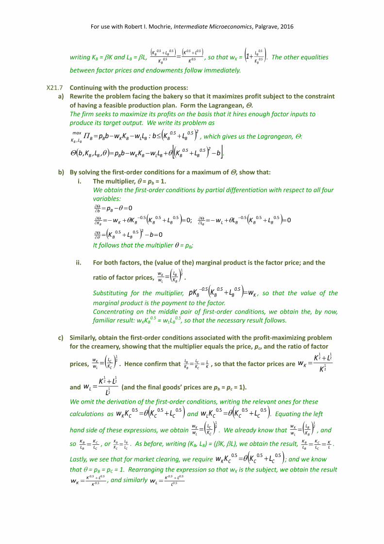
a) Rewrite the problem facing the bakery so that it maximizes profit subject to the constraint

of having a feasible production plan. Form the Lagrangean, . The firm seeks to maximize its profits on the basis that it hires enough factor inputs to produce its target output. We write its problem as

25.0B

5.0BBLBKBBL,K

max LKb:LwKwbpBB

, which gives us the Lagrangean, :

bLKLwKwbp,L,K,b25.0

B5.0

BBLBKBBB .

b) By solving the first-order conditions for a maximum of , show that:

i. The multiplier, = pb = 1. We obtain the first-order conditions by partial differentiation with respect to all four variables:

0

0;0

0

25.05.0

5.05.05.05.05.05.0

bLK

LKLwLKKw

p

BB

BBBLLBBBKK

Bb

BB

It follows that the multiplier = pB;

ii. For both factors, the (value of the) marginal product is the factor price; and the

ratio of factor prices, 21

B

B

L

K

KL

ww .

Substituting for the multiplier, K5.0

B5.0

B5.0

B wLKpK

, so that the value of the

marginal product is the payment to the factor. Concentrating on the middle pair of first-order conditions, we obtain the, by now, familiar result: wKKB

0.5 = wLLB0.5, so that the necessary result follows.

c) Similarly, obtain the first-order conditions associated with the profit-maximizing problem

for the creamery, showing that the multiplier equals the price, pc, and the ratio of factor

prices, 21

C

C

L

K

KL

ww . Hence confirm that K

LKL

KL

C

C

B

B , so that the factor prices are 21

21

21

K

LKwK

and 21

21

21

L

LKwL

(and the final goods’ prices are pb = pc = 1).

We omit the derivation of the first-order conditions, writing the relevant ones for these

calculations as 5.05.05.0CCCK LKKw and 5.05.05.0

CCCL LKKw . Equating the left

hand side of these expressions, we obtain 21

C

C

L

K

KL

ww . We already know that 2

1

B

B

L

K

K

L

w

w , and

so C

C

B

B

L

K

L

K , or

C

B

C

B

L

L

K

K . As before, writing (KB, LB) = (K, L), we obtain the result,

LK

L

K

L

K

C

C

B

B .

Lastly, we see that for market clearing, we require 5.05.05.0CCCK LKKw ; and we know

that = pB = pC = 1. Rearranging the expression so that wK is the subject, we obtain the result

5.0

5.05.0

K

LKKw

, and similarly

5.0

5.05.0

L

LKLw


X21.8 If the firms reach the allocation (KB, LB) = (K, L); (KC, LC) = (1 – )(K, L):

a) Show that MRTSB = 21

KL = MRTSC; and explain why this ensures that every allocation at

which the firms maximize profits is also Pareto-efficient.

We know from X21.7 that MRTSB =

5.0

B

B5.0

B5.0

B5.0

B

5.0B

5.0B

5.0B

Lb

Kb

K

L

LKL

LKK

B

B

; and that

MRTSC = 5.0

C

C

K

L

. It follows that if the bakery’s share of the endowment, (KB, LB) = (K, L),

so that the creamery’s share (KC, LC) = (1 -)(K, L), then the marginal rate of technical substitution is the same for both firms. We represent this property in an Edgeworth box by drawing isoquants that share a common tangent. This means that there is no possibility of either firm increasing its output without the other firm reducing its output, and so production is Pareto efficient.

b) Confirm that for both businesses, 21

21

21

K

LKKVMP

, and the marginal rate of transformation,

MRT = 1. Interpret this result. We define the value of the marginal product for each factor (for each firm) as the product of the output price and the marginal product of the factor: so for the bakery, the value of the marginal product of capital: VMPK

B = pBMPKB. We have already established that pB = pC = 1,

and the result follows.

The marginal rate of transformation MRT = 1c

b

p

p . As production of bread increases,

production of cheese has to be reduced by the same amount. (This is not a general result, but holds here because of our assumption of constant returns to scale in both production functions.)

c) In an Edgeworth box, sketch the Pareto set, and the isoquants passing through the allocation F: (KB, LB) = LK ,3

1 and (KC, LC) = LK ,32 .

In the Edgeworth box, we represent the endowment of capital by its length and the endowment of labour by its height. At division, F, the bakery’s use of capital is represented by the distance from the left edge of the box, and its use of labour by the height above the bottom edge. In this case, the Pareto set is the upward diagonal. We draw the division, F, so that it is one third of the distance from the bottom, left to the top, right corner of the box.

d) Show that at the allocation H: (KB, LB) = LK , and (KC, LC) = LK,1 , the bakery

produces b = 221

21

LK , while the creamery produces c = 221

21

1 LK

This result follows directly from the homogeneity property of the production function. Confirm that:

i. total output, b + c = 221

21

LK = y0;

This is simply the sum of the individual firm outputs in the case above. Note that with pB = pC = 1, the total firm revenue will also be y0.

ii. the value of output, pbb + pcc, equals the cost of production, wKK + wLL;

The cost of production C = wKK + wLL = LK 5.0

5.05.0

5.0

5.05.0

L

LK

K

LK = (K0.5 + L0.5)(K0.5 + L0.5)

= (K0.5 + L0.5)2 = y0.

iii. both firms make zero profits.


Since the revenues and costs are equal, this follows immediately.

e) Sketch the production possibility frontier, illustrating on it point J', corresponding to input allocation J. In a diagram with output of bread measured on the horizontal axis and output of cheese measured on the vertical axis, the production possibility frontier will, in this case, be a straight line, with equation b + c = y0, so that MRT = -1. At the intersection with the vertical axis, only cheese is produced; this is the equivalent of the bottom, left corner of the Pareto set in the Edgeworth box. Similarly, at the intersection with the horizontal axis, only bread is produced; this is the equivalent of the top, right corner of the Pareto set. For point J, a

proportion of the distance from the bottom left corner of the diagonal in the Edgeworth

box, point J1 will also be a proportion from the left hand edge of the production possibility frontier.

X21.9 Now consider the problem facing Richard and Seth.

a) Write down an expression for Seth’s utility, showing that he consumes the share of output (of both goods, and so of total output) that Richard does not. [Note: In other words, write

down an expression for Seth’s utility, given that bR + bS = b; cR + cS = c; and b + c = 221

21

LK

.]

It will be useful to remember that b = (K0.5 + L0.5)2 and that c= (1 - )(K0.5 + L0.5)2. Then Seth’s

consumption bundle, (bS, cS) = (b – bR, c – cR) = [(K0.5 + L0.5)2 – bR, (1 - )(K0.5 + L0.5)2 – cR].

Seth’s utility is US:

RR

25.05.0

S

25.05.0R

25.05.0

SS

SS

cbLK

bLK1.bLK

cb

cbSSS c,bU

.

b) Assume that Seth meets a utility target uS(bS, cS) = uS

0. Write down an expression for Richard’s utility maximization problem. Richard seeks to maximize utility subject to Seth’s utility target. We can write the problem as

0SSScb

cb

c,b

max uc,bU:RR

RR

RR

.

c) Calculate Richard’s marginal utilities, MUB

R and MUCR, and his marginal rate of substitution,

MRSR. Repeat the calculations for Seth.

For Richard, the marginal utility of bread, MUBR =

22

RR

R

RR

RR

RR

R

R

R

cb

c

cb

cb

cb

c

b

U

. In the same

way, we obtain marginal utility of cheese, MUCR =

22

RR

R

RR

RR

RR

R

R

R

cb

b

cb

cb

cb

b

c

U

. The marginal

rate of substitution, MRSR = 2R

RR

C

RB

bc

MU

MU . We omit the calculations but confirm that for

Seth, the marginal rate of substitution, MRSS = 22

R

R

S

S

S,C

S,B

bb

cc

b

c

MU

MU

.

d) Show that if the marginal rates of substitution are equal, then bc

bc

bc

S

S

R

R . Using the

argument developed previously, confirm that these conditions will be satisfied whenever

Richard consumes a proportion of the output of each good, and Seth a proportion (1 –

). [Note: This means that (bR, cR) = (b, c), and (bS, cS) = (1 – )(b, c).]

For the marginal rates of substitution to be equal, R

R

S

S

R

R

bb

cc

b

c

bc

. Cross multiplying and

expanding the brackets, bRc = cRb, and the result follows directly.


e) On the diagram showing the production possibility frontier, add an Edgeworth box which has its upper right-hand vertex at J'. Within the Edgeworth box, show the Pareto-efficient allocations that satisfy the conditions obtained in part (d). With b = c, we draw an Edgeworth box with the top right corner of the box at the midpoint of the production possibility frontier, so that the box represents the total outputs. We represent the bakery’s output by the length of the box and the creamery’s output by its height. At any division, H, within the box , Richard’s consumption of bread is represented by the distance from the left edge of the box, and consumption of cheese by the height above the bottom edge. The Pareto set will be the upward diagonal. We define two points on the Pareto set, H1, which is one quarter of the distance from the bottom, left to the top, right corner of the box; and H2, which is three quarters of the distance from the bottom, left to the top, right corner. In both cases, Richard’s and Seth’s indifference curves meet at their intersection with the Pareto set, and have a common tangent, which has gradient MRSR = MRSS = MRT = -1 (see below for calculations).

f) Calculate the common marginal rate of substitution for all allocations in the Pareto set.

Add indifference curves for Richard and Seth to your sketch, assuming that = ½, so that each consumes half of the output of both goods. Explain why the allocation of goods in the Edgeworth box is not consistent with a general equilibrium.

For Richard, MRSR = 222

bc

bc

b

c

MU

MU

R

R

R,C

R,B .

For Seth, MRSS = 22

1

12

bc

b

c

b

c

S

S

. The marginal rate of substitution is the same

for both, as required for Pareto efficiency. We note that we require the common marginal rates of substitution to be equal to the marginal rate of transformation.

g) Show that the condition MRSR = MRSS = MRT = c

b

pp

can only be satisfied when b = c =

221 2

121

LK . Sketch a new diagram showing the production possibility frontier; the

allocation H' for which b = c and the associated Edgeworth box; the Pareto set within the

box; the Walrasian equilibria when (i) = ¼ and (ii) = ¾; the indifference curves passing through the equilibria; and the common tangents to the indifference curves at each equilibrium. Demonstrate that the equilibrium conditions are indeed satisfied.

We have already shown that MRT = -1, so that MRSR = MRSS = 12

bc . We obtain the

result that b = c. We have already described the Edgeworth box in part e). The equilibrium conditions are all satisfied because on the Pareto set, the common marginal rate of substitution equals the marginal rate of transformation.

X21.10 Consider the situation in X21.9 where = ¾. Suppose that Richard agrees with Seth to a

reduction in the value of to ½. They then share the total factor incomes equally. a) Explain why we would not expect the product mix to change, so that the bakery and the

creamery would continue to hire the same quantity of factor inputs, and the combination of outputs in the economy would remain unchanged. We have demonstrated that Richard and Seth will always choose consumption bundles containing the same proportions of bread and cheese, so that with these (CES) preferences, market demands are independent of income shares.

b) Sketch a diagram showing: the production possibility frontier; the Edgeworth box and the Pareto set; the allocations of final goods before and after the change in income shares; and also the indifference curves passing through the Pareto-efficient allocations before and after the income change.


We have already seen that in a diagram with the quantity of bread measured on the horizontal axis, and the quantity of cheese measured on the vertical axis, that the production possibility frontier has the equation b + c = (K0.5 + L0.5)2, which is a straight line with gradient -1. We require that b = c = ½(K0.5 + L0.5)2, so that factors are allocated with production at the midpoint of the line. Then, given preferences, whatever the share of factor incomes accruing to Richard and Seth, they will both choose to buy equal quantities of bread and cheese, (so that bR = cR and bS = cS; and of course markets clear so that bR + bS = b and cR + cS = c. Making these choices, MRSR = MRSS = -1, so that their indifference curves through any Pareto-efficient division of goods share a common tangent, which lies parallel to the production possibility frontier. Before Richard transfers resources to Seth, the indifference curves meet three-quarters of the way up the diagonal of the Edgeworth box; afterwards, they meet at the midpoint of the diagonal (and indeed of the box).

X21.11 In X21.9, we obtained a linear production possibility frontier. Explain why we would

obtain a linear utility possibility frontier. Confirm that if factor inputs are not allocated so that b = c, then even if production is efficient, the utility profile will lie in the interior of the utility possibility set. The main argument for obtaining a linear utility possibility frontier is that the utility functions are homogeneous of degree 1. This means that if the division of goods is Pareto efficient, then increasing Richard’s utility by some amount will be accompanied by an equally large reduction in utility for Seth.

We note that if b c, then the Pareto set for the consumption problem will still be the diagonal of the Edgeworth box. However, if b < c, then the diagonal will be steeper and MRSR = MRSS < -1; so the common marginal rate of substitution is less than the marginal rate of transformation. By increasing production of bread (and reducing production of cheese), it is possible to effect a Pareto improvement.

X21.12 Working with the utility possibility frontier in X21.11, calculate the most-preferred utility

profile for the social welfare functions, w, where (a) w(uR, uS) = min(uR, uS); (b) w(uR, uS) = lnuR + lnuS; (c) w(uR, uS) = uR + 2uS; and (d) w(uR, uS) = uR

¾uS¼.

We write the linear utility possibility frontier, uR + uS = v0. Then uS = v0 – uR. a) If w(uR, uS) = min(uR, uS), then the social planner considers utilities to be perfect complements.

The planner’s objective is to maximize the lesser of uR and v0 – uR. So long as uR < v0 – uR, then increasing uR, min(uR, uS) = uR, and this expression increasesis increasing in uR. The same is true when min(uR, uS) = uS; increasing uS increases social welfare. As in previous examples, with this form of function, the welfare maximizing consumption profile (uR*, uS*) = (½v0, ½v0); and in terms of resources, the social planner directs transfers so that Richard and Seth share the factor income equally.

b) For this we simply require the usual first-order condition – that the marginal rate of substitution for the social planner is equal to the marginal rate of transformation – to be

satisfied. This occurs when MRT1MRSS

R

uw

uw

P

. Given the utility function. RR u

1uw

and SS u

1uw

. We therefore require uR = uS, or a division of resources that allows Richard and

Seth to generate the same utility. c) When w(uR, uS) = uR + 2uS, we have a planner who treats utilities as perfect substitutes;

however the planner also places greater weight on Seth’s utility than on Richard’s utility, and so we observe that MRSP = -0.5 > -1 = MRT. The planner gives all the resources to Seth.

d) Again, we require the usual first-order condition – that the marginal rate of substitution for the social planner is equal to the marginal rate of transformation – to be satisfied. This


occurs when MRT1MRSS

R

uw

uw

P

. Given the utility function, we obtain marginal

utilities in terms of partial derivatives 41

R

S

R u

u

43

uw

. Taking their ratio, we require uR = 3uS, or a

division of resources that allows in which Richard to derive three times the utility of Seth. X21.13 Using diagrams, explain why a social planner with a utility function such as (a) in X21.12

has a very strong commitment to egalitarianism. We are already familiar with the representation of preferences where goods are perfect complements. In a diagram with Richard’s utility, uR, measured on the horizontal axis and Seth’s utility, uS, measured on the vertical axis, we draw indifference curves as L-shaped, with the vertex of each indifference curve found on the line uR = uS. Drawing in a utility possibility

frontier, and placing the requirement that - < MRT < 0, so that the frontier is always downward sloping, then increasing Richard’s utility, Seth’s utility must decrease and there can only be one utility profile (uR*, uR*) where they both receive the same payoff. At this point, the first-order condition, that there is a common tangent to the utility possibility frontier and the social welfare function, is satisfied. Such a social planner will act to ensure that there is equality of outcomes.

X21.14 Suppose that the social planner’s preferences are captured by form (b) of the social

welfare function in X21.12. Sketch the social welfare indifference curves, w = 1, 2 and 3. What would you conclude about the slope of the utility possibility frontier on the line uR = uS if the planner chooses the utility profile (uR*, uS*): uR* > uS*? In a diagram with Richard’s utility, uR, measured on the horizontal axis and Seth’s utility, uS, measured on the vertical axis, we see that the indifference curves are rectangular

hyperbolae, with the equation uS = R

w

ue . These curves will be smooth, convex, downward

sloping, and will approach the axes, but never cross them.

For use with Robert I. Mochrie, Intermediate Microeconomics, Palgrave, 2016 Chapter 22 X22.1 Assume that the value of an hour’s leisure to a typical commuter is £15. If 20,000 cars

enter a city during the period of excess demand, calculate the daily and annual costs of a 30-minute delay every day. What do you conclude about the size of the investment needed to eliminate congestion? We estimate the value of foregone leisure (per day) to be 15*0.5*20,000 = £150,000. We estimate the value of removing congestion from the city during the rush-hour (250 days per year, with a 10-year payback period) to be of the order of £375m. Given that, this is the value of a relatively modest public infrastructure project (the construction cost of the Øresund Bridge, linking Copenhagen and Malmö, was approximately DKK30bn, or about £3bn, when it opened in 2000.)

X22.2 In the short-run analysis of production, we argue that the marginal product of labour will

be eventually diminishing, and this ensures that firms will not expand its use without limit. Explain why, given our present assumptions, we might expect the farmer to be happy always to have more beehives on the land. Criticize the argument. [Hint: Think of the problem of commuting.] We have made the assumption that the marginal product of labour will always be positive. There is no cost to having beehives on the farm in the current specification of the model, but this is not possible – apart from anything else, there is a risk of congestion, and presumably also at very high densities, there would be concerns about safety.

X22.3 Show that there is a positive externality on production of honey from choice of orchard

size, T. Explain how this affects the choice of labour input, Lb, and the quantity of honey

produced. Confirm that so long as we assume T

MPbL

> 0, the beekeeper would always

prefer a larger to a smaller orchard.

In Expression 22.6, differentiating the marginal product of labour, bLb

, with respect to

orchard size, T, we obtain bLb

T

> 0, by assumption. Increasing T, the marginal product

increases; equilibrium is reached with a larger labour input, and the beekeeper benefits from the orchard increasing in size.

X22.4 Consider the following situation. We write the short-term production function for the

farmer, A: A(Lf, b) = 50Lf0.5b0.25; the short-term production function for the beekeeper, b:

b(Lb) = 4Lb0.5; and the associated output of honey, h: h(b) = 125b. The price of apples, pa =

2, while the price of honey ph = 8. The farmer’s wage, wf = 10, and the beekeeper’s wage, wb = 20.

a) Write down the farmer’s profit function. Partially differentiate the derivative with respect to the labour input, Lf, and, by obtaining the first-order condition, show that the farmer maximizes profits by working Lf

P = 25b½.

We obtain the profit f: f = paA - wfLf = 2[50Lf0.5b0.25] – 10Lf. Differentiating,

010bL50 25.05.0fL f

f

if Lf0.5 = 5b0.25; and squaring both sides, we obtain the required

expression for the profit maximizing use of labour.

b) Write down the beekeeper’s profit function. Partially differentiate the derivative with respect to the labour input, Lb, and, by obtaining the first-order condition, show that the beekeeper maximizes profits by working Lb

P = 10,000.


We obtain the profit b: b = ph.h(b(Lb)) – wbLb = 8.125.[4Lb0.5] – 20Lb. Differentiating,

020L000,2 5.0bLb

b

if Lb0.5 = 100; and squaring both sides, we obtain the result.

c) Calculate the size of the beehives, the total outputs of apples and honey, and the total

revenues, costs and profits of both the farmer and the beekeeper. We have found the following: Lb= 10,000; b = 4Lb

0.5 = 400; Lf = 25b0.5 = 500; output of apples Af = 50Lf

0.5b0.25 = 250b0.5 = 5,000; output of honey, h = 125b = 50,000. Revenue from sale of apples Rf = 2A = 10,000. Cost of production, Cf = 10Lf = 5,000, so profit

for farmer f = 5,000. Revenue from sale of honey, Rb = 8h = 400,000. Cost of production Cb = 20Lb = 200,000, so

profit for beekeeper b = 200,000. X22.5 Continue with the situation set out in X22.4.

a) Write down the social planner’s payoff function as the sum of the farmer’s and the beekeeper’s profit functions. Partially differentiate the function with respect to the labour inputs, Lf and Lb. Confirm that the optimal labour input for the farmer Lf

S = 25b0.5, and that the socially optimal labour input for the beekeeper reflects both the optimal private use plus the positive externality on the farmer’s production.

We write the social planner’s objective, S: S = 2(50Lf0.5b0.25) + 8(500Lb

0.5) – 10Lf – 20Lb.

Note that b = 4Lb0.5. Partially differentiating with respect to Lf, 010bL50 25.05.0

fL f

S

,

if Lf0.5 = 5b0.25; and squaring both sides of the expression, the result follows.

Partially differentiating the payoff, S, with respect to Lb, we obtain

20L000,2L2.bL50 5.0b

5.0b

75.05.0f2

1Lb

S

. The first term in this partial derivative is the

effect of the externality.

b) Without attempting calculations, compare the socially optimal and the privately optimal sizes of beehives. Discuss the impact of beehive size on the total outputs of apples and honey, and the total revenues, costs and profits of both the farmer and the beekeeper. The optimal size of the beehive increases because we take account of the indirect effect of the beehives on apple production and profits. With a larger beehive, the farmer produces more apples, and the beekeeper more honey.

X22.6 Discuss how the farmer might be able to encourage the beekeeper to increase the level of

output from the privately optimal to the socially optimal level. Given the circumstances, we would expect the farmer not simply to allow the beekeeper to place hives in the orchard, but to pay the beekeeper for providing the pollination service.

X22.7 Adapt Expressions 22.2 and 22.5, so that the farmer subsidizes the beekeeper’s wage at a

rate, sb. Find the new first-order condition, and the value of the subsidy, sb, that will lead to the socially optimal outcome.

The farmer’s profit can now be written as f: f = pAA(Lf, b, T0) – wfLf – sbLb – rT0. The

beekeeper’s profit can be written as b: b = phh[b(Lb, T0)] - (wb - sb)Lb. As before, the farmer’s profits are determined by both of the labour inputs, but through making a payment to the beekeeper the farmer is able to affect the beekeeper’s choice of labour input. We obtain first-order conditions, by partially differentiating profits with respect to their own

labour input for both the farmer and the beekeeper: 0wp fLA

AL ff

f

; and

0swp bbLb

bh

hL bb

b

. Comparing this expression with expressions obtained in X22.5,


we conclude that if the farmer is able to pay the subsidy equal to the marginal benefit of the externality, then the beekeeper will choose the socially optimal level of the externality.

X22.8 Sketch a diagram showing the situation facing a firm and the market in long-run

equilibrium where there is perfect competition with the long-run supply curve: (a) perfectly flat; and (2) downward-sloping. Show how a change in demand conditions affects the equilibrium in each case. The analysis of firm and industry behaviour was presented in Chapter 14. We draw the diagrams with two panels, the left-hand one illustrating firm decision making and the right-hand one illustrating the market outcomes. Both panels have measures of revenue and cost shown on the vertical axis, with firm output measured on the horizontal axis of the left panel and market output on the horizontal axis of the right panel. Beginning with the long-run supply curve being flat, we illustrate this in the right-hand panel by a flat line, p = p0. In the left panel, we also draw in the line MR(qf) = AR(qf) = p0, showing that the firm’s demand is perfectly elastic at this market price. In the left-hand panel, we also draw in a U shaped average cost curve, which has its minimum at some output q0 where the flat line, MR(qf) = p, is tangent to the average cost curve. Then, drawing in a marginal cost curve which intersects the average cost curve at its minimum, we see that the profit maximizing condition MC = MR is satisfied when q = q0, and since AC(q0) = AR(q0), the firm makes zero profits. We argued in Chapter 14 that the expansion of the market will be achieved through entry, with firms remaining at the same scale as demand increases. We illustrate this in the right-hand panel by sketching two curves representing market demand, noting that the market price given by the intersection of market supply and market demand does not change with demand conditions, so that profit maximizing firms maintain their output. We largely replicate the analysis in the second diagram. Now, though as market demand increases, the market price falls from p0 to p1. For the firm, this means that MR = AR = p1 after the increase in demand. We have seen that ACmin = p0 with constant returns to scale. With increasing returns to scale, we require the firms in the market to use resources more efficiently as the market size increases, so that the marginal cost curve for the firm in the left hand changes, lying below the original marginal cost curve at all levelof output. It follows that there will also be a new average cost curve, and we require that average cost curve to have its minimum at some output q1 >q0, where, similarly to before, AC(q1) = AR(q1) and MC(q1) = MR(q1), so that profit-maximizing firms make zero profits.

X22.9 One important element of cooperation in an industrial district is the emergence of

technical colleges, often funded with endowments by local businesses. Discuss their role in enabling businesses to increase productivity. Colleges enable workers to increase their skills, and through such training to increase their productivity. The output of the firms hiring them will also increase. Yet since workers are mobile, there is a positive externality associated with training workers within a firm, and so collaboration can increase the level of training beyond the level associated with the private solution.

X22.10 Confirm that for f > 0, average costs AC1(f) > AC0(f), and marginal costs MC1(f) > MC0(f).

This is quite straightforward, since h is increasing in C0 and h > 1. We write C1(f) = h[C0(f)].

Then the average cost, AC1(f) = f

fC

f

fC 01 = AC0(f); and the marginal cost MC1(f) =

fMC0dCdh

0 > MC0(f).

For use with Robert I. Mochrie, Intermediate Microeconomics, Palgrave, 2016 X22.11 To what extent is it reasonable to expect the owners of the power station to compensate

the owners of the fish farm for the loss of profits that might occur as a result of the power station opening? Your answer to this question is likely to depend upon the characterization of the problem that you choose. If you consider that the fish farm has had access to clean water before the power station was built, and that in effect it has a right to expect clean water, then it should be able to demonstrate that the operation of the power station is detrimental to its activities, and to that extent, it deserves compensation. Alternatively, if you consider that it is simply accidental that the fish farm has had clean water, and that it has simply used the river water because that is most convenient for it, then, while accepting that the operation of the power station is detrimental to the fish farm’s activities, you might argue that if the fish farm wishes for cleaner water, then it should pay the power station to reduce its pollution. Your answer should therefore turn on the question of whether the fish farm has a right to clean water, or whether the power station has an unrestricted right to use the water from the river.

X22.12 Define the social costs of power production as the sum of the direct costs, measured by

the power station’s cost function, C(w), where w is its output, and the costs experienced by other businesses, S(w), which are directly attributable to pollution resulting from power generation. Assume that the power station has entered into long-term wholesale contracts, and so can sell any quantity of power at a constant price, pw. Explain how the power station’s optimal output would differ were the power station required to provide compensation for the loss suffered by other businesses. In the private solution, the power station only considers its direct costs, C(w). We expect it to

adopt the efficient production level, w0, chosen so that MC(w0) = dwdC

= p(w0). In a socially

efficient solution, the power station considers both private and social costs, and so we define the social cost, SC: SC(w) = C(w) + S(w). Then the efficient solution will occur at production

level w1, chosen so that MSC(w1) = dwdS

dwdC = p(w1).

X22.13 Confirm that where the private solution is allowed to emerge, the power station makes

(economic) profits, but when the social optimum is imposed, it makes losses. We draw the diagram so that output is measured on the horizontal axis and value measures are shown on the vertical axis. We show the market clearing price as a flat line, on which for any level of output, E, MR(E) = AR(E) = p. We show the marginal (private) cost as a U-shaped curve, which starts from the vertical axis above p, cuts through the line MR = p, reaches a minimum, and then increases intersecting the line MR(E) = p when E = E0*. This is the firm’s profit maximizing output. For the firm to make profits, consider the two areas enclosed by the marginal revenue curve and the marginal cost curve to the left of E = E0*. The area below the marginal revenue curve must be larger than the one above the marginal revenue curve (remember that when marginal cost is greater than marginal revenue, then increasing production reduces profits). For the case of social costs, we draw the marginal social cost curve so that it is also U shaped, but lying above the marginal private cost curve. As drawn in Figure 22.3, where marginal social cost is always greater than marginal revenue, the firm fails to make social profits. More generally, we draw it so that it intersects the marginal revenue curve (twice), with the profit maximizing output at E1*, where marginal cost is increasing. The firm makes (social) losses if the area enclosed by the marginal cost and marginal revenue curves below the marginal revenue curve is less than the area enclosed by the curves above the marginal revenue curve.

For use with Robert I. Mochrie, Intermediate Microeconomics, Palgrave, 2016 X22.14 We have argued that power networks are likely to experience increasing returns to scale in

production. Adapting Figure 22.3, explain why this might increase the need to impose the socially optimal outcome. We draw the diagram so that output is measured on the horizontal axis and value measures are shown on the horizontal axis. We continue to draw the marginal revenue and average revenue curves as being the same flat line, so that for any level of output, E, MR(E) = AR(E) = p. With increasing returns to scale, the marginal cost curve is always downward sloping. Once it is below the marginal revenue curve, it remains below it for all higher levels of output. This implies that the first-order condition for profit maximization can never be met (and this is the basis for the argument that there would be a natural monopoly in this market). We can, though, create a marginal social cost curve that is eventually increasing, and argue that the welfare maximizing level of output will be achieved where this intersects the marginal revenue curve from below, at output E1*.

X22.15 We have assumed in this argument that there is no change in the market price, assuming that the power station faces perfect competition. Consider the situation facing the industry, and explain why this is unlikely. Indicate what you would expect to happen to the market price and the quantity produced, taking into account the likely effects on the market price and the quantity that each firm will produce. Power generation has typically used technologies in which there are very substantial scale economies, so that efficient power stations require substantial capital. This means that across a large range of possible outputs, power generation businesses will experience diminishing marginal costs, and they can expect to have substantial market power. We therefore expect these firms’ marginal revenue functions to be decreasing in output, so that when maximizing profit, they set price above marginal cost, and restrict output.

X22.16 Compare the marginal tax rate imposed when applying the Pigovian and the flat-rate tax.

The marginal tax rate under the Pigovian tax rate is the difference between the marginal social cost and the marginal (private) cost at every level of output, and so both average and marginal tax rates vary as the marginal rates change. The flat-rate tax will be set so that it has the same effect as the Pigovian tax. It is set so that the quantity traded Q(t)clears the market at price (including tax), so that the marginal social cost, MSC(Q(t)) = MSB(Q(t)), the marginal social benefit. Note that where the Pigovian tax changes as market conditions change, the flat-rate tax will need to be adjusted consciously by the government.

X22.17 Repeat the analysis of the imposition of a tax, assuming that the government applies an ad

valorem tax (that is, a tax that is a constant proportion of the value of sales). Explain why the Pigovian tax will be an ad valorem tax when both the marginal private cost and the marginal social cost functions are linear. Our analysis is essentially the same as above. The ad valorem tax is proportional to the price set, and so may need to be adjusted as market conditions change. In the case where marginal private cost and marginal social cost are both linear in output though, their difference, the marginal tax rate, will also be linear.

X22.18 Treating the government as a social planner, what concerns might it have about the effect

of a tax on a single good in general equilibrium? [Hint: Think of the condition that MRT = MRS for all goods.] The marginal rate of transformation (MRT) is represented for any output combination on the production possibility frontier as the gradient of the tangent to that point on the frontier. In a competitive equilibrium, MRT equals the ratio of the prices received by producers. The


marginal rate of substitution is the rate at which individual consumers substitute one good for the other, maintaining constant utility. In a competitive equilibrium, MRS equals the ratio

of the prices paid by consumers. If a tax changes one price only, then MRT MRS. X22.19 Adapt Figure 22.5 to show the situation in which the combination of licence and fine fails

to reduce the externality to the optimal level. The diagram is exactly the same except that at the level of output where the fine starts to be imposed, the marginal (private) cost + fine will be less than the market price. The curve labelled MCP + f therefore begins below the flat line, labelled Price, and intersects it to the right of output E1*. This intersection will be the output, with firms willing to pay the fine, and produce an output in excess of the maximum permitted level.

X22.20 Suppose that the government is able to require producers to pay a licence fee, without

which all production is illegal. Indicate on your diagram the size of the largest fee that the government could persuade a power station to pay. The largest amount will be the area bounded by the marginal private cost curve and the line labelled ‘Price,’ which is effectively the marginal revenue curve. This is the producers’ surplus. Restricting output to E1*, the producers’ surplus would be the area between the marginal private cost and marginal revenue curves, but to the left of the line E = E1*.

X22.21 Confirm that whether or not a licence fee is collected, the usual efficiency conditions for

general equilibrium cannot be satisfied when production is restricted. [Hint: Concentrate on the values of the marginal products of input factors, assuming that businesses require both capital and labour inputs.] Factors of production tend to be more productive – that is, have a higher marginal product – when the scale of production is restricted. So the value of the marginal product of factors in industries where there is a production quota is likely to be higher, so that the factor and output prices will be higher than where there are no restrictions. We conclude that there will be inefficiencies in the resource allocation. The requirement for efficiency, that the marginal rate of transformation is equal both to the ratio of factor prices and to individual consumers’ marginal rate of substitution, is no longer satisfied.

X22.22 Suppose that the government issues licences allowing firms to produce any output up to

the socially optimal output E1*, but with a fixed payment, irrespective of the scale of output. Assume that the government sets the fee so that it captures the entire surplus of a business operating at the maximum scale. Show that no business will wish to enter the market and operate at a smaller scale. Discuss why the businesses already in the market might be willing to accept such a restriction. This is a different proposal from a per-unit, or ad valorem tax. It is intended to be a lump sum tax, very similar to the proposal for licensing. The amount of the lump-sum tax is the maximum producer surplus. Firms that do not produce at the level of output allowing them to generate this will make losses; existing firms will make no profits, but will still be economically viable.

X22.23 We continue to assume that the activities of a power station include pollution of the water

supply for all firms operating downstream. Instead of licensing power generation, the government tolerates the production of the externality, here pollution. (It is still possible to detect all unlicensed emissions costlessly; and the fines imposed for failure to obtain licences in advance are large enough to ensure perfect compliance.) We also assume that the licensing environment involves two elements. Power stations can either:


undertake to pay the costs of pollution recovery directly, c = c1x + c2x2, where x is

the level of pollution; or else

purchase a licence permitting the production of a specific number of units of pollution, paying a fee f per unit.

All power stations generate pollution x = x1E, where E is the plant’s power output. a) Write down an expression for the costs of: (i) recovering the externality; and (ii) paying the

licence fee in terms of the output of power.

The total abatement cost, C = c1x + c2x2; the marginal abatement MAC = xc2c 21dx

dC . In

terms of the power output, since x = x1E, where E is the power output, MAC = 1x

E21 c2c . The

marginal fee, dxdF

= f1.

b) Calculate the level of output, x*, above which a power station would prefer to pay the

fixed licence fee rather than the recovery costs.

The firm will choose to pay the fee when c1 + 2c2x > f1, or when x > x* = 11c21 cf

2 .

c) Show that if process innovation leads to a reduction in the value of c2, the value of x* will

also increase.

Formally, we differentiate and confirm that 02c*x

. Intuitively, we note simply that the form

of the expression for x* indicates that x* is inversely related to c2, so that any reduction in c2 leads to an increase in x*; and firms will tend to switch from paying the licence fee to paying the recovery costs.

X22.24 We typically define the marginal abatement cost for a power station as being the rate of

change in the cost of reducing production of an externality with the level of output. Assume that a power station is initially producing externality x0, but recovers a quantity, x, and that its total abatement cost, c = c1x + c2x

2. a) Write down an expression for the marginal abatement cost.

The marginal abatement cost is as defined in X22.23: MAC(x) = c1 + 2c2x.

b) Sketch a diagram showing the marginal abatement cost (but show the unrecovered component of the externality on the horizontal axis, so that the curve is downward-sloping). Assume that the government charges a fee f for each unit of the externality that is not recovered. Show the power company’s preferred level of recovery. In a diagram, showing the unrecovered quantity of pollution on the horizontal axis and costs on the vertical axis, the graph of the marginal abatement cost is a downward-sloping line segment with gradient -2c2. It passes through the vertical axis at (0, c1 + 2c2x0), and extends as far as (x0, c1). Showing the government imposed cost, f, charged on non-recovered pollution, the firm will pay the fee on the quantity (x0 – x*), defining x*: c1 + 2c2x* = f, as in X22.23.

c) Suppose that improvements in the recovery technology lead to a reduction in the value of c2. Confirm that the power station will choose to increase the extent of recovery. This is perhaps done most easily on a graph. The effect of the reduction in the marginal abatement cost is seen as an anti-clockwise rotation of the MAC curve around (x0, c1). This has the effect of shifting the intersection of the MAC curve and the line c = f to the left, so that x*, the quantity recovered by the firm, increases.


d) Similarly, suppose that improvements in the production technology lead to a reduction in the value of x1 at any level of output. Confirm that the power station will treat this as an improvement in technology that reduces its marginal cost, and will therefore tend to increase its output, while reducing production of the externality. For the firm, taking into account the charging regime, profits depend upon output and the

extent of pollution, so = (E, x). But we have defined pollution, x: x = x1E, a linear function of output, E. A reduction in the value of x1 would mean a reduction in the level of pollution for any level of output, and would reduce the costs imposed on the business. The firm therefore increases its output, while reducing pollution.

e) For marginal social cost MCS = s1 + 2s2x, calculate the output at which the marginal recovery cost and the marginal social cost are equal. Explain why this is likely to be an economically efficient outcome. Marginal social cost increases in the level of unrecovered pollution. When marginal social cost equals marginal abatement cost, the benefit to society of further recovery is less than the cost of the activity; the first- (and second-) order conditions for an optimum are satisfied.

With MCS = s1 + 2s2x and MAC = c1 + 2c2(x – x0), equating these expressions, x = 22

0211

22sc

xccs

.

For use with Robert I. Mochrie, Intermediate Microeconomics, Palgrave, 2016 Chapter 23 X23.1 Discuss the extent to which the following are likely to be either non-excludable or non-

rivalrous in consumption: a) Air (that is, the gases constituting the atmosphere of the earth).

This is neither excludable nor rivalrous: we all breathe (from birth), and in doing so do not exhaust the atmosphere.

b) Water held in a reservoir for domestic and industrial usage. Excludable and rivalrous: without a connection to the distribution system, access is impossible (although it may be quite difficult to remove access once granted); and as widespread droughts (e.g. in the South West of the USA) demonstrate, use by one group reduces the ability of others to consume.

c) The road system surrounding a city; and the pavements of the city streets. Non-excludable, but rivalrous: there is no charge for entry; and the discussion of congestion in Chapter 22 confirms rivalry.

d) The public transport system (rail, buses, trams, etc.). Excludable (in principle) and rivalrous: while on many systems, it is possible to board vehicles without paying for a ticket, such behaviour is generally illegal. Again, the resource becomes congested during periods of peak demand.

e) The benefits of an inoculation campaign for an infectious disease such as polio. Non-excludable and non-rivalrous: Costs will be borne from public funds, and there is generally a positive externality, in that sufficiently high levels of inoculation will reduce the probability of infection to close to zero – in the case of polio, potentially globally.

f) The national defence and security services provided by the government. Non-rivalrous and non-excludable: there have been legal challenges brought by pacifists to the collection of taxes that might be used to fund defence expenditure; none has been successful. All benefit from these services, and the benefit is enjoyed without private use of the resource.

g) Global positioning by satellite technology. Non-rivalrous and non-excludable: formally part of the national defence service of the United States of America, it can be used without restriction anywhere on the surface of the earth (see below for further discussion).

X23.2 What evidence is there that people’s WTP for the location identification services provided

by GPS is greater than zero? People are willing to buy and rent devices that provide no other services; although these are being subsumed by somewhat simpler services provided by smartphone.

X23.3 GPS was developed by the Department of Defense in the USA for its own purposes. Why

might we expect a government agency to have taken the lead in this project, rather than relying on market-based institutions to provide the investment? We might reasonably ask who, other than government, would wish to develop such a service. In order for private provision to develop, there has to be a market for the service. Note that smartphones often do not use GPS to provide mapping services, but rather rely on the


terrestrial network of local transmitters, so that such mapping services are bundled with their other services.

X23.4 Consider a proposal to install streetlights in a small village. The proposal will go ahead if

the amount that each villager is willing to contribute to the fund meets the cost of providing the lights. What difficulties might there be in relying only on voluntary contributions to fund the scheme? Anyone living in the village who does not provide any contribution cannot easily be denied access to the service, which is neither rivalrous nor excludable.

X23.5 Confirm that if the sum of household valuations, V: PcVn

hh

1

, then the proposal to

install streetlights must fail.

When PvVn

1hh

, then the total value of the service to the households is less than the price

of providing it. The sum of contributions, C V; otherwise, there are people offering to pay more than their WTP.

X23.6 Assume that vh = v, so that every household places the same value on the service, and that

the feasibility condition in X23.5 is satisfied. Confirm that there are two symmetric Nash equilibria: (a) where ch = 0 for every household; and (b) where ch = c, and C = nc = P. Discuss whether equilibrium (a) or equilibrium (b) seems more likely to occur. We assume that all except one household has made its decision, with the other (n -1) having adopted the Nash equilibrium strategy.

a) With n – 1 household having decided to make contribution ch = 0, household n can make contribution cn: 0 < cn < v, and be worse off than when making contribution cn = 0; the contribution is not sufficient on its own to provide the service, and the individual will not meet the whole cost of provision. So cn = 0 is a best reply, and strategy ch = 0 supports a symmetric Nash equilibrium.

b) With n – 1 household having decided to make contribution ch = c = nP

, household n can make

contribution cn = c, ensuring that supply is (just) fully funded. Offering more would not increase access to the good, and so the household would be worse off offering cn > c than when making contribution cn = c; and contribution cn < c would not be large enough to secure the service. So cn = c is a best reply, and strategy ch = c supports a symmetric Nash equilibrium. We might consider that the equilibrium in a) will emerge if there is a low trust situation, while the equilibrium in b) might emerge in a higher trust situation; we would analyse these outcomes in terms similar to the Stag Hunt game, using mixed strategies in which the expected payoff to contributing would equal (or exceed) the expected payoff to not contributing.

X23.7 Confirm that there is an equilibrium in which for household n, cn = 0, but for all other

households, 1

nP

hc < v. Discuss the likelihood of being able to sustain such an

equilibrium. We do this in two parts. Firstly, we note that for household n, given the strategy of the other n – 1 households, the level of provision will not increase for any value of ch = 0, so that cn = 0 is the best reply to the other households’ strategy. Secondly, we note that for all of the other n – 1 households, any contribution less than ch leads to the failure of supply; the household cannot be better off. For contributions c > ch, the level of provision does not increase, so


again, the household cannot be better off. The proposed action profile is therefore a set of consistent best replies, and so a Nash equilibrium.

X23.8 Suppose that Vishal and William live in houses at the end of a narrow track, 100m in

length. They have received an offer from a local contractor who is willing to pave and widen the track as part of a development project, but Vishal and William have to meet the cost of provision, which is £250 per metre. Assume that Vishal’s marginal willingness to pay, MWTPV = £125/m; while for William, MWTPW = 250 – 1.25x, where x is the length of paved road.

a) Sketch a diagram to show the marginal cost, the individual MWTP curves, and the market MWTP curve. Indicate the economically efficient outcome, and confirm that this involves paving the full length of the track. On a diagram with the length of paved road, x, shown on the horizontal axis and measures of cost and benefit on the vertical axis, we show the marginal cost as the horizontal line, MC = 250. Similarly, we show Vishal’s MWTP as the flat line MWTPV = 125. William’s MWTPW is a downward sloping line segment, connecting (0, 250) on the vertical axis with (100, 125); while the market MWTP, MWTPM = MWTPV + MWTPW. This will be a line, parallel to William’s MWTPW curve, but connecting (0, 375) with (100, 250). Given that MWTPM(100) > MC(100), the track will be built.

b) Suppose that the marginal cost of provision were to increase to £300/m. How would you expect the efficient outcome to change? With the increase in marginal cost, the standard first-order condition will apply, and the track will run where MWTPM > MC, or where 375 – 1.25x > 300, or where x < 60. The contractor leaves 40m of track unpaved.

c) Suppose instead that Vishal’s circumstances change and he has to use the track more often. Now MWTPV = 250. If William knows this, how might his behaviour change? William knows that MWTPV = MC. So he realizes that Vishal will be willing to pay for the track to be paved. He may refuse to make any contribution, and still be able to use it.

X23.9 Given the problem in Expression 23.5:

a) Form the Lagrangean, and by partial differentiation with respect to R, SV and SW, obtain the first-order conditions (FOCs), which must be satisfied in a Pareto-efficient outcome. [Hint: Note that there will be two Lagrangean multipliers.]

We write the Lagrangean (R, SV, SW, , ) = UV(R, SV) + [UW(R, SW) - U0] + (m – pR - SV – SW). We obtain five first-order conditions, by partial differentiation with respect to each of the variables:

0pR

U

R

U

RWV

; 0V

V

V S

U

S

; 0W

W

W S

U

S

; UW(R, SW) - U0 = 0;

and m – pR - SV – SW = 0.

b) By expressing the multipliers in terms of the partial derivatives, confirm that for any Pareto-efficient allocation, (R*, SV*, SW*):

p

W

W

W

V

V

V

S

UR

U

S

UR

U

[23.6]

Given that pR

U

R

U WV

; we can substitute for , since

V

V

S

U

. Then

W

W

V

V

W

W

S

US

U

S

U

; and on substituting for and , and rearranging, the required result follows.

For use with Robert I. Mochrie, Intermediate Microeconomics, Palgrave, 2016 X23.10 Given quasi-linear preferences, as in Expression 23.7:

a) Write down expressions for the marginal utilities and the marginal rate of substitution for both Vishal and William. From Expression [23.7], partially differentiating UV, we obtain marginal utilities

MUR,V = R

uV

, and MUS,V =

S

uV

= 1. Similarly, partially differentiating UW, we obtain marginal

utilities MUR,W = R

uW

, and MUS,W =

S

uW

= 1.

The marginal rates of substitution are then (minus one times) the ratio of marginal utilities,

so that MRSV = R

u

S

uR

uV

V

V

V

. In the same way, MRSW = R

u

S

uR

uW

W

W

W

.

b) Confirm that the marginal rate of substitution depends only on the level of provision of the

public good. Since the marginal utility of the private good is constant, the level of its consumption does not enter into the marginal rate of substitution.

X23.11 Suppose that there is only Vishal’s house at the end of the track, and that his utility

function, UV = R. We now write his problem, VVVSRmSpRSR

V

:,

max .

a) Confirm that the marginal rate of substitution, MRSV = 1R

. Hence sketch the

indifference curves UV = 1, 2 and 3. Confirm that when R = 1, MRS = –1 on all three indifference curves.

From X23.10, we see that MRSV = R

uV

. Applying the formula to the expression for Vishal’s

utility, the result follows. On a diagram with consumption of the public good on the horizontal axis and consumption of

the private good on the vertical axis, the indifference curve, R + SV = 1; or SV = 1 – Ra, begins from the vertical axis at (0, 1), where the curve is vertical. It is downward sloping and convex, and meets the horizontal axis at (1, 0), where it has gradient -1. The indifference

curve R + SV = 2; or SV = 2 – Ra, begins from the vertical axis at (0, 2), where the curve is

vertical. It is downward sloping and convex, and meets the horizontal axis at 0,2 a1

. Lastly,

the indifference curve,

R + SV = 3; or SV = 3 – Ra, begins from the vertical axis at (0, 3), where the curve is vertical. It

is downward sloping and convex, and meets the horizontal axis at 0,3 a1

.

b) Show that if p = = 0.5, and if mV > 0.5, Vishal’s most-preferred, affordable consumption bundle, (R*, S*) = (1, mV – 0.5). On your diagram, sketch Vishal’s income expansion path.

We write Vishal’s problem as VVV5.0

S,R

max mSR5.0:SRV

. Then the condition

MRSV = 5.0R2

1 = ½ is satisfied when R = 1. The income expansion path begins from the origin,

runs along the horizontal axis, until R = 1, and is then the segment of that vertical line above the axis.

X23.12 We return to the situation where Vishal and William share the access road, writing

William’s utility function, UW = R + SW.

a) On a diagram, sketch both Vishal’s and William’s marginal rate of substitution as the value of R increases.


We know that the marginal rates of substitution MRSV = MRSW = 1R

. The marginal rate of

substitution increases as R increases; for R 0, MRS -; while as R , MRS 0

b) Confirm that both for Vishal and for William, the marginal rate of substitution does not vary with the house sizes, SV and SW. We have already confirmed this.

c) Apply and interpret the condition in Expression 23.6 in this case. Since the marginal utility of consumption of the private goods is constant (and scaled to 1),

we obtain p = R

U

R

U VV

=

1R

2 . The price of supply for the public good is set so that it is the

sum of consumers’ marginal utilities. X23.13 Anya, Brinda and Claudia want to find the socially preferred outcome.

a) Suppose that they each have one vote, which they may cast for their own most-preferred outcome. What will happen? Each votes for their most-preferred outcome, and there is a tie.

b) Suppose that they agree to engage in successive comparisons of pairs of outcomes. Show (i) that if x is compared with y, and then the more-preferred outcome is compared with z, they will choose z; but (ii) that if y is compared with z, and then the more-preferred outcome is compared with x, then x will be preferred. In case (i), comparing x and y, x obtains 2 votes, while y obtains 1 vote. Then comparing z and x, z obtains 2 votes and x obtains 1. So z is chosen. In case (ii), comparing y and z, y obtains 2 votes, while z obtains 1 vote. Then comparing x and y, x obtains 2 votes and y obtains 1. So x is chosen.

c) Show that it is possible using successive pairwise comparisons for y to be most preferred. Suppose we first compare x and z. Then z obtains 2 votes, and x obtains 1 vote. We compare y and z; and y obtains 2 votes, while z obtains 1. So y is chosen.

X23.14 Claudia decides that this situation is too complicated and leaves. Anya and Brinda now try

again, with each assigning three points to their most-preferred, two to their second-ranked, and one to their least-preferred, outcomes.

a) Confirm that on this basis they will choose outcome y. Anya scores the outcomes: x = 3, y = 2, z = 1, while Brinda ranks them y = 3, z = 2, and x = 1. Adding together the scores, we obtain y = 5, x = 4 and z = 3, so they choose y.

b) Suppose instead that, before evaluating their preferences, they agree that since neither of them ranks outcome z highest, they should exclude it. How would this affect their choice? Anya scores the outcomes: x = 2, y = 1, z = 0, while Brinda ranks them y = 2, x = 1, and z = 0. Adding together the scores, we obtain x = y = 3, so that they are undecided.

X23.15 Suppose that vX = 1,000. Confirm that Xavier is still pivotal, and that the social planner will

still require him to make a transfer, kX = 200. We have vv = vW = 500, so that subtracting their contributions, each obtains a surplus of -100. The planner will only proceed with the project if vX > 800, so that Xavier obtains a surplus of greater than 200. By requiring a transfer of 200, Xavier gives up an amount equal to the loss that the others suffer.

For use with Robert I. Mochrie, Intermediate Microeconomics, Palgrave, 2016 X23.16 Consider a case in which we have a public good for which total cost, C = 5,000, and with

five possible participants, i = 1, … , 5, benefiting from provision, with values v1 = 1,500, v2 = 1,200, v3 = 1,000, v4 = 700, and v5 still to be declared. The social planner announces that the project requires initial contributions, ci = 1,000. Show that:

a) For 300 v5 < 600, completion is inefficient; and participants 4 and 5 are pivotal, and so should transfer k4 + k5 = 700. Completion is inefficient. The loss to participants 1 and 2 is still 700, and so the planner seeks transfers totalling that amount from participants 4 and 5, who form a blocking coalition.

b) For 600 v5 < 800, completion is efficient: and participant 1 is pivotal, and so should transfer k1 = 1,300 – v5.

For 600 v5 < 800, the project goes ahead. However, no subset of participants that excludes participant 1 has a positive total surplus. Participant 1 is therefore pivotal, and pays transfer equal to the loss experienced by participants 4 and 5, of 1,300 – v5.

c) For 800 v5 < 1,000, completion is efficient; and participants 1 and 2 are pivotal, and so should transfer k1 + k2 = 1,300 – v5. This is essentially the same argument as in b), but now participants 1 and 2 together ensure that the project goes ahead, and the planner requires them to make a transfer equal to the total loss suffered by participants 4 and 5.

d) For v5 < 300, the social planner will decide that completion of the project is inefficient; participant 5 is pivotal, and so should make a transfer k5 = 700; and no participant is then worse off than if the project had gone ahead.

The total cost C = 5000, so the planner requires iv 5,000, or that is 0. We note that

s1 = 500, s2 = 200, s3 = 0, s4 = -300; and s5 = v5 – 1000. Then is = v5 – 600. So the project is

inefficient when v5 < 600; but efficient when v5 600. Now if v5 < 300, then only participant 5’s low valuation prevents the project going ahead and the participant compensates those who lose out from cancellation.

X23.17 Suppose that a village is surrounded by common land of 1,500 hectares. The farmers in

the village use the common to graze cattle, achieving an output per hectare, C:

otherwise ,0

1y5.0,y2y35.0

5.0y ,y

C 2

where y is the stocking density (cattle per hectare). All cattle may be sold for price p = 1,200, and we assume that the marginal cost of production, c = 600y.

a) Show that the output per hectare, C is maximized at y* = 0.75. Sketch a graph of the output per hectare. (Note that C = 0 if y = 0, or if y > 1.)

Differentiating the output per hectare,

otherwise,0

1y5.0,y43

5.0y,1

dydC . The first-order condition for a

maximum, that the derivative, dydC = 0, is satisfied either when y = 0.75 or when y > 1;

however, we note that when y > 1, C = 0, whereas when y = 0.75, C = 0.625. (And we can also

check that the second-order condition, 02

2

dy

Cd .)

In a diagram with the stocking density, y, measured on the horizontal axis, and the output per hectare, C, on the vertical axis, the graph of the stocking density has three elements. In the

interval 0 y 0.5, the function is linear. The graph is a line segment with gradient 1,


starting at the origin and extending to (0.5, 0.5). The second section is a segment of a parabola, passing through (0.5, 0.5), (0.75, 0.625) and (1, 0.5), with gradient 1 when y = 0.5 (so that the parabola has tangent C = y at (0.5, 0.5), and the curve is a smooth extension of the line segment); reaching a maximum at y = 0.75, and with gradient -1 when y = 1. For y > 1 the graph runs along the horizontal axis; C = 0. Note that there is a discontinuity between the second and the third segments.

b) If there is no management of the commons, farmers will continue to increase the number of cattle so long as the revenue that they obtain from selling the cattle exceeds the marginal cost. On your diagram, indicate what happens.

At stocking density, y, profit per hectare = (1,200 – 600)C(y). But then differentiating

profit, with respect to the stocking density, we see that dy

dC

dy

d 600, and profit reaches a

maximum at y* = 0.75. Although the total profit falls for higher levels of stocking density, production remains profitable until y = 1, at which point the grazing collapses. In the diagram, we can relabel the vertical axis as profit.

c) If the commons are enclosed, so that a monopolist (a local landlord) is able to manage the land to maximize profits, the stocking density will be chosen to maximize profit. Show that this requires the landlord to maximize the stocking density. The maximum output per hectare is reached with stocking density y* = 0.75.

solutions manual: part v welfare resources (by author)/m... · the line convex, and the one below...

Documents