solutions - ps1
TRANSCRIPT

Solutions - PS1
Questions on the solutions can be sent to [email protected].
1
1 a): Recall the definition of the field strength:
F iµν = ∂µAiν − ∂νAiµ + gf ijkAjµA
kν . (1.1)
Then,
δF iµν = ∂µδAiν − ∂νδAiµ + gf ijk(δAjµ)Akν + gf ijkAjµδA
kν , (1.2)
where we used the Leibniz property of the variational operator δ, and the fact that δ commutes with ∂µ.The quantity δAµ transforms under the adjoint representation of the group. To see this, recall that undera group action U ∈ G, Aµ transforms as
Aµ → A′µ = UAµU−1 − i
g
(∂µU
)U−1 . (1.3)
The final term on the left is independent of Aµ, and is known as the Maurer-Cartan form. With this,δAµ, which is the difference of two gauge fields, transforms as
δAµ → δA′µ = U(δAµ)U−1 . (1.4)
The Maurer-Cartan form cancels, and we see that δAµ transforms in the adjoint representation. Recallingthat the generators of the adjoint transformation are given by (T iadjoint)
jk = −if ijk, we have
DµδAiν = ∂µδA
iν + gf ijkAjµδA
kν . (1.5)
Substituting this into (1.2), we obtain the Palatini identity:
δF iµν = DµδAiν −DνδA
iµ . (1.6)
1 b): The operator form of Fµν is
Fµν =i
g[Dµ, Dν ] . (1.7)
1

The Jacobi identity,
[Dµ, [Dν , Dρ]] + [Dν , [Dρ, Dµ]] + [Dρ, [Dµ, Dν ]] = 0 , (1.8)
then implies that
[Dµ, Fνρ] + [Dν , Fρµ] + [Dρ, Fµν ] = 0 . (1.9)
Now, the complete antisymmetrisation of a tensor Bµνρ is given by
B[µνρ] =1
6
(Bµνρ −Bµρν +Bρµν −Bρνµ +Bνρµ −Bνµρ
). (1.10)
If, however, Bµνρ = −Bµρν initially, then the above formula becomes
B[µνρ] =1
3
(Bµνρ +Bρµν +Bνρµ
). (1.11)
Let’s now define Bµνρ = [Dµ, Fνρ]. Clearly, Bµνρ = −Bµρν , and the Jacobi identity in (1.9) is simply thestatement that
B[µνρ] = 0 . (1.12)
One way to ‘pick out’ the antisymmetric part of any tensor is to contract it with the epsilon symbol.Since we are in 4 dimensions (each index µ runs over 4 values), the epsilon symbol has 4 indices. As such,we can rewrite (1.12) as
εµνρσBνρσ = 0 =⇒ [Dν , εµνρσFρσ] = 0 =⇒ [Dν , F
µν ] = 0 , (1.13)
where we used the definition
Fµν =1
2εµνρσFρσ . (1.14)
Finally, note that
[∂µ, X]φ = (∂µX)φ+X∂µφ−X∂µφ = (∂µX)φ =⇒ [∂µ, X] = ∂µX (1.15)
for any operator X and field φ. Thus,
0 = [Dµ, Fµν ] = [∂µ − igAµ, Fµν ]
= ∂µFµν − ig[Aµ, F
µν ]
=(∂µF
µν i)T i − igAjµFµν k[T j , T k]
=(∂µF
µν i + gf ijkAjµFµν k)T i
=(DµF
µν i)T i , (1.16)
2
where we used the fact that Fµν is in the adjoint representation. (1.16) implies that DµFµν i = 0, as the
generators T i are linearly independent.
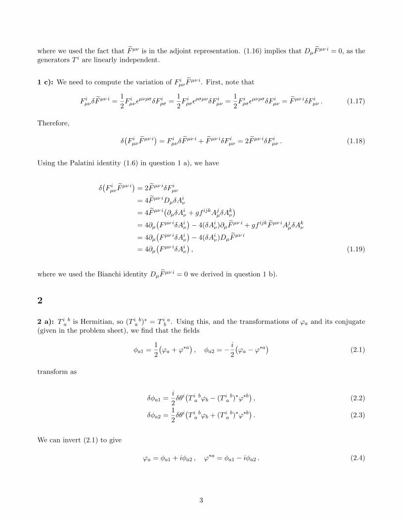
1 c): We need to compute the variation of F iµνFµν i. First, note that
F iµνδFµν i =
1
2F iµνε
µνρσδF iρσ =1
2F iρσε
ρσµνδF iµν =1
2F iρσε
µνρσδF iµν = Fµν iδF iµν . (1.17)
Therefore,
δ(F iµνF
µν i)
= F iµνδFµν i + Fµν iδF iµν = 2Fµν iδF iµν . (1.18)
Using the Palatini identity (1.6) in question 1 a), we have
δ(F iµνF
µν i)
= 2Fµν iδF iµν
= 4Fµν iDµδAiν
= 4Fµν i(∂µδA
iν + gf ijkAjµδA
kν
)= 4∂µ
(Fµν iδAiν
)− 4(δAiν)∂µF
µν i + gf ijkFµν iAjµδAkν
= 4∂µ(Fµν iδAiν
)− 4(δAiν)DµF
µν i
= 4∂µ(Fµν iδAiν
), (1.19)
where we used the Bianchi identity DµFµν i = 0 we derived in question 1 b).
2
2 a): T i ba is Hermitian, so (T i ba )∗ = T i ab . Using this, and the transformations of ϕa and its conjugate(given in the problem sheet), we find that the fields
φa1 =1
2
(ϕa + ϕ∗a
), φa2 = − i
2
(ϕa − ϕ∗a
)(2.1)
transform as
δφa1 =i
2δθi(T i ba ϕb − (T i ba )∗ϕ∗b
), (2.2)
δφa2 =1
2δθi(T i ba ϕb + (T i ba )∗ϕ∗b
). (2.3)
We can invert (2.1) to give
ϕa = φa1 + iφa2 , ϕ∗a = φa1 − iφa2 . (2.4)
3

Substituting this into the transformations, we find
δφa1 = −δθi(
Im(T i ba )φb1 + Re(T i ba )φb2), (2.5)
δφa2 = δθi(
Re(T i ba )φb1 − Im(T i ba )φb2). (2.6)
We can package φa1 and φa2 into a 2n component vector φa:
φa =
(φa1φa2
)(2.7)
which will transform under the real representation as
δφa = −δθi(
Im(T i ba )φb1 + Re(T i ba )φb2−Re(T i ba )φb1 + Im(T i ba )φb2
). (2.8)
We know, however, that
δφa = iδθi(T irealφ)a . (2.9)
where T ireal are the generators in the real representation. From (2.8), we can read off these generators to be
T ireal = i
(Im(T i ba ) Re(T i ba )−Re(T i ba ) Im(T i ba )
), (2.10)
which are purely imaginary, antisymmetric 2n× 2n matrices.
2 b): Define Sij = (T iφ, T jφ), where T i is purely imaginary and antisymmetric, and φ is real.
Symmetric: Since (u, v) = (v, u), Sij = (T iφ, T jφ) = (T jφ, T iφ) = Sji.
Real: (Sij)∗ = (T i∗φ, T j∗φ) = (−T iφ,−T jφ) = Sij , as T i is imaginary.
Since Sij is symmetric and real, it is diagonalisable with
S = ODOT , (2.11)
where O is the orthogonal matrix constructed by the orthonormal eigenvectors of S, and D is the diagonalmatrix of the eigenvalues of S. The mass squared matrix M2 is proportional to S, so if
M2(T iφ) = 0 , T iφ 6= 0 , (2.12)
for some values of i, then ϕi = T iφ satisfies
Sϕi = 0 . (2.13)
4
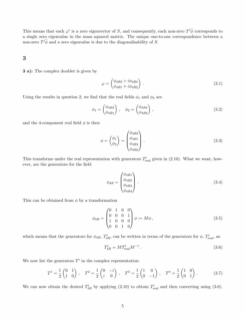
This means that each ϕi is a zero eigenvector of S, and consequently, each non-zero T iφ corresponds toa single zero eigenvalue in the mass squared matrix. The unique one-to-one correspondence between anon-zero T iφ and a zero eigenvalue is due to the diagonalisability of S.
3
3 a): The complex doublet is given by
ϕ =
(φ4R3 + iφ4R4
φ4R1 + iφ4R2
). (3.1)
Using the results in question 2, we find that the real fields φ1 and φ2 are
φ1 =
(φ4R3
φ4R1
), φ2 =
(φ4R4
φ4R2
), (3.2)
and the 4-component real field φ is then
φ =
(φ1φ2
)=
φ4R3
φ4R1
φ4R4
φ4R2
. (3.3)
This transforms under the real representation with generators T ireal given in (2.10). What we want, how-ever, are the generators for the field
φ4R =
φ4R1
φ4R2
φ4R3
φ4R4
. (3.4)
This can be obtained from φ by a transformation
φ4R =
0 1 0 00 0 0 11 0 0 00 0 1 0
φ := Mφ , (3.5)
which means that the generators for φ4R, T i4R, can be written in terms of the generators for φ, T ireal, as
T i4R = MT irealM−1 . (3.6)
We now list the generators T i in the complex representation:
T 1 =1
2
(0 11 0
), T 2 =
1
2
(0 −ii 0
), T 3 =
1
2
(1 00 −1
), T 4 =
1
2
(1 00 1
). (3.7)
We can now obtain the desired T i4R by applying (2.10) to obtain T ireal and then converting using (3.6).
5
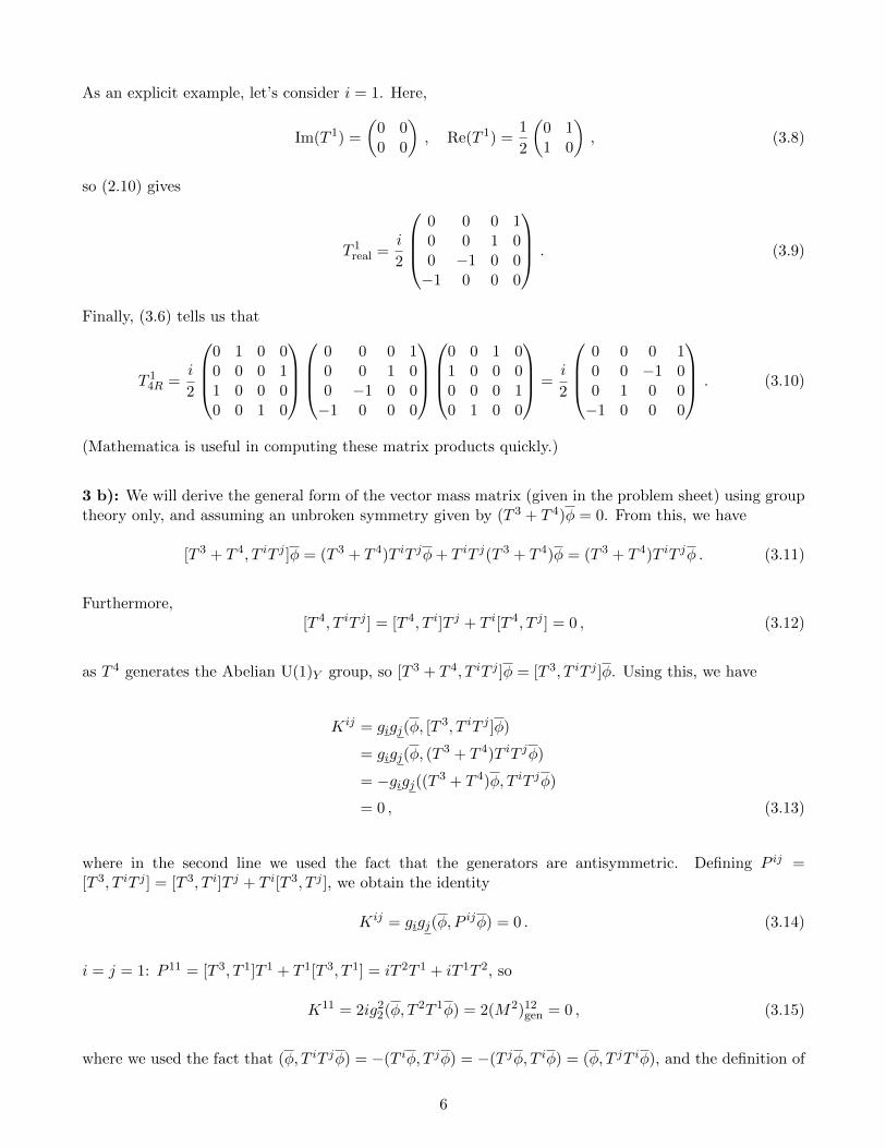
As an explicit example, let’s consider i = 1. Here,
Im(T 1) =
(0 00 0
), Re(T 1) =
1
2
(0 11 0
), (3.8)
so (2.10) gives
T 1real =
i
2
0 0 0 10 0 1 00 −1 0 0−1 0 0 0
. (3.9)
Finally, (3.6) tells us that
T 14R =
i
2
0 1 0 00 0 0 11 0 0 00 0 1 0
0 0 0 10 0 1 00 −1 0 0−1 0 0 0
0 0 1 01 0 0 00 0 0 10 1 0 0
=i
2
0 0 0 10 0 −1 00 1 0 0−1 0 0 0
. (3.10)
(Mathematica is useful in computing these matrix products quickly.)
3 b): We will derive the general form of the vector mass matrix (given in the problem sheet) using grouptheory only, and assuming an unbroken symmetry given by (T 3 + T 4)φ = 0. From this, we have
[T 3 + T 4, T iT j ]φ = (T 3 + T 4)T iT jφ+ T iT j(T 3 + T 4)φ = (T 3 + T 4)T iT jφ . (3.11)
Furthermore,[T 4, T iT j ] = [T 4, T i]T j + T i[T 4, T j ] = 0 , (3.12)
as T 4 generates the Abelian U(1)Y group, so [T 3 + T 4, T iT j ]φ = [T 3, T iT j ]φ. Using this, we have
Kij = gigj(φ, [T3, T iT j ]φ)
= gigj(φ, (T3 + T 4)T iT jφ)
= −gigj((T 3 + T 4)φ, T iT jφ)
= 0 , (3.13)
where in the second line we used the fact that the generators are antisymmetric. Defining P ij =[T 3, T iT j ] = [T 3, T i]T j + T i[T 3, T j ], we obtain the identity
Kij = gigj(φ, Pijφ) = 0 . (3.14)
i = j = 1: P 11 = [T 3, T 1]T 1 + T 1[T 3, T 1] = iT 2T 1 + iT 1T 2, so
K11 = 2ig22(φ, T 2T 1φ) = 2(M2)12gen = 0 , (3.15)
where we used the fact that (φ, T iT jφ) = −(T iφ, T jφ) = −(T jφ, T iφ) = (φ, T jT iφ), and the definition of
6
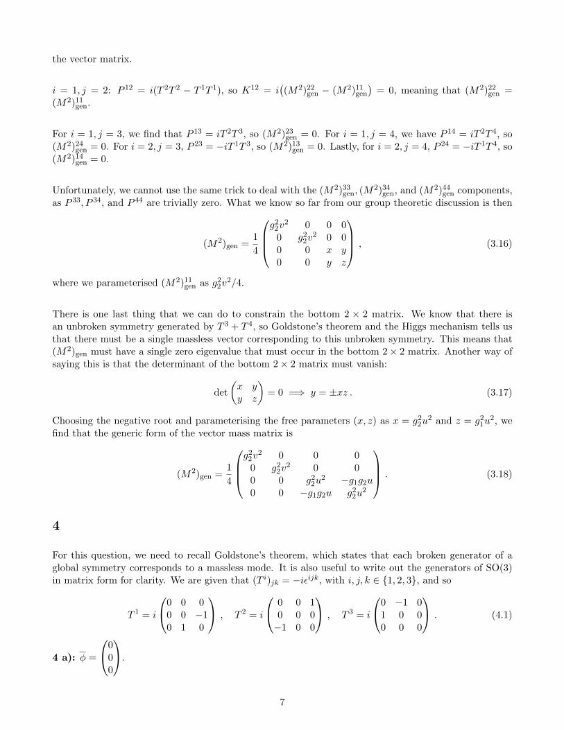
the vector matrix.
i = 1, j = 2: P 12 = i(T 2T 2 − T 1T 1), so K12 = i((M2)22gen − (M2)11gen
)= 0, meaning that (M2)22gen =
(M2)11gen.
For i = 1, j = 3, we find that P 13 = iT 2T 3, so (M2)23gen = 0. For i = 1, j = 4, we have P 14 = iT 2T 4, so(M2)24gen = 0. For i = 2, j = 3, P 23 = −iT 1T 3, so (M2)13gen = 0. Lastly, for i = 2, j = 4, P 24 = −iT 1T 4, so(M2)14gen = 0.
Unfortunately, we cannot use the same trick to deal with the (M2)33gen, (M2)34gen, and (M2)44gen components,
as P 33, P 34, and P 44 are trivially zero. What we know so far from our group theoretic discussion is then
(M2)gen =1
4
g22v
2 0 0 00 g22v
2 0 00 0 x y0 0 y z
, (3.16)
where we parameterised (M2)11gen as g22v2/4.
There is one last thing that we can do to constrain the bottom 2 × 2 matrix. We know that there isan unbroken symmetry generated by T 3 + T 4, so Goldstone’s theorem and the Higgs mechanism tells usthat there must be a single massless vector corresponding to this unbroken symmetry. This means that(M2)gen must have a single zero eigenvalue that must occur in the bottom 2× 2 matrix. Another way ofsaying this is that the determinant of the bottom 2× 2 matrix must vanish:
det
(x yy z
)= 0 =⇒ y = ±xz . (3.17)
Choosing the negative root and parameterising the free parameters (x, z) as x = g22u2 and z = g21u
2, wefind that the generic form of the vector mass matrix is
(M2)gen =1
4
g22v
2 0 0 00 g22v
2 0 00 0 g22u
2 −g1g2u0 0 −g1g2u g22u
2
. (3.18)
4
For this question, we need to recall Goldstone’s theorem, which states that each broken generator of aglobal symmetry corresponds to a massless mode. It is also useful to write out the generators of SO(3)in matrix form for clarity. We are given that (T i)jk = −iεijk, with i, j, k ∈ {1, 2, 3}, and so
T 1 = i
0 0 00 0 −10 1 0
, T 2 = i
0 0 10 0 0−1 0 0
, T 3 = i
0 −1 01 0 00 0 0
. (4.1)
4 a): φ =
000
.
7
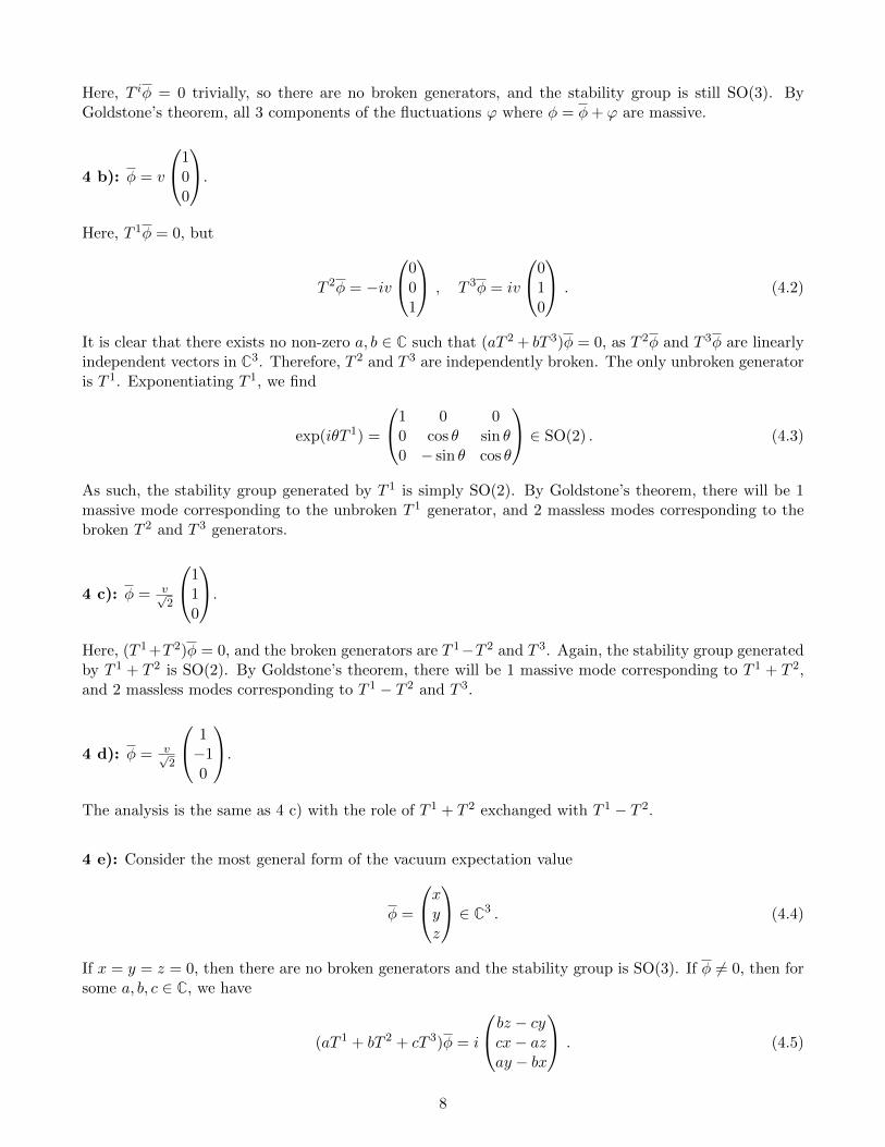
Here, T iφ = 0 trivially, so there are no broken generators, and the stability group is still SO(3). ByGoldstone’s theorem, all 3 components of the fluctuations ϕ where φ = φ+ ϕ are massive.
4 b): φ = v
100
.
Here, T 1φ = 0, but
T 2φ = −iv
001
, T 3φ = iv
010
. (4.2)
It is clear that there exists no non-zero a, b ∈ C such that (aT 2 + bT 3)φ = 0, as T 2φ and T 3φ are linearlyindependent vectors in C3. Therefore, T 2 and T 3 are independently broken. The only unbroken generatoris T 1. Exponentiating T 1, we find
exp(iθT 1) =
1 0 00 cos θ sin θ0 − sin θ cos θ
∈ SO(2) . (4.3)
As such, the stability group generated by T 1 is simply SO(2). By Goldstone’s theorem, there will be 1massive mode corresponding to the unbroken T 1 generator, and 2 massless modes corresponding to thebroken T 2 and T 3 generators.
4 c): φ = v√2
110
.
Here, (T 1+T 2)φ = 0, and the broken generators are T 1−T 2 and T 3. Again, the stability group generatedby T 1 + T 2 is SO(2). By Goldstone’s theorem, there will be 1 massive mode corresponding to T 1 + T 2,and 2 massless modes corresponding to T 1 − T 2 and T 3.
4 d): φ = v√2
1−10
.
The analysis is the same as 4 c) with the role of T 1 + T 2 exchanged with T 1 − T 2.
4 e): Consider the most general form of the vacuum expectation value
φ =
xyz
∈ C3 . (4.4)
If x = y = z = 0, then there are no broken generators and the stability group is SO(3). If φ 6= 0, then forsome a, b, c ∈ C, we have
(aT 1 + bT 2 + cT 3)φ = i
bz − cycx− azay − bx
. (4.5)
8

For the combination aT 1 + bT 2 + cT 3 to be an unbroken generator, we require the RHS of (4.5) to vanish.This requires solving the following 3 linear, simultaneous equations for the parameters a, b, c:
bz = cy , cx = az , ay = bx . (4.6)
Without loss of generality, let’s assume x 6= 0 and a 6= 0. Then, the last two equations can be solved by
c =az
x, b =
ay
x. (4.7)
With this expressions for c and b, we find that the first equation bz = cy is trivially satisfied:
bz − cy =ayz
x− azy
x= 0 . (4.8)
We have now found a unique solution for the unbroken generator, and it is given by
a(T 1 +
y
xT 2 +
z
xT 3)
(4.9)
Since a 6= 0, we can ignore the overall factor of a. The broken generators are formed by linearly inde-pendent combinations of T i that are orthogonal to the unbroken generator, and since there’s only oneunbroken generator, there must be two broken one. After a bit of algebra, we find that one particularbasis for the broken generators is
Unbroken: T 1 = T 1 +y
xT 2 +
z
xT 3 (4.10)
Broken: T 2 =y
xT 1 − T 2 , T 3 =
z
xT 1 +
yz
x2T 2 −
(1 +
y2
x2
)T 3 . (4.11)
Let’s just check that this works for the cases we talked about. For 4 b), we had x = v, y = 0, z = 0, sothe unbroken generator is T 1 = T 1, and the broken generators are T 2 = T 2, and T 3 = T 3. For 4 c), wehad x = v/
√2, y = x, z = 0, so T 1 = T 1 + T 2, T 2 = T 1 − T 2, and T 3 = −2T 3. Finally, for 4 d), we had
x = v/√
2, y = −x, z = 0, so T 1 = T 1 − T 2, T 2 = −(T 1 + T 2), and T 3 = −2T 3.
5
5 a): Let M ∈ GL(n,C) and define K = M †M . Clearly, K† = (M †M)† = K, so K is Hermitian, whichmeans that it has a set of non-zero eigenvectors ei, i ∈ {1, . . . , n}, with real eigenvalues Kei = λiei,λi ∈ R. The eigenvectors are orthonormal with respect to the Cn inner product
(ei, ej) =
n∑α=1
(eαi )∗eαj = δij , (5.1)
where eαi is the αth component of ei. By orthonormality,
λi = (ei,Kei) = (ei,M†Mei) = (Mei,Mei) = ||Mei||2 ≥ 0 , (5.2)
9
where we used the definition of the Hermitian conjugate: (u,Mv) = (M †u, v). This shows that theeigenvalues are strictly positive unless Mei = 0, which is a case we will ignore, and we shall write themas λi = ω2
i , with ωi ∈ R \ {0}.
To diagonalise K, construct the matrix U = (e1, e2, . . . , en), where we treat ei as column vectors. Byorthonormality of the eigenvectors, we see that
U †U = UU † = 1n , (5.3)
so U is unitary. Therefore,
K = K(UU †) = (KU)U † . (5.4)
By defining the diagonal matrix
D2 = diag(ω21, ω
22, . . . , ω
2n) , (5.5)
we have
KU = K(e1, e2, . . . , en) = (ω21e1, ω
22e2, . . . , ω
2nen) = UD2 . (5.6)
Thus,
K = UD2U † . (5.7)
5 b): Define H = UDU †. To compute H−1, note that since ωi 6= 0,
Dm = diag(ωm1 , ωm2 , . . . , ω
mn ) (5.8)
for any m ∈ Z. This, combined with the unitarity of U then implies that
H−1 = UD−1U † . (5.9)
Now, define U = MH−1 = MUD−1U †. Then,
U †U = UD−1U †M †MUD−1U †
= UD−1U †(UD2U †
)UD−1U †
= 1n , (5.10)
where we used the result in 5 a) that K = M †M = UD2U †. This means that U is unitary. With thesedefinitions, we can now define the matrix V = UU = MUD−1, which is unitary because it is the productof unitary matrices. Then,
V †MU = D−1U †M †MU = D−1U †(UD2U †
)U = D . (5.11)
10

This can be rewritten as
M = V DU † . (5.12)
Note that if M is Hermitian, then
M = M † =⇒ V DU † = UDV † =⇒ V = U , (5.13)
giving the usual result for the diagonalisation of a Hermitian matrix.
6
Let A,B,C ∈ C satisfy A + B + C = 0. It is useful to write A = aeiα, B = beiβ and C = ceiγ , wherea, b, c ∈ R+ and α, β, γ ∈ [0, 2π). Consider a triangle with vertices on (0, 0), A and A + B = −C. Thediagram will look like this:
Clearly, θ = γ − α− π, and the height h = a| sin θ|. The area is then
Area =1
2ac| sin θ| . (6.1)
Now,
| Im(AC∗)| = | Im(acei(α−γ)
)| = ac| − Im ei(α−γ+π)| = ac| sin θ| =⇒ Area =
1
2| Im(AC∗)| . (6.2)
Since B = −(A + C), | Im(BC∗)| = | Im(AC∗) + Im(CC∗)| = | Im(AC∗)|, as CC∗ ∈ R. Similarly,| Im(AB∗)| = | Im(AA∗) + Im(AC∗)| = | Im(AC∗)|. Thus,
Area =1
2| Im(AC∗)| = 1
2| Im(BC∗)| = 1
2| Im(AB∗)| . (6.3)
11