solverstat: the manual - webs

1

SOLVERSTAT:

THE MANUAL

September 10, 2010

Version 0.1b

(PROOF)

By: Pierluigi Polese

2

This is only a proof release of the manual. My English is bad and I will appreciate your

corrections and notes. I also greatly appreciate suggestion about SolverStat.

If you like this software, please cite as:

"SOLVERSTAT : a new utility for multipurpose analysis. An application to the investigation of

dioxygenated Co(II) complex formation in dimethylsulfoxide solution."

C.Comuzzi, P.Polese, A.Melchior, R.Portanova, M.Tolazzi.

Talanta 59 (2003) 67-80

Many Thanks

Pierluigi Polese

[email protected]

[email protected]

3

INDEX

1 SOLVERSTAT INSTALLATION ................................................................................................6

1.1 Excel 97, 2000 .................................................................................................................6

1.2 Excel XP, 2003 ................................................................................................................7

1.3 Excel 2007 .......................................................................................................................8

2 THE EXCEL SOLVER ...........................................................................................................13

2.1 Activation and Installation ............................................................................................13

2.2 SomeTHing about Solver...............................................................................................14

2.2.1 The Solver Parameters dialog box ........................................................................14

2.2.2 The Options Parameters dialog box ......................................................................15

3 LEAST SQUARES REGRESSION ............................................................................................17

3.1 Local minima.................................................................................................................18

3.2 Model building and Regression analysis ......................................................................19

4 SOLVERSTAT......................................................................................................................22

4.1 Main Level.....................................................................................................................22

4.1.1 New Sheet .............................................................................................................22

4.1.2 Set Solver ..............................................................................................................23

4.1.3 Run Solver.............................................................................................................23

4.1.4 Regression Statistic ...............................................................................................23

4.1.5 MC Solver .............................................................................................................23

4.1.6 Linear Regression..................................................................................................24

4.1.7 Uncertainty Propagation IRWLS ..........................................................................24

4.1.8 Remove SolverStat ................................................................................................24

4.2 Regression Reliability ...................................................................................................25

4.2.1 Asymmetric Confidence Interval ..........................................................................25

4.2.2 Beale MCMC Confidence Regions.......................................................................25

4.2.3 Monte Carlo Simulation ........................................................................................25

4.2.4 Bootstrap the Observations ...................................................................................26

4.2.5 Bootstrap the Weighted Residuals ........................................................................26

4.2.6 Associated Simulation...........................................................................................26

4.2.7 Repeat Parameters Distribution Statistics .............................................................27

4.2.8 LOO Cross-Validation ..........................................................................................27

4.2.9 MC Cross Validation.............................................................................................27

4.3 Analysis .........................................................................................................................28

4.3.1 Power.....................................................................................................................28

4.3.2 Significance...........................................................................................................28

4.3.3 Observation Diagnostics .......................................................................................29

4.4 ROBUST Regression .....................................................................................................29

4.4.1 IRLS ......................................................................................................................30

4.4.2 LTS........................................................................................................................30

4.4.3 LMS.......................................................................................................................30

4.5 LOGISTIC Regression...................................................................................................31

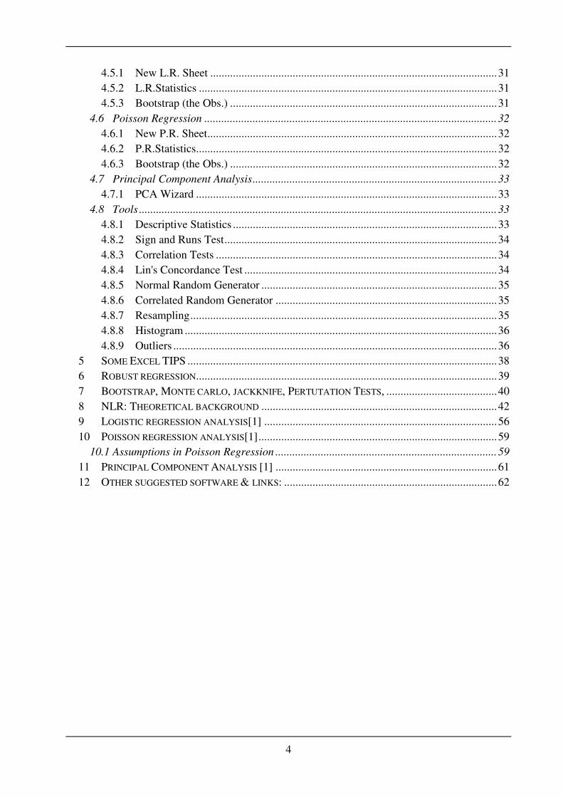
4

4.5.1 New L.R. Sheet .....................................................................................................31

4.5.2 L.R.Statistics .........................................................................................................31

4.5.3 Bootstrap (the Obs.) ..............................................................................................31

4.6 Poisson Regression .......................................................................................................32

4.6.1 New P.R. Sheet......................................................................................................32

4.6.2 P.R.Statistics..........................................................................................................32

4.6.3 Bootstrap (the Obs.) ..............................................................................................32

4.7 Principal Component Analysis......................................................................................33

4.7.1 PCA Wizard ..........................................................................................................33

4.8 Tools ..............................................................................................................................33

4.8.1 Descriptive Statistics .............................................................................................33

4.8.2 Sign and Runs Test................................................................................................34

4.8.3 Correlation Tests ...................................................................................................34

4.8.4 Lin's Concordance Test .........................................................................................34

4.8.5 Normal Random Generator ...................................................................................35

4.8.6 Correlated Random Generator ..............................................................................35

4.8.7 Resampling............................................................................................................35

4.8.8 Histogram ..............................................................................................................36

4.8.9 Outliers ..................................................................................................................36

5 SOME EXCEL TIPS .............................................................................................................38

6 ROBUST REGRESSION..........................................................................................................39

7 BOOTSTRAP, MONTE CARLO, JACKKNIFE, PERTUTATION TESTS, .......................................40

8 NLR: THEORETICAL BACKGROUND ...................................................................................42

9 LOGISTIC REGRESSION ANALYSIS[1] ..................................................................................56

10 POISSON REGRESSION ANALYSIS[1]....................................................................................59

10.1 Assumptions in Poisson Regression ..............................................................................59

11 PRINCIPAL COMPONENT ANALYSIS [1] ..............................................................................61

12 OTHER SUGGESTED SOFTWARE & LINKS: ...........................................................................62

6

1 SOLVERSTAT INSTALLATION

1.1 EXCEL 97, 2000

For Excel 97 go to step 9.

1. Open Microsoft Excel and click on the TOOLS Menu Bar Selection.

2. Click on the MACRO selection on the drop down menu.

3. Click on the SECURITY tab.

5. On the SECURIT LEVEL tab activate the MEDIUM Security radio button.

7

6. Click on the TRUSTED PUBLISHERS tab.

7. Enable TRUST ALL INSTALLED ADD-INS AND TEMPLATE

8. Click OK.

9. Launch Solverstat.xla and click ENABLE MACROS.

That is all.

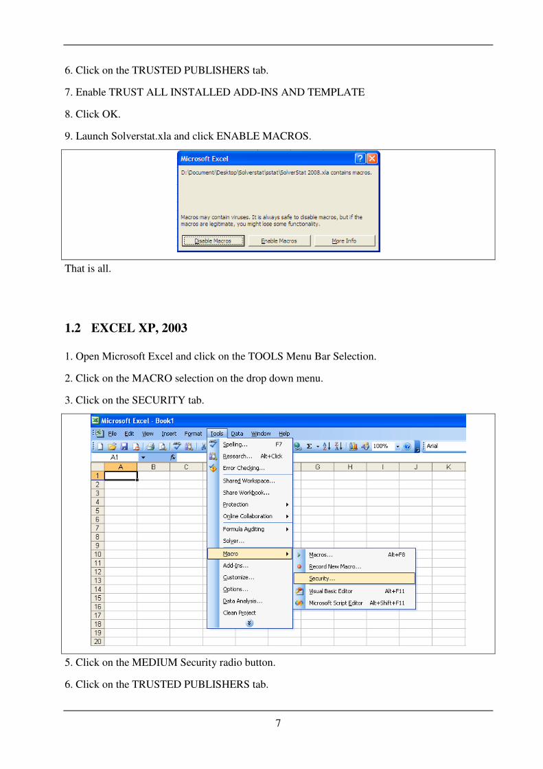
1.2 EXCEL XP, 2003

1. Open Microsoft Excel and click on the TOOLS Menu Bar Selection.

2. Click on the MACRO selection on the drop down menu.

3. Click on the SECURITY tab.

5. Click on the MEDIUM Security radio button.

6. Click on the TRUSTED PUBLISHERS tab.

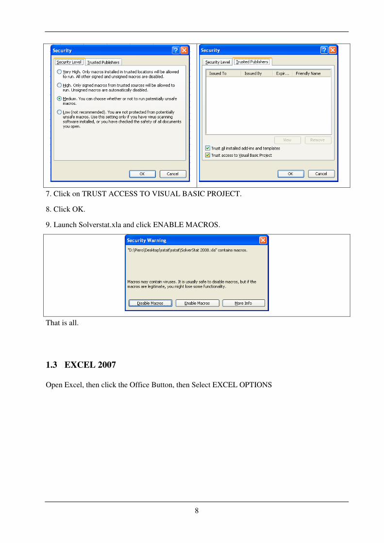
8

7. Click on TRUST ACCESS TO VISUAL BASIC PROJECT.

8. Click OK.


That is all.

1.3 EXCEL 2007

Open Excel, then click the Office Button, then Select EXCEL OPTIONS

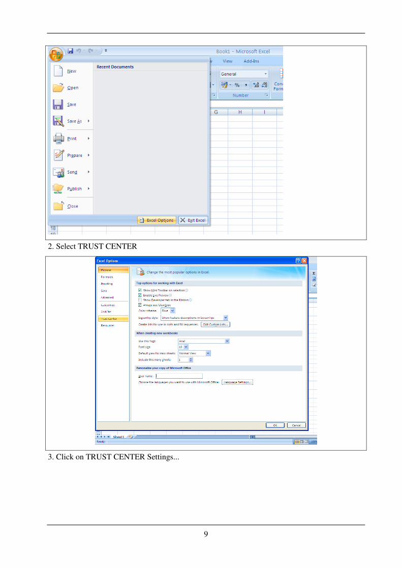
9

2. Select TRUST CENTER

3. Click on TRUST CENTER Settings...

10

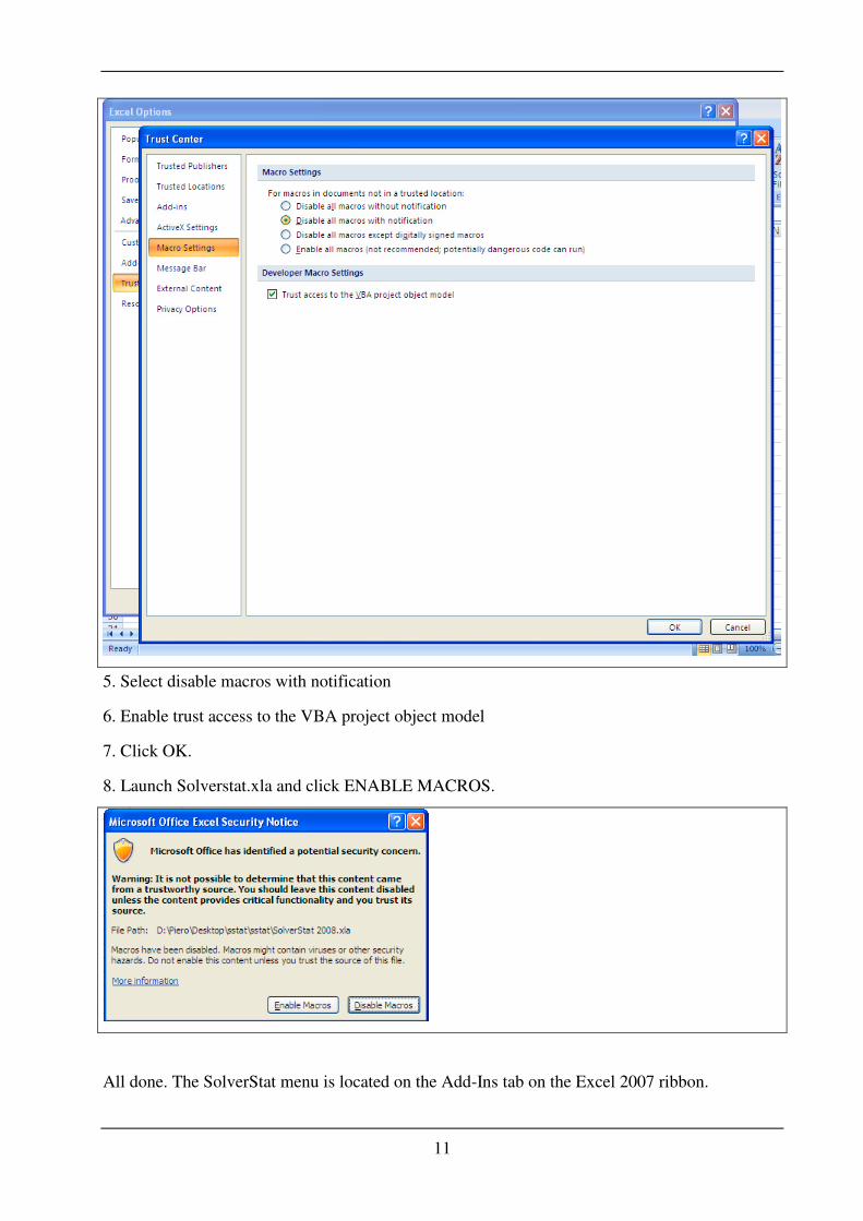
4. Select MACRO SETTINGS

11

5. Select disable macros with notification

6. Enable trust access to the VBA project object model

7. Click OK.


All done. The SolverStat menu is located on the Add-Ins tab on the Excel 2007 ribbon.

13

2 THE EXCEL SOLVER

The Solver is an optimization package that may be used for finding the optimal solution of your

model according to the conditions that you determine. The Solver finds a maximum, minimum

or specified value of a target cell by varying the values in one or several changing cells. It

accomplishes this by means of an iterative process, beginning with trial values of the

coefficients. The value of each coefficient is changed by a suitable increment, the new value of

the function is calculated and the change in the value of the function is used to calculate

improved values for each of the coefficients. The process is repeated until the desired result is

obtained. The Solver uses gradient methods or the simplex method to find the optimum set of

coefficients.

There are many published computer programs and commercial software packages that perform

non-linear regression analysis, but you can obtain the same results very easily by using the

Solver. With good starting values, when applied to the same data set, the Solver gives the same

results as commercial software packages.

2.1 ACTIVATION AND INSTALLATION

From the Tools menu, select the Solver option.

If you don't see the option in Excel, select Tools, Add-Ins.

From the list, choose Solver Add-in. The option is now going to appear in the menu tools.

If Solver Add-in is not on your list of available Add-Ins, you will need your Microsoft Office

CD-ROM. Put the CD in. If the CD doesn't run its setup program automatically, open My

Computer, find setup.exe on the CD and double-click it to run it.

14

Click the Add or Remove Features button. In the graphic that then appears, click the little plus

sign next to Microsoft Excel for Windows. This opens up the outline under that box. Click the

little plus sign next to Add-ins to open that list up. Look down that list and you should find

Solver. Click on Solver and choose Run from My Computer, so that the box is white, with no

yellow "1".

While you're here, you might want to get the Analysis ToolPak, too. It's not required for

Solverstat, but it may be useful. It provides an alternative method for doing linear regressions.

Then click Update Now to proceed with the installation.

2.2 SOMETHING ABOUT SOLVER

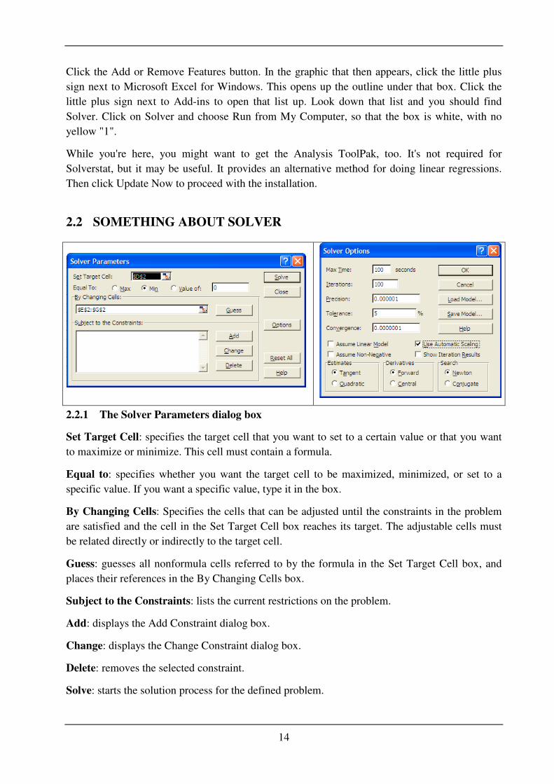
2.2.1 The Solver Parameters dialog box

Set Target Cell: specifies the target cell that you want to set to a certain value or that you want

to maximize or minimize. This cell must contain a formula.

Equal to: specifies whether you want the target cell to be maximized, minimized, or set to a

specific value. If you want a specific value, type it in the box.

By Changing Cells: Specifies the cells that can be adjusted until the constraints in the problem

are satisfied and the cell in the Set Target Cell box reaches its target. The adjustable cells must

be related directly or indirectly to the target cell.

Guess: guesses all nonformula cells referred to by the formula in the Set Target Cell box, and

places their references in the By Changing Cells box.

Subject to the Constraints: lists the current restrictions on the problem.

Add: displays the Add Constraint dialog box.

Change: displays the Change Constraint dialog box.

Delete: removes the selected constraint.

Solve: starts the solution process for the defined problem.

15

Close: closes the dialog box without solving the problem. Retains any changes you made by

using the Options, Add, Change, or Delete buttons.

Options: Displays the Solver Options dialog box, where you can load and save problem models

and control advanced features of the solution process.

Reset All: clears the current problem settings, and resets all settings to their original values.

For a lest squares regression you must activate the Equal to option to MIN; instead in the care

of logistic regression you must activate the MAX option.

2.2.2 The Options Parameters dialog box

The Load Model and Save Model buttons enable the user to recall and retain model settings so

they don't need to be re-entered every time the optimization is run.

Max time limits the time taken to find the solution (in seconds). The default 100 seconds should

be appropriate for standard linear problems.

Iterations restricts the number of iterations the algorithm can use to find a solution

Precision is used to determine the accuracy with which the value of a constraint meets a target

value. A fractional number between 0 (zero) and 1 The higher the precision, the smaller the

number (i.e. .01 is less precise than .0001)

Tolerance applies only to integer constraints, and is used to estimate the level of tolerance (as a

percentage) by which the solution satisfying the constraints can differ from the true optimal

value and still be considered acceptable. In other words, the lower the tolerance level, the longer

it will take for the solutions to be acceptable.

Convergence applies only to non-linear models and is a fractional number between 0 and 1. If

after five iterations the relative change in the objective function is less than the convergence

specified, Solver stops. As with precision and tolerance, the smaller the convergence number the

longer it will take to find a solution (up to Max Time that is).

Lowering Precision, Tolerance, and Convergence values will slow down the optimization but it

may help the algorithm to find a solution. In general, these defaults should be changed if Solver

is experiencing problems finding an optimal solution.

Assume Linear Model is a very important choice. If the optimization problem is truly linear,

then this option should be chosen because Solver will use the Simplex method, which should

find a solution faster and be more robust than the default optimization method. However, the

function has to be truly linear for this option to be used. Solver has a built-in algorithm that

checks for linearity conditions, but the analyst should not rely solely on this to asses the model

structure.

Show Iteration Results: when this option is selected, Solver will pause to show the result of

each iteration, and will require user-input to reinitiate the next iteration. This option is certainly

not recommended for computing intensive optimization.

16

Use Automatic Scaling when selected will rescale the variable in cases where variables and

results have large differences in magnitude

Assume Non-Negative will bound to zero all the decision variables that have not been explicitly

constrained. It is preferable however to specify explicitly the variables boundaries in the model.

The Estimates section allows to use either a Tangent method or Quadratic method to estimate

the optimal solution. The Tangent method extrapolates from a tangent vector, whereas Quadratic

are the method of choice for highly non-linear problems.

The Derivatives section specifies the differencing method used to estimate partial derivatives of

objective and constraint functions (when differentiable, of course). In general, Forward should be

used for most problems where the constraint values change slowly, whereas Central method

should be used when the constraints change more dynamically. The Central method can be

chosen when solver can not find improving solutions.

Finally, the Search section allows one to specify the algorithm used to determine the direction to

search at each iteration. The options are Newton which is a quasi-Newton method to be used

when speed is an issue and computer power is a limiting factor, Conjugate is the preferred

method when memory is an issue, but speed can be slightly compromised.

Typically for a regression using Solver, you set the Convergence to little number such 1E-7 and

activate the Automatic Scaling option.

17

3 LEAST SQUARES REGRESSION

Regression analysis is a statistical technique used to determine whether experimental variables

are interdependent and to express quantitatively the relationship between them, and the degree of

correlation. For most chemical systems, the mathematical form of the equation relating the

dependent and independent variables is known; the goal is to obtain the values of the coefficients

in the equation - the regression coefficients. In other cases, the data may be fitted by an empirical

fitting function such as a power series, simply for purposes of graphing or interpolation. In any

event, you must provide the form of the equation; regression analysis merely provides the

coefficients.

The method of least squares yields the parameters that minimize the sum of squares of the

residuals (the deviation of each measurement of the dependent variable from its calculated

value).

∑ −=n

calcobsd yyRSS1

2)( ( 3.1a )

To Use the Solver to Perform a Least-Squares Curve Fitting

1. Start with a worksheet containing the data (one or more independent variable x and one

dependent variable yobsd) to be fitted.

2. Add a row containing one or more coefficients b to be varied.

3. Add a column on the right of yobsd containing ycalc values, calculated by means of an

appropriate formula and involving the x values and the coefficients to be varied.

4. Add a column to calculate the square of the residual (yobsd-ycalc) for each data point.

5. Calculate in a cell the sum of squares of the residuals.

6. Call the Solver (Use TOOLS -> SOLVER) to minimize the sum of squares of residuals (the

target cell) by changing the coefficients of the function (the changing cells).

7. Click on OPTIONS and set the CONVERGENCE to 1E-7 and activate the AUTOMATIC

SCALING option. Click OK to close the options box.

8. Click OK to start the minimization

9. After a while the program will come to a halt, announce that it has converged on a solution,

and ask you whether it should keep that solution, or put the starting guess values back

The procedure New Sheet in SolverStat guide you in the preparation of a new sheet useful for

doing least squares regression.

18

3.1 LOCAL MINIMA

A big problem with Solver and other minimization routines, is that they may betrapped in a local

minimum. This happens when the model is highly nonlinear or data are noisy and starting values

are far from the best estimates.

To prevent this problem, Solver should be run several times with different starting parameter

values. A number of indicators can assist in identifying a local minimum, though there is no

‘fool-proof’ way of deciding whether a local or global minimum has been discovered. For

example when a local minimum in RSS is found, the standard errors in the parameter estimates

tend to be large. Check also whether they make sense scientifically.

There are no general rules that may be applied in order to determine good starting values for

parameter estimates prior to fitting by non-linear least squares, but you can use some tricks such us:

1. plot the data and interpret the behavior of the function in terms of the parameters;

2. interpret the behavior of derivatives of the model function in terms of the parameters

analytically or graphically;

3. transform the model function analytically or graphically to obtain simpler, preferably linear,

behaviour (e.g. linearize the equation);

4. reduce the dimensions by substituting values for some parameters or by evaluating the

function at specific design values.

19

3.2 MODEL BUILDING AND REGRESSION ANALYSIS

A secondary but no less important goal is to obtain the standard deviations of the regression

parameters, and an estimate of the goodness of fit of the data to the model equation. The Solver

of Microsoft Excel yields minimized parameters but provides no estimates of their precision and

an incomplete and unprompted statistical analysis of fittings: the statistical analysis of the results

is on the other hand, a crucial step to evaluate the reliability of the whole model. SolverStat

overcome the Excel limitations through various procedures.

The next procedure can therefore be used for the regression model building:

(i) Proposal of a model from theory and preliminary exploration of data

(ii) Make the regression model

(iii) Run regression and statistic

(iv) Conduct the triplet analysis.

(a) If after examination of data quality, some outliers are found and deleted, go to (iii)

(b) If after examination of model quality some parameters are omitted go to (ii)

(c) if the examination of regression method evidences the necessity of corrective action,

take opportune remedial measures and go to (ii)

(v) If more than one model is selected and not discarded by the regression triplet, then

conduct a model discrimination.

The next table summarize statistical requirements

20

Data quality

Leverages (influential points) <3p/n

Studentized deleted residuals (outliers) <3

Williams plot (influential outliers)

Robust Regression (outliers)

Model quality

Regression:

Model F-Test (significativity of regression) »1

Runs of sign (systematic deviation of curvefrom data points) ~n/2

Parameters

Student t test (significativity of parameter) *0

Confidence intervals CI (significativity of

parameter)

*0

Monte Carlo MC (nonlinearity effects) CI ~ MC CI

Regression method quality

(regression assumptions)

VIF (Multicollinearity in multiple regressions) <10

Shapiro Wilk test (normality of residuals) Probability

Jarque-Bera test (normality of residuals) Probability

Levene F-test (homoscedasticity or residuals) Probability

Durbin-Watson test (independence of residuals) ~2

Models discrimination

R2 Highest

R2adjusted Highest

PRESS Smaller

Akaike information criteria AIC Smaller

RSS Smaller

F-test for models comparisons F>>l

22

4 SOLVERSTAT

4.1 MAIN LEVEL

4.1.1 New Sheet

Purpose: A wizard to create a sheet suitable to perform regression analysis using SolverStat.

Requirements: None at this stage.

Output: A new sheet ready to use to create a new least squares regression model.

Example: Create a new sheet for the regression of next data (Tutorials.xls, “Regression example

data”):

X Y

0 1.0

1 2.1

2 4.5

3 9.4

4 20.3

5 25.7

6 32.3

7 57.8

8 63.3

9 82.7

10 101.0

Run NEW SHEET, select one X series, two parameters b and no constants. At this stage a new

sheet properly formatted is produced. fill the X and Y cells with the above values, delete the

“SdX” and “SdY” label (or labels, if you prefer); delete “New Obs”, “Label” and “Track” labels,

copy down “Ycalc” and “r^2” formulas (first cells below these labels). The sheet is ready to

optimize.

Tips: Below the last X data (first X column on the left), you may use the label (keyword) “New

obs” and add below the label a series of new observations (X, Y, Ycalc formulas). You can use

also the label (keyword) “Track” and add a series of linked cells or formulas (for example

“=D6”) to record the cell values during simulations.

23

4.1.2 Set Solver

Purpose: When data and formulas are written, and the sheet is ready, this procedure set Solver

settings properly.

Requirements: Data and formulas written in a properly formatted sheet.

Output: Solver settings applied.

Example: Call SET SOLVER, after created the example in 4.1.1.

4.1.3 Run Solver

Purpose: Call the Solver dialog box once the worksheet is ready.

Requirements: An optimized regression sheet, ready to use.

Output: Optimized regression parameters.

Example: Change the value of a in the example of 4.1.2 to 0 and then call RUN SOLVER.

4.1.4 Regression Statistic

Purpose: Perform a complete statistical analysis of a least squares regression (unweighted or

weighted, linear or nonlinear).


Output: A new Excel sheet with a complete statistical analysis of a least squares regression.

Example: Run REGRESSION STATISTIC on example of 4.1.2. Observe the results: the Durbin

Watson Tests show a warning! Create a XY ploot and look the data! Copy the original regression

sheet and try to create a parabolic model (if you need, look the “Parabolic regression” example

sheet. Minimize and run again REGRESSION STATISTIC. Try again with a model without the

term b1 X.

4.1.5 MC Solver

Purpose: Obtain optimized regression parameters trough a Monte Carlo procedure applied to

Solver.


Output: Optimized regression parameters.

More information: This procedure is useful when there are relative minima in the model applied.

The New Sheet procedure create some cells to bound the MC SOLVER procedure: “MC Search

N” (the number of simulations), “Start Value” (the lower limits for the parameters) and “End

24

Value” the upper limits for the parameters). If these values are missing, SolverStat ask the user

for the number of simulations, for the “Exploration factor” (a random value for the parameter is

generated between βi / f and f βi) and the kT factor (a parameter used in the simulated annealing

procedure useful for very hard functions); in the last case, if a value of 0 is selected, the random

parameters are generated using a Markov chain (simply the new parameter are generated from

the last, adding a random quantity). For kT a suggested value is the value of RSS improvement

during optimization.

Example: Run MC SOLVER on example of 4.1.2.

4.1.6 Linear Regression

Purpose: compute parameter values using matrix algebra. Useful also for initial values in

nonlinear regressions.

Requirements: An optimized regression sheet, ready to use. Linear models

Output: Estimated parameter values for linear models.

Example: Run MC SOLVER on example of 4.1.2 after changing the optimized parameters to

random values.

4.1.7 Uncertainty Propagation IRWLS

Purpose: Estimation of regression parameters of models with measurement uncertainty in both

the regressed quantity and the independent variables or in the model constants. Estimation were

obtained using a Iteratively Reweighted Least Squares procedure.

Requirements: An optimized regression sheet, ready to use. Explicit standard deviations for

independent variables and/or model constants.

Output: A report sheet and a new regression sheet with IRWLS estimated parameters.

Additional information: The procedure is iterative; at each step new weights are computed on the

basis of asymptotic error propagation rules.

4.1.8 Remove SolverStat

Purpose: close SolverStat workbook.

Requirements: none

Output: none.

25

4.2 REGRESSION RELIABILITY

4.2.1 Asymmetric Confidence Interval

Purpose: compute asymmetric joint confidence intervals on the basis of the next statistic:

RSSj / [sy2 (n - p)] ≤ (1 + p / (n - p) FInv(α, p, n - p)

For absolute weighting, next formula is used:

RSSj / [sy2 (n - p)] ≤ (1 + p / (n - p) χ2

Inv(α, p)


Output: A new sheet with standard and asymmetric joint confidence intervals.

Additional information: Briefly, parameter of interest was kept constant at its best-fit value,

while all the remaining parameters were optimized. The resulting value of weighted least squares

was recorded. Subsequently the parameter of interest was shifted to a lower or to a higher value,

progressively away from the best-fit value. At each step, all the parameters were again subjected

to least-squares optimization. As the rate constant of interest moved away from its best-fit value,

the sum of least-square deviations naturally increased. Statistical theory gives us a critical value

of this increase in the sum of squares for each probability level of the confidence interval.

4.2.2 Beale MCMC Confidence Regions

Purpose: compute Beale Confidence Regions using a Monte Carlo approach on the basis of the

next statistic:

RSSj / [sy2 (n - p)] ≤ (1 + p / (n - p) FInv(α, p, n - p)

For absolute weighting, next formula is used:

RSSj / [sy2 (n - p)] ≤ (1 + p / (n - p) χ2

Inv(α, p)

A Markov-chain method is available to explore confidence regions.

Requirements: An optimized regression sheet, ready to use. If parameters range are unspecified,

a fraction of parameter value is used.

Output: A new sheet with accepted simulated parameter values. To obtain a graphical

representation, select two parameters of interest and create a x-y scatter plot.

4.2.3 Monte Carlo Simulation

Purpose: Perform a Monte Carlo simulation for the evaluation of confidence intervals of

determined parameters.

26

Requirements: An optimized regression sheet, ready to use. SD for y values must be known or

estimated; ; the presence of SD column for the dependent variable is mandatory.

Output: A new sheet with simulated parameters an a series of statistics related to parameters and

their simulated distributions.

Tip: If a simulation fails repeatedly, set the MC Search option.

4.2.4 Bootstrap the Observations

Purpose: Perform a bootrap simulation for the evaluation of confidence intervals of determined

parameters. Bootstrap are performed resampling the data rows.

Requirements: An optimized regression sheet, ready to use. While rows are resampled, caution

must be take to avoid errata formula references: use absolute Excel references (insert a $ before

the Row number) in referencing to other rows.




4.2.5 Bootstrap the Weighted Residuals

Purpose: Perform a bootrap simulation for the evaluation of confidence intervals of determined

parameters. Bootstrap are performed resampling the weighted residuals.





4.2.6 Associated Simulation

Purpose: Perform the evaluation of confidence intervals of determined parameters using the

method of Associated Simulation of Pomerantsev, Bystritskaya and Rodionova (A.L.

Pomerantsev, Chem. Int. Lab. System 1999(49) 41-48; E.V. Bystritskaya, A.L. Pomerantsev,

O.Ye. Rodionova, J. Chemom. 2000(14) 667-692).



their simulated distributions. A Rough Coefficient of Nonlinearity is also computed. Note that

27

for Associated Simulation the Uncertainty Propagation for Constants, Independent Variables and

New Observations was disabled.

4.2.7 Repeat Parameters Distribution Statistics

Purpose: repeat the parameters statistics after a Monte Carlo or a bootstrap procedure. This

procedure is useful if you delete some anomalous simulations or if you want to change tthe

probability level

Requirements: a Monte Carlo or a bootstrap output sheet.

Output: Revised statistics on the same worksheet.

4.2.8 LOO Cross-Validation

Purpose: Perform a Leave One Out Cross-Validation


Output: A new sheet with Cross-Validation Mean Error of Prediction (MEP) and Predicted

REsidual Sums of Squares (PRESS) computed values. Best models have lower CV-MEP and

CV-PRESS.

Additional information: Cross-Validation is a technique for assessing how the results of a

statistical analysis will generalize to an independent data set. It is mainly used in settings where

the goal is prediction, and one wants to estimate how accurately a predictive model will perform

in practice. CV can be used to compare the performances of different predictive modelling

procedures. In crossvalidation, a series of regression models is fit, each time deleting a different

observation from the calibration set and using the model to predict the predictand for the deleted

observation. The merged series of predictions for deleted observations is then checked for

accuracy against the observed data. In Leave One Out Cross-Validation (LOOCV), only a single

observation from the original sample is used as validation data, while the remaining observations

are employed to construct the model. This is repeated such that each observation in the sample is

used once as the validation data.


4.2.9 MC Cross Validation

Purpose: Perform a Monte Carlo Cross-Validation.


Output: A new sheet with Monte Carlo Cross-Validation Mean Error of Prediction (MEP)

computed values. Best models have lower MCCV-MEP.

28

Additional information: In Monte Carlo Cross-Validation more then one observation are

randomly selected to create the validation data set, while the remaining are used to construct the

regression model. See also LOO Cross-Validation.


4.3 ANALYSIS

4.3.1 Power

Purpose: This routine is complementary to Significance Analysis and compare the performance

of various statistical tests applied to two regression models A and B. In the power analysis data

were generated from B using a Monte Carlo method from SD or resampling the Weighted

Residuals.

Requirements: Two optimized regression sheet, ready to use, with different models (A and B),

but same data. The two models must be in the same workbook.

Output: A result sheet with summary of comparisons between model A and model B. In the third

row, are reported the first p cell contains the probability that the estimated parameters of model

A have the same sign of initial model A. For Ftest (regression ANOVA), Runs Test, SF

(Shapiro-Francia normality test), AD (Anderson-Darling normality test), JB (Jarque-Bera

normality test), LeveneTest (Levene's test for homogeneity of variances), are reported the

probability that for model A the test are passed at the fixed probability level. For RSS (Residual

Sum of Squares), RMS (Root Mean Square), R2, R2Adj, AIC and AICc (Akaike's information

criterion), HQC and HQCc (Hannan-Quinn criterion), SBC and SBCc (Schwarz's Bayesian

criterion) are reported the probability that the test are favourable to model A when compared to

that of model B.

Additional information: This routine are useful to compare the ability of tests to help the user in

the selection of models. Try the effect changing number of data, spacing between X values and

number of replications. As example open "Tutorials.xls" and use as model A and B, "Linear

Regression" and "Parabolic Regression". ". Run POWER under ANALYSIS menu.

4.3.2 Significance

Purpose: This routine is complementary to Power Analysis and compare the performance of

various statistical tests applied to two regression models A and B. In the significance analysis

data were generated from A using a Monte Carlo method from SD or resampling the Weighted

Residuals.

29

Requirements: Two optimized regression sheet, ready to use, with different models (A and B),

but same data. The two models must be in the same workbook.

Output: A result sheet with summary of comparisons between model A and model B. In the third

row, are reported the first p cell contains the probability that the estimated parameters of model

A have the same sign of initial model A. For Ftest (regression ANOVA), Runs Test, SF

(Shapiro-Francia normality test), AD (Anderson-Darling normality test), JB (Jarque-Bera

normality test), LeveneTest (Levene's test for homogeneity of variances), are reported the

probability that for model A the test are passed at the fixed probability level. For RSS (Residual

Sum of Squares), RMS (Root Mean Square), R2, R2Adj, AIC and AICc (Akaike's information

criterion), HQC and HQCc (Hannan-Quinn criterion), SBC and SBCc (Schwarz's Bayesian

criterion) are reported the probability that the test are favourable to model A when compared to

that of model B.

Additional information: This routine are useful to compare the ability of tests to help the user in

the selection of models. Try the effect changing number of data, spacing between X values and

number of replications. As example open "Tutorials.xls" and use as model A and B, "Linear

Regression" and "Parabolic Regression". Run SIGNIFICANCE under ANALYSIS menu.

4.3.3 Observation Diagnostics

Purpose: This routine analize the observation diagnostic tests result thought a MC simulation.

For each simulation a new series of data are generated from the regressed model and the SD for

the Y, using a normal distribution.

Requirements: A optimized regression sheet, ready to use with the column of the estimated SD

for Y.

Output: A result sheet in which for each point and for each statistical test, are reported the value

of the test for the initial regression and the probability that the test exceed the original value.

High output probability denotes critical data points.

Tip: Open "Tutorials.xls" and use as model the "Parabolic Regression" sheet. Run

REGRESSION STATISTIC, look for “Standard Deviation” in the result sheet. Activate

the"Parabolic Regression" sheet and before W add a column named SdY, insert the value(s) of

SD.

4.4 ROBUST REGRESSION

30

4.4.1 IRLS

Purpose: This routine perform a Robust Regression using the Iteratively Reweighted Least

Squares algorithm. The purpose is to identify the potential outliers present in the data set after

the regression.

Requirements: An optimized regression sheet, ready to use, with a weight column.

Output: Two new sheet: the first show the weighted regression; the second report the result of

each step and the final robust statistic results.

Additional information: IRLS routine may use two different M-Estimator Function: Huber

weight with c=1.345 and Tukey Biweight with c=4.685. As M-Estimator Scale Measure there are

three choice: (1) Standardized Residuals, " (2) Studentized Residuals and (3) Studentized Deleted

Residuals. For the Sigma Estimator there are two choice: (1) the Sqr(RSS) and (2) the Mean

Absolute Deviation (MAD).

Tip: Open "Tutorials.xls" and use as model the "Parabolic Regression" sheet. Run IRLS under

ROBUST REGRESSION. Continue the iterations until convergence. Compare the results with a

XY graph of the data points.

4.4.2 LTS

Purpose: This routine perform a Robust Regression using the Least Trimmed Squares algorithm.

The purpose is to identify the potential outliers present in the data set after the regression.




Tip: Open . "Tutorials.xls" and use as model the "Parabolic Regression" sheet. Run LTS under



4.4.3 LMS

Purpose: This routine perform a Robust Regression using the Least Median Squares algorithm.

The purpose is to identify the potential outliers present in the data set after the regression.




31

Tip: Open . "Tutorials.xls" and use as model the "Parabolic Regression" sheet. Run LMS under



4.5 LOGISTIC REGRESSION

4.5.1 New L.R. Sheet

Purpose: A wizard to create a sheet suitable to perform a logistic regression analysis using

SolverStat.


Output: A new sheet ready to use to create a new logistic regression model.

Tip: the procedure is similar (but not identical in formulas) to that used for least squares model

(see 4.1.1).

4.5.2 L.R.Statistics

Purpose: Logistic Regression is a type of predictive model that can be used when the target

variable is a categorical variable with two categories – for example live/die, has disease/doesn’t

have disease, purchases product/doesn’t purchase, wins race/doesn’t win, etc.

Requirements: An optimized logistic regression sheet, ready to use (see 4.5.1).

Output: a new sheet with a complete series of statistics related to logistic regression analysis.

Example: Open “Tutorials.xls” and run L.R.STATISTICS on “Logistic Regression” sheet (Low

birth weight data).

4.5.3 Bootstrap (the Obs.)

Purpose: With this procedure, the parameters statistic are generated boostrapping the

observations.

Requirements: An optimized logistic regression sheet, ready to use (see 4.5.1). While entire rows

are resampled, caution must used with formulas write in the data point rows.



32

Example: Open “Tutorials.xls” and run L.R.STATISTICS on “Logistic Regression” sheet (Low

birth weight data).

4.6 POISSON REGRESSION

4.6.1 New P.R. Sheet

Purpose: A wizard to create a sheet suitable to perform a Poisson regression analysis using

SolverStat.


Output: A new sheet ready to use to create a new Poisson regression model.

Tip: the procedure is similar (but not identical in formulas) to that used for least squares model

(see 4.1.1) and logistic regression (see 4.5.1).

4.6.2 P.R.Statistics

Purpose: The typical Poisson regression model expresses the natural logarithm of the event or

outcome of interest as a linear function of a set of predictors. The dependent variable is a count

of the occurrences of interest e.g. the number of cases of a disease that occur over a period of

follow-up. Typically, one can estimate a rate ratio associated with a given predictor or exposure.

Requirements: An optimized Poisson regression sheet, ready to use (see 4.5.1).

Output: a new sheet with a complete series of statistics related to logistic regression analysis.

Example: Open “Tutorials.xls” and run P.R.STATISTICS on “Poisson Regression” sheet

(Caesareans data).

4.6.3 Bootstrap (the Obs.)

Purpose: With this procedure, the parameters statistic are generated boostrapping the

observations.

Requirements: An optimized Poisson regression sheet, ready to use (see 4.5.1). While entire rows

are resampled, caution must used with formulas write in the data point rows.



33

Example: Open “Tutorials.xls” and run P.R.STATISTICS on “Poisson Regression” sheet

(Caesareans data).

4.7 PRINCIPAL COMPONENT ANALYSIS

4.7.1 PCA Wizard

Purpose: Principal components analysis is a procedure for analysing multivariate data which

transforms the original variables into new ones that are uncorrelated and account for decreasing

proportions of the variance in the data. The aim of the method is to reduce the dimensionality of

the data. The new variables, the principal components, are defined as linear functions of the

original variables. If the first few principal components account for a large percentage of the

variance of the observations (say above 70%) they can be used both to simplify subsequent

analyses and to display and summarize the data in a parsimonious manner.

Requirements: A sheet with data reported in adjacent columns. First column may contain non-

numerical labels for observations. First row may be used for column labels.

Output: A new sheet with a series of statistics related to PCA.

Example: Open “Tutorials.xls”, activate the “PCA example” worksheet, select the data and run

PCA WIZARD.

4.8 TOOLS

4.8.1 Descriptive Statistics

Purpose: A wizard to perform a descriptive statistical analysis on adjacent data reported by

columns.

Requirements: A sheet with numerical data reported in adjacent columns. First row may be used

for column labels.

Output: Results are pasted starting from the first cell selected by the user.

Example: Open “Tutorials.xls”, activate the “Data sample” worksheet, select the data and run

DESCRIPTIVE STATISTIC.

34

4.8.2 Sign and Runs Test

Purpose: A wizard to perform Sign and run tests on adjacent data reported by columns. The Sign

Test is a nonparametric procedure for detecting differences between the locations of two

populations by the analysis of two matched or paired samples. It is based on the number of plus

or minus signs of pairwise differences, which is then considered a from a binomial population.

The test is also applicable for testing a hypothesis about the median. The Run Test is a statistical

procedure used to test randomness of a sequence of observations. The procedure consists of

counting the number of runs and comparing it with the expected number of runs under the null

hypothesis of independence.


for column labels.



SIGN AND RUNS TEST.

4.8.3 Correlation Tests

Purpose: A wizard to compute Pearson, Spearman and Kendall correlation, on adjacent data

reported by columns.


for column labels.



CORRELATION TESTS.

4.8.4 Lin's Concordance Test

Purpose: A wizard to compute the Lin's Concordance Test, on adjacent data reported by

columns. It is suitable The "concordance correlation coefficient" was first proposed by Lin

(1989) for assessment of concordance in continuous data between different methods on the basis

of their ability to enumerate samples. It represents a breakthrough in assessing agreement

between alternative methods for continuous data in that it appears to avoid all the shortcomings

associated with the applications of usual procedures (Pearson correlation coefficient r, paired t-

tests, least squares analysis for slope and intercept, coefficient of variation, intraclass correlation

coefficient). It is robust on as few as 10 pairs of data (Lin 1989). Corrections of typographical

errors in Lin’s original paper have successively been published by Lin (2000).


for column labels.

35



CORRELATION TESTS.

4.8.5 Normal Random Generator

Purpose: This procedure is useful to generate a series of normal random numbers using the Box-

Muller Algorithm.

Requirements: None.

Output: Normal random numbers are pasted in the area selected by the user.

Example: Open a new sheet, select some cells and run NORMAL RANDOM GENERATOR.

4.8.6 Correlated Random Generator

Purpose: This procedure is useful to generate a series of correlated normal random numbers

starting from a variance-covariance matrix.

Requirements: A sheet with a variance-covariance matrix.

Output: Correlated normal random numbers are pasted in the area selected by the user.


CORRELATION TESTS. Go down and select the variance-covariance matrix (do not select the

labels). Run CORRELATED RANDOM GENERATOR select the variance-covariance matrix

and when asked, select some blank cells.

4.8.7 Resampling

Purpose: This routine is useful for running simple resampling procedures. The routine is able to

monitor changing in one or more cells even containing formulas.

Requirements: A sheet with data to resample.

Output: Resampled data are pasted in the area selected by the user.

Additional information: There are two main resampling methods:

(a) Bootstrap in which data are resampled (with replacement) from the input range and put in

worksheet starting from the output corner cell. Output data my be used later. Bootstrap may be

run in four way: (1) resampling from all selected data as one sample (Ignore columns); (2) with

equal sampling probability of selected columns (Columns sampling - ignoring columns length);

(3) one output column for each selected input column (Parallel sampling); (4) row by row

sampling (Correlated sampling).

36

(a) Resampling in which data are resampled from the input range, put in output range, then the

monitored range were read and results are write starting from the output corner cell.

Resampling may be run in five way: (1) resampling from all selected data as one sample

(Ignore columns); (2) with equal sampling probability of selected columns (Columns

sampling - ignoring columns length); (3) one output column for each selected input column

(Parallel sampling); (4) row by row sampling (Correlated sampling); (5) permutate all data

without replacement (Permutation).

(b) Example: Create a new sheet and select an area of 20 rows and 3 column. Run NORMAL

RANDOM GENERATOR and then call RESAMPLING. Select the random numbers, set E1

as output corner, click on “correlated sampling”, set Output series to 3 and run.

4.8.8 Histogram

Purpose: This procedure is helpful to calculates individual and cumulative frequencies from one

or more series of data arranged in columns.


for column labels.


Additional information: The procedure ask the user about minimum, and maximum values of the

bins, and about the bin width. The output bin label is set at the centre of the bin.

Example: Create a new sheet and select an area of 20 rows and 3 column. Run NORMAL

RANDOM GENERATOR and then call HISTOGRAM. Select the random numbers, set D1 as

output corner, set -2 for Bin Min, 2 for Bin Max and 1 for Set bin (Bin Width). Note that these

values are used for all columns.

4.8.9 Outliers

Purpose: This procedure is helpful to identify multiple outliers from one or more series of data

arranged in columns.


for column labels.


Additional information: This procedure are based on Rosner's many outliers test (Technometrics,

1975(17) 221-227); Z and Robust Z are also reported.

37

Example: Create a new sheet and select an area of 20 rows and 1 column. Run NORMAL

RANDOM GENERATOR and then call OUTLIERS. Change the values of two cells to 4.0 and

5.0, and run again OUTLIERS and observe the differences.

38

5 SOME EXCEL TIPS

Sometimes when we enter a formula, we need to repeat the same formula for many different

cells. In the spreadsheet we can use the copy and paste command. The cell locations in the

formula are pasted relative to the position we copy them from. Cells information is copied from

its relative position. In other words in in the original cell (C1) the equation was (A1+B1). When

we paste the function it will look to the two cells to the left. So the equation pasted into (C2)

would be (A2+B2). And the equation pasted into (C3) would be (A3+B3).

Occasionally it is necessary to keep a certain position that is not relative to the new cell location.

This is possible by inserting a $ before the Column letter or a $ before the Row number or both.

This is called Absolute Cell Reference. When entering formulas you can use the F4 key right

after entering a cell reference to toggle among the different relative/absolute versions of that cell

address. If, in C1 you write ($A$1+B1) and the equation is copied and pasted into (C3), you

obtain ($A$1+B3).

If you have a lot of duplicate formulas you can also perform what is referred to as a Fill Down

(you can use a similar procedure to fill right):

1. select the cell that has the original formula

2. hold the shift key down and click on the last cell (in the series that needs the formula)

3. under the Edit menu go down to Fill and over to Down

If you hold the mouse over the bottom right corner of the cell or cells selected, the cursor will

change to a simple black cross. That’s the Excel Fill Handle, and it does some cool stuff. If you

have a formula in the cell, and you want to copy it to some adjacent cells, hold the left button on

the bottom right corner and drag the mouse down (or to the right). You may also Double-click

the fill-handle, so that Excel fills the formula or sequence down as far as the column to the left is

filled with adjacent data/formula.

Sometimes we (all) make mistakes or things change. If you have a spreadsheet designed and you

forgot to include some important information, you can insert a column into an existing

spreadsheet. What you must do is click on the column label (letter) and choose in Columns from

the Insert menu. This will insert a column immediately left of the selected column (you can use

a similar procedure to insert a row).

39

6 ROBUST REGRESSION

The main purpose of robust regression is to provide resistant (stable) results in the presence of

outliers. In order to achieve this stability, robust regression limits the influence of outliers.

Historically, three classes of problems have been addressed with robust regression techniques:

• problems with outliers in the y-direction (response direction);

• problems with multivariate outliers in the covariate space (i.e. outliers in the x-space, which are

also referred to as leverage points);

• problems with outliers in both the y-direction and the x-space.

Many methods have been developed for these problems. However, in statistical applications of

outlier detection and robust regression, the methods most commonly used today are Huber M

estimation and high breakdown value estimation, SolverStat provides four of such methods:

1. M estimation was introduced by Huber (1973), and it is the simplest approach both

computationally and theoretically. Although it is not robust with respect to leverage points, it

is still used extensively in analyzing data for which it can be assumed that the contamination

is mainly in the response direction. As M-estimator function, SolverStat offers Huber weight

and Tukey Biweight; available M-estimator Scale Measure are Standardized Residuals,

Studentized Residuals, Studentized Deleted Residuals; finally available Sigma Estimators are

Sqr(RSS) and MAD.

2. The breakdown value is a measure of the proportion of contamination that a procedure can

withstand and still maintain its robustness. Available procedures are LMS (Least median of

squares) that minimize the median of the squared residuals and LTS (Least trimmed squares)

that minimize the sum of squares for the smallest q fraction of the residuals.

for more information, see reference 1.

[1] Rousseeuw, P. J.; A. M. Leroy ( 2003). Robust Regression and Outlier Detection. Wiley.

40

7 BOOTSTRAP, MONTE CARLO, JACKKNIFE,

PERTUTATION TESTS,

Bootstrapping can be a very useful tool in statistics and it comes in handy when there is doubt

that the usual distributional assumptions and asymptotic results are valid and accurate.

Bootstrapping is a nonparametric method which lets us compute estimated standard errors,

confidence intervals and hypothesis testing. Generally bootstrapping follows the same basic

steps:

1. sample n observations randomly with replacement to obtain a bootstrap data set;

2. calculate the bootstrap version of the statistic of interest;

3. repeat steps 1 and 2 a large number of times, to obtain an estimate of the bootstrap

distribution.

The tie between the bootstrap and Monte Carlo simulation of a statistic is simple: both are based

on repetitive sampling and then direct examination of the results. A big difference between the

methods, however, is that bootstrapping uses the original, initial sample as the population from

which to resample, whereas Monte Carlo simulation is based parametric model for the data.

Where Monte Carlo is also used to test drive estimators, bootstrap methods can be used to

estimate the variability of a statistic and the shape of its sampling distribution. Sometimes Monte

Carlo is referred as parametric bootstrap.

In semi-parametric bootstrap, residuals, instead of observations, are sampled. In SolverStat the

weighted residuals are sampled.

The jackknife is a general non-parametric method for estimation of the bias and variance of a

statistic (which is usually an estimator) using only the sample itself. The jackknife is considered

as the predecessor of the bootstrapping techniques.

With a sample of size N, the jackknife involves calculating N values of the estimator, with each

value calculated on the basis of the entire sample less one observation. The first value of the

estimator is calulated without using the first sample observation, the second value of the

estimator is calculated without using the second sample observation, and so on. Then, jackknife

estimates of the bias and variance are calculated from simple formulas on the basis of the N

calculated values of the estimator.

A permutation test involves the shuffling of observed data to determine how unusual an observed

outcome is. A typical problem involves testing the hypothesis that two or more samples might

belong to the same population. The permutation test proceeds as follows:

1. Combine the observations from all the samples

2. Shuffle them and and redistribute them it in resamples of the same sizes as the original

samples.

41

3. Record the statistic of interest.

4. Repeat 2-3 many times

5. Determine how often the resampled statistic of interest is as extreme as the observed value of

the same statistic.

For more information look at the site of Professor Howell:

http://www.uvm.edu/~dhowell/StatPages/Resampling/Resampling.html

42

8 NLR: THEORETICAL BACKGROUND

The method of least squares (LS) is the default data analysis tool in most of physical and

chemical science [1-8]. The availability, on the other hand, of current spreadsheet programs,

provided with minimization tools, offers the possibility perform the LS analysis of systems of

linear and nonlinear equations defined by the user on the basis of his specific application. At the

same time the operator may take advantage of the versatility of spreadsheets in calculation and

graphical facilities.

Microsoft Excel Spreadsheets in particular are now more and more used by worldwide users.

Nevertheless the Solver of Microsoft Excel yields minimized parameters but provides no

estimates of their precision[9] and an incomplete and unprompted statistical analysis of fittings:

the statistical analysis of the results is on the other hand, a crucial step to evaluate the reliability

of the whole model.

SolverStat provides Microsoft Excel of an utility which introduces advanced statistical tests. This

utility transforms Microsoft Excel in a powerful tool that yields regression diagnostics and

allows to discriminate between different models. At the same time, SolverStat can be used with

small as well as with large data sets.

Let’s call the data points (x1,..xv,y)i with i=1,...n, and the function y=F(x1,x2,...xv; b0,b1,bp) where

y is the dependent variable, xj are v independent variables and bk are p adjustable parameters.

In the Least Squares fitting[10, 13], the optimized values of the adjustable parameters can be

obtained by minimizing the sum of the weighted squares differences r between the dependent

variable yi and their calculated value Fi:

S = Σwiri (1)

43

S is called Residual Sum of Squares (RSS) or Sum of Squared Errors (SSE) Therefore in matrix

formulation it can be introduced[12-14]:

S = rtWr (2)

where W is the square n(rows) x n(columns) matrix of weights, r is the residual vector with n

elements and the upperscript t indicates a transpose matrix. W is the reciprocal of the variance-

covariance matrix and is frequently diagonal. If (and only if) the variance of the observed data

points is known independently from the points themselves, the quantity defined in equation (1) is

distribuited as a Chi Square Distribution χ2 with n-p Degrees of Freedom (DF): this can be

properly applied for statistical checks.

The variance in y can be estimate as:

σ y2 ≅ sy

2 = S / (n- p) (3)

In Ordinary Least Squares (OLS) unitary weights are assigned to each data point.

The linear (the term linearity is inherent to the parameters not to the variables) LS (LLS) solution

using the first order Taylor expansion for the estimated parameters is:

b = (JtWJ)

-1J

tWy (4)

where y is the dependent variable column vector with n element; b the parameter column vector

with p elements and J is a n x p matrix called Jacobian Matrix whose elements are the

derivatives of function Fi with respect to the parameters bj (jij=(∂Fi/∂bj.).

The matrix:

A = JtWJ (5)

has great importance as the variance of the parameters are the diagonal elements of the variance-

covariance matrix V which is proportional to A-1:

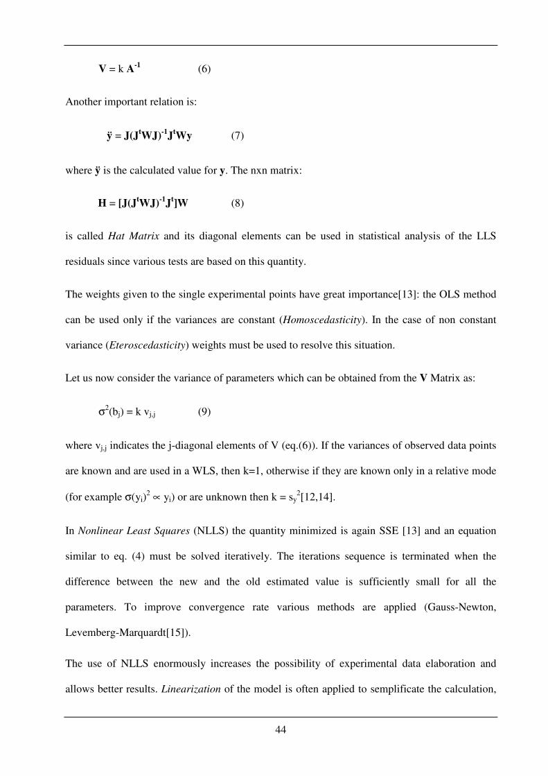
44

V = k A-1 (6)

Another important relation is:

ÿ = J(JtWJ)

-1J

tWy (7)

where ÿ is the calculated value for y. The nxn matrix:

H = [J(JtWJ)

-1J

t]W (8)

is called Hat Matrix and its diagonal elements can be used in statistical analysis of the LLS

residuals since various tests are based on this quantity.

The weights given to the single experimental points have great importance[13]: the OLS method

can be used only if the variances are constant (Homoscedasticity). In the case of non constant

variance (Eteroscedasticity) weights must be used to resolve this situation.

Let us now consider the variance of parameters which can be obtained from the V Matrix as:

σ2(bj) = k vj,j (9)

where vj,j indicates the j-diagonal elements of V (eq.(6)). If the variances of observed data points

are known and are used in a WLS, then k=1, otherwise if they are known only in a relative mode

(for example σ(yi)2 ∝ yi) or are unknown then k = sy

2[12,14].

In Nonlinear Least Squares (NLLS) the quantity minimized is again SSE [13] and an equation

similar to eq. (4) must be solved iteratively. The iterations sequence is terminated when the

difference between the new and the old estimated value is sufficiently small for all the

parameters. To improve convergence rate various methods are applied (Gauss-Newton,

Levemberg-Marquardt[15]).

The use of NLLS enormously increases the possibility of experimental data elaboration and

allows better results. Linearization of the model is often applied to semplificate the calculation,

45

but it is a bad pratique as it introduces biases in statistical weight of data[12,14]; in these cases

NLLS fitting is a better choice[10].

A critical point in nonlinear fits is the initial selection of parameter values. If the initial values

are far from the true ones, the calculation can diverge or converge to a local minimum[15].

Another great limit of NLLS is the estimation of the errors on parameters which is very

complex[16], but often good values can be obtained using eq (9) if n are large and the error

values are small[12].The errors obtained whit this way are called Asymptotic Errors. A Monte

Carlo Study (MC) can often validate the reliability of data treatment[1,17].

In spite of these problems, the use of NLLS displays great attractive for its simplicity to be set up

as a spreadsheet and for its direct connection between experimental data and theoretical model.

2.3.2.Statistical Evaluation of Fitting.

In this field E. J. Billo[18] proposed a pionieristic application in the evalutation of parameters

precision in NLLS with Excel. Some other authors presented the use of Excel with LLS and

NLLS[3,11,19] and some of them [8,20] used various methods to obtain error estimates of the

parameters but for an accurate and selective diagnostic an adequate statistical treatment of data

and result of fitting is of paramount importance.

In order to use Excel Solver for minimizing our experimental data, a column vector was written

in the worksheet with n cells for the value weights, one column (or more) for independent

variable(s), one for dependent variable, one for the appropriate formula to be applied to calculate

dependent variable and one for squared residuals. A cell which contains the sum of weighted

residuals was also inserted. In a row vector with p cells the initial estimate values of parameters

were reported.

46

Then Excel Solver was used and the minimized LLS or NLLS parameters obtained.

The statistical evaluation of the model is now crucial and this is provided by SolverStat, a

Routine based on well defined statistical tests[13,17,21], written in an Excel VBA (Visual Basic

for Application), a simple and powerful Excel programming language[22,23].

This routine analyzes: (a) the regression triplet[6], i.e. the data quality for a proposed model, the

model quality for a given data set, the regression method quality, that is the fulfilment of all LS

assumption and (b) can discriminate between different models allowing the selection of the best.

The routine calculates the corrispective statistic and when available the corrispective critical

value for selected probability and/or the computed probability.

2.3.2.a.Regression Triplet

Data quality

As far as linear parameter models are concerned the following useful statistics for observations

diagnostic are available in SolverStat and are based on residuals r (eq. (2)) and Hat Matrix of eq.

(8).

One of the main goals of the observation diagnostics[24] is the identification of the outliers

(points whose residuals are so large that they indicate that either the model or the response for

the respective data point are erroneous) and the influential points (the points which remarkably

affect the model parameters ). If an outlier is influential, it will cause serious distortions in the

regression calculations. Once an observation has been determined to be an outlier, it must be

checked to see if it resulted from a mistake. If so, it must be corrected or omitted. However, if no

mistake can be found, the outliers should not be discarded just because are outliers as they often

47

suggest that the model is inadequate. For a good review on outliers and influential points statistic

application in chemistry see refs. 5,6.

A first diagnostic test is based on the value of the hat diagonal hjj (leverage)[21]. Cut point for

this statistic is 2p/n or 3p/n. A high-leverage observation is not a bad observation but exerts extra

influence on the final results.

Studentized Deleted Residual (called also Jackknife Residuals)[24] is calculated by scaling the

residuals using a computed variance omitting a certain point, j, from the regression. The idea is

that, excluding this point, a better estimate of the variance will be obtained if the point is an

outlier. This statistic has a t distribution with (n – p – 1) degrees of freedom[5]. Other suggested

cutoff are values of 2 or 3[21].

A good diagnostic plot that helps in simultaneous visualization of outliers and influential point is

the Williams Graph[21] in which Studentized Deleted Residuals is plotted versus leverages

value.

DFFITS is the standardized difference between the predicted value with and without that

observation[24]. If the absolute value of DFFITS is larger then 1, the observation should be

considered to be influential . Suggested cut point for this statistic are p/n2 or p/n3 [21].

Another statistic test is the Cook’s Distance [24] which measures the influence of each point on

all fitted data. Values greater than one indicates a point that has large influence. Suggested

cutoff value was 1 or 4 / (n - 2) [21] or the 50th percentile of the F-distribution with (p, n – p)

DF[5].

The COVRATIO[13] describes the influence of each j point on the variance of estimated

parameters. A value exceeding 1 implies that the observation j provides an improvement in the

fitting quality; a value of CovRatio less than 1 flags an observation that decreases the precision

48

of the model. A suggested guideline is that if CovRatio > 1 + 3p / n then omitting this

observation significantly damages the precision of at least some of the regression estimates. If

CovRatio < 1 - 3p / n then omitting this observation the precision of at least some of the

regression estimates significantly improves.

The DFBETAS criterion measures the standardized change in a regression parameters when an

observation is omitted[24]. Common cutpoint was n2 or n3 . when n is greater than 100.

When n is less than 100, some authors have suggested to use a cut-off of 1 or 2 for the absolute

value of DFBETAS[21].

Model Quality

The first test applied is Model ANOVA (ANalysis Of the VAriance, an F-Test)[13] that gauges

the contribution of the independent variables in predicting the dependent variable. If the F ratio

is around 1, the model association between the variables described in the model are not

statistically significative.

If in the model fitted, the weights of the points are based on independently known variance, the

sum of weighted residual squared S in eq. (1) is tested with the Chi Square Statistic[17]. This

tests if the variance of the checked model is compatible with the true known variance. If this test

fails, the model is inadequate to describe the data or the known variance is not the true.

Runs-of-Sign Statistic test has also been introduced to evaluate if runs of identical signs in

residuals occur by chance[24]. The test fails when the calculated curve deviates systematically

from the data points: in that case the model is likely inadequate.

Parameters Error computation is based on eqs. (5), (6) and (9). As usual[12,13,21] a Student Test

t with n-p degree of freedom checks if the single parameter is statistically different from zero. If

49

the test is negative then the parameter is not significative to describe the model or the data

scattering of the points is too wide. In the case of use of independent known variance for data

point, SolverStat uses the Normal Statistic Z for this test[12].

Correlations between parameters are calculated from the matrix V:

)V (V /VR lmlmlmlmCorr = (10)

where subscripts l and m refer to different parameters. When the function parameters are

correlated, the Confidence Intervals (CI) calculated using the usual t statistic will be significantly

underestimated[16]. More reasonable values are the Joint Confidences Intervals (JCI) that can be

calculated using a F Statistic with (p, n-p) degrees of freedom. When independent known

variance is used this Statistic must be replaced with a χ2 Statistic with p degrees of freedom[16].

The errors and the confidence intervals calculated in this way, are corrected only for linear

parameters; for NLS CI can be more wide, sharp or asymetrics[16]. Nevertheless their reliability

is good if the relative standard error is better than 1/10[12].

An additional tool introduced in SolverStat, based on Monte Carlo Simulation[17], can be

invoked to check the correct goodness of parameters error in the nonlinear case. The limit of this

optional utility is that it takes a very long time to end the calculations (typically 0.1-1 second for

each single simulation).

The central idea behind MC[1,17,26-28] sampling is that the finite–sized data sets collected in

the laboratory are drawn from a distribution of possible experimental results (due to random

measurements errors). MC sampling allows a quantitative determination of precision by

generating a large number of data sets consistent with the experimentally measured data (i.e.

drawn from a normal distribution with the same mean observed in the laboratory and a standard

deviation equal to the error estimate for each data point). After carrying out the fitting procedure

50

on each member of the synthetic data set, a distribution of parameter values is obtained whose

standard deviations are the uncertainty in the fit parameters. MC simulation is one of the most

precise method for the evaluation of CI of determinated parameters[16]. For this purpose the

validity of the method is dependent on how realistically the set of pseudorandom uncertainties

models the uncertainties in the actual experimental data.

Regression Method Quality

Some conditions are to be observed for the applications of LS fit[13]: (i) absence of

multicollinearity (the presence of high or near-perfect intercorrelations between or among the

independent variables) in the case of multiple regression analysis (ii) residuals are normally

distributed; (iii) residuals have constant variance (Homoscedasticity); (iv) residuals are

independent from each other.

The problem of multicollinearity (i) is analyzed with the Variance Inflaction Factor (VIF), a test

based on the R2 obtained when each variable is regressed on the remaining independent

variables. Collinearity arises sfrom sampling methodology, over-defined model, model choice

and outliers. Multicollinearity determines inaccurate estimates of the regression parametes, alters

the result of varius tests and degrades the predictability of the model. A VIF of 10 or greater

indicates a multicollinearity problem[13].

Point (ii) is tested with Shapiro-Wilk Statistic SW (for large samples SolverStat uses a Shapiro-

Francia modification)[25]; if the calculated SW value is less than a selected critical value, the

residuals are not normally distributed and the model might not be adeguated. Another test is the

Jarque-Bera Statistic JB based on the coefficient of skewness and kurtosis. JB is distribuited as a

Chi Square Distribution χ2 with 2 DF: JB test is more useful with large data sets, SW is a better

choice with small data sets[25].

51

The Constant Variance of Residuals (iii) is examined with Levene F Test[13]: if calculated F

value is less than a critical value, residuals can be considered to have constant variance; if the

test fails, either the model chosen is inadequate or it is necessary to use non constant weighting

of the data. In this case a review of the background of model choice and of the experimental

procedure are essential.

Independence of residuals (iv) can be tested with Durbin-Watson Statistic DW[19] for first order

autocorrelations. The presence of autocorrelation arises from time sequenced data or model

misspecification and causes understimation of confidence intervals and distorsion of various

statistical tests. If the residuals are not correlated, the Durbin-Watson statistic will be around 2.

If violation of regression assumption are detected, it is necessary to take opportune corrective

action such as the delection of outliers for the violation of residuals normality or the use of WLS

for the case of Eteroscedasticity. See refs. 13 and 24 for more details.

2.3.2.b. Models Discrimination

When different models pass previous checks for regression triplet analysis, the comparison can

be performed by means of various statistical criteria. The classical, not fully satisfactory,

approach is based on the evaluation of the residuals and error magnitude on minimized

parameters and selecting the model with the lowest values. Other information can be obtained

from Multiple Correlation Coefficient R, Coefficient of Multiple Determination R2 and Adjusted

Coefficient of Multiple Determination R2adj [13]. This statistic evaluation indicates the fraction of

total variability in the data shown by the regression model. The R2adj is superior to the common

R2 value as it is sensitive to addition of irrelevant variables (R2adj decrease s whereas R2 increases

or at least stays constant).

52

When the differences within more models are low, SolverStat helps in the selection of the more

reliable one with two type of F-Test. The first is called Extra Sum of Squares F-Test, FExSS[13]

and is based on the ratio between the differences of SSE for the full model minus SSE for the

reduced model and SSE for the full model:

FExSS = (SFull - SReduced) / SFull DFFull / (DFFull - DFReduced) (11)

Only if FExSS is large, the addition of one or more terms to the reduced model significantly

improves the model.

The second available F-Test[21] ( F value for Models Comparison in Table 1) compares the SSE

of the two examined model and determine if the differences are statistically significative (S2 >

S1):

FRSS = (S2 / DF2) / (S1 / DF1) (12)

If calculated F is larger than selected critical value at desired confidence level, then the two

models are different and the model with low variance is really the best.

Another available decision tool is the Prediction Error Sum of Squares (PRESS)[21] a test based

on hjj. The smaller PRESS is, the better the predictability of the model.

The PRESS value can be used to compute the R2Prediction, which reflects the prediction ability of

the model. It is possible to have a high R2 and a low R2Prediction. In a similar way as R2

adj this

statistic shows a maximum for the best predictive model. The difference is that R2Prediction is

based on the predictive power of the model.

The last subset selection tool available is the Akaike Information Criteria (AIC)[24]. It is based

on measuring the fit given by SSE and correcting it for the number of regressors. The best model

will show low value of AIC.

53

2.3.3. Procedure for regression model building

The next procedure can therefore be used for the regression model building:

(vi) Proposal of a model from theory and preliminary exploration of data

(vii) Make the regression model

(viii) Run regression and statistic

(ix) Conduct the triplet analysis.

(d) If after examination of data quality, some outliers are found and deleted, go to (iii)

(e) If after examination of model quality some parameters are omitted go to (ii)

(f) if the examination of regression method evidences the necessity of corrective action,

take opportune remedial measures and go to (ii)

(x) If more than one model is selected and not discarded by the regression triplet, then

conduct a model discrimination.

References.

[1] S.E. Feller, C.F. Blaich, J. Chem. Educ. 76(11) (1999) 1594-1598.

[2] D.P. Shoemaker, C.W. Garland, J.W.Nibler, Experiments in Physical Chemistry, 5th ed.; Mc-

Graw-Hill: New York, 1989.

[3] M. Iannone, J.Chem,.Educ. 75(9) (1998) 1188-1189.

[4]. M.Meloun, M.Pluhařová, Anal. Chim. Acta 416 (2000) 55-68.

54

[5] M.Meloun, J.Militky, Anal.Chim.Acta 439 (2001) 169-191.

[6]M.Meloun, J.Militky, K. Kupka, R.G. Brereton, Talanta 27 (2002) 721-740 and refs. therein.

[7] P.Gans, A.Sabatini, A.Vacca, Talanta 43 (1996) 1739-1753 and refs. therein.

[8] P. Kuzmič, Anal. Biochem. 237 (1996) 260-273; Anal. Biochem. 267 (1999) 17-23.

[9] R. de Levie, J.Chem.Educ. 76(11) (1999) 1594-1598.

[10] T.J. Zielinsky, R.D. Allendoerfer, J.Chem.Educ. 74(8) (1997) 1001-1007.

[11] P. Denton, J.Chem.Educ. 77(11) (2000) 1524-1525.

[12] J. Tellinghuisen, J.Phys. Chem. A 104(12) (2000) 2834-2844.

[13] J.Neter, M.H .Kutner, C.J. Nachtsheim, W. Wasserman, Applied Linear Regression Models, 3th

ed.; Irwin: Chicago, 1996.

[14] J. Tellinghuisen, J.Phys. Chem. A 104(50) (2000) 11829-11835.

[15] J.O. Machuca-Herrera, J.Chem.Educ. 74(4) (1997) 448-449.

[16] a) L. M. Schwartz, Anal. Chim Acta 122 (1980) 291-301. b) M.L. Johnson,

Biophis. J. 44(10) (1983) 101-106. c) M.L. Johnson, Anal.Biochem. 206 (1992) 215-

225. d) M.L. Johnson, L.M. Faunt, Methods Enzymol. 210 (1992) 1-37. e) D.G, Watts,

Methods Enzymol. 240 (1994) 23-36.

[17] W.H. Press, B.P. Flannery, S.A.Teukolsky, W.T. Vetterling, Numerical Recipes,

Cambridge University Press: New York, 1989.

[18] E.J. Billo, “Excel for Chemists, A Comprehensive Guide, Wiley-VCH, New York,

1997.

[19] E. Howard, J. Cassidy, J.Chem.Educ 77(3) (2000) 409-411.

55

[20] D.C. Harris, J.Chem.Educ. 75(1) (1998) 119-121.

[21] R. Todeschini, Introduzione alla Chemiometria, Edises: Napoli, 1998

[22] J.Walkenbach, Excel 97 Programming For Windows For Dummies, IDG Books

Worldwide, 1997

[23] R. De Levie, Excel in Analytical Chemistry, University Press, Cambridge, 2001.

[24] T.P. Ryan, Modern Regression Methods Wiley Eds., N.Y., 1997

[25] J.M. Dufour, A. Farhat, L.Gardiol, L.khalaf, Econometrics J. 1 (1998) 154-173.

[26] P. Ogren, B. Davis, N. Guy, J.Chem.Educ. 78(6) (2001) 827-836.

[27] J.S. Alper, R.I. Gelb, J.Phys.Chem. 94(11) (1990) 4747-4751.

[28] R.M.C. Goncalves, F.E.L. Martins, R.A.E. Leitao, 98(38) (1994) 9537-9540.

56

9 LOGISTIC REGRESSION ANALYSIS[1]

Often we wish to evaluate the effects of multiple explanatory variables on a binary outcome

variable. For example, the effects of a number of risk factors on the development or otherwise of

a disease. A patient may be cured of a disease or not; a risk factor may be present or not; a

person may be immunised or not, and so on. The situation is different from multiple regression

analysis which requires that the outcome variable be measured on a continuous scale. When the

outcome variable is binary, and one wishes to measure the effects of several independent

variables on it the method of analysis to use is Logistic Regression. The binary outcome variable

is coded 0 and l. The convention is to associate 1 with 'success' (e.g. patient survived; risk factor

is present; correct answer is given, and so on), and 0 with 'failure'.

For Logistic Regression the following conditions need to be satisfied:

1) An outcome variable with the two possible categorical outcomes, preferably in the form 0

and 1. (A dummy variable may have to be created for the purpose).

2) We need to estimate the probability P of the observed value of the outcome variable out

of 1.

3) We need a way of relating the outcome variable to the explanatory variables. This is done by

means of the logistic function, which is explained later.

4) We need a way of estimating the coefficients of the regression equation developed.

5) We need to test the goodness of fit of the regression model, as well as estimate the

confidence intervals of the coefficients.

Logistic regression can be used only with two types of target variables:

1. A categorical target variable that has exactly two categories (i.e., a binary or dichotomous

variable).

2. A continuous target variable that has values in the range 0.0 to 1.0 representing probability

values or proportions.

Recall that in multiple linear regression the basic activity is to draw the least square line around

which the values of Y (the outcome variable) are distributed. In contrast to that, in logistic

regression we are trying to estimate the probability that a given individual will fall into one

outcome group or the other. Thinking in terms of probability helps to interpret the coefficients in

the logistic regression model in a meaningful manner, in the same way as we attach meaning to

the coefficients in linear regression.

57

As a measure of the probability we ask about the odds of an event occurring. If P is the

probability of a given event, then (1 - P) is the probability of the event not occurring. The odds of

the event can be defined as:

Probability of event occurring -r- Probability of event not occurring.

In other words, P / (1 - P) is the ratio of the probability of success, also called the odds of

success. (When given the odds ratio, we can calculate probability from P = odds ratio -r- (1 +

odds ratio).

If there are several factors involved in deciding the eventual outcome we can calculate the odds

ratio for each one separately. (This kind of crude odds ratio was described in relation to case -

control studies in Chapter 6 of Mother and Child Health: Research methods). The joint effect of

all the independent variables put together may be expressed mathematically as:

Odds = P / (1 - P) = e α + β1 X1 + β2X2 + ... + βp Xp

Where e is a mathematical expression (like n). The numerical value of e is equal to 2.71828.

The independent contribution of each of several factors (i.e. X1, X2 ... Xp) in the above

expression to the overall odds ratio can be determined by taking the logarithms of both sides of

the equation.

Loge{P / (1-P)} = loge {e α + β1 X1 + β2X2 + ... + βp Xp}

The term log {P / (1-P)} is referred to as 'logistic transformation of the probability P, and is

written as logit (p), which is short for 'logistic unit'. Transforming the counted proportion p (so

many successes out of so many trials) to logit gets rid of the drawback of probability which

varies from 0 to 1, whereas the logit can vary from -x to + x. And so we have now natural

logarithm of (P / 1- P) = logit P = β0 + β1 X1 + ... + βp Xp

The right hand side of the equation is the same as in multiple linear regression with which we are

familiar. Recall that in linear regression the parameters of the model are estimated using the least

squares approach. What happens is that the coefficients selected are such that the sums of

squared distances between the observed values and the predicted values (i.e. the regression line)

are smallest.

In logistic regression the parameters are estimated such that the coefficients make our observed

results most likely. The method is called the maximum likelihood method. What does it all mean?

Suppose in the above equation the two possible values of the outcome variable are presence or

absence of disease, (with presence of disease =1). Then a represents the overall disease risk,

while P1 is the fraction by which the risk is increased (or decreased) by every unit change in X1;

p2 is the fraction by which the disease risk is altered by a unit change in X2, and so on. The

independent variables can be quantitative or qualitative e.g. by using dummy variables.

However, one should bear in mind that the logit of a proportion p is the logarithm of the

corresponding odds. If an X variable has a coefficient P, then a unit increase in X increases the

log odds by an amount equal to P. This means that the odds themselves are increased by a factor

58

of eP. So if P = 1.6, the odds are e1.6 = 4.95 .The logarithms of all the odds can be converted back

to probability by the formula P = ey/(1+ey).

References

[1] Journal of Tropical Pediatrics. Research Methods II. Chapter 11: Logistic regression.

http://www.oxfordjournals.org/our_journals/tropej/online/ma_chap11.pdf (Accessed August,

2010).

59

10 POISSON REGRESSION ANALYSIS[1]

In clinical work one often encounters situations where the outcome variable is numeric, but in

the form of counts. Often it is a count of rare events such as the number of new cases of lung

cancer occurring in a population over a certain period of time. The aim of regression analysis in

such instances is to model the dependent variable Y as the estimate of outcome using some or all

of the explanatory variables (in mathematical terminology estimating the outcome as a function

of some explanatory variables.

When the response variable had a Normal distribution we found that its mean could be linked to

a set of explanatory variables using a linear function like

Y = β0 + β1 X1 + β2 X2 + ... + βk Xk

In the case of binary regression the fact that probability lies between 0-1 imposes a constraint.

The normality assumption of multiple linear regression is lost, and so also is the assumption of

constant variance. Without these assumptions the F and t tests have no basis. The solution was to

use the logistic transformation of the probability p or logit p, such that

loge(p/(1- p)) = β0 + β1 X1 + β2 X2 + ... + βn Xn

The p coefficients could now be interpreted as increasing or decreasing the log odds of an event,

and expp (the odds multiplier) could be used as the odds ratio for a unit increase or decrease in

the explanatory variable. In survival analysis we used the natural logarithm of the hazard ratio,

that is:

loge h(t)/h0 (t) = β0 + β1 X1 + ... + βn Xn

When the response variable is in the form of a count we face a yet different constraint. Counts

are all positive integers and for rare events the Poisson distribution (rather than the Normal) is

more appropriate since the Poisson mean > 0. So the logarithm of the response variable is linked

to a linear function of explanatory variables such that:

loge (Y) = β0 + β1 X1 + β2 X2 ...

and so

Y = (e β0) (e β1X1) (e β2X2) .. etc.

In other words, the typical Poisson regression model expresses the log outcome rate as a linear

function of a set of predictors.

10.1 ASSUMPTIONS IN POISSON REGRESSION

The assumptions include:

60

1) Logarithm of the disease rate changes linearly with equal increment increases in the exposure

variable.

2) Changes in the rate from combined effects of different exposures or risk factors are

multiplicative.

3) At each level of the covariates the number of cases has variance equal to the mean.

4) Observations are independent.

Methods to identify violations of assumption (3) i.e. to determine whether variances are too large

or too small include plots of residuals versus the mean at different levels of the predictor

variable. Recall that in the case of normal linear regression, diagnostics of the model used plots

of residuals against fits (fitted values). This means that the same diagnostics can be used in the

case of Poisson Regression.

References

[1] Journal of Tropical Pediatrics. Research Methods II. Chapter 13: Poisson regression analysis.

http://www.oxfordjournals.org/our_journals/tropej/online/ma_chap13.pdf (Accessed August,

2010)

61

11 PRINCIPAL COMPONENT ANALYSIS [1]

A principal component analysis (PCA) is concerned with explaining the variance-covariance

structure of a set of variables through a few linear combinations of these variables, called

principal components. Its general objectives are:

• Data reduction

• Interpretation

In general, p principal components are required to reproduce the total system of variability of the

original data set (n measurements on p variables). Fortunately, much of this variability can often

be accounted for by a small number of k of principal components. If so, there is (almost) as much

information in the first k components as there is in the original p variables.

The k first principal components can then replace the initial p variables, and the original n x p

data set is reduced to n x k data set consisting of n measurements on k principal components.

An analysis of principal components often reveals relationships that were not previously

suspected and thereby allows interpretations that would not ordinarily result.

Principal components also frequently serve as intermediate steps in much larger investigations,

e.g. as inputs to a multiple regression, cluster analysis, etc.

References

[1] Rovan, J. Multivariate Analysis. Chapter 9: Principal Component Analysis.

http://miha.ef.uni-lj.si/_dokumenti3plus2/193004/MVA_06_Principal_Component_Analysis.pdf

(Accessed August, 2010).

62

12 OTHER SUGGESTED SOFTWARE & LINKS:

Statistics:

R - http://cran.r-project.org/

PAST - http://folk.uio.no/ohammer/past/

GRETL - http://gretl.sourceforge.net/

TANAGRA - http://eric.univ-lyon2.fr/~ricco/tanagra/index.html

Bayesian:

WINBUGS - http://www.mrc-bsu.cam.ac.uk/bugs/winbugs/contents.shtml

OPENBUGS - http://www.openbugs.info

SMILE and GENIE - http://genie.sis.pitt.edu/

Numerical and algorithms:

http://digilander.libero.it/foxes/

http://lib.stat.cmu.edu/apstat/

http://jblevins.org/mirror/amiller/

solverstat: the manual - webs

Documents