Solving an integrated employee timetabling and job-shop

scheduling problem via hybrid branch-and-bound

Christian Artigues1, Michel Gendreau2, Louis-Martin Rousseau2 and Adrien Vergnaud2

1LAAS–CNRS

7 avenue du Colonel Roche, 31077 Toulouse, France

christian.artigues@laas.fr2CRT – Universite de Montreal

C.P. 6128, succursale Centre-ville, Montreal, QC H3C 3J7 Canada{michelg,louism}@crt.umontreal.ca

Abstract

We propose exact hybrid methods based on integer linear programming and constraintprogramming for an integrated employee timetabling and job-shop scheduling problem. Eachmethod we investigate uses a constraint programming (CP) formulation associated with alinear programming (LP) relaxation. Under a CP framework, the LP-relaxation is integratedinto a global constraint using in addition reduced cost-based filtering techniques. We proposetwo CP formulations of the problem yielding two different LP relaxations. The first formula-tion is based on a direct representation of the problem. The second formulation is based on adecomposition in intervals of the intervals of the possible operation starting times. We showthe theoretical interest of the decomposition-based representation compared to the directrepresentation through the analysis of dominant schedules. Computational experiments ona set of randomly generated instances confirms the superiority of the decomposition-basedrepresentation. In both cases, the hybrid methods outperforms pure constraint program-ming for employee cost minimization while it is not the case for makespan minimization.The experiments also investigate the interest of the proposed integrated method comparedto a sequential approach and show its potential for multiobjective optimization

1 Introduction

In production systems, the decisions related to scheduling jobs on the machines and the decisionsrelated to employee timetabling are often made in a sequential process. The objective of jobscheduling is to minimize the production costs whereas the objective of employee timetabling isto maximize employee satisfaction (or to minimize labor costs). Either the employee timetablingis first established and then the scheduling of jobs must take employee availability constraintsinto account or the scheduling of jobs is done at first and the employees must then adapt to coverthe machine loads. It is well known that optimizing efficiently an integrated process would allowto balance production costs and employee satisfaction in a better way. However, the resultingproblem has generally been considered as too complex to be used in practical situations. Someattempts have been made [DM94, BAL95, DHM96, AB97, Che04, HCM04, DMS04] but mostlyconsidering an oversimplified version of the employee timetabling problem. Nevertheless the inte-gration of task scheduling and employee timetabling has been successfully developed in complextransportation systems [BGAB83, DDI+98, HF99, CSSD01, KJN02, FHW03, MCS05]. In thecontext of production or project scheduling, even basic integration processes, considering man-power availability in an aggregated way, have shown however substantial cost savings [BAL95].

1

There is consequently a potential on developing models that consider detailed timetabling ofindividual employees as well as detailed scheduling of job operations on machines.

In the classical employee timetabling problem [EJKS04, DPR05], the employee horizon isdecomposed in shifts and the employee timetabling problem aims at assigning to each employee asingle activity during each shift while minimizing the employee cost, each employee having skillsfor a limited number of activities. The classical job-shop scheduling problem [BDP96] considers aset of jobs and a set of machines. Each job is a chain of operations, each operation being definedby its duration and its assigned machine. The job-shop scheduling problem aims at assigninga start time to each operation such that the precedence constraints between the operations ofthe same job are satisfied and such that the processing intervals of any two operations assignedto the same machine do not overlap. The job-shop scheduling objective is to minimize themakespan. Integrating employee timetabling and job-shop scheduling has to be performed bydefining how the employee activity demand is determined by the schedule of job operations onthe machines.

In [DMS04], the assumption is made that each job operation has to be performed by itsmachine, plus a set of employees assigned to the operation during its entire processing time.This amounts to consider employees as additional parallel machines, each machine being ableto process only a subset of operations because of limited employee skills. However in practice,the decomposition in shifts of the employee timetabling horizon leads to the case where theset of employees assigned to the operation can be modified while the operation is in process,generally at a shift change. Drezet and Billaut [DB06] propose a more complex model, in thecontext of resource-constrained project scheduling, taking account of this characteristic, amongothers. In [HBBF05], Haıt et al. propose a general model for integrated production schedul-ing and employee timetabling, based on the concepts of load center, configuration, employeeassignment and sequence. A so-called load center is a subset of machines that can be managedsimultaneously by a single employee. A configuration is a set of load centers defining a partitionof a subset of machines. At each scheduling time period, a single configuration can be active.Hence, the number of load centers in a configuration gives the number of active employees. Anemployee assignment is an assignment of each load center of a configuration to a different em-ployee. The authors define the configuration graph in which each node corresponds to a possibleconfiguration and there is an arc between two configurations that can be consecutive in timewith a weight giving the cost of the configuration changeover. This model emphasizes that inproduction systems employee activities are more associated with machine than with operations.Furthermore, it allows to represent the simultaneous work of an employee on several machines,e.g. for supervision activities.

In this paper we propose a simple model making a synthesis of the previously defined models,in the context of a job-shop. This model basically links the employee activity to the resource us-age during the employee shift, while the required skills are determined by the operations actuallyscheduled on the machine during this shift. The model allows also an employee to work simulta-neously on several machines. We consider further flexibility in the operation schedule/activitydemand mapping by allowing an employee shift to cover more than one scheduling period, ag-gregating the demand of the operations scheduled during the shift. We consider a lexicographicoptimization problem where the makespan minimization is the primary objective whereas theemployee cost minimization is the secondary objective. The problem is presented in Section 2.

The integration of two NP-hard optimization problems is unlikely to give an easily solvableproblem. On one hand, the vast literature on job-shop scheduling shows that exact makespanminimization methods are based on efficient constraint propagation techniques [BPN01]. Onthe other hand, employee cost minimization methods, especially in the airline crew schedulingproblems, are often based on integer linear programming methods [EJKS04]. It follows that

2

the integrated employee timetabling and job-shop scheduling problem appears as a potentialapplication of hybrid methods, incorporating elements from both constraint programming (CP)and integer linear programming (ILP) as already successfully developed for other integratedplanning and scheduling problems [FLN00, Hoo05]. The exact hybrid methods we investigateuse a CP formulation associated with a linear programming (LP) relaxation. The LP relaxationis integrated into a global constraint using reduced cost-based filtering [FLM99]. We proposetwo CP formulations of the problem yielding two different LP relaxations. The first formulation,described in Section 3, is based on a direct representation of the problem. The second formula-tion, given in Section 4, is based on a decomposition in intervals of the set of possible operationstart time values. We show in Section 5 the theoretical interest of the decomposition-basedrepresentation compared the direct representation through the analysis of dominant schedules.Computational experiments on a set of randomly generated instances are given in Section 6.Concluding remarks are drawn in Section 7.

2 A flexible model for integrated employee timetabling and job-

shop scheduling

We consider a set of machines {Mk}k=1,...,m and a set of jobs {Ji}i=1,...,n, each job Ji being madeof a chain of operations {Oij}j=1,...,m. Each operation Oij is defined by its assigned machinemij ∈ {M1, . . . ,Mm} and its duration pij > 0. All durations are assumed to be integers. Theset of operations assigned to machine Mk is denoted Ok. H denotes the scheduling horizon, anupper bound of the schedule completion time.

We also consider a set of employees {Ee}e=1,...,µ, a set of activities {Aa}a=1,...,α and a set ofshifts {s}s=0,...,σ−1. All shifts s are assumed to have the same duration π ≥ 1. The timetablinghorizon σ is defined such that H = σ × π. The cost of assigning employee Ee to activity Aa

during shift s is denoted ceas. Ae denotes the set of activities an employee is able to perform.We assume there is an additional activity A0 representing employee inactivity and such thatA0 ∈ Ae for each employee Ee. Employee Ee is assumed to be available for a subset of shiftsTe. Each operation Oij is assumed to require during its processing an integer number bija ≥ 0employees for activity a.

Solving the problem lies in assigning values to the following decision variables. Sij denotesthe start time of operation Oij . Cij denotes the completion time of operation Oij . Cmax denotesthe makespan of the schedule. xeas is a binary variable equal to 1 if employee Ee is assigned toactivity a during shift s. θijs is a binary variable equal to 1 if operation Oij is in process duringshift s. δas is the number of employees required for activity a during shift s (demand). Theproblem can be formulated as follows, mixing for convenience linear and logic formulations.

• Objective function:

minLex

(

Cmax,

µ∑

e=1

α∑

a=1

σ−1∑

s=0

ceasxeas

)

(1)

• Job-shop specific constraints:

Cmax ≥ Cim i = 1, . . . , n (2)

Cij = Sij + pij i = 1, . . . , n j = 1, . . . ,m (3)

Sij ≥ Ci(j−1) i = 1, . . . , n j = 2, . . . ,m (4)

(Sij ≥ Ckl) ∨ (Skl ≥ Cij) Oij 6= Okl,mij = mkl (5)

Sij ≥ 0 i = 1, . . . , n j = 1, . . . ,m (6)

3

• Employee timetabling specific constraints:

µ∑

e=1

xeas ≥ δas a = 1, . . . , α s = 0, . . . , σ − 1 (7)

∑

a∈Ae

xeas = 1 e = 1, . . . , µ s = 0, . . . , σ − 1 (8)

xe0s + xe0(s+1) + xe0(s+2) ≥ 2 s = 0, . . . , σ − 4 (9)

σ−1∑

s=0

xeas = 0 e = 1, . . . , µ a 6∈ Ae (10)

xe0s = 1 e = 1, . . . , µ s 6∈ Te (11)

xeas ∈ {0, 1} e = 1, . . . , µ a = 0, . . . α s = 0, . . . , σ − 1 (12)

• Coupling constraints:

Sij < (s + 1)π ∧ Cij > sπ =⇒ θijs = 1 i = 1, . . . , n j = 1, . . . ,m

s = 0, . . . , σ − 1 (13)

Sij ≥ (s + 1)π ∨ Cij ≤ sπ =⇒ θijs = 0 i = 1, . . . , n j = 1, . . . ,m

s = 0, . . . , σ − 1 (14)

δas =

m∑

k=1

maxOij∈Ok

θijsbija a = 1, . . . , α s = 0, . . . , σ − 1 (15)

For the job shop part, constraints (2) defines the makespan. Constraints (3) link the start and thecompletion time of each operation. Constraints (4) state that each operation cannot start beforethe completion of its job predecessor. Constraints (5) are the so-called disjunctive constraintspreventing two activities assigned to the same machine from being processed in parallel. Eachdisjunctive constraint is non linear.

For the employee timetabling part, fully linear, constraints (7) are the standard demand coverconstraints for each activity and each shift. Constraints (8) state that each employee has to beassigned exactly one activity (including “rest” activity A0) during each shift. Constraints (9) areregulation constraints that state that each employee can work at most 1 shift during each glidingwindow of 3 shifts. Note that other more complex (and possibly non linear) regulation constraintscould be necessary for practical applications. Constraints (10) fix assignment variables to 0 dueto employee skills. Constraints (11) fix assignment variables to activity A0 because of employeeunavailability during some shifts.

The coupling part describes how operation schedule S and activity demand δ are linked.Constraint (13) and (14) set binary variable θijs to 1 if the processing interval of operation Oij ,equal to [Sij, Cij [, intersects shift s interval equal to [sπ, (s + 1)π[, and to 0 otherwise. It isassumed that the employee assigned to an activity Aa distinct from A0 during his shift is alsoassigned to a machine and has to perform only activity Aa on this particular machine duringthis shift. Therefore, suppose two operations Oij and Okl are in process during a shift s andrequire each one employee for the same activity Aa. In this case, two employees able to performAa are required during shift s if Oij and Okl are assigned to different machines while only oneemployee is needed if mij = mkl. Constraints (15) compute the demand δas for each activityand each shift, summing up the demands on each machine for the same shift. The machinedemand on a shift for an activity is equal to the highest demand of operations in process duringthis shift.

4

Let us consider a small example (the EJS1 instance) comprising 6 jobs, 4 machines, 4 ac-tivities 15 employees and 6 shifts. Shift duration is π = 8. Hence the scheduling horizon isH = 48. In Table 1 the job data (machines and durations) is provided. The durations havebeen randomly generated between 1 and 10. For the operations requests for activities (valuesbija) we consider the special case where operations require a single employee and where there isa mapping between activities and machines. Therefore, we have bijmj

= 1 and bija = 0, for alla 6= mij.

—————————————————–INSERT TABLE 1 ABOUT HERE

—————————————————–

Employee data is displayed in Table 2. Each row corresponds to an activity the employeeis able to perform. The assignment costs of the employee for this activity are displayed forall shifts. They have been randomly generated between 1 and 5 assuming they correspond toemployee preferences.

—————————————————–INSERT TABLE 2 ABOUT HERE

—————————————————–

An optimal solution of the problem is displayed in Figure 1. On top of the Figure, a Ganttdiagram displays the start times of the operations. At the bottom, the employee timetable isdisplayed, giving, for each employee and each shift, the activity (machine) performed and thecorresponding cost. A makespan of 45 is obtained with a total cost equal to 29. In this simpleexample, an employee is necessary on a machine for a shift whenever the processing interval ofan operation assigned to the machine intersects the shifts. We see that only shifts 0, 2 and 5require less than 4 employees thanks to the idleness of machines 4, 3 and 4, respectively.

—————————————————–INSERT FIGURE 1 ABOUT HERE

—————————————————–

3 Direct CP formulation and LP relaxation

The job-shop scheduling part of the problem (2-6) can be modeled easily through a constraint-based scheduling library such as ILOG scheduler. The operations and the machines they requireare declared as high level objects having internal decision variables. Each operation Oij has aduration Oij .p, a start variable Oij .S with domain {0, . . . ,H − Oij .p} and a completion vari-able Oij .C verifying Oij .C = Oij .S + Oij .p. Each machine Mk is declared as a unary resource,i.e. a discrete resource with availability 1. The Makespan Cmax is a variable with domain{0, . . . ,H}. Two types of constraints are defined on operations and machines. Binary temporalconstraints are used to model the precedence constraints (4) between operations. Disjunctiveresource constraints representing constraints (5) are defined on each machine Mk. In ConstraintProgramming, constraints can be expressed in a very general way through so-called global con-straints (such as the disjunctive constraint), with the counterpart that ad-hoc constraint propa-gation algorithms have to be defined for each global constraint. Efficient constraint propagationalgorithms exist for both precedence and disjunctive constraints. The temporal constraint prop-agation, disjunctive resource constraint propagation and edge-finding algorithms allow to reduce

5

the domains of start and completion variables during the search process. The start (comple-tion) time domain of an operation is denoted {ESi, . . . , LSi} ({ECi, . . . , LCi}). We refer to[BP96, BPN01] for more details on the filtering algorithms associated with constraint-basedjob-shop scheduling.

The employee timetabling part (7-12) can also be modeled in terms of constraint program-ming. The model involves an assignment variable Aes with domain Ae if s ∈ Ts and {A0}otherwise, associated with each employee Ee and each shift s. Variable Aes is equivalent to the0-1 variable xeas used in (7-12). We have indeed the following relation Aes =

∑αa=1 a · xeas.

A demand variable δas with domain {0, . . . , µ} is defined for each activity and each shift. Werepresent the timetabling problem with global constraints element, distribute and sequence

as performed in previous work, see e.g. [DPR05].The coupling part involves an additional demand variable δijas for each operation Oij , each

activity Aa and each shift s with domain {0, . . . , bija}.Given the above defined operations, machines and decision variables, the considered CP

formulation can be stated as the following constraint optimization problem.

minLex

(

Cmax,

µ∑

e=1

σ−1∑

s=0

ceAess

)

(16)

Oim.C � Cmax i = 1, . . . , n (17)

Oij .C � Oi(j+1).S i = 1, . . . , n j = 1, . . . ,m − 1(18)

Oij.require(Mk) k = 1, . . . ,m Oij ∈ Ok (19)

distribute((δas)a=1,...,α, (Aa)a=1,...,α, (Aes)e=1,...,µ) s = 0, . . . σ − 1 (20)

sequence((Aes)s=0,...,σ−1, {A0}, 3, 2, 2}) e = 1, . . . , µ (21)

Oij .S < (s + 1)π ∧ Oij .C > sπ =⇒α∧

a=1(δijas = bija) i = 1, . . . , n j = 1, . . . ,m

s = 0, . . . σ − 1 (22)

Oij.S ≥ (s + 1)π ∨ Oij .C ≤ sπ =⇒α∧

a=1(δijas = 0) i = 1, . . . , n j = 1, . . . ,m

s = 0, . . . σ − 1 (23)

δas =

m∑

k=1

maxOij∈Ok

δijas a = 1, . . . , α s = 0, . . . , σ − 1(24)

The objective function is the lexicographic minimization of the makespan and the employeetotal cost. The total cost is expressed as an element constraints as the decision variable Aes isused as an index in ceAess which is in CP the standard way of expressing a cost associated to adiscrete decision variable [TO02]. Constraints (17) and (18) are the binary temporal constraintsinvolved in the job-shop sub-problem. Constraints (19) are the disjunctive constraints. Con-straints (20) represent demand satisfaction through the global cardinality constraint distribute[Reg96] which states that for a given shift s and for each activity Aa exactly δas variables musthave value Aa in the activity assignment vector (Aes)e∈E of employees during period s. Con-straints (21) represent regulation constraints (9) by means of the sequence constraint [BC94]which states that in each sub-sequence of q variables of the sequence (Aes)s=0,...,σ−1, at most 2and at least 2 variables must have the value A0. Note that this constraint could be alternativelyrepresented by constraint regular which would be also suitable to represent more complex regu-lation rules [Pes04, DPR05, vPRS06]. Constraints (22-24) are a direct transcription of couplingconstraints (13-15) using demand variable δijas instead of binary variable θijs.

6

The CP model is solved by a backtrack search on the variable values after transforming theoptimization problem into a series of decision (satisfaction) problems. The lexicographic mini-mization problem is solved by first finding the minimum makespan through binary search. Themakespan is then fixed to its minimal feasible value and a second binary search is performed tominimize the total employee cost. At each node of the involved search trees, constraint prop-agation algorithms are used to detect inconsistencies and reduce the domains of the variables.As previously stated, each predefined global constraint is associated with a specific constraintpropagation algorithm.

In addition, we propose to integrate a LP relaxation of the model. The considered LPrelaxation is reduced to the timetabling problem with variables xaes. It is precisely the LPrelaxation of the ILP min

∑µe=1

∑αa=1

∑σ−1s=0 ceasxeas subject to (7 − 12), except that variable

δas is replaced by the smallest value in its current domain in the demand cover constraint (7).Variables xeas are preprocessed by analyzing the current domain of variable Aes: each variablexeas such that a 6∈ Aes is set to 0 and each variable xeas such that Aes = {Aa} is set to 1.

The resolution of the LP relaxation is embedded into the constraint propagation algorithmof a global constraint demandCover. During search, the constraint propagation algorithm ofdemandCover is called each time the lower bound of any variable δas is changed, which corre-sponds to a modification of the demand cover constraint, or when the domain of any assignmentvariable Aes is modified, which corresponds to fixing some variables xaes. Different rules forpropagation of the demandCover constraint are investigated in Section 6.

For the makespan minimization phase, each time the LP is unfeasible, demandCover failsand the current node can be pruned. For the total employee cost minimization phase, furtherreductions can be performed with reduced-cost based variable fixing techniques [FLM99]. Be-sides infeasibility, demandCover also fails if the optimal cost of the LP relaxation is not lowerthan the current upper bound Z of the total cost value (set by the binary search). If the LPis feasible then let Ceas denote the reduced cost of an activity assignment variable xeas and letTC∗ denote the current optimal LP solution value. The reduced-cost based domain reductiontechnique states that if TC∗ + Ceas > Z then activity Aa can be removed from the domain ofAes.

4 Decomposition-based CP formulation and LP relaxation

The CP formulation and the LP relaxation defined in the previous Section have the drawbackthat the job-shop scheduling part of the problem is absent of the LP relaxation. In this Section,we propose a second formulation based on a decomposition of the domains of the operationstart time variables into disjoint intervals such that the selection of an interval for an operationdetermines its demand for each activity on all the employee shifts.

When an operation Oij starts at time t it intersects all shifts s such that (s + 1)π > t andsπ < t + pij. This allows to compute for each time point t ∈ {ESi, . . . , LSi} the demand profileδijas(t) for each activity a and each shift s. Then all (consecutive) time points t1, t2 ∈ {ESi, LSi}such that δijas(t1) = δijas(t2) for all shifts s = 0, . . . , σ−1 can be grouped into the same demandinterval. With this process, the domain of the start time of each operation Oij can be partitionedinto consecutive demand intervals I1, I2, . . . , Ivij

. Each interval Iq corresponds to a demand bijqas

for each activity a and each shift s. Demand interval Iq comprises values {ESijq, . . . , LSijq} suchthat LSijq + 1 = ESij(q+1) for 1 ≤ q < vij, ESij = ESij1 and LSij = LSijvij

. Note that thenumber of demand intervals vij cannot exceed 2σ + 1 where σ is the number of shifts.

An illustrative example is displayed in Figure 2 where the start time domain of an operationis partitioned into 5 intervals. The demand profiles of the operation for each interval and for anactivity a such that bija = 1 are displayed at the bottom of the Figure.

7

—————————————————–INSERT FIGURE 2 ABOUT HERE

—————————————————–

We modify the constraint programming model presented in the preceding Section by intro-ducing a decision variable Iij for each operation Oij with domain {I1, . . . , Ivij

}. The job-shopscheduling and employee timetabling part of the CP model (16-21) do not change but the fol-lowing constraints (comprising element constraints) are added to enforce the correspondencebetween the start times and the demand intervals

Oij .S � ESijIiji = 1 . . . , n j = 1 . . . ,m (25)

Oij .S � LSijIiji = 1 . . . , n j = 1 . . . ,m (26)

Furthermore the coupling constraints (22-23) are replaced by the following constraints, alsocomprising element constraints:

δijas = bijIijas i = 1 . . . , n j = 1 . . . ,m a = 1, . . . , α (27)

Constraint (24) is left unchanged.Besides the simplification of the coupling constraints, this new model allows to introduce

the scheduling part in the LP relaxation by defining a new binary variable yijq equal to 1 if Oij

is assigned to demand interval Iq and to 0 otherwise. The variable corresponds to the discretevariable Iij . Hence the new variables are preprocessed as follows. Each variable yijq such thatIq 6∈ Iij is set to 0 and each variable yijq such that Iij = {Iq} is set to 1. A continuous demandvariable dask giving the demand for activity Aa on shift s issued from machine Mk is defined asan intermediate variable.

The model comprises constraints (8-12). The cover constraint (7) is removed and replacedby the following constraints:

vij∑

q=1

yijq = 1 i = 1, . . . , n j = 1, . . . ,m (28)

dask ≥

vij∑

q=1

yijqbijqas a = 1, . . . , α s = 0, . . . , σ − 1 k = 1, . . . ,m Oij ∈ Ok (29)

µ∑

e=1

xeas ≥m∑

k=1

dask a = 1, . . . , α s = 0, . . . , σ − 1 (30)

yijq ∈ {0.1} i = 1, . . . , n j = 1, . . . ,m q = 1, . . . , vij (31)

Constraints (28) state that only one interval has to be selected for each operation. Constraints(29) states that demand dask of machine Mk for activity Aa on shift s is not lower than thedemand for activity Aa on shift s of each operation Oij assigned to machine k, which is set bythe assigned interval. Constraints (30) enforce the employees assigned to activity Aa on shift s

to cover the total demand obtained by summing up all machine demands.In addition, scheduling constraint can be added to the LP. First a makespan variable can be

introduced. Let LPCmax denote this variable. We have:

LPCmax ≥

vij∑

q=1

ESijqyijq + pij i = 1, . . . , n j = 1, . . . ,m (32)

8

Second, fixing variables yijq assigns a time interval to the start time of operation Oij . Wecan apply the principle of energetic reasoning feasibility checks [ELT89, BPN01] to the set ofoperations scheduled on the same machine. Let Pijq(t1, t2) denote the minimal part of operationOij scheduled in interval {t1, . . . , t2} with t2 > t1 when the operation is assigned to interval Iq.This minimal part, although referred to as minimal energy consumption, is defined as

Pijq(t1, t2) = min(

P−ijq(t1, t2), P

+ijq(t1, t2)

)

where P−ijq(t1, t2) is the minimal energy consumption of Oij when it is left shifted in interval Iq

and P+ijq(t1, t2) is the minimal energy consumption of Oij when it is right shifted. We have:

P−ijq(t1, t2) = min (t2 − t1,max(ESijq + pij − t1, 0))

P+ijq(t1, t2) = min (t2 − t1,max(t2 − LSijq, 0))

Then energetic reasoning feasibility check for time interval {t1, . . . , t2} can be written asfollows on each machine Mk.

∑

Oij∈Ok

vij∑

q=1

Pijq(t1, t2)yijq ≤ t2 − t1

The feasibility check is valid for each interval {t1, . . . , t2}. We propose to add to the linearrelaxation the following constraints, selecting only intervals corresponding to shifts.

∑

Oij∈Ok

vij∑

q=1

Pijq(sπ, (s + 1)π)yijq ≤ π ∀s = 0, . . . , σ − 1 (33)

The LP relaxation of the new CP formulation is the relaxation of the ILP min f subject to(8-12), (28-31), (32), (33) where f is either Cmax or

∑µe=1

∑αa=1

∑σ−1s=0 ceasxeas depending on the

optimization phase.The LP formulation is embedded in a new global constraint demandIntervalCover. The

constraint propagation algorithm of demandIntervalCover is called under the same conditionsas demandCover except that the LP resolution can also be called when a value is assigned to ademand interval variable Iij. Several variants of the propagation rules are compared in Section6. After solving the LP relaxation, the algorithm performs additional reduced cost-based domainfiltering on variables Iij using the reduced-costs of variables yijq under the same principle as forvariables xeas.

5 Search method and dominance properties

To solve the problem with the two CP formulations, the search method has to be specified.As already explained the CP formulations are both solved by backtrack search on the variablevalues.

For the direct CP formulation, the assignment of variables is made sequentially as follows (abacktrack point being set each time a decision is taken):

1. Rank the operations on the machines.

2. Set the start times of the operations.

3. Assign the activities to employees.

9

For the decomposition-based CP formulation, the assignment of variables includes addition-ally the assignment of demand interval variables:

1. Rank the operations on the machines

2. Assign the demand intervals to the operations.

3. Assign the activities to employees

4. Set the start times of the operations

For both models, the first step lies in ordering the operations on the machines. In any feasi-ble solution, the operations sharing the same machine are ordered because of the correspondingdisjunctive constraint. Predefining the order reduces the search space for feasible start times.Furthermore, this increases the domain reduction performed by the disjunctive and edge-findingconstraint propagation algorithms which reason on operation time windows [BPN01]. The rank-ing of the operation is performed by the algorithm RankForward of the ILOG scheduler library.

The start time and activity assignment steps are reversed for two models. It is intuitivelypreferable that the demand is fixed when assigning activities to employee. In the first model, thedemand is fixed when the start times of the operations are defined or sufficiently reduced. In thesecond model, the demand is fixed when the demand intervals are assigned, which is performedin the second step of the search process.

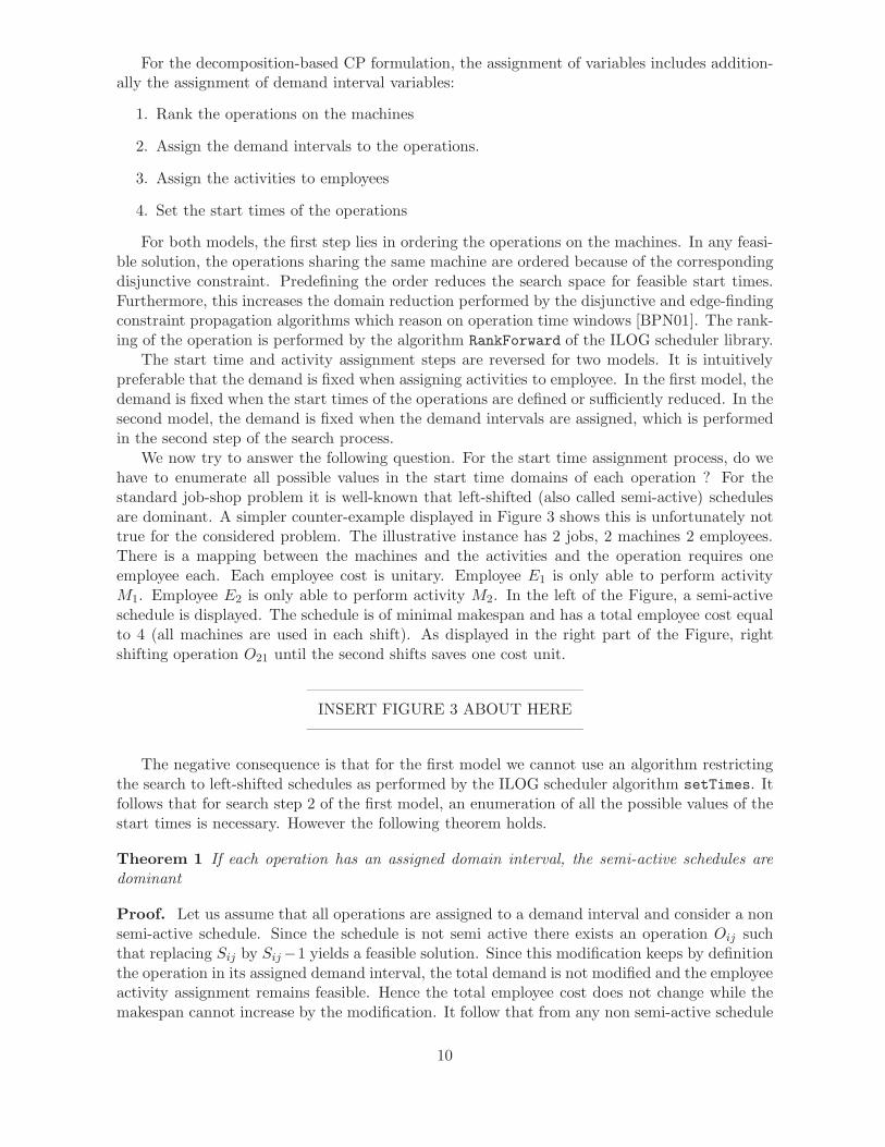
We now try to answer the following question. For the start time assignment process, do wehave to enumerate all possible values in the start time domains of each operation ? For thestandard job-shop problem it is well-known that left-shifted (also called semi-active) schedulesare dominant. A simpler counter-example displayed in Figure 3 shows this is unfortunately nottrue for the considered problem. The illustrative instance has 2 jobs, 2 machines 2 employees.There is a mapping between the machines and the activities and the operation requires oneemployee each. Each employee cost is unitary. Employee E1 is only able to perform activityM1. Employee E2 is only able to perform activity M2. In the left of the Figure, a semi-activeschedule is displayed. The schedule is of minimal makespan and has a total employee cost equalto 4 (all machines are used in each shift). As displayed in the right part of the Figure, rightshifting operation O21 until the second shifts saves one cost unit.

—————————————————–INSERT FIGURE 3 ABOUT HERE

—————————————————–

The negative consequence is that for the first model we cannot use an algorithm restrictingthe search to left-shifted schedules as performed by the ILOG scheduler algorithm setTimes. Itfollows that for search step 2 of the first model, an enumeration of all the possible values of thestart times is necessary. However the following theorem holds.

Theorem 1 If each operation has an assigned domain interval, the semi-active schedules aredominant

Proof. Let us assume that all operations are assigned to a demand interval and consider a nonsemi-active schedule. Since the schedule is not semi active there exists an operation Oij suchthat replacing Sij by Sij −1 yields a feasible solution. Since this modification keeps by definitionthe operation in its assigned demand interval, the total demand is not modified and the employeeactivity assignment remains feasible. Hence the total employee cost does not change while themakespan cannot increase by the modification. It follow that from any non semi-active schedule

10

we can obtain a semi-active schedules by applying a set of elementary modifications withoutdeteriorating the considered cost.

Consequently, for the last search step of the second model, only left-shifted schedules can beconsidered. The search algorithm setTimesForward of the ILOG scheduler library is used.

For the assignment of domain interval to operations, the enumeration is performed in thechronological order of the zones.

For the assignment of activities to employee we follow the following principle. We search forthe first period p for which the minimal demand for an activity a is not covered by the currentassignment of employees. This occurs when the number of employees for which variable Aes isfixed and set to a is lower than the smallest value in the domain of variable δas. In this case wesearch for the unassigned variable Aes that includes a in its domain that induces the minimalcost ceas. If no variable is found, a fail occurs. Otherwise, the branching is done by selectingvalue Aa for Aes in the left branch and by removing value a for domain s in the right branch.In the case the minimal demand is covered, the branching is done by assigning a rest activityA0 to the unassigned variable Aes with the smallest domain in the left branch and by removingthe rest activity for this variable in the right branch.

Several variants of the methods are compared on the following Section.

6 Instance generation and computational experiments

Since no previous work exists for the considered integration of the job shop problem and theemployee timetabling problem, we have developed an instance generator. The instance generatorhas been made as a java applet and is available on-line at the addresshttp://www.crt.umontreal.ca/∼adrien/instances.htm. The generator applet takes as input theproblem parameters as displayed in Figure 4. The number of extra employees parameters definesthe subset of “extras” employees able to perform all activities at a high cost. Such employees canbe added to allow the feasibility of the minimal makespan schedule and/or to obtain a feasibleinstance. Indeed in this paper we do not consider instances where the schedule feasibilityis limited by the employee availability. To solve such instances with our method, fictitiousextra employees with arbitrarily large costs have to be added. All costs concerning the regularemployees are generated between 1 and 5 to represent the preferences. All cost of extra employeeare equal to 9. Note these extra employees could in fact be outsourced personel or regular staffworking overtime

—————————————————–INSERT FIGURE 4 ABOUT HERE

—————————————————–

To test the proposed methods, we have generated several sets of instances. For each set theparameters are displayed in Table 3. We have generated 4 set of instances of increasing size wherea mapping between the resources and the activities exists and for which each operations requiresexactly one employee. The illustrative instance ejs1 belongs to this set. We have generated aset of instances where the mapping does not exists, defining 6 jobs, 4 machines, 5 activities and50 employees where each operation may require at most 2 activities simultaneously and at most2 employees for each activity. Except for series ejs, all instances are such that employees havethe required skills for 4 activities.

—————————————————–INSERT Table 3 ABOUT HERE

—————————————————–

11

As stated in Section 3, the lexicographic minimization problem is solved by first finding theminimum makespan through binary search. The makespan is then fixed to its minimal feasiblevalue and a second binary search is performed to minimize the total employee cost. A maximalCPU time limit of 1800 seconds is set to each backtrack search (i.e. to each iteration of thebinary searches). For constraint based scheduling we use ILOG Solver 6.1 and Scheduler 6.1.For LP resolution we use ILOG Cplex 9.1. All programs are coded in C++ under Linux on a64-bit AMD architecture.

Several variants of the method are tested. First, a pure CP resolution involving no LPrelaxation can be applied to the problem. The results of the resolution of the proposed directand decomposition-based CP formulations are displayed in Table 4 for a selection of 11 instancesof the 4 categories. For both the direct and the decomposition-based formulations, column M/Cgives the minimal makespan solution and its total employee cost. Columns CPU(F) gives theCPU times in seconds and the total number of fails needed to obtain the corresponding result.Note that for both formulation the minimal makespan solution is found for all instances in veryfast computational times. Therefore, we do not need to test any hybrid method for the makespanminimization on the instances we selected. Column C∗ gives the best upper and lower boundof the total cost obtained for the second phase. For both formulations and on all instances, themethod is unable to improve the initial employee cost. Indeed, the time limit of 1800 secondsis reached for each instance and each formulation (TL indication in the CPU(F) column). BothCP formulations appears inefficient to minimize the employee costs.

In the remaining, 12 variants of hybrid methods are compared to solve the employee costminimization at minimal makespan. The variants are obtained by the different possible com-binations of the values the following parameters. The first parameter is the used formulation(direct or decomposed). The second parameter is linked to reduced-cost based filtering, thatcan be switched on or off. The last parameter corresponds to the frequency of calls of the prop-agation algorithm of the LP global constraint (demandCover or demandIntervalCover). Thepropagation algorithms of the LP global constraint can be called at specified events, definingthe frequency of the LP resolution (and possibly the reduced cost-based filtering algorithms).The following propagation events (a), (b) and (c) are tested corresponding to increasing callfrequencies:

(a) when the lower bound of the per shift activity demand δas changes,

(b) when (a) holds or when the domain of an employee/activity assignment variable Aes ischanged,

(c) when (b) holds or when a demand interval variable Iij is fixed for an operation (only fordemandIntervalCover).

Intuitively, calling more frequently the LP resolution (and the reduced cost-based filtering al-gorithms) yields better pruning of the search tree at the possible expense of extra CPU times.Hence a good compromise has to be found.

The results of the direct and the decomposed formulations, with and without reduced costfiltering, are given in Table 5 for propagation rule (a) and in Table 6 for propagation rule (b).Last the results of the decomposition-based formulation only, with and without reduced costfiltering, are given in Table 7 for propagation rule (c). In each Table and for each parametercombination, column C∗ gives the optimal cost found by the method or the upper and lowerbound in the case the time limit is reached. Column CPU(F) gives the CPU time and thenumber of fails needed to obtain the optimal solution. TL indicates when the time limit isreached before getting the optimal solution. For each instance, the best result is displayed inbold (optimal found at minimal CPU time or best lower and upper bounds found).

12

The proposed methods are able to solve all instances but one (ejs10x10 3) to optimality.The theoretical superiority of the decomposition-based CP formulation and of its relaxation isverified in practice since the decomposed formulation obtains the best results on 9 instancesout of 11. For the direct formulation, the reduced cost-based filtering technique is very efficientsince the method can solve only 2 instances if this filtering method is switched off. With reducedcost-based filtering, the direct formulation solves all instances but one with propagation rule (a)only. The decomposition-based formulation solves also all instances but one with propagationrules (b) and (c), with and without reduced cost-based filtering. However the best results forthe decomposed formulation are obtained without reduced cost-based filtering for propagationrule (b). More precisely, for the decomposition formulation, using reduced cost-based filteringalways increases the CPU times, except for one instance (ejs8x8 1) with propagation rules (b)and (c) while it seems to reduce the CPU time for the solved instances with propagation rule (a).This could be interpreted by the fact that each reduction of an activity assignment of intervalvariable domain made by reduced cost-based filtering calls again the propagation of the globalLP constraints which calls again reduced-cost-based filtering, and so on. This process, carryingout too many calls of the propagation algorithm, could be limited by solving the LP relaxationand performing reduced-cost based filtering only once at each node of the search tree.

The experiments clearly show that the minimum cost is a lot smaller that the cost of theinitially found solution. However, this observation alone is not enough to argue in favor ofintegrated model: it lacks a third quantity: the minimal cost obtained if, in phase 2, not onlythe makespan was fixed, but all the scheduling variables. If this last quantity is close to theinitial cost solution, integration is valuable. If it is close to the min cost solution produced byphase 2 of the model, then integration is not valuable. This method is the one usually appliedin practice, that is to schedule first production and then the human resources

Table 8 shows the employee costs obtained by a sequential approach, after fixing for phase 2,the start time variables of the first minimal makespan solution. The solutions are obtained bythe decomposed formulation without reduced cost based filtering and propagation rule (b). Theinterest of integration appears clearly for 7 problems out of 11 for which the cost obtained by thenon-integrated approach varies from 4.8% to 36.5% above the cost obtained by the integratedapproach.

So far, we only considered the lexicographic order for the objective function. This order isnot always the best choice, because if they were an almost-minimal makespan schedule with afar smaller employee cost, it would certainly be preferable. Our last experiment, reported inTable 9, shows the solutions obtained by the integrated approach when the makespan cannotexceed 5% of the optimal makespan. We used the decomposed formulation without reduced costbased filtering and propagation rule (b). Although the problem becomes much more difficult tosolve for our approach (only 7 instances out of 11 are solved to optimality), the result show themethod can be helpful in a multiobjective framework using the epsilon-constraint method. Witha slight makespan increase (see column M) substantial cost gains (from 9.4% up to 29.5%) areobtained on 6 instances ou of 11. We note especially the large gains obtained for the instancesof the series ejs6x4x2x2 where there is no mapping between operations and activities, whichyields more flexibility for operator assignment. For the large instances however no solutionswith improving cost could be found.

We also point out that the epsilon-contraint method can be used to solve problems for whichthere is no possibility too hire extra employees. In this case, as stated above, extra employeescan be added with an arbitrarily large cost and the makespan can be progressively increaseduntil no extra employee is present in the solution.

13

7 Concluding remarks

The obtained results illustrate the potential cost savings brought by integrating employee timetablingand production scheduling. Indeed there is a significant difference for all instances between thecost of the initial makespan-minimal solution (column M/C of Table 4) and the final obtainedoptimal cost. There is also substantial employee cost improvements brought by the integratedmethod in comparison with a sequential approach. The method also showed its potential formultiobjective optimisation. Further research should focus on developing efficient heuristics forproblems of realistic size. We hope the exact method we developed in this study will be usefulto evaluate the quality of the heuristics.

The computational experiments we have carried out on a set of randomly generated instancesconfirms the theoretical interest of the proposed decomposition-based CP formulation of theintegrated employee timetabling and production scheduling problem and of its associated LPrelaxation. The key point of the decomposition lies in the possibility of restricting to semi-active schedules as soon as intervals have been assigned to operations. The main interest of theproposed LP relaxation is to incorporate aggregated scheduling decisions in the LP model withthe help of energetic reasoning concepts.

Reduced cost-based filtering techniques confirm their interest for integrated planning andscheduling problems. However, depending on the used formulation and LP relaxation, thefrequency of calls of the propagation algorithms have to be tuned carefully. In all cases, thehybrid method were able to obtain optimal solutions for the employee-cost minimization problemat minimal makespan while pure CP-based method could not improve the initial cost. The resultswe obtained illustrate that (hybrid) methods have to be designed taking account of the structureand properties of the particular problem with the help of scheduling theory.

References

[AB97] H. Alfares and J. Bailey. Integrated project task and manpower scheduling. IIETransactions, 29(9):711–717, 1997.

[BAL95] J. Bailey, H. Alfares, and W. Lin. Optimization and heuristic models to integrateproject task and manpower scheduling. Computers and Industrial Engineerings,29:473–476, 1995.

[BC94] N. Beldiceanu and E. Contejean. Introducing global constraints in chip. Journal ofMathematical and Computer Modelling, 20(12):97–123, 1994.

[BDP96] J. Blazewicz, W. Domschke, and E. Pesch. The job shop scheduling problem: Con-ventional and new solution techniques. European Journal of Operational Research,93:1–33, 1996.

[BGAB83] L. Bodin, B. Golden, A. Assad, and M. Ball. Routing and scheduling of vehicles andcrews the state of the art. Computers and Operations Research, 10(2):63–211, 1983.

[BGHS05] P. Baptiste, V. Giard, A. Haıt, and F. Soumis, editors. Gestion de production etressources humaines. Presses Internationales Polytechnique, 2005.

[BP96] Ph. Baptiste and C. Le Pape. Disjunctive constraints for manufacturing scheduling:Principles and extensions. International Journal of Computer Integrated Manufac-turing, 9(4):306–310, 1996.

14

[BPN01] Ph Baptiste, C. Le Pape, and W. Nuijten. Constraint-Based Scheduling. Kluwer,2001.

[Che04] Z. Chen. Simulataneous job scheduling and resource allocation on parallel machines.Annals of Operations Research, 129:135–153, 2004.

[CSSD01] J.-F. Cordeau, G. Stojkovic, F. Soumis, and J. Desrosiers. Benders decomposition forsimultaneous aircraft routing and crew scheduling. Transportation science, 35:375–388, 2001.

[DB06] L.-E. Drezet and J.-C. Billaut. Predictive and proactive approaches for RCPSP withlabour constraints. In 12th IFAC Symposium on Information Control Problems inManufacturing (INCOM06), Saint-Etienne, 2006.

[DDI+98] G. Desaulniers, J. Desrosiers, I. Ioachim, M.M. Solomon, F. Soumis, and D. Vil-leneuve. A unified framework for deterministic time constrained vehicle routing andcrew scheduling problems. In T. Crainic and G. Laporte, editors, Fleet managementand logistics, pages 57–93. Kluwer, 1998.

[DHM96] R. L. Daniels, B. J. Hoopes, and J. B. Mazolla. Scheduling parallel manufacturingcells with resource flexibility. Management science, 42:1260–1276, 1996.

[DM94] R. L. Daniels and J. B. Mazolla. Flow shop scheduling with resource flexibility.Operations Research, 42(3):504–522, 1994.

[DMS04] R. L. Daniels, J. B. Mazolla, and D. Shi. Flow shop scheduling with partial resourceflexibility. Management Science, 50(5):658–669, 2004.

[DPR05] S. Demassey, G. Pesant, and L.-M. Rousseau. Constraint programming based columngeneration for employee timetabling. In 7th International Conference on Integrationof AI and OR techniques in Constraint Programming for Combinatorial OptimizationProblems (CPAIOR’05), Prague, 2005.

[EJKS04] A.T. Ernst, H. Jiang, M. Krishnamoorthy, and D. Sier. Staff scheduling and roster-ing: A review of applications, methods and models. European Journal of OperationalResearch, 153:3–27, 2004.

[ELT89] J. Erschler, P. Lopez, and C. Thuriot. Scheduling under time and resource con-straints. In Proc. of Workshop on Manufacturing Scheduling, 11th IJCAI, Detroit,USA, 1989.

[FHW03] R. Freling, D. Huisman, and A. Wagelmanss. Models and algorithms for integrationof vehicle and crew scheduling. Journal of Scheduling, 6(1):63–85, 2003.

[FLM99] F. Focacci, A. Lodi, and M. Milano. Cost-based domain filtering. In Fifth Interna-tional Conference on the Principles and Practice of Constraint Programming CP’99,volume 1713 of Lecture Notes in Computer Science, pages 189–203. Springer-Verlag,1999.

[FLN00] F. Focacci, P. Laborie, and W. Nuijten. Solving scheduling problems with setuptimes and alternative resources. In AIPS, pages 92–111, 2000.

[HBBF05] A. Haıt, P. Baptiste, N. Brauner, and G. Finke. Approches integrees a court terme,2005. chapter 6 in [BGHS05].

15

i mij pij

1 3 2 0 1 3 7 2 92 3 0 1 2 8 10 3 13 2 1 3 0 3 4 8 64 1 3 0 2 10 3 3 95 2 0 3 1 10 8 4 76 2 1 0 3 2 3 10 4

Table 1: Job data

[HCM04] F. Huq, K. Cutright, and C. Martin. Employee scheduling and makespan mini-mization in a flow shop with multi-processor work stations: a case study. Omega,32:121–129, 2004.

[HF99] K. Haase and C. Friberg. An exact algorithm for the vehicle and crew schedulingproblem. In N. Wilson, editor, Computer-Aided Transit Scheduling, volume 471 ofLecture Notes in Economics and Mathematical Systems, pages 63–80. Springer, 1999.

[Hoo05] J. N. Hooker. A hybrid method for planning and scheduling. Constraints, 10:385–401,2005.

[KJN02] D. Klabjan, E.L. Johnson, and G.L. Nemhauser. Airline crew scheduling with timewindows and plane count constraints. Transportation science, 36:337–348, 2002.

[MCS05] A. Mercier, J.-F. Cordeau, and F. Soumis. A computational study of benders decom-position for the integrated aircraft routing and crew scheduling problem. Computersand Operations Research, 32:1451–1476, 2005.

[Pes04] G. Pesant. A regular language membership constraint for finite sequences of vari-ables. In Tenth International Conference on Principles and Practice of ConstraintProgramming -CP’04, volume 3258 of Lecture Notes in Computer Science, pages482–495. Springer-Verlag, 2004.

[Reg96] J.-C. Regin. Generalized arc consistency for global cardinality constraint. InAAAI/IAAI, pages 209–215. AAAI Press/The MIT Press, 1996.

[TO02] E. S. Thorsteinsson and G. Ottoson. Linear relaxations and reduced-cost basedpropagation of continuous variable subscripts. Annals of operations research, 115:15–29, 2002.

[vPRS06] W.-J van Hoeve, G. Pesant, L.-M. Rousseau, and A. Sabharwal. Revisiting thesequence constraint. In CP-06. Proceedings of the 12th International Conference onPrinciples and Practice of Constraint Programming, Nantes, 2006. to appear.

16

e a ceas

1 2 5 4 2 1 4 1 5 54 3 4 4 4 2 4 4 4

2 1 4 2 2 1 2 4 3 13 5 4 4 4 1 1 2 2

3 1 2 2 1 1 5 3 2 14 4 5 1 2 4 3 5 1

4 2 5 2 4 1 5 3 1 43 1 2 5 4 3 3 4 3

5 2 4 4 4 2 4 5 2 53 5 5 2 1 3 3 2 2

6 1 2 4 4 5 4 2 5 54 5 2 1 5 4 3 1 4

7 3 5 2 1 3 1 4 3 14 2 3 5 3 5 4 5 3

8 1 5 5 1 1 5 4 3 22 1 4 1 5 3 1 5 1

9 1 3 3 3 3 3 2 2 12 1 5 5 2 5 3 3 5

10 3 3 5 1 3 4 4 4 14 5 5 1 5 4 1 3 1

11 2 5 4 2 4 1 3 2 13 5 1 5 2 5 2 3 1

12 1 3 2 3 4 2 1 2 44 4 5 5 1 3 1 2 5

13 1 5 5 4 2 3 5 4 54 2 3 2 3 1 3 4 2

14 2 5 3 3 5 1 2 3 53 5 4 2 5 2 5 5 3

15 1 4 1 2 2 2 1 5 44 1 2 5 3 5 4 1 4

Table 2: Employee data

17

O41 O54 O23

O51 O12 O44

O21 O42 O64 O33O53

O61

O13

O11

O31

O62 O32

O63 O52 O34O43 O22

O14

M1

M2

M3

M4

E1

E2

E3

E4

E5

E6

E7

E8

E9

E11

E12

E13

E14

E15

M2, 2 M2, 1

M1, 2

M2, 1

M3, 2

M4, 2

M1, 2

M3, 1

M1, 1

M3, 1

M2, 1

M4, 1

M3, 1 M3, 2

M4, 1

M4, 1

M2, 3 M2, 1

M1, 1

M1, 1 M1, 1

0 8 16 24 32 40 48

E10

O24

Figure 1: Optimal solution of the EJS1 instance

Inst name n m µ extra α mapping σ π max act max empl max skillper oper per act per empl

ejs 6 4 25 10 4 yes 8 8 1 1 2ejs8x8 8 8 40 20 8 yes 8 8 1 1 4ejs10x10 10 10 50 20 10 yes 10 10 1 1 4ejs6x4x2x2 6 4 50 20 5 no 9 10 2 2 4

Table 3: Parameters of the generated instances

18

6

I0 I1 I2 I3 I4

ESij LSij

0 1 2 3 54

s

δija

0

1I1

0 1 2 3 54

s

δija

0

1I2

0 1 2 3 54

s

δija

0

1I3

0 1 2 3 54

s

δija

0

1I4

6

6

6

6

0 1 2 3 54

s

δija

0

1I0

Oij

Figure 2: Decomposition of a start time domain in demand intervals

E2

O11

M2, 1

M1

M2

E1 M1, 1 M1, 1

M2, 1

M1

M2

E1

E2

Makespan=8 Employee cost=4 Makespan=8 Employee cost=3

O12O21

M1, 1

M2, 1

M1, 1

O12

O22O22

O21

O11

Figure 3: Non dominance of semi-active schedules

19

Figure 4: Instance generator applet

Direct DecompositionInst M/C CPU(F) C∗ CPU(F) M/C CPU(F) C∗ CPU(F)ejs4 40/27 0.1(3) 27(13) TL 40/27 0.1/3 27(14) TLejs9 49/44 0.2(4) 44(0) TL 49/44 0.2(4) 44(0) TLejs10 48/38 0.2(3) 38(0) TL 48/38 0.2(3) 38(0) TLejs8x8 1 44/135 0.7(65) 135(0) TL 44/135 0.7(65) 135(0) TLejs8x8 2 51/161 0.7 (6) 161(0) TL 51/161 0.7(6) 161(0) TLejs8x8 3 44/123 0.7(24) 123(0) TL 44/123 0.7(24) 123(0) TLejs10x10 1 80/182 1.8 (145) 182(0) TL 80/182 1.6(145) 182(0) TLejs10x10 3 84/150 7.4(2164) 150(0) TL 84/150 12(5268) 150(0) TLejs6x4x2x2 1 46/223 0.64 (18) 223(0) TL 46/223 0.64(18) 223(0) TLejs6x4x2x2 2 54/182 0.6(9) 184(0) TL 54/182 0.6(9) 184(0) TLejs6x4x2x2 3 42/240 0.7(16) 240(0) TL 42/240 0.7(16) 240(0) TL

Table 4: Results of pure CP methods

20

Direct + demandCover Decomposition + demandIntervalCover

no RC with RC no RC with RCInst C∗ CPU(F) C∗ CPU(F) C∗ CPU(F) C∗ CPU(F)ejs4 23 2269(441635) 23 1.0(4) 25(23) TL 23 2.0 (2587)ejs9 44(0) TL 24 135(6120) 24 194 (52328) 24 50.4 (7770)ejs10 38(13) TL 23 5.1(159) 38(16) TL 23 27.1(22838)ejs8x8 1 135(69) TL 78 133(1225) 135(77) TL 135 (77) TLejs8x8 2 161(86) TL 96 155(869) 161(92) TL 161 (92) TLejs8x8 3 123(67) TL 83 52(203) 123(72) TL 123(72) TLejs10x10 1 182(92) TL 124 2690(14176) 182(102) TL 182(102) TLejs10x10 3 150(76) TL 150(15) TL 150(15) TL 150 (15) TLejs6x4x2x2 1 223(16) TL 132 50(902) 223(40) TL 223(40) TLejs6x4x2x2 2 184(0) TL 74 225(2431) 184(22) TL 184(22) TLejs6x4x2x2 3 240(122) TL 148 29(217) 240(133) TL 240(133) TL

Table 5: Results of CP with LP propagation on bound change of δas

Direct + demandCover Decomposition + demandIntervalCover

no RC with RC no RC with RCejs4 23 0.7(8) 23 0.7(4) 23 0.8(8) 23 0.8(4)ejs9 44(0) TL 44(0) TL 24 61(11128) 24 121(7465)ejs10 38(13) TL 38(13) TL 23 2.6(219) 23 3.8 (159)ejs8x8 1 135(69) TL 135(69) TL 78 90(3310) 78 81.2(1437)ejs8x8 2 123(86) TL 104(86) TL 96 103(1679) 96 107(848)ejs8x8 3 83 40(1602) 83 64(736) 83 29(227) 83 34(204)ejs10x10 1 182(92) TL 182(92) TL 124 926(24125) 124 1518(19224)ejs10x10 3 150(76) TL 150(0) TL 150(15) TL 150(15) TLejs6x4x2x2 1 223(16) TL 223(16) TL 132 38(1304) 132 40.3(977)ejs6x4x2x2 2 184(0) TL 184(0) TL 74 157(2781) 74 194(2398)ejs6x4x2x2 3 181(122) TL 181(122) TL 148 24(332) 148 24(224)

Table 6: Results of CP with LP propagation on bound change of δas and on assignment of Aes

Decomposition + demandIntervalCover

no RC with RCInst C∗ CPU(F) C∗ CPU(F)ejs4 23 1.0(8) 23 1.0(4)ejs9 24 79(9643) 24 141(6120)ejs10 23 3.55(217) 23 5.08(159)ejs8x8 1 78 156(3207) 78 134(1225)ejs8x8 2 96 156(1679) 96 172(869)ejs8x8 3 83 46(227) 83 53(203)ejs10x10 1 124 1893(21314) 124 2832(14176)ejs10x10 3 150(15) 1811(9202) 150(15) 1812(8203)ejs6x4x2x2 1 132 50(1304) 132 50(902)ejs6x4x2x2 2 74 173(2777) 74 225(2431)ejs6x4x2x2 3 148 29(332) 148 29(217)

Table 7: Results of CP with propagation of LP constraint on δas bound change, Aes and Iij

assignment

21

Decomposition + demandIntervalCover

no RCInst C∗ CPU(F) lossejs4 23 0.95(8) 0%ejs9 24 5.13(755) 0%ejs10 28 2.3(127) 21%ejs8x8 1 91 11.6(196) 16.6%ejs8x8 2 110 159(2968) 14.6%ejs8x8 3 98 11.07(69) 18%ejs10x10 1 130 157(1902) 4.8%ejs10x10 3 150(83) 1927(29840) 0%ejs6x4x2x2 1 132 27.8(654) 0%ejs6x4x2x2 2 101 7.3(71) 36.5%ejs6x4x2x2 3 170 8.28(113) 14.8%

Table 8: Results of the sequential approach

Decomposition + demandIntervalCover

no RCInst M C∗ CPU(F) gainejs4 40 23 0.95(8) 0%ejs9 49 24 67(11128) 0%ejs10 48 23 15(1589) 0%ejs8x8 1 46 68(61) 3207(114975) 12.8%ejs8x8 2 52 87(79) 2675(122407) 9.4%ejs8x8 3 46 72 5027(141410) 13.3%ejs10x10 1 80 182(19) 1801(30777) -46%ejs10x10 3 84 150(14) 1811(47248) 0%ejs6x4x2x2 1 48 93 49(1010) 29.5%ejs6x4x2x2 2 56 58 718(16134) 21.6%ejs6x4x2x2 3 43 118 745(19228) 20.2%

Table 9: Results of the integrated approach for a makespan within 5% of the minimal makespan

22