solving di erential algebraic equations by taylor series … (that is, enclosures of the solutions)...

European Society of Computational Methodsin Sciences and Engineering (ESCMSE)

Journal of Numerical Analysis,Industrial and Applied Mathematics

(JNAIAM)vol. 3, no. 1-2, 2008, pp. 61-80

ISSN 1790–8140

Solving Differential Algebraic Equations byTaylor Series (III): the Daets Code1

Nedialko S. Nedialkov 2

Department of Computing and Software, McMaster University,Hamilton, Ontario, L8S 4L7, Canada

John D. Pryce 3

Department of Information Systems, Cranfield University,RMCS Shrivenham, Swindon SN6 8LA, UK

Received 30 October, 2007; accepted in revised form 26 January, 2008

Abstract: The authors have developed a Taylor series method for solving numericallyan initial-value problem differential algebraic equation (DAE) that can be of high index,high order, nonlinear, and fully implicit, see BIT 45:561–592, 2005 and BIT 41:364-394,2001. Numerical results have shown this method to be efficient and very accurate, andparticularly suitable for problems that are of too high an index for present DAE solvers.This paper outlines this theory and describes the design, implementation, usage and per-formance of Daets, a DAE solver based on this theory and written in C++.

c© 2008 European Society of Computational Methods in Sciences and Engineering

Keywords: Differential algebraic equations (DAEs), structural analysis, Taylor series, au-tomatic differentiation

Mathematics Subject Classification: 34A09, 65L80, 65L05, 41A58

1 Introduction

1.1 What Daets does and the tools it uses

This paper describes the structure and use of a code Daets (Differential Algebraic Equations byTaylor Series) that solves initial value problems for differential algebraic equation systems (DAEs)for state variables xj(t), j = 1, . . . , n, of the general form

fi( t, the xj and derivatives of them ) = 0, i = 1, . . . , n, (1)

by expanding the solution in a Taylor series (TS) at each integration step. The fi can be arbitraryexpressions built from the xj and t using +,−,×,÷, other analytic standard functions, and the

1Published electronically March 31, 20082Corresponding author. E-mail: [email protected]: [email protected]

62 N. S. Nedialkov and J. D. Pryce

differentiation operator dp/dtp. They can be nonlinear and fully implicit in the variables andderivatives. An equation such as

((tx′1)′)2

1 + (x′2)2+ t2 cosx2 = 0 (2)

can be encoded directly into Daets. Derivatives need not actually be present, so Daets can solvecontinuation problems f(t,x) = 0, taking t as the continuation parameter. It has handled difficultproblems of this kind, as reported in Subsection 5.3.

A common measure of the numerical difficulty of a DAE is its differentiation index νd, thenumber of times the fi must be differentiated (w.r.t. t) to obtain equations that can be solved toform an ODE system for the xj . Index ≥ 3 is normally considered hard. Daets is not inherentlyaffected by high index, as explained later. We report results on up to index-47 DAEs.

One of the hardest parts of DAE solution can be finding an initial consistent point. This canbe seen as a minimization problem, and Daets gives this task to a proven optimization packageIpopt [28], which has proved robust and effective.

Stiff behaviour can be present for DAEs, as for ODEs. Daets, like other codes based on Taylorseries, handles moderate stiffness well but is unsuitable for highly stiff problems.

Daets is not a validating code that finds guaranteed enclosures of the exact solution. Theauthors know in principle how to implement such a code, but it is a large project.

Daets is written in C++. Apart from Ipopt, it uses Stauning’s automatic differentiation (AD)package Fadbad++ [27] and the C version of Volgenant’s LAP [11] code for Linear AssignmentProblems.

The rest of this introduction takes a software developer’s viewpoint. Subsection 1.2 reviewstheoretical approaches to DAEs based on derivatives of equations, as is that of Daets; and de-scribes the origins of the software architecture of Daets. Subsection 1.3 gives a broad overview ofthe numerical method, and discusses the impact it has on the architecture and the user interface.

Following this, Section 2 outlines the structural analysis (SA) theory on which the numericalmethod is based. Section 3 describes the main components of the algorithm. Section 4 discussesthe user-visible classes, and other user interface matters. Section 5 reports and discusses the perfor-mance of the code on various problems. Section 6 shows a simple complete program using Daets.Section 7 summarises our experience with Daets and describes some outstanding problems.

1.2 Background

Many problems of importance in science and industry are modelled as DAEs. Examples from ap-plications are in the Test Set for Initial Value Solvers [14], which contains problems from electroniccircuits, mechanical systems and chemical processing. One reason why higher index DAEs are ofinterest because adding detail to a model, such as accounting for internal behaviour of actuatingmotors in a robot arm, often raises the index.

For a traditional solver, the problem is typically written as a first-order ODE x′ = f(t,x) orfirst-order DAE M(t,x)x′ = f(t,x), where M is a singular matrix. The code only sees a “blackbox” routine that computes the value of f or M or (for stiff problems) Jacobian information atgiven inputs (t,x). It has long been known in various theoretical frameworks that a DAE can beseen as an ODE on a manifold and can be accurately solved as such, provided one “knows” how tomanipulate derivatives of the defining functions. This underlies the jet space approach [25] basedon differential geometry, Campbell’s derivative array theory [4] and more practical approaches ofindex reduction [1, 13]. Daets is based on Pryce’s structural analysis [24], which has this samebasic approach and is itself an extension of the method of Pantelides [19].

As regards using Taylor series to solve DAEs, we believe this was first done by Chang [5], in anad hoc way. The software architecture of Daets is derived from that of Nedialkov’s Vnode code

c© 2008 European Society of Computational Methods in Sciences and Engineering (ESCMSE)

Solving DAEs by Taylor Series (III): DAETS 63

[15] mainly written during his PhD project at the University of Toronto. Vnode finds validatedsolutions (that is, enclosures of the solutions) of ordinary differential equation (ODE) initial valueproblems, using interval arithmetic. More important than the interval aspect is that Vnode isan object-oriented implementation of a general design for ODE solvers due to Hull and Enright[10]. This design separates parts of the algorithm into modules, such as the stepping formula, errorestimation, step size choice, output to the user, etc., in a way that makes it easy to change thealgorithm for one part with minimal impact on the others.

Daets and Vnode have in common parts of the implementation as well as of the design:for instance they both use Fadbad++ to do AD, and Vnode has an optional stepping modulethat uses TS. However, Daets handles the implicit system (1) while Vnode handles an explicitODE system x′ = f(t,x), which makes a large difference to the details of how the two codes useFadbad++ and how they generate Taylor coefficients (TCs). Some significant parts of the Daetsalgorithm have no counterpart in the Hull–Enright design.

1.3 The method and how it affects the design

We describe in broad terms the numerical method based on Pryce’s structural analysis (SA) [23, 24],and discuss how its features affect the design of the code, especially the user interface. In thissubsection, “software” means our (or another) DAE solver, as opposed to the infrastructure toolsbelow it or an application on top of it.

The numerical method. Starting with code for the functions fi in (1), an SA-based method usesautomatic differentiation (AD) to evaluate suitable derivatives dr/dtr of the fi. By equating theseto zero at a given t = t, it solves implicitly for derivatives, or equivalently TCs, of the solutioncomponents xj(t) at t.

The AD can be handled in many ways, depending on language features and on the tools oneconsiders efficient and convenient. We use Ole Stauning’s popular AD tool, Fadbad++, whichuses C++ templates and operator overloading to compute derivatives. There is evidence thatother tools may give somewhat faster code, e.g. Adol-C [7], but we have found Fadbad++ isconvenient for the software writer, allows a straightforward user interface, and has to date causedno problems with installing the software.

As illustrated in (2), differentiation d/dt can be used anywhere in the expressions defining theDAE. To enable this, Stauning modified Fadbad++ to make d/dt a “first-class” operator (nameddiff), like the arithmetic operations and standard functions. Also, to make over/underflow lesslikely in computing coefficients ar of a Taylor expansion a(t∗ + h) =

∑r arh

r, Daets computesthe terms arh

r directly. This is neatly done by an implicit change of independent variable fromt to s, where t = t∗ + sh. This required creating our version of the d/dt operator (named Diff)inside Daets, so Fadbad++ is not changed.

Various numerical methods can be based on SA. “Solving implicitly” can in effect reduce theDAE to an ODE system — numerically implementing the definition of the differentiation index— and a standard method such as Runge–Kutta or BDF can be applied to the result. Methodsof this kind are starting to be studied. We have chosen the approach in Pryce’s original papers,using the AD to evaluate the TS to some order. The resulting method is generally not as efficientas standard DAE solvers on problems they can solve, but becomes increasingly efficient at highaccuracies and is relatively simple to code.

In the SA one computes the n×n signature matrix, and 2n integers, the offsets of the variablesand of the equations. These prescribe the overall process for computing TCs, as well as how toform the System Jacobian J (5) that is central to the theory and the numerical method.

The TCs are used with an appropriate stepsize to find a truncated TS approximation of thesolution, which is then projected to satisfy the constraints of the DAE. The process is repeated on



each integration step in a standard time-stepping manner. Error estimation and step size selectionare like that in Taylor codes for ODEs, but the offsets complicate the details.

If J is nonsingular at a consistent point, see Subsection 2.3, the SA has succeeded, and theDAE is solvable in a neighborhood of this point. Although SA applies to a wide range of DAEs,there are problems on which it fails: when J is singular at a point at which the DAE is solvable.Typically this happens when the equations (1) are “not sparse enough” to reveal the underlyingstructure of the system. Examples are discussed in [16, 23, 24].

An SA-based method derives a structural index νs, which is the same as the index found bythe method of Pantelides [19] for DAEs to which that method applies. It is shown by Reißig,Martinson and Barton [26] that νs can be arbitrarily greater than νd; but in [24, Subsection 5.3],that provided the SA succeeds — that is, J is nonsingular — νs can never be less than νd, andin [16] that overestimating νs causes, at worst, mild inefficiency in the solution process. Moreoverthe method is robust in the sense that it can always detect (up to roundoff) when J is singular,and therefore indicate that the SA fails: see [16, Algorithm 6.1].

Effect on the user interface. C++ code for the functions fi in (1) looks much as for a standardODE solver for y′ = f(t,y). However, the active variables must be declared of a templated type,instantiated at compile time with several different actual types. One type is used for the numericalAD, another to compute the signature matrix, and so on. This imposes some restrictions on theallowed expressions. Also, the differentiation operator Diff(·,q) denoting dq/dtq can be appliedto any active item. The latter are the inputs x[j] denoting xj , the outputs f[i] denoting fi, andany code variables or expressions on the computational path between these.

When the SA method succeeds, it gives the user much useful information about the structureof the DAE. We provide a way for the calling program to print the signature matrix, offsets andrelated data after the SA has been done. In fact the user needs to know SA data to use an SA-basedmethod effectively, because the offsets determine the shape of the set of initial values to be givento the solver (fixed values, or free, guessed, values). For traditional ODE/DAE solvers, the initialvalues are flat vectors: here they form an irregular array, see page 71.

Coding the calling program for an unfamiliar DAE tends to be a two-stage process. First, givethe function code to Daets and make it print a description of the structure. Setting initial valuescan then be coded correctly, although it may need thought about their physical meaning to get asensible choice of fixed and free values.

The fact that analysis precedes numerical solution affects the user interface. First, it is whythe interface makes two (main) classes available. One, DAEsolution, holds the irregular arrayof xj-and-derivatives at a given t, plus related data. The other, DAEsolver, knows among otherthings the result of the structural analysis. Its integrate method can be applied to differentDAEsolution objects. Thus one can compute many solution paths without re-doing the SA.

Second, each stage has its own kind of error. The SA can find there is no finite transversal(Subsection 2.1), indicating an ill-posed problem. Or the SA can appear to succeed, but theresulting Jacobian matrix J is always singular, showing the SA doesn’t reveal the true structureof the DAE. Or the code may find a nonsingular J but be unable to find a consistent point. Or itmay find a consistent point and start along the solution path, but grind to a halt for some reason.

The two-way information flow in preparing the problem for solution gives Daets some featuresof a Problem Solving Environment. We do not offer an interactive GUI yet, but this would beuseful. There is a contrasting requirement, however. The software may be needed as an “engine”,to solve a DAE of known structure as part of a larger application. For such use, it must suppressprinting and return any error diagnostics by a flag (or similar) that is handled by the callingprogram. Daets can be used in such a silent mode as well as in a verbose one.



2 Theory

2.1 Pryce’s structural analysis of DAEs

We present as much of Pryce’s structural analysis [24] as is needed for this paper.A transversal T of an n× n matrix (σij) is a set of n positions in the matrix with one entry in

each row and each column — a set {(1, j1), (2, j2), . . . , (n, jn)} where (j1, . . . , jn) are a permutationof (1, . . . , n). The value of T is ValT =

∑(i,j)∈T σij .

Given a DAE in the form of (1), we perform the following steps.

1. Form the n× n signature matrix Σ = (σij), where

σij =

order of the derivative to which the jth variable xj occurs inthe ith equation fi; or

−∞ if xj does not occur in fi.

2. Find a highest value transversal (HVT), which is a transversal T that makes ValT as largeas possible. This value is also, by definition, the value of the signature matrix, written Val Σ.

The value of any transversal, and of Σ, is either an integer or −∞. The DAE is structurallyregular if Val Σ is finite: that is, if at least one transversal exists, all of whose σij are finite.Otherwise it is structurally ill-posed — probably the problem is wrongly posed in some way.

3. Find n-dimensional integer vectors c and d, with all ci ≥ 0, that satisfy

dj − ci ≥ σij for all i, j = 1, . . . , n and (3)

dj − ci = σij for all (i, j) ∈ T . (4)

By [24, Lemma 3.3], if a transversal T and vectors c,d are found such that (3) and (4) hold,then necessarily T is a HVT. Summing (4) over T gives an alternative formula for Val Σ:

n∑

j=1

dj −n∑

i=1

ci = ValT = Val Σ.

It follows that for any c and d, if (3, 4) hold for some HVT, then (4) holds for any HVT.

The vectors c and d are the offsets. They are never unique. It is a little more efficient, butnot necessary, to choose the canonical offsets, which are the smallest in the sense of a ≤ b ifai ≤ bi for each i.

4. Form the n× n System Jacobian matrix

J =∂(f

(c1)1 , . . . , f

(cn)n

)

∂(x

(d1)1 , . . . , x

(dn)n

) . (5)

By results in [24], equation (5) has the equivalent formulation:

Jij =∂fi

∂x(dj−ci)j

=

∂fi

∂x(σij)j

if dj − ci = σij , and

0 otherwise.

(6)



5. Seek values for the xj and for appropriate derivatives, consistent with the DAE in the senseof Subsection 2.3, at which J is nonsingular. If such values exist, they define a point throughwhich there is locally a unique solution of the DAE. In this case we say the method “succeeds”.

Step (2) is a Linear Assignment Problem (LAP), a form of a linear programming problem forwhich good software exists [11]. Step (3) defines its dual. The two formulae for Val Σ instance thefact that primal and dual have the same optimal value.

When the method succeeds:

• Val Σ equals the number of degrees of freedom (DOF) of the DAE, that is the number ofindependent initial conditions required.

• An upper bound for the differentiation index νd is given by the Taylor index

νT = maxici +

{1 if some dj is zero,0 otherwise.

(7)

In many cases, νT = νd.

2.2 An example

In this paper, we give examples based on the simple pendulum, a DAE of differentiation-index 3.Although it is small, solving it with our method displays almost all the algorithmic features. It is:

0 = f = x′′ + xλ

0 = g = y′′ + yλ−G0 = h = x2 + y2 − L2.

(8)

Here gravity G and length L of pendulum are constants, and the dependent variables are thecoordinates x(t), y(t) and the Lagrange multiplier λ(t).

A signature matrix Σ may be shown by a “tableau”, which annotates it with the offsets ci, djand the function and variable names, and marks the positions of a HVT. For (8), there are twoHVTs, marked • and ◦ in the tableau below. The canonical offsets are c = (0, 0, 2) and d = (2, 2, 0):

x y λ ci[ ]f 2• −∞ 0◦ 0

g −∞ 2◦ 0• 0

h 0◦ 0• −∞ 2

dj 2 2 0

(9)

For this system, (6) gives the system Jacobian

J =

∂f/∂x′′ 0 ∂f/∂λ

0 ∂g/∂y′′ ∂g/∂λ

∂h/∂x ∂h/∂y 0

=

1 0 x0 1 y

2x 2y 0

.

From (7) the Taylor index is 3, agreeing with the differentiation index.

2.3 Consistent points and quasi-linearity

The offsets specify what data is needed to define a consistent point, and what consistent means.Namely, the data comprise a point

X =(x1, x

′1, . . . , x

(d1−1)1 ; x2, x

′2, . . . , x

(d2−1)2 ; . . . ; xn, x

′n, . . . , x

(dn−1)n

). (10)



It is consistent iff it satisfies the set of equations

F =(f1, f

′1, . . . , f

(c1−1)1 ; f2, f

′2, . . . , f

(c2−1)2 ; . . . ; fn, f

′n, . . . , f

(cn−1)n

)= 0. (11)

An xj whose dj is zero (it must have σij = 0 for all i and thus is a “purely algebraic variable”)does not appear in the vector X. Similarly, an fi with ci = 0 does not appear in F.

f ′i means dfi/dt treating the variables and their derivatives as (unknown) functions of t, forinstance if f1 = x′′1 − x1x3 then f ′1 = x′′′1 − x′1x3 − x1x

′3; similarly for higher derivatives.

A convenient notation for such “irregular vectors” is as follows. If J is a set of indices (j, r)

where 1 ≤ j ≤ n and r ≥ 0, let xJ denote the set of derivatives x(r)j for (j, r) ∈ J , regarded as a

vector. Use the notation J≤k [resp. J<k] to mean the set of (j, r) satisfying 0 ≤ r ≤ k + dj [resp.

0 ≤ r < k + dj ]. For a similar set of indices I, let fI denote the derivatives f(r)i for (i, r) ∈ I, and

let I≤k [resp. I<k] mean the set of (i, r) satisfying 0 ≤ r ≤ k + ci [resp. 0 ≤ r < k + ci].Then (10, 11) can be written

fI<0(xJ<0

) = 0. (12)

There is an amendment to the above definition of X and F. Daets checks whether the nextderivatives after those in (10), namely x

(dj)j , j = 1, . . . , n, occur in a jointly linear way in the fi.

If they do, we call the DAE quasi-linear, by analogy with a similar notion in PDE theory.

If the DAE is not quasi-linear, these next derivatives x(dj)j are included in X and corresponding

derivatives of the fi, namely f(ci)i = 0, i = 1, . . . , n, are included in the equations (11) that define

a consistent point. That is, (12) changes to

fI≤0

(xJ≤0

)= 0. (13)

Define α = −1 if the DAE is quasi-linear, and α = 0 otherwise. Then write both (12) and (13) as

fI≤α(xJ≤α

)= 0. (14)

For example, in the Pendulum system (8), the relevant derivatives x(dj)j are x′′, y′′ and λ. Their

occurrence is jointly linear, so (8) is quasi-linear. It would still be so were, say, f changed tox′′x+ xλ or to x′′y′ + xλ, but not if it were changed to x′′y′′ + xλ, or to x′′λ+ xλ.

In the original quasi-linear case, the equations (12) for a consistent point are

Solve h, h′ = 0 for x, x′, y, y′.

When not quasi-linear, they become

Solve f, g, h, h′, h′′ = 0 for x, x′, x′′, y, y′, y′′, λ.

The consistent manifoldM is the solution set of (14) in xJ≤α space, regarding all the derivativesas separate independent variables. E.g. for the quasi-linear pendulum system,M is the set in four-dimensional (x, y, x′, y′) space where x2 + y2 = L2 and xx′ + yy′ = 0.

This is the reason for going from (12) to (13). Consider a particular independent variable valuet. Let a set of values X in (10) be consistent with some solution of the DAE at t. If the DAE isquasi-linear, that solution is unique. If not, there may be several solutions consistent with thesevalues. However, augmenting X with the next level of derivatives restores uniqueness.

This affects how the user sets initial conditions. These are usually only guesses of consistentvalues, which the code corrects by a root-finding process. When the DAE is not quasi-linear, good



guesses of the extra derivatives make it more likely that the code finds the consistent point —hence the solution — that was intended.

An example is the use of Daets to do arc-length continuation (see Subsection 5.3). Here t isarc-length from an initial point x0 along a path x(t) in some RN . There is inherent non-uniqueness:from x0 you can traverse the path in either direction. In this case, the required extra derivativesat a consistent point are the unit tangent x′0 in the desired direction. That is, the augmented Xis the pair (x0,x

′0). A good guess of x′0 makes the code start off in the right direction.

Quasi-linearity can be used more broadly to reduce the number of initial conditions that needbe provided, in a way that is briefly mentioned in Section 5.2.

3 Algorithm overview

We present the stepping algorithm of Daets and elaborate on various points.

3.1 The stepping algorithm

Initial state: We have an initial value of t and• Order p of TS expansion;• Initial solution guess at t comprising xJ≤α , where α is defined in (14);• No predicted next step;• User-supplied point tend.

Standard state: We have a current interval [tprev, tcur], of nonzero length, and• p as above;• Complete TS xprev,J≤p at tprev;• htrial = predicted next step;• Essential part, xcur,J≤α of (accepted) solution at tcur;• Error estimate e of above accepted solution; necessarily ‖e‖ ≤ localtol.• User-supplied point tend; note tend = tprev is allowed.

Algorithm 3.1 (Stepping algorithm)while tend is not in [tprev, tcur]

do // Take a stepif htrial too small return htoosmallttrial ← tprev + htrial

// Compute scaled TCs to required order p:xcur,J≤p ← ComputeTCs(tcur, xcur,J≤α , step = htrial, order = p)// Unprojected Taylor series solution and error estimate:[xTS,J≤α , ets] ← SumTS(tcur, xcur,J≤p , step = htrial, order = p)// Projected Taylor series solution onto the constraints:xtrial,J≤α ← Project(xTS,J≤α)if (Projection failure) return badprojfailure// Summary error estimate:e ← ‖ets‖+ ‖xtrial,J≤α − xTS,J≤α‖localtol ← atol + ‖xtrial‖ × rtolhtrial ← new predicted value based on e, localtol, p

until e ≤ localtol

// Accept the step:tprev ← tcur, tcur ← ttrial

xprev,J≤p ← xcur,J≤p , xcur,J≤α ← xtrial,J≤α



if (one-step mode) return onesteppingend while

// Now tend is inside [tprev, tcur]. Compute solution at tend:xend,J≤α ← SumTS(tprev, xprev, step = tend − tprev, order = p)Project it. // We assume the error in this is acceptablereturn this projected solution

3.2 About the main loop

We speak of “Daets” doing the things described below. Mostly, they are features of the integratemethod of the DAEsolver class.

Output points. As with most solvers, we do not want closely spaced output points tend to causeinefficiency by reducing the step size. A good way to do this is for the solver to create a (usuallypiecewise polynomial) u(t) approximating the solution to sufficient order, and evaluate this atoutput points. Daets does not yet do this. Instead, after stepping to ti, it remembers the TSexpansion at ti−1. If tend is between these two points, it evaluates the TS with a step tend−ti−1,and projects the result to give the output value. Since the error test has already passed with thelarger step hi = ti− ti−1, no error check is done. This handles any number of output points withina step reasonably efficiently, though not quite as well as having a u(t).

Changing direction. One may have a sequence of tend’s that are not in monotone order, e.g. duringthe root-finding involved in event location. If they are all in the current interval between ti−1 andti, the method in the last paragraph handles them with no problem. However, if tend lies outsidethis interval, on the ti−1 side, the integration must change direction. The stored TS at ti−1 isre-used, with a step size obtained from stored data, to step to a “new ti” in the reverse direction.Steps are taken until the new tend is passed, and output produced as in the last paragraph.

One-step mode. When called in one-step mode, Daets returns at the end of each step, as wellas at output points. This can be used to produce output for graphing. It is also used for eventlocation, which at present is not provided by Daets and must be coded in the calling program.

Initial consistent point. At each step, the algorithm projects a trial solution point onto the consis-tent manifoldM to give the accepted point. On steps after the first, the step size selection processaims to make the trial point close to M, so a simple projection method suffices. The first step isdifferent in two ways.

First, the task is of finding a consistent point, given an initial guess that may be very far fromM. This is recognized as one of the challenging problems in solving nonlinear DAEs. The codetreats this as a minimisation problem and gives it to the optimisation package Ipopt.

Second, providing the initial values is part of the user interface. It makes sense to split theseinto fixed values, which the user “decides” and wants the code to keep unchanged, and free values— “just guesses” that the minimisation process is free to change.

Let the set of values to be found, xJ≤α , be regarded as a flat vector x = (y, z), where y and zdenote fixed and free components, respectively. Let the equations by whichM is defined, fI≤α = 0,be denoted f = 0. Let the fixed and free user-supplied values be y∗ and z∗, respectively. ThenIpopt is given the following (generally nonlinear) least-squares problem:

min(y,z)

‖z− z∗‖22

subject to f(y, z) = 0 and y = y∗.(15)

Currently the unweighted 2-norm is used for this task, and for the projections. Because applicationsoften have solution components of very different scales, we aim to offer the option of a weightednorm ‖v‖2 =

∑i wi|vi|2 in due course.



Error tolerance; order and stepsize selection. As with several current ODE/DAE codes, the user(optionally) supplies to Daets a single tolerance tol and says whether this is to be absolute,relative or mixed. These data are translated into the two values atol and rtol that Algorithm 3.1uses to compute a local tolerance localtol at each step, by the recipe: if absolute, atol = tol,rtol = 0; if relative, atol = 0, rtol = tol; if mixed, atol = rtol = tol. The default is a mixedtolerance of 10−12.

Currently, Daets uses constant order during an integration, where either Daets selects a valuefor the order, or the user can set its value. If the user has not done so, a value is set by

p = d−0.5 ln(tol) + 1e, (16)

see [12], where dxe denotes the least integer ≥ x. (Currently a maximum value for the order of theTS is set to 200 at compile time; this can easily be changed to another value.)

The error in an approximate Taylor series solution is estimated as that in the computed ap-proximation to xJ≤α . Consider the TS expansion of xj to order p+ dj at a point t. With stepsizeh, Daets computes scaled TCs at t+ h:

xj,k ≈ x(k)j (t)hk/k! for k = 0, 1, . . . , p+ dj .

Then it computes approximations x(k)j to x

(k)j at t+ h for all k = 0, . . . , dj + α:

x(k)j =

p+dj−1∑

i=k

i(i− 1) · · · (i− k + 1) · xj,i/hk + rj,k,

where α is as above, and

rj,k = (p+ dj)(p+ dj − 1) · · · (p+ dj − k + 1) · xj,p+dj/hk.

If we denote by r the vector with components rj,k for all j = 1, . . . , n and all k = 0, . . . dj + α, weestimate the error in the TS solution by

ets = ‖r‖.

We select a trial stepsize, after an accepted or rejected step, by

htrial = h (0.25 · tol/e)p−α

, (17)

where e is computed as in Algorithm 3.1: e = ‖ets‖+‖xtrial,J≤α−xTS,J≤α‖. In the error estimations,Daets uses the max norm.

The initial stepsize is currently selected as in (17) with h = 1. This needs improving to avoidpossible overflows/underflows in the TC computation on the first step.

4 The structure of Daets

Daets is implemented as a collection of C++ classes. This section describes briefly those classesneeded by the user; it outlines the code’s internal structure and infrastructural packages; and itlists features in the code and documentation that, because of the role of structural analysis in thesolution process, go beyond what is traditional for an ODE solver.



4.1 User-visible architecture

The calling program interfaces to Daets via

• Class DAEsolver: this holds integration policy, and data about the DAE.• Class DAEsolution: this holds data about the current solution point.• Optionally DAEpoint: a “cut-down” version of DAEsolution.• Enumerated type DAEexitflag: this signals integration success or failure.

The reason for having DAEsolver and DAEsolution is as follows. An ODE/DAE integrationcan be viewed as moving a point along a path x(t) in a space of some dimension m that generallydoes not equal n and depends on the offsets: see below (18). It is highly desirable to store internalstate data — current step size, Jacobian, etc. — in a separate place that “belongs” to the givenpath. Without this, for instance, it is hard to follow two or more paths in parallel by calling theintegrator on each, alternately. For codes written in non-OO languages this storage is typically awork array passed to the integrator. Here, these two classes achieve the separation.

A DAEsolver object Solver implements the integration process. It contains the needed knowl-edge about the DAE itself such as the function code and the offsets. It also contains policy dataabout the integration, such as the Taylor series order, the accuracy tolerance and type of error test(absolute, relative or mixed), and whether the integration is done in one-step mode.

A DAEsolution object X implements the moving point. This includes the numerical values ofits components and the current value of t; also data describing the current state of the solution:are we at an initial guess, a point on the path from which we can integrate further, or a pointwhere an error prevents further progress?

The allocation of attributes between the DAEsolver and DAEsolution classes is to some extentarbitrary and makes some operations more convenient than others. To use one Solver to advancetwo solutions with different initial conditions, using the same order and tolerance, is easy. To usethe same initial conditions but different tolerances, for instance, is possible but less convenient.We could have made the tolerance part of X rather than part of Solver, but this felt less natural.

This design supports various protective interlocks. A newly created X has its first entry

flag set true, indicating it is expected to be an inconsistent point. Its t and each component ofits x is flagged “uninitialized”: integrate will not accept it until all these values are set. Atsubsequent consistent points, first entry becomes false and can only be reset by an explicit callto setFirstEntry(). When it is false, altering the x or t values in X is an error. Once integrationof X has failed, say with “h too small”, re-calling the integrator raises an error unless one has resetfirst entry. Such protections are difficult in a traditional code that uses a work array.

The numerical solution values held in X are not a flat vector as they are with an ODE, because ofthe offsets. For instance the simple pendulum has three variables x, y and λ with offsets 2, 2 and 0.In this case X stores the values (x, x′, y, y′) — no λ values need be carried. If the problem is modifiedto be not quasi-linear, Daets recognizes this, see Subsection 2.3, and X stores (x, x′, x′′, y, y′, y′′, λ).To store such data an “irregular array” is used such as

0 1

0 x x′

1 y y′

2

if quasi-linear, or

0 1 2

0 x x′ x′′

1 y y′ y′′

2 λ

if not. (18)

The dimension m mentioned above is thus 4 in the first case, or 7 in the second.A DAEpoint object holds such an irregular array. It supports componentwise +, −, × and ÷

between same-shaped arrays, and the 2-norm. DAEsolution objects count as DAEpoint objects for



this purpose. For instance to form the componentwise relative error relerr of a DAEsolution x

compared with a reference solution held in a DAEpoint x0, one may writerelerr = norm((x-x0)/x0);

Setting the t value in X (when the “interlocks” allow it) is done by the setT() method. Settingvariable/derivative values is done by setX() — actually a method of DAEpoint: for instancesetX(0,1,3.5) or setX(0,1,3.5,0), in the array (18), sets derivative 1 of variable 0 to 3.5, thatis x′ = 3.5, as a “free” value. To set it as a “fixed” value, do setX(0,1,3.5,1).

4.2 Internal architecture

The Daets solver builds on:

• Fadbad++ [27] for computing Taylor coefficients and the System Jacobian;• Lap [11] for finding a Highest Value Transversal;• Ipopt [28] for computing a consistent initial point; and• Lapack [21] for solving linear systems.

There are classes that overload arithmetic operations and standard functions so that executingthe DAE function code computes the signature matrix, quasi-linearity data and other structuralinformation, with the help of the Lap code.

There are classes to support computing and accessing TCs, system Jacobian, the constraintsin (15) and a TS solution with a given order and stepsize, and to implement these by Fadbad++.

There are classes to support the method for finding a consistent initial point, and the projectiondone at each subsequent step; and to implement these by Ipopt.

There is a class to support error estimation and stepsize control.A class holds constants, such as default tolerance and maximum allowed order, that are hard-

wired but which a user may change by amending the source code of this class and recompiling.

4.3 Features to help the user

The theory of the signature matrix, offsets and consistency is given in some detail in the UserGuide [22] because it is fairly new and may be unfamiliar to most potential users.

The signature tableau, on the lines of that for the Pendulum example shown in (9), offers muchinsight into the structure of a DAE, so there is a method printOffsets() that displays it.

To use Daets, a user must understand that the needed initial values to be fixed or guessedform an irregular array, see Subsection 4.1. The User Guide explains this, and the code offers help:if the correct set of derivatives has not been initialized on first entry to integrate, a message isprinted indicating just what this set is.

There is a method to display a requested set of variable and derivative values of a DAEsolution

point — again, useful because of its irregular shape. There are methods to display statistics aboutthe integration (accepted/rejected steps etc.), and to explain the meaning of a DAEexitflag value.

5 Numerical results

Subsection 5.1 shows that Daets is very accurate on four standard test problems from [14], andcompares it with the accuracy of Dassl [2] and Radau [9]. Subsection 5.2 investigates the perfor-mance of Daets on high-index DAEs, where we solve up to index-47 DAEs. Subsection 5.3 showsDaets is a quite robust continuation code, using it to solve a class of difficult purely algebraicsystems by arc length continuation, formulated as an implicit DAE of index 1.

The codes for these experiments, and many others, are part of the Daets distribution.



0

2

4

6

8

10

12

14

10-1410-1210-1010-810-610-4

SCD

tol

Car axis

DAETSDAETS-2RADAU

2

4

6

8

10

12

14

10-1410-1210-1010-810-610-4

SCD

tol

Transistor amplifier

DASSL

-2

0

2

4

6

8

10

12

10-1410-1210-1010-810-610-4

SCD

tol

HIRES

0

2

4

6

8

10

12

14

16

10-1410-1210-1010-810-610-4

SCD

tol

Chemical Akzo

Figure 1: Accuracy of computed solutions by Daets, Radau, and Dassl on the car axis, transistoramplifier, chemical Akzo and HIRES problems.

The computations are done on a Mac Pro having two dual-core Intel Xeon, 2.66 GHz processors(four cores in total), 2GB main memory and 4MB L2 cache per processor. Daets is compiled withthe Gcc compiler version 4.0.1 with an optimization flag -O2; Radau and Dassl are compiledwith G77 version 3.4.2 and optimization flag -O2.

The timing results are reported in seconds.

5.1 Accuracy and efficiency

We study the accuracy of the solutions computed by Daets on four test problems from [14]: caraxis, an index-3 DAE consisting of 8 differential and 2 algebraic equations; transistor amplifier, anindex-1 DAE consisting of 8 differential equations; chemical Akzo Nobel, an index-1 DAE consistingof 5 differential and 1 algebraic equations; and HIRES, an ODE consisting of 8 equations. Exceptthe chemical Azko Nobel problem, these are classified as stiff in [14].

Let a computed value for xJ≤α be regarded as a flat vector x, and let a reference solution forxJ≤α be regarded as a flat vector xref. If e is the vector with ith component (xi−xref,i)/xref,i, weestimate the number of signicant correct digits, scd, in x as in [14]:

scd = − log10(‖e‖∞).

We integrate these problems with Daets using a mixed relative–absolute error control withtolerances tol = 10−4, 10−5, . . . , 10−14. We determine scd using the reference solutions given in[14] and reference solutions computed by Daets with tol = 10−16. We also compute scd withRadau and Dassl, where we give the same tolerances to these solvers.4 The latter cannot solve

4We give initial stepsize 0 to Radau, which results in it selecting initial stepsize.



10-3

10-2

10-1

100

0 2 4 6 8 10 12 14

CPU time

SCD

Car axis

DAETSRADAU

10-2

10-1

100

101

102

2 4 6 8 10 12 14

CPU time

SCD

Transistor amplifier

DASSL

10-3

10-2

10-1

100

101

-2 0 2 4 6 8 10 12

CPU time

SCD

HIRES

10-3

10-2

10-1

0 2 4 6 8 10 12 14 16

CPU time

SCD

Chemical Akzo

Figure 2: Efficiency of Daets, Radau, and Dassl on the car axis, transistor amplifier, chemicalAkzo and HIRES problems.

index-3 DAEs, and we do not apply it to the car axis problem.Plots of scd versus tol are in Figure 1. Here, “Daets-2” refers to scd determined using

the reference solutions from [14], and “Daets ” refers to scd computed using reference solutionscomputed by Daets with tol = 10−16. These plots show Daets is highly accurate.

On the transistor amplifier problem, Dassl could not compute a solution with tolerances 10−12,10−13 and 10−14; and Radau could not compute a solution with tolerances 10−4, 10−5, 10−13 and10−14. Also, Radau could not compute solutions on the chemical Akzo Nobel problem withtolerances 10−4, 10−5 and 10−6.

Figure 2 shows work-precision diagrams as described in [14] for Daets, Dassl, and Radauon the same four problems. Daets is not as efficient as standard DAE solvers on problems (andtolerances) for which these solvers perform well. Its strength is in solving high-index problems andin computing accurate solutions at stringent tolerances; cf. Figure 1. For the HIRES problem, thework in Daets slowly decreases as the tolerance decreases. This unusual behaviour is genuine andto do with applying an explicit method of high, tolerance-dependent, order to a stiff problem.

5.2 High-index DAEs

To show how Daets handles high-index problems we consider P pendula that we imagine to bein a row from left to right:

0 = x′′1 + λ1x1

0 = y′′1 + λ1y1 −G0 = x2

1 + y21 − L2

and

0 = x′′i + λixi

0 = y′′i + λiyi −G0 = x2

i + y2i − (L+ cλi−1)2,

(i = 2, 3, . . . , P ),

(19)



where G, L and c are given constants. The first pendulum is undriven; each other in the “chain”receives a driving effect from its left neighbour. The system (19) is of size 3P and index 2P + 1.In the numerical experiments that follow, we set G = 9.8, L = 3.4 and c = 0.1.

The theory in Subsection 2.3 says initial conditions are needed for

x(d)i , y

(d)i for all i = 1, . . . , P and for all d = 0, . . . , 2(P−i+1);

λ(d)i for all i = 1, . . . , P−1 and for all d = 0, . . . , 2(P−i+1)−1.

(20)

That is, earlier pendula in the chain require more ICs. We note below that this can be relaxed.

-5

-4

-3

-2

-1

0

1

2

3

4

5

0 10 20 30 40 50 60

x7, tol = 10-9

10-10

10-8

10-6

10-4

10-2

100

102

104

0 10 20 30 40 50 60

norm of sol. difference

t

tol = 10-9

tol = 5*10-9

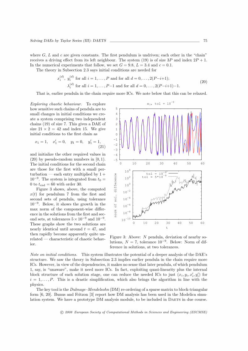
Figure 3: Above: N pendula, deviation of nearby so-lutions, N = 7, tolerance 10−9. Below: Norm of dif-ference in solutions, at two tolerances.

Exploring chaotic behaviour. To explorehow sensitive such chains of pendula are tosmall changes in initial conditions we cre-ate a system comprising two independentchains (19) of size 7. This gives a DAE ofsize 21 × 2 = 42 and index 15. We giveinitial conditions to the first chain as

x1 = 1, x′1 = 0, y1 = 0, y′1 = 1,(21)

and initialize the other required values in(20) by pseudo-random numbers in [0, 1).The initial conditions for the second chainare those for the first with a small per-turbation — each entry multiplied by 1 +10−9. The system is integrated from t0 =0 to tend = 60 with order 30.

Figure 3 shows, above, the computedx(t) for pendulum 7 from the first andsecond sets of pendula, using tolerance10−9. Below, it shows the growth in themax norm of the component-wise differ-ence in the solutions from the first and sec-ond sets, at tolerances 5× 10−9 and 10−9.These graphs show the two solutions arenearly identical until around t = 47, andthen rapidly become apparently quite un-related — characteristic of chaotic behav-ior.

Note on initial conditions. This system illustrates the potential of a deeper analysis of the DAE’sstructure. We saw the theory in Subsection 2.3 implies earlier pendula in the chain require moreICs. However, in view of the dependencies, it makes no sense that later pendula, of which pendulum1, say, is “unaware”, make it need more ICs. In fact, exploiting quasi-linearity plus the internalblock structure of each solution stage, one can reduce the needed ICs to just (xi, yi, x

′i, y′i) for

i = 1, . . . , P . This is a drastic simplification, which also brings the algorithm in line with thephysics.

The key tool is the Dulmage–Mendelsohn (DM) re-ordering of a sparse matrix to block-triangularform [6, 20]. Bunus and Fritzon [3] report how DM analysis has been used in the Modelica simu-lation system. We have a prototype DM analysis module, to be included in Daets in due course.



5.3 A continuation problem

A continuation problem can be viewed as a system of n purely algebraic equations in n+1 variables,f(y) = 0. Generically, the solution is a collection of one-dimensional curves (branches). The taskis to follow a branch from an initial point, in one of the two possible directions, to a desired point.

A typical practical difficulty is “tracking failure”: another branch may come so close that onejumps on to it by mistake. A canonical example (in x, y space, with n = 1) is y2 − x2 = c where cis a small nonzero constant. If one starts in the third quadrant, say near (−1,−1), and continuestoward the origin, one should end up in quadrant 4 if c > 0 or quadrant 2 if c < 0. However, atfixed precision and for small enough c, any numerical method is bound to “miss” the sharp bendnear the origin and end up in quadrant 1. The high-order method used by Daets makes it ratherrobust because it enables it to “see” such bends from quite far off.

Continuation is commonly used to solve hard systems of n equations in n variables, using aparameter to move from a trivial problem to the desired one. We illustrate by the “LW problem”,from Layne Watson [29]. One seeks a fix-point, that is a root of

x = g(x) (22)

for the function g : Rn → Rn where

gi(x) = gi(x1, . . . , xn) = exp(cos(i

n∑

k=1

xk)), i = 1, . . . , n. (23)

Define y = (λ,x) and consider the parameterized problem

0 = f(y) = x− λg(x). (24)

y

x

Figure 4: Typical path shape thatcauses tracking failure.

The idea is to follow the branch through the trivial solutionat y = (λ,x) = (0,0) in the direction of increasing λ until wereach a point with λ = 1, which will solve our problem.

Even for n as small as 10, solving (22) without continuationis not easy, partly because it has many solutions. Continua-tion helps; one benefit is that (24) identifies a specific solution,the unique first one on this continuation path. However, evenfor small n, tracking problems are quite severe.

It is well known that taking λ as the independent vari-able in such problems generally fails because of turning pointswhere dx/dλ is infinite. Instead, we use arc length continua-tion, introducing an independent variable s and adding to (24)

an (n+1)th equation (‖dy/ds‖2)2

= 1 that defines s as Euclid-

ean arc-length along the path. That is 0 = S =∑j y′j2 − 1,

where ′ means d/ds.This formulation gives an index 1 DAE. How does Daets

know which direction to take along the path? The code recognizes the DAE as not quasi-linearand thus requires values xJ≤0

, in the notation of Subsection 2.3, as an initial guess. It turns outthat these values comprise y and y′ — both an initial position, and an initial direction, just whatis needed.

Since Daets currently lacks event location, finding s where λ(s) = 1 was done by putting thecode into one-step mode and, after a step where a sign-change of (λ−1) was observed by the callingprogram, root-finding by a reverse-communication version of Brent’s Zeroin. Figure 5 shows, forn = 10, the graphs of two components x1 and x10 against λ. Many turning points are visible. Thepath in full (λ, x1, . . . , xn) space is convoluted and gets rapidly more so as n increases, as shownby the increasing arc length traversed as λ goes from 0 to 1.



x1, x10

λ

x1x10x1x10

0

0.5

1

1.5

2

2.5

0 0.2 0.4 0.6 0.8 1 1.2 1.4

Figure 5: LW problem, n = 10. Paths of x1 and x10 plot-ted against continuation parameter λ. The markers showsuccessive points computed at the slackest tolerance 0.03 atwhich Daets succeeded. For the curve, tolerance 1e–7 wasused. Points beyond λ = 1 are part of the event location.

Our numerical experiments areabout how robust Daets is on theLW problem as n increases. (i) Doesit manage to reach λ = 1? (ii) Doesit avoid tracking failures?

We did this by solving, for eachn used, with a variety of tolerancesand orders. Having no reference solu-tions, we compared all the vectors x,from those integrations that reachedλ = 1. If there were several such,and they were all essentially equal,we counted them as the correct so-lution. If not, tracking failure hadcertainly occurred.

The first tests used orders p = 0(meaning the code’s default order for-mula), 20, 30, 40, 50 and tolerancesτ = 10−3, 10−5, 10−7, 10−9, 10−11,10−12 with a mixed error test: 30runs for each n. When there was noupper limit on the stepsize h (thatis, it was chosen as described in Sec-tion 3), tracking failures were seen for quite small n. Three solutions were found for n = 4, 6, 9;four for n = 12; six for n = 14; one for all other n up to 20. Every computed solution was a “good”one in that the residual norm ‖x− g(x)‖∞ was under 10−11.

Things improved when we limited the size of h. The constraint h ≤ 0.3 sufficed to ensure thatonly one solution was found for each n we tried. The above 30 combinations (p, τ) were used forn = 1, 2, . . . , 20: just two runs failed “h too small” at the smallest tolerance. For larger n, fewer(p, τ) were used because of the extensive running times; for n = 25, 30, 35, 40 we found only onesolution, though more failures at the smallest, and for a reason still obscure, the largest tolerance.

Since the un-limited h could vary from around 10−8 to around 6, we guess that the pathshave long “easy” stretches, followed by a sudden bend that the code misses if h is un-limited. Ourresults suggest that the risk of tracking failure on the LW problem depends on geometrical featuresspecific to each n, and does not increase steadily with n.

With the h-limit, which makes little difference to overall run times, the evidence is that Daets,used as described, is a robust continuation code.

6 A complete code example

Here is code, self-explanatory in the light of the foregoing, for integrating the one-pendulum ex-ample (8). We omit output. More extensive examples, with output, are in the User Guide [22].

1 #include "DAEsolver.h"

2 template <typename T> void fcn( int n, T t, const T *z, T *f, void *p) {

3 // z [ 0 ] , z [ 1 ] , z [ 2 ] a r e x , y , lambda .4 const double g = 9.8 , L = 10.0;

5 f[0] = Diff(z[0] ,2) + z[0]*z[2];

6 f[1] = Diff(z[1] ,2) + z[1]*z[2] - g;

7 f[2] = sqr (z[0]) + sqr(z[1]) - sqr(L);

8 }



9 int main () {

10 const int n = 3; // s i z e o f the problem11 DAEsolver Solver(n, DAE_FCN(fcn )); // c r e a t e a s o l v e r , a n a l y s e DAE12 Solver.printDAEinfo (); // p r i n t i n f o about the DAE13 Solver.printDAEpointStructure (); // . . and more i n f o14 DAEsolution x(Solver ); // c r e a t e a DAE s o l u t i o n o b j e c t15 x.setT (0.0); // i n i t i a l v a l u e o f t16 x.setX (0 , 0 , -1.0). setX (0 , 1 , 0.0); // . . and o f x and x ’17 x.setX (1 , 0 , 0.0). setX (1 , 1 , 1.0); // . . and o f y and y ’18 double tend = 100.0;

19 DAEexitflag flag;

20 Solver.integrate(x, tend , flag ); // i n t e g r a t e u n t i l tend21 i f (flag != success ) printDAEexitflag(flag );// check the e x i t f l a g22 x.printSolution (); // p r i n t s o l u t i o n23 x.printStats (); // p r i n t i n t e g r a t i o n s t a t i s t i c s24 return 0;

25 }

7 Conclusions

Daets is a DAE solver based on Pryce’s structural analysis (SA) and the use of automatic dif-ferentiation to expand the solution in Taylor series. The code is available from the authors underlicence. We invite people to submit real-life DAE problems for which the Daets approach shouldbe suitable, to help us further develop the capabilities of the code.

Daets has shown itself robust in our experiments. It has as good accuracy-to-tolerance pro-portionality as do the codes Dassl and Radau, and far better on the index 3 car axis problem(Subsection 5.1). It is especially effective at high accuracies. Its symbolic understanding of theDAE structure lets it handle high index problems (Subsection 5.2), as well as purely algebraiccontinuation problems (Subsection 5.3) and explicit or implicit ODEs.

The results of the SA can be printed, which is a help to understanding an unfamiliar DAE. Amethod to find an initial consistent point is built into Daets, in contrast to most solvers.

Daets copes well with moderately stiff problems because of the increasing stability regions ofTaylor methods as the order increases. It cannot handle very large problems, very stiff problems,and those where SA gets the structure wrong. These pose three rather different challenges:

Large problems. The difficulty is mainly practical: the memory requirement of high-order TSmethods and the computational work associated with AD. One can improve this by using sparselinear algebra and by having fewer long vectors active at once while computing Taylor coefficients.This suggests memory management based on a frontal analysis of the computational graph. How-ever, probably no one wants to solve very large problems to the great accuracy that is the mainadvantage of Taylor methods.

Stiff problems. There is a real need to develop SA-based methods with suitable stability. A naturalextension of our approach would be to adapt Hermite-Obreschkoff (HO) methods, which are a sortof Taylor series from both ends of the interval at once. For ODEs they are an effective alternativeto Taylor methods with the extra advantage of handling stiffness [8, 18]. It is an interesting taskin numerical analysis to devise the formulas and data structures to achieve this for DAEs.

Wrong structural analysis. This event is rare in our experience, but will become commoner as SA-based methods are applied to DAEs generated automatically by software for interactive modellingand simulation. It poses another interesting and difficult task, more in computer science than innumerical analysis. In all cases we have seen, we could make SA get the right answer by rearrangingthe DAE, manually, in an equivalent form but with “better sparsity”. What are the principles andmethods involved, and can they be at least partially automated?



References

[1] U. M. Ascher, Hongsheng Chin, and Sebastian Reich. Stabilization of DAEs and invariant manifolds.Numerische Mathematik, 67(2):131–149, 1994.

[2] K. Brenan, S. Campbell, and L. Petzold. Numerical Solution of Initial-Value Problems in Differential-Algebraic Equations. SIAM, Philadelphia, second edition, 1996.

[3] P. Bunus and P. Fritzon. Methods for structural analysis and debugging of Modelica models. InProceedings of the 2nd International Modelica Conference, pages 157–165. Deutsches Zentrum furLuft und Raumfahrt Oberpfaffenhofen, Germany, March 2002.

[4] S. L. Campbell and C. W. Gear. The index of general nonlinear DAEs. Numerische Mathematik,72:173–196, 1995.

[5] Y. F. Chang and George F. Corliss. ATOMFT: Solving ODEs and DAEs using Taylor series. Comp.Math. Appl., 28:209–233, 1994.

[6] A. L. Dulmage and N. S. Mendelsohn. Coverings of bipartite graphs. Canad. J. Math, 1958.

[7] A. Griewank, D. Juedes, and J. Utke. ADOL-C, a package for the automatic differentiation of algo-rithms written in C/C++. ACM Trans. Math. Software, 22(2):131–167, June 1996.

[8] E. Hairer, S. P. Nørsett, and G. Wanner. Solving Ordinary Differential Equations I. Nonstiff Problems.Springer-Verlag, second edition, 1991.

[9] E. Hairer and G. Wanner. Solving Ordinary Differential Equations II. Stiff and Differential– AlgebraicProblems. Springer Verlag, Berlin, 1991.

[10] T. E. Hull and W. H. Enright. A structure for programs that solve ordinary differential equations.Technical Report 66, Department of Computer Science, University of Toronto, May 1974.

[11] R. Jonker and A. Volgenant. A shortest augmenting path algorithm for dense and sparse lin-ear assignment problems. Computing, 38:325–340, 1987. The assignment code is available atwww.magiclogic.com/assignment.html.

[12] A. Jorba and M. Zou. A software package for the numerical integration of ODEs by means of high-order Taylor methods. Technical report, Department of Mathematics, University of Texas at Austin,TX 78712-1082, USA, 2001.

[13] S. E. Mattsson and G. Soderlind. Index reduction in differential-algebraic equations using dummyderivatives. SIAM J. Sci. Comput., 14(3):677–692, 1993.

[14] F. Mazzia and F. Iavernaro. Test set for initial value problem solvers. Technical Report 40, Departmentof Mathematics, University of Bari, Italy, 2003. http://pitagora.dm.uniba.it/∼testset/.

[15] N. S. Nedialkov and K. R. Jackson. The design and implementation of a validated object-orientedsolver for IVPs for ODEs. Technical Report 6, Software Quality Research Laboratory, Department ofComputing and Software, McMaster University, Hamilton, Canada, L8S 4K1, 2002.

[16] N. S. Nedialkov and J. D. Pryce. Solving differential-algebraic equations by Taylor series (I): Com-puting Taylor coefficients. BIT, 45:561–591, 2005.

[17] N. S. Nedialkov and J. D. Pryce. Solving differential-algebraic equations by Taylor series (III):The DAETS code. Technical report, Department of Computing and Software, McMaster University,Hamilton, Ontario, Canada, L8S 4K1, November 2007.

[18] N. S. Nedialkov. Computing Rigorous Bounds on the Solution of an Initial Value Problem for anOrdinary Differential Equation. PhD thesis, Department of Computer Science, University of Toronto,Toronto, Canada, M5S 3G4, February 1999.

[19] C. C. Pantelides. The consistent initialization of differential-algebraic systems. SIAM. J. Sci. Stat.Comput., 9:213–231, 1988.

[20] A. Pothen and C.-J. Fan. Computing the block triangular form of a sparse matrix. ACM Transactionson Mathematical Software, 16(4):303–324, December 1990.

[21] LAPACK project. LAPACK — Linear Algebra PACKage. http://www.netlib.org/lapack/.



[22] J. D. Pryce and N. S. Nedialkov. DAETS user guide. Technical report, Department of Computingand Software, McMaster University, Hamilton, Ontario, Canada, L8S 4K1, 2007.

[23] J. D. Pryce. Solving high-index DAEs by Taylor Series. Numerical Algorithms, 19:195–211, 1998.

[24] J. D. Pryce. A simple structural analysis method for DAEs. BIT, 41(2):364–394, 2001.

[25] G. J. Reid, P. Lin, and A. D. Wittkopf. Differential-elimination completion algorithms for DAE andPDAE. Studies in Applied Mathematics, 106(1):1–45, December 2001.

[26] G. Reissig, W. S. Martinson, and P. I. Barton. Differential–algebraic equations of index 1 may havean arbitrarily high structural index. SIAM J. Sci. Comput., 21(6):1987–1990, 1999.

[27] O. Stauning and C. Bendtsen. FADBAD++ web page, May 2003. FADBAD++ is available atwww.imm.dtu.dk/fadbad.html.

[28] A. Wachter. An Interior Point Algorithm for Large-Scale Nonlinear Optimization with Applicationsin Process Engineering. PhD thesis, Carnegie Mellon University, Pittsburgh, PA, 2002.

[29] L. T. Watson. A globally convergent algorithm for computing fixed points of C2 maps. Appl. Math.Comput., 5:297–311, 1979.


solving di erential algebraic equations by taylor series … (that is, enclosures of the solutions)...

Documents