Solving Real-World Cutting Stock-Problems

in the Paper Industry– Mathematical Approaches, Experience and Challenges –

Julia Kallratha,b, Steffen Rebennackc,∗, Josef Kallrathd, Rudiger Kuschee

aGSEmbH, Oranienpassage 1, 57258 Freudenberg, Germanybh da Hochschule Darmstadt, Schofferstr. 3, 64295 Darmstadt, Germany

cColorado School of Mines, Division of Economics and Business, Golden, CO 80401, USAdUniversity of Florida, Dept. of Astronomy, Gainesville, FL 32611, USA

eGSEmbH, Oranienpassage 1, 57258 Freudenberg, Germany

Abstract

We discuss cutting stock problems (CSPs) from the perspective of the paper industry and the financial impactthey make. Exact solution approaches and heuristics have been used for decades to support cutting stockdecisions in that industry. We have developed polylithic solution techniques integrated in our ERP system tosolve a variety of cutting stock problems occurring in real world problems. Among them is the simultaneousminimization of the number of rolls and the number of patterns while not allowing any overproduction. Fortwo cases, CSPs minimizing underproduction and CSPs with master rolls of different widths and availability,we have developed new column generation approaches. The methods are numerically tested using real worlddata instances. An assembly of current solved and unsolved standard and non-standard CSPs at the forefrontof research are put in perspective.

Keywords: paper industry, cutting stock, roll production, format production, column generation, columnenumeration, operations research, stochastic demand, real-world optimization

1. Introduction

The pulp and paper industry plays an importantrole worldwide. There are in the order of 3000 pa-per mills, which produced a total of 394 milliontons of paper and paperboard, in 2010. Europe (in-cluding Russia) has approximately 900 paper mills,while Germany has about 180. The largest pro-ducer in the world is the Finnish UPM group withan annual tonnage of 12.7 million tonnes, followedby Stora Enso with 11.8 million tons and by In-ternational Paper with 9.7 million tonnes per year.Santos and Almada-Lobo (2012) report that in Por-tugal the pulp and paper industry contributes over

∗Corresponding authorEmail addresses: julia.kallrath@h-da.de (Julia

Kallrath), srebenna@mines.edu (Steffen Rebennack),kallrath@astro.ufl.edu (Josef Kallrath),ruediger.kusche@gse-software.de (Rudiger Kusche)

URL: http://www.fbmn.h-da.de/~kallrath/ (JuliaKallrath), http://www.rebennack.net (Steffen Rebennack),http://astro.ufl.edu/~kallrath (Josef Kallrath)

4% of the GDP and 5% of the active employees. Asit is subject of both local and global environmen-tal discussions, effective planning and cutting stocktechniques lies at the very heart of the operationalperformance of its manufacturing organizations.

Exact solution approaches and heuristics havebeen used for decades to support cutting stock deci-sions in the paper industry. In the standard cuttingstock problem (CSP), the problem input is given bya set of item sizes and demands, and by a set of mas-ter rolls of given widths; the simplest case consistsof only one type of master rolls. The task is to de-cide on how many master rolls are cut to a certainpattern in order to minimize the total number ofmaster rolls used.

The pattern minimization problem (PMP) is astrongly NP-hard cutting problem, which seeks acutting plan with the minimum number of differ-ent patterns, cf. McDiarmid (1999). This objec-tive, relevant when changing from one pattern toanother, involves a cost for setting up the cutting

Preprint submitted to European Journal of Operational Research December 4, 2013

machine, i.e., adjusting the cutting knifes. Whenthe minimization of the number of different pat-terns is done by assuming that no more than theminimum number of rolls can be used, the problemis also referred to as the cutting stock problem withsetup costs.The international working group SICUP (Special

Interest Group on Cutting and Packing) founded byGerhard Wascher in 1988, focuses on cutting stockand packing problems and is a platform for morethan 200 practitioners and scientists to exchangeideas on these topics. In 2004, SICUP became theEURO working group ESICUP (EURO Special In-terest Group on Cutting and Packing).The main contributions of this paper can be clas-

sified into two categories:

Mathematical optimization: For 1D CSPs withtwo criteria, minimizing the number of rollsand the number of patterns, we develop an Ex-haustion Method (Sect. 3.4), a column genera-tion approach allowing underproduction (Sect.3.5.4) and column generation approach incor-porating master rolls with different widths andlimited availability (Sect. 3.5.5). We presenta novel polylithic1 solution method towards2D trim-loss minimization (Sect. 4). Further-more, we share real data in a 1D cutting stockbenchmark data set (Sect. 3.6.1). For softwareproducts, it is not untypical to combine var-ious basic algorithms to consistently providesolutions in acceptable time, with many em-pirical rules, or even rules of thumb, to decidewhich algorithms to use in each circumstance.We disclose this information instead of keepingit as a commercial secret, to provide evidencethat there is more exact optimization and lessheuristics involved as one might expect.

Managerial insights for the paper industry:We present real-world aspects relevant to thepaper industry, which have seen only littletreatment in the scientific literature (Sect.3.5). We assemble current cutting-edgestandard and non-standard cutting stockproblems relevant to the paper industry (Sect.

1The term polylithic has been coined by Kallrath (2009a)and explained in greater detail in Kallrath (2011); it refersto modeling and solution approaches in which mixed integeror nonconvex nonlinear optimization problems are solved bytailor-made methods involving several models and/or solvestatements or algorithmic components.

5) and illuminate at length the variants andissues present in real-world problems. Wediscuss the financial impact mathematicalprogramming-based solutions to cutting stockproblems have in the paper industry (Sect. 6).

The remainder of the paper is structured as fol-lows: After a literature review in Section 2, we dis-cuss the 1D CSP and its variants in Section 3 alongwith different solution techniques. A presentationof 2D polylithic solution methods in Section 4 is fol-lowed by a discussion of current-edge CSPs in Sec-tion 5 and our views on optimization in the paperindustry in Section 6. Conclusions are in Section7. Two appendices, post-processing (Appendix A)and guidelines on how to derive the pricing prob-lems (Appendix B) complete this paper.

2. Literature Review

There is a rich body of literature available onCSPs; cf. Haessler and Sweeney (1991) andHaessler (1992) for reviews on 1D cutting stockproblems and solution procedures. We find heuris-tic solution approaches (cf. Haessler (1971)), exactMILP-models (cf. Johnston and Sadinlija (2004)),column generation approaches, among them theclassical paper by Gilmore and Gomory (1961),Branch&Price algorithms (cf. Belov and Schei-thauer (2006)), reviews as by Amor (2005) who putcolumn generation and Branch&Price algorithms inperspective, and classification papers (cf. Dyckhoff(1990) and Wascher et al. (2007)).Most of the approaches described in the literature

for solving the PMP are based on heuristics. As thePMP has been proven strongly NP-hard by McDi-armid (1999), it is not a surprise that solving theproblem exactly has been a real challenge, and onlyvery few exact solution methods have been reportedso far in the literature; among them Vanderbeck(2000). Alves et al. (2009) explore an integer pro-gramming model that can be solved using columngeneration, and they describe different strategies tostrengthen it, among which are constraint program-ming and new families of valid inequalities. Lowerbounds for the pattern minimization problem arederived from the new integer programming model,and also from a constraint programming model.Beyond a vast body of literature on the stan-

dard CSP, there are a few publications on a gen-eralized CSP with great practical significance: Themultiple-width CSP with master rolls of different

2

widths (and equal lengths assumed to be infinite).An early work on this topic is by Holthaus (2002),who solves the relaxation of the CSP by the columngeneration technique and uses three procedures forrounding the solution, leading in a final residualproblem, which is solved by an ILP-solver. Al-though his technique is suitable for solving medium-size and large instances of the one-dimensional CSP,the paper does not consider supply limitation onthe different stock lengths availability. Alves andde Carvalho (2007) developed strategies to stabi-lize and accelerate the column generation methodby introducing dual-optimal inequalities, reducingthe number of column generation iterations and runtime. Finally, Poldi and Arenales (2009) providea heuristic to solve the CSP with multiple stocklengths with limited availability.Although production planning or scheduling and

CSPs are usually treated separately, we find earlyarticles in which both aspects are combined; cf.Haessler and Talbot (1983) or Li (1996) who pro-vide LP-based and non-LP-based heuristics to solve2D multi-job cutting stock problems with due datesand release dates. The combined cutting stock andlot-sizing problem in industrial processes has at-tracted several authors in the last decade, amongthem Arbib and Marinelli (2005), Gramani andFranca (2006), Yanasse and Pinto Lamosa (2007),Trkman and Gradisar (2007), Poltroniere et al.(2008), Gramani et al. (2009) and most recentlyReinertsen and Vossen (2010) who treat the 1DCSP with due dates. Trkman et al. (2009) treat cut-ting stock as a continuous business process whichis incorporated into an entire supply chain.General cutting and packing problems are related

to CSPs. The most important difference betweencutting and packing problems is that in cuttingproblems, the number of objects are given and thetask is to minimize trim-loss or area, while pack-ing problems aim to fit as many objects as possiblein a predefined area or volume. For example, onemay want to cut orientation free polygons (Kall-rath, 2009b) or ellipses (Kallrath and Rebennack,2014) into one rectangle, or circles into several rect-angles (Rebennack et al., 2009). A significant dif-ference between these cutting problems cited andthe 2D cutting problems described in Section 4 isthat the latter allow only a horizontal or verticalorientation of the objects to be cut.We conclude our literature review by pointing

the reader to a few articles which give some excel-lent insights into the field: Rodrıguez and Vecchi-

etti (2008) for practical application with very goodillustrations, and similarities to our 2D problem de-scribed in Section 4, Harjunkoski et al. (1998) andPorn et al. (1999) for exact MILP and MINLP ap-proaches, and also, a very recent paper on heuristicsby Cui and Zhao (2013).

3. 1D Cutting Stock Problem

Our discussion of the one-dimensional cuttingstock problem starts with the standard problemformulation in Section 3.1, followed by three solu-tion methods: the widely used approach by Gilmore& Gomory (Sect. 3.2), a column enumeration(Sect. 3.3), and an Exhaustion Method (Sect.3.4). We summarize important practical aspectsfor one-dimensional CSPs for the paper industryand present extensions to the column generationapproach addressing these practical aspects (Sect.3.5). We conclude this section with some computa-tional benchmarking (Sect. 3.6).

3.1. The Standard Problem and its Mathematics

The mathematical model for minimizing thenumber of rolls or trim-loss in the standard problemwith one master roll of width B is characterized bythe following indices, data and variables.

3.1.1. Indices

p ∈ P := {p1, . . . , pNP} cutting patterns; NP isthe number of patterns in P . If NP is notknown, as it happens in the Gilmore and Go-mory approach, we set NP to a sufficientlylarge number.

i ∈ I := {i1, . . . , iN I} given orders or widths; N I

is the number of (orders) widths in I.

3.1.2. Input Data

B [L] width of the master rolls (raw materialrolls).

Di [-] demand; the requested number of pieces ofwidth i.

Wi [L] width of order type i.

3.1.3. Integer Variables

µp ∈ IN0 := {0, 1, 2, 3, . . .} [−] indicates how of-ten pattern p is used; µp = 0 if p is not used.

αip ∈ IN0 [−] indicates how often order type i iscontained in pattern p; 0 ≤ αip ≤ Di.

3

3.1.4. Mathematical Programming Model Formula-tion

A suitable objective function

z∗ := minαip,µp

∑

i∈I

∑

p∈P

f(αip, µp) , (1)

is subject to the restrictions (fulfillment of the de-mand)

∑

p∈P

αipµp = Di , ∀i , (2)

feasibility of pattern p∑

i∈I

Wiαip ≤ B , ∀p , (3)

and the integrality constraints

αip ∈ IN0 , ∀{ip} (4)

and

µp ∈ IN0 , ∀p . (5)

Formulated via (1)-(5), the standard CSP is amixed integer nonlinear (nonconvex) optimizationproblem (MINLP), a problem class which is diffi-cult in itself. As the problem may easily encounterseveral million variables αip, it cannot be solved ef-ficiently in this form. Another complication resultsfrom equation (2) with exact demand fulfillment,as it is rare to find feasible solutions to the CSP.Therefore, in practical situations, (2) is relaxed to

DLi ≤

∑

p∈P

αipµp ≤ DUi , ∀i , (6)

with lower and upper bounds, DLi and DU

i , on thedemand Di. Usually, underproduction is less ac-cepted as light overproduction; see also the discus-sion in Section 3.5.4.

3.2. Gilmore & Gomory Approach (GGA)

The idea of column generation by Gilmore andGomory (1961) is to dynamically add variables(“columns”) which are good candidates to be in-cluded in an optimal solution. This is achieved bydecomposing the CSP into a master problem (MP)and a sub-problem (SP), also called pricing prob-lem. For a predefined set of patterns P ′ ⊆ P , theMP decides how often each pattern has to be usedand provides input data for the SP via dual infor-mation. It minimizes the number of rolls

minµp

∑

p∈P′

µp , (7)

with the demand-fulfill inequalities (note that it isallowed to produce more than requested)

∑

p∈P′

Nipµp ≥ Di , ∀i , (8)

where Nip is the number of times order i is con-tained in pattern p ∈ P ′. The integrality con-straints

µp ∈ IN0 , ∀p ∈ P ′ . (9)

complete the model. Replacing the integrality re-quirement (9) on µp by a non-negative constraint,we obtain the so-called relaxed master problem(RMP).In the SP, new patterns (variables αi, the multi-

plicity of width i) are calculated by exploiting thedual values πi (pricing information) of the RMPassociated with (8). The objective function

minαi

(

1−∑

i∈I

πiαi

)

,

involves the integer variables αi. To ensure that, inthe new pattern, the roll width, B, and the number,K, of knives are not exceeded we add the knapsackinequalities

∑

i∈I

Wiαi ≤ B ,∑

i∈I

αi ≤ K . (10)

Numerical experiments without the knife constraintare indicated byK = ∞. For completeness, we notethe integrality conditions

αi ∈ IN0 , ∀i . (11)

The αi become the Nip coefficients of the new pat-tern in (8). In some cases, αi could be additionallybounded, for instance, by the number, K, of avail-able knives, or by the demand, Di.Once the optimal objective function value of the

SP is non-negative, then the RMP for pattern setP ′ has been solved to optimality over all possiblepatterns. The optimal objective function value ofthe RMP provides a lower bound on z∗; solving theMP for the available set of patterns P ′ yields anupper bound on z∗.In this context, the absolute difference (i.e., gap)

between the RMP and the MP, once GGA con-verges, is of great interest. A well known conjecturestates that the 1D cutting stock problem (whenminimizing the number of patterns used) has theso-called modified round-up property, i.e., the gap

4

is at most 2, cf. Scheithauer and Terno (1995). Noinstance of the 1D cutting stock problem has beenreported so far which has a greater gap. To thebest knowledge of the authors, the conjecture hasnot been proven, yet.

3.3. Column Enumeration

As the expression “column enumeration” (CE)suggests, the set of possible columns (e.g., patterns)is enumerated. As such, CE is a special variant ofcolumn generation and is applicable when a smallnumber of columns is sufficient. For instance, this isthe case in real-world cutting stock problems whenit is known that the optimal solutions have only asmall amount of trim-loss, eliminating most of thepatterns. CE naturally leads to a type of select-ing columns or partitioning models: problem (7)-(9) with P ′ being the set of all generated columns.Despite the limitations with respect to the numberof columns, CE has some advantages: No pricingproblem, easily applicable to MILP problems, mucheasier to implement (compared to column genera-tion), and allows the straight forward incorporationof demand stochasticities (cf. Sect. 5.1). In thecontext of cutting stock problems, we sometimescan use the maximum permissible trim-loss to re-strict the number of patterns to be considered inCE (cf. Sect. 3.5).

3.4. An Exhaustion Method

This method combines a constructive heuristicwith exact MILP techniques. We illustrate theexhausting method by the CSP described in Sec-tion 3.1; assigning orders in a scheduling problemwould be another example of an exhaustion ap-proach. The elegant GGA is known for produc-ing minimal trim-loss solutions withmany patterns.Often this corresponds to setup changes on the ma-chine and therefore is not desirable. A solutionwith a minimal number of patterns minimizes themachine setup costs of the cutter. Minimizing si-multaneously trim-loss and the number of patternsis possible for small cases of a few orders only, ex-ploiting the MILP model by Johnston and Sadinlija(2004). It contains two conflicting objective func-tions. Therefore one could resort to goal program-ming. Alternatively, we produce a pool of severalparameterized solutions leading to different numberof rolls to be used and patterns to be cut from. Itis up to the user to choose the best solution fromthat pool; cf. Section 3.6.4.

Note that the Branch&Price algorithm describedin Vanderbeck (2000) or Belov and Scheithauer(2006) can be used to solve the 1D CSP with mini-mal numbers of patterns. However, these methodsare not easy to implement. Therefore, dependingon the number of orders, we use the following ap-proaches:

• V1: Direct usage of the model by Johnston andSadinlija (2004), for a small number of orders,e.g., N I ≤ 14 and Dmax ≤ 10, to minimize thenumber of patterns or the number of rolls. In apreprocessing step, we compute valid inequal-ities as well as tight lower and upper boundson the variables.

• V2: Exhaustion procedure in which we coverthe orders and their demands by generatingsuccessively new patterns with maximal mul-tiplicities (phase V2-1). If only a small num-ber of orders is left over, we use V1 to minimizethe number of rolls (phase V2-2). In phase V2-3, we exploit the MIPSTART feature of CPLEX

and start with the best solution found (small-est number of patterns) and use again V1 tominimize the number of patterns with the aimto compute an improved lower bound, NP

2−,smaller than our initial lower bound, NP

1−,which we obtained by solving the correspond-ing bin packing problem (BPP, resulting fromsetting all CSP demands to 1), and to find abetter solution.

3.4.1. Indices and Sets

In this model, we use the indices listed in John-ston and Sadinlija (2004):

i ∈ I := {i1, . . . , iN I} the index set of (order)widths.

p ∈ P := {p1, . . . , pNP} the set of all possible pat-terns; NP ≤ N I. The patterns are generatedby V1, or dynamically by maximizing the mul-tiplicities of a pattern used. Note that in John-ston and Sadinlija (2004), the index j is usedinstead of p.

k ∈ K := {k1, . . . , kNK} the multiplicity index toindicate how often a width is used in a pattern.The multiplicity index can be bounded by theratio of the widths of the orders and given rolls.

5

3.4.2. Variables

The following integer or binary variables areused:

αip ∈ IN [−] specifies how often width i occursin pattern p; 0 ≤ αip ≤ Di (item–in-patternmultiplicity).

αipk ∈ IN [−] auxiliary variable connected toδipk; 0 ≤ αipk ≤ Dmax := maxi Di.

δAp ∈ {0, 1} [−] indicates whether pattern p isused at all.

δipk ∈ {0, 1} [−] indicates whether width i ap-pears in pattern p at level k; δipk = 0 impliesaipk = 0.

µp ∈ IN [−] specifies how often pattern p is used.If pattern p is not used, we have µp = δAp = 0.

3.4.3. The Idea of the Exhaustion Method

In our exhaustion procedure, we cover the or-ders and their demands by generating successivelynew patterns with maximal multiplicities. If only asmall number of orders is left over, we switch to V1.This method is parameterized by the initial per-missible percentage waste Wmax, 1 ≤ Wmax ≤ 99.To populate the pool, we use six parameterizationswith the following values: Wmax = 20, 15, 10, 8,6 and 4. The usage of different parametrizations ismotivated by the hope to obtain different solutions.This allows the user to select the best combinationof number of rolls and number of patterns.We start with iteration m = 0. In each iteration

m, we generate at most 2 new patterns by maximiz-ing the multiplicities of these patterns allowing nomore than a maximum percentage waste,Wmax, rel-ative to the width of the master roll. The solutiongenerated in iteration m is preserved in iterationm + 1 by fixing the appropriate variables. If theproblem turns out to be infeasible (this may hap-pen if Wmax turns out to be restrictive; we observedthis to happen occasionally for Wmax < 8), we in-crease the permissible waste by 10% and proceedto the next iteration. If only a few orders remain,we switch to V1 to cover the remaining unsatisfiedorders; note that V1 works without the Wmax re-striction.Our model is based on the MILP model devel-

oped by Johnston and Sadinlija for solving the1D-CSP problem, especially on their inequalities(1,2,3,5-8). Their main idea is to replace the nonlin-ear terms in (2) by binary variables δipk, which take

value 1 if item i occurs in pattern p with multiplic-ity k. Similar transformations have been presentedbefore by Harjunkoski et al. (1998). The model byJohnston and Sadinlija can work efficiently, if we ex-pect to have only reasonably small item-in-patternmultiplicities k and not too many items and pat-terns.

It helps, and is also necessary, to provide lowerand upper bounds, NP

− and NP+ , on the number of

patterns expected to be used in an optimal solution.If N I is the number of items (order widths), thenNP

1+ := N I is a weak upper bound. We computea weak lower bound, NP

1−, by applying the GGAtowards a BPP associated with the CSP problem.

The great strength of the model by Johnston andSadinlija is that it allow us to implement differ-ent objective functions and constraints much easierthan in a MINLP model or in column generationapproaches. Therefore, it even allows for sequenc-ing production by exploiting a one-to-one corre-spondence between pattern and manufacturing se-quence. We briefly summarize the relevant relationswe implemented in our exhaustion; note that wepartially adjusted the nomenclature used by John-ston and Sadinlija to be consistent with our paper.

Let binary variable δAp indicating whether or notpattern p ∈ P is used in the optimal solution. Thepattern multiplicity, µp, is subject to lower and up-per bounds, ML and MU, i.e.,

µp ≥ ML , p ∈ Pact := {1, . . . , NP−} (12)

and (p ∈ Ppot := {NP− + 1, . . . , NP

+})

MLδAp ≤ µp ≤ MUδAp . (13)

Johnston and Sadinlija leave it to the user to setML and MU. Setting ML = 1 is the easiest choice;we use MU = maxi{Di}.

The binary variables δipk are accompanied by in-teger variables αipk which are constructed in sucha way that δipk = 1 implies αipk = µp. Instead ofa fixed demand Di, Johnston and Sadinlija allowfor bounded under- and overproduction, i.e., DL

i ≤Di ≤ DU

i , and thus

DLi ≤

∑

p

∑

k

kαipk ≤ DUi , ∀i . (14)

The various binary and integer variables δipk, αipk,

6

and µp are connected by

αipk ≤ MUδipk , ∀{ipk} , (15)∑

k

δipk ≤ 1 , ∀{ip} , (16)

∑

k

αipk ≤ µp , ∀{ip} , (17)

and

MU∑

k

δipk −∑

k

αipk + µp ≤ MU , ∀{ip} .

(18)Inequalities (15) and (16) guarantee that only oneδipk and its corresponding αipk can be selected foreach pair (ip). Inequalities (17) and (18) guaranteethat αipk > 0 implies αipk = µp.The proper design of the patterns is ruled by the

knapsack inequalities∑

i

∑

k

Wikδipk ≤ B , ∀p , (19)

and∑

i

∑

k

Wikδipk ≥100−Wmax

100B , ∀p . (20)

We add additional constraints to the model, e.g.,the symmetry breaking inequality

δAp ≥ δAp+1 , ∀p , (21)

which ensures that pattern p + 1 can only be usedif p is used. The symmetry breaking inequality

µp ≥ µp+1 , ∀p , (22)

orders the patterns according to their multiplicities.We exploit the Johnston and Sadinlija model by

three objective functions. In V2-1, we maximize themultiplicities of the patterns generated

maxµp

∑

p∈Ppot

µp ,

while in (14) we set DLi = 0 and DU

i = D′i, where

D′i is the number of remaining orders of width index

i. In V1, we minimize the number of patterns

NP := minδp

∑

p∈P′

δp = PL +minδAp

∑

p∈Ppot

δAp ,

subject to DLi = DU

i = Di, and in V2-2, we mini-mize the number of rolls

minµp

∑

p∈Ppot

µp (23)

subject to DLi = DU

i = Di. The model is completedby the integrality conditions (∀{ik} and p ∈ Ppot)

µp, αipk ∈ IN0 , δAp , δipk ∈ {0, 1} .

The model is applied several times with αipk ≤ D′i.

Especially, the model has to fulfill the relationships(∀{ik} and p ∈ P ′)

kαipk > D′i =⇒ αipk = 0 ∧ δipk = 0

as well as (∀{ik} and p ∈ Ppot)

αipk ≤

⌈

D′i

k

⌉

and αipk ≤

⌈

D′i + Si

k

⌉

,

where Si denotes the permissible overproduction.This Exhaustion Method provides an improved

upper bound, NP2+ = NP

min, NP2+ ≤ NP

1+, on thenumber of patterns, where NP

min is the number ofpatterns in the best solution (smallest number ofpatterns) of the pool.

3.4.4. Phase V2-3: Computing the Lower Bound onthe Number of Patterns

To compute a lower bound on NP−, we apply two

methods. The first method is to solve a BPP whichis equivalent to minimizing the number of rolls inthe original cutting stock problem described in Sec-tion 3.1 for equal demands Di = 1. If solved withthe column generation approach, this method is fastand cheap (for the cases we are interested in withup to 80 orders), but the lower bound, NP

1−, ob-tained is often weak for the PMP, cf. Vanderbeck(2000)). The second method, used in phase V2-3, is to exploit the NP

min solution to use the exactmodel V1 for minimizing the number of patterns.This enables us to work with a smaller set of po-tential patterns Ppot = {1, . . . , NP

min}. It is im-pressive to see how quickly the commercial solversCPLEX and XpressMP improve upon the lower boundyieldingNP

2−, when we utilize the MIPSTART feature.For most examples with up to 50 orders we obtainNP

2+−NP2− ≤ 2, but in many casesNP

2+−NP2− = 1 or

evenNP2+ = NP

2−. Sometimes, in step V2-3, we evenfind a better solution, i.e., a solution with fewerpatterns than NP

min.

3.5. Practical Aspects in the Paper Industry: To-wards an Implementation at GSEmbH

Production in the paper industry is closely con-nected to the cutting machines and their properties,e.g., the number of available knifes, or the minimal

7

distance to the edges of the master rolls. The pro-duction philosophy in each company differs. Usu-ally, the production planning problem and the cut-ting stock problem are not treated in one consis-tent MILP or MINLP model. As these two prob-lems are inseparable, they must be solved somehowhand-in-hand, if not in one algorithm then at leastiteratively. In some production planning heuristics,groups of orders are constructed, which become theinput of a CSP. However, it is not unusual to findpeople working out the cutting stock pattern toleave out a few orders as they do not ideally fit intothe patterns constructed or lead to patterns withtoo much trim-loss. These missing orders are con-sidered in later production runs. In the strict sense,this means that underproduction is allowed. Whilethe GGA in its standard form assumes that overpro-duction is allowed, in many practical instances, theplanners are not amused about overproduction anddo not really know what to do with the additionalitems. Efficient patterns with only a few percenttrim-loss are an important issue which can easilyconflict with other objectives, e.g., to minimize thenumber of patterns used. All these practical issuesrequire us to apply modifications to the GGA or toresort to other techniques.

3.5.1. Implementing the Gilmore & Gomory Col-umn Generation Approach

The GGA requires a few modifications to avoidthe production of unnecessarily many orders:

• Generation of the initial patterns (by solvinga separate knapsack problem which maximizesthe number of used widths in the pattern whileensuring that each width is used at most twicei.e., αi ≤ 2, ∀i). If it is desirable to work pri-marily with efficient patterns, then it is bet-ter not to restrict αi artificially but only usethe demand, Di, for item i, in the inequalityαi ≤ Di, ∀i, in order to fill the patterns tothe maximum. The initial knapsack problemis solved N I times. To guarantee feasibility ofthe initial master problem, we enforce for the i-th problem that width Wi is contained at leastonce in the pattern.

• When dynamically generating new patterns,we ensure that each width is not containedmore often than it is ordered. However, thisrestriction cannot be used when only efficientpatterns with the minimum waste are consid-ered.

• Post-processing: Elimination of surplus itemsgenerated by the GGA as described in Ap-pendix A.

Additional constraints lead to an extension of theGGA approach, which we refer generally to as col-umn generation approach (CGA). These constraintsmay enter the master problems and/or the pric-ing problems. Constraints which influence the pat-tern design show up in the pricing problem. Therestriction of the number of knives is one exam-ple. Another example is the requirement that verysmall strips need to be embedded by normal or-der widths. As long as such constraints do not re-quire substantially more effort to solve the pricingproblems they are harmless, i.e., the additional con-straints do not destroy the structure of the pricingproblems. Constraints showing up in the masterproblem tend to produce more difficulties. An ex-ample are constraints counting and restricting thenumber of patterns used in the optimal minimaltrim-loss solution. We discuss two additional ex-amples and their mathematics in Sections 3.5.4 and3.5.5.In general, we observe that the pattern space gen-

erated by the GGA is not complete. Thus, usingthe generated patterns by the GGA approach andchanging the objective function or imposing addi-tional constraints may lead to sub-optimal solutionsor an infeasible problem.If the CGA, due to additional constraints or a

modified objective function, does not work effi-ciently anymore, we resort to complete or partialcolumn enumeration in which we construct reason-able patterns explicitly. Afterwards, a set parti-tioning problem is solved for a different objectivefunction. However, this approach works only if nottoo many patterns are generated (in the order of 104

to 5 ·104); otherwise, it may become too difficult tosolve the partitioning problem.

3.5.2. Efficient Patterns

The paper producers very often want to acceptonly efficient patterns which do not have more thana certain trim-loss, Wmax, derived from the toler-able percent trim-loss, W%

max. Depending on theorder situation, this constraint may lead to infea-sible situations. This is illustrated by the follow-ing example (all data carry the same units): Amaster roll with width of W = 266, and orderwidths W1 = 140, W2 = 138, and W3 = 136lead to patterns with only one order width. This

8

in turn produces an unacceptable large strip-lossof (266 − 140)/266 = 47.36%. Thus, for W%

max

≤ 47.36%, the problem becomes infeasible.In such cases, it is helpful to derive the smallest

value, W%min, of W

%max for which a feasible solution

exists at all. What happens in real life is that theplanner changes the order spectrum to leave out oneor several critical orders. Again, this selection canbe supported by appropriate auxiliary models. Weallow underproduction with respect to the given or-ders but our objective function is to minimize thisunderproduction. In order to achieve this, we gen-erate the patterns by the GGA, followed by a mas-ter problem in which we minimize the underproduc-tion. A conceptual problem with this approach isthat we cannot be sure that we really produced allrelevant patterns. Thus, we only obtain an upperbound on underproduction.

3.5.3. Exact Demand Satisfaction

The demand is usually not met exactly with theGGA, as the column generation can lead to over-production. In cases, in which we apply the GGA,we eliminate superfluous orders where possible withthe heuristics described in Appendix A. How-ever, these simple heuristics cannot always elimi-nate overproduction. In these cases, we resort tothe MILP model of Johnston and Sadinlija to com-pute exact demand solutions.The simple inequality (∀i and p ∈ P ′)

Nip ≤ Di

in the pricing problem can avoid some overproduc-tion problems. If the initial patterns also obey thisinequality, at least, it is impossible that the usageof a single pattern p with µp = 1 exceeds demand.Partitioning models adhere to the following up-

per bound on µp

µp ≤ maxi | Nip>0

{⌈

Di

Nip

⌉}

, ∀p ∈ P ′ .

This is, however, rather a numerical improvementwhen solving the master problem and does notstrictly avoid overproduction. Adding the follow-ing upper bound on µp

µp ≤ mini | Nip>0

{⌊

Di

Nip

⌋}

, ∀p ∈ P ′

to the partitioning model may help, but can easilylead to infeasibility.

One might feel tempted to avoid overproductionby solving the CGA master problem with the exactdemand constraint

∑

p∈P′

Npiµp = Di , ∀i ,

replacing (8). Unfortunately, this may also lead toan infeasible partitioning problem as the patternspace does not allow for this. The resulting GGAstill converges theoretically. However, besides fea-sibility issues when solving the master problem, thegap might no longer be small.The fundamental problem with exact demand

fulfillment is to generate the correct pattern space.A Branch&Price procedure is able to achieve thisbut at significant effort, computationally as well asimplementation wise. For completeness, we notethat if overproduction is allowed, then (p ∈ P ′)

B −∑

i∈I

Nip ≤ mini

Di .

3.5.4. Allowing Underproduction

In real-world CSPs, we experience at least tworeasons for allowing or dealing with underproduc-tion. The first reason is, that the group of orderscould lead to patterns which are not easily accepteddue to large trim-loss. People prefer to leave outsome complicating orders or to fulfill them only par-tially. The second reason may occur in situationswhere overproduction is strictly forbidden. Thismay lead to additional patterns or patterns withlarge trim-loss. Again, in such situations it may bebetter to underfill demand.However, conceptually, it is not trivial to model

underproduction because it leads to conflicting ob-jective functions. If we allow one pattern for eachitem and pattern multiplicity is not restricted, wecan avoid underproduction completely. This ex-ample illustrates that we somehow need to balanceunderproduction versus the number of rolls we arewilling to use, or equivalently, we need to balanceunderproduction versus trim-loss. Therefore, theobjective function (24) contains a term which max-imizes the production or cutting of items and mini-mizes the number of rolls weighted by their individ-uals waste. The weighting factor ρ balances bothaspects.The objective of the master problem is now to

maximize a weighted total production function

max∑

p∈P′

(

∑

i∈I

WiNip − ρWp

)

µp , (24)

9

with factor ρ and pattern waste Wp, subject to thedemand inequalities allowing underproduction

∑

p∈P′

Nipµp ≤ Di , ∀i , (25)

as well as the integrality constraints (9).

The sub-problem remains structurally aknapsack-constrained MILP with objectivefunction

maxα

∑

i∈I

(

Wi − πi

)

αi − ρ

(

B −∑

i∈I

Wiαi

)

,

where πi are the dual values of the demand inequal-ity (25), subject to constraints (10) & (11). Theterm

B −∑

i∈I

Wiα∗i

defines the wasteWp of the newly generated patternp, corresponding to optimal solution α∗

i .

3.5.5. Master Rolls with Different Widths and Lim-ited Availability

Instead of one roll type with width B and in-finite length, we now consider NR types of rollswith width Br, r ∈ R = {r1, . . . , rNR}. Further,we assume that there are Nr ∈ IN0 rolls of type ravailable on stock.

We modify the GGA as follows: The masterproblem contains the information of the limitedavailability of the rolls while the subproblems gen-erate new patterns for each roll type. The sub-problems separate with roll type r. This approachis similar to the work by Holthaus (2002). How-ever, we consider a more involved objective func-tion (leading to different pricing problems) and welimit the number of available master rolls.

If only one type of master rolls is available and ifoverproduction counts as waste, minimizing wasteor number of rolls is equivalent. However, this is nottrue any longer for master rolls of different widths.When minimizing the number of rolls, the optimalsolution is to use the master roll of largest widthas often as possible. Therefore, we select as theobjective function for the master problem the wasteper pattern multiplied by the pattern multiplicity

plus the overproduction:

min∑

r∈R

∑

p∈P′

r

(

Br −∑

i∈I

WiNip

)

µp

+∑

i∈I

(

∑

p∈P′

Nipµp −Di

)

(26)

=∑

r∈R

∑

p∈P′

r

(

Br −∑

i∈I

(

Wi − 1)

Nip

)

µp

−∑

i∈I

Di . (27)

The master problem (7)-(9) gets extended by thefollowing constraints

∑

p∈P′

r

µp ≤ Nr , ∀r , (28)

where p is member of subset P ′r ⊂ P ′, if pattern p

is generated for roll type r; e.g., ∪r∈RP ′r = P ′.

We obtain one knapsack-type subproblem foreach roll type r with objective function

z∗r := min

(

Br −∑

i∈I

(

Wi − 1)

αi − πr −∑

i∈I

πiαi

)

= min

(

Br − πr −∑

i∈I

(

Wi − 1 + πi

)

αi

)

,

with dual variable πr associated with constraints(28). The slightly modified feasibility constraintfor a new pattern for each master roll type r reads

∑

i∈I

Wiαi ≤ Br , αi ∈ IN0 , ∀{i} .

The column generation procedure converges, if

∀r : z∗r ≥ 0 ,

otherwise, for each z∗r < 0, one new pattern p forroll type r is generated (this yields Nip and patternp is included in P ′

r). Note that the computationaleffort is only linearly higher than in the column gen-eration approach for the standard CSP. Instead ofone pricing problem, we have to solve Nr of them.However, with the objective function change, welose the nice modified rounding-up property. There-fore, we need to watch the gap between the objec-tive function values of the last relaxed master prob-lem and the final MILP master problem.

10

3.5.6. Alternative Objective Functions

Two examples of alternative objective functionsare: (1) to minimize the number of patterns used,and (2) to minimize the number of rolls subject tothe constraints that at most a certain number ofpatterns could be used.A change of objective function (or problem struc-

ture) may lead to a large gap between the re-laxed master problem and the master problem, be-cause the pattern space generated by a CGA isnot complete. In this case, one can implement aBranch&Price algorithm or resort to the model byJohnston and Sadinlija (2004).

3.5.7. Stability and Robustness of Software

Using mathematical optimization algorithms andsoftware in industrials environments for daily oper-ational decision support, puts severe requirementsof robustness on the algorithms, in the sense of solu-tion quality, running time, and code stability. Theuser expects a certain time behavior and will bevery irritated if one time a solution appears, forinstance, after 20 seconds, another time after 12minutes, and then again after 2 minutes. The userinterface may capture very incorrect data. Beyondthis, production strategies and, thus, the numberand size of order widths may change over the years.This could lead to different behavior of the algo-rithm resulting in different running times or qual-ity of results. Therefore, in all our implementa-tions, we put a strong effort on optimality, strongbounds and structural independence on the ratio oftypical order widths versus the widths of the masterroll. This also leads to our preference for clean, sim-ple and robust algorithms. Therefore, we have nottried to implement Branch&Price algorithms, e.g.,those excellent scientific pieces of work by Vander-beck (2000) or Belov and Scheithauer (2006), whichappear to us much harder to deliver in such an in-dustrial quality.

3.6. Computational Results

We have implemented the algorithms in GAMS(v. 23.9.1) and use CPLEX (v. 12.4) to solve the re-sulting LP andMILP problems. The computationaltests are performed on a standard laptop computer(Intel(R) i7 (dual core) with 3.3 GHz and 12.0 GBRAM) running a 64-bit Windows 7 operating sys-tem. We stop our CGA iterations when the pric-ing problem satisfies the stopping criteria with anabsolute tolerance of 0.001. The purpose of these

numerical test runs is to demonstrate that the al-gorithms work and produce good or optimal resultsin reasonable time. Although, we did not find col-umn generation approaches in the literature, it isnot our claim that our algorithms and methods arethe best or most appropriate. Therefore, our com-putational experiments run on a set of real worldtest instances with no comparisons against otherauthors and techniques. We rather want to presentsolutions to relevant real world cutting stock prob-lems, which can be implemented in relatively shortproject time, which are well balanced between exactoptimality and heuristics, and are easy to maintain.

The following abbreviations are used in Tables1-3:

IT: number of iterations (number of relaxedmaster problems solved)

RMP: relaxed master problem optimal objec-tive function value

IMP: (integer) master problem optimal objec-tive function value

%G: GAP between IMP and RMP in percent,i.e., (IMP - RMP) / IMP

DS: demand satisfaction (E = equality, O =overproduction)

nR: number of rolls

nP: number of patterns

nR*: number of rolls obtained with standardCGA

nP*: number of patterns obtained with stan-dard CGA

LnP: lower bound on minimum number ofpatterns

MnP: minimum number of patterns (proven)

P*: solution uses minimal number of patterns

R*: solution uses minimal number of rolls

T*: solution uses minimal amount of trim-loss

B: best solution found: the solution con-tains the least number of patterns amongall solutions found

%Underprod: total underproduction in percent

%W: total waste in percent

sec.: computational time in seconds

11

3.6.1. Benchmark Data Set

For the 1D CSPs, we use 25 real-world probleminstances from various customers, ranging from 1 to50 different orders. The instances are characterizedby the master roll width, the number of orders, theorder widths, and the number of requested pieces.The instances are available in the online supplementof “EJOR.”

3.6.2. CGA: Minimizing Underproduction

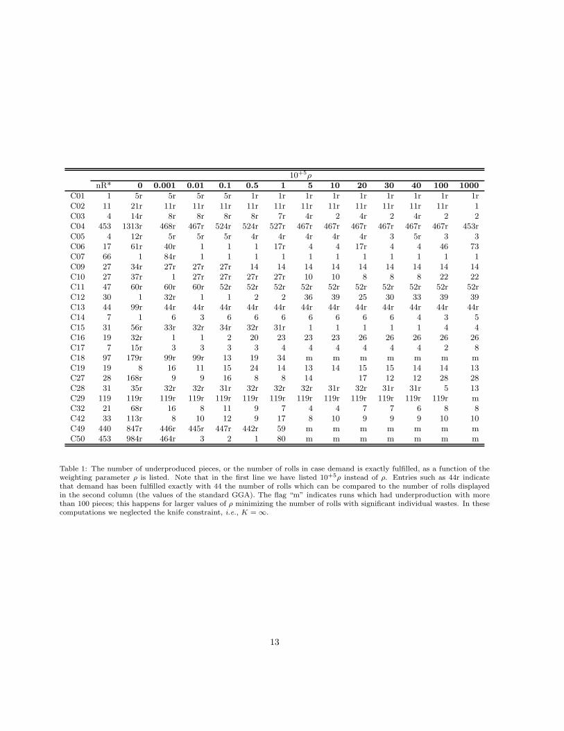
In the weighted objective function, the parame-ter ρ crucially effects the computed solution. Theresults in Table 1 reflect the delicate role of ρ. Forρ = 0, we obtain exact fulfillment of demand in al-most all cases. Deviation, as for case 7 with onepiece underfulfilled, can be explained by the differ-ence between the solution of the restricted masterproblem (0.371 in this case) to the MILP masterproblem (84 in this case). However, the price toreach exact demand fulfillment is high, which is re-flected in the large number of rolls. If we start withlarge values of ρ, minimizing the number of rollsis preferred and thus we are not surprised to seesubstantial underproduction. If we decrease ρ, atsome value, we exactly meet demand for the firsttime. Usually, the number of rolls needed to fulfilldemand exactly is identical to, or does not deviatetoo much from, the value obtained by the standardGGA. If we further decrease ρ, the number of rollsincreases in most cases.What is now the conclusion about the value of

ρ? For our problem instances, ρ = 0.000001 turnedout to be the best value, yielding good results in al-most all situations which occurred at our customer.However, this might be different in other situations.Thus, our advise is to experiment and analyze theresults.

3.6.3. CGA: Master Rolls with Different Widthsand Limited Availability

We modified the benchmark instances from Sec-tion 3.6.1 as follows: All data sets contain 3master rolls of different widths. The width ofthe master rolls were selected as follows: roll 2has width, B2, of the benchmark data set. Thewidth of roll 1 was reduced by about 30%, B1 =max{⌊0.7B2⌋,maxi Wi} allowing that the largestwidth can be produced, while the width of roll 3was set to B3 = ⌊1.2B2⌋.Table 2 summarizes the computational results for

K = ∞, i.e., the knife constraint has not been con-sidered, and for master rolls with different widths

and availability (equal to N for the three types);N1, N2 and N3 denote the number of rolls used. So-lutions computed with the exact demand constraintare indicated by an “E” in column “DS”. If no solu-tions existed with the exact demand constraint orif the relative gap was larger than 20%, we allowedoverproduction (“G” in column “DS”). However, inthis case, the relative waste (“%W”) does not countoverproduction as waste and is, thus, only of limiteduse.

Note that: (1) the CGA converges after a fewiterations (“IT”) leading to running times of a fewseconds. (2) Forcing exact demand satisfaction inthe master problem (MILP) for the patterns com-puted leads to relatively large GAPs. Allowingoverproduction results generally in smaller GAPs,but the modified round-up property does not hold(cf. Sect. 3.2). (3) The percentage waste (“%W”),when forcing exact demand satisfaction, is for mostinstances (except for “C01,” “C02,” “C03,” “C07,”“C49,” and “C50”) competitive and acceptable bypractitioners. The percentage waste for the cases ofoverproduction excludes the overproduced pieces.

The limits, Nr, on the number of available masterrolls requires us to think about the computation ofan initially feasible set, P0, of patterns. To generateP0, we solve the unlimited CSPs for each master rollwidth Br separately by the GGA. If P∗

r denotes theset of patterns in the optimal solution obtained forwidth Br, we obtain P0 as the union P0 := ∪rP

∗r .

If∑

r Nr is not too small, P0 allows us to computean initial feasible solution to the overall problem.Columns 3 to 5 in Table 2 shows that, in most cases,the larger master rolls are used up to their limits.

3.6.4. Exhaustion Method: Minimizing the Numberof Rolls and Patterns

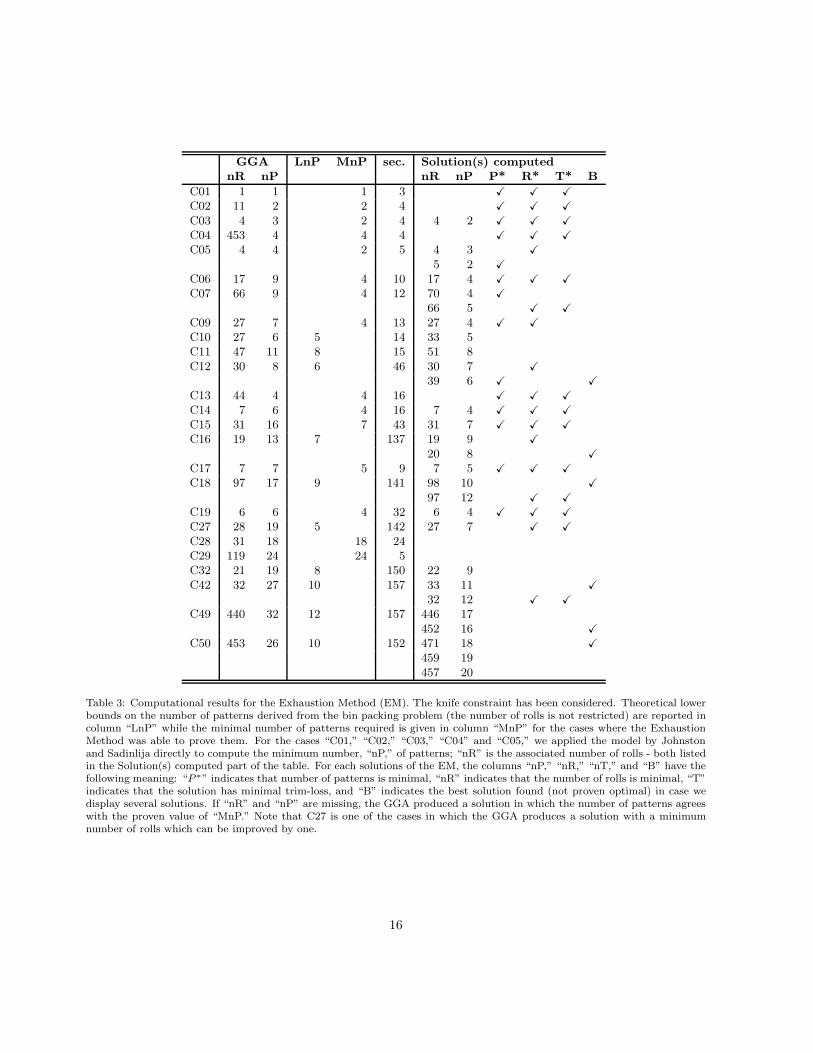
The Exhaustion Method is designed to overcomethe two main drawbacks of the GGA: The numberof patterns required tends to be too large and wehave overproduction. Table 3 summarizes the re-sults of the Exhaustion Method. We report on thesolution computed by the GGA; GGA provides anupper bound both on the minimal number of rollsand on the minimal number of patterns. Theoreti-cal lower bounds on the number of patterns derivedfrom the bin packing problem (the number of rolls isnot restricted) are reported in column “LnP” whilethe minimal number of patterns required is given incolumn “MnP” for the cases where the ExhaustionMethod was able to prove them.

12

10+5ρ

nR* 0 0.001 0.01 0.1 0.5 1 5 10 20 30 40 100 1000

C01 1 5r 5r 5r 5r 1r 1r 1r 1r 1r 1r 1r 1r 1rC02 11 21r 11r 11r 11r 11r 11r 11r 11r 11r 11r 11r 11r 1C03 4 14r 8r 8r 8r 8r 7r 4r 2 4r 2 4r 2 2C04 453 1313r 468r 467r 524r 524r 527r 467r 467r 467r 467r 467r 467r 453rC05 4 12r 5r 5r 5r 4r 4r 4r 4r 4r 3 5r 3 3C06 17 61r 40r 1 1 1 17r 4 4 17r 4 4 46 73C07 66 1 84r 1 1 1 1 1 1 1 1 1 1 1C09 27 34r 27r 27r 27r 14 14 14 14 14 14 14 14 14C10 27 37r 1 27r 27r 27r 27r 10 10 8 8 8 22 22C11 47 60r 60r 60r 52r 52r 52r 52r 52r 52r 52r 52r 52r 52rC12 30 1 32r 1 1 2 2 36 39 25 30 33 39 39C13 44 99r 44r 44r 44r 44r 44r 44r 44r 44r 44r 44r 44r 44rC14 7 1 6 3 6 6 6 6 6 6 6 4 3 5C15 31 56r 33r 32r 34r 32r 31r 1 1 1 1 1 4 4C16 19 32r 1 1 2 20 23 23 23 26 26 26 26 26C17 7 15r 3 3 3 3 4 4 4 4 4 4 2 8C18 97 179r 99r 99r 13 19 34 m m m m m m mC19 19 8 16 11 15 24 14 13 14 15 15 14 14 13C27 28 168r 9 9 16 8 8 14 17 12 12 28 28C28 31 35r 32r 32r 31r 32r 32r 32r 31r 32r 31r 31r 5 13C29 119 119r 119r 119r 119r 119r 119r 119r 119r 119r 119r 119r 119r mC32 21 68r 16 8 11 9 7 4 4 7 7 6 8 8C42 33 113r 8 10 12 9 17 8 10 9 9 9 10 10C49 440 847r 446r 445r 447r 442r 59 m m m m m m mC50 453 984r 464r 3 2 1 80 m m m m m m m

Table 1: The number of underproduced pieces, or the number of rolls in case demand is exactly fulfilled, as a function of theweighting parameter ρ is listed. Note that in the first line we have listed 10+5ρ instead of ρ. Entries such as 44r indicatethat demand has been fulfilled exactly with 44 the number of rolls which can be compared to the number of rolls displayedin the second column (the values of the standard GGA). The flag “m” indicates runs which had underproduction with morethan 100 pieces; this happens for larger values of ρ minimizing the number of rolls with significant individual wastes. In thesecomputations we neglected the knife constraint, i.e., K = ∞.

13

RC N N1 N2 N3 IT RMP IMP %G DS nR nP nR* nP* %W sec.

C01 1 0 1 0 1 405 405 0.00 E 1 1 1 1 7.92 0.26C02 4 3 4 4 1 8109 10466 22.51 E 11 5 11 2 18.97 0.54C03 2 2 2 0 3 714.8 910 21.45 E 4 4 4 3 10.80 0.49C04 165 90 164 165 2 2286.3 2289.0 0.11 E 419 6 453 4 2.30 0.82C05 2 1 1 2 3 87.95 783 87.95 E 4 4 4 4 3.69 0.77C06 7 7 7 4 1 355.5 569.0 37.52 E 18 9 17 9 1.16 0.32C07 24 19 24 24 1 3156.3 3260.0 3.18 E 67 10 66 9 10.62 0.28C09 11 4 11 11 2 4383 4383 0.00 E 26 8 27 7 3.17 0.51C10 11 5 10 11 5 2379.1 2953 19.43 E 26 9 27 6 1.77 1.68C11 17 10 16 17 3 9140.4 10686 14.46 E 43 18 47 11 5.70 0.74C12 11 10 8 11 3 4115.5 4318.0 4.69 E 29 12 30 8 3.37 2.71C13 18 11 16 17 4 220 460 52.17 E 44 22 44 4 0.23 11.39C15 12 7 12 11 2 150.6 267 43.58 E 30 17 31 16 0.33 4.67C16 7 6 5 7 7 479.3 2346 79.57 E 18 16 31 16 0.33 4.67C18 38 20 35 38 13 1094.9 1656 33.88 E 93 21 97 17 0.29 13.54C28 13 3 13 10 12 225 267 15.73 E 26 19 31 18 3.84 2.57C29 27 15 24 22 6 4656.5 4724 1.42 E 61 6 119 24 2.31 1.64C49 177 128 177 177 1 253360 254539 0.46 E 482 38 440 32 10.48 0.25C50 182 110 182 182 33 173297 174472 0.67 E 474 32 453 33 7.21 0.21

C02 4 3 4 4 2 8109 8467 4.22 G 11 4 11 2 15.34 0.31C03 2 2 1 2 2 688 732 6.01 G 5 4 4 3 6.08 0.53C05 2 1 2 2 3 75 88 14.77 G 5 4 4 4 0.25 0.79C06 7 7 7 7 3 174.2 195.0 10.67 G 21 6 17 9 0.17 0.84C13 18 8 17 18 5 220 224 1.78 G 43 14 44 4 0.00 1.84C14 3 2 3 3 4 44 50 12.00 G 8 8 7 6 0.00 1.32C15 12 7 12 12 4 109.5 115 4.76 G 31 17 31 16 0.00 1.09C16 7 7 7 7 16 177.9 266 33.12 G 21 11 19 13 0.30 1.74C17 3 1 3 3 17 27.2 31 12.41 G 7 7 7 7 0.00 5.50C18 38 31 38 38 11 512.4 518 1.08 G 107 14 97 17 0.29 13.54C19 5 4 4 1 5 67 111 39.64 G 9 9 6 6 0.02 1.37C27 12 12 12 6 3 212 233 9.01 G 30 24 28 19 0.01 8.66C32 8 8 8 8 7 117 135 13.33 G 24 20 21 19 0.01 7.71C42 21 20 13 5 44 165 188 12.23 G 35 29 33 11 0.01 14.33

Table 2: CSP with three different widths for the master rolls and limited roll availability. Solutions computed with the exactdemand constraint are indicated by an “E” in column “DS”. If no solutions existed with the exact demand constraint or if therelative gap was larger than 20%, we allowed overproduction (“G” in column “DS”). However, in this case, the relative waste(“%W”) does not count overproduction as waste and is, thus, only of limited use.

14

For the 25 real data instances tested, we observethat the Exhaustion Method finds a solution with(1) proven minimal number of rolls and proven min-imal number of patterns in 10 cases (“C01,” “C02,”“C03,” “C04,” “C06,” “C13,” “C14,” “C15,”“C17,” “C19”),(2) proven minimal number of rolls while reducingthe number of patterns used by at least 1 comparedto the GGA in 14 cases.The computational times never exceed 3 minutes,even for the largest instances with 50 orders.

4. 2D trim-loss Minimization

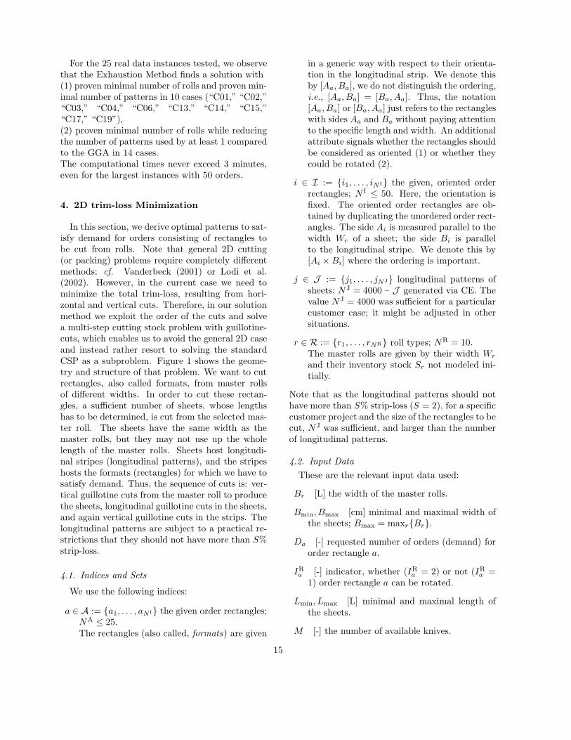
In this section, we derive optimal patterns to sat-isfy demand for orders consisting of rectangles tobe cut from rolls. Note that general 2D cutting(or packing) problems require completely differentmethods; cf. Vanderbeck (2001) or Lodi et al.(2002). However, in the current case we need tominimize the total trim-loss, resulting from hori-zontal and vertical cuts. Therefore, in our solutionmethod we exploit the order of the cuts and solvea multi-step cutting stock problem with guillotine-cuts, which enables us to avoid the general 2D caseand instead rather resort to solving the standardCSP as a subproblem. Figure 1 shows the geome-try and structure of that problem. We want to cutrectangles, also called formats, from master rollsof different widths. In order to cut these rectan-gles, a sufficient number of sheets, whose lengthshas to be determined, is cut from the selected mas-ter roll. The sheets have the same width as themaster rolls, but they may not use up the wholelength of the master rolls. Sheets host longitudi-nal stripes (longitudinal patterns), and the stripeshosts the formats (rectangles) for which we have tosatisfy demand. Thus, the sequence of cuts is: ver-tical guillotine cuts from the master roll to producethe sheets, longitudinal guillotine cuts in the sheets,and again vertical guillotine cuts in the strips. Thelongitudinal patterns are subject to a practical re-strictions that they should not have more than S%strip-loss.

4.1. Indices and Sets

We use the following indices:

a ∈ A := {a1, . . . , aN I} the given order rectangles;NA ≤ 25.The rectangles (also called, formats) are given

in a generic way with respect to their orienta-tion in the longitudinal strip. We denote thisby [Aa, Ba], we do not distinguish the ordering,i.e., [Aa, Ba] = [Ba, Aa]. Thus, the notation[Aa, Ba] or [Ba, Aa] just refers to the rectangleswith sides Aa and Ba without paying attentionto the specific length and width. An additionalattribute signals whether the rectangles shouldbe considered as oriented (1) or whether theycould be rotated (2).

i ∈ I := {i1, . . . , iN I} the given, oriented orderrectangles; N I ≤ 50. Here, the orientation isfixed. The oriented order rectangles are ob-tained by duplicating the unordered order rect-angles. The side Ai is measured parallel to thewidth Wr of a sheet; the side Bi is parallelto the longitudinal stripe. We denote this by[Ai ×Bi] where the ordering is important.

j ∈ J := {j1, . . . , jNJ} longitudinal patterns ofsheets; NJ = 4000 – J generated via CE. Thevalue NJ = 4000 was sufficient for a particularcustomer case; it might be adjusted in othersituations.

r ∈ R := {r1, . . . , rNR} roll types; NR = 10.The master rolls are given by their width Wr

and their inventory stock Sr not modeled ini-tially.

Note that as the longitudinal patterns should nothave more than S% strip-loss (S = 2), for a specificcustomer project and the size of the rectangles to becut, NJ was sufficient, and larger than the numberof longitudinal patterns.

4.2. Input Data

These are the relevant input data used:

Br [L] the width of the master rolls.

Bmin, Bmax [cm] minimal and maximal width ofthe sheets; Bmax = maxr{Br}.

Da [-] requested number of orders (demand) fororder rectangle a.

IRa [-] indicator, whether (IRa = 2) or not (IRa =1) order rectangle a can be rotated.

Lmin, Lmax [L] minimal and maximal length ofthe sheets.

M [-] the number of available knives.

15

GGA LnP MnP sec. Solution(s) computednR nP nR nP P* R* T* B

C01 1 1 1 3 X X X

C02 11 2 2 4 X X X

C03 4 3 2 4 4 2 X X X

C04 453 4 4 4 X X X

C05 4 4 2 5 4 3 X

5 2 X

C06 17 9 4 10 17 4 X X X

C07 66 9 4 12 70 4 X

66 5 X X

C09 27 7 4 13 27 4 X X

C10 27 6 5 14 33 5C11 47 11 8 15 51 8C12 30 8 6 46 30 7 X

39 6 X X

C13 44 4 4 16 X X X

C14 7 6 4 16 7 4 X X X

C15 31 16 7 43 31 7 X X X

C16 19 13 7 137 19 9 X

20 8 X

C17 7 7 5 9 7 5 X X X

C18 97 17 9 141 98 10 X

97 12 X X

C19 6 6 4 32 6 4 X X X

C27 28 19 5 142 27 7 X X

C28 31 18 18 24C29 119 24 24 5C32 21 19 8 150 22 9C42 32 27 10 157 33 11 X

32 12 X X

C49 440 32 12 157 446 17452 16 X

C50 453 26 10 152 471 18 X

459 19457 20

Table 3: Computational results for the Exhaustion Method (EM). The knife constraint has been considered. Theoretical lowerbounds on the number of patterns derived from the bin packing problem (the number of rolls is not restricted) are reported incolumn “LnP” while the minimal number of patterns required is given in column “MnP” for the cases where the ExhaustionMethod was able to prove them. For the cases “C01,” “C02,” “C03,” “C04” and “C05,” we applied the model by Johnstonand Sadinlija directly to compute the minimum number, “nP,” of patterns; “nR” is the associated number of rolls - both listedin the Solution(s) computed part of the table. For each solutions of the EM, the columns “nP,” “nR,” “nT,” and “B” have thefollowing meaning: “P ∗” indicates that number of patterns is minimal, “nR” indicates that the number of rolls is minimal, “T”indicates that the solution has minimal trim-loss, and “B” indicates the best solution found (not proven optimal) in case wedisplay several solutions. If “nR” and “nP” are missing, the GGA produced a solution in which the number of patterns agreeswith the proven value of “MnP.” Note that C27 is one of the cases in which the GGA produces a solution with a minimumnumber of rolls which can be improved by one.

16

strip-loss

vertical trim-loss

sheet 1 sheet 2

Figure 1: 2D paper cutting in three steps: 1st guillotine-cut (dotted line), 2nd longitudinal cuts, 3rd guillotine- cut (dashedvertical lines).

4.3. Variables

We use the following – mostly integer – variables:

µrj ∈ IN0 [−] states how often the sheet j canbe cut from roll r; only used in the masterproblem.

αrij ∈ IN0 [−] states how often the rectangle[Ai ×Bi] is contained in the sheet j of roll r.This variable is used in the subproblem and isthe only independent variable of the subprob-lem and can be obtained explicitly.

ℓrj ∈ IN0 [mm] specifies the length of the sheetj of roll r; ℓrj depends on all αrij .

wp ≥ 0 [−] states the trim-loss of pattern p; 0 ≤wp ≤ B.

4.4. Overview of the Algorithmic Components

The algorithm is structured as follows:

1. The order rectangles [Aa, Ba], given throughtheir length and width, are duplicated andyield the oriented rectangles [Ai × Bi]. Theindices i and a are connected as follows

a(i) :=

{

i , 1 ≤ i ≤ NA

i−NA , NA + 1 ≤ i ≤ 2NA

which yields

[Ai ×Bi] :={

[Aa(i) ×Ba(i)] , 1 ≤ i ≤ NA

[Ba(i) ×Aa(i)] , NA + 1 ≤ i ≤ 2NA .

or (∀{i | 1 ≤ i ≤ NA})

[Bi′ ×Ai′ ] = [Ai ×Bi] , i′ := i+NA .

The demand for order rectangle [Aa, Ba] canthus be fulfilled the by orientated rectangles iand i′.

2. For each master roll r with width Wr, enumer-ation is used to

(a) generate up to NJ stripe partitions (lon-gitudinal patterns) which are compatibleto {Ai} (the width of the stripes corre-spond to the width Ai) – thus, the strip-loss and the width of each longitudinalstrip are known – and

(b) solve the corresponding subproblem (min-imization of the vertical trim-loss of astripe partition, see Section 4.5.2) – thus,the vertical trim-loss and the total trim-loss of each roll as well as its length ℓrj areknown. In addition, the solution of thesubproblem gives us the number, N tot

raj, oforder rectangles [Aa, Ba] covered by sheetrj.

3. The master problem is a partitioning prob-lem. This MILP problem calculates how manysheets of length ℓrj are required in order tomeet the demand for order rectangles [Aa, Ba].

4.5. Master- and Subproblem

4.5.1. The Master Problem: Partitioning Model

The master problem minimizes the total trim-loss, i.e., the model makes use of the following ob-jective function

min∑

r∈R

∑

j∈J

Wrjµrj , (29)

with trim-lossWrj for the sheet rj; the integer vari-able µrj denotes its multiplicity. The demand equa-

17

tion reads

Da ≤∑

r∈R

∑

j∈J

N totrajµrj ≤ Da +Dover

a , ∀a (30)

or

Di ≤∑

r∈R

∑

j∈J

N totrijµrj +

∑

r∈R

∑

j∈J

N totr,i+NA,jµrj

≤ Di +Doveri , ∀{i | 1 ≤ i ≤ NA} . (31)

The multiplicity variables can be bounded by

µrj ≤ maxa

{⌈

Da +Dovera

max{1, N totraj}

⌉}

, ∀{rj} .

(32)The integrality constraints are given by

µrj ∈ IN0 , ∀{rj} . (33)

For operative reasons, it might be useful to use onlyrolls of a particular width r∗, because several of suchrolls might be cut on top of each other simultane-ously (e.g., up to four rolls can be cut at the sametime in our case). In this case, model (29)-(33)is substituted by a sequence of NR models, whereeach time only one of the NR roll widths is used; theuser can then select the appropriate solution. Carehas to be taken when restricting overproduction;this can lead to infeasibilities when considering asingle roll width. It might be useful to consider agoal programming approach which first minimizesthe overproduction and second the trim-loss, or viceversa.Alternatively, we introduce the binary variables

δr which is 1 if a roll of width r is used and 0 oth-erwise. The following equation

∑

r∈R

δr = 1

and inequalities

µrj ≤ δr , ∀{rj}

need to be added to the model.The inventory stock can be modeled with the fol-

lowing approach: Each individual master roll t byits roll type r (width) and its (remaining) lengthLt. Then, the following constraints

µrj =∑

t | Rt=ord(r)

µrjt , ∀{rj}

and∑

t | Rt=ord(r)

Lrjµrjt ≤ Lt , ∀{rjt}

need to be satisfied. The integer variable µrjt de-scribes, how many sheets of type rj are to be cutfrom master roll t.

4.5.2. The Subproblem

For a given distribution of longitudinal cuts for asheet rj – i.e., a system of values Ai, 1 ≤ i ≤ 2NA

– the task is to decide on the lengths ℓrj of the sheetsuch that the vertical trim-loss wver

rj , the total trim-

loss wtotrj , or the wrel

rj striploss is minimized. Theinteger variable αrij defines the amount of timesthe oriented rectangle [Ai ×Bi] is contained in thelongitudinal stripe i (defined through Ai) with mul-tiplicity Npat

rij . This enables us to express the verti-cal trim-loss as

wverrj :=

∑

i | Npatrij

>0

(

Npatrij Ai

)

srij ,

srij := ℓrj −Biαrij .

The absolute and relative trim-loss – the latter lead-ing to a MINLP problem – are given through

wtotrj := Wrℓrj + wver

rj

andwrel

rj := Wr + wverrj /ℓrj .

The relative trim-loss measure for the objectivefunction leads to more large sheets close to the limitLmax. However, they will contain more formats.The model is restricted by

Lmin ≤ ℓrj ≤ Lmax

and (∀{rij | Npatrij = 0})

αrij = 0 ,

αminrij :=

⌈

Lmin

Bi

⌉

≤ αrij ≤

⌊

Lmax

Bi

⌋

=: αmaxrij .

4.5.3. Explicit Solution of the Subproblems

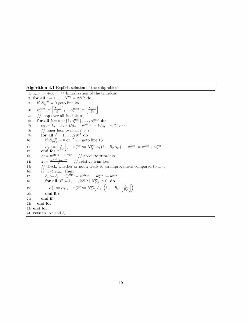
For computational efficiency, we suggest to calcu-late the solution of the subproblems and all deriveddata (αrij , ℓrj) simultaneously with CE. The struc-ture of the subproblem allows us to compute theoptimal values of αrij analytically. The flowchartfor the explicit calculation of αrij for sheet rj issummarized in Algorithm 4.1.Note that this explicit solution method works forthe absolute as well as the relative trim-loss.

18

Algorithm 4.1 Explicit solution of the subproblem

1: zmin := +∞ // Initialization of the trim-loss2: for all i = 1, . . . , NW = 2NA do3: if Npat

ij = 0 goto line 26

4: αmini :=

⌈

Lmin

Bi

⌉

, αmaxi :=

⌊

Lmax

Bi

⌋

5: // loop over all feasible αi

6: for all k = max{1, αmini }, . . . , αmax

i do7: αi := k, ℓ := Bik, wstrip := Wℓ, wver := 08: // inner loop over all i′ 6= i9: for all i′ = 1, . . . , 2NA do

10: if Npatri′j = 0 or i′ = i goto line 15

11: αi′ :=⌊

ℓBi′

⌋

, wveri′ := Npat

ij Ai (ℓ−Bi′αi′), wver := wver + wveri′

12: end for13: z := wstrip + wver // absolute trim-loss

14: z := wstrip+wver

ℓ// relative trim-loss

15: // check, whether or not z leads to an improvement compared to zmin

16: if z < zmin then17: ℓ∗ := ℓ, wstrip

∗ := wstrip, wver∗ := wver

18: for all i” = 1, . . . , 2NA | Npati”j > 0 do

19: α∗i” := αi”, wver

i” := Npatri”jAi”

(

ℓ∗ −Bi”

⌊

ℓ∗Bi”

⌋)

20: end for21: end if22: end for23: end for24: return α∗ and ℓ∗

19

4.5.4. Assignment of Sheets to the Orders

If rolls and sheets are treated as individuals, aresult such as

Order A25022007 is satisfied by:

Sheet 1-433 of roll R102-stock0017

Sheet 22-40 of roll R152-stock0002

enables us to know how the orders are satisfied.Further, we might be interested what happens witheach rectangle cut from a roll and sheet, i.e., forwhich order it is intended.The assignment of rectangles in the sheets to the

original orders is done after optimizing the trim-loss. The algorithm does not require any additionaldata or results other than the ones provided forthe trim-loss minimization problems. However, thefollowing derived data are necessary:

i = i(a) [-] rectangle i, corresponding to order a[derived entry date].

i′ = i′(a) [-] rectangle i′, obtained through rota-tion of rectangle i and corresponding to ordera [derived entry date].

Da [-] the order quantity for order a [derived en-try date].

Nrji [-] the quantity how often rectangle i is con-tained in sheet rj.

Nrji′ [-] the quantity, how often rectangle i as-sociated with rectangle i′ is contained in sheetrj.

µrj [-] the quantity, how often sheet rj is used.

Xrja := µrj (Nrji +Nrji′) [-] the quantity, howoften the order a corresponding to rectangles iand i′ are produced by sheet rj.

The model and algorithm requires the followingvariables:

xarj ∈ IN [−] the number of rectangles, cut fromthe sheet rj, used for order a.The variables can assume values between 0 andXrj (Nrji +Nrji′ ).

yarj ∈ {0, 1} [−] indicates, whether (1) or not(0) order a is served by sheet rj.

The goal is to minimize the sum over all quantitiessa :=

∑

rj yarj, which measures how many sheetsserve order a, i.e.,

min∑

a∈A

sa =∑

a∈A

∑

rj

yarj .

The demand satisfaction is a constraint

min∑

rj

xarj = Da .

The variables xarj are restricted by

xarj ≤ min{Xarj, Da}yarj ; ∀{arj} .

Note: This assignment problem is solved after theminimization problem. The quality of the resultswith respect to trim-loss and the quantity of sheetsis not affected.

4.6. Computational Results

We use the same computational framework as forthe 1D case (cf. Sect. 3.6). The details of the12 test instances used are summarized in Table 4.Each 2D instance is characterized by the numberof orders, NA, and the size of the rectangles to becut (i.e., length and width), quantity of requestedpieces, number of different-size master rolls, NR,and their widths. Each master roll is assumed tohave infinite length.

The results for the 2D test instances are summa-rized in Table 5. For the reported optimal solu-tion, NS is the number of different sheets required,“S” (surplus) indicates the number of overproducedpieces, “%W” is the relative waste in percent and“T” shows the time in milliseconds. The interpre-tation of the “Optimal Solution” is illustrated bythe example 1,213×[4A2·3+A1r·5]→2: The “→2”indicates that this sheet is cut from roll type 2 withmultiplicity 1,213. “4A2·3” expresses that order A2enters Npat

rij = 3 times and that αrij = 4; the to-tal contribution of that sheet to order A2 is thus1, 213 · 4 · 3 = 14, 556 pieces. The term “A1r·5”indicates that the sheet contains order A1 in ro-tated placement and contributes 1, 213·1·5 = 6, 065pieces.

The table shows that the model and algorithmcan handle various different situations regardingsize of the rectangles and from small demand num-bers to large ones reaching up to 1,000,000. All re-sults were obtained in fractions of one second. Froma practical point, sheets which are used only once orwith small multiplicity, are not desirable. As theydo not contribute many pieces, they are usually ne-glected – little underproduction is not a problem.

20

Orders Master Roll

NA Dimensions [mm] Quantity NR Width [mm]

2D01 2 21×22, 25×27 20,812 21,367 3 102 122 1522D02 3 36×80, 26×85, 24×33 8,000 8,000 20,000 2 102 1522D03 9 24×36, 36×80, 29×100 20,000 15,000 5,000 3 152 122 102

39×103, 29×100, 39×93 5,000 5,000 5,00019×75, 29×68, 19×29 5,000 15,000 15,000

2D04 1 101×43.5 10,500 1 1272D05 3 48×110, 43.5×101, 37.5×87 15,000 15,000 20,000 1 1222D06 1 3×2 “Schnipselfall” 1,000,000 1 1022D07 6 43.5×101, 33.5×79, 28×68 10,500 70,500 43,000 2 127 122

23×58, 48×110, 53×122 21,500 2,000 4,5002D08 1 3×2 “Schnipselfall” 1,000,000 1 1022D09 2 as 1 but 85% striploss, 100 pc overproduction 3 102 122 1522D10 6 as 7 but 82% striploss as 7 2 127 1222D11 1 as C08 10 pc overproduction 1 1022D12 1 50×50 5556 8 102 112 122 152

162 182 203 228

Table 4: Data for the 2D test instances.

NS Optimal Solution S %W T

2D01 6 1×[3A2·2+A2r·2]→1 , 2×[4A2·4+A1r·5]→2 0 0.65 78290×[6A1·5+A1·4]→3 , 1×[6A2·2]→31×[3A1·6+3A1·5]→3 , 1,007×[4A2·6+A1r·5]→3

2D02 5 1×[3A2·1+A3·2]→1 , 1,996×[3A2·2]→1 , 1×[2A2·1+3A3·4]→2 0 3.87 1092,665×[2A1·1+3A2·2]→2 , 1,335×[1A1r·1+2A3r·3]→2

2D03 9 625×[8A7·1]→1 , 1,000×[A2·1+2A2r·1]→1 0 1.84 1252,750×[2A2r·4+A8r·5]→1 , 1,000×[A9·5+A1·6+A3·5]→11,000×[A9·5+A1·6+A5·5]→1 , 50×[A1·2]→2 , 2,500×[A1·3+A4·1]→32,500×[A6r·1+A9r·2]→2 , 1,250×[A8·1+A9r·2]→2

2D04 1 10,500×[A1r·1]→1 0 20.47 472D05 3 10,000×[1A2·1+2A3·1]→1 , 5,000×[A2r·1]→1 , 15,000×[A1r·1]→1 0 11.47 472D06 1 258×[102A1·38]→1 8 0 502D07 8 1×[2A2·1+2A3·1]→1 , 8,350×[3A2·1+A3·1]→1 , 0 4.30 47

1,852×[2A2·2+A4r·7]→1 , 4,777×[2A3·2+A3r·5]→1 ,1×[2A3r·5+A4r·6]→1 , 10,500×[A1·1+A2r·3]→1 ,2,000×[A5·1+A2r·3]→1 , 4,500×[A6·1]→2

2D08 1 1,548×[34A1·19]→1 8 0 472D09 2 1,213×[4A2·4+A1r·5]→2 , 492×[6A1·5+A2·4]→3 3 9 0.66 622D10 8 6,382×[2A2·1+2A3·1]→1 , 17,494×[3A2·1+A4·1]→1 , 0 8.08 62

2,000×[A4·2+A5·1+A6·1]→1 , 7,559×[4A3·1]→2 ,5,250×[2A1·5+A2·6]→2 , 1×[3A4·1+A6·3]→2 ,1×[2A2·1+A6·3]→2 , 1,249×[2A6·1]→2

2D11 1 as C08 8 0 472D12 1 1,852×[3A1·1]→4 0 1.32 312

Table 5: Optimal solutions computed by the polylithic solution method for the test instances of Table 4.

21

5. Current-Edge Cutting Stock Problems

We assemble various CSPs which are at the fore-front of research or cannot be found in the litera-ture.

5.1. CSPs Under Uncertainty

An important practical challenge is how to dealwith variations in demand. We follow the spirit byBeraldi et al. (2009) and treat the demand stochas-tically: In the first stage, decisions on the choice ofpatterns have to be made to satisfy first stage de-mand (Di) while their multiplicity can be adjustedin a second-stage when the stochastic second-stagedemand (Dis) unfolds. The task is then to minimizethe total expected number of patterns used.The column enumeration procedure (cf. Sect.

3.3) can be adjusted in a straight forward manner todeal with demand uncertainty. Once the columns(collected in set P ′) have been enumerated, we solvethe following MILP:

min∑

p∈P′

(

µp +∑

s∈S

psµps

)

,

with probability ps of scenario s occurring, subjectto the first-stage demand-fulfill inequalities (8), thesecond-stage demand constraints

∑

p∈P′

Nipµps ≥ Dis , ∀{is} ,

and the connection of the first-stage and second-stage pattern

δp ≤ µp ≤ Mpδp , ∀p ∈ P ′

and

µps ≤ Mpδp , ∀p ∈ P ′ , ∀s ,

where binary variable δp indicates whether or notpatter p is used in the first stage or not and Mp isa sufficiently large constant. We require integralityon the decision variables

µps ∈ IN0 , ∀p ∈ P ′ , ∀s

and

δp ∈ {0, 1} , ∀p ∈ P ′ ,

as well as integrality constraint (9).Alem et al. (2010) also consider stochastic de-

mand for CSPs. However, the first stage deci-sion is on the multiplicity and pattern choice where

the recourse decisions determine over- or under-production of the stochastic demand realized. Theobjective is then to minimize the cutting cost pluspenalty cost for over- and under-production. Theresulting problem structure allows us to apply a col-umn generation approach.

5.2. CSPs with Tolerances

In the literature, cutting stock problems appearwith certain number of order rolls demanded. How-ever, in reality, the orders are often specified inweight. If one has master rolls of different lengths(!) available, the total weight ordered is subject todifferent number of rolls cut to a certain pattern.Both, the ordered weights and widths, are subjectto tolerances.

5.3. CSPs with Limited Inventory

In Section 3.5.5 we have provided a CGA for thesimplest case of master rolls with different widthsand limited stock availability, but under the as-sumption that all have the same length (usually, in-finity). However, on stock may imply, that the rollson stock have also finite and different lengths. Thiscase may occur under certain production philoso-phies and forces us to treat rolls as individuals.

5.4. CSPs and Simultaneous Production Planningand/or Scheduling

These problems are really hard as we have to de-liver at certain due dates but there are already ex-amples in the literature as outlined in Section 2.Here we find make-to-stock versus make-to-order(and mixed strategies). This class of problems ischallenging as cutting procedures and productionscheduling vary from case to case.

6. Paper Industry and Optimization

In recent times, the paper industry has vigorouslycut back their capacity, rising the prices. Rising en-ergy and raw material costs pressure the manufac-turers. Many machines were shut down worldwide.Also, the concentration process has continued.

6.1. Optimization Software: Importance and Fi-nancial Impact

The use of automated, software-based waste opti-mization provides great benefits to all producers ofrolls or formats such as paper mills, film producersand steelmakers.

22

A manually performed cut plan by a productionplanner, even though s/he might have significantexperience and knowledge, is, depending on thecomplexity, very time consuming and reaches, asopposed to a software-based plan, usually not theoptimum. This becomes even more significant forproducers with very different widths or format sizesand different machines.Our customers use the trim optimization both

when determining the optimal width of the par-ent rolls and when planning secondary productionprocesses. Waste optimization, integrated into theplanning process, is an essential, indispensable ele-ment of the short- and long-term production plan-ning. Depending on the complexity of the process,using the integrated waste optimization, even anautomated production planning is possible, e.g., aweekly schedule.For paper factories, which produce only standard

or simple cutting patterns, mathematical optimiza-tion may not be beneficial. Manual results are hardto beat for plants with very standardized productportfolio. In contrast, for plants which encounter abroad spectrum of products, our experience is a fol-lows. Depending on the complexity of their produc-tion structure, our customers confirmed 3-6 % re-duced trim-loss, comparing mathematical optimiza-tion based cutting stock solutions to their manualprocedures.Let us inspect this in detail for a typical customer

producing special paper: For an annual productionof 50,000 tons a trim-loss reduction of 3% saves1,500 tons per year. Even if the trim loss is usedin a recycling mill as raw material, the total sav-ing is 285,000 Euro production costs at the papermachine if we apply typical production cost of 190Euro per ton of produced paper, not consideringthe raw material price. Those paper factories whichcannot recycle the savings are significantly higher.The one-time purchase cost for our computer-basedsolution is about 30,000 to 40,000 Euro. Under theconditions of this example, the Return of Invest-ment (ROI) is reached after only two months. Afurther advantage is the decrease of dependence onemployees with many years of knowledge and expe-rience in the creation of manual cutting plans.On a global scale, the financial benefit of opti-

mization tools in the cutting paper industry varies,e.g., dependent on the machine type and order va-riety. In our experience, manual plans exhibit anaverage waste of between 3-5%, while optimizationyields in less than 2% waste, often below 1%. One

percentage waste minimization may lead to an an-nual saving of one million Euro per paper machine.

6.2. Outlook

In our experience, the diversification of ourclients’ products and the industry as a whole in-creases steadily, so that the use of a software-supported, automated production planning with in-tegrated cutting stock optimization becomes moreand more a necessity. Solving cutting stock prob-lems is not an isolated activity any longer.

7. Conclusions

Motivated by challenges arising in the paper in-dustry, we have presented various polylithic solu-tion approaches to model and solve a testbed of 1Dand 2D real-world cutting problems. The meth-ods are implemented in GSE’s ERP system. Wehave developed new column generation approachesto treat problems with different master roll widths,limited number of master rolls on stock, or prob-lems in which underproduction is allowed but tobe minimized. Numerical experiments demonstratethe value of these approaches and in some data in-stances also suggest either the use of Branch&Pricetechniques or other solution methods like the Ex-haustion Method, which is very efficient and pro-duces near optimal solutions for minimizing thenumber of patterns. The presented polylithic so-lution methods yield practically superior solutionscompared to the standard GGA, with practicallyfeasible computational times.As each paper producing company has its own

production processes specific cutting machines, themapping of reality and abstraction into a mathe-matical model and algorithm has, to our experience,the highest priority to receive the appreciation ofour clients. Besides this, future research and ef-ficient mathematical techniques on the integrationof CSPs into the production planning process andthe incorporation of uncertainty would be very wel-come.

Appendix A. Post-Processing of OptimalGGA/CGA Solutions

The GGA/CGA produces solutions which areminimal in the number of rolls but are occasion-ally lead to overproduction exceeding the demand

23

Di by Si pieces. We have developed three heuris-tics to eliminate overproduction: The first one justmodifies patterns, the second one modifies patternsand generates new ones, and the third one is a com-bination of both.In Case 1, for a given Si, we can find a pattern p

used with multiplicity Mp and Nip > 0 subject to

∃κ | Si = κMp ∧ κ = 1, 2, . . . , Nip ∈ IN ,(A.1)

where κ is an integer number. In this simple case,we modify pattern p as follows:

Nip := Nip − κ and wp := wp + κWi .

This implies that the number of pieces i, producedby using pattern p Mp times, is reduced by Si =κMp.Case 2 is more complicated. Let Rip := NipMp

denote the number of pieces i produced by usingpattern p Mp times. If we allow a new pattern p′,in which item i occurs µ times, to be used π times,the reduction condition reads now

(Nip − κ) (Mp − π) + µπ = Rip − Si

or(κ+ µ−Nip)π = κMp − Si , (A.2)

where π reduces the number of rolls cut to patternp. The term µπ considers the number of pieces oftype i produced by using the new pattern π times.Depending on the solution of (A.2), p′ does not con-tain item i at all (Np′i = 0) or has a reduced numberof it (Np′i < Nip) while others items i′ remain un-changed (Ni′p′ = Nip). For π = 0 we obtain thesimple case (A.1) above; it suffices to modify justone pattern.We solve the diophantine equation (A.2) by tests

in three nested loops:

π = 0, 1, . . . ,

k = 1, 2, . . . , Npi ,

µ = 0, 1, . . . .

The existing pattern p is modified by

Nip → Nip − κ and Mp → Mp − π .

For p′, item i and all other items i′ 6= i we apply

Ni′p′ → Nip ,

Nip′ → µ ,

Mp′ → π .

Unfortunately, there are still situations not cov-ered by Case 1 and Case 2. Let us illustrate thisfor item i = 14 (also called A14) by the followingexample with D14 = 1:

item Nip Mp

p11 A14 1 2p12 A14 1 5p23 A14 1 1

We have S14 = 7 surplus items. The patterns p11,p12 and p23 contain other items not relevant here.The equality (A.1) Si = κMp does not have a so-lution for κ ≤ 1; similarly, (A.2) does not have asolution. The best we could do is to eliminate A14in p23 which leaves a surplus of S′

14 = 6.Therefore, we add Case 3. For those widths i

with Si > 0 we generate a list Li := {p′1, p′2, p

′3, . . .},

which contains those patterns in which item i oc-curs, i.e., for all elements p′m ∈ Li we have: Nipm

>0 with pm = p(p′m) for all m. Now we check for allm, whether κ ≥ 1 exists with κMp ≤ Si. If it ex-ists, item i in pattern pm is eliminated k times andwe obtain S′

i := Si − κMp. If S′i > 0, we continue

the test for the next m and pattern pm until allpatterns in Li have been tested. If after this, westill have S′

i > 0, we continue with Case 2.

Appendix B. Deriving the Pricing Problem

In this section, we briefly describe how the pricingproblems of the cutting stock problem are derived.Let the master problem (minimization problem)

contain all possible patterns P ; the restricted mas-ter problem the patterns P ′ ⊆ P . An optimal so-lution of restricted master problem defines also anoptimal solution for the master problem, if all thereduced cost

cp − πAp ≥ 0 ∀p ∈ P (B.1)

with objective function coefficient cp for variableµp, (vector of) dual variables π of all functionalconstraints and Ap being the constraint coefficientmatrix of variable µp.Thus the pricing problem is obtained my mini-

mizing (B.1) over all p. Naturally, the constraintsof the pricing problem ensure that the newly com-puted pattern is feasible, i.e., is part of the set P .Let us illustrate this by the objective function

term

∑

r∈R

∑

p∈P′

r

(

Br −∑

i∈I

(

Wi − 1)

Nip

)

µp (B.2)

24

occurring in (27). From this term and the inequal-ities (28)

∑

p∈P′

r

µp ≤ Nr , ∀r , (B.3)

and (8)∑

p∈P′

Nipµp ≥ Di , ∀i , (B.4)

we had derived the pricing problem

z∗r := min

(

Br −∑

i∈I

(

Wi − 1)

αi − πr −∑

i∈I

πiαi

)

.

(B.5)We note in (B.5) that the

∑

p∈P′

rhas disappeared,

and that all occurrences of Nip have been replacedby αi. Instead of

∑

r∈R we have to deal with rindependent pricing problems to be solved. Thecoefficients appearing with the Lagrange multipliersπr and πi are those in (28) and (8) appearing withthe µp variables.

References

Alem, Jr., D., Munari, Jr., P., Arenales, M., Ferreira, P.,2010. On the cutting stock problem under stochastic de-mand. Annals of Operations Research 179, 169–186.

Alves, C., de Carvalho, J. M. V., 2007. Accelerating columngeneration for variable sized bin-packing problems. Euro-pean Journal of Operational Research 183 (3), 1333–1352.

Alves, C., Macedo, R., de Carvalho, J., 2009. New LowerBounds Based on Column Generation and Constraint Pro-gramming for the Pattern Minimization Problem. Com-puters & Operations Research 36, 2944–2954.

Amor, Hatem Ben de Carvalho, J. M. V., 2005. CuttingStock Problems. In: Desrosiers, G. D. J., Solomon, M. M.(Eds.), Column Generation. Springer, New York, pp. 131–161.

Arbib, C., Marinelli, F., 2005. Integrating process optimiza-tion and inventory planning in cutting-stock with skivingoption: An optimization model and its application. Euro-pean Journal of Operational Research 163 (3), 617–630.

Belov, G., Scheithauer, G., 2006. A Branch-and-Cut-and-Price Algorithm for One-Dimensional Stock Cutting andTwo-Dimensional Two-Stage Cutting. European Journalof Operational Research 171, 85–106.

Beraldi, P., Bruni, M., Conforti, D., 2009. The stochastictrim-loss problem. European Journal of Operational Re-search 197, 42–49.

Cui, Y., Zhao, Z., 2013. Heuristic for the rectangular two-dimensional single stock size cutting stock problem withtwo-stagged patterns. European Journal of OperationalResearch 231, 288–298.

Dyckhoff, H., Jan. 1990. A Typology of Cutting and Pack-ing Problems. European Journal of Operational Research44 (2), 145–159.

Gilmore, P., Gomory, R., 1961. A Linear Programming Ap-proach to the Cutting Stock Problem. Operations Re-search 9, 849–859.

Gramani, M. C. N., Franca, P. M., 2006. The combined cut-ting stock and lot-sizing problem in industrial processes.European Journal of Operational Research 174 (1), 509–521.

Gramani, M. C. N., Franca, P. M., Arenales, M. N., 2009. ALagrangian Relaxation Approach to a Coupled Lot-sizingand Cutting Stock Problem. International Journal of Pro-duction Economics 119, 219–227.

Haessler, R. W., 1971. A Heuristic Programming Solution toa Nonlinear Cutting Stock Problem. Management Science17, B793–B802.

Haessler, R. W., 1992. One-dimensional cutting stock prob-lems and solution procedures. Math. Comput. Model.16 (1), 1–8.

Haessler, R. W., Sweeney, P. E., 1991. Cutting Stock Prob-lems and Solution Procedures. European Journal of Op-erational Research 54, 141–150.

Haessler, R. W., Talbot, F. B., 1983. A 0-1 Model for Solvingthe Corrugator Trim Problem. Management Science 29,200–209.

Harjunkoski, I., Westerlund, T., Porn, R., Skrifvars, H.,1998. Different transformations for solving non-convex byMINLP. European Journal of Operational Research 105,594–603.

Holthaus, O., 2002. Decomposition approaches for solvingthe integer one-dimensional cutting stock problem withdifferent types of standard lengths. European Journal ofOperational Research 141 (2), 295–312.

Johnston, R., Sadinlija, E., 2004. A New Model for CompleteSolutions to One-Dimensional Cutting Stock Problems.European Journal of Operational Research 153, 176–183.

Kallrath, J., 2009a. Combined Strategic Design and Oper-ative Planning in the Process Industry. Computers andChemical Engineering 33, 1983–1993.

Kallrath, J., 2009b. Cutting Circles and Polygons from Area-Minimizing Rectangles. Journal of Global Optimization43, 299–328.

Kallrath, J., 2011. Polylithic Modeling and Solution Ap-proaches Using Algebraic Modeling Systems. Optimiza-tion Letters 5, 453–466.

Kallrath, J., Rebennack, S., 2014. Cutting Ellipses fromArea-Minimizing Rectangles. Journal of Global Optimiza-tion, to appear.

Li, S., 1996. Multi-Job Cutting Stock Problem with DueDates and Release Dates. The Journal of the OperationalResearch Society 47 (4), 490–510.

Lodi, A., Martello, S., Monaci, M., 2002. Two-dimensionalpacking problems: A survey. European Journal of Opera-tional Research 141 (2), 241–252.

McDiarmid, C., 1999. Pattern Minimisation in Cutting StockProblems. Discrete Applied Mathematics 98, 121–130.

Poldi, K. C., Arenales, M. N., 2009. Heuristics for the one-dimensional cutting stock problem with limited multiplestock lengths. Computers & OR 36 (6), 2074–2081.

Poltroniere, S. C., Poldi, K. C., Toledo, F. M. B., Arenales,M. N., 2008. A coupling cutting stock-lot sizing problemin the paper industry. Annals OR, 91–104.

Porn, R., Harjunkoski, I., Westerlund, T., 1999. Convexifica-tion of different classes of non-convex MINLP problems.Computers & Chemical Engineering 23, 439–448.

Rebennack, S., Kallrath, J., Pardalos, P. M., 2009. ColumnEnumeration based Decomposition Techniques for a Classof Non-convex MINLP Problems. Journal of Global Op-timization 43, 277–297.

Reinertsen, H., Vossen, T. W. M., 2010. The one-dimensional

25

Cutting Stock Problem with Due Dates. European Jour-nal of Operational Research, 701–711.

Rodrıguez, M. A., Vecchietti, A., 2008. Enterprise optimiza-tion for solving an assignment and trim-loss non-convexproblem. Computers and Chemical Engineering 32, 2812–2822.

Santos, M. O., Almada-Lobo, B., Aug. 2012. Integrated pulpand paper mill planning and scheduling. Comput. Ind.Eng. 63 (1), 1–12.

Scheithauer, G., Terno, J., 1995. The modified integer round-up property of the one-dimensional cutting stock problem.European Journal of Operational Research 84, 562–571.

Trkman, P., Erjavec, J., Gradisar, M., 2009. Cutting as aContinuous Business Process. Economic and Business Re-view 11 (4), 285–300.

Trkman, P., Gradisar, M., 2007. One-dimensional cuttingstock optimization in consecutive time periods. EuropeanJournal of Operational Research 179 (2), 291–301.

Vanderbeck, F., 2000. Exact Algorithm for Minimising theNumber of Setups in the One-dimensional Cutting StockProblem. Operations Research 48, 915–926.

Vanderbeck, F., 2001. A nested decomposition approach to athree-stage, two-dimensional cutting-stock problem. Man-agement Science 47 (6), 864–879.

Wascher, G., Haußner, H., Schumann, H., Dec. 2007. An im-proved typology of cutting and packing problems. Euro-pean Journal of Operational Research 183 (3), 1109–1130.

Yanasse, H. H., Pinto Lamosa, M. J., 2007. An integratedcutting stock and sequencing problem. European Journalof Operational Research 183 (3), 1353–1370.

26