some aspects of analytic number theory: parity ... · some aspects of analytic number theory:...
TRANSCRIPT
SOME ASPECTS OF ANALYTIC NUMBER THEORY:
PARITY, TRANSCENDENCE, AND MULTIPLICATIVE
FUNCTIONS
by
Michael J. Coons
B.A., The University of Montana, 2003
M.S., Baylor University, 2005
a thesis submitted in partial fulfillment
of the requirements for the degree of
Doctor of Philosophy
in the Department
of
Mathematics
c© Michael J. Coons 2009
SIMON FRASER UNIVERSITY
Spring 2009
All rights reserved. This work may not be
reproduced in whole or in part, by photocopy
or other means, without the permission of the author.

APPROVAL
Name: Michael J. Coons
Degree: Doctor of Philosophy
Title of thesis: Some aspects of analytic number theory: parity, transcen-
dence, and multiplicative functions
Examining Committee: Dr. Steven Ruuth
Chair
Dr. Peter B. Borwein
Senior Supervisor, Simon Fraser University
Dr. Stephen K. K. Choi
Co–Supervisor, Simon Fraser University
Dr. Nils Bruin
Supervisory Committee, Simon Fraser University
Dr. Karen Yeats
Internal Examiner, Simon Fraser University
Dr. Michael A. Bennett
External Examiner, University of British Columbia
Date Approved: April 1, 2009
ii

Abstract
Questions on parities play a central role in analytic number theory. Properties of the
partial sums of parities are intimate to both the prime number theorem and the Riemann
hypothesis.
This thesis focuses on investigations of Liouville’s parity function and related completely
multiplicative parity functions. We give results about the partial sums of parities as well
as transcendence of functions and numbers associated to parities. For example, we show
that the generating function of Liouville’s parity function is transcendental over the ring of
rational functions with coefficients from a finite field. Within the course of investigation,
relationships to finite automata are also discussed.
iii
In memory of Michael and William
iv
“A boundary between arithmetic and analytic
areas of mathematics cannot be drawn.”
— Neuer Beweis der Gleichung∑∞
k=1µ(k)k = 0,
Edmund Landau
“If you want to climb the Matterhorn
you might first wish to go to Zermatt
where those who have tried are buried.”
— A note to a student working on
the Riemann hypothesis,
Gyorgy Polya
v

Acknowledgments
I thank my advisors Peter B. Borwein and Stephen K. K. Choi for their encouragement, com-
ments, criticisms, and support. They have been, and continue to be, significant influences
on my life as a mathematician.
I thank the SFU–UBC number theory group and the IRMACS centre. The active
community of number theorists and the combined SFU–UBC research seminar provide an
amazing environment for research and collaboration. This community is a wonderful place
for a motivated student, and for this experience, I thank everyone involved.
I thank my parents, Robin and Merrily, for their continued support and encouragement.
Lastly, I thank my wife, Alissa, for helping me navigate through many years of study
and research. She has supported me every day, both emotionally and practically, through
three degrees and four countries. Her patience, like her love, is without bounds.
vi

Contents
Approval ii
Abstract iii
Dedication iv
Quotation v
Acknowledgments vi
Contents vii
List of Figures ix
Preface x
1 Introduction 1
1.1 Primes and parity . . . . . . . . . . . . . . . . . . . . . . . . . . . . . . . . . 1
1.2 The prime number theorem . . . . . . . . . . . . . . . . . . . . . . . . . . . . 4
1.2.1 A useful equivalence . . . . . . . . . . . . . . . . . . . . . . . . . . . . 6
1.2.2 A density–residue theorem . . . . . . . . . . . . . . . . . . . . . . . . . 6
1.2.3 Proofs of Theorems 1.11 and 1.12 . . . . . . . . . . . . . . . . . . . . . 8
2 Generalized Liouville functions 10
2.1 Introduction . . . . . . . . . . . . . . . . . . . . . . . . . . . . . . . . . . . . . 10
2.2 Properties of LA(x) . . . . . . . . . . . . . . . . . . . . . . . . . . . . . . . . . 12
2.3 One question twice . . . . . . . . . . . . . . . . . . . . . . . . . . . . . . . . . 20
vii

2.4 The functions λp(n) . . . . . . . . . . . . . . . . . . . . . . . . . . . . . . . . 21
2.5 A bound for |Lp(n)| . . . . . . . . . . . . . . . . . . . . . . . . . . . . . . . . 27
3 Mahler’s method via two examples 29
3.1 Stern’s diatomic sequence . . . . . . . . . . . . . . . . . . . . . . . . . . . . . 29
3.1.1 Transcendence of A(z) . . . . . . . . . . . . . . . . . . . . . . . . . . . 31
3.1.2 Transcendence of A(x, z) . . . . . . . . . . . . . . . . . . . . . . . . . 33
3.1.3 Transcendence of F (q) and G(q) . . . . . . . . . . . . . . . . . . . . . 34
3.2 Golomb’s series . . . . . . . . . . . . . . . . . . . . . . . . . . . . . . . . . . . 36
3.2.1 A general transcendence theorem . . . . . . . . . . . . . . . . . . . . . 37
3.2.2 The series Gk(z) and Fk(z) . . . . . . . . . . . . . . . . . . . . . . . . 40
4 Irrationality and transcendence 43
4.1 Formal power series . . . . . . . . . . . . . . . . . . . . . . . . . . . . . . . . 43
4.2 Values of power series . . . . . . . . . . . . . . . . . . . . . . . . . . . . . . . 46
4.2.1 The Liouville function for primes 2 modulo 3 . . . . . . . . . . . . . . 49
4.2.2 The Gaussian Liouville function . . . . . . . . . . . . . . . . . . . . . 50
4.2.3 Transcendence related to character–like functions . . . . . . . . . . . . 56
5 (Non)Automaticity 60
5.1 Automaticity . . . . . . . . . . . . . . . . . . . . . . . . . . . . . . . . . . . . 60
5.2 (Non)Automaticity of arithmetic functions . . . . . . . . . . . . . . . . . . . . 66
5.3 Dirichlet series and (non)automaticity . . . . . . . . . . . . . . . . . . . . . . 69
5.4 Dirichlet series and (non)regularity . . . . . . . . . . . . . . . . . . . . . . . . 75
6 Possible future directions 79
6.1 Sums of multiplicative functions . . . . . . . . . . . . . . . . . . . . . . . . . 79
6.2 Algebraic character of generating functions . . . . . . . . . . . . . . . . . . . 80
6.3 Transcendence and functional equations . . . . . . . . . . . . . . . . . . . . . 81
6.4 Transcendental values of series . . . . . . . . . . . . . . . . . . . . . . . . . . 81
6.5 Correlation and diversity . . . . . . . . . . . . . . . . . . . . . . . . . . . . . . 82
A Proof of Mahler’s Theorem 85
Bibliography 88
viii
List of Figures
4.1 The 2–automaton that produces the sequence G. . . . . . . . . . . . . . . . . 52
ix

Preface
As the title would hopefully lead people to believe, this thesis is dedicated to developing
some of the aspects of analytic number theory dealing with parity, transcendence, and
multiplicative functions.
By parity, we mean just that, even or odd. We focus on the parity of the number of prime
divisors of an integer. This idea is embodied, or enfunctioned, in the Liouville λ–function,
which given an integer n, is defined to be 1 if the number of prime divisors of n, counting
multiplicity, is even, and −1 if odd. By design, λ is completely multiplicative; that is, for
all m,n ∈ N we have λ(mn) = λ(m)λ(n).
Liouville’s function is related to some very interesting theorems from prime number the-
ory. Furthermore, the prime number theorem is equivalent to the statement that∑
n≤x λ(n)
= o(x), and the Riemann hypothesis is equivalent to the statement that for every ε > 0, we
have∑
n≤x λ(n) = O(x1/2+ε).
Since an improvement on the asymptotic behaviour of∑
n≤x λ(n) is beyond our grasp,
we dwell upon some questions that we can answer, like “what about the partial sums of
functions that are similar to Liouville’s function?,” where “similar” will be determined later.
We also address questions concerning the algebraic character of power series∑
n≥1 f(n)zn
and special values of these series, where f is one of these “similar” functions.
To this end, this thesis is organized as follows.
Chapter 1 contains an introduction to the theory surrounding Liouville’s function by
providing a link to the classical theory of the distribution of primes. Included in this
chapter is a new proof of a theorem of Landau and von Mangoldt, which states that the
prime number theorem is equivalent to∑
n≥1λ(n)n = 0. We also give a new proof of the
statement∑
n≤x λ(n) = o(x) by providing a connection between the asymptotic density of
a sequence and the residue of the zeta function associated to this sequence.
x
In Chapter 2 we broaden our focus by considering generalized versions of λ. In particular,
define the Liouville function for A, a subset of the primes P , by λA(n) = (−1)ΩA(n) where
ΩA(n) is the number of prime factors of n coming from A counting multiplicity. For the
traditional Liouville function, A is the set of all primes. Denote
LA(n) :=∑k≤n
λA(k) and RA := limn→∞
LA(n)n
.
Granville and Soundararajan [51] have shown that for every α ∈ [0, 1] there is an A ⊂ P
such that RA = α. Given certain restrictions on A, asymptotic estimates for LA(n) are
also given. For character–like functions λp (λp agrees with a Dirichlet character χ when
χ(n) 6= 0) exact values and asymptotics are given; in particular∑k≤n
λp(k) log n.
Within the course of discussion, the ratio ϕ(n)/σ(n) is considered.
Chapter 3 contains an excursion into Mahler’s method of proving transcendence which
will be used heavily in Chapter 4. This method is used to prove the transcendence of
power series which satisfy certain functional equations. This chapter is divided into two
sections which deal with two canonically different types of functional equations. In the first
section of this chapter, we give various transcendence results regarding functions related
to the Stern sequence. In particular, we prove that the generating function of the Stern
sequence is transcendental. Transcendence results are also proven for the generating function
of the Stern polynomials and for power series whose coefficients arise from some special
subsequences of the Stern sequence. In the second section, we prove that a non–zero power
series F (z) ∈ C[[z]] satisfying
F (zd) = F (z) +A(z)B(z)
,
where d ≥ 2, A(z), B(z) ∈ C[z] with A(z) 6= 0 and degA(z),degB(z) < d is transcendental
over C(z). Using this result and Mahler’s Theorem, we extend results of Golomb and
Schwarz on transcendental values of certain power series. In particular, we prove that for
all k ≥ 2 the series Gk(z) :=∑
n≥0 zkn
(1−zkn)−1 is transcendental for all algebraic numbers
z with |z| < 1. We give a similar result for Fk(z) :=∑
n≥0 zkn
(1 + zkn)−1.
In Chapter 4 we give a new proof of Fatou’s theorem: if an algebraic function has a power
series expansion with bounded integer coefficients, then it must be a rational function. This
xi
result is used to show that for any non–trivial completely multiplicative function f : N →−1, 1, the series
∑n≥1 f(n)zn is transcendental over Z(z). For example,
∑n≥1 λ(n)zn is
transcendental over Z(z), where λ is Liouville’s function. The transcendence of∑
n≥1 µ(n)zn
is also proved. We continue by considering values of similar series. The Liouville number,
denoted l, is the binary number
l := 0.100101011101101111100 . . . ,
where the nth bit is given by 12(1 +λ(n)); here, as before, λ is Liouville’s function. Presum-
ably the Liouville number is transcendental, though at present, we know of no methods to
approach proof. Similarly, define the Gaussian Liouville number by
γ := 0.110110011100100111011 . . .
where the nth bit reflects the parity of the number of rational Gaussian primes dividing n,
1 for even and 0 for odd. In the second part of this chapter, using the methods developed in
Chapter 3, we prove that the Gaussian Liouville number and its relatives are transcendental.
One such relative is the number∑k≥0
23k
23k2 + 23k + 1= 0.101100101101100100101 . . . ,
where the nth bit is determined by the parity of the number of prime divisors that are
equivalent to 2 modulo 3.
In Chapter 5, using a theorem of Allouche, Mendes France, and Peyriere and many
classical results from the theory of the distribution of prime numbers, we prove that λ(n) is
not k–automatic for any k > 2. This yields that∑
n≥1 λ(n)Xn ∈ Fp[[X]] is transcendental
over Fp(X) for any prime p > 2. Similar results are proven (or reproven) for many common
number–theoretic functions, including ϕ, µ, Ω, ω, ρ, and others.
Throughout Chapters 4 and 5, relationships to finite automata are discussed.
The sixth and final chapter of this thesis contains a collection of questions and conjectures
for further study.
All of the results of this thesis have been published or submitted for publication. We
have taken without hesitation from articles to which the author has been a major contributor
([13], [16], and [15]) or the sole author ([28], [29], [30], and [31]).
xii
Chapter 1
Introduction
“Introduisons maintenant une fonction numerique nouvelle λ(m), dont la valeur
soit 1 ou −1, suivant que le nombre total des facteurs premiers, egaux ou inegaux,
de m est pair ou impair. En d’autres termes, soit λ(1) = 1, et generalement,
pour m decompose en facteurs premiers sous la forme m = aαbβ . . . cγ , soit
λ(m) = (−1)α+β+...+γ . Cette fonction λ(m), prise isolement ou jointe a celles
dont il a ete question plus haut, donnera lieu a des theoremes curieux.” [72]
1.1 Primes and parity
Recall that the Liouville λ–function is the unique completely multiplicative function for
which λ(p) = −1 for all primes p. This function was already considered by Euler, 130 years
before Liouville introduced the λ–notation.
In 1737, Euler stated the following theorems.
Theorem 1.1 (Euler [47]). If we take to infinity the continuation of these fractions
2 · 3 · 5 · 7 · 11 · 13 · 17 · 19 · · ·1 · 2 · 4 · 6 · 10 · 12 · 16 · 18 · · ·
,
where the numerators are all the prime numbers and the denominators are the numerators
less one unit, the result is the same as the sum of the series
1 +12
+13
+14
+15
+16
+ · · ·
which is certainly infinity.
1
CHAPTER 1. INTRODUCTION 2
Theorem 1.2 (Euler [47]). If we assign a − sign to all the prime numbers and composite
numbers are assigned the sign that correspond to them according to the rule of signs in the
product and with all the numbers we form the series
1− 12− 1
3+
14− 1
5+
16− 1
7− 1
8+
19
+110− 1
11− 1
12− · · ·
will have, once infinitely continued, sum 0.
In modern language, these theorems translate as follows.
Theorem 1.3. In some infinite sense, one has that
∏p prime
(1− 1
p
)−1
=∑n≥1
1n,
and this series diverges.
Theorem 1.4. Let n = pk11 · · · pkrr be the prime factorization of n (n ≥ 2), Ω(n) =
∑rj=1 kj,
and λ(n) = (−1)Ω(n) (using the convention that Ω(1) = 0). In some infinite sense∑n≥1
λ(n)n
= 0.
The words “in some infinite sense” are very important to the interpretations of these
theorems. Indeed, as we will see later, one version of Theorem 1.4 is quite trivial and another
is equivalent to the prime number theorem. We give modern proofs of both versions later
in this chapter.
Theorem 1.1 introduces us to a very fundamental discovery in the theory of numbers:
the zeta function with product formula. Although this was given by Euler (1737) many
years before Riemann (1859), the zeta function is usually attributed to the latter, and the
product formula to the former. In modern notation, we denote by ζ(s), the Riemann zeta
function as a function of a complex variable, which for <s > 1 we have the representation,
ζ(s) =∑n≥1
1ns
=∏p
(1− 1
ps
)−1
, (1.1)
where the product is taken over all primes p.
Much is known about ζ(s). First we need to be able to view this function in a larger
sense, in the whole complex plane. The standard way to analytically continue ζ(s) is to
CHAPTER 1. INTRODUCTION 3
begin with continuing ζ(s) to <s > 0 and then use a functional equation to complete the
continuation to all of C except for the point s = 1. For <s > 1 we have
ζ(s) =∑n≥1
1ns
=∑n≥1
n
(1ns− 1
(n+ 1)s
)= s
∑n≥1
n
∫ n+1
nx−s−1dx.
Recall that x = [x] + x, where [x] and x are the integer and fractional parts of x,
respectively. Since [x] is always the constant n for any x in the interval [n, n+ 1), we have
ζ(s) = s∑n≥1
∫ n+1
n[x]x−s−1dx = s
∫ ∞1
[x]x−s−1dx.
Writing [x] = x− x we have
ζ(s) = s
∫ ∞1
x−sdx− s∫ ∞
1xxs−1dx
=s
s− 1− s
∫ ∞1xx−s−1dx.
We now observe that since 0 ≤ x < 1, the improper integral in the last equation converges
when <s > 0 because the integral∫∞
1 x−<s−1dx converges. Thus this integral defines an
analytic function of s in the region <s > 0. Therefore the meromorphic function on the
right-hand side of the last equation gives an analytic continuation of ζ(s) to the region
<s > 0, and the ss−1 term gives the simple pole of ζ(s) at s = 1 with residue 1.
We note the definition of the Γ-function.
Definition 1.5. For <s > 0,
Γ(s) =∫ ∞
0ts−1e−tdt. (1.2)
For s ∈ C \ Z the general Γ-function is given by
Γ(s) =−1
2i sin(πs)
∫C(−t)s−1e−tdt, (1.3)
where the contour C is oriented counter–clockwise and contains the nonnegative real axis.
The functions Γ(s) and ζ(s) are related via a functional equation which completes the
analytic continuation of ζ(s) to all of C with the exception of s = 1.
Theorem 1.6 (Riemann [85]). The function ζ(s) satisfies the functional equation
π−s2 Γ(s
2
)ζ(s) = π−
1−s2 Γ
(1− s
2
)ζ(1− s).
CHAPTER 1. INTRODUCTION 4
As a function of a complex variable, ζ(s) is analytic everywhere except at s = 1. Now
consider the zeros of ζ(s), and let us focus on the line <s = 1 away from the point s = 1;
that is, the line 1 + it for t 6= 0. Since ζ(s) is analytic here, let us suppose that there is a
zero on this line of order r ≥ 1. Using Taylor series, we have that ζ(1 + ε+ it) ≈ cεr for |ε|sufficiently small. Since ζ(s) has a pole of order 1 at s = 1, we know that ζ(1 + ε) ≈ 1
ε .
We continue in the standard manner, using Mertens’ simple identity
3 + 4 cos(θ) + cos(2θ) ≥ 0.
Since
< log ζ(σ + it) =∑p
∑n≥1
cos(t log pn)n · pnσ
,
replacing t by 0, t, 2t in the above, one has that
3 log ζ(σ) + 4< log ζ(σ + it) + < log ζ(σ + 2it) ≥ 0,
so that for all real σ > 1 and t 6= 0,
ζ3(σ)|ζ4(σ + it)ζ(σ + 2it)| ≥ 1.
Substituting our ε–estimates in this equation we have
|c4ε4r−1ζ(1 + ε+ 2it)| ≥ 1.
Taking the limit as ε → 0 implies that ζ(s) has a pole of order 4r − 1 ≥ 1 at s = 1 + 2it,
contradicting the fact that ζ(s) is analytic there. Hence we have shown
Theorem 1.7 (Hadamard and de la Vallee Poussin, 1896). ζ(s) 6= 0 on the line <s = 1.
1.2 The prime number theorem
The prime number theorem states that
limx→∞
π(x)x/ log x
= 1 (1.4)
where π(x) denotes the number of primes less than or equal to x. This was Gauss’ original
formulation, which was proved independently by Hadamard [53] and de la Vallee Poussin
[32] in 1896. They proved this by showing that ζ(s) 6= 0 in the region <s ≥ 1, where ζ(s) is
the Riemann zeta function. Indeed, one has that

CHAPTER 1. INTRODUCTION 5
Theorem 1.8 (Hadamard [53], de la Vallee Poussin [32]). The prime number theorem is
equivalent to the non–vanishing of ζ(s) in the region <s ≥ 1.
One may also read the prime number theorem, as given by Landau, in the following way:
asymptotically there is an equal probability that a given number is the product of an even or
an odd number of primes, with multiple factors counted with multiplicity [67, p. 630].
To formalize this statement, consider the following theorem of von Mangoldt. But first,
recall that the Mobius function µ : N→ −1, 0, 1 is given by
µ(n) :=
1 n = 1,
0 if k2 | n for some k ≥ 2,
(−1)r n = p1p2 · · · pr.
Theorem 1.9 (von Mangoldt [94]). The prime number theorem implies that∑n≥1
µ(n)n
= 0.
Landau [65] gave a new proof of von Mangoldt’s result, again using the prime number
theorem, and also proved the converse of Theorem 1.9 [66]. Included in these works, he
showed that
Theorem 1.10 (Landau [65, 66]). The prime number theorem gives∑n≤x
µ(n) = o(x). (1.5)
In his “Handbuch” [67], Landau gave proofs of these theorems with the Liouville function
in place of the Mobius function.
The traditional way to prove the prime number theorem is via Theorem 1.8. The state-
ments in Theorems 1.9 and 1.10 are much less widely known, though they are of a more
intuitive nature. For the remainder of this introduction, we provide new proofs of the
λ–analogues of Theorems 1.8 and 1.9. More formally, we prove the following theorems.
Theorem 1.11. The following are equivalent:
(i) ζ(s) 6= 0 when <s ≥ 1,
(ii)∑
n≥1λ(n)n = 0.

CHAPTER 1. INTRODUCTION 6
Theorem 1.12. Let λ denote Liouville’s function. Then∑
n≤x λ(n) = o(x).
To emphasize Landau’s quote (see page v of this thesis), the theorems, proofs, and
methods contained in this chapter are intended to highlight the rich interplay between the
arithmetic and analytic areas of mathematics.
1.2.1 A useful equivalence
Let A be a subset of N and denote by A(n) the number of elements in A that are less than
or equal to n. When it exists, the asymptotic density of A in N, denoted d(A), is given by
d(A) := limn→∞
A(n)n
.
For each εi ∈ −,+ denote by Lεi the set Lεi := n ∈ N : λ(n) = εi1. We make use
of the following equivalence.
Lemma 1.13.∑
n≤x λ(n) = o(x) if and only if d(L+) = d(L−) = 12 .
Proof. This statement is easily realized by the fact that
d(L+)− d(L−) = limN→∞
L+(N)− L−(N)N
= limN→∞
1N
∑n≤N
λ(n). (1.6)
If d(L+) = d(L−) = 12 , using (1.6), limn→∞
1n
∑k≤n λ(k) = 0 trivially.
Conversely, if limN→∞1N
∑n≤N λ(n) = 0, again appealing to (1.6), it must be the case
that d(L+) = d(L−). Noting that
limn→∞
L+(n) + L−(n)n
= 1,
requires the common value of d(L+) and d(L−) to be 12 .
To establish Theorem 1.12, we prove an amazingly simple link between the concept of
density in elementary number theory and the asymptotic behavior of certain zeta functions.
1.2.2 A density–residue theorem
For A a subset of N we define the zeta function associated to A, denoted ζA(s), as
ζA(s) :=∑a∈A
1as,
where s is taken to be in the half plane of convergence. Using these definitions we have the
following theorem.
CHAPTER 1. INTRODUCTION 7
Theorem 1.14. Let A be a subset of N and s = 1 be the right-most pole of ζA(s). If s = 1 is
a simple pole of ζA(s) and ζA(s) can be analytically continued to a region R which contains
the half–plane <(s) ≥ 1 (s 6= 1), then d(A) exists and is equal to Ress=1ζA(s) .
Proof. Following [7, p. 243 Lemma 4], we define
F (x) :=1
2πi
∫ c+i∞
c−i∞xsds
s=
1 if x > 1
12 if x = 1
0 if 0 < x < 1.
(c > 0)
Sending x 7→ x/a and summing over all a ∈ A with a ≤ x gives, for ε > 0 some arbitrarily
small quantity, we have
A(x) =1
2πi
∫ 1+ε+i∞
1+ε−i∞
∑a≤x−1a∈A
1asxsds
s+ c · F (1), (1.7)
where c = 1 if x ∈ A and c = 0 if x /∈ A. In either case, clearly c · F (1) = o(x). Since
F (x/a) = 0 when x < a, we may extend the sum in (1.7) to all of A. Hence
A(x) =1
2πi
∫ 1+ε+i∞
1+ε−i∞ζA(s) · xsds
s+ c · F (1).
Since ζA(s) is analytically continuable to a region R containing <(s) ≥ 1 (s 6= 1) and the
right-most pole of ζA(s) is simple, and occurs at s = 1, we gain
A(x) = x · Ress=1ζA(s)+
12πi
∫∂RζA(s) · xsds
s+ c · F (1),
so thatA(x)x
= Ress=1ζA(s)+
1x· 1
2πi
∫∂RζA(s) · xsds
s+
1x· c · F (1), (1.8)
where ∂R denotes the boundary of R. Since R is a region of analyticity of a function, R is
open, and so R contains the right half–plane <(s) ≥ 1; thus the integral in (1.8) is o(x). To
make this explicit, one may take the boundary of this region to be the contour
C :=
1− f(t)2
+ it : t ∈ R,
where f(t) is the distance from the point 1 + it to the nearest pole of ζA(s) in the right
half–plane <s < 1. Since ζA(s) can be analytically continued to a region R which contains
the half–plane <(s) ≥ 1 (s 6= 1), the distance from each point on the line <s = 1 to C
CHAPTER 1. INTRODUCTION 8
is necessarily positive, and hence so is the distance to ∂R. Hence we have shown that Cbounds a region R which contains the half–plane <s ≥ 1.
Thus the limit of the right-hand side as x→∞ of (1.8) exists and is equal to Ress=1ζA(s).
Hence the limit of the left-hand side of (1.8) exists and is equal to Ress=1ζA(s); that is, d(A)
exists and
d(A) = limx→∞
A(x)x
= Ress=1ζA(s) ,
which is the desired result.
The proof of Theorem 1.14 is new, though the result is not. Indeed, Theorem 1.14
contains special cases of both the Wiener–Ikehara Theorem [60, 95] and the Halasz–Wirsing
Mean Value Theorem [54, 97], the proofs of which, in full generality, are much more involved
than the special case given above.
1.2.3 Proofs of Theorems 1.11 and 1.12
Proof of Theorem 1.11. Noting that (1 − z2) = (1 + z)(1 − z), using the Euler product
formula we have for <s > 1
∑n≥1
λ(n)ns
=∏p
(1− λ(p)
ps
)−1
=∏p
(1 +
1ps
)−1
=∏p
(1− 1
p2s
)−1
(1− 1
ps
)−1 =ζ(2s)ζ(s)
.
Since ζ(s) has a pole at s = 1, and converges at s = 2, we have that
lims→1+
ζ(2s)ζ(s)
= 0.
To construct an analytic continuation of∑
n≥1λ(n)ns to the region <s ≥ 1, we define
Z(s) :=
ζ(2s)ζ(s) in the region <s ≥ 1, s 6= 1,
0 on the line s = 1.
Now if Z(s) is analytic in the region <s ≥ 1 we have found the unique analytic continuation
of∑
n≥1λ(n)ns to this region. Note here that Z(s) is analytic in the region <s ≥ 1 if and only
if ζ(s) is non–vanishing in this region; this gives the equivalence of (i) and (ii) of Theorem
1.11.
CHAPTER 1. INTRODUCTION 9
Proof of Theorem 1.12. Consider the function ζL+(s) =∑
n∈L+n−s. For <(s) > 1 we have
ζL+(s) =∑
n∈N l(n)n−s where l : N→ 0, 1 is defined by
l(i) :=1 + λ(i)
2.
Also for <(s) > 1,
ζL+(s) =12
∑n∈N
1 + λ(n)ns
=12
(ζ(s) +
ζ(2s)ζ(s)
)=ζ(s)2 + ζ(2s)
2 · ζ(s). (1.9)
Since ζ(s) is analytically continuable to a meromorphic function on all of C, the relation
in (1.9) implies the same for ζL+(s). Again using (1.9), since ζ(s) is non-zero in the region
<s ≥ 1, the function ζL+(s) has no poles in the region <s ≥ 1, except at s = 1. Furthermore,
Ress=1
ζL+(s)
=
12· Ress=1ζ(s) .
Hence ζL+(s) is analytic at s = 1 + it for all real t 6= 0, since at these s, ζ(s) is non-
zero and analytic. Thus, the existence of a meromorphic continuation of ζL+(s) to all of
C, implies the existence of a region of analyticity of ζL+(s) containing the right half–plane
<s ≥ 1 with the exception of the pole at s = 1.
Using (1.9), the definition of Z(s) in the proof of Theorem 1.11, and the region R
described in the preceding paragraph, the function ζL+(s) satisfies all of the assumptions of
Theorem 1.14. Applying Theorem 1.14 gives both the existence of d(L+) and the value
d(L+) = Ress=1
ζL+(s)
=
12· Ress=1ζ(s) =
12.
An application of Lemma 1.13 yields∑
n≤x λ(n) = o(x).

Chapter 2
Generalized Liouville functions
This chapter contains results which were found in collaboration with Peter Borwein and
Stephen K.K. Choi (see [13] for details).
2.1 Introduction
Let Ω(n) be the number of distinct prime factors in n (with multiple factors counted mul-
tiply). Recall that the Liouville λ–function is defined by
λ(n) := (−1)Ω(n).
So λ(1) = λ(4) = λ(6) = λ(9) = λ(10) = 1 and λ(2) = λ(5) = λ(7) = λ(8) = −1.
In particular, λ(p) = −1 for any prime p. It is well-known [55, Section 22.10] that Ω is
completely additive, i.e, Ω(mn) = Ω(m) + Ω(n) for any m and n and hence λ is completely
multiplicative, i.e., λ(mn) = λ(m)λ(n) for all m,n ∈ N. It is interesting to note that on
the set of square-free positive integers λ(n) = µ(n), where µ is the Mobius function. In this
respect, the Liouville λ–function can be thought of as a modification of the Mobius function.
Similar to the Mobius function, many investigations surrounding the λ–function concern
the summatory function of initial values of λ; that is, the sum
L(x) :=∑n≤x
λ(n).
Historically, this function has been studied by many mathematicians, including Liouville,
Landau, Polya, and Turan. Recent attention to the summatory function of the Mobius
10

CHAPTER 2. GENERALIZED LIOUVILLE FUNCTIONS 11
function has been given by Ng [80, 81]. Larger classes of completely multiplicative functions
have been studied by Granville and Soundararajan [50, 51, 52].
One of the most important questions is that of the asymptotic order of L(x); more
formally, the question is to determine the smallest value of ϑ for which
limx→∞
L(x)xϑ
= 0.
It is known that the value of ϑ = 1 is given by the prime number theorem [65, 66] and that
ϑ = 12 +ε for any arbitrarily small positive constant ε is equivalent to the Riemann hypothesis
[14]. The value of 12 + ε is best possible, as lim supx→∞ L(x)/
√x > .061867; see Borwein,
Ferguson, and Mossinghoff [19]. Indeed, any result asserting a fixed ϑ ∈(
12 , 1)
would give
an expansion of the zero-free region of the Riemann zeta function, ζ(s), to <s ≥ ϑ.
Unfortunately, a closed form for L(x) is unknown. This brings us to the motivating
question behind the investigation of this chapter: are there functions similar to λ, so that
the corresponding summatory function does yield a closed form?
Throughout this investigation P denotes the set of all primes. As an analogue to the
traditional λ and Ω consider the following definition.
Definition 2.1. Define the Liouville function for A ⊂ P by
λA(n) = (−1)ΩA(n)
where ΩA(n) is the number of prime factors of n, counting multiplicity, coming from A. The
set of all of these functions is denoted F(−1, 1); this notation is introduced by Granville
and Soundararajan in [51].
Alternatively, one can define λA as the completely multiplicative function with λA(p) =
−1 for each prime p ∈ A and λA(p) = 1 for all p /∈ A. Every completely multiplicative
function taking only ±1 values is built this way. Also, denote
LA(x) :=∑n≤x
λA(n) and RA := limn→∞
LA(x)n
.
In this chapter, we first consider questions regarding the properties of the function λA
by studying the limit RA. The structure of RA is determined and it is shown that for
each α ∈ [0, 1] there is a subset A of primes such that RA = α. The rest of this chapter
considers an extended investigation on those functions in F(−1, 1) that are character–
like in nature, meaning that there is a real Dirichlet character χ such that λA(n) = χ(n)
whenever χ(n) 6= 0. Within the course of discussion, the ratio ϕ(n)/σ(n) is considered.
CHAPTER 2. GENERALIZED LIOUVILLE FUNCTIONS 12
2.2 Properties of LA(x)
Define the generalized Liouville sequence as
LA := (λA(1), λA(2), . . .).
Theorem 2.2. If A 6= ∅, then the sequence LA is not eventually periodic.
Proof. Towards a contradiction, suppose that LA is eventually periodic, say the sequence is
periodic after the M–th term and has period k. Now there is an N ∈ N such that for all
n ≥ N , we have nk > M . Since A 6= ∅, pick p ∈ A. Then
λA(pnk) = λA(p) · λA(nk) = −λA(nk).
But pnk ≡ nk(mod k), a contradiction to the eventual k–periodicity of LA.
Corollary 2.3. If A ⊂ P is nonempty, then λA is not a Dirichlet character.
Proof. This is a direct consequence of the non–periodicity of LA.
To get more acquainted with the sequence LA, we study the partial sums LA(x) of LA,
and to study these, we consider the Dirichlet series with coefficients λA(n).
Starting with singleton sets p of the primes, a nice relation becomes apparent; for
<s > 1 we have(1− p−s)(1 + p−s)
ζ(s) =∑n≥1
λp(n)ns
, (2.1)
and for sets p, q, the following identity holds:
(1− p−s)(1− q−s)(1 + p−s)(1 + q−s)
ζ(s) =∑n≥1
λp,q(n)ns
. (2.2)
Since λA is completely multiplicative, for any subset A of primes, for <s > 1 we have
LA(s) :=∑n≥1
λA(n)ns
=∏p
∑l≥0
λA(pl)pls
=∏p∈A
∑l≥0
(−1)l
pls
∏p 6∈A
∑l≥0
1pls
=∏p∈A
(1
1 + 1ps
)∏p6∈A
(1
1− 1ps
)
= ζ(s)∏p∈A
(1− p−s
1 + p−s
). (2.3)
CHAPTER 2. GENERALIZED LIOUVILLE FUNCTIONS 13
This relation leads us to our next theorem, but first let us recall a piece of notation from
the last section.
Definition 2.4. For A ⊂ P denote
RA := limn→∞
λA(1) + λA(2) + . . .+ λA(n)n
.
The existence of the limit RA is guaranteed by Wirsing’s Theorem. In fact, Wirsing [97]
showed more generally that every real multiplicative function f with |f(n)| ≤ 1 has a mean
value, i.e, the limit
limx→∞
1x
∑n≤x
f(n)
exists. Furthermore, Wintner [96] showed that
limx→∞
1x
∑n≤x
f(n) =∏p
(1 +
f(p)p
+f(p2)p2
+ · · ·)(
1− 1p
)6= 0
if and only if∑
p |1 − f(p)|/p converges. Otherwise the mean value is zero. This gives the
following theorem.
Theorem 2.5. For the completely multiplicative function λA(n), the limit RA exists and
RA =
∏p∈A
p−1p+1 if
∑p∈A p
−1 <∞,
0 otherwise.(2.4)
Example 2.6. For any prime p, Rp = p−1p+1 .
Let us make some notational comments. Denote by P(P ) the power set of the set of
primes. Note thatp− 1p+ 1
= 1− 2p+ 1
.
Recall from above that R : P(P )→ R is defined by
RA :=∏p∈A
(1− 2
p+ 1
).
It is immediate that R is bounded above by 1 and below by 0, so that we need only consider
that R : P(P )→ [0, 1]. It is also immediate that R∅ = 1 and RP = 0.

CHAPTER 2. GENERALIZED LIOUVILLE FUNCTIONS 14
Remark 2.7. For n ∈ N, let pn be the smallest prime larger than n3; i.e. pn := minq>n3q ∈P. Since there is always a prime in the interval (x, x+ x5/8] (see [61]), we have pn+1 > pn
for all n ∈ N. Let
K := pn : n ∈ N = 11, 29, 67, 127, 223, 347, 521, 733, 1009, 1361, . . ..
Note thatpn − 1pn + 1
>n3 − 1n3 + 1
,
so that
RK =∏p∈K
(p− 1p+ 1
)>∏n≥2
(n3 − 1n3 + 1
)=
23.
Also RK < (11− 1)/(11 + 1) = 5/6, so that
23< RK <
56,
and RK ∈ (0, 1).
There are some very interesting and important examples of sets of primes A for which
RA = 0. Indeed, results of von Mangoldt [94] and Landau [65, 66] give the following
equivalence.
Theorem 2.8. The prime number theorem is equivalent to RP = 0.
We may be a bit more specific regarding the values of RA, for A ∈ P(P ). For each
α ∈ (0, 1), there is a set of primes A such that
RA =∏p∈A
(p− 1p+ 1
)= α.
This result is a special case of some general theorems of Granville and Soundararajan [51].
Theorem 2.9 (Granville and Soundararajan [51]). The function R : P(P ) → [0, 1] is
surjective. That is, for each α ∈ [0, 1] there is a set of primes A such that RA = α.
Proof. This follows from Corollary 2 and Theorem 4 (ii) of [51] with S = −1, 1, though
in this special case, a much more elementary argument can yield the result.
To this end, not first that RP = 0 and R∅ = 1. To prove the statement for the remainder
of the values, let α ∈ (0, 1). Then since
limp→∞
Rp = limp→∞
(1− 2
p+ 1
)= 1,

CHAPTER 2. GENERALIZED LIOUVILLE FUNCTIONS 15
there is a minimal prime q1 such that
Rq1 =(
1− 2q1 + 1
)> α,
i.e.,1α·Rq1 =
1α
(1− 2
q1 + 1
)> 1.
Similarly, for each N ∈ N, we may continue in the same fashion, choosing qi > qi−1 (for
i = 2 . . . N) minimally, we have
1α·Rq1,q2,...,qN =
1α
N∏i=1
(1− 2
qi + 1
)> 1.
Now consider
limN→∞
1α·Rq1,q2,...,qN =
1α
∏i≥1
(1− 2
qi + 1
),
where the qi are chosen as before. Denote A = qi : i ∈ N. We know that
1α·RA =
1α
∏i≥1
(1− 2
qi + 1
)≥ 1.
We claim that RA = α. To this end, let us suppose to the contrary that
1α·RA =
1α
∏i≥1
(1− 2
qi + 1
)> 1.
Note that P\A is infinite (here P is the set of all primes). As earlier, since
limp→∞p∈A\P
Rp = limp→∞
(1− 2
p+ 1
)= 1,
there is a minimal prime q ∈ A\P such that
1α·RA ·Rq =
1α
∏i≥1
(1− 2
qi + 1
) · (1− 2q + 1
)> 1.
Since q is a prime and q /∈ A, there is an i ∈ N with qi < q < qi+1. This contradicts that
qi+1 was a minimal choice. Hence
1α·RA =
1α
∏i≥1
(1− 2
qi + 1
)= 1,
and there is a set A of primes such that RA = α.
CHAPTER 2. GENERALIZED LIOUVILLE FUNCTIONS 16
In fact, let S denote a subset of the unit disk and let F(S) be the class of totally
multiplicative functions such that f(p) ∈ S for all primes p. Granville and Soundararajan
[51] prove very general results concerning both the Euler product spectrum Γθ(S) and the
spectrum Γ(S) of the class F(S).
The following theorem gives asymptotic formulas for the mean value of λA if certain
conditions on the density of A in P are assumed.
Theorem 2.10. Let A be a subset of primes and suppose∑p≤xp∈A
log pp
=1− κ
2log x+O(1) (2.5)
with −1 ≤ κ ≤ 1.
If 0 < κ ≤ 1, then we have∑n≤x
λA(n)n
= cκ(log x)κ +O(1)
and ∑n≤x
λA(n) = (1 + o(1))cκκx(log x)κ−1,
where
cκ =1
Γ(κ+ 1)
∏p
(1− 1
p
)κ(1− λA(p)
p
)−1
. (2.6)
In particular,
RA = limx→∞
1x
∑n≤x
λA(n) =
c1 =∏p∈A
(p−1p+1
)if κ = 1,
0 if 0 < κ < 1.
Furthermore, LA(s) =∑
n≥1λA(n)ns has a pole of order κ at s = 1 with residue cκΓ(κ + 1);
that is,
LA(s) =cκΓ(κ+ 1)
(s− 1)κ+ ψ(s), <s > 1,
for some function ψ(s) analytic in the region <s ≥ 0. If −1 ≤ κ < 0, then LA(s) has zero
of order −κ at s = 1 and
LA(s) =ζ(2s)
c−κΓ(−κ+ 1)(s− 1)−κ(1 + ϕ(s))

CHAPTER 2. GENERALIZED LIOUVILLE FUNCTIONS 17
for some function ϕ(s) analytic in the region <s ≥ 1 and hence
LA(1) =∑n≥1
λA(n)n
= 0
and
RA = limx→∞
1x
∑n≤x
λA(n) = 0.
If κ = 0, then LA(s) has neither pole nor zero at s = 1. In particular, we have∑n≥1
λA(n)n
= α 6= 0
and
RA = limx→∞
1x
∑n≤x
λA(n) = 0.
The proof of Theorem 2.10 requires the following result.
Theorem 2.11 (Wirsing [97]). Suppose f is a completely multiplicative function which
satisfies ∑n≤x
Λ(n)f(n) = κ log x+O(1) (2.7)
and ∑n≤x|f(n)| log x (2.8)
with 0 ≤ κ ≤ 1 where Λ(n) is the von Mangoldt function. Then we have∑n≤x
f(n) = cf (log x)κ +O(1) (2.9)
where
cf :=1
Γ(κ+ 1)
∏p
(1− 1
p
)κ( 11− f(p)
)(2.10)
where Γ(κ) is the Gamma function.
Proof of Theorem 2.10. Suppose first that 0 < κ ≤ 1. We choose f(n) = λA(n)n in Wirsing’s
Theorem. Since ∑n≤x
Λ(n)n
=∑p≤x
log pp
+O(1) = log x+O(1),

CHAPTER 2. GENERALIZED LIOUVILLE FUNCTIONS 18
we have
∑n≤x
Λ(n)λA(n)n
=∑p≤x
log pλA(p)p
+O
∑pl≤xl≥2
log ppl
=∑p≤x
log pλA(p)p
+O
∑n≤x
Λ(n)n−∑p≤x
log pp
=∑p≤x
log pλA(p)p
+O(1).
On the other hand, from (2.5) we have∑p≤x
log pλA(p)p
=∑p≤x
log pp− 2
∑p≤xp∈A
log pp
= κ log x+O(1).
Hence ∑n≤x
Λ(n)λA(n)n
= κ log x+O(1)
and condition (2.7) is satisfied.
It then follows from (2.9) and (2.6) that∑n≤x
λA(n)n
= cκ(log x)κ +O(1).
From (2.5),
LA(s+ 1) =∑n≥1
λA(n)ns+1
=∫ ∞
1y−sd
∑n≤y
λA(n)n
=∫ ∞
1y−sd (cκ(log y)κ +O(1))
= cκκ
∫ ∞1
(log y)κ−1
ys+1dy +
∫ ∞1
y−sdO(1)
= cκΓ(κ+ 1)s−κ + ψ(s)
for <s > 0, because ∫ ∞1
(log y)κ−1
ys+1dy = Γ(κ)s−κ.

CHAPTER 2. GENERALIZED LIOUVILLE FUNCTIONS 19
Here ψ(s) is an analytic function on <s ≥ 0.
Therefore, LA(s) has a pole at s = 1 of order 0 < κ ≤ 1. Now from a generalization of
the Wiener-Ikehara theorem [9, Theorem 7.7], we have∑n≤x
λA(n) = (1 + o(1))cκκx(log x)κ−1
and hence
RA = limx→∞
1x
∑n≤x
λA(n) =
c1 if κ = 1,
0 if 0 < κ < 1,
where
c1 =∏p
(1− 1
p
)(1− λA(p)
p
)−1
=∏p∈A
(1− p−1
1 + p−1
).
Denote the complement of A by A. If −1 ≤ κ < 0, then we have
LA(s) =∑n≥1
λA(n)ns
= ζ(s)∏p 6∈A
(1− p−s
1 + p−s
)
=ζ(2s)ζ(s)
∏p∈A
(1 + p−s
1− p−s
)=
ζ(2s)LA(s)
for <s > 1. Hence, for <s > 1, we have
LA(s)LA(s) = ζ(2s). (2.11)
From (2.5), we have∑p≤xp 6∈A
log pp
=∑p≤x
log pp−∑p≤xp∈A
log pp
=1 + κ
2log x+O(1)
and ∑n≤x
Λ(n)λA(n)n
= −κ log x+O(1).
We then apply the above case to LA(s) and deduce that LA(s) has a pole at s = 1 of
order −κ, then in view of (2.11), LA(s) has a zero at s = 1 of order −κ; that is,
LA(s) =ζ(2s)
c−κΓ(−κ+ 1)(s− 1)−κ(1 + ϕ(s))
for some function ϕ(s) analytic on the region <s ≥ 1. In particular, we have
LA(1) =∑n≥1
λA(n)n
= 0. (2.12)
This completes the proof of Theorem 2.10.

CHAPTER 2. GENERALIZED LIOUVILLE FUNCTIONS 20
Recall that Theorem 2.9 tells us that any α ∈ [0, 1] is a mean value of a function in
F(−1, 1). The functions in F(−1, 1) can be put into two natural classes: those with
mean value 0 and those with positive mean value.
Asymptotically, those functions with mean value zero are more interesting, and it is
in this class which the Liouville λ–function resides, and in that which concerns the prime
number theorem and the Riemann hypothesis. We consider an extended example of such
functions in Section 2.4. Before this consideration, we ask some questions about those
functions f ∈ F(−1, 1, ) with positive mean value.
2.3 One question twice
It is obvious that if α /∈ Q, then RA 6= α for any finite set A ⊂ P . We also know that if
A ⊂ P is finite, then RA ∈ Q.
Question 2.12. For α ∈ Q is there a finite subset A of P , such that RA = α?
The above question can be posed in a more interesting fashion. Indeed, note that for
any finite set of primes A, we have that
RA =∏p∈A
p− 1p+ 1
=∏p∈A
ϕ(p)σ(p)
=ϕ(z)σ(z)
where z =∏p∈A p, ϕ is Euler’s totient function, and σ is the sum of divisors function.
Alternatively, we may view the finite set of primes A as determined by the square–free
integer z. In fact, the function f from the set of square–free integers to the set of finite
subsets of primes, defined by
f(z) = f(p1p2 · · · pr) = p1, p2, . . . , pr, (z = p1p2 · · · pr)
is bijective, giving a one–to–one correspondence between these two sets.
In this terminology, we ask the question as:
Question 2.13. Is the image of ϕ(z)/σ(z) : square–free integers → Q∩(0, 1) a surjection?
That is, for every rational q ∈ (0, 1), is there a square–free integer z such that ϕ(z)σ(z) = q ?
As a start, we have Theorem 2.9, which gives a nice corollary.

CHAPTER 2. GENERALIZED LIOUVILLE FUNCTIONS 21
Corollary 2.14. If S is the set of square–free integers, thenx ∈ R : x = limk→∞nk⊂S
ϕ(nk)σ(nk)
= [0, 1];
that is, the set ϕ(s)/σ(s) : s ∈ S is dense in [0, 1].
Proof. Let α ∈ [0, 1] and A be a subset of primes for which RA = α. If A is finite we are
done, so suppose A is infinite. Write
A = a1, a2, a3, . . .
where ai < ai+1 for i = 1, 2, 3, . . . and define nk =∏ki=1 ai. The sequence (nk) satisfies the
needed limit.
2.4 The functions λp(n)
We now turn our attention to those functions F(−1, 1) with mean value 0; in particular,
we wish to examine functions for which a sort of Riemann hypothesis holds: functions for
which LA(s) =∑
n≥1λA(n)ns has a large zero–free region. These are functions for which∑
n≤x λA(n) grows slowly.
To this end, let p be a prime number. Recall that the Legendre symbol modulo p is
defined as (q
p
)=
1 if q is a quadratic residue modulo p,
−1 if q is a quadratic non-residue modulo p,
0 if q ≡ 0 (mod p).
Here q is a quadratic residue modulo p provided q ≡ x2 (mod p) for some x 6≡ 0 (mod p).
Define the function Ωp(n) to be the number of prime factors q, of n with(qp
)= −1;
that is,
Ωp(n) = #q : q is a prime, q | n, and
(qp
)= −1
.
Definition 2.15. The Liouville function for quadratic non-residues modulo p is defined as
λp(n) := (−1)Ωp(n).
The function Ωp(n) is completely additive since it counts primes with multiplicities.
Thus λp(n) is completely multiplicative.
CHAPTER 2. GENERALIZED LIOUVILLE FUNCTIONS 22
Lemma 2.16. The function λp(n) is the unique completely multiplicative function defined
by λp(p) = 1, and for primes q 6= p by
λp(q) =(q
p
).
Proof. Let q be a prime with q | n. Now Ωp(q) = 0 or 1 depending on whether(qp
)= 1 or
−1, respectively. If(qp
)= 1, then Ωp(q) = 0, and so λp(q) = 1.
On the other hand, if(qp
)= −1, then Ωp(q) = 1, and so λp(q) = −1. Note that using
the given definition λp(p) =(pp
)= 1, so that in either case, we have
λp(q) =(q
p
).
Hence if n = pkm with p - m, then we have
λp(pkm) =(m
p
). (2.13)
Similarly, we may define the function Ω′p(n) to be the number of prime factors q of n
with(qp
)= 1; that is,
Ω′p(n) = #q : q is a prime, q | n, and
(qp
)= 1.
Analogous to Lemma 2.16 we have the following lemma for λ′p(n) and theorem relating
these two functions to the traditional Liouville λ-function.
Lemma 2.17. The function λ′p(n) is the unique completely multiplicative function defined
by λ′p(p) = 1 and for primes q 6= p, as
λ′p(q) = −(q
p
).
Theorem 2.18. If λ(n) is the standard Liouville λ–function, then
λ(n) = (−1)k · λp(n) · λ′p(n)
where pk‖n, i.e., pk | n and pk+1 - n.
CHAPTER 2. GENERALIZED LIOUVILLE FUNCTIONS 23
Proof. It is clear that the theorem is true for n = 1. Since all functions involved are
completely multiplicative, it suffices to show the equivalence for all primes. Note that
λ(q) = −1 for any prime q. Now if n = p, then k = 1 and
(−1)1 · λp(p) · λ′p(p) = (−1) · (1) · (1) = −1 = λ(p).
If n = q 6= p, then
(−1)0 · λp(q) · λ′p(q) =(q
p
)·(−(q
p
))= −
(q2
p
)= −1 = λ(q),
and so the theorem is proved.
To mirror the relationship between L and λ, denote by Lp(n), the summatory function
of λp(n); that is, define
Lp(n) :=n∑k=1
λp(n).
It is quite immediate that Lp(n) is not positive for all n and p. To find an example we need
only look at the first few primes. For p = 5 and n = 3, we have
L5(3) = λ5(1) + λ5(2) + λ5(3) = 1− 1− 1 = −1 < 0.
Indeed, the next few theorems are sufficient to show that there is a positive proportion (at
least 1/2) of the primes for which Lp(n) < 0 for some n ∈ N. For the traditional L(n), it
was conjectured by Polya that L(n) ≥ 0 for all n, though this was proven to be a non-trivial
statement and ultimately false (see Haselgrove [57]).
Theorem 2.19. Let
n = a0 + a1p+ a2p2 + . . .+ akp
k
be the base p expansion of n, where aj ∈ 0, 1, 2, . . . , p− 1. Then we have
Lp(n) :=n∑l=1
λp(l) =a0∑l=1
λp(l) +a1∑l=1
λp(l) + . . .+ak∑l=1
λp(l). (2.14)
Here the sum over l is regarded as empty if aj = 0.
Instead of giving a proof of Theorem 2.19 in this specific form, we will prove a more
general result to which Theorem 2.19 is a direct corollary. Let χ be a non-principal Dirichlet

CHAPTER 2. GENERALIZED LIOUVILLE FUNCTIONS 24
character modulo p and for any prime q let
f(q) :=
1 if q = pq,
χ(q) if q 6= p.(2.15)
We extend f to be a completely multiplicative function and get
f(plm) = χ(m) (2.16)
for l ≥ 0 and p - m.
Definition 2.20. Define N(n, l) to be the number of times that l occurs in the base p
expansion of n.
Theorem 2.21. For N(n, l) as above
n∑j=1
f(j) =p−1∑l=0
N(n, l)
∑m≤l
χ(m)
.
Proof. We write the base p expansion of n as
n = a0 + a1p+ a2p2 + . . .+ akp
k (2.17)
where 0 ≤ aj ≤ p− 1. We then observe that, by writing j = plm with p - m,
n∑j=1
f(j) =k∑l=0
n∑j=1pl‖j
f(j) =k∑l=0
∑m≤n/pl
(m,p)=1
f(plm).
For simplicity, we write
A := a0 + a1p+ . . .+ alpl and B := al+1 + al+2p+ . . .+ akp
k−l−1
so that n = A+Bpl+1 in (2.17). It now follows from (2.16) and (2.17) that
n∑j=1
f(j) =k∑l=0
∑m≤n/pl
(m,p)=1
χ(m) =k∑l=0
∑m≤A/pl+Bp
χ(m) =k∑l=0
∑m≤A/pl
χ(m)
because χ(p) = 0 and∑a+p
m=a+1 χ(m) = 0 for any a. Now since
al ≤ A/pl = (a0 + a1p+ . . .+ alpl)/pl < al + 1,
CHAPTER 2. GENERALIZED LIOUVILLE FUNCTIONS 25
we haven∑j=1
f(j) =k∑l=0
∑m≤al
χ(m) =p−1∑l=0
N(n, l)
∑m≤l
χ(m)
.
This proves the theorem.
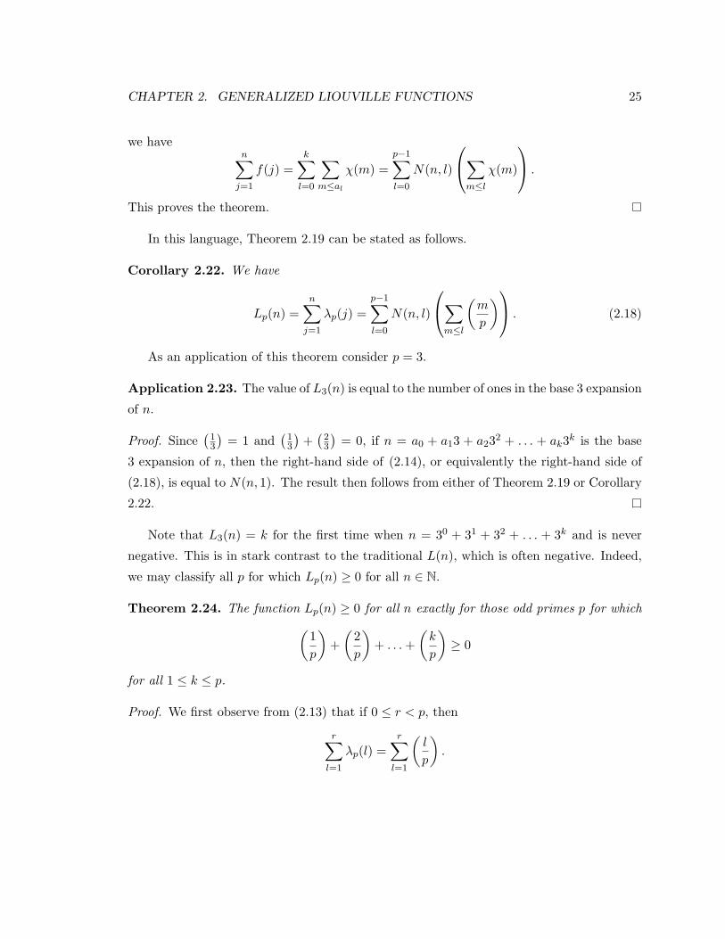
In this language, Theorem 2.19 can be stated as follows.
Corollary 2.22. We have
Lp(n) =n∑j=1
λp(j) =p−1∑l=0
N(n, l)
∑m≤l
(m
p
) . (2.18)
As an application of this theorem consider p = 3.
Application 2.23. The value of L3(n) is equal to the number of ones in the base 3 expansion
of n.
Proof. Since(
13
)= 1 and
(13
)+(
23
)= 0, if n = a0 + a13 + a232 + . . . + ak3k is the base
3 expansion of n, then the right-hand side of (2.14), or equivalently the right-hand side of
(2.18), is equal to N(n, 1). The result then follows from either of Theorem 2.19 or Corollary
2.22.
Note that L3(n) = k for the first time when n = 30 + 31 + 32 + . . . + 3k and is never
negative. This is in stark contrast to the traditional L(n), which is often negative. Indeed,
we may classify all p for which Lp(n) ≥ 0 for all n ∈ N.
Theorem 2.24. The function Lp(n) ≥ 0 for all n exactly for those odd primes p for which(1p
)+(
2p
)+ . . .+
(k
p
)≥ 0
for all 1 ≤ k ≤ p.
Proof. We first observe from (2.13) that if 0 ≤ r < p, then
r∑l=1
λp(l) =r∑l=1
(l
p
).

CHAPTER 2. GENERALIZED LIOUVILLE FUNCTIONS 26
Let n = a0 + a1p+ · · ·+ akpk be the base p expansion of n. From Theorem 2.19,
n∑l=1
λp(l) =a0∑l=1
λp(l) +a1∑l=1
λp(l) + . . .+ak∑l=1
λp(l)
=a0∑l=1
(l
p
)+
a1∑l=1
(l
p
)+ . . .+
ak∑l=1
(l
p
)because all aj are between 0 and p− 1. The result then follows.
Corollary 2.25. For n ∈ N, we have
0 ≤ L3(n) ≤ [log3 n] + 1.
Proof. This follows from Theorem 2.24, Application 3.21, and the fact that the number of
1’s in the base three expansion of n is ≤ [log3 n] + 1.
As a further example, let p = 5.
Corollary 2.26. The value of L5(n) is equal to the number of 1’s in the base 5 expansion
of n minus the number of 3’s in the base 5 expansion of n. Also for n ≥ 1,
|L5(n)| ≤ [log5 n] + 1.
Recall from above, that L3(n) is always nonnegative, but L5(n) isn’t. Also L5(n) = k
for the first time when n = 50 + 51 + 52 + . . .+ 5k and L5(n) = −k for the first time when
n = 3 · 50 + 3 · 51 + 3 · 52 + . . .+ 3 · 5k.
Remark 2.27. The reason for specification of the primes p in the preceding two corollaries
is that, in general, it’s not always the case that |Lp(n)| ≤ [logp n] + 1.
We now return to our classification of primes for which Lp(n) ≥ 0 for all n ≥ 1.
Definition 2.28. Denote by L+, the set of primes p for which Lp(n) ≥ 0 for all n ∈ N.
We have found by computation that the first few values in L+ are
L+ = (3, 7, 11, 23, 31, 47, 59, 71, 79, 83, 103, 131, 151, 167, 191, 199, 239, 251 . . .).
By inspection, L+ doesn’t seem to contain any primes p, with p ≡ 1 (mod 4). This is not
a coincidence, as demonstrated by the following theorem.
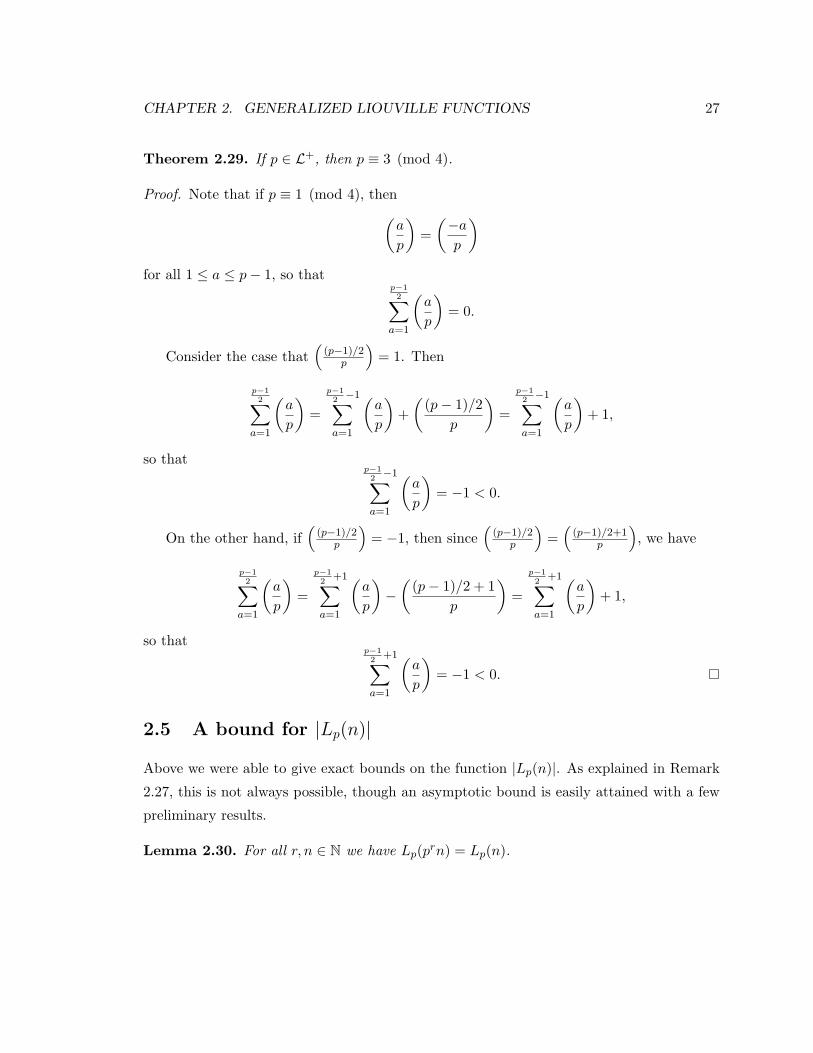
CHAPTER 2. GENERALIZED LIOUVILLE FUNCTIONS 27
Theorem 2.29. If p ∈ L+, then p ≡ 3 (mod 4).
Proof. Note that if p ≡ 1 (mod 4), then(a
p
)=(−ap
)for all 1 ≤ a ≤ p− 1, so that
p−12∑
a=1
(a
p
)= 0.
Consider the case that(
(p−1)/2p
)= 1. Then
p−12∑
a=1
(a
p
)=
p−12−1∑
a=1
(a
p
)+(
(p− 1)/2p
)=
p−12−1∑
a=1
(a
p
)+ 1,
so thatp−12−1∑
a=1
(a
p
)= −1 < 0.
On the other hand, if(
(p−1)/2p
)= −1, then since
((p−1)/2
p
)=(
(p−1)/2+1p
), we have
p−12∑
a=1
(a
p
)=
p−12
+1∑a=1
(a
p
)−(
(p− 1)/2 + 1p
)=
p−12
+1∑a=1
(a
p
)+ 1,
so thatp−12
+1∑a=1
(a
p
)= −1 < 0.
2.5 A bound for |Lp(n)|
Above we were able to give exact bounds on the function |Lp(n)|. As explained in Remark
2.27, this is not always possible, though an asymptotic bound is easily attained with a few
preliminary results.
Lemma 2.30. For all r, n ∈ N we have Lp(prn) = Lp(n).

CHAPTER 2. GENERALIZED LIOUVILLE FUNCTIONS 28
Proof. For i = 1, . . . , p − 1 and k ∈ N, λp(kp + i) = λp(i). For k ∈ N, this relation
immediately gives that Lp(p(k + 1)− 1)− Lp(pk) = 0, since Lp(p− 1) = 0. Thus
Lp(prn) =prn∑k=1
λp(k) =pr−1n∑k=1
λp(pk) =pr−1n∑k=1
λp(p)λp(k) =pr−1n∑k=1
λp(k) = Lp(pr−1n).
The lemma follows immediately.
Theorem 2.31. The maximum value of |Lp(n)| for n < pk occurs at n = k · σ(pk−1) with
value
maxn<pk
|Lp(n)| = k ·maxn<p|Lp(n)|,
where σ(n) is the sum of the divisors of n.
Proof. This follows directly from Lemma 2.30.
Corollary 2.32. If p is an odd prime, then |Lp(n)| log n; furthermore,
maxn≤x|Lp(x)| log x.
This last corollary begs the question: what can be said about the growth of∣∣∣∑n≤x f(n)
∣∣∣for any function f ∈ F(−1, 1)? Presumably this quantity is unbounded for all such f ,
though this is presently unknown.

Chapter 3
Mahler’s method via two examples
Before considering values and power series of more general functions in F(−1, 1), we
present two detailed examples using Mahler’s transcendence methods. The proofs here were
inspired by Dekking’s proof of the transcendence of the Thue–Morse number [34].
The two examples discussed here concern power series, F (z) ∈ C[[z]], which satisfy two
very different types of functional equations similar to
(k ≥ 2) F (zk) = R(z)F (z) and F (zk) = F (z) +R(z),
where R(z) ∈ Z(z).
3.1 Stern’s diatomic sequence
The Stern sequence, sometimes called Stern’s diatomic sequence, (a(n))n≥0 is given by
a(0) = 0, a(1) = 1, and when n ≥ 1, by
a(2n) = a(n) and a(2n+ 1) = a(n) + a(n+ 1).
Properties of this sequence have been studied by many authors; for references see [36]. The
Stern sequence is A002487 in Sloane’s list (see http://www.research.att.com/∼njas/sequences/A000108). In the article cited above, Dilcher and Stolarsky introduced and
studied a polynomial analogue of the Stern sequence, defined by a(0;x) = 0, a(1;x) = 1,
and when n ≥ 1, by
a(2n;x) = a(n;x2) and a(2n+ 1;x) = x a(n;x2) + a(n+ 1;x2).
29

CHAPTER 3. MAHLER’S METHOD VIA TWO EXAMPLES 30
We call a(n;x) the nth Stern polynomial. Denote by A(z) and A(x, z) the generating
functions of the Stern sequence and Stern polynomials, respectively.
In this section, we prove that these generating functions are transcendental.
There are some special subsequences of (a(n))n≥0 of interest. It is known (see Lehmer
[70] and Lind [71]) that the maximum value of a(m) in the interval 2n−2 ≤ m ≤ 2n−1 is the
nth Fibonacci number Fn and that this maximum occurs at
m =13
(2n − (−1)n) and m =13
(5 · 2n−2 + (−1)n).
Dilcher and Stolarsky [35] set
αn :=13
(2n − (−1)n) (n ≥ 0), βn :=13
(5 · 2n−2 + (−1)n) (n ≥ 2),
and define for n ≥ 0
fn(q) := a(αn; q)
and for n ≥ 2
fn(q) := a(βn; q).
Throughout the paper [35] the authors study properties of fn and fn, finding functional
equations and other such relationships. They are particularly concerned with the functions
F and G defined as follows.
Definition 3.1. For complex q with |q| < 1 we define
F (q) : = limn→∞
f2n(q) = limn→∞
f2n+1(q)
= 1 + q + q2 + q5 + q6 + q8 + q9 + q10 + q21 + q22 + q24 + · · · ,
G(q) : = limn→∞
f2n+1(q) = limn→∞
f2n(q)
= 1 + q + q3 + q4 + q5 + q11 + q12 + q13 + q16 + q17 + q19 + · · · .
In a remark in [35], Dilcher and Stolarsky ask about the transcendence of F and G but
make no conclusions. We resolve this question: these functions are transcendental.

CHAPTER 3. MAHLER’S METHOD VIA TWO EXAMPLES 31
3.1.1 Transcendence of A(z)
Recall that A(z) :=∑
n≥0 a(n)zn. Using the definition of the Stern sequence, we have
A(z) =∑n≥0
a(2n)z2n +∑n≥0
a(2n+ 1)z2n+1
=∑n≥0
a(n)z2n +∑n≥0
a(n)z2n+1 +∑n≥0
a(n+ 1)z2n+1
= A(z2) + zA(z2) +∑n≥0
a(n)z2n−1
= A(z2)(
1 + z +1z
),
which gives the following lemma (this result can also be derived from (2.9) in [36]).
Lemma 3.2. If A(z) is the generating function of the Stern sequence, then
A(z2) = A(z)(
z
z2 + z + 1
).
Theorem 3.3. The function A(z) is transcendental over C(z).
Proof. Towards a contradiction, suppose that A(z) is algebraic and satisfies, say,
qn(z)A(z)n + qn−1(z)A(z)n−1 + · · ·+ q0(z) = 0 (3.1)
where qi(z) ∈ C[z], gcd(qn(z), qn−1(z), . . . , q0(z)) = 1, and n is chosen minimally. Using the
functional equation, we have
0 =n∑k=0
qk(z2)A(z2)k =n∑k=0
qk(z2)A(z)k(
z
z2 + z + 1
)k,
and upon multiplying by (z2 + z + 1)n we obtain
0 =n∑k=0
qk(z2)(z2 + z + 1)n−kzkA(z)k.
Thus
0 = znqn(z2)n∑k=0
qk(z)A(z)k − qn(z)n∑k=0
qk(z2)(z2 + z + 1)n−kzkA(z)k
=n∑k=0
[qn(z2)qk(z)zn − qn(z)qk(z2)(z2 + z + 1)n−kzk
]A(z)k. (3.2)

CHAPTER 3. MAHLER’S METHOD VIA TWO EXAMPLES 32
The coefficient of A(z)n in (3.2) is
qn(z2)qn(z)zn − qn(z)qn(z2)zn = 0,
so that
0 =n−1∑k=0
[qn(z2)qk(z)zn − qn(z)qk(z2)(z2 + z + 1)n−kzk
]A(z)k.
The minimality of n gives
qn(z2)qk(z)zn = qn(z)qk(z2)(z2 + z + 1)n−kzk (3.3)
for k = 0, 1, . . . , n− 1.
Recall that gcd(qn(z), qn−1(z), . . . , q0(z)) = 1, so that gcd(qn(z2), qn−1(z2), . . . , q0(z2)) =
1. Denote the primitive cube roots of unity by ω and ω2. We have (z−ω)(z−ω2) = z2+z+1.
Equation (3.3) gives for all i = 0, 1, . . . , n that both
z − ω | qi(z) ⇐⇒ z − ω2 | qi(z2) (3.4)
and
z − ω2 | qi(z) ⇐⇒ z − ω | qi(z2). (3.5)
Denote by Na(p(z)) the multiplicity of the root z = a of p(z). Also note that for all
i = 0, 1, . . . , n the equations (3.4) and (3.5) give
Nω(qi(z)) = Nω2(qi(z2)) and Nω(qi(z2)) = Nω2(qi(z)).
Then (3.3), (3.4) and (3.5) give the system of equations
Nω(qn(z2)) +Nω(qk(z)) = Nω(qn(z)) +Nω(qk(z2)) + n− k (3.6)
Nω(qn(z)) +Nω(qk(z2)) = Nω(qn(z2)) +Nω(qk(z)) + n− k. (3.7)
Substitution of (3.5) into (3.4) gives n = k, a contradiction. Therefore, A(z) is transcen-
dental.
We proceed to show that the values of A(z) at algebraic z ∈ C are transcendental. We
use a theorem of Mahler [73], as taken from Nishioka’s book [83]. For completeness, a full
proof of this theorem is contained in Appendix A. Here I is the set of algebraic integers over
CHAPTER 3. MAHLER’S METHOD VIA TWO EXAMPLES 33
Q, K is an algebraic number field, IK = K ∩I, and f(z) ∈ K[[z]] with radius of convergence
R > 0 satisfying the functional equation for an integer d > 1,
f(zd) =∑m
i=0 bi(z)f(z)i∑mi=0 ci(z)f(z)i
, m < d, bi(z), ci(z) ∈ IK [z],
and ∆(z) := Res(B,C) is the resultant of B(u) =∑m
i=0 bi(z)ui and C(u) =
∑mi=0 ci(z)u
i as
polynomials in u.
Theorem 3.4 (Mahler [73]). Assume that f(z) is not algebraic over K(z). If α is an
algebraic number with 0 < |α| < min1, R and ∆(αdk) 6= 0 (k ≥ 0), then f(α) is transcen-
dental.
Using Mahler’s Theorem we prove
Theorem 3.5. If α 6= 0 is an algebraic number with 0 < |α| < 1, then A(α) is transcendental
over Q.
Proof. Let α 6= 0 be an algebraic number with 0 < |α| < 1. Lemma 3.2 gives
A(z2) =zA(z)
z2 + z + 1,
so that the resultant (in the variable u) is
∆(α2k) = Res(zu, z2 + z + 1)
∣∣∣z=α2k
= α2k+1+ α2k
+ 1,
which is non–zero for every k ≥ 0. The result follows.
3.1.2 Transcendence of A(x, z)
Theorem 3.6. The function A(x, z) is transcendental.
To prove Theorem 3.6 we need the following straightforward lemma concerning values
of algebraic functions.
Lemma 3.7. If f is a power series expansion of an algebraic function, and α 6= 0 is an
algebraic number within the radius of convergence of f , then f(α) is algebraic.
Proof. Suppose that f is a power series expansion of an algebraic function of degree n with∑nk=0 qk(z)f(z)k = 0, and α 6= 0 is an algebraic number within the radius of convergence
of f . Since the qk(z) are polynomials, qk(α) is an element in the required ring/field and so
f(α) satisfies the algebraic equation∑n
k=0 qk(α)f(α)k = 0. Thus f(α) is algebraic.

CHAPTER 3. MAHLER’S METHOD VIA TWO EXAMPLES 34
Proof of Theorem 3.6. From the definitions of the Stern sequence and Stern polynomials,
we have a(n; 1) = a(n) so that
A(1, z) = A(z).
Lemma 3.7 tells us that to prove the transcendence of A(x, z) we need only find algebraic
values of x and z so that at this value of A(x, z) is not algebraic.
Consider x = 1 and z = 12 . Then
A
(1,
12
)= A
(12
),
which by Theorem 3.5 is not algebraic, and we have proven the desired result.
3.1.3 Transcendence of F (q) and G(q)
We now turn to the functions F (q) and G(q) as introduced in Definition 3.1.
Theorem 3.8. The functions F (q) and G(q) defined above are transcendental over Q(z).
To prove this theorem we will need a couple of results from elsewhere. The first is a
theorem of Fatou [48] and the second from Dilcher and Stolarsky [35].
Theorem 3.9 (Fatou, 1906). A power series whose coefficients take only finitely many
values that belong to Q is either rational or transcendental.
Proposition 3.10 (Dilcher and Stolarsky [35]). The coefficients of fn(q) and fn(q) are 0
or 1, and for k ≥ 1 we have
deg f2k(q) = α2k−1 − 1, deg f2k+1(q) = α2k,
deg f2k(q) = β2k−1, deg f2k+1(q) = β2k − 1,
where αn and βn are as defined previously.
Fatou’s theorem is very useful in transcendence proofs. Many different proofs have been
given, the first by Fatou in 1906 [48], Allouche in 1999 [3] and again by Borwein and Coons
in 2009 [16], whose proof is presented in Chapter 4 of this thesis.
Proof of Theorem 3.8. Recall that G(q) = limn→∞ f2k+1(q). Proposition 5.3 gives
deg f2k+1(q) = α2k =13
(22k − 1).
CHAPTER 3. MAHLER’S METHOD VIA TWO EXAMPLES 35
The number of terms of f2k+1 is
f2k+1(1) = F2k+1 = [ϕ2k+1],
where the second equality is true for k ≥ 2, [x] represents the greatest integer less than or
equal to x, and ϕ is the golden ratio. It is important to note that the degree is growing
much faster than the number of terms; this property along with Fatou’s theorem is enough
to give the result.
Consider the degree of f2k+1 as k grows. We have
deg f2k+3(q)− deg f2k+1(q) = α2k+2 − α2k = 22k.
If we write the polynomial
f2k+3(q)− f2k+1(q) = εα2k+1qα2k+1 + εα2k+2q
α2k+2 + · · ·+ εα2k+2qα2k+2 ,
then the proportion of εis that are 1 is
[ϕ2k+2]22k
which approaches 0 as k goes to infinity.
Let h be a given positive integer. Then there exists a k := k(h) for which
[ϕ2k+2]22k
<1h2.
Thus, for this k, the polynomial f2k+3(q)− f2k+1(q) contains at least h consecutive εis with
εi = 0.
Now pick q = 12 . Then G(1/2) is a binary number with (in binary notation)
G(1/2) = ε0.ε1ε2ε3ε4ε5 . . . = 1.1100110111 . . . .
The previous paragraph tells us that there are arbitrarily long runs of zeros in the binary
expansion of G(1/2). Since deg f2k+1(q)→∞ with k, there are infinitely many ones in the
binary expansion of G(1/2) and so G(1/2) is an irrational number. Hence G(q) is not a
rational function. Application of Fatou’s theorem gives the desired result.

CHAPTER 3. MAHLER’S METHOD VIA TWO EXAMPLES 36
3.2 Golomb’s series
Golomb proved in [49] that the values of the functions∑n≥0
z2n
1 + z2n and∑n≥0
z2n
1− z2n
are irrational at z = 1t for t = 2, 3, 4, . . . , the interesting special case of which is that the
sum of the reciprocals of the Fermat numbers is irrational. Schwarz [88] has given results
on series of the form
Gk(z) :=∑n≥0
zkn
1− zkn .
In particular, he proved that if k, t and b are integers satisfying
k ≥ 2, t ≥ 2, and 1 ≤ b < t1−1/k,
then the number
Gk(bt−1) =∑n≥0
bkn
tkn − bkn
is irrational. Schwarz also showed that for k, t, b ∈ N with k > 2, t ≥ 2 and 1 ≤ b < t1−5/2k
the number Gk(bt−1) is transcendental. The case k = 2 proved to be more difficult, though
he was able to show that for an integer t ≥ 2 the number G2(t−1) is not algebraic of the
second degree.
Schwarz also remarks in [88] that, “the irrationality of∑n≥0
bkn(tk
n+ bk
n)−1
for k > 2 is unsettled.” In our notation, this is Fk(bt−1).
Recently, Duverney [38] has proven the transcendence of G2(t−1) for integers t ≥ 2
and extended Schwarz’s transcendence results for the case k = 2. He proved the following
theorem.
Theorem 3.11 (Duverney [38]). Let a ≥ 2 be an integer and let bn be a sequence of integers
satisfying |bn| = O(η−2n) for every η ∈ (0, 1). Suppose that a2n
+ bn 6= 0 for every n ∈ N.Then the number
S =∑n≥0
1a2n + bn
is transcendental.
CHAPTER 3. MAHLER’S METHOD VIA TWO EXAMPLES 37
We extend Schwarz’s results further (to the best possible); in particular, we prove that
for all k ≥ 2 the series Gk(z) =∑
n≥0 zkn
(1 − zkn)−1 is transcendental for all algebraic
numbers z with |z| < 1. We also prove the same result for Fk(z) =∑
n≥0 zkn
(1 + zkn)−1
which settles the irrationality question of Schwarz’s remark. These results were known to
Mahler (see [73, 74, 75, 76]), though our proofs of the function’s transcendence are new
and elementary, coming from the proof of our main result; no linear algebra or differential
calculus is used.
The main result of this section is that a non–zero power series F (z) ∈ C[[z]] satisfying
F (zd) = F (z) +A(z)B(z)
,
where A(z), B(z) ∈ C[z] with A(z) 6= 0 and degA(z),degB(z) < d is transcendental over
C(z). This extends a theorem of Nishioka [82] that states that F (z) is either transcendental
or rational.
3.2.1 A general transcendence theorem
Nishioka [82] has shown
Theorem 3.12 (Nishioka [82]). Suppose that F (z) ∈ C[[z]] satisfies one of the following for
an integer d > 1.
(i) F (zd) = ϕ(z, F (z)),
(ii) F (z) = ϕ(z, F (zd)),
where ϕ(z, u) is a rational function in z, u over C. If F (z) is algebraic over C(z), then
F (z) ∈ C(z).
Nishioka’s proof of Theorem 3.12 relies on deep ideas from algebraic number theory.
In this section we provide an elementary proof of a special case of Theorem 3.12. In this
special case, we are able to refine the conclusion by eliminating the possibility of F (z) being
a rational function.
Theorem 3.13. If F (z) is a power series in C[[z]] satisfying
F (zd) = F (z) +A(z)B(z)
,
where d ≥ 2, A(z), B(z) ∈ C[z] with A(z) 6= 0 and degA(z),degB(z) < d, then F (z) is
transcendental over C(z).

CHAPTER 3. MAHLER’S METHOD VIA TWO EXAMPLES 38
Proof. Suppose that the power series F (z) is algebraic, and satisfies
n∑r=0
qr(z)F (z)r ≡ 0 (3.8)
where the qr(z) are rational functions with qn(z) = 1 and n ≥ 1 is chosen minimally. The
notation ≡ is used to mean identically equal.
Substituting zd into (3.8) and using the functional relation gives
0 ≡n∑r=0
qr(zd)F (zd)r =n∑r=0
qr(zd)(F (z) +
A(z)B(z)
)r.
Without loss of generality, suppose B(z) is monic. Multiplying by B(z)n to clear fractions
as well as an application of the binomial theorem yields
0 ≡n∑r=0
qr(zd)B(z)n−r(B(z)F (z) +A(z)
)r=
n∑r=0
qr(zd)B(z)n−rr∑j=0
(r
j
)B(z)jF (z)jA(z)r−j . (3.9)
Taking the difference between (3.9) and B(z)n times (3.8) gives
Q(z) :=n∑r=0
qr(zd)B(z)n−rr∑j=0
(r
j
)B(z)jF (z)jA(z)r−j −B(z)n
n∑r=0
qr(z)F (z)r ≡ 0. (3.10)
Note that we may also write
Q(z) =n∑
m=0
hm(z)F (z)m ≡ 0,
for some polynomials h0(z), . . . , hn(z) ∈ C[z].
We determine hn(z). The only term in Q(z) that can contribute to the coefficient of
F (z)n is the term with r = n of the sum (3.10), which recalling that qn(z) = 1 is
n∑j=0
(n
j
)B(z)jF (z)jA(z)n−j −B(z)nF (z)n,
and only the j = n term here contributes. Hence
hn(z) =(n
n
)B(z)nA(z)n−n −B(z)n = 0,

CHAPTER 3. MAHLER’S METHOD VIA TWO EXAMPLES 39
so that Q(z) =∑n−1
m=0 hm(z)F (z)m ≡ 0. Since n was chosen minimally, hm(z) ≡ 0 for all
m = 0, 1, . . . , n− 1.
Using (3.10) we have that
hm(z) =n∑
r=m
(r
m
)qr(zd)B(z)n−r+mA(z)r−m −B(z)nqm(z).
Since hn−1(z) ≡ 0 this gives
n∑r=n−1
(r
n− 1
)qr(zd)B(z)n−r+(n−1)A(z)r−(n−1) = B(z)nqn−1(z)
so that with the removal of shared factors, recalling qn(z) = 1, we have the identity
qn−1(zd)B(z) + nA(z) = B(z)qn−1(z). (3.11)
Write qn−1(z) = α(z)β(z) where α(z), β(z) ∈ C[z] with gcd(α(z), β(z)) = 1 and β(z) monic.
Denote g(z) := gcd(β(z), β(zd)), so that β(z)g(z) ,
β(zd)g(z) ∈ C[z] and hence gcd
(β(z)g(z) ,
β(zd)g(z)
)= 1.
Then (3.11) becomes(β(z)g(z)
)α(zd)B(z) + n
(β(z)g(z)
)β(zd)A(z) =
(β(zd)g(z)
)B(z)α(z). (3.12)
Thus β(z)g(z)
∣∣B(z). Also, since β(z)g(z)β(zd) = β(z)β(zd)
g(z) we have β(zd)g(z)
∣∣B(z).
Equation (3.11) yields β(zd) | β(z)α(zd)B(z), which implies that
d · deg β(z) ≤ deg β(z) + degB(z) < deg β(z) + d.
Hence
0 ≤ deg β(z) < 1 +1
d− 1.
Since d ≥ 2, either deg β(z) = 0 or deg β(z) = 1.
Suppose deg β(z) = 0. Hence β(z) = β(zd) ∈ C; write β := β(z). Now (3.12) becomes
α(zd)B(z) + nβA(z) = B(z)α(z). (3.13)
Thus B(z) | nβ which gives degB(z) = 0. Write B := B(z). Thus (3.13) becomes
α(zd)B + nβA(z) = Bα(z), (3.14)
which implies that d · degα(z) = degA(z) < d so that degα(z) = 0. Eq. (3.14) and
degα(z) = 0 imply that A(z) = 0 which is impossible.

CHAPTER 3. MAHLER’S METHOD VIA TWO EXAMPLES 40
Now suppose deg β(z) = 1 and write β(z) = z− β. Comparing degrees in (3.12) implies
that degα(z) ≤ 1.
Recall that both β(z)g(z)
∣∣B(z) and β(zd)g(z)
∣∣B(z). Since gcd(β(z)g(z) ,
β(zd)g(z)
)= 1, we have that(
β(z)g(z) ·
β(zd)g(z)
) ∣∣B(z). The bound degB(z) < d and deg g(z) = 1 give g(z) = β(z). Sinceβ(zd)g(z) = β(zd)
β(z)
∣∣B(z) and both β(z) and B(z) are monic with degB(z) < d, we have
β(zd)β(z)
= B(z).
Suppose that degα(z) = 1. Write α(z) = δ(z − α) and note that β 6= α. In this case,
solving (3.12) for A(z) gives
A(z) =δ(β − α)z(zd−1 − 1)
n(z − β)2∈ C[z].
Since A(z) ∈ C[z] we have that (z − β)2|(zd−1 − 1), which we may rewrite as
(z − β)2
∣∣∣∣∣d−2∏k=0
(z − e2πi k
d−1
).
This is not possible since e2πi ld−1 6= e2πi m
d−1 for any l,m with 0 ≤ l < m ≤ d − 2 (that is,
(d− 1)–th roots of unity are distinct); hence degα(z) = 0.
If degα(z) = 0, write α := α(z). Then writing β(z) = z − β and solving (3.12) for A(z)
we have that
A(z) =αz(zd−1 − 1)n(z − β)2
/∈ C[z],
which contradicts that A(z) ∈ C[z].
Corollary 3.14. There is no rational function F (z) in C(z) satisfying
F (zd) = F (z) +A(z)B(z)
,
where d ≥ 2, A(z), B(z) ∈ C[z] with A(z) 6= 0 and degA(z),degB(z) < d.
3.2.2 The series Gk(z) and Fk(z)
To prove the transcendence results surrounding Gk(z) and Fk(z), we apply Theorem 3.13
as well as Theorem 3.4.

CHAPTER 3. MAHLER’S METHOD VIA TWO EXAMPLES 41
Consider the functional equation f(zk) = f(z)− z1−z with k ≥ 2. Repeated application
yields
f(zkm
) = f(zkm−1
)− zkm−1
1− zkm = f(z)−m∑n=1
zkm−n
1− zkm−n .
Changing the index and setting Wm(z) :=∑m−1
n=0zkn
1−zkn gives
f(z) = f(zkm
) +Wm(z).
In the region |z| < 1, we have
f(z) = limm→∞
[f(zk
m) +Wm(z)
]=∑n≥0
zkn
1− zkn = Gk(z).
This proves the following lemma.
Lemma 3.15. For |z| < 1, the function Gk(z) satisfies the functional equation
Gk(zk) = Gk(z) +z
z − 1.
As a corollary of Theorem 3.13, we have
Corollary 3.16. For k ≥ 2, the function Gk(z) is transcendental over C(z).
To get the transcendence of the associated numbers, we use Mahler’s Theorem.
Proposition 3.17. If k ≥ 2 and α is algebraic with 0 < |α| < 1, then Gk(α) is transcen-
dental over Q.
Proof. Lemma 3.15 gives the functional equation
Gk(zk) =(1− z)Gk(z)− z
1− z,
so that, in the language of Theorem 3.4, we have
A(u) = (1− z)u− z and B(u) = 1− z,
m = 1 < k = d, and ai(z), bi(z) ∈ IK [z]. Since B(u) is a constant polynomial in u,
∆(z) := Res(A,B) = 1− z.

CHAPTER 3. MAHLER’S METHOD VIA TWO EXAMPLES 42
Let |α| < 1 be algebraic; it is immediate that
∆(αkn) = 1− αkn 6= 0 (n ≥ 0).
Since Gk(z) is not algebraic over C(z) (as supplied by Corollary 3.16), applying Theorem
3.4, we have that Gk(α) is transcendental over Q.
Corollary 3.18. If k, b, t ∈ N with k ≥ 2 and 0 < b < t, then the number Gk(bt−1) is
transcendental over Q.
Proof. Set α = b/t in Theorem 3.17.
We turn now to the series
Fk(z) =∑n≥0
zkn
1 + zkn .
Similar to Gk(z), the function Fk(z) satisfies a functional equation,
Fk(zk) = Fk(z)−z
z + 1.
Theorem 3.13 yields
Corollary 3.19. The function Fk(z) is transcendental over C(z).
As before, Mahler’s Theorem gives
Proposition 3.20. For k ≥ 2 and z = α an algebraic number with 0 < |α| < 1, Fk(α) is
transcendental over Q.
Corollary 3.21. If k, b, t ∈ N with k ≥ 2 and 1 ≤ b < t, then the number Fk(bt−1) is
transcendental over Q.
Remark 3.22. For some more recent work concerning results like Nishioka’s Theorem
3.12, for more general algebraic number fields, see [40]; this paper also contains a number
of current references to results in this area. Also, concerning functions similar to Gk(z)
and Fk(z) above, Duverney, Kanoko, and Tanaka [39] have given a complete classification
of those series
f(z) :=∑k≥0
akzdk
1 + bzdk + cz2dk ∈ C[[z]]
that are transcendental over C(z) where C is a field of characteristic 0, d ≥ 2, and a, b, c ∈ Cwith a 6= 0.
Chapter 4
Irrationality and transcendence
In this chapter we return to our investigation of functions f ∈ F(−1, 1) by considering
formal power series with coefficients f(n) as well as the values of power series whose coeffi-
cients come from a certain subset of F(−1, 1). The results of this chapter are taken from
two joint publications ([15] and [16]) with Peter Borwein.
4.1 Formal power series
In 1945, Duffin and Schaeffer [37] proved that
Theorem 4.1 (Duffin and Schaeffer [37]). A power series that is bounded in a sector and
has coefficients from a finite subset is a rational function.
Their proof is relatively indirect. In [17], Borwein, Erdelyi, and Littman gave a shorter
direct proof.
The theorem of Duffin and Schaeffer is a generalization of a result of Szego who proved
in 1922 that a power series whose coefficients assume only finitely many values and which
can be extended analytically beyond the unit circle is a rational function.
In 1906, Fatou [48] proved, and in 1999, Allouche [3] reproved using a deep result of
Cobham [25], that
Theorem 4.2 (Fatou [48]). A power series whose coefficients take only finitely many ra-
tional values is either rational or transcendental.
In this section, we give a new proof of Fatou’s theorem and apply it to show that if
f ∈ F(−1, 1) and f is not identically 1, then∑
n≥1 f(n)zn is transcendental over Z(z).
43

CHAPTER 4. IRRATIONALITY AND TRANSCENDENCE 44
As a specific example, we show the transcendence of the series∑
n≥1 λ(n)zn. We also use
Fatou’s theorem to show that∑
n≥1 µ(n)zn. Here λ and µ are the Liouville and Mobius
functions, respectively.
We will need the following quantitative version of the Fundamental Theorem of Algebra
[18, Theorem 1.2.1].
Lemma 4.3. The polynomial
p(z) := anzn + an−1z
n−1 + · · ·+ a0 ∈ C[z], an 6= 0
has exactly n zeros in C. These all lie in the open disk of radius r centered at the origin,
where
r := 1 + max0≤k≤n−1
|ak||an|
.
Proof of Theorem 4.2. Suppose that f(z) is a power series with coefficients that take only
finitely many rational values, and satisfies
an(z)f(z)n + an−1(z)f(z)n−1 + · · ·+ a0(z) = 0
where each ai(z) is a polynomial with integer coefficients. Since the leading coefficient
an(z) of this polynomial equation is a polynomial, it has finitely many zeros. Hence there
is a sector S of the open unit disk where |an(z)| is bounded away from zero uniformly. The
modulus of each other coefficient ak(z) is clearly uniformly bounded above on S. Now apply
Lemma 4.3 to conclude that |f(z)| is bounded on S, so the result of Duffin and Schaeffer
applies.
As before, denote by µ the Mobius function, and by λ the Liouville function. Recall that
λ is the unique completely multiplicative function defined by λ(p) = −1 for all primes p.
In [8], it is shown that the formal power series∑
n≥1 λ(n)zn,∑
n≥1 µ(n)zn ∈ Z[[z]] are
irrational over Z(z) (along with various other multiplicative functions). We proceed by
proving that these two power series are transcendental over Z(z). The transcendence of∑n≥1 λ(n)zn is stated as a corollary to the following general theorem.
Theorem 4.4. Let f : N→ −1, 1 be a completely multiplicative function with the property
that for some prime p, f(p) = −1. Then∑
n≥1 f(n)zn ∈ Z[[z]] is transcendental over Z(z).

CHAPTER 4. IRRATIONALITY AND TRANSCENDENCE 45
Proof. In light of Theorem 4.2, we need only demonstrate that for a completely multiplica-
tive function f : N→ −1, 1 such that there is a prime p for which f(p) = −1, the sequence
of values of f is not eventually periodic. This would show that∑
n≥1 f(n)2−n is irrational.
Denote the sequence of values of f by F.
Towards a contradiction, suppose that F is eventually periodic, say the sequence is
periodic after the M–th term and has period k. Now there is an N ∈ N such that for all
n ≥ N , we have nk > M . Let p be a prime for which f(p) = −1. Then
f(pnk) = f(p)f(nk) = −f(nk).
But pnk ≡ nk (mod k), a contradiction to the eventual k–periodicity of F.
Corollary 4.5. If λ is the Liouville function, then the series∑
n≥1 λ(n)zn ∈ Z[[z]] is
transcendental over Z(z).
Note that Theorem 4.4 does not apply directly to the Mobius function because µ is not
completely multiplicative. Recall from the definition that if p2 | n for any prime p, then
µ(n) = 0. From this fact alone one may use the Chinese Remainder Theorem to show that
sequence of values of the Mobius function contains arbitrarily long runs of zeroes. This in
turn gives the irrationality of∑
n≥1 µ(n)zn at z = 13 , and hence the following corollary to
Theorem 4.2.
Corollary 4.6. If µ is the Mobius function, then the series∑
n≥1 µ(n)zn ∈ Z[[z]] is tran-
scendental over Z(z).
The transcendence of the series∑
n≥1 f(z)zn over Z(z) for f equal to each of the multi-
plicative functions τk, σk, and ϕ was shown by Yazdani [98]; the case f = µ was previously
treated by Allouche [3] using a deep result of Cobham [26].
While transcendence results on power series are readily available, there are many open
questions concerning their special values. Erdos [43] was interested in the transcendence
and irrationality of both∑
n≥1 τ(n)2−n and∑
n≥1 ϕ(n)2−n. The irrationality of the first
sum was shown by Borwein [11]; the transcendence is not yet known. Questions regarding
the algebraic character of∑
n≥1 ϕ(n)2−n remain open. Nesterenko [79] has shown that the
number ∑n≥1
λ(n)2n − 1
CHAPTER 4. IRRATIONALITY AND TRANSCENDENCE 46
is transcendental, but the transcendence of its close relative,∑
n≥1 λ(n)2−n remains elusive.
Using Mahler’s method, as described in Chapter 3, in the next section we approach the
transcendence of values of power series whose coefficients are given by certain functions in
F(−1, 1).
4.2 Values of power series
Denote the sequence of λ values by L and recall that the Liouville number l is the binary
number
l :=∑n≥1
(1 + λ(n)
2
)12n
= 0.100101001100011100001 . . . .
Properties of the number l are properties of the sequence L. One noteworthy property is
that l is irrational.
Theorem 4.7. The Liouville number is not rational.
Proof. See the proof of Theorem 4.4.
The irrationality of l tells us that the sequence L is not eventually periodic. A fun-
damental question arises, which at present we are unable to answer. We believe that l is
transcendental, though this seems currently unapproachable. For other completely multi-
plicative functions like λ, we can decide transcendence.
In this section, we consider a subset of F(−1, 1).As an example, let g be the completely multiplicative function defined on primes p by
gp =
−1 if p ≡ 3(mod 4)
1 otherwise.
As the function g takes the value −1 on those primes which are rational Gaussian primes,
we call g the Gaussian Liouville function. Denote by G the sequence of values of g, and
define
γ :=∑n≥1
(1 + gn
2
)12n
as the Gaussian Liouville number. One can show that gn = (−1/n) where (·/n) is the Jacobi
symbol modulo n. The Gaussian Liouville number is easily seen to be irrational. Indeed, it
is a corollary to the following generalization of Theorem 4.7.

CHAPTER 4. IRRATIONALITY AND TRANSCENDENCE 47
Theorem 4.8. Suppose that f : N → −1, 1 is a completely multiplicative function, with
f(p) = −1 for at least one prime p, and F its sequence of values. If ϕ :=∑
n≥1
(1+f(n)
2
)1
2n ,
then ϕ /∈ Q.
Proof. See the proof of Theorem 4.4.
Though a proof of transcendence of the Liouville number seems unattainable, it is possi-
ble to establish the transcendence of the Gaussian Liouville number and many of its relatives.
The proof of this result is contained in Subsection 4.2.2, and rests on the fact that the gen-
erating function of the sequence G satisfies a useful functional equation (see Lemma 4.12).
In addition to providing a nice connection to the theory of finite automata, this functional
equation leads to a striking power series representation of the functional equation. It is of
interest (an example of such a series representation is given in Subsection 4.2.1), and may
lead to a quick transcendence result.
As an example of the usefulness of such a representation, we prove in Subsection 4.2.2
that the generating function G(z) of the Gaussian Liouville sequence is
G(z) =∑k≥0
z2k
1 + z2k+1 .
An ingredient to the proof of the transcendence of the Gaussian Liouville number is the
transcendence of the generating function of the sequence G. This is easily accomplished
using Theorem 4.8 and Fatou’s theorem.
The method used in our proof can be used to prove more general results regarding other
completely multiplicative functions. Subsection 4.2.3 contains these results. For an account
of the properties of these functions see [13].
A few historical remarks are in order. The irrationality of the values of power series
similar to those of our investigation have been studied by, among others, Erdos, Golomb,
Mahler, and Schwarz. Erdos [43] proved that the series∑n≥1
zn
1− zn=∑n≥1
d(n)zn,
where d(n) is the divisor counting function, gives irrational values at z = 1t for t = 2, 3, 4, . . .,
and Allouche [3] has shown this function to be transcendental, but the transcendence of any
value is still open. For example, z = 12 presumably gives a transcendental value. Indeed
Erdos writes [44],

CHAPTER 4. IRRATIONALITY AND TRANSCENDENCE 48
“It is very annoying that I cannot prove that∑
n≥11
2n−3 and∑
n≥21
n!−1 are both
irrational (one of course expects that∑
n≥11
2n+t and∑
n≥21
n!+t are irrational
and in fact transcendental for every integer t.)”
Partially answering Erdos’ question, Borwein [12] has shown that for q ∈ Z with |q| > 1 and
c ∈ Q with c 6= 0 and c 6= −qn (n ∈ N),∑n≥1
1qn + c
and∑n≥1
(−1)n
qn + c
are irrational; the special values c = −1 and q = 2 give that the sum of the reciprocals of
the Mersenne numbers is irrational. Later, Golomb proved in [49] that the values of the
functions ∑n≥0
z2n
1 + z2n and∑n≥0
z2n
1− z2n
are irrational at z = 1t for t = 2, 3, 4, . . . . As a special case we obtain that the sum of the
inverses of the Fermat numbers is irrational. Transcendence of the sum of the inverses of
the Fermat numbers is implied by Duverney’s theorem (Theorem 3.11). Schwarz [88] has
given results on series of the form ∑n≥0
zkn
1− zkn .
In particular, he showed that this function is transcendental at certain rational values of z
when k ≥ 2 is an integer. These series are discussed in more detail in Section 3.2 where
complete transcendence results are given. We take these results further and prove that
for f ∈ F(−1, 1) satisfying the recursive relations fp = ±1 and fpk+i = fi for i =
1, 2, . . . , p− 1, the series ∑k≥0
f(n)zn =∑k≥0
fkpΦ(z)
1− zpk+1 ,
where Φ(z) =∑p−1
i=1 fizpki, is transcendental provided f is not identically 1 (see Theorem
4.18 and Proposition 4.19). It is interesting to note that when fi = (i/p) (for p - i) is the
Legendre symbol, the polynomial Φ(z) is the pth degree Fekete polynomial. Patterns in the
sequence of values of such f have been studied by Hudson [58, 59].
Mahler’s results are too numerous to mention, and it seems likely that at least some of the
historical results mentioned here were known to him as early as the 1920s; see [76]. Mahler
was one of the first to consider the links between functional equations and transcendence
(see [83]).

CHAPTER 4. IRRATIONALITY AND TRANSCENDENCE 49
4.2.1 The Liouville function for primes 2 modulo 3
As an example of a power series representation of a generating function consider the com-
pletely multiplicative function tn where
t3 = 1 and tp =
−1 if p ≡ 2(mod 3)
1 if p ≡ 1(mod 3).
We have the relations
t3n = tn, t3n+1 = 1, and t3n+2 = −1.
Denote the generating function of (tn)n∈N as T (z) =∑
n≥1 tnzn. Then
T (z) =∑n≥1
t3nz3n +
∑n≥0
t3n+1z3n+1 +
∑n≥0
t3n+2z3n+2 = T (z3) + (z − z2)
11− z3
,
which gives the following result.
Lemma 4.9. If T (z) =∑
n≥1 tnzn, then
T (z3) = T (z)− z
1 + z + z2.
Using this lemma we have
T (z3m) = T (z)−
m−1∑k=0
z3k
1 + z3k + z3k2.
Denote the sum by Um(z); that is,
Um(z) =m−1∑k=0
z3k
1 + z3k + z3k2.
If |z| < 1, taking the limit as m→∞, gives the desired series expression.
Proposition 4.10. If |z| < 1, then the generating function of (tn)n∈N has the closed form
T (z) =∑k≥0
z3k
1 + z3k + z3k2.
Application of the general results proved in Subsection 4.2.3 gives the following result.
Theorem 4.11. The function T (z) is transcendental over C(z); furthermore, T (α) is tran-
scendental over Q for all non–zero algebraic numbers α with |α| < 1.

CHAPTER 4. IRRATIONALITY AND TRANSCENDENCE 50
4.2.2 The Gaussian Liouville function
As before, the Gaussian Liouville function g is the completely multiplicative function defined
on the primes by
gp =
−1 if p ≡ 3(mod 4)
1 otherwise.
Also, denote by G the sequence of values of g, and by
γ :=∑n≥1
(1 + gn
2
)12n,
the Gaussian Liouville number.
The first few values of g are
G = (1, 1,−1, 1, 1,−1,−1, 1, 1, 1,−1,−1, 1,−1,−1, 1, 1, 1,−1, 1, 1,−1, . . .).
Elementary observations tell us that the occurrence of primes that are 3 modulo 4 in
prime factorizations are fairly predictable. One has the following implications:
n ≡ 1(mod 4) ⇒ gn = 1
n ≡ 3(mod 4) ⇒ gn = −1
n ≡ 0(mod 2) ⇒ g2n = gn,
which give the recurrence relations for the sequence G as
g1 = 1, g2n = gn, g4n+1 = −g4n+3. (4.1)
This is not so surprising recalling that gn = (−1/n) where (·/n) is the Jacobi symbol modulo
n.
Let G(z) =∑
n≥1 gnzn be the generating function for the sequence G. Note that G(z)
is holomorphic inside the unit disk. The recurrence relations in (4.1) lead to a functional
equation for G(z).
Lemma 4.12. If G(z) =∑
n≥1 gnzn, then
G(z2) = G(z)− z
1 + z2.

CHAPTER 4. IRRATIONALITY AND TRANSCENDENCE 51
Proof. This is directly given by the recurrences for G. We calculate that
G(z) =∑n≥1
gnzn =
∑n≥1
g2nz2n +
∑n≥1
g4n+1z4n+1 +
∑n≥1
g4n+3z4n+3
=∑n≥1
gnz2n + z
∑n≥1
g4n+1z4n + z3
∑n≥1
g4n+3z4n
=∑n≥1
gnz2n + z
∑n≥1
g4n+1z4n − z3
∑n≥1
g4n+1z4n
= G(z2) + (z − z3)∑n≥1
z4n
= G(z2) +z − z3
1− z4.
A little arithmetic and rearrangement gives the desired result.
Remark 4.13. A functional equation like the one in the above lemma offers a deep interplay
with the theory of finite automata. Indeed, if we consider G(z) ∈ F2[[z]], then since G(z2) =
G(z)2, this function is algebraic over F2(z); more specifically,
G(z)2 −G(z) +z
1 + z2= 0.
Since this function is algebraic over F2(z), by a classical theorem of Christol [22], the se-
quence (g(n))n≥1 can be produced by a 2–automaton. For ease of explanation, if we read
the base 2 expansion of n backwards and use the output mapping 2qi − 1 where qi is the
final state, then the 2–automaton in Figure 4.1 generates G. The relationship between mul-
tiplicative functions and finite automata will be discussed in more detail in Chapter 5.
Write
Wm(z) =m−1∑k=0
z2k
1 + z2k+1 .
Using the functional equation from Lemma 4.12, we have
G(z2m) = G(z)−
m−1∑k=0
z2k
1 + z2k+1
so that
G(z2m) = G(z)−Wm(z). (4.2)
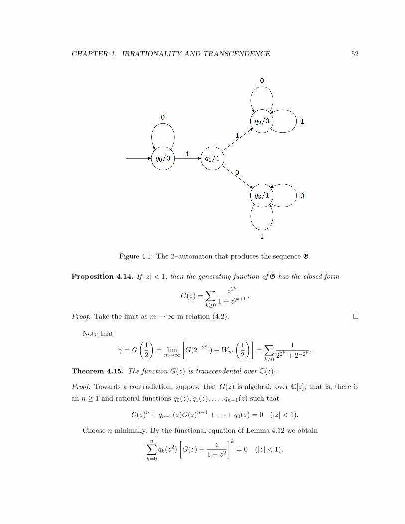
CHAPTER 4. IRRATIONALITY AND TRANSCENDENCE 52
Figure 4.1: The 2–automaton that produces the sequence G.
Proposition 4.14. If |z| < 1, then the generating function of G has the closed form
G(z) =∑k≥0
z2k
1 + z2k+1 .
Proof. Take the limit as m→∞ in relation (4.2).
Note that
γ = G
(12
)= lim
m→∞
[G(2−2m
) +Wm
(12
)]=∑k≥0
122k + 2−2k .
Theorem 4.15. The function G(z) is transcendental over C(z).
Proof. Towards a contradiction, suppose that G(z) is algebraic over C[z]; that is, there is
an n ≥ 1 and rational functions q0(z), q1(z), . . . , qn−1(z) such that
G(z)n + qn−1(z)G(z)n−1 + · · ·+ q0(z) = 0 (|z| < 1).
Choose n minimally. By the functional equation of Lemma 4.12 we obtainn∑k=0
qk(z2)[G(z)− z
1 + z2
]k= 0 (|z| < 1),

CHAPTER 4. IRRATIONALITY AND TRANSCENDENCE 53
so that for |z| < 1
P (z) : =n∑k=0
qk(z2)[(1 + z2)G(z)− z]k[1 + z2]n−k
=n∑k=0
qk(z2)[1 + z2]n−kk∑j=0
(k
j
)(1 + z2)jG(z)j(−z)k−j = 0.
Thus
Q(z) := qn(z)P (z)− (1 + z2)nqn(z2)n∑k=0
qk(z)G(z)k = 0. (4.3)
Inspection of Q(z) gives the k = n term as
qn(z)qn(z2)
n∑j=0
(n
j
)(1 + z2)jG(z)j(−z)n−j − (1 + z2)nG(z)n
.
The coefficient of Gn(x) is given when we set j = n in the preceding line, and is
qn(z)qn(z2)((
n
n
)(1 + z2)nG(z)n(−z)n−n − (1 + z2)nG(z)n
)= 0.
Hence (4.3) defines polynomials h1(z), . . . , hn−1(z) such that
Q(z) =n−1∑k=0
hk(z)G(z)k = 0.
The minimality of n implies that hk(z) = 0 for k = 0, . . . , n− 1.
Let us now determine hk(z) using the definition of Q(z) from (4.3). We have
Q(z) =n−1∑k=0
hk(z)G(z)k
=n∑k=0
k∑j=0
(k
j
)qn(z)qk(z2)(1 + z2)n−k+jG(z)j(−z)k−j
− (1 + z2)nqn(z2)qk(z)G(z)k.
From here we can read off the coefficient of G(z)m as
hm(z) =n∑
k=m
(k
m
)qk(z2)(1 + z2)n−k+m(−z)k−m − (1 + z2)nqm(z).

CHAPTER 4. IRRATIONALITY AND TRANSCENDENCE 54
Since hn−1(z) = 0, we have
n∑k=n−1
(k
n− 1
)qk(z2)(1 + z2)n−k+n−1(−z)k−(n−1) = (1 + z2)nqn−1(z).
Hence,
qn−1(z2)(1 + z2)n − nz(1 + z2)n−1 = (1 + z2)nqn−1(z),
so that we may focus on the equation
(1 + z2)qn−1(z2)− nz = (1 + z2)qn−1(z).
Write qn−1(z) = a(z)b(z) , where a(z) and b(z) are polynomials with no common factors. Sub-
stituting and clearing denominators, we obtain
(1 + z2)a(z2)b(z)− nzb(z)b(z2) = (1 + z2)a(z)b(z2). (4.4)
Using simple divisibility rules, (4.4) gives the following two conditions:
(i)b(z)G(x)
∣∣∣∣ (1 + z2)b(z2)G(x)
and (ii)b(z2)G(x)
∣∣∣∣ (1 + z2)b(z)G(x)
,
where G(x) = gcd(b(z), b(z2)). Recall that (1 + z2) = (1 + iz)(1− iz).A side note on determining properties of b(z): condition (ii) indicates the degree rela-
tionship, 2 deg b(z) ≤ 2 + deg b(z), and equation (4.4) implies that (z2 + 1) | b(z)b(z2) which
gives 2 ≤ 3 deg b(z). Together this yields a degree condition on b(z) of 1 ≤ deg b(z) ≤ 2,
since the degree must be a positive integer. In light of conditions (i) and (ii), we have
deg b(z) = 2.
Now conditions (i) and (ii) imply that either
(1 + iz) | b(z) and (1− iz)∣∣ b(z2), (4.5)
or
(1− iz) | b(z) and (1 + iz)∣∣ b(z2). (4.6)
Given the above conditions, we have two options for b(z):
condition (4.5) =⇒ b(z) = (z + 1)(z − i),
or
condition (4.6) =⇒ b(z) = (z + 1)(z + i).

CHAPTER 4. IRRATIONALITY AND TRANSCENDENCE 55
Let us assume that condition (4.5) holds and that b(z) = (z + 1)(z − i). Then (4.4)
becomes
(1 + z2)(z + 1)(z − i)a(z2)− nz(z + 1)(z − i)(z2 + 1)(z2 − i) = (1 + z2)(z2 + 1)(z2 − i)a(z).
Removing common factors, the last equation becomes
(z + 1)a(z2)− nz(z + 1)(z2 − i) = (z + i)(z2 − i)a(z). (4.7)
Equation (4.7) implies that (z+ 1) | a(z), and so (z2 + 1) | a(z2). Thus there exist k(z), l(z)
such that
a(z) = k(z)(z + 1) and a(z2) = l(z)(z2 + 1) = l(z)(z + i)(z − i).
Equation (4.7) becomes
(z + 1)l(z)(z + i)(z − i)− nz(z + 1)(z2 − i) = (z + i)(z2 − i)k(z)(z + 1),
implying that
(z + i) | nz(z + 1)(z2 − 1),
which is not possible. Hence it must be the case that b(z) 6= (z+ 1)(z− i), and so condition
(4.5) is not possible.
It must now be the case that condition (4.6) holds, that b(z) = (z + 1)(z + i). Then
(4.4) becomes
(1 + z2)(z + 1)(z + i)a(z2)− nz(z + 1)(z + i)(z2 + 1)(z2 + i) = (1 + z2)(z2 + 1)(z2 + i)a(z).
Removal of common factors yields
(z + 1)a(z2)− nz(z + 1)(z2 + i) = (z − i)(z2 + i)a(z). (4.8)
Similar to the previous case, (4.8) implies that (z + 1) | a(z), and so (z2 + 1) | a(z2). Thus
there exist k(z), l(z) such that
a(z) = k(z)(z + 1) and a(z2) = l(z)(z2 + 1) = l(z)(z + i)(z − i).
Equation (4.8) becomes
(z + 1)l(z)(z + i)(z − i)− nz(z + 1)(z2 + i) = (z − i)(z2 + i)k(z)(z + 1),
CHAPTER 4. IRRATIONALITY AND TRANSCENDENCE 56
implying that
(z + i) | nz(z + 1)(z2 + i),
which is impossible. Since one of conditions (4.5) or (4.6) must hold, we arrive at our final
contradiction, and the theorem is proved.
We proceed to show that γ is transcendental over Q, by again using Mahler’s method.
Lemma 4.12, Theorem 4.15, and Theorem 3.4 give our next theorem.
Theorem 4.16. The Gaussian Liouville number
γ = G
(12
)=∑k≥0
122k + 2−2k
is transcendental over Q.
Proof. Lemma 4.12 gives the functional equation
G(z2) =(1 + z2)G(z)− z
1 + z2,
so that, in the language of Theorem 3.4, we have
A(u) = (1 + z2)u− z and B(u) = 1 + z2,
m = 1 < 2 = d, and ai(z), bi(z) ∈ IK [z]. Since B(u) is a constant polynomial in u, we have
∆(z) := Res(A,B) = 1 + z2.
Set α = 12 . It is immediate that α = 1
2 is algebraic, 0 < |α| = 12 < min1, R (R = 1), and
∆(α2k) = ∆(2−2k
) = 1 + 2−2k+1 6= 0 (k ≥ 0).
Since G(z) is not algebraic over C[z] (as supplied by Theorem 4.15), applying Theorem 3.4,
we have that γ is transcendental over Q.
4.2.3 Transcendence related to character–like functions
A character–like function f associated to p is a completely multiplicative function from Nto −1, 1 defined by f1 = 1, fp = ±1 (your choice), and fkp+i = fi. As an example, the
completely multiplicative function defined by
fn =
±1 if n = p(np
)if p - n,

CHAPTER 4. IRRATIONALITY AND TRANSCENDENCE 57
where(np
)is the Legendre symbol modulo p, is a character–like function.
If we let f be a character–like function associated to p, then for F (z) =∑
n≥1 fnzn
the generating function of the sequence F := (fn) we have a lemma similar to the previous
subsections.
Lemma 4.17. The generating function F (z) of the sequence F satisfies the functional equa-
tion
F (z) = fpF (zp) +Φ(z)
1− zp,
where Φ(z) =∑p−1
i=1 fizi.
Proof. We have
F (z) =∑k≥0
p−1∑i=1
fpk+izpk+i +
∑k≥1
fpkzpk
=p−1∑i=1
fizi∑k≥0
zpk + fp∑k≥1
fkzpk
=∑p−1
i=1 fizi
1− zp+ fpF (zp).
Theorem 4.18. The function F (z) is transcendental.
Proof. Note that since z = 1 is a root of 1 − zp and Φ(1) =∑p−1
i=1 (i/p) = 0, the rational
function Φ(z)1−zp may be written as the ratio of two polynomials, both of which have degree
strictly less than p. Hence an application of Theorem 3.13 gives the result.
Using the functional equation, we yield
F (zp) = fpF (z)− fpΦ(z)
1− zp.
We can build a series for the number as before. The functional equation gives
F (zpm
) = fpF (zpm−1
)− fpΦ(zp
m−1)
1− zpm
= f2pF (zp
m−2)− f2
p
Φ(zpm−2
)1− zpm−1 − fp
Φ(zpm−1
)1− zpm
= fmp F (z)−m∑k=1
fkpΦ(zp
m−k)
1− zpm−k+1 ,

CHAPTER 4. IRRATIONALITY AND TRANSCENDENCE 58
which when rearranged leads to
F (z) = fmp F (zpm
) +m∑k=1
fm−kp
Φ(zpm−k
)1− zpm−k+1 .
We change the index and set
Vm(z) :=m−1∑k=0
fkpΦ(zp
k)
1− zpk+1
to give
F (z) = fmp F (zpm
) + Vm(z).
Proposition 4.19. The generating function F (z) has the closed form
F (z) =∑k≥0
fkpΦ(zp
k)
1− zpk+1 .
Proof. Take the limit as m→∞ in the equation F (z) = fmp F (zpm
) + Vm(z).
At z = 1/2 we have
F
(12
)= lim
m→∞
[fmp F (2−p
m) + Vm
(12
)]=∑k≥0
fkpΦ(2−pk)
1− 2−pk+1 .
Theorem 4.20. For each odd prime p, the number ϕp := F(
12
)is transcendental.
Proof. Lemma 4.17 gives
F (zp) =fp(1− zp)F (z)− fpΦ(z)
1− zp,
where Φ(z) =∑p−1
i=1 fizi. Similar to the specific case of the previous section, using the
language of Mahler’s Theorem, we have
A(u) = fp(1− zp)u− fpΦ(z) and B(u) = 1− zp,
m = 1 < p = d, and ai(z), bi(z) ∈ IC[z]. Again, B(u) is a constant polynomial in u, so that
∆(z) := Res(A,B) = 1− zp.
Set α = 12 ; α = 1
2 is algebraic, 0 < |α| = 12 < min1, R (R = 1), and
∆(αpk) = ∆(2−p
k) = 1− 2−p
k+1 6= 0 (k ≥ 0).
Theorem 4.18 gives that F (z) is not algebraic over C[z] and we may apply Theorem 3.4 to
give the desired result.

CHAPTER 4. IRRATIONALITY AND TRANSCENDENCE 59
Remark 4.21. Mahler’s Theorem tells us that the values of the power series G(z) and F (z)
are transcendental for any algebraic value of z within their radii of convergence. The special
value of z = 12 is focused on only for its relation to the sequences G and F.
Remark 4.22. There is a very powerful theorem of Adamczewski and Bugeaud [1] which
states that if β =∑
n a(n)b−n is a base b automatic irrational, then β is transcendental.
Their proof uses the Schmidt Subspace Theorem, and avoids Mahler theory. Mahler’s theory
still yields a more complete result, as it gives transcendence of a series at not just the values1b for b ≥ 2, but for all algebraic values in the region of convergence. Indeed, it is not known
whether a Mahler–theoretic proof of Adamczewski and Bugeaud’s result is possible.

Chapter 5
(Non)Automaticity
5.1 Automaticity
The general theory of automaticity is not a well–known area to many number theorists.
This section contains background results for those who are not well acquainted with this
theory. Unless otherwise noted, the definitions, theorems, and proofs in this section have
been taken from Allouche and Shallit [6].
Definition 5.1. A k–deterministic finite automaton with output (k-DFAO) is defined to be
a 6–tuple
M = (Q,Σk, δ, q0,∆, τ)
where Q is a finite set of states, Σk = 0, 1, . . . , k − 1 is the finite input alphabet, δ :
Q×Σk → Q is the transition function, q0 ∈ Q is the initial state, ∆ is the output alphabet,
and τ : Q→ ∆ is the output function.
Definition 5.2. We say that the sequence (a(n))n≥0 over a finite alphabet ∆ is k–automatic
if there exists a k–DFAO M = (Q,Σk, δ, q0,∆, τ) such that a(n) = τ(δ(q0, w)) for all n ≥ 0
and all w with [w]k = n.
While the definition of a k–DFAO has a computational appeal, from a theoretical point
of view, for the types of results we are interested in, the setting of Definition 5.2 is more
tractable.
Theorem 5.3. The sequence (a(n))n≥0 is k–automatic if and only if there exists a k–DFAO
M such that a(n) = τ(δ(q0, (n)k)) for all n ≥ 0. Moreover, we may choose M such that
60
CHAPTER 5. (NON)AUTOMATICITY 61
δ(q0, 0) = q0.
Proof. The first direction is clear from the definition. For the other, let M = (Q,Σk, δ, q0,∆,
τ) and define M ′ = (Q′,Σk, δ′, q′0,∆, τ
′) by
Q′ = Q ∪ q′0,
δ′(q, b) = δ(q, b) for all q ∈ Q, b ∈ Σk,
δ(q′0, b) =
δ(q0, q) if a 6= 0,
q′0 if a = 0,
τ ′(q′0) = τ(q0),
t′(q) = τ(q) for all q ∈ Q.
For n 6= 0, we have
δ′(q′0, 0i(n)k) = δ′(q0, (n)k) = δ(q0, (n)k).
Hence
τ ′(δ′(q′0, 0i(n)k)) = τ(δ(q0, (n)k)).
If we allow the k–DFAO to take the base k expansion of an integer n as input, starting
with the least significant digit, we have the following theorem (see Theorem 5.2.3 of [6]).
Theorem 5.4. The following three conditions are equivalent:
(i) (a(n))n≥0 is a k–automatic sequence.
(ii) There exists a k–DFAO M = (Q,Σk, δ, q0,∆, τ) such that a(n) = τ(δ(q0, wR)) for all
n ≥ 0 and all finite words w from the alphabet Σk such that [w]k = n.
(iii) There exists a k–DFAO M ′ = (Q′,Σk, δ′, q′0,∆, τ
′) such that a(n) = τ(δ(q0, (n)Rk )) for
all n ≥ 0.
For those of us are not comfortable with the k–DFAO terminology, the above definition
of a k–automatic sequence can be confusing. Fortunately, there is an equivalent way to view
this concept which, in our opinion, is more intuitive.
Definition 5.5. Let a = (a(n))n≥1 be a sequence with values from a finite set. Define the
k–kernel of a as the set
Kk(a) = (a(kln+ r))n≥0 : l ≥ 0 and 0 ≤ r < kl.

CHAPTER 5. (NON)AUTOMATICITY 62
Theorem 5.6. Let k ≥ 2. The sequence a = (a(n))n≥0 is k–automatic if and only if Kk(a)
is finite.
Proof. Let k ≥ 2. Suppose that a = (a(n))n≥0 is k–automatic sequence. Then it follows
from Theorem 5.4 that there is a k–DFAO M = (Q,Σk, δ, q0,∆, τ) such that
a(n) = τ(δ(q0, (n)Rk 0t)) ∀t ≥ 0.
Now let q = δ(q0, wR) where |w| = i and [w]k = j. Since
(kin+ j)k = (n)kw
expect possibly when n = 0, it follows that, for n > 0, we have
δ(q0, (kinj)Rk ) = δ(δ(q0, wR), (n)Rk ) = δ(q, (n)Rk ).
In the case when n = 0 we have
(kin+ j)k = (j)k,
and w = 0t(j)k for some t ≥ 0. Then
δ(q0, (kinj)Rk ) = δ(q0, (j)Rk ) = δ(q0, (j)Rk 0t) = δ(q0, wR) = q = δ(q, (0)Rk ).
It follows that the subsequence (a(kin+ j))n≥0 is generated by the k–DFAO (Q,Σk, δ, q,
∆, τ). Since there are only finitely many choices for q, the finiteness of Kk(a) follows.
Now suppose that Kk(a) is finite. Then the set of finite words on Σk is partitioned into
a finite number of disjoint equivalence classes under the equivalence relation
w ≡ x if and only if a(k|w|n+ [w]k) = a(k|x|n+ [x]k)
for all n ≥ 0.
We make a k–DFAO as follows:
Q = [x] : x is a finite word on Σk, δ([x], b) = [bx], τ([w]) = a([w]k), q0 = [ε],
where [x] is the equivalence class containing x. We need to see that this definition is
meaningful, that is, if [x] = [w], then δ([x], b) = δ([w], d) and τ([x]) = τ([w]). For the first,
we need [bx] = [bw]. Now if [x] = [w] then
a(k|w|n+ [w]k) = a(k|x|n+ [x]k)

CHAPTER 5. (NON)AUTOMATICITY 63
for all n ≥ 0. Setting n = km+ b it follows that
a(k|aw|m+ [aw]k) = a(k|ax|m+ [ax]k)
for all m ≥ 0.
For the second assertion we need to see that if
a(k|w|n+ [w]k) = a(k|x|n+ [x]k)
then
a([w]k) = a([x]k).
To do this, set n = 0. We now claim that τ(δ(q0, wR)) = a([w]k) for all finite words w on Σk.
By induction on |w| we have δ(q0, wR) = [w]. By the definition of τ the result follows.
Connecting automaticity to transcendence, we have the following beautiful and crucial
theorem of Christol et al. which is essential to the results of this chapter. The proof given
here is our translation from the original French [23].
Theorem 5.7 (Christol et al. [23]). Let Σ be a finite nonempty alphabet, t = (tn) ∈ ΣN ,
and p be a prime number. Then the sequence t is p–automatic if and only if there exists a
field K of characteristic p and an injection α : Σ→ K such that α(t) = (α(tn)) is algebraic
over K(X).
Proof. Suppose that t ∈ ΣN is a p–automatic sequence. Also, let K be a finite field of
characteristic p having at least as many elements as Σ. Thus Σ can be embedded in K.
After renaming the elements of Σ, we may consider t ∈ KN . We show that t is algebraic
over K(X).
Denote the number of elements of K by q := ps.
For r ∈ [q], we consider the application Ar : K[[X]]→ K[[X]] defined by
Ar
(∑n
vnXn
)=∑n
vqn+rXn.
Let N be the semigroup generated by the identity and the Ar under composition. For all
v =∑
n vnXn ∈ K[[X]] we associate its orbit
N (v) = A(v) : A ∈ N.

CHAPTER 5. (NON)AUTOMATICITY 64
By Theorem 5.6, we know that N (v) is finite if and only if v is q–automatic, that is to say
p–automatic (see [41, Proposition 3.3, p. 107]). Thus N (t) is finite.
Let E be the vector space over K(X) generated by N (t) and F the vector space over
K(X) generated by the gq, where g ∈ N (t). We show initially that E = F . Indeed, if
g1, g2, . . . , gN are a basis of E, then for all g ∈ E we have
g =N∑k=1
ckgk
thus
gq =N∑k=1
cqkgqk
which shows that gq1, gq2, . . . , g
qN is a system of generators of F . Thus
dimF ≤ dimE ≤ cardN (t).
In addition, for all g ∈ N (t), we have
g =q−1∑r=0
Xr(Ar(g))q.
However (Ar(g))q ∈ (N (t))q ⊂ F, thus E ⊂ F , so that the preceding inequality gives E = F .
Now let G be the vector space over K(X) generated by products of the type∏g∈N (t)
gβ(g),
where β : N (t) → N is not identically zero. Then t ∈ G, where G is a ring with tG ⊂ G.
However, a classical result [69, p. 2] gives the implication
dimG <∞ ⇒ t is algebraic
and the degree of t is bounded by dimG. Thus to establish that t is algebraic is suffices to
show that G has finite dimension.
Let g ∈ N (t). Then since E = F , we have that gq is a linear combination of h ∈ N (t)
with coefficients in K(X). Consequently, G is generated by the products∏g∈N (t)
gβ(g) where β(g) < q.

CHAPTER 5. (NON)AUTOMATICITY 65
It follows that
dimG ≤ qcardN (t) − 1.
This gives the first implication of the theorem.
For the other direction let K be a finite field of characteristic p of q = ps elements,
f = (fn) a sequence algebraic overK(X), α an injection of Σ intoK, and t = (tn) = (α−1fn).
We show below that t is q–automatic, and hence by [41] t is p–automatic, which gives that
f is q–automatic.
We use the same notations as above. As we have already seen, it suffices to show that
N (f) is finite.
Since f is algebraic over K(X), the vector space generated by the fn (n ∈ N) has finite
dimension over K(X), and thus there exist a0, . . . , ak in K[X] not all zero such that
k∑i=0
aifqi
= 0.
Let j be the least integer for which there is a relation of the preceding type with aj 6= 0.
We show that j = 0. Indeed, since
aj =q−1∑r=0
Xr(Ar(aj))q,
there exists an r with Ar(aj) 6= 0.
From the relation∑k
i=j aifqi
= 0, we deduce that∑k
i=j Ar(aifqi
) = 0, and taking into
account that for g and h in K(X) we have Ar(gqh) = gAr(h), and supposing j 6= 0, we have
k∑i=j
Ar(ai)f qi−1
= 0
which is a relation of the preceding type where the coefficient of f qj−1
is different from 0,
which is in contradiction to the hypothesis made on j.
Thus we have the relationk∑i=0
aifqi
= 0 with a0 6= 0.
Writing g = f/a0, we have
g =k∑i=1
bigqi
where bi = −aiaqi−2
0 ∈ K[X].
CHAPTER 5. (NON)AUTOMATICITY 66
Let N = sup(deg a0, supi=1,...,k deg bi), and let H be the set of h ∈ K[[X]] of the form
h =k∑i=0
cigqi, ci ∈ K[X], deg ci ≤ N,
H is a finite set, and f = a0g belongs to h. It suffices to show that H is stable under
applications Ar.
However, if h belongs to H, we have
Ar(h) = Ar
(c0g +
k∑i=1
cigqi
)= Ar
(k∑i=1
(c0bi + ci)gqi
)=
k∑i=1
Ar(c0bi + ci)gqi−1.
Since deg(c0bi + ci) ≤ 2N , we have that degAr(c0bi + ci) ≤ 2N/q ≤ N and consequently
Ar(h) belongs to H, which finishes the proof of the theorem.
For the remainder of this chapter, we rely heavily on the following corollary of the
previous theorem of Christol et al.
Corollary 5.8. Let Fp be a finite field and (a(n))n≥0 be a sequence with values in Fp. Then,
the sequence (a(n))n≥0 is p–automatic if and only if the formal power series∑
n≥0 a(n)Xn
is algebraic over Fp(X).
5.2 (Non)Automaticity of arithmetic functions
In Banks, Luca, and Shparlinski [8], it is shown that the series∑n≥1
f(n)Xn ∈ Z[[X]] (5.1)
is not a rational function with coefficients in Z when f is taken to be any of the number–
theoretic functions
ϕ, τ, σ, λ, µ, ω,Ω, p, or ρ. (5.2)
Here ϕ(n), the Euler totient function, is the number of positive integers m ≤ n with
gcd(m,n) = 1, τ(n) is the number of positive integer divisors of n, σ(n) is the sum of
those divisors, ω(n) is the number of distinct prime divisors of n, Ω(n) is the number of
total prime divisors of n, λ(n) = (−1)Ω(n) is Liouville’s function, µ(n) is the Mobius function

CHAPTER 5. (NON)AUTOMATICITY 67
defined by
µ(n) =
1 if n = 1,
0 if k2 | n for some k ≥ 2,
(−1)ω(n) if k2 - n for all k ≥ 2,
p(n) is the n–th prime number, and ρ(n) = 2ω(n) counts the number of square–free positive
divisors of n.
In the course of this investigation we give, or give reference to, results showing that the
series∑
n≥1 f(n)Xn ∈ Z[[X]] is transcendental over Z(X), for all of the functions f in (5.2).
In most cases, the stronger result of transcendence of the series in Fp[[X]] over Fp(X) is
shown. To get at these stronger results we rely upon Corollary 5.8.
Since any algebraic relation in Z(X) is an algebraic relation in Fp(X), we have
Lemma 5.9. Let p be a prime. If a series F (X) ∈ Z[[X]] and its termwise reduction
F (X) ∈ Fp[[X]] is transcendental over Fp(X), then F (X) ∈ Z[[X]] is transcendental over
Z(X).
Between Allouche [3] and Yazdani [98] we have that for any prime p, the series (5.1) is
transcendental over Fp(X) (and so over Z(X) by the lemma) for f = ϕ, τk, σk, and µ. Recall
that
τk(n) := #(a1, a2, . . . , ak) : a1a2 · · · ak = n, ai ∈ N for i = 1, . . . , k
and σk(n) is the sum of the kth powers of the divisors of n (note that τ2(n) = τ(n) and
σ1(n) = σ(n)). In the previous chapter we showed that the series (5.1) is transcendental
over Z(X) for any completely multiplicative function f : N→ −1, 1 that is not identically
1; this includes f = λ. We summarize in the following two theorems.
Theorem 5.10 (Allouche [3], Yazdani [98]). The series∑
n≥1 f(n)Xn is transcendental
over Fp(X) for f = (g mod v) with g = ϕ, τm, σm, and µ where m ≥ 1 and v ≥ 2.
Theorem 5.11. The series∑
n≥1 f(n)Xn is transcendental over Z(X) for any nontrivial
completely multiplicative function taking values in −1, 1 (this includes f = λ).
In Section 5.3, answering a question of Yazdani [98], we give the main result of this
chapter is an improvement of Theorem 5.11.
Theorem 5.12. Liouville’s function λ is not k–automatic for any k ≥ 2, and hence∑n≥1 λ(n)Xn ∈ Fp[[X]] is transcendental over Fp(X) for all p > 2.

CHAPTER 5. (NON)AUTOMATICITY 68
We can use Theorem 5.12 to prove a similar result for Ω(n). We also use the following
direct consequence of the definition of automaticity.
Remark 5.13. Let t : N → Y and Φ : Y → Z be mappings. If (t(n))n≥1 is k–automatic
for some k ≥ 2, then (Φ(t(n)))n≥1 is also k–automatic.
Note that the values of Ω(n) viewed modulo 2 satisfy
(Ω(n) mod 2) =1− λ(n)
2.
Using this relationship, Remark 5.13 and Theorem 5.12 give the following corollary.
Corollary 5.14. The function (Ω(n) mod 2) is not 2–automatic. Furthermore, the series∑n≥1 Ω(n)Xn is transcendental over both F2(X), and Z(X).
Ritchie [86] showed that the characteristic function of the squares is not 2–automatic.
Combining this result with Remark 5.13 gives a nice corollary regarding τ(n).
Corollary 5.15. The sequence (τ(n) mod 2) is not 2–automatic. Hence∑
n≥1 τ(n)Xn is
transcendental over both F2(X) and Z(X).
Proof. The function τ(n) taken modulo 2 is the characteristic function of the squares.
One of the nicest results in this area is that of Hartmanis and Shank on the non–
automaticity of the characteristic function of the primes.
Theorem 5.16 (Hartmanis and Shank [56]). The characteristic function of the primes, χP ,
is not k–automatic for any k ≥ 2.
In Section 5.3, we give new (short and analytic) proofs of Theorem 5.16, as well as its
extension to all prime powers, and Corollary 5.14. Many other functions, such as ρ, are
also considered in this section. In Section 5.4, we also address unbounded multiplicative
functions using the generalization of k–automatic sequences to k–regular sequences.
The differences in transcendence over Z(X) and Fp(X) are quite pronounced. Theo-
rem 5.11 gives transcendence over Z(X) of a very large class of functions, many of which
are k–automatic for some k ≥ 2 and hence their reduction over some finite field is alge-
braic. For those (f(n))n≥0 that are automatic, one can use the theory of Mahler [73, 83]
to give transcendence results regarding the values of the series∑
n≥1 f(n)Xn ∈ Z[[X]]. For
non–automatic sequences almost no progress has been made. For example, the following
conjecture is still open.

CHAPTER 5. (NON)AUTOMATICITY 69
Conjecture 5.17. Let f : N → −1, 1 be a completely multiplicative function for which
f(p) = −1 for at least one prime p. Then the number∑
n≥1 f(n)2−n is transcendental over
Q.
Remark 5.18. As some support for this conjecture, we may focus on those sequences
here which are automatic. By Theorem 4.8, all of the numbers described in Conjecture
5.17 are irrational. A theorem of Adamczewski and Bugeaud [1], implies that if (f(n))n≥1
from Conjecture 5.17 is k–automatic for some k ≥ 2, then the number∑
n≥1 f(n)2−n is
transcendental over Q.
5.3 Dirichlet series and (non)automaticity
We rely heavily on a theorem of Allouche, Mendes France, and Peyiere [5], and also on the
details of its proof. Before preceding to this theorem, we need some additional properties
of k–automatic sequences (see [5] for details).
Let k ≥ 2 and (u(n))n≥1 be a k–automatic sequence with values in C. Then there exist
an integer t ≥ 1 and a sequence (Un)n≥1 with values in Ct (which we denote as a column
vector) as well as k matrices of size t× t denoted by A1, A2, . . . , Ak, with the property that
each row of each Ai has exactly one entry equal to 1 and the rest equal to 0 (he fact that these
are ones and zeros comes from the finiteness of the k–kernel of (u(n))n≥1), such that the
first component of the vector (Un)n≥1 is the sequence (u(n))n≥1 and for each i = 1, 2, . . . , k,
and for all n ≥ 1, we have
Ukn+i = AiUn.
Theorem 5.19 (Allouche, Mendes France, and Peyiere, [5]). Let k ≥ 2 be an integer
and let (u(n))n≥0 be a k–automatic sequence with values in C. Then the Dirichlet series∑n≥1 u(n)n−s is the first component of a Dirichlet vector (i.e., a vector of Dirichlet series)
G(s), where G has an analytic continuation to a meromorphic function on the whole complex
plane, whose poles (if any) are located on a finite number of left semi–lattices.
Proof. We follow the proof in [5], but with some slight modifications. Define a Dirichlet
vector G(s) for <s > 1 by
G(s) =∑n≥1
Unns.

CHAPTER 5. (NON)AUTOMATICITY 70
Since Ukn+j = AjUn, we have
G(s) =k−1∑j=1
∑n≥1
AjUn(kn+ j)s
+∑n≥1
AkUn(kn)s
.
Writing I as the t× t identity matrix, we have
(I − k−sAk)G(s) =k−1∑j=1
∑n≥1
AjUn(kn+ j)s
=k∑j=1
Aj∑n≥1
k−sn−sUn
(1 +
j
kn
)−s
=k∑j=1
Aj∑m≥0
(s+m− 1
m
)(−j)mG(s+m)
ks+m,
and so
(I − k−s(A0 +A1 + · · ·+Ak))G(s) =k∑j=1
Aj∑m≥1
(s+m− 1
m
)(−j)mG(s+m)
ds+m. (5.3)
Denote A := k−1∑k
j=1Aj and byM(X) the transpose of the comatrix of (A−XI), so that
M(X)(A−XI) = (A−XI)M(X) = det(A−XI)I.
Multiplying (5.3) by M(ks−1), we have
det(A− ks−1I)G(s) = −M(ks−1)k∑j=1
Aj∑m≥1
(s+m− 1
m
)(−j)mG(s+m)
ks+m. (5.4)
For a given s ∈ C, the function G(s + m) is bounded for m large enough. Thus the right–
hand side of (5.4) converges for <s > 0, so that this gives a meromorphic continuation
to <s ∈ (0, 1] with possible poles at points s for which ks−1 is an eigenvalue of A. If
<s ∈ (−1, 0], the right-hand side of (5.4) converges with the possible exception of those
s for which ks is an eigenvalue of A. This gives a meromorphic continuation of G to this
region with possible poles at points s for which either ks−1 or ks is an eigenvalue of A.
Continuing this process gives an analytic continuation of G to a meromorphic function on
all of C with possible poles at points
s =logαlog k
+2πi
log km− l + 1,
where α is an eigenvalue ofA, m ∈ Z, l ∈ N and log is a branch of the complex logarithm.

CHAPTER 5. (NON)AUTOMATICITY 71
Remark 5.20. A one–dimensional version of Theorem 5.19 for the Thue–Morse Dirichlet
series was given by Allouche and Cohen [4]. It is also worth noting that such an infinite
functional equation is classical for ζ(s), the Riemann zeta function, though it is much less
deep than the usual functional equation for ζ(s).
The beauty of the above proof is in the details, which is why we have chosen to reproduce
it here. Note that the possible poles are explicitly given, as is the meromorphic continuation.
This leads to a few nice classifications regarding Dirichlet series.
Proposition 5.21. If the Dirichlet series∑
n≥1 f(n)n−s is not meromorphically continuable
to the whole complex plane then (f(n))n≥1 is not k–automatic for any k ≥ 2.
Our first application of this is a new proof of the well–known result of Hartmanis and
Shank about the non–automaticity of the characteristic function of the primes.
Proof of Theorem 5.16. In 1920, Landau and Walfisz [68] proved that the Dirichlet series
P (s) :=∑
p p−s is not continuable past the line <s = 0. This is a consequence of the identity
P (s) =∑n≥1
µ(n)n
log ζ(ns).
Since ζ(s) has a pole at s = 1, this relationship shows that s = 1/n is a singular point for
all square–free positive integers n. This sequence limits to s = 0. Indeed, all points on the
line <s = 0 are limit points of the poles of P (s) (see [92, pages 215–216] for details) so that
the line <s = 0 is a natural boundary for P (s).
Minsky and Papert [77] were the first to address this question, showing that the char-
acteristic function of the primes is not 2–automatic. Hartmanis and Shank [56] gave the
complete result. Similar to our proof of Theorem 5.16, denoting by
χΠ(n) :=
1 if n is a prime power
0 otherwise,
and using the relationship ∑n≥1
χΠ(n)ns
=∑k≥1
∑n≥1
µ(n)n
log ζ(kns),
we have the corresponding result for prime powers.

CHAPTER 5. (NON)AUTOMATICITY 72
Proposition 5.22. The sequence (χΠ(n))n≥1 is not k–automatic for any k ≥ 2.
Proposition 5.23. Define the function r(n) by 2 · r(n) = ρ(n). The sequence (r(n) mod 2)
is not 2–automatic; hence∑
n≥1 ρ(n)Xn is transcendental over Z(X).
Proof. This follows from the the fact that (r(n) mod 2) = χΠ(n) and an application of
Proposition 5.22.
As alluded to, the proof of Theorem 5.19 reveals much in the way of details. Indeed, due
to the explicit determination of the poles, we can can provide a very useful classification,
but first, a definition.
Definition 5.24. Denote by R(a, b;T ) the rectangular subset of C defined by <s ∈ [a, b]
and =s ∈ [0, T ], by N∞(F (s), R(a, b;T )) the number of poles of F (s) in R(a, b;T ), and by
N0(F (s), R(a, b;T )) the number of zeros of F (s) in R(a, b;T ).
Proposition 5.25. Let k ≥ 2, (f(n))n≥1 be a k–automatic sequence and let F (s) denote
the Dirichlet series with coefficients (f(n))n≥1. If a, b ∈ R with a < b, then
N∞(F (s), R(a, b;T )) = O(T ).
Hence, if G(s) =∑
n≥1 g(n)n−s (<s > α for some α ∈ R) is meromorphically continu-
able to a region containing a rectangle R(a, b, T ) for which
limT→∞
1TN∞(F (s), R(a, b, T )) =∞,
then (g(n))n≥1 is not k–automatic for any k ≥ 2.
Proof. This is a direct consequence of the poles of F being located on a finite number of
left semi–lattices.
From here on, we make systematic use of a classical result by von Mangoldt.
Theorem 5.26 (von Mangoldt [94]). The number of zeros of the function ζ(s) in the
rectangle R(0, 1;T ) is N0(ζ(s), R(0, 1;T )) T log T .
As a consequence of von Mangoldt’s theorem, we have a new proof of the following
theorem of Allouche [2] (see also [3]).

CHAPTER 5. (NON)AUTOMATICITY 73
Theorem 5.27 (Allouche [2]). The sequence (µ(n))n≥1 is not k–automatic for any k ≥ 2.
Hence the series∑
n≥1 µ(n)Xn is transcendental over both Fp(X), for all primes p, and
Z(X).
Proof. From the relationship ∑n≥1
µ(n)ns
=1ζ(s)
(<s > 1),
for the result, we need only show that
limT→∞
1TN∞
(1ζ(s)
, R(0, 1 : T ))
=∞.
This is given by Theorem 5.26. Application of Proposition 5.25 proves the theorem.
It is note–worthy that our proof for µ(n), and the proof for |µ(n)| below, does not use
Cobham’s theorem [26] on rational densities: if a sequence is k–automatic for some k ≥ 2,
then the density, provided it exists, of the occurrence of any value of that sequence is rational.
In a similar fashion to the above results, using the extention to Dirichlet L–functions of
von Mangoldt’s theorem, we may generalize this result further.
Lemma 5.28. We have N0(L(s, χ), R(0, 1;T )) T log T .
Corollary 5.29. Let χ be a Dirichlet character. Then (µ(n)χ(n))n≥1 is not k–automatic
for any k ≥ 2.
Proof. This follows directly from the fact that the sequence (µ(n)χ(n))n≥1 is the sequence
of coefficients of the series 1L(s,χ) . Application of Lemma 5.28 and Proposition 5.25 gives
the desired result.
The proof of Theorem 5.12 rests on substantially more than the previous results of this
investigation; it requires both the Prime Number Theorem in the form below as well as a
very deep result of Selberg.
Theorem 5.30 (Hadamard [53], de la Vallee Poussin [32]). The Riemann zeta function has
no zeros on the line <s = 1.
Theorem 5.31 (Selberg [89]). A positive proportion of the zeros of the Riemann zeta func-
tion lie on the line <s = 12 .
CHAPTER 5. (NON)AUTOMATICITY 74
Proof of Theorem 5.12. We use the identity
L(s) :=∑n≥1
λ(n)ns
=ζ(2s)ζ(s)
(<s > 1).
Using this identity, the poles of L(s) are precisely the zeros of ζ(s) that are not cancelled by
the zeros of ζ(2s) as well as the pole of ζ(2s) at s = 12 . Selberg’s theorem gives a positive
proportion of zeros of ζ(s) on the critical line and the Prime Number Theorem tells us that
there are no zeros on the line <s = 1. By Theorem 5.26, we have
N∞
(ζ(2s)ζ(s)
, R
(12,12
;T)) T log T.
Application of Proposition 5.25 gives the result.
Invoking a stronger form of Selberg’s theorem, we may include many more number–
theoretic functions in our investigation.
Theorem 5.32 (Conrey [27]). More than two–fifths of the zeros of the Riemann zeta func-
tion lie on the critical line.
Conrey’s theorem gives the following corollary.
Corollary 5.33. Less than three–tenths of the zeros of the Riemann zeta function lie on
any line <s = α when α 6= 12 .
Proof. Recall that if ζ(s) = 0, then by the functional equation ζ(1− s) = 0. The corollary
then follows from the elementary observation that 2 · 310 + 2
5 = 1.
Recall that for m ≥ 2
qm(n) =
0 if pm | n for any prime p
1 otherwise.
Hence q2(n) = |µ(n)|.
Theorem 5.34. For k ≥ 2, the functions qm(n) (m ≥ 2) are not k–automatic, and hence
for each m ≥ 2 the series∑
n≥1 qm(n)Xn is transcendental over both Fp(X), for all primes
p, and Z(X).

CHAPTER 5. (NON)AUTOMATICITY 75
Proof. Note the identities for <s > 1:∑n≥1
qm(n)ns
=ζ(s)ζ(ms)
(m ≥ 2).
Our result relies on ζ(s)/ζ(mz) for each m ≥ 2 having more than O(T ) poles in some
rectangle. Corollary 5.33 gives
N∞
(ζ(s)ζ(ms)
, R
(1
2m,
12m
;T)) T log T.
Application of Proposition 5.25 finishes the proof.
Note that the result for |µ(n)| is already given by that of µ(n) by simply defining Φ to
be the absolute value function and applying Remark 5.13.
5.4 Dirichlet series and (non)regularity
We take the following definition from [6].
Definition 5.35. We say that a sequence S := (s(n))n≥0 taking values in a Z–module R
is a k–regular sequence, or just k–regular, provided there exist a finite number of sequences
over R, (s1(n))n≥0, . . . , (ss(n))n≥0, with the property that every sequence in the k–kernel
of S is a Z–linear combination of the si.
Compared to the finiteness of the k–kernel in the case of a k–automatic sequence, the above
definition tells us that the sequence S is k–regular provided the k–kernel of S is finitely
generated.
Using this definition, let k ≥ 2 and (v(n))n≥1 be a k–regular sequence with values in
C. Then similar to the automatic case, there exist an integer t ≥ 1 and a sequence (Vn)n≥1
with values in Ct (which we denote as a column vector) as well as k matrices of size t × tdenoted by B1, B2, . . . , Bk with integer entries (no longer just 1s and 0s as in the automatic
case), such that the first component of the vector (Vn)n≥1 is the sequence (v(n))n≥1 and for
each i = 1, 2, . . . , k, and for all n ≥ 1, we have
Vkn+i = BiVn.
These properties give the analogue of Theorem 5.19 to k–regular sequences. This result is
alluded to in [5, Remark 4].
CHAPTER 5. (NON)AUTOMATICITY 76
Theorem 5.36. Let k ≥ 2 be an integer and let (v(n))n≥0 be a k–regular sequence with
values in C. Then the Dirichlet series∑
n≥1 v(n)n−s is the first component of a Dirichlet
vector (i.e., a vector of Dirichlet series) G(s), where G has an analytic continuation to a
meromorphic function on the whole complex plane, whose poles, if any, are located on a
finite number of left semi–lattices.
The proof of this theorem is exactly that of Theorem 5.19 with Vi and Bi substituted
for Ui and Ai, respectively, for each i.
We now have the same useful corollaries that we had for k–automatic sequences.
Corollary 5.37. Let k ≥ 2. The following properties hold:
(i) If the Dirichlet series∑
n≥1 f(n)n−s is not meromorphically continuable to the whole
complex plane then (f(n))n≥1 is not k–regular.
(ii) If G(s) =∑
n≥1 g(n)n−s (<s > α for some α ∈ R) is meromorphically continuable to
a region containing a rectangle R(a, b, T ) for which
limT→∞
1TN∞(G(s), R(a, b, T )) =∞,
then (g(n))n≥1 is not k–regular.
Theorem 5.38. The function ϕ(n) is not k–regular for any k ≥ 2.
Proof. From the relationship∑n≥1
ϕ(n)ns
=ζ(s− 1)ζ(s)
(<s > 2),
and the lack of zeros of ζ(s − 1) in the region 0 ≤ <s ≤ 1 as given by the Prime Number
Theorem, we need only show that
limT→∞
1TN∞
(1ζ(s)
, R(0, 1 : T ))
=∞.
This is given by Theorem 5.26. Application of the Corollary 5.37 proves the theorem.
Theorem 5.39. For k ≥ 2, the functions ρ(n), τ(n2) and τ2(n) are not k–regular.
CHAPTER 5. (NON)AUTOMATICITY 77
Proof. Note the identities for <s > 1:∑n≥1
ρ(n)ns
=ζ2(s)ζ(2s)
,∑n≥1
τ(n2)ns
=ζ3(s)ζ(2s)
,∑n≥1
τ2(n)ns
=ζ4(s)ζ(2s)
.
Our result relies on ζ(s)/ζ(2z) having more than O(T ) poles in some rectangle. This follows
directly from the proof of Theorem 5.34.
Theorem 5.40. The functions ω(n) and Ω(n) are not k–regular for any k ≥ 2.
Proof. This follows from our proof of Theorem 5.16 and the identities∑n≥1
ω(n)ns
= ζ(s)∑k≥1
µ(k)k
log ζ(ks), and∑n≥1
Ω(n)ns
= ζ(s)∑k≥1
ϕ(k)k
log ζ(ks)
and the added stipulation that there are no zeros of ζ(s) on the line <s = 0. This is provided
for by the Prime Number Theorem and the symmetry of zeros of the Riemann zeta function
about the critical line as given by the functional equation for ζ(s).
Some of these results can be found from another direction using our knowledge of their
non–automaticity and the following theorem (see Chapter 16 of [6] for details).
Theorem 5.41 (Allouche and Shallit [6]). If the integer sequence (f(n))n≥0 is k–regular,
then for all integers m ≥ 1, the sequence (f(n) mod m)n≥0 is k–automatic.
Thus if there exists an m ≥ 1 for which (f(n) mod m)n≥0 is not k–automatic, then
(f(n))n≥0 is not k–regular. Hence the results of the previous sections give non–regularity
results for each of ω, Ω, τ , and ρ. It is also worth noting that a sequence is k-regular and
takes on only finitely many values if and only if it is k–automatic [6]. This provides a nice
relationship for non–regularity results for characteristic functions like qm (m ≥ 2), χP , and
χΠ.
Remark 5.42. All zeta quotient identities as well as the properties of the Riemann zeta
function that were used in this chapter can be found in Titchmarsh’s monograph [92].
Remark 5.43. While many of the results of this chapter have been shown before, the
use of Dirichlet series to get at the non–automaticity of multiplicative functions has, with
the exception of one paper [5], been ignored. This is somewhat surprising, as it is evident
from the proofs given here that the systematic use of the properties of Dirichlet series,

CHAPTER 5. (NON)AUTOMATICITY 78
and in particular the properties of the Riemann zeta function, along with the vast body
of knowledge concerning the distribution of primes, yields a number of results concerning
automaticity and regularity of number–theoretic functions. It is hoped that this method
will be taken more advantage of in the future.
Chapter 6
Possible future directions
Strewn throughout this thesis there are many natural questions which arise and warrant
consideration. Many of these questions appear very difficult while others will just take more
time. In this chapter, we have gathered many of these questions with the hope of presenting
a clearer picture of where future work surrounding these topics may lead.
6.1 Sums of multiplicative functions
Throughout Chapter 2 we were interested in estimates concerning the partial sums of mul-
tiplicative functions. An important question is: what can be said about the growth of∣∣∣∑n≤x f(n)∣∣∣ for any function f ∈ F(−1, 1)? This question goes back to Erdos [45].
He states
Finally, I would like to mention an old conjecture of mine: let f(n) = ±1 be an
arbitrary number–theoretic function. Is it true that to every c there is a d and
an m so that ∣∣∣∣∣m∑k=1
f(kd)
∣∣∣∣∣ > c?
I have made no progress with this conjecture.
Concerning this conjecture, he adds in [46]
The best we could hope for is that
maxmd≤n
∣∣∣∣∣m∑k=1
f(kd)
∣∣∣∣∣ > c log n.
79
CHAPTER 6. POSSIBLE FUTURE DIRECTIONS 80
We remark that these questions can also be asked for functions f(n) which take
kth roots of unity as values rather than just ±1. However, very little is yet known
for this case.
Our question only pertains to completely multiplicative functions, and in this setting
it may be possible to answer Erdos’ conjecture. It seems that automatic functions in
F(−1, 1) will give the smallest growth of partial sums. Recall that for p an odd prime
and λp a character–like function, we have
maxN≤x
∣∣∣∣∣∣∑n≤N
λp(n)
∣∣∣∣∣∣ log x.
Our investigations lead us to conjecture the following.
Conjecture 6.1. Let f ∈ F(−1, 1) be k–automatic for some k ≥ 2. If∑
n≤x f(n) = o(x),
then maxN≤x∣∣∣∑n≤N f(n)
∣∣∣ log x.
6.2 Algebraic character of generating functions
Many of the results of this thesis concern the algebraic character of the generating series of
a multiplicative function. The usual result is to choose a multiplicative function f : N→ R
and show that the series∑
n≥1 f(n)xn is transcendental over R(x). For example, in the case
of Theorem 5.12 the function f(n) = λ(n) and R = Fp for any p > 2. Results like this lead
us to the following question.
Question 6.2. Let R be a ring and f : N→ R be a multiplicative function. Suppose that∑n≥1 f(n)xn is algebraic over R(x). What can be said about f(n)?
In the case that R has characteristic zero, the result is known. Bell and Coons [10],
have shown that if R is of characteristic zero and∑
n≥1 f(n)xn is algebraic over R(x), then
either there is a natural number k and a periodic multiplicative function χ(n) such that
f(n) = nkχ(n) for all n, or f(n) is eventually zero.
The question is much more interesting when we considerR to be of positive characteristic.
No progress has been made in this case, and to the best of our knowledge there are no known
conjectures regarding the case of positive characteristic.
CHAPTER 6. POSSIBLE FUTURE DIRECTIONS 81
6.3 Transcendence and functional equations
Theorem 3.13 gives that a non–zero power series F (z) ∈ C[[z]] satisfying
F (zd) = F (z) +A(z)B(z)
, (6.1)
where A(z), B(z) ∈ C[z] with A(z) 6= 0 and degA(z),degB(z) < d is transcendental over
C(z).
One should have a similar result for a more general functional equation like
F (zd) =An(z)Bn(z)
F (z)n +An−1(z)Bn−1(z)
F (z)n−1 + · · ·+ F (z) +A1(z)B1(z)
F (z) +A0(z)B0(z)
.
The method of proof of Theorem 3.13 should apply to this case as well. In place of binomial
coefficients one would have multinomial coefficients which will make the combinatorics in-
volved much more complicated. We have attempted the case n = 2, but abandoned it since
the details were so messy.
6.4 Transcendental values of series
As the results in Chapter 4 demonstrate, transcendence results on power series are read-
ily available, though there are many open questions concerning their special values. The
question we would most like to answer is that of the transcendence of∑n≥1
λ(n)2n
,
though there are many other open questions concerning the algebraic character of values of
generating functions of multiplicative functions.
Erdos [43] was interested in the transcendence, and irrationality, of both∑
n≥1 τ(n)2−n
and∑
n≥1 ϕ(n)2−n. The irrationality of the first sum was shown by Borwein [11]; the tran-
scendence is not yet known. Questions regarding the algebraic character of∑
n≥1 ϕ(n)2−n
remain open. Nesterenko [79] has shown that the number∑n≥1
λ(n)2n − 1
is transcendental, but his method does not seem to generalize to help with the case of∑n≥1 λ(n)2−n.

CHAPTER 6. POSSIBLE FUTURE DIRECTIONS 82
6.5 Correlation and diversity
There is much to do concerning the correlation and diversity of arithmetic functions, and it
seems that the available methods and results leave many ideas ripe for development.
Concerning transcendence of power series of generating functions, one need not dig so
deeply to give transcendence results over Z(X) or Q(X) using theorems like the following.
Theorem 6.3 (Fatou [48]). If F (X) =∑
n≥1 f(n)Xn ∈ Z[[X]] converges inside the unit
disk, then either F (X) ∈ Q(X) or F (X) is transcendental over Q(X).
Carlson [21], proving a conjecture of Polya, added to Fatou’s theorem.
Theorem 6.4 (Carlson [21]). A series F (X) =∑
n≥1 f(n)Xn ∈ Z[[X]] that converges
inside the unit disk is either rational or it admits the unit circle as a natural boundary.
Recall that if f(n) = O(nd) for some d, the series F (X) =∑
n≥1 f(n)Xn ∈ Z[[X]]
has radius of convergence 1, so that by Carlson’s Theorem, such a series is transcenden-
tal over Q(X). This gives very quick transcendence results for series F (X) with f(n) =
ϕ(n), τ(n2), τ2(n), ω(n), and Ω(n). Noting that by the Prime Number Theorem, p(n) ∼n log n = O(n2), we have the following result for the nth prime number.
Proposition 6.5. The series∑
n≥1 p(n)Xn ∈ Z[[X]] is transcendental over Q(X), and
hence also over Z(X).
The ideas of k-regularity may be exploitable to give transcendence results using the
following theorem of Allouche and Shallit from [6] and a combination of the above theorems
in this section, though it seems at this point that a case by case analysis would be necessary,
which we believe would not make for easy reading.
Theorem 6.6 (Allouche and Shallit [6]). Let K be an algebraically closed field (e.g., C).
Let (s(n))n≥0 be a sequence with values in K. Let S(X) =∑
n≥0 s(n)Xn be a formal power
series in K[[X]]. Assume that S represents a rational function of X. Then (s(n))n≥0 is
k–regular if and only if the poles of S are roots of unity.
One may be able to form this into more rigid and inclusive theorems and as such, this
seems a worthy endeavor.
Concerning more specific functions, the non–automaticity of λ(n) (and similarly µ(n))
is somewhat weak compared to the expected properties of the correlation. One expects that

CHAPTER 6. POSSIBLE FUTURE DIRECTIONS 83
for any A,B, a, b ∈ N with aB 6= Ab∣∣∣∣∣∣∑n≤x
λ(An+B)λ(an+ b)
∣∣∣∣∣∣ = o(x),
so that not only should the k–kernel be infinite, as shown in this chapter, but no two
sequences of λ–values on distinct arithmetic progressions, which are not multiples of each
other, should be equal. In this sense, the Liouville function should be a sort of “worst
case scenario” for non–automaticity concerning multiplicative functions. To make this more
formal, consider the idea of diversity as introduced by Shallit [90, Section 5].
A sequence is said to be k–diverse if every sequence in the k–kernel is distinct. Since
for a completely multiplicative function f , we have f(kn) = f(k)f(n) for all k. If there is a
k > 1 for which f(k) = 1, then f is identical on the two arithmetic progressions kn and n,
and hence the sequence of values of such an f cannot be k–diverse; there is such a k for λ.
This case can be excluded. The following definition is taken from [90].
Definition 6.7. A sequence (s(i))i≥0 is weakly k–diverse if the ϕ(k) subsequences (s(ki+
a))i≥0 : gcd(a, k) = 1, 1 ≤ a < k are all distinct. A sequence is weakly diverse if it is weakly
k–diverse for all k ≥ 2.
Using this language, we finish with the following conjecture.
Conjecture 6.8. The sequence (λ(n))n≥1 is weakly diverse.
We can presently think of two possible attacks on this conjecture. Firstly, we can try to
find solutions to the Diophantine equations
(pl1x+ r1)(pl2x+ r2) = cy2 (6.2)
where p is a given prime, l1, l2 ∈ N∪0, and we may take a c for which λ(c) = 1 and a c for
which λ(c) = −1. As a first step, if we take r1 = r2 = 1, (6.2) reduces to finding solutions
to
x21 − c1y
2 = d,
where
x1 :=(pl1+l2x+
pl1 + pl2
2
), c1 := pl1+l2c, d :=
(pl1 + pl2)2
4− 1.
A second possible attack is to try to apply Elliott’s Theorem to the correlation of λ(n).

CHAPTER 6. POSSIBLE FUTURE DIRECTIONS 84
Theorem 6.9 (Elliott [42]). Let a,A > 0 and b, B ∈ Z with aB 6= Ab. Let x > 2,
(log x)−1
100 ≤ δ ≤ 13 . let g1 and g2 be complex valued multiplicative functions, of absolute
value at most one, which satisfy
y−1
∣∣∣∣∣∣∑n≤y
g1(an+ b)g2(An+B)
∣∣∣∣∣∣ ≥ 1− δ2
uniformly for xδ ≤ y ≤ x.If there is a character χ modulo a(a, b)−1, and a real τ , |τ | ≤ xδ(log x)−2 for which∑
p≤x
1p
∣∣1− g1(p)χ(p)pit∣∣2 ≤ 1
3log
1δ,
then there exists a real µ, |µ| ≤ 1, such that∑p≤x
1p
(1−<g1(p)χ(p)pi(τ+µ)
)≤ c0
where the constant c0 depends at most on the four integers a,A, b, B.
Just after the statement of this theorem in [42], Elliott writes that “applied to individual
multiplicative functions, such as the Mobius function, Theorem 6.9 appears weak in com-
parison with expected results.” By this statement, one assumes that Elliott has applied this
theorem to the Mobius function, though there is no record of it in the literature.

Appendix A
Proof of Mahler’s Theorem
This appendix contains a proof of Mahler’s Theorem [73] (Theorem 3.4 of this thesis), as
taken verbatim from Nishioka’s book [83]. Here I is the set of algebraic integers over Q,
K is an algebraic number field, IK = K ∩ I, and f(z) ∈ K[[z]] with radius of convergence
R > 0 satisfying the functional equation for an integer d > 1,
f(zd) =∑m
i=0 ai(z)f(z)i∑mi=0 bi(z)f(z)i
, m < d, ai(z), bi(z) ∈ IK [z],
and ∆(z) := Res(A,B) is the resultant of A(u) =∑m
i=0 ai(z)ui and B(u) =
∑mi=0 bi(z)u
i as
polynomials in u. Also,
|α| := max|ασ| : σ ∈ Aut(Q/Q) and den(α) := mind ∈ Z : d > 0, dα ∈ I.
Mahler’s Theorem. Assume that f(z) is not algebraic over K(z). If α is an algebraic
number with 0 < |α| < min1, R and ∆(αdk) 6= 0 (k ≥ 0), then f(α) is transcendental.
Proof. Suppose that f(α) is algebraic. We may assume α, f(α) ∈ K. Let n be a positive
integer. Then there are n + 1 polynomials P0, P1, . . . , Pn ∈ IK [z] with degrees at most n
such that the auxiliary function
En(z) =n∑j=0
Pj(z)f(z)j =∑h≥0
bhzh
is not identically zero and all the coefficients bh, with h < n2, vanish. Since f(z) is not
algebraic over K(z), En(z) is not identically zero. Let H be the least integer such that
bH 6= 0. Then H > n2. Since
limz→0
En(z)z−H = bH ,
85
APPENDIX A. PROOF OF MAHLER’S THEOREM 86
we have for any k ≥ c1(n),
0 6= |En(αdk)| ≤ c2(n)|α|dkH ≤ c2|α|d
kn2. (A.1)
There are polynomials S(z, u), T (z, u) ∈ IK [z, u] such that
∆(z) = S(z, u)m∑i=0
ai(z)ui + T (z, u)m∑i=0
bi(z)ui.
Hence
∆(α) = S(α, f(α))m∑i=0
ai(α)f(α)i + T (α, f(α))m∑i=0
bi(α)f(α)i.
Suppose that∑m
i=0 bi(α)f(α)i = 0. Since(m∑i=0
bi(α)f(α)i)f(αd) =
m∑i=0
ai(α)f(α)i,
we get∑m
i=0 ai(α)f(α)i = 0 and so ∆(α) = 0. This contradicts the assumption. Therefore∑mi=0 bi(α)f(α)i 6= 0 and f(αd) ∈ K. preceding in this way, we see that f(αd
k) ∈ K and
therefore En(αdk) ∈ K (k ≥ 0). Define Yk (k ≥ 0) inductively as follows,
Y1 =m∑i=0
bi(α)f(α)i,
Yk+1 = Y mk
m∑i=0
bi(αdk)f(αd
k)i, k ≥ 1.
Then Yk ∈ K and Yk 6= 0 (k ≥ 0). We estimate |Y nk En(αdk)| and den(Y n
k En(αdk)). Let
degz(b)i(z) ≤ l, |α|, |f(α)| ≤ c3 (c3 > 1) and D a positive integer such that Dα,Df(α) ∈ I.
Then we have
|Y1| =
∣∣∣∣∣m∑i=0
bi(α)f(α)i∣∣∣∣∣ =
m∑i=0
|bi(α)| |f(α)|i ≤ c4cl3cm3 ,
|Y1f(αd)| =
∣∣∣∣∣m∑i=0
ai(α)f(α)i∣∣∣∣∣ =
m∑i=0
|ai(α)| |f(α)|i ≤ c4cl3cm3
and
Dl+mY1, Dl+mY1f(αd) ∈ I.
Since Y2 = Y m1
∑mi=0 bi(α
d)f(αd)i and Y2f(αdk) = Y m
1
∑mi=0 ai(α
d)f(αd)i, we have
|Y2|, |Y2f(αd2)| ≤ (c4cdl3 )(c4c
l+m3 )m

APPENDIX A. PROOF OF MAHLER’S THEOREM 87
and
Ddl(Dl+m)mY2, Ddl(Dl+m)mY2f(αd
2) ∈ I.
preceding in this way, we obtain
|Yk|, |Ykf(αdk)| ≤ c1+m+···+mk−1
4 (cl3)dk−1+dk−2m+···+mk−1
cmk
3
and
(Dl)dk−1+dk−2m+···+mk−1
DmkYk ∈ I,
(Dl)dk−1+dk−2m+···+mk−1
DmkYkf(αd
k) ∈ I.
By the assumption m < d, we have
dk−1 + dk−2m+ · · ·+mk−1 = dk−1
(1 +
m
d+ · · ·+
(md
)k−1)≤ c5d
k−1,
where we take a positive integer as c5. Hence
|Yk|, |Ykf(αdk)| ≤ cc5dk−1
4 (cl3)c5dk−1
cdk
3 ≤ cdk
6
and
Ddk
0 Yk, Ddk
0 Ykf(αdk) ∈ I, D0 = Dlc5+1.
Since
Y nk En(αd
k) =
n∑j=0
Pj(αdk)Y n−jk
(Ykf(αd
k))j,
we obtain
|Y nk En(αdk)| ≤ c7(n)cd
kn3 cd
kn6 , D2dk
0 Y nk En(αd
k) ∈ I. (A.2)
By (A.1), (A.2) and the fundamental inequality,
dkn log c6 + log c2(n) + dkn2 log |α| ≥ log |Y nk En(αd
k)|
≥ −2[K : Q](log c7(n) + dkn log c3c6 + 2dkn logD0),
for k > c1(n). Dividing both sides above by dk and letting k tend to infinity, we have
n log c6 + n2 log |α| ≥ −2[K : Q](n log c3c6 + 2n logD0).
Dividing both sides above by n2 and letting n tend to infinity, we have log |α| ≥ 0, a
contradiction.

Bibliography
[1] B. Adamczewski and Y. Bugeaud. On the complexity of algebraic numbers. I. Expan-sions in integer bases. Ann. of Math. (2), 165(2):547–565, 2007.
[2] J.-P. Allouche. Note on the transcendence of a generating function. In New trends inprobability and statistics, Vol. 4 (Palanga, 1996), pages 461–465. VSP, Utrecht, 1997.
[3] J.-P. Allouche. Transcendence of formal power series with rational coefficients. Theoret.Comput. Sci., 218(1):143–160, 1999. WORDS (Rouen, 1997).
[4] J.-P. Allouche and H. Cohen. Dirichlet series and curious infinite products. Bull.London Math. Soc., 17(6):531–538, 1985.
[5] J.-P. Allouche, M. Mendes France, and J. Peyriere. Automatic Dirichlet series. J.Number Theory, 81(2):359–373, 2000.
[6] J.-P. Allouche and J. Shallit. Automatic sequences. Cambridge University Press, Cam-bridge, 2003.
[7] T. M. Apostol. Introduction to analytic number theory. Springer-Verlag, New York,1976. Undergraduate Texts in Mathematics.
[8] W. D. Banks, F. Luca, and I. E. Shparlinski. Irrationality of power series for variousnumber theoretic functions. Manuscripta Math., 117(2):183–197, 2005.
[9] P. T. Bateman and H. G. Diamond. Analytic number theory. World Scientific PublishingCo. Pte. Ltd., Hackensack, NJ, 2004. An introductory course.
[10] J. P. Bell and M. Coons. Transcendence of generating functions whose coefficients aremultiplicative. preprint.
[11] P. Borwein. On the irrationality of∑
(1/(qn + r)). J. Number Theory, 37(3):253–259,1991.
[12] P. Borwein. On the irrationality of certain series. Math. Proc. Cambridge Philos. Soc.,112(1):141–146, 1992.
[13] P. Borwein, S. Choi, and M. Coons. Completely multiplicative functions taking valuesin −1, 1. preprint.
88

BIBLIOGRAPHY 89
[14] P. Borwein, S. Choi, B. Rooney, and A. Weirathmuller. The Riemann Hypothesis: AResource for the Afficionado and Virtuoso Alike, volume 27 of CMS Books in Mathe-matics. Springer, New York, 2008.
[15] P. Borwein and M. Coons. Transcendence of the Gaussian Liouville number and rela-tives. preprint.
[16] P. Borwein and M. Coons. Transcendence of power series for some number theoreticfunctions. Proc. Amer. Math. Soc., 137(4):1303–1305, 2009.
[17] P. Borwein, T. Erdely, and F. Littman. Polynomials with coefficients from a finite set.Trans. Amer. Math. Soc., 360(10):5145–5154, 2008.
[18] P. Borwein and T. Erdelyi. Polynomials and polynomial inequalities, volume 161 ofGraduate Texts in Mathematics. Springer-Verlag, New York, 1995.
[19] P. Borwein, R. Ferguson, and M. J. Mossinghoff. Sign changes in sums of the Liouvillefunction. Math. Comp., 77(263):1681–1694, 2008.
[20] D. M. Burton. Elementary number theory. McGraw-Hill, New York, NY, fifth edition,2002.
[21] F. Carlson. Uber Potenzreihen mit ganzzahligen Koeffizienten. Math. Zeitschr., (9):1–13 , 1921.
[22] G. Christol. Ensembles presque periodiques k-reconnaissables. Theoret. Comput. Sci.,9(1):141–145, 1979.
[23] G. Christol, T. Kamae, M. Mendes France, and G. Rauzy. Suites algebriques, automateset substitutions. Bull. Soc. Math. France, 108(4):401–419, 1980.
[24] A. Cobham. A proof of transcendence based on functional equations. RC-2041, IBMResearch Division, Yorktown Heights, New York, 1968.
[25] A. Cobham. On the base-dependence of sets of numbers recognizable by finite automata.Math. Systems Theory, 3:186–192, 1969.
[26] A. Cobham. Uniform tag sequences. Math. Systems Theory, 6:164–192, 1972.
[27] J. B. Conrey. More than two fifths of the zeros of the Riemann zeta function are onthe critical line. J. Reine Angew. Math., 399:1–26, 1989.
[28] M. Coons. The prime number theorem: a parity perspective. preprint.
[29] M. Coons. Extension of some theorems of W. Schwarz. Canadian Math. Bulletin, toappear.
[30] M. Coons. (Non)Automaticity of number theoretic functions. J. Theor. NombresBordeaux, to appear.
BIBLIOGRAPHY 90
[31] M. Coons. The transcendence of series related to Stern’s diatomic sequence. Int. J.Number Theory, to appear.
[32] Ch.-J. de la Vallee Poussin. Recherches analytiques de la theorie des nombres premiers.Ann. Soc. Scient. Bruxelles, 20:183–256, 1896.
[33] Ch.-J. de la Vallee Poussin. Sur la fonction ζ(s) de Riemann et le nombre des nombrespremiers inferieurs a une limite donnee. Belg. Mem. cour. in 8, 59:74 S, (1899).
[34] M. Dekking. Transcendance du nombre de Thue-Morse. C. R. Acad. Sci. Paris Ser.A-B, 285(4):A157–A160, 1977.
[35] K. Dilcher and K. B. Stolarsky. Stern polynomials and double–limit continued fractions.preprint.
[36] K. Dilcher and K. B. Stolarsky. A Polynomial Analogue to the Stern Sequence. Int. J.Number Theory, 3(1):85–103, 2007.
[37] R. J. Duffin and A. C. Schaeffer. Power series with bounded coefficients. Amer. J.Math., (67):141–154, 1945.
[38] D. Duverney. Transcendence of a fast converging series of rational numbers. Math.Proc. Cambridge Philos. Soc., 130(2):193–207, 2001.
[39] D. Duverney, T. Kanoko, and T. Tanaka. Transcendence of certain reciprocal sums oflinear recurrences. Monatsh. Math., 137(2):115–128, 2002.
[40] D. Duverney and K. Nishioka. An inductive method for proving the transcendence ofcertain series. Acta Arith., 110(4):305–330, 2003.
[41] Samuel Eilenberg. Automata, languages, and machines. Vol. A. Academic Press [Asubsidiary of Harcourt Brace Jovanovich, Publishers], New York, 1974. Pure and Ap-plied Mathematics, Vol. 58.
[42] P. D. T. A. Elliott. On the correlation of multiplicative and the sum of additivearithmetic functions. Mem. Amer. Math. Soc., 112(538):viii+88, 1994.
[43] P. Erdos. On arithmetical properties of Lambert series. J. Indian Math. Soc. (N.S.),12:63–66, 1948.
[44] P. Erdos. On the irrationality of certain series: problems and results. In New advancesin transcendence theory (Durham, 1986), pages 102–109. Cambridge Univ. Press, Cam-bridge, 1988.
[45] P. Erdos. Problems and results on combinatorial number theory. In A survey ofcombinatorial theory (Proc. Internat. Sympos., Colorado State Univ., Fort Collins,Colo., 1971), pages 117–138. North-Holland, Amsterdam, 1973.

BIBLIOGRAPHY 91
[46] P. Erdos and R. L. Graham. Old and new problems and results in combinatorial numbertheory, volume 28 of Monographies de L’Enseignement Mathematique [Monographs ofL’Enseignement Mathematique]. Universite de Geneve L’Enseignement Mathematique,Geneva, 1980.
[47] L. Euler. Commentarii academiae scientarum Petropolitanae (several remarks on infi-nite series). 1744(9):160–188, 1737.
[48] P. Fatou. Series trigonometriques et series de Taylor. Acta Math., 30(1):335–400, 1906.
[49] S. W. Golomb. On the sum of the reciprocals of the Fermat numbers and relatedirrationalities. Canad. J. Math., 15:475–478, 1963.
[50] A. Granville and K. Soundararajan. Motivating the multiplicative spectrum. In Topicsin number theory (University Park, PA, 1997), volume 467 of Math. Appl., pages 1–15.Kluwer Acad. Publ., Dordrecht, 1999.
[51] A. Granville and K. Soundararajan. The spectrum of multiplicative functions. Ann. ofMath. (2), 153(2):407–470, 2001.
[52] A. Granville and K. Soundararajan. Decay of mean values of multiplicative functions.Canad. J. Math., 55(6):1191–1230, 2003.
[53] J. Hadamard. Sur la distribution des zeros de la fonction ζ(s) et ses consequencesarithmetiques. Bull. Soc. Math. France, 24:199–220, 1896.
[54] G. Halasz. Uber die Konvergenz multiplikativer zahlentheoretischer Funktionen. StudiaSci. Math. Hungar., 4:171–178, 1969.
[55] G. H. Hardy and E. M. Wright. An Introduction to the Theory of Numbers. TheClarendon Press Oxford University Press, New York, fifth edition, 1979.
[56] J. Hartmanis and H. Shank. On the recognition of primes by automata. J. Assoc.Comput. Mach., 15:382–389, 1968.
[57] C. B. Haselgrove. A disproof of a conjecture of Polya. Mathematika, 5:141–145, 1958.
[58] R. H. Hudson. Totally multiplicative sequences with values ±1 which exclude fourconsecutive values of 1. J. Reine Angew. Math., 271:218–220, 1974.
[59] R. H. Hudson. A theorem on totally multiplicative functions. Manuscripta Math.,36(3):323–346, 1981/82.
[60] S. Ikehara. An extension of Landau’s theorem in the analytical theory of numbers.Journ. of Math. Massachusetts 10, pages 1–12, 1931.
[61] A. E. Ingham. On the differences between consecutive primes. Quart. J. Math. Oxford,8:255–266, 1937.
BIBLIOGRAPHY 92
[62] H. Iwaniec and E. Kowalski. Analytic number theory, volume 53 of American Mathe-matical Society Colloquium Publications. American Mathematical Society, Providence,RI, 2004.
[63] G. J. O. Jameson. The prime number theorem, volume 53 of London MathematicalSociety Student Texts. Cambridge University Press, Cambridge, 2003.
[64] A. A. Karatsuba. Complex analysis in number theory. CRC Press, Boca Raton, FL,1995.
[65] E. Landau. Neuer Beweis der Gleichung∑ µ(k)
k = 0. Inaugural-Dissertation, Berlin,1899.
[66] E. Landau. Uber die Aquivalenz zweier Hauptsatze der analytischen Zahlentheorie.Wien. Sitz., 120:973–988, 1911.
[67] E. Landau. Handbuch der Lehre von der Verteilung der Primzahlen. 2 Bande. ChelseaPublishing Co., New York, 1953. 2d ed, With an appendix by Paul T. Bateman.
[68] E. Landau and A. Walfisz. Uber die Nichtfortsetzbarkeit einiger durch DirichletscheReihen definierter Funktionen. Palermo Rend., (44):82–86, 1920.
[69] Serge Lang. Algebraic numbers. Addison-Wesley Publishing Co., Inc., Reading, Mass.-Palo Alto-London, 1964.
[70] D. N. Lehmer. On Stern’s diatomic series. Amer. Math. Monthly, 36:59–67, 1929.
[71] D. A. Lind. An extension of Stern’s diatomic series. Duke Math. J., 36:55–60, 1969.
[72] J. Liouville. Sur quelques fonction numeriques. Journal de Mathematiques Pures etAppliquees, 2:244–248, 1857.
[73] K. Mahler. Arithmetische Eigenschaften der Losungen einer Klasse von Funktionalgle-ichungen. Math. Ann., 101(1):342–366, 1929.
[74] K. Mahler. Arithmetische Eigenschaften einer Klasse transzendental-transzendenterFunktionen. Math. Zeit., 32:545–585, 1930.
[75] K. Mahler. Uber das Verschwinden von Potenzreihen mehrerer Veranderlicher inspeziellen Punktfolgen. Math. Ann., 103:573–587, 1930.
[76] K. Mahler. Remarks on a paper by W. Schwarz. J. Number Theory, 1:512–521, 1969.
[77] M. Minsky and S. Papert. Unrecognizable sets of numbers. J. Assoc. Comput. Mach.,13:281–286, 1966.
[78] H. L. Montgomery and R. C. Vaughan. Multiplicative Number Theory I. Classical The-ory. Number 97 in Cambridge Studies in Advanced Mathematics. Cambridge UniversityPress, Cambridge, 2007.

BIBLIOGRAPHY 93
[79] Yu. V. Nesterenko. Modular functions and transcendence questions. Mat. Sb.,187(9):65–96, 1996.
[80] N. Ng. The distribution factor of values of the summatory function of the Mobiusfunction. Notes of the Canad. Math. Soc., 34(5):5–8, 2002.
[81] N. Ng. The distribution of the summatory function of the Mobius function. Proc.London Math. Soc. (3), 89(2):361–389, 2004.
[82] K. Nishioka. Algebraic function solutions of a certain class of functional equations.Arch. Math., 44:330–335, 1985.
[83] K. Nishioka. Mahler functions and transcendence, volume 1631 of Lecture Notes inMathematics. Springer-Verlag, Berlin, 1996.
[84] I. Niven. Irrational numbers. The Carus Mathematical Monographs, No. 11. TheMathematical Association of America. Distributed by John Wiley and Sons, Inc., NewYork, N.Y., 1956.
[85] B. Riemann. On the number of prime numbers less than a given quantity. Trans-lated by David R. Wilkins. Available at http://www.claymath.org/millenniumRiemannHypothesis/1859manuscript/EZeta.pdf,.
[86] R. W. Ritchie. Finite automata and the set of squares. J. Assoc. Comput. Mach.,10:528–531, 1963.
[87] K. H. Rosen. Elementary number theory and its applications. Addison-Wesley, Reading,MA, fourth edition, 2000.
[88] W. Schwarz. Remarks on the irrationality and transcendence of certain series. Math.Scand, 20:269–274, 1967.
[89] A. Selberg. On the zeros of Riemann’s zeta-function. Skr. Norske Vid. Akad. Oslo I.,1942(10):59, 1942.
[90] J. Shallit. Automaticity IV: Sequences, sets, and diversity. J. Theor. Nombres Bordeaux,8(2):347–367, 1996.
[91] G. Tenenbaum. Introduction to analytic and probabilistic number theory, volume 46 ofCambridge Studies in Advanced Mathematics. Cambridge University Press, Cambridge,1995.
[92] E. C. Titchmarsh. The theory of the Riemann zeta-function. The Clarendon PressOxford University Press, New York, second edition, 1986. Edited and with a prefaceby D. R. Heath-Brown.
[93] H. von Mangoldt. Zu Riemanns Abhandlung Uber die Anzahle der Primzahlen untereiner gegebenen Grosse. J. Reine Angew. Math., 144:255–305, 1895.

BIBLIOGRAPHY 94
[94] H. von Mangoldt. Beweis der Gleichung∑∞
k=1µ(n)n = 0. Proc. Royal Prus. Acad.
Berlin, pages 835–852, 1897.
[95] N. Wiener. Tauberian theorems. Annals of Math., 1932.
[96] A. Wintner. The Theory of Measure in Arithmetical Semi-Groups. publisher unknown,Baltimore, Md., 1944.
[97] E. Wirsing. Das asymptotische Verhalten von Summen uber multiplikative Funktionen.II. Acta Math. Acad. Sci. Hungar., 18:411–467, 1967.
[98] S. Yazdani. Multiplicative functions and k-automatic sequences. J. Theor. NombresBordeaux, 13(2):651–658, 2001.