some directed graph algorithms and their application to...

University of London

Imperial College of Science, Technology and Medicine

Department of Computing

Some directed graph algorithms and theirapplication to pointer analysis

David J. Pearce

February 2005

Submitted in partial fulfilment of the requirements for the degree ofDoctor of Philosophy in Engineering of the University of London

Abstract

This thesis is focused on improving execution time and precision of scalable pointer analysis. Such

an analysis statically determines the targets of all pointer variables in a program. We formulate the

analysis as a directed graph problem, where the solution can be obtained by a computation similar,

in many ways, to transitive closure. As with transitive closure, identifying strongly connectedcomponents and transitive edges offers significant gains. However, our problem differs as the

computation can result in new edges being added to the graph and, hence, dynamic algorithms are

needed to efficiently identify these structures. Thus, pointer analysis has often been likened to the

dynamic transitive closure problem.

Two new algorithms for dynamically maintaining the topological order of a directed graph

are presented. The first is a unit change algorithm, meaning the solution must be recomputed

immediately following an edge insertion. While this has a marginally inferior worse-case time

bound, compared with a previous solution, it is far simpler to implement and has fewer restrictions.

For these reasons, we find it to be faster in practice and provide an experimental study over random

graphs to support this. Our second is a batch algorithm, meaning the solution can be updated after

several insertions, and it is the first truly dynamic solution to obtain an optimal time bound of

O(v+e+ b) over a batch b of edge insertions. Again, we provide an experimental study over

random graphs comparing this against the standard approach to topological sort. Furthermore,

we demonstrate how both algorithms can be extended to the problem of dynamically detecting

strongly connected components (i.e. cycles), thus achieving the first solutions which do not need

to traverse the entire graph for half of all edge insertions.

Several other new techniques for improving pointer analysis are also presented. These include

difference propagation, which avoids redundant work by tracking changes in the points-to sets,

and a novel approach to field-sensitive analysis of C. Finally, a detailed study of numerous solving

algorithms, evaluating our techniques and algorithms against previous work, is contained herein.

Our benchmark suite consists of many common C programs ranging in size from 15,000-200,000

lines of code.

2

Acknowledgements

I am grateful to my supervisor Paul Kelly for his guidance throughout this work and for having

the courage to let me develop my own directions. He has always supported my work through

helpful advice, astute criticism and stimulating conversation. He also encouraged me to undertake

internships at Bell Labs and IBM Hursley. For these things, I thank him.Many other people have been helpful to me throughout my time at Imperial College. My

second supervisor, Chris Hankin, has provided many excellent comments and suggestions on my

work. His depth of knowledge on program analysis has also been invaluable. I would also like to

thank Oskar Mencer, who has always given an interesting and alternate viewpoint on life, and those

members of the Software Performance Group, in particular Olav Beckmann and Kwok Cheung

Yeung, for many interesting and delightful discussions.

To my parents I am, of course, indebted for giving me such an excellent start in life. They

encouraged my interest in computers from an early age and have provided both moral and financial

support throughout the years.

I must also thank the Engineering and Physical Sciences Research Council (EPSRC), without

whose financial support I could not have done this work.

I would also like to thank my examiners, Andy King and Mark Harman, for their excellent and

helpful comments and their general appreciation of my work.

Lastly, but my no means least, I must thank my partner Melika King for her love and patience

throughout the final and most testing years of my work.

3

Contents

1 Introduction 101.1 Applications . . . . . . . . . . . . . . . . . . . . . . . . . . . . . . . . . . . . . 12

1.2 Contributions . . . . . . . . . . . . . . . . . . . . . . . . . . . . . . . . . . . . 13

1.3 Thesis Organisation . . . . . . . . . . . . . . . . . . . . . . . . . . . . . . . . . 13

2 Constraint-Based Pointer Analysis 152.1 Solving the Analysis . . . . . . . . . . . . . . . . . . . . . . . . . . . . . . . . 17

2.1.1 Set Implementation . . . . . . . . . . . . . . . . . . . . . . . . . . . . . 19

2.2 Extending the Basic Model . . . . . . . . . . . . . . . . . . . . . . . . . . . . . 21

2.2.1 Context-Sensitivity . . . . . . . . . . . . . . . . . . . . . . . . . . . . . 21

2.2.2 Flow-Sensitivity . . . . . . . . . . . . . . . . . . . . . . . . . . . . . . 24

2.2.3 Field-Sensitivity . . . . . . . . . . . . . . . . . . . . . . . . . . . . . . 26

2.2.4 The Heap . . . . . . . . . . . . . . . . . . . . . . . . . . . . . . . . . . 28

2.2.5 Arrays, Conditionals and Loops . . . . . . . . . . . . . . . . . . . . . . 31

2.2.6 Metrics . . . . . . . . . . . . . . . . . . . . . . . . . . . . . . . . . . . 32

2.2.7 Concluding Remarks . . . . . . . . . . . . . . . . . . . . . . . . . . . . 33

2.3 Alternative Approaches to Pointer Analysis . . . . . . . . . . . . . . . . . . . . 34

2.3.1 Abstract Interpretation . . . . . . . . . . . . . . . . . . . . . . . . . . . 34

2.3.2 Unification . . . . . . . . . . . . . . . . . . . . . . . . . . . . . . . . . 37

2.4 Concluding Remarks . . . . . . . . . . . . . . . . . . . . . . . . . . . . . . . . 40

3 Dynamic Topological Order 413.1 Background . . . . . . . . . . . . . . . . . . . . . . . . . . . . . . . . . . . . . 42

3.1.1 The Complexity Parameter δxy . . . . . . . . . . . . . . . . . . . . . . . 44

3.1.2 The MNR Algorithm . . . . . . . . . . . . . . . . . . . . . . . . . . . . 46

3.1.3 The AHRSZ Algorithm . . . . . . . . . . . . . . . . . . . . . . . . . . 48

3.2 Algorithm PTO1 . . . . . . . . . . . . . . . . . . . . . . . . . . . . . . . . . . 53

3.3 Algorithm PTO2 . . . . . . . . . . . . . . . . . . . . . . . . . . . . . . . . . . 57

3.4 Experimental Study . . . . . . . . . . . . . . . . . . . . . . . . . . . . . . . . . 63

3.4.1 Generating a Random DAG . . . . . . . . . . . . . . . . . . . . . . . . 63

3.4.2 Experimental Procedure . . . . . . . . . . . . . . . . . . . . . . . . . . 64

3.4.3 Single Insertion Experiments . . . . . . . . . . . . . . . . . . . . . . . . 65

4

CONTENTS 5

3.4.4 Experiment 2 - Batch Insertions . . . . . . . . . . . . . . . . . . . . . . 67

3.5 Dynamic Strongly Connected Components . . . . . . . . . . . . . . . . . . . . . 69


4 Efficient Pointer Analysis 734.1 Worklist Solvers . . . . . . . . . . . . . . . . . . . . . . . . . . . . . . . . . . . 73

4.1.1 Background . . . . . . . . . . . . . . . . . . . . . . . . . . . . . . . . . 74

4.1.2 Algorithm PW1, a Simple Worklist Solver . . . . . . . . . . . . . . . . . 76

4.1.3 Algorithm PWD, a Difference Propagation Solver . . . . . . . . . . . . 80

4.1.4 Experimental Study . . . . . . . . . . . . . . . . . . . . . . . . . . . . . 83

4.2 Beyond the Worklist . . . . . . . . . . . . . . . . . . . . . . . . . . . . . . . . 88

4.2.1 Algorithm PW2 . . . . . . . . . . . . . . . . . . . . . . . . . . . . . . . 88

4.2.2 The Heintze-Tardieu Algorithm . . . . . . . . . . . . . . . . . . . . . . 91

4.2.3 Experimental Study . . . . . . . . . . . . . . . . . . . . . . . . . . . . . 94


5 Field-Sensitive Pointer Analysis 975.1 Indirect Function Calls . . . . . . . . . . . . . . . . . . . . . . . . . . . . . . . 98

5.2 Field-Sensitive Pointer Analysis . . . . . . . . . . . . . . . . . . . . . . . . . . 100

5.3 Experimental Study . . . . . . . . . . . . . . . . . . . . . . . . . . . . . . . . . 1035.4 Related Work . . . . . . . . . . . . . . . . . . . . . . . . . . . . . . . . . . . . 107

5.4.1 Field-Based Pointer Analysis . . . . . . . . . . . . . . . . . . . . . . . . 111


6 Conclusions and Future Work 1156.1 Review of Contributions . . . . . . . . . . . . . . . . . . . . . . . . . . . . . . 115

6.2 Future Work for the Dynamic Topological Order Problem . . . . . . . . . . . . . 116

6.2.1 Experiments on Real-World Graphs . . . . . . . . . . . . . . . . . . . . 117

6.2.2 A Bounded Complexity Result for PTO2 . . . . . . . . . . . . . . . . . 117

6.2.3 A Batch Variant of PTO1 . . . . . . . . . . . . . . . . . . . . . . . . . . 117

6.2.4 Improving PTO1 . . . . . . . . . . . . . . . . . . . . . . . . . . . . . . 118

6.3 Future Work on Pointer Analysis . . . . . . . . . . . . . . . . . . . . . . . . . . 119

6.3.1 Eliminating Positive Weight Cycles . . . . . . . . . . . . . . . . . . . . 119

6.3.2 Developing the Heintze-Tardieu Algorithm . . . . . . . . . . . . . . . . 120

6.3.3 Transitive Edges . . . . . . . . . . . . . . . . . . . . . . . . . . . . . . 120

6.4 Conclusions . . . . . . . . . . . . . . . . . . . . . . . . . . . . . . . . . . . . . 121

A Relating to Heintze-Aiken Systems 122A.1 Inductive Form . . . . . . . . . . . . . . . . . . . . . . . . . . . . . . . . . . . 123

B Strongly Connected Components 126

List of Figures

2.1 An inference system for flow- and context-insensitive pointer analysis . . . . . . 17

2.2 An illustration of how get/set methods affect field-sensitivity . . . . . . . . . . . 29

2.3 An example of how a dynamic heap model can improve the precision of pointer

analysis . . . . . . . . . . . . . . . . . . . . . . . . . . . . . . . . . . . . . . . 30

2.4 An example showing a pointer analysis formulated using abstract interpretation . 35

2.5 Pseudo-code for a simple worklist solver . . . . . . . . . . . . . . . . . . . . . . 35

2.6 An illustration of how unification avoids revisiting statements . . . . . . . . . . . 39

3.1 Algorithm STO, a simple solution to the dynamic topological order problem. . . 42

3.2 Pseudo-code for algorithm MNR, an existing solution for the (unit change) dy-

namic topological order problem . . . . . . . . . . . . . . . . . . . . . . . . . . 47

3.3 Pseudo-code for algorithm AHRSZ, an optimal solution for the (unit change) dy-

namic topological order problem. . . . . . . . . . . . . . . . . . . . . . . . . . . 52

3.4 Pseudo-code for PTO1, a new algorithm for the unit change dynamic topological

order problem . . . . . . . . . . . . . . . . . . . . . . . . . . . . . . . . . . . . 56

3.5 Pseudo-code for PTO2, a novel and unique solution to the batch dynamic topolog-

ical order problem . . . . . . . . . . . . . . . . . . . . . . . . . . . . . . . . . . 61

3.6 Pseudo-code for our procedure measuring the Average Cost Per Insertion (ACPI)

of algorithms for the dynamic topological order problem . . . . . . . . . . . . . 64

3.7 Experimental data illustrating how the Average Cost Per Insertion (ACPI) and

certain complexity metrics vary with density for three unit change solutions to thedynamic topological order problem . . . . . . . . . . . . . . . . . . . . . . . . . 66

3.8 Experimental data illustrating how the Average Cost Per Insertion (ACPI) varies

with batch size for all five solutions to the dynamic topological order problem . . 68

3.9 Pseudo-code demonstrating how the depth-first search component of MNR can be

modified to back-propagate component information . . . . . . . . . . . . . . . . 69

3.10 An example showing MSCC, a dynamic algorithm for detecting strongly con-

nected components, in use. . . . . . . . . . . . . . . . . . . . . . . . . . . . . . 70

3.11 The extended shift procedure for MSCC, a dynamic algorithm for detecting strongly

connected components. . . . . . . . . . . . . . . . . . . . . . . . . . . . . . . . 70

4.1 Pseudo-code for a standard worklist solver . . . . . . . . . . . . . . . . . . . . . 74

6

LIST OF FIGURES 7

4.2 Pseudo-code for PW1, an extended worklist algorithm for solving pointer analysis 77

4.3 Pseudo-code for PWD, an extended worklist algorithm for solving pointer analysis

which employs difference propagation . . . . . . . . . . . . . . . . . . . . . . . 81

4.4 A chart of our experimental data investigating the effect of iteration strategy on

the performance of PW1, a worklist algorithm for solving pointer analysis . . . . 86

4.5 A chart of our experimental data looking at visit count for PW1, a worklist algo-

rithm for solving pointer analysis . . . . . . . . . . . . . . . . . . . . . . . . . . 86

4.6 A chart of our experimental data looking at the effect of dynamic cycle detection

on the performance of PW1, a worklist algorithm for solving pointer analysis . . 87

4.7 A chart of our experimental data looking at the effect of dynamic cycle detection

on visit count for PW1, a worklist algorithm for solving pointer analysis . . . . . 87

4.8 A chart of our experimental data looking at the effect of difference propagation on

the performance of PW1, a worklist algorithm for solving pointer analysis . . . . 89

4.9 A chart of our experimental data looking at the effect of difference propagation on

average set size for PW1, a worklist algorithm for solving pointer analysis . . . . 89

4.10 Pseudo-code for PW2, an algorithm for solving set constraints which uses a dy-

namic topological iteration strategy . . . . . . . . . . . . . . . . . . . . . . . . . 90

4.11 Pseudo-code for the Heintze-Tardieu pointer analysis solver . . . . . . . . . . . 92

4.12 A chart of our experimental data looking at the performance of PW2 (an algorithm

for solving pointer analysis) with different dynamic cycle detectors . . . . . . . . 95

4.13 A chart of our experimental data comparing the three algorithms for pointer anal-

ysis PW2, PWD2 and HT . . . . . . . . . . . . . . . . . . . . . . . . . . . . . . 95

5.1 An inference system for field-sensitive pointer analysis . . . . . . . . . . . . . . 99

5.2 An inference rule for constraints of the form q ⊇ x+1 . . . . . . . . . . . . . . 100

5.3 A chart of our experimental data investigating the effect of field-sensitivity on the

performance of PW2, an algorithm for solving pointer analysis . . . . . . . . . . 105

5.4 A chart of our experimental data investigating the effect of field-sensitivity on visitcount for PW2, an algorithm for solving pointer analysis . . . . . . . . . . . . . 105

5.5 A chart of our experimental data investigating the effect of field-sensitivity on

average set size for PW2 . . . . . . . . . . . . . . . . . . . . . . . . . . . . . . 106

5.6 A chart of our experimental data investigating the effect of field-sensitivity on the

(normalised) average size of points-sets at dereference sites. . . . . . . . . . . . 106

5.7 Charts of our experimental data looking at the effect on precision of field-sensitivity

(part 1) . . . . . . . . . . . . . . . . . . . . . . . . . . . . . . . . . . . . . . . 108

5.8 Charts of our experimental data looking at the effect on precision of field-sensitivity

(part 2) . . . . . . . . . . . . . . . . . . . . . . . . . . . . . . . . . . . . . . . 109

5.9 An example highlighting the limitation of the string concatenation approach to

field-sensitivity . . . . . . . . . . . . . . . . . . . . . . . . . . . . . . . . . . . 112

A.1 Illustrating the closure rule used in conjunction with standard form . . . . . . . . 123

LIST OF FIGURES 8

B.1 A procedure for depth-first traversal of a directed graph . . . . . . . . . . . . . . 127

B.2 Pseudo-code for Tarjan’s algorithm for identifying the strongly connected compo-

nents of a digraph . . . . . . . . . . . . . . . . . . . . . . . . . . . . . . . . . . 129

List of Tables

4.1 Structural information on our benchmark suite . . . . . . . . . . . . . . . . . . . 84

5.1 Structural information on the field-insensitive and -sensitive constraint sets . . . . 103

9

Chapter 1

Introduction

Pointer analysis is the problem of determining statically what the pointer variables in a program

may target. Consider the following C program:

void foo()

int *p,*q,a,b;

p = &a;

if(...) q = p;

else q = &b;

/* point P1 */

...

Here a pointer analysis concludes that, during any execution of the program, the following

will hold at P1: p points-to a and q points-to a or b. We write p 7→ a ∧ q 7→ a, b to state

this formally, where a and a, b are the target sets of p and q respectively. A solution is sound

if the target set obtained for each variable contains all its actual runtime targets. Thus, q 7→ ais an unsound solution for the above because q can also point to b. A solution is imprecise if an

inferred target set is larger than necessary and the superfluous targets are called spurious. So, for

the above example, an imprecise (but sound) solution for p is p 7→ a, b. In general, obtaining

a perfectly precise and sound solution is undecidable [Lan92b, Ram94] and, in practice, even

relatively imprecise information is expensive. Nevertheless, efficient algorithms do exist which

can analyse large programs in seconds and this work is about improving the runtime of such

analyses further. In particular, by developing increasingly efficient techniques, we aim ultimately

to obtain greater precision.

Of course, analysing the flow of data through a program is not a new idea and there is an ex-tensive body of literature on this subject of data flow analysis (e.g. [HU75, KU76, Hec77, KU77,

Ken81, RP86, HDT87, RP88, Bur90]). The most important contribution in this field was almost

certainly Abstract Interpretation, which is a general framework for describing and reasoning about

program analyses. This was developed initially by Cousot and Cousot [CC77, Cou78, CC79] and

has since received considerable attention (e.g. [Myc81, BHA85, MJ86, JS87, BJCD87, Mel87,

10

11

MH87, Wad87, WH87, Bru91, CC91, CC92a, CC92b, HM94]). Furthermore, numerous pointer

analyses have been developed which follow the traditional approaches of Abstract Interpretation

(e.g. [HBCC99, WL95, EGH94, Lan92a]). In light of this, the reader may wonder what contribu-

tions can be made in this field. The reality, however, is that pointer analyses formulated under the

Abstract Interpretation framework have proved highly inefficient in both time and space. For this

reason, an alternative approach to program analysis known as set constraints or sometimes inclu-

sion constraints has become popular. While this method has found success in many areas, it was

Andersen who first used it for pointer analysis [And94]. Since then, a number of set constraint-

based pointer analyses have been developed and there are examples showing the technique scales

to programs with several hundred-thousand lines of code or more (e.g. [HT01, LH03]).

Although set constraints are not new (they can be traced back to [Rey69, JM81]), their applica-

tion to such large problems appears to be. In particular, the study of efficient algorithms for solving

set constraints has only recently become serious (e.g. [Hei94, MR97, HM97b]). Indeed, much of

the motivation for this stems from program analysis problems similar to pointer analysis. Thus,

we find that there remains much scope for new algorithmic developments and this thesis explores

some of them. For example, set constraint-based pointer analysis is efficient because it reduces

to an algorithmic problem similar in nature to that of dynamic transitive closure [HM97b]. Here,

the idea is to maintain the transitive closure of a directed graph as edges are inserted or deleted.

A well known optimisation, which offers significant performance gains in practice, is to identify

and collapse strongly connected components (i.e. cycles) in the graph [FFSA98]. However, while

efficient solutions for detecting cycles in static graphs were known (e.g. [Tar72, NSS94]), those

for dynamic graphs were not. A key contribution of this thesis is the development of such algo-rithms. Part of this contribution is the observation that dynamic cycle detection is closely related

to dynamic topological sort — the problem of maintaining a topological sort under edge inser-

tions and/or deletions. As a result, the majority of our effort has focused on developing efficient

new algorithms for this problem (as few previously existed) and their extension to dynamic cycle

detection, it turns out, is all but trivial.

Another area explored in this thesis is the use of more advanced set constraint systems. As

mentioned already, solving pointer analysis with (traditional) set constraints can be reduced to

something analogous to dynamic transitive closure. This allows for efficient solving, but it also

reduces the level of precision obtainable. To achieve greater precision necessitates more complex

set-constraint systems. Generally speaking, these represent fundamentally harder problems which

take much longer to solve. However, by extending the traditional set-constraint system to per-

mit weights on the constraints, we obtain something offering significantly greater precision, but

remaining comparable (in terms of difficulty) with dynamic transitive closure. In particular, our

extension corresponds roughly to the introduction of edge weights into the dynamic graph. Fur-

thermore, we find that strongly connected components can still be collapsed in many cases and,

hence, this remains a significant optimisation.

1.1. APPLICATIONS 12

1.1 Applications

The applications of pointer analysis are many, but perhaps the most important uses today are in

Compilers and Software Engineering.

Compilers. Modern superscalar and VLIW processors require sufficient Instruction Level Paral-

lelism (ILP) to reach peak utilisation. For this reason, exposing ILP through instruction scheduling

and register allocation is a crucial role of the compiler. This task is complicated by the presence

of instructions which indirectly reference memory, since their data dependencies are not known.

For languages such as C/C++, this problem is particularly acute because pointer variables (the

main source of indirect memory references) can target practically every memory location without

restriction. Therefore, to achieve maximum pipeline throughput, the compiler must rely on pointer

analysis to disambiguate indirect memory references.

Automatic parallelisation is another example of how the compiler can achieve a speedup by

exposing parallelism within the program. This type of transformation is performed at a higher

level than those for ILP and, hence, more significant gains are possible. Indeed, much success has

been achieved through automatic parallelisation of numerical FORTRAN programs (e.g. [PKL80,

AK87, Wol82, PW86, CDL88, Wol89, GKT91, McK94, HAM+95, SMH98]). However, similar

results have yet to be seen on programs written in C/C++ or Java. The main reason for this

is simply that, without precise information about pointer targets, compilers for these languages

cannot perform automatic parallelisation safely.

Finally, pointer analysis finds many other important uses within the compiler. In particular, it

often enables traditional optimisations (e.g. common sub-expression elimination) to be applied atplaces which would otherwise be deemed unsafe.

Software Engineering. Reliability of large software systems is a difficult problem facing software

engineering. Subtle programming errors, which go undetected during testing, can have disastrous

consequences. An historic example is the 1988 worm which caused havoc by infecting large parts

of the internet [ER89]. The worm replicated by exploiting a buffer overrun vulnerability in the

fingerd daemon, which existed through programming error. This type of mistake is usually

associated with the misuse of pointers and accounts for the majority of security holes in modern

software [WFBA00]. One approach to tackling these problems is to construct tools which either

aid program understanding or, in some way, check for programming error. Examples of the former

include program slicers (e.g. [RY89, RT96, HRB88, BH93, HBD03, Bin98, Luc01, FHHD00]),

static debuggers (e.g. [Bou93a, Fla97]) and software visualisers (e.g. [JHS02, SYM00, Mye86,Rei97]). Examples of the latter can usually be divided into two camps: static analysis tools (e.g.

[DRS03, FLL+02, BCC+02, BCC+03, WFBA00]) and model checkers (e.g. [Hol97, HJMS03,

HHWT97, AHM+98, God97, The96]). The former generally operate on programs directly, whilst

the latter operate on abstract models of programs. In languages such as C/C++ and Java, pointer

analysis is invariably found in all these tools where it forms a foundation for other analyses.

1.2. CONTRIBUTIONS 13

1.2 Contributions

The main contributions of this work are as follows:

• A fully dynamic, unit change algorithm for maintaining the topological order of a directed

acyclic graph. While this has marginally inferior time complexity, compared with a previous

algorithm, it is far simpler to implement. For this reason, we find it to be faster in practice

and provide an experimental study on random graphs to support this claim.

• The first batch algorithm for maintaining the topological order of a DAG. For a batch b of

edge insertions, this has an optimal O(v + e + b) bound on its runtime, which improves

upon the best previous bound of O(b(v + e)) obtained by any unit change algorithm. We

also provide an experimental comparison of this algorithm against the alternatives.

• Extensions to the above algorithms for dynamically identifying strongly connected com-ponents (cycles) in digraphs. Thus, we obtain the first solutions which do not traverse the

entire graph for half of all edge insertions in the worst case. Furthermore, these algorithms

are important for the pointer analysis problem, where dynamically identifying cycles can

lead to significant improvements in analysis time.

• A theoretical and practical investigation into a technique called difference propagation. We

show how this permits practical, cubic time solving algorithms.

• A small extension to the language of set constraints which elegantly formalises a field-

sensitive pointer analysis for the C language. As a byproduct, function pointers are sup-

ported for free with this mechanism.

• A large experimental study looking at numerous set-constraint solvers and techniques, in-

cluding dynamic cycle detection, iteration order, difference propagation and field-sensitivity.

Our benchmark suite contains 11 common C programs, ranging in size from 15,000 to

200,000 lines of code.

Much of the work contained in this thesis has been previously published (see [PKH03, PKH04a,

PKH04b, PK04]). However, while the other authors of these papers provided suggestions, advice

and feedback, the work itself as well as the actual paper writing was performed solely by the

author of this thesis.

1.3 Thesis Organisation

This thesis is organised as follows. In Chapter 2, we examine our chosen method of pointer

analysis, known as set constraints, and consider how it can be used efficiently. This is followed

by an in-depth examination of the trade-offs in terms of precision and efficiency, which must be

balanced with care to achieve scalable pointer analysis. Included here is a survey of previous work

relating to the use of set constraints in pointer analysis. However, it is important to realise that

1.3. THESIS ORGANISATION 14

the available literature on pointer analysis is vast and, inevitably, we cannot cover everything in

this field. Instead, we restrict our attention to that which relates directly, while providing a brief

introduction to the alternatives.

In Chapter 3, we divert our attention from pointer analysis to consider some more general

problems relating to directed graphs. It is here that we present two novel algorithms for the dy-

namic topological sort problem, as well as providing an extensive experimental study into their

practical behaviour. Of particular import to this thesis, however, is that we show in Chapter 3 how

these algorithms can be used to dynamically detect cycles in digraphs.

Chapter 4 returns to consider how pointer analysis can be solved efficiently using set con-

straints. Here, we introduce difference propagation and demonstrate how it can be used to give

a solver with optimal worst-case time complexity. Furthermore, we provide an extensive exper-

imental study which examines the techniques developed in Chapters 3 and 4. In Chapter 5, we

take this further by extending our analysis with a novel approach for field-sensitive analysis of C,

which is about modelling aggregate variables more accurately. Finally, we consider future work

and draw conclusions in Chapter 6.

Chapter 2

Constraint-Based Pointer Analysis

This chapter begins with an introduction to set constraints, which is the mechanism we use to

formulate our pointer analysis. Having covered this in detail, we look at what is known about the

trade-offs between cost and precision for pointer analysis in general. Finally, we briefly examine

some of the alternative approaches to pointer analysis found in the literature and discuss their

relative strengths and weaknesses.

Systems of set constraints (or sometimes inclusion constraints) are not new and can be tracedback to [Rey69, JM81]. Through the work of Heintze, Aiken and others, they have recently

become a well established approach to program analysis (e.g. [Hei94, Aik99, Aik94, AW93,

AW92]). Applications in this field include control-flow analysis (e.g. [HM97b, HM97a]), debug-

ging (e.g. [WFBA00, Fla97]) and more. The first example of a pointer analysis formulated using

set constraints was that of Andersen [And94] and, since then, many have followed in his footsteps

(e.g. [FFSA98, FFA97, HT01, LH03, GLS01, RMR01, PKH03, PKH04a]). Of course, set con-

straints are not the only way of performing pointer analysis and, as well as abstract interpretation,

a technique called unification is popular. Understanding the differences between these different

approaches is not easy, although a common view holds that abstract interpretation is precise but

slow, while unification is fast but imprecise. Set constraints lie somewhere in the middle — they

are more precise than unification, but still capable of analysing programs with a hundred thousand

lines of code or more (e.g. [PKH04a, HT01, LH03, FFSA98]).

We now present our set-constraint formulation of the pointer analysis problem, which is based

upon the following language:

p ⊇ q | p ⊇ q | p ⊇ ∗q | ∗p ⊇ q | ∗p ⊇ q

Where p and q are constraint variables and ∗ is the usual dereference operator. We can think ofeach variable as containing the set of variables it points to. Thus, p ⊇ x states p may point

to x. Those involving “∗” are referred to as complex constraints. Essentially, we have obtained

something simpler by specialising to our problem domain. The exact differences are covered in

Appendix A and, for those knowledgeable about set constraints, the main points are a lack of

general constructors and projection.

15

16

To perform the analysis we first translate the source program into the set-constraint language,

by mapping each source variable to a unique constraint variable and converting assignments to

constraints. Then, we solve the constraints to find a least solution, which can be formalised as

deriving all possible facts under the inference system of Figure 2.1. For example, consider the

following program, its translation and derived solution (shown below the line):

int *f(int *p) return p; (1) f∗ ⊇ fp

void g()

int x,y,*p,*q,**r,**s,**t;

s=&p; (2) gs ⊇ gp

if(...)

p=&x; (3) gp ⊇ gxr=s; (4) gr ⊇ gst=r; (5) gt ⊇ gr

else

p=&y; (6) gp ⊇ gyt=s; (7) gt ⊇ gs

q=f(*t); (8) fp ⊇ ∗gt(9) gq ⊇ f∗

f(q); (10) fp ⊇ gq

(12) gr ⊇ gp (trans, 2 + 4)

(13) gt ⊇ gp (trans, 5 + 12)

(14) fp ⊇ gp (deref1, 8 + 13)

(15) fp ⊇ gx (trans, 3 + 14)

(16) fp ⊇ gy (trans, 6 + 14)

(17) f∗ ⊇ gx (trans, 1 + 15)

(18) f∗ ⊇ gy (trans, 1 + 16)

(19) gq ⊇ gx (trans, 9 + 17)

(20) gq ⊇ gy (trans, 9 + 18)

Notice that variable names are augmented with scope information to ensure uniqueness. Also,

f∗ represents the return value of f . The final solution for a variable is the smallest set satisfying

the fully derived constraint system. Thus, in the example, constraints 19 + 20 imply the smallest

solution for q is gx, gy. Therefore, our analysis concludes q 7→gx, gy holds at all points in the

program. The key point here is that we must derive all facts in order to make a sound conclusion.

2.1. SOLVING THE ANALYSIS 17

[trans]τ1 ⊇ τ2 τ3 ⊇ τ1

τ3 ⊇ τ2 [deref1]τ1 ⊇ ∗τ2 τ2 ⊇ τ3

τ1 ⊇ τ3

[deref2]∗τ1 ⊇ τ2 τ1 ⊇ τ3

τ3 ⊇ τ2[deref3]

∗τ1 ⊇ τ2 τ1 ⊇ τ3τ3 ⊇ τ2

Figure 2.1: An inference system for pointer analysis

Regarding the hardness of this problem, it is known that at least O(t3) time is needed to solve

a set of t constraints [MR97, Hei94]. For completeness, we provide a similar proof of this here:

Lemma 1. Solving t constraints under the inference system of Figure 2.1 requires O(t3) time.

Proof. This result stems from two facts: firstly, the total number of trivial constraints generated

(i.e. those of the form p ⊇ q) is bounded byO(tv), where v is the number of variables; secondly,

at most O(v2) simple constraints (i.e. those of the form p⊇q) are possible. From these it follows

that, in the worse case, the trans rule must be applied at least O(tv2) times. This is because, for

each variable, there are at most t trivial constraints which must be propagated across O(v) simple

constraints. Note, the deref rules need only be applied O(tv) times, since each dereferenced

variable has O(v) targets. To arrive at the cubic result on the time needed for this problem, we

need only consider that the number of variables is bounded by the number of constraints and, thus,

in the worse case t ≈ v.

2.1 Solving the Analysis

Thus far, we have said the aim is to derive all possible facts using the inference system of Fig-

ure 2.1. The main focus of this thesis is in exploring techniques for doing this more efficiently.

Therefore, we now examine some of the basic ideas to motivate the remaining chapters.

To solve a set of our constraints efficiently we formulate them into a directed graph, where

each variable is represented by a unique node and each constraint p ⊇ q by an edge p← q. In

addition, we associate with each variable n a set Sol(n), into which the points-to solution for n is

accumulated. Thus, for the example of the previous section we obtain the following graph:

pg

gq f*gt

gr

gs

g x g y ,

fp

p g

In the above, we have placed Sol(n) for each variable n below its corresponding node. Note,

this initially contains x iff n ⊇ x is in the constraint set. At this point, the constraints can be


solved by repeatedly selecting an edge x→ y and merging Sol(x) into Sol(y) until no change is

observed. This is often referred to as converging or reaching a fixpoint. During this process, new

edges arising from the complex constraints must be added to the graph. To see why, recall that our

example contained the complex constraint fp⊇ ∗gt. We know that, initially Sol(gt) = ∅, but at

some point during the analysis Sol(gt) = gp. Clearly then, there is a dependence from gp to fpand this could not have been known at graph construction time. Therefore, the edge gp→fp must

be added as the solution for gt becomes available. Thus, solving the above constraint graph gives:

pg

fp

gq f*gt

gr

gs

g x g y ,

g x g y , g x g y ,

g x g y ,

p

p

p g

g

g

Thus, we see that a new edge has been added because of the constraint fp⊇∗gt. A useful ob-servation is that nodes in the same cycle always end up with the same solution [FFSA98, HT01].

So, in our example, nodes fp, f∗ and gq have the same final solution. Therefore, we can simplify

the graph by collapsing them into a single representative, giving:

pg gs

gr

gt

g x g y ,

g x g y ,

X

g ,g p

p

p g

g

g

The gain from this simplification comes from time saved by not propagating targets between

internal nodes. However, identifying these cycles is complicated by the dynamic nature of the

graph as edges added during solving may introduce new cycles. Therefore, to exploit all such

simplification opportunities we must be able to determine when a newly added edge introduces a

cycle. One way of achieving this would be to run the standard algorithm due to Tarjan for detect-ing strongly connected components (cycles) in digraphs (see Appendix B). However, this visits

each node and edge every time it is run and, hence, would be expensive. Therefore, what we really

want is a dynamic algorithm, which performs a minimal amount of work after an edge has been

added. In Chapter 3 we cover this topic and its related work in detail.


In a similar vein to the above, a technique we refer to as subsumed node compaction can

also help simplify the constraint graph. The idea, originally suggested by Rountev and Chandra

[RC00], is illustrated by the following:

a,e a,b

a

w x

y

z

Here, x, y, z must have the same solution and, hence, can be collapsed into one. Note, we assume

here that y and z have not had their address taken and are not targeted by a constraint such as

y ⊇ ∗p. Rountev and Chandra also provided a linear time algorithm for detecting such opportuni-

ties in the constraint graph. Note, unlike with cycle detection, there is nothing to be gained from

using a dynamic algorithm here since new opportunities cannot arise during the analysis.

The approach to solving set constraints we have presented is sometimes called Standard Form

(SF) [AW93]. An alternative to this, known as Inductive Form (IF), is often described in the lit-

erature as a sparser and more efficient representation [SFA00, RMR01]. In general, we find there

is little evidence to support this claim: the only experimental study is [FFSA98]. The conclusions

from this appear to show that inductive form has an advantage. Unfortunately, we must discount

this result due to an artifact of the cycle detection algorithm used which, for efficiency reasons,

does not identify and collapse all cycles. Thus, it happens that under inductive form the algo-

rithm consistently collapses more cycles, giving it an apparent advantage. However, in this thesis,

we develop cycle detectors efficient enough to collapse all cycles under standard form, thereby

eliminating this distinction between them. Therefore, we cannot draw concrete conclusions aboutthe relative efficiency of either approach and, in general, equal success has been achieved (e.g.

[HT01, LH03] versus [RMR01, FFSA98]). For the purposes of this thesis, we are concerned only

with Standard Form and, in the remainder, it is assumed. The reader can find a detailed discussion

of inductive form in Appendix A.

2.1.1 Set Implementation

An important detail affecting any algorithm for solving a constraint-based pointer analysis is the

implementation of the solution sets themselves. In particular, the cost of performing a set union

directly impacts upon solving time. Commonly used data structures include Bit Vector, Sorted

Array and Balanced Binary Trees:

1. Bit Vector - an array of booleans, where each represents a unique element in D, the set of all

possible pointer targets. Thus, the storage needed by a Bit Vector, even with one element is

O(D). Likewise, the set union operation is not linear in set size, but |D|. Finally, inserting

an element takes O(1) time and iterating all elements of a set takes O(D) time.


2. Sorted Array - an array of elements from D, sorted according to some total ordering of D.

In this case, storage is linear in set size, as is the time for set union, insertion and iteration.

3. Balanced Binary Tree - Similar to the sorted array, except set union has a marginally lower

bound of O(min(m log n,m + n)), when inserting m elements into n. This arises since,

when |n| > |m|, we can insert each element of m in log n time without iterating all of n.

Otherwise, we just iterate all of m and n to avoid the log factor. Memory usage is higher

than for sorted array as each element is a node containing two subtree links. Finally, it takes

O(log n) to insert an element.

In general, we find that the tree representation performs badly compared with sorted array. Fur-thermore, existing work suggests a hybrid of bit vector and sorted array provides the best choice

[HT01, LH03].

One issue is that many variables may share the same solution during some or all of the analysis.

Thus, memory could be saved by eliminating this duplication through sharing. Of course, the

amount of duplication available depends upon the nature of programs, but Heintze and Tardieu

suggest useful benefit can be obtained. They employed a simple compaction scheme, with solution

sets stored in a hash table using set size as the key. Thus, at the cost of extra computation (i.e. table

lookup), any duplicate sets are now shared. Unfortunately, they did not evaluate the effectiveness

of this idea and the amount of compaction obtainable remains unclear. Having said that, we find

this technique so essential for analysing large programs that it is used in all experiments contained

in this thesis.

The importance of reducing the memory requirements needed to solve large systems of set

constraints is so great that, in an effort to do better, recent work has begun exploiting Binary Deci-

sion Diagrams (BDD) [WL04, ZC04, Zhu02, LH04, BLQ+03]. These were originally developed

to cope with the incredibly large number of states involved in hardware verification [Bry86], but

have also found success in related areas such as model checking (e.g. [JEKL90, Kwi03]) and

program analysis (e.g. [BR01, MRF+02]). Without going into too much detail, the essence of

BDDs is that they can represent a large set very compactly by aggressively exploiting regularity

within it. This is achieved by storing the set as a directed acyclic graph, which can have far fewer

nodes than elements in the set. This means, firstly, that space requirements can be significantly

reduced and, secondly, that the cost of a set union is proportional to the number of nodes, not

the number of elements. Unfortunately, the Achilles heel of BDDs is that they require a variable

ordering which greatly affects their performance and, furthermore, it is well known that finding

an optimal ordering is an NP-complete problem [BW96]. Nevertheless, it appears that even sim-ple orderings generally offer good performance and ongoing work is investigating which do well

within the context of pointer analysis. The reader is referred to [BLQ+03] for a good introduction

to BDDs and pointer analysis.

2.2. EXTENDING THE BASIC MODEL 21

2.2 Extending the Basic Model

Having laid out the basic formulation of our pointer analysis, we now examine how it might be

extended to improve precision. However, with the exception of field-sensitivity, we do not consider

these extensions in the remainder of this thesis. Our purpose with what follows then, is to facilitate

an understanding of the limitations of our system, and to provide some indication of the difficulty

in going beyond it.

2.2.1 Context-Sensitivity

The analysis we have described is commonly categorised as being context-insensitive — mean-

ing information about the calling context of a function is discarded. In contrast, context-sensitive

analyses consider a function separately for each calling context. This is equivalent to fully inlin-

ing each function before performing the analysis, which is known to be exponential in program

size and, hence, generally impractical for large programs [WL04, NKH04a]. Context-insensitivity

overcomes this limitation by generalising a function’s calling contexts into one. Unfortunately,

this introduces the unrealisable paths problem — a further source of imprecision. For example:

void f(int **q, int *p) (context-insensitive) (context-sensitive)int a, b, *r = &a; fr⊇fa fr,1⊇fa,1

fr,2⊇fa,2*q = p; ∗fq⊇fp ∗fq,1⊇fp,1

∗fq,2⊇fp,2r = p; fr⊇fp fr,1⊇fp,1

fr,2⊇fp,2

int a,b,*p,*q;

f(&p,&a); fq⊇p fq,1⊇pfp⊇a fp,1⊇a

f(&q,&b); fq⊇q fq,2⊇qfp⊇b fp,2⊇b

Here, the insensitive analysis connects both calls to the same constraint variables, concluding

that q, p 7→a, b. In contrast, the sensitive analysis duplicates the constraints of f for each calling

context and obtains a more accurate solution. This approach is sometimes referred to as cloning

[WL04] and, while they are similar, it is distinct from procedure cloning because the source code

itself is not actually modified. An interesting artifact of this approach is that we can distinguishbetween the solution of a variable under different contexts. For example, in the above, the analysis

will conclude that fp,1 7→ a ∧ fq,1 7→ p, while fp,2 7→ b ∧ fq,2 7→ q. This is useful,

since it tells us that fp 7→ a ∧ fq 7→ q does not hold in any context. However, this type of

information is only useful to a certain class of clients, termed the context-sensitive clients. The rest

are context-insensitive clients and, for them, the individual contexts under which a pointer targets


a particular location is not important. For example, virtual call resolution is a context-insensitive

client, since it can only reduce a virtual call to a static call when it has a single target across

all contexts. Thus, it must combine the different contextual solutions of a pointer, referred to as

projecting away context, before it can determine whether a virtual call can be reduced or not. Of

course, context-insensitive clients can benefit from context-sensitivity, since it can still improve

the combined solution for a pointer (e.g. p or q above).

An apparent inefficiency with cloning is that many constraints are needlessly duplicated, such

as fr⊇fa above. In an effort to address this, an alternative approach to context-sensitive anal-

ysis has arisen, known as the summary method [CRL99, CH00, NKH04a]. This begins with a

bottom-up phase which, starting from the leaves of the call-graph, generates a summary for each

function and inlines it at all call sites. A summary captures those aspects of the function which can

affect its caller (e.g. ∗fq⊇fp above). Thus, as each function call is replaced with the summary of

its target(s), we are left with disjoint constraint sets — one for each function in the program. Once

this is completed, a top-down phase then solves each of these, starting at the root of the call graph

and proceeding downwards. The following demonstrates this on our previous example:

void f(int **q, int *p) (Initial Constraints) (Disjoint Constraints)

fp⊇afp⊇bfq⊇pfq⊇q

int a, b, *r = &a; fr⊇ fa fr⊇ fa*q = p; ∗fq⊇fp ∗fq⊇fpr = p; fr⊇fp fr⊇fp

int a,b,*p,*q;

f(&p,&a); fq⊇p fq,1⊇pfp⊇a fp,1⊇a

∗fq,1⊇fp,1f(&q,&b); fq⊇q fq,2⊇q

fp⊇p fp,2⊇b∗fq,2⊇fp,2

Here, we see the initial constraint set on the left and the disjoint sets produced by the bottom-

up phase on the right. The key point to realise is that the summary for function f consists of one

constraint: ∗fq ⊇ fp. Thus, we have cloned just this constraint — not all three — for the two

calling contexts, which represents a saving over the full cloning method. However, we must alsoretain the original constraints of f, in order to compute a solution for its local variables. Notice

that the calling contexts for f have been inlined into this to ensure disjointness. An interesting

difference between this approach and cloning is that contextual information is not available. For

example, the summary based analysis concludes for the above that fp 7→ a, b ∧ fq 7→ q, p,but we cannot tell from this under which context each value holds.


In the literature, there have been several attempts to implement the summary method as de-

scribed (e.g. [CRL99, FFA00, CH00]). One of the first was by Chatterjee et al. who named

their approach Relevant Context Inference. However, their system was rather cumbersome (per-

haps as it was flow-sensitive — see Section 2.2.2) and performed poorly even on small programs

(≤ 6000LOC). Since then, several works have shown the technique capable of analysing large

programs (≤ 200KLOC) [CH00, FFA00, NKH04a]. The most interesting of these is by Nystrom

et al. who found a way to improve the basic system. Their approach uses cut-and-paste, instead

of copy-and-paste, when inlining summaries. This means constraints in the summary are removed

from those of the function itself (i.e. ∗fq⊇fp would be deleted in the above). While some care is

needed to do this properly, it does reduce the amount of work involved during the top-down phase

and, surprisingly, improves overall precision as well. In contrast, cloning has received little atten-

tion, perhaps due to a perception that it could not possibly scale beyond small programs. However,

Whaley and Lam have recently showed this assumption may be incorrect [WL04]. With the aid of

Binary Decision Diagrams, they were able to analyse programs with ≈ 100KLOC and more than

1014 contexts in their expanded call graph in under 20 minutes.

One issue, which has been the subject of much debate, is whether or not a context-sensitive anal-

ysis provides a sufficient increase in precision to justify its cost. One of the first to study this

was Ruf [Ruf95], who directly compared a context-sensitive algorithm with an insensitive one

and observed only small differences in precision. To account for this, he speculated that the use

of the (imprecise) static heap model (see Section 2.2.4) and the small size of his benchmarks (≤6000LOC) might be to blame. In particular, most functions used by his benchmarks had just onecaller and, thus, could not benefit from context-sensitivity.

Another important work here is that of Foster et al. [FFA00] who compared a summary-

based context-sensitive analysis with a context-insensitive, set-constraint analysis. Again, their

experimental results showed only minor improvements in precision for the sensitive analysis. To

explain this, they argued that C functions typically side-effect heap structures and global variables.

This implies that, to see the full benefits of context-sensitivity, an accurate heap model is needed.

However, like Ruf, they used the imprecise static heap model, which could explain their results.

In fact, Nystrom et al. have since shown that the copy-and-paste approach to inlining sum-

maries (used by Foster et al. above) also suffers a further and inherent imprecision [NKH04a].

Thus, in their work, they perform a similar study using the improved cut-and-paste technique and

reach somewhat different conclusions. They observed that, while most benchmarks showed little

or no gain in precision, a few obtained significant benefit. Furthermore, upon manual inspection of

the benchmarks, it was found the majority fell into one of three classes: either they were too trivial

to benefit; or they were almost entirely recursive in nature (hence unsuited to context-sensitive

analysis); or the static heap model (which they also used) was the primary cause of imprecision1 .Thus, their findings add weight to the hypothesis that an accurate heap model is needed to obtain

the full benefits of context-sensitivity.

1The findings of this manual inspection are not mentioned directly in [NKH04a]. However, they were presented inthe accompanying SAS04 presentation and also through private correspondence.


The final piece of work relating to our discussion is that of Whaley and Lam who (as mentioned

already) employed the cloning approach [WL04]. Their findings differ from the others in that they

appear to show useful gains in precision, even though a static heap model was used. However,

they also noted that projecting away the context, as a context-insensitive client does, loses most

of the benefit. Thus, it seems that their results do concur with previous findings, since these all

assume context is projected away.

In the literature, there are a number of other works on context-sensitive pointer analysis which

warrant some discussion here (e.g. [DLFR01, FRD00, FFA00, LPH01]). These all employ an al-

ternative approach to pointer analysis called unification (discussed later in Section 2.3.2), which is

less accurate, but more efficient than set constraints. While several studies of these algorithms re-

port benefits from context-sensitivity (e.g. [DLFR01, FRD00, FFA00]), we caution against reading

too much into them. This is because it is likely that these gains do not arise from context-sensitivity

itself, but from the effect that implementing it has on unification. For example, in [FRD00], the

authors do not use unification to model flow across function boundaries. Instead, they use some-

thing similar to set constraints, and this simple refinement of the unification system could well

account for the increases in precision they observed.

2.2.2 Flow-Sensitivity

A flow-insensitive analysis (as ours is) ignores all control-flow information, including statement

order. In contrast, a flow-sensitive analysis retains this. The following highlights this difference:

int **p,**q,*a,*b,c; (flow-insensitive) (flow-sensitive)

1. p=&a; p ⊇ a p1 ⊇ a2. q=p; q ⊇ p q2 ⊇ p1

3. p=&b; p ⊇ b p3 ⊇ b

Here, the insensitive conclusion is that p= q 7→ a, b, while the sensitive one gives the more

precise p1 7→ a, q2 7→ a, p3 7→ b. The difference arises because the insensitive analysis

uses a single constraint variable to represent the entire life of a program variable. The sensi-

tive analysis, on the other hand, breaks each program variable into separate constraint variables,

each having a single definition point. This transformation is more commonly known as Static

Single Assignment (SSA) form [CFR+89, CFR+91, HH98]. One might conclude from this that

our constraint language, along with the SSA transformation, is sufficient for flow-sensitive pointer

analysis. However, SSA form cannot be constructed without pointer information [LH98, CCL+96,

CG93, HH98]. To see why, consider this continuation of our example:

4. a=&c; a ⊇ c a4 ⊇ c5. *p=...; ∗p ⊇ . . . ∗p3 ⊇ . . .6. b=a; b ⊇ a b6 ⊇ a?

The problem is that we cannot determine which label to give a in the last statement without

knowing what p points to (since it may target a). One workaround is to transform only those


variables which cannot be assigned through a pointer (i.e. their address has not been taken).

To go beyond this requires some form of incremental static single assignment form, where we

begin with a rough transformation and update it as the analysis proceeds. There are only a few

works which attempt something along these lines [CSS96, Guy03, HH98]. The work of Guyer

et al. [Guy03, GL03] is perhaps the most interesting here, as it provides the only study of flow-

sensitive, set constraint-based pointer analysis. The data from this appears to show a flow-sensitive

analysis running roughly ten times slower that its insensitive variant, while offering some useful

improvements in precision. Unfortunately, the work does not examine in detail the effect on

precision of using flow-sensitivity. In particular, standard metrics (e.g. average set size) are not

provided. This, coupled with the limited size of benchmarks, means much is left unclear about why

this is happening and whether these observations can be expected to apply to larger benchmarks.

The work of Hind, Burke, Pioli et al. [HP97, HP98, HBCC99, Pio99, HP00] provides us with

some additional insight into the effects of flow-sensitivity. These works are all essentially the

same, with the same benchmarks and approach to pointer analysis being used (i.e. abstract inter-

pretation — see Section 2.3.1). Again, while their method of performing pointer analysis differs

from ours, their results regarding precision remain relevant. The overall conclusion of this work is

that flow-sensitivity offers only small gains in precision, and two explanations are offered: firstly,

the authors claim most pointer variables are usually assigned only once per function; secondly,

they state that imprecision arising from context-insensitivity is swamping the data, making the

gains from flow-sensitivity appear insignificant.

An interesting twist on this debate is that, for many clients, the standard way of evaluating

flow-sensitive analyses may be misleading. This is especially true for error-checking tools, which

are concerned only with specific values which give rise to errors. One goal of such tools is to

reduce the number of false-positives (i.e. errors which do not exist) being reported. For example,

consider a tool which checks for NULL pointer dereferences. This will not benefit from reductions

in average set size at dereference sites, unless these reductions always eliminate NULL from the

points-to sets. Thus, an analysis which made little impact on average set size, but eliminated most

NULL values would be more useful. Most previous studies on flow-sensitivity (in particular that

of Hind, Burke, Pioli et al.) would consider such an analysis to be unbeneficial, since they focus

only on average set size. However, consider the following:

void bar(int *q) q[0] = ...;

void foo(int *p) if(p != NULL) bar(p);

int x = ...;

foo(NULL);

foo(&x);

The point about this example is that flow-sensitivity is necessary for an analysis to determine

no error exists. This is because the life of p must be broken up to distinguish its value inside the

if body. In truth, all previous flow-sensitive analyses we are aware of would still be unable to


catch this, because they do not model conditional statements (see Section 2.2.5). Nevertheless, we

argue that flow-sensitivity is a necessary precursor to this type of error checking.

Flow-sensitivity also has important implications for the time complexity of the pointer analysis

problem. For example, Landi showed that the flow-sensitive pointer analysis problem is undecid-

able if dynamic memory is allowed [Lan92b]. A simpler proof was later given by Ramalingam

[Ram94]. One restriction was that the source language must permit aggregate variables, although

this has since been shown unnecessary [Cha03]. Another point is that precise flow-insensitive

pointer analysis is NP-Hard, even when dynamic storage is not permitted [Hor97]. An implication

of this is that the analysis we have described does not achieve precise flow-insensitivity, since it

has a polynomial time solution. This may seem strange, but can be understood if we consider the

precise definition of a flow-insensitive solution. That is, the smallest solution which holds for all

possible interleavings of statements. For example:

void *a,*b,*c,*p;

b=&a; (1) b ⊇ ac=&b; (2) c ⊇ bp=&c; (3) p ⊇ cp=*p; (4) p ⊇ ∗p

(5) p ⊇ c (deref1, 3+4)

(6) p ⊇ b (trans, 2+5)

(7) p ⊇ b (deref1, 4+6)

(8) p ⊇ a (trans, 1+7)

Conclude p 7→a, b, c

Here, we have shown the conclusion our analysis would reach. In fact, the precise flow-

insensitive solution is actually p 7→b, c. This is because, no matter what ordering of statements

is used, p is only dereferenced once and, thus, cannot point to a. However, our system applies the

deref1 rule more than once — effectively allowing p to be dereferenced many times.

2.2.3 Field-Sensitivity

So far, we have not indicated how struct variables should be handled by our analysis and thereare three approaches: field-insensitive, where field information is discarded by modelling each

aggregate with a single constraint variable; field-based, where one constraint variable models all

instances of a field; and finally, field-sensitive, where a unique variable models each field of an

aggregate. The following example aims to clarify this:


typedef struct int *f1; int *f2; aggr;

aggr a,b; (field-insensitive) (field-based) (field-sensitive)

int *c,d,e,f;

a.f1 = &d; a ⊇ d f1 ⊇ d af1 ⊇ da.f2 = &f; a ⊇ f f2 ⊇ f af2 ⊇ fb.f1 = &e; b ⊇ e f1 ⊇ e bf1 ⊇ ec = a.f1; c ⊇ a c ⊇ f1 c ⊇ af1

Conclude c 7→d, f c 7→d, e c 7→d

Here, the field-insensitive and field-based solutions are imprecise in different ways. In general,

their relative precision depends on the program in question. For example, analysing a program

with many aggregates of the same type would likely be best done with a field-insensitive analysis.

This is because the field-based analysis will combine the solution for each instance of a given field

into one, thereby losing a lot of information. In contrast, if the program has a small number of

aggregates with a large number of fields then the opposite will be true.

Most previous set constraint-based pointer analyses are either field-insensitive (e.g. [FFA00,

HH98, HP00, FFSA98]) or field-based (e.g. [And94, HT01, GLS01]). Algorithms for field-

sensitive analysis are harder to develop and implement, which may explain why they have re-

ceived less attention. In particular, there are only two previous works looking at field-sensitive

analysis of C [YHR99, CR99a]. In fact, more has been done on field-sensitive analysis of Java

[RMR01, LH03, WL02, LPH01], again possibly because it is a slightly simpler problem than for

C. In Chapter 5, we examine this further, whilst also presenting a novel approach to field-sensitive

analysis of C. Several studies have looked at the relative merits of the three approaches to mod-

elling aggregates, with the conclusion that field-sensitive analyses are considerably more precise

[YHR99, DMM98, LH03, LPH01, RMR01]. However, it is important to realise that, since the

problem differs between Java and C, it does not necessarily make sense to compare studies of

Java with those for C. For example, previous results show that of the three, field-sensitive analyses

are generally fastest when analysing Java [LH03, RMR01, WL02], but slowest when analysing

C [YHR99, PKH04a]. The main reason for this is that in C we can take the address of a field,

where as in Java we cannot. This means that using a field-sensitive analysis in C increases the

number of potential pointer targets (often dramatically), leading to an increase in average set size

[YHR99, PKH04a]. For Java, on the other hand, the number of potential targets cannot go up with

field-sensitivity — thus, average set size can only go down.

For the analysis of C programs, there is little data available on the relative precision of the

three methods. In [YHR99], a field-sensitive analysis is shown to offer twice the precision of an

insensitive analysis, although their benchmarks are too small to draw any firm conclusions. InChapter 5, we perform an identical experimental study using much larger benchmarks and find

a similar increase in precision. However, as we will see, our results also indicate the pay off

decreases with benchmark size. For field-based analyses, Heintze and Tardieu [HT01] present

data which appears to show a field-based analysis gives more precise results compared with an

insensitive one. However, their data is described as “preliminary” and, in particular, we find their


metric for comparison unsatisfactory because it has not been properly normalised. Thus, the only

real conclusion we draw from this work is that field-based analyses are faster than their insensitive

counterparts. Unfortunately, we must also caution that, in our opinion, field-based analysis of C is

not safe. The interested reader is referred to Section 5.4.1 for a more technical discussion of this.

For Java, several studies show field-sensitive analyses are faster and more precise than the

alternatives [RMR01, LH03, WL02]. As mentioned already, average set size might be one ex-

planation for this. Another might be the proliferation of indirect function calls (due to virtual

functions). This is relevant because a less precise analysis will identify more targets for an indi-

rect call, thus introducing more constraints. Furthermore, these constraints are considerably more

expensive than those for dereferencing a data pointer, since they cause non-trivial value flow. Un-

fortunately, the overall picture is complicated by a study showing little difference in precision be-

tween a field-based and field-sensitive analysis, with the latter also running slower [LPH01]. They

argue that this should be expected from the strong encapsulation supported by Java. Indeed, this

has some merit, if we consider that most fields in Java programs are read/written through get/set

methods. Thus, context-insensitivity combines all distinct accesses to a particular field, yielding

the same effect as the field-based approach. An example is given in Figure 2.2 and it seems that

some simple strategies (such as inlining these get/set methods) would be very beneficial here. In

fact, at least one analysis attempts something along these lines [MRR02], with promising results.Still, it seems unclear why other studies (e.g. [LH03]) of field-sensitivity have not encountered

this problem and we can only speculate that they use some hidden technique to overcome it.

2.2.4 The Heap

Another important aspect affecting the precision of pointer analysis is the approach taken to mod-

elling the heap. We consider there to be two useful techniques for this: the static model, where

a distinct variable models every heap object allocated at a particular program point; and the dy-

namic model, where calling context is used to distinguish heap variables allocated at the same

program point but on different execution paths. Clearly, the latter should produce more precise

results although it is also likely to be more expensive to compute. Indeed, extending our constraint

language to support a dynamic heap model is not an easy undertaking. One approach is to adopt

the so called call-strings method used widely in control-flow analysis. This is done by introducing

the following rule which specialises heap objects as they flow upwards in the call graph:

[transH ]fp ⊇ gq gq ⊇ HEAPs||g f calls g

fp ⊇ HEAPs||g||f HEAPs||g||f ⊇ HEAPs||g

Here, the || operator is simple string concatenation. Thus, as a heap object flows up the call

graph, it is specialised for each calling context. Figure 2.3 demonstrates how this improves preci-

sion. Note, the above rule is not strictly complete since recursive calls describe infinite derivations.

This can be overcome, for example, by restricting the maximum length of call strings.

One particular problem with using a static heap model is the pervasive use of malloc wrap-

pers. These are functions which the application uses in place of malloc to allocate heap memory.


class myclass private:int *f1;int *f2;

public:int *get(myclass *this) return this->f1; get∗ ⊇ getthis→f1

void set(int *v, myclass *this) this->f1=v; setthis→f1 ⊇ setv

;

myclass a,b;int *c,d,e;a.set(&d); setv ⊇ d

setthis ⊇ ab.set(&e); setv ⊇ e

setthis ⊇ bc = a.get(); getthis ⊇ a

c ⊇ get∗

Conclude c 7→ d, e

Figure 2.2: Illustrating how get/set methods affect field-sensitivity. For now, we can just assumethe → operator does the right thing, and in Chapter 5 we consider it further. Notice that thethis variable is passed explicitly to each member function, reflecting what actually happens inpractice. The point is that by combining information at function boundaries we are losing theadvantage from being field-sensitive.


Static model Dynamic modelint a,b;int **f() return malloc(...);

(1) f∗⊇HEAP (1) f∗⊇HEAPfvoid g()int *q;int **p;p = f(); (2) gp⊇f∗ (2) gp⊇f∗

(3) g calls f*p = &a; (3) ∗gp⊇a (4) ∗gp⊇aq = *p; (4) gq⊇∗gp (5) gq⊇∗gp

void h()int **q;q = f(); (5) hq⊇f∗ (6) hq⊇f∗

(7) h calls f*q = &b; (6) ∗hq⊇b (8) ∗hq⊇b

(7) gp⊇HEAP (trans, 1+2) (9) gp⊇HEAPfg (transH , 1+2+3)(10) HEAPfg⊇HEAPf

(8) HEAP⊇a (deref2, 3+7) (11) HEAPfg⊇a (deref2, 4+9)(9) gq⊇HEAP (deref1, 4+7) (12) gq⊇HEAPfg (deref1, 5+9)(10) gq⊇a (trans, 8+9) (13) gq⊇a (trans, 11+12)(11) hq⊇HEAP (trans, 1+5) (14) hq⊇HEAPfh (transH , 1+6+7)

(15) HEAPfh⊇HEAPf(12) HEAP⊇b (deref2, 6+11) (16) HEAPfh⊇b (deref2, 8+14)(13) gq⊇b (trans, 9+12)

Conclude gq 7→a, b gq 7→a

Figure 2.3: Illustrating how a dynamic heap model can improve the precision of a pointer anal-ysis. Notice that, in the dynamic model, the heap is modelled with three distinct variables (i.e.HEAPf ,HEAPfg and HEAPfh), where the static scheme only has one. For this reason, the latterloses precision because information flows through HEAP from function h to g.


Typically, they are implemented on top of malloc and provide extra functionality such as pooling

or error checking. The problem arises because the analysis has no way to spot these and, thus, can

create only one constraint variable (arising from the malloc call inside the wrapper) to model

the entire heap. As we will find later on in this thesis, such wrappers are a real problem, although

it remains unclear what can be done without resorting to the more expensive dynamic model.

In the literature, we are aware of only one study on the effects of heap model on the pre-

cision and cost of pointer analysis. This is due to Nystrom et al. who use a context-sensitive,

set constraint-based analysis and a heap model that supports varying degrees of specialisation,

ranging from static to fully dynamic [NKH04b]. Their results indicate, unsurprisingly, that the

static model generally introduces a lot of inaccuracy and that a fully dynamic model can dramati-

cally increase runtime. Therefore, they experimented with restricting the amount of specialisation

by manually limiting the maximum length of the context strings used to name heap objects. This

showed that, while some heap specialisation always improves precision, there is typically a thresh-

old after which further specialisation offers little gain. Thus, their overall conclusion was that, to

achieve scalability, it is necessary to somehow limit the amount of specialisation that can occur.

2.2.5 Arrays, Conditionals and Loops

There are a few components of modern programming languages which remain to be discussed.

The first is the array, which typically can be statically or dynamically sized. The usual approach is

to model an array using a single constraint variable to represent all elements. The difficulty with

modelling elements separately is that, to do this we must model integer variables to some extent.

Generally speaking, this is regarded as expensive to do properly and a waste of time otherwise.

The following clarifies the approach we take and highlights how precision is lost by this:

int *A[2],b,c;

A[0] = &b; A ⊇ bA[1] = &c; A ⊇ c

Conclude A 7→b, c

Another programming language construct affecting precision is the if-statement, which con-

strains the values of variables inside the conditional body. For example:

int c,d,**p,**q,*a,*b;

a=&c; a ⊇ cp=&a; p ⊇ aif(...) p = &b; p ⊇ bif(p != &a) *p = &d; ∗p ⊇ d

Conclude a 7→c, d

In reality a never points to d and, thus, we see that ignoring the constraining effect of conditionals


gives rise to imprecision. As discussed in Section 2.2.2, this is related to a lack of flow-sensitivity,

although it is important to realise that this goes beyond what is commonly regarded as the flow-

sensitivity problem. Indeed, we are unaware of any previous work which looks at this effect and,

thus, no data is available to help assess the impact of this design choice.

The final language feature relevant to our discussion is the loop construct. One approach here

might be to unroll any loops before performing the analysis. This has several drawbacks: firstly, if

the loop has many iterations the resulting expansion will be large; secondly, unrolling dynamically

bounded loops requires modelling the integer variables involved which is costly (as before); lastly,

flow-insensitive analyses would not gain from this anyway. For these reasons, loops are usually

modelled without knowledge of the loop bounds and, thus, some precision is inevitably lost here.

2.2.6 Metrics

In the previous pages, we have considered various ways in which our analysis can be imprecise

and, with the aid of previous work, have attempted to quantify this. As we have seen, the metric

used for comparing the precision of pointer analyses is of great import here. Unfortunately, it

still remains unclear what metrics should be used to compare analyses when considering specific

problem domains (e.g. optimisation and verification). Some authors have gone to the extreme of

discarding metrics altogether, instead showing the improvements obtained for a particular client

(e.g. [SH97b, LPH01, GLS01, Guy03, HP00]). One problem with this approach is that limited

space usually means only a few, specific clients are considered, with the reader being left unclearabout the broad picture.

An interesting effort in this regard, is the work of Das et al., who present a metric called alias

frequency for comparing pointer analyses in the domain of compiler optimisations [DLFR01]. The

idea is that alias frequency should be a good indicator for all likely optimisations and, thus, can be

used instead of studying specific optimisations such as constant propagation or live variable anal-

ysis. Roughly speaking, the alias frequency is the percentage of all possible alias queries which

are determined as aliased. An alias query being a request to determine whether two expressions

refer to the same object. For example, consider the following program:

int *p,a,b;

1. a=1;

...;

2. b=*p;

Now, let us imagine a compiler pass which (for whatever reason) desires to move the first

statement past the second. To do this, those instructions in between must be examined to checkfor any dependencies. For example, if p points to a then there is a Read-After-Write (RAW)

dependence, prohibiting the move. Thus, the compiler pass formulates the alias query ?〈a, ∗p〉,passing it over to the pointer analysis component to be resolved. This will return either unaliased

or aliased and only in the first case can the reordering go ahead. Generally speaking, it is always

desirable for the analysis to return unaliased as this will enable whatever optimisation is being


attempted. Intuitively, the precision of the analysis determines the likelihood of unaliased being

returned. For example, a simple and highly imprecise approach might be to always return aliased,

but this would likely lead to many missed optimisations. So, the purpose of the alias frequency

metric is to estimate the probability of the analysis returning unaliased. Of course, the set of actual

queries generated will differ between each optimisation. To overcome this, the alias frequency is

computed over the set of all possible alias queries for a program. In our example, this would be

?〈a, b〉, ?〈p, a〉, ?〈p, b〉, ?〈∗p, a〉, ?〈∗p, b〉, ?〈∗p, p〉.Perhaps the most interesting aspect of this work is that the authors compare their analysis

against a lower bound analysis, which (unsoundly) returns unaliased for all queries involving a

pointer dereference. The results of this show that their analysis generally produces results with an

alias frequency within 5% of the lower bound, suggesting it is close to optimal. Note, the analysis

itself was roughly equivalent to a flow-, context- and field-insensitive, set-constraint system. They

conclude from this that investing in more precise analyses can offer only poor returns. Indeed, a

separate study concurs (to a reasonable degree) with this finding [GLS01]. The key explanation

appears to be that the majority of alias queries can be resolved without using pointer analysis at

all. Furthermore, the experimental data presented also shows little or no correspondence between

alias frequency and the actual speedup observed. From this, we draw two conclusions: firstly, the

value of pointer analysis for enabling simple compiler optimisations may be limited; secondly,

the usefulness of alias frequency as a metric remains uncertain. However, contrasting with the

conclusion of [DLFR01], we do not believe that flow- and context-insensitive pointer analysis is

95% accurate, only that it may offer little benefit for some applications.

2.2.7 Concluding Remarks

In this section, we have examined what is known about the trade-off between precision and scala-

bility for pointer analysis. Generally speaking, we have found it difficult to draw firm conclusions

about the real benefits of a particular form of sensitivity. We feel the reason for this essentially

comes down to two factors: firstly, it is always difficult to compare results from different works;

secondly, the metrics used to quantify precision can be misleading. Typically, we find the most

insight regarding a particular technique comes from studies which directly compare it against the

alternatives. However, these are time consuming to perform, since multiple implementations are

required and, thus, are likely to always be in short supply.

Regardless of these issues we feel that, in spite of conflicting reports, the benefits in precisionfrom context-, field- and heap-sensitivity are becoming clear. Furthermore, we strongly believe

that future studies will also show flow-sensitivity to offer significant gains in accuracy. The ques-

tion, then, is whether or not these techniques can be combined efficiently to realise the dream of

high precision, scalable pointer analysis.

2.3. ALTERNATIVE APPROACHES TO POINTER ANALYSIS 34

2.3 Alternative Approaches to Pointer Analysis

In the previous sections, we have examined the use of set constraints for efficient pointer analysis,looked at improving the base system and speculated what yields, in terms of precision, might be

obtained from doing this. We now divert our attention from set constraints to briefly consider the

main alternatives and our aim here is purely to give the reader a broader overview of the field.

2.3.1 Abstract Interpretation

By far the most widely used technique for program analysis is abstract interpretation and much has

been written in the literature about this (e.g. [CC77, Cou78, CC79, Myc81, BHA85, MJ86, JS87,

BJCD87, Mel87, MH87, Wad87, WH87, Bru91, CC91, CC92a, CC92b, HM94]). The attraction

of this approach is that it provides a general framework for validating termination and partial

correctness. In the early days, abstract interpretation was the preferred choice for analysing pointer

variables, although this has been in steady decline over the past decade. The main reason for this,

as we shall see, is that the obvious implementation is very inefficient in both time and space.

We describe abstract interpretation in terms of a labelled digraph, which is somewhat unortho-

dox. However, our description is more expressive, subsumes the traditional approach and aligns

better with this thesis. Let us define V to be the set of all variables in the source program and

P ⊆ V be the set of pointer variables. For simplicity, we assume no two variables have the same

name. Now, for each program point px, we create a unique node x in the graph and associate with

it an abstract store, denoted by σx, mapping each pointer variable to its solution. We can think

of the abstract store as modelling the machine store at the corresponding program point, for all

possible executions. For each program statement S, we construct a transfer function, written fS ,

taking as input an abstract store and producing an updated version as output. Thus, the effect of S

is captured in the difference between input and output. For example, a statement x=y is modelled

by the transfer function fz(σ) = σ[x 7→σ(y)], where σ[. . .] yields an abstract store defined by:

∀z ∈ P. σ[ p 7→q ](z) =

q if p = z

σ(z) otherwise

Thus, applying fz to an abstract store σ, gives a new abstract store differing only in that x

now has the same target set as y. The edges of the graph capture control-flow information. For

example, if pa and pb are the program points before and after some statement s, then an edge afs→b

will exist. This is labelled with fs to mean that σb is constructed from σa by applying fs. This

makes sense, as the program state after the statement is executed is a function of the state before

plus the statement semantics. In general, it is possible for a program point px to have multiple

paths leading into it. In this case, we construct σx by joining each of the transformed stores from

the incoming edges. The join operator, t, is defined as:

σ1 t σ2 = x 7→y | x∈P ∧ y=σ1(x) ∪ σ2(x)

In the initial graph, every variable of each store is mapped to ∅. To solve the graph, we repeatedly


int a,b;1. int *r,*q=&a;2. int **p=&q;3. if(...) *p=&b;4. r=q;

f1(σ) = σ[q 7→a]f2(σ) = σ[p 7→ q]f3(σ) =

⊔x∈σ(p) σ[x 7→ σ(x)∪b]

f4(σ) = σ[r 7→σ(q)]

qf

f 1

3

2f

f 4

f 3

rq

a,ba,b

p q

qp

r

qa,b

p

rq a

qp

r

4

2

1

rq ap

2

Figure 2.4: Here, we see a simple C program, its transfer functions and the solved graph. Thetransfer function for statement 3 is the most interesting part. Essentially, this adds b to the targetset of all targets of p. Notice that it doesn’t overwrite the target sets for the targets of p, as thiswould be unsafe.

procedure solve()W = V ; // W is the Worklistwhile |W | > 0 don = select(W );// propagate solution to successors of n

foreach n f→w ∈ E dotmp = f(Sol(n));if Sol(q) 6w tmp thenSol(w) = Sol(w) t tmp;W ∪= w;

// end while

Figure 2.5: A simple worklist solver. Note, we assume that, to start with, Sol contains the initialvalues for each node and selecting a node removes it from the worklist. Note, this algorithm isalmost identical to that found in [NNH99] on page 367.


propagate the store for each node along its outgoing edges, until no change is observed. Propa-

gating σx across xf→ y is defined as σy = σy t f(σx). We now put all this together with some

examples, shown in Figures 2.4 and 2.5. The latter gives a typical procedure for solving the graph,

called the worklist algorithm.

One property of this analysis is that, by modelling each variable separately for each program

point, it is implicitly flow-sensitive. In fact, most previous pointer analyses using this approach

(e.g. [WL95, Wil97, EGH94, HBCC99, Lan92a]) go beyond this, by treating indirect assignmentswith a single destination in the same manner as a static assignment. This means previous values

of the destination are overwritten (not included as is done above), which is commonly known as a

strong update. Unfortunately, none of these analyses have been shown to operate on programs over

50,000LOC and the main reason for this is that each abstract store must model every variable in the

program. In fact, this this can be reduced to a certain degree, for example, by ignoring variables

outside the current scope. Furthermore, many stores will hold identical solutions for each variable,

as a statement typically only affects one variable. While these issues have received some attention

(e.g. [BCC+02, BCC+03, Bur90]), the general problem of efficient abstract interpretation has yet

to be properly addressed and it remains interesting to see what can be achieved here.

An interesting study investigating the cost of using abstract interpretation for pointer analysis is

that of Hind and Poli [HP00]. They provide an empirical comparison of several context-insensitive

pointer analyses, including a flow-insensitive set-constraint algorithm and also the flow-sensitive

abstract interpretation algorithm from [CBC93, HBCC99]. The reader may find it strange, then,

that their results do not really support our claims. While the abstract interpretation algorithm

was (on average) at least twice as slow as the set-constraint system, this reduced to a 20% margin

when the execution time taken for a client analysis was also considered. This latter point may seem

curious, but it is well known that a more precise analysis can often speed up the clients using it

[SH97b, HP00]. However, a glaring problem with this experiment is that the set-constraint system

did not use any of the crucial techniques, such as dynamic cycle detection, which are known (and

demonstrated in this thesis) to provide orders of magnitude speedup. In fact, the authors comment

on this and caution about drawing conclusions from their performance data.

Unfortunately, there are no other fair comparisons of the two approaches to pointer analysis be-

ing considered. For example, the work of Ryder et al. [RLS+01, SRLZ98] compares the context-

and flow-sensitive, dataflow analysis from [Lan92a] against the context- and flow-insensitive anal-

ysis from [Zha98]. Their results show the former struggling to operate on programs with more than

≈ 7000LOC, while the latter scales up to ≈ 29000LOC with ease. Of course, the use of context-

sensitivity interferes with a direct comparison of the dataflow approach since it is likely to be very

expensive.

Finally, there is an important point to make about our description. We have suggested that, for

each statement, there is one transfer function, which would imply the outgoing edges of a given

node have the same label. This is in fact the normal approach taken, but we prefer to relax this

constraint as it allows us to account for the effect of conditional statements. For example:


int *p;

...

1. p=q;

2. if(p != NULL) ...

f1a(σ) = σ[p 7→ σ(q)]

f1b(σ) = σ[p 7→ σ(q)− NULL]

1

2

f 1b

f 1a

So, we see the transfer function f1b models the conditional by ensuring that p 67→ NULLinside the body.

2.3.2 Unification

The algorithms presented by Steensgaard [Ste95, Ste96b, Ste96a] were the first example of the

unification approach to pointer analysis. This technique achieves a time complexity almost linear

in program size, at the cost of being somewhat less precise than using set constraints. Curiously,

unlike the others, unification does not appear to have expanded into other areas of program analy-

sis. The general idea is to enforce the invariant that |Sol(x)| ≤ 1 for each pointer variable x. This

has subtle implications which are best explained by considering the points-to graphs involved.

These differ from the set-constraint graphs focused on so far, because an edge a→b indicates that

a points-to b (i.e. b ∈ Sol(a)). The invariant means that each statement need only be examined

once, giving a fast time complexity. Thus, in the following example, each diagram shows the

analysis solution after the corresponding statement has been processed:

Statement Processed Unification Points-To graph

1. int a,b,*p,*qq

p a

b

2. p=&a;q

p a

b

3. p=&b;q

p

a/b

4. q=&a;q

p

a/b

What we see is that, in order to maintain the invariant, we must unify two nodes together if one

pointer targets them both. We can also see that this reduces precision, since q must point to the


combined node for a and b, instead of just a. Recall that the set-constraint analyses discussed

previously do not impose such restrictions. Thus, they precisely conclude that p 7→ a, b and

q 7→a, which corresponds to the following points-to graph:

q

p a

b

The intriguing aspect of unification is that we never need to visit a statement twice, while for

the other types of pointer analysis we certainly do. This makes it very efficient and, in Figure 2.6,

we attempt to uncover how this is possible. Of course, we have already seen that this efficiency

comes at some cost to precision and this was generally perceived to be quite high. In fact, there is

now overwhelming evidence to support this with many studies showing large differences compared

with using set constraints (e.g. [LH99, Das00, FFA00, HP00, SS00, LPH01]). To that end, most

previous work on unification has focused on improving precision whilst maintaining fast runtimes.

A good example is that of Das et al. [Das00, DLFR01] who have extended unification in several

directions. In [Das00], it is argued that the greatest use of pointers in C programs is in imple-

menting call-by-reference parameters. Thus, their first extension, called One Level Flow (OLF),

attacks this case specifically by preventing unification of nodes at the top level of the points-to

graph. For example, in Figure 2.6 this would mean c and d were not unified, while a and b (and

any reachable from them) still would be. Their evaluation of this technique suggests it increases

precision up to a level only marginally worse than using set constraints. Their results also show

it maintains efficiency and, although comparative timing data is not provided for a set-constraint

system, it seems likely that OLF would be much faster on large programs. Their case is supported

by experimental data over a number of sizeable C programs and, in particular, one benchmark has

over 2 million LOC and needs only 10 seconds for OLF to complete.

Das et al. take this further in [DLFR01], by introducing a limited amount of context-sensitivity,

at the cost of roughly doubling the runtime. Their results show, firstly, that little precision was

gained from introducing context-sensitivity and, secondly, that it was only slightly worse than a

previous, fully context-sensitive unification algorithm [FRD00]. The new technique, called Gener-

alised One Level Flow (GOLF), aims to prevent values flowing into a function from some callsite

x and flowing out to a different call site (i.e. along unrealisable paths). However, to that end, they

are only able to restrict values flowing out of a function via the return statement. Thus, outgoingflow through global variables and call-by-reference parameters is not treated context-sensitively.

This may be important and, in fact, it has been argued elsewhere that C functions largely side

effect global variables and heap objects [FFA00].

Continuing this theme, Liang and Harold have also developed two context-sensitive unification

algorithms [LH99, LH01]. The most interesting of these is MoPPA [LH01], which appears to

provide slightly better precision than set constraints whilst maintaining reasonable efficiency. The

technique used differs greatly from that found in [DLFR01, FRD00] and, in particular, we believe

it treats all value-flow context-sensitively. In addition, MoPPA is the only analysis considered so


Statement Processed Unification Points-To graph Set-Constraint Graph

1. int a,b,*c,*d,**p

a

b

cp

d

2. c=&a;c

p

d b

a

3. p=&c;

cp

d b

a

c dp

c a

4. d=c;

cp

d b

a

a

c dp

c a

5. *p=&b;

cp

d

a/ba,b

c dp

c a

Figure 2.6: Illustrating how unification avoids revisiting statements. Note that the graphs shownfor unification are points-to graphs, while for set constraints we draw the constraint graphs (as donein most prior examples). Also, the set-constraint approach first parses the program, producing aset of constraints which then form the initial graph shown. We have omitted the intermediateconstraints, since they should be clear from the program statements. We see that the set-constraintsystem chooses to propagate from c (represented by the dotted line) before processing the complexconstraint ∗p ⊇ a. This means that, in the final diagram, the solution is not yet obtained becausec must be revisited to propagate b into Sol(d). Thus, in a sense, it is revisiting statement 4 to dothis. In contrast, the unification system is complete once the last statement is processed. This isbecause, by updating the value for c, we indirectly update that of any variable which c has flowedinto before processing the current statement.

2.4. CONCLUDING REMARKS 40

far which implements a dynamic heap model (see Section 2.2.4). Thus, it seems likely that MoPPA

offers higher precision than the algorithms from [DLFR01, FRD00].

The final piece of work we consider is by Foster et al. [FFA00]. Like the previous works, they

present a context-sensitive variant, described as a polymorphic analysis. They experimentally

compare this with the original Steensgaard algorithm, concluding theirs to be significantly more

precise. However, they go against the trend by suggesting that this still falls some way short of

that obtainable through set constraints. One reason for this might be explained by their inability

to achieve context-sensitivity through indirect function calls, although this remains uncertain.

And so, in spite of these works, we must conclude that much remains unclear about the relative

precision of unification, although it certainly offers faster solving times. There are many other

interesting works on unification not covered here, which roughly fall into the following categories:

those introducing context-sensitivity [LPH01, FRD00]; those studying precision [SH97b, SH97a,

DMM98, HP00]; and, finally, those attempting to improve unification in other directions [Zha98].

2.4 Concluding Remarks

In this chapter, we have looked at the broad spectrum of techniques available to those developing

pointer analyses. Our aim in doing this has been, firstly, to lay the foundations for the following

chapters and, secondly, to give the reader a full understanding of how this work ties in with what

has gone before. In the next chapter, we divert our attention away from pointer analysis entirely to

examine dynamic algorithms for maintaining a topological sort and identifying strongly connected

components. Later, in Chapter 4, we return to consider how these can be used for speeding up

pointer analysis.

Chapter 3

Dynamic Topological Order

For a directed acyclic graph (DAG), D = (V,E), a topological ordering, ord, maps each vertex to

a priority value such that, for all edges x→y ∈ E, ord(x) < ord(y) holds. For cyclic digraphs, no

valid topological ordering is possible. However, by collapsing each strongly connected component

(SCC) or cycle into a single node we can obtain a DAG, often called the condensation graph, for

which a valid ordering exists. There are well known linear time (i.e. O(v + e), where v = |V |and e= |E|) algorithms for computing the topological order of a DAG (e.g. [CLRS01]) and for

identifying SCC’s (see Appendix B). However, these are considered static as they must compute

a new solution from scratch when the graph is changed.

In this chapter, we examine efficient algorithms for updating the topological order of a DAG

after some graph change (e.g. edge insertion) and we refer to this as the Dynamic Topological Or-

der (DTO) problem. We also consider the related issue of identifying strongly connected compo-

nents after edge insertions/deletions, which we call the Dynamic Strongly Connected Components

(DSCC) problem. We say that an algorithm is fully dynamic if it supports both edge insertions and

deletions. A partially dynamic algorithm is termed incremental/decremental if it supports only

edge insertions/deletions. Furthermore, an algorithm is described as unit change if it offers no

advantage to processing updates in batches rather than one at a time. The main contributions of

this chapter are:

1. A fully dynamic, unit change algorithm for maintaining the topological order of a DAG.

While this has marginally inferior time complexity, compared with a previous algorithm, it

is far simpler to implement. For this reason, we find it to be faster in practice and provide

an experimental study on random graphs to support this.

2. The first fully dynamic, batch algorithm for maintaining the topological order of a DAG. For

a batch of b edge insertions, this has an optimal O(b + v + e) bound on its runtime, which

improves upon the best previous bound ofO(b(v+e)) obtained by any unit change algorithm.

We also provide an experimental comparison of this algorithm against the alternatives.

3. Extensions to these and a previous algorithm for the incremental DSCC problem.

Please note, the fully dynamic, unit change algorithm along with relevant background material

and a similar experimental study have been previously published in [PK04].

41

3.1. BACKGROUND 42

procedure add edges(B) // B is a batch of updatesif ∃x→y ∈ B.[ord(y) < ord(x)] then perform standard topological sort

Figure 3.1: Algorithm STO, a simple solution to the DTO problem where ord is implemented asan array of size |V |.

3.1 Background

At this point, it is necessary to clarify some notation used throughout the remainder. In the fol-

lowing, we assume D = (V,E) is a digraph:

Definition 1. We say that x reaches a node y, written x ; y, if x = y or x → y ∈ E or∃z.[x→z∈E ∧ z;y]. We also say that y is reachable from x.

Definition 2. The set of outedges for a vertex set, S ⊆ V , is defined as E+(S) = x→ y ∈E | x ∈ S. The set of inedges, E−(S) is defined analogously and the set of all edges is

E(S) = E+(S) ∪E−(S).

Definition 3. The extended size of a set of vertices, K ⊆ V , is denoted ||K|| = |K| + |E(K)|.This definition originates from [AHR+90].

The static topological sorting problem has been widely studied and optimal algorithms with

Θ(||V ||) (i.e. Θ(v + e)) time are known (e.g. [CLRS01]). However, the problem of dynami-

cally maintaining a topological ordering appears to have received little attention. A simple and

well known solution, based upon a standard topological sort, is shown in Figure 3.1. This al-gorithm implements ord using an array of size |V |, which maps each vertex to a unique integer

from 1 . . . |V |. Thus, ord is a total and contiguous ordering of nodes. The idea is to perform

a full topological sort only when an edge x→ y is inserted which breaks the ordering (i.e. when

ord(y) < ord(x)). Therefore, STO traverses the entire graph for half of all possible edge inser-

tions and, for a single edge insertion, has a lower and upper bound on its time complexity of Ω(1)

and O(||V ||) respectively. An important observation is that edge deletions are trivial, since they

cannot invalidate the ordering.

In practice, STO performs poorly unless the batch size is sufficiently large and several works

have attempted to improve upon it [AHR+90, MSNR96, Hoo87, ZM03, RR94]. Of these only

two are of interest, since they provide the key results in this field. Henceforth, these are referred

to as AHRSZ [AHR+90] and MNR [MSNR96]. We examine these algorithms in some detail later

on, but first we compare the known results on their time complexity. For MNR, an amortised

time complexity of O(v) over Θ(e) edge insertions has been shown [MSNR96]. One difficulty is

that it remains unclear how optimal this result is. To that end, the work of Alpern et al. is more

enlightening as they used an alternative mechanism for theoretically evaluating their algorithm

[AHR+90]. Their approach was to develop a complexity parameter which captured the minimal

amount of work needed to update a topological order:

3.1. BACKGROUND 43

Definition 4. Let D = (V,E ∪ x→ y) be a directed acyclic graph and ord a valid topological

order of E. For an edge insertion, x → y, the set K of vertices is a cover if ∀a, b ∈ V.[a ;

b ∧ ord(b)<ord(a)⇒ a ∈ K∨b ∈ K].

This states that, for any a and b connected by some path which are incorrectly prioritised, a

cover K must include a or b or both. We say a cover is minimal, written Kmin, if it is not larger

than any valid cover. Thus, Kmin captures the least number of nodes any algorithm must reorder

to obtain a solution. Alpern et al. recognised it is difficult to do this without traversing edges

adjacent to those being reordered. They used a variation on this parameter, which we call K ∗min,

where ||K∗min|| ≤ ||K|| for any valid cover K . Therefore, ||K ∗min|| captures the minimal amount

of work required, assuming adjacent edges must be traversed. It remains an open problem as to

whether this assumption is true of all algorithms for this problem. Certainly, it holds for those

being studied here1. Algorithm AHRSZ obtains an O(||K∗min|| log ||K∗min||) bound on the time

required for a single edge insertion. In contrast, we show in Section 3.1.2 that MNR is not bounded

by ||K∗min|| and, thus, it has inferior time-complexity.

This approach to theoretically evaluating dynamic algorithms is known as incremental com-

plexity analysis and is a natural extension of complexity analysis based on input size. It recognises

that, for a dynamic problem, there is typically no fixed input capturing the minimal amount of

work to be performed. Instead, work is measured in terms of a parameter δ representing the (min-

imal) change in input and output required. For example, in the DTO problem, input is the current

topological order, while output is (any) valid ordering after an edge insertion. Thus, δ is the (min-

imal) set of nodes which must be reordered (i.e. δ = Kmin). Incremental complexity analysis is

about identifying the parameter δ for the dynamic problem in question. Furthermore, an algorithm

is described as bounded, if its time complexity can be expressed only in terms of ||δ|| for all inputs

and outputs. Otherwise, it is said to be unbounded. The use of ||δ|| here, as opposed to |δ|, is sim-

ply to include algorithms which depend upon visiting the edges of nodes in δ. This is necessary to

obtaining a bounded algorithm for all dynamic graph problems we are aware of. The ideas of incre-

mental complexity were developed over several previous works [Ber92, RR96, Ram96] and there

many examples of its use (e.g. [Rep82, AHR+90, RMT86, Wir93, FMSN94, Yeh83, Ram96]).

An alternative way of comparing dynamic algorithms is competitive analysis. Essentially, the

idea is to assume a sequence of operations (edge insertions in our case) for which an algorithm

performs the most work. Then, the algorithm is regarded as k-competitive if it never performs more

than k times the least amount of work needed to process this sequence. Here, k is the competitive

ratio and it is used to compare against other algorithms for the problem in question. Unfortunately,

Ramalingam and Reps have shown that no algorithm for the DTO problem can have a constant

competitive ratio [RR94]. This suggests that competitive analysis is unsuitable for comparing

algorithms of this problem.

Regarding the DSCC problem, it turns out that algorithm STO can be used if we replace the

topological sort with Tarjan’s algorithm for detecting strongly connected components (see Ap-

pendix B). In this way it still maintains a topological ordering as before, but with cycles repre-

1Strictly speaking, only if a refined notion of extended size (see Definition 7) is used.

3.1. BACKGROUND 44

sented as a single node in the ordering. The key point is that only edge insertions which invalidate

the ordering can introduce cycles into the graph. Again, this means that it traverses the entire

graph for half of all possible edge insertions. The approach used in [Shm83] is similar to this,

but offers an improvement in that, when an edge x→ y is inserted it will either do nothing or

will search the entire reachable subgraph from y. In the worse-case, it will still search the entire

graph for half of all edge insertions, but this is unlikely. Fahndrich et al. use a technique similar to

this, demonstrating its ability to speed up pointer analysis [FFSA98]. In general, these approaches

are inferior to MNR, AHRSZ and the algorithms presented later which, when extended to this

problem, can prune the search dramatically. Finally, there has been a certain amount of work

on dynamic cycle detection in labelled digraphs (e.g. [RS88, FMSN98, CBL01]), but this is a

different and fundamentally harder problem than that studied in this thesis.

In general, dynamic algorithms for directed graphs have received scant attention, of which

the majority has focused on shortest paths and transitive closure (e.g. [KS99, DI00, DPZ00,

DFMSN00, FMSN98, BHS02]). For undirected graphs, there has been substantially more work

and a survey of this area can be found in [IEG99].

3.1.1 The Complexity Parameter δxy

In the above, we introduced the complexity parameter ||K ∗min|| as a measure of the least work

any algorithm must perform to update an invalidated topological order. Unfortunately, the time

complexity for most of the algorithms examined in this chapter cannot be expressed in terms of

||K∗min||. Therefore, we must use an alternative to evaluate and understand them:

Definition 5. Let D = (V,E ∪ x→y) be a directed acyclic graph and ord a valid topological

order of E. For an edge insertion x→ y, the affected region is denoted ARxy and defined as

k ∈ V | ord(y) ≤ ord(k) ≤ ord(x).


order of E. For an edge insertion x→ y, the set δxy is defined as δ+xy ∪ δ−xy , where δ+

xy = k ∈ARxy | y;k and δ−xy = k ∈ ARxy | k;x.

Notice that, δxy = ∅ only when x and y are already correctly prioritised (i.e. when ord(x) <

ord(y)). Also, it is fairly easy to see that no member of δ+xy reaches any in δ−xy , since this would

introduce a cycle. To understand δxy, it is useful to consider its meaning in a graphical manner:

xy

affected region

d a c b

Here, nodes are laid out in topological order (i.e. increasing in ord value) from left to right

and the gaps may contain nodes, which we have omitted to simplify the presentation. The edge

3.1. BACKGROUND 45

x → y invalidates the topological order (i.e. it has just been inserted) and is referred to as a

invalidating edge, since ord(y) < ord(x). Thus, δxy = y, a, b, c, x since it must include all

those nodes in the affected region which reach x or are reachable from y. One feature common to

all the algorithms we will consider is that they only reorder nodes within the affected region. This

is possible because, for any edge v→w where v /∈ ARxy and w ∈ ARxy, we can reposition w

anywhere within the affected region without breaking the invariant ord(v) < ord(w). A similar

argument holds when v ∈ ARxy and w /∈ ARxy. Another interesting property is the following:

Lemma 2. Let D = (V,E ∪ x→ y) be a directed acyclic graph and ord a valid topological

order of E. For an edge insertion x→y, it holds that Kmin ⊆ δxy.

Proof. Suppose this were not the case. Then there must be a node v ∈ Kmin, where v /∈ δxy.

By Definition 4, v is incorrectly prioritised with respect to some node w. Thus, either w; v or

v;w. Consider the case when w; v and, hence, ord(v)< ord(w). Since ord is valid for all

edges except x→y, any path from w to v must cross x→y. Therefore, y;v and w;x and we

have v∈ARxy as ord(y)≤ord(v)≤ord(w)≤ord(x). A contradiction follows as, by Definition

6, v∈δxy. The case when v;w is similar.

In fact, Kmin = δxy only when both are empty. Now, ||K∗min|| ≤ ||Kmin|| ≤ ||δxy|| and,

hence, we know ||δxy|| is not strictly a measure of minimal work for the DTO problem. Nev-

ertheless, we choose δxy as it facilitates a meaningful comparison between the algorithms being

studied. Finally, it turns out that a refinement on the notion of extended size is actually more useful

when comparing algorithms for the DTO problem:


order of E. For some set K ⊆ V and invalidating edge insertion x→ y, the forward search cost,−→||K||, is defined as |KF | + |E+(KF )|, where KF = z ∈ K | y; z. Likewise, the backward

search cost is←−||K||= |KB |+ |E−(KB)|, where KB = z ∈ K | z;x. Finally, the total search

cost is←→||K||=

−→||K|| +

←−||K||.

Intuitively, the difference between ||K|| and←→||K|| is that the former assumes all edges adjacent

to a node must be iterated, while the latter assumes only inedges or outedges (not both) need tobe. This makes sense as the set of nodes to reorder can always be found by searching forward

from y and backward from x. Furthermore, a forward (backward) search does not need to traverse

the inedges (outedges) of those visited. Generally, we take the view that O(←−||K||) = O(

−→||K||) =

O(←→||K||) = O(||K||). While this does not hold for an individual edge insertion, it will on average

across a sufficiently long sequence of (random) insertions. In particular, all four parameters areexpected to be small on sparse graphs, but large on dense graphs. Finally, in what follows, we

often reuse the termK∗min to represent a cover where←→

||K∗min||≤←→||K|| holds for any valid cover K .

While this usage is slightly ambiguous, since a set K which minimises←→||K|| does not necessarily

minimise ||K||, our meaning should always be clear from the context.

3.1. BACKGROUND 46

3.1.2 The MNR Algorithm

The algorithm of Marchetti-Spaccamela et al. [MSNR96] implements ord as a total, contiguous

ordering of nodes using an array of size |V |, which maps each vertex to a (unique) integer in

1 . . . |V |. In addition, a second array ord−1 of size |V | is used, which is the reverse of ord —

it maps each index in the order to the corresponding vertex. Hence, both ord−1(ord(x)) = x and

ord(ord−1(i)) = i always hold. Note, for the moment, we assume to be working with directed

acyclic graphs (i.e. solving the DTO problem) and we will return to consider general digraphs inSection 3.5. Now, consider the following example arising from an edge insertion x→y:

y a c

affected region

b x

Here, nodes are laid out in topological order as before and, as ord is a total and contiguous

ordering, the gaps must contain nodes, omitted to simplify the discussion. We know that y must

come after x in the final ordering. So, a simple idea is to place y immediately after x, whilst

left-shifting those in between. However, this is insufficient as a and c would now be left of y. So,

the approach taken by MNR is to first identify all those reachable from y in the affected region

(i.e. δ+xy) using a depth-first search and then shift them to positions immediately right of x. For

the above example, this gives the following (valid) ordering:

cayxb

Pseudo-code for the algorithm is presented in Figure 3.2. The time needed for the DFS (discov-

ery) phase is exactly Θ(−→||δxy||). The reassignment phase (i.e. procedure shift) requires Θ(ARxy)

time as each element of ARxy is visited. Therefore, we obtain an Θ(−→||δxy|| + ARxy) bound

on the time for a single edge insertion. Note, only an amortised result was given by Marchetti-

Spaccamela et al. and we feel that this new result provides a better reflection of MNR’s perfor-

mance. In particular, it suggests that MNR will perform poorly on sparse graphs, where |ARxy|is expected to be much greater than

−→||δxy||. Finally, MNR is a unit change algorithm (i.e. it offers

no advantage to processing in batches) and thus requires O(b(v + e)) time, in the worse case, to

process a batch of b insertions.

3.1. BACKGROUND 47

procedure add edge(x, y)lb = ord[y]; // lb = lower boundub = ord[x]; // ub = upper boundif lb < ub then

// invalidating edgedfs(y); // discovery phaseshift(); // reassignment phase

procedure dfs(n)visited(n) = true; // mark n as member of δ+

xy

forall n→s ∈ E doif ord[s] = ub then abort; // cycle detected// visit s if not already and is in affected regionif ¬visited(s) ∧ ord[s]<ub then dfs(s);

procedure shift()L = ∅;shift = 0;// shift nodes in affected region down orderfor i = lb to ub dow = ord−1[i]; // w is node at topological index iif visited(w) then

// w ∈ δ+xy so reposition after x

visited(w) = false;push(w,L);shift=shift+1;

else allocate(w, i − shift);// now place members of δ+

xy in their original orderfor j = 0 to |L|−1 do

allocate(L[j], i−shift);i= i+1;

procedure allocate(n, i) // place n at index iord[n] = i;ord−1[i] = n;

Figure 3.2: The MNR algorithm.

3.1. BACKGROUND 48

3.1.3 The AHRSZ Algorithm

The algorithm of Alpern et al. [AHR+90] employs a special data structure due to Dietz and Sleator

to implement a priority space [DS87, BCD+02]. This permits new priorities to be created between

existing ones in O(1) worse-case time. A side effect of using it is that AHRSZ maintains a partial,

not total, ordering of vertices. Thus, the topological ordering, ord, is implemented as an array of

size |V |, mapping vertices to priority values. Like MNR, this algorithm operates in two stages:

discovery and reassignment. We now examine these (assuming x→y is an invalidating edge):

Discovery: The set of nodes, K , to be reprioritised is determined by simultaneously searching

forward from y and backward from x. During this, nodes queued for visitation by the forward

(backward) search are said to be on the forward (backward) frontier. At each step the algorithm

extends the frontiers toward each other. The forward (backward) frontier is extending by visiting

a member with the lowest (largest) priority. The following diagrams aim to clarify this:

dy a xb c

backwardfrontier

forwardfrontier

e

In the above, members of the forward/backward frontiers are marked with a dot. Initially, each

frontier consists of a single starting node, determined by the invalidating edge. The algorithm

proceeds by extending each frontier:

xb c

backwardfrontier

forwardfrontier

a edy

Here we see that the forward frontier has been extended by visiting y and this results in a, e

being added and y removed. In the next step, a will be visited as it has the lowest priority of any

on the frontier. Likewise, the backward frontier has been extended by visiting x and, next time, bwill be visited as it has the largest priority. Thus, we see that the two frontiers are moving toward

each other and the search stops either when one frontier is empty or they “meet” — when each

node on the forward frontier has a priority greater than any on the backward frontier. The set of

nodes, K , to be reprioritised contains exactly those visited before this happens. We refer to this

procedure as lock-step search, since both frontiers move in unison.

3.1. BACKGROUND 49

Lemma 3. Let D = (V,E ∪ x→ y) be a directed acyclic graph and ord a valid topological

order of E. For an invalidating edge insertion x→y, the set K ⊆ V found by lock-step search is

a cover.

Proof. Assume it is not. By Definition 4, some a, b /∈K exist where a; b ∧ ord(a) ≥ ord(b).

PartitionK intoK+ =z∈K | y;z andK−=z∈K | z;x. Let FF = w | ∃v∈K+∧v→w and BF = v | ∃w∈K− ∧ v→w. Now, ∀v∈FF , w∈BF .[ord(v) > ord(w)] as the search

stops only when this holds. This implies ∀v∈ (δ+xy−K+), w∈ (δ−xy−K−).[ord(v) > ord(w)], as

ord is valid for all edges except x→y. The contradiction follows as, by a similar argument to that

of Lemma 2, b∈(δ+xy−K+) and a∈(δ−xy−K−).

Lemma 4. Let D = (V,E ∪ x→y) be a directed acyclic graph, ord a valid topological order

of E and x→y an invalidating edge insertion. The set K⊆V found by lock-step search contains

O(Kmin) nodes.

Proof. Partition K into K+ = z ∈ K | y ; z and K− = z ∈ K | z ; x. The lock-step

search guarantees |K+| = |K−| (since both frontiers extend simultaneously) and ∀v ∈K+, w ∈K−.

[ord(v) < ord(w)

]. Thus, either K+ ⊆Kmin or K− ⊆Kmin must hold, as every node in

K+ is incorrectly prioritised with every node in K−. This implies |K+| ≤ |Kmin| ≤ |K| ≤2.|K+| ≤ 2.|Kmin|.

Thus, we obtain an O(←→

||Kmin|| log←→

||Kmin||) bound on discovery using the lock-step search.The log factor arises from the use of priority queues to implement the frontiers, which we assume

are heaps. In fact, Alpern et al. use a clever strategy to reduce work further. Consider:

xy a bd c

Here, node a has high outdegree (which can be imagined as much larger than shown). Thus,

visiting node a is expensive as its outedges must be iterated. Instead, we could visit b, c, d in

potentially much less time and still update the order correctly. The lock-step search algorithm

described so far cannot do this because it moves both frontiers in each step. The full AHRSZ

search algorithm, however, allows them to move independently to capitalise on situations like the

above. Essentially, the frontier whose next node has the least number of adjacent edges is movedat each step. If it is a draw, then both are moved simultaneously. Thus, in the above, the backward

frontier would be repeatedly extended. To ensure the amount of work done is still strictly bounded

by O(||Kmin||), a counter C(n) is maintained for each node n. This is initialised by the total

number of edges incident on n (i.e. both inedges and outedges). At each step, min(C(f), C(b))

is subtracted from C(f) and C(b), where f and b are next on the forward and backward frontiers

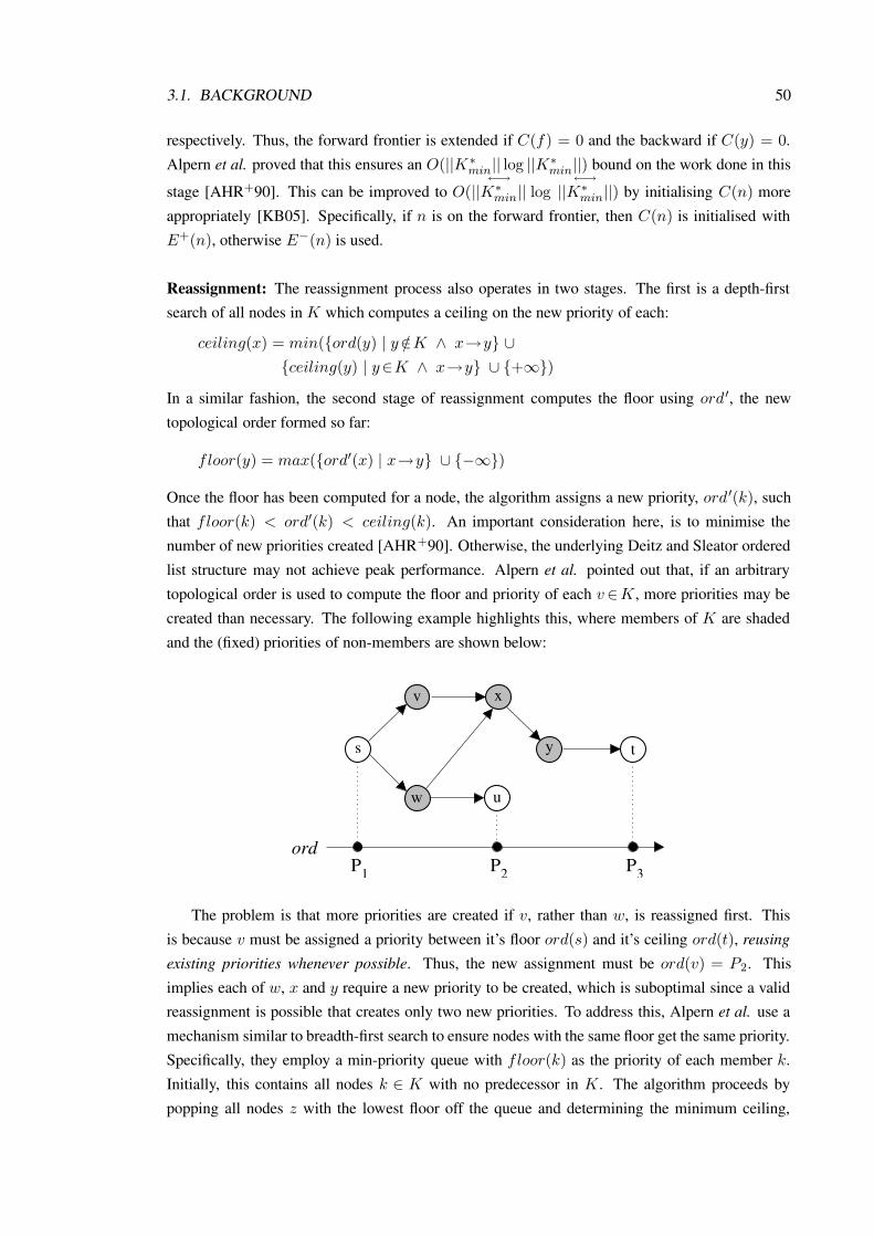
3.1. BACKGROUND 50

respectively. Thus, the forward frontier is extended if C(f) = 0 and the backward if C(y) = 0.

Alpern et al. proved that this ensures an O(||K ∗min|| log ||K∗min||) bound on the work done in this

stage [AHR+90]. This can be improved to O(←→

||K∗min|| log←→

||K∗min||) by initialising C(n) more

appropriately [KB05]. Specifically, if n is on the forward frontier, then C(n) is initialised with

E+(n), otherwise E−(n) is used.

Reassignment: The reassignment process also operates in two stages. The first is a depth-firstsearch of all nodes in K which computes a ceiling on the new priority of each:

ceiling(x) = min(ord(y) | y /∈K ∧ x→y ∪ceiling(y) | y∈K ∧ x→y ∪ +∞)

In a similar fashion, the second stage of reassignment computes the floor using ord ′, the new

topological order formed so far:

floor(y) = max(ord′(x) | x→y ∪ −∞)

Once the floor has been computed for a node, the algorithm assigns a new priority, ord ′(k), such

that floor(k) < ord′(k) < ceiling(k). An important consideration here, is to minimise the

number of new priorities created [AHR+90]. Otherwise, the underlying Deitz and Sleator ordered

list structure may not achieve peak performance. Alpern et al. pointed out that, if an arbitrary

topological order is used to compute the floor and priority of each v∈K , more priorities may be

created than necessary. The following example highlights this, where members of K are shaded

and the (fixed) priorities of non-members are shown below:

1P 2P 3P

u

x

y

ord

ts

w

v

The problem is that more priorities are created if v, rather than w, is reassigned first. This

is because v must be assigned a priority between it’s floor ord(s) and it’s ceiling ord(t), reusing

existing priorities whenever possible. Thus, the new assignment must be ord(v) = P2. This

implies each of w, x and y require a new priority to be created, which is suboptimal since a validreassignment is possible that creates only two new priorities. To address this, Alpern et al. use a

mechanism similar to breadth-first search to ensure nodes with the same floor get the same priority.

Specifically, they employ a min-priority queue with floor(k) as the priority of each member k.

Initially, this contains all nodes k ∈ K with no predecessor in K . The algorithm proceeds by

popping all nodes z with the lowest floor off the queue and determining the minimum ceiling,

3.1. BACKGROUND 51

zmin, between them. Each z is then assigned the same priority Pz , where floor(z)<Pz<zmin.

In doing this, the lowest existing priority is always used when possible, otherwise a new priority

is created. At this point, all remaining nodes whose predecessors are either not in K or have

already been reassigned are pushed onto the queue. The whole process is repeated until all of K is

reassigned. For the above example, this procedure creates the minimum number of new priorities.

However, Alpern et al. did not prove that this holds for the general case, although it seems likely.

Finally, since all edges touching nodes in K must be scanned to generate the floor and ceiling

information, the time needed for this stage is bounded by O(||K ∗min|| + K∗min logK∗min). The

log factor arises from the use of a min-priority queue. In fact, Katriel and Bodlaender showed

that this can be reduced to O(K∗min), using a simpler mechanism [KB05]. However, this does not

minimise the number of new priorities created and, thus, is expected to perform worse in practice.

The original bound given by Alpern et al. on the total time needed to process an edge insertion

was O(||K∗min|| log ||K∗min||) [AHR+90, RR94]. However, it is easy to see that this reduces to

O(←→

||K∗min|| log←→

||K∗min||) if the improved discovery algorithm and the simple O(K ∗min) approach

to reassignment are used. Pseudo-code for our implementation is provided in Figure 3.3 and there

are a few remarks to make about it. In particular, the improved discovery algorithm of Katriel and

Bodlaender is used, although their simpler reassignment algorithm is not — even though it offers

lower time complexity. As discussed above, this is because their approach does not minimise the

number of new priorities created and, hence, is expected to perform poorly in practice [AHR+90].

There are also a few points to make about the Dietz and Sleator ordered list structure [DS87]

which AHRSZ relies on: firstly, it is difficult to implement and suffers high overheads in practice

(both in time and space); secondly, only a certain number of priorities can be created for a given

word size, thus limiting the maximum number of nodes. In fact, the original paper by Dietz and

Sleator developed three ordered list algorithms: the first has an amortised O(log n) time bound

and holds up to 32768 priorities with 32 bit integers; the second has an amortised O(1) time bound

and holds 220 priorities with 32bit integers; the third has a worst-case O(1) time bound. Generally,

we consider the second variant to be of most practical value for this work. In particular, while we

find the first variant to have lower time overheads, its limit on the maximum number of priorities

is too restrictive. For example, up to 63568 priorities are needed to analyse ghostscript with our

basic flow-insensitive pointer analysis (see Table 4.1, Chap 4) and even more are required for thefield-sensitive version. In addition, we choose the second ordered list variant over the third in

spite of its worse time complexity, as Dietz and Sleator themselves expect it to perform better in

practice.

Finally, while we have studied the main aspects of algorithm AHRSZ here, some additional

results are known. Katriel and Bodlaender showed that O(minm3/2 log v,m3/2 +v2 log v) time

is needed to process a sequence of m edge insertions [KB05]. They also found that, for DAGs

with treewidth k, the modified algorithm needs at most O(mk log2 v) time to insert m edges and

that, for the special case of trees, this reduces to O(v log v). Zhou and Muller have also shown the

space requirements of AHRSZ can be reduced [ZM03].

3.1. BACKGROUND 52

procedure add edge(x, y)if ord(y) ≤ ord(x) then K = ∅; discovery(); reassignment();

procedure discovery()ForwFron = y; f = y; BackFron = x; b = x;ForwEdges = OutDegree(f); BackEdges = InDegree(b);// extend frontiers until either one is empty or they meetwhile ord(f) ≤ ord(b) dou = min(ForwEdges,BackEdges);ForwEdges = ForwEdges− u;BackEdges = BackEdges− u;if ForwEdges = 0 then

// extend forward frontierK ∪= f; ForwFron −= f;forall f→y ∈ E do ForwFron ∪= y;if ForwFron = ∅ then f = x;else f = ForwFron.top();ForwEdges = OutDegree(f);

if BackEdges = 0 then// extend backward frontierK ∪= b; BackFron −= b;forall y→b ∈ E do BackFron ∪= y;if BackFron = ∅ then b = y;else b = BackFron.top();BackEdges = InDegree(b);

procedure reassignment()// compute ceilingsforall x ∈ K in reverse topological order do

ceiling(x) = +∞;forall x→y ∈ E do

if y ∈ K then ceiling(x) = min(ceiling(y), ceiling(x));else ceiling(x) = min(ord(y), ceiling(x));

// compute new priorities, whilst minimising number createdQ = ∅;forall x ∈ K do

deps(x) = |u | u→x ∧ u∈K|;if deps(x) = 0 then floor(x) = max(ord(y) | y→x ∈ E ∪ −∞); Q.push(x);

while Q 6= ∅ doZ = z ∈ Q | floor(z) = floor(Q.top());Pz = compute priority(floor(Q.top()),min(ceiling(z) | z∈Z));forall z ∈ Z doord(z) = Pz; Q.pop();forall z→u ∈ E where u∈K do

deps(u) = deps(u)− 1;if deps(u) = 0 then floor(u) = max(ord(y) | y→u ∈ E ∪ −∞); Q.push(u);

procedure compute priority(floor, ceiling)// select lowest priority z where floor < z < ceiling// if none exists then create one in O(1) timereturn z;

Figure 3.3: Algorithm AHRSZ, an optimal solution for the (unit change) DTO problem. The for-ward frontier is represented by ForwFron, and implemented using a min-priority queue. BackFronis similar, but using a max-priority queue. Notice that ForwEdges and BackEdges implement thecounter C(n) discussed in the text. Finally, Q is implemented using a min-priority queue.

3.2. ALGORITHM PTO1 53

3.2 Algorithm PTO1

We now present our first algorithm for solving the DTO problem. The development of this came

from efforts to improve upon MNR and, hence, they share many similarities. The main improve-

ment is a much tighter bound on the time needed for an edge insertion. While this remains inferiorto that of AHRSZ, our claim is that its simplicity makes it more efficient in practice. In particular,

the complicated Dietz and Sleator ordered list structure is not used. Like the others, PTO1 is a unit

change algorithm operating on directed acyclic graphs.

The topological ordering, ord, is implemented as a total and contiguous ordering using an

array of size |V |. As with MNR, this maps each vertex to a unique integer in 1. . .|V |, such that

for any edge x→ y, ord(x) < ord(y) always holds. A second array (i.e. ord−1) is not used.

Thus, PTO1 has the lowest storage requirements of any so far2. The main observation behind the

algorithm is that, for an invalidating edge insertion x→ y, we can obtain a correct ordering by

simply reorganising nodes in δxy . That is, in the new ordering ord′, nodes in δxy are repositioned

to ensure a valid topological ordering, using only positions previously held by members of δxy . All

other nodes remain unaffected and this represents a significant departure from MNR, where the

entire affected region is reorganised. Consider the following example, arising from an invalidating

edge insertion x→y:

y a b c x

affected region

As before, nodes are laid out in topological order from left to right. Only members of δxy are

shown and, as ord is total and contiguous, the gaps must contain nodes omitted to simplify the

presentation. So, we have δ+xy = y, a, c and δ−xy = b, x and we obtain a correct ordering by

repositioning nodes to ensure all of δ−xy are left of δ+xy:

b x y a c

In doing this, the original (relative) order of nodes in δ+xy must be preserved and likewise for δ−xy.

2In fact, this is only true if the underlying graph data structure is an adjacency matrix. When an adjacency list isused, PTO1 may need more space than MNR (but not AHRSZ), because it necessitates a bidirectional adjacency listwhere MNR does not. This is because PTO1 relies on the ability to efficiently traverse both inedges and outedges, whileMNR only ever traverses outedges.


This ensures that the following subtle invariant is maintained, where ord ′ is the new ordering being

computed:

∀x∈δ+xy.[ord(x) ≤ ord′(x)

]∧ ∀y∈δ−xy.

[ord′(y) ≤ ord(y)

]

The above states that members of δ+xy cannot be given lower priorities than they already have,

whilst those in δ−xy cannot get higher ones. This is because, for any node in δ+xy , we have identified

all in the affected region which must be higher than it (i.e. right of it). However, we have not

determined all those which must come lower and, hence, cannot safely move them in this direction.

A similar argument holds for δ−xy . Thus, we begin to see how the algorithm works: it first identifies

δ−xy and δ+xy . Then, it pools the indices occupied by their nodes and, starting with the lowest,

allocates increasing indices first to members of δ−xy and then δ+xy . So, in the above example, the

algorithm proceeds by allocating b the lowest available index, like so:

affected region

b x a cy

? ? ? ? ?

After this, it will allocate x to the next lowest index, then y and so on. The algorithm is pre-sented in Figure 3.4 and the following summarises the two stages:

Discovery: The set δxy is identified using a forward depth-first search from y and a backward

depth-first search from x. Nodes outside the affected region are not explored. Those visited by the

forward and backward search are placed into δ+xy and δ−xy respectively. Thus, exactly Θ(

←→||δxy||)

time is needed for this stage.

Reassignment: The two sets are now sorted separately into increasing topological order (i.e.

according to ord), which we assume takes Θ(δxy log δxy) time. We then load δ−xy into array L

followed by δ+xy . In addition, the pool of available indices, R, is constructed by merging indices

used by elements of δ−xy and δ+xy together. Finally, we allocate by giving index R[i] to node L[i].

This whole procedure takes Θ(δxy log δxy) time.

Therefore, algorithm PTO1 has time complexity Θ((δxy log δxy)+←→||δxy||), which is a good im-

provement over MNR, but remains marginally inferior to AHRSZ. As it is a unit change algorithm(i.e. it offers no advantage to processing in batches) PTO1, like the others studied so far, requires

O(b(v + e)) time to process a batch of b insertions. Elsewhere, Katriel has also demonstrated this

algorithm to be worse-case optimal with respect to the number of nodes reordered over a series of

edge insertions [Kat04a]. Finally, we provide the necessary correctness proof of algorithm PTO1:


Lemma 5. Assume D = (V,E∪x→y) is a DAG and ord an array, mapping vertices to unique

values in 1 . . . |V |, which is a valid topological order of E. For an invalidating edge insertion,

x→y, algorithm PTO1 obtains a correct topological ordering.

Proof. Let ord′ be the new ordering found by the algorithm. To show this is a correct topological

order we must show, for any two vertices a, b where a→ b, that ord′(a) < ord′(b) holds. An

important fact to remember is that the algorithm only uses indices of those in δxy for allocation.

Therefore, z∈δxy ⇒ ord(y) ≤ord′(z)≤ord(x). There are six cases to consider:

(i) a, b /∈ARxy . Here neither a nor b have been moved as they lie outside affected region. Thus,

ord(a)=ord′(a) and ord(b)=ord′(b) which (by defn of ord) implies ord′(a) < ord′(b).

(ii) (a ∈ ARxy∧b /∈ ARxy) ∨ (a /∈ ARxy∧b ∈ ARxy). When a ∈ ARxy we know ord(a) ≤ord(x) < ord(b). If a∈δxy then ord′(a)≤ord(x). Otherwise, ord′(a)=ord(a). A similar

argument holds when b∈ARxy.

(iii) a, b∈ARxy ∧ a, b /∈δxy. Similar to case 1 as neither a or b have been moved.

(iv) a, b∈ δxy ∧ x; a ∧ x 6= a. Here, a reachable from x only along x→ y, which means

y;a ∧ y;b. Thus, a, b∈δ+xy and their relative order is preserved in ord′ by sorting.

(v) a, b∈δxy ∧ b;y ∧ y 6=b. Here, b reaches y along x→y, so b;x and a;x. Therefore,

a, b ∈ δ−xy and their relative order is preserved in ord′ by sorting.

(vi) x = a ∧ y = b. Here, we have a∈δ−xy ∧ b∈δ+xy and ord′(a) < ord′(b) follows because all

elements of δ−xy are allocated lower indices than those of δ+xy .


procedure add edge(x, y)lb = ord[y];ub = ord[x];if lb < ub then

// Discoverydfs-f(y);dfs-b(x);// Reassignmentreorder();

procedure dfs-f(n)visited(n) = true;δ+xy ∪= n;

forall n→w ∈ E doif ord[w] = ub then abort; //cycle// is w unvisited and in affected region?if ¬visited(w) ∧ ord[w]<ub then dfs-f(w);

procedure dfs-b(n)visited(n) = true;δ−xy ∪= n;forall w→n ∈ E do

// is w unvisited and in affected region?if ¬visited(w) ∧ lb<ord[w] then dfs-b(w);

procedure reorder()// sort sets to preserve original order of elementssort(δ−xy);sort(δ+

xy);L = ∅;

// load δ−xy onto array L firstfor i = 0 to |δ−xy|−1 dow = δ−xy[i];δ−xy[i] = ord[w];visited(w) = false;push(w,L);

// now load δ+xy onto array L

for i = 0 to |δ+xy|−1 do

w = δ+xy[i];

δ+xy[i] = ord[w];

visited(w) = false;push(w,L);

merge(δ−xy , δ+xy, R);

// allocate nodes in L starting from lowestfor i = 0 to |L|−1 do ord[L[i]] = R[i];

Figure 3.4: The PTO1 algorithm. The “sort” function sorts an array such that x comes before y ifford[x] < ord[y]. “merge” combines two arrays into one whilst maintaining sortedness (i.e. mergesort).


3.3 Algorithm PTO2

We now present our second algorithm, referred to as PTO2, for dynamically maintaining the topo-

logical order of a DAG. This is the first batch algorithm for this problem and, hence, it can be

considerably more efficient than any considered so far when edges are added in batches. Like

PTO1, it is similar in design to MNR, this time employing both arrays, ord and ord−1, to map

nodes to indices and vice-versa. In fact, when only a single edge is added at a time, the algorithm

operates in an identical fashion to MNR. So, our starting point is to identify where MNR performs

redundant work when processing in batches. Consider the following, where there are two invali-

dating edges:

affected region 1

y vbw a x

affected region 2

To deal with this batch update problem, each edge must be passed to MNR one at a time. If

x→y is first, then applying MNR yields the following intermediate solution:

affected region 2

vw b x y a

As expected, y and a were visited during the discovery (i.e. depth-first search) phase of MNR

and then shifted past x. Now, inserting the second edge v→w means that w, b, x, y and a are all

visited by the discovery phase and shifted past v to obtain the final solution:

ayxbwv

Thus, we see that a is discovered and shifted twice — once when x→ y was added and then

again for v→w. Furthermore, every node which was originally in both affected regions has also

been shifted twice. This is unnecessary as, by looking at the final solution, we know that every

node which was originally left of and reachable from v must be shifted right of it. Hence, had we


somehow determined this set of nodes beforehand then only one shift would have been required.

Note that, inserting v→w before x→y does not prevent nodes from being shifted twice.

The key feature of algorithm PTO2 is that it never visits or shifts a node more than once when

inserting a batch of edges. In order to achieve this, we must alter our notion of the affected re-

gion, which was previously defined as the set of nodes between the head and tail of an invalidating

edge. This is done by treating overlapping regions as one — so, although a batch of insertions can

still define several affected regions, they are all distinct and can be processed independently. Thefollowing aims to clarify the new definition of an affected region:

affected region 3

a b c d e f g h i

affected region 2affected region 1

Here, each affected region can be correctly ordered independently of the others, by simply

rearranging its contents. The difficulty then, lies in rearranging an individual region without vis-

iting or shifting any node twice. This is complicated by the fact that we must now shift nodes to

different points within an affected region, instead of only to the rightmost positions (as done inMNR). For example, in the above, f must be positioned just right of h, whilst g must go next to i.

In fact, the reader may wonder why we don’t simply shift both f and g past i. Doing this, it turns

out, requires more work as we must also identify and shift any node reachable from f between

h and i. Therefore, we introduce the shift queue which is a LIFO queue of tuples, 〈x, d〉, where

x is to be shifted past d (its destination). For example, the shift queue for processing region 3

above would be: 〈f, h〉, 〈g, i〉. The shifting process operates in much the same way to that of

MNR — by scanning the region from left-to-right whilst filling up vacant slots by moving those

not being shifted to the left. One difference is that, after moving a node, we check whether it is

the destination of any on the shift queue and, if so, place them immediately after it. The following

elaboration of region 3 from above shows how it would be shifted using this process:

wh ix y z izx y h

<g,i><f,h>

shift queue

w

At this point, the algorithm has just moved h to the left and, as its destination has been reached,

f will be placed into the free slot following it. The algorithm will then proceed by moving z and i

one slot to the left and then placing g. Notice how the queue is carefully arranged so tuples whose


destinations will be encountered first are on top. Thus, only a constant-time check is needed to

determine whether nodes on the queue need to be placed or not.

At this point, the remaining difficulty is with the discovery stage of the algorithm which is

responsible for loading the shift queue before each region is reordered. The goal is to ensure each

node in the region is visited at most once and the key to achieving this lies in the order with which

invalidating edges are processed. Recall the discovery procedure of MNR consists of searching

from the head of the invalidating edge to identify and mark those which must be shifted past its

tail. The new procedure remains similar to this, in that we pick an invalidating edge x→ y and

then search forward from y. This time, however, discovered nodes are placed onto the shift queue,

raising the question of what destination to give them. Unfortunately, the obvious answer of using

the tail of the invalidating edge does not necessarily work. For example, consider the following

graph:

affected region

y vxw

Now, suppose we begin with x→ y by searching forward from y (within the affected region)

and adding all encountered to the shift queue. The problem is that the destination for these nodes

is actually v, not x, but we cannot know this before processing v→w. Therefore, PTO2 processes

invalidating edges in decreasing order by the topological index of their tail. In other words, it

processes them from right to left. This guarantees it to always start at the rightmost point of any

series of connected invalidating edges. Furthermore, if an invalidating edge is traversed (e.g. x→y

above) whilst processing another (e.g. v→w above) then it will not be considered again.

A subtle point, worth mentioning here, is the way in which the searching is pruned. In the orig-

inal MNR algorithm, each search was simply restricted to be within the affected region. However,

using this rule with our new definition of an affected region leads to some inefficiency:

affected region

f g h i

Here, f connects to a number of nodes right of h and, as they lie in the affected region, it

seems that a search from f should visit them. However, it turns out that, since h is the destination


of those discovered from f , only nodes between f and h need to be visited. Therefore, algorithm

PTO2 restricts the search to all nodes whose index is lower than the current destination (h in this

case).

Pseudo-code for algorithm PTO2 is provided in Figure 3.5 and we now consider its worse-case

time complexity over a batch of b edge insertions. If we assume that sort is implemented using

a merge sort, then the worse case runtime is O(v + e + b. log b) as the algorithm can visit each

node at most twice (once whilst searching and once whilst shifting). In fact, thanks must go to Irit

Katriel for pointing out that this can be improved to O(v + e+ b) if a bucket sort is used instead

[Kat04b]. Thus, we see that PTO2 offers a dramatic improvement over the O(b(v + e)) bound

obtained for the other algorithms studied in this chapter.

The final part remaining in our discussion of algorithm PTO2 is to provide the necessary

correctness proof. Perhaps unsurprisingly, this is a difficult undertaking and, as is customary, we

aim only to provide enough detail to convince the reader of the algorithm’s correctness. The center

piece of the proof is the shift queue since this is really the glue connecting the discovery stage of

the algorithm with the shifting stage.

Lemma 6. Assume D = (V,E ∪B) is a DAG and ord an array mapping each vertex to a unique

index from 1 . . . |V | which is a valid topological order ofE, with ord−1 implementing its reverse

map. For a batch B of edge insertions, algorithm PTO2 produces a valid topological ordering.

Proof. Let ord’ be the new value of ord computed by the algorithm. Now, let us assume that ord’

is not a valid topological ordering of nodes. Hence, there must exist two nodes, v and w, for which

v;w and ord’(w) < ord’(v) is true. There are five cases to consider and we now demonstrate

how each yields a contradiction of our assumptions:

(i) Neither v nor w were placed on the shift queue, Q, and ord(v) < ord(w). Since shift

is only incremented when a visited node (i.e. a member of Q) is reached, any two nodes

i, j /∈ Q must retain their relative ordering and, hence, ord′(v) < ord′(w).

(ii) Neither v nor w were placed on the shift queue and ord(v) > ord(w). Since ord is a valid

ordering for all edges except those in B, v can only reach w by some series of invalidating

edges. Let x→ y be the invalidating edge whose tail has the highest priority of any on a

path from v to w. As invalidating edges are sorted into decreasing order by the priority of

their tail, it follows that dfs(y, ord(x)) will be invoked before dfs(z, . . .), for any other node

z on a path from v to w. Furthermore, it must hold that ord(v) ≤ ord(x) — otherwise vcould not reach w as (by definition of x) there are no invalidating edges higher up than x.

From this and the basic properties of depth-first search it follows that dfs(y, ord(x)) invoked

dfs(w, ord(x)), thus placing w onto the shift queue and contradicting our assumption.

(iii) 〈w, z〉 was placed on the shift queue, but 〈v, . . .〉 wasn’t. From this, ord(w) < ord(z)

immediately follows. Now, if ord(v) ≤ ord(z) then the contradiction follows easily as w

is placed (possibly along with other members of the shift queue) immediately after z. If

ord(v) > ord(z) then there must be an invalidating edge x→ y where ord(z) < ord(x)


procedure add edges(B)// remove forward edges from Bforall x→y ∈ B do if ord[x] < ord[y] then B −= x→y// sort invalidating edges into descending order by index of their tailsort(B);Q = ∅; // the shift queuelb = |V |; // lowerbound of current affected region// process invalidating edgesfor i = 0 . . . |B| dox→y = B[i];// if index of tail less than lower bound, current region finished, so shiftif ord[x] < lb then shift(lb);// dfs from head if edge not already traversedif ¬visited(y) then dfs(y, ord[x]);lb =min(ord[y], lb);

// shift final affected regionshift(lb);

procedure dfs(n, ub)visited(n) = true;forall n→s ∈ E do

if ord[s] = ub then abort; // cycle detected// visit s if not already and is in affected regionif ¬visited(s) ∧ ord[s]<ub then dfs(s, ub);

// place n and current destination in topological order on queuepush(〈n, ord−1[ub]〉, Q)

procedure shift(i)shift = 0;while Q 6=∅ dow = ord−1[i]; // w is node at topological index iif visited(w) then

visited(w) = false;shift=shift+1;

else allocate(w, i − shift);// now insert all nodes associated with index i〈n, t〉 = top(Q);while Q 6=∅ ∧ w = t doshift=shift−1;allocate(n, i − shift);pop(Q);〈n, t〉 = top(Q);

i = i+1;

procedure allocate(n, i)// place n at index iord[n] = i; ord−1[i] = n;

Figure 3.5: Algorithm PTO2. This first marks those nodes reachable from y in ARxy and thenshifts them to lie immediately after x in ord−1. Note that, initially all nodes are marked unvisited.


and x ; w, because otherwise v 6; w. As invalidating edges are sorted into decreasing

order by the priority of their tail, dfs(y, ord(x)) must have been invoked before dfs(u, . . .),

for any other node on a path v ; w. Thus, it again follows from the basic properties of

depth-first search that dfs(y, ord(x)) invoked dfs(w, ord(x)). This gives the contradiction,

since it implies that 〈w, x〉 was placed onto the shift queue (not 〈w, z〉).

(iv) 〈v, z〉 was placed on the shift queue, but 〈w, . . .〉 wasn’t. From this, ord(v) < ord(z)

immediately follows. Now, if ord(w) < ord(z) then dfs(v, ord(z)) (which must have been

called for v to be on the shift queue) would have lead to dfs(w, ord(z)) and w being pushed

on the shift queue, giving the contradiction. If ord(z) ≤ ord(w) then 〈z, x〉 was not placed

on the shift queue, for any node x. This holds because otherwise 〈v, x〉 would have been

pushed onto the queue (since x;v ∧ ord(z) < ord(x) and a similar argument to that used

in (ii) and (iii) applies). Furthermore, since neither z nor w are placed on the shift queue,

the argument from (i) gives ord′(z) < ord′(w). Thus, a contradiction is obtained as v is

placed (possibly with other members of the shift queue) immediately after z.

(v) Both 〈v, x1〉 and 〈w, x2〉 were placed on the shift queue. Again, ord(v) < ord(x1) ∧ord(w) < ord(x2) follows immediately. If it can be shown that 〈v, x1〉 is pushed onto

the queue after 〈w, x2〉, then the contradiction follows easily because nodes are allocated

in LIFO order. Thus, it remains only to show this. Let x1→ y1 and x2→ y2 be the two

invalidating edges responsible for pushing 〈v, x1〉 and 〈w, x2〉 onto the queue respectively.

If x1 = x2 then either dfs(v, ord(x1)) invoked dfs(w, ord(x1)) or the latter had already

been called (due to some path x1 ;w not involving v). Either way, 〈w, ord(x1)〉 is pushed

first. If x1 6= x2 then either ord(x1) < ord(x2) and dfs(w, ord(x2)) was invoked first,

or ord(x1) > ord(x2) and dfs(v, ord(x1)) failed to call dfs(w, ord(x1)). For the latter to

hold, it must be that ord(x1) < ord(w) (otherwise w was already visited). But, this implies

ord(x1) < ord(x2) and, hence, that dfs(w, ord(x2)) was invoked before dfs(v, ord(x1)).

Again, both cases result in 〈w, ord(x1)〉 being pushed first.

3.4. EXPERIMENTAL STUDY 63

3.4 Experimental Study

In this section, we experimentally compare five algorithms for the DTO problem: MNR, AHRSZ,

PTO1, PTO2 and STO (recall Figure 3.1). The experiments measure how the Average Cost Per

Insertion (ACPI) varies with graph density and batch size, over a large number of randomly gen-

erated DAGs.

Definition 8. For a DAG with v nodes and e edges, define its density to be e12v(v−1)

. Thus, it is the

ratio of actual edges to the maximum possible.

Furthermore, in an effort to correlate with our theoretical analysis, we also investigated how←→||δxy||, |ARxy| and

←→||K||, where K is the actual cover computed by AHRSZ, vary on average with

graph density.

3.4.1 Generating a Random DAG

The standard model for generating a random undirected graph is G(v, p), which defines a graph

with v vertices where each edge is picked with probability p. Erdos and Renyi were the first to

study this random graph model [ER60]. They found that, for certain properties such as connect-

edness, graphs whose edge count was below a certain threshold were very unlikely to have the

property, whilst those with just a few more edges were almost certain to have it. This is known as

the phase transition and is a curious and pervasive phenomenon (see [JLR00, Chapter 5] for more

on this). Several other random graph models exist, such as one for generating graphs which obey

a power law [ACL00]. For this work, we are only concerned with generating random DAGs and

the model Gdag(v, p), first defined by Barak and Erdos [BE84], is used here:

Definition 9. The model Gdag(v, p) is a probability space containing all graphs having a vertex

set V = 1, 2, . . . , v and an edge set E ⊆ (i, j) | i < j. Each edge of such a graph exists with

a probability p independently of the others.

For a DAG in Gdag(v, p), we know that there are at most v(v−1)2 possible edges. Thus, we can

select uniformly fromGdag(v, p) by enumerating each possible edge and inserting with probability

p. In our experiments, we used p = x to generate a DAG with v nodes and expected density x.

The approach to generating random DAGs suggested here is by no means the only method.

One alternative is to use a Markov Chain where each step consists of picking two nodes at random

and either deleting the edge between them (if one is present) or inserting an edge between them (if

one is not) [MBMD01, IC02]. Note that, if inserting an edge would introduce a cycle then nothing

is done. In general, it remains unclear how the two generation methods compare and further work

could examine this in more detail.An interesting aspect of our random DAGs is how they are affected by the phase transition and

this issue was addressed by Pittel and Tungol [PT01]. They showed that, if p = c(ln v)v , then the

size of the largest transitive closure of any vertex (i.e. the vertex with most edges after closure)

is asymptotic to vc ln v, 2v(ln ln v)v and v(1 − 1

c ), when c < 1, c = 1 and c > 1 respectively.

This means the phase transition occurs roughly at a graph density of ln vv , after which point it is


procedure measure acpi(v, d, b, s)// v = number of nodes, d = density, b = batch size, s = sample SizeES = . . . ; // generate d. 12v(v−1) random (acyclic) edgesS = randomly select s. 12v(v−1) edges from ES;

G = (1 . . . v, ES−S);start = timestamp();while S 6= ∅T = randomly select b edges from S;S = S − T ;add edges(T,G);

return 1|S| .(timestamp()− start);

Figure 3.6: Our procedure for measuring insertion cost over a random DAG. Note that, throughcareful implementation, we have minimised the cost of the other operations in the loop, whichmight have otherwise interfered. In particular, the order in which edges are picked from S isprecomputed, using a random shuffle.

likely that a path exists from the root (i.e. that with the lowest index in our model) to every other

node. In the experiments which follow, the graphs normally have 2000 nodes and, thus, the phase

transition should occur around 0.0038. For this reason, we consider graphs with density below

this threshold as sparse, and those over it as dense.

3.4.2 Experimental Procedure

Our general procedure for measuring the Average Cost Per Insertion (ACPI) for an algorithm

was to generate, for some v and density, a random DAG and measure the time taken to insert a

sample of edges whilst maintaining a topological order. Figure 3.6 outlines the procedure. Note,

the sample size was fixed at 0.0001 (i.e. 0.01% of all 12v(v − 1) possible edges). Although

this seems like a small number, it is important to realise that most of the interesting observations

occur between 0.001 and 0.02 density and, thus, larger sample sizes would swamp our results.

To generate each data point, we averaged over 100 runs of this procedure (i.e. over 100 random

DAGs). An important aspect of our procedure is that the sample may include non-invalidating

edges and these dilute our measurements, since all five algorithms do no work for these cases.

Our purpose, however, was to determine what performance can be expected in practice, where it

is unlikely all edge insertions will be invalidating.

As mentioned already, some of our experiments measured the average set size of our complex-

ity metrics, instead of ACPI. The procedure for doing this was almost identical to before except,

instead of measuring time, exact values for←→||K||,

←→||δxy|| and |ARxy| were recorded. These were

obtained from the corresponding algorithm (AHRSZ for←→||K||, PTO1 for

←→||δxy|| and MNR for

|ARxy|) by counting nodes visited and edges iterated where appropriate.

Finally, all experiments were performed on a 900Mhz Athlon based machine with 1GB of

main memory, running Redhat Linux 8.0. The executables were compiled using gcc 3.2, with


optimisation level “-O3” and timing was performed using the gettimeofday function, which

gives microsecond resolution. To reduce interference, experiments were performed with all non-

essential system daemons/services (e.g. X windows, crond) disabled and no other user-level

programs running. The implementation itself was in C++ and took the form of an extension to the

Boost Graph Library [SLL02] and utilised the adjacency_list class to represent the DAG.

Our implementation of AHRSZ employs the O(1) amortised (not O(1) worse-case) time structure

of Dietz and Sleator [DS87]. This seems reasonable as they themselves state it likely to be more

efficient in practice.

3.4.3 Single Insertion Experiments

The purpose of these experiments was to investigate the performance of the three unit change algo-

rithms, AHRSZ, PTO1 and MNR. Specifically, we looked at how ACPI varied with graph density

and we report our findings here. Furthermore, we include data for a control experiment (labelled

as CTRL), whose purpose is to indicate the best possible performance any algorithm could obtain.

To generate data for our control, we perform exactly the same steps as for the other algorithms,

except that no work is done to actually maintain the topological order. Thus, the control measures

the cost of inserting edges into our underlying graph data structure.

Figure 3.7 shows the effect on ACPI and the complexity parameters of varying density, whilst

maintaining |V | constant. Although the highest density shown is 0.1, we have explored beyond

this and found the plots extend as expected. Therefore, we limit our attention to this density range

as it is most interesting. From the topmost graphs, we see that all three algorithms have quite dif-

ferent behaviour. The main observations are: firstly, MNR performs poorly on sparse graphs, but is

the most efficient on dense graphs; secondly, PTO1 performs well on very sparse and dense graphs,

but not as well on those inbetween; finally, AHRSZ is relatively poor on very sparse graphs, butotherwise has constant performance which is reasonably competitive with the others. By looking

at the middle two graphs of Figure 3.7, a clear resemblance can be seen between the plots of ACPI

for PTO1 and←→||δxy||, between that for MNR and |ARxy| and between that for AHRSZ and

←→||K||.

Also, it is interesting to note that, while←→||K|| is generally much smaller than

←→||δxy||, AHRSZ still

performs worse than PTO1 and this reflects the larger constants involved in its implementation.

Clearly, the curves observed for the three complexity metrics are key to understanding the

performance of the algorithms. Their shape can be explained if we consider the number of in-

validating edges in the insertion sample. The bottom two graphs of Figure 3.7 plot this and they

show that the proportion of invalidating edges goes down rapidly with density. But, why is this?

Well, we know that as density increases, the chance of a path existing between any two nodes

must also increase. From this, it follows that the number of possible invalidating edges must go

down as density goes up. This is because an edge x→ y is invalidating only if there is no path

from x to y. The steepness of these plots is governed by the phase transition phenomenon, which

dictates that the chance of a path existing between two nodes quickly approaches 1 as soon as the

0.0038 density threshold is passed. From these facts, the curves seen for |ARxy| and←→||δxy|| can


0

5

10

15

20

0 0.02 0.04 0.06 0.08 0.1

Ave

rage

Cos

t Per

Inse

rtion

(us)

Graph Density

|V|=2000

PTO1AHRSZ

MNRCTRL

0

1

2

3

4

5

0 0.01 0.02 0.03 0.04 0.05

Ave

rage

Cos

t Per

Inse

rtion

(us)

Graph Density

|V|=2000 (close up)

PTO1AHRSZ

MNRCTRL

0

2

4

6

8

10

12

14

0 0.02 0.04 0.06 0.08 0.1

Ave

rage

Set

Siz

e

Graph Density

|V|=2000

||K<->|||ARxy|

||δxy<->||

0

2

4

6

8

10

12

14

0 0.005 0.01 0.015 0.02

Ave

rage

Set

Siz

e

Graph Density

|V|=2000 (close up)

||K<->|||ARxy|

||δxy<->||

0

20

40

60

80

100

0 0.01 0.02 0.03 0.04 0.05 0.06 0.07 0.08 0.09 0.1

Per

cent

age

of S

ampl

e

Graph Density

|V|=2000

#Invalidating (PTO1)

0

10

20

30

40

50

60

70

80

90

100

0 0.01 0.02 0.03 0.04 0.05 0.06 0.07 0.08 0.09 0.1

Per

cent

age

of S

ampl

e

Graph Density

|V|=2000

#Invalidating (AHRSZ)

Figure 3.7: Experimental results for random DAGs with 2000 nodes of increasing density. Thetopmost plots show ACPI against density for the three unit change algorithms and our control.The middle plots show the complexity metrics which measure the work done by each algorithm.Finally, the bottom plots illustrate how the proportion of the insertion sample which is invalidatingdecreases with density for PTO1 and AHRSZ.


be explained: firstly, the average size of an affected region must go down as density increases,

since |ARxy| = 0 for non-invalidating edges; secondly, the average size of←→||δxy|| must (initially)

increase with density, since its size is determined by the chance of a path existing between two

nodes. However, the decreasing number of invalidating edges will eventually overpower this and,

hence,←→||δxy || is determined by the trade-off between these two factors. The shape seen for

←→||K||

is more subtle. We had expected to see something more closely resembling that of←→||δxy||. That

is, we had expected to see←→||K|| go up initially and then fall. In fact, a small positive gradient can

be seen roughly between 0.001 and 0.005 density which, we argue, corresponds to the increasing

chance of a path existing between two nodes at this point. The most important feature of this plot,

namely the negative initial gradient, is more curious. In particular, it seems strange that←→||K|| is

ever larger than←→||δxy||. This does make sense, however, if we contrast the bottom two graphs of

Figure 3.7 against each other. What we see is that the proportion of invalidating edges for AHRSZ

starts at a much higher point than for PTO1. This arises because, on very sparse graphs, AHRSZ

will assign most nodes the same priority — so most insertions are invalidating. In contrast, for

PTO1, all nodes have a different priority, regardless of density. This means there is (roughly) a

50% chance that any edge insertion x→ y will be invalidating, since y is equally likely to come

after x in the ordering than before it. Thus, as both←→||K|| and

←→||δxy|| are empty on valid insertions,

we can see that←→||δxy|| is smaller than

←→||K|| on very sparse graphs simply because it is measured

over fewer invalidating edges. Unfortunately, it still remains somewhat unclear why a negative

gradient is seen for←→||K||.

3.4.4 Experiment 2 - Batch Insertions

The purpose of these experiments was to investigate the benefits offered by algorithm PTO2, com-

pared with the others, when edges are inserted in batches. Furthermore, we were also interested in

seeing how it would compare against STO, which you may recall from Figure 3.1 uses a standard

(i.e. static) topological sort. So, following the same experimental procedure as before, we mea-

sured ACPI for all five algorithms for varying batch sizes on sparse and dense graphs.

Figure 3.8 shows the performance of PTO1, PTO2, MNR, AHRSZ and STO across varying batch

sizes at densities 0.0001, 0.001 and 0.01. The plots of the three unit change algorithms (i.e. PTO1,

MNR and AHRSZ) are flat as they can only process one edge at a time and, hence, obtain no ad-

vantage from seeing the edge insertions in batches. There are two overall conclusions from these

graphs: firstly, PTO2 is always a better choice than either MNR or STO and, in many cases, offers

a significant speedup; secondly, we find that PTO1 is very competitive with PTO2, even at largebatch sizes, which is perhaps unexpected. In particular, the topmost four graphs of Figure 3.8

illustrate that, on sparse graphs, PTO1 performs significantly better than PTO2. This stems from

the fact that PTO2 is a batch variant of MNR and, hence, shares its limitations on sparse graphs

— especially when the batch size is small. However, the bottom two graphs of Figure 3.8 confirm

that, on dense graphs, PTO2 is always the best choice when edges are inserted in batches.


0

20

40

60

80

100

120

140

0 20 40 60 80 100 120 140 160 180

Ave

rage

Cos

t Per

Inse

rtion

(us)

Batch Size

|V|=2000, density=0.0001

PTO1PTO2

AHRSZMNRSTO

0

5

10

15

20

25

30

0 20 40 60 80 100 120 140 160 180

Ave

rage

Cos

t Per

Inse

rtion

(us)

Batch Size

|V|=2000, density=0.0001 (close-up)

PTO1PTO2

AHRSZMNRSTO

0

20

40

60

80

100

120

140

160

0 40 80 120 160 200 240 280 320 360

Ave

rage

Cos

t Per

Inse

rtion

(us)

Batch Size

|V|=2000, density=0.001

PTO1PTO2

AHRSZMNRSTO

0

0.5

1

1.5

2

2.5

3

3.5

4

0 40 80 120 160 200 240 280 320 360

Ave

rage

Cos

t Per

Inse

rtion

(us)

Batch Size


PTO1PTO2

AHRSZSTO

0

20

40

60

80

100

120

140

160

0 40 80 120 160 200 240 280 320 360

Ave

rage

Cos

t Per

Inse

rtion

(us)

Batch Size

|V|=2000, density=0.01

PTO1PTO2

AHRSZMNRSTO

0

0.5

1

1.5

2

2.5

3

3.5

4

0 40 80 120 160 200 240 280 320 360

Ave

rage

Cos

t Per

Inse

rtion

(us)

Batch Size


PTO1PTO2

AHRSZMNR

Figure 3.8: Experimental results looking at the effect of increasing batch size for all five algorithmson random DAGs with 2000 nodes at densities 0.0001, 0.001 and 0.01. In each case, batch sizeis plotted against ACPI and we provide close ups at each density to capture interesting features.We were unable to explore batch sizes greater than 180 at density 0.0001, since these graphs musthave ≈ 200 edges after the insertion sample is completed. This limits the maximum batch sizeaccordingly, since it cannot be larger than the insertion sample.

3.5. DYNAMIC STRONGLY CONNECTED COMPONENTS 69

procedure dfs(n) // new edge is x→yvisited(n) = true;forall n→s ∈ E do

// visit s if not already and is in affected regionif ¬visited(s) ∧ ord[s]<ub then dfs(s);// back propagate component informationcomponent(n) = component(n) ∨ component(s);

Figure 3.9: The depth-first search component of MNR, modified to back-propagate componentinformation.

3.5 Dynamic Strongly Connected Components

In this section, we adapt algorithms MNR, PTO1 and PTO2 to the problem of (incremental) Dy-

namic Strongly Connected Components (DSCC). Henceforth, we refer to the new algorithms as

MSCC, PSCC1 and PSCC2 respectively. Furthermore, while the modifications are straightforward

and do not affect the complexity bounds obtained, we are unaware of any previous effort to use

this type of algorithm for dynamic cycle detection.

We begin by considering MNR and PTO1, since they are both extended in a similar way, based

on the following observation: if a new edge x→y introduces a cycle then x must be visited during

a forward depth-first search from y. Thus, it is easy enough to tell whether a cycle has been created

during the discovery stage of MNR or PTO1. The real question is: how can we identify members

of that cycle? By definition, all nodes reachable from y and reaching x are in the cycle, since

there is a path from each through x→ y back to itself. Therefore, we maintain an extra bit of

storage for each node, referred to as the component bit, indicating whether a node is in the cycle

or not. Initially, it is false for all nodes and, before starting the forward search from y, we set

component(x) = true. The idea now is to back-propagate component information along edgestraversed by the depth-first search. Figure 3.9 shows how the depth-first search used in MNR can

be modified for doing this.

Once a cycle has been detected we collapse its members into a single node and, hence, we

are effectively maintaining the topological order of the condensation graph. One issue is that,

since the topological ordering is maintained using arrays of size |V |, the collapsing process will

leave “unused slots” in the ordering — one per cycle member, less one for the representative. The

temptation maybe to reduce the size of the array in order to eliminate these, but doing so would

break our complexity bounds. Therefore, we simply leave them as is, since they can do no harm.

Figure 3.10 walks through an example, whilst Figure 3.11 provides pseudo-code for the extended

shift procedure from MNR. The extension for PTO1 is much the same, although care must be

taken to reset the visited flag for any nodes reached in dfs-f before moving onto dfs-b since

all predecessors of nodes in the component must be found to update the topological order correctly.

Detecting cycles with PTO2 is slightly harder, since multiple edges can introduce multiple

cycles, and the technique used for MNR and PTO1 no longer works. The solution is to combine

PTO2 with the original algorithm by Tarjan for detecting strongly connected components [Tar72].

3.5. DYNAMIC STRONGLY CONNECTED COMPONENTS 70

y xz uw

1. Initially, x is marked as component.

y xz uw

2. z is marked component, since it touches anode marked component.

xz uwy

3. Likewise, y is marked component, since italso touches a node marked component.

uw C

4. Finally, x, y, z are collapsed into one nodeC and shifted right as usual. This leaves two

blank slots which are not removed to preservethe complexity bound.

Figure 3.10: Illustrating algorithm MSCC operating on an example graph.

procedure shift() // new edge is x→yvisited(x) = false; component(x) = false;L = ∅; C = ∅; shift = 0;for i = lb to ub dow = ord−1[i]; // w is node at topological index iif visited(w) ∧ ¬component(w) then

push(w,L);shift = shift+1;visited(w) = false;

elseif component(w) then

push(w,C); // w is member of cyclecomponent(w) = false;visited(w) = false;

allocate(w, i−shift);// end for// place visited nodes after t in orderingfor j = 0 to |L| − 1 do

allocate(L[j], i−shift);i = i+1;

// check if new cycle detectedif |C| > 0 then collapse(x,C);

Figure 3.11: The extended shift procedure for algorithm MSCC. The “collapse(x,C)” functionmerges nodes in x ∪ C such that x becomes the representative in the underlying graph.


Since both algorithms use a depth-first search, it is very easy to compose them and this does not

affect the complexity bound obtained for PTO2. The main disadvantage over the simpler method

used for PTO1 and MNR is that Tarjan’s algorithm requires v(2+3w) additional storage bits, where

w is the word size and v the number of nodes. Note, Appendix B examines Tarjan’s algorithm in

detail and discusses some recent efforts to reduce the space requirements.


In this chapter, we have presented two new algorithms for dynamically maintaining a topological

order and have shown, through theoretical and experimental evaluation, that they improve upon the

best previously known works. In particular, we are the first to experimentally compare algorithms

for this problem. Furthermore, we have demonstrated that these algorithms can be extended to

detect strongly connected components dynamically, which is an important and well-known opti-

misation for pointer analysis.

While we have provided a detailed and rigorous analysis of algorithms for the DTO problem,

there remains several avenues which could be explored further. These include:

• Experimenting with real-world graphs. We are aware that uniform random graphs do not

necessarily reflect real life structures. Therefore, it would be interesting to experiment with

real-world graphs in an effort to see whether any difference arises. Indeed, any alternative

approach to generating the random graphs would also be interesting here.

• A bounded complexity result for PTO2. The reader may have noticed something interesting

about our analysis of algorithm PTO2 — we did not provide a result in terms of←→||δxy|| and

|ARxy|. This was not because we could not find one, but that we simply did not have time

to try. Furthermore, while the O(v + e + b) bound we give does improve upon that of the

three unit change algorithms, it does not in fact improve upon that of STO (recall Figure

3.1) which uses a standard (i.e. static) topological sort, but achieves the same worse case

bound. Nevertheless, we are confident that a result distinguishing PTO2 from STO can be

found, probably without much effort.

• Developing a batch variant of PTO1. Since we were able to find a batch variant of the MNR

algorithm, it seems plausible that a batch variant of PTO1 exists. In fact, while we have

not obtained a complete algorithm, we have made some progress in this direction and we

discuss this further in Chapter 6.

• Improving algorithm PTO1. Although not mentioned so far, there remains several oppor-

tunities to improve the PTO1 algorithm and it will be interesting to see whether a similar

complexity bound to AHRSZ can be obtained. Again, we discuss this further in Chapter 6.

Finally, we must make some comments regarding the relationship this work has with that we

have previously published. In [PK04], algorithm PK corresponds directly with PTO1 and the the-

oretical analysis also remains essentially the same, except that the refined notion of extended size


was not used. However, the experimental procedure for generating data has changed somewhat

in light of several issues. Perhaps the main difference is that, since the publication of [PK04], an

error in our implementation of algorithm AHRSZ was found. As a result, the performance data

reported for AHRSZ in that paper differs substantially from that shown here.

Another difference from this work is that the experimental procedure used in [PK04] main-

tained a constant number of edges in the graph during the experiment. This was achieved by

deleting edges from the graph within the inner loop (see [PK04, Figure 4]). However, we even-

tually found the overhead of doing this interfered with the results and, thus, we abandoned this

method. However, this means that added edges now remain in the graph during an experiment

and, hence, we must take care to use small enough sample sizes to prevent any dramatic change in

density between the first and last insertion. Also, in the paper the sample size was a fixed constant,

but we now prefer it as a proportion of the maximum possible. This ensures the graph density at

the start and end of each individual experiment (i.e. each invocation of the procedure in Figure

3.6) remains the same, regardless of what value for |V | is used.

Chapter 4

Efficient Pointer Analysis

Having spent the last chapter developing some directed graph algorithms in a more general con-

text, we now return to consider their application to pointer analysis. Specifically, the focus of this

chapter is on finding efficient methods for solving set constraint-based pointer analyses. To this

end, we provide a theoretical and practical investigation into several specific solving algorithms.

Furthermore, we extend a previous technique called difference propagation to our problem do-

main. Our starting point in all these endeavours is the Worklist algorithm (recall Section 2.3.1),

since this is the classical approach to solving set-constraint systems.

To summarise, the main contributions of this chapter are:

1. A large experimental study, looking at numerous set-constraint solvers across different dy-

namic cycle detection algorithms and iteration orders. Our benchmark suite contains 11

common C programs, ranging in size from 15,000 to 200,000 lines of code.

2. A theoretical and practical investigation into a technique called difference propagation. We

show how this permits practical, cubic time solving algorithms.

Much of the work contained here-in has been previously published as [PKH03, PKH04b] and we

return to discuss the relationship with this work at the end of the chapter.

4.1 Worklist Solvers

In this section, we consider how a traditional worklist solver, such as that introduced in Chapter 2,can be extended to solve constraints from our set-constraint language. In particular, we examine

the importance of iteration strategy and also present a technique called difference propagation,

which has been adapted from previous work [FS98] to the pointer analysis problem. We begin

with an examination of what is already known about worklist algorithms in general.

73

4.1. WORKLIST SOLVERS 74

procedure solve()W = V ; // W is the worklistwhile |W | > 0 don = select(W );// propagate Sol(n) to successors of n

foreach n f→w ∈ E dotmp = f(Sol(n));if Sol(w) + tmp thenSol(w) = Sol(w) ∪ tmp;W = W ∪ w;

Figure 4.1: Algorithm W, a traditional worklist solver. Note, we assume that, to start with, Solcontains the initial values for each node and selecting a node removes it from the worklist.

4.1.1 Background

In Chapter 2, we introduced the worklist algorithm (see Section 2.3.1) and we now discuss its op-

eration in more detail. Figure 4.1 provides pseudo-code for such an algorithm, henceforth named

W, which is a specialised version of that given in Chapter 2 (i.e. t and w are implemented as ∪and ⊇). Note that, as it stands, algorithm W is not sufficient to handle our set-constraint language,

since complex constraints are not dealt with. Thus, we are only considering in this section the case

for solving a static constraint graph. In fact, almost all the previous work on worklist algorithms

has assumed this. Recall from Section 2.3.1, that the problem domain solved by the worklist algo-

rithm associates transfer functions with edges. In what follows, we assume these are the identity

function, unless otherwise stated. An integral part of algorithm W is the strategy for choosing

which node to process next, often referred to as the iteration order or iteration strategy. In Figure

4.1, the logic for implementing the iteration strategy is contained within the select function

and a poor strategy can dramatically affect performance. For example, consider the following

constraint graph prior to solving:

c b

W = x,y,z W = x, y, z

a

x y z

Notice that all nodes are present on the worklist. Suppose algorithm W begins solving the

graph by visiting (i.e. selecting) node y first. This results in Sol(y) being propagated into Sol(z)

and y being removed from the worklist:

z

b a

W = x,y,z W = x, z

b, c

x y

Since x remains on the worklist, it must be visited at some point in the future. When this

happens, Sol(x) will be propagated into Sol(y) adding a to it. As Sol(y) is now changed, y is

placed back onto the worklist to ensure this is propagated to successors of y. Therefore, we must

revisit y and repropagate Sol(y) into Sol(z). Had algorithm W begun by visiting x instead of y,


this redundancy would have been avoided. The obvious solution is to visit nodes in topological

order. For acyclic digraphs, this provides a simple and optimal solution. For those containing

cycles, one problem is that no valid topological order exists. To overcome this, an approximate

topological ordering known as reverse postorder (RPO) can be used where ord(y) < ord(x)

must hold if y ; x ∧ x 6; y. In other words, the usual topological ordering rules apply, except

that nodes in the same cycle may be ordered arbitrarily with respect to each other. Note, this is

also known as a weak topological order and can be computed using a depth-first search in the

same way as a topological sort. So, for the following graph a valid reverse postorder would be

x @ y @ z @ w:

w

0

f

1 2

x y z

Another valid order would be y @ x @ z @ w. A simple strategy, henceforth S-RPO,is to visit nodes in RPO by implementing the worklist as a priority queue, with nodes priori-

tised by their index in the order. Assuming the RPO x @ y @ z @ w and, for example, that

f(X) = y+1 | y∈X ∧ y<10, then this strategy solves the above graph in an optimal number

of visits. We write (xy)∗zw, to describe the general visitation order of S-RPO on this graph. As

expected, this describes the set of strings xyzw, xyxyzw, . . .. To the best of our knowledge,

S-RPO was first presented by Horwitz et al. [HDT87] and, to highlight a limitation with it, they

used an example similar to the following:

w

f

1 2 1 .. 10

x y z

Here, assuming f as before, S-RPO visits nodes according to ((xy)∗z)∗w). Thus, x and y are

iterated until their solutions have stabilised (known as reaching a fixpoint) before the others are

considered. However, if z is chosen first then the inner cycle will stabilise immediately, resulting in

fewer visitations. To overcome this, Horwitz et al. suggested a scheme, henceforth called S-SCC,

where the (maximal) strongly connected components are first identified using Tarjan’s algorithm.The idea is that, instead of iterating inner cycles to a fixpoint before considering others, all nodes

in the same (outermost) cycle are visited one after the other, in RPO until a fixpoint is reached. For

the above graph, this gives an iteration order of (xyz)∗w, an improvement on S-RPO. However, it

is easy to construct problem cases for S-SCC. For example:


w

f

5 0 0

x y z

For this graph, S-RPO follows ((xy)∗z)∗w and visits fewer nodes than the order (xyz)∗w,

used by S-SCC because z is visited only once.

An important work on this subject is that of Bourdoncle, who refers to the S-SCC approach as

an iterative strategy [Bou93b]. He also proposes a recursive strategy (similar to S-RPO), whereinner loops are always iterated to a fixed point before moving on to other nodes, and suggests

this almost always outperforms the iterative strategy in practice. However, other work has found

the contrary to be true (see [HK03]) and, hence, the relative merit of S-SCC and S-RPO remains

uncertain. The reader is referred to [NNH99, Bou93b, CH94, Bur90, FS96, Sch95, HK03] for

more discussion on this subject.

4.1.2 Algorithm PW1, a Simple Worklist Solver

We now extend algorithm W to our set-constraint language. As mentioned already, the funda-

mental issue is the lack of support for complex constraints. This limitation can be addressed in

several ways and we explore the obvious approach in this section. Furthermore, we demonstrate

how complex constraints change the nature of the problem, rendering the iteration strategies of the

previous section largely obsolete. Figure 4.2 provides pseudo-code for our new solver. The main

observation is that complex constraints involving ∗q are processed when q is visited. As before,

iteration strategy greatly affects performance. One issue is that, as the graph is now dynamic in

nature (i.e. new edges can be added during solving), the S-RPO and S-SCC strategies require

dynamic algorithms for maintaining reverse post-order to operate efficiently. The algorithms de-

veloped in Chapter 3 can be used for this. However, even with these available to us, there remains

another problem not found in the static case. To understand this, let us consider how S-RPO will

deal with the following graph:

w

c y d a b

x y z u v

We assume there is also a single complex constraint, ∗w⊇x. The left-to-right layout of nodes

constitutes a (weak) topological ordering and let us presume that this is used by S-RPO. Therefore,the complete order in which S-RPO will visit nodes to solve the graph is xyzuyzvwyzu. The key

point is that, having visited v, processing w adds a new edge x→ y to the graph (because of the

complex constraint). In turn, this causes the revisitation of y, z and u to propagate a into each of

their solutions. However, if S-RPO visits v and w first, then a visitation order such as vwxyzuyz

(which performs less work) is possible. To avoid redundant work, we must examine the solution


procedure solve()// Tarjan’s (static) cycle detection algorithm// and subsumed node compaction applied hereW = V ;

while |W | > 0 don = select(W );

// process constraints involving ∗nforeach c ∈ C(n) do

case c of∗n ⊇ w:

foreach k ∈ Sol(n) doif w→k /∈ E thenE = E ∪ w→k;// invoke PSCC1/MSCC add edge hereif Sol(k) + Sol(w) thenSol(k) = Sol(k) ∪ Sol(w);W = W ∪ k;

w ⊇ ∗n:foreach k ∈ Sol(n) do

if k→w /∈ E thenE = E ∪ k→w;// invoke PSCC1/MSCC add edge hereif Sol(w) + Sol(k) thenSol(w) = Sol(w) ∪ Sol(k);W = W ∪ w;

∗n ⊇ w:foreach k ∈ Sol(n) do

if w /∈ Sol(k) thenSol(k) = Sol(k) ∪ w;W = W ∪ k;

// invoke PSCC2 add edge here// propagate Sol(n) to successors of nforeach n→w ∈ E do

// propagate Sol(n) across n→w.if Sol(w) + Sol(n) thenSol(w) = Sol(w) ∪ Sol(n);W = W ∪ w;

// end while

Figure 4.2: Algorithm PW1. The algorithm assumes that Sol has been initialised with all trivialconstraints of the form p ⊇ q. The set C(n) contains all complex constraints involving “∗n”.Selecting a node automatically removes it from the worklist.


sets to determine the hidden ordering they imply and supplement the topological order with this

information. Strategies such as S-RPO and S-SCC do not do this and so, in general, cannot avoid

revisiting nodes. We refer to such strategies as solution-blind. So, it becomes clear that finding an

optimal iteration strategy for a dynamic graph differs greatly from the static case.

One approach to improving solution-blind strategies is to take the assumption that any node

may ultimately result in a new edge. This can either be directly, via a complex constraint involving

the node, or indirectly, where propagating its solution to some other node is a prerequisite (e.g. v

in the above). This leads to a conclusion that nodes must be visited fairly to maximise the chance

of processing one which actually does result in a new edge. Let us reconsider the visitation order

xyzuyzvwyzu, obtained for S-RPO on the above graph. We see that S-RPO is unfair, because y is

visited twice before v is visited once. In fact, imposing upon S-RPO the rule that each node must

be visited once before any are revisited gives a near-optimal visitation sequence of xyzuvwxyzu.

In general, there has been little work on this issue of optimal iteration strategies in the dynamic

setting (see [KW94, FS96]). However, we have found the simple scheme suggested in [KW94],

called least recently fired (LRF), to be very effective in practice. The idea is to prioritise nodes

by when they were last visited, so that one is chosen over another if it was visited less recently.

Essentially, this is identical to the least recently used paging policy and the key feature is that

nodes are visited fairly. In contrast, we find that S-RPO and S-SCC perform poorly in practice,

even when extended with the dynamic topological ordering algorithms from Chapter 3. The reason

for this is simply that, for every new edge added to the graph, the worklist must be reprioritised to

reflect the new topological ordering and this is expensive. Although it is perhaps not apparent yet,

this problem is really a limitation with the design of algorithm PW1, rather than with the efficiency

of our dynamic algorithms. In Section 4.2, we return to consider an improved algorithm which

uses a fair, solution-blind topological iteration strategy and does perform well.

A tricky point is combining algorithm PW1 with the dynamic cycle detection algorithms from

Chapter 3. This is relevant to the experimental study which follows, since the full range of cycle

detectors is used. For the unit change algorithms, this is straightforward as we simply invoke

the corresponding “add edge” function in MSCC or PSCC1 when an edge is added by PW1. This

means that any cycles which arise during solving are collapsed immediately. For PSCC2, however,

things are more complicated since it must operate on insertion batches to gain any advantage.

Therefore, its “add edge” function is called by PW1 after all complex constraints for a node are

processed — so all edges added whilst visiting a node are treated as a single batch. A side effectof this is that cycles are not collapsed immediately, but only once all complex constraints for a

node have been processed. The corresponding places at which each “add edge” function is called

have been identified in the pseudo-code of Figure 4.2.

One important issue, neglected so far, is the computational complexity of algorithm PW1. Infact, it is fairly easy to show that, irrespective of the iteration strategy, at mostO(v4) time is needed

in the worst case, where v is the number of nodes in the constraint graph. This result underlines

the inefficiency of PW1, since we already know from Chapter 2 that an O(v3) result is possible.

In the next section, we demonstrate how a technique called difference propagation can be used to

improve PW1 and obtain this optimal bound.


Lemma 7. LetD = (V,E, Sol) be a directed constraint graph, where Sol(n) ⊆ V is the solution

set for each n ∈ V . Algorithm PW1 needs at most O(v4) time to solve D, where v = |V |,regardless of the iteration strategy employed.

Proof. Let x→ y be any edge in E. We know that propagating Sol(x) into Sol(y) takes at most

O(v) time. Furthermore, Sol(x) will be repropagated into Sol(y) only when Sol(x) changes.

Therefore, since Sol(x) can be changed at most O(v) times, it follows that there will be at most

O(v) propagations across x → y. From this the result is obtained easily, since we have O(v)

propagations across O(e) edges, each of which takes O(v) time, giving O(v2e) = O(v4). Fur-thermore, each node can have up to 2v complex constraints. This means at most O(v4) time is

spent processing complex constraints, since each node can be visited O(v) times and processing a

constraint involves iterating Sol(n). Note, we don’t consider the cost of propagating across a new

edge, since this happens at most O(e) times and, thus, has already been accounted for.

An interesting question is whether a specific iteration strategy can improve the worse-case

bound of PW1. For this to be possible, the strategy must ensure that each node is visited once

only. This is because we cannot avoid the cost of propagating a solution across each edge once,

which takes O(ve) time. Unfortunately, the following example demonstrates the impossibility of

a cubic result for PW1:

Y 2

Y 2

1Y

X 2 X 1

1Y

Y

Y

Yi−1

i

i

X i

1 i Z ... Z

Y 3

Here, i = 13v and we omit nodes Z1 . . . Zi for brevity and simply assume their solutions

remain empty. Note, the nodes X1 . . . Xi form a chain. Accompanying the graph is a single

complex constraint, Xi ⊇ ∗X1 and the dotted edges represent those which will be added during

solving. The point about this example is that we simply cannot avoid repropagating the valuesZ1 . . . Zi across each edge in the chain Xi ;X1, every time a new edge is added. Now, there

are 13v edges in the chain, each propagation takes at least 1

3v time and there will be 13v new edges.

Thus, O(v3) time is needed to solve the graph. Furthermore, the example can be upgraded to

require O(v4) solving time, simply by ensuring that |E| is O(v2). This can be done, for example,

by adding the edges given by Xn→Xm−1 | 2≤m≤n≤ i.


4.1.3 Algorithm PWD, a Difference Propagation Solver

Difference propagation (also called incremental sets) is a technique first introduced by Fecht and

Seidl [FS98]. They developed a general framework for applying it to (distributive) dataflow anal-

ysis systems, such as those discussed in Section 4.1.1 above and Section 2.3.1. Here, we show

how this technique can be applied to our problem to obtain an O(v3) algorithm which, in some

sense, can be considered an instance of their framework. One issue is that their system cannot

describe constraints with a dereferenced variable on the left hand side, although this is not difficult

to fix. However, our main contribution is in providing a theoretical and experimental study of the

technique applied to our problem domain.

An important question is where does algorithm PW1 perform redundant work? By studying

the proof of Lemma 7, it becomes apparent that a factor of v time is wasted repropagating solution

values across edges. Therefore, the aim of difference propagation is to enforce an invariant that

each value is only ever propagated across an edge once. Consider the following:

y

a, b a, b, c

x

Here, we assume Sol(x) has already been propagated along x→y once. Now, suppose a new

value is propagated from some node into Sol(x). Then, Sol(x) must be repropagated across x→y

to obtain a valid solution, like so:

y

a, b a, b, c

d a, b, d

x

The key point is that a and b have already been propagated across x→y and doing so again is

redundant. In fact, only the change in Sol(x) (in this case d) must be propagated into Sol(y).

Difference propagation exploits this by maintaining the change in solution for each node, so it can

be used in place of Sol(x).

The new solver, PWD, is an extension of PW1 and its pseudo-code is given in Figure 4.3. A

key component is the difference set, ∆(n), containing the change in solution for a node n. Thus,

when visiting a node n, it is now ∆(n), not Sol(n), which is propagated to all successors. A

subtle point is the processing of complex constraints. When a new edge x→ y is added to the

graph, we cannot simply propagate ∆(x) into Sol(y). This is because no member of Sol(x) has

been propagated across the edge yet. Therefore, we must propagate the entire of Sol(x) across

the edge. Notice that this does not break our invariant, since it will be the first time any member

of Sol(x) is propagated across the edge.

An important aspect of PWD is the implementation of Sol(n) and ∆(n). In particular, to

obtain the desired complexity bound, it must be possible to propagate ∆(x) into Sol(y), for some

edge x→ y, in O(|∆(x)|) time. This rules out the use of a sorted array to implement Sol(y),

which needs O(max(|∆(x)|, |Sol(y)|) for this operation. Likewise, we cannot use a bit vector


procedure solve()// Tarjan’s (static) cycle detection algorithm// and subsumed node compaction applied hereforeach n ∈ V doW = W ∪ n;∆(n) = Sol(n);

while |W | > 0 don = select(W );δ = ∆(n);∆(n) = ∅;

// STAGE 1: process complex constraints involving ∗nforeach c ∈ C(n) do

case c of∗n ⊇ w:

foreach k ∈ δ doif w→k /∈ E thenE = E ∪ w→k;// invoke PSCC1/MSCC add edge heret = Sol(w)− Sol(k);if t 6= ∅ then

∆(k) = ∆(k) ∪ t;Sol(k) = Sol(k) ∪ t;W = W ∪ k;

w ⊇ ∗n:foreach k ∈ δ do

if k→w /∈ E thenE = E ∪ k→w;// invoke PSCC1/MSCC add edge heret = Sol(k)− Sol(w);if t 6= ∅ then

∆(w) = ∆(w) ∪ t;Sol(w) = Sol(w) ∪ t;W = W ∪ w;

∗n ⊇ w:foreach k ∈ δ do

if w /∈ Sol(k) then∆(k) = ∆(k) ∪ w;Sol(k) = Sol(k) ∪ w;W = W ∪ k;

// invoke PSCC2 add edge here// STAGE 2: propagate δ to successors of nforeach n→w ∈ E do

// propagate δ across n→wforeach x ∈ δ do

if x /∈ Sol(w) then∆(w) = ∆(w) ∪ x;Sol(w) = Sol(w) ∪ x;

if Sol(w) changed thenW = W ∪ w;

// end while

Figure 4.3: Algorithm PWD. Sol and C are initialised the same as for Figure 4.2.


to implement ∆(x), since this requires O(v) time for the propagation, irrespective of |∆(x)| and

|Sol(y)|. Therefore, we recommend using a bit vector to implement Sol(y) and an array to im-

plement ∆(x). Note, the latter can be unsorted, since the algorithm guarantees that no element is

ever added to ∆(x) more than once. Also, δ and δw should follow the implementation of ∆(x).

Lemma 8. Let D = (V,E,C, Sol) be a directed constraint graph, where Sol(n) ⊆ V is the

solution set for each n ∈ V and C(n) contains all complex constraints involving ∗n. Algorithm

PWD needs at most O(v3) time to solve D, where v = |V |, regardless of the iteration strategy

employed.

Proof. Let E∗ be the set of edges in the solved constraint-graph. As edges are only added by thealgorithm, it follows that E ⊆ E∗. Now, there are several key points to note:

(i) For any z, n ∈ V , it holds that z ∈ ∆(n) for at most one visit of n. This follows from three

facts: firstly, after initialisation, z is only added to ∆(n) if z /∈ Sol(n); secondly, at no point

is z added to ∆(n) without it also being added to Sol(n); finally, ∆(n) is cleared when n is

visited and elements are never removed from Sol(n).

(ii) C(n) has at most O(v) elements as, for each constraint w ⊇ ∗n, we know w ∈ V . There-

fore, there are at most |V | possible instances of it in C(n). Similar arguments hold for the

other two complex constraint forms, meaning |C(n)| ≤ 3.|V |.(iii) A node n can be placed onto the worklist W at most O(v) times. This follows because a

node is only placed onto W when its solution changes (which can happen at most v times).

We will now show that at most O(v3) time is spent executing each stage of the main loop. Start-

ing with stage 2 (as marked on Figure 4.3), it holds that the inner loop body executes at most

v.|E+∗ (n)| times for each node n. This follows from (i) above which implies that

∑i=0 |δi| ≤ |V |,

where δi represents δ on the ith visit of n. Thus, the total time spent executing the inner loop is

O(v2.E+∗ (n)) ≡ O(v3). Furthermore, (iii) implies the outer loop of stage 2 is executed at most

O(v) times per node. The reader may find this strange, since the intuition is to multiply the result

for the inner loop body by that of the outer loop body. However, it is important to realise that

δ disconnects these two things — hence, the number of times the inner loop body is executed is

independent of the outer loop body.

For stage 1, it holds that the loop body of each case statement is executed at most v.|C(n)|times per node. As before, this follows from (i) above. Furthermore, for each case the innermost

if-body needs at most O(v) time to merge t into Sol(f) etc. However, for the top two cases

(where this really matters), the if-body only executes when a new edge is added — meaning at

most O(v.E+∗ (n)) time per node is spent executing the if-body itself. Therefore, the total time

spent executing each case in stage 1 is O(v.(E+∗ (n) + C(n))) per node which, following from

(ii) above, is O(v3) in the worst case. Again, (iii) implies the outer loop of stage 1 is executed

at most O(v) times per node and, together with (ii), this means the case statement is executed at

most O(v2) times per node.

There are a few final points to make regarding previous work on the idea of using difference

propagation to speed up pointer analysis. In fact, we were not quite the first to introduce this idea.


Independently to us, the work of Lhotak and Hendren provided the first experimental evaluation

of the technique in conjunction with pointer analysis [LH03]. Their results showed significant

reductions in solving time were obtained from using difference propagation. However, they do

not discuss the algorithm used and, in particular, make no claims regarding improved worse-case

complexity (as we have done) and, hence, it remains unclear how their system compares with ours.

At the same time, Berndl et al. also used this idea in the context of pointer analysis based upon Bi-

nary Decision Diagrams [BLQ+03]. In this case, they concluded that difference propagation was

required for their system to analyse programs efficiently. However, their setting differs from ours

somewhat, because the cost of redundant propagation is far greater with BDDs than it is for con-

ventional methods. The last piece of related work is an unpublished report by Deepak Goyal, who

considers difference propagation for the harder, flow-sensitive pointer analysis problem [Goy99].

In particular, he demonstrates how it can improve the worse-case time complexity of a worklist

algorithm from O(n5) to O(n3). Unfortunately, an experimental evaluation of the technique was

not provided and, again, it remains unclear how his system compares.

4.1.4 Experimental Study

In this section, we provide empirical data over a range of benchmarks, looking at the effects

of iteration strategy, dynamic cycle detection and difference propagation. Our objective is to

facilitate an understanding of how effective the various techniques are in practice. To achieve this,

we experimented with algorithms PW1 and PWD and various combinations of the following:

• Iteration strategy - We consider LIFO, FIFO and Least Recently Fired (LRF) (recall Section

4.1.2).

• Dynamic cycle detection - Algorithms MSCC, PSCC1 and PSCC2 are evaluated.

We investigate the commonly used LIFO and FIFO iteration strategies in an effort to show whether

they are a sensible choice or not. Their implementation uses simple stacks and, thus, permit

multiple copies of a node to be on the worklist at once. This degrades performance but, we argue,

reflects a typical implementation. In contrast, our LRF algorithm allows only one copy of a node

to be on the worklist at any given time. Note, we have found that improving the LIFO and FIFO

strategies along these lines makes no difference to the overall conclusion.

Table 4.1 provides information on our benchmark suite. With two exceptions, all are available

under open source licenses and can be obtained online (e.g. http://www.gnu.org). Note

that cc1 is the C compiler component of gcc, while named is distributed in the BIND pack-

age. While both 147.vortex and 126.gcc are not available under open source licences, they

form part of the SPEC95 benchmark suite and have been included to aid comparison with pre-vious work. Looking at Table 4.1, a few interesting observations can be made: firstly, named

and ghostscript have noticeably fewer constraint variables modelling the heap than others of

similar size; secondly, while emacs has more lines of code than named, it generates far fewer

constraints overall and, thus, should be considered the smaller of the two. In fact, it turns out that

ghostscript uses a malloc wrapper (recall Section 2.2.4) called png_malloc and this certainly


Constraints VariablesVer LOC Triv Simp Comp Total Addr Heap

uucp 1.06.1 15501 / 10255 784 2898 1470 3306 199 20make 3.79.1 22366 / 15401 1394 4489 2340 4773 259 69gawk 3.1.0 27526 / 19640 2181 7978 4520 7288 331 96147.vortex SPEC95 52624 / 40247 9706 11582 8287 11921 2201 21bash 2.05 70913 / 50947 3392 12423 5228 10831 696 36sendmail 8.11.4 68106 / 49053 5223 10115 5063 10218 727 13emacs 20.7 128859 / 93151 10613 12540 16864 17961 3844 172126.gcc SPEC95 193752 / 132435 7269 36347 24984 27878 1113 231cc1 (gcc) 2.95.1 271053 / 188535 13330 55308 35873 42822 1455 258named 9.2.0 109001 / 75599 17325 30023 35366 34649 4279 24ghostscript (gs) 6.51 215605 / 159853 18927 50377 65493 63568 8579 17

Table 4.1: LOC measures lines of code, with the first figure reporting total and the second onlynon-comment, non-blank lines. The constraint counts are from the initial (i.e. unsolved) constraintset and show Trivial (p ⊇ q), Simple (p ⊇ q) and Complex (involving ‘*’). The breakdown ofconstraint variables shows the total count, the number of address-taken and the number modellingthe heap.

explains the small heap variable count. We suspect that named does as well, although this has not

been verified.

The SUIF 2.0 research compiler from Stanford [SUI] was deployed as the frontend for gener-

ating constraint sets. In all cases, we were able to compile the benchmarks with only superficial

modifications, such as adding extra “#include” directives for missing standard library headers

or updating function prototypes with the correct return type. The constraint generator operates on

the full ‘C’ language and a few points must be made about this:

• Heap model - The static model discussed in Section 2.2.4 was used. Recall that this uses

a single constraint variable to represent all heap objects created from a particular call to

malloc and other related heap allocation functions.

• Structs - These were modelled using a field-insensitive scheme (recall Section 2.2.3), where

all elements of a structure are mapped to a single constraint variable.

• Arrays - Treated in a similar fashion to structs, by ignoring the index expression and, hence,

representing all elements of an array with one constraint variable.

• String Constants - A single constraint variable was used to represent all string constants. In

other words, we consider the right hand side of p="foo" and q="bar" as referring to the

same object.

• Indirect Calls - Indirect function calls were handled using a special mechanism, which we

will describe in the next chapter.

• External Library Functions - These, almost entirely, came from the GNU C library and were

modelled using hand crafted summary functions, capturing only aspects relevant to pointer

analysis.


Our experimental machine was a 900Mhz Athlon with 1GB of main memory, running Redhat

8.0 (Psyche). The executables were compiled using gcc 3.2, with compiler switches “-O3” and

“-fomit-frame-pointer”. Timing was performed using the gettimeofday function,

which offers microsecond resolution on x86 Linux platforms. To reduce interference, experiments

were performed with all non-essential system daemons/services (e.g. X windows, crond) dis-

abled and no other user-level programs running. The solvers were implemented in C++ and made

extensive use of the Standard Template Library and Boost Library (version 1.30.2). They always

applied static cycle detection and subsumed node compaction (recall Section 2.1), but not the

projection merging technique from [SFA00], as this degraded performance1 . To implement the

solution sets, our solvers used bit vectors, which we find offer the greatest performance in practice

— especially on large benchmarks. They also employed the hash-based duplicate set compaction

scheme from [HT01] (recall Section 2.1.1). This turns out to be necessary for solving the largest

benchmark (ghostscript), which without compaction needs well over 1GB of memory to complete.

Our measurements do not include the time needed for generating constraints and performing static

cycle detection and subsumed node compaction. To validate our solvers we manually inspected

the output produced on a test suite of small programs and also by ensuring that each algorithm

produced the same output.

The results are presented in Figures 4.4, 4.5, 4.6, 4.7, 4.8 and 4.9 we provide some discussion

in the following paragraphs.

Iteration strategy: Figure 4.4 shows the effect of using different iteration strategies on the per-

formance of algorithm PW1. The main observation is that LRF is invariably the best choice of

iteration strategy. Figure 4.5 highlights the reason for this, as it shows that LRF almost always

visits fewer nodes than the other strategies.

Comments: the LRF scheme requires the use of a priority queue, giving it a larger overhead

than the other two strategies. While this can outweigh any saving in visit count on small appli-

cations (see [PKH03]), it is clear from Figure 4.4 that our benchmarks are sufficiently large to

reap considerable benefits. Finally, we do not present data for ghostscript, as the time needed for

generating it was prohibitive.

Dynamic cycle detection: Figure 4.6 shows the effects on performance of using different dy-

namic cycle detectors with algorithm PW1. The main observations are: firstly, that using Dynamic

Cycle Detection (DCD) is only beneficial on five benchmarks (bash, sendmail, cc1, named

and gs); secondly, that PSCC1 is a better choice than the other two DCD algorithms on nine of theeleven benchmarks; finally, that PSCC2 is the worst performing cycle detector on six benchmarks.

Comments: dynamic cycle detection is expensive and the cost of using it can easily outweigh

the benefits on small benchmarks. This is confirmed by Figure 4.7, which shows that DCD almost

always reduces the visit count. Thus, it becomes clear that although DCD does reduce the visit

count, this is often insufficient to see a real performance gain in practice. We believe that larger

1Projection merging was originally designed for use with inductive form, which we do not use. Thus, we concludethat the technique is simply not suited for use with standard form.


0

0.2

0.4

0.6

0.8

1

1.2

1.4

named(9030s)

cc1(56.8s)

126.gcc(2.99s)

emacs(0.35s)

sendmail(13.9s)

bash(18.2s)

147.vortex(0.65s)

gawk(1.22s)

make(0.28s)

uucp(0.04s)

Exe

cutio

n tim

e re

lativ

e to

LIF

O

Performance of PW1 with different iteration orders

LIFOFIFOLRF

Figure 4.4: A chart of our experimental data investigating the effect of iteration strategy on theperformance of algorithm PW1. Specifically, it shows the execution time of PW1 with each of theLIFO, FIFO and LRF iteration strategies. This is given relative to the LIFO implementation toallow data for different benchmarks to be shown on the same chart. Below each benchmark, theexact time taken by the LIFO is shown for reference. Finally, no form of dynamic cycle detectionwas used here.

0

0.2

0.4

0.6

0.8

1

1.2

1.4

named(9.1x105)

cc1(3.2x105)

126.gcc(36929)

emacs(6754)

sendmail(54381)

bash(63819)

147.vortex(16301)

gawk(27151)

make(14326)

uucp(3237)

Vis

it co

unt r

elat

ive

to L

IFO

Visit counts for PW1 with different iteration orders

LIFOFIFOLRF

Figure 4.5: A chart of our experimental data looking at visit count for PW1. Specifically, it showsthe number of nodes visited by PW1 with each of the LIFO, FIFO and LRF iteration strategies.Again, this is relative to the LIFO implementation and below each benchmark the exact visit countfor LIFO is provided. All experimental parameters remain the same as for Figure 4.4.


0

0.5

1

1.5

2

gs(2869s)

named(389s)

cc1(36.9s)

126.gcc(2.47s)

emacs(0.269s)

sendmail(1.26s)

bash(2.5s)

147.vortex(0.25s)

gawk(0.19s)

make(0.079s)

uucp(0.019s)

Exe

cutio

n tim

e re

lativ

e to

CTR

L

Performance of PW1 with different dynamic cycle detectors(2.4) (2.4) (4.4,2.7,5.9)

CTRLMSCC

PSCC1PSCC2

Figure 4.6: A chart of our experimental data looking at the effect of Dynamic Cycle Detection(DCD) on the performance of PW1. It shows the execution time of PW1 without DCD (CTRL)and with each of the three DCD algorithms developed in the previous chapter. This is given relativeto the CTRL implementation and below each benchmark the exact time taken by CTRL is givenfor reference. Note, the Least Recently Fired (LRF) iteration strategy was used here (hence, CTRLis identical to LRF from Figure 4.4).

0

0.2

0.4

0.6

0.8

1

1.2

1.4

named(37737)

cc1(29325)

126.gcc(17124)

emacs(5002)

sendmail(5656)

bash(7828)

147.vortex(6448)

gawk(2998)

make(2429)

uucp(1283)

Vis

it co

unt r

elat

ive

to C

TRL

Visit counts for PW1 with different dynamic cycle detectors

CTRLMSCC

PSCC1PSCC2

Figure 4.7: A chart of our experimental data looking at the effect of Dynamic Cycle Detection(DCD) on visit count for PW1. It shows the number of nodes visited by PW1 without DCD(CTRL) and with each of the three DCD algorithms developed in the previous chapter. This isgiven relative to the CTRL implementation and below each benchmark the exact visit count forCTRL is given for reference. All experimental parameters remain the same as for Figure 4.6.

4.2. BEYOND THE WORKLIST 88

benchmarks would benefit more. Indeed, Figure 4.6 supports this to some extent, since it shows

significant gains on the two largest benchmarks. In fact, CTRL ran out of memory on the gs

benchmark. To complete Figure 4.6, we simply used the time taken up to this point, although visit

count information for Figure 4.7 was not available.

Turning our attention to PSCC1, the reason for its good performance arises from two facts:firstly, from the previous chapter we already know that MNR (hence MSCC1) will perform badly

unless the graphs are sufficiently dense; secondly, while PSCC2 benefits from processing edge

insertions in batches, this can actually be disadvantageous. To understand why, we must recall

that, unlike the others, PSCC2 does not detect cycles until after the loop for processing complex

constraints in PW1. This allows time for a batch of insertions to accumulate. However, it also

means that cycles are not detected immediately and this can lead to more edge insertions overall.

For example, suppose processing ∗p ⊇ q introduces three edges, with the first introducing a cycle

and the others connecting members of that cycle. If cycles are collapsed immediately, only the

first edge is added as the latter two now represent self loops and would be ignored. We can only

conclude from Figure 4.6 that this effect outweighs the advantages of processing edges in batches

in this case.

Difference propagation: Figure 4.8 compares solvers PW1 and PWD, in an effort to quantify

the effect of difference propagation. The main observation is that difference propagation offers a

benefit on eight of the eleven benchmarks. However, with three exceptions, the performance gains

are fairly insignificant.

Comments: the advantage of difference propagation is that no element is propagated across an

edge twice — meaning fewer elements should be involved, on average, in a set union operation.

However, by looking at Figure 4.9 we see that, although this goal has been achieved, the reduc-

tions are generally small. This explains the relatively poor performance of difference propagation.

Again, we believe that larger benchmarks would get more benefit from this technique. This is

supported to some extent by the improvements for the two largest benchmarks seen in Figure 4.8.

4.2 Beyond the Worklist

At this point, we examine some alternatives to the traditional worklist algorithm. In particular, we

present algorithm PW2 — a variation on PW1 designed to exploit a topological iteration strategy

more effectively. We also look at the solver developed by Heintze and Tardieu [HT01]. Overall,

we find the solving time for ghostscript can be reduced to a third of that obtained in the previous

section.

4.2.1 Algorithm PW2

There are two main issues with algorithms PW1 and PWD: firstly, using a topological iteration

strategy is impractical, since it requires reprioritising the worklist after every edge insertion; sec-

ondly, the batch sizes passed to the PSCC2 cycle detector may be rather small, since only a few


0

0.2

0.4

0.6

0.8

1

1.2

gs(794s)

named(105s)

cc1(14s)

126.gcc(6.69s)

emacs(0.32s)

sendmail(0.44s)

bash(0.83s)

147.vortex(0.41s)

gawk(0.22s)

make(0.079s)

uucp(0.034s)

Exe

cutio

n tim

e re

lativ

e to

PW

1

Performance of PWD and PW1

PW1PWD

Figure 4.8: A chart of our experimental data looking at the effect of difference propagation onthe performance of PW1. Specifically, PW1 is compared against PWD — a variation supportingdifference propagation. Execution time is given relative to PW1 and below each benchmark theexact time taken by PW1 is given for reference. Both algorithms used the Least Recently Fired(LRF) iteration strategy and the PSCC1 dynamic cycle detector (hence, PW1 is identical to PSCC1from Figure 4.6).

0

0.2

0.4

0.6

0.8

1

1.2

gs(205)

named(840)

cc1(51.3)

126.gcc(15)

emacs(13.5)

sendmail(95.4)

bash(89.5)

147.vortex(37.9)

gawk(42.3)

make(17.4)

uucp(10)

Ave

rage

set

siz

e re

lativ

e to

PW

1

Average set sizes for PWD and PW1

PW1PWD

Figure 4.9: A chart of our experimental data looking at the effect of difference propagation onaverage set size for PW1. It shows the average set size involved in all set union operations for bothPW1 and PWD. This is given relative to PW1 and below each benchmark the average set sizes forPW1 are given for reference. All experimental parameters remain the same as for Figure 4.8.


// Tarjan’s (static) cycle detection algorithm// and subsumed node compaction applied here

foreach x ∈ V dochanged(x) = true;

while ∃x.changed(x) do// invoke PSCC2/SSCC add edge hereforeach n ∈ V in topological order do

if changed(n) thenchanged(n)=false;foreach c ∈ C(n) do case c of∗n ⊇ w:

foreach k ∈ Sol(n) doif w→k /∈ E doE = E ∪ w→k;// invoke PSCC1/MSCC add edge hereif Sol(k) + Sol(w) thenchanged(k) = true;Sol(k) = Sol(k) ∪ Sol(w);

w ⊇ ∗n:foreach k ∈ Sol(n) do

if k→w /∈ E doE = E ∪ k→w;// invoke PSCC1/MSCC add edge hereif Sol(w) + Sol(k) thenchanged(w) = true;Sol(w) = Sol(w) ∪ Sol(k)

∗n⊇w:foreach k ∈ Sol(n) do

if w /∈Sol(k) dochanged(k) = true;Sol(k) = Sol(k) ∪ w;

// propagate Sol(n) to successorsforeach n→w ∈ E do

if Sol(w) + Sol(n) thenchanged(w) = true;Sol(w) = Sol(w) ∪ Sol(n);

Figure 4.10: Algorithm PW2. The algorithm assumes that Sol(p) has been initialised with alltrivial constraints of the form p ⊇ q. The set C(n) contains all complex constraints involving“∗n”. Notice that the actual code for collapsing cycles has been omitted for brevity. There arefour different cycle detection algorithms which could be used here: PSCC1,PSCC2, MSCC andSSCC. The latter being identical to STO (recall Figure 3.1), except it uses Tarjan’s algorithm forfinding strongly connected components (see Appendix B). We have marked the point at which the“add edge” function of each should invoked, as this depends upon the algorithm being used.


edges will be added whilst visiting a single node. In fact, these could be overcome, for example, by

reprioritising the worklist only after sufficient edges are added and delaying the call to PSCC2’s

“add edge” until the batch is large enough. Indeed, this is what algorithm PW2 does in some

sense. However, instead of making PW1 and PWD more complicated, we take the opportunity to

simplify them in such a way that a topological iteration strategy becomes practical.

Pseudo-code for PW2 is presented in Figure 4.10 and the key difference from PW1 is that the

worklist has been replaced with a boolean array, changed, which records when a solution set is

updated. On each round of the outer loop, the algorithm begins by collapsing cycles and topolog-

ically sorting the nodes to obtain the desired iteration order. The inner loop of PW2 then traverses

the nodes in order, visiting any marked as changed. The procedure for visiting a node remainsessentially the same as for PW1 (i.e. process complex constraints and propagate to successors).

A useful point to note here is that if either Tarjan’s algorithm or those developed in Chapter 3 are

used for cycle detection, then the topological sort comes for free as it is generated as part of their

computation.

Another difference from PW1 is that, when PSCC2 is used as the cycle detector, “add edge”

is invoked only at the end of each round, instead of once per visit. This delay will (in most cases)

increase the size of the insertion batch passed to PSCC2, thus capitalising on its ability to process

batch updates more efficiently. As before, this means cycles will not be detected immediately.

Furthermore, as the inner loop proceeds, the visitation order may not remain strictly topological,

since edges added which invalidate the property will not be processed until the following round.

A subtle aspect of the algorithm is the choice to process complex constraints when a node is

visited. The alternative is to split the inner loop in half, processing the complex constraints of

every node before (or after) performing any propagation. This is essentially the approach taken in

[LH03], although we argue it is less efficient. This is because, by processing complex constraints

immediately (as PW2 does), edges added to nodes further down the order can be propagated

across again in the current round. This may seem insignificant, but we find in practice that it has

an observable effect on performance.

There are a few final points to make here. Firstly, as PW2 essentially operates in the same

manner as PW1, Lemma 7 applies to it — meaning that the worse-case time is O(v4). Secondly,

although pseudo-code is not provided, we have also implemented the difference propagation coun-

terpart of PW2, and this is referred to as PWD2 in the experimental study later on. The implemen-

tation of this was in the expected manner, and can be inferred from PW1 and PWD.

4.2.2 The Heintze-Tardieu Algorithm

In this section we study an algorithm, henceforth called HT, which was developed by Heintze and

Tardieu [HT01]. Our purpose here is to give the reader some background necessary to understand-

ing the experimental comparison which follows.

The key idea behind the algorithm is that the constraint graph is maintained in pre-transitive

form. In contrast, worklist algorithms, such as those we have been discussing, maintain their

graph in transitive form, which means they are performing a computation similar in spirit to that


while change dochange=false;Cache = ∅; // empty the cacheforeach n ∈ V where |C(n)| > 0 dosol=getLvals(n);// collapse cycles. . .// process complex constraintsforeach c ∈ C(n) do case c of∗n ⊇ w:

foreach k ∈ sol doif w→k /∈ E doE = E ∪ w→k;change = true;

w ⊇ ∗n:foreach k ∈ sol do

if k→w /∈ E doE = E ∪ k→w;change = true;

∗n⊇w:foreach k ∈ sol do

if w /∈Sol(k) doSol(k) = Sol(k) ∪ w;change = true;

// end while// collapse cycles with Tarjan’s algorithm. . .// generate explicit solutionforeach n ∈ V in topological order do

foreach n→w ∈ E doSol(w) = Sol(w) ∪ Sol(n);

procedure getLvals(n)sol=Sol(n);Cache = Cache ∪ 〈, n〉;. . .foreach w→n∈E do

if 〈S, n〉 ∈ Cache then sol = sol ∪ S;else sol = sol ∪ getLvals(w);. . .

// end for. . .// cache the solution for nCache = Cache ∪ 〈sol, n〉;return sol;

Figure 4.11: Algorithm HT. Sol and C() are initialised as for W1. Note that additional code isrequired for collapsing strongly connected components and dots mark places where this is needed.


of traversal-based transitive closure algorithms (e.g. [Nuu95, IRW93]). The difference between

the pre-transitive and transitive forms is most easily explained with an example:

s

q a, b

p q r

Let us suppose that there is also the complex constraint ∗s⊇ p. Now, the solution a worklist

solver would produce is (as expected) the following:

s

q a, b a, b q

p q r

Here, we see that the appropriate propagations have taken place and that a new edge p→q has

been added. This graph is referred to as being in transitive form, since the solution for each node

is explicit. In contrast, the pre-transitive solution looks like this:

s

q a, b

p q r

This is identical to the original graph, except for the edge p→q. This is known as pre-transitive

form, since we must traverse the graph to obtain the solution for a node. This traversal operates

in the expected manner — by searching backwards from the node in question, accumulating the

solution of each visited.

Pseudo-code for HT is provided in Figure 4.11 and the main component to observe is the

function getLvals. This is responsible for constructing the solution of a node via the backward

graph traversal. One issue here is use of a cache, without which the algorithm would be hopelessly

inefficient. This cache prevents getLvals from repeatedly generating the same solution during

an iteration of the outer loop. Thus, we see the overall procedure is fairly straightforward: for

each dereferenced variable, compute the current solution and add any edges which arise; repeat

this until no change is observed. Note that, parts of the original algorithm relating to dynamic

cycle detection have been omitted from the pseudo-code. In fact, HT effectively gets dynamic

cycle detection for free. This is because Tarjan’s algorithm for identifying strongly connected

components can be integrated with getLvals at no cost. However, this does mean that HT cannot

(in general) benefit from other cycle detectors, such as those developed in this work.

Finally, we note without proof that the worse-case complexity of algorithm HT is O(v4). This

follows from the simple fact that no effort is made to prevent multiple propagations of a value

across an edge.


4.2.3 Experimental Study

We now investigate the practical performance of algorithms PW2, PWD2 and HT using our bench-

mark suite. In what follows, the entire experimental setup including host machine, constraint

generation, variable substitution, set implementation, timing, metrics and more remains identi-

cal to that previously used in Section 4.1.4. Therefore, a direct comparison with the results for

PW1/PWD can be made. The experimental data is presented in Figures 4.12 and 4.13 and we now

provide some discussion:

Dynamic cycle detection: Figure 4.12 illustrates the effect of using different dynamic cycle de-

tectors on the performance of PW2. The main observation are: firstly, that PSCC2 is the best

choice on nine of the eleven benchmarks; secondly, that SSCC (i.e. Tarjan’s static algorithm for

finding strongly connect components) is surprisingly competitive.

Comments: the performance of PSCC2, compared with PSCC1, reverses the trend seen in the

experimental study of Section 4.1.4, where PSCC1 was the clear winner. This can almost certainly

be put down to the fact that, as PSCC2 now only detects cycles once all nodes have been visited

during the current round, it can accumulate larger batches than were possible with PW1. This

reduces the cost of using PSCC2 because it stands to gain from larger batches. Thus, it appears

this seemingly small difference between PW1 and PW2 shifts the balance in favour of PSCC2,

compared with PSCC1.

The performance of Tarjan’s algorithm when used as an dynamic cycle detector is quite unex-pected. We can only conclude that the cost of cycle detection is largely insignificant, compared

with the propagation of values (i.e. the cost of set union operations) when solving the analysis.

Difference propagation and HT: Figure 4.13 compares the performance of algorithms PW2,

PWD2 and HT. The main observations are: firstly, PWD2 outperforms PW2 on seven out of the

eleven benchmarks; secondly, the Heintze-Tardieu solver (algorithm HT) is the optimal choice on

six benchmarks.

Comments: the largely disappointing performance of PW2 with difference propagation (i.e.

PWD2) appears to follow our previous findings with PW1 (see Section 4.1.4). Regarding algo-

rithm HT, the reader might conclude from our observations that it is not much better than the other

two. However, it is important to note that it is consistently fastest on the four longest running

benchmarks, although the gap does narrow with size. The exact reasons for this remain largely

unclear and further work is needed to understand the operation of this algorithm. In particular,

it seems that combining this algorithm with difference propagation (if possible) to obtain O(v3)

worse-case complexity might lead to a very fast solver.


In this chapter, we explored three avenues for improving the execution times of worklist-style al-

gorithms for solving pointer analysis. These were: iteration strategy, difference propagation and

dynamic cycle detection. We now summarise our overall findings for each:


0

0.5

1

1.5

2

gs(281s)

named(29.1)

cc1(7.32s)

126.gcc(1.14s)

emacs(0.27s)

sendmail(0.44s)

bash(0.49s)

147.vortex(0.24s)

gawk(0.11s)

make(0.063s)

uucp(0.075s)

Exe

cutio

n tim

e re

lativ

e to

SS

CC

Performance of PW2 with different cycle detectors(5.8) (2.2)

SSCCPSCC1PSCC2

Figure 4.12: A chart of our experimental data looking at the performance of PW2 with differentDynamic Cycle Detection (DCD) algorithms. It shows the execution time of PW2 when each ofPSCC1, PSCC2 and SSCC are used for dynamic cycle detection. Here, SSCC is identical to STO(recall Figure 3.1), except it uses Tarjan’s algorithm for finding strongly connected components(see Appendix B). Execution time is given relative to the SSCC implementation to allow data fordifferent benchmarks to be shown on the same chart. Below each benchmark the exact executiontime for SSCC is given for reference.

0

0.2

0.4

0.6

0.8

1

1.2

1.4

1.6

gs(273s)

named(24.1s)

cc1(7.3s)

126.gcc(1.07s)

emacs(0.24s)

sendmail(0.44s)

bash(0.51s)

147.vortex(0.21s)

gawk(0.11s)

make(0.058s)

uucp(0.021s)

Exe

cutio

n tim

e re

lativ

e to

PW

2

Performance of PW2, PWD2 and HT(3.2)

PW2PWD2

HT

Figure 4.13: A chart of our experimental data comparing algorithms PW2, PWD2 (a variant ofPW2 supporting difference propagation) and HT. It shows the execution time of each algorithmrelative to the PW2 implementation. Below each benchmark the exact execution time for PW2 isprovided. Finally, both PW2 and PWD2 used algorithm PSCC2 for dynamic cycle detection.


Iteration strategy. In Section 4.1.2, we demonstrated how the problem of finding an optimal

iteration strategy differs greatly for our dynamic setting, compared with the much-studied static

case. We also proved that, regardless of iteration strategy, algorithm PW1 has a worse-case time

complexity of O(v4). The experimental study at the end of Section 4.1 demonstrated how impor-

tant iteration strategy is to solving performance. Furthermore, the study confirmed that the Least

Recently Fired (LRF) strategy suggested by Kanomori and Weise [KW94] is highly effective. In

Section 4.2, we took this a step further and showed that, through careful design, a topological

iteration strategy can offer significant speedups.

Difference propagation. In Section 4.1.3, we adapted this technique to our problem domain

to obtain a worklist solver with an optimal O(v3) worse-case time complexity. In the experi-

mental comparisons which followed, we found this yielded consistent, but perhaps disappointing,

improvements. While the exact reasons for this remain unclear, the data does appear to indicate

that larger benchmarks would show more significant gains.

Dynamic cycle detection. In the previous chapter, much effort was put into developing original

and fast algorithms for dynamically maintaining a topological ordering of nodes. Furthermore,

these had the useful property of being applicable to the problem of dynamic cycle detection — a

well known method for speeding up pointer analysis. In this chapter, we put these algorithms to

practical use by integrating them with our pointer analysis solvers. To that end, the final results are

largely disappointing in that, even on large benchmarks, they did not yield significant gains over

the standard (and theoretically inferior) algorithm by Tarjan. Again, however, the data does sug-

gest that with larger benchmarks we would see the gap widening. In general, we feel that PSCC1

is perhaps more exciting that PSCC2 — especially if a batch variant could be developed.

Another curious issue raised in this chapter is the performance of the Heintze-Tardieu solver.

While we have invested a large amount of time examining the operation of this algorithm, we are

still unable to draw any concrete conclusions as to why it performs so well. Certainly, the use

of pre-transitive form appears to be relevant here, but we are unable to find any reason why this

would offer an advantage when the complete analysis solution is required. Indeed, we are reduced

to speculating that low-level effects, such as cache behaviour, may be a factor. In any case, it

seems that much could be learnt from further study of this algorithm and its possible integration

with other techniques such as difference propagation.

Finally, for completeness, we must make a few remarks regarding the relationship between

that contained herein and our previously published material [PKH03, PKH04b]. In particular, the

implementation of difference propagation differs somewhat in both papers from that presentedhere. This is significant only from a theoretical point of view, because an O(v3) result is un-

obtainable for the variants used in [PKH03, PKH04b]. In practice we find no real difference in

performance. Otherwise, the main differences in the experimental results, compared with this

chapter, arise purely from the choice of set implementation — bit vectors were not used in either

[PKH03, PKH04b].

Chapter 5

Field-Sensitive Pointer Analysis

In this chapter, we extend our set-constraint language to support indirect function calls and field-

sensitive pointer analysis. The former is a prerequisite for analysing real C programs and has

been used in all our experimental studies so far. We have deferred discussing the mechanism until

now, simply because it shares much in common with our approach to field-sensitivity. The main

contributions of this chapter are:

1. A small extension to our language of set-constraints, which elegantly formalises a field-

sensitive pointer analysis for the C language. As a byproduct, function pointers are sup-

ported for free with this mechanism.

2. The largest experimental investigation to date into the trade-offs in time and precision of

field-insensitive and -sensitive analyses for C. Our benchmark suite from the previous chap-

ter is reused for this purpose and, in all cases, we find that precision is greatly improvedwith field-sensitivity.

Our technique is not the first field-sensitive, constraint-based pointer analysis for C — previous

work has covered this (see [YHR99, CR99a]). Our claim then, is that we go beyond their initial

treatment by considering efficient implementation and some important algorithmic issues not ad-

equately addressed. In particular, our technique is designed specifically to work with the points-to

or solution sets (i.e. Sol(n)) implemented as integer sets. This permits the use of data structures

supporting efficient set union, such as bit vectors or sorted arrays, which are necessary for scalable

pointer analysis. Much of this work has been published in [PKH04a] and this is extended further

here with more examples, a larger experimental study and a more detailed discussion of previous

work.

97

5.1. INDIRECT FUNCTION CALLS 98

5.1 Indirect Function Calls

In the literature, function pointers are either dealt with in ad hoc ways (e.g. [HT01, LH03]) or

through the lam constructor (e.g. [FFA00, FFA97]). The latter uses a special rule for function

application:

[func]

∗p(τ1, . . . , τn)

p ⊇ lamv(v1, . . . , vn) ∀1≤ i≤n. vi ⊇ τi

which is used to resolve indirect function calls in the following manner:

int *f(int *p) return p; (1) f∗ ⊇ fp

int *(*p)(int*) = &f; (2) p ⊇ lamf (fp) int *q = ... ; (3) q ⊇ . . . p(q); (4) ∗p(q)

(5) fp ⊇ q (func, 2+4)

(6) . . .

Here, we see that constraints are introduced on-the-fly between the actual parameters and their

caller values. The main issue here is the implementation of lam. Certainly, we don’t wish to

sacrifice the ability to implement solutions as integer sets. One approach is to place the lam con-

structs into a table, so they are identified by index. Thus, if care is taken to avoid clashes with

the variable identifiers, the two element types can co-exist in the same solution set. However, this

is inelegant as we must litter our algorithm with special type checks. For example, when dealing

with ∗p ⊇ q, we must check for lam values in Sol(p).

We now present our approach to modelling indirect function calls and, in the following section,

we will build upon this to obtain a field-sensitive analysis. A crucial observation is that using

integer identifiers allows us to reference a variable by an offset from another. Thus, we introduce

the following forms:

p ⊇ ∗(q+k) | ∗(p+k) ⊇ q | ∗(p+k) ⊇ q

Here k is an arbitrary constant and ∗(p + k) means “load Sol(p) into a temporary set, add k to

each element and dereference as before”. To understand this more clearly, consider two variablesx and y indexed by 2 and 3 respectively. If p 7→x then ∗(p+1) ⊇ q evaluates to ∗(x+1) ⊇ q,

which is really ∗(2+1)⊇ q, and applying the addition gives ∗(2+1) ⊇ q ≡ ∗(3) ⊇ q ≡∗(y) ⊇ q ≡ y ⊇ q. Of course, when k = 0, these new forms are equivalent to those of the

original language. The corresponding inference rules are given in Figure 5.1, where idx maps

variables to their index.

5.1. INDIRECT FUNCTION CALLS 99

[deref4]

τ1 ⊇ ∗(τ2+k) τ2 ⊇ τ3idx(τ4) = idx(τ3)+k

τ1 ⊇ τ4[deref5]

∗(τ1+k) ⊇ τ2 τ1 ⊇ τ3idx(τ4) = idx(τ3)+k

τ4 ⊇ τ2

[deref6]

∗(τ1+k) ⊇ τ2 τ1 ⊇ τ3idx(τ4) = idx(τ3)+k

τ4 ⊇ τ2Figure 5.1: Extended inference rules

Now, suppose in our source program there is some function f(p0, . . . , pi). If the address of f

has been taken, we create a block of i+1 consecutively indexed variables, where the first represents

p0 and so on. This can be visualised in the following way:

x y z 0p p

1p2

p3

p4

p5

f

0 1 2 3 4 5 6 7 8 9

Here, x, y and z represent some other variables allocated before those of f . The key point is

that each parameter of f can be accessed as an offset from p0 and, thus, we model the address of

f by that of p0. The following example aims to clarify this:

void f(int **p,int*q) (1,2) idx(fp) = 0, idx(fq) = 1

*p = q; (3) ∗fp⊇fq

void g(...)

void (*p)(int**,int*); (4,5) idx(gp) = 2, idx(ga) = 3

int *a,*b,c; (6,7) idx(gb) = 4, idx(gc) = 5

p = &f; (8) gp ⊇ fpb = &c; (9) gb ⊇ gcp(&a,b); (10) ∗(gp+0)⊇ga (11) ∗(gp+1)⊇ gb

(12) fp ⊇ ga (deref6, 8+10+1)

(13) fq ⊇ gb (deref5, 1+2+8+11)

(14) fq ⊇ gc (trans, 9+13)

(15) ga ⊇ fq (deref2, 3+12)

(16) ga ⊇ gc (trans, 14+15)

Here, constraint 8 is the key as &f is translated into fp — the first parameter of f — allowing

us access to fq through the offset notation in (11). In fact, return values can be modelled us-

ing this mechanism if we allocate the corresponding variable (e.g. f∗) the index following the

5.2. FIELD-SENSITIVE POINTER ANALYSIS 100

[add]

τ1 ⊇ τ2+k τ2 ⊇ τ3idx(τ4) = idx(τ3)+k

τ1 ⊇ τ4Figure 5.2: An inference rule for constraints of the form q ⊇ x+1

last parameter1 . Thus, we can always determine the offset of the return value from the type of the

function pointer being dereferenced. The final issue with this mechanism is the use of invalid casts:

void f(int *p) ... idx(fp) = 0

int g(int *a,int *b) idx(ga) = 1, idx(gb) = 2

void (*p)(int *,int*); idx(gp) = 3

p = (void(*)(int*,int*)) &f; gp ⊇ fp*p(a,b); ∗(gp+0) ⊇ ga ∗(gp+1) ⊇ gb

According to the rules of Figure 5.1, ∗(gp+1)⊇ b derives ga⊇ b as idx(ga) = idx(fp)+1. This

seems somewhat unfortunate, although it is unclear how to model the above anyway. To prevent

this type of unwanted propagation we can extend our mechanism with end() information for eachvariable. This determines where the enclosing block of consecutively allocated variables ends.

Thus, we only permit offsets which remain within the enclosing block of the variable in question.

For example, in the above, end(fp) = 0 and end(ga) = end(gb) = 2 and we can identify the

problem as idx(∗(gp+1)) > end(∗gp).

5.2 Field-Sensitive Pointer Analysis

In this section, we further extend the language of set-constraints to support field-sensitive pointer

analysis of C. Although this problem has been addressed by a number of previous works, we go

beyond them by considering specific details relating to efficient implementation. In particular, our

formulation can be regarded as an instance of the general framework for field-sensitive pointer

analysis of C by Yong et al. [YHR99]. In fact, it is equivalent to the most precise, but portable

analysis their system can describe and we consider here some important algorithmic issues which

they did not address.

For Java, there are also several existing extensions to the set-constraint language which sup-

port field-sensitive analysis [RMR01, LH03, WL02, LPH01]. However, Java presents a simpler

problem than C in this respect, since it does not permit the address of a field to be taken. Indeed, it

turns out the language of the previous section is sufficient for field-sensitive analysis of Java. This

works by using blocks of constraint variables, as we did for functions, to represent aggregates. For

example:

1Note, using the first parameter for the return value causes problems when the function is incorrectly typed. Thiscommonly occurs in C, when a function has multiple prototypes of which some incorrectly assign a void return type.


typedef struct int *f1; int *f2; aggr;

aggr a,*b; idx(a.f1)=0, idx(a.f2)=1, idx(b)=2

int *p,**q,c; idx(p)=3, idx(q)=4, idx(c)=5

b = &a b ⊇ a.f1b->f2 = &c; ∗(b+1) ⊇ cp = b->f2; p ⊇ ∗(b+1)

To analyse C, however, we must also be able to translate “q=&(b->f2);”. This is a problem

since we want to load the index of a.f2 into Sol(q), but there is no mechanism for this. So, we ex-

tend the language to permit the translation: q ⊇ b+1, meaning load Sol(b) into a temporary, add

1 to each element and merge into Sol(q). Note the inference rule in Figure 5.2. This form can be

represented by turning the constraint graph into a weighted multigraph, where weight determines

increment — so p⊇ q+k gives q k→ p. One difficulty with this new form is the Positive Weight

Cycle (PWC) problem. For example:

aggr a,*p; void *q;

q = &a; q ⊇ ap = q; p ⊇ qq = &(p->f2); q ⊇ p+1

/* now use q as int* */

This is legal and well-defined C code. Here, the cycle arises from flow-insensitivity, but other

forms of imprecision can also cause them. For example:

void *f(int s)return malloc(s); (1) f∗ ⊇ HEAP0

aggr **p,*t1; int **q,*t2;

p=(aggr **) f(sizeof(aggr *)); (2) p ⊇ f∗q=(int **) f(sizeof(int *)); (3) q ⊇ f∗*p = ... ; (4) ∗p ⊇ . . .t1 = *p; (5) t1 ⊇ ∗pt2 = &t1->f2; (6) t2 ⊇ t1 + 1

*q = t2; (7) ∗q ⊇ t2

(8) p ⊇ HEAP0 (trans, 1+2)

(9) q ⊇ HEAP0 (trans, 1+3)

(10) t1 ⊇ HEAP0 (deref2, 5+8)

(11) HEAP0 ⊇ t2 (deref1, 7+9)

Here there is a positive weight cycle involving HEAP0, t1 and t2. This is caused by the use of

a static heap model, which you may recall from Section 2.2.4 is where all objects returned by


a particular call to malloc are represented by one variable. Thus, HEAP0 actually represents

two distinct heap objects in the program and we have carefully used this to achieve the same

effect as the cast in the previous example. So, it seems that any formulation of a field-sensitive

analysis for C will necessarily have to deal with positive weight cycles. This is supported by the

work of Chandra and Reps, who encounter the same issue with a similar field-sensitive analysis

[CR99a, CR99b]. In general, the problem is that cycles describe infinite derivations. To overcome

this, we use end() information, as with function pointers, so that a variable is only incremented

within its enclosing block.

Another problem with weighted edges is that cycle elimination is now unsafe, since nodes in

a cycle need no longer share the same solution. To tackle this, we observe that a cycle can be

collapsed when there is a zero weighted path between all nodes and intra-cycle weighted edges

are preserved as self loops. The following example demonstrates this, where unlabelled edges are

assumed to have zero weight:

+3+3

A further source of complication for our system is the difficulty in determining how many

fields a heap variable should have. This is especially true if a static heap model is used, as high-

lighted in the following:

typedef struct double d1; int *f2; aggr1;

typedef struct int *f1; int *f3; aggr2;

void *f(int s) return malloc(s); f∗ ⊇ HEAP0void *g(int s) return malloc(s); g∗ ⊇ HEAP1

aggr1 *p = f(sizeof(aggr1)); p ⊇ f∗aggr2 *q = f(sizeof(aggr2)); q ⊇ f∗int *x = f(100); x ⊇ f∗int *y = g(100); y ⊇ g∗

The issue is that we cannot, in general, determine which heap variables will be used as aggregates.

Indeed, the same variable can be used as both aggregate and scalar (e.g. HEAP0 above). Thus, we

either model heap variables field-insensitively or assume they can be treated as aggregates. Our

choice is the latter, raising a further problem: how many fields should each heap variable have? Asimple solution is to give them the same number as the largest struct in the program. Effectively

then, each heap variable is modelling the C union of all structs. So, in the above, HEAP0 and

HEAP1 both model aggr1 and aggr2 and are implemented with two constraint variables: the

first representing fields f1 and d1; the second f2 and f3. The observant reader will have noticed

something strange here: the first constraint variable models fields of different sizes. This seems


Constraint VariablesTotal Addr Heap # PWC

uucp 3306 / 5139 199 / 1873 20 / 940 1make 4773 / 6920 259 / 2396 69 / 1794 0gawk 7288 / 10125 331 / 3135 96 / 2496 0147.vortex 11921 / 16011 2201 / 5943 21 / 2310 0bash 10831 / 13109 696 / 2878 36 / 936 0sendmail 10218 / 12869 727 / 3270 13 / 949 1emacs 17961 / 38170 3844 / 23618 172 / 12900 0126.gcc 27878 / 50637 1113 / 23774 231 / 22407 0cc1 42822 / 75279 1455 / 33806 258 / 31992 1named 34649 / 47101 4279 / 15765 24 / 1704 1gs 63568 / 100209 8579 / 32887 17 / 1887 2

Table 5.1: Data comparing the field-insensitive and -sensitive constraint sets. The breakdown ofconstraint variables shows the total count, the number of address-taken and the number modellingthe heap. In all cases, the two values given apply to the insensitive and sensitive constraint sets (inthat order). Note, the data for the insensitive analysis is sourced from Table 4.1.

a problem as, for example, writing to d1 should invalidate f1 and f3. In practice, however, this

cannot be exploited without using undefined C code, since it relies on implementation dependent

information regarding type size:

aggr1 *p = malloc(sizeof(aggr1)); idx(HEAP0.F0)=0

idx(HEAP0.F1)=1

int a,*r; p ⊇ HEAP0.F0aggr2 *q = (aggr2 *) p; q ⊇ pq->f3 = &a; ∗(q+1) ⊇ ap->d1 = 1.0; /* clobbers q->f3 */ ∗(p+0) ⊇ ?r = q->f3; r ⊇ ∗(q + 1)

Here, our analysis concludes r 7→ a, which is unsound on platforms where sizeof(double)

is larger that sizeof(int) because the assignment to p->d1 overwrites part of q->f3. Note

the special value “?”, used to indicate that a pointer may target anything. In general, we are not

concerned with this issue as our objective is to model portable C programs only. Finally, nested

structs are easily dealt with by “inlining” them into their enclosing struct, so that each

nested field is modelled by a distinct constraint variable.

5.3 Experimental Study

We now present a practical investigation into the effects on performance and precision of field-sensitivity using our benchmark suite. In what follows, the entire experimental setup including

host machine, constraint generation, variable substitution, set implementation, timing, metrics and

more remains identical to that previously used in Section 4.1.4. Therefore, a direct comparison

between the performance and behaviour of all algorithms can be made.


Table 5.1 provides a comparison of some interesting differences between the new constraint sets

generated for the field-sensitive analysis and those used previously for the insensitive analysis.

In particular, we see that the sensitive analysis always uses more constraint variables, which is

expected as each field is now modelled with a separate variable. In fact, there will be more con-

straints for similar reasons, although these are omitted for brevity as the differences are small and

insignificant. Finally, the “# PWC” metric shows the number of positive weight cycles in the final

graph. It is important to realise that this count maybe higher during solving, because some cycles

could end up being combined in the final graph. Note that, if at least one positive weight cycle is

created then “# PWC” will report a count greater than zero. This is because cycle detection cannot

eliminate positive weight cycles — it can only reduce them to self loops.

Figure 5.3 looks at the effect of field-sensitivity on solving time. It shows clearly that the field-

sensitive analysis is more expensive to compute. Furthermore, with the exception of emacs,

those benchmarks which have positive weight cycles are significantly more expensive, relatively

speaking, than the others.

Comments: Figure 5.4 gives some indication why the field-sensitive analysis is more costly. It

shows the field-sensitive analysis always has the higher visit count. Part of the reason for this is

that there are more constraint variables (i.e. nodes in the graph) for the sensitive analysis (recall

Table 5.1). However, looking at Figure 5.5, we see that in many cases the cost of performing a

set union is actually lower. This suggests that the increased precision offered by field-sensitivity

could actually lead to improved performance. Indeed, this idea is not new and others have made

such observations before (see e.g. [LH03, RMR01, WL02]). An interesting point here is that

average set size is always lower for benchmarks which don’t have positive weight cycles, whilst

it is always higher on those that do. This strongly suggests that positive weight cycles are a major

expense and that eliminating them would be beneficial.

Figure 5.6 looks at the effect on precision of field-sensitivity but, before any discussion, we must

first understand exactly what is being shown. The chart reports the number of possible targets

for a dereference site, averaged across all dereference sites. This is called the “Average Deref”

metric. It gives a more useful measure of precision, compared with the average set size of all

pointer variables, since only dereference sites are of interest to client analyses. To facilitate a

meaningful comparison (in terms of precision) between the sensitive and insensitive analyses we

must normalise the value. To understand why, consider a pointer p targeting the first field of vari-

able “struct int f1; int f2; a”. For the insensitive analysis, we have the solution

p⊇ a, whilst the sensitive analysis gives p⊇ a.f1. Thus, the two appear to offer the same

level of precision, since their solution sets are of equal size. However, this is misleading because

the insensitive analysis actually concludes that p may point to any field of a. Therefore, we nor-

malise the insensitive solution by counting each aggregate by the number of fields it contains. In

other words, we count p⊇a as though it was p⊇a.f1, a.f2.The main observation from Figure 5.6 is that field-sensitivity gives more precise results across

the board. However, we again find there are significant differences between those benchmarks


0

2

4

6

8

10

12

14

16

18

gs*(275s)

named*(29.1s)

cc1*(7.32s)

126.gcc(1.14s)

emacs(0.27s)

sendmail*(0.45s)

bash(0.49s)

147.vortex(0.24s)

gawk(0.11s)

make(0.06s)

uucp*(0.02s)

Exe

cutio

n tim

e re

lativ

e to

FD

I

Performance of field-sensitive PW2

FDIFDS

Figure 5.3: A chart of our experimental data investigating the effect of field-sensitivity on the per-formance of algorithm PW2. This is given relative to the field-insensitive implementation (FDI)to allow data for different benchmarks to be shown on the same chart. Below each benchmark,the exact time taken by FDI is shown for reference. Both implementations employed SSCC fordynamic cycle detection (i.e. STO from Figure 3.1 with Tarjan’s algorithm) and did not use dif-ference propagation. Benchmarks containing positive weight cycles are marked with an asterisk.

0

2

4

6

8

10

12

gs*(1.3x105)

named*(30947)

cc1*(16509)

126.gcc(12036)

emacs(4192)

sendmail*(4026)

bash(3481)

147.vortex(5407)

gawk(2060)

make(1259)

uucp*(910)

Vis

it co

unt r

elat

ive

to F

DI

Visit counts for field-sensitive PW2(12.2)

FDIFDS

Figure 5.4: A chart of our experimental data investigating the effect of field-sensitivity on visitcount for algorithm PW2. It shows the number of nodes visited by PW2 for the field-insensitive(FDI) and -sensitive (FDS) implementations. This is given relative to FDI implementation and,below each benchmark, the exact number of nodes visited by FDI is provided. All experimentalparameters are the same as for Figure 5.3 and benchmarks containing positive weight cycles aremarked with an asterisk.


0

1

2

3

4

5

6

7

gs*(277)

named*(660)

cc1*(47.8)

126.gcc(19.0)

emacs(13.2)

sendmail*(118)

bash(121)

147.vortex(22.1)

gawk(45.3)

make(23.0)

uucp*(11.5)

Ave

rage

set

siz

e re

lativ

e to

FD

I

Average set size for field-sensitive PW2(17.7)

FDIFDS

Figure 5.5: A chart of our experimental data investigating the effect of field-sensitivity on averageset size for algorithm PW2. It shows the average set size across all set union operations for thefield-insensitive (FDI) and -sensitive (FDS) implementations. This is given relative to the FDIimplementation and, below each benchmark, the exact values for FDI are provided for reference.All experimental parameters are the same as for Figure 5.3 and benchmarks containing positiveweight cycles are marked with an asterisk.

0

0.2

0.4

0.6

0.8

1

1.2

gs*(7703)

named*(2866)

cc1*(3072)

126.gcc(1021)

emacs(79.4)

sendmail*(558)

bash(543)

147.vortex(384)

gawk(634)

make(337)

uucp*(297)

Ave

rage

Der

ef s

ize

rela

tive

to F

DI

Average Deref size for field-sensitive PW2

FDIFDS

Figure 5.6: A chart of our experimental data investigating the effect of field-sensitivity on theAverage Deref metric. This is shown for the field-insensitive (FDI) and -sensitive (FDS) imple-mentations and is given relative to FDI. Below each benchmark, the exact figures for FDI are givenfor reference. All experimental parameters remain the same as for Figure 5.3 and benchmarks con-taining positive weight cycles are marked with an asterisk.

5.4. RELATED WORK 107

which have positive weight cycles and those which do not. In particular, those without always

show a significantly greater increase in precision from field-sensitivity. Figures 5.7 and 5.8 break

up the Average Deref metric to show its distribution for each benchmark. They concur with our

previous findings that field-sensitivity increases precision, as a general shift is seen from right-

to-left, indicating that more dereference sites have fewer targets. We also observe that a large

proportion of dereference sites for the three largest benchmarks have a thousand elements or more.

And yet, the two similar sized benchmarks emacs and 126.gcc (which don’t contain positive

weight cycles) have much better distributions. From this, we conclude that positive weight cycles

are also a major factor affecting the precision of field-sensitive pointer analysis. Finally, zero-sized

sets for Average Deref arise from an artifact of our linker, which attempts to mimic the GNU linker

as closely as possible. The issue is that, when a given object file is linked with the program, all

functions contained therein are included — even if not used. Therefore, most of the unreachable

code arises from our GNU C library model, where many functions are spread over a small number

of files.

5.4 Related Work

We now return to consider the relationship between our system and the two comparable previous

works [YHR99, CR99a]. The most important of these, due to Yong et al. [YHR99], is a frame-

work covering a spectrum of analyses from complete field-insensitivity through various levels of

field-sensitivity. The main difference from our work is the approach taken to modelling field-

addresses where, instead of integer offsets, string concatenation is used. To understand what this

means, consider:


aggr1 a,*b; int *p,c;

a.f2 = &c; (1) a.f2 ⊇ cb = &a; (2) b ⊇ ap = b->f2; (3) p ⊇ (∗b)||f2

(4) p ⊇ a.f2 (fdref1, 2 + 3)

(5) p ⊇ c (trans, 1 + 4)

Here, the || operator can be thought of essentially as string concatenation, such that a||b ⇒ a.b

and (∗a)||b⇒ c.b, if a⊇c. Hence, the corresponding inference rules are:

[fdref1]q ⊇ (∗p)||f p ⊇ a

q ⊇ a.f [fdref2](∗p)||f ⊇ q p ⊇ a

a.f ⊇ q

Thus, we see that p⊇(∗b)||x replaces p⊇∗(b+k) from our system. While this difference appears

trivial, there are hidden complications in dealing with certain uses of casting — even when such


0

30

∞1000100103210

Per

cent

(57%)

FDI

uucp*

0

30

∞1000100103210

Per

cent

(56%)

FDS

0

30

∞1000100103210

Per

cent

(66%)

FDI

make

0

30

∞1000100103210

Per

cent

(64%)

FDS

0

30

∞1000100103210

Per

cent

(48%)

FDI

gawk

0

30

∞1000100103210P

erce

nt

(41%)

FDS

0

30

∞1000100103210

Per

cent

(58%)

FDI

147.vortex

0

30

∞1000100103210

Per

cent

(56%)

FDS

0

30

∞1000100103210

Per

cent

(61%)

FDI

bash

0

30

∞1000100103210

Per

cent

(56%)

FDS

0

30

∞1000100103210

Per

cent

(65%)

FDI

sendmail*

0

30

∞1000100103210

Per

cent

(60%)

FDS

Figure 5.7: Charts of our experimental data showing a breakdown of the average points-to setsize at dereference sites for each benchmark. Each bar indicates how many dereference sites (asa percentage of the total) have points-to sets of size X , where X lies between the left boundaryand up to, but not including, the right boundary. For example, the second bar in each chart givesthe number of dereference sites with points-to sets containing exactly one element. Benchmarkscontaining positive weight cycles are marked with an asterisk. Note, zero sized sets arise from anartifact of our linker (see the discussion for more on this).


0

30

∞1000100103210

Per

cent

FDI

emacs

0

30

∞1000100103210

Per

cent

(32%)

FDS

0

30

∞1000100103210

Per

cent

(61%)

FDI

126.gcc

0

30

∞1000100103210

Per

cent

(34%) (33%)

FDS

0

30

∞1000100103210

Per

cent

(68%)

FDI

cc1*

0

30

∞1000100103210

Per

cent

(66%)

FDS

0

30

∞1000100103210

Per

cent

(58%)

FDI

named*

0

30

∞1000100103210

Per

cent

(52%)

FDS

0

30

∞1000100103210

Per

cent

(56%)

FDI

gs*

0

30

∞1000100103210

Per

cent

(54%)

FDS

Figure 5.8: More charts of our experimental data showing a breakdown of the average points-toset size at dereference sites for each benchmark. Each bar indicates how many dereference sites(as a percentage of the total) have points-to sets of size X , where X lies between the left boundaryand up to, but not including, the right boundary. For example, the second bar in each chart givesthe number of dereference sites with points-to sets containing exactly one element. Benchmarkscontaining positive weight cycles are marked with an asterisk. Note, zero sized sets arise from anartifact of our linker (see the discussion for more on this).


uses are defined as portable within the ISO/ANSI C standard. The relevant points from the standard

can be summarised as follows:

1. A pointer to a structure also points to the first field of that structure [ISO90, 6.5.2.1]. As a

consequence, the first field of a structure must be at offset 0.

2. Accessing a union member after the last store was to a different member gives implementation-

defined behaviour [ISO90, 6.3.2.3]. Suppose we have “unionint a;float b; x”.

Now, we can safely write and then read x.a, but we cannot safely write to x.b and then

read x.a.

3. As an exception to the above, if a union contains several structures whose initial members

have compatible types, then it is permitted to access the common initial sequence of any of

them [ISO90, 6.3.2.3]. Note, it is sufficient for us to simply take compatible types to meanidentical types, although the actual definition is more subtle. To understand the meaning

of this point, suppose we have “union T1 a;T2; b x”, where T1 and T2 are two

struct’s whose first N members have identical types. Furthermore, suppose we assign to

x.a. At this point, we may read any of the first N members of x.b and, as expected, they

will have the same values as the first N members of x.a. This contrasts with the previous

rule, which stated we may only read from x.a.

The first point above is fairly straightforward and the following example demonstrates that the

string concatenation approach cannot model it correctly:


String Concatenation Integer Offset

aggr1 a,*q=&a; (1) q ⊇ a (1) q ⊇ a.f1int c,*p;

a.f1 = &c; (2) a.f1 ⊇ c (2) a.f1 ⊇ cp = *((int*)q); (3) p ⊇ ∗q (3) p ⊇ ∗q

(4) p ⊇ a (deref1, 1+3) (4) p ⊇ a.f1 (deref1, 1+3)

(5) p ⊇ c (trans, 2+5)

What we see is that the string concatenation system is unable to correctly conclude p 7→c, where

as our system has no trouble. The issue here arises from the translation of “&a” into “a”, instead

of “a.f1”. Unfortunately, the obvious solution of using the latter translation to resolve this intro-

duces a further problem:


aggr1 a,*q = &a; (1) q ⊇ a.f1int *p,c;

a.f1 = &c; (2) a.f1 ⊇ cp = q->f1 (3) p ⊇ (∗q)||f1

(4) p ⊇ a.f1.f1 (fdref1, 1+3)

Again, it is impossible to conclude p 7→c from here. The real problem is that individual locations

can have multiple names (e.g. &a and &a.f1 above) and a system based solely on unique strings

cannot easily deal with this. Another example where this issue arises is given in Figure 5.9, where

a different aspect of the ISO/ANSI standard is exploited (points 2 + 3 from the above summary). In

this case, it is the ability to access the common initial sequence of two structures interchangeably

which causes the trouble.

To overcome the issues involved with string concatenation, Yong et al. introduce three func-

tions, normalise, lookup and resolve, whose purpose is to bridge the gap between different names

representing the same location. This makes their system significantly more complicated and less

elegant than our approach, which avoids these issues entirely. However, an important feature of

their framework is the ability to describe both portable and non-portable analyses. The latter can be

used to support commonly found, but undefined C coding practices which rely on implementation-

specific information, such as type size and alignment. In contrast, our system as described cannot

safely handle such practices. However, this could be done with only minor modification (i.e. using

actual offsets instead of field numbers) and, in fact, Nystrom et al. claim to have done just this,

although they do not discuss exact details [NKH04b].

Yong et al. also examine the precision obtainable with field-sensitivity and their findings

concur with ours in suggesting that Average Deref size can be reduced by half. Finally, they do

not discuss the positive weight cycle problem, perhaps because it is only relevant to particular

instances of their framework. Nevertheless, to obtain an equivalent analysis to ours, this issue

must be addressed. Indeed, as we have mentioned, Chandra and Reps do so in their analysis,

which they describe as an instance of the Yong et al. framework [CR99a, CR99b]. Their solution

is to adopt a worse-case assumption about pointers in positive weight cycles (i.e. they point to

every field of each target). Unfortunately, they do not provide any experimental data which could

be used as the basis of a comparison with our system.

5.4.1 Field-Based Pointer Analysis

At this point, we return to discuss the third technique for modelling aggregate variables, known

as the field-based approach. The reader may have found it strange that this was omitted from our

experimental study and the reason was simply that we have some concerns over its soundness.

Note, these relate specifically to the analysis of C and previous works have failed to mentioned

them before (see [HT01, And94]).


typedef struct int *f1; int *f2; aggr1;typedef struct int *f3; int *f4; aggr2;

String Concatenation Integer Offset

aggr1 a; (1) idx(a.f1) = 0(2) idx(a.f2) = 1

aggr2 b; (3) idx(b.f3) = 2(4) idx(b.f4) = 3

void *c; (5) idx(c) = 4int d; (6) idx(d) = 5

b.f3 = &d (1) b.f3 ⊇ d (7) b.f3 ⊇ dc = &b; (2) c ⊇ b (8) c ⊇ b.f3a = (aggr1) *c; (3) a.f1 ⊇ (∗c)||f1 (9) a.f1 ⊇ ∗(c+0)

(4) a.f2 ⊇ (∗c)||f2 (10) a.f2 ⊇ ∗(c+1)

(5) a.f1 ⊇ b.f1 (fderef1, 2+3) (11) a.f1 ⊇ b.f3 (deref4, 3+8+9)(6) a.f2 ⊇ b.f2 (fderef1, 2+4) (12) a.f2 ⊇ b.f4 (deref4, 3+4+8

+10)(13) a.f2 ⊇ d (trans, 7+11)

Figure 5.9: This example illustrates an issue with the string concatenation approach to field-sensitivity. The problem arises because the type of “a” determines which field names are usedin the concatenation, leading to constraints involving non-existing variables b.f1 and b.f2. Aninteresting point here is that, strictly speaking, this code has implementation-defined behaviourunder the ISO/ANSI C standard. This is because the two struct’s must be wrapped in a unionin order to be well-defined under the standard (see summary point 3 in Section 5.4). We have notdone this purely to simplify the example.


Recall from Section 2.2.3, that under the field-based method, only one constraint variable is

provided to represent every instance of a particular field of an aggregate type. To implement this

type of analysis, we need only our original inference system from Figure 2.1. The key difference,

then, lies in the translation of C into the constraint language. The following illustrates this:


aggr1 a,b; Field-based Field-insensitive

int c,d,*p;

a.f1 = &c; aggr1.f1⊇c a⊇cb.f1 = &d; aggr1.f1⊇d b⊇dp = a.f1; p⊇ aggr1.f1 p⊇a

Note here, that the aggr1 variable is provided to model every instance of the corresponding type.

Hopefully, it is easy enough to see that the field-based analysis will conclude p 7→ c, d, whilst

the other gives the more precise p 7→c. In general, the relative precision of the two approaches

is very much dependent upon the program in question. Now, the following C code, whilst com-

pletely portable under the ISO/ANSI standard, appears to be handled incorrectly by the field-based

approach:

aggr1 *p; int **q,*s,a;

void *r = malloc(sizeof(aggr1)); r ⊇ HEAP0q = r; q ⊇ rp = r; p ⊇ r*q = &a; ∗q ⊇ as = p->f1; s ⊇ aggr1.f1

The problem then, is that under the ISO/ANSI standard a pointer to a struct can be used inter-

changeably with a pointer to its first field. Therefore, we have carefully constructed this example

to be difficult (if not impossible) for an inference system to conclude that q points to an instance

of aggr1 when it is dereferenced. The result is that, under our original inference system, &a is

written to variable HEAP0 and not aggr1.f1, leading to the unsound conclusion that s 67→ a. At

this point, a number of possible solutions present themselves and, although we have not exploredthem in any detail, it seems likely that they will all impact upon the precision and cost of the

analysis.


In this chapter, we have presented a novel approach to indirect function calls and field-sensitivity.

We have shown, through experimental study, how the latter offers a significant improvement in

precision, albeit at some computational cost. Furthermore, although our approach is not the first

solution to the problem of field-sensitivity in C, we argue it is the simplest and most elegant and


have provided numerous examples to support this.

While the overall conclusions of our experiments are positive, they also highlight a significant

issue — namely that positive weight cycles are a major hindrance to efficient and precise field-

sensitive analysis. Therefore, we feel that future work should consider this issue further and,

hopefully, a satisfactory solution will be found. Another area of interest would be to investigate

the effect on solving time of using the difference propagation technique with the field-sensitive

analysis, which due to time constraints we have been unable to do.

Chapter 6

Conclusions and Future Work

In this chapter, we review the contributions of this thesis in light of a greater understanding of their

meaning. We also make suggestions for future work, covering both improvements to the current

work as well as completely new directions which have opened up. Having done this, we draw ourfinal conclusions.

6.1 Review of Contributions

• We presented a fully dynamic, unit change algorithm called PTO1 for maintaining the topo-

logical order of a directed acyclic graph. While this has marginally inferior time complexity

compared with AHRSZ, it is far simpler to implement, has smaller storage requirements

and fewer restrictions (i.e. 232 nodes can be used with 32-bit integers). We also provided an

experimental study over random DAGs comparing PTO1 against the two previously known

works (MNR and AHRSZ), which concluded that it was the most efficient overall. Specif-

ically, MNR was seen to be marginally more efficient than PTO1 on dense graphs, but

significantly worse on sparse graphs. Furthermore, AHRSZ was always a constant factor

slower than PTO1.

• We presented a fully dynamic, batch algorithm for maintaining the topological order of a

DAG, referred to as PTO2. For a batch of b edge insertions, this has an optimal O(b+v+e)

bound on its runtime — a significant improvement over the O(b(v+ e)) bound obtained for

the three unit change algorithms. We also experimentally evaluated the algorithm against

MNR, PTO1, AHRSZ and STO, which the reader may recall from Figure 3.1 is based upon

the standard (i.e. static) topological sort. This showed that PTO2 was largely inferior to

PTO1 on sparse graphs, but that on dense graphs with reasonable batch sizes it was the

more efficient.

• We presented an extension to the above algorithms for dynamically identifying strongly

connected components (cycles) in digraphs. Thus, we obtain the first solutions which do

not traverse the entire graph for half of all edge insertions in the worst case.

115

6.2. FUTURE WORK FOR THE DYNAMIC TOPOLOGICAL ORDER PROBLEM 116

• We presented a theoretical and practical investigation into a technique called difference prop-

agation. In particular, we showed how this technique permits a practical, cubic time solving

algorithm. Furthermore, we provided an experimental evaluation of difference propaga-

tion on 11 common C programs, ranging in size from 15,000 to 200,000 lines of code.

This concluded that difference propagation offered consistently better performance than a

standard worklist approach. However, the improvements obtained were perhaps somewhat

disappointing, although they indicate that larger benchmarks may show better results.

• We presented a theoretical and practical investigation into the effects of cycle detection and

iteration strategy on performance. Our experimental results confirmed that a previously

known iteration strategy, called Least Recently Fired, was significantly faster than two sim-

ple approaches. Furthermore, the results demonstrated that using a topological iteration

strategy was even better. Here, algorithm PSCC2 was found to give better performance than

either PSCC1 or Tarjan’s algorithm, although the gain was not always significant.

• We presented an extension to the language of set constraints supporting function point-

ers and field-sensitive pointer analysis of C. We showed, in some detail, how this provides a

simpler and more elegant solution than the previously known approaches and also addressed

some issues (e.g. the PWC problem) which had not received adequate attention. Further-

more, we provided the largest experimental evaluation to date of field-sensitive pointer anal-

ysis for C. The conclusions from this were that field-sensitivity offers significantly greater

precision at the price of, in some cases, much longer solving times. The results also showed

a correlation between the presence of positive weight cycles and reduced gains in precision

as well as greater solving times.

6.2 Future Work for the Dynamic Topological Order Problem

Contained in this thesis is the most detailed and thorough examination to date of solutions to

the problem of dynamically maintaining a topological order. And yet, there are many ways in

which this work could be taken forward. In particular, our motivation stems from an obvious and

well-known application of these algorithms to pointer analysis. However, our developments are

certainly not limited to this domain and, while we have yet to take this further, it seems likely that

many different areas stand to benefit from them.

For example, whilst researching Chapter 3, we came across a Markov-Chain approach to gen-

erating random DAGs [MBMD01]. The algorithm described relies upon the use of a dynamic

cycle detector, for which the authors are only able to suggest a rather crude algorithm (in fact,

that from [IR78]). Thus, it seems likely either PSCC1 or PSCC2 would improve the practicalperformance of the overall algorithm. Another interesting area which could be explored is that of

dynamic transitive closure. Although many existing algorithms for this problem are known (e.g.

[KS99, BHS02, DI00, RZ02]), they all employ some form of matrix multiplication. However,

solutions based upon graph traversal (i.e. Tarjan’s algorithm for identifying SCCs) would likely

offer much better performance in practice. Indeed, for the static problem, it is well known that


those using graph traversal (e.g. [IRW93, Nuu95]) are a better choice in practice, in spite of their

worse theoretical time complexity. Hence, we suspect the lack of efficient algorithms for dynamic

cycle detection is the main reason that graph traversal methods have yet to be used for dynamic

transitive closure.

In addition to exploring other domains for applications of PTO1 or PTO2, there remain several

other specific ways in which this work could be taken forward and we briefly discuss them now.

6.2.1 Experiments on Real-World Graphs

In general, it is well known that uniformly generated random graphs do not often reflect real-life

structures. Thus, there is some uncertainty as to whether the conclusions from our experimental

analysis into the performance of algorithms for the DTO problem will apply in practice. To address

this issue, it would be interesting to experiment with real-world graphs. Of course, one problem

here is in finding sufficient graphs to make any comparison meaningful.

In fact, exploring alternative approaches to generating random DAGs would also be valuable.

For example, Ioannidis et al. use a parameter, called the locality factor, to restrict the maximum

number of nodes which may come between the head and tail of an edge in the order [IRW93].

Thus, looking at the behaviour of our algorithms at different locality factors might prove fruitful.

6.2.2 A Bounded Complexity Result for PTO2

As already noted, the theoretical analysis of algorithm PTO2 in Section 3.3 does not provide a

result in terms of |δxy| and |ARxy|. This was not because we could not find one, but that we

simply did not have time to try. Furthermore, while the O(b + v + e) bound given does improve

upon that of MNR, AHRSZ and PTO1 it does not, in fact, improve upon that of STO. Recall from

Figure 3.1 that this algorithm uses a standard (i.e. static) topological sort and achieves the same

bound as PTO2. Nevertheless, we are confident that a result distinguishing PTO2 from STO can

be found and, most likely, without significant effort.

6.2.3 A Batch Variant of PTO1

Since we were able to develop a batch variant of the MNR algorithm, it seems plausible that a batch

variant of algorithm PTO1 might also exist. In fact, while we have not yet obtained a complete

algorithm, some progress has been made in this direction and we now briefly discuss this.

A key invariant enforced by algorithm PTO1 is that nodes discovered during the forward search

can only move forward (i.e. up) in the order, whilst those found during the backward search canonly move backward. To aid our discussion, we refer to these node types as F-nodes and B-nodes

respectively. In fact, the batch update problem exposes a third class of node, referred to as primary

or P-nodes, which were not encountered before. The primary nodes have the interesting property

that they can be moved in either direction within the order. The following aims to clarify the three

node types:


y B xPaF wP cB vPbP

Here we have marked the class of each node using a subscript. The general procedure for de-

termining node type is as follows: firstly, all nodes visited by a reverse search from y are markedas B-nodes; secondly, all those visited by a forward search from v are marked as F-nodes; finally,

those which are both an F-node and a B-node are marked as P-nodes. At this point, we can rear-

range the ordering by allocating B-nodes to the leftmost slots, F-nodes to the rightmost slots and

P-nodes to the remainder, giving:

xP Py aFcB wPbB vP

Notice that the B-nodes retain their original (relative) ordering, whilst the P-nodes are now laid

out in topological order. Generally speaking, this procedure works rather well but, unfortunately,

there are some problem cases. For example:

bB x?y? aB vPwP

Here, nodes x and y do not get marked under the procedure as described. The problem is that

we must position a and b into the two leftmost slots and, hence, y must be moved. Therefore,

our procedure must be extended to mark x and y appropriately and, furthermore, to allocate nodes

correctly. While this latter point may seem trivial, it is unfortunately somewhat more complicated

than it first appears. Nevertheless, we strongly believe that our procedure can be extended to cover

these problem cases and we hope to complete this in the near future.

6.2.4 Improving PTO1

As noted at the end of Chapter 3, there are some possibilities for improving algorithm PTO1 fur-

ther. The ultimate objective, of course, would be to obtain a worse-case time bound comparable

with AHRSZ, although it remains wholly unclear whether this is possible. Nevertheless, we have

6.3. FUTURE WORK ON POINTER ANALYSIS 119

identified one small stepping stone in this process, exemplified by the following graph:

y w v x w yv x

The key point about this example is that we can obtain a valid ordering without repositioning

w. Algorithm PTO1, however, would have visited w and generated a slightly different solution

(the above, but with v and w swapped). Of course, a saving of one node is insignificant, but it

is easy enough to see that we can construct examples where the number is arbitrarily large. To

address this issue in PTO1, we believe that breadth-first (not depth-first) searches should be usedto identify nodes during discovery. This would work in a similar way to the frontiers approach of

AHRSZ, in that discovery now stops when the forward and backward searches meet.

6.3 Future Work on Pointer Analysis

Work on pointer analysis is continuing at a fast pace, with new algorithms developed all the time.

For example, the use of Binary Decision Diagrams (BDD) has been recently embraced by the

community as a way of substantially reducing storage requirements [WL04, ZC04, Zhu02, LH04,

BLQ+03]. Thus, it appears there is scope in looking at whether such emerging techniques can

be integrated with those developed in this thesis — especially the algorithms for dynamic cycle

detection and topological order.

Of course, the hunger for greater precision at less cost has not abated and, recently, algorithms

have begun to tackle the problem of providing efficient, context-sensitive pointer analysis [WL04,

NKH04b]. However, this comes at some cost with solving times being increased by many orders of

magnitude on medium to large benchmarks. Thus, it seems that the value of increased scalability

offered by difference propagation and our advanced cycle detectors may be greater for analyses

requiring high precision and future work should certainly explore this direction.

Finally, there are numerous and, perhaps more immediate, improvements which could be made

to the current work and we briefly elaborate on each now.

6.3.1 Eliminating Positive Weight Cycles

One interesting conclusion from Chapter 5, was that positive weight cycles are a major hindrance

to efficient and precise field-sensitive pointer analysis. Thus, it would be beneficial if they couldsomehow be circumnavigated. One approach might be to argue that, since positive weight cycles

can only arise from imprecision in the analysis itself, they do not in fact affect soundness of the

solution. This would lead to a conclusion that positive weight cycles could be identified and safely

broken during the analysis. However, we caution that our reasoning along these lines remains

immature and requires further development.

6.3. FUTURE WORK ON POINTER ANALYSIS 120

Another approach to the problem might be to adopt a technique often used in program analysis,

known as widening (e.g. [Bou93b, CC91, NNH99]). The idea would be to identify positive weight

cycles during the analysis and, upon finding one, to immediately maximise the solution sets of

its members. However, while this approach could certainly help improve runtime, it would not

improve precision and this could be an issue. Regardless, it remains interesting to see what could

be done here.

6.3.2 Developing the Heintze-Tardieu Algorithm

The results of the experimental study conducted in Chapter 4 suggest that the Heintze-Tardieu

solver is efficient and robust, compared with the fastest worklist solvers we have developed. This

was in spite of having an inferior, worse-case time bound of O(v4). Of course, some strange

anomaly of our experimental setup could be to blame here, but we feel the consistent performance

indicates something more interesting. As mentioned in the conclusion of Chapter 4, although we

have made some considerable effort to understand HT, we have so far failed to unlock the key to

its mystery. In addition, we believe the ideas from difference propagation could be combined with

this algorithm to obtain an optimal O(v3) time bound.

6.3.3 Transitive Edges

The ability to remove transitive edges from the constraint graph would offer clear and immediate

benefits for pointer analysis algorithms. To see why, consider the following:

a b c

a b c

In the above, there is a single transitive edge — namely x→z. Removing this edge cannot affect

the final solution and would offer a performance improvement. This benefit comes because, by not

propagating along the edge, we are performing fewer (potentially expensive) set union operations.

In general, there has been little work done on transitive reduction (see [PvL88, Sim90, KRY94,

Hsu75]), the most significant being that by Aho, Garey and Ullman [AGU72]. They showed

that an O(n2) transitive reduction algorithm reduction would imply an O(n2) transitive closure

algorithm. Thus, it seems unlikely that a fast reduction algorithm will be found. Nevertheless, afast algorithm that identified some transitive edges would still be useful. In fact, this is exactly

what inductive form (see Appendix A) aims to do. Unfortunately, there has been little or no work

evaluating the effectiveness of this method in reducing the number of transitive edges. Therefore,

we feel it remains to be seen whether the goal of inductive form is achieved and useful work

remains to be done here.

6.4. CONCLUSIONS 121

6.4 Conclusions

This chapter concludes the thesis with a summary of the main points and a discussion of interest-

ing directions for future work. The main goal of the thesis was to develop increasingly efficient

techniques for pointer analysis and, while this has certainly been achieved, the results are slightly

disappointing. Nevertheless, much has been achieved and, in particular, we feel that the directed

graph algorithms which were developed have an exciting future. Finally, we thank the reader for

their attention and hope they have found this work stimulating and enjoyable.

Appendix A

Relating to Heintze-Aiken Systems

The purpose of this appendix is to formally relate the language of set constraints used in this thesis

with the more standard system used by Heintze, Aiken and others. Having done this, we provide

a discussion of inductive form.

The standard system of set constraints, such as those found in [AW93, MR97, FFA97, FFSA98,

SFA00, FFA00, Aik99, KA04], is based around the following language:

X ⊇ Y | X ⊇ c(X1, . . . , Xn) | proj(c, i,X) ⊇ X

Here, X and Y are constraint variables as before, c(. . .) is a constructor and proj is the

projection operator. Conceptually, constructors define different element types to be used in the

analysis. In our system, we had no use for constructors because there was only one element type

— the address of a variable. However, more complex analyses may need several element types to

co-exist and constructors enable this. The projection operator is harder to understand. Essentially,

it introduces new constraints into the system, much like the dereference operator in our complex

constraints does. A subtle difference, the reason for which will only be apparent later, is that the

projection operator can only appear on the left-hand side of a constraint (recall our dereference

operator can be on either side). The following inference rules are used to evaluate projections:

[proj1]proj(c, k, Y ) ⊇ c(X1, . . . , Xk, . . . , Xn)

Y ⊇ Xk

[proj2]proj(c, k, Y ) ⊇ c(X1, . . . , Xk, . . . , Xn)

Y ⊆ Xk

Looking at these rules, we see the projection operator introduces a constraint between the k th ar-

gument of the constructor and that defined inside the projection itself. The difference between the

rules is simply the direction given to the subset operator. This distinction is subtle, but crucial tounderstanding how the projection operator relates to the dereference operator from our language.

The key point is that the argument positions for a given constructor type must be predefined as

either covariant or contravariant and this choice determines which direction is taken. Thus, to aid

clarity, it is common to see contravariant arguments marked by an overbar and, hence, the second

rule applies to them. At this point, the reader may be slightly confused as to what contravariance is

122

A.1. INDUCTIVE FORM 123

[trans]X ⊇ c(Z1, . . . , Zn) Y ⊇ X

Y ⊇ c(Z1, . . . , Zn)

Figure A.1: Illustrating the closure rule used in conjunction with standard form

for and how it relates to our constraint language. As mentioned already, projection can only occur

on the left-hand side of a constraint. Thus, if we regard projection as performing the same role

of our dereference operator, then this restriction appears to prevent us from modelling languages

which allow dereferences on the right-hand side. In fact, this is supported through contravariance

and, following this discussion, we provide an example demonstrating how. Hopefully, it is becom-

ing clear that we do not need this notion of contravariance as our dereference operator can be on

either side and, hence, we avoid this complicated issue.

At this point, we have mostly completed our discussion of traditional set constraints. All

that remains is to provide an example clarifying what we have said. Therefore, we now present

the common approach to performing pointer analysis with set constraints, such as that used in

[FFA97, FFSA98, SFA00, FFA00]. The main idea is to model the address of an object with

a special constructor, ref(a, a), which is covariant in its first argument and contravariant in its

second. Thus, the following demonstrates how a simple program is translated and solved using

the projection rules and the closure rule of Figure A.1:

int *r,*s,*t;

int **p,**q;

int a; Traditional system Our system

s = &a (1) s⊇ref(a, a) (1) s⊇ap = &r (2) p⊇ref(r, r) (2) p⊇rq = p (3) q⊇p (3) q⊇p*q = s (4) proj(ref, 2, s)⊇q (4) ∗q⊇st = *q (5) proj(ref, 1, t)⊇q (5) t⊇∗q

(6) q⊇ref(r, r) (trans, 2+3) (6) q⊇r (trans, 2+3)(7) proj(ref, 2, s)⊇ref(r, r) (trans, 4+6)(8) r⊇s (proj2, 7) (7) r⊇s (deref2, 4+6)(9) r⊇ref(a, a) (trans, 1+8) (8) r⊇a (trans, 1+7)

(10) proj(ref, 1, t)⊇ref(r, r) (trans, 5+6)(11) t⊇r (proj1, 10) (9) t⊇r (deref1, 5+6)(12) t⊇ref(a, a) (trans, 9+11) (10) t⊇a (trans, 8+9)

A.1 Inductive Form

The approach to solving set constraints presented above and throughout this thesis is called Stan-

dard Form [AW93]. An alternative, Inductive Form, is often described as a sparse and efficient

representation [SFA00, RMR01]. In this section, we investigate this further.


To understand how inductive form works, we must first consider standard form in terms of

predecessor and successor edges. Here, successor edges correspond to the edges used in all previ-

ous examples, while predecessor edges represent the solution sets themselves. The following aims

to clarify this, where dotted edges are predecessor edges:

X ⊇ ref(a, a)

X ⊇ ref(b, b)

Y ⊇ ref(c, c)

Y ⊇ XZ ⊇ Yproj(ref, 1, U) ⊇ Z

X Y Z

ref(c,c)

ref(b,b)

ref(a,a)

proj(ref,1,U)

This shows a constraint set and the corresponding graph in standard form and, as expected, we can

solve it to obtain the following:

X Y Z

ref(c,c)

ref(b,b)

ref(a,a)

proj(ref,1,U)

Note, we are not concerned with evaluating the projection as it is not relevant to the discus-

sion. The point is that there are 14 edges involved in this graph. Now, the general idea behind

inductive form is to reduce the number of edges by maintaining the graph in a partially completed

form. This is achieved by allowing both edge types to represent variable-variable constraints such

as X ⊇ Y , which constitutes a significant departure from standard form. Furthermore, it raises

the issue of deciding when to use a predecessor edge and when to use a successor edge and, to

resolve this, a fixed total order of nodes, denoted by o(·), is employed. Thus, if o(X) < o(Y ) thena predecessor edge is chosen to represent X⊇Y , otherwise a successor edge is used. The choice

of ordering dramatically affects efficiency and finding an optimal order is hard [SFA00, FFSA98],

although we remain unsure whether it is actually NP-hard or not. So, assuming an ordering of

o(X) < o(Z) < o(Y ) the inductive form of our above example initially looks like:


X Y Z

ref(c,c)

ref(b,b)

ref(a,a)

proj(ref,1,U)

Here, we see the graph looks much the same to that of standard form, except that X → Y

is now a predecessor edge. Following the usual terminology, we refer to constructor nodes as

sources and projection nodes as sinks. Now, an important point, without which the system could

not work, is that edges from source nodes are always predecessors, while those to sinks are always

successors. In fact, this is the primary reason why projection is only permitted on the left-hand

side of a constraint — because otherwise sources might not connect to sinks [SFA00]. So, to solve

the graph, the following closure rule is used in place of that in Figure A.1:

L // X // R ⇒ L ⊆ R

Here, L is either a source or a variable node, while R may be either a sink or variable node. Note,

to evaluate projections, the same rules as before (i.e. proj1 and proj2) are employed. Thus, we

can solve the graph through repeated application of the new closure rule, which gives:

X Y Z

ref(c,c)

ref(b,b)

ref(a,a)

proj(ref,1,U)

Notice that source-sink edges are always resolved as predecessors. From this it should be

clear that the inductive form solution has fewer edges (12 compared with 14) and, although the

difference seems small, we can construct examples where it is larger. One issue is that, unlike

standard form, the solution is no longer explicit, meaning we must traverse the graph to obtain

the points-to set for a given node. However, this only needs to be done once at the end and, thus,

should not impose any significant overheads.

Appendix B

Strongly Connected Components

One algorithm is frequently referenced in this thesis and, indeed, underpins much of the work

contained herein. This is Tarjan’s algorithm for detecting strongly connected components (i.e.

cycles) in digraphs [Tar72]. The power of this algorithm is the ability to identify all cycles in linear

(i.e. O(v+e)) time. In this section, we examine it and briefly discuss some recent improvements.

Definition 10. For a digraph, G = (V,E), a node x reaches a node y, written x G;y, if x = y or

x→y ∈ E or ∃z.[x→z∈E ∧ zG;y]. The G is often omitted from G

;, when it is clear from the

context. We also say that y is reachable from x and that x is an ancestor of y.

Definition 11. A strongly connected component (SCC) of a digraph, G = (V,E), is a subgraph

S = (Vs, ES), where Vs⊆V,Es⊆E and ∀x, y ∈ Vs.[x S;y ∧ y S

;x].

Tarjan’s algorithm operates using a single depth-first traversal of the graph. To be clear in our

meaning of this, a traversal algorithm is provided in Figure B.1. Note, the index counter, while

unnecessary, aids our discussion. We define the visitation index or vindex of a node x as the

index value when visit(x) is called. An edge x→ y is referred to as being traversed if visit(y)

is invoked from visit(x). We now illustrate a traversal by labelling each node with its vindex:

0v

1y

2zx

3

w5

t4

s7

u6

Here, the dashed edges are those not traversed by the algorithm. From this example, hopefullyone thing is clear: any cycle must be broken by an untraversed edge. This holds as a path is

traversed as soon as the first node x of a cycle is visited to the others. By definition, this traversal

will eventually reach a node y with an edge back to x. By classifying the untraversed edges, we

can identify those breaking cycles and, from this, the cycles themselves. One way of achieving

this is by viewing the traversal as a set of trees whose edges are those actually traversed:

126

127

procedure traverse()index = 0;foreach v ∈ V do

if v not visited then visit(v);

procedure visit(n)mark n as visited;index = index+ 1;foreach n→w ∈ E do

if w not visited then visit(w);

Figure B.1: A procedure for depth-first traversal of a directed graph

Definition 12. A traversal tree, for a digraph G = (V,E) is a tree defined as GT = (r, VT , ET ),

where VT ⊆ V , ET = x→y ∈ E | visit(x) invoked visit(y) and r is the distinguished root

node having no predecessors. Furthermore, there is exactly one path between r and every node in

the tree.

Thus, if visit(x) is called from traverse, then x will be the root of a traversal tree con-

structed by the ensuing calls to visit. For our previous example, there are two traversal trees:

0v

1y

t

sz2

x

4w

5

3

u6

7

Note, the dashed edges are those untraversed (as before) and are not part of any traversal tree.

In the literature, it is common to see these edges being referred to as non-tree edges, with traversed

edges being called tree edges (for obvious reasons). We can make a few useful observations

about these traversal trees. Firstly, it turns out that non-tree edges can be categorised as forward-,

backward- or cross-edges. The forward edges are those which go “down” a path of the tree (e.g.

z → w), while back edges go “up” a tree path (e.g x → y). Thus, forward edges are always

transitive. Formally:

Definition 13. For a digraph G = (V,E), an edge x→ y ∈ E is a forward-edge, with respect to

some traversal tree T = (r, VT , ET ), if x→y /∈ ET ∧ x T;y.

Definition 14. For a digraph G = (V,E), an edge x→ y ∈ E is a back-edge, with respect to

some traversal tree T = (r, VT , ET ), if x→y /∈ ET ∧ y T;x.

128

The cross-edges constitute the remaining non-tree edges (e.g. u→ z), which connect disjoint

trees and sub-trees. The second interesting point about traversal trees is that the path from the

root to some node x corresponds to the call stack when visit(x) is invoked. For example, when

visit(w) is entered, the call stack looks like:

. . .

traverse(G)

visit(v)

visit(y)

visit(z)

visit(x)

visit(w)

The key observation here is that, all ancestors in the tree of a node x will be on the call stackduring visit(x). Therefore, a back edge x→ y can be identified inside visit(x) by looking for

visit(y) on the call stack. Furthermore, it holds from Definition 14, that the head and tail of a

back-edge must be part of some cycle. Thus, we have the rough outline of an algorithm: traverse

the graph, using back-edges to identify cycles. Tarjan exploits all of these facts in his algorithm,

presented in Figure B.2 and there is one point which must be understood: the algorithm actually

finds maximal strongly connected components, meaning that two cycles with common nodes are

always identified as one.

The algorithm operates by maintaining, in root[x], the earliest node which has been visited

and is reachable from x via a back-edge. Thus, as root[x] = x initially, we know that all nodes

between root[x] and x in the traversal tree are part of the same cycle. The purpose of stack is to

mirror the current traversal path so these nodes can be identified. Another important piece is the

array in component, which can be thought of as maintaining the following invariant: if, for some

node x, in component(x) = false then either visit(x) is on the call stack or x reaches (via a

back-edge) some node y, for which visit(y) is on the call stack. Note that, in both cases, root(x)

identifies the node whose visit invocation is on the call stack. The algorithm back-propagates this

in component information to determine which nodes are in the component currently being ex-

plored. This is similar to the way component information is back-propagated to identify members

of a cycle in our extensions to MNR and PTO1 for identifying SCCs (see Section 3.5).

As mentioned already, the algorithm requires O(v+ e) time to operate and uses O(v) space in

addition to that required for the graph itself. In fact, we can be more precise about the additional

storage requirements as the algorithm requires at most v(2 + 3w) bits, where w is the word size.

This is because two bits per node are needed for the in component and visited flags, while two

words are needed for vindex and root. Furthermore, the stack can hold at most v elements and,thus, one extra word is needed per node in the worse case..

Since the original publication of Tarjan’s algorithm, there have been some minor improve-

ments. The first of these was by Nuutila, who realised it was unnecessary to put each visited node

onto stack [NSS94, Nuu95]. In fact, only those identified as members of a cycle need to be and,

129

procedure Tarjan SCC()index = 0;stack = ∅;foreach v ∈ V do

if v not visited then visit(v);

procedure visit(n)mark n as visited;root[n] = n;push(n, stack)in component[n] = false;vindex[n] = index;index = index+ 1;

foreach n→w ∈ E doif w /∈visited then visit(w);if ¬in component(w) then

if vindex[root[w]] < vindex[root[n]] thenroot[n] = root[w];

if root[n] = n thendow =pop(stack);in component[w] = true;root[w] = n;

while w 6= n;

Figure B.2: Tarjan’s algorithm for detecting the strongly connected components of a digraph

thus, a reduced space requirement can be achieved. Note that, in the worse case, nothing is saved

as each node is part of a cycle. The second improvement was by Gabow [Gab00], who managed

to further reduce the storage requirements by replacing the vindex array with a stack. However,

this doesn’t allow us to reduce the maximum storage requirement from v(2 + 3w) bits, as the new

stack can still hold v elements in the worse case. The point is that it is unlikely to do so in practice,

whereas the array must always.One final point about Tarjan’s algorithm is that it is a static algorithm. That is to say, updating

the solution after an edge has been inserted or removed requires recomputing it from scratch. This

is somewhat inefficient and, in Chapter 3, we present new algorithms which do much better.

Bibliography

[ACL00] William Aiello, Fan Chung, and Linyuan Lu. A random graph model for power

law graphs. In Proceedings of the ACM Symposium on the Theory of Computing

(STOC), pages 171–180, May 2000.

[AGU72] Alred V. Aho, Michael R. Garey, and Jeffrey D. Ullman. The transitive reduction of

a directed graph. SIAM Journal on Computing, 1(2):131–137, June 1972.

[AHM+98] Rajeev Alur, Thomas A. Henzinger, Freddy Y. C. Mang, Shaz Qadeer, Sriram K.

Rajamani, and Serdar Tasiran. MOCHA: Modularity in model checking. In Pro-

ceedings of the conference on Computer Aided Verification (CAV), volume 1427 of

Lecture Notes in Computer Science, pages 521–525. Springer-Verlag, June 1998.

[AHR+90] Bowen Alpern, Roger Hoover, Barry K. Rosen, Peter F. Sweeney, and F. Kenneth

Zadeck. Incremental evaluation of computational circuits. In Proceedings of the

ACM-SIAM Symposium on Discrete Algorithms (SODA), pages 32–42. ACM Press,

January 1990.

[Aik94] Alexander Aiken. Set constraints: Results, applications, and future directions. In

Proceedings of the workshop on Principles and Practice of Constraint Programming

(PPCP), volume 874 of LNCS, pages 326–335. Springer-Verlag, May 1994.

[Aik99] Alexander Aiken. Introduction to set constraint-based program analysis. Science of

Computer Programming, 35(2–3):79–111, 1999.

[AK87] Randy Allen and Ken Kennedy. Automatic translation of Fortran programs to vec-tor form. ACM Transactions on Programming Languages and Systems (TOPLAS),

9(4):491–542, 1987.

[And94] Lars O. Andersen. Program Analysis and Specialization for the C Programming

Language. PhD thesis, DIKU, University of Copenhagen, May 1994.

[AW92] Alexander Aiken and Edward L. Wimmers. Solving systems of set constraints. In

Proceedings of the IEEE symposium on Logic in Computer Science (LICS), pages

329–340. IEEE Computer Society Press, June 1992.

130

BIBLIOGRAPHY 131

[AW93] Alexander Aiken and Edward L. Wimmers. Type inclusion constraints and type

inference. In Proceedings of the ACM conference on Functional Programming Lan-

guages and Computer Architecture (FPCA), pages 31–41. ACM Press, June 1993.

[BCC+02] Bruno Blanchet, Patrik Cousot, Radhia Cousot, Jerome Feret, Laurent Mauborgne,

Antoine Mine, David Monniaux, and Xavier Rival. Design and implementation

of a special-purpose static program analyzer for safety-critical real-time embedded

software. In The Essence of Computation: Complexity, Analysis, Transformation,

volume 2566 of Lecture Notes in Computer Science, pages 85–108. Springer-Verlag,

2002.

[BCC+03] Bruno Blanchet, Patrik Cousot, Radhia Cousot, Jerome Feret, Laurent Mauborgne,

Antoine Mine, David Monniaux, and Xavier Rival. A static analyzer for large safety-

critical software. In Proceedings of the ACM conference on Programming Language

Design and Implementation (PLDI), pages 196–207. ACM Press, June 2003.

[BCD+02] Michael A. Bender, Richard Cole, Erik D. Demaine, Martin Farach-Colton, and

Jack Zito. Two simplified algorithms for maintaining order in a list. In Proceedings

of the European Symposium on Algorithms (ESA), volume 2461 of Lecture Notes in

Computer Science, pages 152–164. Springer-Verlag, September 2002.

[BE84] Amnon Barak and Paul Erdos. On the maximal number of strongly independent

vertices in a random acyclic directed graph. 5(4):508–514, 1984.

[Ber92] Arthur M. Berman. Lower And Upper Bounds For Incremental Algorithms. PhD

thesis, Rutgers University, New Brunswick, New Jersey, October 1992.

[BH93] Thomas Ball and Susan Horwitz. Slicing programs with arbitrary control-flow. In

Proceedings of the Workshop on Automated and Algorithmic Debugging (AADE-

BUG), volume 749 of Lecture Notes in Computer Science, pages 206–222. Springer-

Verlag, May 1993.

[BHA85] Geoffrey L. Burn, Chris Hankin, and Samson Abramsky. The theory of strictness

analysis for higher order functions. In On Programs as data objects, pages 42–62.

Springer-Verlag, 1985.

[BHS02] Surender Baswana, Ramesh Hariharan, and Sandeep Sen. Improved decremental

algorithms for maintaining transitive closure and all-pairs shortest paths in digraphs

under edge deletions. In Proceedings of the ACM Symposium on Theory of Comput-

ing (STOC), pages 117–123. ACM Press, May 2002.

[Bin98] David Binkley. The application of program slicing to regression testing. Information

and Software Technology, 40(11-12):583–594, 1998.

BIBLIOGRAPHY 132

[BJCD87] Maurice Bruynooghe, Gerda Janssens, Alain Callebaut, and Bart Demoen. Abstract

interpretation: Towards the global optimization of Prolog programs. In Proceed-

ings of the IEEE Symposium on Logic Programming (SLP), pages 192–204. IEEE

Computer Society Press, August 1987.

[BLQ+03] Marc Berndl, Ondrej Lhotak, Fneg Qian, Laurie J. Hendren, and Navindra Umanee.

Points-to analysis using BDDs. In Proceedings of the ACM conference on Program-

ming Language Design and Implementation (PLDI), pages 196–207. ACM Press,

June 2003.

[Bou93a] Francois Bourdoncle. Abstract debugging of higher-order imperative languages.ACM SIGPLAN Notices, 28(6):46–55, 1993.

[Bou93b] Francois Bourdoncle. Efficient chaotic iteration strategies with widenings. In Pro-

ceedings of the conference on Formal Methods in Programming and their Applica-

tions, volume 735 of Lecture Notes in Computer Science, pages 128–141. Springer-

Verlag, June 1993.

[BR01] Thomas Ball and Sriram K. Rajamani. Bebop: a path-sensitive interprocedural

dataflow engine. In Proceedings of the ACM workshop on Program Analysis for

Software Tools and Engineering (PASTE), pages 97–103. ACM Press, June 2001.

[Bru91] Maurice Bruynooghe. A Practical Framework for the Abstract Interpretation of

Logic Programs. Journal of Logic Programming, 10(2):91–124, 1991.

[Bry86] Randal E. Bryant. Graph-based algorithms for Boolean function manipulation.

IEEE Transactions on Computers (TC), C-35(8):677–691, August 1986.

[Bur90] Michael Burke. An interval-based approach to exhaustive and incremental interpro-

cedural data-flow analysis. ACM Transactions on Programming Language Systems

(TOPLAS), 12(3):341–395, 1990.

[BW96] Beate Bollig and Ingo Wegener. Improving the variable ordering of OBDDs is NP-

complete. IEEE Transactions on Computers (TC), 45(9):993–1002, 1996.

[CBC93] Jong-Deok Choi, Michael Burke, and Paul Carini. Efficient flow-sensitive inter-

procedural computation of pointer-induced aliases and side effects. In Proceedings

of the ACM symposium on Principles of Programming Languages (POPL), pages

232–245. ACM Press, January 1993.

[CBL01] Nitin Chandrachoodan, Shuvra S. Bhattacharyya, and K. J. Ray Liu. Adaptive neg-

ative cycle detection in dynamic graphs. In Proceedings of the International Sym-

posium on Circuits and Systems (ISCAS), pages 163–166. IEEE Computer Society

Press, May 2001.

BIBLIOGRAPHY 133

[CC77] Patrick Cousot and Radhia Cousot. Abstract interpretation: a unified lattice model

for static analysis of programs by construction or approximation of fixpoints. In Pro-

ceedings of the ACM Symposium on Principles of Programming Languages (POPL),

pages 238–252. ACM Press, January 1977.

[CC79] Patrick Cousot and Radhia Cousot. Systematic design of program analysis frame-

works. In Proceedings of the ACM Symposium on Principles of Programming Lan-

guages (POPL), pages 269–282. ACM Press, January 1979.

[CC91] Patrick Cousot and Radhia Cousot. Comparison of the Galois connection and widen-

ing/narrowing approaches to abstract interpretation. BIGRE, 74:107–110, October

1991.

[CC92a] Patrick Cousot and Radhia Cousot. Abstract Interpretation and Application to Logic

Programs. Journal of Logic Programming, 13(2 and 3):103–179, July 1992.

[CC92b] Patrick Cousot and Radhia Cousot. Inductive definitions, semantics and abstract

interpretations. In Proceedings of the ACM Symposium on the Principles of Pro-

gramming Languages, pages 83–94. ACM Press, January 1992.

[CCL+96] Fred C. Chow, Sun Chan, Shin-Ming Liu, Raymond Lo, and Mark Streich. Effective

representation of aliases and indirect memory operations in SSA form. In Proceed-

ings of the conference on Compiler Construction (CC), volume 1060 of Lecture

Notes in Computer Science, pages 253–267. Springer-Verlag, 1996.

[CDL88] David Callahan, Jack Dongarra, and D. Levine. Vectorizing compilers: a test suite

and results. In Proceedings of the ACM/IEEE Supercomputing Conference (SC),

pages 98–105. IEEE Computer Society Press, November 1988.

[CFR+89] Ron Cytron, Jeanne Ferrante, Barry K. Rosen, Mark K. Wegman, and F. Kenneth

Zadeck. An efficient method of computing static single assignment form. In Pro-

ceedings of the ACM Symposium on Principles of Programming Languages (POPL),

pages 25–35. ACM Press, January 1989.

[CFR+91] Ron Cytron, Jeanne Ferrante, Barry K. Rosen, Mark N. Wegman, and F. Ken-

neth Zadeck. Efficiently computing static single assignment form and the control

dependence graph. ACM Transactions on Programming Languages and Systems

(TOPLAS), 13(4):451–490, 1991.

[CG93] Ron Cytron and Reid Gershbein. Efficient accommodation of may-alias information

in SSA form. In Proceedings of the ACM conference on Programming Language


[CH94] Li-Ling Chen and Williams L. Harrison. An efficient approach to computing fix-

points for complex program analysis. In Proceedings of the ACM Supercomputing

Conference (SC), pages 98–106. ACM Press, November 1994.

BIBLIOGRAPHY 134

[CH00] Ben-Chung Cheng and Wen-Mei W. Hwu. Modular interprocedural pointer analysis

using access paths: design, implementation, and evaluation. In Proceedings of the

ACM conference on Programming Language Design and Implementation (PLDI),

pages 57–69. ACM Press, June 2000.

[Cha03] Venkatesan T. Chakaravarthy. New results on the computability and complexity of

points–to analysis. In Proceedings of the ACM symposium on Principles of Pro-

gramming Languages (POPL), pages 115–125. ACM Press, January 2003.

[CLRS01] Thomas H. Cormen, Charles E. Leiserson, Ronald L. Rivest, and Clifford Stein.

Introduction to Algorithms. MIT Press, 2001.

[Cou78] Patrick Cousot. Methodes iteratives de construction et d’approximation de point

fixes d’operateurs monotone sur un treillis, analyse semantique des programmes.

Ph.D. thesis, University of Grenoble, France, 1978.

[CR99a] Satish Chandra and Thomas Reps. Physical type checking for C. In Proceedings

of the ACM workshop on Program Analysis for Software Tools and Engineering

(PASTE), pages 66–75. ACM Press, September 1999.

[CR99b] Satish Chandra and Thomas Reps. Physical type checking for C. Technical Report

BL0113590-990302-04, Lucent Technologies, Bell Laboiatories, 1999.

[CRL99] Ramkrishna Chatterjee, Barbara G. Ryder, and William A. Landi. Relevant context

inference. In Proceedings of the ACM symposium on Principles of Programming

Languages (POPL), pages 133–146. ACM Press, June 1999.

[CSS96] Jong-Deok Choi, Vivek Sarkar, and Edith Schonberg. Incremental computation of

static single assignment form. In Proceedings of the conference on Compiler Con-

struction (CC), volume 1060 of Lecture Notes in Computer Science, pages 223–237.

Springer-Verlag, April 1996.

[Das00] Manuvir Das. Unification-based pointer analysis with directional assignments. In

Proceedings of the ACM conference on Programming Language Design and Imple-

mentation (PLDI), pages 35–46. ACM Press, June 2000.

[DFMSN00] Camil Demetrescu, Daniele Frigioni, Alberto Marchetti-Spaccamela, and Umberto

Nanni. Maintaining shortest paths in digraphs with arbitrary arc weights: An exper-

imental study. In Proceedings of the Workshop on Algorithm Engineering (WAE),

volume 1982 of Lecture Notes in Computer Science, pages 218–229. Springer-

Verlag, September 2000.

[DI00] Camil Demetrescu and Guiseppe F. Italiano. Fully dynamic transitive closure:

breaking through the O(n2) barrier. In Proceedings of the IEEE Symposium on

Foundations of Computer Science (FOCS), pages 381–389. IEEE Computer Soci-

ety Press, November 2000.

BIBLIOGRAPHY 135

[DLFR01] Manuvir Das, Ben Liblit, Manuel Fahndrich, and Jakob Rehof. Estimating the im-

pact of scalable pointer analysis on optimization. In Proceedings of the Static Anal-

ysis Symposium (SAS), volume 2126 of Lecture Notes in Computer Science, pages

260–278. Springer-Verlag, July 2001.

[DMM98] Amer Diwan, Kathryn S. McKinley, and J. Eliot B. Moss. Type-based alias analy-

sis. In Proceedings of the ACM conference on Programming Language Design and

Implementation (PLDI), pages 106–117. ACM Press, June 1998.

[DPZ00] Hristo Djidjev, Grammati E. Pantziou, and Christos D. Zaroliagis. Improved algo-

rithms for dynamic shortest paths. Algorithmica, 28(4):367–389, 2000.

[DRS03] Nurit Dor, Michael Rodeh, and Mooly Sagiv. CSSV: Towards a realistic tool for

statically detecting all buffer overflows in C. In Proceedings of the ACM conference

on Programming Language Design and Implementation (PLDI), pages 155–167.

ACM Press, June 2003.

[DS87] Paul F. Dietz and Daniel D. Sleator. Two algorithms for maintaining order in a

list. In Proceedings of the ACM Symposium on Theory of Computing (STOC), pages

365–372. ACM Press, May 1987.

[EGH94] Maryam Emami, Rakesh Ghiya, and Laurie J. Hendren. Context-sensitive interpro-

cedural points-to analysis in the presence of function pointers. In Proceedings of the



[ER60] Paul Erdos and Alfred Renyi. On the evolution of random graphs. Mathematical

Institute of the Hungarian Academy of Sciences, 5:17–61, 1960.

[ER89] Mark W. Eichin and Jon A. Rochlis. With microscope and tweezers: An analysis

of the internet virus of November 1988. In Proceedings of the IEEE Symposium on

Research in Security and Privacy, pages 326–343, 1989.

[FFA97] Jeffrey S. Foster, Manuel Fahndrich, and Alexander Aiken. Flow-insensitive points-

to analysis with term and set constraints. Technical Report CSD-97-964, University

of California, Berkeley, 1997.

[FFA00] Jeffrey S. Foster, Manuel Fahndrich, and Alexander Aiken. Polymorphic versus

monomorphic flow-insensitive points-to analysis for C. In Proceedings of the Static

Analysis Symposium (SAS), volume 1824 of Lecture Notes in Computer Science,

pages 175–198. Springer-Verlag, July 2000.

[FFSA98] Manuel Fahndrich, Jeffrey S. Foster, Zhendong Su, and Alexander Aiken. Partial

online cycle elimination in inclusion constraint graphs. In Proceedings of the ACM

conference on Programming Language Design and Implementation (PLDI), pages

85–96. ACM Press, June 1998.

BIBLIOGRAPHY 136

[FHHD00] Chris Fox, Mark Harman, Rob Hierons, and Sebastian Danicic. ConSIT: A condi-

tioned program slicer. In Proceedings of the IEEE conference on Software Mainte-

nance (ICSM), pages 216–226. IEEE Computer Society, October 2000.

[Fla97] Cormac Flanagan. Effective Static Debugging via Componential Set-Based Analysis.

PhD thesis, Rice University, 1997.

[FLL+02] Cormac Flanagan, K. Rustan M. Leino, Mark Lillibridge, Greg Nelson, James B.

Saxe, and Raymie Stata. Extended static checking for Java. In Proceedings of the



[FMSN94] Daniele Frigioni, Alberto Marchetti-Spaccamela, and Umberto Nanni. Incremen-

tal algorithms for the single-source shortest path problem. In Proceedings of the

conference on Foundations of Software Technology and Theoretical Computer Sci-

ence (FSTTCS), volume 880 of Lecture Notes in Computer Science, pages 113–124.

Springer-Verlag, December 1994.

[FMSN98] Daniele Frigioni, Alberto Marchetti-Spaccamela, and Umberto Nanni. Fully dy-

namic shortest paths and negative cycles detection on digraphs with arbitrary arc

weights. In Proceedings of the European Symposium on Algorithms (ESA), vol-

ume 1461 of Lecture Notes in Computer Science, pages 320–331. Springer-Verlag,

August 1998.

[FRD00] Manuel Fahndrich, Jakob Rehof, and Manuvir Das. Scalable context-sensitive flow

analysis using instantiation constraints. In Proceedings of the ACM conference on

Programming Language Design and Implementation (PLDI), pages 253–263. ACM

Press, June 2000.

[FS96] Christian Fecht and Helmut Seidl. An even faster solver for general systems of

equations. In Proceedings of the Static Analysis Symposium (SAS), volume 1145

of Lecture Notes in Computer Science, pages 189–204. Springer-Verlag, September

1996.

[FS98] Christian Fecht and Helmut Seidl. Propagating differences: An efficient new fix-

point algorithm for distributive constraint systems. In Proceedings of the European

Symposium on Programming (ESOP), volume 1381 of Lecture Notes in Computer

Science, pages 90–104. Springer-Verlag, April 1998.

[Gab00] Harold N. Gabow. Path-based depth-first search for strong and biconnected compo-

nents. Information Processing Letters, 74(3–4):107–114, May 2000.

[GKT91] Gina Goff, Ken Kennedy, and Chau-Wen Tseng. Practical dependence testing. In

Proceedings of the ACM conference on Programming Language Design and Imple-

mentation (PLDI), pages 15–29. ACM Press, June 1991.

BIBLIOGRAPHY 137

[GL03] Samuel Z. Guyer and Calvin Lin. Client-driven pointer analysis. In Proceedings of

the Static Analysis Symposium (SAS), volume 2694 of Lecture Notes in Computer

Science, pages 214–236. Springer-Verlag, June 2003.

[GLS01] Rakesh Ghiya, Daniel Lavery, and David Sehr. On the importance of points-to

analysis and other memory disambiguation methods for C programs. In Proceed-

ings of the ACM conference on Programming Language Design and Implementation

(PLDI), pages 47–58. ACM Press, June 2001.

[God97] Patrice Godefroid. VeriSoft: A tool for the automatic analysis of concurrent re-

active software. In Proceedings of the conference on Computer Aided Verifica-

tion (CAV), volume 1254 of Lecture Notes in Computer Science, pages 476–479.

Springer-Verlag, June 1997.

[Goy99] Deepak Goyal. An improved inter-procedural may-alias analysis algorithm. Tech-

nical Report 1999-777, New York University, 1999.

[Guy03] Samuel Z. Guyer. Incorporating Domain-Specific Information into the Compila-

tion Process. PhD thesis, Department of Computer Science, University of Texas at

Austin, 2003.

[HAM+95] Mary H. Hall, Saman P. Amarasinghe, Brian R. Murphy, Shih-Wei Liao, and Mon-

ica S. Lam. Detecting coarse-grain parallelism using an interprocedural parallelizing

compiler. In Proceedings of the ACM/IEEE Supercomputing Conference (SC), pages

1–26. ACM Press, December 1995.

[HBCC99] Michael Hind, Michael Burke, Paul Carini, and Jong-Deok Choi. Interprocedural

pointer alias analysis. ACM Transactions on Programming Languages and Systems

(TOPLAS), 21(4):848–894, 1999.

[HBD03] Mark Harman, David Binkley, and Sebastian Danicic. Amorphous program slicing.

The Journal of Systems and Software (JSS), 68(1):45–64, 2003.

[HDT87] Susan Horwitz, Alan J. Demers, and Tim Teitelbaum. An efficient general iterative

algorithm for dataflow analysis. Acta Informatica, 24(6):679–694, 1987.

[Hec77] Matthew S. Hecht. Flow Analysis of Computer Programs. Elsevier North-Holland,

New York, 1st edition, 1977.

[Hei94] Nevin Heintze. Set-based analysis of ML programs. In Proceedings of the ACM con-

ference on Lisp and Functional Programming (LFP), pages 306–317. ACM Press,

June 1994.

[HH98] Rebecca Hasti and Susan Horwitz. Using static single assignment form to im-

prove flow-insensitive pointer analysis. In Proceedings of the ACM conference on

Programming Language Design and Implementation (PLDI), pages 97–105. ACM

Press, June 1998.

BIBLIOGRAPHY 138

[HHWT97] Thomas A. Henzinger, Pei-Hsin Ho, and Howard Wong-Toi. HYTECH: A model

checker for hybrid systems. In Proceedings of the conference on Computer Aided

Verification (CAV), volume 1254 of Lecture Notes in Computer Science, pages 460–

463. Springer-Verlag, June 1997.

[HJMS03] Thomas A. Henzinger, Ranjit Jhala, Rupak Majumdar, and Gregoire Sutre. Soft-

ware verification with Blast. In Proceedings of the Workshop on Model Check-

ing Software, volume 2648 of Lecture Notes in Computer Science, pages 235–239.

Springer-Verlag, July 2003.

[HK03] J. M. Howe and A. King. Efficient Groundness Analysis in Prolog. Theory and

Practice of Logic Programming, 3(1):95–124, 2003.

[HM94] Chris Hankin and Daniel Le Metayer. Deriving algorithms from type inference

systems: Application to strictness analysis. In Proceedings of the ACM symposium

on Principles of Programming Languages (POPL), pages 202–212. ACM Press,

January 1994.

[HM97a] Nevin Heintze and David McAllester. Linear-time subtransitive control flow analy-

sis. In Proceedings of the ACM conference on Programming Language Design and

Implementation (PLDI), pages 261–272. ACM Press, June 1997.

[HM97b] Nevin Heintze and David A. McAllester. On the cubic bottleneck in subtyping and

flow analysis. In Proceedings of the IEEE Symposium on Logic in Computer Science

(LICS), pages 342–351. IEEE Computer Society Press, June 1997.

[Hol97] Gerard J. Holzmann. The Spin model checker. IEEE Transactions on Software

Engineering, 23(5):279–95, 1997.

[Hoo87] Roger Hoover. Incremental Graph Evaluation. Ph.D. thesis, Department of Com-

puter Science, Cornell University, Ithaca, New York, United States, May 1987.

[Hor97] Susan Horwitz. Precise flow-insensitive may-alias analysis is NP-Hard. ACM Trans-

actions on Programming Languages and Systems (TOPLAS), 19(1):1–6, January

1997.

[HP97] Michael Hind and Anthony Pioli. An empirical comparison of interprocedural

pointer alias analyses. Technical Report RC 21058, IBM T.J. Watson ResearchCenter, 1997.

[HP98] Michael Hind and Anthony Pioli. Assessing the effects of flow-sensitivity on pointer

alias analyses. In Proceedings of the Static Analysis Symposium (SAS), volume 1503

of Lecture Notes in Computer Science, pages 57–81, June 1998.

[HP00] Michael Hind and Anthony Pioli. Which pointer analysis should I use? In Pro-

ceedings of the ACM International Symposium on Software Testing and Analysis

(ISSTA), pages 113–123. ACM Press, August 2000.

BIBLIOGRAPHY 139

[HRB88] Susan Horwitz, Thomas Reps, and David Binkley. Interprocedural slicing using

dependence graphs. ACM SIGPLAN Notices, 23(7):35–46, 1988.

[Hsu75] Harry T. Hsu. An algorithm for finding a minimal equivalent graph of a digraph.

Journal of the ACM, 22(1):11–16, 1975.

[HT01] Nevin Heintze and Olivier Tardieu. Ultra-fast aliasing analysis using CLA: A mil-

lion lines of C code in a second. In Proceedings of the ACM conference on Program-

ming Language Design and Implementation (PLDI), pages 254–263. ACM Press,June 2001.

[HU75] Matthew S. Hecht and Jeffrey D. Ullman. A simple algorithm for global data flow

analysis problems. SIAM Journal on Computing, 4(4):519–532, December 1975.

[IC02] Jaime S. Ide and Fabio Gagliardi Cozman. Random generation of bayesian net-

works. In Proceedings of the Brazillian Symposium on Artificial Intelligence (SBIA),

volume 2507, pages 366–375. Springer-Verlag, 2002.

[IEG99] Guiseppe F. Italiano, David Eppstein, and Zvi Galil. Dynamic graph algorithms.

In Handbook of Algorithms and Theory of Computation, Chapter 22. CRC Press,

1999.

[IR78] Alon Itai and Michael Rodeh. Finding a minimum circuit in a graph. SIAM Journal

on Computing, 7:413–423, 1978.

[IRW93] Yannis Ioannidis, Raghu Ramakrishnan, and Linda Winger. Transitive closure

algorithms based on graph traversal. ACM Transactions on Database Systems,

18(3):512–576, 1993.

[ISO90] ISO/IEC. International Standard ISO/IEC 9899, Programming Languages — C.

1990.

[JEKL90] Jerry R. Burch, Edmund M. Clarke, Kenneth L. MacMillan, and L.J. Hwang. Sym-

bolic Model Checking: 1020 States and Beyond. In Proceedings of the IEEE Sym-

posium on Logic in Computer Science (LICS), pages 1–33. IEEE Computer Society

Press, June 1990.

[JHS02] James A. Jones, Mary Jean Harrold, and John Stasko. Visualization of test informa-

tion to assist fault localization. In Proceedings of the International Conference on

Software Engineering (ICSE), pages 467–477. ACM Press, May 2002.

[JLR00] Svante Janson, Tomasz Luczak, and Andrzej Rucinski. Random Graphs. Wiley,

New York, 2000.

[JM81] Neil D. Jones and Steven S. Muchnick. Flow analysis and optimization of lisp-

like structures. In Steven S. Muchnick and Neil D. Jones, editors, Program Flow

Analysis: Theory and Applications, pages 102–131. Prentice-Hall, 1981.

BIBLIOGRAPHY 140

[JS87] Neil D. Jones and Harald Søndergaard. A semantics-based framework for the ab-

stract interpretation of Prolog. In S. Abramsky and Chris Hankin, editors, Ab-

stract Interpretation of Declarative Languages, pages 123–142, Chichester, Eng-

land, 1987. Ellis Horwood.

[KA04] John Kodumal and Alex Aiken. The set constraint/CFL reachability connection in

practice. In Proceedings of the ACM conference on Programming Language Design

and Implementation (PLDI), pages 207–218. ACM Press, June 2004.

[Kat04a] Irit Katriel. Online topological ordering and sorting. Technical report, Max-Planck-

Institut fur Informatik, 2004.

[Kat04b] Irit Katriel. Private communication. Technical report, Max-Planck-Institut fur In-

formatik, 2004.

[KB05] Irit Katriel and Hans L. Bodlaender. Online topological ordering. In Proceedings of

the ACM Symposium on Discrete Algorithms (SODA), pages 443–450. ACM Press,

2005.

[Ken81] Ken Kennedy. A survey of data flow analysis techniques. In Steven S Muchnick and

Neil D Jones, editors, Program Flow Analysis: Theory and Applications, chapter 1,

pages 5–54. Prentice-Hall, 1981.

[KRY94] Samir Khuller, Balaji Raghavachari, and Neal E. Young. Approximating the mini-

mum equivalent digraph. In Proceedings of the ACM-SIAM Symposium on Discrete

Algorithms (SODA), pages 177–186. Society for Industrial and Applied Mathemat-

ics, January 1994.

[KS99] Valerie King and Garry Sagert. A fully dynamic algorithm for maintaining the

transitive closure. In Proceedings of the ACM Symposium on Theory of Computing

(STOC), pages 492–498. ACM Press, May 1999.

[KU76] John B. Kam and Jeffrey D. Ullman. Global data flow analysis and iterative algo-

rithms. Journal of the ACM, 23(1):158–171, January 1976.

[KU77] John B. Kam and Jeffrey D. Ullman. Monotone data flow analysis frameworks. Acta

Informatica, 7:305–317, January 1977.

[KW94] Atsushi Kanamori and Daniel Weise. Worklist management strategies. Technical

Report MSR-TR-94-12, Microsoft Research, 1994.

[Kwi03] Marta Kwiatkowska. Model checking for probability and time: From theory to

practice. In Proceedings of the IEEE Symposium on Logic in Computer Science

(LICS), pages 351–360. IEEE Computer Society Press, June 2003.

[Lan92a] William Landi. Interprocedural Aliasing in the presence of Pointers. PhD thesis,

Rutgers Univsersity, New Jersey, United States, 1992.

BIBLIOGRAPHY 141

[Lan92b] William Landi. Undecidability of static analysis. ACM Letters on Programming

Languages and Systems, 1(4):323–337, 1992.

[LH98] Christopher Lapkowski and Laurie J. Hendren. Extended SSA numbering: Intro-

ducing SSA properties to languages with multi-level pointers. In Proceedings of

the conference on Compiler Construction (CC), volume 1383 of Lecture Notes in

Computer Science, pages 128–143. Springer-Verlag, April 1998.

[LH99] Donglin Liang and Mary Jean Harrold. Efficient points-to analysis for whole-

program analysis. In Proceedings of the European Software Engineering Confrence

(ESEC) and ACM Foundations of Software Engineering (FSE), volume 1687 of

Lecture Notes in Computer Science, pages 199–215. Springer-Verlag / ACM Press,1999.

[LH01] Donglin Liang and Mary Jean Harrold. Efficient computation of parameterized

pointer information for interprocedural analyses. In Proceedings of the Static Anal-

ysis Symposium (SAS), volume 2126 of Lecture Notes in Computer Science, pages

279–298. Springer-Verlag, July 2001.

[LH03] Ondrej Lhotak and Laurie J. Hendren. Scaling Java points-to analysis using SPARK.

In Proceedings of the conference on Compiler Construction (CC), volume 2622 of

Lecture Notes in Computer Science, pages 153–169. Springer-Verlag, April 2003.

[LH04] Ondrej Lhotak and Laurie J. Hendren. Jedd: a BDD-based relational extension of

Java. In Proceedings of the ACM conference on Programming Language Design

and Implementation (PLDI), pages 158–169. ACM Press, June 2004.

[LPH01] Donglin Liang, Maikel Pennings, and Mary Jean Harrold. Extending and evaluating

flow-insensitive and context-insensitive points-to analyses for Java. In Proceedings

of the ACM Workshop on Program Analyses for Software Tools and Engineering

(PASTE), pages 73–79. ACM Press, June 2001.

[Luc01] Andrea De Lucia. Program slicing: Methods and applications. In Proceedings

of the IEEE workshop on Source Code Analysis and Manipulation (SCAM), pages

142–149. IEEE Computer Society Press, November 2001.

[MBMD01] G Melacon, Mireille Bousquet-Melou, and I. Dutor. Random generation of di-

rected acyclic graphs. In Proceedings of the Euroconference on Combinatorics,

Graph Theory and Applications (COMB), pages 12–15. Elsevier Science Publish-

ers, September 2001.

[McK94] Kathryn S. McKinley. Evaluating automatic parallelization for efficient execution on

shared-memory multiprocessors. In Proceedings of the IEEE/ACM Supercomputing


BIBLIOGRAPHY 142

[Mel87] Chris Mellish. Abstract interpretation of PROLOG programs. In Samson Abramsky

and Chris Hankin, editors, Abstract Interpretation of Declarative Languages, pages

181–198. Ellis Horwood, 1987.

[MH87] Chris Martin and Chris Hankin. Finding fixed points in finite lattices. In Proceedings

of the conference on Functional Programming Languages and Computer Architec-

ture (FPCA), volume 274 of Lecture Notes in Computer Science, pages 426–445.

Springer-Verlag, September 1987.

[MJ86] Alan Mycroft and Neil D. Jones. A relational framework for abstract interpreta-

tion. In Proceedings of the Workshop on Programs as Data Objects, volume 217 of

Lecture Notes in Computer Science, pages 156–171. Springer-Verlag, October 1986.

[MR97] David Melski and Thomas Reps. Interconvertibility of set constraints and context-

free language reachability. In Proceedings of the ACM workshop on Partial Evalu-

ation and Program Manipulation (PEPM), pages 74–88. ACM Press, June 1997.

[MRF+02] Roman Manevich, Ganesan Ramalingam, John Field, Deepak Goyal, and Mooly Sa-

giv. Compactly representing first-order structures for static analysis. In Proceedings

of the Static Analysis Symposium (SAS), volume 2477 of Lecture Notes in Computer

Science, pages 196–212, September 2002.

[MRR02] Ana Milanova, Atanas Rountev, and Barbara Ryder. Parameterized object sensi-

tivity for points-to and side-effect analyses for Java. In Proceedings of the ACM

International Symposium on Software Testing and Analysis (ISSTA), pages 1–11.

ACM Press, July 2002.

[MSNR96] Alberto Marchetti-Spaccamela, Umberto Nanni, and Hans Rohnert. Maintaining a

topological order under edge insertions. Information Processing Letters, 59(1):53–

58, 1996.

[Myc81] Alan Mycroft. Abstract Interpretation and Optimizing Transformations for Applica-

tive Programs. PhD thesis, Unversity of Edinburgh, Scotland, December 1981.

[Mye86] Brad A. Myers. Visual programming, programming by example, and program visu-

alization; A taxonomy. In Proceedings of the ACM conference on Human Factors

in Computing Systems (CHI), pages 59–66. ACM Press, 1986.

[NKH04a] Erik M. Nystrom, Hong-Seok Kim, and Wen-Mei W. Hwu. Bottom-up and top-

down context-sensitive summary-based pointer analysis. In Proceedings of the

Static Analysis Symposium (SAS), volume 3148 of Lecture Notes in Computer Sci-

ence, pages 165–180. Springer-Verlag, 2004.

[NKH04b] Erik M. Nystrom, Hong-Seok Kim, and Wen-Mei W. Hwu. Importance of heap

specialization in pointer analysis. In Proceedings of the ACM workshop on Program

BIBLIOGRAPHY 143

analysis for Software Tools and Engineering (PASTE), pages 43–48. ACM Press,

June 2004.

[NNH99] Flemming Nielson, Hanne R. Nielson, and Chris L. Hankin. Principles of Program

Analysis. Springer-Verlag, 1999.

[NSS94] Esko Nuutila and Eljas Soisalon-Soininen. On finding the strongly connected com-

ponents in a directed graph. Information Processing Letters, 49(1):9–14, January

1994.

[Nuu95] Esko Nuutila. Efficient Transitive Closure Computation on Large Digraphs. PhD

thesis, Helsinki University of Technology, Finland, 1995.

[Pio99] Anthony Pioli. Conditional pointer aliasing and constant propagation. Master’s

thesis, SUNY at New Paltz, New York, United States, 1999.

[PK04] David J. Pearce and Paul H. J. Kelly. A dynamic algorithm for topologically sorting

directed acyclic graphs. In Proceedings of the Workshop on Efficient and experimen-

tal Algorithms (WEA), volume 3059 of Lecture Notes in Computer Science, pages383–398. Springer-Verlag, May 2004.

[PKH03] David J. Pearce, Paul H. J. Kelly, and Chris Hankin. Online cycle detection and

difference propagation for pointer analysis. In Proceedings of the IEEE workshop

on Source Code Analysis and Manipulation (SCAM), pages 3–12. IEEE Computer

Society Press, September 2003.

[PKH04a] David J. Pearce, Paul H. J. Kelly, and Chris Hankin. Efficient field-sensitive pointer

analysis for C. In Proceedings of the ACM workshop on Program Analysis for

Software Tools and Engineering (PASTE), pages 37–42. ACM Press, June 2004.

[PKH04b] David J. Pearce, Paul H. J. Kelly, and Chris Hankin. Online cycle detection and

difference propagation: Applications to pointer analysis. Software Quality Journal,

12(4):309–335, 2004.

[PKL80] David A. Padua, David J. Kuck, and Duncan H. Lawrie. High-speed multiprocessors

and compilation techniques. IEEE Transactions on Computers, C-29(9):763–776,

September 1980.

[PT01] Boris Pittel and Ronald Tungol. A phase transition phenomenon in a random di-

rected acyclic graph. RSA: Random Structures & Algorithms, 18(2):164–184, 2001.

[PvL88] Han La Poutre and Jan van Leeuwen. Maintenance of transitive closure and tran-

sitive reduction of graphs. In Proceedings of the Workshop on Graph-Theoretic

Concepts in Computer Science (WG), volume 314 of Lecture Notes in Computer

Science, pages 106–120. Springer-Verlag, June 1988.

BIBLIOGRAPHY 144

[PW86] David A. Padua and Michael J. Wolfe. Advanced compiler optimizations for super-

computers. Communications of the ACM, 29(12):1184–1201, 1986.

[Ram94] Ganesan Ramalingam. The undecidability of aliasing. ACM Transactions on Pro-

gramming Languages And Systems (TOPLAS), 16(5):1467–1471, 1994.

[Ram96] Ganesan Ramalingam. Bounded incremental computation, volume 1089 of Lecture

Notes in Computer Science. Ph.D. thesis. Springer-Verlag, 1996.

[RC00] Atanas Rountev and Satish Chandra. Off-line variable substitution for scaling

points-to analysis. In Proceedings of the ACM conference on Programming Lan-

guage Design and Implementation (PLDI), pages 47–56. ACM Press, June 2000.

[Rei97] Steven P. Reiss. Cacti: a front end for program visualization. In Proceedings of

the IEEE symposium on Information Visualization (InfoVis), pages 46–50. IEEE

Computer Society Press, October 1997.

[Rep82] Thomas Reps. Optimal-time incremental semantic analysis for syntax-directed ed-

itors. In Proceedings of the ACM Symposium on Principles of Programming Lan-

guages (POPL), pages 169–176. ACM Press, January 1982.

[Rey69] John C. Reynolds. Automatic computation of data set definitions. In Proceedings

of the Information Processing congress (IFIP), volume 1, pages 456–461. North-

Holland, August 1969.

[RLS+01] Barbara G. Ryder, William A. Landi, Philip A. Stocks, Sean Zhang, and Rita

Altucher. A schema for interprocedural modification side-effect analysis with

pointer aliasing. ACM Transactions on Programming Language Systems (TOPLAS),

23(2):105–186, 2001.

[RMR01] Atanas Rountev, Ana Milanova, and Barbara G. Ryder. Points-to analysis for Java

using annotated constraints. In Proceedings of the ACM conference on Object Ori-

ented Programming Systems, Languages and Applications (OOPSLA), pages 43–55.

ACM Press, October 2001.

[RMT86] Thomas Reps, Carla Marceau, and Tim Teitelbaum. Remote attribute updating for

language-based editors. In Proceedings of the ACM Symposium on the Principles of

Programming Languages (POPL), pages 1–13. ACM press, January 1986.

[RP86] Barbara G. Ryder and Marvin C. Paull. Elimination algorithms for data flow analy-sis. ACM Computing Surveys, 18(3):277–316, September 1986.

[RP88] Barbara G. Ryder and Marvin C. Paull. Incremental data-flow analysis algorithms.

ACM Transactions on Programming Languages and Systems (TOPLAS), 10(1):1–

50, January 1988.

BIBLIOGRAPHY 145

[RR94] Ganesan Ramalingam and Thomas Reps. On competitive on-line algorithms for the

dynamic priority-ordering problem. Information Processing Letters, 51(3):155–161,

1994.

[RR96] Ganesan Ramalingam and Thomas Reps. On the computational complexity of dy-

namic graph problems. Theoretical Computer Science, 158(1–2):233–277, 1996.

[RS88] Kosaraju S. Rao and Gregory Sullivan. Detecting cycles in dynamic graphs in poly-

nomial time. In Proceedings of the ACM Symposium on the Theory of Computing

(STOC), pages 398–406. ACM Press, May 1988.

[RT96] Thomas Reps and Todd Turnidge. Program specialization via program slicing. In

Selected Papers from the International Seminar on Partial Evaluation, volume 1110

of Lecture Notes in Computer Science, pages 409–429. Springer-Verlag, February

1996.

[Ruf95] Erik Ruf. Context-insensitive alias analysis reconsidered. In Proceedings of the



[RY89] Thomas Reps and Wuu Yang. The semantics of program slicing and program inte-

gration. In Proceedings of the Joint Conference on Theory and Practice of Software

Development, Volume 2, volume 352 of Lecture Notes in Computer Science, pages

360–374. Springer-Verlag, March 1989.

[RZ02] Liam Roditty and Uri Zwick. Improved dynamic reachability algorithms for directed

graphs. In Proceedings of the IEEE Foundations Of Computer Science (FOCS),

pages 679–689. IEEE Computer Society Press, November 2002.

[Sch95] Erik Schon. On the computation of fixpoints in static program analysis with an ap-

plication to AKL. Technical Report R95-06, Swedish Institute of Computer Science,

November 1995.

[SFA00] Zhendong Su, Manuel Fahndrich, and Alexander Aiken. Projection merging: Re-

ducing redundancies in inclusion constraint graphs. In Proceedings of the sympo-

sium on Principles of Programming Languages (POPL), pages 81–95. ACM Press,January 2000.

[SH97a] Marc Shapiro and Susan Horwitz. The effects of the precision of pointer analysis. In

Proceedings of the Static Analysis Symposium (SAS), volume 1302 of Lecture Notes

in Computer Science, pages 16–31. Springer-Verlag, September 1997.

[SH97b] Marc Shapiro and Susan Horwitz. Fast and accurate flow-insensitive points-to anal-

ysis. In Proceedings of the Symposium on Principles of Programming Languages

(POPL), pages 1–14. ACM Press, January 1997.

BIBLIOGRAPHY 146

[Shm83] Oded Shmueli. Dynamic cycle detection. Information Processing Letters,

17(4):185–188, November 1983.

[Sim90] Klaus Simon. Finding a minimal transitive reduction in a strongly connected digraph

within linear time. In Proceedings of the Workshop on Graph-theoretic concepts in

computer science (WG), volume 484 of Lecture Notes in Computer Science, pages

245–259. Springer-Verlag, June 1990.

[SLL02] Jeremy Siek, Lie-Quan Lee, and Andrew Lumsdaine. The Boost Graph Library:

User Guide and Reference Manual. Addison-Wesley, 2002.

[SMH98] Byoungro So, Sungdo Moon, and Mary W. Hall. Measuring the effectiveness of au-

tomatic parallelization in SUIF. In Proceedings of the ACM/IEEE Supercomputing


[SRLZ98] Philip A. Stocks, Barbara G. Ryder, William A. Landi, and Sean Zhang. Comparing

flow and context sensitivity on the modification-side-effects problem. In Proceed-

ings of ACM International Symposium on Software Testing and Analysis (ISSTA),

pages 21–31. ACM Press, March 1998.

[SS00] Mirko Streckenbach and Gregor Snelting. Points-to for Java: A general framework

and an empirical comparison. Technical report, University Passau, November 2000.

[Ste95] Bjarne Steensgaard. Points-to analysis in almost linear time. Technical Report

MSR-TR-95-08, Microsoft Research, 1995.

[Ste96a] Bjarne Steensgaard. Points-to analysis by type inference of programs with structures

and unions. In Proceedings of the conference on Compiler Construction (CC), vol-

ume 1060 of Lecture Notes in Computer Science, pages 136–150. Springer-Verlag,

April 1996.

[Ste96b] Bjarne Steensgaard. Points-to analysis in almost linear time. In Proceedings of the

ACM Symposium on Principles of Programming Languages (POPL), pages 32–41.

ACM Press, January 1996.

[SUI] The SUIF 2 research compiler, Stanford University, http://suif.stanford.edu.

[SYM00] Tarja Systa, Ping Yu, and Hausi Muller. Analyzing Java software by combining met-

rics and program visualization. In Proceedings of the IEEE conference on Software

Maintenance and Reengineering (CSMR), pages 199–208. IEEE Computer Society,

February 2000.

[Tar72] Robert E. Tarjan. Depth-first search and linear graph algorithms. SIAM Journal on

Computing, 1(2):146–160, 1972.

BIBLIOGRAPHY 147

[The96] The Vis Group. VIS: a system for verification and synthesis. In Proceedings of the

conference on Computer Aided Verification (CAV), volume 1102 of Lecture Notes in

Computer Science, pages 428–432. Springer-Verlag, August 1996.

[Wad87] Philip Wadler. Strictness analysis on non-flat domains (by abstract interpretation). In

Samson Abramsky and Chris Hankin, editors, Abstract Interpretation of Declarative

Languages, chapter 12, pages 266–275. Ellis-Horwood, 1987.

[WFBA00] David Wagner, Jeffrey S. Foster, Eric A. Brewer, and Alexander Aiken. A first step

towards automated detection of buffer overrun vulnerabilities. In Proceedings of

the Network and Distributed System Security Symposium (NDSS), pages 3–17. The

Internet Society, February 2000.

[WH87] Philip Wadler and R. J. M. Hughes. Projections for Strictness Analysis. In Proceed-

ings of the conference on Functional Programming Languages and Computer Archi-

tecture (FPCA), volume 274 of Lecture Notes in Computer Science, pages 385–407.


[Wil97] Robert P. Wilson. Efficient context-sensitive pointer analysis for C programs. PhD

thesis, Stanford University, California, United States, 1997.

[Wir93] Mats Wirn. Bounded incremental parsing. In Proceedings of the Twente Workshop

on Language Technology (TWLT), pages 145–156, University of Twente, Enschede,

The Netherlands, June 1993. University of Twente.

[WL95] Robert P. Wilson and Monica S. Lam. Efficient context-sensitive pointer analysis

for C programs. In Proceedings of the ACM conference on Programming Language


[WL02] John Whaley and Monica S. Lam. An efficient inclusion-based points-to analy-

sis for strictly-typed languages. In Proceedings of the Symposium on Static Anal-

ysis (SAS), volume 2477 of Lecture Notes in Computer Science, pages 180–195.


[WL04] John Whaley and Monica S. Lam. Cloning-based context-sensitive pointer alias

analysis using Binary Decision Diagrams. In Proceedings of the ACM conference

on Programming Language Design and Implementation (PLDI), pages 131–144.

ACM Press, June 2004.

[Wol82] Michael J. Wolfe. Optimizing Supercompilers for Supercomputers. PhD thesis, Dep-

tartment of Computer Science, University of Illinois at Urbana-Champaign, United

States, October 1982.

[Wol89] Michael Wolfe. Optimizing supercompilers for supercomputers. The MIT Press,

Cambridge, MA, 1989.

BIBLIOGRAPHY 148

[Yeh83] Dashing Yeh. On incremental evaluation of ordered attributed grammars. BIT,

23:308–320, 1983.

[YHR99] Suan Hsi Yong, Susan Horwitz, and Thomas Reps. Pointer analysis for programs

with structures and casting. In Proceedings of the ACM conference on Program-

ming Language Design and Implementation (PLDI), pages 91–103. ACM Press,

June 1999.

[ZC04] Jianwen Zhu and Silvian Calman. Symbolic pointer analysis revisited. In Proceed-

ings of the ACM conference on Programming Language Design and Implementation

(PLDI), pages 145–157. ACM Press, June 2004.

[Zha98] Xiang-Xiang Sean Zhang. Practical Pointer Aliasing Analysis. PhD thesis, Rutgers

Univsersity, New Jersey, United States, 1998.

[Zhu02] Jianwen Zhu. Symbolic pointer analysis. In Proceedings of the IEEE/ACM inter-

national conference on Computer-Aided Design (ICCAD), pages 150–157. ACM

Press, August 2002.

[ZM03] Jianjun Zhou and Martin Muller. Depth-first discovery algorithm for incremen-

tal topological sorting of directed acyclic graphs. Information Processing Letters,

88(4):195–200, 2003.

some directed graph algorithms and their application to...

Documents