some estimators the parameter of maxwell- …some estimators the parameter of maxwell-boltzmann...
TRANSCRIPT
Global Journal of Pure and Applied Mathematics.
ISSN 0973-1768 Volume 13, Number 10 (2017), pp. 7211-7227
© Research India Publications
http://www.ripublication.com
Some Estimators the Parameter of Maxwell-
Boltzmann Distribution
Iden H. Alkanani* and Shayma G. Salman**
*University of Baghdad, College of Science for Women
Dept: Mathematics, Jadriah Bridge Street Aljadriah
Baghdad-00964, Iraq.
E-mail: [email protected]
**University of Baghdad,
College of Science for Women, Mathematics
739 Alameen 2, Baghdad-00964, Baghdad, Iraq.
E-mail: [email protected]
Abstract
In this paper, the problem of point estimation for the one parameter 𝜃 of
Maxwell-Boltzmann distribution has been investigated using simulation
technique, to estimate the parameter of Maxwell-Boltzmann by many
methods. These methods are divided in two sections; the first section includes
Non-Bayesian statistical methods, such as minimum variance unbiased
estimator method, while the second section includes Bayesian statistical
methods, such as (extension Jeffrey Bayesian estimator, standard Bayesian
informative prior Method, and Shrinkage Method).
Comparing between these four mentioned methods by employing mean square
error measure. At last simulation technique used to generate many number of
samples sizes to compare between these methods.
Keywords: Maxwell-Boltzmann distribution, Minimum Variance Unbiased
Method, Extension Jeffrey Bayesian Method, Informative Bayesian prior
Method, Shrinkage Method, Mean square error, simulation technique.
7212 Iden H. Alkanani and Shayma G. Salman
1. INTRODUCTION:
The statistical mechanics deal with Maxwell-Boltzmann distribution which
description the energy and velocity in gas, when the molecules motion freely between
the levels of energy, and do not interaction with each other, as employment of the
temperature of gas system. In the statistical mechanics, the Maxwell-Boltzmann
distribution grant the velocity and energy in gas.
In the statistical mechanics, the Maxwell-Boltzmann distribution grant the velocity
and energy molecules in thermal equilibrium. In (1989) Tyagi and Bhattacherya
introduction the Maxwell distribution in lifetime model [1]. In (1998) Chaturvedi and
Rani used classical and Bayesian method of the generalized Maxwell distribution in
lifetime to found the reliability estimation function [2]. In (2005) Bekker and Roux
made the characteristic of reliability function in Maxwell distribution and estimate the
Bayesian as study [3]. In (2009) krishna and Malik estimated the reliability function
in Maxwell distribution by using type-two censored sample [4]. In (2011) Kasmi, and
others utilizing the maximum likelihood estimator in type one censored sample of
mixture Maxwell distribution [5]. In (2012) Kasmi and others utilizing the Bayesian
estimation for two component of Maxwell distribution by using type-one censored
sample [6]. In (2013) Al-Baldawi compare between some Bayesian estimator with
maximum likelihood estimator for Maxwell distribution using non-informative priors
[7].
In (2016) Rasheed and Khalifa estimated the parameter of
Maxwell distribution by using Bayes estimator under quadratic loss function using
Non-informative prior [8].
The aim of this paper is to study four estimation methods, the first is minimum
variance unbiased estimator method, the second is extension Jeffrey Bayesian
estimator method, the third is informative Bayesian prior estimator method, the fourth
is Shrinkage estimator method, then compare between them by using Mean Square
Error (MSE) utilizing Monte Carlo simulation technique with various sample sizes.
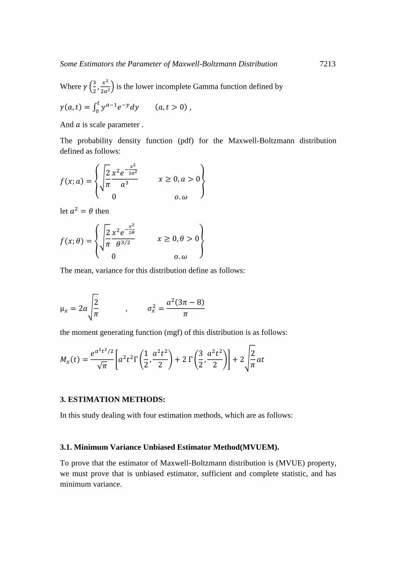
2. MAXWELL-BOLTZMANN DISTRIBUTION.
The random variable (𝑥) has Maxwell-Boltzmann distribution which contain one
parameter, it has the following cumulative distribution function (cdf):
𝐹(𝑥; 𝑎) =2
√𝜋𝛾 (
3
2,
𝑥2
2𝑎2)
Some Estimators the Parameter of Maxwell-Boltzmann Distribution 7213
Where 𝛾 (3
2,
𝑥2
2𝑎2) is the lower incomplete Gamma function defined by
𝛾(𝑎, 𝑡) = ∫ 𝑦𝑎−1𝑒−𝑦𝑑𝑦 (𝑎, 𝑡 > 0)𝑡
0 ,
And 𝑎 is scale parameter .
The probability density function (pdf) for the Maxwell-Boltzmann distribution
defined as follows:
𝑓(𝑥; 𝑎) = {√2
𝜋
𝑥2𝑒−
𝑥2
2𝑎2
𝑎3 𝑥 ≥ 0, 𝑎 > 0
0 𝑜. 𝜔
}
let 𝑎2 = 𝜃 then
𝑓(𝑥; 𝜃) = {√2
𝜋
𝑥2𝑒−𝑥2
2𝜃
𝜃3/2 𝑥 ≥ 0, 𝜃 > 0
0 𝑜. 𝜔
}
The mean, variance for this distribution define as follows:
µ𝑥 = 2𝑎√2
𝜋 , 𝜎𝑥
2 =𝑎2(3𝜋 − 8)
𝜋
the moment generating function (mgf) of this distribution is as follows:
𝑀𝑥(𝑡) =𝑒𝑎2𝑡2/2
√𝜋[𝑎2𝑡2Γ (
1
2,𝑎2𝑡2
2) + 2 Γ (
3
2,𝑎2𝑡2
2)] + 2√
2
𝜋𝑎𝑡
3. ESTIMATION METHODS:
In this study dealing with four estimation methods, which are as follows:
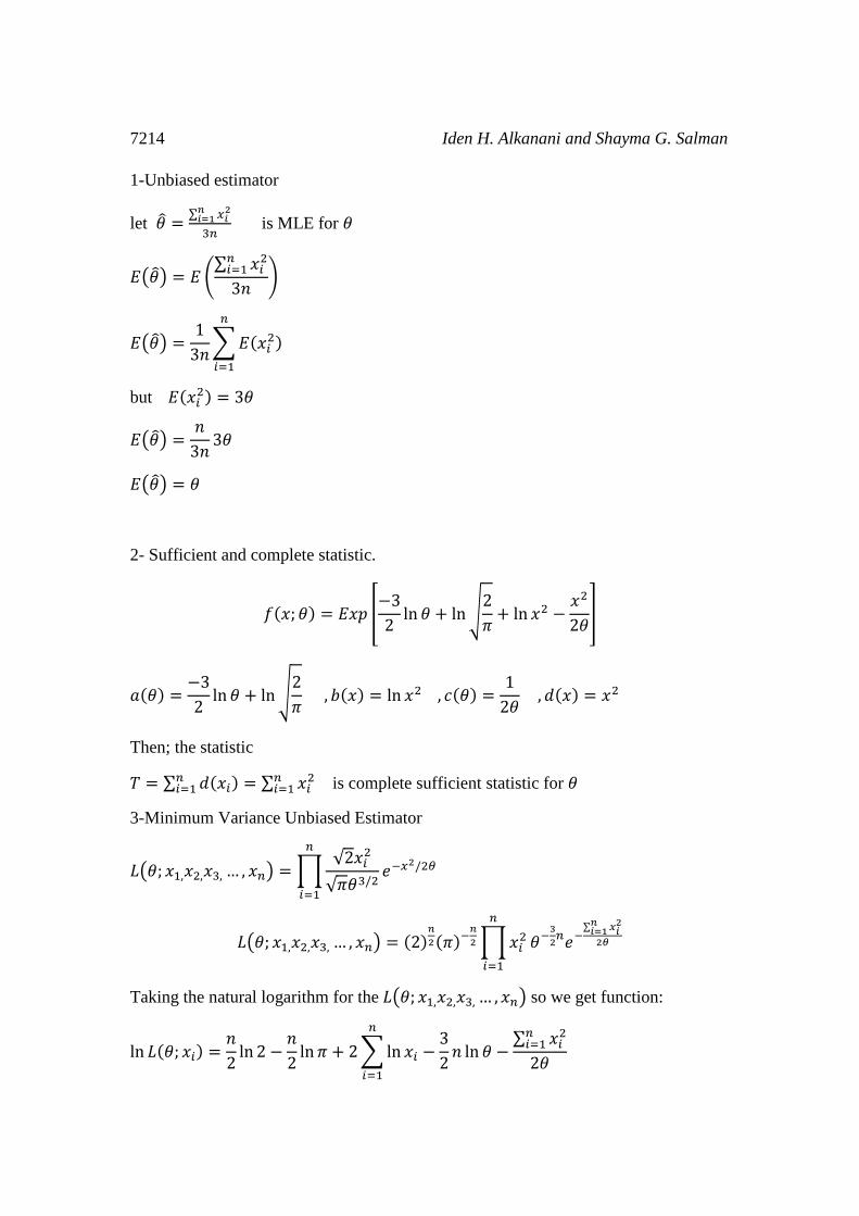
3.1. Minimum Variance Unbiased Estimator Method(MVUEM).
To prove that the estimator of Maxwell-Boltzmann distribution is (MVUE) property,
we must prove that is unbiased estimator, sufficient and complete statistic, and has
minimum variance.
7214 Iden H. Alkanani and Shayma G. Salman
1-Unbiased estimator
let 𝜃 =∑ 𝑥𝑖
2𝑛𝑖=1
3𝑛 is MLE for 𝜃
𝐸(𝜃) = 𝐸 (∑ 𝑥𝑖
2𝑛𝑖=1
3𝑛)
𝐸(𝜃) =1
3𝑛∑ 𝐸(𝑥𝑖
2)
𝑛
𝑖=1
but 𝐸(𝑥𝑖2) = 3𝜃
𝐸(𝜃) =𝑛
3𝑛3𝜃
𝐸(𝜃) = 𝜃
2- Sufficient and complete statistic.
𝑓(𝑥; 𝜃) = 𝐸𝑥𝑝 [−3
2ln 𝜃 + ln √
2
𝜋+ ln 𝑥2 −
𝑥2
2𝜃]
𝑎(𝜃) =−3
2ln 𝜃 + ln √
2
𝜋 , 𝑏(𝑥) = ln 𝑥2 , 𝑐(𝜃) =
1
2𝜃 , 𝑑(𝑥) = 𝑥2
Then; the statistic
𝑇 = ∑ 𝑑(𝑥𝑖) = ∑ 𝑥𝑖2𝑛
𝑖=1𝑛𝑖=1 is complete sufficient statistic for 𝜃
3-Minimum Variance Unbiased Estimator
𝐿(𝜃; 𝑥1,𝑥2,𝑥3, … , 𝑥𝑛) = ∏√2𝑥𝑖
2
√𝜋𝜃3/2𝑒−𝑥2/2𝜃
𝑛
𝑖=1
𝐿(𝜃; 𝑥1,𝑥2,𝑥3, … , 𝑥𝑛) = (2)𝑛
2(𝜋)−𝑛
2 ∏ 𝑥𝑖2
𝑛
𝑖=1
𝜃−3
2𝑛𝑒−
∑ 𝑥𝑖2𝑛
𝑖=12𝜃
Taking the natural logarithm for the 𝐿(𝜃; 𝑥1,𝑥2,𝑥3, … , 𝑥𝑛) so we get function:
ln 𝐿(𝜃; 𝑥𝑖) =𝑛
2ln 2 −
𝑛
2ln 𝜋 + 2 ∑ ln 𝑥𝑖 −
3
2𝑛 ln 𝜃
𝑛
𝑖=1
−∑ 𝑥𝑖
2𝑛𝑖=1
2𝜃
Some Estimators the Parameter of Maxwell-Boltzmann Distribution 7215
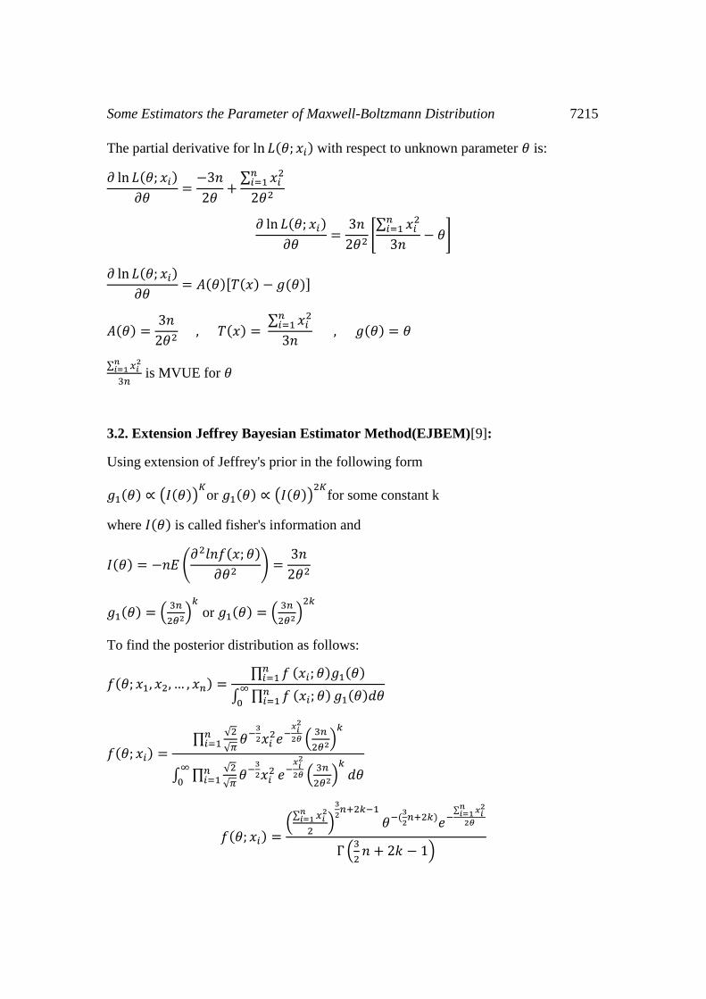
The partial derivative for ln 𝐿(𝜃; 𝑥𝑖) with respect to unknown parameter 𝜃 is:
𝜕 ln 𝐿(𝜃; 𝑥𝑖)
𝜕𝜃=
−3𝑛
2𝜃+
∑ 𝑥𝑖2𝑛
𝑖=1
2𝜃2
𝜕 ln 𝐿(𝜃; 𝑥𝑖)
𝜕𝜃=
3𝑛
2𝜃2[∑ 𝑥𝑖
2𝑛𝑖=1
3𝑛− 𝜃]
𝜕 ln 𝐿(𝜃; 𝑥𝑖)
𝜕𝜃= 𝐴(𝜃)[𝑇(𝑥) − 𝑔(𝜃)]
𝐴(𝜃) =3𝑛
2𝜃2 , 𝑇(𝑥) =
∑ 𝑥𝑖2𝑛
𝑖=1
3𝑛 , 𝑔(𝜃) = 𝜃
∑ 𝑥𝑖2𝑛
𝑖=1
3𝑛 is MVUE for 𝜃
3.2. Extension Jeffrey Bayesian Estimator Method(EJBEM)[9]:
Using extension of Jeffrey's prior in the following form
𝑔1(𝜃) ∝ (𝐼(𝜃))𝐾
or 𝑔1(𝜃) ∝ (𝐼(𝜃))2𝐾
for some constant k
where 𝐼(𝜃) is called fisher's information and
𝐼(𝜃) = −𝑛𝐸 (𝜕2𝑙𝑛𝑓(𝑥; 𝜃)
𝜕𝜃2) =
3𝑛
2𝜃2
𝑔1(𝜃) = (3𝑛
2𝜃2)𝑘
or 𝑔1(𝜃) = (3𝑛
2𝜃2)2𝑘
To find the posterior distribution as follows:
𝑓(𝜃; 𝑥1, 𝑥2, … , 𝑥𝑛) =∏ 𝑓𝑛
𝑖=1 (𝑥𝑖; 𝜃)𝑔1(𝜃)
∫ ∏ 𝑓𝑛𝑖=1 (𝑥𝑖; 𝜃)
∞
0𝑔1(𝜃)𝑑𝜃
𝑓(𝜃; 𝑥𝑖) =∏
√2
√𝜋
𝑛𝑖=1 𝜃−
3
2𝑥𝑖2𝑒−
𝑥𝑖2
2𝜃 (3𝑛
2𝜃2)𝑘
∫ ∏√2
√𝜋𝑛𝑖=1 𝜃−
3
2𝑥𝑖2∞
0𝑒−
𝑥𝑖2
2𝜃 (3𝑛
2𝜃2)
𝑘
𝑑𝜃
𝑓(𝜃; 𝑥𝑖) =(
∑ 𝑥𝑖2𝑛
𝑖=1
2)
3
2𝑛+2𝑘−1
𝜃−(3
2𝑛+2𝑘)𝑒−
∑ 𝑥𝑖2𝑛
𝑖=12𝜃
Г (3
2𝑛 + 2𝑘 − 1)
7216 Iden H. Alkanani and Shayma G. Salman
by using squared error loss function 𝐿(𝜃, 𝜃) = (𝜃 − 𝜃)2, the risk function is:
𝑅(𝜃) = ∫ 𝐿(𝜃, 𝜃)𝑓(𝜃; 𝑥𝑖)𝑑𝜃∞
0
𝑅(𝜃) = ∫ (𝜃 − 𝜃)2 (
∑ 𝑥𝑖2𝑛
𝑖=1
2)
3
2𝑛+2𝑘−1
𝜃−(3
2𝑛+2𝑘)𝑒−
∑ 𝑥𝑖2𝑛
𝑖=12𝜃
Г (3
2𝑛 + 2𝑘 − 1)
𝑑𝜃∞
0
𝑅(𝜃) = 𝜃2 −𝜃 ∑ 𝑥𝑖
2𝑛𝑖=1
(3
2𝑛 + 2𝑘 − 2 )
+ ℎ
The partial derivative for 𝑅(𝜃) with respect to 𝜃 we get
𝜕𝑅(𝜃)
𝜕𝜃= 2𝜃 −
∑ 𝑥𝑖2𝑛
𝑖=13
2𝑛 + 2𝑘 − 2
+ 𝑧𝑒𝑟𝑜
the Bayes estimator 𝜃 is the solution of equation 𝜕𝑅(𝜃)
𝜕�̂�= 0, which results in
𝜃 =∑ 𝑥𝑖
2𝑛𝑖=1
3𝑛+4𝑘−4 is EJBE for 𝜃
3.3. Informative Bayesian prior Estimator method(IBEM):
We based on Improper(𝑎, 𝑏) distribution as informative prior to derive the posterior
distribution, which is as follows:
𝑔2(𝜃) = {𝜃−(𝑎+1)𝑒−(𝑏
𝜃), 𝜃 > 0, −∞ < 𝑎 < ∞
0 , 𝑜. 𝑤 , 𝑏 > 0
To find the posterior distribution of 𝜃 as follows
𝑓(𝜃; 𝑥1, 𝑥2, … , 𝑥𝑛) =∏ 𝑓𝑛
𝑖=1 (𝑥𝑖; 𝜃)𝑔2(𝜃)
∫ ∏ 𝑓𝑛𝑖=1 (𝑥𝑖; 𝜃)
∞
0𝑔2(𝜃)𝑑𝜃
𝑓(𝜃; 𝑥𝑖) =(
√2
√𝜋)
𝑛
𝜃−3
2𝑛 ∏ 𝑥𝑖
2𝑛𝑖=1 𝑒−
∑ 𝑥𝑖2𝑛
𝑖=12𝜃 𝜃−(𝑎+1)𝑒−(
𝑏
𝜃)
∫ (√2
√𝜋)
𝑛
𝜃−3
2𝑛 ∏ 𝑥𝑖
2𝑛𝑖=1
∞
0𝑒−
∑ 𝑥𝑖2𝑛
𝑖=12𝜃 𝜃−(𝑎+1)𝑒−(
𝑏
𝜃)𝑑𝜃
Some Estimators the Parameter of Maxwell-Boltzmann Distribution 7217
𝑓(𝜃; 𝑥𝑖) =(
∑ 𝑥𝑖2𝑛
𝑖=1 +2𝑏
2)
3
2𝑛+𝑎
𝜃−(3
2𝑛+𝑎+1)𝑒−
(∑ 𝑥𝑖2𝑛
𝑖=1 +2𝑏)
2𝜃
Г (3
2𝑛 + 𝑎)
By using squared error loss function 𝐿(𝜃, 𝜃) = (𝜃 − 𝜃)2,the risk function is:
𝑅(𝜃) = ∫ 𝐿(𝜃, 𝜃)𝑓(𝜃; 𝑥𝑖)𝑑𝜃∞
0
𝑅(𝜃) = ∫ (𝜃 − 𝜃)2 (
∑ 𝑥𝑖2𝑛
𝑖=1 +2𝑏
2)
3
2𝑛+𝑎
𝜃−(3
2𝑛+𝑎+1)𝑒−
(∑ 𝑥𝑖2𝑛
𝑖=1 +2𝑏)
2𝜃
Г (3
2𝑛 + 𝑎)
𝑑𝜃∞
0
𝑅(𝜃) = 𝜃2 −𝜃(∑ 𝑥𝑖
2𝑛𝑖=1 + 2𝑏)
(3
2𝑛 + 𝑎 − 1)
+ 𝑘
The partial derivative for 𝑅(𝜃) with respect to 𝜃 we get
𝜕𝑅(𝜃)
𝜕𝜃= 2𝜃 −
∑ 𝑥𝑖2𝑛
𝑖=1 + 2𝑏3
2𝑛 + 𝑎 − 1
+ 𝑧𝑒𝑟𝑜
the Bayes estimator 𝜃 is the solution of equation 𝜕𝑅(𝜃)
𝜕�̂�= 0, which results in
2𝜃 −∑ 𝑥𝑖
2𝑛𝑖=1 + 2𝑏
3
2𝑛 + 𝑎 − 1
= 0
𝜃 =∑ 𝑥𝑖
2𝑛𝑖=1 +2𝑏
3𝑛+2𝑎−2 is IBE for 𝜃
3.4. Shrinkage Estimator Method(SEM)[10]:
In many problems there is some prior information about the parameter 𝜃 and this prior
information is created as initial values symbolled by 𝜃0,Then the estimated method
for this case is called Shrinkage estimation method.
The Shrinkage estimator is a linear combination between initial value 𝜃0 and
estimated value 𝜃 based on Shrinkage weight function which is denoted by 𝜓(𝜃).
There are two types of Shrinkage weight function which are as follows:
7218 Iden H. Alkanani and Shayma G. Salman
a-Constant Shrinkage weight function K:
The Shrinkage estimation of 𝜃 is:
�̃� = 𝐾𝜃 + (1 − 𝐾)𝜃0
where K is constant, 𝐾 ∈ [0,1], K is confidence quantity for 𝜃 and (1 − 𝐾) is
confidence quantity for 𝜃0.
b-Variable Shrinkage weight function 𝜓(𝜃):
The Shrinkage estimation of 𝜃 is :
�̃� = 𝜓(𝜃)𝜃 + [1 − 𝜓(𝜃)]𝜃0
where 𝜓(𝜃) is Shrinkage weight function depend on 𝜃, 𝜓(𝜃) ∈ [0,1],
and 𝜓(𝜃) is a confidence quantity for𝜃,[1 − 𝜓(𝜃)] is a confidence quantity for 𝜃0.
Now, for Maxwell-Boltzmann distribution, we can find the Shrinkage estimator for
the scale parameter 𝜃 as follows:
�̃� = 𝜓(𝜃)𝜃 + [1 − 𝜓(𝜃)]𝜃0
𝜓(𝜃) =𝑏
10𝑣𝑎𝑟(𝜃)
𝜃 is MLE of 𝜃,𝜃0 is initial value which is prior information, 𝑏 is any constant and
0˂𝑏 ≤ 1, 𝑣𝑎𝑟(𝜃) get it from fisher information matrix for MLE method.
The Shrinkage estimator for 𝜃 is became as following.
�̃� =𝑏
10𝑣𝑎𝑟(𝜃)𝜃 + [1 −
𝑏
10𝑣𝑎𝑟(𝜃)] 𝜃0
the mean square error for Shrinkage estimator for 𝜃 is as follows
𝑀𝑆𝐸(�̃�) = 𝐸(�̃� − 𝜃)2
𝑀𝑆𝐸(�̃�) = 𝐸 [𝑏
10𝑣𝑎𝑟(𝜃)𝜃 + (1 −
𝑏
10𝑣𝑎𝑟(𝜃)) 𝜃0 − 𝜃]
2
𝑀𝑆𝐸(�̃�) =𝑏2
100𝑣𝑎𝑟2(𝜃)𝐸(𝜃 − 𝜃0)
2−
2𝑏
10𝑣𝑎𝑟(𝜃)(𝜃 − 𝜃0)𝐸(𝜃 − 𝜃0) + (𝜃 − 𝜃0)2
to get the value of 𝑏 we must minimize the mean square error then
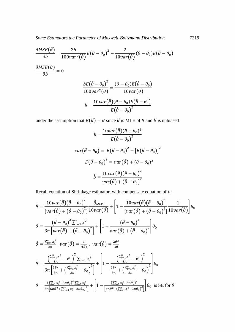
Some Estimators the Parameter of Maxwell-Boltzmann Distribution 7219
𝜕𝑀𝑆𝐸(�̃�)
𝜕𝑏=
2𝑏
100𝑣𝑎𝑟2(𝜃)𝐸(𝜃 − 𝜃0)
2−
2
10𝑣𝑎𝑟(𝜃)(𝜃 − 𝜃0)𝐸(𝜃 − 𝜃0)
𝜕𝑀𝑆𝐸(�̃�)
𝜕𝑏= 0
𝑏𝐸(𝜃 − 𝜃0)2
100𝑣𝑎𝑟2(𝜃)=
(𝜃 − 𝜃0)𝐸(𝜃 − 𝜃0)
10𝑣𝑎𝑟(𝜃)
𝑏 =10𝑣𝑎𝑟(𝜃)(𝜃 − 𝜃0)𝐸(𝜃 − 𝜃0)
𝐸(𝜃 − 𝜃0)2
under the assumption that 𝐸(𝜃) = 𝜃 since 𝜃 is MLE of 𝜃 and 𝜃 is unbiased
𝑏 =10𝑣𝑎𝑟(𝜃)(𝜃 − 𝜃0)2
𝐸(𝜃 − 𝜃0)2
𝑣𝑎𝑟(𝜃 − 𝜃0) = 𝐸(𝜃 − 𝜃0)2
− [𝐸(𝜃 − 𝜃0)]2
𝐸(𝜃 − 𝜃0)2
= 𝑣𝑎𝑟(𝜃) + (𝜃 − 𝜃0)2
�̂� =10𝑣𝑎𝑟(𝜃)(𝜃 − 𝜃0)
2
𝑣𝑎𝑟(𝜃) + (𝜃 − 𝜃0)2
Recall equation of Shrinkage estimator, with compensate equation of 𝑏:
�̃� =10𝑣𝑎𝑟(𝜃)(𝜃 − 𝜃0)
2
[𝑣𝑎𝑟(𝜃) + (𝜃 − 𝜃0)2
]
𝜃𝑀𝐿𝐸
10𝑣𝑎𝑟(𝜃)+ [1 −
10𝑣𝑎𝑟(𝜃)(𝜃 − 𝜃0)2
[𝑣𝑎𝑟(𝜃) + (𝜃 − 𝜃0)2
]
1
10𝑣𝑎𝑟(𝜃)] 𝜃0
�̃� =(𝜃 − 𝜃0)
2∑ 𝑥𝑖
2𝑛𝑖=1
3𝑛 [𝑣𝑎𝑟(𝜃) + (𝜃 − 𝜃0)2
]+ [1 −
(𝜃 − 𝜃0)2
𝑣𝑎𝑟(𝜃) + (𝜃 − 𝜃0)2] 𝜃0
𝜃 =∑ 𝑥𝑖
2𝑛𝑖=1
3𝑛 , 𝑣𝑎𝑟(𝜃) =
1
𝐼(𝜃) , 𝑣𝑎𝑟(𝜃) =
2𝜃2
3𝑛
�̃� =(
∑ 𝑥𝑖2𝑛
𝑖=1
3𝑛− 𝜃0)
2
∑ 𝑥𝑖2𝑛
𝑖=1
3𝑛 [2𝜃2
3𝑛+ (
∑ 𝑥𝑖2𝑛
𝑖=1
3𝑛− 𝜃0)
2
]
+ [1 −(
∑ 𝑥𝑖2𝑛
𝑖=1
3𝑛− 𝜃0)
2
2𝜃2
3𝑛+ (
∑ 𝑥𝑖2𝑛
𝑖=1
3𝑛− 𝜃0)
2] 𝜃0
�̃� =(∑ 𝑥𝑖
2−3𝑛𝜃0𝑛𝑖=1 )
2∑ 𝑥𝑖
2𝑛𝑖=1
3𝑛[6𝑛𝜃2+(∑ 𝑥𝑖2−3𝑛𝜃0
𝑛𝑖=1 )
2]
+ [1 −(∑ 𝑥𝑖
2−3𝑛𝜃0𝑛𝑖=1 )
2
[6𝑛𝜃2+(∑ 𝑥𝑖2−3𝑛𝜃0
𝑛𝑖=1 )
2]] 𝜃0 is SE for 𝜃
7220 Iden H. Alkanani and Shayma G. Salman
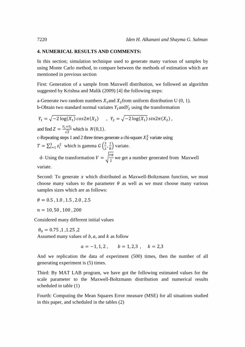
4. NUMERICAL RESULTS AND COMMENTS:
In this section; simulation technique used to generate many various of samples by
using Monte Carlo method, to compare between the methods of estimation which are
mentioned in previous section
First: Generation of a sample from Maxwell distribution, we followed an algorithm
suggested by Krishna and Malik (2009) [4] the following steps:
a-Generate two random numbers 𝑋1and 𝑋2from uniform distribution U (0, 1).
b-Obtain two standard normal variates 𝑌1and𝑌2 using the transformation
𝑌1 = √−2 log(𝑋1) 𝑐𝑜𝑠2𝜋(𝑋2) , 𝑌2 = √−2 log(𝑋1) 𝑠𝑖𝑛2𝜋(𝑋2) ,
and find 𝑍 =𝑌1+𝑌2
√2 which is 𝑁(0,1).
c-Repeating steps 1 and 2 three times generate a chi-square 𝑋32 variate using
𝑇 = ∑ 𝑧𝑖23
𝑖=1 which is gamma 𝐺 (3
2,
1
𝜃) variate.
we get a number generated from Maxwell 𝑉 = √𝑇𝜃
2 Using the transformation -d
variate.
Second: To generate 𝑥 which distributed as Maxwell-Boltzmann function, we must
choose many values to the parameter 𝜃 as well as we must choose many various
samples sizes which are as follows:
𝜃 = 0.5 , 1.0 , 1.5 , 2.0 , 2.5
𝑛 = 10, 50 , 100 , 200
Considered many different initial values
𝜃0 = 0.75 ,1 ,1.25 ,2
Assumed many values of 𝑏, 𝑎, and 𝑘 as follow
𝑎 = −1, 1, 2 , 𝑏 = 1, 2,3 , 𝑘 = 2,3
And we replication the data of experiment (500) times, then the number of all
generating experiment is (5) times.
Third: By MAT LAB program, we have got the following estimated values for the
scale parameter to the Maxwell-Boltzmann distribution and numerical results
scheduled in table (1)
Fourth: Computing the Mean Squares Error measure (MSE) for all situations studied
in this paper, and scheduled in the tables (2)
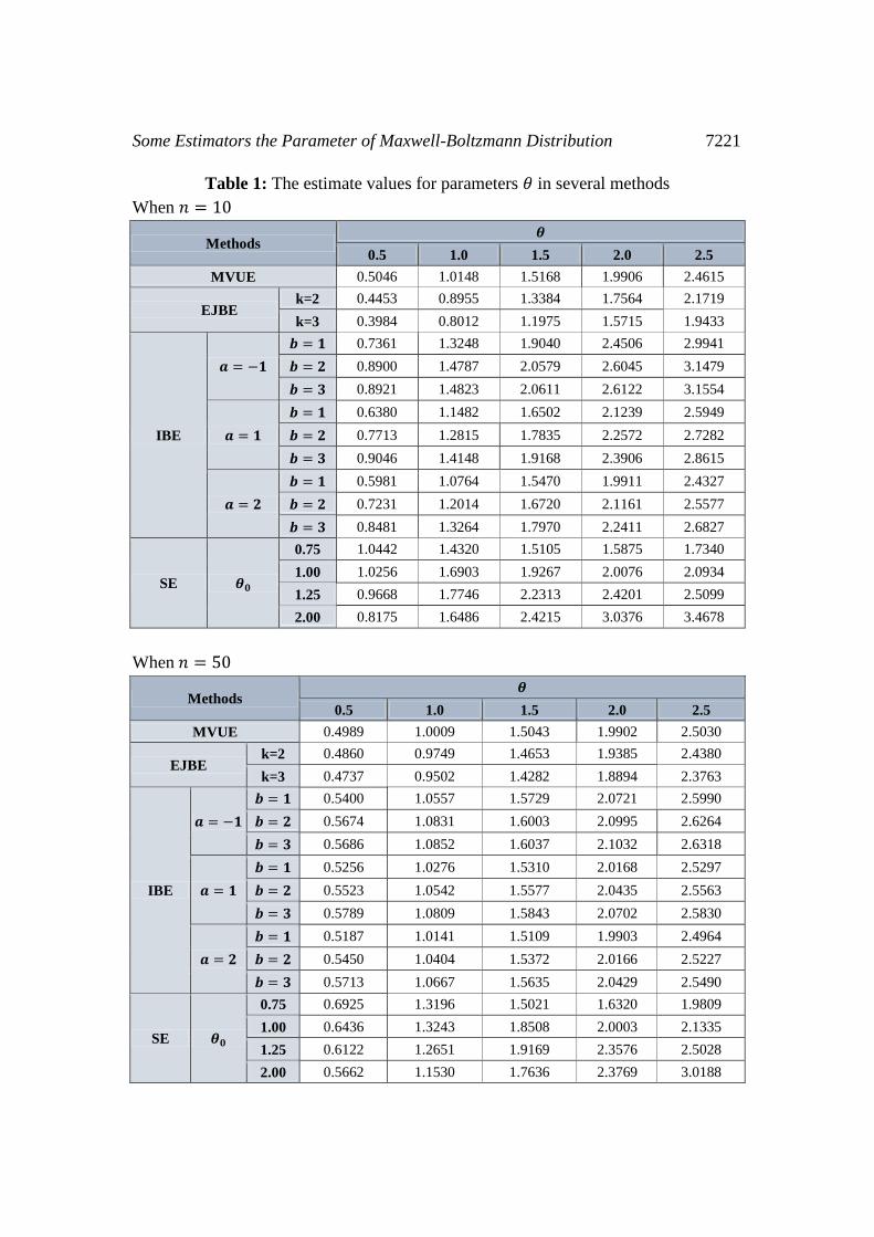
Some Estimators the Parameter of Maxwell-Boltzmann Distribution 7221
Table 1: The estimate values for parameters 𝜃 in several methods
When 𝑛 = 10
Methods 𝜽
0.5 1.0 1.5 2.0 2.5
MVUE 0.5046 1.0148 1.5168 1.9906 2.4615
EJBE k=2 0.4453 0.8955 1.3384 1.7564 2.1719
k=3 0.3984 0.8012 1.1975 1.5715 1.9433
IBE
𝒂 = −𝟏
𝒃 = 𝟏 0.7361 1.3248 1.9040 2.4506 2.9941
𝒃 = 𝟐 0.8900 1.4787 2.0579 2.6045 3.1479
𝒃 = 𝟑 0.8921 1.4823 2.0611 2.6122 3.1554
𝒂 = 𝟏
𝒃 = 𝟏 0.6380 1.1482 1.6502 2.1239 2.5949
𝒃 = 𝟐 0.7713 1.2815 1.7835 2.2572 2.7282
𝒃 = 𝟑 0.9046 1.4148 1.9168 2.3906 2.8615
𝒂 = 𝟐
𝒃 = 𝟏 0.5981 1.0764 1.5470 1.9911 2.4327
𝒃 = 𝟐 0.7231 1.2014 1.6720 2.1161 2.5577
𝒃 = 𝟑 0.8481 1.3264 1.7970 2.2411 2.6827
SE 𝜽𝟎
0.75 1.0442 1.4320 1.5105 1.5875 1.7340
1.00 1.0256 1.6903 1.9267 2.0076 2.0934
1.25 0.9668 1.7746 2.2313 2.4201 2.5099
2.00 0.8175 1.6486 2.4215 3.0376 3.4678
When 𝑛 = 50
Methods 𝜽
0.5 1.0 1.5 2.0 2.5
MVUE 0.4989 1.0009 1.5043 1.9902 2.5030
EJBE k=2 0.4860 0.9749 1.4653 1.9385 2.4380
k=3 0.4737 0.9502 1.4282 1.8894 2.3763
IBE
𝒂 = −𝟏
𝒃 = 𝟏 0.5400 1.0557 1.5729 2.0721 2.5990
𝒃 = 𝟐 0.5674 1.0831 1.6003 2.0995 2.6264
𝒃 = 𝟑 0.5686 1.0852 1.6037 2.1032 2.6318
𝒂 = 𝟏
𝒃 = 𝟏 0.5256 1.0276 1.5310 2.0168 2.5297
𝒃 = 𝟐 0.5523 1.0542 1.5577 2.0435 2.5563
𝒃 = 𝟑 0.5789 1.0809 1.5843 2.0702 2.5830
𝒂 = 𝟐
𝒃 = 𝟏 0.5187 1.0141 1.5109 1.9903 2.4964
𝒃 = 𝟐 0.5450 1.0404 1.5372 2.0166 2.5227
𝒃 = 𝟑 0.5713 1.0667 1.5635 2.0429 2.5490
SE 𝜽𝟎
0.75 0.6925 1.3196 1.5021 1.6320 1.9809
1.00 0.6436 1.3243 1.8508 2.0003 2.1335
1.25 0.6122 1.2651 1.9169 2.3576 2.5028
2.00 0.5662 1.1530 1.7636 2.3769 3.0188
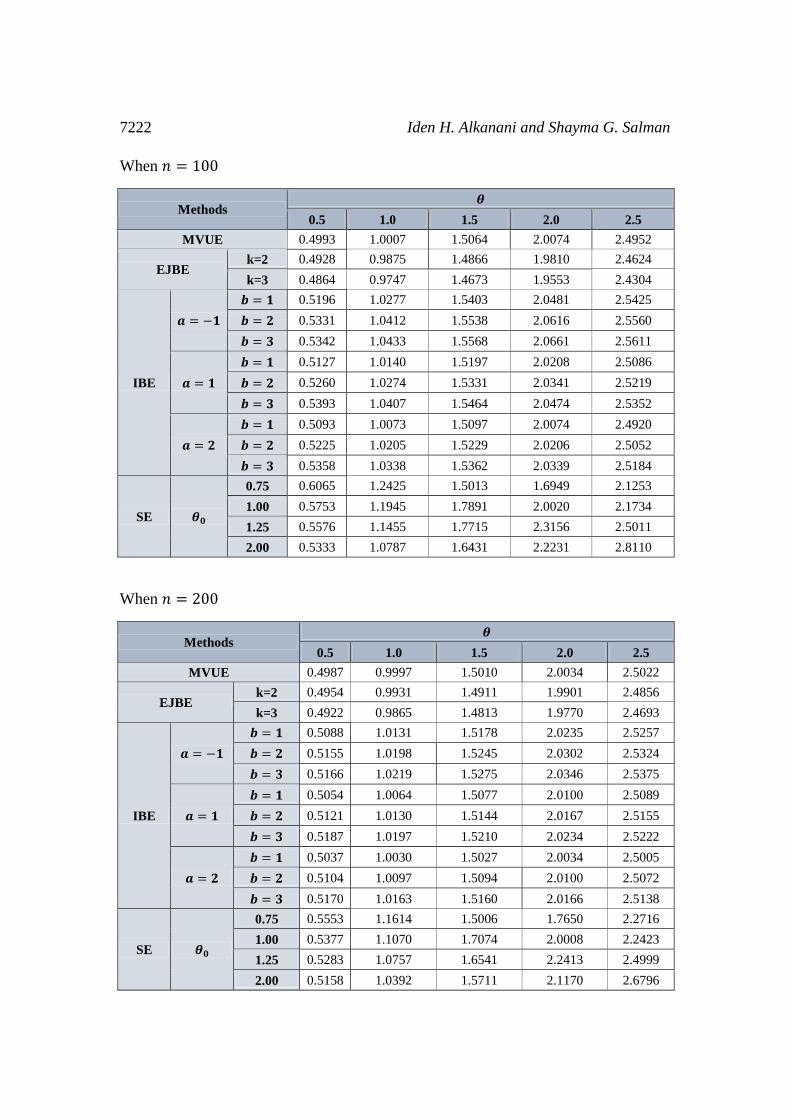
7222 Iden H. Alkanani and Shayma G. Salman
When 𝑛 = 100
Methods 𝜽
0.5 1.0 1.5 2.0 2.5
MVUE 0.4993 1.0007 1.5064 2.0074 2.4952
EJBE k=2 0.4928 0.9875 1.4866 1.9810 2.4624
k=3 0.4864 0.9747 1.4673 1.9553 2.4304
IBE
𝒂 = −𝟏
𝒃 = 𝟏 0.5196 1.0277 1.5403 2.0481 2.5425
𝒃 = 𝟐 0.5331 1.0412 1.5538 2.0616 2.5560
𝒃 = 𝟑 0.5342 1.0433 1.5568 2.0661 2.5611
𝒂 = 𝟏
𝒃 = 𝟏 0.5127 1.0140 1.5197 2.0208 2.5086
𝒃 = 𝟐 0.5260 1.0274 1.5331 2.0341 2.5219
𝒃 = 𝟑 0.5393 1.0407 1.5464 2.0474 2.5352
𝒂 = 𝟐
𝒃 = 𝟏 0.5093 1.0073 1.5097 2.0074 2.4920
𝒃 = 𝟐 0.5225 1.0205 1.5229 2.0206 2.5052
𝒃 = 𝟑 0.5358 1.0338 1.5362 2.0339 2.5184
SE 𝜽𝟎
0.75 0.6065 1.2425 1.5013 1.6949 2.1253
1.00 0.5753 1.1945 1.7891 2.0020 2.1734
1.25 0.5576 1.1455 1.7715 2.3156 2.5011
2.00 0.5333 1.0787 1.6431 2.2231 2.8110
When 𝑛 = 200
Methods 𝜽
0.5 1.0 1.5 2.0 2.5
MVUE 0.4987 0.9997 1.5010 2.0034 2.5022
EJBE k=2 0.4954 0.9931 1.4911 1.9901 2.4856
k=3 0.4922 0.9865 1.4813 1.9770 2.4693
IBE
𝒂 = −𝟏
𝒃 = 𝟏 0.5088 1.0131 1.5178 2.0235 2.5257
𝒃 = 𝟐 0.5155 1.0198 1.5245 2.0302 2.5324
𝒃 = 𝟑 0.5166 1.0219 1.5275 2.0346 2.5375
𝒂 = 𝟏
𝒃 = 𝟏 0.5054 1.0064 1.5077 2.0100 2.5089
𝒃 = 𝟐 0.5121 1.0130 1.5144 2.0167 2.5155
𝒃 = 𝟑 0.5187 1.0197 1.5210 2.0234 2.5222
𝒂 = 𝟐
𝒃 = 𝟏 0.5037 1.0030 1.5027 2.0034 2.5005
𝒃 = 𝟐 0.5104 1.0097 1.5094 2.0100 2.5072
𝒃 = 𝟑 0.5170 1.0163 1.5160 2.0166 2.5138
SE 𝜽𝟎
0.75 0.5553 1.1614 1.5006 1.7650 2.2716
1.00 0.5377 1.1070 1.7074 2.0008 2.2423
1.25 0.5283 1.0757 1.6541 2.2413 2.4999
2.00 0.5158 1.0392 1.5711 2.1170 2.6796
Some Estimators the Parameter of Maxwell-Boltzmann Distribution 7223
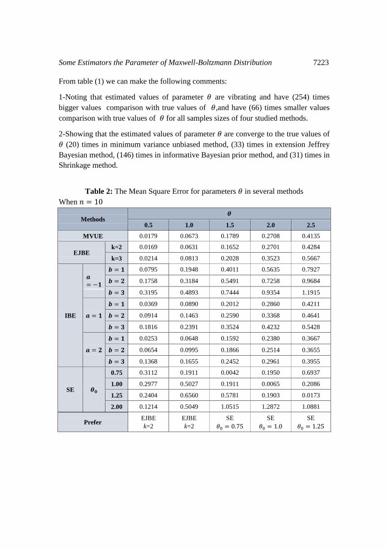
From table (1) we can make the following comments:
1-Noting that estimated values of parameter 𝜃 are vibrating and have (254) times
bigger values comparison with true values of 𝜃,and have (66) times smaller values
comparison with true values of 𝜃 for all samples sizes of four studied methods.
2-Showing that the estimated values of parameter 𝜃 are converge to the true values of
𝜃 (20) times in minimum variance unbiased method, (33) times in extension Jeffrey
Bayesian method, (146) times in informative Bayesian prior method, and (31) times in
Shrinkage method.
Table 2: The Mean Square Error for parameters 𝜃 in several methods
When 𝑛 = 10
Methods 𝜽
0.5 1.0 1.5 2.0 2.5
MVUE 0.0179 0.0673 0.1789 0.2708 0.4135
EJBE k=2 0.0169 0.0631 0.1652 0.2701 0.4284
k=3 0.0214 0.0813 0.2028 0.3523 0.5667
IBE
𝒂= −𝟏
𝒃 = 𝟏 0.0795 0.1948 0.4011 0.5635 0.7927
𝒃 = 𝟐 0.1758 0.3184 0.5491 0.7258 0.9684
𝒃 = 𝟑 0.3195 0.4893 0.7444 0.9354 1.1915
𝒂 = 𝟏
𝒃 = 𝟏 0.0369 0.0890 0.2012 0.2860 0.4211
𝒃 = 𝟐 0.0914 0.1463 0.2590 0.3368 0.4641
𝒃 = 𝟑 0.1816 0.2391 0.3524 0.4232 0.5428
𝒂 = 𝟐
𝒃 = 𝟏 0.0253 0.0648 0.1592 0.2380 0.3667
𝒃 = 𝟐 0.0654 0.0995 0.1866 0.2514 0.3655
𝒃 = 𝟑 0.1368 0.1655 0.2452 0.2961 0.3955
SE 𝜽𝟎
0.75 0.3112 0.1911 0.0042 0.1950 0.6937
1.00 0.2977 0.5027 0.1911 0.0065 0.2086
1.25 0.2404 0.6560 0.5781 0.1903 0.0173
2.00 0.1214 0.5049 1.0515 1.2872 1.0881
Prefer EJBE
k=2
EJBE
k=2
SE
𝜃0 = 0.75
SE
𝜃0 = 1.0
SE
𝜃0 = 1.25
7224 Iden H. Alkanani and Shayma G. Salman
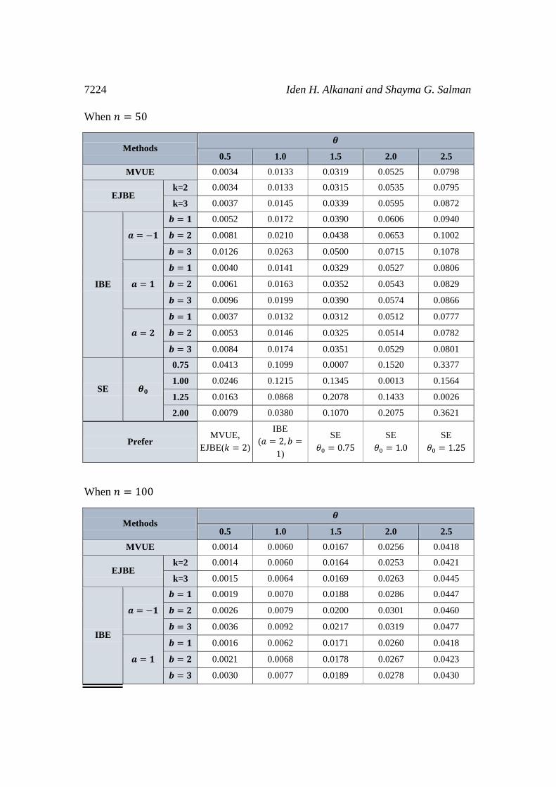
When 𝑛 = 50
Methods 𝜽
0.5 1.0 1.5 2.0 2.5
MVUE 0.0034 0.0133 0.0319 0.0525 0.0798
EJBE k=2 0.0034 0.0133 0.0315 0.0535 0.0795
k=3 0.0037 0.0145 0.0339 0.0595 0.0872
IBE
𝒂 = −𝟏
𝒃 = 𝟏 0.0052 0.0172 0.0390 0.0606 0.0940
𝒃 = 𝟐 0.0081 0.0210 0.0438 0.0653 0.1002
𝒃 = 𝟑 0.0126 0.0263 0.0500 0.0715 0.1078
𝒂 = 𝟏
𝒃 = 𝟏 0.0040 0.0141 0.0329 0.0527 0.0806
𝒃 = 𝟐 0.0061 0.0163 0.0352 0.0543 0.0829
𝒃 = 𝟑 0.0096 0.0199 0.0390 0.0574 0.0866
𝒂 = 𝟐
𝒃 = 𝟏 0.0037 0.0132 0.0312 0.0512 0.0777
𝒃 = 𝟐 0.0053 0.0146 0.0325 0.0514 0.0782
𝒃 = 𝟑 0.0084 0.0174 0.0351 0.0529 0.0801
SE 𝜽𝟎
0.75 0.0413 0.1099 0.0007 0.1520 0.3377
1.00 0.0246 0.1215 0.1345 0.0013 0.1564
1.25 0.0163 0.0868 0.2078 0.1433 0.0026
2.00 0.0079 0.0380 0.1070 0.2075 0.3621
Prefer MVUE,
EJBE(𝑘 = 2)
IBE
(𝑎 = 2, 𝑏 =
1)
SE
𝜃0 = 0.75
SE
𝜃0 = 1.0
SE
𝜃0 = 1.25
When 𝑛 = 100
Methods 𝜽
0.5 1.0 1.5 2.0 2.5
MVUE 0.0014 0.0060 0.0167 0.0256 0.0418
EJBE k=2 0.0014 0.0060 0.0164 0.0253 0.0421
k=3 0.0015 0.0064 0.0169 0.0263 0.0445
IBE
𝒂 = −𝟏
𝒃 = 𝟏 0.0019 0.0070 0.0188 0.0286 0.0447
𝒃 = 𝟐 0.0026 0.0079 0.0200 0.0301 0.0460
𝒃 = 𝟑 0.0036 0.0092 0.0217 0.0319 0.0477
𝒂 = 𝟏
𝒃 = 𝟏 0.0016 0.0062 0.0171 0.0260 0.0418
𝒃 = 𝟐 0.0021 0.0068 0.0178 0.0267 0.0423
𝒃 = 𝟑 0.0030 0.0077 0.0189 0.0278 0.0430
Some Estimators the Parameter of Maxwell-Boltzmann Distribution 7225
𝒂 = 𝟐
𝒃 = 𝟏 0.0015 0.0060 0.0166 0.0253 0.0413
𝒃 = 𝟐 0.0019 0.0064 0.0170 0.0257 0.0413
𝒃 = 𝟑 0.0027 0.0071 0.0178 0.0264 0.0416
SE 𝜽𝟎
0.75 0.0130 0.0646 0.0004 0.1091 0.1887
1.00 0.0072 0.0454 0.0953 0.0008 0.1275
1.25 0.0048 0.0282 0.0945 0.1135 0.0013
2.00 0.0026 0.0125 0.0389 0.0799 0.1490
Prefer
MVUE,
EJBE(k=2)
MVU
EJB(k=2)
IBE
𝑎 = 2, 𝑏 = 1
SE
𝜃0 = 0.75
SE
𝜃0 = 1.0
SE
𝜃0 = 1.25
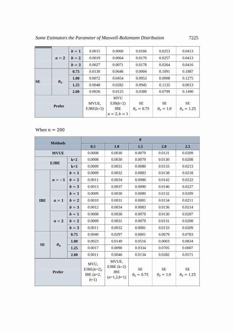
When 𝑛 = 200
Methods 𝜽
0.5 1.0 1.5 2.0 2.5
MVUE 0.0008 0.0030 0.0079 0.0131 0.0209
EJBE k=2 0.0008 0.0030 0.0079 0.0130 0.0208
k=3 0.0009 0.0031 0.0080 0.0133 0.0213
IBE
𝒂 = −𝟏
𝒃 = 𝟏 0.0009 0.0032 0.0083 0.0138 0.0218
𝒃 = 𝟐 0.0011 0.0034 0.0086 0.0142 0.0222
𝒃 = 𝟑 0.0013 0.0037 0.0090 0.0146 0.0227
𝒂 = 𝟏
𝒃 = 𝟏 0.0009 0.0030 0.0080 0.0132 0.0209
𝒃 = 𝟐 0.0010 0.0031 0.0081 0.0134 0.0211
𝒃 = 𝟑 0.0012 0.0034 0.0083 0.0136 0.0214
𝒂 = 𝟐
𝒃 = 𝟏 0.0008 0.0030 0.0079 0.0130 0.0207
𝒃 = 𝟐 0.0009 0.0031 0.0079 0.0131 0.0208
𝒃 = 𝟑 0.0011 0.0032 0.0081 0.0133 0.0209
SE 𝜽𝟎
0.75 0.0040 0.0297 0.0001 0.0679 0.0783
1.00 0.0023 0.0149 0.0516 0.0003 0.0834
1.25 0.0017 0.0090 0.0334 0.0705 0.0007
2.00 0.0011 0.0046 0.0134 0.0282 0.0571
Prefer
MVU,
EJBE(k=2),
IBE (a=2,
b=1)
MVUE,
EJBE (k=2)
IBE
(a=1,2,b=1)
SE
𝜃0 = 0.75
SE
𝜃0 = 1.0
SE
𝜃0 = 1.25
7226 Iden H. Alkanani and Shayma G. Salman
From table (2) we can make the following comments:
1-The values of mean squares error for 𝜃 are decreasing where the samples sizes are
increasing for all values of 𝜃 in all methods.
2-Noting that the values of MSE are vibrating for all increasing value of 𝜃. The
smallest values of MSE are (0.0001) when (𝜃 = 1.5 , 𝑛 = 200) for Shrinkage
estimator method at 𝜃0 = 0.75.
5. CONCLUSIONS:
Throughout the estimator parameters for all four methods, we see that all values of
estimator parameters are close to the true values of parameters in Maxwell-Boltzmann
distribution. Also we can see that the mean squared error procedure for all four
methods have a smallest value, specially the Shrinkage estimator method and far
away from informative Bayesian prior estimator method.
REFERENCES:
[1] Tyagi, R.K. and Bhattacharya, S.K. (1989), " Bayes estimation of the
Maxwell's velocity distribution function",Statistica, 29(4): 563-567.
[2] Chaturvedi, A. and Rani, U. (1998), "Classical and Bayesian Reliability
estimation of the generalized Maxwell failure distribution", J. of Stat. Res., 32,
113-120.
[3] Bekker, A. and Roux, J.J. (2005): Reliability characteristics of the Maxwell
distribution: A Bayes estimation study. Comm. Stat. (Theory & Math.),
34(11): 2169 - 2178.
[4] Krishna, H and Malik, M. (2009), " Reliability estimation in Maxwell
distribution with Type-II censored data", Int. Journal of Quality and
Reliability management, 26 (2): 184 – 195.
[5] Kasmi, A. S. M., Aslam, M., and Ali, S. (2011), "A note of Maximum
likelihood estimator for the mixture of Maxwell distributions using Type-I
censored scheme", The open stat. and prob. Journal, (3): 31 – 35.
[6] Ali Kasmi, S.M., Aslam, M., and Ali, S. (2012), " on the Bayesian estimation
for two component mixture of Maxwell distribution, assuming type I censored
data", Int. J. of Applied Science and Technology: 2(1): 197- 218.
[7] Al-Baldawi, T.H.K, (2013), "Comparison of Maximum Likelihood and some
Bayes Estimators for Maxwell Distribution based on Non-Informative Priors",
Baghdad Science JournalVol.10(2), pp 480-488.
[8] Rasheed, H. A. and Khalifa, Z.N, (2016), "Bayes Estimators For The Maxwell
Some Estimators the Parameter of Maxwell-Boltzmann Distribution 7227
Distribution Under Quadratic Loss Function Using Different Priors ",
Australian Journal of Basic and Applied Sciences, Vol.10(6), pp 97-103.
[9] Sanku, D. and Tanujit, D.,(2011), " Rayleigh Distribution Revisited VIA
Extension of Jeffrey's prior Information and a New Loss Function", statistical
journal, Vol.9, N.3, PP 214-226.
[10] Handa N.S, K.A.M.O., Brnal-Hemyari, Z.A. (1990),"Shrinkage Estimators for
Exponential Scale Parameter", Journal of statistic planning and Inference,
vol.24, pp.87-94.

7228 Iden H. Alkanani and Shayma G. Salman