some interesting results in the theory of graphs
TRANSCRIPT

Saurashtra University Re – Accredited Grade ‘B’ by NAAC (CGPA 2.93)
Lekha, Bijukumar, 2012, “Some interesting results in the theory of Graphs”, thesis PhD, Saurashtra University
http://etheses.saurashtrauniversity.edu/id/eprint/759 Copyright and moral rights for this thesis are retained by the author A copy can be downloaded for personal non-commercial research or study, without prior permission or charge. This thesis cannot be reproduced or quoted extensively from without first obtaining permission in writing from the Author. The content must not be changed in any way or sold commercially in any format or medium without the formal permission of the Author When referring to this work, full bibliographic details including the author, title, awarding institution and date of the thesis must be given.
Saurashtra University Theses Service http://etheses.saurashtrauniversity.edu
© The Author

SOME INTERESTING RESULTS IN THETHEORY OF GRAPHS
a thesis submitted to
SAURASHTRA UNIVERSITYRAJKOT
for the award of the degree of
DOCTOR OF PHILOSOPHYin
MATHEMATICS
by
Lekha Bijukumar(Reg. No.:4059/Date: 28-02-2009)
under the supervision of
Dr. S. K. VaidyaDepartment of Mathematics
Saurashtra University, RAJKOT − 360 005INDIA.
January 2012
Declaration
I hereby declare that the content embodied in the thesis is a bonafide record of investiga-
tions carried out by me under the supervision of Prof. S. K. Vaidya at the Department
of Mathematics, Saurashtra University, RAJKOT. The investigations reported here
have not been submitted in part or full for the award of any degree or diploma of any
other Institution or University.
Place: RAJKOT.
Date:
Lekha Bijukumar
Assistant Professor in Mathematics,
SVBIT,
Gandhinagar − 382650 (Gujarat)
INDIA.
i
Acknowledgement
I submit my thesis entitled "SOME INTERESTING RESULTS IN THE THE-ORY OF GRAPHS" with a deep sense of fulfilment and boundless joy. This is therealization of one of the ambitions of my life. I express my heartfelt gratitude and in-debtedness to one and all who stood by me, supported me and helped me to realize mylong cherished dream.
First I sincerely thank the Almighty for the grace showered on me in completingthis research work.
I gladly acknowledge my immense debt of gratitude to my research guide Dr. S.K. Vaidya , Professor, Mathematics Department, Saurashtra University(Rajkot). Theenthusiasm and the constant encouragement he has shown towards me was motivationalduring the tough times in the Ph.D pursuit.
Let me be grateful to Dr. D. K. Thakkar, Head of the Mathematics Department,Saurashtra University(Rajkot), all other faculty members for providing the full support.
Thanks are due to my co researchers like Dr. N. A. Dani, Dr. K. K. Kanani, Mr.P. L. Vihol, Mr. N. B. Vyas, Mr. D. D. Bantva, Mr. C. M. Barasara, Mr. N. H. Shahfor their help through out the work.
During the process of preparation of my thesis, I have referred many books andresearch journals for which I personally thank the authors who provided me a deepinsight and inspiration for the solution of problems.
I would like to express my deep sense of gratitude to the management and the staffmembers of Shanker Sinh Vaghela Bapu Institute of Technology for their sinceresupport.
I sincerely thank my parents, especially my father Prof. T. N. Sreedharan for theconstant inspiration throughout my work.
Now its time for me to express my heartfelt appreciation to my husband Dr. G.Biju Kumar and my son B. Gopikrishnan who have been a long lasting source ofenergy during this exhaustive research. They have sacrificed a lot for the completion ofthis venture.
Lekha Bijukumar
ii

Contents
Declaration i
Acknowledgement ii
1 Introduction 1
2 Fundamental Concepts and Terminology 62.1 Introduction . . . . . . . . . . . . . . . . . . . . . . . . . . . . . . . . 72.2 Basic Definitions . . . . . . . . . . . . . . . . . . . . . . . . . . . . . 72.3 Concluding Remarks . . . . . . . . . . . . . . . . . . . . . . . . . . . 11
3 Graceful and Odd Graceful Labelings 123.1 Introduction . . . . . . . . . . . . . . . . . . . . . . . . . . . . . . . . 133.2 Graceful labeling . . . . . . . . . . . . . . . . . . . . . . . . . . . . . 13
3.2.1 Graph labeling . . . . . . . . . . . . . . . . . . . . . . . . . . 133.2.2 Graceful graph . . . . . . . . . . . . . . . . . . . . . . . . . . 143.2.3 Illustration . . . . . . . . . . . . . . . . . . . . . . . . . . . . 143.2.4 Some existing results . . . . . . . . . . . . . . . . . . . . . . . 14
3.3 Some New Graceful Graphs . . . . . . . . . . . . . . . . . . . . . . . 163.4 Odd Graceful Graphs . . . . . . . . . . . . . . . . . . . . . . . . . . . 24
3.4.1 Odd Graceful Labeling . . . . . . . . . . . . . . . . . . . . . . 243.4.2 Illustration . . . . . . . . . . . . . . . . . . . . . . . . . . . . 243.4.3 Some known results . . . . . . . . . . . . . . . . . . . . . . . 25
3.5 Concluding Remarks and Further Scope of Research . . . . . . . . . . 39
4 Some New Families of Mean Graphs 404.1 Introduction . . . . . . . . . . . . . . . . . . . . . . . . . . . . . . . . 414.2 Mean Labeling . . . . . . . . . . . . . . . . . . . . . . . . . . . . . . 41
4.2.1 Mean Graph . . . . . . . . . . . . . . . . . . . . . . . . . . . 414.2.2 Illustration . . . . . . . . . . . . . . . . . . . . . . . . . . . . 414.2.3 Some existing results . . . . . . . . . . . . . . . . . . . . . . . 42
4.3 Some New Families of Mean Graphs . . . . . . . . . . . . . . . . . . . 43
iii

Contents iv
4.4 Mean labeling in the context of some graph operations . . . . . . . . . 524.5 Concluding Remarks and Further Scope of Research . . . . . . . . . . 64
5 E-cordial Labeling of Graphs 655.1 Introduction . . . . . . . . . . . . . . . . . . . . . . . . . . . . . . . . 665.2 E-cordial labeling . . . . . . . . . . . . . . . . . . . . . . . . . . . . . 66
5.2.1 Binary vertex labeling . . . . . . . . . . . . . . . . . . . . . . 665.2.2 Cordial labeling . . . . . . . . . . . . . . . . . . . . . . . . . . 665.2.3 Edge graceful labeling . . . . . . . . . . . . . . . . . . . . . . 665.2.4 E-cordial labeling-A weaker version of edge graceful labeling . 675.2.5 Illustration . . . . . . . . . . . . . . . . . . . . . . . . . . . . 675.2.6 Some existing results . . . . . . . . . . . . . . . . . . . . . . . 68
5.3 E-cordial labeling of some graphs . . . . . . . . . . . . . . . . . . . . 695.4 Concluding Remarks and Further Scope of Research . . . . . . . . . . 82
6 Odd sequential labeling of graphs 836.1 Introduction . . . . . . . . . . . . . . . . . . . . . . . . . . . . . . . . 846.2 Sequential labeling . . . . . . . . . . . . . . . . . . . . . . . . . . . . 846.3 Odd Sequential labeling . . . . . . . . . . . . . . . . . . . . . . . . . . 84
6.3.1 Illustration . . . . . . . . . . . . . . . . . . . . . . . . . . . . 846.3.2 Some existing results . . . . . . . . . . . . . . . . . . . . . . . 85
6.4 Some new results on odd sequential labeling . . . . . . . . . . . . . . . 866.5 Bi-odd sequential and Global odd sequential graphs . . . . . . . . . . 946.6 Concluding Remarks and Further Scope of Research . . . . . . . . . . 95
References 96
List of Symbols 100
Annexure 102

Dedicated to my Family .........
v
Chapter 1
Introduction
1

Chapter 1. Introduction 2
The theory of graphs is one of the most fascinating and vibrant areas of mathemat-
ics. This branch has become a field of multifaceted applications ranging from neural
network to biotechnology and computer science to mention a few. The later part of last
century has witnessed intense activity in graph theory. The research in optimization
techniques and rise of computer era accumulated the growth of the subject. There are
many interesting fields of research in graph theory. Some of them are enumeration of
graphs, domination in graphs, algorithmic graph theory, topological graph theory, fuzzy
graph theory, labeling of graphs etc.
The present work is concerned with some graph labeling problems. Graph label-
ing was first introduced by Alexander Rosa during 1960. At present handful of labeling
techniques exist and enormous amount of literature is available in printed as well as in
electronic form on various graph labeling problems. Graceful labeling, harmonious la-
beling, cordial labeling, mean labeling and some variations of these labelings are among
some noteworthy labelings.
The content of this thesis deals with different labeling techniques such as graceful
labeling, mean labeling, E-cordial labeling etc. which is divided into six chapters.
The first chapter is of introductory nature while the immediate Chapter-2 is in-
tended to provide basic concepts and terminology needed for the subsequent chapters.
The Chapter-3 is focused on graceful labeling and graceful like labeling. We show
that the graphs obtained by duplication of an arbitrary vertex in cycle Cn as well as
duplication of an arbitrary edge in even cycle Cn are graceful graphs. We also derive
that the graph obtained by joint sum of two copies of cycle Cn admits graceful labeling.
We also study a variation of graceful labeling namely odd graceful labeling. We prove
several results on this concept.
The penultimate Chapter-4 is aimed to discuss mean labeling of graphs. We inves-
tigate mean labeling for the graphs obtained from various graph operations on standard
graphs.
The notion of cordial labeling was introduced by I.Cahit in 1987 as a weaker ver-
sion of graceful and harmonious labeling. After this many labelings were introduced

Chapter 1. Introduction 3
having cordial theme. Chapter-5 is targeted to discuss E-cordial labeling. This label-
ing was introduced by Yilmaz and Cahit in 1997 as a weaker version of edge graceful
labeling. We investigate nine results for E-cordial labeling.
A brief discussion on odd sequential labeling is reported in Chapter-6. We show
that
• Path, cycle and crown are odd sequential graphs.
• Duplication of an arbitrary vertex in cycle yields an odd sequential graph.
• The step ladder graph admits odd sequential labeling.
• The path union of stars and the graph 〈K(1)1,n : K(2)
1,n : . . . : K(m)1,n 〉 are odd sequential
graphs.
• Shadow graph of a star as well as arbitrary supersubdivision of a path are odd
sequential graphs.
Some of the results reported here are published in scholarly, peer reviewed and
indexed journals as well as presented in various conferences. The reprints of the pub-
lished paper is given as an annexure.
Throughout this work we pose some open problems and throw some light on future
scope of research.
The references and list of symbols are given alphabetically at the end of the thesis.
List of Publications Arising From the Thesis
1. Mean Labeling in the Context of Some Graph Operations., Int. J of Algorithms,
Comp. and Math.,3(1), 2010, 1-8.
(Available:http://eashwarpublications.com/i jacm113.html)
2. Some New Families of Mean Graphs., J. of Math. Res., 2(1), (2010), 169-176.
(Available: http://www.ccsenet.org/journal/index.php/jmr/)

Chapter 1. Introduction 4
3. Odd Graceful labeling of Some New graphs., Modern Applied Science, 10(4),
(2010), 65-70.
(Available: http://www.ccsenet.org/journal/index.php/mas/)
4. Mean Labeling for Some New Families of Graphs., J. of Pure and Applied Sci-
ences, 18, (2010),115-116.
(Available: http://www.spuvvn.edu/prajna/)
5. Some New Odd Graceful Graphs., Advances and Applications in Discrete Math-
ematics,6(2), (2010), 101-108.
(Available: http://www.pphmj.com/journals/aadm.htm)
6. New Families of Odd Graceful Graphs., Int.J. of Open Problems, Compt. Math.,
3(5) 2010 166-171.
(Available: http://www.ijopcm.org/)
7. Some New Graceful Graphs., Int.J. of Mathematics and Soft computing, 1(1),
(2011), 37-45.
(Available: http://www.ijmsc.com/index.php/ijmsc)
8. Some New Results on E-cordial labeling., Int.J. of Information Science and Com-
puter Mathematics,3(1), (20110, 21-29
(Available: http://www.pphmj.com/journals/ijiscm.htm)
9. New mean Graphs., Int.J. of Mathematical combinatorics,3 (2011) 107-113.
10. Some New Families of E-cordial Graphs.,J. of Math. Res.,3(4) (2011)105-111.
(Available: http://www.ccsenet.org/journal/index.php/jmr/)
Chapter 1. Introduction 5
Details of the Work Presented in Conferences
1. The paper entitled ” Some New graceful graphs” was presented in Fifth Annual
International Conference of ADMA and Graph Theory Day V at Periyar Univer-
sity, Salem (Tamil Nadu) during 8-10 June, 2009.
2. The paper entitled ” Some New graceful graphs” was presented in Science Excellence-
2010 at Gujarat University, Ahmedabad (Gujarat) on 9th January 2010.
3. The paper entitled ”Some New Families of Mean Graphs” was presented in State
level Mathematics Meet-2011 at Gujarat University, Ahmedabad (Gujarat), dur-
ing 3-5 February, 2011.

Chapter 2
Fundamental Concepts and
Terminology
6
Chapter 2. Fundamental Concepts and Terminology 7
2.1 Introduction
This chapter is intended to provide all the fundamental terminology,notations and
definitions which serve as prerequisites for the advancement of the topic.
2.2 Basic Definitions
Definition 2.2.1. A graph G = (V (G),E(G)) consists of two sets, V (G) = {v1,v2, . . .}
called vertex set of G and E(G) = {e1,e2, . . .} called edge set of G. More precisely we
denote the vertex set of G as V (G) and the edge set of G as E(G). Elements of V (G)
and E(G) are called vertices and edges respectively. The number of vertices in V (G) is
denoted by |V (G)| and the number of edges in E(G) is denoted by |E(G)|. Through out
this thesis we consider a graph G with |V (G)|=p and |E(G)|=q.
Definition 2.2.2. An edge of a graph that joins a vertex to itself is called a loop. A loop
is an edge e = vivi.
Definition 2.2.3. If two vertices of a graph are joined by more than one edge then these
edges are called multiple edges.
Definition 2.2.4. A graph which has neither loops nor multiple edges is called a simple
graph.
Definition 2.2.5. If two vertices of a graph are joined by an edge then these vertices are
called adjacent vertices.
Definition 2.2.6. Degree of a vertex v of any graph G is defined as the number of edges
incident on v. It is denoted by deg(v) or d(v).
Definition 2.2.7. The order of a graph G is the number of vertices in G. It is denoted
by n(G).
Definition 2.2.8. Two adjacent vertices are called neighbours. The set of all neighbours
of a vertex v of G is called the neighbourhood set of v. It is denoted by N(v) or N[v] and

Chapter 2. Fundamental Concepts and Terminology 8
they are respectively called open and closed neighbourhood set.
Thus
N(v) = {u ∈V (G)/u adjacent to v and u , v}
N[v] = N(v)∪{v}
Definition 2.2.9. Two edges that have an end vertex in common are called incident
edges.
Definition 2.2.10. A walk is defined as a finite alternating sequence of vertices and
edges of the form v0e1v1e2v2e3 . . .envn beginning and ending with vertices such that
each edge in the sequence is incident on the vertex immediately preceding and succeed-
ing it in the sequence.
Definition 2.2.11. A walk in which no vertex is repeated is called a path. A path with n
vertices is denoted as Pn.
Definition 2.2.12. A graph G is said to be connected if there is a path between every
pair of vertices of G. A graph which is not connected is called a disconnected graph.
Definition 2.2.13. A closed path is called a cycle. A cycle with n vertices is denoted as
Cn.
Definition 2.2.14. A path which contains all the vertices of a given graph is called a
spanning path.
Definition 2.2.15. A complete graph is a simple graph such that every pair of vertices
is joined by an edge. Any complete graph on n vertices is denoted by Kn.
Definition 2.2.16. The complement Gc of a simple graph G is the simple graph with
vertex set V (G) defined by uv ∈ E(Gc) if and only if uv < E(G).
Definition 2.2.17. An isomorphism from a simple graph G to a simple graph H is a
bijection f : V (G)→V (H) such that uv ∈ E(G) if and only if f (u) f (v) ∈ E(H). If G is
isomorphic to H it is denoted by G � H.
Definition 2.2.18. A graph is self-complementary if it is isomorphic to its complement.
Chapter 2. Fundamental Concepts and Terminology 9
Definition 2.2.19. A graph G is said to be bipartite if the vertex can be partitioned into
two disjoint subsets V1 and V2 such that for every edge ei = viv j ∈ E(G), vi ∈ V1 and
v j ∈V2.
Definition 2.2.20. A complete bipartite graph is a bipartite graph in which all the ver-
tices in V1 are adjacent with all the vertices of V2. If |V1|= m and |V2|= n respectively
then the corresponding complete bipartite graph is denoted as Km,n. Here V1 is called
m-vertices part and V2 is called n-vertices part of Km,n.
Definition 2.2.21. A complete bipartite graph K1,n is known as star graph. Here the
vertex of degree n is called the apex vertex.
Definition 2.2.22. Bistar is the graph obtained by joining the apex vertices of two
copies of star K1,n by an edge.
Definition 2.2.23. Consider m copies of star K1,n and then G = 〈K(1)1,n : K(2)
1,n : . . . : K(m)1,n 〉
is the graph obtained by joining the apex vertices of the stars K(p−1)1,n and K(p)
1,n to a new
vertex xp−1 where 1≤ p≤ m.
Definition 2.2.24. Duplication of a vertex vk of a graph G produces a new graph G1 by
adding a new vertex v′k in such a way that N(vk)=N(v′k).
Definition 2.2.25. Duplication of an edge vivi+1 of a graph G produces a new graph
G1 by adding a new edge v′iv′i+1 in such a way that N(v′i) = N(vi)
⋃{v′i+1}−{vi+1} and
N(v′i+1) = N(vi+1)⋃{v′i}−{vi}.
Definition 2.2.26. Consider two copies of a graph G and define a new graph known
as joint sum is the graph obtained by connecting a vertex of first copy with a vertex of
second copy by an edge.
Definition 2.2.27. Hn,n is the graph with vertex set V (Hn,n)= {v1,v2, . . . ,vn,u1,u2, . . . ,un}
and the edge set E(Hn,n) = {viu j : 1≤ i≤ n,n− i+1≤ j ≤ n}.
Definition 2.2.28. Let u and v be two distinct vertices of a graph G. A new graph G1
is constructed by identifying (fusing) two vertices u and v by a single vertex x in such a
way that every edge which was incident with either u or v in G is now incident with x in
G1.

Chapter 2. Fundamental Concepts and Terminology 10
Definition 2.2.29. For a graph G the split graph which is denoted by spl(G) is obtained
by adding to each vertex v a new vertex v′such that v
′is adjacent to every vertex that is
adjacent to v in G.
Definition 2.2.30. The shadow graph D2(G) of a connected graph G is constructed by
taking two copies of G say G′ and G′′. Join each vertex u′ in G′ to the neighbours of the
corresponding vertex u′′ in G′′.
Definition 2.2.31. The arbitrary supersubdivisions of a graph G produces a new graph
by replacing each edge of G by a complete bipartite graph K2,mi (where mi is any positive
integer) in such a way that the ends of each ei are merged with two vertices of 2-vertices
part of K2,mi after removing the edge ei from the graph G.
Definition 2.2.32. The tensor product of two graphs G1 and G2 denoted by G1(Tp)G2
has vertex set V (G1(Tp)G2)=V (G1)×V (G2) and edge set
E(G1(Tp)G2)={(u1,v1)(u2,v2)/u1u2 ∈ E(G1) and v1v2 ∈ E(G2)}.
Definition 2.2.33. The composition of two graphs G1 and G2 denoted by G = G1[G2]
has vertex set V (G1[G2])=V (G1)×V (G2) and edge set
E(G1[G2])={(u1,v1)(u2,v2)/u1u2 in E(G1) or u1 = u2 and v1v2 ∈ E(G2)}.
Definition 2.2.34. Square of a graph G denoted by G2 has the same vertex set as of G
and two vertices are adjacent in G2 if they are at a distance of 1 or 2 apart in G.
Definition 2.2.35. The line graph L(G) of a graph G is the graph whose vertex is E(G)
with xy ∈ E(L(G)) when x = uv and y = uw in G.
Definition 2.2.36. The middle graph M(G) of a graph G is the graph whose vertex set
is V (G)∪E(G) and in which two vertices are adjacent if and only if either they are
adjacent edges of G or one is a vertex of G and the other is an edge incident on it.
Definition 2.2.37. The total graph T (G) of a graph G is the graph whose vertex set is
V (G)⋃
E(G) and two vertices are adjacent whenever they are either adjacent or incident
in G.
Definition 2.2.38. The Crown (Cn⊙
K1) is obtained by joining a pendant edge to each
vertex of Cn.
Chapter 2. Fundamental Concepts and Terminology 11
Definition 2.2.39. Tadpole T (n, l) is a graph in which path Pl is attached to any one
vertex of cycle Cn.
Definition 2.2.40. Let Pn be a path on n vertices denoted by (1,1),(1,2), . . . ,(1,n) and
with n−1 edges denoted by e1,e2, . . .en−1 where ei is the edge joining the vertices (1, i)
and (1, i+1). On each edge ei, i = 1,2 . . . ,n−1 we erect a ladder with n− (i−1) steps
including the edge ei. The graph obtained is called a step ladder graph and is denoted
by S(Tn), where n denotes the number of vertices in the base.
Definition 2.2.41. Duplication of a vertex vk by a new edge e = v′kv′′k in a graph G
produces a new graph G′such that N(v
′k)∩N(v
′′k) = vk.
Definition 2.2.42. Duplication of an edge e = uv by a new vertex w in a graph G pro-
duces a new graph G′such that N(w) = {u,v}.
Definition 2.2.43. Consider two copies of cycle Cn. Then the mutual duplication of a
pair of vertices vk and v′k respectively from each copy of cycle Cn produces a new graph
G such that N(vk) = N(v′k).
Definition 2.2.44. Consider two copies of cycle Cn and let ek = vkvk+1 be an edge
in the first copy of Cn with ek−1 = vk−1vk and ek+1 = vk+1vk+2 be its incident edges.
Similarly let e′k = ukuk+1 be an edge in the second copy of Cn with e′k−1 = uk−1uk and
e′k+1 = uk+1uk+2 be its incident edges. The mutual duplication of a pair of edges ek, e′k
respectively from two copies of cycle Cn produces a new graph G in such a way that
N(vk)⋂
N(uk) ={vk−1,uk−1} and N(vk+1)⋂
N(uk+1) ={vk+2,uk+2}.
Definition 2.2.45. Let G = (V (G),E(G)) be a graph and G1,G2, . . . ,Gn with n ≥ 2 be
n copies of graph G. Then the graph obtained by adding an edge from Gi to Gi+1 for
i = 1,2, . . . ,n−1 is called path union of G.
2.3 Concluding Remarks
This chapter gives brief idea about basic concepts needed for the subsequent chap-
ters. Any of the undefined terms and notations can be found in Harrary[23], West[48],
Gross and Yellen[22], Clark and Holton[10], or Gallian[17].

Chapter 3
Graceful and Odd Graceful Labelings
12
Chapter 3. Graceful and Odd Graceful Labelings 13
3.1 Introduction
The graph labeling problems are really not of recent origin. For instance the problems
arose from coloring the vertices of a graph remained unsolved for more than 150 years
for its solution in 1976. The problem of enumeration of isomers in the hydrocarbon
series CnH2n+2 initiated by the first work of Cayley is as old as the map coloring prob-
lem. In recent times, new contexts have emerged wherein the labeling of the vertices
or edges of a given graph by elements of certain subsets S of the set of real numbers
R. In late 1960’s a problem in radio astronomy led to the assignment of the absolute
differences of pairs of numbers occuring on the positions of the radio antennae to the
links of the lay-out plans of the antennae under constraints of the optimum lay-outs to
scan the visible regions of the celestial domes. This problem provided enough motiva-
tion to formulate more terse mathematical problems on graph labelings. The concept of
β -valuation was introduced by Alexander Rosa[36] in 1967. Independent discovery of
β -valuation termed as graceful labeling by S.W.Golomb[20] in 1972, who also pointed
out the importance of studying graceful graphs in trying to settle another complex prob-
lem of decomposing the complete graph by isomorphic copies of a given tree of the
same order. The most popular Ringel-Kotzig-Rosa[35] conjecture and various attempts
to settle it provided the reason for different ways for labeling of graph structures.
This chapter is focused on graceful and graceful like labelings of graphs. We investigate
some new results for graceful and odd graceful labelings.
3.2 Graceful labeling
3.2.1 Graph labeling
If the vertices of the graph are assigned values subject to certain condition(s) then it is
known as graph labeling.
For detailed survey on graph labeling problems along with extensive bibliography we
refer to Gallian[17]. A systematic study on variety of applications of graph labeling is
carried out by Bloom and Golomb[4].

Chapter 3. Graceful and Odd Graceful Labelings 14
3.2.2 Graceful graph
A function f is called graceful labeling of a graph G if f : V (G)→ {0,1,2, . . . ,q} is
injective and the induced function f ∗ : E(G)→ {1,2, . . . ,q} defined as f ∗(e = uv) =
| f (u)− f (v)| is bijective.
A graph which admits graceful labeling is called a graceful graph.
3.2.3 Illustration
In Figure 3.1 C8 and its graceful labeling is shown.
0
8
1
7
2
3
6
4v1
v2
v3
v4
v5
v6
v7
v8
FIGURE 3.1: C8 and its graceful labeling
3.2.4 Some existing results
• Truszczynski[44] has studied unicyclic graphs and conjectured that All unicyclic
graphs except Cn where n ≡ 1,2(mod 4) are graceful. Because of the immense
diversity of unicyclic graphs a proof of above conjecture seems to be out of reach
in near future.
• Delorme et al.[11] have proved that the cycle with one chord is graceful.

Chapter 3. Graceful and Odd Graceful Labelings 15
• Ma and Feng[33] have proved that all gear graphs are graceful.
• Gracefulness of cycle with k consecutive chords is discussed by Koh et al.[29]
and Goh and Lim[19].
• Koh and Rogers[30] have conjectured that cycle with triangle is graceful if and
only if n≡ 0,1(mod 4).
• Koh and Yap[31] have defined and proved that a cycle with a Pk-chord are graceful
when k = 3.
• In 1987 Punnim and Pabhapote[34] have proved that a cycle with a Pk-chord are
graceful for k ≥ 4.
• Golomb[20] has proved that the complete graph Kn is not graceful for n≥ 5.
• Frucht[15], Hoede and Kuiper[24] have proved that all wheels Wn are graceful.
• Frucht and Gallian[16] have discussed the graceful labeling of prisms.
• Bu et al.[5] have discussed the gracefulness for a class of disconnected graphs.
• Drake and Redl[13] have enumerated the non graceful Eulerian graph with q ≡
1,2(mod 4) edges.
• Kathiresan[27] has investigated the graceful labeling for subdivisions of ladders.
• Sethuraman and Selvaraju[39] have discussed gracefulness of arbitrary supersub-
divisions of cycles.
• Chen et al.[9] have proved that firecrackers are graceful and conjectured that ba-
nana trees are graceful.
• Kang et al.[26] have proved that web graphs are graceful.
• Vaidya et al.[46] have discussed gracefulness of union of two path graphs with
grid graph and complete bipartite graph.
• Kaneria et al.[25] have discussed gracefulness of some classes of disconnected
graphs.

Chapter 3. Graceful and Odd Graceful Labelings 16
• The conjecture of Ringel-Kotzig-Rosa[35] states that "All the trees are graceful."
has been the focus of many research papers. Kotzig called the efforts to prove
gracefulness of trees a ‘disease’. Among all the trees known to be graceful are
caterpillars, paths, olive trees, banana trees etc.
• Bermond[3] has conjectured that Lobsters are graceful (a lobster is a tree with
the property that the removal of the endpoints leaves a caterpillar).
3.3 Some New Graceful Graphs
Theorem 3.3.1. Duplication of an arbitrary vertex of Cn produces a graceful graph.
Proof. Let v1,v2,. . . , vn be the vertices of the cycle Cn and G be the graph obtained by
duplicating an arbitrary vertex of Cn. Without loss of generality let this vertex be v1 and
the newly added vertex be v′1. To define f : V → {0,1, . . . ,q} following four cases are
to be considered.
Case 1: n≡ 0(mod4) ; n , 4
f (v′1) = 0
f (v1) =n2 +1
For 2≤ i≤ n2 +2
f (vi) = (n+2)− ( i−22 ); when i is even.
= i−12 ; when i is odd.
For n2 +3≤ i≤ n
f (vi) = (n+2)− ( i−12 ); when i is odd.
= i−22 ; when i is even.
The case when n = 4 is to be dealt separately and the graph is labeled as shown in Fig-
ure 3.2.
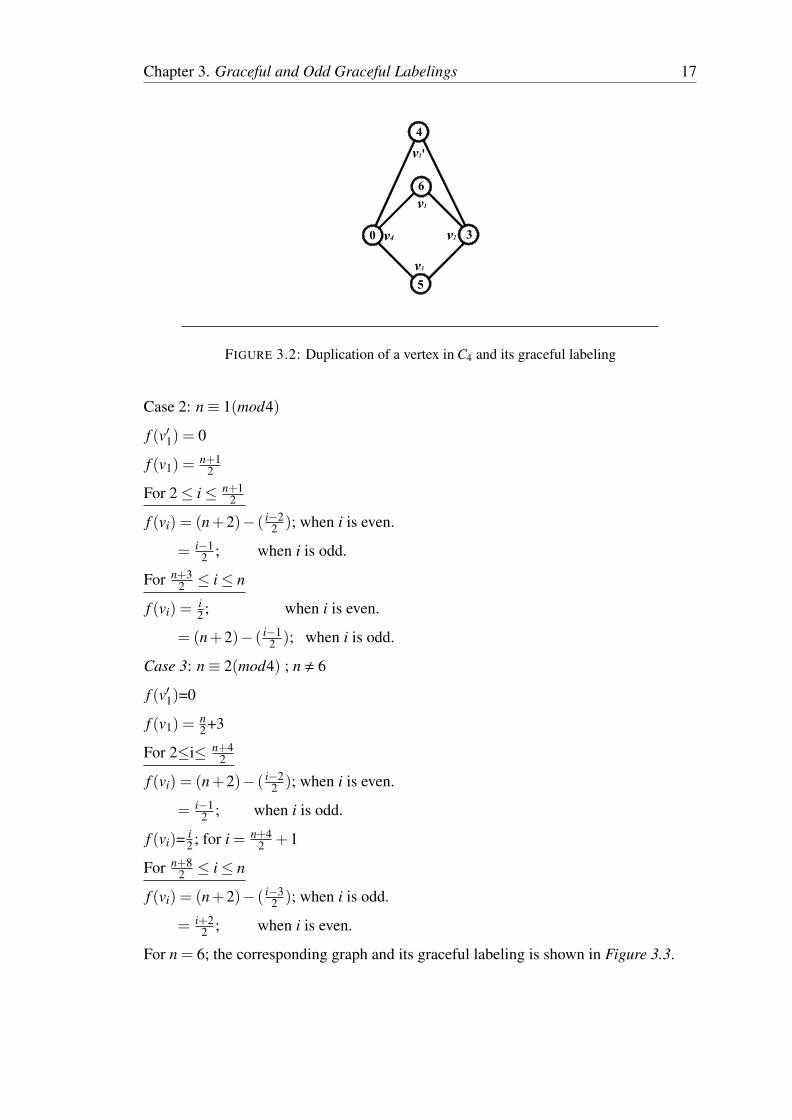
Chapter 3. Graceful and Odd Graceful Labelings 17
v1'
v1
v2
v3
v40
6
3
5
4
FIGURE 3.2: Duplication of a vertex in C4 and its graceful labeling
Case 2: n≡ 1(mod4)
f (v′1) = 0
f (v1) =n+1
2
For 2≤ i≤ n+12
f (vi) = (n+2)− ( i−22 ); when i is even.
= i−12 ; when i is odd.
For n+32 ≤ i≤ n
f (vi) =i2 ; when i is even.
= (n+2)− ( i−12 ); when i is odd.
Case 3: n≡ 2(mod4) ; n , 6
f (v′1)=0
f (v1) =n2+3
For 2≤i≤ n+42
f (vi) = (n+2)− ( i−22 ); when i is even.
= i−12 ; when i is odd.
f (vi)= i2 ; for i = n+4
2 +1
For n+82 ≤ i≤ n
f (vi) = (n+2)− ( i−32 ); when i is odd.
= i+22 ; when i is even.
For n = 6; the corresponding graph and its graceful labeling is shown in Figure 3.3.

Chapter 3. Graceful and Odd Graceful Labelings 18
v1
v2
v3
v4
v5
v6
v1'
1
0
8
4
2
3
6
FIGURE 3.3: Duplication of a vertex in C6 and its graceful labeling
Case 4: n≡ 3(mod4)
f (v′1)=0
f (v1) =n+1
2
For 2≤i≤ n+12
f (vi) = (n+2)− ( i−22 ); when i is even.
= i−12 ; when i is odd.
For n+32 ≤ i≤ n
f (vi) = (n+2)− ( i−12 ); when i is odd.
= i2 ; when i is even.
In view of the above defined labeling pattern f is a graceful labeling for the graph
obtained by the duplication of an arbitrary vertex in cycle Cn. �
Illustration 3.3.2. The graph obtained by duplicating the vertex v1 of cycle C9 is shown
in Figure 3.4.

Chapter 3. Graceful and Odd Graceful Labelings 19
v1
v1'
v2
v3
v4
v5v6
v7
v8
v9
0
11
5
1
10
23
8
4
7
FIGURE 3.4: Duplication of a vertex in C9 and its graceful labeling
Theorem 3.3.3. Duplication of an edge in cycles of even order admits graceful labeling.
Proof. Let v1,v2,. . . , vn be the vertices of the cycle Cn where n is even. Let G be the
graph obtained by duplicating an arbitrary edge of Cn. Without loss of generality assume
that e′ = v′1v′2 be the newly added edge to duplicate the edge e = v1v2 in Cn. To define
f : V →{0,1, . . . ,q} following two cases are to be considered.
Case 1: n≡ 0(mod4); n , 4,n , 8
f (v′1) =n2 +4
f (v′2) =n2
For 1≤ i≤ n2 +2
f (vi) =(n+3)− i−12 ; when i is odd.
= i−22 ; when i is even.
f (vi) = i−12 ; for i = n
2 +3
For n2 +4≤ i≤ n−1
f (vi) =(n+3)− i2 ; when i is even.
= i−12 ; when i is odd.
f (vn) =n2 +2
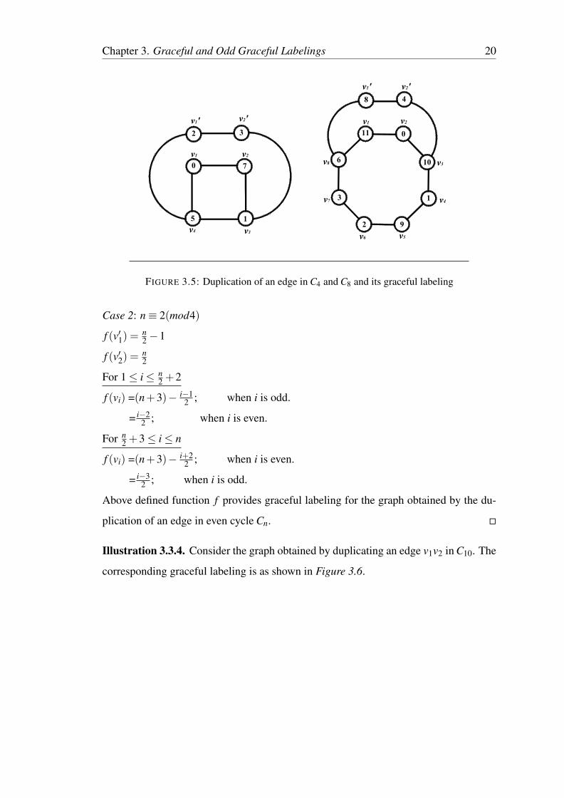
The labeling for the graphs corresponding to C4 and C8 are to be dealt separately. The
graceful labeling is provided in Figure 3.5.
Chapter 3. Graceful and Odd Graceful Labelings 20
v1 v2
v4 v3
v1' v2'
2 3
0 7
5 1
8 4
0
1
92
3
6 10
11
v1 v2
v3
v4
v5v6
v7
v8
v1' v2'
FIGURE 3.5: Duplication of an edge in C4 and C8 and its graceful labeling
Case 2: n≡ 2(mod4)
f (v′1) =n2 −1
f (v′2) =n2
For 1≤ i≤ n2 +2
f (vi) =(n+3)− i−12 ; when i is odd.
= i−22 ; when i is even.
For n2 +3≤ i≤ n
f (vi) =(n+3)− i+22 ; when i is even.
= i−32 ; when i is odd.
Above defined function f provides graceful labeling for the graph obtained by the du-
plication of an edge in even cycle Cn. �
Illustration 3.3.4. Consider the graph obtained by duplicating an edge v1v2 in C10. The
corresponding graceful labeling is as shown in Figure 3.6.
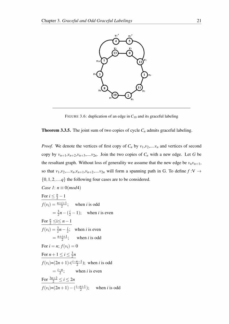
Chapter 3. Graceful and Odd Graceful Labelings 21
v1 v2
v3
v4
v5
v6v7
v8
v9
v10
v1' v2'
13
12
11
10
4 5
0
1
2
8
3
7
FIGURE 3.6: duplication of an edge in C10 and its graceful labeling
Theorem 3.3.5. The joint sum of two copies of cycle Cn admits graceful labeling.
Proof. We denote the vertices of first copy of Cn by v1,v2,....vn and vertices of second
copy by vn+1,vn+2,vn+3,....v2n. Join the two copies of Cn with a new edge. Let G be
the resultant graph. Without loss of generality we assume that the new edge be vnvn+1,
so that v1,v2,....vn,vn+1,vn+2,....v2n will form a spanning path in G. To define f :V →
{0,1,2, ....q} the following four cases are to be considered.
Case 1: n≡ 0(mod4)
For i≤ n2 −1
f (vi) =n+i+1
2 ; when i is odd
= 32n− ( i
2 −1); when i is even
For n2 ≤i≤ n−1
f (vi) =32n− i
2 ; when i is even
= n+i+12 ; when i is odd
For i = n; f (vi) = 0
For n+1≤ i≤ 32n
f (vi)=(2n+1)-( i−n−12 ); when i is odd
= i−n2 ; when i is even
For 3n+22 ≤ i≤ 2n
f (vi)=(2n+1)− ( i−n+12 ); when i is odd
Chapter 3. Graceful and Odd Graceful Labelings 22
= i−n2 ; when i is even
Case 2: n≡ 1(mod4)
f (v1)=0
For 2≤i≤ n−12
f (vi) = n+( i+12 ); when i is odd
= (n+1)− ( i2); when i is even
For n+12 ≤ i ≤ n−1
f (vi) = (n+1)− ( i+12 ); when i is odd
= n+( i+22 ); when i is even
For n≤ i≤ 2n
f (vi) = (2n+1)-( i−n2 ) ; when i is odd
= i+1−n2 ; when i is even
Case 3: n≡ 2(mod4)
For 1≤ i≤ n−2
f (vi)= i2 ; when i is even
= (2n+1)− ( i−12 ); when i is odd
f (vn−1) = f (vn−3)− f (vn−2)−1
f (vn) = 0
For n+1≤ i ≤ 3n2 −1
f (vi)= i−12 ; when i is odd
= (2n+1)-( i−42 ); when i is even
f (vi)= i+12 ; for i=3n
2
For 3n2 +1≤ i≤ 3n
2 +2
f (vi)= i+22 ; when i is even
= (2n+1)-( i−52 ); when i is odd
For 3n2 +3≤ i≤ 2n
f (vi)=(2n+1)-( i−52 ) ; when i is odd
= i+42 ; when i is even
Case 4: n≡ 3(mod4)
1≤ i≤ n−12
f (vi)=3(n+1)
2 − ( i+12 ); when i is odd

Chapter 3. Graceful and Odd Graceful Labelings 23
= n+i+12 ; when i is even
Forn+12 ≤ i≤ n−2
f (vi)=3(n+1)
2 − ( i+22 ); when i is even
= n+i+22 ; when i is odd
f (vn−1) = 0
For n≤ i≤ 2n
f (vi)=(2n+1)-( i−n2 ) ; when i is odd
= i+1−n2 ; when i is even
In the above four cases it is possible to assign labels in such a way that it provides
graceful labeling for joint sum of two copies of cycle Cn. �
Illustration 3.3.6. The graceful labeling of the joint sum of two copies of C13 is as
shown in Figure 3.7.
v1
v2
v3
v4
v5
v6v7
v8
v9
v10
v11
v12v13 v14
v15
v16
v17
v18
v19
v20v21
v22
v23
v24
v25
v26
0
9
8
1
2
3
4
5
6
7
27
13
15
12
16
1110
18
19
20 26
25
24
23
22
21
FIGURE 3.7: Joint sum of two copies of C13 and its graceful labeling
Chapter 3. Graceful and Odd Graceful Labelings 24
3.4 Odd Graceful Graphs
Many illustrious works on graceful labelings provided the reason for different ways
of labeling of graphs. Some variations of graceful labeling are also introduced re-
cently such as edge graceful labeling, Fibonacci graceful labeling, odd graceful label-
ing. Gnanajothi[18] introduced the concept of odd graceful graphs.
3.4.1 Odd Graceful Labeling
A graph G=(V(G),E(G)) with p vertices and q edges is said to admit an odd graceful
labeling if f : V (G)→ {0,1,2, . . . ,2q− 1} is injective and the induced function f* :
E(G)→ {1,3,5, . . . ,2q− 1} defined as f*(e = uv) = | f (u)− f (v)| is bijective. The
graph which admits odd graceful labeling is called an odd graceful graph.
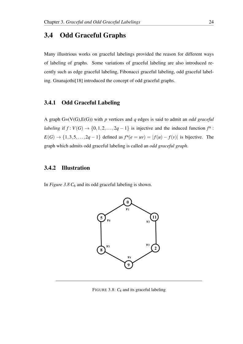
3.4.2 Illustration
In Figure 3.8 C6 and its odd graceful labeling is shown.
0
2
9
8
5 11
v1
v2
v3
v4
v5
v6
FIGURE 3.8: C8 and its graceful labeling

Chapter 3. Graceful and Odd Graceful Labelings 25
3.4.3 Some known results
Gnanajothi[18] has proved that
• Every graph with α-labeling has an odd graceful labeling.
• Every graph with an odd cycle is not odd graceful.
• Pn,Cn are odd graceful if and only if n is even.
• Km,n,combs,books, Pn⊙
K1 are odd graceful graphs.
• Crowns are odd graceful if and only if n is even.
• The disjoint union of copies of C4, one point union of copies of C4 are odd grace-
ful graphs.
• Cn×K2 is odd graceful if and only if n is even.
• Caterpillars, rooted trees of height 2, the graphs obtained from Pn (n ≥ 3) by
adding exactly two leaves at each vertex of degree 2 of Pn admit odd graceful
labeling.
• The graphs obtained from a star by adjoining to each end vertex the path P3 or by
adjoining to each end vertex the path P4 are odd graceful graphs.
• All trees are odd graceful (Conjecture) and it has been proved true for all trees of
order up to 10.
Barrientos[2] has investigated the following results.
• All trees are odd graceful (Conjecture) has been verified for all trees of order up
to 12.
• Disjoint union of caterpillars and all trees of diameter 5 are odd graceful.
• Every bipartite graph is odd graceful (Conjecture).

Chapter 3. Graceful and Odd Graceful Labelings 26
Kathiresan[28] has shown that
• Ladders and graphs obtained from them by subdividing each step exactly once
are odd graceful.
• S(Tn) is odd graceful.
• The planar grids Pm×Pn are odd graceful.
Eldergill[14] has generalized Gnanajothi’s results on stars by showing that the graphs
obtained by joining one end point from each of any odd number of paths of equal length
is odd graceful.
Seoud,Diab,Elsakhawi[38] have shown that a connected complete r-partite graph is odd
graceful if and only if r = 2 and the join of any two connected graph is not odd graceful.
Sekar[37] has investigated that the following graphs are odd graceful.
• Cm⊙
Pn where n≥ 3, m is even.
• All n-polygonal snakes with n is even.
• The split graph of Pn, Cn where n is even.
• Lobsters, banana trees and regular bamboo trees.
• The graph obtained by beginning with C6 and repeatedly forming the one point
union with additional copies of C6 in succession.
• The graph obtained by beginning with C8 and repeatedly forming the one point
union with additional copies of C8 in succession.
• Graphs obtained from even cycles by identifying a vertex of the cycle with the
end point of a star.
Chawathe and Krishna[8] have extended the definition of odd gracefulness to count-
ably infinite graphs and showed that all countably infinite bipartite graphs which are
connected and locally finite have odd graceful labeling.
Chapter 3. Graceful and Odd Graceful Labelings 27
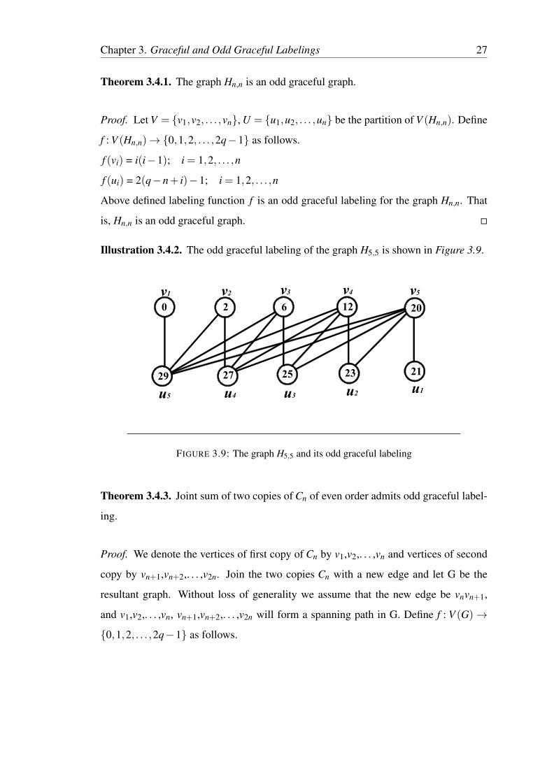
Theorem 3.4.1. The graph Hn,n is an odd graceful graph.
Proof. Let V = {v1,v2, . . . ,vn}, U = {u1,u2, . . . ,un} be the partition of V (Hn,n). Define
f : V (Hn,n)→{0,1,2, . . . ,2q−1} as follows.
f (vi) = i(i−1); i = 1,2, . . . ,n
f (ui) = 2(q−n+ i)−1; i = 1,2, . . . ,n
Above defined labeling function f is an odd graceful labeling for the graph Hn,n. That
is, Hn,n is an odd graceful graph. �
Illustration 3.4.2. The odd graceful labeling of the graph H5,5 is shown in Figure 3.9.
0 2 6 20
2123252729
v1 v2 v3 v4 v5
u5 u4 u3 u2 u1
12
FIGURE 3.9: The graph H5,5 and its odd graceful labeling
Theorem 3.4.3. Joint sum of two copies of Cn of even order admits odd graceful label-
ing.
Proof. We denote the vertices of first copy of Cn by v1,v2,. . . ,vn and vertices of second
copy by vn+1,vn+2,. . . ,v2n. Join the two copies Cn with a new edge and let G be the
resultant graph. Without loss of generality we assume that the new edge be vnvn+1,
and v1,v2,. . . ,vn, vn+1,vn+2,. . . ,v2n will form a spanning path in G. Define f : V (G)→
{0,1,2, . . . ,2q−1} as follows.
Chapter 3. Graceful and Odd Graceful Labelings 28
For 1≤ i≤ n−1
f (vi) = i−1; i is odd.
= 4n− i+3; i is even.
For n≤ i≤ 3n2 +1
f (vi) = i−1; i is even.
= 4n− i+5; i is odd.
For 3n2 +2≤ i≤ 2n
f (vi) = i+1; i is even.
=4n− i+3; i is odd. �
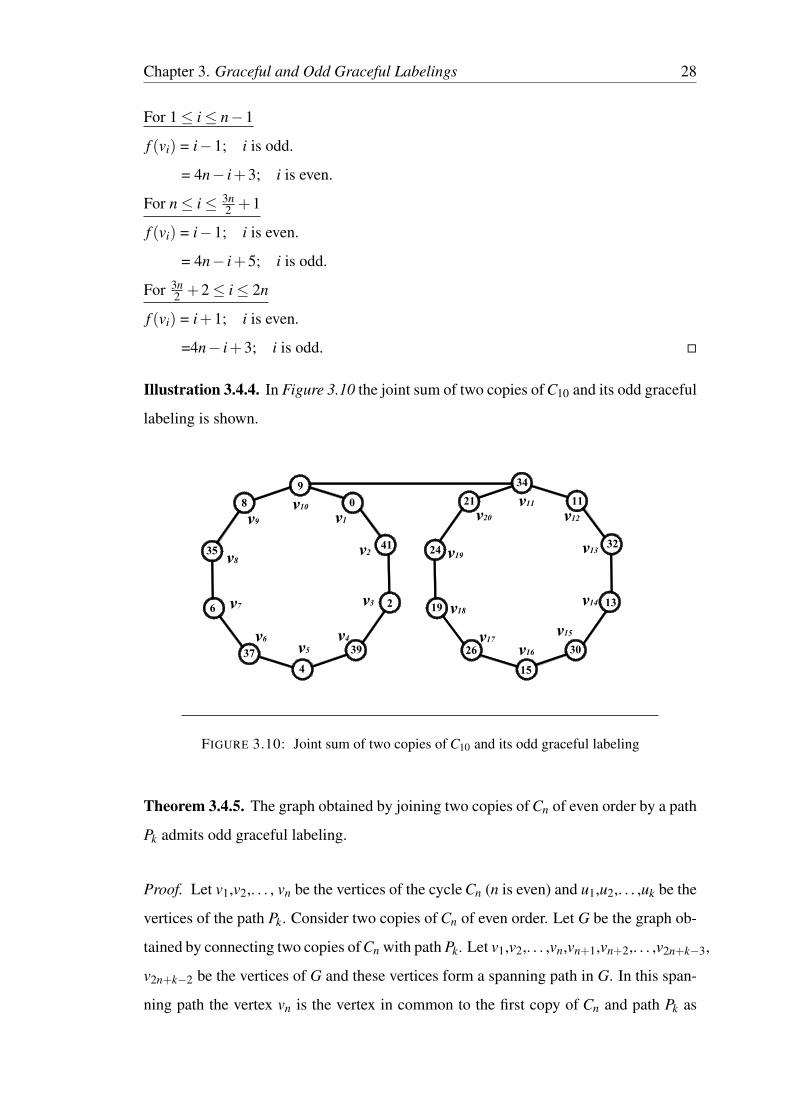
Illustration 3.4.4. In Figure 3.10 the joint sum of two copies of C10 and its odd graceful
labeling is shown.
v3
v1
v2
v4
v5
v6
v7
v8
v9
v11
v12
v13
v14
v15
v16
v17
v18
v19
v20
0
9
41
3937
35
2
4
6
8
34
11
32
13
30
15
26
19
24
21v10
FIGURE 3.10: Joint sum of two copies of C10 and its odd graceful labeling
Theorem 3.4.5. The graph obtained by joining two copies of Cn of even order by a path
Pk admits odd graceful labeling.
Proof. Let v1,v2,. . . , vn be the vertices of the cycle Cn (n is even) and u1,u2,. . . ,uk be the
vertices of the path Pk. Consider two copies of Cn of even order. Let G be the graph ob-
tained by connecting two copies of Cn with path Pk. Let v1,v2,. . . ,vn,vn+1,vn+2,. . . ,v2n+k−3,
v2n+k−2 be the vertices of G and these vertices form a spanning path in G. In this span-
ning path the vertex vn is the vertex in common to the first copy of Cn and path Pk as

Chapter 3. Graceful and Odd Graceful Labelings 29
well as the vertex vn+k−1 is the vertex in common to the second copy of Cn and path Pk.
Define f : V (G)→{0,1,2, . . . ,2q−1} as follows.
For 1≤ i≤ n−1
f (vi) = i−1; i is odd.
=(4n+2k)− (i+1); i is even
For n≤ i≤ 3n2 + k−1
f (vi) = i−1; i is even.
=(4n+2k)− (i−1); i is odd.
For 3n2 + k ≤ i≤ 2n+ k−2
f (vi) = (4n+2k)− (i+1); i is odd.
=i+1; i is even.
In accordance with above labeling pattern the graph under consideration admits odd
graceful labeling. �
Illustration 3.4.6. Consider the graph obtained by attaching two copies of C10 by P5.
The odd graceful labeling is as shown in Figure 3.11.
v1
v2
v3
v4
v5
v6
v7
v8
v9v11 v12 v13 v14
v15
v16
v17
v18v19
v20
v21
v22
v23
v10 0
26
8
9
4
47
4543
41
40 11 38 13
36
15
34
1732
28
23
26
21
FIGURE 3.11: The odd graceful labeling of the graph obtained by attaching two copiesof C10 by P5
Theorem 3.4.7. The graph resulted by identifying an arbitrary vertex of a cycle Cn of
even order with the apex vertex of star K1,m produces an odd graceful graph.

Chapter 3. Graceful and Odd Graceful Labelings 30
Proof. Let v1,v2,. . . , vn be the n vertices of cycle Cn and u,u1,u2,. . . , um be the m+
1 vertices of star K1,m where u is the apex vertex. Let G be the resultant graph by
identifying a vertex of cycle Cn to the apex vertex of star K1,m. Without loss of generality
assume that the vertex v1 in cycle Cn is identified with the apex vertex u in K1,m. To
define f : V (G)→{0,1,2, . . . ,2q−1} the following two cases are to be considered.
Case 1: n≡ 0(mod4)
For 1≤ i≤ n2
f (vi) = i−1; i is odd.
=2(n+m)− (i−1); i is even.
For n2 +1≤ i≤ n
f (vi) = i+1; i is odd.
=2(n+m)− (i−1); i is even.
f (u) = 0
For 2≤ j ≤ m
f (u j) = 2 j−1; ∀ j
Case 2: n≡ 2(mod4)
For 1≤ i≤ n2 +1
f (vi) = i−1; i is odd.
=2(n+m)− (i−1); i is even.
For n2 +2≤ i≤ n
f (vi) = i+1; i is odd.
=2(n+m)− (i+1); i is even.
f (u) = 0
For 2≤ j ≤ m−1
f (u j) = 2 j−1
f (um) = (n+1)−2(3−m)
Above defined function f provides an odd graceful labeling for G. That is, G is an odd
graceful graph. �
Illustration 3.4.8. The graph obtained by identifying a vertex in cycle C14 with the apex
vertex of star K1,5 and its odd graceful labeling is given in Figure 3.12.

Chapter 3. Graceful and Odd Graceful Labelings 31
0
2
4
6
13 5 7
37
35
33
3110
27
12
25
14
23
19
v1 = uv2
v3
v4
v5
v6
v7v8v9
v10
v11
v12
v13
v14
u1
u2 u3 u4
u5
FIGURE 3.12: The odd graceful labeling of the graph obtained by identifying a vertexof cycle C14 with the apex vertex of star K1,5
Theorem 3.4.9. The graph obtained by identifying all the n vertices of cycle Cn of even
order to the apex vertices of n copies of K1,m admits odd graceful labeling.
Proof. Let Cn be a cycle of even order with v1,v2,. . . , vn be its vertices and G be the
graph obtained by identifying all the n vertices vi of Cn with the apex vertices of star
K1,m. Denote the pendant vertices of K1,m by vi j where 1 ≤ i ≤ n and 1 ≤ j ≤ m.
Then G is a graph with |V (G)| = n+ nm and |E(G)| = n+ nm. To define f : V (G)→
{0,1,2, . . . ,2q−1} we consider following two cases.
Case 1: n≡ 0(mod4) .
For 1≤ i≤ n2
f (vi) = (m+1)(2n− i)+1; i is even.
=(m+1)(i−1); i is odd.
For n2 +1≤ i≤ n
f (vi) = (m+1)(2n− i)+1; i is even.
=(m+1)(i−3)+2(m+2); i is odd.
Chapter 3. Graceful and Odd Graceful Labelings 32
For 1≤ i≤ n2 ; 1≤ j ≤ m
f (vi j)=(m+1)(2n− i+1)−2 j+1; if i is odd.
=(m+1)(i−2)+2 j; if i is even.
For n2 +1≤ i≤ n; 1≤ j ≤ m
f (vi j)=(m+1)(2n− i+1)−2 j+1; if i is odd.
=(m+1)(i−4)+2(m+ j+2); if i is even.
Case 2: n≡ 2(mod4)
For 1≤ i≤ n2 +1
f (vi) = (m+1)(2n− i)+1; i is even.
=(m+1)(i−1); i is odd.
For n2 +2≤ i≤ n−1
f (vi) = (m+1)(2n− i)+1; i is even.
=(m+1)(i−3)+2(m+2); i is odd.
f (vn) = (m+1)(2n− i)−1
For 1≤ i≤ n2 ; 1≤ j ≤ m
f (vi j)=(m+1)(2n− i+1)−2 j+1; if i is odd.
=(m+1)(i−2)+2 j; if i is even.
For n2 +1≤ i≤ n−1; 1≤ j ≤ m
f (vi j)=(m+1)(2n− i+1)−2 j+1; if i is odd.
=(m+1)(i−2)+2( j+1); if i is even.
f (vn j)=(m+1)(n−2)+2( j+1); for 1≤ j ≤ m−1
=(m+1)(n−2)+2(2 j+1); for j = m
The above defined function f exhausts all the possibilities and the graph under consid-
eration is an odd graceful graph. �
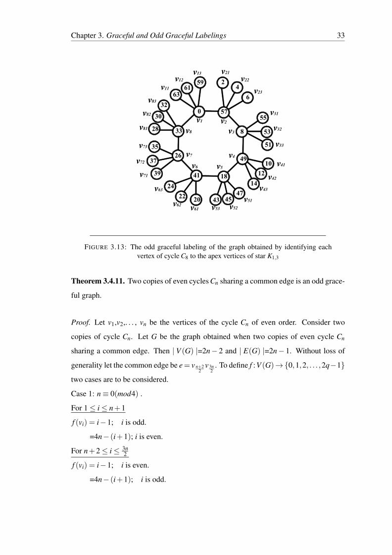
Illustration 3.4.10. Figure 3.13 shows the odd graceful labeling of the graph obtained
by identifying each vertex of C8 to the apex vertices of star K1,3.
Chapter 3. Graceful and Odd Graceful Labelings 33
0
8
24
66361
59
32
30
28
35
37
39
24
2220 43 45
47
14
12
10
51
53
5557
49
1841
26
33
v1 v2
v3
v4
v5v6
v7
v8
v12
v13 v21
v11
v22
v23
v31
v32
v33
v41
v42
v43
v51
v52v53v61v62
v63
v71
v82
v83
v81
v73
v72
FIGURE 3.13: The odd graceful labeling of the graph obtained by identifying eachvertex of cycle C8 to the apex vertices of star K1,3
Theorem 3.4.11. Two copies of even cycles Cn sharing a common edge is an odd grace-
ful graph.
Proof. Let v1,v2,. . . , vn be the vertices of the cycle Cn of even order. Consider two
copies of cycle Cn. Let G be the graph obtained when two copies of even cycle Cn
sharing a common edge. Then | V (G) |=2n− 2 and | E(G) |=2n− 1. Without loss of
generality let the common edge be e= v n+22
v 3n2
. To define f :V (G)→{0,1,2, . . . ,2q−1}
two cases are to be considered.
Case 1: n≡ 0(mod4) .
For 1≤ i≤ n+1
f (vi) = i−1; i is odd.
=4n− (i+1); i is even.
For n+2≤ i≤ 3n2
f (vi) = i−1; i is even.
=4n− (i+1); i is odd.

Chapter 3. Graceful and Odd Graceful Labelings 34
For 3n+22 ≤ i≤ 2n−2
f (vi) = i−1; i is even.
=4n− (i+3); i is odd.
Case 2: n≡ 2(mod4) .
For 1≤ i≤ n
f (vi) = i−1; i is odd.
=4n− (i+1); i is even
For n+1≤ i≤ 3n2
f (vi) = i−1; i is even.
=4n− (i+1); i is odd.
For 3n+22 ≤ i≤ 2n−2
f (vi) = i+1; i is even.
=4n− (i+1); i is odd.
Above defined labeling pattern exhausts all the possibilities and in each case the graph
under consideration admits odd graceful labeling. �
Illustration 3.4.12. In Figure 3.14 the odd graceful labeling of two copies of cycle C8
sharing a common edge is shown.
v1 v2
v3
v4
v5
v14
v13
v6
v7
v8v9
v10
v11
v12
0
2
4
6
29
27
11
16
13
25
23
20
8
9
FIGURE 3.14: The odd graceful labeling of two copies of cycle C8 sharing a commonedge
Chapter 3. Graceful and Odd Graceful Labelings 35
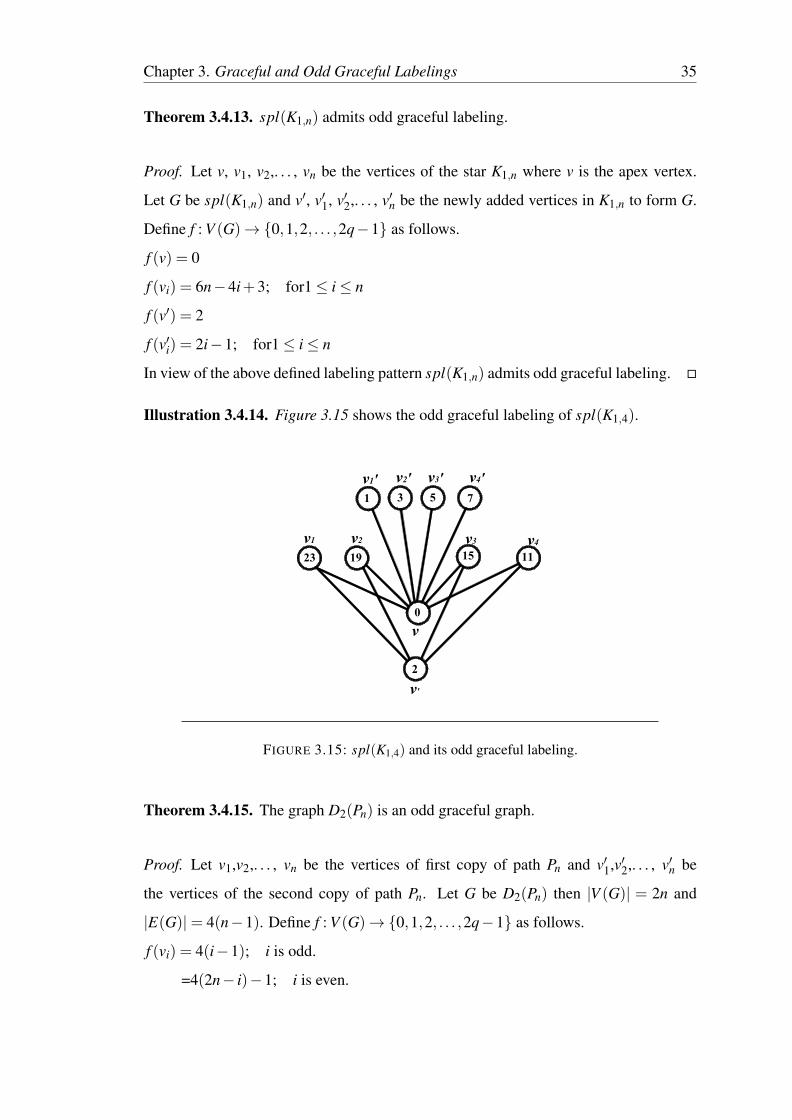
Theorem 3.4.13. spl(K1,n) admits odd graceful labeling.
Proof. Let v, v1, v2,. . . , vn be the vertices of the star K1,n where v is the apex vertex.
Let G be spl(K1,n) and v′, v′1, v′2,. . . , v′n be the newly added vertices in K1,n to form G.
Define f : V (G)→{0,1,2, . . . ,2q−1} as follows.
f (v) = 0
f (vi) = 6n−4i+3; for1≤ i≤ n
f (v′) = 2
f (v′i) = 2i−1; for1≤ i≤ n
In view of the above defined labeling pattern spl(K1,n) admits odd graceful labeling. �
Illustration 3.4.14. Figure 3.15 shows the odd graceful labeling of spl(K1,4).
v'
v
v1 v2 v3 v4
v1' v2' v3' v4'
0
2
1 3 5 7
23 19 15 11
FIGURE 3.15: spl(K1,4) and its odd graceful labeling.
Theorem 3.4.15. The graph D2(Pn) is an odd graceful graph.
Proof. Let v1,v2,. . . , vn be the vertices of first copy of path Pn and v′1,v′2,. . . , v′n be
the vertices of the second copy of path Pn. Let G be D2(Pn) then |V (G)| = 2n and
|E(G)|= 4(n−1). Define f : V (G)→{0,1,2, . . . ,2q−1} as follows.
f (vi) = 4(i−1); i is odd.
=4(2n− i)−1; i is even.

Chapter 3. Graceful and Odd Graceful Labelings 36
f (v′i) = 4(i−1)+2; i is odd.
= 4(2n− i)−5; i is even.
The above defined function f provides graceful labeling for D2(Pn). �
Illustration 3.4.16. The odd graceful labeling of D2(P6) is given in Figure 3.16.
2
0 8
35 10 27 18 19
39 31 16 23
v1' v2' v3' v4' v5' v6'
v1 v2 v3 v4 v5 v6
FIGURE 3.16: D2(P6) and its odd graceful labeling.
Theorem 3.4.17. The graph D2(K1,n) is an odd graceful graph.
Proof. Let v,v1,v2,. . . , vn be the vertices of first copy of star K1,n and v′,v′1,v′2,. . . , v′n
be the vertices of the second copy of star K1,n. Let G be D2(K1,n). Define f : V (G)→
{0,1,2, . . . ,2q−1} as follows.
f (v) = 0
f (vi) = 8n−4i+3; for1≤ i≤ n
f (v′) = 2
f (v′i) = 4i−1; for1≤ i≤ n
In view of above defined labeling pattern G admits odd graceful labeling. �
Illustration 3.4.18. The graph D2(K1,4) and its odd graceful labeling is shown in Figure
3.17.

Chapter 3. Graceful and Odd Graceful Labelings 37
31 27 23 19
151173
0
2
v1 v2 v3 v4
v1' v2' v3' v4'
v
v'
FIGURE 3.17: D2(K1,4) and its odd graceful labeling.
Theorem 3.4.19. K1,n(T p)P2 is an odd graceful graph.
Proof. Let u1, u2,. . . , un,un+1 be the vertices of the star K1,n, where u1 is the apex
vertex. Let v1, v2 be the vertices of P2. Let G be the graph K1,n(T p)K2. We divide the
vertex of G into two disjoint sets T1 = {(ui,v1)/i = 1,2 . . . ,n+1} and T2 = {(ui,v2)/i =
1,2 . . . ,n+1}. Define f : V (G)→{0,1,2, . . . ,2q−1} as follows.
f (ui,v1) = 2(i−1); for 1≤ i≤ n+1
f (u1,v2) = 1
f (ui,v2) = 2(n+ i)−3; for 2≤ i≤ n+1
The above defined function f provides graceful labeling for tensor product of K1,n and
path P2. That is, K1,n(T p)P2 is an odd graceful graph. �
Illustration 3.4.20. In Figure 3.18 the graph K1,4(T p)P2 and its odd graceful labeling
is shown.

Chapter 3. Graceful and Odd Graceful Labelings 38
(u1,v1) (u2,v1) (u3,v1) (u4,v1) (u5,v1)
(u1,v2) (u2,v2) (u3,v2) (u4,v2) (u5,v2)
0 2 4 6 8
1 9 11 13 15
FIGURE 3.18: K1,4(T p)P2 and its odd graceful labeling.
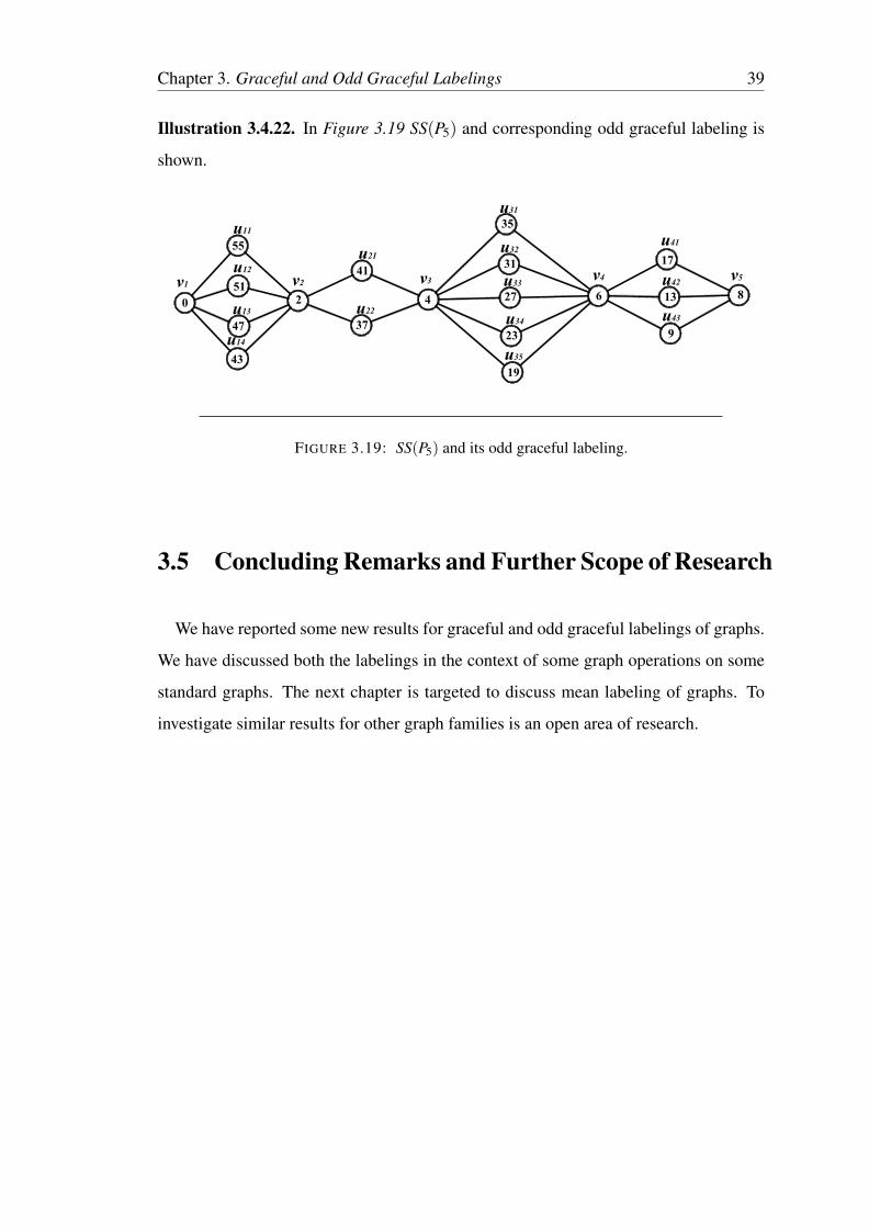
Theorem 3.4.21. SS(Pn) is an odd graceful graph.
Proof. Let Pn be the path containing n vertices v1,v2,. . . ,vn and n−1 edges. Let ei de-
notes the edge vivi+1 in Pn and G be SS(Pn). For 1≤ i≤ n−1 each edge ei of path Pn is
replaced by a complete bipartite graph K2,mi where mi is any positive integer. Let ui j be
the vertices of the mi vertices part of the K2,mi where 1≤ i≤ n−1 and 1≤ j≤max{mi}.
Define f : V (G)→{0,1,2, . . . ,2q−1} as follows.
f (vr) = 2(r−1); For 1≤ r ≤ n
For i = 1
f (ui j)=4n−1
∑k=1
mk−4 j+3; 1≤ j ≤ m1
For i≥ 2 and j = 1
f (ui j)=4n−1
∑k=i
mk +2i−3
For i≥ 2 and j ≥ 2
f (ui j)=4n−1
∑k=i
mk−2(2 j− i)+1
Above defined function f provides an odd graceful labeling for arbitrary supersubdivi-
sion of path Pn. That is, SS(Pn) is an odd graceful graph. �
Chapter 3. Graceful and Odd Graceful Labelings 39
Illustration 3.4.22. In Figure 3.19 SS(P5) and corresponding odd graceful labeling is
shown.
0
55
51
47
43
2
41
37
4
35
31
27
23
19
6
17
13
9
8v1 v2 v3 v4 v5
u11
u12
u13
u14
u21
u22
u31
u32
u33
u34
u35
u41
u42
u43
FIGURE 3.19: SS(P5) and its odd graceful labeling.
3.5 Concluding Remarks and Further Scope of Research
We have reported some new results for graceful and odd graceful labelings of graphs.
We have discussed both the labelings in the context of some graph operations on some
standard graphs. The next chapter is targeted to discuss mean labeling of graphs. To
investigate similar results for other graph families is an open area of research.

Chapter 4
Some New Families of Mean Graphs
40

Chapter 4. Some New Families of Mean Graphs 41
4.1 Introduction
A detailed discussion on graceful and odd graceful labelings is held in the previous
chapter while the present chapter is focused on mean labeling of some graphs. We
investigate some new families of mean graphs and mean labeling in the context of some
graph operations on some standard graphs.
4.2 Mean Labeling
4.2.1 Mean Graph
A function f is called a mean labeling of graph G if f :V (G)→{0,1,2, . . . ,q} is injective
and the induced function f* : E(G)→{1,2, . . . ,q} defined as
f*(e = uv) = f (u)+ f (v)2 ; if f (u)+ f (v) is even
= f (u)+ f (v)+12 ;if f (u)+ f (v) is odd
is bijective.
The graph which admits mean labeling is called a mean graph..
4.2.2 Illustration
In Figure 4.1 K2,3 and its mean labeling is shown.
0 5
642
v1 v2
u1 u2 u3
FIGURE 4.1: K2,3 and its mean labeling

Chapter 4. Some New Families of Mean Graphs 42
4.2.3 Some existing results
The concept of mean labeling was introduced by Somasundaram and Ponraj [41, 42, 43]
and they have proved that
• Pn is mean graph for any n ∈ N.
• Cn is mean graph for any n ∈ N.
• Cm⋃
Pn is mean graph for any m,n ∈ N.
• Pm×Pn is mean graph for any m,n ∈ N.
• Pm×Cn is mean graph for any m,n ∈ N.
• Kn is mean graph if and only if n < 3.
• K1,n is mean graph if and only if n < 3.
• Bm,n is mean graph if and only if m < n+2.
• Subdivision graph of K1,n admits mean labeling if and only if n < 4.
• Wn is not a mean graph for n > 3.
Vaidya and Kanani [45] have proved that
• The graph obtained by the path union of k copies of cycle Cn is a mean graph.
• The graph obtained by joining two copies of cycle Cn by a path Pk is a mean
graph.
• The graph obtained by arbitrary supersubdivion of any path Pn is a mean graph.

Chapter 4. Some New Families of Mean Graphs 43
4.3 Some New Families of Mean Graphs
Observations 4.3.1. We find the following observations.
• v ∈ V (G) and d(v) ≥ 2, having label 0, then edge label 1 can be produced only
if v is adjacent to the vertex having label either 1 or 2 and edge label 2 can be
produced only if v is adjacent to the vertex with label either 3 or 4.
• The edge label q can be produced only when the vertices with labels q and q−1
are adjacent in G.
Theorem 4.3.2. P2n is a mean graph.
Proof. Let v1,v2,....vn be the vertices of path Pn. Define f : V (G)→ {0,1,2, . . . ,q} as
follows.
f (vi) = 2(i−1); for i≤ (n−1)
f (vi) = 2i−3; for i = n
Above defined labeling pattern provides mean labeling for P2n .
That is, P2n is a mean graph. �
Illustration 4.3.3. The graph P29 and the corresponding mean labeling is shown in Fig-
ure 4.2.
0 2 6 8 10 12 14 15
v1 v2 v3 v4 v5 v6 v7 v8 v9
4
FIGURE 4.2: P29 and the its mean labeling

Chapter 4. Some New Families of Mean Graphs 44
Theorem 4.3.4. M(Pn) admits mean labeling.
Proof. Let v1,v2,. . . vn be the vertices and e1,e2,. . . , en−1 be the edges of path Pn. M(Pn)
consists of two types of vertices {v1,v2,. . . , vn} and {e1,e2,. . . , en−1}. Define f :V (M(Pn))→
{0,1,2, . . . ,q} as follows.
f (e1) = 1
f (e2) = 4
f (e3) = 8
f (ei) = 3i−1; 4≤ i≤ (n−1)
f (v1) = 0
f (vi) = 2i−1; for 2≤ i≤ 4
f (vi) = 3i−5; for 5≤ i≤ n
The above defined function f provides mean labeling for M(Pn).
That is, M(Pn) is a mean graph. �
Illustration 4.3.5. The mean labeling for M(P6) is as shown in Figure 4.3
1 4 8 11 14
0 3 5 7 10 13
e1 e2 e3 e4 e5
v1 v2 v3 v4 v6v5
FIGURE 4.3: M(P6) and its mean labeling
Theorem 4.3.6. Crowns are mean graphs.
Proof. Let v1,v2,. . . , vn be the vertices of cycle Cn. Let G1 be the new graph contains
2n vertices v1,v2,. . . , vn,u1,u2,. . . , un and 2n edges ( n edges of cycle Cn together with n
pendant edges. To define f : V (G1)→ {0,1,2, . . . ,q} the following two cases are to be
considered.
Chapter 4. Some New Families of Mean Graphs 45
Case 1: n is odd.
f (v1) = 0
f (u1) = 1
f (vi) = 2i−1; for 2≤ i≤ n+12
f (vi) = 2i; for n+32 ≤ i≤ n
f (ui) = 2i−2; for 2≤ i < n+12
f (ui) = 2i; for i = n+12
f (ui) = 2i−1; for n+32 ≤ i≤ n
Case 2: n is even.
f (v1) = 0
f (u1) = 1
For 2≤ i≤ n2
f (vi) = 2i−1
f (ui) = 2i−2
For n+22 ≤ i≤ n
f (vi) = 2i
f (ui) = 2i−1
The above defined pattern covers all the possibilities and the graph under consideration
admits mean labeling. �
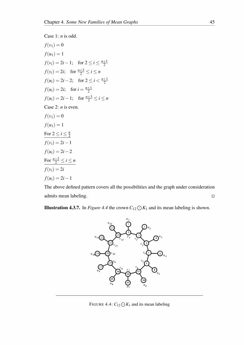
Illustration 4.3.7. In Figure 4.4 the crown C12⊙
K1 and its mean labeling is shown.
16
15
14
13
4
5
7
118
10
0
2
6
9
17
18
19 20
21
22
23
24
u1
3
1
2
u3
u4
u5
u6u7
u8
u9
u10
u11
u12
u1
v 1 v2
v3
v4
v5
v6v7
v8
v9
v 10
v 11
v 12
FIGURE 4.4: C12⊙
K1 and its mean labeling

Chapter 4. Some New Families of Mean Graphs 46
Theorem 4.3.8. Tadpoles T (n,k) admit mean labeling.
Proof. Let v1,v2,. . . , vn be the vertices of cycle Cn and u1,u2,. . . , uk be the vertices of
the path Pk. Let G1 be the resultant graph obtained by identifying a vertex of cycle Cn
to an end vertex of the path Pk. To define f : V (G1)→ {0,1,2, . . . ,q} the following two
cases are to be considered.
Case 1: n is odd.
Identify one of the end vertices of Pk to a vertex of Cn in such a way that v n+32
=u1. We
can label the graph as follows.
f (vi) = 2(i−1); for 1≤ i≤ n+12
f (vi) = 2(n− i)+3; for n+32 ≤ i≤ n
f (u1) = f (v n+32)
f (ui) = n+ i−1, i = 2,3, . . . ,k.
Case 2: n is even.
Identify one of the end vertices of Pk to a vertex of Cn in such a way that v n+22
=u1. We
can label the graph as follows.
f (vi) = 2(i−1); for 1≤ i≤ n+22
f (vi) = 2(n− i)+3; for n+42 ≤ i≤ n
f (u1) = f (v n+22)
f (ui) = n+ i−1, i = 2,3 . . . ,k.
In both the cases the above described function f provides mean labeling for the graph
under consideration. �
Illustration 4.3.9. In Figure 4.5 the tadpole T(9,4) and its mean labeling is shown.
9
8
6
4
20
3
5
7
10 11 12
v1 v2
v3
v4
v5
v6 u1
v7
v8
v9
u2 u3 u4
FIGURE 4.5: T(9,4) and its mean labeling

Chapter 4. Some New Families of Mean Graphs 47
Theorem 4.3.10. T (Pn) is a mean graph.
Proof. Let v1,v2,. . . , vn be the vertices of path Pn with n−1 edges denoted by e1,e2, . . . ,en−1.
Define f : V (T (Pn))→{0,1,2, . . . ,q} as follows.
f (v1) = 0
f (vi) = 4(i−2)+2; for 2≤ i≤ n
f (e j) = 4 j; for 1≤ j ≤ n−2
f (e j) = 4 j−1; for j = n−1
Then f provides mean labeling for T (Pn).
That is, T (Pn) is a mean graph. �
Illustration 4.3.11. The mean labeling of T (P5) is given in Figure 4.6.
0 2 6
4 8
10 14
12 15
v1 v2 v3 v4 v5
e1 e2 e3 e4
FIGURE 4.6: T (P5) and its mean labeling
Theorem 4.3.12. S(Tn) is a mean graph.
Proof. Let Pn be a path on n vertices denoted by (1,1),(1,2), . . . ,(1,n) and has n− 1
edges denoted by e1,e2, . . . ,en−1 where ei is the edge joining the vertices (1, i) and
(1, i+1). The step ladder graph S(Tn) has n2+3n−22 vertices denoted by (1,1),(1,2), . . . ,
(1,n),(2,1),(2,2), . . . ,(2,n),(3,1),(3,2), . . . ,(3,n−1),(4,1),(4,2), . . . ,(4,n−2), . . . ,
(n,1),(n,2). In the ordered pair (i, j), i denotes the row (counted from bottom to top)
and j denotes the column ( from left to right ) in which the vertex occurs. Define
f : V (S(Tn))→{0,1,2, . . . ,q} as follows.

Chapter 4. Some New Families of Mean Graphs 48
f (i,1) = (n2 +n−2)− (i−1); 1≤ i≤ n
f (1, j) = (n2 +n−2)−j−1
∑k=1
(n− k)−j
∑k=2
[(n+ k)− ( j−1)]; 2≤ j ≤ n
f (i, j) = (n2 +n−2)−j−1
∑k=1
(n− k)−j
∑k=2
[(n+ k)− ( j−1)]− (i−1); 2≤ i, j ≤ n;
j , n+2− i
f (i,n+2− i) = i2−2; 2≤ i≤ n
In view of the above defined labeling pattern f is a mean labeling for the step ladder
graph S(Tn). That is, S(Tn) is a mean graph. �
Illustration 4.3.13. Figure 4.7 shows the mean labeling of S(T6).
(1,6)(1,5)(1,4)(1,3)(1,2)
(2,6)(2,5)(2,4)(2,3)(2,2)
(3,5)(3,4)(3,3)(3,2)
(4,4)(4,3)(4,2)
(5,3)(5,2)
0
2
4
3
7
9
8
1018
17
16
15
2324
25
26
27
28
14
(6,2)(6,1)
(5,1)
(4,1)
(3,1)
(2,1)
(1,1)
3435
36
37
38
39
40
FIGURE 4.7: S(T6) and its mean labeling
Theorem 4.3.14. Two copies of cycle Cn sharing a common edge admit mean labeling.
Proof. Let v1,v2,. . . , vn be the vertices of cycle Cn. Consider two copies of Cn. Let G
denote the graph for two copies of cycle Cn sharing a common edge with v1,v2,. . . , v2n−2
is a spanning path. Then | V (G) |=2n− 2 and | E(G) |=2n− 1. To define f : V (G)→
{0,1,2, . . . ,q} the following two cases are to be considered.
Case 1: n is odd.
Without loss of generality assume that e = v n+12
v 3n−12
be the common edge between two
copies of Cn.

Chapter 4. Some New Families of Mean Graphs 49
f (vi) = 2(i−1); for 1≤ i≤ (n+12 )
f (vi) = 2i−1; for n+32 ≤ i≤ n
f (vi) = 2(2n−2− i)+4; for n+1≤ i≤ 3n−32
f (vi) = 2(2n−2− i)+3; for 3n−12 ≤ i≤ 2n−2
Case 2: n is even.
Without loss of generality assume that of edges e = v n+22
v 3n2
be the common edge be-
tween two copies of Cn.
f (vi) = 2(i−1); for 1≤ i≤ (n+22 )
f (vi) = 2i−1; for n+42 ≤ i≤ n
f (vi) = 2(2n−2− i)+4; for n+1≤ i≤ 3n−22
f (vi) = 2(2n−2− i)+3; for 3n2 ≤ i≤ 2n−2
Then above defined function f provides mean labeling for two copies of Cn sharing an
edge. �
Illustration 4.3.15. Figure 4.8 shows mean labeling for two copies of C10 sharing an
edge.
0 2
4
6
8
3
5
7
9 10
13
15
171918
16
14
12
v1 v2
v3
v4
v5
v6
v7
v8
v9
v10v11
v12
v13
v14
v15
v17
v18
v16
FIGURE 4.8: Two copies of C10 sharing an edge and its mean labeling

Chapter 4. Some New Families of Mean Graphs 50
Theorem 4.3.16. D2(K1,n) is a mean graph.
Proof. Consider two copies of K1,n. Let v,v1,v2,. . . , vn be the vertices of the first copy
of K1,n and v′,v′1,v′2,. . . , v′n be the vertices of the second copy of K1,n where v and v′ are
the respective apex vertices. Let G be D2(K1,n). Define f : V (G)→ {0,1,2, . . . ,q} as
follows.
f (v) = 0
f (vi) = 2i; for 1≤ i≤ n
f (v′) = 4n
f (v′1) = 4n−1
f (v′i) = 4n−2i+2; for 2≤ i≤ n
The above defined function provides the mean labeling of the graph D2(K1,n). �
Illustration 4.3.17. The mean labeling of D2(K1,4) is given in Figure 4.9.
0
2 4 6 8
15 14 12 10
16
v1 v2 v3 v4
v1' v2' v3' v4'
v
v'
FIGURE 4.9: D2(K1,4) and its mean labeling
Theorem 4.3.18. D2(Bn,n) is a mean graph.
Proof. Consider two copies of Bn,n. Let {u,v,ui,vi,1≤ i≤ n} and {u′,v′,u′i,v′i,1≤ i≤
n} be the corresponding vertex sets of each copy of Bn,n. Let G be D2(Bn,n). Define
f : V (G)→{0,1,2, . . . ,q} as follows.

Chapter 4. Some New Families of Mean Graphs 51
f (u) = 0
f (ui) = 2i; for 1≤ i≤ n
f (v) = 8n+1
f (vi) = 4i+1; for 1≤ i≤ n−1
f (vn) = 4n+5
f (u′) = 4n
f (u′i) = 2(n+ i); for 1≤ i≤ n−1
f (u′n) = 4n−1
f (v′) = 8n+3
f (v′i) = 8(n+1)−4i; for 1≤ i≤ n
In view of the above defined labeling pattern G admits mean labeling. �
Illustration 4.3.19. The mean labeling of D2(B3,3) is given in Figure 4.10
24
6
0
8
59
1011
12
17
25
27
2824
20
u
u'
u1'u2'
u3'
u1
u2
u3 v1
v2
v3
v1'v2'
v3'
v
v'
FIGURE 4.10: D2(B3,3) and its mean labeling

Chapter 4. Some New Families of Mean Graphs 52
4.4 Mean labeling in the context of some graph opera-
tions
Theorem 4.4.1. The graph obtained by duplicating an arbitrary vertex of Cn admits
mean labeling.
Proof. Let v1,v2,. . . , vn be the vertices of cycle Cn. Let G be the graph obtained by
duplicating an arbitrary vertex of cycle Cn. Without loss generality let this vertex be v1
and the newly added vertex be v′1. To define f : V (G)→ {0,1,2, . . . ,q} the following
two cases are to be considered.
Case 1: n is even.
We define the labeling as follows.
f (v1) = 1
f (v′1) = 4
f (vn) = 0
f (vi) = 2(i+1); For 2≤ i≤ (n2)
f (vi) = 2(n− i)+3; For n2 +1≤ i≤ n−1
Case 2: n is odd.
We define the labeling as follows.
f (v1) = 0
f (v′1) = 5
f (v2) = 4
f (vn) = 1
f (vi) = 2i+1; for 3≤ i≤ (n+12 )
f (vi) = 2(n− i+2); for n+32 ≤ i≤ n−1
Hence f is a mean labeling of the graph G. Thus the graph obtained by duplicating an
arbitrary vertex in cycle Cn is a mean graph. �
Illustration 4.4.2. Consider the graph G obtained by duplicating the vertex v1 of the
cycle C6. It’s mean labeling is given in Figure 4.11

Chapter 4. Some New Families of Mean Graphs 53
v1
v2
v3
v4
v5
v6
v1'
1
4
6
8
7
5
0
FIGURE 4.11: Duplication of a vertex in C6 and its mean labeling
Theorem 4.4.3. The graph obtained by duplicating an arbitrary edge in cycle Cn is a
mean graph.
Proof. Let v1,v2,. . . , vn be the vertices of cycle Cn. Let G be the graph obtained by
duplicating an arbitrary edge in cycle Cn. Without loss of generality let this edge be
e = v1v2 and the newly added edge be e = v′1v′2. To define f : V (G)→{0,1,2, . . . ,q} the
following two cases are to be considered.
Case 1: n is even.
We define the labeling as follows.
f (v1) = 1
f (v2) = 0
f (v′1) = n+3
f (v′2) = n+2
f (vi) = (n+4)− i; if 3≤ i≤ (n2 +1)
f (vi) = n2 +1; if i=n
2 +2
f (vi) = n2 −1; if i=n
2 +3
f (vi) = (n+2)− i; if i≥ n2 +4
Case 2: n is odd.
We define the labeling as follows.

Chapter 4. Some New Families of Mean Graphs 54
f (v1) = 1
f (v2) = 0
f (v′1) = n+3
f (v′2) = n+2
f (vi) = (n+4)− i; if 3≤ i≤ (n+32 )
f (vi) = n+12 ; if i=n+5
2
f (vi) = n−32 ; if i=n+7
2
f (vi) = (n+2)− i; if i≥ n+92
In view of the above defined labeling G admits mean labeling, that is the graph obtained
by duplicating an arbitrary edge in cycle Cn is a mean graph. �
Illustration 4.4.4. Consider the graph G obtained by duplicating the edge e = v1v2 of
the cycle C9. Mean labeling of G is shown in Figure 4.12.
v1 v2
v3
v4
v5v6
v7
v8
v9
v1' v2'1 0
2
3
57
8
9
10
12 11
FIGURE 4.12: Duplication of an edge in C9 and its mean labeling
Theorem 4.4.5. The joint sum of two copies of Cn admits mean labeling.
Proof. We denote the vertices of first copy of Cn by v1,v2,. . . , vn and the vertices of the
second copy of Cn by vn+1,vn+2,. . . , v2n. Let G be the graph obtained by joining an
arbitrary vertex of the first copy of Cn to an arbitrary vertex of second copy of Cn with
a new edge. Let this new edge be vnvn+1 so that v1,v2,. . . , vn,vn+1,vn+2,. . . , v2n forms a
spanning path in G. To define f : V (G)→{0,1,2, . . . ,q} we consider two cases.

Chapter 4. Some New Families of Mean Graphs 55
Case 1: n is even.
f (vi) = 2i; if 1≤ i≤ (n2)
f (vi) = 2(n− i)+1; if n2 +1≤ i≤ n−1
f (vi) = 0; if i = n.
f (vi) = 2n+1; if i = n+1.
f (vi) = 2(2n− i)+4; if n+2≤ i≤ 3n2
f (vi) = 2(i−n)−1; if i≥ 3n2 +1
Case 2: n is odd.
f (vi) = 2i; if 1≤ i≤ (n−12 )
f (vi) = 2(n− i)+1; if n+12 ≤ i≤ n−1
f (vi) = 0; if i = n.
f (vi) = 2n+1; if i = n+1.
f (vi) = 2(2n− i)+4; if n+2≤ i≤ 3n+32
f (vi) = 2(i−n)−1; if i≥ 3n+52
The above defined labeling pattern exhausts both the possibilities for n and in each case
the graph G is a mean graph. �
Illustration 4.4.6. Consider the graph G which is the joint sum of two copies of C10.
The mean labeling is given in the following Figure 4.13.
v1
v2
v3
v4v5
v6
v7
v8
v9v10 v11
v12
v13
v14
v15
v16v17
v18
v19
v20
0
2
4
6
8
5
7
910
2120
18
16
14
1113
15
17
193
FIGURE 4.13: The joint sum of two copies of C10 and its mean labeling
Chapter 4. Some New Families of Mean Graphs 56
Theorem 4.4.7. Fusion of two vertices vi and v j with d(vi,v j)≥ 3 in cycle Cn produces
a mean graph.
Proof. We consider Cn with n vertices v1,v2,. . . , vn. Let the vertex v1 be fused with
vk and the resultant graph be G1 = Cn− vk. To define f : V (G1)→ {0,1,2, . . . ,q} we
consider the following four cases.
Case 1: n≡ 0(mod2) and k ≡ 0(mod2)
We label the graph as follows.
f (v1) = k−1
f (vi) = 2( k2 − i)+2 ; if 2≤ i≤ ( k
2)
f (vi) = 0 ; if i = k2 +1.
f (vi) = 2(i− k2)−1; if k
2 +2≤ i≤ k−1; k , 4, (if k = 4 omit this step and go to the
next step.)
f (vi) = 2i− (k+1); if k+1≤ i≤ n+k2
f (vi) = 2(n− i)+(k+2); if i≥ n+k+22 .
Case 2: n≡ 0(mod2) and k ≡ 1(mod2)
We label the graph as follows.
f (v1) = k−1
f (vi) = 2(k+12 − i)+1 ; if 2≤ i≤ (k−1
2 )
f (vi) = 0 ; if i = k+12 .
f (vi) = 2(i− k+12 ); if k+3
2 ≤ i≤ k−1
f (vi) = 2i− (k+1); if k+1≤ i≤ n+k+12
f (vi) = 2(n− i)+(k+2); if i≥ n+k+32 .
Case 3: n≡ 1(mod2) and k ≡ 0(mod2)
We label the graph as follows.
f (v1) = k−1
f (vi) = 2( k2 − i)+2 ; if 2≤ i≤ ( k
2)
f (vi) = 0 ; if i = k2 +1.
f (vi) = 2(i− k2)−1; if k
2 +2≤ i≤ k−1; k , 4, (if k = 4 omit this step and go to the
next step.)
f (vi) = 2i− (k+1); if k+1≤ i≤ n+k+12
f (vi) = 2(n− i)+(k+2); if i≥ n+k+32 .
Chapter 4. Some New Families of Mean Graphs 57
Case 4: n≡ 1(mod2) and k ≡ 1(mod2)
We label the graph as follows.
f (v1) = k−1 f (vi) = 2(k+12 − i)+1; if 2≤ i≤ (k−1
2 )
f (vi) = 0; if i = k+12 .
f (vi) = 2(i− k+12 ); if k+3
2 ≤ i≤ k−1
f (vi) = 2i− (k+1); if k+1≤ i≤ n+k+22
f (vi) = 2(n− i)+(k+2); if i≥ n+k+42 .
In all the four cases it is possible to assign labels in such a way that the graph G1 under
consideration admits mean labeling. �
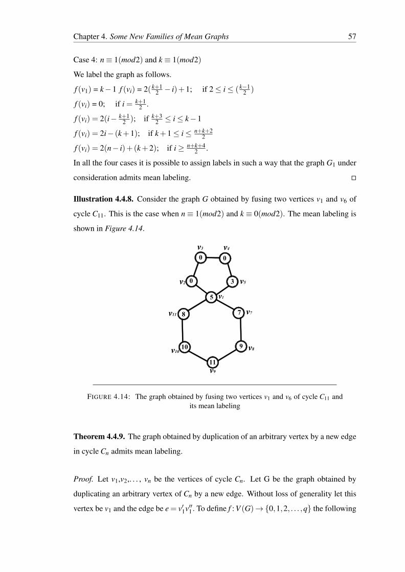
Illustration 4.4.8. Consider the graph G obtained by fusing two vertices v1 and v6 of
cycle C11. This is the case when n≡ 1(mod2) and k ≡ 0(mod2). The mean labeling is
shown in Figure 4.14.
v1
v2
v3 v4
v5
v7
v8
v9
v10
v11
0
3
5
0
0
7
9
8
11
10
FIGURE 4.14: The graph obtained by fusing two vertices v1 and v6 of cycle C11 andits mean labeling
Theorem 4.4.9. The graph obtained by duplication of an arbitrary vertex by a new edge
in cycle Cn admits mean labeling.
Proof. Let v1,v2,. . . , vn be the vertices of cycle Cn. Let G be the graph obtained by
duplicating an arbitrary vertex of Cn by a new edge. Without loss of generality let this
vertex be v1 and the edge be e = v′1v′′1. To define f : V (G)→{0,1,2, . . . ,q} the following

Chapter 4. Some New Families of Mean Graphs 58
two cases are to be considered.
Case 1: n is odd.
We define the labeling as follows.
f (v1) = 3
f (v1′) = 0
f (v1′′) =2
f (vi) = 2(i+1); for 2≤ i≤ (n+12 )
f (vi) = 2(n+3− i)−1; for n+32 ≤ i≤ n
Case 2: n is even.
We define the labeling as follows.
f (v1) = 3
f (v1′) = 0
f (v1′′) =2
f (vi) = 2(i+1); for 2≤ i≤ (n2)
f (vi) = 2(n+3− i)−1; for n+22 ≤ i≤ n
Above defined labeling pattern exhausts all the possibilities and in each case the graph
under consideration admits mean labeling. �
Illustration 4.4.10. Consider the graph obtained by duplicating the vertex v1 by an edge
v′1v′′1 in C8. This is the case when n is even. Corresponding mean labeling is as shown
in Figure 4.15.
0 2
3
6
8
10
11
9
7
5
v1' v1''
v1
v2
v3
v4
v5
v6
v7
v8
FIGURE 4.15: Duplication of the vertex v1 by an edge v′1v′′1 in C8 and its mean labeling

Chapter 4. Some New Families of Mean Graphs 59
Theorem 4.4.11. Duplication of an arbitrary edge by a new vertex in cycle Cn produces
a mean graph.
Proof. Let v1,v2,. . . , vn be the vertices of cycle Cn. Let G be the resultant graph obtained
by duplicating an arbitrary edge in Cn by a new vertex. Without loss of generality let
this edge be e = v1v2 and the vertex be v′. To define f : V (G)→ {0,1,2, . . . ,q} the
following two cases are to be considered.
Case 1: n is odd.
We define the labeling as follows.
f (v′) = 0
f (v1) = 4
f (v2) = 2
f (vi) = 2i; for 3≤ i≤ (n+12 )
f (vi) = 2(n+2− i)+1; for n+32 ≤ i≤ n
Case 2: n is even.
We define the labeling as follows.
f (v′) = 0
f (v1) = 4
f (v2) = 2
f (vi) = 2i; for 3≤ i≤ (n+22 )
f (vi) = 2(n+2− i)+1; for n+42 ≤ i≤ n
In view of the above defined labeling pattern the graph under consideration admits mean
labeling. �
Illustration 4.4.12. Consider the graph obtained by duplicating an arbitrary edge v1v2
by a vertex v′ in cycle C9. It’s mean labeling is as shown in Figure 4.16.

Chapter 4. Some New Families of Mean Graphs 60
0
6
1011
9
7
5
4
v'
v1 v2
v3
v4
v5
v6
v7
v8
v9
8
2
FIGURE 4.16: The graph obtained by duplicating an arbitrary edge v1v2 by a vertex v′
in C9 and its mean labeling
Theorem 4.4.13. The graph obtained by the mutual duplication of a pair of vertices in
two copies of cycle Cn admits mean labeling.
Proof. Let v1,v2,. . . , vn be the vertices of the first copy of cycle Cn and let u1,u2,. . . ,
un be the vertices of the second copy of cycle Cn. Let G be the graph obtained by the
mutual duplication of a pair of vertices each respectively from each copy of cycle Cn.
To define f : V (G)→{0,1,2, . . . ,q} the following two cases are to be considered.
Case 1: n is odd.
Without loss of generality assume that the vertex v n+32
from the first copy of cycle Cn
and the vertex u1 from the second copy of cycle Cn are mutually duplicated.
f (vi) = 2i−2; for 1≤ i≤ n+12
f (vi) = 2(n− i)+3; for n+32 ≤ i≤ n
f (u1) = n+4
f (ui) = n+2i+3; for 2≤ i≤ n+12
f (ui) = 3n−2i+6; for n+32 ≤ i≤ n
Case 2: n is even.
Without loss of generality assume that the vertex v n+22
from the first copy of cycle Cn
and the vertex u1 from the second copy of cycle Cn are mutually duplicated.

Chapter 4. Some New Families of Mean Graphs 61
f (vi) = 2i−2; for 1≤ i≤ n+22
f (vi) = 2(n− i)+3; for n+42 ≤ i≤ n
f (u1) = n+4
f (ui) = n+2i+3; for 2≤ i≤ n2
f (ui) = 3n−2i+6; for n+22 ≤ i≤ n
In view of the above defined labeling pattern f is a mean labeling for the graph obtained
by the mutual duplication of a pair of vertices in cycle Cn. �
Illustration 4.4.14. Figure 4.17 shows mean labeling of the graph obtained by the mu-
tual duplication of a pair of vertices in two copies of cycle C10.
02
4
6
8
3
5
7
9
1417
19
21
2324
22
20
18
16
10
v1v2
v3
v4
v5v6v7
v8
v9
v10
u1 u2
u3
u4
u5u6
u7
u8
u9
u10
FIGURE 4.17: The graph obtained by the mutual duplication of a pair of vertices intwo copies of cycle C10 and its mean labeling
Theorem 4.4.15. The graph obtained by the mutual duplication of a pair of edges in
two copies of cycle Cn admits mean labeling.
Proof. Let v1,v2,. . . , vn be the vertices of the first copy of cycle Cn and let u1,u2,. . . ,
un be the vertices of the second copy of cycle Cn. Let G be the graph obtained by the
mutual duplication of a pair of edges each respectively from each copy of cycle Cn. To
define f : V (G)→{0,1,2, . . . ,q} two cases are to be considered.
Case 1: n is odd.
Without loss of generality assume that the edge e= v n+12
v n+32
from the first copy of cycle

Chapter 4. Some New Families of Mean Graphs 62
Cn and the edge e′= u1u2 from the second copy of cycle Cn are mutually duplicated.
f (v1) = 0 f (vi) = 2i−1; for 2≤ i≤ n+12
f (vi) = 2(n− i)+2; for n+32 ≤ i≤ n
f (ui) = n+2i+2; for 1≤ i≤ n+12
f (ui) = 3n−2i+7; for n+32 ≤ i≤ n
Case 2: n is even.
Without loss of generality assume that the edge e= v n2+1v n
2+2 from the first copy of cycle
Cn and the edge e′= u1u2 from the second copy of cycle Cn are mutually duplicated.
f (vi) = 2i−2; for 1≤ i≤ n2 +1
f (vi) = 2(n− i)+3; for n2 +2≤ i≤ n
f (ui) = n+2i+2; for 1≤ i≤ n2 +1
f (ui) = 3n−2i+7; for n2 +2≤ i≤ n
Then above defined function f provides mean labeling for the graph obtained by the
mutual duplication of a pair of edges in Cn. �
Illustration 4.4.16. Figure 4.18 shows mean labeling of the graph obtained by the mu-
tual duplication of a pair of edges in two copies of cycle C9.
03
5
2
4
6
8 9
7
13 15
17
19
2122
20
18
16
v2v1
v3
v4
v5v6v7
v8
v9
u1 u2
u3
u4
u5u6u7
u8
u9
FIGURE 4.18: The graph obtained by the mutual duplication of a pair of edges in twocopies of cycle C9 and its mean labeling
Theorem 4.4.17. The composition of paths Pm and P2 denoted as Pm[P2] admits mean
labeling except for m = 2.

Chapter 4. Some New Families of Mean Graphs 63
Proof. Let u1,u2,. . . , um be the vertices of the path Pm and v1,v2 be the vertices on the
path P2. The composition Pm[P2] consists of 2m vertices, can be partitioned into two sets
T1={(ui,v1), i = 1,2, . . . ,m} and T2={(ui,v2), i = 1,2, . . . ,m}. To define f : V (Pm[P2])→
{0,1,2, . . . ,q} following three cases are to be considered.
Case 1: m is even, m , 2
We define the labeling as follows.
f (u1,v1) = 0
f (u1,v2) = 2
f (u2,v1) = 4
f (u2,v2) = 7
For 3≤ i≤ (m−1)
f (ui,v1) = f (ui−1,v1)+5; ∀i.
f (ui,v2) = f (ui−1,v2)+6; when i is odd.
= f (ui−1,v2)+4; when i is even
For i = m;
f (ui,v1) = f (ui−1,v1)+6
f (ui,v2) = f (ui−1,v2)+3
Case 2: m is odd.
We define the labeling as follows.
f (u1,v1) = 0
f (u1,v2) = 2
For 2≤ i≤ m
f (ui,v1) = f (ui−1,v1)+6; when i is odd.
= f (ui−1,v1)+4; when i is even.
For 3≤ i≤ (m−1)
f (ui,v2) = f (ui−1,v2)+6; when i is even.
= f (ui−1,v2)+4; when i is odd.
For i = m;
f (ui,v1) = f (ui−1,v1)+6
f (ui,v2) = f (ui−1,v2)+3
In accordance with above labeling pattern the graph under consideration admits mean
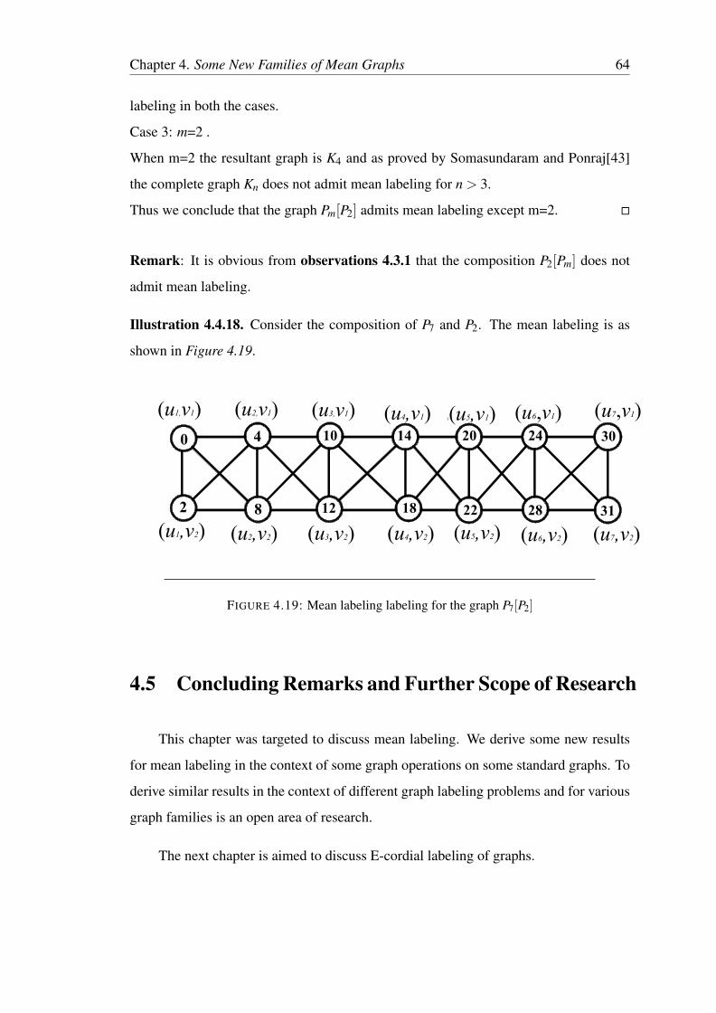
Chapter 4. Some New Families of Mean Graphs 64
labeling in both the cases.
Case 3: m=2 .
When m=2 the resultant graph is K4 and as proved by Somasundaram and Ponraj[43]
the complete graph Kn does not admit mean labeling for n > 3.
Thus we conclude that the graph Pm[P2] admits mean labeling except m=2. �
Remark: It is obvious from observations 4.3.1 that the composition P2[Pm] does not
admit mean labeling.
Illustration 4.4.18. Consider the composition of P7 and P2. The mean labeling is as
shown in Figure 4.19.
0 4 10 14 20 24 30
2 8 12 18 22 28 31
(u1,v1) (u2,v1) (u3,v1) (u4,v1) 1(u5,v1) (u6,v1) (u7,v1)
(u1,v2) (u2,v2) (u3,v2) (u4,v2) (u5,v2) (u6,v2) (u7,v2)
FIGURE 4.19: Mean labeling labeling for the graph P7[P2]
4.5 Concluding Remarks and Further Scope of Research
This chapter was targeted to discuss mean labeling. We derive some new results
for mean labeling in the context of some graph operations on some standard graphs. To
derive similar results in the context of different graph labeling problems and for various
graph families is an open area of research.
The next chapter is aimed to discuss E-cordial labeling of graphs.
Chapter 5
E-cordial Labeling of Graphs
65

Chapter 5. E-cordial Labeling of Graphs 66
5.1 Introduction
In 1987 the concept of cordial labeling was introduced by Cahit [6] as a weaker
version of graceful and harmonious labeling. After that some more labelings are also
introduced having cordial theme. Some of them are A-cordial labeling, product cordial
labeling, total product cordial labeling and E-cordial labeling. This chapter is focused
on E-cordial labeling.
5.2 E-cordial labeling
5.2.1 Binary vertex labeling
Let G be a graph. A mapping f : V (G)→ {0,1} is called a binary vertex labeling of
G and f (v) is called the label of the vertex v of G under f . For an edge e = uv, the
induced edge labeling f ∗ : E(G)→ {0,1} is given by f ∗(e = uv) = | f (u)− f (v)|. Let
v f (0), v f (1) be the number of vertices of G having labels 0 and 1 respectively under
f and let e f (0), e f (1) be the number of edges of G having labels 0 and 1 respectively
under f ∗.
5.2.2 Cordial labeling
A binary vertex labeling of a graph G is cordial labeling if |v f (0)− v f (1)| ≤ 1 and
|e f (0)− e f (1)| ≤ 1.
A graph is cordial if it admits cordial labeling.
5.2.3 Edge graceful labeling
A graph G = (V (G),E(G)) with p vertices and q edges is said to be edge graceful if
there exists a bijection f : E(G) −→ {1,2, . . . ,q} such that the induced mapping f ∗:

Chapter 5. E-cordial Labeling of Graphs 67
V (G)−→{0,1,2, . . . , p−1} given by f ∗(x) = (∑ f (xy))(mod p) taken over all edges xy
is a bijection.
In 1985 Lo[32] has introduced the notion of edge-graceful graphs.
5.2.4 E-cordial labeling-A weaker version of edge graceful labeling
In 1997 Yilmaz and Cahit [49] introduced E-cordial labeling as a weaker version of
edge graceful labeling having blend of cordial labeling and harmonious labeling.
A function f : E(G)→ {0,1} is called an E-cordial labeling of a graph G if the in-
duced function f ∗ : V (G)→ {0,1} defined by f ∗ = ∑{ f (uv)/uv ∈ E(G)}(mod2) and
the number of vertices labeled 0 and the number of vertices labeled 1 differ by at most 1
and the number of edges labeled 0 and the number of edges labeled 1 differ by at most
1.
A graph that admits E-cordial labeling is called E-cordial.
5.2.5 Illustration
In Figure 5.1 K4 and its E-cordial labeling is shown.
0
0
0
0
0
1
1
11
1
v1 v2
v4 v3
FIGURE 5.1: K4 and its E-cordial labeling

Chapter 5. E-cordial Labeling of Graphs 68
5.2.6 Some existing results
Yilmaz and Cahit [49] have proved that
• The trees with n vertices is E-cordial if and only if n . 2(mod4).
• Cn is E-cordial if and only if n . 2(mod4).
• Kn is E-cordial if and only if n . 2(mod4).
• Regular graphs of degree 1 on 2n vertices is E-cordial if and only if n is even.
• Friendship graph C(n)3 is E-cordial ∀n.
• Fan Fn is E-cordial if and only if n . 1(mod4).
• Wheel Wn is E-cordial if and only if n . 1(mod4).
• Km,n admits E-cordial labeling if and only if m+n . 2(mod4).
• The graphs with p≡ 2(mod4) can not be E-cordial.
Devaraj [12] has proved that
• Mm,n which is the the mirror graph of Km,n is E-cordial when m+n is even.
• The general Petersen graph Pn,k is E-cordial when n is even.
Vyas [47] has discussed the E-cordial labeling of some mirror graphs.

Chapter 5. E-cordial Labeling of Graphs 69
5.3 E-cordial labeling of some graphs
Theorem 5.3.1. M(Pn) admits E-cordial labeling.
Proof. Let v1,v2,. . . , vn be the vertices and let e1,e2,. . . , en−1 be the edges of path Pn.
Let M(Pn) be the middle graph of path Pn. According to the definition of the middle
graph V (M(Pn)) = V (Pn)⋃
E(Pn) and E(M(Pn)) = {viei;1 ≤ i ≤ n− 1,viei−1;2 ≤ i ≤
n,eiei+1;1≤ i≤ n−2}. To define f : E(M(Pn))→{0,1} two cases are to be considered.
Case 1: n is even.
f (v1e1) = 0
f (viei) = 1 ; for 2≤ i≤ n−1
f (viei−1) = 0; for 2≤ i≤ n−1
f (vnen−1) = 1.
For 1≤ i≤ n−2
f (eiei+1) = 1; if i is odd.
=0 ; if i is even.
Case 2: n is odd.
f (v1e1) = 0
f (viei) = 1; for 2≤ i≤ n−1
f (viei−1) = 0; for 2≤ i≤ n
For 1≤ i≤ n−2
f (eiei+1) = 1; if i is odd.
=0; if i is even.
In view of the above defined labeling pattern f satisfies the conditions for E-cordial
labeling as shown in Table 5.1. That is, M(Pn) admits E-cordial labeling. �
n Vertex Condition Edge Condition
Even v f (1) = v f (0)+1 = n e f (0) = e f (1) = 3n−42
Odd v f (0) = v f (1)+1 = n e f (0) = v f (1)+1 = 3n−32
Table 5.1
Illustration 5.3.2. In Figure 5.2 M(P6) and its E-cordial labeling is shown.

Chapter 5. E-cordial Labeling of Graphs 70
0 0 0 0 0
0 0
1 1 1 1 1
1 1
1 1 1 1 10
0 0 0 01
e1 e2 e3 e4 e5
v1 v2 v3 v4 v5 v6
FIGURE 5.2: M(P6) and its E-cordial labeling
Theorem 5.3.3. T (Pn) is E- cordial.
Proof. Let v1,v2,. . . , vn be the vertices and e1,e2,. . . , en−1 be the edges of path Pn. Let
T (Pn) be the total graph of path Pn with V (T (Pn)) = V (G)∪ E(G) and E(T (Pn)) =
{vivi+1;1≤ i≤ n−1,viei;1≤ i≤ n−1,eiei+1;1≤ i≤ n−2,viei−1;2≤ i≤ n}. Define
f : E(T (Pn))→{0,1} as follows.
For 1≤ i≤ n−1
f (vivi+1) = 1; if i is odd.
=0; if i is even.
For 1≤ i≤ n−1
f (viei) = 0 ; if i is odd.
=1; if i is even.
For 1≤ i≤ n−2
f (eiei+1) = 0 ; if i is odd.
=1; if i is even.
For 2≤ i≤ n
f (viei−1) = 1 ; if i is odd.
=0; if i is even.
Thus above defined function f satisfies the conditions of E-cordial labeling as shown in
Table 5.2. That is, f provides E-cordial labeling for the graph T (Pn). �

Chapter 5. E-cordial Labeling of Graphs 71
n Vertex Condition Edge Condition
Even v f (1) = v f (0)+1 = n e f (0) = e f (1)+1 = 2n−2
Odd v f (0) = v f (1)+1 = n e f (0) = e f (1)+1 = 2n−2
Table 5.2
Illustration 5.3.4. In Figure 5.3 T (P7) and its E-cordial labeling is shown.
0 0 0 0 0 0
0 0 0
0 0 0
1 1 1 1 1 1
1 1 1
1 1e1 e2 e3 e4 e5 e6
v1 v2 v3 v4 v5 v6 v7
1 1
1 1 1 1
0
0
0 0 0 0
0
FIGURE 5.3: T (P7) and its E-cordial labeling
Theorem 5.3.5. spl(Pn) is E-cordial for even n.
Proof. Let v1,v2,. . . , vn be the vertices and e1,e2,. . . , en−1 be the edges of path Pn. Let
v′1,v′2,. . . , v′n be the newly added vertices to form the split graph of path Pn. Let spl(Pn)
be the split graph of path Pn. V (spl(Pn)) = {vi}⋃{v′i}, 1 ≤ i ≤ n and E(spl(Pn)) =
{v′ivi+1;1 ≤ i ≤ n−1,v′ivi−1;2 ≤ i ≤ n,vivi+1;1 ≤ i ≤ n−1}. Define f : E(spl(Pn))→
{0,1} as follows.
For 1≤ i≤ n−1
f (v′ivi+1) = 0; if i is odd.
=1; if i is even.
For 2≤ i≤ n
f (v′ivi−1) = 0 ; if i is odd.
=1; if i is even.
For 1≤ i≤ n−1
f (vivi+1) = 1 ; if i is odd.
=0; if i is even.
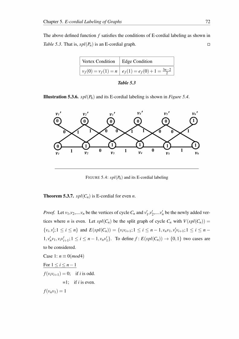
Chapter 5. E-cordial Labeling of Graphs 72
The above defined function f satisfies the conditions of E-cordial labeling as shown in
Table 5.3. That is, spl(Pn) is an E-cordial graph. �
Vertex Condition Edge Condition
v f (0) = v f (1) = n e f (1) = e f (0)+1 = 3n−22
Table 5.3
Illustration 5.3.6. spl(P6) and its E-cordial labeling is shown in Figure 5.4.
v1 v2 v3 v4 v5 v6
v1' v2' v3' v4' v5' v6'
0 0 0 0 0
0 0
0 0 0 0 0
0
1
1 1 1 1 1
1 1 1 1 11 1 1
FIGURE 5.4: spl(P6) and its E-cordial labeling
Theorem 5.3.7. spl(Cn) is E-cordial for even n.
Proof. Let v1,v2,....vn be the vertices of cycle Cn and v′1,v′2,....v′n be the newly added ver-
tices where n is even. Let spl(Cn) be the split graph of cycle Cn with V (spl(Cn)) =
{vi,v′i;1 ≤ i ≤ n} and E(spl(Cn)) = {vivi+1;1 ≤ i ≤ n− 1,vnv1,v′ivi+1;1 ≤ i ≤ n−
1,v′nv1,viv′i+1;1 ≤ i ≤ n− 1,vnv′1}. To define f : E(spl(Cn))→ {0,1} two cases are
to be considered.
Case 1: n≡ 0(mod4)
For 1≤ i≤ n−1
f (vivi+1) = 0; if i is odd.
=1; if i is even.
f (vnv1) = 1
Chapter 5. E-cordial Labeling of Graphs 73
For 1≤ i≤ n−1
f (viv′i+1) = 0; if i≡ 1,2(mod4)
=1; if i≡ 0,3(mod4)
f (vnv′1) = 1
For 1≤ i≤ n−1
f (v′ivi+1) = 1; if i≡ 1,2(mod4)
=0; if i≡ 0,3(mod4)
f (v′nv1) = 0.
Case 2: n≡ 2(mod4)
For 1≤ i≤ n−1
f (vivi+1) = 0; if i is odd.
=1; if i is even.
f (vnv1) = 0
For 1≤ i≤ n−1
f (viv′i+1) = 0; if i≡ 1,2(mod4)
=1; if i≡ 0,3(mod4)
f (vnv′1) = 1
For 1≤ i≤ n−1
f (v′ivi+1) = 1; if i≡ 1,2(mod4)
=0; if i≡ 0,3(mod4)
f (v′nv1) = 1.
In view of the above defined labeling pattern f satisfies the conditions for E-cordial
labeling as shown in Table 5.4. That is, the spl(Cn) for n is even is E-cordial. �
n Vertex Condition Edge Condition
n≡ 0,2(mod4) v f (0) = v f (1) = n e f (0) = e f (1) = 3n2
Table 5.4
Illustration 5.3.8. Figure 5.5 shows the E-cordial labeling of spl(C8).

Chapter 5. E-cordial Labeling of Graphs 74
v1
v2
v3
v4
v5
v6
v7
v8
v1'
v2'
v3'
v4'
v5'v6'
v7'
v8'
0
0
0
0
0 0
0
00
0
0
0
00
0
0
0
00
0
1 1
1
1
1
1
1
11
1
1
1
1
1
1
1
1
1
1
1
FIGURE 5.5: spl(C8) and its E-cordial labeling
Theorem 5.3.9. Pn[P2] is E-cordial when n is even.
Proof. Consider two copies of Pn. Let v1,v2,. . . , vn be the vertices of first copy of Pn
and u1,u2,. . . , un be the vertices of the second copy of Pn. Let G be Pn[P2]. V (G)=T1⋃
T2
where T1 = {(vi,u1),1≤ i≤ n} and T2 = {(vi,u2),1≤ i≤ n}, E(G)={(vi,u1)(vi+1,u1);1≤
i≤ n−1,(vi,u2)(vi+1,u1);1≤ i≤ n−1,(vi,u1)(vi+1,u2);1≤ i≤ n−1,(vi,u2)(vi+1,u1);1≤
i≤ n−1,(vi,u1)(vi,u2);1≤ i≤ n}. Define f : E(G)→{0,1} as follows.
For 1≤ i≤ n−1
f ((vi,u1)(vi+1,u1)) = 0; if i is odd.
= 1; if i is even.
For 1≤ i≤ n−1
f ((vi,u2)(vi+1,u2)) = 1; if i is odd.
= 0; if i is even.
For 1≤ i≤ n−1
f ((vi,u1)(vi+1,u2)) = 1; if i is odd.
= 0; if i is even.

Chapter 5. E-cordial Labeling of Graphs 75
For 1≤ i≤ n−1
f ((vi,u2)(vi+1,u1)) = 1; if i is odd.
= 0; if i is even.
For 1≤ i≤ n−1
f ((vi,u1)(vi,u2))= 0; if i is odd.
=1; if i is even.
f ((vn,u1)(vn,u2))= 0.
In view of the above defined labeling pattern f satisfies the conditions for E-cordial
labeling as shown in Table 5.5. That is, Pn[P2] is E-cordial when n is even. �
Vertex Condition Edge Condition
v f (0) = v f (1) = n e f (0) = e f (1) = 5n−42
Table 5.5
Illustration 5.3.10. In Figure 5.6 the graph P6[P2] and its E-cordial labeling is shown.
1
0
(v2,u1) (v3,u1) (v4,u1) (v5,u1) (v6,u1)
(v1,u2) (v2,u2) (v3,u2) (v4,u2) (v5,u2) (v6,u2)
1
(v1,u1)
0 0
000
0 0 0
0
00
00 0 0 0
0 0
1 1
111
1 1 1 1 1 1
1 1
1 1
1 1
FIGURE 5.6: P6[P2] and its E-cordial labeling
Theorem 5.3.11. The graph obtained by duplication of an arbitrary vertex of Cn admits
E-cordial labeling.
Proof. Let v1,v2,. . . , vn be the vertices of the cycle Cn. Let G be the graph obtained by
duplicating an arbitrary vertex of Cn. Without loss of generality let this vertex be v1 and

Chapter 5. E-cordial Labeling of Graphs 76
the newly added vertex be v′1. E(G)={E(Cn),e′,e′′} where e′ = v′1v2 and e′′ = vnv′1.To
define f : E(G))→{0,1} two cases are to be considered.
Case 1: n≡ 0,2(mod4)
f (e′) = 0
f (e′′) = 1
For 1≤ i≤ n
f (ei) = 0; for i≡ 1,0(mod4),
=1; for i≡ 2,3(mod4)
Case 2: n≡ 3(mod4)
f (e′) = 0
f (e′′) = 1
For 1≤ i≤ n
f (ei) = 1; for i≡ 1,2(mod4),
=0; for i≡ 0,3(mod4)
In view of the above defined labeling pattern f satisfies the conditions for E-cordial
labeling as shown in Table 5.6. That is, the graph obtained by the duplication of an
arbitrary vertex in cycle Cn admits E-cordial labeling. �
n vertex condition edge condition
n≡ 0(mod4) v f (0) = v f (1)+1 = n+22 e f (0) = e f (1) = n+2
2
n≡ 2(mod4) v f (1) = v f (0)+1 = n+22 e f (0) = e f (1) = n+2
2
n≡ 3(mod4) v f (1) = v f (0) = n+12 e f (1) = e f (0)+1 = n+3
2
Table 5.6
Illustration 5.3.12. Figure 5.7 shows the E-cordial labeling of the graph obtained by
the duplication of an arbitrary vertex in cycle C12.

Chapter 5. E-cordial Labeling of Graphs 77
v1
v1'
v2
v3
v4
v5
v6
v7
v8
v9
v10
v11
v12
e4
e5
e6e7
e8
e9
e10
e11
e12 e1
e2
e3
e'' e'0
00
00
0
0
0
0
0
0
00
0
1
1
1
1
1
1
11 1
1
1
1
1
FIGURE 5.7: The graph obtained by the duplication of an arbitrary vertex in cycle C12and its E-cordial labeling
Theorem 5.3.13. The graph obtained by duplication of an arbitrary edge in Cn admits
E-cordial labeling.
Proof. Let v1,v2,. . . , vn be the vertices of the cycle Cn. Let G be the graph obtained by
duplicating an arbitrary edge of Cn. Without loss of generality let this edge be e1 = v1v2
and the newly added edge be e′1 = v′1v′2. E(G)={E(Cn),e′1,e′,e′′} where e′ = v′2v3 and
e′′ = vnv′1. Define f : E(G)→{0,1} as follows.
Case 1: n≡ 1,2(mod4)
f (e′1) = 1
f (e′) = 0
f (e′′) = 1
For 1≤ i≤ n
f (ei) = 0; for i≡ 0,1(mod4),
=1; for i≡ 2,3(mod4)

Chapter 5. E-cordial Labeling of Graphs 78
Case 2: n≡ 3(mod4)
f (e′1) = 1
f (e′) = 0
f (e′′) = 1
For1≤ i≤ n−1
f (ei) = 0; for i≡ 0,1(mod4),
=1; for i≡ 2,3(mod4)
f (en) = 0.
In view of the above defined labeling pattern f satisfies the conditions for E-cordial
labeling as shown in Table 5.7. That is, the graph obtained by the duplication of an
arbitrary edge in cycle Cn is E-cordial. �
n vertex condition edge condition
n≡ 1(mod4) v f (1) = v f (0)+1 = n+32 e f (0) = e f (1) = n+3
2
n≡ 2(mod4) v f (1) = v f (0) = n+22 e f (1) = e f (0)+1 = n+4
2
n≡ 3(mod4) v f (0) = v f (1)+1 = n+32 e f (0) = e f (1) = n+3
2
Table 5.7
Illustration 5.3.14. The E-cordial labeling of the graph obtained by the duplication of
an arbitrary edge in cycle C11 is as shown in Figure 5.8.
v1 v2
v1' v2'
v3
v4
v5
v6
v7
v8
v9
v10
v11
e1
e2
e3
e4
e5
e6e7
e8
e9
e10
e11
e'' e'
e1'
0
0
00
0
0
0
0
0
0
0
0
11
1
1
1
11
1
1
0 1
1
11
0
FIGURE 5.8: The graph obtained by the duplication of an arbitrary edge in cycle C11and its E-cordial labeling

Chapter 5. E-cordial Labeling of Graphs 79
Theorem 5.3.15. Joint sum of two copies of Cn of even order produces an E-cordial
graph.
Proof. We denote the vertices of first copy of Cn by v1,v2,....vn and second copy by v′1,
v′2,v′3,....v′n, ei and e′i where 1 ≤ i ≤ n be the corresponding edges. Join the two copies
of Cn with a new edge and let G be the resultant graph. Without loss of generality we
assume that the new edge be e=v1v′1. To define f : E(G)→ {0,1} two cases are to be
considered.
Case 1: n≡ 0(mod4)
f (e) = 0
For 1≤ i≤ n
f (ei) = 0; for i≡ 0,1(mod4),
=1; for i≡ 2,3(mod4)
For 1≤ i≤ n
f (e′i) = 0; for i≡ 0,1(mod4),
=1; for i≡ 2,3(mod4)
Case 2: n≡ 2(mod4)
f (e) = 1
For 1≤ i≤ n
f (ei) = 0; for i≡ 0,1(mod4),
=1; for i≡ 2,3(mod4)
For 1≤ i≤ n
f (e′i) = 0; for i≡ 0,1(mod4),
=1; for i≡ 2,3(mod4)
In view of the above defined labeling pattern f satisfies the conditions for E-cordial
labeling as shown in Table 5.8. That is, the joint sum of two copies of even cycle Cn is
E-cordial. �
n Vertex Condition Edge Condition
n≡ 0(mod4) v f (0) = v f (1) = n e f (0) = e f (1)+1 = n+1
n≡ 2(mod4) v f (0) = v f (1) = n e f (1) = e f (0)+1 = n+1
Table 5.8

Chapter 5. E-cordial Labeling of Graphs 80
Illustration 5.3.16. E-cordial labeling of joint sum of two copies of cycle C10 is shown
in Figure 5.9.
v1
v2
v3
v4
v5
v6
v7
v8
v9
v10
v1'
v2'
v3'
v4'
v5'
v6'v7'
v8'
v9'
v10'
e1
e2
e3
e4
e5e6
e7
e8
e9
e10
e
e1'
e2'
e3'
e4'
e5'e6'
e7'
e8'
e9'
e10'0 0
0
00
0 0
00
0
0
0
0
0
0
0
0
0
0
0
1
1
1
1
1
1
1
1 1
1
1
1
1
1
1
1
1
11
1
1
FIGURE 5.9: The joint sum of two copies of cycle C10 and its E-cordial labeling
Theorem 5.3.17. D2(Pn) is E-cordial when n is even.
Proof. Let P′n P′′n be two copies of path Pn. We denote the vertices of first copy of Pn
by v′1,v′2,....v′n and second copy by v′′1 , v′′2 ,....v′′n . Let G be D2(Pn) with |v(G)| = 2n and
|E(G)|= 4n−4. To define f : E(G)→{0,1} two cases are to be considered.
Case 1: n≡ 0(mod4)
For 1≤ i≤ n−1
f (v′iv′i+1) = 1; if i , 3 j
=0; if i = 3 j, j = 1,2, . . .bn3c
For 1≤ i≤ n−1
f (v′′i v′′i+1) = 0; if i , 3 j
=1; if i = 3 j, j = 1,2, . . .bn3c
For 1≤ i≤ n−2
f (v′′i v′i+1) = 1; if i is odd.
=0; if i is even.
f (v′′n−1v′n) = 0

Chapter 5. E-cordial Labeling of Graphs 81
For 1≤ i≤ n−1
f (v′iv′′i+1) = 1; if i is odd.
=0; if i is even.
Case 2: n≡ 2(mod4)
For 1≤ i≤ n−1
f (v′iv′i+1) = 1; if i≡ 1,2(mod4)
=0; if i≡ 0,3(mod4)
For 1≤ i≤ n−1
f (v′′i v′′i+1) = 0; if i≡ 1,2(mod4)
=1; if i≡ 0,3(mod4)
For 1≤ i≤ n−2
f (v′iv′′i+1) = 1; if i is odd.
=0; if i is even.
f (v′n−1v′′n) = 0
For 1≤ i≤ n−1
f (v′′i v′i+1) = 1; if i is odd.
=0; if i is even.
In view of the above defined labeling pattern f satisfies the conditions for E-cordial
labeling as shown in Table 5.9. That is, D2(Pn) where n is even is E-cordial. �
n Vertex Condition Edge Condition
n≡ 0,2(mod4) v f (0) = v f (1) = n e f (0) = e f (1) = 2n−2
Table 5.9
Illustration 5.3.18. Figure 5.10 shows the E-cordial labeling of D2(P6).

Chapter 5. E-cordial Labeling of Graphs 82
v1' v2' v3' v4' v5' v6'
v1'' v2'' v3'' v4'' v5'' v6''0 0
0 0
0 0 0 0 0
1 1 11 1 1
1 1 1
1 1 1 1 1
0 0 0 0
000
1 1
FIGURE 5.10: D2(P6) and its E-cordial labeling
5.4 Concluding Remarks and Further Scope of Research
Nine new results have been investigated on E-cordial labeling. To derive similar
results for various labeling problems and for different graph families is an open area of
research.
The next chapter is targeted to discuss odd sequential labeling of graphs.
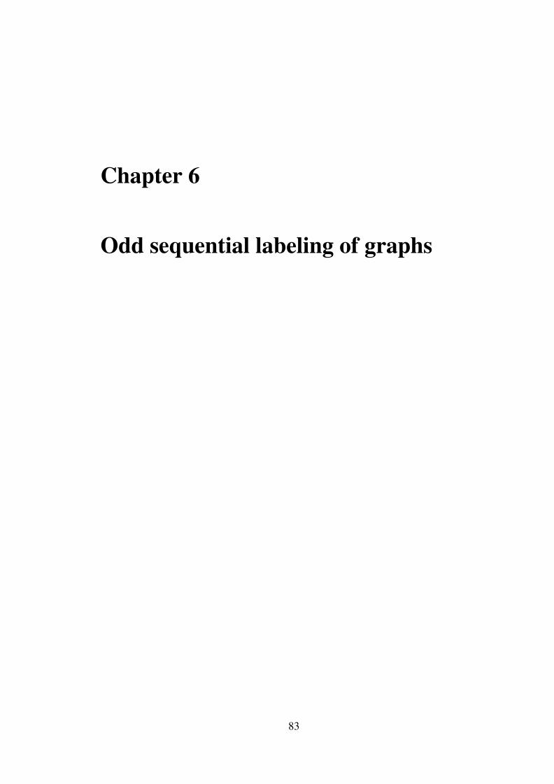
Chapter 6
Odd sequential labeling of graphs
83

Chapter 6. Odd sequential labeling of graphs 84
6.1 Introduction
This chapter is intended to discuss odd sequential labeling of graphs. Here we
investigate nine results on odd sequential labeling as well as we introduce two new con-
cepts namely bi-odd sequential graphs and global odd sequential graphs.
6.2 Sequential labeling
A graph G=(V(G),E(G)) with p vertices and q edges is said to be strongly c-harmonious
if f : V (G)→{0,1,2, . . . ,q−1} is injective and the induced function f* : E(G)→{c,c+
1,c+2, . . . ,c+q−1} defined as f*(e = uv) = f (u)+ f (v) is bijective.
Chang et al.[7] have introduced strongly c-harmonious labeling. But Grace [21] called
such a labeling sequential. We continue with Grace’s terminology.
The graph which admits sequential labeling is called a sequential graph.
6.3 Odd Sequential labeling
A graph G = (V (G),E(G)) with p vertices and q edges is said to be an odd sequential
labeling if there is an injection f : V (G)→{0,1,2, . . . ,q} or if G is a tree then f : V (G)→
{0,1,2, . . . ,2q− 1} is an injection such that when each edge xy is assigned the label
f (x)+ f (y), the resulting edge labels are {1,3, . . . ,2q−1}.
The graph which admits odd sequential labeling is known as an odd sequential graph.
6.3.1 Illustration
K1,4 and its odd sequential labeling is shown in Figure 6.1.

Chapter 6. Odd sequential labeling of graphs 85
v1 v2 v3 v4
v
0
1 753
FIGURE 6.1: K1,4 and its odd sequential labeling
6.3.2 Some existing results
Singh and Varkey [40] have introduced the notion of odd sequential graphs and they
have proved that
• Combs are odd sequential graphs.
• Grids are odd sequential graphs.
• Stars are odd sequential graphs.
• Rooted trees of level 2 are odd sequential graphs.
• Odd cycles do not admit odd sequential labeling.
Balakrishnan et al.[1] have mentioned about the above defined labeling with a slight
variation as follows which they called an odd-edge labeling.
A 1-1 function f : V (G)→{0,1,2, . . . ,q} is said to be an odd-edge labeling of a graph G
if for any edge xy ∈ E(G), f ∗(xy) = f (x)+ f (y), the resulting edge labels are {1,3, . . . ,
2q−1} and the induced function f ∗ is one - one.
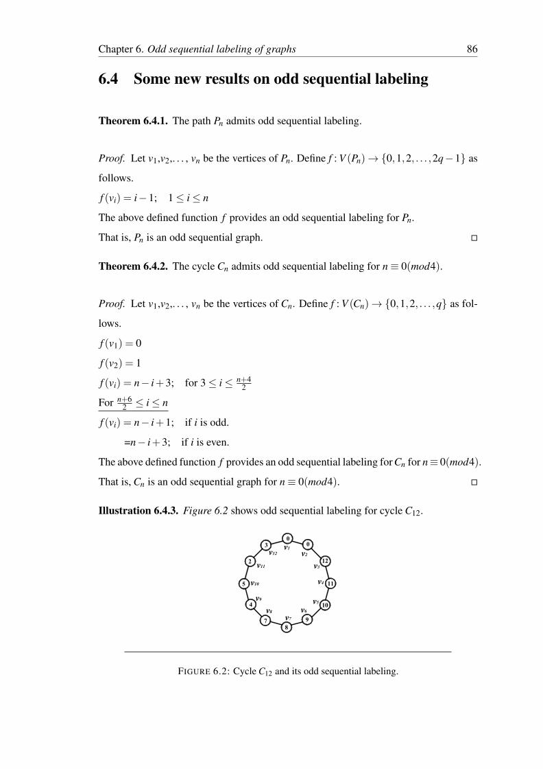
Chapter 6. Odd sequential labeling of graphs 86
6.4 Some new results on odd sequential labeling
Theorem 6.4.1. The path Pn admits odd sequential labeling.
Proof. Let v1,v2,. . . , vn be the vertices of Pn. Define f : V (Pn)→{0,1,2, . . . ,2q−1} as
follows.
f (vi) = i−1; 1≤ i≤ n
The above defined function f provides an odd sequential labeling for Pn.
That is, Pn is an odd sequential graph. �
Theorem 6.4.2. The cycle Cn admits odd sequential labeling for n≡ 0(mod4).
Proof. Let v1,v2,. . . , vn be the vertices of Cn. Define f : V (Cn)→ {0,1,2, . . . ,q} as fol-
lows.
f (v1) = 0
f (v2) = 1
f (vi) = n− i+3; for 3≤ i≤ n+42
For n+62 ≤ i≤ n
f (vi) = n− i+1; if i is odd.
=n− i+3; if i is even.
The above defined function f provides an odd sequential labeling for Cn for n≡ 0(mod4).
That is, Cn is an odd sequential graph for n≡ 0(mod4). �
Illustration 6.4.3. Figure 6.2 shows odd sequential labeling for cycle C12.
00
12
11
10
98
7
4
5
2
3 v1
v2
v3
v4
v5
v7
v8
v9
v10
v11
v12
v6
FIGURE 6.2: Cycle C12 and its odd sequential labeling.

Chapter 6. Odd sequential labeling of graphs 87
Theorem 6.4.4. The crown Cn�K1 is an odd sequential graph when n is even.
Proof. Let v1,v2,. . . , vn be the vertices of Cn where n is even. Let u1,u2,. . . , un be the
newly added pendant vertices and let G be Cn�K1. To define f : V (G)→{0,1,2, . . . ,q}
two cases are to be considered as follows.
Case 1:n≡ 0(mod4)
For 1≤ i≤ n2 +1
f (vi) = 2i−1; if i is odd.
=2i−2; if i is even.
For n2 +2≤ i≤ n
f (vi) = 2i; if i is even.
=2i−1; if i is odd.
For 1≤ i≤ n2
f (ui) = 2i−2; if i is odd.
=2i−1; if i is even.
For n2 +1≤ i≤ n
f (ui) = 2i; if i is odd.
=2i−1; if i is even.
Case 2:n≡ 2(mod4)
For 1≤ i≤ n2
f (vi) = 2i−2; if i is odd.
=2i−1; if i is even.
f (vi) = 2i+1; for n2 +1
For n+42 ≤ i≤ n
f (vi) = 2i; if i is odd.
=2i−1; if i is even.
For 1≤ i≤ n2 +1
f (ui) = 2i−1; if i is odd.
=2i−2; if i is even.
f (ui) = 2i−3; for n2 +2

Chapter 6. Odd sequential labeling of graphs 88
For n2 +3≤ i≤ n
f (vi) = 2i; if i is even.
=2i−1; if i is odd.
The above defined pattern covers all the possibilities and the graph under consideration
admits an odd sequential labeling.
That is,the crown Cn�K1 is an odd sequential graph when n is even. �
Illustration 6.4.5. The odd sequential labeling for C12�K1 is given in Figure 6.3.
0
1
3
2
5
4
6 7
9
810
11
13
1415
1618
17
19 20
22
21
23
24v1 v2
v3
v4
v5
v6
v7
v8
v9
v10
v11
v12
u1
u2
u3
u4
u5
u6
u7
u8
u9
u10
u11
u12
FIGURE 6.3: C12�K1 and its odd sequential labeling
Theorem 6.4.6. The graph obtained by duplication of an arbitrary vertex in even cycle
Cn admits odd sequential labeling.
Proof. Let v1,v2,. . . , vn be the vertices of Cn where n is even. Without loss of generality
assume that the vertex v1 is duplicated by a new vertex v′1. Let G be the resultant graph.
To define f : V (G)→{0,1,2, . . . ,q} two cases are to be considered as follows.
Case 1:n≡ 0(mod4)
f (v1) = 3
f (v′1) = 1
f (vi) = n− i+4; for 2≤ i≤ n2 +1

Chapter 6. Odd sequential labeling of graphs 89
For n2 +2≤ i≤ n
f (vi) = n− i; if i is even.
=n− i+4; if i is odd.
Case 2:n≡ 2(mod4)
f (v1) = 0
f (v′1) = 2
f (v2) = 1
f (vi) = n− i+5; for 3≤ i≤ n2 +3
For n2 +4≤ i≤ n
f (vi) = n− i+3; if i is odd.
=n− i+5; if i is even.
In both the cases the above described function f provides an odd sequential labeling for
the graph under consideration.
That is, the graph obtained by duplication of an arbitrary vertex in even cycle Cn admits
odd sequential labeling. �
Illustration 6.4.7. The odd sequential labeling for the graph obtained by the duplication
of an arbitrary vertex in cycle C12 is given in Figure 6.4.
0
1
3
5
2
7
49
10
11
12
13
14v1
v1'
v2
v3
v4
v5
v6v7
v8
v9
v10
v11
v12
FIGURE 6.4: The graph obtained by the duplication of an arbitrary vertex in cycle C12and its odd sequential labeling

Chapter 6. Odd sequential labeling of graphs 90
Theorem 6.4.8. S(Tn) is an odd sequential graph.
Proof. Let Pn be a path on n vertices denoted by (1,1),(1,2), . . . ,(1,n) and has n− 1
edges denoted by e1,e2, . . . ,en−1 where ei is the edge joining the vertices (1, i) and
(1, i+1). The step ladder graph S(Tn) has n2+3n−22 vertices denoted by (1,1),(1,2), . . . ,
(1,n),(2,1),(2,2), . . . ,(2,n),(3,1),(3,2), . . . ,(3,n−1),(4,1),(4,2), . . . ,(4,n−2), . . . ,
(n,1),(n,2). In the ordered pair (i, j), i denotes the row (counted from bottom to top)
and j denotes the column (from left to right) in which the vertex occurs. Define f :
V (S(Tn))→{0,1,2, . . . ,q} as follows.
f (i, j) = n2−2n(i−1)+ i(i−2)+ j−1; for 1≤ i, j ≤ n.
Then f provides an odd sequential labeling for S(Tn).
That is, S(Tn) is an odd sequential graph. �
Illustration 6.4.9. Figure 6.5 shows odd sequential labeling of S(T6).
(1,1) (1,2) (1,3) (1,4) (1,5) (1,6)
(2,1) (2,2) (2,3) (2,4) (2,5) (2,6)
(3,1) (3,2) (3,3) (3,4) (3,5)
(4,1) (4,2) (4,3) (4,4)
(5,1) (5,2) (5,3)
(6,1) (6,2)
40
29
39
28
38
27
36
25
35
24
15 16 17 18 19
1110
37
26
0 1
3 4 5
8 9
FIGURE 6.5: S(T6) and its odd sequential labeling

Chapter 6. Odd sequential labeling of graphs 91
Theorem 6.4.10. The path union of stars is an odd sequential graph.
Proof. Let v1,v2,. . . , vn be the vertices of Pn. Consider n copies of star K1,m and let
{vi j,1 ≤ i ≤ n,1 ≤ j ≤ m} be their corresponding pendant vertices. Let G be the path
union graph of n copies of star K1,m. Define f : V (G)→{0,1,2, . . . ,2q−1} as follows.
For 1≤ i≤ n
f (vi) = i(m+1)−1; if i is even.
=(i−1)(m+1); if i is odd.
For 1≤ i≤ n, 1≤ j ≤ m
f (vi j) = (i−1)(m+1)+2 j−1; if i is odd.
=i(m+1)−2(m− j+1); if i is even.
The above defined function f provides an odd sequential labeling for the path union of
stars.
That is, the path union of stars is an odd sequential graph. �
Illustration 6.4.11. Figure 6.6 shows odd sequential labeling for the path union of four
copies of star K1,4.
0 9
13 5
7 24 6
8
10 19
1113 15
17 1214 16
18
v1 v2 v3 v4
v11
v12 v13v14 v21
v23
v24
v22
v31
v32 v33
v34v41
v42 v43
v44
FIGURE 6.6: Path union of four copies of star K1,4 and its odd sequential labeling
Theorem 6.4.12. The graph 〈K(1)1,n : K(2)
1,n : . . . : K(m)1,n 〉 admits odd sequential labeling.
Proof. Consider m copies of stars K1,n and let G be the graph 〈K(1)1,n : K(2)
1,n : . . . : K(m)1,n 〉.
Let V (G) = {vi; i = 1,2, . . . ,m,vi j; i = 1,2, . . . ,m, j = 1,2, . . . ,n,xi; i = 1,2, . . . ,m− 1}
and E(G) = {vivi j; i = 1,2, . . . ,m, j = 1,2, . . . ,n,vixi; i = 1,2, . . . ,m−1,xivi+1; i = 1,2,
. . . ,m−1} so that |V (G) |=m(n+2)−1 and |E(G) |=m(n+2)−2. Define f : V (G)→

Chapter 6. Odd sequential labeling of graphs 92
{0,1,2, . . . ,2q−1} as follows.
f (vi) = 2i−2; 1≤ i≤ m
f (v1 j) = 2 j−1; 1≤ j ≤ n
f (vi j) = 2i(n+1)−2(n− j)−3; 2≤ i≤ m ;1≤ j ≤ n
f (xi) = 2i(n+1)−1; 1≤ i≤ m−1
The above defined function f provides an odd sequential labeling for the graph 〈K(1)1,n :
K(2)1,n : . . . : K(m)
1,n 〉.
That is, the graph 〈K(1)1,n : K(2)
1,n : . . . : K(m)1,n 〉 is an odd sequential graph. �
Illustration 6.4.13. Figure 6.7 shows odd sequential labeling for the graph 〈K(1)1,4 : K(2)
1,4 :
K(3)1,4 〉.
v1 v2 v3x1 x2
v11v12 v13 v14
v21v22 v23 v24 v31
v32 v33v34
0
13 5 7
9 2 4
1113 15
17
19
2123 25
27
FIGURE 6.7: The graph 〈K(1)1,4 : K(2)
1,4 : K(3)1,4 〉 and its odd sequential labeling
Theorem 6.4.14. SS(Pn) admits odd sequential labeling.
Proof. Let Pn be the path containing n vertices v1,v2,. . . ,vn and n− 1 edges. Let ei
denotes the edge vivi+1 in Pn. For 1 ≤ i ≤ n− 1 each edge ei of path Pn is replaced by
a complete bipartite graph K2,mi where mi is any positive integer. Let ui j be the vertices
of the mi vertices part of the K2,mi where 1 ≤ i ≤ n− 1 and 1 ≤ j ≤ max{mi}. Define
f : V (SS(Pn))→{0,1,2, . . . ,q} as follows.
f (v1) = 0
f (vi) = 2i−1
∑k=1
mk; 2≤ i≤ n
f (u1 j) = 2 j−1; 1≤ j ≤ m1
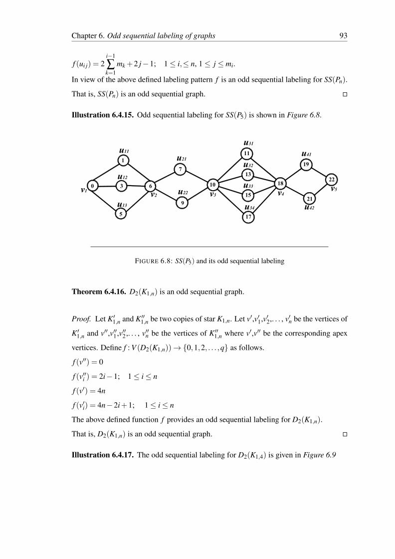
Chapter 6. Odd sequential labeling of graphs 93
f (ui j) = 2i−1
∑k=1
mk +2 j−1; 1≤ i,≤ n, 1≤ j ≤ mi.
In view of the above defined labeling pattern f is an odd sequential labeling for SS(Pn).
That is, SS(Pn) is an odd sequential graph. �
Illustration 6.4.15. Odd sequential labeling for SS(P5) is shown in Figure 6.8.
0
1
3
5
6v1 v2 v3 v4
u11
u12
u13
u21
u22
u31
u32
u33
u34
u41
u42
v5
7
9
10
11
13
15
17
18
19
21
22
FIGURE 6.8: SS(P5) and its odd sequential labeling
Theorem 6.4.16. D2(K1,n) is an odd sequential graph.
Proof. Let K′1,n and K′′1,n be two copies of star K1,n. Let v′,v′1,v′2,. . . , v′n be the vertices of
K′1,n and v′′,v′′1 ,v′′2 ,. . . , v′′n be the vertices of K′′1,n where v′,v′′ be the corresponding apex
vertices. Define f : V (D2(K1,n))→{0,1,2, . . . ,q} as follows.
f (v′′) = 0
f (v′′i ) = 2i−1; 1≤ i≤ n
f (v′) = 4n
f (v′i) = 4n−2i+1; 1≤ i≤ n
The above defined function f provides an odd sequential labeling for D2(K1,n).
That is, D2(K1,n) is an odd sequential graph. �
Illustration 6.4.17. The odd sequential labeling for D2(K1,4) is given in Figure 6.9

Chapter 6. Odd sequential labeling of graphs 94
0
1 3 5 7
16
15 13 11 9
v1'' v2'' v3''
v1' v2' v3' v4'
v''
v'
v4''
FIGURE 6.9: D2(K1,4) and its odd sequential labeling
6.5 Bi-odd sequential and Global odd sequential graphs
We introduce the following two new concepts.
Definition 6.5.1. If a graph G and its line graph L(G) admit odd sequential labeling
then G is known as a bi-odd sequential graph.
Theorem 6.5.2. A disconnected graph can not be an odd sequential graph.
Proof. Let G be a disconnected graph with p vertices and q edges. According to basic
graph theory, a graph is disconnected when p≥ q+2. That is, if the number of vertices
is at least 2 more than the number of edges then G is disconnected. But in the odd
sequential labeling the vertex labels are only 0,1,2, . . .q. Hence a disconnected graph
can not be odd sequential. �
Theorem 6.5.3. The path Pn for all n and the cycle Cn for n ≡ 0(mod4) are bi-odd
sequential graphs.
Proof. L(Pn) and L(Cn) are isomorphic to Pn and Cn and we have already proved re-
spectively in Theorem 6.4.1 and Theorem 6.4.2 that paths Pn ∀n and cycle Cn for

Chapter 6. Odd sequential labeling of graphs 95
n ≡ 0(mod4) admit odd sequential labeling. Hence both of these graphs are bi-odd
sequential. �
Theorem 6.5.4. No trees except Pn is a bi-odd sequential graph.
Proof. Since all other trees with p ≥ 4 except Pn contains at least one K1,3 as a sub
graph and L(K1,3) is C3 which is a forbidden subgraph for an odd sequential graph as
proved by Singh and Varkey [40]. Hence path Pn is the only member in the family of
trees which is a bi-odd sequential graph. �
Definition 6.5.5. If a graph G and its compliment Gc admit odd sequential labeling then
G is known as a global odd sequential graph.
Theorem 6.5.6. No graph with p≥ 6 can be a global odd sequential graph.
Proof. According to Ramsey theory if G is a graph with p≥ 6, then either G or Gc con-
tains a triangle. Since all the odd cycles are forbidden subgraphs for an odd sequential
graph, a graph with p≥ 6 can not be a global odd sequential graph. �
Theorem 6.5.7. P4 is the only global odd sequential graph.
Proof. Consider any graph G with p < 6 and is odd sequential. Then Gc will either be
a disconnected graph or a graph contains C3 except for P4. As P4 being a self compli-
mentary graph it is the only global odd sequential graph. �
6.6 Concluding Remarks and Further Scope of Research
This chapter was targeted to discuss odd sequential labeling. In this chapter nine
new results on odd sequential labeling as well as two new concepts have been investi-
gated. To derive similar results for various labeling problems and for different graph
families is an open area of research.
Bibliography
[1] R Balakrishnan and A S V Yegnanarayanan, Indian J. pure appl.Math., (28), ,
905–916.
[2] C Barrientos, Odd-graceful labelings, Preprint.
[3] J C Bermond, Graceful graphs, Radio antennae and French windmills, Graph The-
ory and Combinatorics, Pitman, London, (1979), 18–37.
[4] G S Bloom and S W Golomb, Applications of numbered undirected graphs, Pro-
ceedings of IEEE, 165(4), (1977), 562–570.
[5] C Bu and C Cao, The gracefulness for a class of disconnected graphs, J. Natural
Sci.Heilongjiang Univ., 12, (1995), 6–8.
[6] I Cahit, Cordial graphs: a weaker version of graceful and harmonious graphs, Ars
Combin, 23, (1987), 201–207.
[7] G J Chang, D F Hsu and D G Rogers, Additive variations on a graceful
theme:Some results on harmonius and other related graphs, Congr. Numer., 32,
(1981), 181–197.
[8] P D Chawathe and V Krishna, Odd graceful labeling of contably infinite locally
finite bipartite graphs, Conference on Graph Theory and its Applications.
[9] W C Chen, H I Lu and Y N Yeh, Operations of interlaced trees and graceful trees,
Southeast Asian Bull. Math., 21, (1997), 337–348.
[10] J Clark and D A Holton, A first look at graph theory, Allied Publishers Ltd. (1995).
96

References 97
[11] C Delorme, M Maheo, H Thuillier, K M Koh and H K Teo, Cycles with a chord
are graceful, J. Graph Theory, 4, (1980), 409–415.
[12] J Devaraj, On edge-cordial graphs, Graph Theory notes of New york, XLVII,
(2004), 14–18.
[13] A Drake and T A Redl, On the enumeration of a class of non-graceful graphs,
Congressus Numerantium, 183, (2006), 175–184.
[14] P Eldergill, Decomposition of the Complete Graph with an Even Number of Ver-
tices, M.Sc Thesis, McMaster University.
[15] R Frucht, Graceful numbering of wheels and related graphs, Ann. N. Y. Acad. Sci.,
319, (1979), 219–229.
[16] R Frucht and J A Gallian, Labeling prisms, Ars Combin., 26, (1988), 69–82.
[17] J A Gallian, A dynamic survey of graph labeling, vol. 17 (2010).
[18] R B Gnanajothi, Topics in Graph Theory, Ph.D.Thesis, Madurai Kamraj Univer-
sity.
[19] C G Goh and C K Lim, Graceful numberings of cycles with consecutive chords,
(Unpublished).
[20] S W Golomb, How to number a graph, in: Graph Theory and Computing (edited
by R C Read), Academic Press, New York (1972), 23–37.
[21] T grace, On sequential labelings of graphs, J. Graph theory, 7, (1983), 195–201.
[22] J Gross and J Yellen, Graph theory and its applications, CRC press (1999).
[23] F Harary, Graph theory, Addison-Wesley, Reading, Massachusetts (1969).
[24] C Hoede and H Kuiper, All wheels are graceful, Util. Math., 14, (1987), 311.
[25] V J Kaneria, S K Vaidya, G V Ghodasara and S Srivastav, Some classes of dis-
connected graceful graphs, in: Proceedings of the first International confrence on
emerging technologies and applications in engineering, technology and sciences
on 13-14 Jan 2008 (edited by N N Jani and G R Kulkarni) (2008), 1050–1056.

References 98
[26] Q D Kang, Z H Liang, Y Z Gao and G H Yang, On the labeling of some graphs,
J. Combin. Math. Combin. Comput., 22, (1996), 193–210.
[27] K Kathiresan, Subdivisions of ladders are graceful, Indian J. pure appl. Math.,
23(1), (1992), 21–23.
[28] K Kathiresan, Some Classes of Odd graceful graphs, Anjac J. of Sciences, 7,
(2008), 5–10.
[29] K M Koh and N Punnim, On graceful graphs: cycle with 3 consecutive chords,
Bull. Malaysian Math. Soc., 5, (1982), 49–63.
[30] K M Koh, D G Rogers, H K Teo and K Y Yap, Graceful graphs: some further
results and problems, Congr. Numer., 29, (1980), 559–571.
[31] K M Koh and K Y Yap, Graceful numberings of cycles with a P3− chord, Bull.
Inst. Math. Acad. Sinica, 12, (1985), 41–48.
[32] S Lo, On edge graceful labelings of graphs, Congr. Numer., 50, (1985), 231–241.
[33] K J Ma and C J Feng, On the gracefulness of gear graphs, Math. Practice Theory,
(1984), 72–73.
[34] N Punnim and N Pabhapote, On graceful graphs: cycles with a Pk-chord, k ≥ 4,
Ars Combin., 23A, (1987), 225–228.
[35] G Ringel, Problem 25, in: Theory of graphs and its applications, proc. of sympo-
sium smolenice 1963, Prague, (1964), 162.
[36] A Rosa, On certain valuation of the vertices of a graph, Theory of graphs (Internat.
Symposium, Rome, July 1966), (1967), 349–355.
[37] C Sekar, Studies in Graph Theory, P.hD Thesis, Madurai Kamaraj University.
[38] M A Seoud, A T Diab and E A Elsahawi, On strongly C-harmonious, relatively
prime, odd graceful and cordial graphs, Proc. Math. Phys.Soc.Egypt, 73, (1998),
33–35.
References 99
[39] G Sethuraman and P Selvaraju, Gracefulness of arbitrary supersubdivisions of
graphs, Indian J. pure appl. Math., 32(7), (2001), 1059–1064.
[40] G S Singh and T K M Varkey, On odd sequential and bisequential graphs, Preprint.
[41] S Somasundaram and R Ponraj, Non existance of mean labeling for a wheel, Bul-
letin of Pure and Applied Sciences, 22E, (2003), 103–111.
[42] S Somasundaram and R Ponraj, Some results on mean graphs, Pure and applied
Mathematical Sciences, 58, (2003), 29–35.
[43] S Somasundaram and R Ponraj, On mean graphs of order < 5, J. of Decision and
Mathematical Sciences, 9, (2004), 47–58.
[44] M Truszczynski, Graceful unicyclic graphs, Demonstatio Mathematica, 17,
(1984), 377–387.
[45] S K Vaidya and K K Kanani, International journal of Information Science and
Computer Mathematics, (1), , 73–80.
[46] S K Vaidya, V J Kaneria, S Srivastav and N A Dani, Gracefulness of union of
two path graphs with grid graph and complete bipartite graph, in: Proceedings
of the first International confrence on emerging technologies and applications in
engineering, technology and sciences on 13-14 Jan 2008 (edited by N N Jani and
G R Kulkarni) (2008), 616–619.
[47] S K Vaidya and N B Vyas, International journal of Compt.Ad.Math., (2), , 22–27.
[48] D B West, Introduction to graph theory, 2nd ed., Prentice-Hall of India Pvt Ltd
(2006).
[49] R Yilmaz and I Cahit, E-cordial Graphs, Ars Combin., 46, (1997), 251–256.

List of Symbols
|B| Cardinality of set B.
Cn Cycle with n vertices.
Gc Compliment of a graph G.
Cn⊙
K1 Crown graph.
C(k)n One point union of k copies of Cycle Cn.
D2(G) Shadow graph of G.
diam(G) Diameter of G.
E(G) or E Edge set of graph G.
e f (n) Number of edges with edge label n.
fn Fan on n vertices.
Fn Friendship graph with 2n+1 vertices.
G = (V (G),E(G)) A graph G with vertex set V (G) and edge set E(G).
G1[G2] Composition of G1 and G2.
Kn Complete graph on n vertices.
Km,n Complete bipartite graph.
K1,n Star graph.
M(G) Middle graph of G
N(v) Open neighbourhood of vertex v.
N[v] Closed neighbourhood of vertex v.
Pn Path graph on n vertices.
spl(G) Split graph.
T (n, l) Tadpole graph.
T (G) Total graph of G.
100

List of Symbols 101
G1(T p)G2 Tensor Product of graphs G1 and G2.
SS(G) Arbitrary supersubdivision of G.
S(Tn) Step ladder graph.
V (G) or V Vertex set of graphs G.
v f (n) Number of vertices with vertex label n.
Wn Wheel on n vertices.
bnc Greatest integer not greater than real number n (Floor of n).

Annexure
102

1
International Journal of Algorithms, Computing and Mathematics
Volume 3, Number 1, February 2010
ns
Mean Labeling in the Context of Some Graph Operations
S K Vaidya
Department of Mathematics, Saurashtra University
Rajkot-360005, GUJARAT (INDIA)
Lekha Bijukumar Department of Mathematics, Saurashtra University
Rajkot-360005, GUJARAT (INDIA)
Abstract
In this paper we contribute some new results for mean labeling of graphs. We prove that
the graphs obtained by duplicating arbitrary vertex as well as an arbitrary edge in cycle
nC and the joint sum of two copies of nC admit mean labeling. We also prove that by
fusion of two vertices iv and jv in cycle nC with ( , ) 3i jd v v produce a mean graphs.
Key words: Mean labeling; Mean graph; Joint sum
AMS Subject Classification: 05C78
1. Introduction
We begin with simple, finite and undirected graph ( , )G V E with p vertices and q edges. In this
paper nC denotes the cycle with n vertices. For all other terminology and notations we follow
Harary [1]. For a detailed survey on graph labeling we refer to Gallian [2]. According to Beineke
and Hegde [3] graph labeling serves as a frontier between number theory and structure of graphs.
The definitions which are useful for the present investigation are given below.
Definition 1.1: If the vertices are assigned values subject to certain conditions then it is known
as graph labeling.
Definition 1.2: A function f is called a mean labeling of a graph ( , )G V E if
: {0,1,2, , }f V q is injective and the induced function *: {1,2, , }f E q
defined as
*( )f e uv ( ) ( )
2
f u f v if ( ) ( )f u f v is even
( ) ( ) 1
2
f u f v if ( ) ( )f u f v is odd

International Journal of Algorithms, Computing and Mathematics
2
is bijective. A graph which admits mean labeling is called a mean graph.
Definition 1.3: Consider two copies of nC , connect a vertex of first copy to a vertex of second
copy with a new edge, the new graph obtained is called joint sum of nC .
The mean labeling was introduced by Somasundaram and Ponraj[4] and the graphs
1,, , , ,
n n n m n m nP C K P P P C and the like are proved to be mean graphs. In [5] the same authors
proved that the subdivision graph of star 1,nK for 4n admits mean labeling. In [6] they also
proved that the wheel graph nW is not a mean graph for 3n . In this paper we contribute four
results for mean labeling in the context of some graphs operations.
2. Main Results.
Theorem 2.1: The graph obtained by duplicating an arbitrary vertex of cycle nC admits mean
labeling.
Proof: Let 1 2, , , nv v v be the vertices of the cycle nC . Let G be the resultant graph obtained by
duplicating an arbitrary vertex of nC . Without loss of generality let the vertex be 1v and the
duplicated vertex be 1v .To define : {0,1,2, , }f V q the following two cases are to be
considered.
Case 1: n is even.
We define the labeling as follows.
1( ) 1f v
1( ) 4f v
( ) 0nf v
( ) 2( 1)if v i , if 22
ni
( ) 2( ) 3if v n i , if 1 ( 1)2
ni n
Case 2: n is odd.
We define the labeling as follows.
1
1
2
( ) 0
( ) 5
( ) 4
( ) 1n
f v
f v
f v
f v
( ) 2 1if v i , if 1
32
ni
( ) 2( 2)if v n i , if 3
12
ni n

Mean Labeling in the Context of Some Graph Operations
3
Hence f is a mean labeling of the graph G. Thus the graph obtained by duplicating an arbitrary
vertex is a mean graph.
Illustration 2.2: Consider the graph G obtained by duplicating the vertex 1v of the cycle 6C .
The labeling is as shown in Figure1.
Figure 1. Duplication of a vertex in C6 and Mean Labeling
Theorem 2.3: The graph obtained by duplicating an arbitrary edge in cycle nC is a mean graph.
Proof: Let 1, 2 , , nv v v be the vertices of cycle. Let G be the resultant graph obtained by
duplicating an arbitrary edge of nC . Without loss of generality let this edge be 1 2e v v and the
duplicated edge be 1 2'e v v .To define : {0,1,2, , }f V q , we consider the following two
cases.
Case 1: n is even.
We define the labeling as follows.
1 2( ) 1; ( ) 0f v f v
1 2( ) 3; ( ) 2f v n f v n
( ) ( 4)if v n i , if 3 12
ni
( ) 12
in
f v , if 22
ni
( ) 12
i
nf v ; if 3
2
ni
( ) ( 2)if v n i ; if 42
ni
Case 2: n is odd.
We define the labeling as follows.
1 2( ) 1, ( ) 0f v f v
1( ) 3,f v n 2( ) 2f v n
1 4
6
8
7
5
0
v 1
v 2
v 3
v 4
v 5
v 6
' v 1

International Journal of Algorithms, Computing and Mathematics
4
( ) ( 4)if v n i ; if 3
32
ni
1( )
2i
nf v ; if
5
2
ni
3( )
2i
nf v ; if
7
2
ni
For ( ) 2if v n i ; if 9
2
ni
In view of the above defined labeling pattern G admits mean labeling, that is the graph obtained
by duplicating an arbitrary edge in cycle nC is a mean graph.
Illustration 2.4: Consider the graph G obtained by duplicating the edge 1 2v v of the cycle 9C .
The labeling is shown in Figure 2.
Figure 2. Duplication of an edge in Cn and Mean Labeling
Theorem 2.5: The joint sum of two copies of nC admits mean labeling.
Proof: We denote the vertices of first copy of nC by 1 2, , , nv v v and the second copy of nC
by 1 2 2, , ,n n nv v v . Let G be the resultant graph obtained by joining an arbitrary vertex of the
first copy of nC to an arbitrary vertex of the second copy of nC with a new edge. Let this new
edge be 1n nv v so that , ,1 2 1 2, , , ,n n nv v v v v forms a path in G. To define : {0,1,2, , }f V q
we consider two cases.
Case 1: n is even.
( ) 2if v i ; if 12
ni
( )if v n ; if 2
ni
( ) 2( ) 1if v n i ; if 1 12
ni n
( ) 0if v ; if i n
( ) 2 1if v n ; if 1i n
v 1 v
2
v 3
v 4
v 5
v 6
v 7
v 8
v 9
' v 1 ' v
2 1 0
10
9
8
7
5
3
2
12 11

Mean Labeling in the Context of Some Graph Operations
5
( ) 2(2 ) 4if v n i ; if 3
22
n i n
( ) 2( ) 1if v i n ; 3
12
i n
Case 2: n is odd.
( ) 2if v i ; if 1
12
ni
( )if v n ; if 1
2
ni
( ) 2( ) 1if v n i ; if 3
12
ni n
( ) 0if v ; if i n
( ) 2 1if v n ; if 1i n
( ) 2(2 ) 4if v n i ; if 3
2 ( 1)2
n i n
( ) 2( ) 1if v i n ; if 1
(3 5)2
i n
The above defined labeling pattern exhausts both the possibilities for n and in each case the
graph G is a mean graph.
Illustration 2.6: Consider the graph G which is the joint sum of two copies of 10C . The labeling
is given in the following Figure 3.
0
8
10
21
11
14
2
4
6
9
5
3 19
17
15
13
16
18
20
v10
v1
v2
v3
v5
v7
v8
v9
v11
v12
v13
v14
v15
v16
v17
v18
v19
v20
v4v
6
7
Figure 3. Joint sum of C10 and Mean Labeling
Theorem 2.7: Fusion of two vertices iv and jv when ,( ) 3i jd v v in cycle nC produces a mean
graph.

International Journal of Algorithms, Computing and Mathematics
6
Proof: we consider cycle nC with n vertices 1 2, , , nv v v .Let the vertex 1v be fused with kv and
the resultant graph be 1 { }n kG C v . To define 1: ( ) {0,1,2, , }f V G q consider the following
cases.
Case 1: 0(mod2)n and 0(mod2)k
We label the graph as follows.
1( ) 1f v k
( ) 2 22
i
kf v i ; if 2
2
ki
( ) 0if v ; if 12
ki
( ) 2 12
i
kf v i ; If 2 ( 1)
2
ki k
( ) 2 ( 1)if v i k ; ( 1)2
n kk i
( ) 2( ) ( 1)if v n i k ; If2
2
n ki
Case 2: 0(mod2)n and 1(mod2)k
We label the graph as follows.
1( ) 1f v k
1( ) 2 1
2i
kf v i ; if
12
2
ki
( ) 0if v ; if 1
2
ki
1( ) 2
2i
kf v i ; If
3( 1)
2
ki k
( ) 2 ( 1)if v i k ; If 1
( 1)2
n kk i
( ) 2( ) ( 2)if v n i k ; If 3
2
n ki
Case 3: 1(mod2)n and 0(mod2)k
We define the labeling as follows.
1( ) 1f v k
( ) 2 22
i
kf v i ; if
2
ki
( ) 0if v ; if 12
ki
( ) 2 1;2
i
kf v i if 2 1
2
ki k

Mean Labeling in the Context of Some Graph Operations
7
( ) 2 ( 1)if v i k ; 1
12
n kk i
( ) 2( ) ( 2)if v n i k ; if 3
2
n ki
Case 4: 1(mod2)n and 1(mod2)k
We define the labeling as follows.
1( ) 1f v k
1( ) 2 1
2i
kf v i ; if
12
2
ki
( ) 0if v ; if 1
2
ki
1
( ) 22
i
kf v i ; if
3( 1)
2
ki k
( ) 2 ( 1)if v i k ; if 2
( 1)2
n kk i
( ) 2( ) ( 2)if v n i k ; if 4
2
n ki
In all the four cases it is possible to assign labels in such a way that G1 admits mean labeling.
Illustration 2.8: Consider a graph G obtained by fusing two vertices 1v and 6v of cycle 11C .
This is the case when 1(mod2)n and 0(mod2)k .The mean labeling is shown in Figure 4.
Figure 4. Fusion of two vertices in C11 and Mean Labeling
References
[1] F.Harary, Graph theory , (Addison Wesley, Massachusetts). (1972).
[2] J A. Gallian,, “A dynamic survey of graph labeling” The Electronics J. of Combinatorics, 16( 2009),#DS6.
[3] L.W.Beineke and S.M.Hegde,“Strongly Multiplicative graphs”,Discuss. Math. Graph Theory 21(2001), 63-75.
[4] S.Somasundaram and R..Ponraj,“Some results on mean graphs”, Pure & Applied Mathematical Sciences,58
( 2003), 29-35.
0
5
7
9
11
10
8
3 4
2
v 1
v 2
v 3 v 4
v 5
v 7
v 8
v 9
v 10
v 11

International Journal of Algorithms, Computing and Mathematics
8
[5] S.Somasundaram and R.Ponraj ,“On mean graphs of order <5”, J. Decision and Mathematical Sciences,
9( 2004), 47-58.
[6] S.Somasundaram and R.Ponraj,“ Non–existence of mean labeling for wheel”, Bulletin of Pure and Applied
Sciences, 22e9(1)(2003),103-111.
[7] S.Somasundaram and R.Ponraj., “Mean labeling of graphs obtained by identifying two graphs”, Journal of
Discrete Mathematical Sciences and Cryptography, 11 (2) ( 2008), 239-252.
[8] M.A Seoud and M.A Salim, “On mean graphs”, Ars Combin., (To appear)
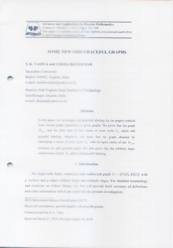


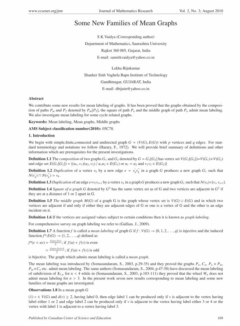
www.ccsenet.org/jmr Journal of Mathematics Research Vol. 2, No. 3; August 2010
Some New Families of Mean Graphs
S K Vaidya (Corresponding author)
Department of Mathematics, Saurashtra University
Rajkot 360 005, Gujarat, India
E-mail: [email protected]
Lekha Bijukumar
Shanker Sinh Vaghela Bapu Institute of Technology
Gandhinagar, GUJARAT, India
E-mail: [email protected]
Abstract
We contribute some new results for mean labeling of graphs. It has been proved that the graphs obtained by the composi-
tion of paths Pm and P2 denoted by Pm[P2], the square of path Pn and the middle graph of path Pn admit mean labeling.
We also investigate mean labeling for some cycle related graphs.
Keywords: Mean labeling, Mean graphs, Middle graphs
AMS Subject classification number(2010): 05C78.
1. Introduction
We begin with simple,finite,connected and undirected graph G = (V(G), E(G)) with p vertices and q edges. For stan-
dard terminology and notations we follow (Harary, F., 1972). We will provide brief summary of definitions and other
information which are prerequisites for the present investigations.
Definition 1.1 The composition of two graphs G1 and G2 denoted by G = G1[G2] has vertex set V(G1[G2])=V(G1)×V(G2)
and edge set E(G1[G2]) = {(u1, v1)(u2, v2) / u1u2 ∈ E(G1) or u1 = u2 and v1v2 ∈ E(G2)}Definition 1.2 Duplication of a vertex vk by a new edge e = v
′kv
′′k in a graph G produces a new graph G1 such that
N(v′k) ∩ N(v
′′k ) = vk.
Definition 1.3 Duplication of an edge e=vivi+1 by a vertex vk in a graph G produces a new graph G1 such that N(vk)={vi, vi+1}.Definition 1.4 Square of a graph G denoted by G2 has the same vertex set as of G and two vertices are adjacent in G2 if
they are at a distance of 1 or 2 apart in G.
Definition 1.5 The middle graph M(G) of a graph G is the graph whose vertex set is V(G) ∪ E(G) and in which two
vertices are adjacent if and only if either they are adjacent edges of G or one is a vertex of G and the other is an edge
incident on it.
Definition 1.6 If the vertices are assigned values subject to certain conditions then it is known as graph labeling.
For comprehensive survey on graph labeling we refer to (Gallian. J., 2009).
Definition 1.7 A function f is called a mean labeling of graph G if f : V(G) → {0, 1, 2, . . . , q} is injective and the induced
function f*:E(G) → {1, 2, . . . , q} defined as
f*(e = uv) =f (u)+ f (v)
2; if f (u) + f (v) is even
=f (u)+ f (v)+1
2; if f (u) + f (v) is odd
is bijective. The graph which admits mean labeling is called a mean graph.
The mean labeling was introduced by (Somasundaram, S., 2003, p.29-35) and they proved the graphs Pn, Cn, Pn × Pm,
Pm×Cn etc. admit mean labeling. The same authors (Somasundaram, S., 2004, p.47-58) have discussed the mean labeling
of subdivision of K1,n for n < 4 while in (Somasundaram, S., 2003, p.103-111) they proved that the wheel Wn does not
admit mean labeling for n > 3. In the present work seven new results corresponding to mean labeling and some new
families of mean graphs are investigated.
Observations 1.8 In a mean graph G
(1) v ∈ V(G) and d(v) ≥ 2, having label 0, then edge label 1 can be produced only if v is adjacent to the vertex having
label either 1 or 2 and edge label 2 can be produced only if v is adjacent to the vertex having label either 3 or 4 or the
vertex with label 1 is adjacent to a vertex having label 3.
Published by Canadian Center of Science and Education 169

www.ccsenet.org/jmr Journal of Mathematics Research Vol. 2, No. 3; August 2010
(2) The edge label q can be produced only when the vertices having labels q and q − 1 are adjacent in G.
2. Main Results
Theorem-2.1: The composition of paths Pm and P2 denoted as Pm[P2] admits mean labeling except for m = 2.
Proof: Let u1,u2,. . . , um be the vertices of the path Pm and v1,v2 be the vertices of path P2. The composition Pm[P2]
consists of 2m vertices, can be partitioned into two sets T1={(ui, v1),i = 1, 2, . . . ,m} and T2={(ui, v2),i = 1, 2, . . . ,m}. To
define f:V(G) → {0, 1, 2, . . . , q} following two cases are to be considered.
Case 1: m is even, m � 2
We define the labeling as follows.
f (u1, v1) = 0
f (u1, v2) = 2
f (u2, v1) = 4
f (u2, v2) = 7
For 3 ≤ i ≤ (m − 1)
f (ui, v1) = f (ui−1, v1) + 5; ∀i.
f (ui, v2) = f (ui−1, v2) + 6; when i is odd.
= f (ui−1, v2) + 4; when i is even
For i = m;
f (ui, v1) = f (ui−1, v1) + 6
f (ui, v2) = f (ui−1, v2) + 3
Case 2: m is odd.
We define the labeling as follows.
f (u1, v1) = 0
f (u1, v2) = 2
For 2 ≤ i ≤ m
f (ui, v1) = f (ui−1, v1) + 6; when i is odd.
= f (ui−1, v1) + 4; when i is even.
For 2 ≤ i ≤ (m − 1)
f (ui, v2) = f (ui−1, v2) + 6; when i is even.
= f (ui−1, v2) + 4; when i is odd.
For i = m;
f (ui, v1) = f (ui−1, v1) + 6
f (ui, v2) = f (ui−1, v2) + 3
In view of the above defined labeling pattern the graph under consideration admits mean labeling.
Case 3: m=2.
When m = 2 the resultant graph is K4 and as proved by (Somasundaram S., 2004, p.47-58) the complete graph Kn does
not admit mean labeling for n > 3.
Thus we conclude that the graph Pm[P2] admits mean labeling except for m = 2.
Remark:2.2
It is obvious from the observations 1.8 that the composition P2[Pm] does not admit mean labeling.
Illustration 2.3:
Consider the composition of P7 and P2. This is the case when n is odd. The mean labeling is as shown in Figure 1.
Theorem-2.4:The graph obtained by duplication of an arbitrary vertex by a new edge in cycle Cn admits mean labeling.
Proof: Let v1,v2,. . . , vn be the vertices of cycle Cn and let G be the graph obtained by duplicating an arbitrary vertex
170 ISSN 1916-9795 E-ISSN 1916-9809

www.ccsenet.org/jmr Journal of Mathematics Research Vol. 2, No. 3; August 2010
of Cn by a new edge. Without loss of generality let this vertex be v1 and the edge be e = v′1v′′1 . To define f : V(G) →{0, 1, 2, . . . , q} the following two cases are to be considered.
Case 1: n is odd.
We define the labeling as follows.
f (v1) = 3
f (v′1) = 0
f (v′′1) = 2
f (vi) = 2(i + 1); For 2 ≤ i ≤ ( n+12
)
f (vi) = 2(n + 3 − i) − 1; For n+32≤ i ≤ n
Case 2: n is even.
We define the labeling as follows.
f (v1) = 3
f (v′1) = 0
f (v′′1) = 2
f (vi) = 2(i + 1); For 2 ≤ i ≤ ( n2)
f (vi) = 2(n + 3 − i) − 1; For n+22≤ i ≤ n
Above defined labeling pattern exhaust all the possibilities and in each case the graph under consideration admits mean
labeling.
Illustration 2.5:
Consider the graph obtained by duplicating the vertex v1 by an edge v′1v′′1 in C8. This is the case when n is even.The
corresponding mean labeling is as shown in Figure 2.
Theorem-2.6: Duplication of an arbitrary edge by a new vertex in cycle Cn produces a mean graph.
Proof: Let v1,v2,. . . , vn be the vertices of cycle Cn. Let G be the graph obtained by duplication of an arbitrary edge in Cn by
a new vertex. Without loss of generality let this edge be e = v1v2 and the vertex be v′. To define f : V(G) → {0, 1, 2, . . . , q}the following two cases are to be considered.
Case 1: n is odd.
We define the labeling as follows.
f (v′) = 0
f (v1)=4
f (v2)=2
f (vi) = 2i; For 3 ≤ i ≤ ( n+12
)
f (vi) = 2(n + 2 − i) + 1; For n+32≤ i ≤ n
Case 2: n is odd.
We define the labeling as follows.
f (v′) = 0
f (v1) = 4
f (v2) = 2
f (vi) = 2i; For 3 ≤ i ≤ ( n+22
)
f (vi) = 2(n + 2 − i) + 1; For n+42≤ i ≤ n
In view of the above defined labeling pattern the graph under consideration admits mean labeling.
Illustration 2.7: Consider the graph obtained by duplicating an arbitrary edge v1v2 by a vertex v′ in cycle C9. This is the
case when n is odd. Labeling pattern is shown in Figure 3.
Theorem-2.8: P2n is a mean graph.
Published by Canadian Center of Science and Education 171

www.ccsenet.org/jmr Journal of Mathematics Research Vol. 2, No. 3; August 2010
Proof: Let v1,v2,....vn be the vertices of path Pn. Define f:V(G) → {0, 1, 2, . . . , q} as follows.
f (vi) = 2(i − 1); For i ≤ (n − 1)
f (vi) = 2i − 3; For i = n
Above defined labeling pattern provides mean labeling for P2n. i.e. P2
n is a mean graph.
Illustration 2.9:
The graph P29 and the corresponding mean labeling is shown in Figure 4.
Theorem-2.10: Crown (cycle with pendant edge attached at each vertex) is a mean graph.
Proof: Let v1,v2,. . . , vn be the vertices of cycle Cn. Let G1 be the crown with 2n vertices v1,v2,. . . , vn,u1,u2,. . . , un and 2nedges ( n edges of cycle Cn together with n pendant edges).
Case 1: n is odd.
we can label the graph as follows.
f (v1) = 0
f (u1) = 1
f (vi) = 2i − 1; For 2 ≤ i ≤ n+12
f (vi) = 2i; For n+32≤ i ≤ n
f (ui) = 2i − 2; For 2 ≤ i < n+12
f (ui) = 2i; For i = n+12
f (ui) = 2i − 1; For n+32≤ i ≤ n
Case 2: n is even.
we can label the graph as follows.
f (v1) = 0
f (u1) = 1
For 2 ≤ i ≤ n2
f (vi) = 2i − 1
f (ui) = 2i − 2
For n+22≤ i ≤ n;
f (vi) = 2i
f (ui) = 2i − 1
The above defined function f provides mean labeling for crown. i.e. crown is a mean graph.
Illustration 2.11 Consider the cycle C12 with 12 pendant vertices attached. This is the case when n is even. The mean
labeling pattern is as shown in Figure 5.
Theorem-2.12: Tadpoles T (n, k) (The graph obtained by identifying a vertex of cycle Cn to an end vertex of path Pk)
admits mean labeling.
Proof: Let v1,v2,. . . , vn be the vertices of cycle Cn and u1,u2,. . . , uk be the vertices of the path Pk. Let G1 be the resultant
graph obtained by identifying a vertex of cycle Cn to an end vertex of the path Pk. To define f:V(G) → {0, 1, 2, . . . , q} the
following two cases are to be considered.
Case 1: n is odd.
Identify one of the end vertices of Pk to a vertex of Cn in such a way that v n+32=u1. We can label the graph as follows.
f (vi) = 2(i − 1); For 1 ≤ i ≤ n+12
f (vi) = 2(n − i) + 3; For n+32≤ i ≤ n
f (u1) = f (v n+32
)
f (ui) = n + i − 1, i = 2, 3, . . . , k.
Case 2: n is even.
172 ISSN 1916-9795 E-ISSN 1916-9809

www.ccsenet.org/jmr Journal of Mathematics Research Vol. 2, No. 3; August 2010
Identify one of the end vertices of Pk to a vertex of Cn in such a way that v n+22=u1. We label the graph as follows.
f (vi) = 2(i − 1);For 1 ≤ i ≤ n+22
f (vi) = 2(n − i) + 3;For n+42≤ i ≤ n
f (u1) = f (v n+22
)
f (ui) = n + i − 1, i = 2, 3 . . . , k
In both the cases the above described function f provides mean labeling for the graph under consideration.
Illustration 2.13 In Figure 6 the graph T(9,4) and its mean labeling is shown.
Theorem-2.14: The middle graph of a path Pn denoted by M(Pn) admits mean labeling.
Proof: Let v1,v2,. . . vn be the vertices and e1,e2,. . . , en−1 be the edges of path Pn.The middle graph of a path Pn denoted by
M(Pn) is a graph with V[M(Pn)] = V(Pn)⋃
E(Pn) and two vertices are adjacent in M(Pn) if and only if they are adjacent
in Pn or one is a vertex and other is an incident edge to that vertex in Pn. M(Pn) consists of two types of vertices {v1,v2,. . . ,
vn} and {e1,e2,. . . , en−1}. To define f:V(M(Pn)) → {0, 1, 2, . . . , q} as follows.
f (e1) = 1
f (e2) = 4
f (e3) = 8
f (ei) = 3i − 1; 4 ≤ i ≤ (n − 1)
f (v1) = 0
f (vi) = 2i − 1; For 2 ≤ i ≤ 4
f (vi) = 3i − 5; For 5 ≤ i ≤ n
The above defined function f provides mean labeling for M(Pn). i.e. M(Pn) is a mean graph.
Illustration 2.15 The mean labeling for M(P6) is as shown in Figure 7 .
3. Concluding Remarks
We contribute here seven new results to the theory of mean graphs. This work is an effort to relate some graph operations
with mean labeling. We also introduce two concepts namely duplication of a vertex by an edge as well as duplication
of an edge by a vertex. We apply these operations to cycle Cn and prove that the resultant graphs are mean graphs. In
addition to this we prove that the middle graph of a path Pn admits mean labeling.
Future Scope:
It is possible to investigate similar results for other graph families and in the context of different labeling techniques.
References
Gallian, J. A. (2009). A dynamic survey of graph labeling, The Electronics Journal of Combinatorics, 16, �DS 6.
Harary, F. (1972). Graph Theory, Addison Wesley, Massachusetts.
Somasundaram, S. and Ponraj, R. (2003). Some results on mean graphs. Pure and Applied Mathematical Sciences, 58,
29-35.
Somasundaram, S. and Ponraj, R, (2004). On mean graphs of order < 5. J.Decision and Mathematical Sciences, 9, 47-58.
Somasundaram, S. and Ponraj, R. (2003). Non existence of mean labeling for wheel. Bulletin of Pure and AppliedSciences, 22E, 103-111.
Published by Canadian Center of Science and Education 173

www.ccsenet.org/jmr Journal of Mathematics Research Vol. 2, No. 3; August 2010
0 4 10 14 20 24 30
2 8 12 18 22 28 31
(u1,v1) (u2,v1) (u3,v1) (u4,v1) 1(u5,v1) (u6,v1) (u7,v1)
(u1,v2) (u2,v2) (u3,v2) (u4,v2) (u5,v2) (u6,v2) (u7,v2)
Figure 1. The mean labeling of graph P7[P2]
0 2
3
6
8
10
11
9
7
5
V1' V1''
V1
V2
V3
V4
V5
V6
V7
V8
Figure 2. Duplication of a vertex by an edge in C8 and its mean labeling
0
6
1011
9
7
5
4
v'
v1 v2
v3
v4
v5
v6
v7
v8
v9
8
2
Figure 3. Duplication of an edge by a vertex in C9 and its mean labeling
174 ISSN 1916-9795 E-ISSN 1916-9809
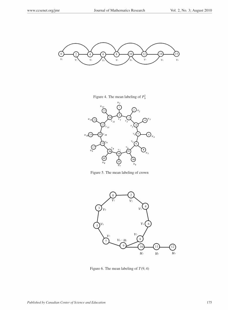
www.ccsenet.org/jmr Journal of Mathematics Research Vol. 2, No. 3; August 2010
0 2 6 8 10 12 14 15
v1 v2 v3 v4 v5 v6 v7 v8 v9
4
Figure 4. The mean labeling of P29
0
2
6
9
17
18
19 20
21
22
23
24
u1
3
2
u3
u4
u5
u6u
7
u8
u9
u10
u11
u12
u1
v1 v
2
v3
v4
v5
v6
v7
v8
v9
v10
v11
v12
16
15
14
13
4
5
7
118
10
Figure 5. The mean labeling of crown
9
8
6
4
20
3
5
7
10 11 12
v1 v2
v3
v4
v5
v6 u1
v7
v8
v9
u2 u3 u4
Figure 6. The mean labeling of T (9, 4)
Published by Canadian Center of Science and Education 175

www.ccsenet.org/jmr Journal of Mathematics Research Vol. 2, No. 3; August 2010
1 4 8 11 14
0 3 5 7 10 13
e1 e2 e3 e4 e5
v1 v2 v3 v4 v6v5
Figure 7. The mean labeling of M(P6)
176 ISSN 1916-9795 E-ISSN 1916-9809

www.ccsenet.org/mas Modern Applied Science Vol. 4, No. 10; October 2010
Published by Canadian Center of Science and Education 65
Odd Graceful Labeling of Some New Graphs
S K Vaidya (corresponding author)
Department of Mathematics, Saurashtra University
Rajkot 360 005, Gujarat, India
E-mail: [email protected]
Lekha Bijukumar
Shanker Sinh Vaghela Bapu Institute of Technology
Gandhinagar Gujarat (INDIA)
E-mail: [email protected]
Abstract
In this work some new odd graceful graphs are investigated. We prove that the graph obtained by joining two copies of even cycle Cn with path Pk and two copies of even cycle Cn sharing a common edge are odd graceful graphs. In addition to this we derive that the splitting graph of K1, n as well as the tensor product of K1,n and P2 admits odd graceful labeling.
Keywords: Odd graceful labeling, Splitting graph, Tensor product
1. Introduction
We begin with simple, finite and undirected graph ( ( ), ( ))G V G E G with p vertices and q edges. For
standard terminology and notations we follow (Harary F., 1972). We will provide brief summary of definitions and other information which serve as prerequisites for the present investigations. Definition 1.1 If the vertices are assigned values subject to certain conditions then it is known as graph labeling. Labeled graphs have many diversified applications in coding theory particularly for missile guidance codes, design of good radar type codes and convolution codes with optimal autocorrelation properties. A systematic study of variety of applications of graph labeling is carried out by (Bloom G.S. and Golomb S.W., 1977). For detailed survey on graph labeling and related results we refer to (Gallian J.A., 2009). Most of the graph labeling schemes found their origin with graceful labeling which was introduced by (Rosa A., 1967) . Definition 1.2 A function f is called graceful labeling of graph G if : {0,1,..., }f V q is injective and the
induced function * : {1, 2,..., }f E q defined as *( ) ( ) ( )f e uv f u f v is bijective. A graph
which admits graceful labeling is called a graceful graph. Many researchers have carried out significant work on graceful labeling. For e.g. In (Golomb S.W.,1972) it has been proved that complete graph Kn is not graceful for 5n . In (Drake A and Redl T.A., 2006) the non graceful Eulerian graphs are enumerated. The famous Ringel-Kotzig graceful tree conjecture and illustrious work in (Kotzig A., 1973) brought a tide of labeling problems having graceful theme. The present work is targeted to discuss one such labeling known as odd graceful labeling which is defined as follows. Definition 1.3 A graph G = (V (G),E(G)) with p vertices and q edges is said to admit odd graceful labeling if
: ( ) {0,1,..., 2 1}f V G q is injective and the induced function * : ( ) {1,3,5,..., 2 1}f E G q
defined as *( ) ( ) ( )f e uv f u f v is bijective. A graph which admits odd graceful labeling is called an
odd graceful graph. (Gnanajothi R.B.,1991) introduced the concept of odd graceful graphs and she has proved many results on this newly defined concept. (Kathiresan K.M.,2008) has discussed odd gracefulness of ladders and graphs obtained from them by subdividing each step exactly once. (Sekar C.,2002) has proved that the splitting graph of path Pn and the splitting graph of even cycle Cn are odd graceful graphs.
Definition 1.4 For a graph G the splitting graph is obtained by adding to each vertex v, a new vertex 'v so that 'v is adjacent to every vertex that is adjacent to v in G.

www.ccsenet.org/mas Modern Applied Science Vol. 4, No. 10; October 2010
ISSN 1913-1844 E-ISSN 1913-1852 66
Definition 1.5 The tensor product of two graphs G1 and G2 denoted by G1(Tp)G2 has vertex set
1 2 1 2( ( ) ) ( ) ( )pV G T G V G V G and the edge set
1 2 1 1 2 2 1 2 1( ( ) ) {( , )( , ) / ( )pE G T G u v u v u u E G and 1 2 2( )}v v E G
Here we prove that the graph obtained by joining two copies of even cycles by path Pk, two copies of even cycles
sharing a common edge, splitting graph of 1,nK are graceful graphs. We also show that tensor product of 1,nK and
P2 admits odd graceful labeling. 2. Main Results Theorem 2.1 The graph obtained by joining two copies of cycle Cn of even order with the path Pk admits odd graceful labeling.
Proof: Let 1 2, ,..., nv v v be the vertices of cycle Cn and 1 2, ,..., ku u u be the vertices of path Pk . Consider
two copies of Cn of even order. Let G be the graph obtained by connecting two copies of Cn with path Pk. Let
1 2, ,..., nv v v , 1 2 [ ( 2)] 1 2 ( 2), ,..., ,n n n k n n kv v v v be the vertices of G and these vertices form a spanning path in
G. In this spanning path the vertex nv is the vertex common to the first copy of Cn and path Pk as well as the vertex
[ ( 2)] 1n kv is the vertex common to the second copy of Cn and path Pk. Define : ( ) {0,1, 2,..., 2 1}f V G q
as follows. For 1 1i n
( ) 1if v i ; i is odd.
(4 2 ) ( 1)n k i ; i is even.
For 3
12
nn i k
( ) 1if v i ; i is even.
(4 2 ) ( 1)n k i ; i is odd
For 3
2 22
nk i n k .
( ) (4 2 ) ( 1)if v n k i ; i is odd
1i ; i is even. In accordance with the above labeling pattern the graph under consideration admits odd graceful labeling. Illustration 2.2 Consider the graph obtained by attaching two copies of C10 by P5. The labeling pattern is as shown in Fig 1. Theorem 2.3 Two copies of even cycle Cn sharing a common edge is an odd graceful graph.
Proof: Let 1 2, ,..., nv v v be the vertices of cycle Cn of even order. Consider two copies of cycle Cn. Let G with
( ) 2 2V G n and ( ) 2 1E G n denotes the graph for two copies of even cycle Cn sharing a common
edge. Without loss of generality let this edge be 2 3
2 2
n ne v v . To define : ( ) {0,1, 2,..., 2 1}f V G q two
cases are to be considered. Case 1: 0(mod 4).n
For 1 1i n
( ) 1if v i ; i is odd.
= 4 ( 1)n i ; i is even.
For 3
22
nn i
( ) 1if v i ; i is even.
= 4 ( 1)n i ; i is odd
For 3 2
2 22
ni n

www.ccsenet.org/mas Modern Applied Science Vol. 4, No. 10; October 2010
Published by Canadian Center of Science and Education 67
( ) 1if v i ; i is even.
= 4 3n i ; i is odd. Case 2: 2(mod 4)n
For 1 i n
( ) 1if v i ; i is odd.
= 4 ( 1)n i ; i is even.
For 3
22
nn i
( ) 1if v i ; i is even.
= 4 ( 1)n i ; i is odd
For 3 2
2 22
ni n
( ) 1if v i ; i is even.
= 4 ( 1)n i ; i is odd.
Above defined labeling pattern exhausts all possibilities and in each case the graph under consideration admits graceful labeling. Illustration 2.4 Consider two copies of cycle C8 sharing a common edge. The labeling pattern is as shown in Fig 2. Theorem 2.5 Splitting graph of a star admits odd graceful labeling.
Proof: Let 1 2, , ,..., nv v v v be the vertices of star 1,nK with v be the apex vertex. Let G be the splitting graph of
1,nK and 'v , 1 2', ',..., 'nv v v be the newly added vertices in 1,nK to form G. Define
: ( ) {0,1, 2,..., 2 1}f V G q by
( ) 0f v
( ) 6 4 3if v n i ; for 1 i n
( ') 2f v
( ') 2 1if v i ; for 1 i n
In view of the above defined labeling pattern G admits odd graceful labeling.
Illustration 2.6 Fig 3 shows the labeling pattern of the splitting graph of 1,4K .
Theorem 2.7 1, 2( )n pK T P is an odd graceful graph.
Proof: Let 1 2 1, ,..., ,n nu u u u be the vertices of star 1,nK , with u1 be the apex vertex. Let v1,v2 be the vertices of
P2. Let G be the graph 1, 2( )n pK T P . We divide the vertex of G into two disjoint sets
1 1{( , ) / 1, 2,..., 1}iT u v i n and 2 2{( , ) / 1, 2,..., 1}iT u v i n .
Define : ( ) {0,1, 2,..., 2 1}f V G q as follows.
1( , ) 2( 1)if u v i ; for 1 1i n
1 2( , ) 1f u v
2( , ) 2( ) 3if u v n i ; for 2 1i n
The above defined function f provides graceful labeling for tensor product of K1,n and path P2. That is,
1, 2( )n pK T P is an odd graceful graph.
Illustration 2.8 In Fig 4 the graph 1,4 2( )pK T P and its odd graceful labeling is shown.
3. Concluding Remarks
Gracefulness and odd gracefulness of a graph are two entirely different concepts. A graph may possess one or both of these or neither. In the present work we investigate four new families of odd graceful graphs. To investigate similar results for other graph families and in the context of different labeling techniques is an open area of research.
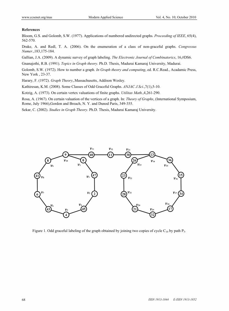
www.ccsenet.org/mas Modern Applied Science Vol. 4, No. 10; October 2010
ISSN 1913-1844 E-ISSN 1913-1852 68
References
Bloom, G.S. and Golomb, S.W. (1977). Applications of numbered undirected graphs. Proceeding of IEEE, 65(4), 562-570.
Drake, A. and Redl, T. A. (2006). On the enumeration of a class of non-graceful graphs. Congressus Numer.,183,175-184.
Gallian, J.A. (2009). A dynamic survey of graph labeling. The Electronic Journal of Combinatorics, 16,#DS6.
Gnanajothi, R.B. (1991). Topics in Graph theory. Ph.D. Thesis, Madurai Kamaraj University, Madurai.
Golomb, S.W. (1972). How to number a graph. In Graph theory and computing, ed. R.C.Read., Acadamic Press, New York , 23-37.
Harary, F. (1972). Graph Theory,.Massachusetts, Addison Wesley.
Kathiresan, K.M. (2008). Some Classes of Odd Graceful Graphs. ANJAC J.Sci.,7(1),5-10.
Kotzig, A. (1973). On certain vertex valuations of finite graphs. Utilitas Math.,4,261-290.
Rosa, A. (1967). On certain valuation of the vertices of a graph. In: Theory of Graphs, (International Symposium, Rome, July 1966),Gordon and Breach, N. Y. and Dunod Paris, 349-355.
Sekar, C. (2002). Studies in Graph Theory. Ph.D. Thesis, Madurai Kamaraj University.
Figure 1. Odd graceful labeling of the graph obtained by joining two copies of cycle C10 by path P5.

www.ccsenet.org/mas Modern Applied Science Vol. 4, No. 10; October 2010
Published by Canadian Center of Science and Education 69
Figure 2. Odd graceful labeling of two copies of cycle C8 sharing a common edge.
Figure 3. Odd graceful labeling of the splitting graph of K1,4.
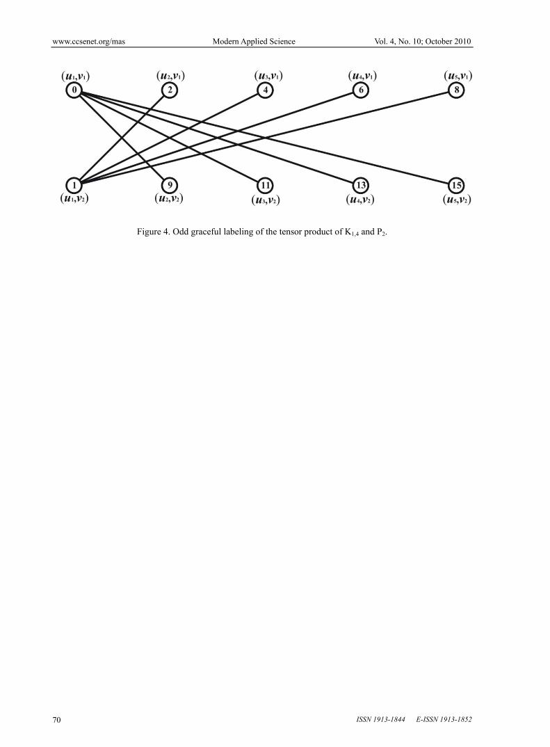
www.ccsenet.org/mas Modern Applied Science Vol. 4, No. 10; October 2010
ISSN 1913-1844 E-ISSN 1913-1852 70
Figure 4. Odd graceful labeling of the tensor product of K1,4 and P2.

Int. J. Open Problems Compt. Math., Vol. 3, No. 5, December 2010ISSN 1998-6262; Copyright c©ICSRS Publication, 2010www.i-csrs.org
New Families of Odd Graceful Graphs
S.K. Vaidya1 and B. Lekha2
1Saurashtra University, Rajkot - 360005, GUJARAT (INDIA)e-mail:[email protected]
2Shanker Sinh Vaghela Bapu Institute of Technology,Gandhinagar, GUJARAT (INDIA)
e-mail:[email protected]
AbstractIn this work some new odd graceful graphs are investigated.
We prove that the graph obtained by fusing all the n verticesof Cn of even order with the apex vertices of n copies of K1,m
admits odd graceful labeling. In addition to this we show thatthe shadow graphs of path Pn and star K1,n are odd gracefulgraphs.
Keywords: Graceful graph,Graceful labeling,Odd graceful graph, Odd grace-ful labeling,Shadow graph.
1 Introduction
We begin with simple,finite,connected and undirected graph G = (V (G), E(G))with p vertices and q edges. For standard terminology and notations we followHarary [4]. We will provide brief summary of definitions and other informationwhich are prerequisites for the present investigations.
Definition 1.1 If the vertices are assigned values subject to certain condi-tions then it is known as graph labeling.
For detailed survey on graph labeling we refer to Gallian [2]
Definition 1.2 A function f is called graceful labeling of graph G if f :V → {0, 1, . . . , q} is injective and the induced function f ∗ : E → {1, 2, . . . , q}defined as f ∗(e = uv) = |f(u)−f(v)| is bijective.A graph which admits gracefullabeling is called a graceful graph.

New Families of Odd Graceful Graphs 167
The study of graceful graphs and graceful labeling methods was introducedby Rosa[6]. While the graceful labeling of graphs was perceived to be primar-ily theoretical subject in the field of graph theory and discrete mathematics.But it is now accepted that gracefully labeled graphs often serve as modelsin a wide range of applications. Such applications including coding theoryand communication net work addressing. The brief survey on applications ofgracefully labeled graphs is reported in Bloom and Golomb [1]. The famousgraceful tree conjecture and many illustrious works brought a tide of labelingscheme having graceful theme. The present work is targeted to discuss onesuch labeling known as odd graceful labeling which is defined as follows.
Definition 1.3 A graph G=(V(G),E(G)) with p vertices and q edges is saidto admit an odd graceful labeling if f : V (G) → {0, 1, 2, . . . , 2q − 1} injectiveand the induced function f* : E(G) → {1, 3, 5, . . . , 2q − 1} defined as f*(e =uv) = |f(u)− f(v)| is bijective. The graph which admits odd graceful labelingis called an odd graceful graph.
The above concept was introduced by Gnanajothi [3] and in the same papershe investigated several results on this newly defined concept.Gracefulness and odd gracefulness are two entirely different concepts. A graphmay posses one or both of these or neither. Kathiresan [5] has discussed oddgracefulness of ladders and the graphs obtained from them by subdividingeach step exactly once. Sekar [7] has proved that the splitting graph of pathPn and the splitting graph of even cycle Cn are odd graceful graphs. In thepresent work we investigate odd graceful labeling for some cycle related andstar related graphs generated by various graph operations.
2 Main Results
Theorem 2.1 The graph obtained by fusing all the n vertices of cycle Cn
of even order with the apex vertices of n copies of K1,m admits odd gracefullabeling.
Proof: Let Cn be a cycle of even order with v1,v2,. . . , vn be its vertices and Gbe the graph obtained by fusing all the n vertices vi of Cn with the apex verticesof star K1,m. Denote the pendant vertices of K1,m by vij where 1 ≤ i ≤ n and1 ≤ j ≤ m. Then G is a graph with |V (G)| = n + nm and |E(G)| = n + nm.To define f : V (G) → {0, 1, 2, . . . , 2q − 1} we consider following two cases.
Case 1: n ≡ 0(mod4) .
For 1 ≤ i ≤ n2

168 S.K. Vaidya et al.
f(vi) = (m + 1)(2n− i) + 1; i is even=(m + 1)(i− 1); i is odd
For n2
+ 1 ≤ i ≤ n
f(vi) = (m + 1)(2n− i) + 1; i is even=(m + 1)(i− 3) + 2(m + 2); i is odd
For 1 ≤ i ≤ n2; 1 ≤ j ≤ m
f(vij)=(m + 1)(2n− i + 1)− 2j + 1 ; if i is odd=(m + 1)(i− 2) + 2j; if i is even
For n2
+ 1 ≤ i ≤ n; 1 ≤ j ≤ m
f(vij)=(m + 1)(2n− i + 1)− 2j + 1 ; if i is odd=(m + 1)(i− 4) + 2(m + j + 2); if i is even
Case 2: n ≡ 2(mod4) .
For 1 ≤ i ≤ n2
+ 1
f(vi) = (m + 1)(2n− i) + 1; i is even=(m + 1)(i− 1); i is odd
For n2
+ 2 ≤ i ≤ n− 1
f(vi) = (m + 1)(2n− i) + 1; i is even=(m + 1)(i− 3) + 2(m + 2); i is odd
f(vn) = (m + 1)(2n− i)− 1
For 1 ≤ i ≤ n2; 1 ≤ j ≤ m
f(vij)=(m + 1)(2n− i + 1)− 2j + 1 ; if i is odd=(m + 1)(i− 2) + 2j; if i is even
For n2
+ 1 ≤ i ≤ n− 1; 1 ≤ j ≤ m
f(vij)=(m + 1)(2n− i + 1)− 2j + 1 ; if i is odd=(m + 1)(i− 2) + 2(j + 1); if i is even
f(vnj)=(m + 1)(n− 2) + 2(j + 1); for 1 ≤ j ≤ m− 1=(m + 1)(n− 2) + 2(2j + 1); forj = m
The above defined function f exhausts all the possibilities and the graph underconsideration is an odd graceful graph.

New Families of Odd Graceful Graphs 169
Illustration 2.2 The following Figure 1 shows the labeling pattern of thegraph obtained by fusing each vertex of C8 with the apex vertices of eightcopies of star K1,3.
Fig 1
Definition 2.3 Shadow graph D2(G) of a connected graph G is obtainedby taking two copies of G say G′ and G′′, join each vertex u′ in G′ to theneighbors of the corresponding vertex u′′ in G′′.
Theorem 2.4 The graph D2(Pn) is an odd graceful graph.
Proof: Let G be D2(Pn) then |V (G)| = 2n and |E(G)| = 4(n − 1) and letv1,v2,. . . , vn be the vertices of first copy of path Pn and v′1,v
′2,. . . , v′n be the
vertices of the second copy of path Pn. Define f : V (G) → {0, 1, 2, . . . , 2q − 1}as follows.
f(vi) = 4(i− 1) ; i is odd=4(2n− i)− 1 ; i is even
f(v′i) = 4(i− 1) + 2 ; i is odd=4(2n− i)− 5 ; i is even
The above defined function f provides graceful labeling for D2(Pn).
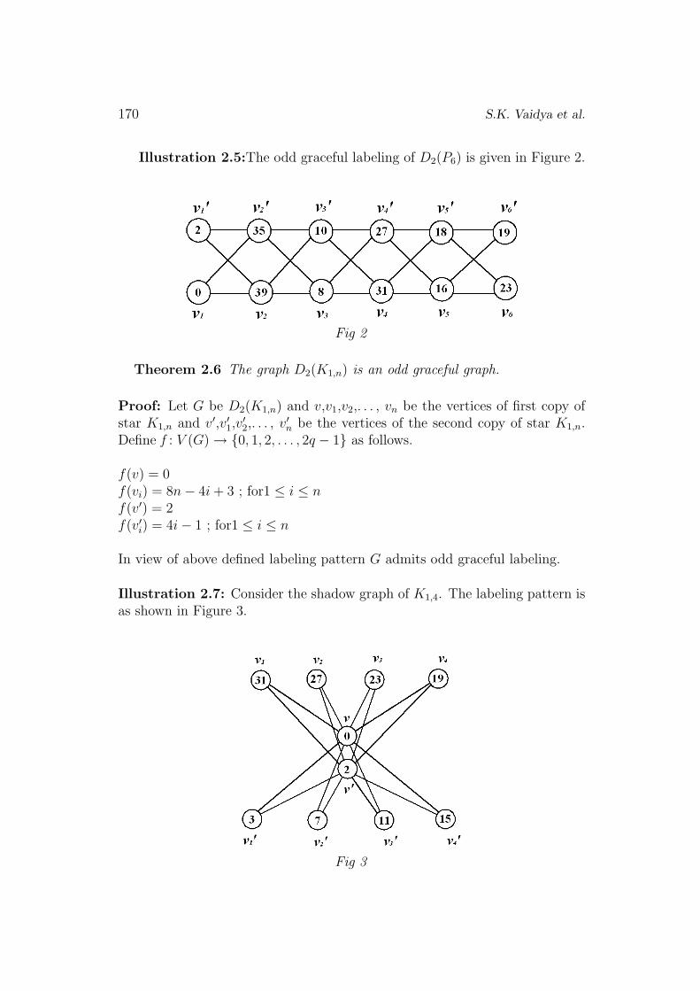
170 S.K. Vaidya et al.
Illustration 2.5:The odd graceful labeling of D2(P6) is given in Figure 2.
Fig 2
Theorem 2.6 The graph D2(K1,n) is an odd graceful graph.
Proof: Let G be D2(K1,n) and v,v1,v2,. . . , vn be the vertices of first copy ofstar K1,n and v′,v′1,v
′2,. . . , v′n be the vertices of the second copy of star K1,n.
Define f : V (G) → {0, 1, 2, . . . , 2q − 1} as follows.
f(v) = 0f(vi) = 8n− 4i + 3 ; for1 ≤ i ≤ nf(v′) = 2f(v′i) = 4i− 1 ; for1 ≤ i ≤ n
In view of above defined labeling pattern G admits odd graceful labeling.
Illustration 2.7: Consider the shadow graph of K1,4. The labeling pattern isas shown in Figure 3.
Fig 3

New Families of Odd Graceful Graphs 171
3 Conclusion
As every graph does not admit odd graceful labeling it is very interesting toinvestigate graphs or graph families which admit odd graceful labeling. In thepresent work we investigate three new families of odd graceful graphs.
4 Open Problems
• Investigate graphs which admit odd graceful labeling.
• Investigate similar results for other graph families and in the context ofvarious graph labeling problems.
• Investigate characterizations for odd gracefulness.
ACKNOWLEDGEMENT: Authors are thankful to anonymous refereesfor their kind comments.
References
[1] G.S.Bloom and S.W.Golomb, Applications of numbered undirectedgraphs, Proceeding of IEEE, 65(4), (1977), pp.562-570.
[2] J. A. Gallian, A dynamic survey of graph labeling, The Electronics Journalof Combinatorics, 17(2010) ]DS6.
[3] R.B. Gnanajothi, Topics in Graph theory, Ph.D Thesis, Madurai KamarajUniversity, Madurai, (1991).
[4] F.Harary, Graph theory, Addison Wesley, Reading, Massachusetts, (1972).
[5] K.M Kathiresan, Some Classes of Odd Graceful Graphs, ANJACJ.Sci.,7(1), (2008), pp.5-10.
[6] A Rosa, On certain valuations of the vertices of a graph, Theory ofgraphs,International Symposium, Rome, July (1966), Gordon and Breach,New York and Dunod Paris, (1967), pp.349-355.
[7] C.Sekar, Studies in Graph Theory, Ph.D. Thesis, Madurai Kamaraj Uni-versity, (2002).

PRAJÑĀ Volume 18, 2010
ISSN 0975 – 2595
Journal of Pure and Applied Sciences
SARDAR PATEL UNIVERSITY VALLABH VIDYANAGAR Gujarat – 388 120, INDIA
www.spuvvn.edu

MEAN LABELING FOR SOME NEW FAMILIES OF GRAPHS
S. K. Vaidya1* and Lekha Bijukumar2
1Saurashtra University, Rajkot-360 005, Gujarat
2Lekha Bijukumar Shanker Sinh Vaghela Bapu Institute of Technology, Gandhinagar, Gujarat
ABSTRACT
Some new families of mean graphs are investigated. We prove that the step ladder graph, total graph of path Pn are mean graphs. In addition to this we derive that two copies of cycle Cn sharing a common edge admits mean labeling. Key words: mean labeling, mean graphs, step ladder graph, total graphs.
INTRODUCTION
We begin with simple, finite, connected and undirected graph G = (V(G),E(G)) with p vertices and q edges. For all other standard terminology and notations we follow Harary [1]. We will provide brief summary of definitions and other information which serve as prerequisites for the present investigations. Definition 1.1 Let Pn be a path on n vertices denoted by (1,1),(1,2),...,(1,n) and with n-1 edges denoted by e1,e2,...,en-1 where ei is the edge joining the vertices (1,i) and (1,i+1). On each edge ei, i = 1, 2, …, n-1 we erect a ladder with n-(i-1) steps including the edge ei. The graph obtained is called a step ladder graph and is denoted by S(Tn), where n denotes the number of vertices in the base. Definition 1.2 The vertices and edges of a graph are called its elements. Two elements of a graph are neighbours if they are either incident or adjacent. The total graph of a graph G is denoted by T(G) is a graph with vertex set and two vertices are adjacent in T(G) when ever they are neighbours in G. Definition 1.3 If the vertices are assigned values subject to certain conditions then it is known as graph labeling. Graph labeling is one of the fascinating areas of graph theory with wide ranging applications. An enormous body of literature has grown around in graph labeling in last five decades. A systematic study of various applications of graph labeling is carried out in Bloom and Golomb [3]. According to Beineke and Hegde [2] graph labeling serves as a frontier between number theory and structure of graphs. For detailed survey on graph labeling we refer to A Dynamic Survey of Graph Labeling by Gallian [4]. Definition 1.4 A function f is called a mean labeling of graph G if
PRAJÑĀ - Journal of Pure and Applied Sciences, Vol. 18: 115 - 116, (2010) ISSN 0975 - 2595
( ) ( )V G E GU
: ( ) {0,1, 2,..., }f V G q→ * : ( ) {1, 2,...,
is injective and the induced function }f E G q→ defined as
( ) ( )*( ) ;2
f u f vf e uv
+= =
if ( ) ( )f u f v+ is even
( ) ( ) 1;2
f u f v+ += if ( ) ( )f u f v+ is odd
is bijective. The graph which admits mean labeling is called a mean graph.
The mean labeling is introduced by Somasundaram and Ponraj [5] and they proved the graphs , , ,n n n m m nP C P P P C× ×
rs in [6] have
1,n
etc. admit mean labeling. The same autho discussed the mean labeling of subdivision of K for 3n ≤
nW does not admit
while in [7]
they proved that the wheel the mean
labeling for . Mean labe t of some graph operations is discussed by Vaidya and Lekha [8]. In the present work three new results corresponding to mean labeling and some new families of mean graphs are investigated. MAIN RESULTS Theorem-2.1: The step ladder graph S(Tn) is a mean graph. Proof: Let Pn be a path on n vertices denoted by (1,1),(1,2),...,(1,n) and with n-1 edges denoted by e1,e2,...,en-1 where ei is the edge joining the vertices (1,i) and (1,i+1). The step ladder graph S(Tn) has vertices denoted by (1,1),(1,2),...,(1,n), (2,1),(2,2),...,(2,n), (3,1),(3,2),...,(3,n-1),...,(n,1),(n,2). In the ordered pair (i,j), i denotes the row (counted from bottom to top) and j denotes the column ( from left to right) in which the vertex occurs. Define
4n ≥ ling in the contex
: ( ( )) {0,1,2,..., }nf V S T q→ as follows. 2( ,1) ( 2) ( 1)f i n n i= + − − − ; 1 i n≤ ≤
12
1 2
(1, ) ( 2) ( ) [( ) ( 1)]j j
k k
f j n n n k n k j−
= =
= + − − − − + − −∑ ∑ ; 2 j n≤ ≤
12
1 2
( , ) ( 2) ( ) [( ) ( 1)] ( 1)j j
k k
f i j n n n k n k j i−
= =
= + − − − − + − − − −∑ ∑ ;
2 , & 2i j n j n i≤ ≤ ≠ + − 2( , 2 ) 2f i n i i+ − = − ; 2 i n≤ ≤
In view of the above defined labeling pattern f is a mean labeling for the step ladder graph S(Tn). That is, S(Tn) is a mean graph. Proof: Let be the vertices of path Pn with n-1
edges denoted b According to the definition of total graph and two vertices are adjacent in T(Pn) if they are neighbours in P . Define
1 2, ,..., nv v v
y 1 2 1, ,..., .ne e e −
n
: ( ( )) {0,1, 2,..., }nf V T P q→ as follows.
1( ) 0f v =
( ) 4( 2) 2;if v i= − + for 2 i n≤ ≤
( ) 4 ;jf e = j for 1 2j n≤ ≤ − *Corresponding author – [email protected]

116 PRAJÑĀ – Journal of Pure and Applied Sciences 18: 115 - 116 December
( ) 4 1;jf e j= − for
Thus f provides a mean labeling for T(Pn). That is, T(Pn) is a mean graph. Illustration 2.2: The Figure 1 shows the labeling pattern for
S(T6).
Fig. 1 Illustration 2.4: The labeling pattern of T(P5) is given in
Figure 2.
Fig. 2 Theorem-2.5: Two copies of cycle Cn sharing a common edge
admit mean labeling. Proof: Let be the vertices of cycle Cn. Consider two copies of cy . Let G be the graph for two copies of cycle sharing a common edge in which is a spanning path. Then
1j n= −
1 2, ,..., nv v vcle Cn.
1 2 2 -2, ,..., nv v v
( ) 2 - 2V G n= and ( ) 2 -1E G n= . To
define : ( ) {0,1,2,..., }f V G q→ the following two cases are to be considered. Case 1: n is odd. Without loss of generality assumes that
1 3 12 2
n ne v v+ −= be the
common edge between two copies of Cn. ; for( ) 2( 1)if v i= − 11
2n
i+
≤ ≤
( ) 2 1if v i= − ; for 32
ni n
+≤ ≤
( ) 2(2 2 ) 4if v n i= − − + ; for 3 312
nn i
−+ ≤ ≤
( ) 2(2 2 ) 3if v n i= − − + ; for 3 1 2 22
ni n
−≤ ≤ −
Case 2: n is even. Without loss of generality assume that
2 32 2
ne v v+= n be the
common edge between two copies of Cn. ; for ( ) 2( 1)if v i= − 21
2n
i+
≤ ≤
( ) 2 1if v i= −
( ) 2(2 2 ) 4if v n i= − − + ; for 3 212
nn i
−+ ≤ ≤
( ) 2(2 2 ) 3if v n i= − − + ; for 3 2 22n
i n≤ ≤ −
Then the above defined function f provides mean labeling for two copies of cycle sharing a common edge. Illustration 2.6: The Figure 3 shows the mean labeling pattern for two copies of C10 sharing an edge.
Fig. 3 CONCLUDING REMARKS AND FURTHER SCOPE
As all graphs are not mean graphs it is very interesting to
investigate graphs which admit mean labeling. Here we contribute three new families of mean graphs. It is possible to investigate similar results for other graph families and in the context of different labeling techniques. ACKNOWLEDGEMENT
Authors are highly thankful to anonymous referee for valuable comments and kind suggestions. REFERENCES [1] Harary, F. (1972) Graph Theory, Addison Wesley,
Reading, Massachusetts. [2] Beineke, L. W. and Hegde, S. M. (2001), Strongly
multiplicative graphs, Discuss. Math. Graph Theory, 21: 63-75.
[3] Bloom, G. S. and Golomb, S. W. (1977) Applications of numbered undirected graphs, Proceedings of IEEE, 65(4): pp. 562-570.
[4] Gallian, J. A. (2009) A dynamic survey of graph labeling, The Electronics Journal of Combinatorics, 16 #DS6.
[5] Somasundaram, S. and Ponraj, R. (2003) Some results on mean graphs, Pure and Applied Mathematical Sciences, 58: 29-35.
[6] Somasundaram, S. and Ponraj, R. (2004) On mean graphs of order < 5, J. Decision and Mathematical Sciences, 9: 47-58.
[7] Somasundaram, S. and Ponraj, R. (2003) Non existence of mean labeling for a wheel, Bulletin of Pure and Applied Sciences, 22E: 103-111.
[8] Vaidya, S. K. and Lekha, B. (2010) Mean labeling in the context of some graph operations, Int. Journal of Algorithms, Comp. and Math. 3(1): 1-8.
; for 42
ni n
+≤ ≤

GUIDELINES FOR CONTRIBUTORS The Editorial Board of ‘PRAJNA’ – Journal of Pure and Applied Sciences invites Original Research Papers in
the fields of Basic and Applied Sciences (Biosciences, Chemistry, Computer Science, Electronics Science, Home Science, Materials Science, Mathematics, Physics and Statistics) for the Next Volume of PRAJNA (December 2011), published by Sardar Patel University, Vallabh Vidyanagar, Gujarat – 388120, INDIA.
The soft copies of regular (full-length) research papers (not exceeding 15 typed pages), prepared as per the file format shown below may be submitted for publication through e-mail to Prof. T. V. Ramana Rao, Managing Editor ([email protected]) OR to a Member of the Editorial Board who represents the author’s broad research area with a cc to the Managing Editor latest by August 31, 2011.
Each manuscript must be accompanied by a statement that it has not been published elsewhere and that it has
not been submitted simultaneously for publication elsewhere. Review process: Submitted papers are peer-reviewed by two to three independent reviewers after approval by the Editorial Board. Authors are encouraged to suggest three names of expert reviewers with their e-mail IDs, but selection remains the prerogative of the Editorial Board. Articles of the following categories are also considered for publication in PRAJNA: Short Communications are limited to a maximum of two figures and one table. They should present a complete study that is more limited in scope than is found in full-length papers. The items of manuscript preparation listed above apply to Short Communications with the following differences: (1) Abstracts are limited to 100 words; (2) instead of a separate Materials and Methods section, experimental procedures may be incorporated into Figure Legends and Table footnotes; (3) Results and Discussion should be combined into a single section.
Review Articles intended to provide concise in-depth reviews of both established and new areas and summarize recent insights in specific research areas within the scope of PRAJNA are solicited by the Editorial Board from leading researchers. The manuscript of this category should be limited to 5,000 words with an abstract of no more than 250 words, a maximum of 5 tables and figures (total), and up to 50 references. Word count includes only the main body of text (i.e., not tables, figures, abstracts or references). Commentaries call attention to papers of particular note and are written at the invitation of the Editorial Board. Perspectives present a viewpoint on an important area of research and are written only at the invitation of the Editorial Board. Perspectives focus on a specific field or subfield within a larger discipline and discuss current advances and future directions. Perspectives are of broad interest for non-specialists and may add personal insight to a field. Letters are brief comments that contribute to the discussion of a research article published in the last issue of PRAJNA. Letters may not include requests to cite the letter writer's work, accusations of misconduct, or personal comments to an author. Letters are limited to 500 words and no more than five references. Letters must be submitted within 3 months of the publication date of the subject article. Also announcement of forthcoming Seminars / Conferences / Symposia / Workshops etc. will be considered for publication in PRAJNA. File format for soft copies: Texts (should be of Times New Roman with 9 point for Abstract and 11 point for other matter) and Tables, if any, must be saved in *.doc (Word) or *.rtf (rich text) format, graphs in Excel and for illustrations (diagrams, maps, drawings, etc.), the TIF format (300 dpi minimal resolution) is the most appropriate (*.TIF or *.JPEG extension). Instructions for preparation of manuscripts: 1. The paper should be written in English and neatly typed with double spacing. 2. The title of the paper and the name(s) of the author(s) be in capital letters. The name of the institution be given in
small letters below the name (s) of the author(s). 3. The ‘Abstract of the paper, in not more than 150 words, should be provided on a separate page along with 4-6
keywords. 4. The sub-titles, e.g. INTRODUCTION, should be written in capital letters.
167

5. Displayed formulae, mathematical equations and expressions should be numbered serially. Table should be with a title in addition to a serial number for it.
6. Photographs / Figures should be original with good contrast so as to be in a form suitable for direct reproduction / scanning.
7. Footnotes are not normally allowed, except to identify the author for correspondence. 8. All figures must be numbered serially as they appear in the text, and their legends / captions should necessarily be
provided. 9. References should be numbered in brackets [ ] in the order of appearance in the text. All the references in the
bibliographic list must correspond to in-text references and vice versa. Abbreviated periodical titles should follow standard subject Abstracts. Names which are not listed by any standard subject indexing organizations should be spelled out in full.
10. All references should be clear and follow the examples below: Periodical articles
[2] Sadqui, M., Fushman, D. and Munoz, V. (2006) Atom – by – atom analysis of global downhill protein folding. Nature, 442: 317 – 321.
Books [16] Stebbins, G. L. (1974) Flowering plants: Evolution above the species level, Arnold Press, London, pp. 1 –
399. Chapters from a book
[19] Schafer, H. and Muyzer, G. (2001) Denaturing gradient gel electrophoresis in marine microbial ecology. In Methods in Microbiology (Ed. Paul, J. H.), Academic Press, London, Vol. 30, pp. 425 – 468.
Thesis or other diplomas [21] Nayaka, S. (2004) The visionary studies on the lichen genus Lecanora sensu lato in India. Ph. D. Thesis,
Dr. R. M. L. Avadh University, Faizabad, India. Conference proceedings
[4] Mohapatra, G. C. (1981) Environment and culture of early man in the valley of rivers Chenab and Ravi, western sub-Himalayas. In Proceedings X Congress of IUPPS, Mexico, pp. 90 – 123.
Online documentation [9] Koning, R. E. (1994). Home Page for Ross Koning. Retrieved 26-6-2009 from Plant Physiology
Information Website: http://plantphys.info/index.html. Note: Manuscripts prepared faithfully in accordance with the instructions will accelerate their processing towards publication; otherwise it would be delayed in view of their expected re-submission.
For and on behalf of Editorial Board, PRAJNA
Prof. T. V. Ramana Rao Managing Editor, PRAJNA
B R Doshi School of Biosciences, Satellite Campus, Vadtal Road,
Sardar Patel University, VALLABH VIDYANAGAR
Gujarat – 388120 Phone: (Lab): 02692-234412 Extn. 111
Mobile: 98254 38147 Fax: 02692-237258 /236475
e-mail: [email protected] Website:www.spuvvn.edu
NOTE: This information may be kindly circulated among your colleagues.
168


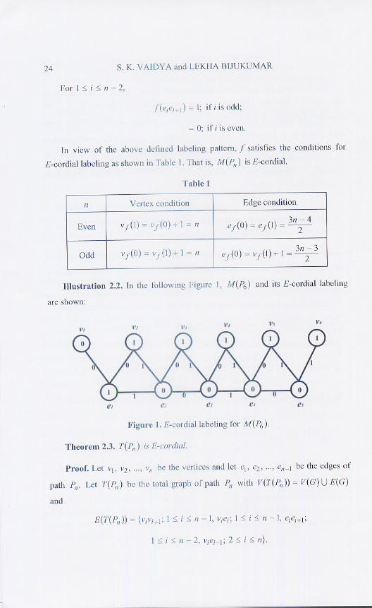

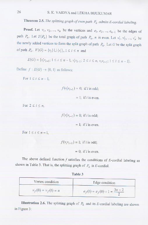
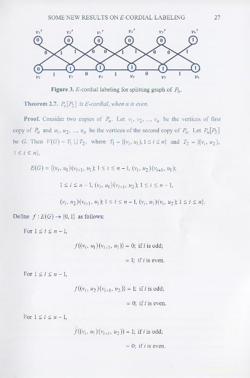


International Journal of Mathematics and Soft ComputingVol.1, No.1 (2011), 37 - 45 ISSN 2249 - 3328
Some new graceful graphs
1 S.K.VaidyaSaurashtra University, Rajkot - 360005,Gujarat, India.
E-mail: [email protected]
Lekha BijukumarShanker Sinh Vaghela Bapu Institute of Technology,
E-mail: [email protected]
Abstract
In this paper we show that the graphs obtained by duplication of an ar-
bitrary vertex in cycleCn as well as duplication of an arbitrary edge in even
cycleCn are graceful graphs. In addition, we derive that the joint sum of two
copies of cycleCn admits graceful labeling.
Keywords: Graceful graphs, Duplication of a vertex, Joint sum.
AMS Subject Classification(2010):05C78.
1 Introduction
We begin with simple, finite, connected and undirected graphG = (V, E) with p
vertices andq edges. For all other standard terminology and notations we follow
Harary[6]. We give a brief summary of definitions and other information which are
useful for the present investigations.
Definition 1.1. If the vertices are assigned values subject to certain conditions thenit is known as graph labeling.
For a dynamic survey on graph labeling we refer to Gallian[4]. A system-
atic study of various applications of graph labeling is carried out in Bloom and
Golomb[2].
Definition 1.2. A function f is called graceful labelingof a graph G if f : V →{0, 1, . . . , q} is injective and the induced function f ∗ : E → {1, . . . , q} defined asf ∗(e = uv) = |f(u)− f(v)| is bijective. A graph which admits graceful labeling iscalled a graceful graph.
1Corresponding author
37
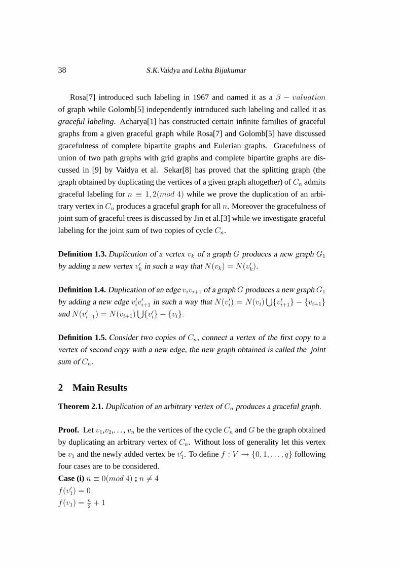
38 S.K.Vaidya and Lekha Bijukumar
Rosa[7] introduced such labeling in 1967 and named it as aβ − valuation
of graph while Golomb[5] independently introduced such labeling and called it as
graceful labeling. Acharya[1] has constructed certain infinite families of graceful
graphs from a given graceful graph while Rosa[7] and Golomb[5] have discussed
gracefulness of complete bipartite graphs and Eulerian graphs. Gracefulness of
union of two path graphs with grid graphs and complete bipartite graphs are dis-
cussed in [9] by Vaidya et al. Sekar[8] has proved that the splitting graph (the
graph obtained by duplicating the vertices of a given graph altogether) ofCn admits
graceful labeling forn ≡ 1, 2(mod 4) while we prove the duplication of an arbi-
trary vertex inCn produces a graceful graph for alln. Moreover the gracefulness of
joint sum of graceful trees is discussed by Jin et al.[3] while we investigate graceful
labeling for the joint sum of two copies of cycleCn.
Definition 1.3.Duplication of a vertex vk of a graph G produces a new graph G1
by adding a new vertex v′k in such a way that N(vk) = N(v′k).
Definition 1.4. Duplication of an edge vivi+1 of a graph G produces a new graph G1
by adding a new edge v′iv′i+1 in such a way that N(v′i) = N(vi)
⋃{v′i+1} − {vi+1}
and N(v′i+1) = N(vi+1)⋃{v′i} − {vi}.
Definition 1.5. Consider two copies of Cn, connect a vertex of the first copy to avertex of second copy with a new edge, the new graph obtained is called the joint
sumof Cn.
2 Main Results
Theorem 2.1.Duplication of an arbitrary vertex of Cn produces a graceful graph.
Proof. Let v1,v2,. . . ,vn be the vertices of the cycleCn andG be the graph obtained
by duplicating an arbitrary vertex ofCn. Without loss of generality let this vertex
bev1 and the newly added vertex bev′1. To definef : V → {0, 1, . . . , q} following
four cases are to be considered.
Case (i)n ≡ 0(mod 4) ; n 6= 4
f(v′1) = 0
f(v1) = n2
+ 1

Some new graceful graphs 39
For2 ≤ i ≤ n2
+ 2
f(vi) = (n + 2)− ( i−22
); wheni is even.
= i−12
; wheni is odd.
For n2
+ 3 ≤ i ≤ n
f(vi) = (n + 2)− ( i−12
); wheni is odd.
= i−22
; wheni is even.
The case whenn = 4 is to be dealt separately and the graph is labeled as shown in
Figure 1.
v1'
v1
v2
v3
v40
6
3
5
4
Figure 1: Duplication of a vertex inC4 and its graceful labeling
Case (ii)n ≡ 1(mod 4)
f(v′1) = 0
f(v1) = n+12
For2 ≤ i ≤ n+12
f(vi) = (n + 2)− ( i−22
); wheni is even.
= i−12
; wheni is odd.
For n+32≤ i ≤ n
f(vi) = i2; wheni is even.
= (n + 2)− ( i−12
); wheni is odd.
Case (iii)n ≡ 2(mod 4) ; n 6= 6
f(v′1)=0
f(v1) = n2+3
For 2≤i≤ n+42
f(vi) = (n + 2)− ( i−22
); wheni is even.
= i−12
; wheni is odd.
f(vi)= i2; for i = n+4
2+ 1
For n+82≤ i ≤ n

40 S.K.Vaidya and Lekha Bijukumar
f(vi) = (n + 2)− ( i−32
); wheni is odd.
= i+22
; wheni is even.
Forn = 6; the corresponding graph and its graceful labeling is shown in Figure 2.
v1
v2
v3
v4
v5
v6
v1'
1
0
8
4
2
3
6
Figure 2: Duplication of a vertex inC6 and its graceful labeling
Case (iv)n ≡ 3(mod 4)
f(v′1)=0
f(v1) = n+12
For 2≤i≤ n+12
f(vi) = (n + 2)− ( i−22
); wheni is even.
= i−12
; wheni is odd.
For n+32≤ i ≤ n
f(vi) = (n + 2)− ( i−12
); wheni is odd.
= i2; wheni is even.
In view of the above defined labeling patternf is a graceful labeling for the graph
obtained by the duplication of an arbitrary vertex in cycleCn.
Illustration 2.2. The graph obtained by duplicating the vertex v1 of cycle C9 isshown in Figure 3.
v1
v1'
v2
v3
v4
v5v6
v7
v8
v9
0
11
5
1
10
23
8
4
7
Figure 3: The graceful labeling of duplication of a vertex inC9

Some new graceful graphs 41
Theorem 2.3.Duplication of an edge in cycles of even order admits graceful label-ing.
Proof. Let v1,v2,. . . , vn be the vertices of the cycleCn wheren is even andG be
the graph obtained by duplicating an arbitrary edge ofCn. Without loss of gener-
ality we may assume thate′ = v′1v′2 be the newly added edge to duplicate the edge
e = v1v2 in Cn. To definef : V → {0, 1, . . . , q} following two cases are to be
considered.
Case (i)n ≡ 0(mod 4); n 6= 4, n 6= 8
f(v′1) = n2
+ 4
f(v′2) = n2
For1 ≤ i ≤ n2
+ 2
f(vi) =(n + 3)− i−12
; wheni is odd.
= i−22
; wheni is even.
f(vi) = i−12
; for i = n2
+ 3
For n2
+ 4 ≤ i ≤ n− 1
f(vi) =(n + 3)− i2; wheni is even.
= i−12
; wheni is odd.
f(vn) =n2
+ 2
The labeling for the graphs corresponding toC4 andC8 are to be dealt separately.
The labeling pattern is provided in Figure 4.
v1 v2
v4 v3
v1' v2'
2 3
0 7
5 1
8 4
0
1
92
3
6 10
11
v1 v2
v3
v4
v5v6
v7
v8
v1' v2'
Figure 4: Graceful labeling of edge duplication inC4 andC8
Case (ii)n ≡ 2(mod 4)
f(v′1) = n2− 1
f(v′2) = n2

42 S.K.Vaidya and Lekha Bijukumar
For1 ≤ i ≤ n2
+ 2
f(vi) =(n + 3)− i−12
; wheni is odd.
= i−22
; wheni is even.
For n2
+ 3 ≤ i ≤ n
f(vi) =(n + 3)− i+22
; wheni is even.
= i−32
; wheni is odd.
The above defined functionf provides graceful labeling for the graph obtained by
the duplication of an edge in cycleCn.
Illustration 2.4. Consider the graph obtained by duplicating an edge v1v2 in C10.The corresponding graceful labeling is shown in Figure 5.
v1 v2
v3
v4
v5
v6v7
v8
v9
v10
v1' v2'
13
12
11
10
4 5
0
1
2
8
3
7
Figure 5: Edge duplication inC10 and its graceful labeling
Theorem 2.5.The joint sum of two copies of cycle Cn admits graceful labeling.
Proof. We denote the vertices of first copy ofCn by v1,v2,....vn and second copy
by vn+1, vn+2,vn+3,....v2n. Join the two copies ofCn with a new edge andG be the
resultant graph. Without loss of generality we assume that the new edge bevnvn+1,
so thatv1,v2,....vn; vn+1,vn+2,....v2n will form a spanning path in G. To definef :V
→ {0, 1, 2, ....q} the following four cases are to be considered.
Case (i)n ≡ 0(mod 4)
For i ≤ n2− 1
f(vi) = n+i+12
; wheni is odd
= 32n− ( i
2− 1); wheni is even
For n2≤i≤ n− 1
f(vi) = 32n− i
2; wheni is even

Some new graceful graphs 43
= n+i+12
; wheni is odd
For i = n; f(vi) = 0
Forn + 1 ≤ i ≤ 32n
f(vi)=(2n + 1)-( i−n−12
); wheni is odd
= i−n2
; wheni is even
For 3n+22
≤ i ≤ 2n
f(vi)=(2n + 1)− ( i−n+12
); wheni is odd
= i−n2
; wheni is even
Case (ii)n ≡ 1(mod 4)
f(v1)=0
For 2≤i≤ n−12
f(vi) = n + ( i+12
); wheni is odd
= (n + 1)− ( i2); wheni is even
For n+12≤ i ≤ n− 1
f(vi) = (n + 1)− ( i+12
); wheni is odd
= n + ( i+22
); wheni is even
Forn ≤ i ≤ 2n
f(vi) = (2n + 1)-( i−n2
) ; wheni is odd
= i+1−n2
; wheni is even
Case (iii)n ≡ 2(mod 4)
For 1≤ i ≤ n− 2
f(vi)= i2; wheni is even
= (2n + 1)− ( i−12
); wheni is odd
f(vn−1) = f(vn−3)− f(vn−2)− 1
f(vn) = 0
Forn + 1 ≤ i ≤ 3n2− 1
f(vi)= i−12
; wheni is odd
= (2n + 1)-( i−42
); wheni is even
f(vi)= i+12
; for i=3n2
For 3n2
+ 1 ≤ i ≤ 3n2
+ 2
f(vi)= i+22
; wheni is even
= (2n + 1)-( i−52
); wheni is odd

44 S.K.Vaidya and Lekha Bijukumar
For 3n2
+ 3 ≤ i ≤ 2n
f(vi)=(2n + 1)-( i−52
) ; wheni is odd
= i+42
; wheni is even
Case (iv)n ≡ 3(mod 4)
1 ≤ i ≤ n−12
f(vi)=3(n+1)
2− ( i+1
2); wheni is odd
= n+i+12
; wheni is even
Forn+12≤ i ≤ n− 2
f(vi)=3(n+1)
2− ( i+2
2); wheni is even
= n+i+22
; wheni is odd
f(vn−1) = 0
Forn ≤ i ≤ 2n
f(vi)=(2n + 1)-( i−n2
) ; wheni is odd
= i+1−n2
; wheni is even
In the above four cases it is possible to assign labels in such a way that it provides
graceful labeling for the joint sum of two copies of cycleCn.
Illustration 2.6. The joint sum of two copies of C13 is as shown in Figure 6.
v1
v2
v3
v4
v5
v6v7
v8
v9
v10
v11
v12v13 v14
v15
v16
v17
v18
v19
v20v21
v22
v23
v24
v25
v26
0
9
8
1
2
3
4
5
6
7
27
13
15
12
16
1110
18
19
20 26
25
24
23
22
21
Figure 6: Graceful labeling of the joint sum of two copies ofC13
AcknowledgementThe authors are thankful to the anonymous referee for valuable comments and sug-
gestions.

Some new graceful graphs 45
References
[1] B. D. Acharya,Construction of certain infinite families of graceful graphs
from a given graceful graph, Def. Sci.J., 32(3)(1982), 231-236.
[2] G. S. Bloom, S. W. Golomb,Applications of numbered undirected graphs,
Proceeding of IEEE,65(4)(1977), 562-570.
[3] D. Jin, S. Liu, S. Lee, H. Liu, X. Lu, D. Zhang,The joint sum of graceful trees,
Computers Math. Applic., 26(10)(1993), 83-87.
[4] J. A. Gallian,A dynamic survey of graph labeling, The Electronics Journal of
Combinatorics, 17(2010)]DS6.
[5] S. W. Golomb,How to number a graph, in Graph theory and Computing,
R.C.Read,ed., Academic Press, New York(1972), 23-37.
[6] F. Harary,Graph theory, Addison Wesley, Reading, Massachusetts, 1972.
[7] A. Rosa, On certain valuations of the vertices of a graph,Theory of
graphs,International Symposium, Rome, July (1966), Gordon and Breach,
New York and Dunod Paris(1967), 349-355.
[8] C.Sekar,Studies in Graph Theory, Ph.D Thesis, Madurai Kamaraj University,
2002.
[9] S. K. Vaidya, V. J. Kaneria, Sweta Srivastav, N. A. Dani,Gracefulness of union
of two path graphs with grid graph and complete bipartite graph,Proceedings
of the Interanational Conference on Emerging Technologies and Applications
in Engineering and Science, 13-14 Jan 2008, Vol. 1, 616-619.

International J.Math. Combin. Vol.3 (2011), 107-113
New Mean Graphs
S.K.Vaidya
(Saurashtra University, Rajkot-360005, Gujarat, India)
Lekha Bijukumar
(Shanker Sinh Vaghela Bapu Institute of Technology, Gandhinagar, Gujarat, India)
E-mail: [email protected], [email protected]
Abstract: A vertex labeling of G is an assignment f : V (G) → {1, 2, 3, . . . , p + q} be an
injection. For a vertex labeling f, the induced Smarandachely edge m-labeling f∗S for an
edge e = uv, an integer m ≥ 2 is defined by f∗S(e) =
⌈
f(u) + f(v)
m
⌉
. Then f is called a
Smarandachely super m-mean labeling if f(V (G))∪{f∗(e) : e ∈ E(G)} = {1, 2, 3, . . . , p+q}.
Particularly, in the case of m = 2, we know that
f∗(e) =
f(u) + f(v)
2if f(u) + f(v) is even;
f(u) + f(v) + 1
2if f(u) + f(v) is odd.
Such a labeling is usually called a mean labeling. A graph that admits a Smarandachely
super mean m-labeling is called a Smarandachely super m-mean graph, particularly, a mean
graph if m = 2. In this paper, some new families of mean graphs are investigated. We
prove that the graph obtained by two new operations called mutual duplication of a pair of
vertices each from each copy of cycle Cn as well as mutual duplication of a pair of edges each
from each copy of cycle Cn admits mean labeling. More over that mean labeling for shadow
graphs of star K1,n and bistar Bn,n are derived.
Key Words: Smarandachely super m-mean labeling, mean labeling, Smarandachely super
m-mean graph, mean graphs; mutual duplication.
AMS(2010): 05C78
§1. Introduction
We begin with simple,finite,connected and undirected graph G = (V (G), E(G)) with p vertices
and q edges. For all other standard terminology and notations we follow Harary [3]. We will
provide brief summary of definitions and other information which serve as prerequisites for the
present investigations.
1Received February 21, 2011. Accepted September 8, 2011.

108 S.K.Vaidya and Lekha Bijukumar
Definition 1.1 Consider two copies of cycle Cn. Then the mutual duplication of a pair of
vertices vk and v′k respectively from each copy of cycle Cn produces a new graph G such that
N(vk) = N(v′k).
Definition 1.2 Consider two copies of cycle Cn and let ek = vkvk+1 be an edge in the first
copy of Cn with ek−1 = vk−1vk and ek+1 = vk+1vk+2 be its incident edges. Similarly let
e′m = umum+1 be an edge in the second copy of Cn with e′m−1 = um−1um and e′m+1 = um+1um+2
be its incident edges. The mutual duplication of a pair of edges ek, e′m respectively from two
copies of cycle Cn produces a new graph G in such a way that N(vk)− vk+1 = N(um)− um+1
={vk−1, um−1} and N(vk+1)− vk = N(um+1)− um ={vk+2, um+2}.
Definition 1.3 The shadow graph D2(G) of a connected graph G is obtained by taking two
copies of G say G′ and G′′. Join each vertex u′ in G′ to the neighbors of the corresponding
vertex u′′ in G′′.
Definition 1.4 Bistar is the graph obtained by joining the apex vertices of two copies of star
K1,n by an edge.
Definition 1.5 If the vertices are assigned values subject to certain conditions then it is known
as graph labeling.
Graph labeling is one of the fascinating areas of research with wide ranging applications.
Enough literature is available in printed and electronic form on different types of graph labeling
and more than 1200 research papers have been published so far in past four decades. Labeled
graph plays vital role to determine optimal circuit layouts for computers and for the repre-
sentation of compressed data structure. For detailed survey on graph labeling we refer to A
Dynamic Survey of Graph Labeling by Gallian [2]. A systematic study on various applications
of graph labeling is carried out in Bloom and Golomb [1].
Definition 1.6 A vertex labeling of G is an assignment f : V (G) → {1, 2, 3, . . . , p + q} be
an injection. For a vertex labeling f, the induced Smarandachely edge m-labeling f∗S for an
edge e = uv, an integer m ≥ 2 is defined by f∗S(e) =
⌈
f(u) + f(v)
m
⌉
. Then f is called a
Smarandachely super m-mean labeling if f(V (G)) ∪ {f∗(e) : e ∈ E(G)} = {1, 2, 3, . . . , p + q}.
Particularly, in the case of m = 2, we know that
f∗(e) =
f(u) + f(v)
2if f(u) + f(v) is even;
f(u) + f(v) + 1
2if f(u) + f(v) is odd.
Such a labeling is usually called a mean labeling. A graph that admits a Smarandachely super
mean m-labeling is called a Smarandachely super m-mean graph, particularly, a mean graph if
m = 2.
The mean labeling was introduced by Somasundaram and Ponraj [4] and they proved the
graphs Pn, Cn, Pn × Pm, Pm × Cn etc. admit mean labeling. The same authors in [5] have
discussed the mean labeling of subdivision of K1,n for n < 4 while in [6] they proved that the
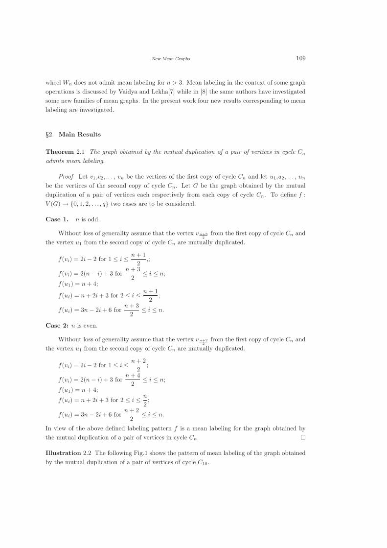
New Mean Graphs 109
wheel Wn does not admit mean labeling for n > 3. Mean labeling in the context of some graph
operations is discussed by Vaidya and Lekha[7] while in [8] the same authors have investigated
some new families of mean graphs. In the present work four new results corresponding to mean
labeling are investigated.
§2. Main Results
Theorem 2.1 The graph obtained by the mutual duplication of a pair of vertices in cycle Cn
admits mean labeling.
Proof Let v1,v2,. . . , vn be the vertices of the first copy of cycle Cn and let u1,u2,. . . , un
be the vertices of the second copy of cycle Cn. Let G be the graph obtained by the mutual
duplication of a pair of vertices each respectively from each copy of cycle Cn. To define f :
V (G) → {0, 1, 2, . . . , q} two cases are to be considered.
Case 1. n is odd.
Without loss of generality assume that the vertex vn+3
2
from the first copy of cycle Cn and
the vertex u1 from the second copy of cycle Cn are mutually duplicated.
f(vi) = 2i− 2 for 1 ≤ i ≤n + 1
2,;
f(vi) = 2(n− i) + 3 forn + 3
2≤ i ≤ n;
f(u1) = n + 4;
f(ui) = n + 2i + 3 for 2 ≤ i ≤n + 1
2;
f(ui) = 3n− 2i + 6 forn + 3
2≤ i ≤ n.
Case 2: n is even.
Without loss of generality assume that the vertex vn+2
2
from the first copy of cycle Cn and
the vertex u1 from the second copy of cycle Cn are mutually duplicated.
f(vi) = 2i− 2 for 1 ≤ i ≤n + 2
2;
f(vi) = 2(n− i) + 3 forn + 4
2≤ i ≤ n;
f(u1) = n + 4;
f(ui) = n + 2i + 3 for 2 ≤ i ≤n
2;
f(ui) = 3n− 2i + 6 forn + 2
2≤ i ≤ n.
In view of the above defined labeling pattern f is a mean labeling for the graph obtained by
the mutual duplication of a pair of vertices in cycle Cn. �
Illustration 2.2 The following Fig.1 shows the pattern of mean labeling of the graph obtained
by the mutual duplication of a pair of vertices of cycle C10.

110 S.K.Vaidya and Lekha Bijukumar
100 14 24
4 6
2 8
5 7
3 9
19 21
17 23
18 20
16 22
v1
v2
v3 v4
v5
v6
v7
v8v9
v10
u1
u2
u3 u4
u5
u6
u7
u8u9
u10
Fig.1
Theorem 2.3 The graph obtained by the mutual duplication of a pair of edges in cycle Cn
admits mean labeling.
Proof Let v1,v2,. . . , vn be the vertices of the first copy of cycle Cn and let u1,u2,. . . , un
be the vertices of the second copy of cycle Cn. Let G be the graph obtained by the mutual
duplication of a pair of edges each respectively from each copy of cycle Cn. To define f : V (G) →
{0, 1, 2, . . . , q} two cases are to be considered.
Case 1. n is odd.
Without loss of generality assume that the edge e= vn+1
2
vn+3
2
from the first copy of cycle
Cn and the edge e′= u1u2 from the second copy of cycle Cn are mutually duplicated.
f(v1) = 0;
f(vi) = 2i− 1 for 2 ≤ i ≤n + 1
2;
f(vi) = 2(n− i) + 2 forn + 3
2≤ i ≤ n;
f(ui) = n + 2i + 2 for 1 ≤ i ≤n + 1
2;
f(ui) = 3n− 2i + 7 forn + 3
2≤ i ≤ n.

New Mean Graphs 111
0
3
5 7
9
8
64
2 v6
v7v8
v9
15
17 19
21
22
20
1816
13
v1
v2
v3 v4
v5 u2
u3 u4
u5
u6
u7
u8u9
u1
Fig.2
Case 2. n is even, n 6= 4.
Without loss of generality assume that the edge e= vn
2+1vn
2+2 from the first copy of cycle
Cn and the edge e′= u1u2 from the second copy of cycle Cn are mutually duplicated.
f(vi) = 2i− 2 for 1 ≤ i ≤n
2+ 1;
f(vi) = 2(n− i) + 3 forn
2+ 2 ≤ i ≤ n;
f(ui) = n + 2i + 2 for 1 ≤ i ≤n
2+ 1;
f(ui) = 3n− 2i + 7 forn
2+ 2 ≤ i ≤ n.
Then above defined function f provides mean labeling for the graph obtained by the mutual
duplication of a pair of edges in Cn. �
Illustration 2.4 The following Fig.2 shows mean labeling for the graph obtained by the mutual
duplication of a pair of edges in cycle C9.
Theorem 2.5 D2(K1,n) is a mean graph.
Proof Consider two copies of K1,n. Let v,v1,v2,. . . , vn be the vertices of the first copy
of K1,n and v′,v′1,v′
2,. . . , v′n be the vertices of the second copy of K1,n where v and v′ are the
respective apex vertices. Let G be D2(K1,n). Define f : V (G) → {0, 1, 2, . . . , q} as follows.
f(v) = 0;
f(vi) = 2i for 1 ≤ i ≤ n;
f(v′) = 4n;
f(v′1) = 4n− 1;
f(v′i) = 4n− 2i + 2 for 2 ≤ i ≤ n.
The above defined function provides the mean labeling of the graph D2(K1,n). �

112 S.K.Vaidya and Lekha Bijukumar
Illustration 2.6 The labeling pattern for D2(K1,4) is given in Fig.3.
2 4 6 8
9
16
15 14 12 10
v
v1 v2 v3 v4
v′
v′
1 v′
2 v′
3 v′
4
Fig.3
Theorem 2.7 D2(Bn,n) is a mean graph.
Proof Consider two copies of Bn,n. Let {u, v, ui, vi, 1 ≤ i ≤ n} and {u′, v′, u′i, v′
i, 1 ≤
i ≤ n} be the corresponding vertex sets of each copy of Bn,n. Let G be D2(Bn,n). Define
f : V (G)→ {0, 1, 2, . . . , q} as follows.
f(u) = 0;
f(ui) = 2i for 1 ≤ i ≤ n;
f(v) = 8n + 1;
f(vi) = 4i + 1 for 1 ≤ i ≤ n− 1;
f(vn) = 4n + 5;
f(u′) = 4n;
f(u′i) = 2(n + i) for 1 ≤ i ≤ n− 1;
f(u′n) = 4n− 1;
f(v′) = 8n + 3;
f(v′i) = 8(n + 1)− 4i for 1 ≤ i ≤ n.
In view of the above defined labeling pattern G admits mean labeling. �
Illustration 2.8 The labeling pattern for D2(B3,3) is given in Fig.4.

New Mean Graphs 113
2 4 6
0
12
8 10 11
u1 u2 u3
u
u′
u′
1 u′
2 u′
3
5 9 17
28 24 20
25
27
v
v1 v2 v3
v′
1 v′
2 v′
3
v′
Fig.4
§3. Concluding Remarks
As all the graphs are not mean graphs it is very interesting to investigate graphs or graph
families which admit mean labeling. Here we contribute two new graph operations and four
new families of mean graphs. Somasundaram and Ponraj have proved that star K1,n is mean
graph for n ≤ 2 and bistar Bm,n (m > n) is mean graph if and only if m < n + 2 while in
this paper we have investigated that the shadow graphs of star K1,n and bistar Bn,n also admit
mean labeling.
To investigate similar results for other graph families and in the context of different labeling
techniques is an open area of research.
References
[1] G.S.Bloom and S.W.Golomb, Applications of numbered undirected graphs, Proceedings of
IEEE, 65(4) (1977), 562-570.
[2] J. A. Gallian, A dynamic survey of graph labeling, The Electronics Journal of Combina-
torics, 17 (2010) ]DS6.
[3] F. Harary, Graph Theory, Addison Wesley, Reading, Massachusetts, 1972.
[4] S. Somasundaram and R. Ponraj, Some results on mean graphs, Pure and Applied Mathe-
matical Sciences, 58 (2003),29-35.
[5] S. Somasundaram and R. Ponraj, On mean graphs of order < 5, J.Decision and Mathe-
matical Sciences, 9 (2004),47-58.
[6] S. Somasundaram and R. Ponraj, Non-existance of mean labeling for a wheel, Bulletin of
Pure and Applied Sciences, 22E (2003),103-111.
[7] S. K.Vaidya and Lekha Bijukumar, Mean labeling in the context of some graph operations,
Int. J of Algorithms, Comp. and Math.,3(1) (2010), 1-8.
[8] S. K.Vaidya and Lekha Bijukumar, Some new families of mean graphs, J. Math. Res., 2(1)
(2010), 169-176.

www.ccsenet.org/jmr Journal of Mathematics Research Vol. 3, No. 4; November 2011
Some New Families of E-Cordial Graphs
S K Vaidya (Corresponding author)
Saurashtra University
Rajkot 360005, GUJARAT, India
E-mail: [email protected]
Lekha Bijukumar
Shanker Sinh Vaghela Bapu Institute of Technology
Gandhinagar, GUJARAT, India
E-mail: [email protected]
Received: May 23, 2011 Accepted: June 27, 2011 Published: November 1, 2011
doi:10.5539/jmr.v3n4p105 URL: http://dx.doi.org/10.5539/jmr.v3n4p105
Abstract
In this paper some new families E-cordial graphs are investigated. We prove that the graphs obtained by duplication of
an arbitrary vertex as well as an arbitrary edge in cycle Cn admit E-cordial labeling. In addition to this we derive that the
joint sum of two copies of cycle Cn, the split graph of cycle Cn of even order and the shadow graph of path Pn for even nare E-cordial graphs.
Keywords: E-cordial labeling, Joint sum, Shadow graphs
AMS Subject classification number(2010): 05C78.
1. Introduction
We begin with simple,finite,connected and undirected graph G = (V(G), E(G)) with p vertices and q edges. For all other
standard terminology and notations we follow (Harary,F.,1972). We will provide brief summary of definitions and other
information which serve as prerequisites for the present investigations.
1.1 Definition: Duplication of a vertex vk of a graph G produces a new graph G1 by adding a new vertex v′k in such a way
that N(vk)=N(v′k).
1.2 Definition: For a graph G the split graph is obtained by duplicating its vertices altogether.
1.3 Definition: Consider a cycle Cn and let ek = vkvk+1 be an edge in it with ek−1 = vk−1vk and ek+1 = vk+1vk+2 be its
incident edges and e′k = v′kv′k+1be a new edge. The duplication of an edge ek by an edge e′k produces a new graph G in
such a way that N(vk)⋂
N(v′k) ={vk−1} and N(vk+1)⋂
N(v′k+1) ={vk+2}.
1.4 Definition: Consider two copies of Cn, connect a vertex of the first copy to a vertex of second copy with a new edge,
the new graph obtained is called the joint sum of Cn.
1.5 Definition: The shadow graph D2(G) of a connected graph G is obtained by taking two copies of G say G′ and G′′.Join each vertex u′ in G′ to the neighbors of the corresponding vertex u′′ in G′′.
1.6 Definition: If the vertices are assigned values subject to certain conditions then it is known as graph labeling.
Graph labeling have often been motivated by practical problems is one of the fascinating areas of research. A systematic
study of various applications of graph labeling is carried out in (Bloom,G.S., and Golomb,S.W.,1977,p.562-570). Labeled
graph plays vital role to determine optimal circuit layouts for computers and for the representation of compressed data
structure. For detailed survey on graph labeling we refer to A Dynamic Survey of Graph Labeling by (Gallian,J.,2010).
1.7 Definition: A function f is called graceful labeling of graph G if f : V → {0, 1, . . . , q} is injective and the induced
function f ∗ : E → {1, . . . , q} defined as f ∗(e = uv) = | f (u) − f (v)| is bijective. A graph which admits graceful labeling is
called a graceful graph.
Graceful labeling was introduced by (Rosa, A., 1967, p.349-355). Many illustrious works on graceful graphs provided the
reason for different ways of labeling of graphs. Some variations of graceful labeling are also introduced. Some of them
are edge graceful labeling, harmonious labeling, fibonacci graceful labeling, odd graceful labeling etc.
Published by Canadian Center of Science and Education 105

www.ccsenet.org/jmr Journal of Mathematics Research Vol. 3, No. 4; November 2011
(Cahit, I., 1987, p.201-207) introduced cordial labeling as a weaker version of graceful labeling and harmonious labeling
which is defined as follows.
1.8 Definition: Let G be a graph. A mapping f : V(G) → {0, 1} is called a binary vertex labeling of G and f (v) is called
the label of the vertex v of G under f .
For an edge e = uv, the induced edge labeling f ∗ : E(G) → {0, 1} is given by f ∗(e = uv) = | f (u) − f (v)|. Let v f (0), v f (1)
be the number of vertices of G having labels 0 and 1 respectively under f and let e f (0), e f (1) be the number of edges of
G having labels 0 and 1 respectively under f ∗.
1.9 Definition: A binary vertex labeling of a graph G is cordial labeling if |v f (0) − v f (1)| ≤ 1 and |e f (0) − e f (1)| ≤ 1. A
graph is cordial if it admits cordial labeling.
1.10 Definition: A graph G = (V(G), E(G)) with p vertices and q edges is said to be edge graceful if there exists a
bijection f : E(G) −→ {1, 2, . . . , q} such that the induced mapping f +: V(G) −→ {0, 1, 2, . . . , p − 1} given by f +(x) =
(∑
f (xy))(mod p) taken over all edges xy is a bijection.
1.11 Definition: Let G = (V(G), E(G)) with p vertices and q edges and f : E(G) → {0, 1}. Define f ∗ on V(G) by
f (v) =∑{ f (uv)/uv ∈ E(G)}(mod 2). The function f is called an E-cordial labeling of G if the number of vertices labeled
0 and the number of vertices labeled 1 differ by at most 1 and the number of edges labeled 0 and the number of edges
labeled 1 differ by at most 1. A graph that admits E-cordial labeling is called E-cordial.
(Yilmaz, R., and Cahit, I., 1997, p.251-266) introduced E-cordial labeling which is a weaker version of edge graceful
labeling having blend of cordial labeling. They proved that the trees with n vertices, Kn, Cn are E-cordial if and only if
n � 2(mod 4) while Km,n admits E-cordial labeling if and only if m + n � 2(mod 4). They observed that the graphs with
p ≡ 2(mod 4) can not be E-cordial. (Devaraj, J., 2004, p.14-18) has shown that Mm,n which is the the mirror graph of Km,n
is E-cordial when m + n is even and the generalized Petersen graph Pn,k is E-cordial when n is even.
2. Main Results
2.1 Theorem: The graph obtained by duplication of an arbitrary vertex of Cn admits E-cordial labeling.
Proof: Let v1, v2, . . . , vn be the vertices of the cycle Cn. Let G be the graph obtained by duplicating an arbitrary vertex of
Cn. Without loss of generality let this vertex be v1 and the newly added vertex be v′1. E(G)={E(Cn), e′, e′′} where e′ = v′1v2
and e′′ = vnv′1.To define f : E(G) → {0, 1} two cases are to be considered.
Case 1: n ≡ 0, 2 (mod 4)
f (e′) = 0
f (e′′) = 1 ;
f (ei) = 0; for i ≡ 1, 0 (mod 4)
=1; for i ≡ 2, 3 (mod 4) and 1 ≤ i ≤ n
Case 2: n ≡ 3 (mod 4)
f (e′) = 0 ;
f (e′′) = 1 ;
f (ei) = 1; for i ≡ 1, 2 (mod 4),
=0; for i ≡ 0, 3 (mod 4) and 1 ≤ i ≤ n
In view of the above defined labeling pattern f satisfies the conditions for E-cordial labeling as shown in Table 1. That is,
the graph obtained by the duplication of an arbitrary vertex in cycle Cn admits E-cordial labeling.
2.2 Illustration: Figure 1 shows the E-cordial labeling of the graph obtained by the duplication of an arbitrary vertex in
cycle C12.
2.3 Theorem: The graph obtained by duplication of an arbitrary edge in Cn admits E-cordial labeling.
Proof: Let v1, v2, . . . , vn be the vertices of the cycle Cn. Let G be the graph obtained by duplicating an arbitrary edge of
Cn. Without loss of generality let this edge be e1 = v1v2 and the newly added edge be e′1 = v′1v′2. E(G)={E(Cn), e′1, e′, e′′}
where e′ = v′2v3 and e′′ = vnv′1. Define f : E(G) → {0, 1} as follows.
Case 1: n ≡ 1, 2 (mod 4)
f (e′1) = 1 ;
106 ISSN 1916-9795 E-ISSN 1916-9809

www.ccsenet.org/jmr Journal of Mathematics Research Vol. 3, No. 4; November 2011
f (e′) = 0 ;
f (e′′) = 1 ;
For 1 ≤ i ≤ n
f (ei) = 0; for i ≡ 0, 1 (mod 4),
=1; for i ≡ 2, 3 (mod 4)
Case 2: n ≡ 3 (mod 4)
f (e′1) = 1 ;
f (e′) = 0 ;
f (e′′) = 1 ;
For 1 ≤ i ≤ n − 1
f (ei) = 0; for i ≡ 0, 1 (mod 4),
=1; for i ≡ 2, 3 (mod 4)
f (en) = 0;
In view of the above defined labeling pattern f satisfies the conditions for E-cordial labeling as shown in Table 2. That is,
the graph obtained by the duplication of an arbitrary edge in cycle Cn is E-cordial.
2.4 Illustration: The E-cordial labeling of the graph obtained by the duplication of an arbitrary edge in cycle C11 is as
shown in Figure 2.
2.5 Theorem: Joint sum of two copies of Cn of even order produces an E-cordial graph.
Proof: We denote the vertices of first copy of Cn by v1,v2,....vn and second copy by v′1, v′2,v′3,....v′n, ei and e′i where 1 ≤ i ≤ nbe the corresponding edges. Join the two copies of Cn with a new edge and let G be the resultant graph. Without loss of
generality we assume that the new edge be e=v1v′1. To define f : E(G) → {0, 1} two cases are to be considered.
Case 1: n ≡ 0 (mod 4)
f (e) = 0 ;
f (ei) = 0; for i ≡ 0, 1 (mod 4),
=1; for i ≡ 2, 3 (mod 4) and 1 ≤ i ≤ n
f (e′i) = 0; for i ≡ 0, 1 (mod 4),
=1; for i ≡ 2, 3 (mod 4) and 1 ≤ i ≤ n
Case 2: n ≡ 2 (mod 4)
f (e) = 1 ;
f (ei) = 0; for i ≡ 0, 1 (mod 4),
=1; for i ≡ 2, 3 (mod 4) and 1 ≤ i ≤ n
f (e′i) = 0; for i ≡ 0, 1 (mod 4),
=1; for i ≡ 2, 3 (mod 4) and 1 ≤ i ≤ n
In view of the above defined labeling pattern f satisfies the conditions for E-cordial labeling as shown in Table 3. That is,
the joint sum of two copies of even cycle Cn is E-cordial.
2.6 Illustration: E-cordial labeling of joint sum of two copies of cycle C10 is shown in Figure 3.
2.7 Theorem: The split graph of Cn of even order is E-cordial.
Proof: Let v1, v2, .... vn be the vertices of cycle Cn and v′1, v′2, .... v′n be the newly added vertices where n is even. Let
G be the split graph of cycle Cn with V(G) = {vi, v′i ; 1 ≤ i ≤ n} and E(G) = {vivi+1; 1 ≤ i ≤ n − 1, vnv1, v′i vi+1; 1 ≤ i ≤n − 1, v′nv1, viv′i+1; 1 ≤ i ≤ n − 1, vnv′1}. To define f : E(G) → {0, 1} two cases are to be considered.
Case 1: n ≡ 0 (mod 4)
For 1 ≤ i ≤ n − 1
Published by Canadian Center of Science and Education 107

www.ccsenet.org/jmr Journal of Mathematics Research Vol. 3, No. 4; November 2011
f (vivi+1) = 0; if i is odd
=1; if i is even.
f (vnv1) = 1
For 1 ≤ i ≤ n − 1
f (viv′i+1) = 0; if i ≡ 1, 2 (mod 4)
=1; if i ≡ 0, 3 (mod 4)
f (vnv′1) = 1
For 1 ≤ i ≤ n − 1
f (v′i vi+1) = 1; if i ≡ 1, 2 (mod 4)
=0; if i ≡ 0, 3 (mod 4)
f (v′nv1) = 0
Case 2: n ≡ 2 (mod 4)
For 1 ≤ i ≤ n − 1
f (vivi+1) = 0; if i is odd
=1; if i is even.
f (vnv1) = 0
For 1 ≤ i ≤ n − 1
f (viv′i+1) = 0; if i ≡ 1, 2 (mod 4)
=1; if i ≡ 0, 3 (mod 4)
f (vnv′1) = 1
For 1 ≤ i ≤ n − 1
f (v′i vi+1) = 1; if i ≡ 1, 2 (mod 4)
=0; if i ≡ 0, 3 (mod 4)
f (v′nv1) = 1
In view of the above defined labeling pattern f satisfies the conditions for E-cordial labeling as shown in Table 5. That is,
the split graph of even cycle Cn is E-cordial.
Illustration 2.8: Figure 4 shows the E-cordial labeling of split graph of cycle C8.
2.9 Theorem: D2(Pn) is E-cordial for even n.
Proof:Let P′n P′′
n be two copies of path Pn. We denote the vertices of first copy of Pn by v′1, v′2, .... v′n and second copy by
v′′1 , v′′2 , .... v′′n . Let G be D2(Pn) with |v(G)| = 2n and |E(G)| = 4n − 4. To define f : E(G) → {0, 1} two cases are to be
considered.
Case 1: n ≡ 0 (mod 4)
For 1 ≤ i ≤ n − 1
f (v′i v′i+1) = 1 ; if i � 3 j
=0; if i = 3 j, j = 1, 2, . . .⌊
n3
⌋For 1 ≤ i ≤ n − 1
f (v′′i v′′i+1) = 0 ; if i � 3 j
=1; if i = 3 j, j = 1, 2, . . .⌊
n3
⌋For 1 ≤ i ≤ n − 2
f (v′′i v′i+1) = 1 ; if i is odd
=0; if i is even
108 ISSN 1916-9795 E-ISSN 1916-9809

www.ccsenet.org/jmr Journal of Mathematics Research Vol. 3, No. 4; November 2011
f (v′′n−1v′n) = 0
For 1 ≤ i ≤ n − 1
f (v′i v′′i+1) = 1 ; if i is odd
=0; if i is even
Case 2: n ≡ 2 (mod 4)
For 1 ≤ i ≤ n − 1
f (v′i v′i+1) = 1 ; if i ≡ 1, 2 (mod 4)
=0; if i ≡ 0, 3 (mod 4)
For 1 ≤ i ≤ n − 1
f (v′′i v′′i+1) = 0 ; if i ≡ 1, 2 (mod 4)
=1; if i ≡ 0, 3 (mod 4)
For 1 ≤ i ≤ n − 2
f (v′i v′′i+1) = 1 ; if i is odd
=0; if i is even
f (v′n−1v′′n ) = 0
For 1 ≤ i ≤ n − 1
f (v′′i v′i+1) = 1 ; if i is odd
=0; if i is even
In view of the above defined labeling pattern f satisfies the conditions for E-cordial labeling as shown in Table 5. That is,
D2(Pn) is E-cordial for even n.
Illustration 2.10: Figure 5 shows the E-cordial labeling of D2(P6).
3. Concluding Remarks
Here we contribute five new families of E-cordial graphs generated by different graph operations. To investigate similar
results for other graph families and in the context of different graph labeling techniques is an open area of research.
Acknowledgment
The authors are highly thankful to the anonymous referees for constructive suggestions and comments.
References
Bloom, G. S. and Golomb, S. W. (1977). Applications of numbered undirected graphs. Proceedings of IEEE, 65(4),
562-570. http://dx.doi.org/10.1109/PROC.1977.10517
Cahit, I. (1987). Cordial Graphs: A weaker version of graceful and harmonious graphs. Ars Combinatoria, 23, 201-207.
Devraj, J. (2004). On edge-cordial graphs.Graph Theory Notes of New York, XLVII, 14-18.
Gallian, J. A. (2010). A dynamic survey of graph labeling. The Electronics Journal of Combinatorics, 17, �DS 6.
Harary, F. (1972). Graph Theory. Addison Wesley, Reading, Massachusetts.
Rosa, A. (1966, 1967). On certain valuation of the vertices of a graph. Theory of graphs, International Symposium, Rome,
New York and Dunod Paris ,349-355.
Yilmaz, R. and Cahit, I. (1997). E-cordial graphs. Ars Combin, 46, 251-266.
Table 1.
n vertex condition edge condition
n � 0(mod 4) v f (0) = v f (1) + 1 = n+22
e f (0) = e f (1) = n+22
n � 2(mod 4) v f (1) = v f (0) + 1 = n+22
e f (0) = e f (1) = n+22
n � 3(mod 4) v f (1) = v f (0) = n+12
e f (1) = e f (0) + 1 = n+32
Published by Canadian Center of Science and Education 109

www.ccsenet.org/jmr Journal of Mathematics Research Vol. 3, No. 4; November 2011
Table 2.
n vertex condition edge condition
n � 1(mod 4) v f (1) = v f (0) + 1 = n+32
e f (0) = e f (1) = n+32
n � 2(mod 4) v f (1) = v f (0) = n+22
e f (1) = e f (0) + 1 = n+42
n � 3(mod 4) v f (0) = v f (1) + 1 = n+32
e f (0) = e f (1) = n+32
Table 3.
n Vertex Condition Edge Condition
n � 0(mod 4) v f (0) = v f (1) = n e f (0) = e f (1) + 1 = n + 1
n � 2(mod 4) v f (0) = v f (1) = n e f (1) = e f (0) + 1 = n + 1
Table 4.
n Vertex Condition Edge Condition
n � 0, 2(mod 4) v f (0) = v f (1) = n e f (0) = e f (1) = 3n2
Table 5.
n Vertex Condition Edge Condition
n � 0, 2(mod 4) v f (0) = v f (1) = n e f (0) = e f (1) = 2n − 2
Figure 1. E-cordial labeling of the graph obtained by duplication of vertex v1 in C12
Figure 2. E-cordial labeling of the graph obtained by duplication of the edge v1v2 in C11
110 ISSN 1916-9795 E-ISSN 1916-9809

www.ccsenet.org/jmr Journal of Mathematics Research Vol. 3, No. 4; November 2011
Figure 3. E-cordial labeling of Joint sum of two copies of C10
Figure 4. E-cordial labeling of split graph of cycle C8
Figure 5. E-cordial labeling of D2(P6)
Published by Canadian Center of Science and Education 111